Table of Contents for
Applied Text Analysis with Python
 Applied Text Analysis with Python
Published by
O'Reilly Media, Inc., 2018
Applied Text Analysis with Python
Published by
O'Reilly Media, Inc., 2018
- Cover
- nav
- Applied Text Analysis with Python
- Applied Text Analysis with Python
- Preface
- 1. Language and Computation
- 2. Building a Custom Corpus
- 3. Corpus Preprocessing and Wrangling
- 4. Text Vectorization and Transformation Pipelines
- 5. Classification for Text Analysis
- 6. Clustering for Text Similarity
- 7. Context-Aware Text Analysis
- 8. Text Visualization
- 9. Graph Analysis of Text
- 10. Chatbots
- 11. Scaling Text Analytics with Multiprocessing and Spark
- 12. Deep Learning and Beyond
- Glossary
- Index
- About the Authors
- Colophon
Chapter 11. Scaling Text Analytics with Multiprocessing and Spark
In the context of language-aware data products, text corpora are not static fixtures, but instead living datasets that constantly grow and change. Take, for instance, a question-and-answer system; in our view this is not only an application that provides answers, but one that collects questions. This means even a relatively modest corpus of questions could quickly grow into a deep asset, capable of training the application to learn better responses in the future.
Unfortunately, text processing techniques are expensive both in terms of space (memory and disk) and time (computational benchmarks). Therefore, as corpora grow, text analysis requires increasingly more computational resources. Perhaps you’ve even experienced how long processing takes on the corpora you’re experimenting on while working through this book! The primary solution to deal with the challenges of large and growing datasets is to employ multiple computational resources (processors, disks, memory) to distribute the workload. When many resources work on different parts of computation simultaneously we say that they are operating in parallel.
Parallelism (parallel or distributed computation) has two primary forms. Task parallelism means that different, independent operations run simultaneously on the same data. Data parallelism implies that the same operation is being applied to many different inputs simultaneously. Both task and data parallelism are often used to accelerate computation from its sequential form (one operation at a time, one after the other) with the intent that the computation becomes faster.
It is important to remember that speed is the name of the game, and that trade-offs exist in a parallel environment. More smaller disks rather than fewer large disks means that data can be read faster off the disk, but each disk can store less and must be read separately. Computations in parallel means that the job gets done more quickly, so long as computations aren’t waiting for others to complete. It takes time and effort to set up resources to perform parallel computation, and if that effort exceeds the resulting increase in speed, then parallelism is simply not worth it (see Amdahl’s law1 for more on this topic). Another consequence of speed is the requirement for approximation rather than complete computation since no single resource has a complete view of the input.
In this chapter we will discuss two different approaches to parallelism and their trade-offs. The first, multiprocessing, allows programs to use multicore machines and operating system threads and is limited by the specifications of the machine it runs on, but is far faster to set up and get going. The second, Spark, utilizes a cluster that can generally scale to any size but requires new workflows and maintenance. The goal of the chapter is to introduce these topics so that you can quickly engage them in your text analysis workflows, while also giving enough background that you can make good decisions about what technologies to employ in your particular circumstances.
Python Multiprocessing
Modern operating systems run hundreds of processes simultaneously on multicore processors. Process execution is scheduled on the CPU and allocated its own memory space. When a Python program is run, the operating system executes the code as a process. Processes are independent, and in order to share information between them, some external mechanism is required (such as writing to disk or a database, or using a network connection).
A single process might then spawn several threads of execution. A thread is the smallest unit of work for a CPU scheduler and represents a sequence of instructions that must be performed by the processor. Whereas the operating system manages processes, the program itself manages its own threads, and data inherent to a certain process can be shared among that process’s threads without any outside communication.
Modern processors contain multiple cores, pipelining, and other techniques designed to optimize threaded execution. Programming languages such as C, Java, and Go can take advantage of OS threads to provide concurrency and in the multicore case, parallelism, from within a single program. Unfortunately, Python cannot take advantage of multiple cores due to the Global Interpreter Lock, or GIL, which ensures that Python bytecode is interpreted and executed in a safe manner. Therefore, whereas a Go program might achieve a CPU utilization of 200% in a dual-core computer, Python will only ever be able to use at most 100% of a single core.
Note
Python provides additional mechanisms for concurrency, such as the asyncio library. Concurrency is related to parallelism, but distinct: while parallelism describes the simultaneous execution of computation, concurrency describes the composition of independent execution such that computations are scheduled to maximize the use of resources. Asynchronous programming and coroutines are beyond the scope of the book, but are a powerful mechanism for scaling text analysis particularly for I/O-bound tasks like data ingestion or database operations.
There are two primary modules for parallelism within Python: threading and multiprocessing. Both modules have a similar basic API (meaning that you can easily switch between the two if needed), but the underlying parallel architecture is fundamentally different.
The threading module creates Python threads. For tasks like data ingestion, which utilize system resources besides the CPU (such as disk or network), threading is a good choice to achieve concurrency. However, with threading, only one thread will ever execute at a time, and no parallel execution will occur.
To achieve parallelism in Python, the multiprocessing library is required. The multiprocessing module creates additional child processes with the same code as the parent process by either forking the parent on Unix systems (the OS snapshots the currently running program into a new process) or by spawning on Windows (a new Python interpreter is run with the shared code). Each process runs its own Python interpreter and has its own GIL, each of which can utilize 100% of a CPU. Therefore, if you have a quad-core processor and run four multiprocesses, it is possible to take advantage of 400% of your CPU.
The multiprocessing architecture in Figure 11-1 shows the typical structure of a parallel Python program. It consists of a parent (or main) program and multiple child processes (usually one per core, though more is possible). The parent program schedules work (provides input) for the children and consumes results (gathers output). Data is passed to and from children and the parent using the pickle module. When the parent process terminates, the child processes generally also terminate, though they can also become orphaned and continue running on their own.
In Figure 11-1, two different vectorization tasks are run in parallel and the main process waits for them all to complete before moving on to a fitting task (e.g., two models on each of the different vectorization methods) that also runs in parallel. Forking causes multiple child processes to be instantiated, whereas joining causes child processes to be ended, and control is passed back to the primary process. For instance, during the first vectorize task, there are three processes: the main process and the child processes A and B. When vectorization is complete, the child processes end and are joined back into the main processes. The parallel job in Figure 11-1 has six parallel tasks, each completely independent except that the fit tasks must start after the vectorization is complete.
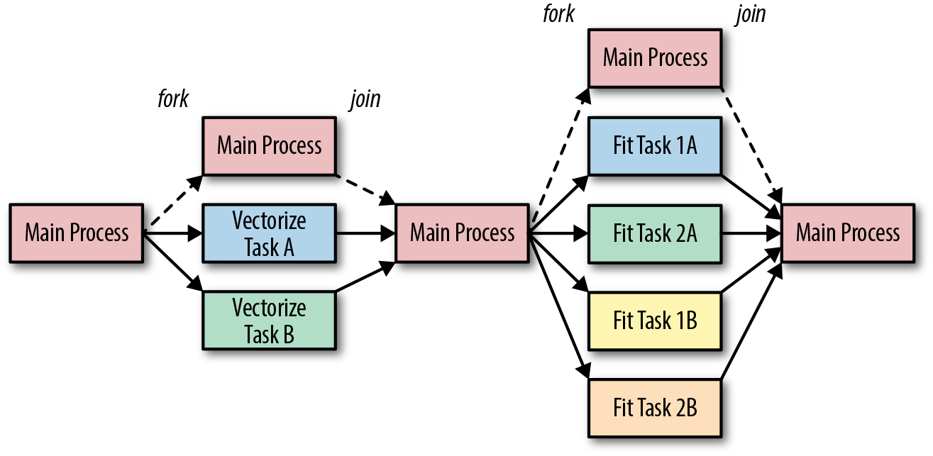
Figure 11-1. Task parallelism architecture
In the next section, we will explore how to achieve this type of task parallelism using the multiprocessing library.
Running Tasks in Parallel
In order to illustrate how multiprocessing can help us perform machine learning on text, let’s consider an example where we would like to fit multiple models, cross-validate them, and save them to disk. We will begin by writing three functions to generate a naive Bayes model, a logistic regression, and a multilayer perceptron. Each function in turn creates three different models, defined by Pipelines, that extract text from a corpus located at a specified path. Each task also determines a location to write the model to, and reports results using the logging module (more on this in a bit):
fromtransformersimportTextNormalizer,identityfromsklearn.pipelineimportPipelinefromsklearn.naive_bayesimportMultinomialNBfromsklearn.linear_modelimportLogisticRegressionfromsklearn.feature_extraction.textimportTfidfVectorizerfromsklearn.neural_networkimportMLPClassifierdeffit_naive_bayes(path,saveto=None,cv=12):model=Pipeline([('norm',TextNormalizer()),('tfidf',TfidfVectorizer(tokenizer=identity,lowercase=False)),('clf',MultinomialNB())])ifsavetoisNone:saveto="naive_bayes_{}.pkl".format(time.time())scores,delta=train_model(path,model,saveto,cv)logger.info(("naive bayes training took {:0.2f} seconds ""with an average score of {:0.3f}").format(delta,scores.mean()))deffit_logistic_regression(path,saveto=None,cv=12):model=Pipeline([('norm',TextNormalizer()),('tfidf',TfidfVectorizer(tokenizer=identity,lowercase=False)),('clf',LogisticRegression())])ifsavetoisNone:saveto="logistic_regression_{}.pkl".format(time.time())scores,delta=train_model(path,model,saveto,cv)logger.info(("logistic regression training took {:0.2f} seconds ""with an average score of {:0.3f}").format(delta,scores.mean()))deffit_multilayer_perceptron(path,saveto=None,cv=12):model=Pipeline([('norm',TextNormalizer()),('tfidf',TfidfVectorizer(tokenizer=identity,lowercase=False)),('clf',MLPClassifier(hidden_layer_sizes=(10,10),early_stopping=True))])ifsavetoisNone:saveto="multilayer_perceptron_{}.pkl".format(time.time())scores,delta=train_model(path,model,saveto,cv)logger.info(("multilayer perceptron training took {:0.2f} seconds ""with an average score of {:0.3f}").format(delta,scores.mean()))
Note
For simplicity, the pipelines for fit_naive_bayes, fit_logistic_regression, and fit_multilayer_perceptron share the first two steps, using the text normalizer and vectorizer as discussed in Chapter 4; however, you can imagine that different feature extraction methods might be better for different models.
While each of our functions can be modified and customized individually, each must also share common code. This shared functionality is defined in the train_model() function, which creates a PickledCorpusReader from the specified path. The train_model() function uses this reader to create instances and labels, compute scores using the cross_val_score utility from Scikit-Learn, fit the model, write it to disk using joblib (a specialized pickle module used by Scikit-Learn), and return the scores:
fromreaderimportPickledCorpusReaderfromsklearn.externalsimportjoblibfromsklearn.model_selectionimportcross_val_score@timeitdeftrain_model(path,model,saveto=None,cv=12):# Load the corpus data and labels for classificationcorpus=PickledCorpusReader(path)X=documents(corpus)y=labels(corpus)# Compute cross validation scoresscores=cross_val_score(model,X,y,cv=cv)# Fit the model on entire datasetmodel.fit(X,y)# Write to disk if specifiedifsaveto:joblib.dump(model,saveto)# Return scores as well as training time via decoratorreturnscores
Note
Note that our train_model function constructs the corpus reader itself (rather than being passed a reader object). When considering multiprocessing, all arguments to functions as well as return objects must be serializable using the pickle module. If we imagine that the CorpusReader is only created in the child processes, there is no need to pickle it and send it back and forth. Complex objects can be difficult to pickle, so while it is possible to pass a CorpusReader to the function, it is sometimes more efficient and simpler to pass only simple data such as strings.
The documents() and labels() are helper functions that read the data from the corpus reader into a list in memory as follows:
defdocuments(corpus):return[list(corpus.docs(fileids=fileid))forfileidincorpus.fileids()]deflabels(corpus):return[corpus.categories(fileids=fileid)[0]forfileidincorpus.fileids()]
We can keep track of the time of execution using a @timeit wrapper, a simple debugging decorator that we will use to compare performance times:
importtimefromfunctoolsimportwrapsdeftimeit(func):@wraps(func)defwrapper(*args,**kwargs):start=time.time()result=func(*args,**kwargs)returnresult,time.time()-startreturnwrapper
Python’s logging module is generally used to coordinate complex logging across multiple threads and modules. The logging configuration is at the top of the module, outside of any function, so it is executed when the code is imported. In the configuration, we can specify the %(processName)s directive, which allows us to determine which process is writing the log message. The logger is set to the module’s name so that different modules’ log statements can also be disambiguated:
importlogging# Logging configurationlogging.basicConfig(level=logging.INFO,format="%(processName)-10s%(asctime)s%(message)s",datefmt="%Y-%m-%d%H:%M:%S")logger=logging.getLogger(__name__)logger.setLevel(logging.INFO)
Note
Logging is not multiprocess-safe for writing to a single file (though it is thread-safe). Generally speaking, writing to stdout or stderr should be fine, but more complex solutions exist to manage multiprocess logging in an application context. As a result, it is a good practice to start with logging (instead of print statements) to prepare for production environment.
At long last, we’re ready to actually execute our code in parallel, with a run_parallel function. This function takes a path to the corpus as an argument, the argument that is shared by all tasks. The task list is defined, then for each function in the task list, we create an mp.Process object whose name is the name of the task, target is the callable, and args and kwargs are specified as a tuple and a dictionary, respectively. To keep track of the processes we append them to a procs list before starting the process.
At this point, if we did nothing, our main process would exit as the run_parallel function is complete, which could cause our child processes to exit prematurely or to be orphaned (i.e., never terminate). To prevent this, we loop through each of our procs and join them, rejoining each to the main process. This will cause the main function to block (wait) until the processes’ join method is called. By looping through each proc, we ensure that we don’t continue until all processes have completed, at which point we can log how much total time the process took:
defrun_parallel(path):tasks=[fit_naive_bayes,fit_logistic_regression,fit_multilayer_perceptron,]logger.info("beginning parallel tasks")start=time.time()procs=[]fortaskintasks:proc=mp.Process(name=task.__name__,target=task,args=(path,))procs.append(proc)proc.start()forprocinprocs:proc.join()delta=time.time()-startlogger.info("total parallel fit time: {:0.2f} seconds".format(delta))if__name__=='__main__':run_parallel("corpus/")
Running these three tasks in parallel requires a little extra thought and a bit more work to ensure that everything is set up correctly. So what do we get out of it? In Table 11-1, we show a comparison of task and total time averaged over ten runs.
| Task | Sequential | Parallel |
|---|---|---|
Fit Naive Bayes |
86.93 seconds |
94.18 seconds |
Fit Logistic Regression |
91.84 seconds |
100.56 seconds |
Fit Multilayer Perceptron |
95.16 seconds |
103.40 seconds |
Fit Total |
273.94 seconds |
103.47 seconds |
We can see that each individual task takes slightly longer when running in parallel; potentially, this extra time represents the minimal amount of overhead required to set up and manage multiprocessing. This slight increase in time is more than made up for in the total run time—roughly the length of the longest fit task and 2.6x times faster than running each task sequentially. When running a significant number of modeling tasks, multiprocessing clearly makes a difference!
While this use of multiprocessing.Process demonstrates a number of essential concepts, far more common is the use of a process pool, which we will discuss in the next section.
Note
It is important to keep in mind how much data is being loaded into memory, especially in a multiprocessing context. On a single machine, each process has to share memory. On a 16 GB machine, loading a 4 GB corpus in four task processes will completely consume the available memory and will slow down the overall execution. It is common to stagger task parallel execution to avoid such issues, starting longer-running tasks first, then starting up faster tasks. This can be done with delays using sleep or process pools as we’ll see in the next section.
Process Pools and Queues
In the previous section we looked at how to use the multiprocessing.Process object to run individual tasks in parallel. The Process object makes it easy to define individual functions to run independently, closing the function when it is complete. More advanced usage might employ subclasses of the Process object, each of which must implement a run() method that defines their behavior.
In larger architectures this allows easier management of individual processes and their arguments (e.g., naming them independently or managing database connections or other per-process attributes) and is generally used for task parallel execution. With task parallelism, each task has independent input and output (or the output of one task may be the input to another task). In contrast, data parallelism requires the same task to be mapped to multiple inputs. Because the input is independent, each task can be applied in parallel. For data parallelism, the multiprocessing library provides simpler abstractions in the form of Pools and Queues, which we’ll explore in this section.
Note
A common combination of both data and task parallelism is to have two data parallel tasks; the first maps an operation to many data inputs and the second reduces the map operation to a set of aggregations. This style of parallel computing has been made very popular by Hadoop and Spark, which we will discuss in the next section.
Larger workflows can be described as a directed acyclic graph (DAG), where a series of parallel steps is executed with synchronization points in between. A synchronization point ensures that all parts of the processing have completed or caught up before execution continues. Data is also generally exchanged at synchronization points, sent out to parallel tasks from the main task, or retrieved by the main task.
Data parallel execution is still appropriate for the Python multiprocessing library, however, some additional considerations are required. The first is how many processes to use and how. For simple operations, it is inefficient to run a process for each input and then tear the process down (or worse, run one process per input, which would swamp your operating system). Instead, a fixed number of processes is instantiated in a multiprocessing.Pool, each of which read input, apply the operation, then send output until the input data is exhausted.
This leads to the second consideration: How do you safely send and receive data from a process, ensuring no duplication or corruption? For this, you need to use a multiprocessing.Queue, a data structure that is both thread- and multiprocessing-safe because operations are synchronized with locks to ensure that only one process or thread has access to the queue at a time. A process can safely put(item) an item on the queue and another process can safely get() an item from the queue in a first-in, first-out (FIFO) fashion.
A common architecture for this type of processing is shown in Figure 11-2. The Pool forks n processes, each of which gets to work reading an input queue and sending their data to an output queue. The main process continues by enqueuing input data into the input queue. Generally once it’s done enqueuing the input data, the main process also enqueues n semaphores, flags that tell the processes in the process pool that there is no more data and they can terminate. The main process then can join the pool waiting for all processes to complete, or begin work immediately fetching data from the output queue for final processing.
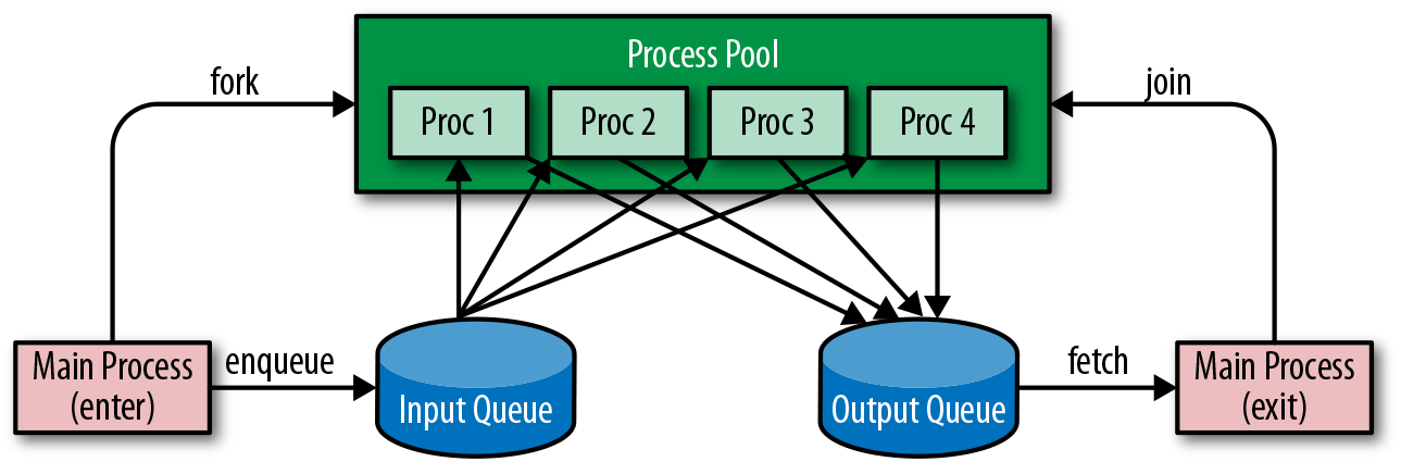
Figure 11-2. Process pool and queues
If this all sounds like a lot of work to set up each data structure and maintain the code for enqueuing and processing, don’t worry, the multiprocessing library provides simple methods on the Pool object to perform this work. The methods, apply, map, imap, and starmap each take a function and arguments and send them to the pool for processing, blocking until returning a result. These methods also have an _async counterpart—for example, apply_async does not block but instead returns an AsynchronousResult object that is filled in when the task is done, or can call callbacks on success or error when completed. We’ll see how to use apply_async in the next section.
Parallel Corpus Preprocessing
Adapting a corpus reader to use multiprocessing can be fairly straightforward when you consider that each document can be independently processed for most tasks, particularly for things like frequency analysis, vectorization, and estimation. In these cases, all multiprocessing requires is a function whose argument is a path on disk, and the fileids read from the corpus can be mapped to a process pool.
Probably the most common and time-consuming task applied to a corpus, however, is preprocessing the corpus from raw text into a computable format. Preprocessing, discussed in Chapter 3, takes a document and converts it into a standard data structure: a list of paragraphs that are lists of sentences, which in turn are lists of (token, part of speech) tuples. The final result of preprocessing is usually saving the document as a pickle, which is both usually more compact than the original document as well as easily loaded into Python for further processing.
In Chapter 3, we created a Preprocessor class that wrapped a CorpusReader object so that a method called process was applied to each document path in the corpus. The main entry point to run the preprocessor was a transform method that kicked off transforming documents from the corpus and saving them into a target directory.
Here we will extend that class, which gives us the ability to use apply_async with a callback that saves state. In this case we create a self.results list to store the results as they come back from the process() method, but it is easy to adapt on_result() to update a process or do logging.
Next, we modify the transform method to count the cores available on the local machine using mp.cpu_count(). We then create the process pool, enqueuing the tasks by iterating over all the fileids and applying them to the pool (which is where the callback functionality comes into play to modify the state). Finally we close the pool (with pool.close()), meaning that no additional tasks can be applied and the child processes will join when done, and we wait for them to complete (with pool.join()):
classParallelPreprocessor(Preprocessor):defon_result(self,result):self.results.append(result)deftransform(self,tasks=None):[...]# Reset the resultsself.results=[]# Create a multiprocessing pooltasks=tasksormp.cpu_count()pool=mp.Pool(processes=tasks)# Enqueue tasks on the multiprocessing pool and joinforfileidinself.fileids():pool.apply_async(self.process,(fileid,),callback=self.on_result)# Close the pool and joinpool.close()pool.join()returnself.results
Note
The results of multiprocessing are significant. Anecdotally, on a subset of the Baleen corpus, which consisted of about 1.5 million documents, serial processing took approximately 30 hours—a rate of about 13 documents per second. Using a combination of task and data parallelism with 16 workers, the preprocessing task was reduced to under 2 hours.
Although this introduction to threads and multiprocessing was brief and high-level hopefully it gives you a sense of the challenges and opportunities provided by parallelism. Many text analysis tasks can be sped up and scaled linearly simply by using the multiprocessing module and applying already existing code. By running multiprocessing code on a modern laptop or by using a large compute-optimized cloud instance, it is relatively simple to take advantage of multiprocessing without the overhead of setting up a cluster. Compared to cluster computations, programs written with multiprocessing are also easier to reason about and manage.
Cluster Computing with Spark
Multiprocessing is a simple and effective way to take advantage of today’s multicore commercial hardware; however, as processing jobs get larger, there is a physical and economic limit to the number of cores available on a single machine. At some point buying a machine with twice the number of cores becomes more expensive than buying two machines to get the same number of processors. This simple motivation has ushered in a new wave of particularly accessible cluster computing methodologies.
Cluster computing concerns the coordination of many individual machines connected together by a network in a consistent and fault-tolerant manner—for example, if a single machine fails (which becomes more likely when there are many machines), the entire cluster does not fail. Unlike the multiprocessing context, there is no single operating system scheduling access to resources and data. Instead, a framework is required to manage distributed data storage, the storage and replication of data across many nodes, and distributed computation, the coordination of computation tasks across networked computers.
Note
While beyond the scope of this book, distributed data storage is a necessary preliminary step before any cluster computation can take place if you want the cluster computation to happen reliably. Generally, cluster filesystems like HDFS or S3 and databases like Cassandra and HBase are used to manage data on disk.
In the rest of the chapter, we will explore the use of Apache Spark as a distributed computation framework for text analysis tasks. Our treatment serves only as a brief introduction and does not go into the depth required of such a large topic. We leave installation of Spark and PySpark to the reader, though detailed information can be found in the Spark documentation.2 For a more comprehensive introduction, we recommend Data Analytics with Hadoop (O’Reilly).3
Anatomy of a Spark Job
Spark is an execution engine for distributed programs whose primary advantage is support for in-memory computing. Because Spark applications can be written quickly in Java, Scala, Python, and R it has become synonymous with Big Data science. Several libraries built on top of Spark such as Spark SQL and DataFrames, MLlib, and GraphX mean that data scientists used to local computing in notebooks with these tools feel comfortable very quickly in the cluster context. Spark has allowed applications to be developed upon datasets previously inaccessible to machine learning due to their scope or size; a category that many text corpora fall into. In fact, cluster computing frameworks were originally developed to handle text data scraped from the web.
Spark can run in two modes: client mode and cluster mode. In cluster mode, a job is submitted to the cluster, which then computes independently. In client mode, a local client connects to the cluster in an interactive fashion; jobs are sent to the cluster and the client waits until the job is complete and data is returned. This makes it possible to interact with the cluster using PySpark, an interactive interpreter similar to the Python shell, or in a Juypter notebook. For dynamic analysis, client mode is perfect for quickly getting answers to questions on smaller datasets and corpora. For more routine or longer running jobs, cluster mode is ideal.
In this section we will briefly explore how to compose Python programs using Spark’s version 2.x API. The code can be run locally in PySpark or with the spark-submit command.
With PySpark:
$ pyspark
Python 3.6.3 (v3.6.3:2c5fed86e0, Oct  3 2017, 00:32:08)
[GCC 4.2.1 (Apple Inc. build 5666) (dot 3)] on darwin
Type "help", "copyright", "credits" or "license" for more information.
Welcome to
      ____              __
     / __/__  ___ _____/ /__
    _\ \/ _ \/ _ `/ __/  '_/
   /__ / .__/\_,_/_/ /_/\_\   version 2.3.0
      /_/

Using Python version 3.6.3 (v3.6.3:2c5fed86e0, Oct  3 2017 00:32:08)
SparkSession available as 'spark'.
>>> import hello
With spark-submit:
$ spark-submit hello.pyIn practice we would use a series of flags and arguments in the above spark-submit command to let Spark know, for example, the URL for the cluster (with --master), the entry point for the application (with --class), the location for the driver to execute in the deployment environment (with --deploy-mode), etc.
A connection to the cluster, called the SparkContext, is required. Generally, the SparkContext is stored in a global variable, sc, and if you launch PySpark in either a notebook or a terminal, the variable will immediately be available to you. If you run Spark locally, the SparkContext is essentially what gives you access to the Spark execution environment, whether that’s a cluster or a single machine. To create a standalone Python job, creating the SparkContext is the first step, and a general template for Spark jobs is as follows:
frompysparkimportSparkConf,SparkContextAPP_NAME="My Spark Application"defmain(sc):# Define RDDs and apply operations and actions to them.if__name__=="__main__":# Configure Sparkconf=SparkConf().setAppName(APP_NAME)sc=SparkContext(conf=conf)# Execute Main functionalitymain(sc)
Now that we have a basic template for running Spark jobs, the next step is to load data from disk in a way that Spark can use, as we will explore in the next section.
Distributing the Corpus
Spark jobs are often described as directed acyclic graphs (DAGs), or as acyclic data flows. This refers to a style of programming that envisions data loaded into one or more partitions, and subsequently transformed, merged, or split until some final state is reached. As such, Spark jobs begin with resilient distributed datasets (RDDs), collections of data partitioned across multiple machines, which allows safe operations to be applied in a distributed manner.
The simplest way to create RDDs is to organize data similarly to how we organized our corpus on disk—directories with document labels, and each document as its own file on disk. For example, to load the hobbies corpus introduced in “Loading Yellowbrick Datasets”, we use sc.wholeTextFiles to return an RDD of (filename, content) pairs. The argument to this method is a path that can contain wildcards and point to a directory of files, a single file, or compressed files. In this case, the syntax "hobbies/*/*.txt" looks for any file with a .txt extension under any directory in the hobbies directory:
corpus=sc.wholeTextFiles("hobbies/*/*.txt")(corpus.take(1))
The take(1) action prints the first element in the corpus RDD, allowing you to visualize that the corpus is a collection of tuples of strings. With the hobbies corpus, the first element shows as follows:
[('file:/hobbies/books/56d62a53c1808113ffb87f1f.txt',
"\r\n\r\nFrom \n\n to \n\n, Oscar voters can't get enough of book
adaptations. Nowhere is this trend more obvious than in the Best
Actor and Best Actress categories.\n\n\r\n\r\nYes, movies have
been based on books and true stories since the silent film era,
but this year represents a notable spike...")]
Saving data to disk and parsing it can be applied to a variety of formats including other text formats like JSON, CSV, and XML or binary formats like Avro, Parquet, Pickle, Protocol Buffers, etc., which can be more space-efficient. Regardless, once preprocessing has been applied (either with Spark or as described in “Parallel Corpus Preprocessing”), data can be stored as Python objects using the RDD.saveAsPickleFile method (similar to how we stored pickle files for our preprocessed corpus) and then loaded using sc.pickleFile.
Now that we’ve loaded our hobbies corpus into RDDs, the next step is to apply transformations and actions to them, which we will discuss more in the next section.
RDD Operations
There are two primary types of operations in a Spark program: transformations and actions. Transformations are operations that manipulate data, creating a new RDD from an existing one. Transformations do not immediately cause execution to occur on the cluster, instead they are described as a series of steps applied to one or more RDDs. Actions, on the other hand, do cause execution to occur on the cluster, causing a result to be returned to the driver program (in client mode) or data to be written to disk or evaluated in some other fashion (in cluster mode).
Caution
Transformations are evaluated lazily, meaning they are applied only when an action requires a computed result, which allows Spark to optimize how RDDs are created and stored in memory. For users, this can cause gotchas; at times exceptions occur and it is not obvious which operation caused them; other times an action causes a very long running procedure to be sent to the cluster. Our rule of thumb is to develop in client mode on a sample of the total dataset, then create applications that are submitted in cluster mode.
The three most common transformations—map, filter, and flatMap—each accept a function as their primary argument. This function is applied to each element in the RDD and each returned value is used to create the new RDD.
For instance, we can use the Python operator module to extract the hobbies subcategory for each document. We create a parse_label function that can extract the category name from the document’s filepath. As in the example we looked at before, the data RDD of (filename, content) key-value pairs is created by loading whole text files from the specified corpus path. We can then create the labels RDD by mapping itemgetter(0), an operation that selects only filenames from each element of the data RDD, then mapping the parse_label function to each:
importosfromoperatorimportitemgetterdefparse_label(path):# Returns the name of the directory containing the filereturnos.path.basename(os.path.dirname(path))data=sc.wholeTextFiles("hobbies/*/*.txt")labels=data.map(itemgetter(0)).map(parse_label)
Note that at this point, nothing is executed across the cluster because we’ve only defined transformations, not actions. Let’s say we want to get the count of the documents in each of the subcategories.
While our labels RDD is currently a collection of strings, many Spark operations (e.g., groupByKey and reduceByKey) work only on key-value pairs. We can create a new RDD called label_counts, which is first transformed by mapping each label into a key-value pair, where the key is the label name, and the value is a 1. We can then reduceByKey with the add operator, which will sum all the 1s by key, giving us the total count of documents per category. We then use the collect action to execute the transformations across the cluster, loading the data, creating the labels and label_count RDD, and returning a list of (label, count), tuples, which can be printed in the client program:
fromoperatorimportaddlabel_count=labels.map(lambdal:(l,1)).reduceByKey(add)forlabel,countinlabel_count.collect():("{}: {}".format(label,count))
The result is as follows:
books: 72
cinema: 100
gaming: 128
sports: 118
cooking: 30
Note
Other actions include reduce (which aggregates elements of the collection), count (which returns the number of elements in the collection), and take and first (which return the first item or the first n items from the collection, respectively). These actions are useful in interactive mode and debugging, but take care when working with big RDDs—it can be easy to try to load a large dataset into the memory of a machine that can’t store it! More common with big datasets is to use takeSample, which performs a random uniform sample with or without replacement on the collection, or to simply save the resulting dataset back to disk to be operated on later.
As we’ve discussed in previous sections, Spark applications are defined by data flow operations. We first load data into one or more RDDs, apply transformations to those RDDs, join and merge them, then apply actions and save the resulting data to disk or aggregate data and bring it back to a driver program. This is a powerful abstraction that allows us to think about data as a collection rather than as a distributed computation, enabling cluster computing without requiring much effort on the analyst’s part. More complex usage of Spark involves creating DataFrames and Graphs, a little of which we’ll see in the next section.
NLP with Spark
Natural language processing is a special interest of the distributed systems community. This is not only because some of the largest datasets are text (in fact, Hadoop was designed specifically to parse HTML documents for search engines), but also because cutting-edge, language-aware applications require especially large corpora to be effective. As a result, Spark’s machine learning library, MLLib,4 boasts many tools for intelligent feature extraction and vectorization of text similar to the ones discussed in Chapter 4, including utilities for frequency, one-hot, TF–IDF, and word2vec encoding.
Machine learning with Spark starts with a collection of data similar to an RDD, the SparkSQL DataFrame. Spark DataFrames are conceptually equivalent to relational database tables or their Pandas counterparts, coordinating data by row and column as a table. However, they add rich optimizations that take advantage of the SparkSQL execution engine, and are quickly becoming the standard for distributed data science.
If we wanted to use SparkMLLib on our hobbies corpus, we would first transform the corpus RDD using a SparkSession (exposed as the global variable spark in PySpark) to create a DataFrame from the collection of tuples, identifying each column by name:
# Load data from diskcorpus=sc.wholeTextFiles("hobbies/*/*.txt")# Parse the label from the text pathcorpus=corpus.map(lambdad:(parse_label(d[0]),d[1]))# Create the dataframe with two columnsdf=spark.createDataFrame(corpus,["category","text"])
The SparkSession is the entry point to SparkSQL and the Spark 2.x API. To use this in a spark-submit application, you must first build it, similar to how we constructed the the SparkContext in the previous section. Adapt the Spark program template by adding the following lines of code:
frompyspark.sqlimportSparkSessionfrompysparkimportSparkConf,SparkContextAPP_NAME="My Spark Text Analysis"defmain(sc,spark):# Define DataFrames and apply ML estimators and transformersif__name__=="__main__":# Configure Sparkconf=SparkConf().setAppName(APP_NAME)sc=SparkContext(conf=conf)# Build SparkSQL Sessionspark=SparkSession(sc)# Execute Main functionalitymain(sc,spark)
With our corpus structured as a Spark DataFrame, we can now get to the business of fitting models and transforming datasets. Luckily, Spark’s API is very similar to the Scikit-Learn API, so transitioning from Scikit-Learn or using Scikit-Learn and Spark in conjunction is not difficult.
From Scikit-Learn to MLLib
Spark’s MLLib has been rapidly growing and includes estimators for classification, regression, clustering, collaborative filtering, and pattern mining. Many of these implementations are inspired by Scikit-Learn estimators, and for Scikit-Learn users, MLLib’s API and available models will be instantly recognizable.
However, it is important to remember that Spark’s core purpose is to perform computations on extremely large datasets in a cluster. It does so using optimizations in distributed computation. This means that easily parallelized algorithms are likely to be available in MLLib, while others that are not easily constructed in a parallel fashion, may not. For example, Random Forest involves randomly splitting the dataset and fitting decision trees on subsets of the data that can easily be partitioned across machines. Stochastic gradient descent, on the other hand, is very difficult to parallelize because it updates after each iteration. Spark chooses strategies to optimize cluster computing, not necessarily the underlying model. For Scikit-Learn users, this may manifest in less accurate models (due to Spark’s approximations) or fewer hyperparameter options. Other models (e.g., k-nearest neighbor) may simply be unavailable because they cannot be effectively distributed.
Like Scikit-Learn, the Spark ML API centers around the concept of a Pipeline. Pipelines allow a sequence of algorithms to be constructed together so as to represent a single model that can learn from data and produce estimations in return.
Note
In Spark, unlike Scikit-Learn, fitting an estimator or pipeline returns a completely new model object instead of simply modifying the internal state of the estimator. The reason for this is that RDDs are immutable.
Spark’s Pipeline object is composed of stages, and each of these stages must be either a Transformer or an Estimator. Transformers convert one DataFrame into another by reading a column from the input DataFrame, mapping it to a transform() method, and appending a new column to the Dataframe. This means that all transformers generally need to specify the input and output column names, which must be unique.
Estimators implement a fit() method, which learns from data and then returns a new model. Models are themselves transformers, so estimators also define input and output columns on the DataFrame. When a predictive model calls transform(), the estimations or predictions are stored in the output column. This is slightly different from the Scikit-Learn API, which has a predict() method, but the transform() method is more appropriate in a distributed context since it is being applied to a potentially very large dataset.
Caution
Pipeline stages must be unique to ensure compile-time checking and an acyclic graph, which is the graph of transformations and actions in the underlying spark execution. This means that inputCol and outputCol parameters must be unique in each stage and that an instance cannot be used twice as different stages.
Because model storage and reuse is critical to the machine learning workflow, Spark can also export and import models on demand. Many Transformer and Pipeline objects have a save() method to export the model to disk and an associated load() method to load the saved model.
Finally, Spark’s MLLib contains one additional concept: the Parameter. Parameters are distributed data structures (objects) with self-contained documentation. Such a data structure is required for machine learning because these variables must be broadcast to all executors in the cluster in a safe manner. Broadcast variables are read-only data that is pickled and available as a global in each executor in the cluster.
Some parameters may even be updated during the fit process, requiring accumulation. Accumulators are distributed data structures that can have associative and commutative operations applied to them in a parallel-safe manner. Therefore, many parameters must be retrieved or set using special Transformer methods, the most generic of which are getParam(param), getOrDefault(param), and setParams(). It is possible to view a parameter and its associated values with the explainParam() method, a useful and routinely used utility in PySpark and Jupyter notebooks.
Now that we have a basic understanding of the Spark MLLib API, we can explore some examples in detail in the next section.
Feature extraction
The first step to natural language processing with Spark is extracting features from text, tokenizing and vectorizing utterances and documents. Spark provides a rich toolset of feature extraction methodologies for text including indexing, stopwords removal, and n-gram features. Spark also provides vectorization utilities for frequency, one-hot, TF–IDF, and Word2Vec encoding. All of these utilities expect input as a list of tokens, so the first step is generally to apply tokenization.
In the following snippet, we initialize a Spark RegexTokenizer transformer with several parameters. The inputCol and outputCol parameters specify how transformers will work on the given DataFrame; the regular expression, "\\w+", specifies how to chunk text; and gaps=False ensures this pattern will match words instead of matching the space between words. When the corpus DataFrame (here we assume the corpus has already been loaded) is transformed, it will contain a new column, “tokens,” whose data type is an array of strings, the data type required for most other feature extraction:
frompyspark.ml.featureimportRegexTokenizer# Create the RegexTokenizertokens=RegexTokenizer(inputCol="text",outputCol="tokens",pattern="\\w+",gaps=False,toLowercase=True)# Transform the corpuscorpus=tokens.transform(corpus)
This tokenizer will remove all punctuation and split hyphenated words. A more complex pattern such as "\\w+|\$[\\d\.]+|\\S+" will split punctuation but not remove it and even capture money expressions such as "$8.31".
Caution
Occasionally Spark models will have defaults for inputCol and outputCol, such as "features" or "predictions", which can lead to errors or incorrect workflows; generally it is best to specify these parameters specifically on each transformer and model.
Because converting documents to feature vectors involves multiple steps that need to be coordinated together, vectorization is composed as a Pipeline. Creating local variables for each transformer and then putting them together into a Pipeline is very common but can make Spark scripts verbose and prone to user error. One solution to this is to define a function that can be imported into your script that returns a Pipeline of standard vectorization for your corpus.
The make_vectorizer function creates a Pipeline with a Tokenizer and a HashingTF vectorizer to map tokens to their term frequencies using the hashing trick, which computes the Murmur3 hash of the token and uses that as the numeric feature. This function can also add stopwords removal and TF–IDF transformers to the Pipeline on demand. In order to ensure that the DataFrame is being transformed with unique columns, each transformer assigns a unique output column name and uses stages[-1].getOutputCol() to determine the input column name from the stage before:
defmake_vectorizer(stopwords=True,tfidf=True,n_features=5000):# Creates a vectorization pipeline that starts with tokenizationstages=[Tokenizer(inputCol="text",outputCol="tokens"),]# Append stopwords to the pipeline if requestedifstopwords:stages.append(StopWordsRemover(caseSensitive=False,outputCol="filtered_tokens",inputCol=stages[-1].getOutputCol(),),)# Create the Hashing term frequency vectorizerstages.append(HashingTF(numFeatures=n_features,inputCol=stages[-1].getOutputCol(),outputCol="frequency"))# Append the IDF vectorizer if requestediftfidf:stages.append(IDF(inputCol=stages[-1].getOutputCol(),outputCol="tfidf"))# Return the completed pipelinereturnPipeline(stages=stages)
Because of the HashingTF and IDF models, this vectorizer needs to be fit on input data; make_vectorizer().fit(corpus) ensures that vectors will be a model that is able to perform transformations on the data:
vectors=make_vectorizer().fit(corpus)corpus=vectors.transform(corpus)corpus[['label','tokens','tfidf']].show(5)
The first five rows of the result are as follows:
+-----+--------------------+--------------------+
|label|              tokens|               tfidf|
+-----+--------------------+--------------------+
|books|[, name, :, ian, ...|(5000,[15,24,40,4...|
|books|[, written, by, k...|(5000,[8,177,282,...|
|books|[, last, night,as...|(5000,[3,9,13,27,...|
|books|[, a, sophisticat...|(5000,[26,119,154...|
|books|[, pools, are, so...|(5000,[384,569,60...|
+------+--------------------+--------------------+
only showing top 5 rows
Once the corpus is transformed it will contain six columns, the two original columns, and the four columns representing each step in the transformation process; we can select three for inspection and debugging using the DataFrame API.
Now that our features have been extracted, we can begin to create models and engage the model selection triple, first with clustering and then with classification.
Text clustering with MLLib
At the time of this writing, Spark implements four clustering techniques that are well suited to topic modeling: k-means and bisecting k-means, Latent Dirichlet Allocation (LDA), and Gaussian mixture models (GMM). In this section, we will demonstrate a clustering pipeline that first uses Word2Vec to transform the bag-of-words into a fixed-length vector, and then BisectingKMeans to generate clusters of similar documents.
Bisecting k-means is a top-down approach to hierarchical clustering that uses k-means to recursively bisect clusters (e.g., k-means is applied to each cluster in the hierarchy with k=2). After the cluster is bisected, the split with the highest overall similarity is reserved, while the remaining data continues to be bisected until the desired number of clusters is reached. This method converges quickly and because it employs several iterations of k=2 it is generally faster than k-means with a larger k, but it will create very different clusters than the base k-means algorithm alone.
In the code snippet, we create an initial Pipeline that defines our input and output columns as well as the parameters for our transformers, such as the fixed size of the word vectors and the k for k-means. When we call fit on our data, our Pipeline will produce a model, which can then in turn be used to transform the corpus:
fromtabulateimporttabulatefrompyspark.mlimportPipelinefrompyspark.ml.clusteringimportBisectingKMeansfrompyspark.ml.featureimportWord2Vec,Tokenizer# Create the vector/cluster pipelinepipeline=Pipeline(stages=[Tokenizer(inputCol="text",outputCol="tokens"),Word2Vec(vectorSize=7,minCount=0,inputCol="tokens",outputCol="vecs"),BisectingKMeans(k=10,featuresCol="vecs",maxIter=10),])# Fit the modelmodel=pipeline.fit(corpus)corpus=model.transform(corpus)
To evaluate the success of our cluster, we must first retrieve the BisectingKMeans and Word2Vec objects and store them in local variables: bkm by accessing the last stage of the model (not the Pipeline) and wvec the penultimate stage. We use the computeCost method to compute the sum of square distances to the assigned center of each document (here, again, we assume corpus documents have already been loaded). The smaller the cost, the tighter and more defined the clusters we have. We can also compute the size in number of documents each cluster is composed of:
# Retrieve stagesbkm=model.stages[-1]wvec=model.stages[-2]# Evaluate clusteringcost=bkm.computeCost(corpus)sizes=bkm.summary.clusterSizes
To get a text representation of each center, we first must loop through every cluster index (ci) and cluster centroid (c) by enumerating the cluster centers. For each center we can find the seven closest synonyms, the word vectors that are closest to the center, then construct a table that displays the center index, the size of the cluster, and the associated synonyms. We can then pretty-print the table with the tabulate library:
# Get the text representation of each clustertable=[["Cluster","Size","Terms"]]forci,cinenumerate(bkm.clusterCenters()):ct=wvec.findSynonyms(c,7)size=sizes[ci]terms=" ".join([row.wordforrowinct.take(7)])table.append([ci,size,terms])# Print the results(tabulate(table))("Sum of square distance to center: {:0.3f}".format(cost))
With the following results:
Cluster  Size  Terms
-------  ----  ---------------------------------------------------------------
    0      81  the"soros caption,"bye markus henkes clarity. presentation,elon
    1       3  novak hiatt  veered monopolists,then,would clarity. cilantro.
    2       2  publics. shipmatrix. shiri flickr groupon,meanwhile,has sleek!
    3       2  barrymore 8,2016 tips? muck glorifies tags between,earning
    4     265  getting sander countervailing officers,ohio,then voter. dykstra
    5     550  back peyton's condescending embryos racist,any voter. nebraska
    6     248  maxx,and davan think'i smile,i 2014,psychologists thriving.
    7     431  ethnography akhtar problem,and studies,taken monica,california.
    8     453  instilled wife! pnas,the ideology,with prowess,pride
    9     503  products,whereas attacking grouper sets,facebook flushing,
Sum of square distance to center: 39.750
We can see that some of our clusters appear to be very large and diffuse, so our next steps would be to perform evaluations as discussed in Chapters 6 and 8 to modify k until a suitable model is achieved.
Text classification with MLLib
Spark’s classification library currently includes models for logistic regression, decision trees, random forest, gradient boosting, multilayer perceptrons, and SVMs. These models are well suited for text analysis and commonly used for text classification. Classification will work similarly to clustering, but with the added steps of having to index labels for each document, as well as applying an evaluation step that computes the accuracy of the model. Because the evaluation should be made on test data that the model was not trained on, we need to split our corpus into train and test splits.
After the vectorization step, we’ll encode the document labels using StringIndexer, which will convert our DataFrame column of strings into a column of indices in [0, len(column)], ordered by frequency (e.g., the most common label will receive index 0). We can then split the DataFrame into random splits, the training data composed of 80% of the dataset and the test data composed of 20%:
frompyspark.ml.featureimportStringIndexer# Create the vectorizervector=make_vectorizer().fit(corpus)# Index the labels of the classificationlabelIndex=StringIndexer(inputCol="label",outputCol="indexedLabel")labelIndex=labelIndex.fit(corpus)# Split the data into training and test setstraining,test=corpus.randomSplit([0.8,0.2])
Note
In the preceding snippet, both the vector and labelIndex transformers were fit on all of the data before the split to ensure that all indices and terms are encoded. This may or may not be the right strategy for real models depending on your expectations of real data.
We can now create a Pipeline to construct a label and document encoding process preliminary to a LogisticRegression model:
frompyspark.ml.classificationimportLogisticRegressionmodel=Pipeline(stages=[vector,labelIndex,clf]).fit(training)# Make predictionspredictions=model.transform(test)predictions.select("prediction","indexedLabel","tfidf").show(5)
If we wanted to evaluate the model, we would next use Spark’s classification evaluation utilities. For example:
frompyspark.ml.evaluationimportMulticlassClassificationEvaluatorevaluator=MulticlassClassificationEvaluator(labelCol="indexedLabel",predictionCol="prediction",metricName="f1")score=evaluator.evaluate(predictions)("F1 Score: {:0.3f}".format(score))
Spark has other utilities for cross-validation and model selection, though these utilities are aware of the fact that models are trained on large datasets. Generally speaking, splitting large corpora and training models multiple times to get an aggregate score takes a long time on the corpus, so cacheing and active training are important parts of the modeling process to minimize duplicated workload. Understanding the trade-offs when using a distributed approach to machine learning brings us to our next topic—employing local computations across the global dataset.
Local fit, global evaluation
If you have been running the Spark code snippets locally using PySpark or spark-submit you may have noticed that Spark doesn’t seem blazingly fast as advertised; indeed it was probably slower than the equivalent modeling with Scikit-Learn on your local machine. Spark has a large overhead, creating processes that monitor jobs and perform a lot of communication between processes to synchronize them and ensure fault tolerance; the speed becomes clear when datasets are much larger than those that can be stored on a single computer.
One way to deal with this is to perform the data preprocessing and vectorization in parallel on the cluster, take a sample of the data, fit it locally, and then evaluate it globally across the entire dataset. Although this reduces the advantage of training models on large datasets, it is often the only way to produce narrow or specialized models on a cluster. This technique can be used to produce different models for different parts of the dataset or to rapidly iterate in the testing process.
First, we vectorize our corpus, then take a sample. By ensuring the vectorization occurs on the cluster, we can be assured that the Scikit-Learn model we employ will not be dependent on terms or other states that may be excluded by the sampling process. The sample is conducted without replacement (the first False argument) and gathers 10% of the data (the 0.1 argument). Be careful when choosing a size of the data to sample; you could easily bring in too much data into memory even with only 10% of the corpus! The collect() action executes the sampling code, then brings the dataset into memory on the local machine as a list. We can then construct X and y from the returned data and fit our model:
# Vectorize the corpus on the clustervector=make_vectorizer().fit(corpus)corpus=vector.transform(corpus)# Get the sample from the datasetsample=corpus.sample(False,0.1).collect()X=[row['tfidf']forrowinsample]y=[row['label']forrowinsample]# Train a Scikit-Learn Modelclf=AdaBoostClassifier()clf.fit(X,y)
To evaluate our model we will broadcast it to the cluster, and to compute accuracy, we will use one accumulator to compute the number of predictions and another to compute the incorrect ones:
# Broadcast the Scikit-Learn Model to the clusterclf=sc.broadcast(clf)# Create accumulators for correct vs incorrectcorrect=sc.accumulator(0)incorrect=sc.accumulator(1)
To use these variables in parallel execution we need a way to reference them into the DataFrame operations. In Spark, we do this by sending a closure. One common strategy to do this is to define a function that returns a closure on demand. We can define an accuracy closure that applies the predict method of the classifier to the data, then increments the correct or incorrect accumulators by comparing the predicted answer with the actual label. To create this closure we define the make_accuracy_closure function as follows:
defmake_accuracy_closure(model,correct,incorrect):# model should be a broadcast variable# correct and incorrect should be accumulatorsdefinner(rows):X=[]y=[]forrowinrows:X.append(row['tfidf'])y.append(row['label'])yp=model.value.predict(X)foryi,ypiinzip(y,yp):ifyi==ypi:correct.add(1)else:incorrect.add(1)returninner
We can then use foreachPartition action on the corpus DataFrame to have each executor send their portion of the DataFrame into the accuracy closure, which updates our accumulators. Once complete we can compute the accuracy of the model against the global dataset:
# Create the accuracy closureaccuracy=make_accuracy_closure(clf,incorrect,correct)# Compute the number incorrect and correctcorpus.foreachPartition(accuracy)accuracy=float(correct.value)/float(correct.value+incorrect.value)("Global accuracy of model was {}".format(accuracy))
The strategy of fitting locally and evaluating globally actually allows developers to easily construct and evaluate multiple models in parallel and can improve the speed of the Spark workflow, particularly during the investigation and experiment phases. Multiple models can be more easily cross-validated on medium-sized datasets, and models with partial distributed implementations (or no implementation at all) can be more fully investigated.
This is a generalization of the “last mile computing” strategy that is typical with big data systems. Spark allows you to access huge amounts of data in a timely fashion, but to make use of that data, cluster operations are generally about filtering, aggregating, or summarizing data into context, bringing it into a form that can fit into the memory of a local machine (using cloud computing resources, this can be dozens or even hundreds of gigabytes). This is one of the reasons that the interactive model of Spark execution is so favored by data scientists; it easily allows a combination of local and cluster computing as demonstrated in this section.
Conclusion
One of the best things about conducting text analysis in the information age is how easy it is to create virtuous cycles of applications that use text analysis and then generate more text data from human responses. This means that machine learning corpora quickly grow beyond what is practical to compute on in a single process or even a single machine. As the amount of time to conduct an analysis increases, the productivity of iterative or experimental workflows decreases—some method of scaling must be employed to maintain momentum.
The multiprocessing module is the first step to scaling analytics. In this case, code already employed for analysis simply has to be adapted or included in a multiprocessing context. The multiprocessing library takes advantage of multicore processors and the large amounts of memory available on modern machines to execute code simultaneously. Data is still stored locally, but with a beefy enough machine, huge amounts of work can be shortened to manageable chunks.
When the size of the data grows large enough to no longer fit on a single machine, cluster computing methodologies must be used. Spark provides an execution framework that allows for interactive computing between a local computer running PySpark in a Jupyter notebook and the cluster that runs many executors that operate on a partition of the data. This interactivity combines the best of both worlds of sequential and parallel computing algorithms. While working with Spark does require a change in the code and programming context and may even necessitate the choice of other machine learning libraries, the advantage is that large datasets that would otherwise be unavailable to text analytics techniques can become a rich fabric for novel applications.
The key to working with distributed computation is making sure the trade-offs are well understood. Understanding whether an operation is compute or I/O bound can save many headaches diagnosing why jobs are taking longer than they should or using way too many resources (and help us balance task and data parallelism). Moreover, parallel execution takes additional overhead, which must be worth the cost; understanding this helps us make decisions that enhance experimental development without getting in the way. Finally, recognizing how algorithms are approximated in a distributed context is important to building meaningful models and interpreting the results.
Spark is the first in a wave of modern technologies that are allowing us to handle more and more data to create meaningful models. In the next chapter we will explore distributed techniques for training so-called deep models—neural networks with multiple hidden layers.
1 Gene M. Amdahl, Validity of the single processor approach to achieving large scale computing capabilities, (1967) http://bit.ly/2GQKWza
2 The Apache Software Foundation, Apache Spark: Lightning-fast cluster computing, (2018) http://bit.ly/2GKR6k1
3 Benjamin Bengfort and Jenny Kim, Data Analytics with Hadoop: An Introduction for Data Scientists, (2016) https://oreil.ly/2JHfi8V
4 The Apache Software Foundation, MLlib: Apache Spark’s scalable machine learning library, (2018) http://bit.ly/2GJQP0Y