Table of Contents for
Applied Text Analysis with Python
 Applied Text Analysis with Python
Published by
O'Reilly Media, Inc., 2018
Applied Text Analysis with Python
Published by
O'Reilly Media, Inc., 2018
- Cover
- nav
- Applied Text Analysis with Python
- Applied Text Analysis with Python
- Preface
- 1. Language and Computation
- 2. Building a Custom Corpus
- 3. Corpus Preprocessing and Wrangling
- 4. Text Vectorization and Transformation Pipelines
- 5. Classification for Text Analysis
- 6. Clustering for Text Similarity
- 7. Context-Aware Text Analysis
- 8. Text Visualization
- 9. Graph Analysis of Text
- 10. Chatbots
- 11. Scaling Text Analytics with Multiprocessing and Spark
- 12. Deep Learning and Beyond
- Glossary
- Index
- About the Authors
- Colophon
Chapter 6. Clustering for Text Similarity
What would you do if you were handed a pile of papers—receipts, emails, travel itineraries, meeting minutes—and asked to summarize their contents? One strategy might be to read through each of the documents, highlighting the terms or phrases most relevant to each, and then sort them all into piles. If one pile started getting too big, you might split it into two smaller piles. Once you’d gone through all the documents and grouped them, you could examine each pile more closely. Perhaps you would use the main phrases or words from each pile to write up the summaries and give each a unique name—the topic of the pile.
This is, in fact, a task practiced in many disciplines, from medicine to law. At its core, this sorting task relies on our ability to compare two documents and determine their similarity. Documents that are similar to each other are grouped together and the resulting groups broadly describe the overall themes, topics, and patterns inside the corpus. Those patterns can be discrete (e.g., when the groups don’t overlap at all) or fuzzy (e.g., when there is a lot of similarity and documents are hard to distinguish). In either case, the resultant groups represent a model of the contents of all documents, and new documents can be easily assigned to one group or another.
While most document sorting is currently done manually, it is possible to achieve these tasks in a fraction of the time with the effective integration of unsupervised learning, as we’ll see in this chapter.
Unsupervised Learning on Text
Unsupervised approaches can be incredibly useful for exploratory text analysis. Oftentimes corpora do not arrive pretagged with labels ready for classification. In these cases, the only choice (aside from paying someone to label your data), or at least a necessary precursor for many natural language processing tasks, is an unsupervised approach.
Clustering algorithms aim to discover latent structure or themes in unlabeled data using features to organize instances into meaningfully dissimilar groups. With text data, each instance is a single document or utterance, and the features are its tokens, vocabulary, structure, metadata, etc.
In Chapter 5 we constructed our classification pipeline to compare and score many different models and select the most performant for use in predicting on new data. The behavior of unsupervised learning methods is fundamentally different; instead of learning a predefined pattern, the model attempts to find relevant patterns a priori.
As such, the integration of these techniques into a data product architecture is necessarily a bit different. As we see in the pipeline presented in Figure 6-1, a corpus is transformed into feature vectors and a clustering algorithm is employed to create groups or topic clusters, using a distance metric such that documents that are closer together in feature space are more similar. New incoming documents can then be vectorized and assigned to the nearest cluster. Later in this chapter, we’ll employ this pipeline to conduct an end-to-end clustering analysis on a sample of the Baleen corpus introduced in Chapter 2.
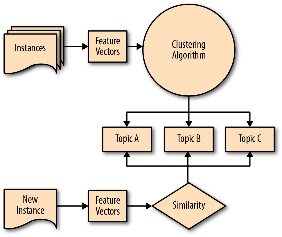
Figure 6-1. Clustering pipeline
First, we need a method for defining document similarity, and in the next section, we’ll explore a range of distance metrics that can be used in determining the relative similarity between two given documents. Next, we will explore the two primary approaches to unsupervised learning, partitive clustering and hierarchical clustering, using methods implemented in NLTK and Scikit-Learn. With the resulting clusters, we’ll experiment with using Gensim for topic modeling to describe and summarize our clusters. Finally, we will move on to exploring two alternative means of unsupervised learning for text: matrix factorization and Latent Dirichlet Allocation (LDA).
Clustering by Document Similarity
Many features of a document can inform similarity, from words and phrases to grammar and structure. We might group medical records by reported symptoms, saying two patients are similar if both have “nausea and exhaustion.” We’d probably use a different method to sort personal websites and blogs differently, perhaps calling blogs similar if they feature recipes for pies and cookies. If a new blog features recipes for summer salads, it is probably more similar to the baking blogs than to ones with recipes for homemade explosives.
Effective clustering requires us to choose what it will mean for any two documents from our corpus to be similar or dissimilar. There are a number of different measures that can be used to determine document similarity; several are illustrated in Figure 6-2. Fundamentally, each relies on our ability to imagine documents as points in space, where the relative closeness of any two documents is a measure of their similarity.
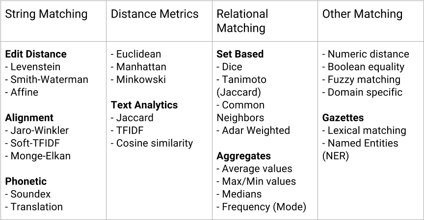
Figure 6-2. Spatializing similarity
Distance Metrics
When we think of how to measure the distance between two points, we usually think of a straight line, or Euclidean distance, represented in Figure 6-3 as the diagonal line. Manhattan distance, shown in Figure 6-3 as the three stepped paths, is similar, computed as the sum of the absolute differences of the Cartesian coordinates. Minkowski distance is a generalization of Euclidean and Manhattan distance, and defines the distance between two points in a normalized vector space.
However, as the vocabulary of our corpus grows, so does its dimensionality—and rarely in an evenly distributed way. For this reason, these distance measures are not always a very effective measure, since they assume all data is symmetric and that distance is the same in all dimensions.
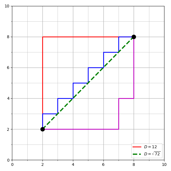
Figure 6-3. Euclidean versus Manhattan distance
By contrast, Mahalanobis distance, shown in Figure 6-4, is a multidimensional generalization of the measurement of how many standard deviations away a particular point is from a distribution of points. This has the effect of shifting and rescaling the coordinates with respect to the distribution. As such, Mahalanobis distance gives us a slightly more flexible way to define distances between documents; for instance, enabling us to identify similarities between utterances of different lengths.
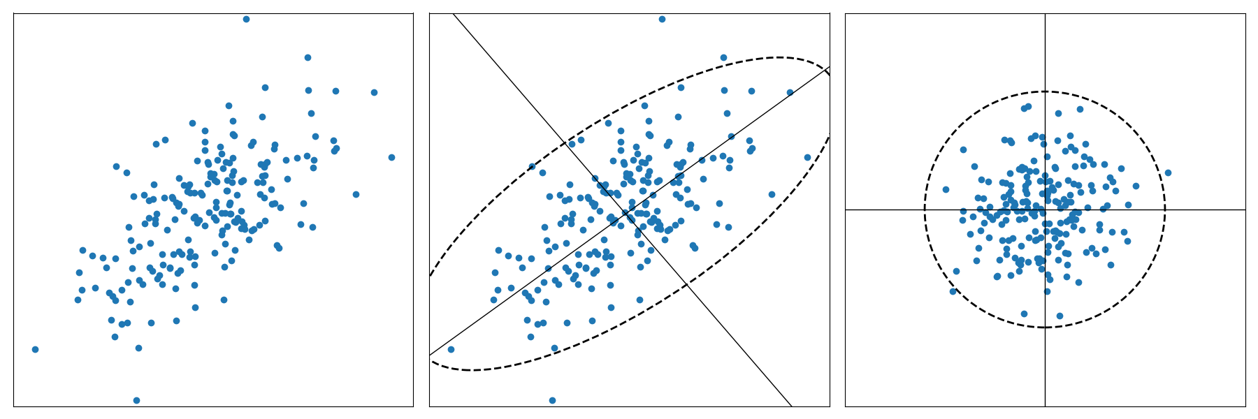
Figure 6-4. Mahalanobis distance
Jaccard distance defines similarity between finite sets as the quotient of their intersection and their union, as shown in Figure 6-5. For instance, we could measure the Jaccard distance between two documents A and B by dividing the number of unique words that appear in both A and B by the total number of unique words that appear in A and B. A value of 0 would indicate that the two documents have nothing in common, a 1 that they were the same document, and values between 0 and 1 indicating their relative degree of similarity.
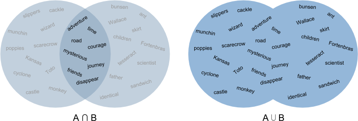
Figure 6-5. Jaccard distance
Edit distance measures the distance between two strings by the number of permutations needed to convert one into the other. There are multiple implementations of edit distance, all variations on Levenshtein distance, but with differing penalties for insertions, deletions, and substitutions, as well as potentially increased penalties for gaps and transpositions. In Figure 6-6 we can see that the edit distance between “woodman” and “woodland” includes penalties for one insertion and one substitution.
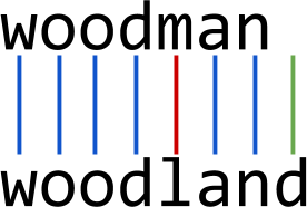
Figure 6-6. Edit distance
It is also possible to measure distances between vectors. For example, we can define two document vectors as similar by their TF–IDF distance; in other words, the magnitude to which they share the same unique terms relative to the rest of the words in the corpus. We can compute this using TF–IDF, as described in Chapter 4. We can also measure vector similarity with cosine distance, using the cosine of the angle between the two vectors to assess the degree to which they share the same orientation, as shown in Figure 6-7. In effect, the more parallel any two vectors are, the more similar the documents will be (regardless of their magnitude).
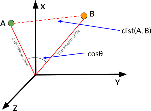
Figure 6-7. Cosine similarity
While Euclidean distance is often the default metric used in clustering model hyperparameters (as we’ll see in the next sections), we frequently find the most success using cosine distance.
Partitive Clustering
Now that we can quantify the similarity between any two documents, we can begin exploring unsupervised methods for finding similar groups of documents. Partitive clustering and agglomerative clustering are our two main approaches, and both separate documents into groups whose members share maximum similarity as defined by some distance metric. In this section, we will focus on partitive methods, which partition instances into groups that are represented by a central vector (the centroid) or described by a density of documents per cluster. Centroids represent an aggregated value (e.g., mean or median) of all member documents and are a convenient way to describe documents in that cluster.
As we saw in Chapter 5, the Baleen corpus is already categorized after a fashion, as each document is (human-)labeled with the categories of the RSS sources from which the data originated. However, some of these categories are not necessarily distinct (e.g., “tech” and “gaming”) and others are significantly more diffuse. For instance, the “news” corpus contains news on a range of topics, including political news, entertainment, science, and other current events. In this section, we will use clustering to establish subcategories within the “news” corpus, which might then be employed as target values for subsequent classification tasks.
k-means clustering
Because it has implementations in familiar libraries like NLTK and Scikit-Learn, k-means is a convenient place to start. A popular method for unsupervised learning tasks, the k-means clustering algorithm starts with an arbitrarily chosen number of clusters, k, and partitions the vectorized instances into clusters according to their proximity to the centroids, which are computed to minimize the within-cluster sum of squares.
We will begin by defining a class, KMeansClusters, which inherits from BaseEstimator and TransformerMixin so it will function inside a Scikit-Learn Pipeline. We’ll use NLTK’s implementation of k-means for our model, since it allows us to define our own distance metric. We initialize the NLTK KMeansClusterer with our desired number of clusters (k) and our preferred distance measure (cosine_distance), and avoid a result with clusters that contain no documents.
fromnltk.clusterimportKMeansClustererfromsklearn.baseimportBaseEstimator,TransformerMixinclassKMeansClusters(BaseEstimator,TransformerMixin):def__init__(self,k=7):"""k is the number of clustersmodel is the implementation of Kmeans"""self.k=kself.distance=nltk.cluster.util.cosine_distanceself.model=KMeansClusterer(self.k,self.distance,avoid_empty_clusters=True)
Now we’ll add our no-op fit() method and a transform() method that calls the internal KMeansClusterer model’s cluster() method, specifying that each document should be assigned a cluster. Our transform() method expects one-hot encoded documents, and by setting assign_clusters=True, it will return a list of the cluster assignments for each document:
deffit(self,documents,labels=None):returnselfdeftransform(self,documents):"""Fits the K-Means model to one-hot vectorized documents."""returnself.model.cluster(documents,assign_clusters=True)
To prepare our documents for our KMeansClusters class, we need to normalize and vectorize them first. For normalization, we’ll use a version of the TextNormalizer class we defined in “Creating a custom text normalization transformer”, with one small change to the tranform() method. Instead of returning a representation of documents as bags-of-words, this version of the TextNormalizer will perform stopwords removal and lemmatization and return a string for each document:
classTextNormalizer(BaseEstimator,TransformerMixin):...deftransform(self,documents):return[' '.join(self.normalize(doc))fordocindocuments]
To vectorize our documents after normalization and ahead of clustering, we’ll define a OneHotVectorizer class. For vectorization, we’ll use Scikit-Learn’s CountVectorizer with binary=True, which will wrap both frequency encoding and binarization. Our transform() method will return a representation of each document as a one-hot vectorized array:
fromsklearn.baseimportBaseEstimator,TransformerMixinfromsklearn.feature_extraction.textimportCountVectorizerclassOneHotVectorizer(BaseEstimator,TransformerMixin):def__init__(self):self.vectorizer=CountVectorizer(binary=True)deffit(self,documents,labels=None):returnselfdeftransform(self,documents):freqs=self.vectorizer.fit_transform(documents)return[freq.toarray()[0]forfreqinfreqs]
Now, we can create a Pipeline inside our main() execution to perform k-means clustering. We’ll initialize a PickledCorpusReader as defined in “Reading the Processed Corpus”, specifying that we want to use only the “news” category of our corpus. Then we’ll initialize a pipeline to streamline our custom TextNormalizer, OneHotVectorizer, and KMeansClusters classes. By calling fit_transform() on the pipeline, we perform each of these steps in sequence:
fromsklearn.pipelineimportPipelinecorpus=PickledCorpusReader('../corpus')docs=corpus.docs(categories=['news'])model=Pipeline([('norm',TextNormalizer()),('vect',OneHotVectorizer()),('clusters',KMeansClusters(k=7))])clusters=model.fit_transform(docs)pickles=list(corpus.fileids(categories=['news']))foridx,clusterinenumerate(clusters):("Document '{}' assigned to cluster {}.".format(pickles[idx],cluster))
Our result is a list of cluster assignments corresponding to each of the documents from our news category, which we can easily map back to the fileids of the pickled documents:
Document 'news/56d62554c1808113ffb87492.pickle' assigned to cluster 0.
Document 'news/56d6255dc1808113ffb874f0.pickle' assigned to cluster 5.
Document 'news/56d62570c1808113ffb87557.pickle' assigned to cluster 4.
Document 'news/56d625abc1808113ffb87625.pickle' assigned to cluster 2.
Document 'news/56d63a76c1808113ffb8841c.pickle' assigned to cluster 0.
Document 'news/56d63ae1c1808113ffb886b5.pickle' assigned to cluster 3.
Document 'news/56d63af0c1808113ffb88745.pickle' assigned to cluster 5.
Document 'news/56d64c7ac1808115036122b4.pickle' assigned to cluster 6.
Document 'news/56d64cf2c1808115036125f5.pickle' assigned to cluster 2.
Document 'news/56d65c2ec1808116aade2f8a.pickle' assigned to cluster 2.
...
We now have a preliminary model for clustering documents based on text similarity; now we should consider what we can do to optimize our results. However, unlike the case of classification, we don’t have a convenient measure to tell us if the “news” corpus has been correctly partitioned into subcategories—when it comes to unsupervised learning, we don’t have a ground truth. Instead, generally we would look to some human validation to see if our clusters make sense—are they meaningfully distinct? Are they sufficiently focused? In the next section, we’ll discuss what it might mean to “optimize” a clustering model.
Optimizing k-means
How can we “improve” a clustering model? In our case, this amounts to asking how we can make our results more interpretable and more useful. First, we can often make our results more interpretable by experimenting with different values of k. With k-means clustering, k-selection is often an iterative process; while there are rules of thumb, initial selection is often somewhat arbitrary.
Note
In “Silhouette Scores and Elbow Curves” we will discuss two visual techniques that can help guide experimentation with k-selection: silhouette scores and elbow curves.
We can also tune other parts of our pipeline; for example, instead of using one-hot encoding, we could switch to TF–IDF vectorization. Alternatively, in place of our TextNormalizer, we could introduce a feature selector that would select only a subset of the entire feature set (e.g., only the 5,000 most common tokens, excluding stopwords).
Note
Although the focus of this book is not big data, it is important to note that k-means does effectively scale for big data with the introduction of canopy clustering. Other text clustering algorithms, like LDA, are much more challenging to parallelize without additional tools (e.g., Tensorflow).
Keep in mind that k-means is not a lightweight algorithm and can be particularly slow with high-dimensional data such as text. If your clustering pipeline is very slow, you can optimize for speed by switching from the nltk.cluster module to using sklearn.cluster’s MiniBatchKMeans implementation. MiniBatchKMeans is a k-means variant that uses randomly sampled subsets (or “mini-batches”) of the entire training dataset to optimize the same objective function, but with a much-reduced computation time.
fromsklearn.clusterimportMiniBatchKMeansfromsklearn.baseimportBaseEstimator,TransformerMixinclassKMeansClusters(BaseEstimator,TransformerMixin):def__init__(self,k=7):self.k=kself.model=MiniBatchKMeans(self.k)deffit(self,documents,labels=None):returnselfdeftransform(self,documents):returnself.model.fit_predict(documents)
The trade-off is that our MiniBatchKMeans implementation, while faster, will use Euclidean distance, which is less effective for text. At the time of this writing, the Scikit-Learn implementations of KMeans and MiniBatchKMeans do not support the use of non-Euclidean distance measures.
Handling uneven geometries
The k-means algorithm makes several naive assumptions about data, presuming that it will be well-distributed, that clusters will have roughly comparable degrees of variance, and that they will be fundamentally spherical in nature. As such, there are many cases where k-means clustering will be unsuccessful; for instance, when outlier data points interfere with cluster coherence and when clusters have markedly different, or nonspherical densities. Using alternative distance measures, such as cosine or Mahalanobis distance, can help to address these cases.
Note
There are several other partitive techniques implemented in Scikit-Learn, such as affinity propagation, spectral clustering, and Gaussian mixtures, which may prove to be more performant in cases where k-means is not.
Ultimately, the advantages of using k-means make it an important tool in the natural language processing toolkit; k-means offers conceptual simplicity, producing tight, spherical clusters, convenient centroids that support model interpretability, and the guarantee of eventual convergence. In the rest of this chapter, we’ll explore some of the other, more sophisticated techniques we have found useful for text, but there’s no silver bullet, and a simple k-means approach is often a convenient place to start.
Hierarchical Clustering
In the previous section, we explored partitive methods, which divide points into clusters. By contrast, hierarchical clustering involves creating clusters that have a predetermined ordering from top to bottom. Hierarchical models can be either agglomerative, where clusters begin as single instances that iteratively aggregate by similarity until all belong to a single group, or divisive, where the data are gradually divided, beginning with all instances and finishing as single instances.
These methods create a dendrogram representation of the cluster structures, as shown in the lower left in Figure 6-8.
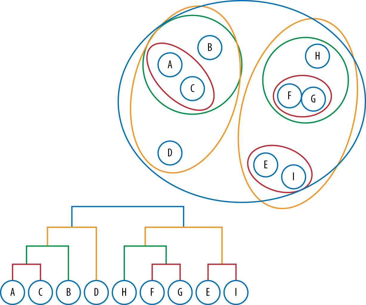
Figure 6-8. Hierarchical clustering
Agglomerative clustering
Agglomerative clustering iteratively combines the closest instances into clusters until all the instances belong to a single group. In the context of text data, the result is a hierarchy of variable-sized groups that describe document similarities at different levels or granularities.
We can switch our clustering implementation to an agglomerative approach fairly easily. We first define a HierarchicalClusters class, which initializes a Scikit-Learn AgglomerativeClustering model.
fromsklearn.clusterimportAgglomerativeClusteringclassHierarchicalClusters(object):def__init__(self):self.model=AgglomerativeClustering()
We add our no-op fit() method and a tranform() method, which calls the internal model’s fit_predict method, saving the resulting children and labels attributes for later use and returning the clusters.
...deffit(self,documents,labels=None):returnselfdeftransform(self,documents):"""Fits the agglomerative model to the given data."""clusters=self.model.fit_predict(documents)self.labels=self.model.labels_self.children=self.model.children_returnclusters
Next, we’ll put the pieces together into a Pipeline and inspect the cluster labels and membership of each of the children of each nonleaf node.
model=Pipeline([('norm',TextNormalizer()),('vect',OneHotVectorizer()),('clusters',HierarchicalClusters())])model.fit_transform(docs)labels=model.named_steps['clusters'].labelspickles=list(corpus.fileids(categories=['news']))foridx,fileidinenumerate(pickles):("Document '{}' assigned to cluster {}.".format(fileid,labels[idx]))
The results appear as follows:
Document 'news/56d62554c1808113ffb87492.pickle' assigned to cluster 1.
Document 'news/56d6255dc1808113ffb874f0.pickle' assigned to cluster 0.
Document 'news/56d62570c1808113ffb87557.pickle' assigned to cluster 1.
Document 'news/56d625abc1808113ffb87625.pickle' assigned to cluster 1.
Document 'news/56d63a76c1808113ffb8841c.pickle' assigned to cluster 1.
Document 'news/56d63ae1c1808113ffb886b5.pickle' assigned to cluster 0.
Document 'news/56d63af0c1808113ffb88745.pickle' assigned to cluster 1.
Document 'news/56d64c7ac1808115036122b4.pickle' assigned to cluster 1.
Document 'news/56d64cf2c1808115036125f5.pickle' assigned to cluster 0.
Document 'news/56d65c2ec1808116aade2f8a.pickle' assigned to cluster 0.
...
One of the challenges with agglomerative clustering is that we don’t have the benefit of centroids to use in labeling our document clusters as we did with the k-means example. Therefore, to enable us to visually explore the resultant clusters of our AgglomerativeClustering model, we will define a method plot_dendrogram to create a visual representation.
Our plot_dendrogram method will use the dendrogram method from SciPy and will also require Matplotlib’s pyplot. We use NumPy to compute a distance range between the child leaf nodes, and make an equal range of values to represent each child position. We then create a linkage matrix to hold the positions between each child and their distances. Finally we use SciPy’s dendrogram method, passing in the linkage matrix and any keyword arguments that can later be passed in to modify the figure.
importnumpyasnpfrommatplotlibimportpyplotaspltfromscipy.cluster.hierarchyimportdendrogramdefplot_dendrogram(children,**kwargs):# Distances between each pair of childrendistance=position=np.arange(children.shape[0])# Create linkage matrix and then plot the dendrogramlinkage_matrix=np.column_stack([children,distance,position]).astype(float)# Plot the corresponding dendrogramfig,ax=plt.subplots(figsize=(10,5))# set sizeax=dendrogram(linkage_matrix,**kwargs)plt.tick_params(axis='x',bottom='off',top='off',labelbottom='off')plt.tight_layout()plt.show()
children=model.named_steps['clusters'].childrenplot_dendrogram(children)
We can see the resulting plot in Figure 6-9. The first documents to be aggregated into the same cluster, those with the shortest branches, are the ones that exhibited the least variations. Those with the longest branches illustrate those with more variance, which were clustered later in the process.
Just as there are multiple ways of quantifying the difference between any two documents, there are also multiple criteria for establishing the linkages between them. Agglomerative clustering requires both a distance function and a linkage criterion. Scikit-Learn’s implementation defaults to the Ward criterion, which minimizes the within-cluster variance as each are successively merged. At each aggregation step, the algorithm finds the pair of clusters that contributes the least increase in total within-cluster variance after merging.
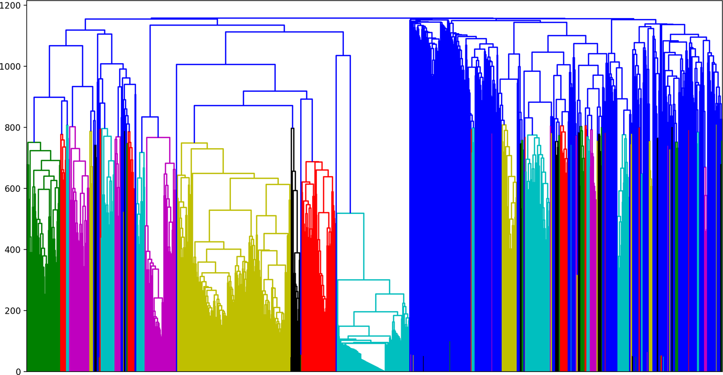
Figure 6-9. Dendrogram plot
Note
Other linkage criterion options in Scikit-Learn include "average", which uses the average of the distances between points in the clusters, and "complete", which uses the maximum distances between all points in the clusters.
As we can see from the results of our KMeansClusters and HierarchicalClusters, one of the challenges with both partitive and agglomerative clustering is that they don’t give much insight into why a document ended up in a particular cluster. In the next section, we’ll explore a different set of methods that expose strategies we can leverage not only to rapidly group our documents, but also to effectively describe their contents.
Modeling Document Topics
Now that we have organized our documents into piles, how should we go about labeling them and describing their contents? In this section, we’ll explore topic modeling, an unsupervised machine learning technique for abstracting topics from collections of documents. While clustering seeks to establish groups of documents within a corpus, topic modeling aims to abstract core themes from a set of utterances; clustering is deductive, while topic modeling is inductive.
Methods for topic modeling, and convenient open source implementations, have evolved significantly over the last decade. In the next section, we’ll compare three of these techniques: Latent Dirichlet Allocation (LDA), Latent Semantic Analysis (LSA), and Non-Negative Matrix Factorization (NNMF).
Latent Dirichlet Allocation
First introduced by David Blei, Andrew Ng, and Michael Jordan in 2003, Latent Dirichlet Allocation (LDA) is a topic discovery technique. It belongs to the generative probabilistic model family, in which topics are represented as the probability that each of a given set of terms will occur. Documents can in turn be represented in terms of a mixture of these topics. A unique feature of LDA models is that topics are not required to be distinct, and words may occur in multiple topics; this allows for a kind of topical fuzziness that is useful for handling the flexibility of language (Figure 6-10).
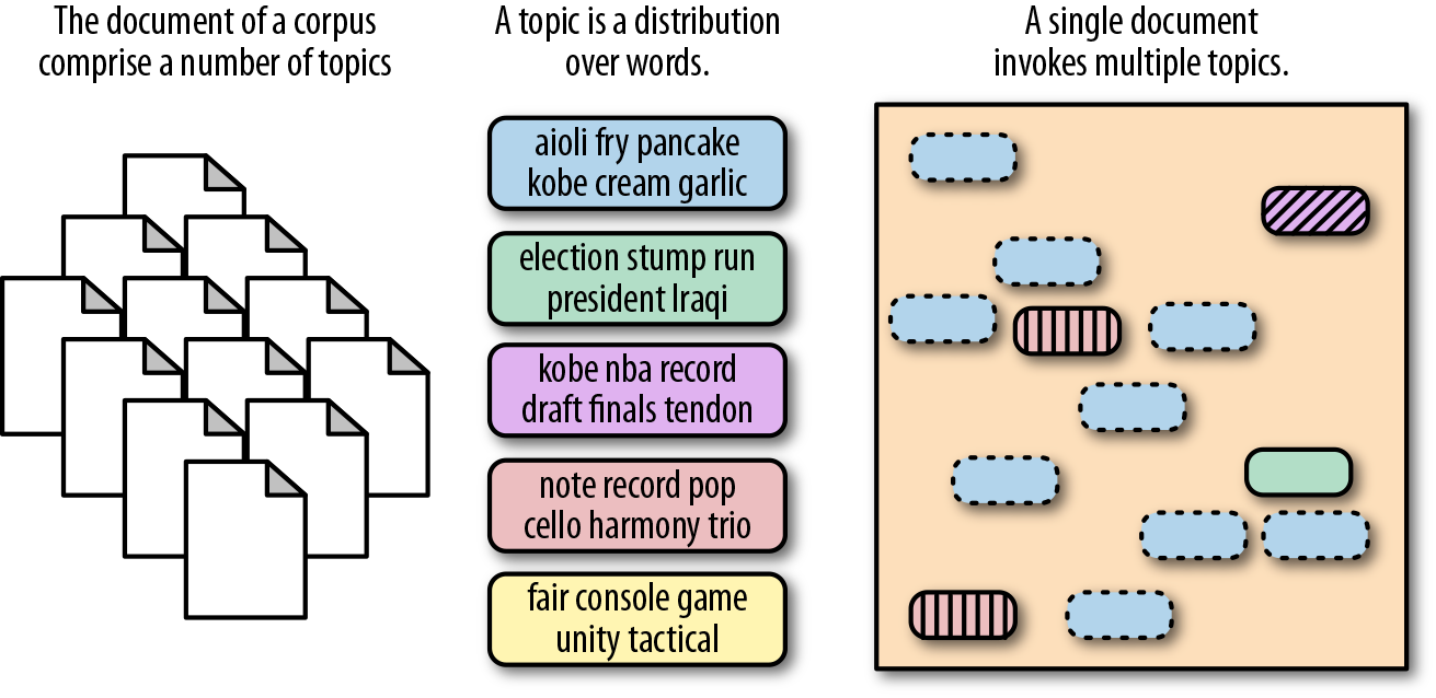
Figure 6-10. Latent Dirichlet Allocation
Blei et al. (2003) found that the Dirichlet prior, a continuous mixture distribution (a way of measuring a distribution over distributions), is a convenient way of discovering topics that occur across a corpus and also manifest in different mixtures within each document in the corpus.1 In effect, with a Latent Dirichlet Allocation, we are given an observed word or token, from which we attempt to model the probability of topics, the distribution of words for each topic, and the mixture of topics within a document.
To use topic models in an application, we need a tunable pipeline that will extrapolate topics from unstructured text data, and a method for storing the best model so it can be used on new, incoming data. We’ll do this first with Scikit-Learn and then with Gensim.
In Scikit-Learn
We begin by creating a class, SklearnTopicModels. The __init__ function instantiates a pipeline with our TextNormalizer, CountVectorizer, and Scikit-Learn’s implementation of LatentDirichletAllocation. We must specify a number of topics (here 50), just as we did with k-means clustering.
fromsklearn.pipelineimportPipelinefromsklearn.decompositionimportLatentDirichletAllocationfromsklearn.feature_extraction.textimportCountVectorizerclassSklearnTopicModels(object):def__init__(self,n_topics=50):"""n_topics is the desired number of topics"""self.n_topics=n_topicsself.model=Pipeline([('norm',TextNormalizer()),('vect',CountVectorizer(tokenizer=identity,preprocessor=None,lowercase=False)),('model',LatentDirichletAllocation(n_topics=self.n_topics)),])
Note
In the rest of the examples in the chapter, we will want to use the original version of TextNormalizer from “Creating a custom text normalization transformer”, which returns a representation of documents as bags-of-words.
We then create a fit_transform method, which will call the internal fit and transform methods of each step of our pipeline:
deffit_transform(self,documents):self.model.fit_transform(documents)returnself.model
Now that we have a way to create and fit the pipeline, we want some mechanism to inspect our topics. The topics aren’t labeled, and we don’t have a centroid with which to produce a label as we would with centroidal clustering. Instead, we will inspect each topic in terms of the words it has the highest probability of generating.
We create a get_topics method, which steps through our pipeline object to retrieve the fitted vectorizer and extracts the tokens from its get_feature_names() attribute. We loop through the components_ attribute of the LDA model, and for each of the topics and its corresponding index, we reverse-sort the numbered tokens by weight such that the 25 highest weighted terms are ranked first. We then retrieve the corresponding tokens from the feature names and store our topics as a dictionary where the key is the index of one of the 50 topics and the values are the top words associated with that topic.
defget_topics(self,n=25):"""n is the number of top terms to show for each topic"""vectorizer=self.model.named_steps['vect']model=self.model.steps[-1][1]names=vectorizer.get_feature_names()topics=dict()foridx,topicinenumerate(model.components_):features=topic.argsort()[:-(n-1):-1]tokens=[names[i]foriinfeatures]topics[idx]=tokensreturntopics
We can now instantiate a SklearnTopicModels object, and fit and transform the pipeline on our corpus documents. We assign the result of the get_topics() attribute (a Python dictionary) to a topics variable and unpack the dictionary, printing out the corresponding topics and their most informative terms:
if__name__=='__main__':corpus=PickledCorpusReader('corpus/')lda=SklearnTopicModels()documents=corpus.docs()lda.fit_transform(documents)topics=lda.get_topics()fortopic,termsintopics.items():("Topic #{}:".format(topic+1))(terms)
The results appear as follows:
Topic #1:
['science', 'scientist', 'data', 'daviau', 'human', 'earth', 'bayesian',
'method', 'scientific', 'jableh', 'probability', 'inference', 'crater',
'transhumanism', 'sequence', 'python', 'engineer', 'conscience',
'attitude', 'layer', 'pee', 'probabilistic', 'radio']
Topic #2:
['franchise', 'rhoden', 'rosemary', 'allergy', 'dewine', 'microwave',
'charleston', 'q', 'pike', 'relmicro', '($', 'wicket', 'infant',
't20', 'piketon', 'points', 'mug', 'snakeskin', 'skinnytaste',
'frankie', 'uninitiated', 'spirit', 'kosher']
Topic #3:
['cosby', 'vehicle', 'moon', 'tesla', 'module', 'mission', 'hastert',
'air', 'mars', 'spacex', 'kazakhstan', 'accuser', 'earth', 'makemake',
'dragon', 'model', 'input', 'musk', 'recall', 'buffon', 'stage',
'journey', 'capsule']
...
The Gensim way
Gensim also exposes an implementation for Latent Dirichlet Allocation, which offers some convenient attributes over Scikit-Learn. Conveniently, Gensim (starting with version 2.2.0) provides a wrapper for its LDAModel, called ldamodel.LdaTransformer, which makes integration with a Scikit-Learn pipeline that much more convenient.
To use Gensim’s LdaTransformer, we need to create a custom Scikit-Learn wrapper for Gensim’s TfidfVectorizer so that it can function inside a Scikit-Learn Pipeline. GensimTfidfVectorizer will vectorize our documents ahead of LDA, as well as saving, holding, and loading a custom-fitted lexicon and vectorizer for later use.
classGensimTfidfVectorizer(BaseEstimator,TransformerMixin):def__init__(self,dirpath=".",tofull=False):"""Pass in a directory that holds the lexicon in corpus.dict and theTF-IDF model in tfidf.model.Set tofull = True if the next thing is a Scikit-Learn estimatorotherwise keep False if the next thing is a Gensim model."""self._lexicon_path=os.path.join(dirpath,"corpus.dict")self._tfidf_path=os.path.join(dirpath,"tfidf.model")self.lexicon=Noneself.tfidf=Noneself.tofull=tofullself.load()defload(self):ifos.path.exists(self._lexicon_path):self.lexicon=Dictionary.load(self._lexicon_path)ifos.path.exists(self._tfidf_path):self.tfidf=TfidfModel().load(self._tfidf_path)defsave(self):self.lexicon.save(self._lexicon_path)self.tfidf.save(self._tfidf_path)
If the model has already been fit, we can initialize the GensimTfidfVectorizer with a lexicon and vectorizer that can be loaded from disk using the load method. We also implement a save() method, which we will call after fitting the vectorizer.
Next, we implement fit() by creating a Gensim Dictionary object, which takes as an argument a list of normalized documents. We instantiate a Gensim TfidfModel, passing in as an argument the list of documents, each of which have been passed through lexicon.doc2bow, and been transformed into bags of words. We then call the save method, which serializes our lexicon and vectorizer and saves them to disk. Finally, the fit() method returns self to conform with the Scikit-Learn API.
deffit(self,documents,labels=None):self.lexicon=Dictionary(documents)self.tfidf=TfidfModel([self.lexicon.doc2bow(doc)fordocindocuments],id2word=self.lexicon)self.save()returnself
We then implement our transform() method, which creates a generator that loops through each of our normalized documents and vectorizes them using the fitted model and their bag-of-words representation. Because the next step in our pipeline will be a Gensim model, we initialized our vectorizer to set tofull=False, so that it would output a sparse document format (a sequence of 2-tuples). However, if we were going to use a Scikit-Learn estimator next, we would want to initialize our GensimTfidfVectorizer with tofull=True, which here in our transform method would convert the sparse format into the needed dense representation for Scikit-Learn, an np array.
deftransform(self,documents):defgenerator():fordocumentindocuments:vec=self.tfidf[self.lexicon.doc2bow(document)]ifself.tofull:yieldsparse2full(vec)else:yieldvecreturnlist(generator())
We now have a custom wrapper for our Gensim vectorizer, and here in GensimTopicModels, we put all of the pieces together:
fromsklearn.pipelineimportPipelinefromgensim.sklearn_apiimportldamodelclassGensimTopicModels(object):def__init__(self,n_topics=50):"""n_topics is the desired number of topics"""self.n_topics=n_topicsself.model=Pipeline([('norm',TextNormalizer()),('vect',GensimTfidfVectorizer()),('model',ldamodel.LdaTransformer(num_topics=self.n_topics))])deffit(self,documents):self.model.fit(documents)returnself.model
We can now fit our pipeline with our corpus.docs:
if__name__=='__main__':corpus=PickledCorpusReader('../corpus')gensim_lda=GensimTopicModels()docs=[list(corpus.docs(fileids=fileid))[0]forfileidincorpus.fileids()]gensim_lda.fit(docs)
In order to inspect the topics, we can retrieve them from the LDA step, which is the gensim_model attribute from the last step of our pipeline. We can then use the Gensim LDAModel show_topics method to view the topics and the token-weights for the top ten most influential tokens:
lda=gensim_lda.model.named_steps['model'].gensim_model(lda.show_topics())
We can also define a function get_topics, which given the fitted LDAModel and vectorized corpus, will retrieve the highest-weighted topic for each of the documents in the corpus:
defget_topics(vectorized_corpus,model):fromoperatorimportitemgettertopics=[max(model[doc],key=itemgetter(1))[0]fordocinvectorized_corpus]returntopicslda=gensim_lda.model.named_steps['model'].gensim_modelcorpus=[gensim_lda.model.named_steps['vect'].lexicon.doc2bow(doc)fordocingensim_lda.model.named_steps['norm'].transform(docs)]topics=get_topics(corpus,lda)fortopic,docinzip(topics,docs):("Topic:{}".format(topic))(doc)
Visualizing topics
Oftentimes with unsupervised learning techniques, it is helpful to be able to visually explore the results of a model, since traditional model evaluation techniques are useful only for supervised learning problems. Visualization techniques for text analytics will be discussed in greater detail in Chapter 8, but here we will briefly explore the use of the pyLDAvis library, which is designed to provide a visual interface for interpreting the topics derived from a topic model.
PyLDAvis works by extracting information from fitted LDA topic models to inform an interactive web-based visualization, which can easily be run from inside a Jupyter notebook or saved as HTML. In order visualize our document topics with pyLDAvis, we can fit our pipeline inside a Jupyter notebook as follows:
importpyLDAvisimportpyLDAvis.gensimlda=gensim_lda.model.named_steps['model'].gensim_modelcorpus=[gensim_lda.model.named_steps['vect'].lexicon.doc2bow(doc)fordocingensim_lda.model.named_steps['norm'].transform(docs)]lexicon=gensim_lda.model.named_steps['vect'].lexicondata=pyLDAvis.gensim.prepare(model,corpus,lexicon)pyLDAvis.display(data)
The key method pyLDAvis.gensim.prepare takes as an argument the LDA model, the vectorized corpus, and the derived lexicon and produces, upon calling display, visualizations like the one shown in Figure 6-11.
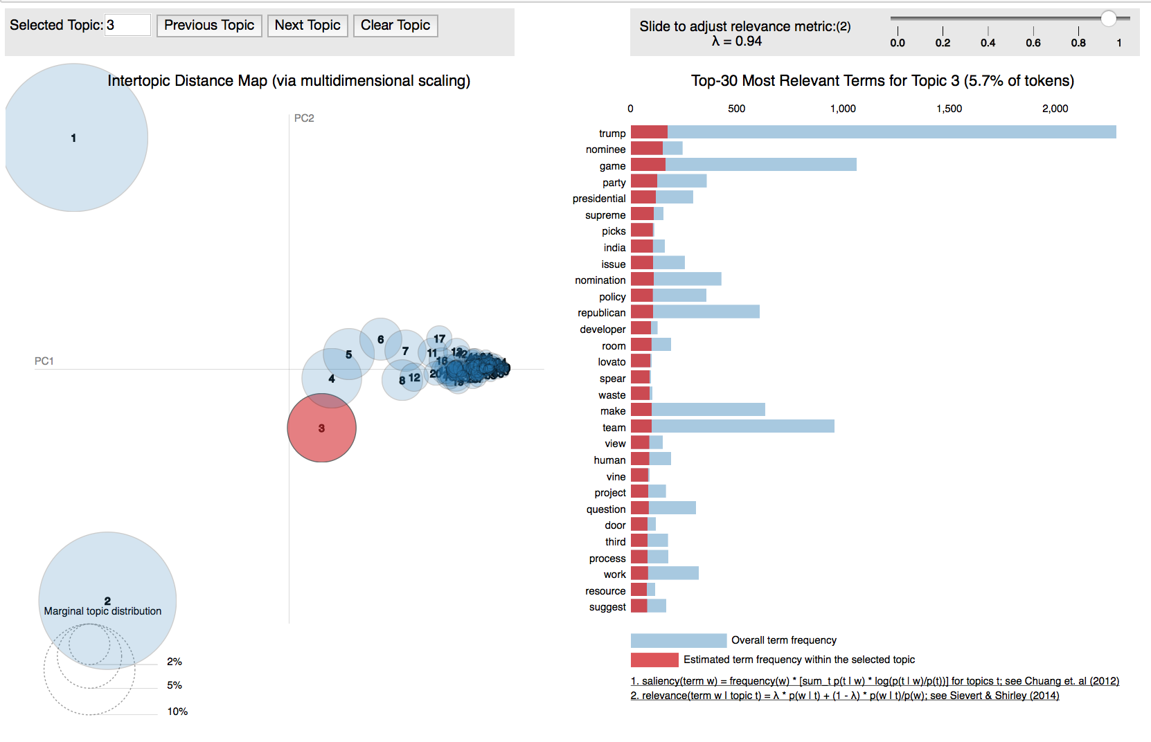
Figure 6-11. Interactive topic model visualization with pyLDAvis
Latent Semantic Analysis
Latent Semantic Analysis (LSA) is a vector-based approach first suggested as a topic modeling technique by Deerwester et al in 1990.2
While Latent Dirichlet Allocation works by abstracting topics from documents, which can then be used to score documents by their proportion of topical terms, Latent Semantic Analysis simply finds groups of documents with the same words. The LSA approach to topic modeling (also known as Latent Semantic Indexing) identifies themes within a corpus by creating a sparse term-document matrix, where each row is a token and each column is a document. Each value in the matrix corresponds to the frequency with which the given term appears in that document, and can be normalized using TF–IDF. Singular Value Decomposition (SVD) can then be applied to the matrix to factorize into matrices that represent the term-topics, the topic importances, and the topic-documents.
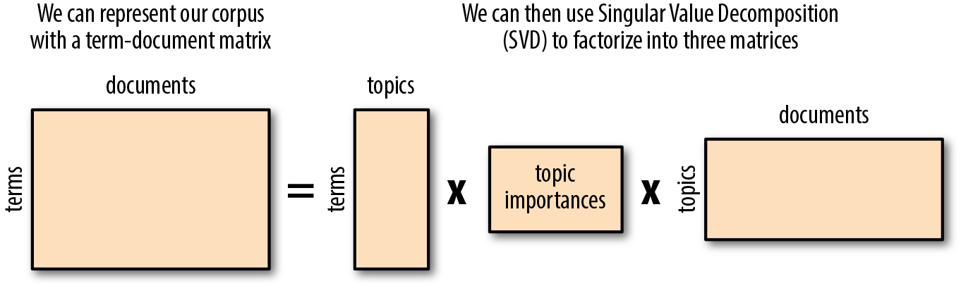
Figure 6-12. Latent Semantic Analysis
Using the derived diagonal topic importance matrix, we can identify the topics that are the most significant in our corpus, and remove rows that correspond to less important topic terms. Of the remaining rows (terms) and columns (documents), we can assign topics based on their highest corresponding topic importance weights.
In Scikit-Learn
To do Latent Semantic Analysis with Scikit-Learn, we will make a pipeline that normalizes our text, creates a term-document matrix using a CountVectorizer, and then employs TruncatedSVD, which is the Scikit-Learn implementation of Singular Value Decomposition. Scikit-Learn’s implementation only computes the k largest singular values, where k is a hyperparameter that we must specify via the n_components attribute. Fortunately, this requires very little refactoring of the __init__ method we created for our SklearnTopicModels class!
classSklearnTopicModels(object):def__init__(self,n_topics=50,estimator='LDA'):"""n_topics is the desired number of topicsTo use Latent Semantic Analysis, set estimator to 'LSA',otherwise, defaults to Latent Dirichlet Allocation ('LDA')."""self.n_topics=n_topicsifestimator=='LSA':self.estimator=TruncatedSVD(n_components=self.n_topics)else:self.estimator=LatentDirichletAllocation(n_topics=self.n_topics)self.model=Pipeline([('norm',TextNormalizer()),('tfidf',CountVectorizer(tokenizer=identity,preprocessor=None,lowercase=False)),('model',self.estimator)])
Our original fit_transform and get_topics methods that we defined for our Scikit-Learn implementation of the Latent Dirichlet Allocation pipeline will not require any modification to work with our newly refactored SklearnTopicModels class, so we can easily switch between the two algorithms to see which performs best according to our application and document context.
The Gensim way
Updating our GensimTopicModels class to enable a Latent Semantic Analysis pipeline is much the same. We again use our TextNormalizer, followed by the GensimTfidfVectorizer we used in our Latent Dirichlet Allocation pipeline, and finally the Gensim LsiModel wrapper exposed through the gensim.sklearn_api module, lsimodel.LsiTransformer:
fromgensim.sklearn_apiimportlsimodel,ldamodelclassGensimTopicModels(object):def__init__(self,n_topics=50,estimator='LDA'):"""n_topics is the desired number of topicsTo use Latent Semantic Analysis, set estimator to 'LSA'otherwise defaults to Latent Dirichlet Allocation."""self.n_topics=n_topicsifestimator=='LSA':self.estimator=lsimodel.LsiTransformer(num_topics=self.n_topics)else:self.estimator=ldamodel.LdaTransformer(num_topics=self.n_topics)self.model=Pipeline([('norm',TextNormalizer()),('vect',GensimTfidfVectorizer()),('model',self.estimator)])
We can now switch between the two Gensim algorithms with the estimator keyword argument.
Non-Negative Matrix Factorization
Another unsupervised technique that can be used for topic modeling is non-negative matrix factorization (NNMF). First introduced by Pentti Paatero and Unto Tapper (1994)3 and popularized in a Nature article by Daniel Lee and H. Sebastian Seung (1999),4 NNMF has many applications, including spectral data analysis, collaborative filtering for recommender systems, and topic extraction (Figure 6-13).
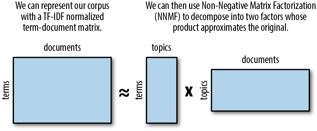
Figure 6-13. Non-negative matrix factorization
To apply NNMF for topic modeling, we begin by representing our corpus as we did with our Latent Semantic Analysis, as a TF–IDF normalized term-document matrix. We then decompose the matrix into two factors whose product approximates the original, such that every value in both factors is either positive or zero. The resulting matrices illustrate topics positively related to terms and documents of the corpus.
In Scikit-Learn
Scikit-Learn’s implementation of non-negative matrix factorization is the sklearn.decomposition.NMF class. With a minor amount of refactoring to the __init__ method of our SklearnTopicModels class, we can easily implement NNMF in our pipeline without any additional changes needed:
fromsklearn.decompositionimportNMFclassSklearnTopicModels(object):def__init__(self,n_topics=50,estimator='LDA'):"""n_topics is the desired number of topicsTo use Latent Semantic Analysis, set estimator to 'LSA',To use Non-Negative Matrix Factorization, set estimator to 'NMF',otherwise, defaults to Latent Dirichlet Allocation ('LDA')."""self.n_topics=n_topicsifestimator=='LSA':self.estimator=TruncatedSVD(n_components=self.n_topics)elifestimator=='NMF':self.estimator=NMF(n_components=self.n_topics)else:self.estimator=LatentDirichletAllocation(n_topics=self.n_topics)self.model=Pipeline([('norm',TextNormalizer()),('tfidf',CountVectorizer(tokenizer=identity,preprocessor=None,lowercase=False)),('model',self.estimator)])
So which topic modeling algorithm is best? Anecdotally,5 LSA is sometimes considered better for learning descriptive topics, which is helpful with longer documents and more diffuse corpora. Latent Dirichlet Allocation and non-negative matrix factorization, on the other hand, can be better for learning compact topics, which is useful for creating succinct labels from topics.
Ultimately, the best model will depend a great deal on the corpus you are working with and the goals of your application. Now you are equipped with the tools to experiment with multiple models to determine which works best for your use case!
Conclusion
In this chapter, we’ve seen that unsupervised machine learning can be tricky since there is no surefire way to evaluate the performance of a model. Nonetheless, distance-based techniques that allow us to quantify the similarities between documents can be an effective and fast method of dealing with large corpora to present interesting and relevant information.
As we discussed, k-means is an effective general-purpose clustering technique that scales well to large corpora (particularly if using the NLTK implementation with cosine distance, or the Scikit-Learn MiniBatchKMeans), especially if there aren’t too many clusters and the geometry isn’t too complex. Agglomerative clustering is a useful alternative in cases where there are a large number of clusters and data is less evenly distributed.
We also learned that effectively summarizing a corpus of unlabeled documents often requires not only a priori categorization, but also a method for describing those categories. This makes topic modeling—whether with Latent Dirichlet Allocation, Latent Semantic Analysis, or non-negative matrix factorization—another essential tool for the applied text analytics toolkit.
Clusters can be an excellent starting point to begin annotating a dataset for supervised methods that can be evaluated upon. Creating collections of similar documents can lead to more complex structures like graph relationships (which we’ll see more of in Chapter 9) that lead to more impactful downstream analysis. In Chapter 7, we’ll take a closer look at some more advanced contextual feature engineering strategies that will allow us to capture some of those complex structures for more effective text modeling.
1 David M. Blei, Andrew Y. Ng, and Michael I. Jordan, Latent Dirichlet Allocation, (2003) https://stanford.io/2GJBHR1
2 Scott Deerwester, Susan T. Dumais, George W. Furnas, Thomas K. Landauer, and Richard Harshman, Indexing by Latent Semantic Analysis, (1990) http://bit.ly/2JHWx57
3 Pentti Paatero and Unto Tapper, Positive matrix factorization: A non‐negative factor model with optimal utilization of error estimates of data values, (1994) http://bit.ly/2GOFdJU
4 Daniel D. Lee and H. Sebastian Seung, Learning the parts of objects by non-negative matrix factorization, (1999) http://bit.ly/2GJBIV5
5 Keith Stevens, Philip Kegelmeyer, David Andrzejewski, and David Buttler, Exploring Topic Coherence over many models and many topics, (2012) http://bit.ly/2GNHg11