Identifying Classification Problems

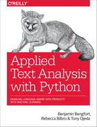
It may not necessarily be immediately obvious how to compose application problems into classification solutions, but it helps to understand that most language-aware data products are actually composed of multiple models and submodels. For example, a recommendation system such as the one shown in Figure 5-1 may have classifiers that identify a product’s target age (e.g., a youth versus an adult bicycle), gender (women’s versus men’s clothing), or category (e.g., electronics versus movies) by classifying the product’s description or other attributes. Product reviews may then be classified to detect quality or to determine similar products. These classes then may be used as features in downstream models or may be used to create partitions for ensemble models.

The combination of multiple classifiers has been incredibly powerful, particularly in recent years, and for several types of text classification applications. From email clients that incorporate spam filtering to applications that can predict political bias of news articles, the uses for classification are almost as numerous as the number of categories that we assign to things—and humans are excellent taxonomists. Newer applications combine text and image learning to enhance newer forms of media—from automatic captioning to scene recognition, all of which leverage classification techniques.

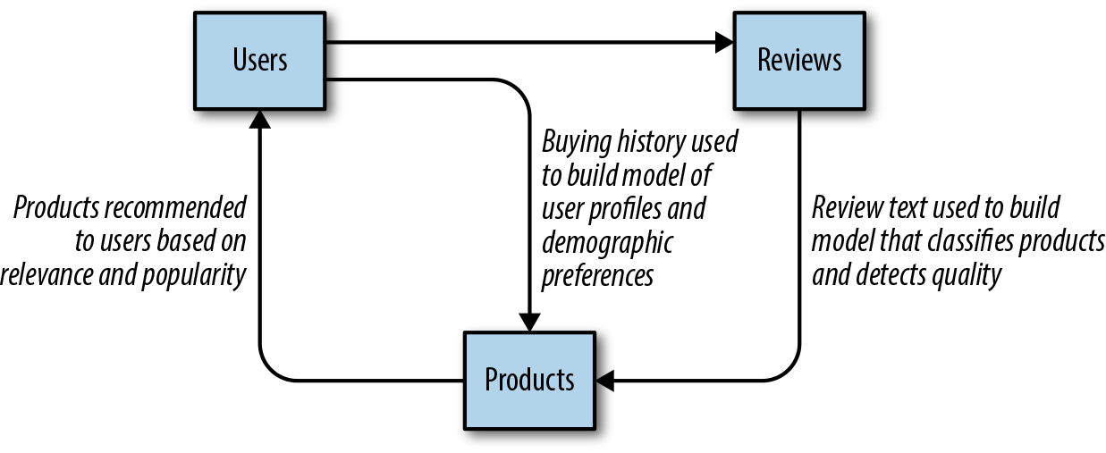
Figure 5-1. Multimodel product recommendation engine

The spam classification example has recently been displaced by a new vogue: sentiment analysis. Sentiment analysis models attempt to predict positive (“I love writing Python code”) or negative (“I hate it when people repeat themselves”) sentiment based on content and has gained significant popularity thanks to the expressiveness of social media. Because companies are involved in a more general dialogue where they do not control the information channel (such as reviews of their products and services), there is a belief that sentiment analysis can assist with targeted customer support or even model corporate performance. However, as we saw briefly in Chapter 1 and which we’ll explore more fully in Chapter 12, the complexities and nuances inherent in language context make sentiment analysis less straightforward than spam detection.

If sentiment can be explored through textual content, what about other external labels, political bias, for example? Recent work has used expressions in the American presidential campaign to create models that can detect partisan polarity (or its absence). An interesting result from these efforts is that the use of per-user models (trained on specific users’ data) provides more effective context than a global, generalizable model (trained on data pooled from many users).¹ Another real-world application is the automatic topic classification of text: by using blogs that publish content in a single domain (e.g., a cooking blog doesn’t generally discuss cinema), it is possible to create classifiers that can detect topics in uncategorized sources such as news articles.

So what do all these examples have in common? First, a unique external target defined by the application: e.g., what do we want to measure? Whether we want to filter spam, detect sentiment or political polarity, a specific topic, or language being spoken, the application defines the classes. The second commonality is the observation that by reading the content of the document or utterance, it is possible to make a judgment about the class. With these two rules of thumb, it becomes possible to employ automatic classification in a variety of places: troll detection, reading level, product category, entertainment rating, name detection, author identification, and more.

Classifier Models

The nice thing about the Naive Bayesian method used in the classic spam identification problem is that both the construction of the model (requiring only a single pass through the corpus) and predictions (computation of a probability via the product of an input vector with the underlying truth table) are extremely fast. The performance of Naive Bayes meant a machine learning model that could keep up with email-sized applications. Accuracy could be further improved by adding nontext features like the IP or email address of the sender, the number of included images, the use of numbers in spelling "v14gr4", etc.

Naive Bayes is an online model, meaning that it can be updated in real time without retraining from scratch (simply update the underlying truth table and token probabilities). This meant that email service providers could keep up with spammer reactions by simply allowing the user to mark offending emails as spam—updating the underlying model for everyone.

There are a wide variety of classification models and mechanisms that are comparatively more mathematically diverse than the linear models primarily used for regression. From instance-based methods that use distance-based similarity, partitive schemes, and Bayesian probability, to linear and nonlinear approximation and neural modeling, text analysis applications have many choices for model families. However, all classifier model families have the same basic workflow, and with Scikit-Learn Estimator objects, they can be employed in a procedural fashion and compared using cross-validation to select the best performing predictor.

The classification workflow occurs in two phases: a build phase and an operational phase as shown in Figure 5-2. In the build phase, a corpus of documents is transformed into feature vectors. The document features, along with their annotated labels (the category or class we want the model to learn), are then passed into a classification algorithm that defines its internal state along with the learned patterns. Once trained or fitted, a new document can be vectorized into the same space as the training data and passed to the predictive algorithm, which returns the assigned class label for the document.

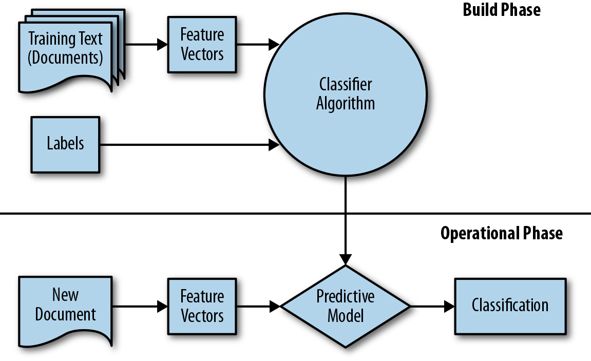
Figure 5-2. Classification workflow

Binary classifiers have two classes whose relationship is important: only the two classes are possible and one class is the opposite of the other (e.g., on/off, yes/no, etc.). In probabilistic terms, a binary classifier with classes A and B assumes that P(B) = 1 - P(A). However, this is frequently not the case. Consider sentiment analysis; if a document is not positive, is it necessarily negative? If some documents are neutral (which is often the case), adding a third class to our classifier may significantly increase its ability to identify the positive and negative documents. This then becomes a multiclass problem with multiple binary classes—for example, A and ¬A (not A) and B and ¬B (not B).

Cross-Validation

One of the biggest challenges of applied machine learning is defining a stopping criterion upfront—how do we know when our model is good enough to deploy? When is it time to stop tuning? Which model is the best for our use case? Cross-validation is an essential tool for scoping these kinds of applications, since it will allow us to compare models using training and test splits and estimate in advance which model will be most performant for our use case.

Our primary goal is to fit a classifier that succeeds in detecting separability in the training data and is also generalizable to unseen data. Separability means that our feature space has been correctly defined such that a meaningful decision space can be constructed to delineate classes. Generalizability means that the model is mostly accurate on making predictions on unseen data that was not part of the training dataset.

The trick is to walk the line between underfitting and overfitting. An underfit model has low variance, generally making the same predictions every time, but with extremely high bias, because the model deviates from the correct answer by a significant amount. Underfitting is symptomatic of not having enough data points, or not training a complex enough model. An overfit model, on the other hand, has memorized the training data and is completely accurate on data it has seen before, but varies widely on unseen data. Neither an overfit nor underfit model is generalizable—that is, able to make meaningful predictions on unseen data.

There is a trade-off between bias and variance, as shown in Figure 5-3. Complexity increases with the number of features, parameters, depth, training epochs, etc. As complexity increases and the model overfits, the error on the training data decreases, but the error on test data increases, meaning that the model is less generalizable.

Figure 5-3. Bias–variance trade-off

The goal is therefore to find the optimal point with enough model complexity so as to avoid underfit (decreasing the bias) without injecting error due to variance. To find that optimal point, we need to evaluate our model on data that it was not trained on. The solution is cross-validation: a multiround experimental method that partitions the data such that part of the data is reserved for testing and not fit upon to reduce error due to overfit.

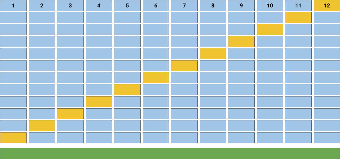
Figure 5-4. k-fold cross-validation

Cross-validation starts by shuffling the data (to prevent any unintentional ordering errors) and splitting it into k folds as shown in Figure 5-4. Then k models are fit on $\frac{k-1}{k}$ of the data (called the training split) and evaluated on $\frac{1}{k}$ of the data (called the test split). The results from each evaluation are averaged together for a final score, then the final model is fit on the entire dataset for operationalization.

from sklearn.model_selection import KFold

class CorpusLoader(object):

    def __init__(self, reader, folds=12, shuffle=True, categories=None):
        self.reader = reader
        self.folds  = KFold(n_splits=folds, shuffle=shuffle)
        self.files  = np.asarray(self.reader.fileids(categories=categories))

    def fileids(self, idx=None):
        if idx is None:
            return self.files
        return self.files[idx]

    def documents(self, idx=None):
        for fileid in self.fileids(idx):
            yield list(self.reader.docs(fileids=[fileid]))

    def labels(self, idx=None):
        return [
            self.reader.categories(fileids=[fileid])[0]
            for fileid in self.fileids(idx)
        ]

    def __iter__(self):
        for train_index, test_index in self.folds.split(self.files):
            X_train = self.documents(train_index)
            y_train = self.labels(train_index)

            X_test = self.documents(test_index)
            y_test = self.labels(test_index)

            yield X_train, X_test, y_train, y_test

Model Construction

As we learned in Chapter 4, Scikit-Learn Pipelines provide a mechanism for coordinating the vectorization process with the modeling process. We can start with a pipeline that normalizes our text, vectorizes it, and then passes it directly into a classifier. This will allow us to compare different text classification models such as Naive Bayes, Logistic Regression, and Support Vector Machines. Finally, we can apply a feature reduction technique such as Singular Value Decomposition to see if that improves our modeling.

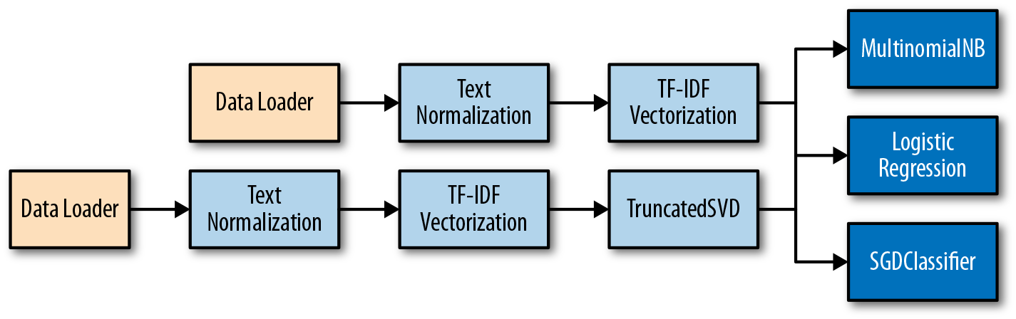
Figure 5-5. Simple classification pipelines

The end result is that we’ll be constructing six classification models: one for each of the three models and for the two pipeline combinations as shown in Figure 5-5. We will go ahead and use the default hyperparameters for each of these models initially so that we can start getting results.

We’ll add a create_pipeline function that takes an instantiated estimator as its first argument and a boolean indicating whether or not to apply decomposition to reduce the number of features. Our pipeline takes advantage of the TextNormalizer we built in Chapter 4 that uses WordNet lemmatization to reduce the number of overall word classes. Because we’ve already preprocessed and normalized the text, we must pass an identity function as the TfidfVectorizer tokenizer function; an identity function is simply a function that returns its arguments. Moreover, we can prevent preprocessing and lowercase by setting the appropriate arguments when instantiating the vectorizer.

from sklearn.pipeline import Pipeline
from sklearn.decomposition import TruncatedSVD
from sklearn.feature_extraction.text import TfidfVectorizer

def identity(words):
    return words

def create_pipeline(estimator, reduction=False):

    steps = [
        ('normalize', TextNormalizer()),
        ('vectorize', TfidfVectorizer(
            tokenizer=identity, preprocessor=None, lowercase=False
        ))
    ]

    if reduction:
        steps.append((
            'reduction', TruncatedSVD(n_components=10000)
        ))

    # Add the estimator
    steps.append(('classifier', estimator))
    return Pipeline(steps)

We can now quickly generate our models as follows:

from sklearn.linear_model import LogisticRegression
from sklearn.naive_bayes import MultinomialNB
from sklearn.linear_model import SGDClassifier

models = []
for form in (LogisticRegression, MultinomialNB, SGDClassifier):
    models.append(create_pipeline(form(), True))
    models.append(create_pipeline(form(), False))

The models list now contains six model forms—instantiated pipelines that include specific vectorization and feature extraction methods (feature analysis), a specific algorithm, and specific hyperparameters (currently set to the Scikit-Learn defaults).

Fitting the models given a training dataset of documents and their associated labels can be done as follows:

for model in models:
    model.fit(train_docs, train_labels)

By calling the fit() method on each model, the documents and labels from the training dataset are sent into the beginning of each pipeline. The transformers have their fit() methods called, then the data is passed into their transform() method. The transformed data is then passed to the fit() of the next transformer for each step in the sequence. The final estimator, in this case one of our classification algorithms, will have its fit() method called on the completely transformed data. Calling fit() will transform the input of preprocessed documents (lists of paragraphs that are lists of sentences, that are lists of tokens, tag tuples) into a two-dimensional numeric array, to which we can then apply optimization algorithms.

Model Evaluation

So which model was best? As with vectorization, model selection is data-, use case-, and application-specific. In our case, we want to know which model combination will be best at predicting the hobby category of a document based on its text. Because we have the correct target values from our test dataset, we can compare the predicted answers to the correct ones and determine the percent of the time the model is correct, effectively scoring each model with respect to its global accuracy.

Let’s compare our models. We’ll use the CorpusLoader we created in “Streaming access to k splits” to get our train_test_splits for our cross-validation folds. Then, for each fold, we will fit the model on the training data and the accompanying labels, then create a prediction vector off the test data. Next, we will pass the actual and the predicted labels for each fold to a score function and append the score to a list. Finally, we will average the results across all folds to get a single score for the model.

import numpy as np

from sklearn.metrics import accuracy_score

for model in models:
    scores = [] # Store a list of scores for each split

    for X_train, X_test, y_train, y_test in loader:
        model.fit(X_train, y_train)
        y_pred = model.predict(X_test)
        score  = accuracy_score(y_test, y_pred)
        scores.append(score)

    print("Accuracy of {} is {:0.3f}".format(model, np.mean(scores)))

The results are as follows:

Accuracy of LogisticRegression (TruncatedSVD) is 0.676
Accuracy of LogisticRegression is 0.685
Accuracy of SGDClassifier (TruncatedSVD) is 0.763
Accuracy of SGDClassifier is 0.811
Accuracy of MultinomialNB is 0.562
Accuracy of GaussianNB (TruncatedSVD) is 0.323

The way to interpret accuracy is to consider the global behavior of the model across all classes. In this case, for a 6-class classifier, the accuracy is the sum of the true classes divided by the total number of instances in the test data. Overall accuracy, however, does not give us much insight into what is happening in the model. It might be important to us to know if a certain classifier is better at detecting “sports” articles but worse at finding ones about “cooking.”

Do certain models perform better for one class over another? Is there one poorly performing class that is bringing the global accuracy down? How often does the fitted classifier guess one class over another? In order to get insight into these factors, we need to look at a per-class evaluation: enter the confusion matrix.

The classification report prints out a per-class breakdown of performance of the model. Because this report is compiled by reporting true labels versus predicted labels, it is generally used without folds, but directly on train and test splits to better identify problem areas in the model.

from sklearn.metrics import classification_report

model = create_pipeline(SGDClassifier(), False)
model.fit(X_train, y_train)

y_pred = model.predict(X_test)
print(classification_report(y_test, y_pred, labels=labels))

The report itself is organized similarly to a confusion matrix, showing the breakdown in the precision, recall, F1, and support for each class as follows:

             precision    recall  f1-score   support

      books       0.85      0.73      0.79        15
     cinema       0.63      0.60      0.62        20
    cooking       0.75      1.00      0.86         3
     gaming       0.85      0.79      0.81        28
     sports       0.93      1.00      0.96        26
       tech       0.77      0.82      0.79        33

avg / total       0.81      0.81      0.81       125

The precision of a class, A, is computed as the ratio between the number of correctly predicted As (true As) to the total number of predicted As (true As plus false As). Precision shows how accurately a model predicts a given class according to the number of times it labels that class as true.

The recall of a class A is computed as the ratio between the number of predicted As (true As) to the total number of As (true As + false ¬As). Recall, also called sensitivity, is a measure of how often relevant classes are retrieved.

The support of a class shows how many test instances were involved in computing the scores. As we can see in the classification report above, the cooking class is potentially under-represented in our sample, meaning there are not enough documents to inform its score.

Finally, the F1 score is the harmonic mean of precision and recall and embeds more information than simple accuracy by taking into account how each class contributes to the overall score.

We can tabulate all the model scores and sort by F1 score in order to select the best model through some minor iteration and score collection.

import tabulate
import numpy as np

from collections import defaultdict
from sklearn.metrics import accuracy_score, f1_score
from sklearn.metrics import precision_score, recall_score

fields = ['model', 'precision', 'recall', 'accuracy', 'f1']
table  = []

for model in models:
    scores = defaultdict(list) # storage for all our model metrics

    # k-fold cross-validation
    for X_train, X_test, y_train, y_test in loader:
        model.fit(X_train, y_train)
        y_pred = model.predict(X_test)

        # Add scores to our scores
        scores['precision'].append(precision_score(y_test, y_pred))
        scores['recall'].append(recall_score(y_test, y_pred))
        scores['accuracy'].append(accuracy_score(y_test, y_pred))
        scores['f1'].append(f1_score(y_test, y_pred))

    # Aggregate our scores and add to the table.
    row = [str(model)]
    for field in fields[1:]
        row.append(np.mean(scores[field]))

    table.append(row)

# Sort the models by F1 score descending
table.sort(key=lambda row: row[-1], reverse=True)
print(tabulate.tabulate(table, headers=fields))

Here we modify our earlier k-fold scoring to utilize a defaultdict and track precision, recall, accuracy, and F1 scores. After we fit the model on each fold, we take the mean score from each fold and add it to the table. We can then sort the table by F1 score and quickly identify the best performing model by printing it out with the Python tabulate module as follows:

model                                precision    recall    accuracy     f1
---------------------------------  -----------  --------  ----------  -----
SGDClassifier                            0.821     0.811       0.811  0.81
SGDClassifier (TruncatedSVD)             0.81      0.763       0.763  0.766
LogisticRegression                       0.736     0.685       0.685  0.659
LogisticRegression (TruncatedSVD)        0.749     0.676       0.676  0.647
MultinomialNB                            0.696     0.562       0.562  0.512
GaussianNB (TruncatedSVD)                0.314     0.323       0.323  0.232

This allows us to quickly identify that the support vector machine trained using stochastic gradient descent without dimensionality reduction was the model that performed best. Note that for some models, like the LogisticRegression, use of the F1 score instead of accuracy has an impact on which model is selected. Through model comparison of this type, it becomes easy to test combinations of features, hyperparameters, and algorithms to find the best performing model for your domain.

Model Operationalization

Now that we have identified the best performing model, it is time to save the model to disk in order to operationalize it. Machine learning techniques are tuned toward creating models that can make predictions on new data in real time, without verification. To employ models in applications, we first need to save them to disk so that they can be loaded and reused. For the most part, the best way to accomplish this is to use the pickle module:

import pickle
from datetime import datetime

time = datetime.now().strftime("%Y-%m-%d")
path = 'hobby-classifier-{}'.format(time)

with open(path, 'wb') as f:
    pickle.dump(model, f)

The model is saved along with the date that it was built.

To use the model in an application with new, incoming text, simply load the estimator from the pickle object, and use its predict() method.

import nltk

def preprocess(text):
    return [
        [
            list(nltk.pos_tag(nltk.word_tokenize(sent)))
            for sent in nltk.sent_tokenize(para)
        ] for para in text.split("\n\n")
    ]


with open(path, 'rb') as f:
    model = pickle.load(f)


model.predict([preprocess(doc) for doc in newdocs])

Because our vectorization process is embedded with our model via the Pipeline we need to ensure that the input to the pipeline is prepared in a manner identical to the training data input. Our training data was preprocessed text, so we need to include a function to preprocess strings into the same format. We can then open the pickle file, load the model, and use its predict() method to return labels.