Find a Set of Items in a Large Collection of Files

Companies accumulate a lot of files on various aspects of their business. There may be historical files on suppliers, customers, internal operations, and other aspects of business. As we’ve already discussed, this data can be stored in flat, delimited files like CSV files, in Excel workbooks and spreadsheets, or in other storage systems. It is worthwhile to save these files because they provide data for analyses, they can help you track changes over time, and they provide supporting evidence.

But when you have a lot of historical files, it can be difficult to find the data you need. Imagine you have a combination of 300 Excel workbooks and 200 CSV files (you’ve used both file extensions interchangeably over the years) that contain data on supplies you’ve purchased over the past five years. You are now in a discussion with a supplier and you want to find some historical records that contain data that can inform your discussion.

Sure, you can open each file, look for the records you need, and copy and paste the records to a new file, but think about how painstaking, time consuming, and error prone the process will be. This is an excellent situation to use your new Python coding skills to automate the whole process to save time and reduce the number of errors.

In order to simulate searching through hundreds of Excel workbooks and CSV files in a folder of historical files, we need to create the folder of historical files and some Excel workbooks and CSV files. To do so:

1. Navigate to your Desktop.

2. Right-click on your Desktop.

3. Select New and then Folder to create a new folder on your Desktop.

4. Type “file_archive” as the name of the new folder.

   Now you should have a new folder called file_archive on your Desktop (Figure 5-1).

   

   Figure 5-1. The result of creating a new folder named file_archive on your Desktop

5. Open Excel and add the data shown in Figure 5-2.

   This CSV file has five columns: Item Number, Description, Supplier, Cost, and Date. You can see in the first column that only widgets have item numbers. There are separate records for widget service and maintenance, but service and maintenance records do not have item numbers.

   

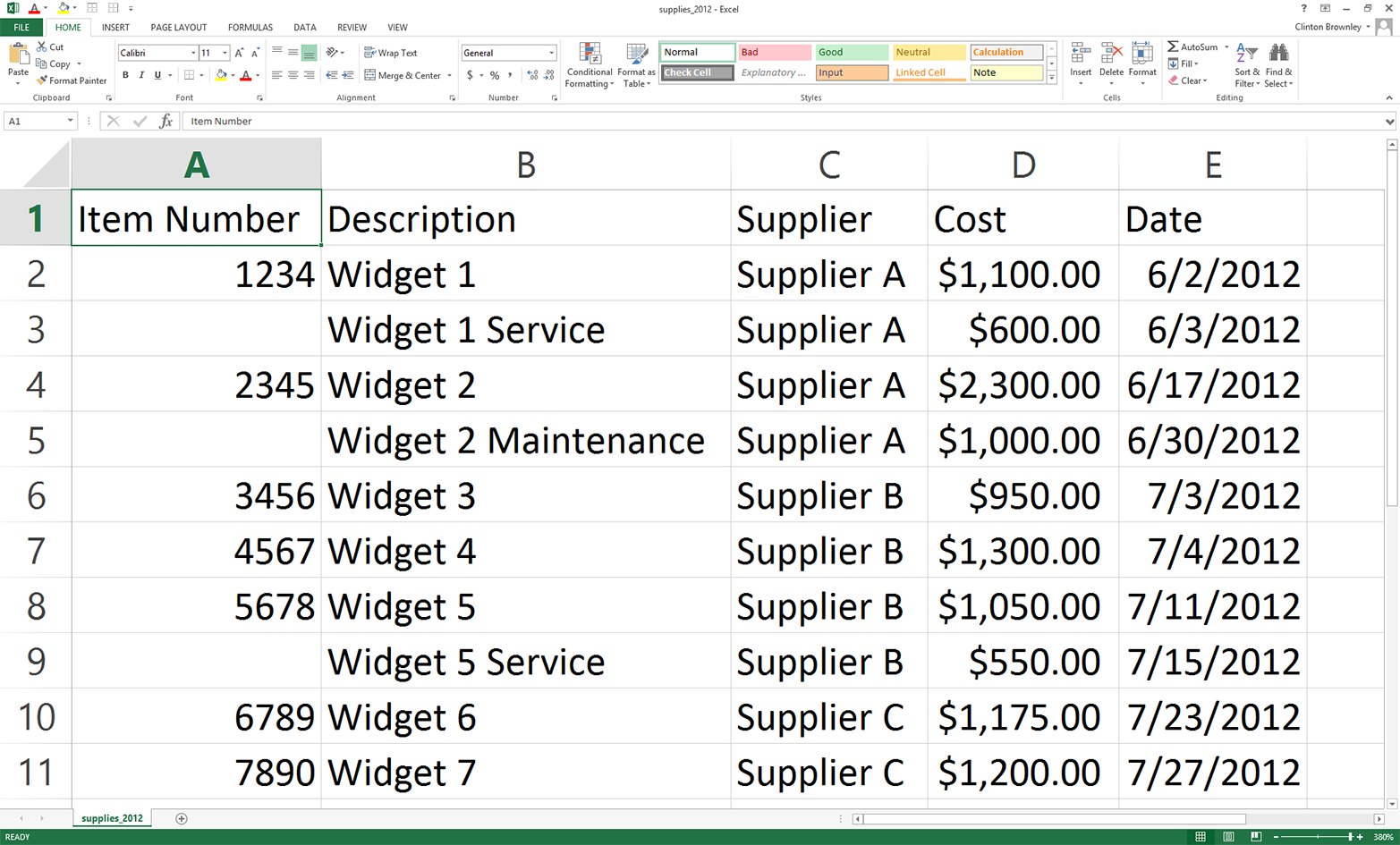
   Figure 5-2. Example data for a CSV file named supplies_2012.csv, displayed in an Excel worksheet

6. Save the file inside the file_archive folder as supplies_2012.csv.

   OK, now we have a CSV file. Next, we need to create an Excel workbook. To do this quickly, let’s use the CSV file we created.

7. In supplies_2012, change the dates in the Date column to 2013 instead of 2012.

   The worksheet should now look as shown in Figure 5-3. As you can see, only the dates have changed.

   

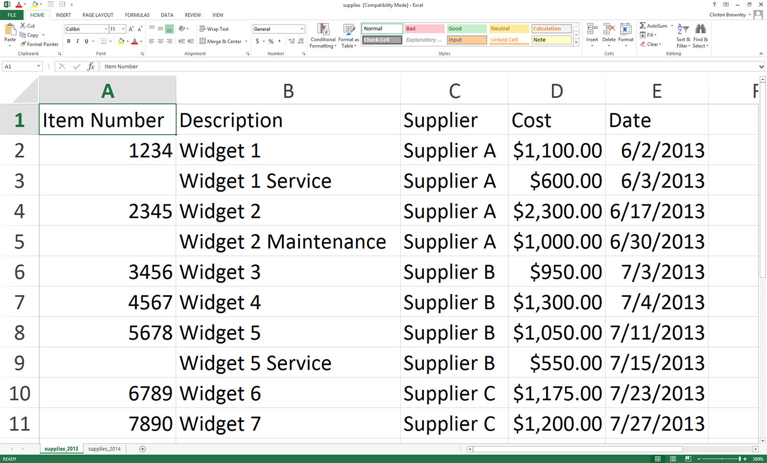
   Figure 5-3. Adding a worksheet for 2013 by changing the dates in supplies_2012 from 2012 to 2013

8. Change the name of the worksheet to supplies_2013.

   To make this file a workbook with multiple worksheets, let’s add a new worksheet.

9. Add a new worksheet by clicking on the + button in the lower-left corner.

10. Name the new worksheet supplies_2014.

11. Copy and paste all of the data from the supplies_2013 worksheet to the supplies_2014 worksheet.

12. Change the dates in the Date column to 2014 instead of 2013.

    The supplies_2014 worksheet should now look as shown in Figure 5-4.

    

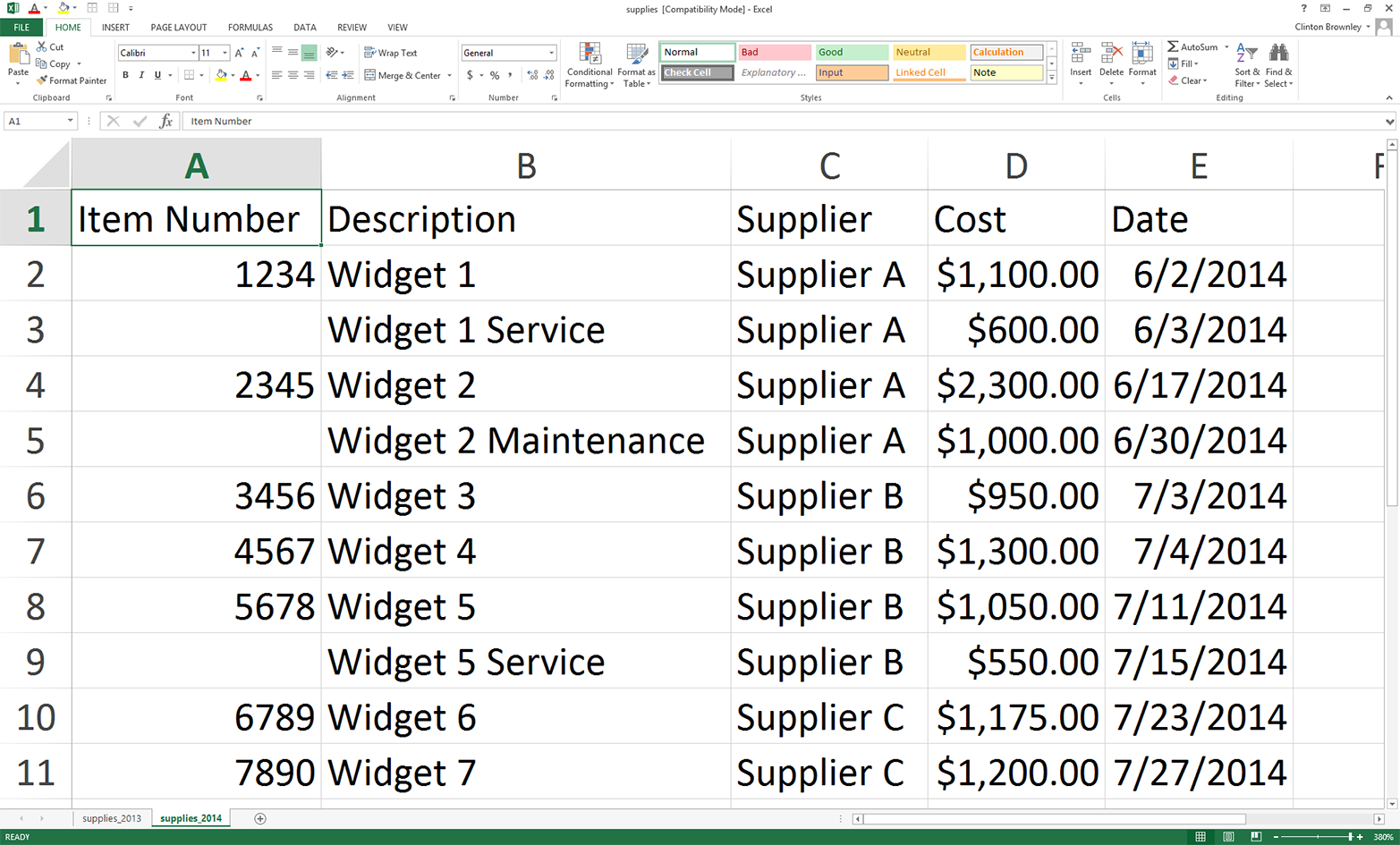
    Figure 5-4. The supplies_2014 worksheet

    As you can see, only the dates have changed—that is, all of the data in the two worksheets is the same, except for the dates in the Date column.

13. Save the Excel file in the file_archive folder as supplies.xls.

14. As a final, optional step, if you can save the file in the Excel Workbook format (.xlsx), reopen the “Save As” dialog box and also save the file as supplies.xlsx.

You should now have three files saved in the file_archive folder:

• A CSV file: supplies_2012.csv

• An Excel file: supplies.xls

• An Excel Workbook file (optional): supplies.xlsx

The example will still work if you could not create the optional .xlsx file, but you’ll have less output. These three files will serve as our set of accumulated historical files, but keep in mind that the code in this example scales to as many CSV and Excel files as your computer can handle.¹ If you have hundreds or thousands of historical CSV or Excel files, you can still use the code in this example as a starting point for your specific search problem, and the code will scale.

Now that we have the folder and files we’re going to search in for the records we want, we need some way to identify the records we’re looking for. In this example, we’ll be searching for specific item numbers. If we were only looking for a few item numbers, we could hardcode them into the Python script as a list or tuple variable (e.g., items_to_look_for = ['1234', '2345']), but this method becomes burdensome or infeasible as the number of items to search for grows. Therefore, we’ll use the method we’ve been using to pass input data into a script and have the item numbers listed in a column in a CSV input file. This way, if you’re looking for a few dozen, hundred, or thousand item numbers, you can list them in a CSV input file and then read that input data into the Python script. This input method scales fairly well, especially compared to hardcoding the values into the Python script.

To list the item numbers that identify the records we’re looking for:

1. Open Excel and add the data shown in Figure 5-5.

2. Save the file as item_numbers_to_find.csv.

As you can see, the five item numbers we’re looking for are 1234, 2345, 4567, 6789, and 7890. They are listed in column A, with no header row. We could include a header row, but it’s unnecessary as we know which column to use and we know the meaning of the data. Plus, if we had a header row we’d have to add some code to process it and remove it because we’re presumably not looking for the header row value in the input files. If in the future another person or program supplies you with this list and it contains a header row, you’ve learned in earlier chapters how to remove it by reading it into a variable and then not using the variable. If you create the list yourself, it makes sense to not include a header row; doing so simplifies the code you need for data processing, and you can recall the meaning of the data based on the filename and the name of the project folder the file is in.

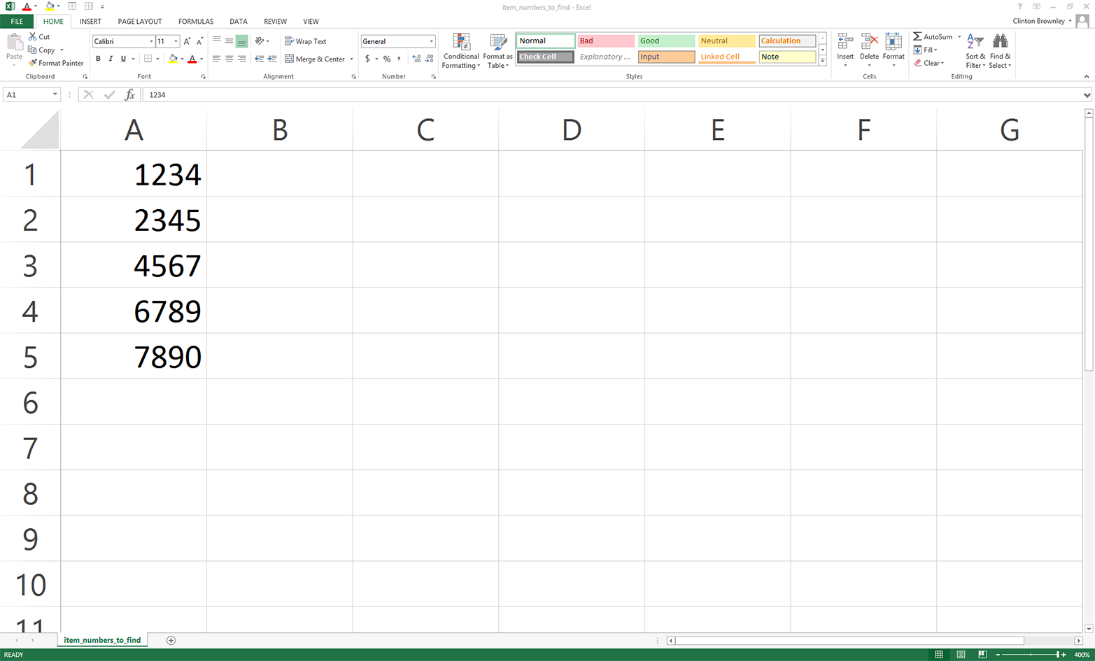
Figure 5-5. Example data for a CSV file named item_numbers_to_find.csv, displayed in an Excel worksheet

At this point, we understand the search task and we have the folder and files we need to carry out the example. To recap, the task is to search in the file_archive folder for files that contain any of the item numbers we’re looking for and, when an item number is found, to write the entire row that contains the item number should be written to an output file. That way, we have all of the historical information associated with the item number available for our discussion with the supplier. We have three historical files in which to search: a CSV file, an Excel file (.xls), and an Excel Workbook file (.xlsx). These three files keep the setup for this example to a minimum, but the code in the script scales and can handle as many input files as your computer can handle. We also have a separate CSV file that contains the item numbers we want to find. We can list hundreds, thousands, or more item numbers in this file, so this input method helps us scale the search as well.

Now that we’ve created the file_archive folder and all of the input files, all we need to do is write some Python code to carry out our search task for us. To do so, type the following code into a text editor and save the file as 1search_for_items_write_found.py:

1 #!/usr/bin/env python3
2 import csv
3 import glob
4 import os
5 import sys
6 from datetime import date
7 from xlrd import open_workbook, xldate_as_tuple
8 item_numbers_file = sys.argv[1]
9 path_to_folder = sys.argv[2]
10 output_file = sys.argv[3]
11 item_numbers_to_find = []
12 with open(item_numbers_file, 'r', newline='') as item_numbers_csv_file:
13     filereader = csv.reader(item_numbers_csv_file)
14     for row in filereader:
15          item_numbers_to_find.append(row[0])
16 #print(item_numbers_to_find)
17 filewriter = csv.writer(open(output_file, 'a', newline=''))
18 file_counter = 0
19 line_counter = 0
20 count_of_item_numbers = 0
21 for input_file in glob.glob(os.path.join(path_to_folder, '*.*')):
22     file_counter += 1
23     if input_file.split('.')[1] == 'csv':
24          with open(input_file, 'r', newline='') as csv_in_file:
25               filereader = csv.reader(csv_in_file)
26               header = next(filereader)
27               for row in filereader:
28                    row_of_output = [ ]
29                    for column in range(len(header)):
30                          if column == 3:
31                               cell_value = str(row[column]).lstrip('$').\
32                               replace(',','').strip()
33                               row_of_output.append(cell_value)
34                          else:
35                               cell_value = str(row[column]).strip()
36                               row_of_output.append(cell_value)
37                    row_of_output.append(os.path.basename(input_file))
38                    if row[0] in item_numbers_to_find:
39                         filewriter.writerow(row_of_output)
40                         count_of_item_numbers += 1
41                    line_counter += 1
42     elif input_file.split('.')[1] == 'xls' or \
43     input_file.split('.')[1] == 'xlsx':
44          workbook = open_workbook(input_file)
45          for worksheet in workbook.sheets():
46               try:
47                    header = worksheet.row_values(0)
48               except IndexError:
49                    pass
50               for row in range(1, worksheet.nrows):
51                    row_of_output = [ ]
52                    for column in range(len(header)):
53                         if worksheet.cell_type(row, column) == 3:
54                              cell_value = \
55                              xldate_as_tuple(worksheet.cell(row,column)\
56                              .value,workbook.datemode)
57                              cell_value = str(date(*cell_value[0:3])).strip()
58                              row_of_output.append(cell_value)
59                         else:
60                              cell_value = \
61                              str(worksheet.cell_value(row,column)).strip()
62                              row_of_output.append(cell_value)
63                    row_of_output.append(os.path.basename(input_file))
64                    row_of_output.append(worksheet.name)
65                    if str(worksheet.cell(row,0).value).split('.')[0].strip() \
66                    in item_numbers_to_find:
67                         filewriter.writerow(row_of_output)
68                         count_of_item_numbers += 1
69                    line_counter += 1
70 print('Number of files:', file_counter)
71 print('Number of lines:', line_counter)
72 print('Number of item numbers:', count_of_item_numbers)

This is a longer script than the ones we wrote in the previous chapter, but if you’ve completed the examples in the preceding chapters then all of the code in this script should look familiar. Lines 2–7 import modules and methods we need to read and manipulate the input data. We import the csv, glob, os, string, and sys modules to read and write CSV files, read multiple files in a folder, find files in a particular path, manipulate string variables, and enter input on the command line, respectively. We import the datetime module’s date method and the xlrd module’s xldate_as_tuple method, as we did in Chapter 3, to ensure that any dates we extract from the input files have a particular format in the output file.

Lines 8, 9, and 10 take the three pieces of input we supply on the command line—the path to and name of the CSV file that contains the item numbers we want to find, the path to the file_archive folder that contains the files in which we want to search, and the path to and name of the CSV output file that will contain rows of information associated with the item numbers found in the historical files—and assign the inputs to three separate variables (item_numbers_file, path_to_folder, and output_file, respectively).

To use the item numbers that we want to find in the code, we need to transfer them from the CSV input file into a suitable data structure like a list. Lines 11–15 accomplish this transfer for us. Line 11 creates an empty list called item_numbers_to_find. Lines 12 and 13 use the csv module’s reader() method to open the CSV input file and create a filereader object for reading the data in the file. Line 14 creates a for loop for looping over all of the rows in the input file. Line 14 uses the list’s append() method to add values to the list we created in line 11. The values added to our list come from the first column, row[0], in the CSV input file. If you want to see the item numbers appended into the list printed to your screen when you run the script, you can uncomment the print statement in line 16.

Line 17 uses the csv module’s writer() method to open a CSV output file in append ('a') mode and creates a filewriter object for writing data to the output file.

Lines 18,19, and 20 create three counter variables to keep track of (a) the number of historical files read into the script, (b) the number of rows read across all of the input files and worksheets, and (c) the number of rows where the item number in the row is one of the item numbers we’re looking for. All three counter variables are initialized to zero.

Line 21 is the outer for loop that loops over all of the input files in the historical files folder. This line uses the os.path.join() function and the glob.glob() function to find all of the files in the file_archive folder that match a specific pattern. The path to the file_archive folder is contained in the variable path_to_folder, which we supply on the command line. The os.path.join() function joins this folder path with all of the names of files in the folder that match the specific pattern expanded by the glob.glob() function. Here, we use the pattern '*.*' to match any filename that ends with any file extension. In this case, because we created the input folder and files, we know the only file extensions in the folder are .csv, .xls, and .xlsx. If instead you only wanted to search in CSV files, then you could use '*.csv'; and if you only wanted to search in .xls or .xlsx files, then you could use '*.xls*'. This a for loop, so the rest of the syntax on this line should look familiar. input_file is a placeholder name for each of the files in the list created by the glob.glob() function.

Line 22 adds one to the file_counter variable for each input file read into the script. After all of the input files have been read into the script, file_counter will contain the total number of files read in.

Line 23 is an if statement that initiates a block of code associated with CSV files. The counterpart of this line is the elif statement in line 42 that initiates a block of code associated with .xls and .xlsx files. Line 23 uses the string module’s split() method to split the path to each input file at the period (.) in the path. For example, the path to the CSV input file is file_archive\supplies_2012.csv. Once this string is split on the period, everything before the period has index [0] and everything after the period has index [1]. This line tests whether the string after the period, with index [1], is csv, which is true for the CSV input file. Therefore, lines 24 to 41 are executed for the CSV input file.

Lines 24 and 25 are familiar. They use the csv module’s reader() method to open the CSV input file and create a filereader object for reading the data in the file.

Line 26 uses the next() method to read the first row of data in the input file, the header row, into a variable called header.

Line 27 creates a for loop for looping through the remaining rows of data in the CSV file. For each of these rows, if the row contains one of the item numbers we’re looking for, then we need to assemble a row of output to write to the output file. To prepare for assembling the row of output, line 28 creates an empty list variable called row_of_output.

Line 29 creates a for loop for looping over each of the columns in a given row in the input file. The line uses the range() and len() functions to create a list of indices associated with the columns in the CSV input file. Because the input file contains five columns, the column variable ranges from 0 to 4.

Lines 30–36 contain an if-else statement that makes it possible to perform different actions on the values in different columns. The if block acts on the column with index 3, which is the fourth column, Cost. For this column, the lstrip() method strips the dollar sign from the lefthand side of the string; the replace() method replaces the comma in the string with no space (effectively deleting the comma); and the strip() method strips any spaces, tabs, and newline characters from the ends of the string. After all of these manipulations, the value is appended into the list; row_of_output in line 37.

The else block acts on the values in all of the other columns. For these values, the strip() method strips any spaces, tabs, and newline characters from the ends of the string, and then the value is appended into the list row_of_output in line 36.

Line 37 appends the basename of the input filename into the list row_of_output. For the CSV input file, the variable input_file contains the string file_archive\supplies_2012.csv. os.path.basename ensures that only supplies_2012.csv is appended into the list row_of_output.

At this point, the first row of data in the CSV input file has been read into the script and each of the column values in the row have been manipulated and then appended into the list row_of_output. Now it is time to test whether the item number in the row is one of the item numbers we want to find. Line 38 carries out this evaluation. The line tests whether the value in the first column in the row, the item number, is in the list of item numbers we want to find, contained in the list variable called item_numbers_to_find. If the item number is one of the item numbers we want to find, then we use the filewriter’s writerow() method in line 39 to write the row of output to our CSV output file. We also add one to the count_of_item_numbers variable in line 40 to keep track of the number of item numbers we found in all of the input files.

Finally, before moving on to the next row of data in the CSV input file, we add one to the line_counter variable in line 41 to keep track of the number of rows of data we found in all of the input files.

The next block of code, in lines 42 through 69 is very similar to the preceding block of code except that it manipulates Excel files (.xls and .xlsx) instead of CSV files. Because the logic in this “Excel” block is the same as the logic in the “CSV” block—the only difference is the syntax for Excel files instead of CSV files—I won’t go into as much detail on every line of code.

Line 42 is an elif statement that initiates a block of code associated with .xls and .xlsx Excel files. Line 42 uses an “or” condition to test whether the file extension is .xls or .xlsx. Therefore, lines 43 to 69 are executed for the .xls and .xlsx Excel input files.

Line 43 uses the xlrd module’s open_workbook() method to open an Excel workbook and assigns its contents to the variable workbook.

Line 44 creates a for loop for looping over all of the worksheets in a workbook. For each worksheet, lines 45 to 48 try to read the first row in the worksheet—the header row—into the variable header. If there is an IndexError, meaning the sequence subscript is out of range, then the Python keyword pass executes and does nothing, and the code continues to line 49.

Line 49 creates a for loop for looping over the remaining data rows in the Excel input file. The range begins at 1 instead of 0 to start at the second row in the worksheet (effectively skipping the header row).

The remaining lines of code in this “Excel” block are basically identical to the code in the “CSV” block, except that they use Excel parsing syntax instead of CSV parsing syntax. The if block acts on the column where the cell type evaluates to 3, which is the column that contains numbers that represent dates. This block uses the xlrd module’s xldate_as_tuple() method and the datetime module’s date() method to make sure the date value in this column retains its date formatting in the output file. Once the value is converted into a text string with date formatting, the strip() method strips any spaces, tabs, and newline characters from the ends of the string and then the list’s append() method appends the value into the list, row_of_output, in line 57.

The else block acts on the values in all of the other columns. For each of these values, the strip() method strips any spaces, tabs, and newline characters from the ends of the string and then the value is appended into the list row_of_output, in line 61.

Line 62 appends the basename of the input filename into the list row_of_output. Unlike CSV files, Excel files can contain multiple worksheets. Therefore, line 63 also appends the name of the worksheet into the list. This additional information for Excel files makes it even easier to see where the script found the item number.

Lines 64–68 are similar to the lines of code for CSV files. Line 64 tests whether the value in the first column in the row, the item number, is in the list of item numbers we want to find, contained in the list variable called item_numbers_to_find. If the item number is one of the item numbers we want to find, then we use the filewriter’s writerow() method in line 66 to write the row of output to our CSV output file. We also add one to the count_of_item_numbers variable in line 67 to keep track of the number of item numbers we found in all of the input files.

Finally, before moving on to the next row of data in the Excel worksheet, we add one to the line_counter variable in line 68 to keep track of the number of rows of data we found in all of the input files.

Lines 69, 70, and 71 are print statements that print summary information to the Command Prompt or Terminal window once the script is finished processing all of the input files. Line 69 prints the number of files processed. Line 70 prints the number of lines read across all of the input files and worksheets. Line 71 prints the number of rows where we found an item number that we were looking for. This count can include duplicates. For example, if item number “1234” appears twice in a single file or once in two separate files, then item number “1234” is counted twice in the value printed to the Command Prompt/Terminal window by this line of code.

Now that we have our Python script, let’s use our script to find specific rows of data in a set of historical files and write the output to a CSV-formatted output file. To do so, type the following on the command line, and then hit Enter:

python 1search_for_items_write_found.py item_numbers_to_find.csv file_archive\
output_files\1app_output.csv

On Windows, you should see the output shown in Figure 5-6 printed to the Command Prompt window.

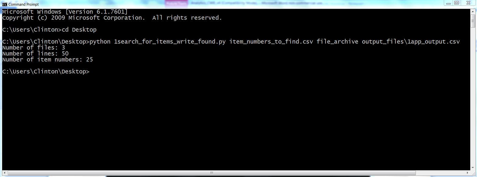
Figure 5-6. The result of running 1search_for_items_write_found.py with item_numbers_to_find.csv and the files in the file_archive folder

As you can see from the output printed to the Command Prompt window, the script read three input files, read 50 rows of data in the input files, and found 25 rows of data associated with the item numbers we wanted to find. This output doesn’t show how many of the item numbers were found or how many copies of each of the item numbers were found. However, that is why we wrote the output to a CSV output file.

To view the output, open the output file named 1app_output.csv. The contents should look as shown in Figure 5-7.

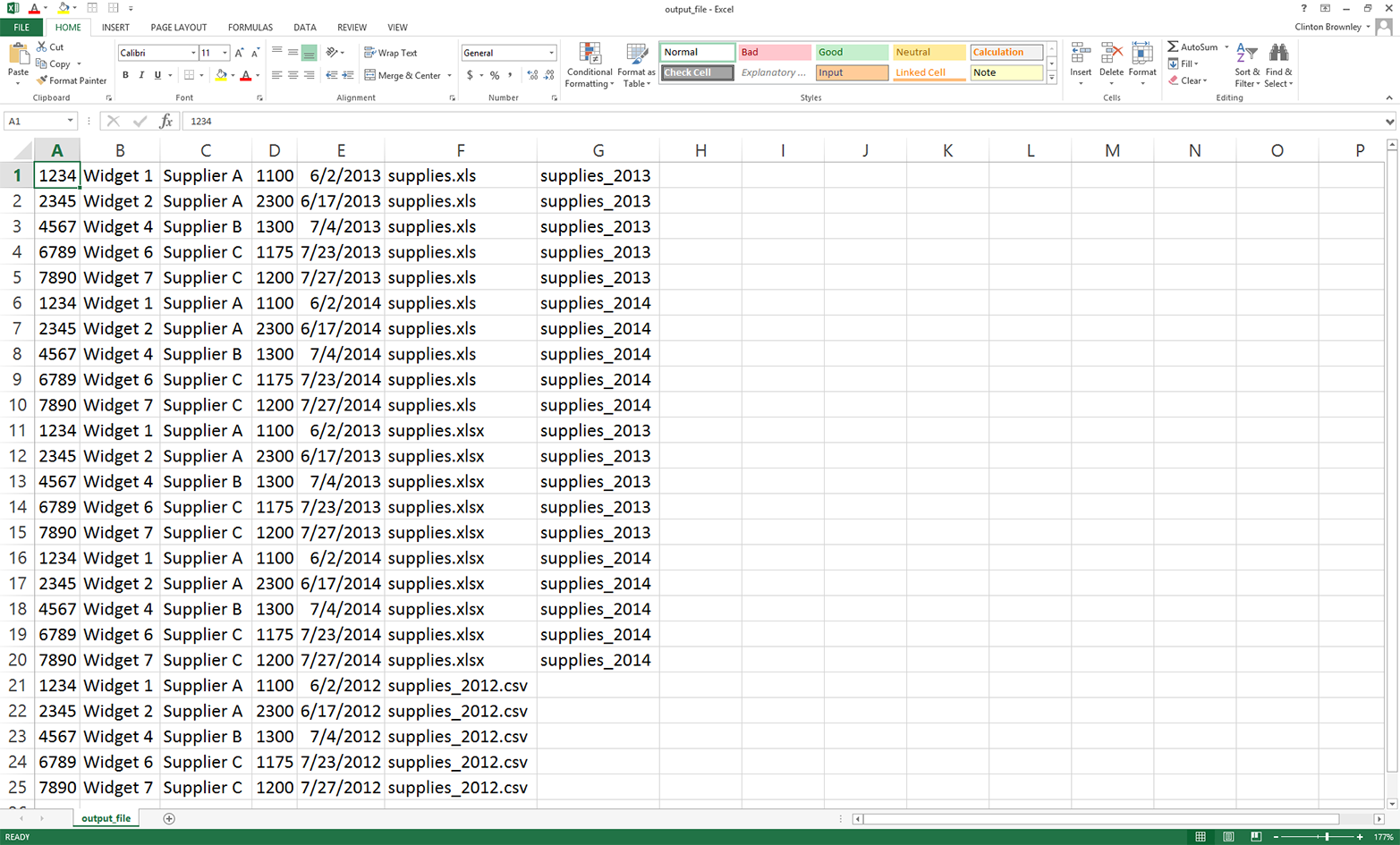
Figure 5-7. The data that 1search_for_items_write_found.py wrote into 1app_output.csv

These records are the rows in the three input files that have item numbers matching those listed in the CSV file. The second-to-last column lists the names of the files where the data is found. The last column lists the names of the worksheets where the data is found in the two Excel workbooks.

As you can see from the contents of this output file, we found 25 rows of data associated with the item numbers we wanted to find. This output is consistent with the “25” that was printed to the Command Prompt window. Specifically, we found each of the five item numbers we wanted to find five times across all of the input files. For example, item number “1234” was found twice in the .xls file (once in the supplies_2013 worksheet and once in the supplies_2014 worksheet), twice in the .xlsx file (once in the supplies_2013 worksheet and once in the supplies_2014 worksheet), and once in the CSV input file.

Compared to the rows that came from the CSV input file, the rows of output that came from the Excel workbooks have an additional column (i.e., the name of the worksheet in which the row of data was found). The costs in the fourth column only include the dollar portion of the cost amount from the input files. Finally, the dates in the fifth column are formatted consistently across the CSV and Excel input files.

This application combined several of the techniques we learned in earlier chapters to tackle a common, real-world problem. Business analysts often run into the problem of needing to assemble historical data spread across multiple files and file types into a single dataset. In many cases, there are dozens, hundreds, or thousands of historical files and the thought of having to search for and extract specific data from these files is daunting.

In this section, we demonstrated a scalable way to extract specific records from a set of historical records. To keep the setup to a minimum, the example only included a short list of item numbers and three historical records. However, the method scales well, so you can use it to search for a longer list of items and in a much larger collection of files.

Now that we’ve tackled the problem of searching for specific records in a large collection of historical files, let’s turn to the problem of calculating a statistic for an unknown number of categories. This objective may sound a bit abstract right now, but let’s turn to the next section to learn more about this problem and how to tackle it.

Calculate a Statistic for Any Number of Categories from Data in a CSV File

Many business analyses involve calculating a statistic for an unknown number of categories in a specific period of time. For example, let’s say you sell five different products and you want to calculate the total sales by product category for all of your customers in a specific year. Because your customers have different tastes and preferences, they have purchased different products throughout the year. Some of your customers have purchased all five of your products; others have only purchased one of your products. Given your customers’ purchasing habits, the number of product categories associated with each customer differs across customers.

To make it easy, you could associate all five product categories with each of your customers, initiate total sales for all of the product categories at zero, and only increase the total sales amounts for the products each customer has actually purchased. However, we already know that many customers have only purchased one or two products, and you’re only interested in the total sales for the products that customers have actually purchased. Associating all five product categories with all of your customers is excessive, distracting, and wasteful of memory, computing resources, and storage space. For these reasons, it makes sense to only capture the data you need—for each customer, the products they purchased and the total sales in each of the product categories.

As another example, imagine that your customers progress through different product or service packages over time. For example, you supply a Bronze package, a Silver package, and a Gold package. Some customers buy the Bronze package first, some buy the Silver package first, and some buy the Gold package first. For those customers who buy the Bronze or Silver package first, they tend to progress to higher-value packages over time.

You are interested in calculating the total amount of time, perhaps in months, that your customers have spent in each of the package categories they’ve purchased. For example, if one of your customers, Tony Shephard, purchased the Bronze package on 2/15/2014, purchased the Silver package on 6/15/2014, and purchased the Gold package on 9/15/2014, then the output for Tony Shepard would be “Bronze package : 4 months”; “Silver package : 3 months”; and “Gold package: the difference between today’s date and 9/15/2014”. If a different customer, Mollie Adler, has only purchased the Silver and Gold packages, then the output for Mollie Adler would not include any information on the Bronze package.

If the dataset on your customers is small enough, then you could open the file, calculate the differences between the dates, and then aggregate them by package category and customer name. However, this manual approach would be time consuming and error prone. And what happens if the file is too large to open? This application is an excellent opportunity to use Python. Python can handle files that are too large to open, it performs the calculations quickly, and it reduces the chance of human errors.

In order to perform calculations on a dataset of customer package purchases, we need to create a CSV file with the data:

1. Open Excel and add the data shown in Figure 5-8.

   

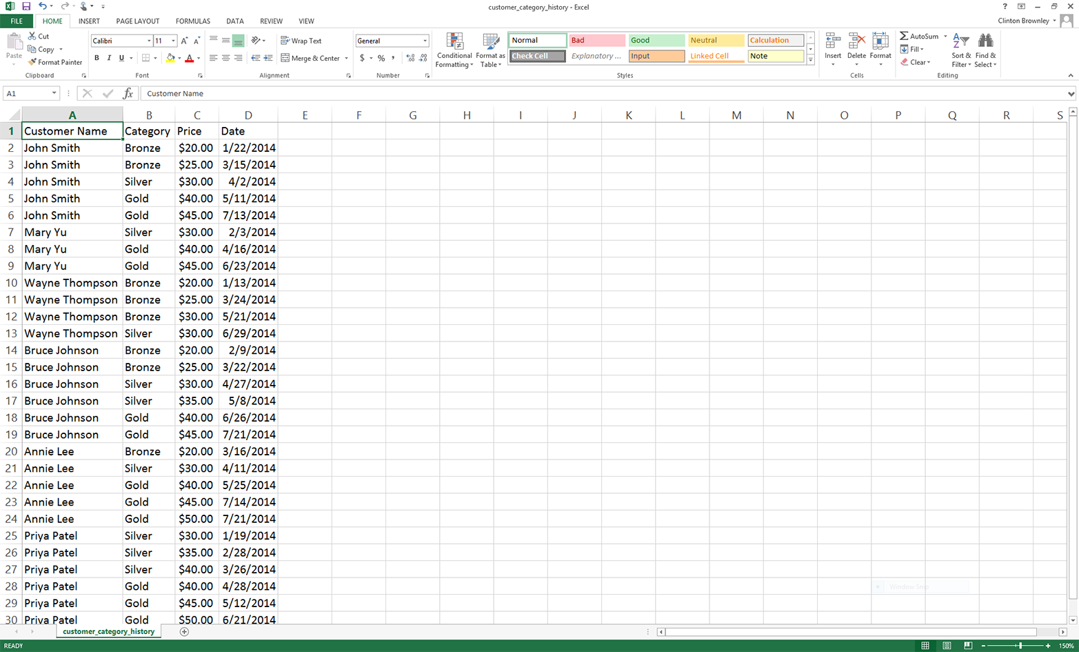
   Figure 5-8. Example data for a CSV file named customer_category_history.csv, displayed in an Excel worksheet

2. Save the file as customer_category_history.csv.

As you can see, this dataset includes four columns: Customer Name, Category, Price, and Date. It includes six customers: John Smith, Mary Yu, Wayne Thompson, Bruce Johnson, Annie Lee, and Priya Patel. It includes three package categories: Bronze, Silver, and Gold. The data is arranged by Customer Name and then by Date, ascending.

Now that we have our dataset on the packages our customers have purchased over the past year and the dates on which the packages were purchased or renewed, all we need to do is write some Python code to carry out our binning and calculation tasks for us.

To do so, type the following code into a text editor and save the file as 2calculate_statistic_by_category.py:

1 #!/usr/bin/env python3
2 import csv
3 import sys
4 from datetime import date, datetime
5 
6 def date_diff(date1, date2):
7     try:
8          diff = str(datetime.strptime(date1, '%m/%d/%Y') - \
9          datetime.strptime(date2, '%m/%d/%Y')).split()[0]
10     except:
11          diff = 0
12     if diff == '0:00:00':
13          diff = 0
14     return diff
15 input_file = sys.argv[1]
16 output_file = sys.argv[2]
17 packages = { }
18 previous_name = 'N/A'
19 previous_package = 'N/A'
20 previous_package_date = 'N/A'
21 first_row = True
22 today = date.today().strftime('%m/%d/%Y')
23 with open(input_file, 'r', newline='') as input_csv_file:
24     filereader = csv.reader(input_csv_file)
25     header = next(filereader)
26     for row in filereader:
27          current_name = row[0]
28          current_package = row[1]
29          current_package_date = row[3]
30          if current_name not in packages:
31               packages[current_name] = { }
32          if current_package not in packages[current_name]:
33               packages[current_name][current_package] = 0
34          if current_name != previous_name:
35               if first_row:
36                    first_row = False
37               else:
38                    diff = date_diff(today, previous_package_date)
39                    if previous_package not in packages[previous_name]:
40                         packages[previous_name][previous_package] = int(diff)
41                    else:
42                         packages[previous_name][previous_package] += int(diff)
43          else:
44               diff = date_diff(current_package_date, previous_package_date)
45               packages[previous_name][previous_package] += int(diff)
46          previous_name = current_name
47          previous_package = current_package
48          previous_package_date = current_package_date
49 header = ['Customer Name', 'Category', 'Total Time (in Days)']
50 with open(output_file, 'w', newline='') as output_csv_file:
51     filewriter = csv.writer(output_csv_file)
52     filewriter.writerow(header)
53     for customer_name, customer_name_value in packages.items():
54          for package_category, package_category_value \
55          in packages[customer_name].items():
56               row_of_output = [ ]
57               print(customer_name, package_category, package_category_value)
58               row_of_output.append(customer_name)
59               row_of_output.append(package_category)
60               row_of_output.append(package_category_value)
61               filewriter.writerow(row_of_output)

The code in this script accomplishes the calculation task, but it is also interesting and educational—it is the first example in this book to use Python’s dictionary data structure to organize and store our results. In fact, the example in this script is more complicated than a simple dictionary because it involves a nested dictionary, a dictionary within a dictionary. This example shows how convenient it can be to create a dictionary and to fill it with key-value pairs. In this example, the outer dictionary is called packages. The outer key is the customer’s name. The value associated with this key is another dictionary, where the key is the name of the package category and the value is an integer that captures the number of days the customer has had the specific package. Dictionaries are handy data structures to understand, because many data sources and analyses lend themselves to the key-value pair structure. As you’ll recall from Chapter 1, dictionaries are created with curly braces ({}), the keys in a dictionary are unique strings, the keys and values in a key-value pair are separated by colons, and each of the key-value pairs are separated by commas—for example, costs = {'people': 3640, 'hardware': 3975}.

In addition, this script demonstrates how to handle the first row of data about a particular category differently from all of the remaining rows about that category in order to calculate statistics based on differences between the rows. For example, in the script, all of the code in the outer if statement, if current_name != previous_name, is only executed for the first row of data about a new customer. All of the remaining rows about the customer enter into the outer else statement.

Finally, this script demonstrates how to define and use a user-defined function. The function in this script, date_diff, calculates and returns the amount of time in days between two dates. The function is defined in lines 6–14, and is used in lines 40 and 47. If we didn’t define a function, the code in the function would have to be repeated twice in the script, first at line 38 and again at line 44. By defining a function, you only have to write the code once, you reduce the number of lines of code in the script, and you simplify the code that appears in lines 40 and 47. As mentioned in Chapter 1, whenever you notice that you are repeating code in your script, consider bundling the code into a function and using the function to simplify and shorten the code in your script.

Now that we have covered some of the notable aspects of the script, let’s discuss specific lines of code. Lines 2–5 import modules and methods we need to read and manipulate the input data. We import the csv, datetime, string, and sys modules to read and write CSV files, manipulate date variables, manipulate string variables, and enter input on the command line, respectively. From the datetime module, we import the date and datetime methods to access today’s date and calculate differences between dates.

Lines 6–14 define the user-defined date_diff function. Line 6 contains the definition statement, which names the function and shows that the function takes two values, date1 and date2, as arguments to the function. Lines 7–11 contain a try-except error handling statement. The try block attempts to create datetime objects from date strings with datetime.strptime(), subtract the second date from the first date, convert the result of the subtraction into a string with str(), split the resulting string on whitespace with split(), and finally retain the leftmost portion of the split string (the string with index [0]) and assign it to the variable diff. The except block executes if the try block encounters any errors. If that happens, the except block sets diff to the integer zero. Similarly, lines 12 and 13 are an if statement that handles the situation when the two dates being processed are equal and therefore the difference between the dates is zero, formatted as '0:00:00'. If the difference evaluates to zero (note the two equals signs), then the if statement sets diff to the integer zero. Finally, in line 14 the function returns the integer value contained in the variable diff.

Lines 15 and 16 take the two pieces of input we supply on the command line—the path to and name of the CSV input file that contains our customer data, and the path to and name of the CSV output file that will contain rows of information associated with our customers and how long they’ve had particular packages—and assign the inputs to two separate variables (input_file and output_file, respectively.)

Line 17 creates an empty dictionary called packages that will contain the information we want to retain. Lines 18, 19, and 20 create three variables, previous_name, previous_package, and previous_package_date, and assign each of them the string value 'N/A'. We assign the value 'N/A' to these variables assuming the string 'N/A' does not appear anywhere in the three columns of customer names, package categories, or package dates in the input file. If you plan to modify this code for your own analysis and the column you’re using for your dictionary keys includes the string 'N/A', then change 'N/A' to a different string that doesn’t appear in your column in your input file—'QQQQQ' or something equally distinctive yet meaningless works.

Line 21 creates a Boolean variable called first_row and assigns it the value, True. We use this variable to determine whether we’re processing the first row of data in the input file. If we are processing the first row of data, then we process it with one block of code. If we’re not processing the first row, then we use another block of code.

Line 22 creates a variable called today that contains today’s date, formatted as %m/%d/%Y. With this format, a date like October 21, 2014 appears as 10/21/2014.

Lines 23 and 24 use a with statement and the csv module’s reader method to open the CSV input file and create a filereader object for reading the data in the file. Line 25 uses the next method on the filereader object to read the first row from the input file and assigns the list of values to the variable header.

Line 26 creates a for loop for looping over all of the remaining data rows in the input file. Line 27 captures the value in the first column, row[0], and assigns it to the variable current_name. Line 28 captures the value in the second column, row[1], and assigns it to the variable current_package. Line 29 captures the value in the fourth column, row[3], and assigns it to the variable current_package_date. The first data row contains the values John Smith, Bronze, and 1/22/2014, so these are the values assigned to current_name, current_package, and current_package_date, respectively.

Line 30 creates an if statement to test whether the value in the variable current_name is not already a key in the packages dictionary. If it is not, then line 31 adds the value in current_name as a key in the packages dictionary and sets the value associated with the key as an empty dictionary. These two lines serve to populate the packages dictionary with its collection of key-value pairs.

Similarly, line 32 creates an if statement to test whether the value in the variable current_package is not already a key in the inner dictionary associated with the customer name contained in the variable current_name. If it is not, then line 33 adds the value in current_package as a key in the inner dictionary and sets the value associated with the key as the integer zero. These two lines serve to populate the key-value pairs in the inner dictionary associated with each customer name.

For example, in line 31, John Smith becomes a key in the packages dictionary, and the associated value is an empty dictionary. In line 33, the first package category associated with John Smith (i.e., Bronze), becomes a key in the inner dictionary and the value associated with Bronze is initialized to zero. At this point, the packages dictionary looks like: {'John Smith': {'Bronze': 0}}.

Line 34 creates an if statement to test whether the value in the variable current_name does not equal the value in the variable previous_name. The first time we reach this line in the script, the value in current_name is the first customer name in our input file (i.e., John Smith). The value in previous_name is 'N/A'. Because John Smith doesn’t equal 'N/A', we enter the if statement.

Line 35 creates an if statement to test whether the code is processing the first row of data in the input file. Because the variable first_row currently has the value True, line 35 executes line 36, which assigns the variable first_row the value False.

Next, the script moves on to lines, 46, 47, and 48 to assign the values in the three variables current_name, current_package, and current_package_date to the three variables previous_name, previous_package, and previous_package_date, respectively. Therefore, previous_name now contains the value John Smith, previous_package now contains the value Bronze, and previous_package_date now contains the value 1/22/2014.

At this point, the script has finished processing the first row of data in the input file, so the script returns to line 26 to process the next row of data in the file. For this data row, lines 27, 28, and 29 assign the values in the first, second, and fourth columns in the row to the variables current_name, current_package, and current_package_date, respectively. Because the second row of data contains the values John Smith, Bronze, and 3/15/2014, these are now the values contained in current_name, current_package, and current_package_date.

Line 30 once again tests whether the value in the variable current_name is not already a key in the packages dictionary. Because John Smith is already a key in the dictionary, line 31 is not executed. Similarly, line 32 once again tests whether the value in the variable current_package is not already a key in the inner dictionary. Bronze is already a key in the inner dictionary, so line 33 is not executed.

Next, line 34 tests whether the value in current_name is not equal to the value in previous_name. The value in current_name is John Smith and the value in previous_name is also John Smith. Because the values in the two variables are equal, lines 35 to 42 are skipped and we move on to the else block that starts at line 43.

Line 44 uses the user-defined date_diff function to subtract the value in previous_package_date from the value in current_package_date and assigns the value (in days) to the variable diff. We’re processing the second data row in the input file, so the value in current_package_date is 3/15/2014. In the previous loop we assigned the value 1/22/2014 to the variable previous_package_date. Therefore, the value in diff is 3/15/2014 minus 1/22/2014, or 52 days.

Line 45 increments the amount of time a specific customer has had a specific package by the value in diff. For example, this time through the loop the value in previous_name is John Smith and the value in previous_package is Bronze. Therefore, we increment the amount of time John Smith has had the Bronze package from zero to 52 days. At this point, the packages dictionary looks like: {'John Smith': {'Bronze': 52}}. Note that the value has increased from 0 to 52.

Finally, lines 46, 47, and 48 assign the values in current_name, current_package, and current_package_date to the variables previous_name, previous_package, and previous_package_date, respectively.

To make sure you understand how the code is working, let’s discuss one more iteration through the loop. In the previous paragraph we noted that the three previous_* variables were assigned the values in the three current_* variables. So the values in previous_name, previous_package, and previous_package_date are now John Smith, Bronze, and 3/15/2014, respectively. In the next iteration through the loop, lines 27, 28, and 29 assign the values in the third data row of the input file to the three current_* variables. After the assignments, the values in current_name, current_package, and current_package_date are now John Smith, Silver, and 4/2/2014, respectively.

Line 30 once again tests whether the value in the variable current_name is not already a key in the packages dictionary. John Smith is already a key in the dictionary, so line 31 is not executed.

Line 32 tests whether the value in the variable current_package is not already a key in the inner dictionary. This time, the value in current_package, Silver, is new; it is not already a key in the inner dictionary. Because Silver is not a key in the inner dictionary, line 33 makes Silver a key in the inner dictionary and initializes the value associated with Silver to zero. At this point, the packages dictionary looks like: {'John Smith': {'Silver': 0, 'Bronze': 52}}.

Next, line 34 tests whether the value in current_name is not equal to the value in previous_name. The value in current_name is John Smith and the value in previous_name is also John Smith. The values in the two variables are equal, so lines 35 to 42 are skipped and we move on to the else block that starts at line 43.

Line 44 uses the user-defined date_diff function to subtract the value in previous_package_date from the value in current_package_date and assigns the value (in days) to the variable diff. Because we’re processing the third data row in the input file, the value in current_package_date is 4/2/2014. In the previous loop we assigned the value 3/15/2014 to the variable previous_package_date. Therefore, the value in diff is 4/2/2014 minus 3/15/2014, or 18 days.

Line 45 increments the amount of time a specific customer has had a specific package by the value in diff. For example, this time through the loop the value in previous_name is John Smith and the value in previous_package is Bronze. Therefore, we increment the amount of time John Smith has had the Bronze package from 52 to 70 days. At this point, the packages dictionary looks like: {'John Smith': {'Silver': 0, 'Bronze': 70}}.

Again, lines 46, 47, and 48 assign the values in current_name, current_package, and current_package_date to the variables previous_name, previous_package, and previous_package_date, respectively.

Once the for loop has finished processing all of the rows in the input file, lines 49 to 61 write a header row and the contents of the nested dictionary to an output file. Line 49 creates a list variable called header that contains three string values, Customer Name, Category, and Total Time (in Days), which will be the headers for the three columns in the output file.

Lines 50 and 51 open an output file for writing and create a writer object for writing to the output file, respectively. Line 52 writes the contents of header, the header row, to the output file.

Lines 53 and 54 are for loops for looping through the keys and values of the outer and inner dictionaries, respectively. The keys in the outer dictionary are the customer names. The value associated with each customer name is another dictionary. The keys in the inner dictionary are the categories of the packages the customer has purchased. The values in the inner dictionary are the amounts of time (in days) the customer has had each of the packages.

Line 56 creates an empty list, called row_of_output, that will contain the three values we want to output for each line in the output file. Line 57 prints these three values for each row of output so we can see the output that will be written to the output file. You can remove this line once you’re confident the script is working as expected. Lines 58 to 60 append the three values we want to output into the list, row_of_output. Finally, for every customer name and associated package category in the nested dictionary, line 61 writes the three values of interest to the output file in comma-delimited format.

Now that we have our Python script, let’s use our script to calculate the amount of time each customer has had different package categories and write the output to a CSV-formatted output file. To do so, type the following on the command line, and then hit Enter:

python 2calculate_statistic_by_category.py customer_category_history.csv\
output_files\2app_output.csv

You should see output similar to what is shown in Figure 5-9 printed to the Command Prompt or Terminal window (the exact numbers you see for each person will be different because you’re using today’s date in the script).

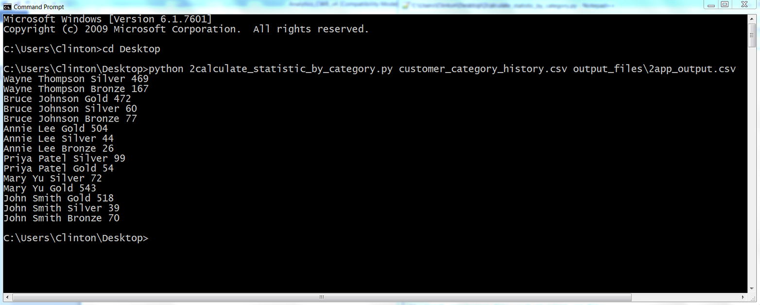
Figure 5-9. The result of running 2calculate_statistic_by_category.py on the CSV file named customer_category_history.csv

The output shown in the Command Prompt window reflects the output that was also written to 2app_output.csv. The contents of the file should look Figure 5-10. It shows the number of days each customer has had a specific package.

As you can see, the script wrote the header row to the output file and then wrote a row for every unique pair of customer names and package categories it processed from the input file. For example, the first two data rows beneath the header row show that Wayne Thompson had the Bronze package for 167 days and the Silver package for 469 days. The last three rows show that John Smith had the Bronze package for 70 days, the Silver package for 39 days, and the Gold package for 518 days. The remaining data rows show the results for the other customers. Having processed and aggregated the raw data in the input file, you can now calculate additional statistics with this data, summarize and visualize the data in different ways, or combine the data with other data for further analyses.

One note to point out is the business decision (a.k.a. assumption) we made about how to deal with the last package category for each customer. Presumably, if our input data is accurate and up to date, then the customer still has the last package category we have on record for the customer. For example, the last package category for Wayne Thompson is Silver, purchased on 6/29/2014. Because Wayne Thompson presumably still has this package, the amount of time assigned to this package should be the amount of time between today’s date and 6/29/2014, which means the amount of time added to the final package category for each customer depends on when you run the script.

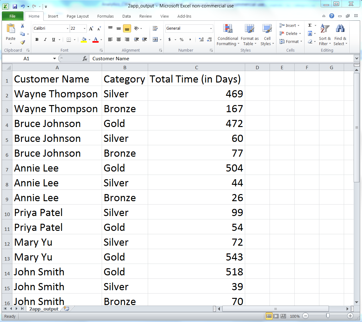
Figure 5-10. The output of 2calculate_statistic_by_category.py (i.e., the number of days each customer has had a specific package) in a CSV file named 2app_output.csv, displayed in an Excel worksheet

The code that implements this calculation and addition appears indented beneath line 34. Line 34 ensures that we do not try to calculate a difference for the first row of data, as we can’t calculate a difference based on one date. After processing the first row, line 35 sets first_row equal to False. Now, for all of the remaining data rows, line 35 is False, line 36 is not executed. For each transition from one customer to the next, lines 38 to 42 are executed. Line 38 calculates the difference (in days) between today’s date and the value in previous_package_date and assigns the integer value to the variable diff. Then, if the value in previous_package is not already a key in the inner dictionary, line 40 makes the value in previous_package a key in the inner dictionary and sets the associated value to the integer in diff. Alternatively, if the value in previous_package is already a key in the inner dictionary, then line 42 adds the integer in diff to the existing integer value associated with the corresponding key in the inner dictionary.

Returning to the Wayne Thompson example, the last package category for Wayne Thompson is Silver, with a purchse date of 6/29/2014. The next row of input data is for a different customer, Bruce Johnson, so the code beneath line 34 is executed. Running the script at the time I was writing this chapter, on 10/11/2015, resulted in the value in diff being 10/11/2015 minus 6/29/2014, or 469 days. As you can see in the Command Prompt window and in the output file shown previously, the amount of time recorded for Wayne Thompson and the Silver category is 469 days.

If you run this script on a different day, then the amount of time in this row of output, and all of the rows of output corresponding to each customer’s last package category, will be different (i.e., they should be larger numbers). How to deal with the last row of data for each customer is a business decision. You can always modify the code in this example to reflect how you want to treat the row for your specific use case.

This application combined several of the techniques we learned in Chapter 1, such as creating a user-defined function and populating a dictionary, to tackle a common, real-world problem. Business analysts often run into the problem of needing to calculate differences between values in rows of input data. In many cases, there are thousands or millions of rows that need to be handled in different ways, and the thought of having to calculate differences for particular rows manually is daunting (if the task is even possible).

In this section, we demonstrated a scalable way to calculate differences between values in rows and aggregate the differences based on values in other columns in the input file. To keep the setup to a minimum, the example only included a short list of customer records. However, the method scales well, so you can use it to perform calculations for a longer list of records or modify the code to process data from multiple input files.

Now that we’ve tackled the problem of calculating a statistic for an unknown number of categories, let’s turn to the problem of parsing a plain-text file for key pieces of data. This problem may sound a bit abstract right now, but let’s turn to the next section to learn more about this problem and how to tackle it.

Calculate Statistics for Any Number of Categories from Data in a Text File

The previous two applications demonstrated how to accomplish specific tasks with data in CSV and Excel files. Indeed, the majority of this book has focused on parsing and manipulating data in these files. For CSV files, we’ve used Python’s built-in csv module. For Excel files, we downloaded and have used the xlrd add-in module. CSV and Excel files are common file types in business, so it is important to understand how to deal with them.

At the same time, text files (a.k.a. flat files) are also a common file type in business. In fact, we already discussed how CSV files are actually stored as comma-delimited text files. A few more common examples of business data stored in text files are activity logs, error logs, and transaction records. Because text files, like CSV and Excel files, are common in business, and up to this point we haven’t focused on parsing text files, we’ll use this application to demonstrate how to extract data from text files and calculate statistics based on the data.

As mentioned in the previous paragraph, error logs are often stored in text files. The MySQL database system is one system that stores its error log as a text file. We downloaded and used the MySQL database system in the previous chapter, so if you followed along with the examples in the chapter, then you can access your MySQL system’s error log file. Keep in mind, however, that locating and viewing your MySQL system’s error log file is for your own edification; you do not have to access it to follow along with the example in this section.

To access your MySQL system’s error log file on Windows, open File Explorer, open the C: drive, open ProgramData, open the MySQL folder, open the MySQL Server <Version> folder (e.g., MySQL Server 5.6), and finally open the data folder. Inside the data folder, there should be an error log file that ends with the file extension .err. Right-click the file and open it with a text editor like Notepad or Notepad++ to view the errors your MySQL system has already written to the log file. If you cannot find one of the folders in this path, open File Explorer, open the C: drive, type “.err” in the search box in the upper-right corner, and wait for your system to find the error file. If your system finds many error files, then select the one with a path that is most similar to the one described above.

Because the data in your MySQL error log file is undoubtedly different from the data in my MySQL error log file, we’ll use a separate, representative MySQL error log file in this application. That way we can focus on the Python code instead of the idiosyncrasies of our different error log files. To create a typical MySQL error log file for this application, open a text editor, write the lines of text shown in Figure 5-11, and save the file as mysql_server_error_log.txt.

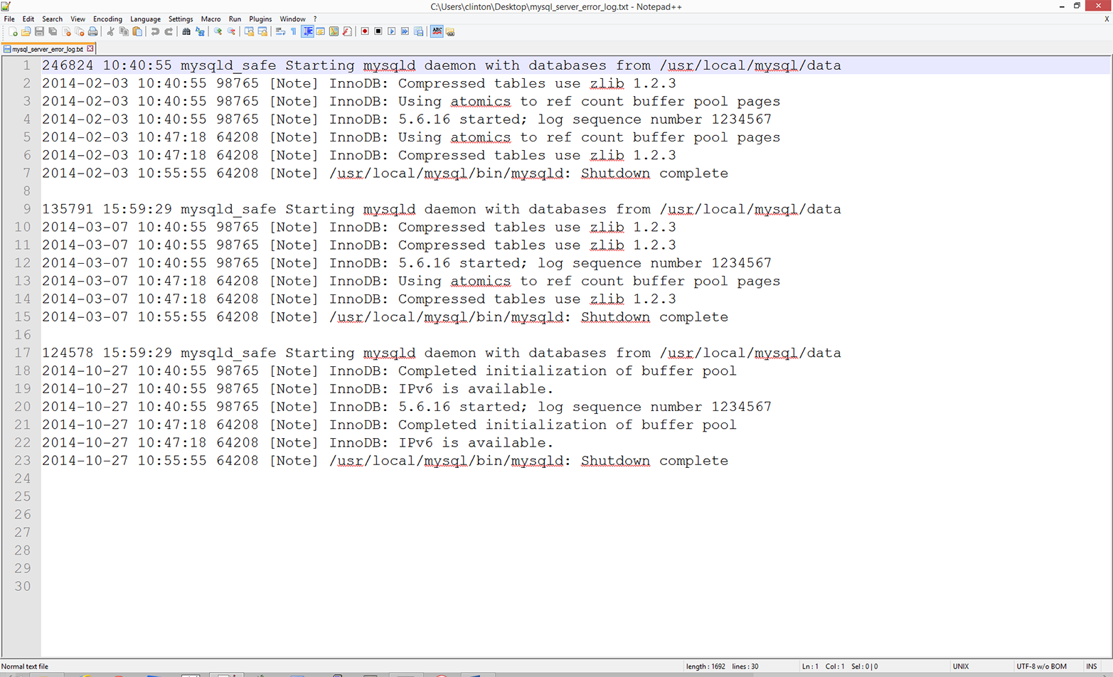
Figure 5-11. Example MySQL database error log data for a text file named mysql_server_error_log.txt, displayed in Notepad++

As you can see, a MySQL error log file contains information on when mysqld was started and stopped and also any critical errors that occurred while the server was running. For example, the first line in the file shows when mysqld was started and the seventh line shows when mysqld was stopped on that day. Lines 2–6 show the critical errors that occurred while the server was running on that day. These lines begin with a date and timestamp, and the critical error message is preceded by the term [Note]. The remaining lines in the file contain similar information for different days.

To reduce the amount of writing you need to do to create the file, I’ve repeated the timestamps and many of the critical error messages. Therefore, to create the file you really only need to write lines 1–7, copy and paste those lines twice, and then modify the dates and error messages.

Now that we have our MySQL error log text file, we need to discuss the business application. Text files like the one in this application often store disaggregated data, which can be parsed, aggregated, and analyzed for potential insights. For example, in this application, the error log file has recorded the types of errors that have occurred and when they have occurred. In its native layout, it is difficult to discern whether specific errors occur more frequently than other errors and whether the frequency of particular errors is changing over time. By parsing the text file, aggregating relevant pieces of data, and writing the output in a useful format, we can gain insights from the data that can drive corrective actions. The text files that you use may not be MySQL error logs, but being able to parse text files for key pieces of data and aggregate the data to generate insights is a skill that is generally applicable across text files.

Now that we understand the business application, all we need to do is write some Python code to carry out our error message binning and calculation tasks. To do so, type the following code into a text editor and save the file as 3parse_text_file.py:

1 #!/usr/bin/env python3
2 import sys
3 
4 input_file = sys.argv[1]
5 output_file = sys.argv[2]
6 messages = { }
7 notes = [ ]
8 with open(input_file, 'r', newline='') as text_file:
9     for row in text_file:
10          if '[Note]' in row:
11               row_list = row.split(' ', 4)
12               day = row_list[0].strip()
13               note = row_list[4].strip('\n').strip()
14               if note not in notes:
15                    notes.append(note)
16               if day not in messages:
17                    messages[day] = { }
18               if note not in messages[day]:
19                    messages[day][note] = 1
20               else:
21                    messages[day][note] += 1
22 filewriter = open(output_file, 'w', newline='')
23 header = ['Date']
24 header.extend(notes)
25 header = ','.join(map(str,header)) + '\n'
26 print(header)
27 filewriter.write(header)
28 for day, day_value in messages.items():
29     row_of_output = [ ]
30     row_of_output.append(day)
31     for index in range(len(notes)):
32          if notes[index] in day_value.keys():
33               row_of_output.append(day_value[notes[index]])
34          else:
35               row_of_output.append(0)
36     output = ','.join(map(str,row_of_output)) + '\n'
37     print(output)
38     filewriter.write(output)
39 filewriter.close()

Because we are parsing a text file containing plain text in this application, instead of a CSV or Excel file, we do not need to import the csv or xlrd modules. We only need to import Python’s built-in string and sys modules, which we import in lines 2 and 3. As described previously, these two modules enable us to manipulate strings and read input from the command line, respectively.

Lines 4 and 5 take the two pieces of input we supply on the command line—the path to and name of the input text file that contains our MySQL error log data, and the path to and name of the CSV output file that will contain rows of information on the types of errors that occurred on different days—and assign the inputs to two separate variables (input_file and output_file, respectively).

Line 6 creates an empty dictionary called messages. Like the dictionary in the previous application, the messages dictionary will be a nested dictionary. The keys in the outer dictionary will be the specific days on which errors occurred. The value associated with each of these keys will be another dictionary. The keys in the inner dictionary will be unique error messages. The value associated with each one of these keys will be the number of times the error message occurred on the given day.

Line 7 creates an empty list called notes. The notes list will contain all of the unique error messages encountered across all of the days in the input error log file. Collecting all of the error messages in a separate data structure (i.e., in a list in addition to the dictionary) makes it easier to inspect all of the error messages found in the input error log file, write all of the error messages as the header row in the output file, and iterate through the dictionary and list separately to write the dates and counts data to the output file.

Line 8 uses Python’s with syntax to open the input text file for reading. Line 9 creates a for loop for looping over all of the rows in the input file.

Line 10 is an if statement that tests whether the string [Note] is in the row. The rows that contain the string [Note] are the rows that contain the error messages. You’ll notice that there is no else statement associated with the if statement, so the code doesn’t take any action for rows that do not contain the string [Note]. For rows that do contain the string [Note], lines 11 to 21 parse the rows and load specific pieces of data into our list and dictionary.

Line 11 uses the string module’s split() method to split the row on single spaces—up to four of them—and assigns the five split parts of the row into a list variable called row_list. We limit the number of times the split() method can split on single spaces because the first four space characters separate different pieces of data, whereas the remaining spaces appear in the error messages and should be retained as part of the error messages.

Line 12 takes the first element in row_list (a date) strips off any extra spaces, tabs, and newline characters from both ends of the date, and assigns the value to the variable day.

Line 13 takes the fifth element in row_list (the error message) strips off any extra spaces, tabs, and newline characters from both ends of the error message, and assigns the value to the variable, note.

Line 14 is an if statement that tests whether the error message contained in the variable note is not already contained in the list notes. If it is not, then line 15 uses the append() method to append the error message into the list. By testing whether it is already present and only adding an error message if it isn’t already in the list, we ensure we end up with a list of the unique error messages found in the input file.

Line 16 is an if statement that tests whether the date contained in the variable day is not already a key in the messages dictionary. If it is not, then line 17 adds the date as a key in the messages dictionary and creates an empty dictionary as the value associated with the new date key.

Line 18 is an if statement that tests whether the error message contained in the variable note is not already a key in the inner dictionary associated with a specific day. If it is not, then line 19 adds the error message as a key in the inner dictionary and sets the value associated with the key, a count, to the integer 1.

Line 20 is the else statement that complements the if statement in line 18. This line captures situations in which a particular error message appears more than once on a specific day. When this happens, line 21 increments the integer value associated with the error message by one. Lines 20 and 21 ensure that the final integer value associated with each error message reflects the number of times the error message appeared on a given day.

Once the script has finished processing all of the rows in the input error log file, the messages dictionary will be filled with key-value pairs. The keys will be all of the unique days on which error messages appeared. The values associated with these keys will be dictionaries with their own key-value pairs. The keys in these inner dictionaries will be the unique error messages that appeared on each of the recorded days, and the values associated with these keys will be integer counts of the number of times each error message appeared on each of the recorded days.

Line 22 opens the output file for writing and creates a writer object, filewriter, for writing to the output file.

Line 23 creates a list variable called header and assigns the string Date into the list. Line 24 uses the extend() method to extend the list variable header with the contents of the list variable notes. At this point, header contains the string Date as its first element and each of the unique error messages from notes as its remaining elements.

Line 25 uses the str() and map() functions and the join() method to transform the contents of the list variable header into one long string before it is written to the output file. The map() function applies the str() function to each of the values in header ensuring that each of the values in the variable is a string. Then the string module’s join() method inserts a comma between each of the string values in the variable header to create a long string of values separated by commas. Finally, a newline character is added to the end of the long string. This long string of column header values separated by commas with a newline character at the end is what will be written as the first row of output in the CSV output file.

Line 26 prints the value in header, the long string of column header values separated by commas, to the Command Prompt (or Terminal) window so you can inspect the output that will be written to the output file. Then line 27 uses the filewriter object’s write method to write the header row to the output file.

Line 28 creates a for loop that uses the items function to iterate over the keys (i.e., day) and values (i.e., day_value) in the messages dictionary. As we’ve done in previous examples, line 29 creates an empty list variable, row_of_output, that will hold each row of data that is written to the output file. Because we already wrote the header row to the output file, we know that the first column contains dates; therefore, we should expect that the first value appended into row_of_output is a date. Indeed, line 30 uses the append method to add the first date in the messages dictionary into row_of_output.

Next, lines 31–35 iterate through the error messages in the list variable notes and assess whether each error message occurred on the specific date being processed. If so, then the code adds the count associated with the error message in the correct position in the row. If the error message did not occur on the date being processed, then the code adds a zero in the correct position in the row.

Specifically, line 31 is a for loop that uses the range and len functions to iterate through the values in notes according to index position.

Line 32 is an if statement that tests whether each of the error messages in notes appears in the list of error messages associated with the date being processed. That is, day_value is the inner dictionary associated with the date being processed, and the keys function creates a list of the inner dictionary’s keys, which are the error messages associated with the date being processed.

For each error message in notes, if the error message appeared on the date being processed and, therefore, appears in the list of error messages associated with the date being processed, then line 33 uses the append method to append the count associated with the error message into row_of_output. By using the index values of the error messages in notes, you ensure that you retrieve the correct count for each error message.

For example, the first error message in the list notes is InnoDB: Compressed tables use zlib 1.2.3 so you can reference this string with notes[0]. As you’ll see in the Command Prompt/Terminal window when you run this script, this string is the header for the second column in the output file. You’ll also see in the screen output that this error message appeared three times on 2014-03-07.

Let’s review lines 28–35 in the script with this date and error message in mind to see how the correct data is written to the output file. Line 28 creates a for loop to loop through all of the dates in the messages dictionary, so at some point it will process 2014-03-07. When line 28 begins processing 2014-03-07, it also makes available the inner dictionary of error messages and their associated counts (because these are the keys and values in day_value). While processing 2014-03-07, line 31 creates another for loop to loop through the index values of the values in the notes list. The first time through the loop the index value is 0, so in line 32, notes[0] equals InnoDB: Compressed tables use zlib 1.2.3. Because we’re processing 2014-03-07, the value in notes[0] is in the set of keys in the inner dictionary associated with 2014-03-07. So, line 32 is True and line 33 is executed. In line 33, notes[index] becomes notes[0], day_value[notes[0]] becomes day_value["InnoDB: Compressed tables use zlib 1.2.3"], and that expression points to the value associated with that key in the inner dictionary, which for 2014-03-07 is the integer 3. The result of all of these operations is that that the number 3 appears in the output file in the row associated with 2014-03-07 and in the column associated with the error message InnoDB: Compressed tables use zlib 1.2.3.

Lines 34 and 35 handle the cases where the error messages in the list notes do not appear in the list of error messages recorded on a particular date. In these cases, line 35 adds a zero in the correct column for the row of output. For example, the last error message in the list notes is InnoDB: IPv6 is available. This error message did not appear on 2014-03-07, so the row of output for 2014-03-07 needs to record a zero in the column associated with this error message. When line 32 tests whether the last value in notes (notes[5], InnoDB: IPv6 is available.), is in the set of keys in the inner dictionary the result is False, so the else statement in line 34 is executed and line 35 appends a zero into row_of_output in the last column. The counts for the remaining dates and error messages are populated in a similar fashion.

Line 36 uses procedures identical to the ones in line 25 to transform the contents of the list variable row_of_output into one long string before it is written to the output file. The map function applies the str function to each of the values in the list variable row_of_output ensuring that each of the values in the variable is a string. Then the string module’s join method inserts a comma between each of the string values in the variable row_of_output to create a long string of values separated by commas. Finally, a newline character is added to the end of the long string. This long string of row values separated by commas with a newline character at the end is assigned to the variable output, which will be written as a row of output to the CSV output file.

Line 37 prints the value in output—the long string of row values separated by commas—to the Command Prompt or Terminal window so you can inspect the output that will be written to the output file. Then line 38 uses the filewriter object’s write method to write the row of output to the output file.

Finally, line 39 uses the filewriter’s close method to close the filewriter object.

Now that we have our Python script, let’s use our script to calculate the number of times different errors have occurred over time and write the output to a CSV-formatted output file. To do so, type the following on the command line, and then hit Enter:

python 3parse_text_file.py mysql_server_error_log.txt\
output_files\3app_output.csv

You should see the output shown in Figure 5-12 printed to your Command Prompt or Terminal window.

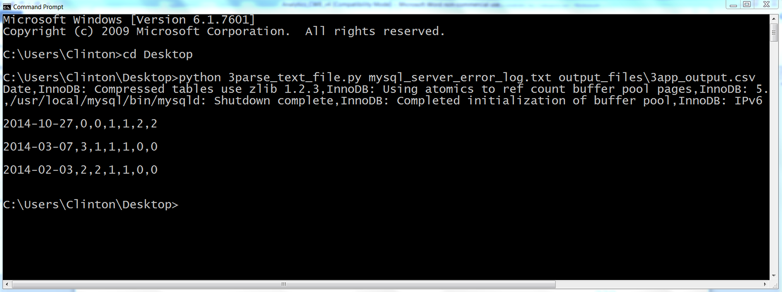
Figure 5-12. The result of running 3parse_text_file.py on the MySQL error log text file, mysql_server_error_log.txt, in a Command Prompt window

The output printed to the Command Prompt window shows the data that has also been written to the output file, 3app.output.csv. The first row of output is the header row, which shows the column headings for all of the columns in the output file. The first column heading, Date, shows that the first column contains the unique dates with error messages recorded in the input file. This column shows that the input file contained three unique dates. The remaining six column headings are the unique error messages that appeared in the input file; therefore, the input file contained six unique error messages. These six columns contain the counts of the number of times each particular error message appeared on each of the dates in the input file. For example, the final column of output shows that the error message InnoDB: IPv6 is available. appeared twice on 2014-10-27, zero times on 2014-02-03, and zero times on 2014-03-07.

The contents of 3app_output.csv, which reflect the output printed to the Command Prompt window, should look as shown in Figure 5-13.

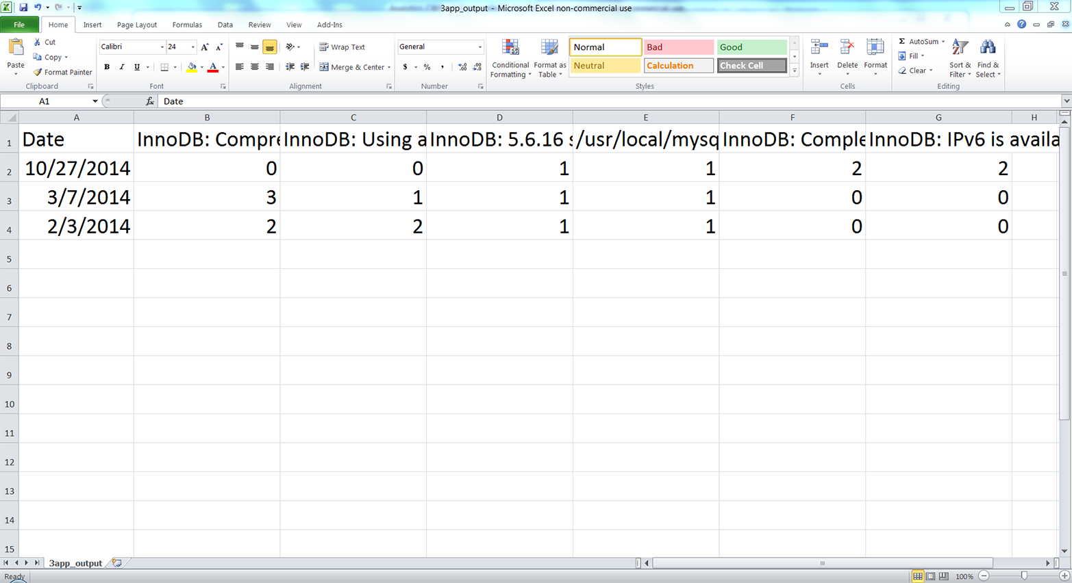
Figure 5-13. The output of 3parse_text_file.py (i.e., the number of times a specific error message occurred on a particular date) in a CSV file named 3app_output.csv, displayed in an Excel worksheet

This screenshot of the CSV output file opened in Excel shows the data written in the output file. The six error messages appear in the header row after the Date heading, although you can’t see the complete messages in this screenshot because of horizontal space constraints (if you create this file, you can expand the columns to read the complete messages).

You will notice that the rows are for specific dates and the columns are for specific error messages. In this small example, there are more unique error messages (i.e., columns) than there are unique dates (i.e., rows). However, in larger log files, there are likely to be more unique dates than unique error messages. In that case, it makes sense to use the (more numerous) rows for specific dates and the columns for specific error messages. Ultimately, whether dates are in rows and error messages are in columns or vice versa depends on your analysis and preferences. A useful exercise for learning would be to modify the existing code to transpose the output, making the dates the columns and the error messages the rows.

This application combined several of the techniques we learned in Chapter 1, like populating a nested dictionary, to tackle a common, real-world problem. Business analysts often run into the problem of needing to parse text files for key pieces of data and aggregate or summarize the data for insights. In many cases, there are thousands or millions of rows that may need to be parsed in different ways, so it would be impossible to parse the rows manually.

In this section, we demonstrated a scalable way to parse data from rows in a text file and calculate basic statistics based on the parsed data. To keep the setup to a minimum, the example only used one short error log file. However, the method scales well, so you can use it to parse larger log files or modify the code to process data from multiple input text files.

Chapter Exercises

1. The first application searches through input files that are saved in one specific folder. However, sometimes input files are saved in several nested folders. Modify the code in the first application so the script will traverse a set of nested folders and process the input files saved in all of the folders. Hint: search for “python os walk” on the Internet.²

2. Modify the second application to calculate the amount of revenue you have earned from customers in the Bronze, Silver, and Gold packages, if the Bronze package is $20/month, the Silver package is $40/month, and the Gold package is $50/month.

3. Practice using dictionaries to bin or group data into unique categories. For example, parse data from an Excel worksheet or a CSV file into a dictionary such that each column in the input file is a key-value pair in the dictionary. That is, each column heading is a key in the dictionary, and the list of values associated with each key are the data values in the associated column.