For Aisha and Amaya,
“Education is the kindling of a flame,
not the filling of a vessel.” —Socrates
May you always enjoy stoking the fire.
Copyright © 2016 Clinton Brownley. All rights reserved.
Printed in the United States of America.
Published by O’Reilly Media, Inc., 1005 Gravenstein Highway North, Sebastopol, CA 95472.
O’Reilly books may be purchased for educational, business, or sales promotional use. Online editions are also available for most titles (http://oreilly.com/safari). For more information, contact our corporate/institutional sales department: 800-998-9938 or corporate@oreilly.com.
See http://oreilly.com/catalog/errata.csp?isbn=9781491922538 for release details.
The O’Reilly logo is a registered trademark of O’Reilly Media, Inc. Foundations for Analytics with Python, the cover image, and related trade dress are trademarks of O’Reilly Media, Inc.
While the publisher and the author have used good faith efforts to ensure that the information and instructions contained in this work are accurate, the publisher and the author disclaim all responsibility for errors or omissions, including without limitation responsibility for damages resulting from the use of or reliance on this work. Use of the information and instructions contained in this work is at your own risk. If any code samples or other technology this work contains or describes is subject to open source licenses or the intellectual property rights of others, it is your responsibility to ensure that your use thereof complies with such licenses and/or rights.
978-1-491-92253-8
[LSI]
This book is intended for readers who deal with data in spreadsheets on a regular basis, but who have never written a line of code. The opening chapters will get you set up with the Python environment, and teach you how to get the computer to look at data and take simple actions with it. Soon, you’ll learn to do things with data in spreadsheets (CSV files) and databases.
At first this will feel like a step backward, especially if you’re a power user of Excel. Painstakingly telling Python how to loop through every cell in a column when you used to select and paste feels slow and frustrating (especially when you have to go back three times to find a typo). But as you become more proficient, you’ll start to see where Python really shines, especially in automating tasks that you currently do over and over.
This book is written so that you can work through it from beginning to end and feel confident that you can write code that works and does what you expect at the end. It’s probably a good idea to type out the code at first, so that you get accustomed to things like tabs and closing your parentheses and quotes, but all the code is available online and you may wind up referring to those links to copy and paste as you do your own work in the future. That’s fine! Knowing when to cut and paste is part of being an efficient programmer. Reading the book as you go through the examples will teach you why and how the code samples work.
Good luck on your journey to becoming a programmer!
If you deal with data on a regular basis, then there are a lot of reasons for you to be excited about learning how to program. One benefit is that you can scale your data processing and analysis tasks beyond what would be feasible or practical to do manually. Perhaps you’ve already come across the problem of needing to process large files that contain so much data that it’s impossible or impractical to open them. Even if you can open the files, processing them manually is time consuming and error prone, because any modifications you make to the data take a long time to update—and with so much data, it’s easy to miss a row or column that you intended to change. Or perhaps you’ve come across the problem of needing to process a large number of files—so many files that it’s impossible or impractical to process them manually. In some cases, you need to use data from dozens, hundreds, or even thousands of files. As the number of files increases, it becomes increasingly difficult to handle them manually. In both of these situations, writing a Python script to process the files solves your problem because Python scripts can process large files and lots of files quickly and efficiently.
Another benefit of learning to program is that you can automate repetitive data manipulation and analysis processes. In many cases, the operations we carry out on data are repetitive and time consuming. For example, a common data management process involves receiving data from a customer or supplier, extracting the data you want to retain, possibly transforming or reformatting the data, and then saving the data in a database or other data repository (this is the process known to data scientists as ETL—extract, transform, load). Similarly, a typical data analysis process involves acquiring the data you want to analyze, preparing the data for analysis, analyzing the data, and reporting the results. In both of these situations, once the process is established, it’s possible to write Python code to carry out the operations. By creating a Python script to carry out the operations, you reduce a time-consuming, repetitive process down to the running of a script and free up your time to work on other impactful tasks.
On top of that, carrying out data processing and analysis operations in a Python script instead of manually reduces the chance of errors. When you process data manually, it’s always possible to make a copy/paste error or a typo. There are lots of reasons why this might happen—you might be working so quickly that you miss the mistake, or you might be distracted or tired. Furthermore, the chance of errors increases when you’re processing large files or lots of files, or when you’re carrying out repetitive actions. Conversely, a Python script doesn’t get distracted or tired. Once you debug your script and confirm that it processes the data the way you want it to, it will carry out the operations consistently and tirelessly.
Finally, learning to program is fun and empowering. Once you’re familiar with the basic syntax, it’s fun to try to figure out which pieces of syntax you need and how to fit them together to accomplish your overall data analysis goal. When it comes to code and syntax, there are lots of examples online that show you how to use specific pieces of syntax to carry out particular tasks. Online examples give you something to work with, but then you need to use your creativity and problem-solving skills to figure out how you need to modify the code you found online to suit your needs. The whole process of searching for the right code and figuring out how to make it work for you can be a lot of fun. Moreover, learning to program is incredibly empowering. For example, consider the situations I mentioned before, involving large files or lots of files. When you can’t program, these situations are either incredibly time consuming or simply infeasible. Once you can program, you can tackle both situations relatively quickly and easily with Python scripts. Being able to carry out data processing and analysis tasks that were once laborious or impossible provides a tremendous rush of positive energy, so much so that you’ll be looking for more opportunities to tackle challenging data processing tasks with Python.
This book is written for people who deal with data on a regular basis and have little to no programming experience. The examples in this book cover common data sources and formats, including text files, comma-separated values (CSV) files, Excel files, and databases. In some cases, these files contain so much data or there are so many files that it’s impractical or impossible to open them or deal with them manually. In other cases, the process used to extract and use the data in the files is time consuming and error prone. In these situations, without the ability to program, you have to spend a lot of your time searching for the data you need, opening and closing files, and copying and pasting data.
Because you may never have run a script before, we’ll start from the very beginning, exploring how to write code in a text file to create a Python script. We’ll then review how to run our Python scripts in a Command Prompt window (for Windows users) and a Terminal window (for macOS users). (If you’ve done a bit of programming, you can skim Chapter 1 and move right into the data analysis parts in Chapter 2.)
Another way I’ve set out to make this book very user-friendly for new programmers is that instead of presenting code snippets that you’d need to figure out how to combine to carry out useful work, the examples in this book contain all of the Python code you need to accomplish a specific task. You might find that you’re coming back to this book as a reference later on, and having all the code at hand will be really helpful then. Finally, following the adage “a picture is worth a thousand words,” this book uses screenshots of the input files, Python scripts, Command Prompt and Terminal windows, and output files so you can literally see how to create the inputs, code, commands, and outputs.
I’m going to go into detail to show how things work, as well as giving you some tools that you can put to use. This approach will help you build a solid basis for understanding “what’s going on under the hood”—there will be times when you Google a solution to your problem and find useful code, and having done the exercises in this book, you’ll have a good understanding of how code you find online works. This means you’ll know both how to apply it in your situation and how to fix it if it breaks. As you’ll build working code through these chapters, you may find that you’ll use this book as a reference, or a “cookbook,” with recipes to accomplish specific tasks. But remember, this is a “learn to cook” book; you’ll be developing skills that you can generalize and combine to do all sorts of tasks.
The majority of examples in this book show how to create and run Python scripts on Microsoft Windows. The focus on Windows is fairly straightforward: I want this book to help as many people as possible, and according to available estimates, the vast majority of desktop and laptop computers—especially in business analytics—run a Windows operating system. For instance, according to Net Applications, as of December 2014, Microsoft Windows occupies approximately 90% of the desktop and laptop operating system market. Because I want this book to appeal to desktop and laptop users, and the vast majority of these computers have a Windows operating system, I concentrate on showing how to create and run Python scripts on Windows.
Despite the book’s emphasis on Windows, I also provide examples of how to create and run Python scripts on macOS, where appropriate. Almost everything that happens within Python itself will happen the same way no matter what kind of machine you’re running it on. But where there are differences between operating systems, I’ll give specific instructions for each. For instance, the first example in Chapter 1 illustrates how to create and run a Python script on both Microsoft Windows and macOS. Similarly, the first examples in Chapters 2 and 3 also illustrate how to create and run the scripts on both Windows and macOS. In addition, Chapter 8 covers both operating systems by showing how to create scheduled tasks on Windows and cron jobs on macOS. If you are a Mac user, use the first example in each chapter as a template for how to create a Python script, make it executable, and run the script. Then repeat the steps to create and run all of the remaining examples in each chapter.
There are many reasons to choose Python if your aim is to learn how to program in a language that will enable you to scale and automate data processing and analysis tasks. One notable feature of Python is its use of whitespace and indentation to denote line endings and blocks of code, in contrast to many other languages, which use extra characters like semicolons and curly braces for these purposes. This makes it relatively easy to see at first glance how a Python program is put together.
The extra characters found in other languages are troublesome for people who are new to programming, for at least two reasons. First, they make the learning curve longer and steeper. When you’re learning to program, you’re essentially learning a new language, and these extra characters are one more aspect of the language you need to learn before you can use the language effectively. Second, they can make the code difficult to read. Because in these other languages semicolons and curly braces denote blocks of code, people don’t always use indentation to guide your eye around the blocks of code. Without indentation, these blocks of code can look like a jumbled mess.
Python sidesteps these difficulties by using whitespace and indentation, not semicolons and curly braces, to denote blocks of code. As you look through Python code, your eyes focus on the actual lines of code rather than the delimiters between blocks of code, because everything around the code is whitespace. Python code requires blocks of code to be indented, and indentation makes it easy to see where one block of code ends and another begins. Moreover, the Python community emphasizes code readability, so there is a culture of writing code that is comparatively easy to read and understand. All of these features make the learning curve shorter and shallower, which means you can get up and running and processing data with Python relatively quickly compared to many alternatives.
Another notable feature of Python that makes it ideal for data processing and analysis is the number of standard and add-in modules and functions that facilitate common data processing and analysis operations. Built-ins and standard library modules and functions come standard with Python, so when you download and install Python you immediately have access to these built-in modules and functions. You can read about all of the built-ins and standard modules in the Python Standard Library (PSL). Add-ins are other Python modules that you download and install separately so you can use the additional functions they provide. You can peruse many of the add-ins in the Python Package Index (PyPI).
Some of the modules in the standard library provide functions for reading different file types (e.g., text, comma-separated values, JSON, HTML, XML, etc.); manipulating numbers, strings, and dates; using regular expression pattern matching; parsing comma-separated values files; calculating basic statistics; and writing data to different output file types and to disk. There are too many useful add-in modules to cover them all, but a few that we’ll use or discuss in this book include the following:
xlrd and xlwtmysqlclient/MySQL-python/MySQLdbpandasstatsmodelsscikit-learnIf you’re new to programming and you’re looking for a programming language that will enable you to automate and scale your data processing and analysis tasks, then Python is an ideal choice. Python’s emphasis on whitespace and indentation means the code is easier to read and understand, which makes the learning curve less steep than for other languages. And Python’s built-in and add-in packages facilitate many common data manipulation and analysis operations, which makes it easy to complete all of your data processing and analysis tasks in one place.
Pandas is an add-in module for Python that provides numerous functions for reading/writing, combining, transforming, and managing data. It also has functions for calculating statistics and creating graphs and plots. All of these functions simplify and reduce the amount of code you need to write to accomplish your data processing tasks. The module has become very popular among data analysts and others who use Python because it offers a lot of helpful functions, it’s fast and powerful, and it simplifies and reduces the code you have to write to get your job done. Given its power and popularity, I want to introduce you to pandas in this book. To do so, I present pandas versions of the scripts in Chapters 2 and 3, I illustrate how to create graphs and plots with pandas in Chapter 6, and I demonstrate how to calculate various statistics with pandas in Chapter 7. I also encourage you to pick up a copy of Wes McKinney’s book, Python for Data Analysis (O’Reilly).1
At the same time, if you’re new to programming, I also want you to learn basic programming skills. Once you learn these skills, you’ll develop generally applicable problem-solving skills that will enable you to break down complex problems into smaller components, solve the smaller components, and then combine the components together to solve the larger problem. You’ll also develop intuition for which data structures and algorithms you can use to solve different problems efficiently and effectively. In addition, there will be times when an add-in module like pandas doesn’t have the functionality you need or isn’t working the way you need it to. In these situations, if you don’t have basic programming skills, you’re stuck. Conversely, if you do have these skills you can create the functionality you need and solve the problem on your own. Being able to solve a programming problem on your own is exhilarating and incredibly empowering.
Because this book is for people who are new to programming, the focus is on basic, generally applicable programming skills. For instance, Chapter 1 introduces fundamental concepts such as data types, data containers, control flow, functions, if-else logic, and reading and writing files. In addition, Chapters 2 and 3 present two versions of each script: a base Python version and a pandas version. In each case, I present and discuss the base Python version first so you learn how to implement a solution on your own with general code, and then I present the pandas version. My hope is that you will develop fundamental programming skills from the base Python versions so you can use the pandas versions with a firm understanding of the concepts and operations pandas simplifies for you.
When it comes to Python, there are a variety of applications in which you can write your code. For example, if you download Python from Python.org, then your installation of Python comes with a graphical user interface (GUI) text editor called Idle. Alternatively, you can download IPython Notebook and write your code in an interactive, web-based environment. If you’re working on macOS or you’ve installed Cygwin on Windows, then you can write your code in a Terminal window using one of the built-in text editors like Nano, Vim, or Emacs. If you’re already familiar with one of these applications, then feel free to use it to follow along with the examples in this book.
However, in this section, I’m going to provide instructions for downloading and installing the free Anaconda Python distribution from Continuum Analytics because it has some advantages over the alternatives for a beginning programmer—and for the advanced programmer, too! The major advantage is that it comes with hundreds of the most popular add-in Python packages preinstalled so you don’t have to experience the inevitable headaches of trying to install them and their dependencies on your own. For example, all of the add-in packages we use in this book come preinstalled in Anaconda Python.
Another advantage is that it comes with an integrated development environment, or IDE, called Spyder. Spyder provides a convenient interface for writing, executing, and debugging your code, as well as installing packages and launching IPython Notebooks. It includes nice features such as links to online documentation, syntax coloring, keyboard shortcuts, and error warnings.
Another nice aspect of Anaconda Python is that it’s cross-platform—there are versions for Linux, Mac, and Windows. So if you learn to use it on Windows but need to transition to a Mac at a later point, you’ll still be able to use the same familiar interface.
One aspect of Anaconda Python to keep in mind while you’re becoming familiar with Python and all of the available add-in packages is the syntax you use to install add-in packages. In Anaconda Python, you use the conda install command. For example, to install the add-in package argparse, you would type conda install argparse. This syntax is different from the usual pip install command you’d use if you’d installed Python from Python.org (if you’d installed Python from Python.org, then you’d install the argparse package with python -m pip install argparse). Anaconda Python also allows you to use the pip install syntax, so you can actually use either method, but it’s helpful to be aware of this slight difference while you’re learning to install add-in packages.
To install Anaconda Python, follow these steps:
Go to http://continuum.io/downloads (the website automatically detects your operating system—i.e., Windows or Mac).
Select “Windows 64-bit Python 3.5 Graphical Installer” (if you’re using Windows) or “Mac OS X 64-bit Python 3.5 Graphical Installer” (if you’re on a Mac).
Double-click the downloaded .exe (for Windows) or .pkg (for Mac) file.
Follow the installer’s instructions.
Although we’ll be using Anaconda Python and Spyder in this book, it’s helpful to be familiar with some text editors that provide features for writing Python code. For instance, if you didn’t want to use Anaconda Python, you could simply install Python from Python.org and then use a text editor like Notepad (for Windows) or TextEdit (for macOS). To use TextEdit to write Python scripts, you need to open TextEdit and change the radio button under TextEdit→Preferences from “Rich text” to “Plain text” so new files open as plain text. Then you’ll be able to save the files with a .py extension.
An advantage of writing your code in a text editor is that there should already be one on your computer, so you don’t have to worry about downloading and installing additional software. And as most desktops and laptops ship with a text editor, if you ever have to work on a different computer (e.g., one that doesn’t have Spyder or a Terminal window), you’ll be able to get up and running quickly with whatever text editor is available on the computer.
While writing your Python code in a text editor such as Notepad or TextEdit is completely acceptable and effective, there are other free text editors you can download that offer additional features, including code highlighting, adjustable tab sizes, and multi-line indenting and dedenting. These features (particularly code highlighting and multi-line indenting and dedenting) are incredibly helpful, especially while you’re learning to write and debug your code.
Here is a noncomprehensive list of some free text editors that offer these features:
Notepad++ (Windows)
Sublime Text (Windows and Mac)
jEdit (Windows and Mac)
TextWrangler (Mac)
Again, I’ll be using Anaconda Python and Spyder in this book, but feel free to use a text editor to follow along with the examples. If you download one of these editors, be sure to search online for the keystroke combination to use to indent and dedent multiple lines at a time. It’ll make your life a lot easier when you start experimenting with and debugging blocks of code.
All of the Python scripts, input files, and output files presented in this book are available online at https://github.com/cbrownley/foundations-for-analytics-with-python.
It’s possible to download the whole folder of materials to your computer, but it’s probably simpler to just click on the filename and copy/paste the script into your text editor. (GitHub is a website for sharing and collaborating on code—it’s very good at keeping track of different versions of a project and managing the collaboration process, but it has a pretty steep learning curve. When you’re ready to start sharing your code and suggesting changes to other people’s code, you might take a look at Chad Thompson’s Learning Git (Infinite Skills).)
We’ll begin by exploring how to create and run a Python script. This chapter focuses on basic Python syntax and the elements of Python that you need to know for later chapters in the book. For example, we’ll discuss basic data types such as numbers and strings and how you can manipulate them. We’ll also cover the main data containers (i.e., lists, tuples, and dictionaries) and how you use them to store and manipulate your data, as well as how to deal with dates, as dates often appear in business analysis. This chapter also discusses programming concepts such as control flow, functions, and exceptions, as these are important elements for including business logic in your code and gracefully handling errors. Finally, the chapter explains how to get your computer to read a text file, read multiple text files, and write to a CSV-formatted output file. These are important techniques for accessing input data and retaining specific output data that I expand on in later chapters in the book.
This chapter covers how to read and write CSV files. The chapter starts with an example of parsing a CSV input file “by hand,” without Python’s built-in csv module. It transitions to an illustration of potential problems with this method of parsing and then presents an example of how to avoid these potential problems by parsing a CSV file with Python’s csv module. Next, the chapter discusses how to use three different types of conditional logic to filter for specific rows from the input file and write them to a CSV output file. Then the chapter presents two different ways to filter for specific columns and write them to the output file. After covering how to read and parse a single CSV input file, we’ll move on to discussing how to read and process multiple CSV files. The examples in this section include presenting summary information about each of the input files, concatenating data from the input files, and calculating basic statistics for each of the input files. The chapter ends with a couple of examples of less common procedures, including selecting a set of contiguous rows and adding a header row to the dataset.
Next, we’ll cover how to read Excel workbooks with a downloadable, add-in module called xlrd. This chapter starts with an example of introspecting an Excel workbook (i.e., presenting how many worksheets the workbook contains, the names of the worksheets, and the number of rows and columns in each of the worksheets). Because Excel stores dates as numbers, the next section illustrates how to use a set of functions to format dates so they appear as dates instead of as numbers. Next, the chapter discusses how to use three different types of conditional logic to filter for specific rows from a single worksheet and write them to a CSV output file. Then the chapter presents two different ways to filter for specific columns and write them to the output file. After covering how to read and parse a single worksheet, the chapter moves on to discuss how to read and process all worksheets in a workbook and a subset of worksheets in a workbook. The examples in these sections show how to filter for specific rows and columns in the worksheets. After discussing how to read and parse any number of worksheets in a single workbook, the chapter moves on to review how to read and process multiple workbooks. The examples in this section include presenting summary information about each of the workbooks, concatenating data from the workbooks, and calculating basic statistics for each of the workbooks. The chapter ends with a couple of examples of less common procedures, including selecting a set of contiguous rows and adding a header row to the dataset.
Here, we’ll cover how to carry out basic database operations in Python. The chapter starts with examples that use Python’s built-in sqlite3 module so that you don’t have to install any additional software. The examples illustrate how to carry out some of the most common database operations, including creating a database and table, loading data in a CSV input file into a database table, updating records in a table using a CSV input file, and querying a table. When you use the sqlite3 module, the database connection details are slightly different from the ones you would use to connect to other database systems like MySQL, PostgreSQL, and Oracle. To show this difference, the second half of the chapter demonstrates how to interact with a MySQL database system. If you don’t already have MySQL on your computer, the first step is to download and install MySQL. From there, the examples mirror the sqlite3 examples, including creating a database and table, loading data in a CSV input file into a database table, updating records in a table using a CSV input file, querying a table, and writing query results to a CSV output file. Together, the examples in the two halves of this chapter provide a solid foundation for carrying out common database operations in Python.
This chapter contains three examples that demonstrate how to combine techniques presented in earlier chapters to tackle three different problems that are representative of some common data processing and analysis tasks. The first application covers how to find specific records in a large collection of Excel and CSV files. As you can imagine, it’s a lot more efficient and fun to have a computer search for the records you need than it is to search for them yourself. Opening, searching in, and closing dozens of files isn’t fun, and the task becomes more and more challenging as the number of files increases. Because the problem involves searching through CSV and Excel files, this example utilizes a lot of the material covered in Chapters 2 and 3.
The second application covers how to group or “bin” data into unique categories and calculate statistics for each of the categories. The specific example is parsing a CSV file of customer service package purchases that shows when customers paid for particular service packages (i.e., Bronze, Silver, or Gold), organizing the data into unique customer names and packages, and adding up the amount of time each customer spent in each package. The example uses two building blocks, creating a function and storing data in a dictionary, which are introduced in Chapter 1 but aren’t used in Chapters 2, 3, and 4. It also introduces another new technique: keeping track of the previous row you processed and the row you’re currently processing, in order to calculate a statistic based on values in the two rows. These two techniques—grouping or binning data with a dictionary and keeping track of the current row and the previous row—are very powerful capabilities that enable you to handle many common analysis tasks that involve events over time.
The third application covers how to parse a text file, group or bin data into categories, and calculate statistics for the categories. The specific example is parsing a MySQL error log file, organizing the data into unique dates and error messages, and counting the number of times each error message appeared on each date. The example reviews how to parse a text file, a technique that briefly appears in Chapter 1. The example also shows how to store information separately in both a list and a dictionary in order to create the header row and the data rows for the output file. This is a reminder that you can parse text files with basic string operations and another good example of how to use a nested dictionary to group or bin data into unique categories.
In this chapter, you’ll learn how to create common statistical graphs and plots in Python with four plotting libraries: matplotlib, pandas, ggplot, and seaborn. The chapter begins with matplotlib because it’s a long-standing package with lots of documentation (in fact, pandas and seaborn are built on top of matplotlib). The matplotlib section illustrates how to create histograms and bar, line, scatter, and box plots. The pandas section discusses some of the ways pandas simplifies the syntax you need to create these plots and illustrates how to create them with pandas. The ggplot section notes the library’s historical relationship with R and the Grammar of Graphics and illustrates how to use ggplot to build some common statistical plots. Finally, the seaborn section discusses how to create standard statistical plots as well as plots that would be more cumbersome to code in matplotlib.
Here, we’ll look at how to produce standard summary statistics and estimate regression and classification models with the pandas and statsmodels packages. pandas has functions for calculating measures of central tendency (e.g., mean, median, and mode), as well as for calculating dispersion (e.g., variance and standard deviation). It also has functions for grouping data, which makes it easy to calculate these statistics for different groups of data. The statsmodels package has functions for estimating many types of regression and classification models. The chapter illustrates how to build multivariate linear regression and logistic classification models based on data in pandas DataFrames and then use the models to predict output values for new input data.
This chapter covers how to schedule your scripts to run automatically on a routine basis on both Windows and macOS. Until this chapter, we ran the scripts manually on the command line. Running a script manually on the command line is convenient when you’re debugging the script or running it on an ad hoc basis. However, it can be a nuisance if your script needs to run on a routine basis (e.g., daily, weekly, monthly, or quarterly), or if you need to run lots of scripts on a routine basis. On Windows, you create scheduled tasks to run scripts automatically on a routine basis. On macOS, you create cron jobs, which perform the same actions. This chapter includes several screenshots to show you how to create and run scheduled tasks and cron jobs. By scheduling your scripts to run on a routine basis, you don’t ever forget to run a script and you can scale beyond what’s possible when you’re running scripts manually on the command line.
The final chapter covers some additional built-in and add-in Python modules and functions that are important for data processing and analysis tasks, as well as some additional data structures that will enable you to efficiently handle a variety of complex programming problems you may run into as you move beyond the topics covered in this book. Built-ins are bundled into the Python installation, so they are immediately available to you when you install Python. The built-in modules discussed in this chapter include collections, random, statistics, itertools, and operator. The built-in functions include enumerate, filter, reduce, and zip. Add-in modules don’t come with the Python installation, so you have to download and install them separately. The add-in modules discussed in this chapter include NumPy, SciPy, and Scikit-Learn. We also take a look at some additional data structures that can help you store, process, or analyze your data more quickly and efficiently, such as stacks, queues, trees, and graphs.
The following typographical conventions are used in this book:
Indicates new terms, URLs, email addresses, filenames, and file extensions.
Constant widthUsed for program listings, as well as within paragraphs to refer to program elements such as variable or function names, databases, data types, environment variables, statements, and keywords. Also used for module and package names, and to show commands or other text that should be typed literally by the user and the output of commands.
Constant width italicShows text that should be replaced with user-supplied values or by values determined by context.
This element signifies a tip or suggestion.
This element signifies a general note.
This element signifies a warning or caution.
Supplemental material (virtual machine, data, scripts, and custom command-line tools, etc.) is available for download at https://github.com/cbrownley/foundations-for-analytics-with-python.
This book is here to help you get your job done. In general, if example code is offered with this book, you may use it in your programs and documentation. You do not need to contact us for permission unless you’re reproducing a significant portion of the code. For example, writing a program that uses several chunks of code from this book does not require permission. Selling or distributing a CD-ROM of examples from O’Reilly books does require permission. Answering a question by citing this book and quoting example code does not require permission. Incorporating a significant amount of example code from this book into your product’s documentation does require permission.
We appreciate, but do not require, attribution. An attribution usually includes the title, author, publisher, and ISBN. For example: “Foundations for Analytics with Python by Clinton Brownley (O’Reilly). Copyright 2016 Clinton Brownley, 978-1-491-92253-8.”
If you feel your use of code examples falls outside fair use or the permission given above, feel free to contact us at permissions@oreilly.com.
Safari (formerly Safari Books Online) is a membership-based training and reference platform for enterprise, government, educators, and individuals.
Members have access to thousands of books, training videos, Learning Paths, interactive tutorials, and curated playlists from over 250 publishers, including O’Reilly Media, Harvard Business Review, Prentice Hall Professional, Addison-Wesley Professional, Microsoft Press, Sams, Que, Peachpit Press, Adobe, Focal Press, Cisco Press, John Wiley & Sons, Syngress, Morgan Kaufmann, IBM Redbooks, Packt, Adobe Press, FT Press, Apress, Manning, New Riders, McGraw-Hill, Jones & Bartlett, and Course Technology, among others.
For more information, please visit http://oreilly.com/safari.
Please address comments and questions concerning this book to the publisher:
To comment or ask technical questions about this book, send email to bookquestions@oreilly.com.
For more information about our books, courses, conferences, and news, see our website at http://www.oreilly.com.
Find us on Facebook: http://facebook.com/oreilly
Follow us on Twitter: http://twitter.com/oreillymedia
Watch us on YouTube: http://www.youtube.com/oreillymedia
Follow Clinton on Twitter: @ClintonBrownley
I wrote this book to help people with no or little programming experience, people not unlike myself a few years ago, learn some fundamental programming skills so they can feel the exhilaration of being able to tackle data processing and analysis projects that previously would have been prohibitively time consuming or impossible.
I wouldn’t have been able to write this book without the training, guidance, and support of many people. First and foremost, I would like to thank my wife, Anushka, who spent countless hours teaching me fundamental programming concepts. She helped me learn how to break down large programming tasks into smaller tasks and organize them with pseudocode; how to use lists, dictionaries, and conditional logic effectively; and how to write generalized, scalable code. At the beginning, she kept me focused on solving the programming task instead of worrying about whether my code was elegant or efficient. Then, after I’d become more proficient, she was always willing to review a script and suggest ways to improve it. Once I started writing the book, she provided similar support. She reviewed all of the scripts and suggested ways to make them shorter, clearer, and more efficient. She also reviewed a lot of the text and suggested where I should add to, chop, or alter the text to make the instructions and explanations easier to read and understand. As if all of this training and advice wasn’t enough, Anushka also provided tremendous assistance and support during the months I spent writing. She took care of our daughters during the nights and weekends I was away writing, and she provided encouragement in the moments when the writing task seemed daunting. This book wouldn’t have been possible without all of the instruction, guidance, critique, support, and love she’s provided over the years.
I’d also like to thank my friends and colleagues at work who encouraged, supported, and contributed to my programming training. Heather Marquez and Ashish Kelkar were incredibly supportive. They helped me attend training courses and work on projects that enhanced and broadened my programming skills. Later, when I informed them I’d created a set of training materials and wanted to teach a 10 day training course, they helped make it a successful experience. Rajiv Krishnamurthy also contributed to my education. Over the period of a few weeks, he posed a variety of programming problems for me to solve and met with me each week to discuss, critique, and improve my solutions. Vikram Rao reviewed the linear and logistic regression sections and provided helpful suggestions on ways to clarify key points about the regression models. I’d also like to thank many of my other colleagues, who, either for a project or simply to help me understand a concept or technique, shared their code with me, reviewed my code and suggested improvements, or pointed me to informative resources.
I’d also like to thank three Python training instructors, Marilyn Davis, Jeremy Osborne, and Jonathan Rocher. Marilyn and Jeremy’s courses covered fundamental programming concepts and how to implement them in Python. Jonathan’s course covered the scientific Python stack, including numpy, scipy, matplotlib and seaborn, pandas, and scikit-learn. I thoroughly enjoyed their courses, and each one enriched and expanded my understanding of fundamental programming concepts and how to implement them in Python.
I’d also like to thank the people at O’Reilly Media who have contributed to this book. Timothy McGovern was a jovial companion through the writing and editing process. He reviewed each of the drafts and offered insightful suggestions on the collection of topics to include in the book and the amount of content to include in each chapter. He also suggested ways to change the text, layout, and format in specific sections to make them easier to read and understand. I’d like to thank his colleagues, Marie Beaugureau and Rita Scordamalgia, for escorting me into the O’Reilly publishing process and providing marketing resources. I’d also like to thank Colleen Cole and Jasmine Kwityn for superbly editing all of the chapters and producing the book. Finally, I’d like to thank Ted Kwartler for reviewing the first draft of the manuscript and providing helpful suggestions for improving the book. His review encouraged me to include the visualization and statistical analysis chapters, to accompany each of the base Python scripts with pandas versions, and to remove some of the text and examples to reduce repetition and improve readability. The book is richer and more well-rounded because of his thoughtful suggestions.
1 Wes McKinney is the original developer of the pandas module and his book is an excellent introduction to pandas, NumPy, and IPython (additional add-in modules you’ll want to learn about as you broaden your knowledge of Python for data analysis).
Many books and online tutorials about Python show you how to execute code in the Python shell. To run Python code in this way, you’ll open a Command Prompt window (in Windows) or a Terminal window (in macOS) and type “python” to get a Python prompt (which looks like >>>). Then simply type your commands one at a time; Python will execute them.
Here are two typical examples:
>>> 4 + 5
9

>>> print("I'm excited to learn Python.")
I'm excited to learn Python.
This method of executing code is fast and fun, but it doesn’t scale well as the number of lines of code grows. When what you want to accomplish requires many lines of code, it is easier to write all of the code in a text file as a Python script, and then run the script. The following section shows you how to create a Python script.
Open the Spyder IDE or a text editor (e.g., Notepad, Notepad++, or Sublime Text on Windows; TextMate, TextWrangler, or Sublime Text on macOS).
Write the following two lines of code in the text file:
#!/usr/bin/env python3("Output #1: I'm excited to learn Python.")
The first line is a special line called the shebang, which you should always include as the very first line in your Python scripts. Notice that the first character is the pound or hash character (#). The # precedes a single-line comment, so the line of code isn’t read or executed on a Windows computer. However, Unix computers use the line to find the version of Python to use to execute the code in the file. Because Windows machines ignore this line and Unix-based systems such as macOS use it, including the line makes the script transferable among the different types of computers.
The second line is a simple print statement. This line will print the text between the double quotes to the Command Prompt (Windows) or a Terminal window (macOS).
Open the Save As dialog box.
In the location box, navigate to your Desktop so the file will be saved on your Desktop.
In the format box, select All Files so that the dialog box doesn’t select a file type.
In the Save As box or File Name box, type “first_script.py”. In the past, you’ve probably saved a text file as a .txt file. However, in this case you want to save it as a .py file to create a Python script.
Click Save.
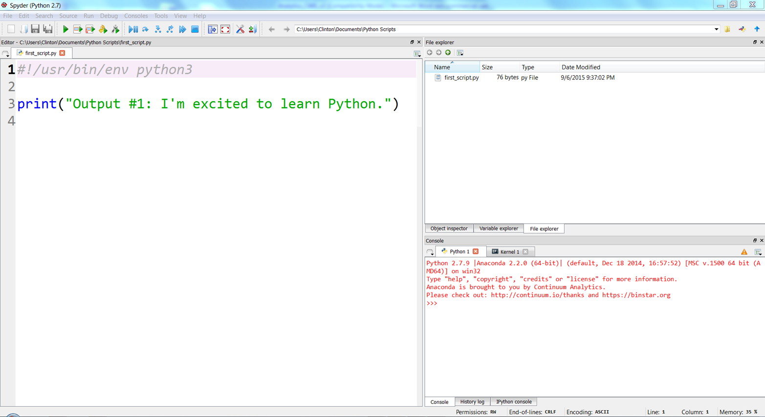
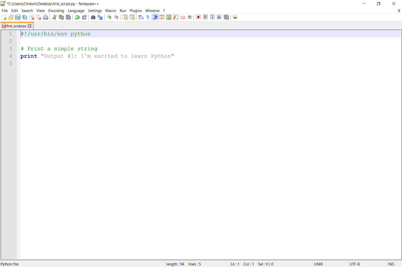
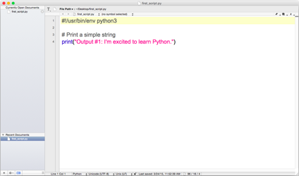
You’ve now created a Python script. Figures 1-1, 1-2, and 1-3 show what it looks like in Anaconda Spyder, Notepad++ (Windows), and TextWrangler (macOS), respectively.
The next section will explain how to run the Python script in the Command Prompt or Terminal window. You’ll see that it’s as easy to run it as it was to create it.
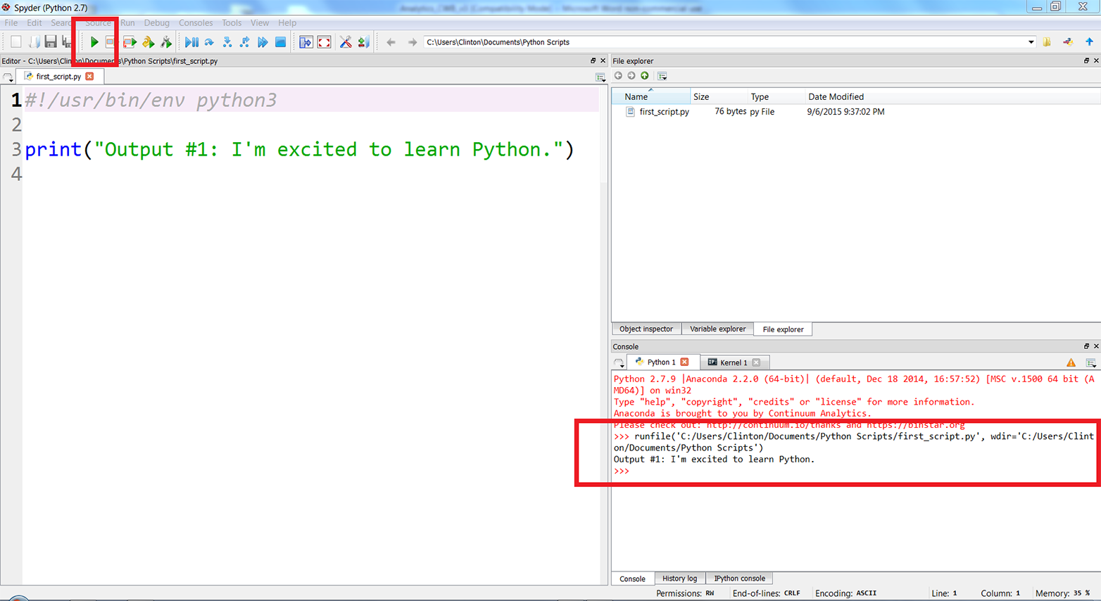
If you created the file in the Anaconda Spyder IDE, you can run the script by clicking on the green triangle (the Run button) in the upper-lefthand corner of the IDE.
When you click the Run button, you’ll see the output displayed in the Python console in the lower-righthand pane of the IDE. The screenshot displays both the green run button and the output inside red boxes (see Figure 1-4). In this case, the output is “Output #1: I’m excited to learn Python.”
Alternatively, you can run the script in a Command Prompt (Windows) or Terminal window (macOS), as described next:
Open a Command Prompt window.
When the window opens the prompt will be in a particular folder, also known as a directory (e.g., C:\Users\Clinton or C:\Users\Clinton\Documents).
Navigate to the Desktop (where we saved the Python script).
To do so, type the following line and then hit Enter:
cd "C:\Users\[Your Name]\Desktop"
Replace [Your Name] with your computer account name, which is usually your name. For example, on my computer, I’d type:
cd "C:\Users\Clinton\Desktop"
At this point, the prompt should look like C:\Users\[Your Name]\Desktop, and we are exactly where we need to be, as this is where we saved the Python script. The last step is to run the script.
Run the Python script.
To do so, type the following line and then hit Enter:
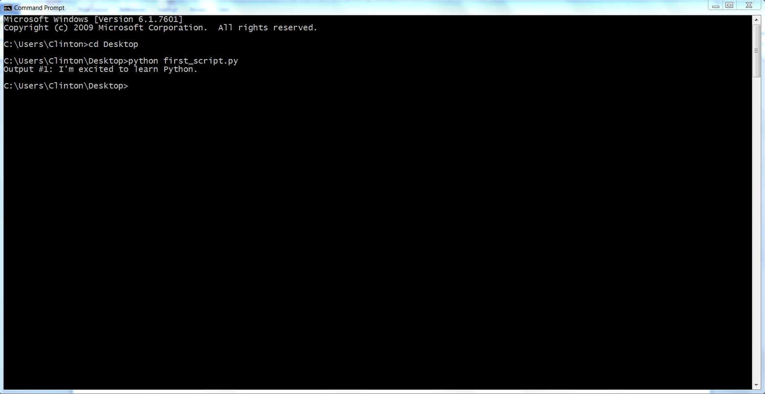
python first_script.pyYou should see the following output printed to the Command Prompt window, as in Figure 1-5:
Output #1: I'm excited to learn Python.
Open a Terminal window.
When the window opens, the prompt will be in a particular folder, also known as a directory (e.g., /Users/clinton or /Users/clinton/Documents).
Navigate to the Desktop, where we saved the Python script.
To do so, type the following line and then hit Enter:
cd /Users/[Your Name]/Desktop
Replace [Your Name] with your computer account name, which is usually your name. For example, on my computer I’d type:
cd /Users/clinton/Desktop
At this point, the prompt should look like /Users/[Your Name]/Desktop, and we are exactly where we need to be, as this is where we saved the Python script. The next steps are to make the script executable and then to run the script.
Make the Python script executable.
To do so, type the following line and then hit Enter:
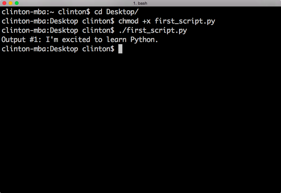
chmod +x first_script.py
The chmod command is a Unix command that stands for change access mode. The +x specifies that you are adding the execute access mode, as opposed to the read or write access modes, to your access settings so Python can execute the code in the script. You have to run the chmod command once for each Python script you create to make the script executable. Once you’ve run the chmod command on a file, you can run the script as many times as you like without retyping the chmod command.
Run the Python script.
To do so, type the following line and then hit Enter:
./first_script.py
You should see the following output printed to the Terminal window, as in Figure 1-6:
Output #1: I'm excited to learn Python.
Here are some useful tips for interacting with the command line:
One nice feature of Command Prompt and Terminal windows is that you can press the up arrow to retrieve your previous command. Try pressing the up arrow in your Command Prompt or Terminal window now to retrieve your previous command, python first_script.py on Windows or ./first_script.py on Mac.
This feature, which reduces the amount of typing you have to do each time you want to run a Python script, is very convenient, especially when the name of the Python script is long or you’re supplying additional arguments (like the names of input files or output files) on the command line.
Now that you’ve run a Python script, this is a good time to mention how to interrupt and stop a Python script. There are quite a few situations in which it behooves you to know how to stop a script. For example, it’s possible to write code that loops endlessly, such that your script will never finish running. In other cases, you may write a script that takes a long time to complete and decide that you want to halt the script prematurely if you’ve included print statements and they show that it’s not going to produce the desired output.
To interrupt and stop a script at any point after you’ve started running it, press Ctrl+c (on Windows) or Control+c (on macOS). This will stop the process that you started with your command. You won’t need to worry too much about the technical details, but a process is a computer’s way of looking at a sequence of commands. You write a script or program and the computer interprets it as a process, or, if it’s more complicated, as a series of processes that may go on sequentially or at the same time.
While we’re on the topic of dealing with troublesome scripts, let’s also briefly talk about what to do when you type ./python first_script.py, or attempt to run any Python script, and instead of running it properly your Command Prompt or Terminal window shows you an error message. The first thing to do is relax and read the error message. In some cases, the error message clearly directs you to the line in your code with the error so you can focus your efforts around that line to debug the error (your text editor or IDE will have a setting to show you line numbers; if it doesn’t do it automatically, poke around in the menus or do a quick search on the Web to figure out how to do this). It’s also important to realize that error messages are a part of programming, so learning to code involves learning how to debug errors effectively.
Moreover, because error messages are common, it’s usually relatively easy to figure out how to debug an error. You’re probably not the first person to have encountered the error and looked for solutions online—one of your best options is to copy the entire error message, or at least the generic portion of the message, into your search engine (e.g., Google or Bing) and look through the results to read about how other people have debugged the error.
It’s also helpful to be familiar with Python’s built-in exceptions, so you can recognize these standard error messages and know how to fix the errors. You can read about Python’s built-in exceptions in the Python Standard Library, but it’s still helpful to search for these error messages online to read about how other people have dealt with them.
Now, to become more comfortable with writing Python code and running your Python script, try editing first_script.py by adding more lines of code and then rerunning the script. For extended practice, add each of the blocks of code shown in this chapter at the bottom of the script beneath any preceding code, resave the script, and then rerun the script.
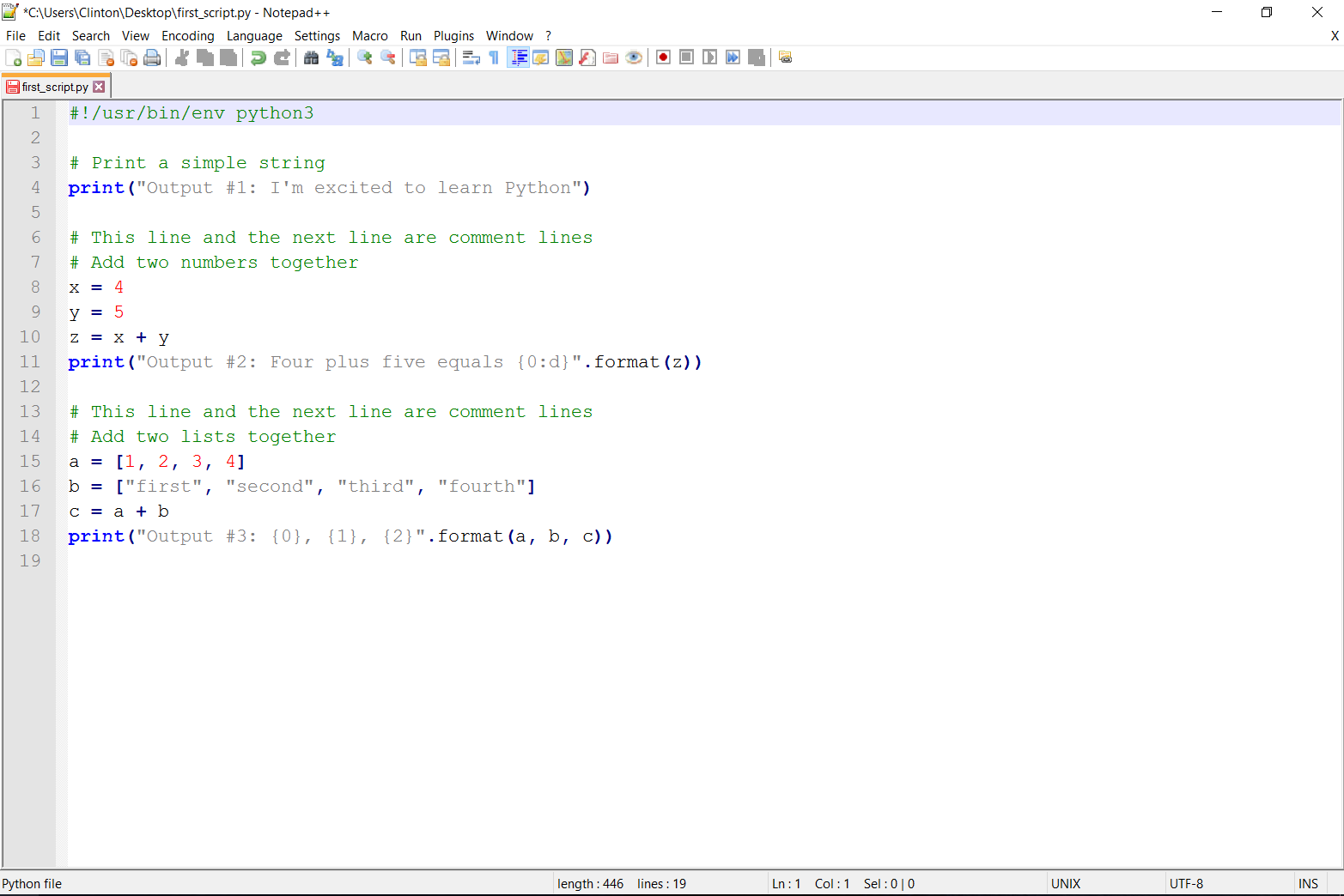
For example, add the two blocks of code shown here below the existing print statement, then resave and rerun the script (remember, after you add the lines of code to first_script.py and resave the script, if you’re using a Command Prompt or Terminal window, you can press the up arrow to retrieve the command you use to run the script so you don’t have to type it again):
# Add two numbers togetherx=4y=5z=x+y("Output #2: Four plus five equals {0:d}.".format(z))# Add two lists togethera=[1,2,3,4]b=["first","second","third","fourth"]c=a+b("Output #3: {0}, {1}, {2}".format(a,b,c))
The lines that are preceded by a # are comments, which can be used to annotate the code and describe what it’s intended to do.
The first of these two examples shows how to assign numbers to variables, add variables together, and format a print statement. Let’s examine the syntax in the print statement, "{0:d}".format(z). The curly braces ({}) are a placeholder for the value that’s going to be passed into the print statement, which in this case comes from the variable z. The 0 points to the first position in the variable z. In this case, z contains a single value, so the 0 points to that value; however, if z were a list or tuple and contained many values, the 0 would specify to only pull in the first value from z.
The colon (:) separates the value to be pulled in from the formatting of that value. The d specifies that the value should be formatted as a digit with no decimal places. In the next section, you’ll learn how to specify the number of decimal places to show for a floating-point number.
The second example shows how to create lists, add lists together, and print variables separated by commas to the screen. The syntax in the print statement, "{0}, {1}, {2}".format(a, b, c), shows how to include multiple values in the print statement. The value a is passed into {0}, the value b is passed into {1}, and the value c is passed into {2}. Because all three of these values are lists, as opposed to numbers, we don’t specify a number format for the values. We’ll discuss these procedures and many more in later sections of this chapter.
Figure 1-7 and Figure 1-8 show what it looks like to add the new code in Anaconda Spyder and in Notepad++.
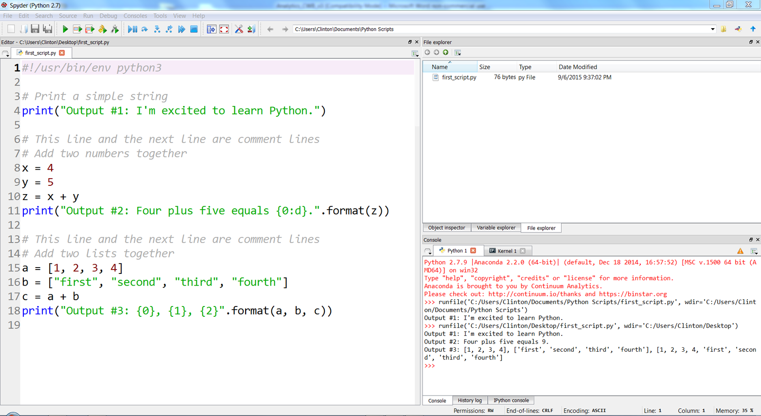
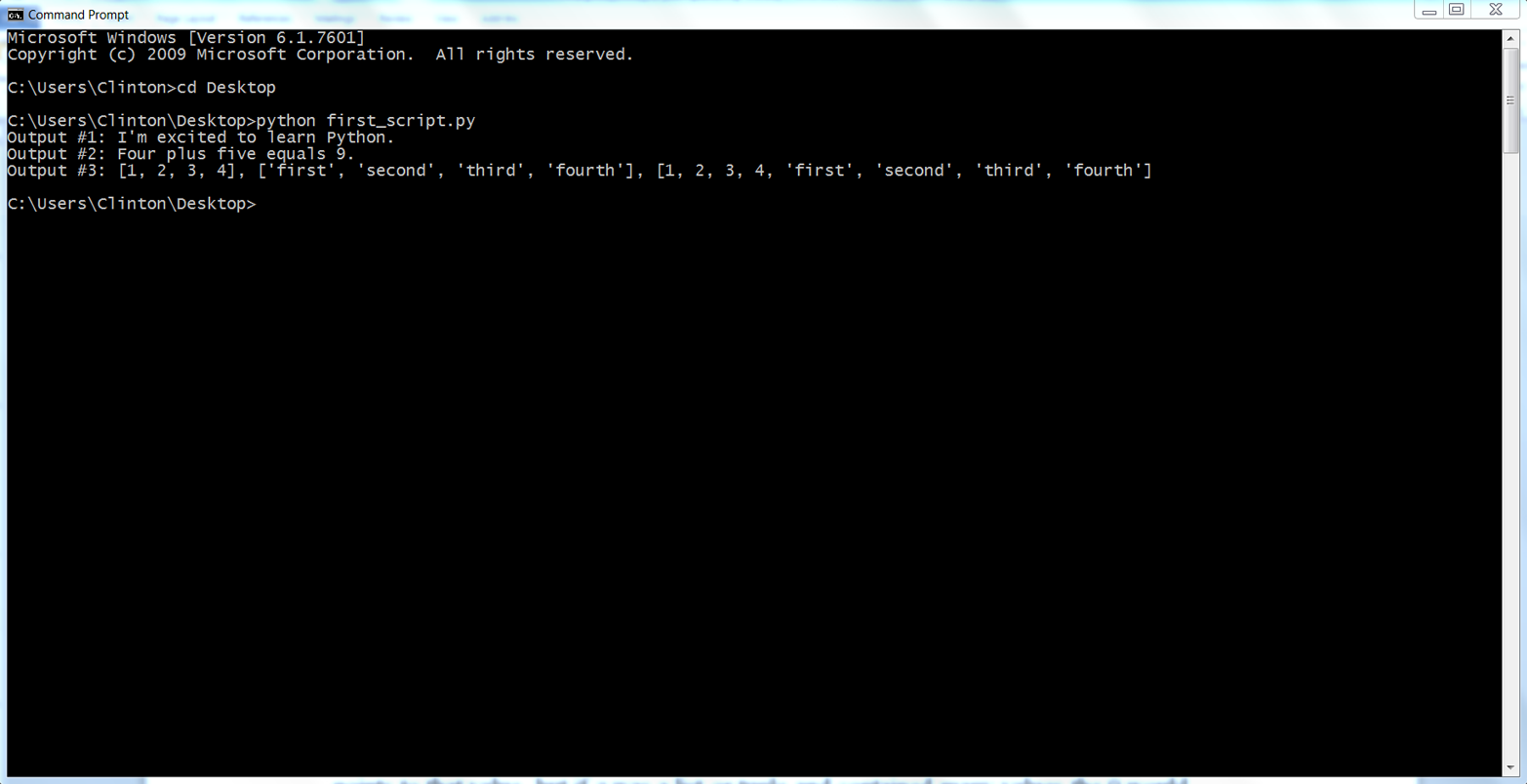
If you add the preceding lines of code to first_script.py, then when you resave and rerun the script you should see the following output printed to the screen (see Figure 1-9:
Output #1: I'm excited to learn Python.
Output #2: Four plus five equals 9.
Output #3: [1, 2, 3, 4], ['first', 'second', 'third', 'fourth'],
[1, 2, 3, 4, 'first', 'second', 'third', 'fourth']
Now that you can create and run Python scripts, you have the basic skills necessary for writing Python scripts that can automate and scale existing manual business processes. Later chapters will go into much more detail about how to use Python scripts to automate and scale these processes, but before moving on it’s important to become more familiar with some of Python’s basic building blocks. By becoming more familiar with these building blocks, you’ll understand and be much more comfortable with how they’ve been combined in later chapters to accomplish specific data processing tasks. First, we’ll deal with some of the most common data types in Python, and then we’ll work through ways to make your programs make decisions about data with if statements and functions. Next, we’ll work with the practicalities of having Python read and write to files that you can use in other programs or read directly: text and simple table (CSV) files.
Python has several built-in numeric types. This is obviously great, as many business applications require analyzing and processing numbers. The four main types of numbers in Python are integer, floating-point, long, and complex numbers. We’ll cover integer and floating-point numbers, as they are the most common in business applications. You can add the following examples dealing with integer and floating-point numbers to first_script.py, beneath the existing examples, and rerun the script to see the output printed to the screen.
Let’s dive straight into a few examples involving integers:
x=9("Output #4: {0}".format(x))("Output #5: {0}".format(3**4))("Output #6: {0}".format(int(8.3)/int(2.7)))
Output #4 shows how to assign an integer, the number 9, to the variable x and how to print the x variable. Output #5 illustrates how to raise the number 3 to the power of 4 (which equals 81) and print the result. Output #6 demonstrates how to cast numbers as integers and perform division. The numbers are cast as integers with the built-in int function, so the equation becomes 8 divided by 2, which equals 4.0.
Like integers, floating-point numbers—numbers with decimal points—are very important to many business applications. The following are a few examples involving floating-point numbers:
("Output #7: {0:.3f}".format(8.3/2.7))y=2.5*4.8("Output #8: {0:.1f}".format(y))r=8/float(3)("Output #9: {0:.2f}".format(r))("Output #10: {0:.4f}".format(8.0/3))
Output #7 is much like Output #6, except we’re keeping the numbers to divide as floating-point numbers, so the equation is 8.3 divided by 2.7: approximately 3.074. The syntax in the print statement in this example, "{0:.3f}".format(floating_point_number/floating_point_number), shows how to specify the number of decimal places to show in the print statement. In this case, the .3f specifies that the output value should be printed with three decimal places.
Output #8 shows multiplying 2.5 times 4.8, assigning the result into the variable y, and printing the value with one decimal place. Multiplying these two floating-point numbers together results in 12, so the value printed is 12.0. Outputs #9 and #10 show dividing the number 8 by the number 3 in two different ways. The result in both, approximately 2.667, is a floating-point number.
An important detail to know about dealing with numbers in Python is that there are several standard library modules and built-in functions and modules you can use to perform common mathematical operations. You’ve already seen two built-in functions, int and float, for manipulating numbers. Another useful standard module is the math module.
Python’s standard modules are on your computer when you install Python, but when you start up a new script, the computer only loads a very basic set of operations (this is part of why Python is quick to start up). To make a function in the math module available to you, all you have to do is add from math import [function name] at the top of your script, right beneath the shebang. For example, add the following line at the top of first_script.py, below the shebang:
#!/usr/bin/env python3frommathimportexp,log,sqrt
Once you’ve added this line to the top of first_script.py, you have three useful mathematical functions at your disposal. The functions exp, log, and sqrt take the number e to the power of the number in parentheses, the natural log of the number in parentheses, and the square root of the number in parentheses, respectively. The following are a few examples of using these math module functions:
("Output #11: {0:.4f}".format(exp(3)))("Output #12: {0:.2f}".format(log(4)))("Output #13: {0:.1f}".format(sqrt(81)))
The results of these three mathematical expressions are floating-point numbers, approximately 20.0855, 1.39, and 9.0, respectively.
This is just the beginning of what’s available in the math module. There are many more useful mathematical functions and modules built into Python, for business, scientific, statistical, and other applications, and we’ll discuss quite a few more in this book. For more information about these and other standard modules and built-in functions, you can peruse the Python Standard Library.
A string is another basic data type in Python; it usually means human-readable text, and that’s a useful way to think about it, but it is more generally a sequence of characters that only has meaning when they’re all in that sequence. Strings appear in many business applications, including supplier and customer names and addresses, comment and feedback data, event logs, and documentation. Some things look like integers, but they’re actually strings. Think of zip codes, for example. The zip code 01111 (Springfield, Massachusetts) isn’t the same as the integer 1111—you can’t (meaningfully) add, subtract, multiply, or divide zip codes—and you’d do well to treat zip codes as strings in your code. This section covers some modules, functions, and operations you can use to manage strings.
Strings are delimited by single, double, triple single, or triple double quotation marks. The following are a few examples of strings:
("Output #14: {0:s}".format('I\'m enjoying learning Python.'))("Output #15: {0:s}".format("This is a long string. Without the backslash\itwouldrunoffofthepageontherightinthetexteditorandbevery\difficulttoreadandedit.Byusingthebackslashyoucansplitthelong\stringintosmallerstringsonseparatelinessothatthewholestringiseasy\toviewinthetexteditor."))("Output #16: {0:s}".format('''You can use triple single quotesfor multi-line comment strings.'''))("Output #17: {0:s}".format("""You can also use triple double quotesfor multi-line comment strings."""))
Output #14 is similar to the one at the beginning of this chapter. It shows a simple string delimited by single quotes. The result of this print statement is "I'm enjoying learning Python.". Remember, if we had used double quotes to delimit the string it wouldn’t have been necessary to include a backslash before the single quote in the contraction "I'm".
Output #15 shows how you can use a single backslash to split a long one-line string across multiple lines so that it’s easier to read and edit. Although the string is split across multiple lines in the script, it is still a single string and will print as a single string. An important point about this method of splitting a long string across multiple lines is that the backslash must be the last character on the line. This means that if you accidentally hit the spacebar so that there is an invisible space after the backslash, your script will throw a syntax error instead of doing what you want it to do. For this reason, it’s prudent to use triple single or triple double quotes to create multi-line strings.
Outputs #16 and #17 show how to use triple single and triple double quotes to create multi-line strings. The output of these examples is:
Output #16: You can use triple single quotes
for multi-line comment strings.
Output #17: You can also use triple double quotes
for multi-line comment strings.
When you use triple single or double quotes, you do not need to include a backslash at the end of the top line. Also, notice the difference between Output #15 and Outputs #16 and #17 when printed to the screen. The code for Output #15 is split across multiple lines with single backslashes as line endings, making each line of code shorter and easier to read, but it prints to the screen as one long line of text. Conversely, Outputs #16 and #17 use triple single and double quotes to create multi-line strings and they print to the screen on separate lines.
As with numbers, there are many standard modules, built-in functions, and operators you can use to manage strings. A few useful operators and functions include +, *, and len. The following are a few examples of using these operators on strings:
string1="This is a "string2="short string."sentence=string1+string2("Output #18: {0:s}".format(sentence))("Output #19: {0:s} {1:s}{2:s}".format("She is","very "*4,"beautiful."))m=len(sentence)("Output #20: {0:d}".format(m))
Output #18 shows how to add two strings together with the + operator. The result of this print statement is This is a short string—the + operator adds the strings together exactly as they are, so if you want spaces in the resulting string, you have to add spaces in the smaller string segments (e.g., after the letter “a” in Output #18) or between the string segments (e.g., after the word “very” in Output #19).
Output #19 shows how to use the * operator to repeat a string a specific number of times. In this case, the resulting string contains four copies of the string “very ” (i.e., the word “very” followed by a single space).
Output #20 shows how to use the built-in len function to determine the number of characters in the string. The len function also counts spaces and punctuation in the string’s length. Therefore, the string This is a short string. in Output #20 is 23 characters long.
A useful standard library module for dealing with strings is the string module. With the string module, you have access to many functions that are useful for managing strings. The following sections discuss a few examples of using these string functions.
The following two examples show how to use the split function to break a string into a list of the substrings that make up the original string. (The list is another built-in data type in Python that we’ll discuss later in this chapter.) The split function can take up to two additional arguments between the parentheses. The first additional argument indicates the character(s) on which the split should occur. The second additional argument indicates how many splits to perform (e.g., two splits results in three substrings):
string1="My deliverable is due in May"string1_list1=string1.split()string1_list2=string1.split(" ",2)("Output #21: {0}".format(string1_list1))("Output #22: FIRST PIECE:{0} SECOND PIECE:{1} THIRD PIECE:{2}"\.format(string1_list2[0],string1_list2[1],string1_list2[2]))string2="Your,deliverable,is,due,in,June"string2_list=string2.split(',')("Output #23: {0}".format(string2_list))("Output #24: {0} {1} {2}".format(string2_list[1],string2_list[5],\string2_list[-1]))
In Output #21, there are no additional arguments between the parentheses, so the split function splits the string on the space character (the default). Because there are five spaces in this string, the string is split into a list of six substrings. The newly created list is ['My', 'deliverable', 'is', 'due', 'in', 'May'].
In Output #22, we explicitly include both arguments in the split function. The first argument is " ", which indicates that we want to split the string on a single space character. The second argument is 2, which indicates that we only want to split on the first two single space characters. Because we specify two splits, we create a list with three elements. The second argument can come in handy when you’re parsing data. For example, you may be parsing a log file that contains a timestamp, an error code, and an error message separated by spaces. In this case, you may want to split on the first two spaces to parse out the timestamp and error code, but not split on any remaining spaces so the error message remains intact.
In Outputs #23 and #24, the additional argument between the parentheses is a comma. In this case, the split function splits the string wherever there is a comma. The resulting list is ['Your', 'deliverable', 'is', 'due', 'in', 'June'].
The next example shows how to use the join function to combine substrings contained in a list into a single string. The join function takes an argument before the word join, which indicates the character(s) to use between the substrings as they are combined:
("Output #25: {0}".format(','.join(string2_list)))
In this example, the additional argument—a comma—is included between the parentheses. Therefore, the join function combines the substrings into a single string with commas between the substrings. Because there are six substrings in the list, the substrings are combined into a single string with five commas between the substrings. The newly created string is Your,deliverable,is,due,in,June.
The next two sets of examples show how to use the strip, lstrip, and rstrip functions to remove unwanted characters from the ends of a string. All three functions can take an additional argument between the parentheses to specify the character(s) to be removed from the ends of the string.
The first set of examples shows how to use the lstrip, rstrip, and strip functions to remove spaces, tabs, and newline characters from the lefthand side, righthand side, and both sides of the string, respectively:
string3=" Remove unwanted characters from this string.\t\t\n"("Output #26: string3: {0:s}".format(string3))string3_lstrip=string3.lstrip()("Output #27: lstrip: {0:s}".format(string3_lstrip))string3_rstrip=string3.rstrip()("Output #28: rstrip: {0:s}".format(string3_rstrip))string3_strip=string3.strip()("Output #29: strip: {0:s}".format(string3_strip))
The lefthand side of string3 contains several spaces. In addition, on the righthand side, there are tabs (\t), more spaces, and a newline (\n) character. If you haven’t seen the \t and \n characters before, they are the way a computer represents tabs and newlines.
In Output #26, you’ll see leading whitespace before the sentence; you’ll see a blank line below the sentence as a result of the newline character, and you won’t see the tabs and spaces after the sentence, but they are there. Outputs #27, #28, and #29 show you how to remove the spaces, tabs, and newline characters from the lefthand side, righthand side, and both sides of the string, respectively. The s in {0:s} indicates that the value passed into the print statement should be formatted as a string.
This second set of examples shows how to remove other characters from the ends of a string by including them as the additional argument in the strip function.
string4="$$Here's another string that has unwanted characters.__---++"("Output #30: {0:s}".format(string4))string4="$$The unwanted characters have been removed.__---++"string4_strip=string4.strip('$_-+')("Output #31: {0:s}".format(string4_strip))
In this case, the dollar sign ($), underscore (_), dash (-), and plus sign (+) need to be removed from the ends of the string. By including these characters as the additional argument, we tell the program to remove them from the ends of the string. The resulting string in Output #31 is The unwanted characters have been removed..
The next two examples show how to use the replace function to replace one character or set of characters in a string with another character or set of characters. The function takes two additional arguments between the parentheses—the first argument is the character or set of characters to find in the string and the second argument is the character or set of characters that should replace the characters in the first argument:
string5="Let's replace the spaces in this sentence with other characters."string5_replace=string5.replace(" ","!@!")("Output #32 (with !@!): {0:s}".format(string5_replace))string5_replace=string5.replace(" ",",")("Output #33 (with commas): {0:s}".format(string5_replace))
Output #32 shows how to use the replace function to replace the single spaces in the string with the characters !@!. The resulting string is Let's!@!replace!@!the!@!spaces !@!in!@!this!@!sentence!@!with!@!other!@!characters..
Output #33 shows how to replace single spaces in the string with commas. The resulting string is Let's,replace,the,spaces,in,this,sentence,with,other,characters..
The final three examples show how to use the lower, upper, and capitalize functions. The lower and upper functions convert all of the characters in the string to lowercase and uppercase, respectively. The capitalize function applies upper to the first character in the string and lower to the remaining characters:
string6="Here's WHAT Happens WHEN You Use lower."("Output #34: {0:s}".format(string6.lower()))string7="Here's what Happens when You Use UPPER."("Output #35: {0:s}".format(string7.upper()))string5="here's WHAT Happens WHEN you use Capitalize."("Output #36: {0:s}".format(string5.capitalize()))string5_list=string5.split()("Output #37 (on each word):")forwordinstring5_list:("{0:s}".format(word.capitalize()))
Outputs #34 and #35 are straightforward applications of the lower and upper functions. After applying the functions to the strings, all of the characters in string6 are lowercase and all of the characters in string7 are uppercase.
Outputs #36 and #37 demonstrate the capitalize function. Output #36 shows that the capitalize function applies upper to the first character in the string and lower to the remaining characters. Output #37 places the capitalize function in a for loop. A for loop is a control flow structure that we’ll discuss later in this chapter, but let’s take a sneak peak.
The phrase for word in string5_list: basically says, “For each element in the list, string5_list, do something.” The next phrase, print word.capitalize(), is what to do to each element in the list. Together, the two lines of code basically say, “For each element in the list, string5_list, apply the capitalize function to the element and print the element.” The result is that the first character of each word in the list is capitalized and the remaining characters of each word are lowercased.
There are many more modules and functions for managing strings in Python. As with the built-in math functions, you can peruse the Python Standard Library for more about them.
Many business analyses rely on pattern matching, also known as regular expressions. For example, you may need to perform an analysis on all orders from a specific state (e.g., where state is Maryland). In this case, the pattern you’re looking for is the word Maryland. Similarly, you may want to analyze the quality of a product from a specific supplier (e.g., where the supplier is StaplesRUs). Here, the pattern you’re looking for is StaplesRUs.
Python includes the re module, which provides great functionality for searching for specific patterns (i.e., regular expressions) in text. To make all of the functionality provided by the re module available to you in your script, add import re at the top of the script, right beneath the previous import statement. Now the top of first_script.py should look like:
#!/usr/bin/env python3frommathimportexp,log,sqrtimportre
By importing the re module, you gain access to a wide variety of metacharacters and functions for creating and searching for arbitrarily complex patterns. Metacharacters are characters in the regular expression that have special meaning. In their unique ways, metacharacters enable the regular expression to match several different specific strings. Some of the most common metacharacters are |, ( ), [ ], ., *, +, ?, ^, $, and (?P<name>). If you see these characters in a regular expression, you’ll know that the software won’t be searching for these characters in particular but something they describe. You can read more about these metacharacters in the “Regular Expression Operations” section of the Python Standard Library.
The re module also contains several useful functions for creating and searching for specific patterns (the functions covered in this section are re.compile, re.search, re.sub, and re.ignorecase or re.I). Let’s take a look at the example:
# Count the number of times a pattern appears in a stringstring="The quick brown fox jumps over the lazy dog."string_list=string.split()pattern=re.compile(r"The",re.I)count=0forwordinstring_list:ifpattern.search(word):count+=1("Output #38: {0:d}".format(count))
The first line assigns the string The quick brown fox jumps over the lazy dog. to the variable string. The next line splits the string into a list with each word, a string, as an element in the list.
The next line uses the re.compile and re.I functions, and the raw string r notation, to create a regular expression called regexp. The re.compile function compiles the text-based pattern into a compiled regular expression. It isn’t always necessary to compile the regular expression, but it is good practice because doing so can significantly increase a program’s speed. The re.I function ensures that the pattern is case-insensitive and will match both “The” and “the” in the string. The raw string notation, r, ensures Python will not process special sequences in the string, such as \, \t, or \n. This means there won’t be any unexpected interactions between string special sequences and regular expression special sequences in the pattern search. There are no string special sequences in this example, so the r isn’t necessary in this case, but it is good practice to use raw string notation in regular expressions. The next line creates a variable named count to hold the number of times the pattern appears in the string and sets its initial value to 0.
The next line is a for loop that will iterate over each of the elements in the list variable string_list. The first element it grabs is the word “The”, the second element it grabs is the word “quick”, and so on and so forth through each of the words in the list.
The next line uses the re.search function to compare each word in the list to the regular expression. The function returns True if the word matches the regular expression and returns None or False otherwise. So the if statement says, “If the word matches the regular expression, add 1 to the value in count.”
Finally, the print statement prints the number of times the regular expression found the pattern “The”, case-insensitive, in the string—in this case, two times.
Regular expressions are very powerful when searching, but they’re a bear for people to read (they’ve been called a “write-only language”), so don’t worry if it’s hard for you to understand one on first reading; even the experts have difficulty with this!
As you get more comfortable with regular expressions, it can even become a bit of a game to get them to produce the results you want. For a fun trip through this topic, you can see Google Director of Research Peter Norvig’s attempt to create a regexp that will match US presidents’ names—and reject losing candidates for president—at https://www.oreilly.com/learning/regex-golf-with-peter-norvig.
Let’s look at another example:
# Print the pattern each time it is found in the stringstring="The quick brown fox jumps over the lazy dog."string_list=string.split()pattern=re.compile(r"(?P<match_word>The)",re.I)("Output #39:")forwordinstring_list:ifpattern.search(word):("{:s}".format(pattern.search(word).group('match_word')))
This second example is different from the first example in that we want to print each matched string to the screen instead of simply counting the number of matches. To capture the matched strings so they can be printed to the screen or a file, we need to use the (?P<name>) metacharacter and the group function. Most of the code in this example is identical to the code discussed in the first example, so I’ll focus on the new parts.
The first new piece of code snippet, (?P<name>), is a metacharacter that appears inside the re.compile function. This metacharacter makes the matched string available later in the program through the symbolic group name <name>. In this example, I called the group <match_word>.
The final new code snippet appears in the if statement. This code snippet basically says, “If the result evaluates to True (i.e., if the word matches the pattern), then look in the data structure returned by the search function and grab the value in the group called match_word, and print the value to the screen.”
Here’s one last example:
# Substitute the letter "a" for the word "the" in the stringstring="The quick brown fox jumps over the lazy dog."string_to_find=r"The"pattern=re.compile(string_to_find,re.I)("Output #40: {:s}".format(pattern.sub("a",string)))
This final example shows how to use the re.sub function to substitute one pattern for another pattern in text. Once again, most of the code in this example is similar to that in the first two examples, so I’ll just focus on the new parts.
The first new code snippet assigns the regular expression to a variable, pattern, so the variable can be passed into the re.compile function. Assigning the regular expression to a variable before the re.compile function isn’t necessary, as mentioned; however, if you have a long, complex regular expression, assigning it to a variable and then passing the variable to the re.compile function can make your code much more readable.
The final new code snippet appears in the last line. This code snippet uses the re.sub function to look for the pattern, The, case-insensitive, in the variable named string and replace every occurrence of the pattern with the letter a. The result of this substitution is a quick brown fox jumps over a lazy dog.
For more information about other regular expression functions, you can peruse the Python Standard Library or Michael Fitzgerald’s book Introducing Regular Expressions (O’Reilly).
Dates are an essential consideration in most business applications. You may need to know when an event will occur, the amount of time until an event occurs, or the amount of time between events. Because dates are central to so many applications—and because they’re such a downright weird sort of data, working in multiples of sixty, twenty-four, “about thirty,” and “almost exactly three hundred sixty-five and a quarter,” there are special ways of handling dates in Python.
Python includes the datetime module, which provides great functionality for dealing with dates and times. To make all of the functionality provided by the datetime module available to you in your script, add from datetime import date, time, datetime, timedelta at the top of your script beneath the previous import statement. Now the top of first_script.py should look like:
#!/usr/bin/env python3frommathimportexp,log,sqrtimportrefromdatetimeimportdate,time,datetime,timedelta
When you import the datetime module, you have a wide variety of date and time objects and functions at your disposal. Some of the useful objects and functions include today, year, month, day, timedelta, strftime, and strptime. These functions make it possible to capture individual elements of a date (e.g., year, month, or day), to add or subtract specific amounts of time to or from dates, to create date strings with specific formats, and to create datetime objects from date strings. The following are a few examples of how to use these datetime objects and functions. The first set of examples illustrates the difference between a date object and a datetime object:
# Print today's date, as well as the year, month, and day elementstoday=date.today()("Output #41: today: {0!s}".format(today))("Output #42: {0!s}".format(today.year))("Output #43: {0!s}".format(today.month))("Output #44: {0!s}".format(today.day))current_datetime=datetime.today()("Output #45: {0!s}".format(current_datetime))
By using date.today(), you create a date object that includes year, month, and day elements but does not include any of the time elements, like hours, minutes, and seconds. Contrast this with datetime.today(), which does include the time elements. The !s in {0!s} indicates that the value being passed into the print statement should be formatted as a string, even though it’s a number. Finally, you can use year, month, and day to capture these individual date elements.
This next example demonstrates how to use the timedelta function to add or subtract specific amounts of time to or from a date object:
# Calculate a new date using a timedeltaone_day=timedelta(days=-1)yesterday=today+one_day("Output #46: yesterday: {0!s}".format(yesterday))eight_hours=timedelta(hours=-8)("Output #47: {0!s} {1!s}".format(eight_hours.days,eight_hours.seconds))
In this example, we use the timedelta function to subtract one day from today’s date. Alternatively, we could have used days=10, hours=-8, or weeks=2 inside the parentheses to create a variable that is ten days into the future, eight hours into the past, or two weeks into the past, respectively.
One thing to keep in mind when using timedelta is that it stores time differences inside the parentheses as days, seconds, and microseconds and then normalizes the values to make them unique. This means that minutes, hours, and weeks are converted to 60 seconds, 3,600 seconds, and 7 days, respectively, and then normalized, essentially creating days, seconds, and microseconds “columns” (think back to grade-school math and the ones column, tens column, and so on). For example, the output of hours=-8 is (-1 days, 57,600 seconds) rather than the simpler (-28,800 seconds). This is calculated as 86,400 seconds (3,600 seconds per hour * 24 hours per day) – 28,800 seconds (3,600 seconds per hour * 8 hours) = 57,600 seconds. As you can see, the output of normalizing negative values can be surprising initially, especially when truncating and rounding.
The third example shows how to subtract one date object from another. The result of the subtraction is a datetime object that shows the difference in days, hours, minutes, and seconds. For example, in this case the result is “1 day, 0:00:00”:
# Calculate the number of days between two datesdate_diff=today-yesterday("Output #48: {0!s}".format(date_diff))("Output #49: {0!s}".format(str(date_diff).split()[0]))
In some cases, you may only need the numeric element of this result. For instance, in this example you may only need the number 1. One way to grab this number from the result is to use some of the functions you already learned about for manipulating strings. The str function converts the result to a string; the split function splits the string on whitespace and makes each of the substrings an element in a list; and the [0] says “grab the first element in the list,” which in this case is the number 1. We’ll see the [0] syntax again in the next section, which covers lists, because it illustrates list indexing and shows how you can retrieve specific elements from a list.
The fourth set of examples shows how to use the strftime function to create a string with a specific format from a date object:
# Create a string with a specific format from a date object("Output #50: {:s}".format(today.strftime('%m/%d/%Y')))("Output #51: {:s}".format(today.strftime('%b%d,%Y')))("Output #52: {:s}".format(today.strftime('%Y-%m-%d')))("Output #53: {:s}".format(today.strftime('%B%d,%Y')))
At the time of writing this chapter, the four formats print today’s date as:
01/28/2016
Jan 28, 2016
2016-01-28
January 28, 2016
These four examples show how to use some of the formatting symbols, including %Y, %B, %b, %m, and %d, to create different date-string formats. You can see the other formatting symbols the datetime module uses in the “datetime—Basic date and time types” section of the Python Standard Library.
# Create a datetime object with a specific format# from a string representing a datedate1=today.strftime('%m/%d/%Y')date2=today.strftime('%b%d,%Y')date3=today.strftime('%Y-%m-%d')date4=today.strftime('%B%d,%Y')# Two datetime objects and two date objects# based on the four strings that have different date formats("Output #54: {!s}".format(datetime.strptime(date1,'%m/%d/%Y')))("Output #55: {!s}".format(datetime.strptime(date2,'%b%d,%Y')))# Show the date portion only("Output #56: {!s}".format(datetime.date(datetime.strptime\(date3,'%Y-%m-%d'))))("Output #57: {!s}".format(datetime.date(datetime.strptime\(date4,'%B%d,%Y'))))
The fifth set of examples shows how to use the strptime function to create a datetime object from a date string that has a specific format. In this example, date1, date2, date3, and date4 are string variables that show today’s date in different formats: The first two print statements show the result of converting the first two string variables, date1 and date2, into datetime objects. To work correctly, the format used in the strptime function needs to match the format of the string variable being passed into the function. The result of these print statements is a datetime object, 2014-01-28 00:00:00.
Sometimes, you may only be interested in the date portion of the datetime object. In this case, you can use the nested functions, date and strptime, shown in the last two print statements, to convert date-string variables to datetime objects and then return only the date portion of the datetime object. The result of these print statements is 2014-01-28. Of course, you do not need to print the value immediately. You can assign the date to a new variable and then use the variable in calculations to generate insights about your business data over time.
Lists are prevalent in many business analyses. You may have lists of customers, products, assets, sales figures, and on and on. But lists—ordered collections of objects—in Python are even more flexible than that! All those types of lists contain similar objects (e.g., strings containing the names of customers or floating-point numbers representing sales figures), but lists in Python do not have to be that simple. They can contain an arbitrary mix of numbers, strings, other lists, and tuples and dictionaries (described later in this chapter). Because of their prevalence, flexibility, and importance in most business applications, it is critical to know how to manipulate lists in Python.
As you might expect, Python provides many useful functions and operators for managing lists. The following sections demonstrate how to use some of the most common and helpful of these functions and operators.
# Use square brackets to create a list# len() counts the number of elements in a list# max() and min() find the maximum and minimum values# count() counts the number of times a value appears in a lista_list=[1,2,3]("Output #58: {}".format(a_list))("Output #59: a_list has {} elements.".format(len(a_list)))("Output #60: the maximum value in a_list is {}.".format(max(a_list)))("Output #61: the minimum value in a_list is {}.".format(min(a_list)))another_list=['printer',5,['star','circle',9]]("Output #62: {}".format(another_list))("Output #63: another_list also has {} elements.".format\(len(another_list)))("Output #64: 5 is in another_list {} time.".format(another_list.count(5)))
This example shows how to create two simple lists, a_list and another_list. You create a list by placing elements between square brackets. a_list contains the numbers 1, 2, and 3. another_list contains the string printer, the number 5, and a list with two strings and one number.
This example also shows how to use four list functions: len, min, max, and count. len shows the number of elements in a list. min and max show the minimum and the maximum values in a list, respectively. count shows the number of times a specific value appears in the list.
# Use index values to access specific elements in a list# [0] is the first element; [-1] is the last element("Output #65: {}".format(a_list[0]))("Output #66: {}".format(a_list[1]))("Output #67: {}".format(a_list[2]))("Output #68: {}".format(a_list[-1]))("Output #69: {}".format(a_list[-2]))("Output #70: {}".format(a_list[-3]))("Output #71: {}".format(another_list[2]))("Output #72: {}".format(another_list[-1]))
This example shows how you can use list index values, or indices, to access specific elements in a list. List index values start at 0, so you can access the first element in a list by placing a 0 inside square brackets after the name of the list. The first print statement in this example, print a_list[0], prints the first element in a_list, which is the number 1. a_list[1] accesses the second element in the list, a_list[2] accesses the third element, and so on to the end of the list.
This example also shows that you can use negative indices to access elements at the end of a list. Index values at the end of a list start at –1, so you can access the last element in a list by placing –1 inside square brackets after the name of the list. The fourth print statement, print a_list[-1], prints the last element in a_list, which is the number 3. a_list[-2] accesses the second-to-last element in the list, a_list[-3] accesses the third-to-last element in the list, and so on to the beginning of the list.
# Use list slices to access a subset of list elements# Do not include a starting index to start from the beginning# Do not include an ending index to go all of the way to the end("Output #73: {}".format(a_list[0:2]))("Output #74: {}".format(another_list[:2]))("Output #75: {}".format(a_list[1:3]))("Output #76: {}".format(another_list[1:]
This example shows how to use list slices to access a subset of list elements. You create a list slice by placing two indices separated by a colon between square brackets after the name of the list. List slices access list elements from the first index value to the element one place before the second index value. For example, the first print statement, print a_list[0:2], basically says, “Print the elements in a_list whose index values are 0 and 1.” This print statement prints [1, 2], as these are the first two elements in the list.
This example also shows that you do not need to include the first index value if the list slice starts from the beginning of the list, and you do not need to include the second index value if the list slice continues to the end of the list. For example, the last print statement, print another_list[1:], basically says, “Print all of the remaining elements in another_list, starting with the second element.” This print statement prints [5, ['star', 'circle', 9]], as these are the last two elements in the list.
# Use [:] to make a copy of a lista_new_list=a_list[:]("Output #77: {}".format(a_new_list))
This example shows how to make a copy of a list. This capability is important for when you need to manipulate a list in some way, perhaps by adding or removing elements or sorting the list, but you want the original list to remain unchanged. To make a copy of a list, place a single colon inside square brackets after the name of the list and assign it to a new variable. In this example, a_new_list is an exact copy of a_list, so you can add elements or remove them from a_new_list or sort a_new_list without modifying a_list.
# Use + to add two or more lists togethera_longer_list=a_list+another_list("Output #78: {}".format(a_longer_list))
This example shows how to concatenate two or more lists together. This capability is important for when you have to access lists of similar information separately, but you want to combine all of the lists together before analyzing them. For example, because of how your data is stored, you may have to generate one list of sales figures from one data source and another list of sales figures from a different data source. To concatenate the two lists of sales figures together for analysis, add the names of the two lists together with the + operator and assign the sum to a new variable. In this example, a_longer_list contains the elements of a_list and another_list concatenated together into a single, longer list.
# Use in and not in to check whether specific elements are or are not in a lista=2ina_list("Output #79: {}".format(a))if2ina_list:("Output #80: 2 is in {}.".format(a_list))b=6notina_list("Output #81: {}".format(b))if6notina_list:("Output #82: 6 is not in {}.".format(a_list))
This example shows how to use in and not in to check whether specific elements are in a list or not. The results of these expressions are True or False values, depending on whether the expressions are true or false. These capabilities are important for business applications because you can use them to add meaningful business logic to your program. For example, they are often used in if statements such as “if SupplierY in SupplierList then do something, else do something else.” We will see more examples of if statements and other control flow expressions later in this chapter.
# Use append() to add additional elements to the end of the list# Use remove() to remove specific elements from the list# Use pop() to remove elements from the end of the lista_list.append(4)a_list.append(5)a_list.append(6)("Output #83: {}".format(a_list))a_list.remove(5)("Output #84: {}".format(a_list))a_list.pop()a_list.pop()("Output #85: {}".format(a_list))
This example shows how to add elements to and remove elements from a list. The append method adds single elements to the end of a list. You can use this method to create lists according to specific business rules. For example, to create a list of CustomerX’s purchases, you could create an empty list called CustomerX, scan through a master list of all purchases, and when the program “sees” CustomerX in the master list, append the purchase value to the CustomerX list.
The remove method removes a specific value from anywhere in a list. You can use this method to remove errors and typos from a list or to remove values from a list according to specific business rules. In this example, the remove method removes the number 5 from a_list.
The pop method removes single elements from the end of a list. Like with the remove method, you can use the pop method to remove errors and typos from the end of a list or to remove values from the end of a list according to specific business rules. In this example, the two calls to the pop method remove the numbers 6 and 4 from the end of a_list, respectively.
# Use reverse() to reverse a list in-place, meaning it changes the list# To reverse a list without changing the original list, make a copy firsta_list.reverse()("Output #86: {}".format(a_list))a_list.reverse()("Output #87: {}".format(a_list))
This example shows how to use the reverse function to reverse a list in-place. “In-place” means the reversal changes the original list to the new, reversed order. For example, the first call to the reverse function in this example changes a_list to [3, 2, 1]. The second call to the reverse function returns a_list to its original order. To use a reversed copy of a list without modifying the original list, first make a copy of the list and then reverse the copy.
# Use sort() to sort a list in-place, meaning it changes the list# To sort a list without changing the original list, make a copy firstunordered_list=[3,5,1,7,2,8,4,9,0,6]("Output #88: {}".format(unordered_list))list_copy=unordered_list[:]list_copy.sort()("Output #89: {}".format(list_copy))("Output #90: {}".format(unordered_list))
This example shows how to use the sort function to sort a list in-place. As with the reverse method, this in-place sort changes the original list to the new, sorted order. To use a sorted copy of a list without modifying the original list, first make a copy of the list and then sort the copy.
# Use sorted() to sort a collection of lists by a position in the listsmy_lists=[[1,2,3,4],[4,3,2,1],[2,4,1,3]]my_lists_sorted_by_index_3=sorted(my_lists,key=lambdaindex_value:\index_value[3])("Output #91: {}".format(my_lists_sorted_by_index_3))
This example shows how to use the sorted function in combination with a key function to sort a collection of lists by the value in a specific index position in each list. The key function specifies the key to be used to sort the lists. In this case, the key is a lambda function that says, “Sort the lists by the values in index position three (i.e., the fourth values in the lists).” (We’ll talk a bit more about lambda functions later.) After applying the sorted function with the fourth value in each list as the sort key, the second list [4,3,2,1] becomes the first list, the third list [2,4,1,3] becomes the second list, and the first list [1,2,3,4] becomes the third list. Also, note that whereas the sort function sorts the list in-place, changing the order of the original list, the sorted function returns a new sorted list and does not change the order of the original list.
The next sorting example uses the standard operator module, which provides functionality for sorting lists, tuples, and dictionaries by multiple keys. To use the operator module’s itemgetter function in your script, add from operator import itemgetter at the top of your script:
#!/usr/bin/env python3frommathimportexp,log,sqrtimportrefromdatetimeimportdate,time,datetime,timedeltafromoperatorimportitemgetter
By importing the operator module’s itemgetter function, you can sort a collection of lists by multiple positions in each list:
# Use itemgetter() to sort a collection of lists by two index positionsmy_lists=[[123,2,2,444],[22,6,6,444],[354,4,4,678],[236,5,5,678],\[578,1,1,290],[461,1,1,290]]my_lists_sorted_by_index_3_and_0=sorted(my_lists,key=itemgetter(3,0))("Output #92: {}".format(my_lists_sorted_by_index_3_and_0))
This example shows how to use the sorted() function in combination with the itemgetter function to sort a collection of lists by the values in multiple index positions in each list. The key function specifies the key to be used to sort the lists. In this case, the key is the itemgetter function and it contains two index values, three and zero. This statement says, “First sort the lists by the values in index position three; and then, while maintaining this sorted order, further sort the lists by the values in index position zero.”
This ability to sort lists and other data containers by multiple positions is very helpful because you quite often need to sort data by multiple values. For example, if you have daily sale transactions data, you may need to sort the data first by day and then by transaction amount for each day. Or, if you have supplier data, you may need to sort the data first by supplier name and then by supply receipt dates for each supplier. The sorted and itemgetter functions provide this functionality.
For more information about functions you can use to manage lists, you can peruse the Python Standard Library.
Tuples are very similar to lists, except that they cannot be modified. Because tuples cannot be modified, there are no tuple modification functions. It may seem strange to have two data structures that are so similar, but tuples have important roles that modifiable lists cannot fill—for example, as keys in dictionaries. Tuples are less common than lists, so we will only briefly review this topic.
# Use parentheses to create a tuplemy_tuple=('x','y','z')("Output #93: {}".format(my_tuple))("Output #94: my_tuple has {} elements".format(len(my_tuple)))("Output #95: {}".format(my_tuple[1]))longer_tuple=my_tuple+my_tuple("Output #96: {}".format(longer_tuple))
This example shows how to create a tuple. You create a tuple by placing elements between parentheses. This example also shows that you can use many of the same functions and operators discussed for lists on tuples. For example, the len function shows the number of elements in a tuple, tuple indices and slices access specific elements in a tuple, and the + operator concatenates tuples.
# Unpack tuples with the lefthand side of an assignment operatorone,two,three=my_tuple("Output #97: {0} {1} {2}".format(one,two,three))var1='red'var2='robin'("Output #98: {} {}".format(var1,var2))# Swap values between variablesvar1,var2=var2,var1("Output #99: {} {}".format(var1,var2))
This example shows one of the interesting aspects of tuples, unpacking. It is possible to unpack the elements in a tuple into separate variables by placing those variables on the lefthand side of an assignment operator. In this example, the strings x, y, and z are unpacked into the variables one, two, and three. This functionality is useful for swapping values between variables. In the last part of this example, the value in var2 is assigned to var1 and the value in var1 is assigned to var2. Python is evaluating both parts of the tuple at the same time. In this way, red robin becomes robin red.
# Convert tuples to lists and lists to tuplesmy_list=[1,2,3]my_tuple=('x','y','z')("Output #100: {}".format(tuple(my_list)))("Output #101: {}".format(list(my_tuple)))
Finally, it is possible to convert tuples into lists and lists into tuples. This functionality is similar to the str function, which you can use to convert an element into a string. To convert a list into a tuple, place the name of the list inside the tuple() function. Similarly, to convert a tuple into a list, place the name of the tuple inside the list() function.
For more information about tuples, you can peruse the Python Standard Library.
Dictionaries in Python are essentially lists that consist of pieces of information paired with some unique identifier. Like lists, dictionaries are prevalent in many business analyses. Business analyses may involve dictionaries of customers (keyed to customer number), dictionaries of products (keyed to serial number or product number), dictionaries of assets, dictionaries of sales figures, and on and on.
In Python, these data structures are called dictionaries, but they are also called associative arrays, key-value stores, and hashes in other programming languages. Lists and dictionaries are both useful data structures for many business applications, but there are some important differences between lists and dictionaries that you need to understand to use dictionaries effectively:
Given their prevalence, flexibility, and importance in most business applications, it is critical to know how to manage dictionaries in Python. The following examples demonstrate how to use some of the most common and helpful functions and operators for managing dictionaries.
# Use curly braces to create a dictionary# Use a colon between keys and values in each pair# len() counts the number of key-value pairs in a dictionaryempty_dict={}a_dict={'one':1,'two':2,'three':3}("Output #102: {}".format(a_dict))("Output #103: a_dict has {!s} elements".format(len(a_dict)))another_dict={'x':'printer','y':5,'z':['star','circle',9]}("Output #104: {}".format(another_dict))("Output #105: another_dict also has {!s} elements"\.format(len(another_dict)))
This example shows how to create a dictionary. To create an empty dictionary, give the dictionary a name on the lefthand side of the equals sign and include opening and closing curly braces on the righthand side of the equals sign.
The second dictionary in this example, a_dict, demonstrates one way to add keys and values to a small dictionary. a_dict shows that a colon separates keys and values and the key-value pairs are separated by commas between the curly braces. The keys are strings enclosed by single or double quotation marks, and the values can be strings, numbers, lists, other dictionaries, or other Python objects. In a_dict, the values are integers, but in another_dict the values are a string, number, and list. Finally, this example shows that the len function shows the number of key-value pairs in a dictionary.
# Use keys to access specific values in a dictionary("Output #106: {}".format(a_dict['two']))("Output #107: {}".format(another_dict['z']
To access a specific value, write the name of the dictionary, an opening square bracket, a particular key (a string), and a closing square bracket. In this example, the result of a_dict['two'] is the integer 2, and the result of another_dict['z'] is the list ['star', 'circle', 9].
# Use copy() to make a copy of a dictionarya_new_dict=a_dict.copy()("Output #108: {}".format(a_new_dict))
To copy a dictionary, add the copy function to the end of the dictionary name and assign that expression to a new dictionary. In this example, a_new_dict is a copy of the original a_dict dictionary.
# Use keys(), values(), and items() to access# a dictionary's keys, values, and key-value pairs, respectively("Output #109: {}".format(a_dict.keys()))a_dict_keys=a_dict.keys()("Output #110: {}".format(a_dict_keys))("Output #111: {}".format(a_dict.values()))("Output #112: {}".format(a_dict.items()))
To access a dictionary’s keys, add the keys function to the end of the dictionary name. The result of this expression is a list of the dictionary’s keys. To access a dictionary’s values, add the values function to the end of the dictionary name. The result is a list of the dictionary’s values.
To access both the dictionary’s keys and values, add the items function to the end of the dictionary name. The result is a list of key-value pair tuples. For example, the result of a_dict.items() is [('three', 3), ('two', 2), ('one', 1)]. In the next section on control flow, we’ll see how to use a for loop to unpack and access all of the keys and values in a dictionary.
if'y'inanother_dict:("Output #114: y is a key in another_dict: {}."\.format(another_dict.keys()))if'c'notinanother_dict:("Output #115: c is not a key in another_dict: {}."\.format(another_dict.keys()))("Output #116: {!s}".format(a_dict.get('three')))("Output #117: {!s}".format(a_dict.get('four')))("Output #118: {!s}".format(a_dict.get('four','Not in dict')))
This example shows two different ways to test whether a specific key is or is not in a dictionary. The first way to test for a specific key is to use an if statement and in or not in in combination with the name of the dictionary. Using in, the if statement tests whether y is one of the keys in another_dict. If this statement is true (i.e., if y is one of the keys in another_dict), then the print statement is executed; otherwise, it is not executed. These if in and if not in statements are often used to test for the presence of keys and, in combination with some additional syntax, to add new keys to a dictionary. We will see examples of adding keys to a dictionary later in this book.
The second way to test for a specific key and to retrieve the key’s corresponding value is to use the get function. Unlike the previous method of testing for keys, the get function returns the value corresponding to the key if the key is in the dictionary, or returns None if the key is not in the dictionary. In addition, the get function also permits an optional second argument in the function call, which is the value to return if the key is not in the dictionary. In this way, it is possible to return something other than None if the key is not in the dictionary.
# Use sorted() to sort a dictionary# To sort a dictionary without changing the original dictionary,# make a copy first("Output #119: {}".format(a_dict))dict_copy=a_dict.copy()ordered_dict1=sorted(dict_copy.items(),key=lambdaitem:item[0])("Output #120 (order by keys): {}".format(ordered_dict1))ordered_dict2=sorted(dict_copy.items(),key=lambdaitem:item[1])("Output #121 (order by values): {}".format(ordered_dict2))ordered_dict3=sorted(dict_copy.items(),key=lambdax:x[1],reverse=True)("Output #122 (order by values, descending): {}".format(ordered_dict3))ordered_dict4=sorted(dict_copy.items(),key=lambdax:x[1],reverse=False)("Output #123 (order by values, ascending): {}".format(ordered_dict4))
This example shows how to sort a dictionary in different ways. As stated at the beginning of this section, a dictionary does not have an implicit ordering; however, you can use the preceding code snippets to sort a dictionary. The sorting can be based on the dictionary’s keys or values and, if the values are numeric, they can be sorted in ascending or descending order.
In this example, I use the copy function to make a copy of the dictionary a_dict. The copy is called dict_copy. Making a copy of the dictionary ensures that the original dictionary, a_dict, remains unchanged. The next line contains the sorted function, a list of tuples as a result of the items function, and a lambda function as the key for the sorted function.
There is a lot going on in this single line, so let’s unpack it a bit. The goal of the line is to sort the list of key-value tuples that result from the items function according to some sort criterion. key is the sort criterion, and it is equal to a simple lambda function. (A lambda function is a short function that returns an expression at runtime.) In this lambda function, item is the sole parameter, and it refers to each of the key-value tuples returned from the items function. The expression to be returned appears after the colon. This expression is item[0], so the first element in the tuple (i.e., the key) is returned and used as the key in the sorted function. To summarize, this line of code basically says, “Sort the dictionary’s key-value pairs in ascending order, based on the keys in the dictionary.” The next sorted function uses item[1] instead of item[0], so this line orders the dictionary’s key-value pairs in ascending order, based on the values in the dictionary.
The last two versions of the sorted function are similar to the preceding version because all three versions use the dictionary’s values as the sort key. Because this dictionary’s values are numeric, they can be sorted in ascending or descending order. These last two versions show how to use the sorted function’s reverse parameter to specify whether the output should be in ascending or descending order. reverse=True corresponds to descending order, so the key-value pairs will be sorted by their values in descending order.
For more information about managing dictionaries, you can peruse the Python Standard Library.
Control flow elements are critical for including meaningful business logic in programs. Many business processes and analyses rely on logic such as “if the customer spends more than a specific amount, then do such and such” or “if the sales are in category A code them as X, else if the sales are in category B code them as Y, else code them as Z.” These types of logic statements can be expressed in code with control flow elements.
Python provides several control flow elements, including if-elif-else statements, for loops, the range function, and while loops. As their name suggests, if-else statements enable logic like “if this then do that, else do something else.” The else blocks are not required, but make your code more explicit. for loops enable you to iterate over a sequence of values, which can be a list, a tuple, or a string. You can use the range function in conjunction with the len function on lists to produce a series of index values that you can then use in a for loop. Finally, the while loop executes the code in the body as long as the while condition is true.
# if-else statementx=5ifx>4orx!=9:("Output #124: {}".format(x))else:("Output #124: x is not greater than 4")
This first example illustrates a simple if-else statement. The if condition tests whether x is greater than 4 or x is not equal to 9 (the != operation stands for “not equal to”). With an or operator evaluation stops as soon as a True expression is found. In this case, x equals 5, and 5 is greater than 4, so x != 9 is not even evaluated. The first condition, x > 4, is true, so print x is executed and the printed result is the number 5. If neither of the conditions in the if block had been true, then the print statement in the else block would have been executed.
# if-elif-else statementifx>6:("Output #125: x is greater than six")elifx>4andx==5:("Output #125: {}".format(x*x))else:("Output #125: x is not greater than 4")
This second example illustrates a slightly more complicated if-elif-else statement. Similarly to the previous example, the if block simply tests whether x is greater than 6. If this condition were true, then evaluation would stop and the corresponding print statement would be executed. As it happens, 5 is not greater than 6, so evaluation continues to the next elif statement. This statement tests whether x is greater than 4 and x evaluates to 5. With an and operator evaluation stops as soon as a False expression is found. In this case, x equals 5, 5 is greater than 4, and x evaluates to 5, so print x*x is executed and the printed result is the number 25. Because we use the equals sign for assigning values to objects, we use a double equals sign (==) to evaluate equality. If neither the if nor the elif blocks had been true, then the print statement in the else block would have been executed.
y=['Jan','Feb','Mar','Apr','May','Jun','Jul','Aug','Sep','Oct',\'Nov','Dec']z=['Annie','Betty','Claire','Daphne','Ellie','Franchesca','Greta',\'Holly','Isabel','Jenny']("Output #126:")formonthiny:("{!s}".format(month))("Output #127: (index value: name in list)")foriinrange(len(z)):("{0!s}: {1:s}".format(i,z[i]))("Output #128: (access elements in y with z's index values)")forjinrange(len(z)):ify[j].startswith('J'):("{!s}".format(y[j]))("Output #129:")forkey,valueinanother_dict.items():("{0:s}, {1}".format(key,value))
These four for loop examples demonstrate how to use for loops to iterate over sequences. This is a critical capability for later chapters in this book and for business applications generally. The first for loop example shows that the basic syntax is for variable in sequence, do something. variable is a temporary placeholder for each value in the sequence, and it is only recognized in the for loop. In this example, the variable name is month. sequence is the name of the sequence you are iterating over. In this example, the sequence name is y, which is a list of months. Therefore, this example says, “For each value in y, print the value”.
The second for loop example shows how to use the range function in combination with the len function to produce a series of index values that you can use in the for loop. To understand the interaction of compound functions, evaluate them from the inside out. The len function counts the number of values in the list z, which is ten. Then the range function generates a series of integers from zero to the number one less than the result of the len function—in this case, the integers zero to nine. Therefore, this for loop basically says, “For integer i in sequence zero to nine, print integer i followed by a space followed by the value in the list z whose index value is i.” As you’ll see, using the range function in combination with the len function in for loops will show up in numerous examples in this book, as this combination is tremendously useful for many business applications.
The third for loop example shows how you can use the index values generated from one sequence to access values with the same index values in another sequence. It also shows how to include an if statement to introduce business logic in the for loop. In this example, I use the range and len functions again to generate index values from the list z. Then, the if statement tests whether each of the values with those index values in list y (y[0]= 'Jan', y[1]='Feb', …, y[9]= 'Oct') starts with the capital letter J.
The last for loop example shows one way to iterate over and access a dictionary’s keys and values. In the first line of the for loop, the items function returns key-value tuples of the dictionary’s keys and values. The key and value variables in the for loop capture each of these values in turn. The print statement in the body of this for loop includes the str function to ensure each key and value is a string and prints each key-value pair, separated by a space, on separate lines.
List, set, and dictionary comprehensions are a way to write for loops compactly in Python. List comprehensions appear between square brackets, whereas set comprehensions and dictionary comprehensions appear between curly braces. All comprehensions can include conditional logic (e.g., if-else statements).
The following example shows how to use a list comprehension to select a subset of lists that meet a particular condition from a collection of lists:
# Select specific rows using a list comprehensionmy_data=[[1,2,3],[4,5,6],[7,8,9]]rows_to_keep=[rowforrowinmy_dataifrow[2]>5]("Output #130 (list comprehension): {}".format(rows_to_keep))
In this example, the list comprehension says, “For each row in my_data, keep the row if the value in the row with index position two (i.e., the third value) is greater than five.” Because 6 and 9 are greater than 5, the lists retained in rows_to_keep are [4,5,6] and [7,8,9].
The next example shows how to use a set comprehension to select the set of unique tuples from a list of tuples:
# Select a set of unique tuples in a list using a set comprehensionmy_data=[(1,2,3),(4,5,6),(7,8,9),(7,8,9)]set_of_tuples1={xforxinmy_data}("Output #131 (set comprehension): {}".format(set_of_tuples1))set_of_tuples2=set(my_data)("Output #132 (set function): {}".format(set_of_tuples2))
In this example, the set comprehension says, “For each tuple in my_data, keep the tuple if it is a unique tuple.” You can tell the expression is a set comprehension instead of a list comprehension because it contains curly braces instead of square brackets, and it’s not a dictionary comprehension because it doesn’t use any key-value pair syntax.
The second print statement in this example shows that you can get the same result as the set comprehension by using Python’s built-in set function. For this use case, it makes sense to use the built-in set function because it is more concise and easier to read than the set comprehension.
The following example shows how to use a dictionary comprehension to select a subset of key-value pairs from a dictionary that meet a particular condition:
# Select specific key-value pairs using a dictionary comprehensionmy_dictionary={'customer1':7,'customer2':9,'customer3':11}my_results={key:valueforkey,valueinmy_dictionary.items()if\value>10}("Output #133 (dictionary comprehension): {}".format(my_results))
In this example, the dictionary comprehension says, “For each key-value pair in my_dictionary, keep the key-value pair if the value is greater than ten.” Because the value 11 is greater than 10, the key-value pair retained in my_results is {'customer3': 11}.
("Output #134:")x=0whilex<11:("{!s}".format(x))x+=1
This example shows how to use a while loop to print the numbers from 0 to 10. x = 0 initializes the x variable to 0. Then the while loop evaluates whether x is less than 11. Because x is less than 11, the body of the while loop prints the x value followed by a single space and then increments the value of x by 1. Again, the while loop evaluates whether x, now equal to 1, is less than 11. Because it is, the body of the while loop is executed again. The process continues in this fashion until x is incremented from 10 to 11. Now, when the while loop evaluates whether x is less than 11 the expression evaluates to false, and the body of the while loop is not executed.
The while loop is useful when you know ahead of time how many times the body needs to be executed. More often, you will not know ahead of time how many times the body needs to be executed, in which case the for loop can be more useful.
In some situations, you may find it expedient to write your own functions, rather than using Python’s built-in functions or installing modules written by others. For example, if you notice that you are writing the same snippet of code over and over again, then you may want to consider turning that snippet of code into a function. In some cases, the function may already exist in base Python or in one of its “importable” modules. If the function already exists, it makes sense to use the existing, tested function. However, in other cases the function you need may not exist or be available, in which case you need to create the function yourself.
To create a function in Python, begin the line with the def keyword followed by a name for the function, followed by a pair of opening and closing parentheses, followed by a colon. The code that makes up the body of the function needs to be indented. Finally, if the function needs to return one or more values, use the return keyword to return the result of the function for use in your program. The following example demonstrates how to create and use a function in Python:
# Calculate the mean of a sequence of numeric valuesdefgetMean(numericValues):returnsum(numericValues)/len(numericValues)iflen(numericValues)>0\elsefloat('nan')my_list=[2,2,4,4,6,6,8,8]("Output #135 (mean): {!s}".format(getMean(my_list))
This example shows how to create a function that calculates the mean of a sequence of numbers. The name of the function is getMean. There is a phrase between the opening and closing parentheses to represent the sequence of numbers being passed into the function—this is a variable that is only defined within the scope of the function. Inside the function, the mean of the sequence is calculated as the sum of the numbers divided by the count of the numbers. In addition, I use an if-else statement to test whether the sequence contains any values. If it does, the function returns the mean of the sequence. If it doesn’t, then the function returns nan (i.e., not a number). If I were to omit the if-else statement and the sequence happened to not contain any values, then the program would throw a division by zero error. Finally, the return keyword is used to return the result of the function for use in the program.
In this example, my_list contains eight numbers. my_list is passed into the getMean() function. The sum of the eight numbers is 40, and 40 divided by 8 equals 5. Therefore, the print statement prints the integer 5.
As you’d guess, other mean functions already exist—for example, NumPy has one. So, you could get the same result by importing NumPy and using its mean function:
importnumpyasnpnp.mean(my_list)
Again, when the function you need already exists in base Python or in one of its importable modules, it may make sense to use the existing, tested function. A Google or Bing search for “<a description of the functionality you’re looking for> Python function” is your friend. However, if you want to do a task that’s specific to your business process, then it pays to know how to create the function yourself.
An important aspect of writing a robust program is handling errors and exceptions effectively. You may write a program with implicit assumptions about the types and structures of the data the program will be processing, but if any of the data does not conform to your assumptions, it may cause the program to throw an error.
Python includes several built-in exceptions. Some common exceptions are IOError, IndexError, KeyError, NameError, SyntaxError, TypeError, UnicodeError, and ValueError. You can read more about these and other exceptions online, in the “Built-in Exceptions” section of the Python Standard Library. Using try-except is your first defense in dealing with error messages—and letting your program keep running even if the data isn’t perfect!
The following sections show two versions (short and long) of a try-except block to effectively catch and handle an exception. The examples modify the function example from the previous section to show how to handle an empty list with a try-except block instead of with an if statement.
# Calculate the mean of a sequence of numeric valuesdefgetMean(numericValues):returnsum(numericValues)/len(numericValues)my_list2=[]# Short versiontry:("Output #138: {}".format(getMean(my_list2)))exceptZeroDivisionErrorasdetail:("Output #138 (Error): {}".format(float('nan')))("Output #138 (Error): {}".format(detail))
In this version, the function getMean() does not include the if statement to test whether the sequence contains any values. If the sequence is empty, as it is in the list my_list2, then applying the function will result in a ZeroDivisionError.
To use a try-except block, place the code that you want to execute in the try block. Then, use the except block to handle any potential errors and to print helpful error messages. In some cases, an exception has an associated value. You can access the exception value by including an as phrase on the except line and then printing the name you gave to the exception value. Because my_list2 does not contain any values, the except block is executed, which prints nan and then Error: float division by zero.
# Long versiontry:result=getMean(my_list2)exceptZeroDivisionErrorasdetail:("Output #142 (Error): {}".format(float('nan')))("Output #142 (Error): {}".format(detail))else:("Output #142 (The mean is): {}".format(result))finally:("Output #142 (Finally): The finally block is executed every time")
This longer version includes else and finally blocks, in addition to the try and except blocks. The else block is executed if the try block is successful. Therefore, if the sequence of numbers passed to the getMean() function in the try block contained any numbers, then the mean of those values would be assigned to the variable result in the try block and then the else block would execute. For example, if we used +my_list1+, it would print The mean is: 5.0. Because my_list2 does not contain any values, the except block executes and prints nan and Error: float division by zero. Then the finally block executes, as it always does, and prints The finally block is executed every time.
Your data is, almost without exception, stored in files. The files may be text files, CSV files, Excel files, or other types of files. Getting to know how to access these files and read their data gives you the tools to process, manipulate, and analyze the data in Python. When you’ve got a program that can handle many files per second, you really see the payoff from writing a program rather than doing each task as a one-off.
You’ll need to tell Python what file the script is dealing with. You could hardcode the name of the file into your program, but that would make it difficult to use the program on many different files. A versatile way to read from a file is to include the path to the file after the name of the Python script on the command line in the Command Prompt or Terminal window. To use this method, you need to import the built-in sys module at the top of your script. To make all of the functionality provided by the sys module available to you in your script, add import sys at the top of your script:
#!/usr/bin/env python3frommathimportexp,log,sqrtimportrefromdatetimeimportdate,time,datetime,timedeltafromoperatorimportitemgetterimportsys
Importing the sys module puts the argv list variable at your disposal. This variable captures the list of command-line arguments—everything that you typed into the command line, including your script name—passed to a Python script. Like any list, argv has an index. argv[0] is the script name. argv[1] is the first additional argument passed to the script on the command line, which in our case will be the path to the file to be read by first_script.py.
In order to read a text file, we first need to create one. To do so:
Open the Spyder IDE or a text editor (e.g., Notepad, Notepad++, or Sublime Text on Windows; TextMate, TextWrangler, or Sublime Text on macOS).
Write the following six lines in the text file (see Figure 1-10):
I'malreadymuchbetteratPython.
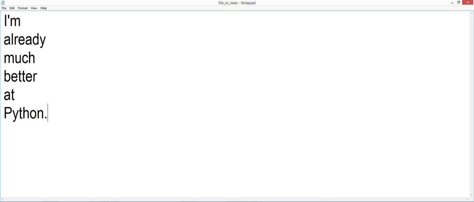
Save the file to your Desktop as file_to_read.txt.
Add the following lines of code at the bottom of first_script.py:
# READ A FILE# Read a single text fileinput_file=sys.argv[1]("Output # 143:")filereader=open(input_file,'r')forrowinfilereader:(row.strip())filereader.close()
The first line in this example uses the sys.argv list to capture the path to the file we intend to read and assigns the path to the variable input_file. The second line creates a file object, filereader, which contains the rows resulting from opening the input_file in 'r' (read) mode. The for loop in the next line reads the rows in the filereader object one at a time. The body of the for loop prints each row, and the strip function removes spaces, tabs, and newline characters from the ends of each row before it is printed. The final line closes the filereader object once all of the rows in the input file have been read and printed to the screen.
Resave first_script.py.
To read the text file, type the following line, as shown in Figure 1-11, and then hit Enter:
python first_script.py file_to_read.txt
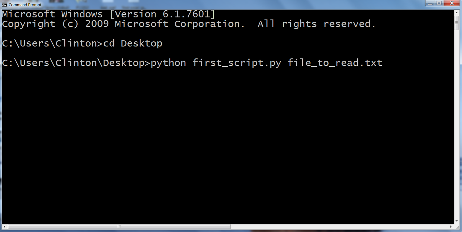
At this point, you’ve now read a text file in Python. You should see the following printed at the bottom of your screen, beneath any other previous output (Figure 1-12):
I'm
already
much
better
at
Python.
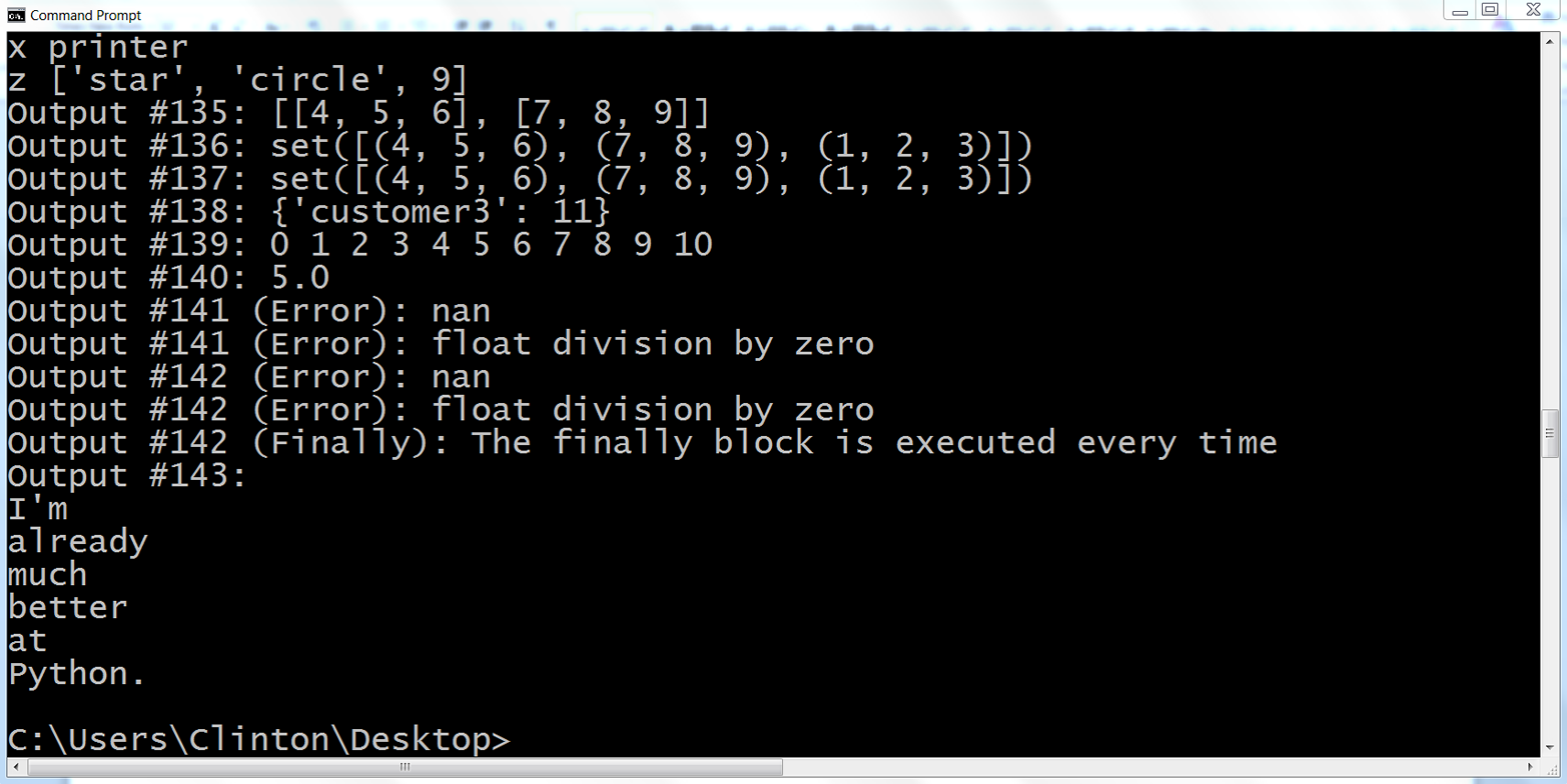
It was possible to simply type python first_script.py file_to_read.txt on the command line because first_script.py and file_to_read.txt were in the same location—that is, on your Desktop. If the text file is not in the same location as the script, then you need to supply the full path to the text file so that the script knows where to find the file.
For example, if the text file is in your Documents folder instead of on your Desktop, you can use the following path on the command line to read the text file from its alternative location:
python first_script.py "C:\Users\[Your Name]\Documents\file_to_read.txt"
The line of code we used to create the filereader object is a legacy way of creating the file object. This method works just fine, but it leaves the file object open until either it is explicitly closed with the close function or the script finishes. While this behavior isn’t usually harmful in any way, it is less clean than it could be and has been known to cause errors in more complex scripts. Since Python 2.5, you can use the with statement to create a file object instead. This syntax automatically closes the file object when the with statement is exited:
input_file=sys.argv[1]("Output #144:")withopen(input_file,'r',newline='')asfilereader:forrowinfilereader:("{}".format(row.strip()))
As you can see, the with statement version is very similar to the previous version, but it eliminates the need to include a call to the close function to close the filereader object.
This example demonstrated how to use sys.argv to access and print the contents of a single text file. It was a simple example, but we will build on it in later examples to access other types of files, to access multiple files, and to write to output files.
The next section covers the glob module, which enables you to read and process multiple input files with only a few lines of code. Because the power of the glob module comes from pointing to a folder (i.e., a directory rather than a file), let’s delete or comment out the previous file-reading code so that we can use argv[1] to point to a folder instead of to a file. Commenting out simply means putting hash symbols before every line of code you want the machine to ignore, so when you do this first_script.py should look like:
## Read a text file (older method) ###input_file = sys.argv[1]#print("Output #143:")#filereader = open(input_file, 'r', newline='')#for row in filereader:# print("{}".format(row.strip()))#filereader.close()## Read a text file (newer method) ###input_file = sys.argv[1]#print("Output #144:")#with open(input_file, 'r', newline='') as filereader:# for row in filereader:# print("{}".format(row.strip()))
With these changes, you are ready to add the glob code discussed in the next section to process multiple files.
In many business applications, the same or similar actions need to happen to multiple files. For example, you may need to select a subset of data from multiple files, calculate statistics like totals and means from multiple files, or even calculate statistics for subsets of data from multiple files. As the number of files increases, the ease of processing them manually decreases and the opportunity for errors increases.
One way to read multiple files is to include the path to the directory that contains the input files after the name of the Python script on the command line. To use this method, you need to import the built-in os and glob modules at the top of your script. To make all of the functionality provided by the os and glob modules available to you in your script, add import os and import glob at the top of your script:
#!/usr/bin/env python3frommathimportexp,log,sqrtimportrefromdatetimeimportdate,time,datetime,timedeltafromoperatorimportitemgetterimportsysimportglobimportos
When you import the os module, you have several useful pathname functions at your disposal. For example, the os.path.join function joins one or more path components together intelligently. The glob module finds all pathnames matching a specific pattern. By using os and glob in combination, you can find all files in a specific folder that match a specific pattern.
In order to read multiple text files, we need to create another text file.
Open the Spyder IDE or a text editor (e.g., Notepad, Notepad++, or Sublime Text on Windows; TextMate, TextWrangler, or Sublime Text on macOS).
Write the following eight lines in the text file (Figure 1-13):
This text comes from a different text file.
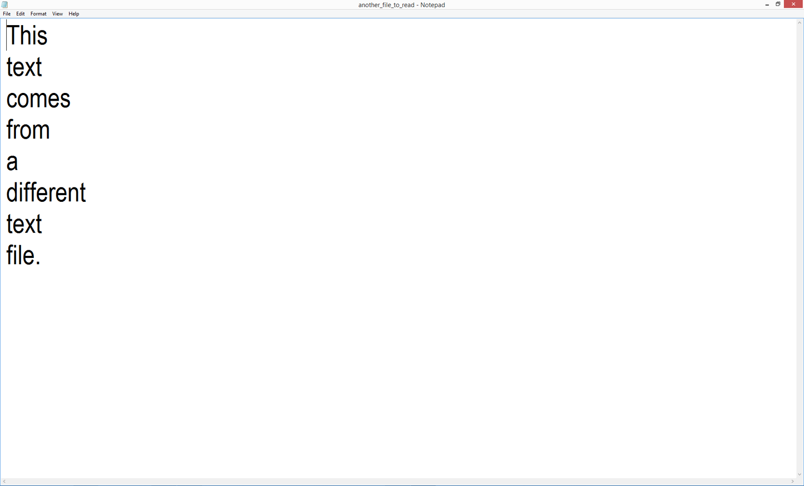
Save the file to your Desktop as another_file_to_read.txt.
Add the following lines of code at the bottom of first_script.py:
# Read multiple text files("Output #145:")inputPath=sys.argv[1]forinput_fileinglob.glob(os.path.join(inputPath,'*.txt')):withopen(input_file,'r',newline='')asfilereader:forrowinfilereader:("{}".format(row.strip()))
The first line in this example is very similar to that used in the example of reading a single text file, except that in this case we will be supplying a path to a directory instead of a path to a file. Here, we will be supplying the path to the directory that contains the two text files.
The second line is a for loop that uses the os.path.join function and the glob.glob function to find all of the files in a particular folder that match a specific pattern. The path to the particular folder is contained in the variable inputPath, which we will supply on the command line. The os.path.join function joins this folder path with all of the names of files in the folder that match the specific pattern expanded by the glob.glob function. In this case, I use the pattern *.txt to match any filename that ends with .txt. Because this is a for loop, the rest of the syntax on this line should look familiar. input_file is a placeholder name for each of the files in the list created by the glob.glob function. This line basically says, “For each file in the list of matching files, do the following…”
The remaining lines of code are the same as the lines of code used to read a single file. Open the input_file variable in read mode and create a filereader object. For each row in the filereader object, remove spaces, tabs, and newline characters from the ends of the row, and then print the row.
Resave first_script.py.
To read the text files, type the following line, as shown in Figure 1-14, and then hit Enter:
python first_script.py "C:\Users\[Your Name]\Desktop"
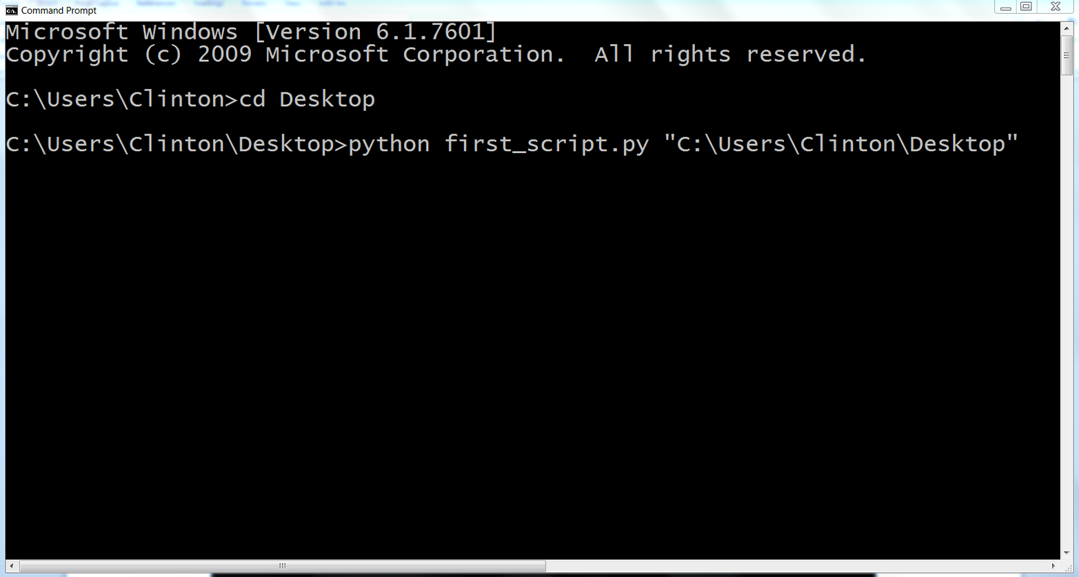
At this point, you’ve now read multiple text files in Python. You should see the following printed at the bottom of your screen, beneath any other previous output (Figure 1-15):
Thistextcomesfromadifferenttextfile.I'malreadymuchbetteratPython.
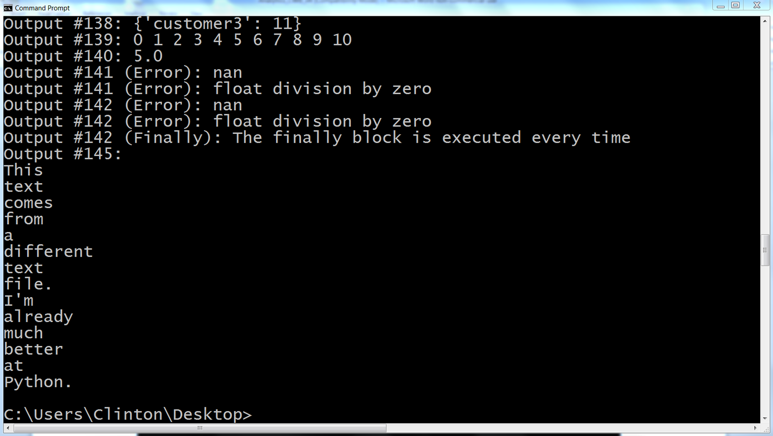
One great aspect of learning this technique is that it scales. This example involved only two files, but it could just as easily have involved dozens to hundreds or thousands or more files. By learning how to use the glob.glob function, you will be able to process a great number of files in a fraction of the time it would take to do so manually.
Most of the examples thus far have included print statements that send the output to the Command Prompt or Terminal window. Printing the output to the screen is useful when you are debugging your program or reviewing the output for accuracy. However, in many cases, once you know the output is correct, you will want to write that output to a file for further analysis, reporting, or storage.
Python provides two easy methods for writing to text and delimited files. The write method writes individual strings to a file, and the writelines method writes a sequence of strings to a file. The following two examples make use of the combination of the range and len functions to keep track of the indices of the values in a list so that the delimiter is placed between the values and a newline character is placed after the last value.
Add the following lines of code at the bottom of first_script.py:
# WRITE TO A FILE# Write to a text filemy_letters=['a','b','c','d','e','f','g','h','i','j']max_index=len(my_letters)output_file=sys.argv[1]filewriter=open(output_file,'w')forindex_valueinrange(len(my_letters)):ifindex_value<(max_index-1):filewriter.write(my_letters[index_value]+'\t')else:filewriter.write(my_letters[index_value]+'\n')filewriter.close()("Output #146: Output written to file")
In this example, the variable my_letters is a list of strings. We want to print these letters, each separated by a tab, to a text file. The one complication in this example is ensuring that the letters are printed with tabs between them and a newline character (not a tab) is placed after the final letter.
In order to know when we have reached the final letter we need to keep track of the index values of the letters in the list. The len function counts the number of values in a list, so max_index equals 10. Again, we use sys.argv[1] to supply the path to and name of the output file on the command line in the Command Prompt or Terminal window. We create a file object, filewriter, but instead of opening it for reading we open it for writing with the 'w' (write) mode. We use a for loop to iterate through the values in the list, my_letters, and we use the range function in combination with the len function to keep track of the index of each value in the list.
The if-else logic enables us to differentiate between the last letter in the list and all of the preceding letters in the list. Here is how the if-else logic works: my_letters contains ten values, but indices start at zero, so the index values for the letters are 0, 1, 2, 3, 4, 5, 6, 7, 8, 9. Therefore, my_letters[0] is a and my_letters[9] is j. The if block evaluates whether the index value x is less than nine, max_index – 1 or 10 – 1 = 9. This condition is True until the last letter in the list. Therefore, the if block says, “Until the last letter in the list, write the letter followed by a tab in the output file.” When we reach the last letter in the list the index value for that letter is 9, which is not less than 9, so the if block evaluates as False and the else block is executed. The write statement in the else block says, “Write the final letter followed by a newline character in the output file.”
Comment out the earlier code for reading multiple files.
In order to see this code in action, we need to write to a file and view the output. Because we once again are going to use argv[1] to specify the path to and name of the output file, let’s delete or comment out the previous glob code so that we can use argv[1] to specify the output file. If you choose to comment out the previous glob code, then first_script.py should look like:
## Read multiple text files#print("Output #145:")#inputPath = sys.argv[1]#for input_file in glob.glob(os.path.join(inputPath,'*.txt')):# with open(input_file, 'r', newline='') as #filereader:# for row in filereader:# print("{}".format(row.strip()))
Resave first_script.py.
To write to a text file, type the following line, as shown in Figure 1-16, and hit enter:
python first_script.py "C:\Users\[Your Name]\Desktop\write_to_file.txt"

Open the output file, write_to_file.txt.
You’ve now used Python to write output to a text file. After you complete these steps, you will not see any new output on the screen; however, if you minimize all of your open windows and look on your Desktop, there should be a new text file called write_to_file.txt. The file should contain the letters from the list my_letters separated by tabs with a newline character at the end, as seen in Figure 1-17.
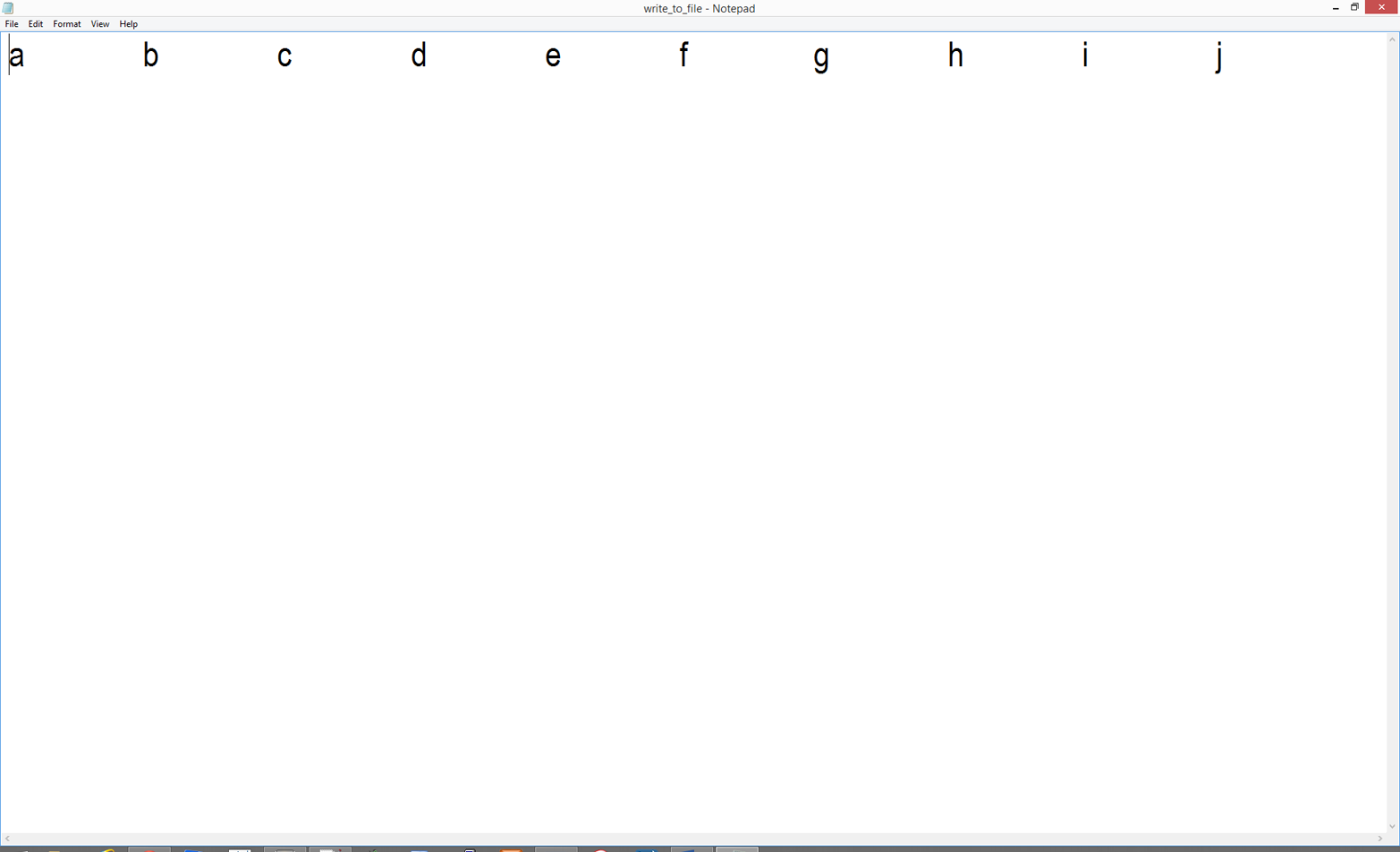
The next example is very similar to this one, except it demonstrates using the str function to convert values to strings so they can be written to a file with the write function. It also demonstrates the 'a' (append) mode to append output to the end of an existing output file.
Add the following lines of code at the bottom of first_script.py:
# Write to a CSV filemy_numbers=[0,1,2,3,4,5,6,7,8,9]max_index=len(my_numbers)output_file=sys.argv[1]filewriter=open(output_file,'a')forindex_valueinrange(len(my_numbers)):ifindex_value<(max_index-1):filewriter.write(str(my_numbers[index_value])+',')else:filewriter.write(str(my_numbers[index_value])+'\n')filewriter.close()"Output #147: Output appended to file"
This example is very similar to the preceding one, but it demonstrates how to append to an existing output file and how to convert non-string values in a list into strings so they can be written to a file with the write function. In this example, the list contains integers. The write function writes strings, so you need to use the str function to convert the non-string values into strings before they can be written to the output file with the write function.
In the first iteration through the for loop, the str function will write a zero to the output file, followed by a single comma. Writing each of the numbers in the list to the output file continues in this way until the last number in the list, at which point the else block is executed and the final number is written to the file followed by a newline character instead of a comma.
Notice that we opened the file object, filewriter, in append mode ('a') instead of write mode ('w'). If we supply the same output filename on the command line, then the output of this code will be appended below the output previously written to write_to_file.txt. Alternatively, if we opened filewriter in write mode, then the previous output would be deleted and only the output of this code would appear in write_to_file.txt. You will see the power of opening a file object in append mode later in this book when we process multiple files and append all of the data together into a single, concatenated output file.
Resave first_script.py.
To append to the text file, type the following line and then hit Enter:
python first_script.py "C:\Users\[Your Name]\Desktop\write_to_file.txt"
Open the output file, write_to_file.txt.
You’ve now used Python to write and append output to a text file. After you complete these steps, you will not see any new output printed to the screen; however, if you open write_to_file.txt you’ll see that there’s now a new second line that contains the numbers in my_numbers separated by commas with a newline character at the end, as shown in Figure 1-18.
Finally, this example demonstrates an effective way for writing CSV files. In fact, if we did not write the output from the previous tab-based example to the output file (that output was separated by tabs instead of by commas) and we named the file write_to_file.csv instead of write_to_file.txt, then we would have created a CSV file.
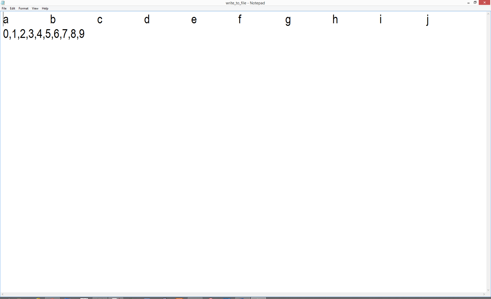
print statements are an important aid to debugging any program. As you have seen, many of the examples in this chapter included print statements as output. However, you can also add print statements in your code temporarily to see intermediate output. If your code is not working at all or is not producing the results you expect, then start adding print statements in meaningful locations from the top of your program to see if the initial calculations are what you expect. If they are, continue down through subsequent lines of code to check that they are also working as expected.
By starting at the top of your script, you can ensure that you identify the first place where the results are in error and fix the code at that point before testing the remaining sections of your code. The message of this brief section is, “Don’t be afraid to use print statements liberally throughout your code to help you debug your code and ensure it’s working properly!” You can always comment out or remove the print statements later when you are confident your code is working properly.
We’ve covered a lot of ground in this chapter. We’ve discussed how to import modules, basic data types and their functions and methods, pattern matching, print statements, dates, control flow, functions, exceptions, reading single and multiple files, as well as writing text and delimited files. If you’ve followed along with the examples in this chapter, you have already written over 500 lines of Python code!
The best part about all of the work you have put into working through the examples in this chapter is that they are the basic building blocks for doing more complex file processing and data manipulation. Having worked through the examples in this chapter, you’re now well prepared to understand and master the techniques demonstrated in the remaining chapters in this book.
Example solutions can be found in Appendix B.
Create a new Python script. In it, create three different lists, add the three lists together, and use a for loop and positional indexing (i.e., range(len())) to loop through the list and print the index values and elements in the list to the screen.
Create a new Python script. In it, create two different lists of equal length. One of the lists must contain unique strings. Also create an empty dictionary. Use a for loop, positional indexing, and an if statement to test whether each of the values in the list of unique strings is already a key in the dictionary. If it is not, then add the value as a key and add the value in the other list that has the same index position as the key’s associated value. Print the dictionary’s keys and values to the screen.
Create a new Python script. In it, create a list of equal-length lists. Modify the code used in “Writing to a Comma-Separated Values (CSV) File” to loop through the list of lists and print the values in each of the lists to the screen as a string of comma-separated values with a newline character at the end.
The comma-separated values (CSV) file format is a very simple way of storing and sharing data. CSV files hold data tables as plain text; each cell of the table (or spreadsheet) is just a number or string. One of the principal advantages of a CSV file compared to an Excel file is that there are many programs capable of storing, transferring, and processing plain-text files; on the other hand, there are fewer that are capable of handling Excel files. Any spreadsheet program, word processor, or simple text editor can handle plain-text files, but not all of them can handle Excel files. While Excel is an incredibly powerful tool, when you work with Excel files, you’re basically limited to the tasks that Excel can perform. CSV files give you the freedom to send your data to the right tool for the job you want to do—or to build your own tools using Python!
You do lose some of Excel’s features when you work with CSV files: whereas every cell of an Excel spreadsheet has a defined “type” (number, text, currency, date, etc.), cells of CSV files are just raw data. Thankfully, Python is pretty clever about recognizing different data types, as we’ve seen in Chapter 1. Another trade-off with using CSV files is that they don’t store formulas, only data. However, by separating the data storage (CSV file) and data processing (Python script), you make it easier to apply your processing to different datasets. It’s also easier to find—and harder to propagate!—errors (in both the processing and the data files) when the processing and storage are separate.
In order to begin working with this format, you’ll need to create a CSV file (you can also download this file from https://github.com/cbrownley/foundations-for-analytics-with-python/blob/master/csv/supplier_data.csv):
Open a new spreadsheet and add the data as shown in Figure 2-1.
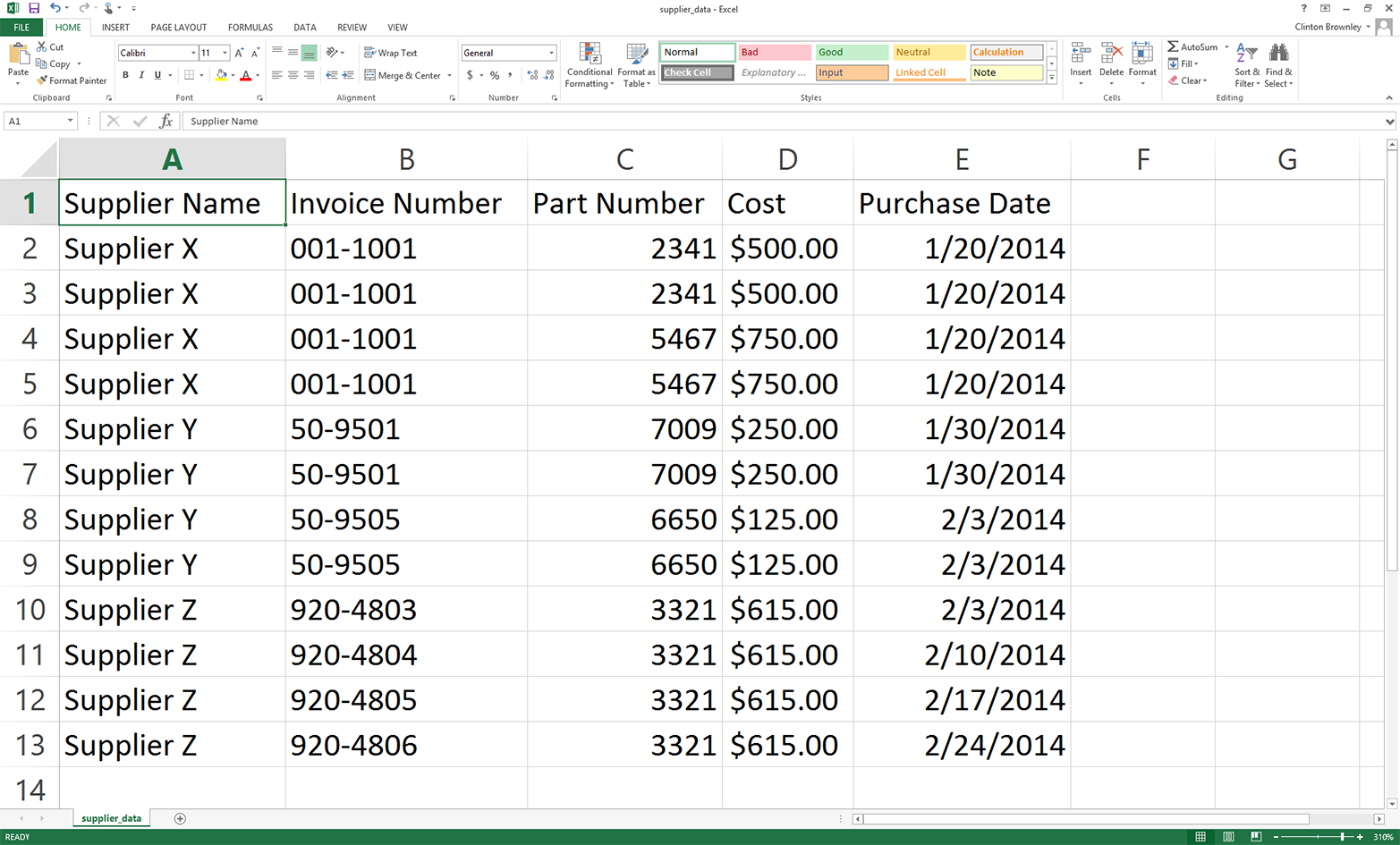
Save the file to your Desktop as supplier_data.csv.
To confirm that supplier_data.csv is indeed a plain-text file:
Minimize all of your open windows and locate supplier_data.csv on your Desktop.
Right-click the file.
Select “Open with” and then select a text editor like Notepad, Notepad++, or Sublime Text.
When you open the file in the text editor, it should look like what is shown in Figure 2-2.
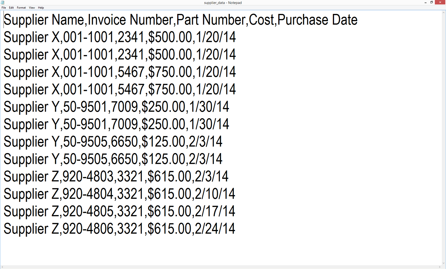
As you can see, the file is simply a plain-text file. Each row contains five values separated by commas. Another way to think about it is that the commas delineate the five columns in the Excel spreadsheet. You can now close the file.
As mentioned in the Preface, each of the subsections in this chapter presents two versions of code to accomplish a specific data processing task. The first version of code in each subsection shows how to accomplish the task with base Python. The second version shows how to accomplish it with pandas. As you’ll see, pandas makes it easy to accomplish a task with relatively few lines of code, so it’s very useful for simply getting the job done or for accomplishing the task once you understand the programming concepts and operations it’s simplifying for you. However, I start each subsection with the base Python version so you learn how to accomplish the specific task with general programming concepts and operations. By presenting both versions, I want to give you the option to quickly get the job done with pandas or learn general programming and problem-solving skills you can build on as you develop your coding skills. I won’t explain the pandas versions in quite as much detail as the base Python versions; you can use the examples here as a “cookbook” to get the job done with pandas, but if you want to become a pandas power user after you work your way through this book, I recommend Wes McKinney’s Python for Data Analysis (O’Reilly) as a next step.
Now let’s learn how to read, process, and write a CSV file in base Python (without using the built-in csv module). By seeing this example first, you’ll then have an idea of what’s going on “under the hood” when you use the csv module.
To work with our CSV file, let’s create a new Python script, 1csv_read_with_simple_parsing_and_write.py.
Type the following code into Spyder or a text editor:
1#!/usr/bin/env python32importsys3 4input_file=sys.argv[1]5output_file=sys.argv[2]6 7withopen(input_file,'r',newline='')asfilereader:8withopen(output_file,'w',newline='')asfilewriter:9header=filereader.readline()10header=header.strip()11header_list=header.split(',')12(header_list)13filewriter.write(','.join(map(str,header_list))+'\n')14forrowinfilereader:15row=row.strip()16row_list=row.split(',')17(row_list)18filewriter.write(','.join(map(str,row_list))+'\n')
Save the script to your Desktop as 1csv_read_with_simple_parsing_and_write.py.
Figures 2-3, 2-4, and 2-5 show what the script looks like in Anaconda Spyder, Notepad++ (Windows), and TextWrangler (macOS), respectively.
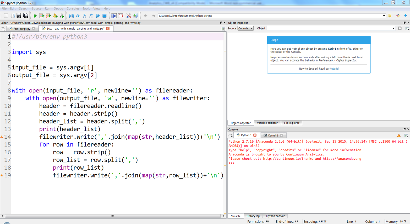
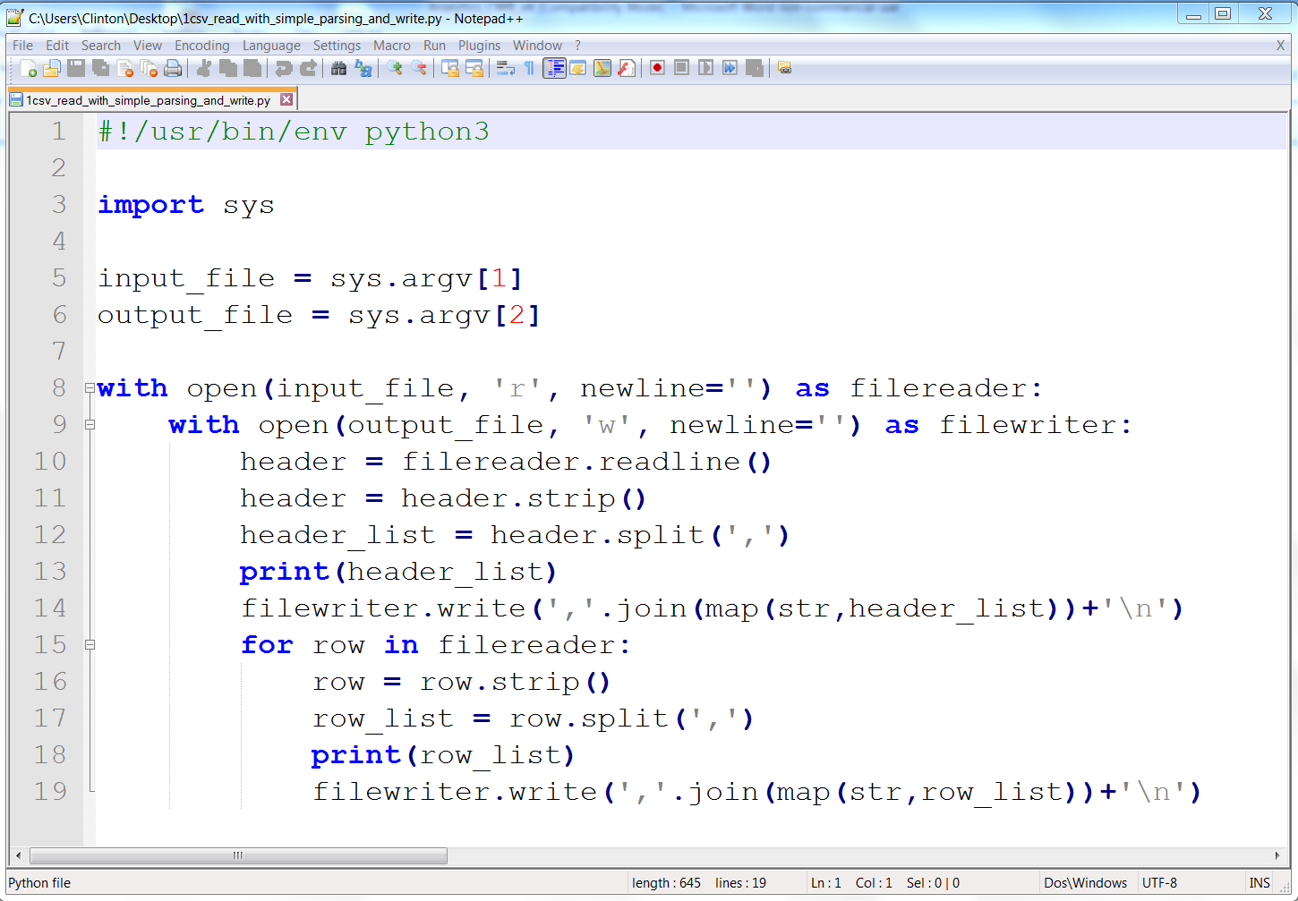
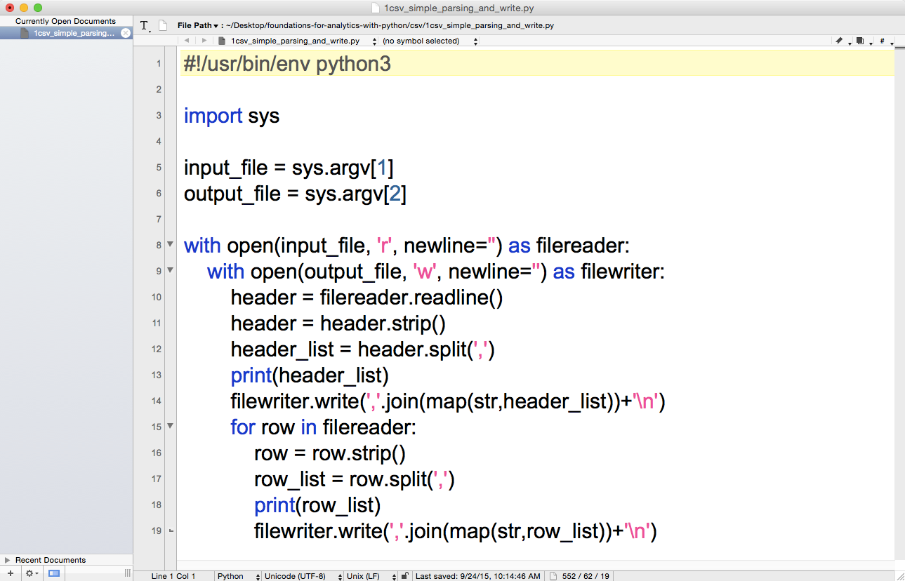
Before we run this script and view the output, let’s explore what the code in the script is supposed to do. We’ll discuss each of the blocks of code in turn (the line numbers refer to the line numbers shown in the screenshots):
#!/usr/bin/env python3importsys
As we discussed in Chapter 1, line 1 is a comment line that makes the script transferable across operating systems. Line 2 imports Python’s built-in sys module, which enables you to send additional input to your script from the command line.
input_file=sys.argv[1]output_file=sys.argv[2]
Lines 4 and 5 use the sys module’s argv parameter, which is the list of command-line arguments passed to a Python script—that is, what you enter at the command line at the time you run the script. Here is a generic version of the command-line arguments we’ll use to read a CSV input file and write a CSV output file on a Windows computer:
python script_name.py "C:\path\to\input_file.csv" "C:\path\to\output_file.csv"
The first word, python, tells your computer to use the Python program to process the rest of the command-line arguments. Python collects the rest of the arguments into a special list called argv. It reserves the first position in the list, argv[0], for the script name, so argv[0] refers to script_name.py. The next command-line argument is "C:\path\to\input_file.csv", the path to and name of the CSV input file. Python stores this value in argv[1], so line 4 in our script assigns this value to the variable named input_file. The last command-line argument is "C:\path\to\output_file.csv", the path to and name of the CSV output file. Python stores this value in argv[2] and line 5 assigns this value to the variable named output_file.
withopen(input_file,'r',newline='')asfilereader:withopen(output_file,'w',newline='')asfilewriter:
Line 7 is a with statement that opens input_file as a file object, filereader. The 'r' specifies read mode, which means input_file is opened for reading. Line 8 is another with statement that opens output_file as a file object, filewriter. The 'w' specifies write mode, which means output_file is opened for writing. As we saw in “Modern File-Reading Syntax”, the with syntax is helpful because it automatically closes the file object when the with statement is exited.
header=filereader.readline()header=header.strip()header_list=header.split(',')
Line 9 uses the file object’s readline method to read in the first line of the input file, which in this case is the header row, as a string and assigns it to a variable named header. Line 10 uses the string module’s strip function to remove spaces, tabs, and newline characters from both ends of the string in header and reassigns the stripped version of the string to header. Line 11 uses the string module’s split function to split the string on commas into a list, where each value in the list is a column heading, and assigns the list to a variable named header_list.
(header_list)filewriter.write(','.join(map(str,header_list))+'\n')
Line 12 is a print statement that prints the values in header_list (i.e., the column headings) to the screen.
Line 13 uses the filewriter object’s write method to write each of the values in header_list to the output file. Because there is a lot going on in this one line, let’s inspect it from the inside out. The map function applies the str function to each of the values in header_list to ensure each of the values is a string. Then the join function inserts a comma between each of the values in header_list and converts the list into a string. Next, a newline character is added to the end of the string. Finally, the filewriter object writes the string as the first row in the output file.
forrowinfilereader:row=row.strip()row_list=row.split(',')(row_list)filewriter.write(','.join(map(str,row_list))+'\n')
Line 14 creates a for loop to iterate through the remaining rows in the input file. Line 15 uses the strip function to remove spaces, tabs, and newline characters from both ends of the string in row and reassigns the stripped version of the string to row. Line 16 uses the split function to split the string on commas into a list, where each value in the list is a column value from the row, and assigns the list to a variable named row_list. Line 17 prints the values in row_list to the screens and line 18 writes the values to the output file.
The script executes lines 15 to 18 for every row of data in the input file, as these four lines are indented beneath the for loop in line 14.
You can test out the script by running it in a Command Prompt or Terminal window, as described next:
Open a Command Prompt window.
Navigate to your Desktop (where you saved the Python script).
To do so, type the following line and then hit Enter:
cd"C:\Users\[Your Name]\Desktop"
Run the Python script.
To do so, type the following line and then hit Enter:
python 1csv_simple_parsing_and_write.py supplier_data.csv\ output_files\1output.csv
Open a Terminal window.
Navigate to your Desktop (where you saved the Python script).
To do so, type the following line and then hit Enter:
cd /Users/[Your Name]/Desktop
Make the Python script executable.
To do so, type the following line and then hit Enter:
chmod +x 1csv_simple_parsing_and_write.py
Run the Python script.
To do so, type the following line and then hit Enter:
./1csv_simple_parsing_and_write.py supplier_data.csv\ output_files/1output.csv
You should see the output shown in Figure 2-6 printed to the Command Prompt or Terminal window.
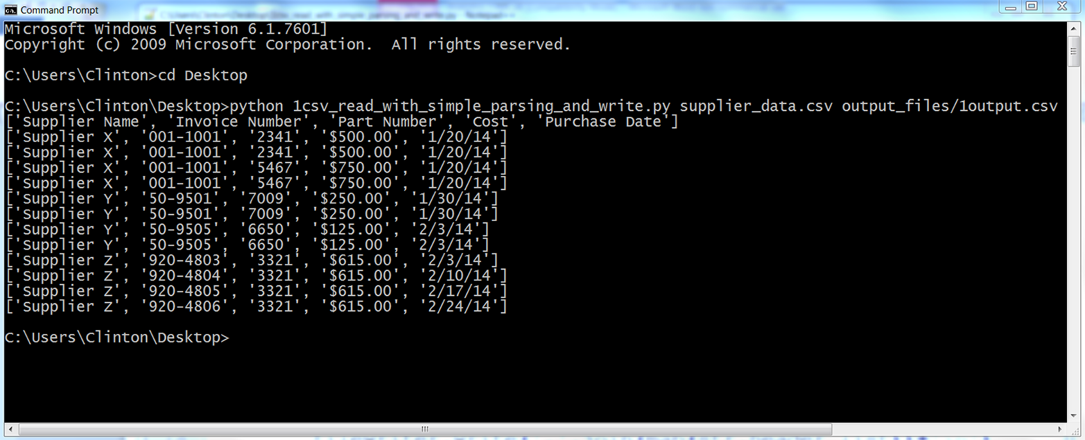
All of the rows in the input file have been printed to the screen and written to the output file. In most cases, you do not need to rewrite all of the data from an input file to an output file because you already have all of the data in the input file, but this example is useful because it foreshadows how you can embed the filewriter.write statement in conditional business logic to ensure you only write specific rows of interest to the output file.
To process a CSV file with pandas, type the following code into a text editor and save the file as pandas_parsing_and_write.py (this script reads a CSV file, prints the contents to the screen, and writes the contents to an output file):
#!/usr/bin/env python3importsysimportpandasaspdinput_file=sys.argv[1]output_file=sys.argv[2]data_frame=pd.read_csv(input_file)(data_frame)data_frame.to_csv(output_file,index=False)
To run the script, type one of the following commands on the command line, depending on your operating system:
python pandas_parsing_and_write.py supplier_data.csv\ output_files\pandas_output.csv
chmod +x pandas_parsing_and_write.py ./pandas_parsing_and_write .py supplier_data.csv\ output_files/pandas_output.csv
You’ll note that in the pandas version of the script, we created a variable called data_frame. Like lists, dictionaries, and tuples, DataFrames are a way to store data. They preserve the “table” organization of your data without having to parse the data as a list of lists. DataFrames are part of the pandas package; they don’t exist unless you’ve imported pandas as part of your script. While we called the variable data_frame, that’s like using the variable name list—it’s useful at the learning stage, but you’ll probably want to use more descriptive variable names in the future.
One way basic CSV parsing can fail is when column values contain extra commas. Open supplier_data.csv and make the last two cost amounts in the Cost column $6,015.00 and $1,006,015.00, respectively. With these two changes, the input file should look as shown in Figure 2-7.
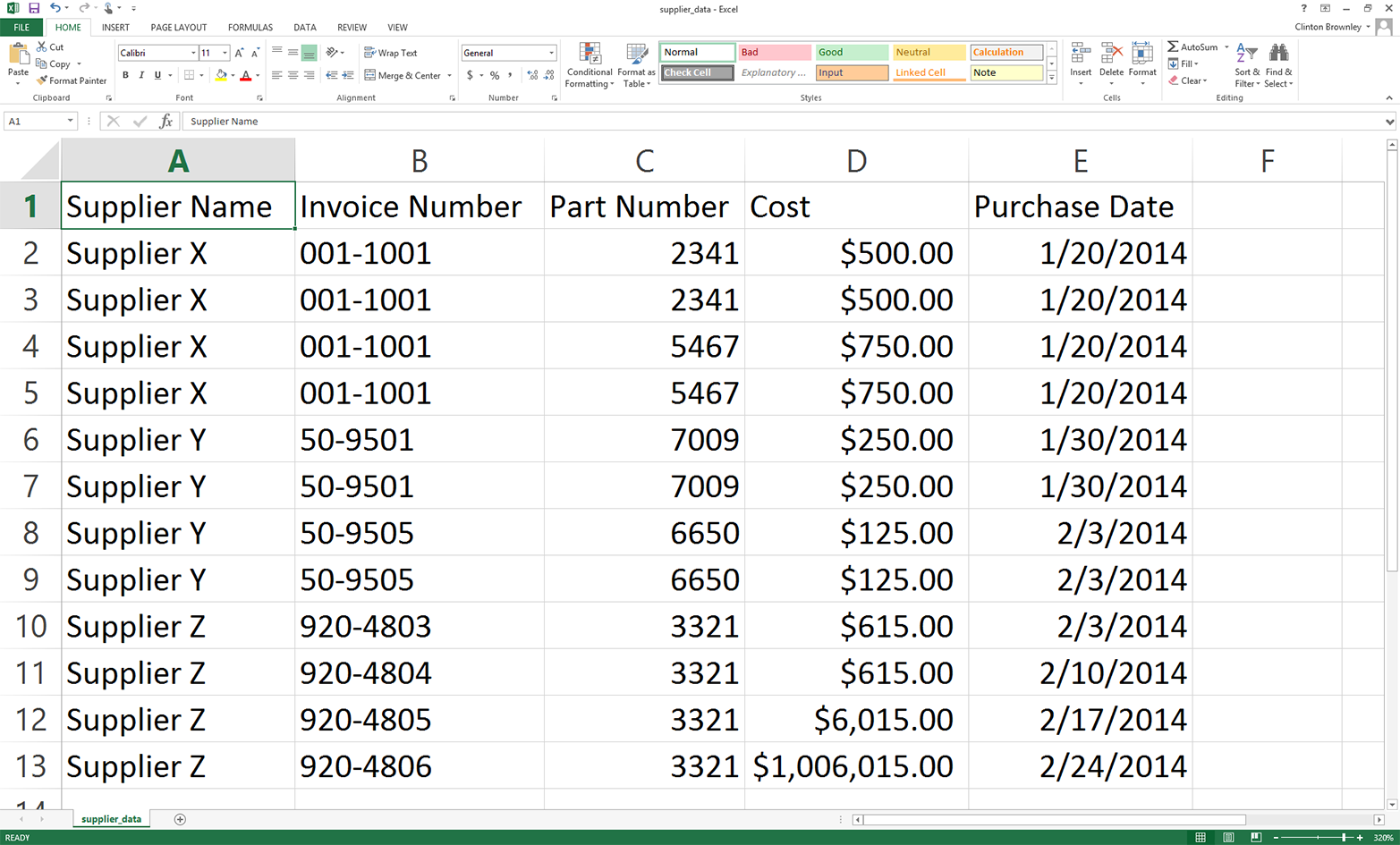
To see how our simple parsing script fails after changing the input file, rerun the script on the new, modified input file. That is, save the file with these changes, then hit the up arrow to recover the previous command you ran or retype the following command and hit Enter:
python 1csv_simple_parsing_and_write.py supplier_data.csv\ output_files\1output.csv
You should see the output shown in Figure 2-8 printed to the screen.
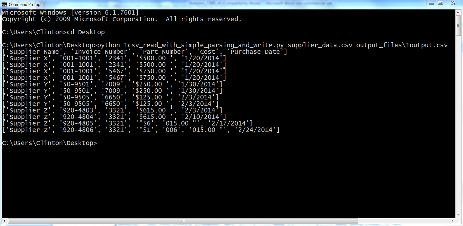
As you can see, our script parsed each row based on the commas in the row. The script handled the header row and the first 10 data rows correctly because they did not include embedded commas. However, the script split the last two rows incorrectly because they did include embedded commas.
There are many ways to enhance the code in this script to handle values that contain embedded commas. For example, we could use a regular expression to search for patterns with embedded commas like $6,015.00 and $1,006,015.00 and then remove the commas in these values before splitting the row on the remaining commas. However, instead of complicating our script, let’s use Python’s built-in csv module, which is designed to handle arbitrarily complex CSV files.
One of the advantages of using Python’s built-in csv module to process CSV files is that it has been designed to properly handle embedded commas and other complex patterns in data values. It recognizes these patterns and parses the data correctly so you can spend your time managing the data, performing calculations, and writing output instead of designing regular expressions and conditional logic just to properly ingest your data.
Let’s import Python’s built-in csv module and use it to process the version of the input file that contains the numbers $6,015.00 and $1,006,015.00. You’ll learn how to use the csv module and see how it handles commas within data items.
Type the following code into a text editor and save the file as 2csv_reader_parsing_and_write.py:
1#!/usr/bin/env python32importcsv3importsys4input_file=sys.argv[1]5output_file=sys.argv[2]6withopen(input_file,'r',newline='')ascsv_in_file:7withopen(output_file,'w',newline='')ascsv_out_file:8filereader=csv.reader(csv_in_file,delimiter=',')9filewriter=csv.writer(csv_out_file,delimiter=',')10forrow_listinfilereader:11(row_list)12filewriter.writerow(row_list)
As you can see, most of this code is similar to the code we wrote in the first version of this script. Therefore, I’ll only discuss the lines that are significantly different.
Line 2 imports the csv module so we can use its functions to parse the input file and write to an output file.
Line 8, the line beneath the second with statement, uses the csv module’s reader function to create a file reader object named filereader that we’ll use to read the rows in the input file. Similarly, line 9 uses the csv module’s writer function to create a file writer object called filewriter that we’ll use to write to an output file. The second argument in these functions (i.e., delimiter=',') is the default delimiter, so you do not need to include it if your input and output files are comma-delimited. I included the delimiter arguments in case you need to process an input file that has a different column delimiter or write to an output file with a different delimiter—for example, a semicolon (;) or tab (\t).
Line 12 uses the filewriter object’s writerow function to write the list of values in each row to the output file.
Assuming the input file and Python script are both saved on your Desktop and you have not changed directories in the Command Prompt or Terminal window, type the following on the command line and then hit Enter to run the script (if you are on a Mac, you’ll first need to run the chmod command on the new script to make it executable):
python 2csv_reader_parsing_and_write.py supplier_data.csv\ output_files\2output.csv
You should see the output shown in Figure 2-9 printed to the screen.
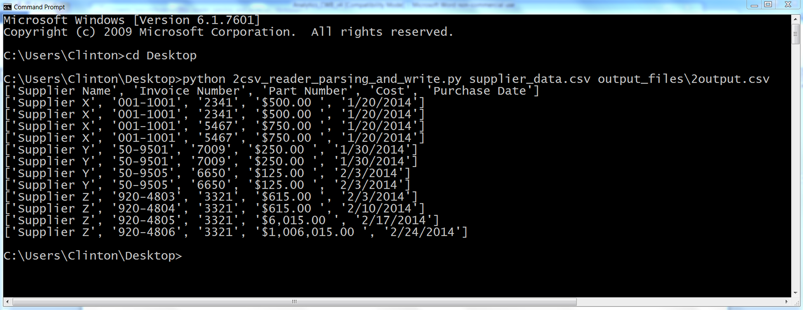
All of the rows in the input file have been printed to the screen and written to the output file. As you can see, Python’s built-in csv module handled the embedded commas for us and correctly parsed every row into a list with five values.
Now that we know how to use the csv module to read, process, and write CSV files, let’s learn how to filter for specific rows and select specific columns so we can effectively extract the data we need.
Sometimes a file contains more rows than you need. For example, you may only need a subset of rows that contain a specific word or number, or you may only need a subset of rows associated with a specific date. In these cases, you can use Python to filter for the specific rows you want to retain.
You may be familiar with how to filter rows manually in Excel, but the focus of this chapter is to broaden your capabilities so you can deal with CSV files that are too large to open in Excel and collections of CSV files that would be too time consuming to deal with manually.
The following subsections demonstrate three different ways to filter for specific rows in an input file:
Value in row meets a condition
Value in row is in a set of interest
Value in row matches a pattern of interest (regular expression)
You will notice that the code in these subsections has a consistent structure or format. I want to point out this common structure so it’s easy for you to identify where to modify the code to incorporate your own business rules.
Focus on the following structure in the next three subsections to understand how to filter for specific rows in an input file:
forrowinfilereader:***ifvalueinrowmeetssomebusinessruleorsetofrules:***dosomethingelse:dosomethingelse
This pseudocode shows the common structure of the code we’ll use to filter for specific rows in an input file. In the following subsections, we’ll see how to modify the line enclosed in *** to incorporate specific business rules and extract the rows you need.
Sometimes you need to retain rows where a value in the row meets a specific condition. For example, you may want to retain all of the rows in our dataset where the cost is above a specific threshold. Or you may want all of the rows where the purchase date is before a specific date. In these cases, you can test the row value against the specific condition and filter for the rows that meet the condition.
The following example demonstrates how to test row values against two conditions and write the subset of rows that meet the conditions to an output file. In this example, we want to retain the subset of rows where the supplier name is Supplier Z or the cost is greater than $600.00 and write the results to an output file. To filter for the subset of rows that meet these conditions, type the following code into a text editor and save the file as 3csv_reader_value_meets_condition.py:
1#!/usr/bin/env python32importcsv3importsys4input_file=sys.argv[1]5output_file=sys.argv[2]6withopen(input_file,'r',newline='')ascsv_in_file:7withopen(output_file,'w',newline='')ascsv_out_file:8filereader=csv.reader(csv_in_file)9filewriter=csv.writer(csv_out_file)10header=next(filereader)11filewriter.writerow(header)12forrow_listinfilereader:13supplier=str(row_list[0]).strip()14cost=str(row_list[3]).strip('$').replace(',','')15ifsupplier=='Supplier Z'orfloat(cost)>600.0:16filewriter.writerow(row_list)
Line 10 uses the csv module’s next function to read the first row in the input file into a list variable named header. Line 11 writes the header row to the output file.
Line 13 grabs the supplier’s name in each row and assigns it to a variable named supplier. It uses list indexing to grab the first value in each row, row[0], then it uses the str function to convert the value into a string. Next, it uses the strip function to remove spaces, tabs, and newline characters from the ends of the string. Finally, it assigns this stripped string to the variable supplier.
Line 14 grabs the cost value in each row and assigns it to a variable named cost. It uses list indexing to grab the fourth value in each row, row[3], then it uses the str function to convert the value into a string. Net, it uses the strip function to remove the dollar sign from the string. Then it uses the replace function to remove commas from the string. Finally, it assigns the resulting string to the variable cost.
Line 15 creates an if statement to test two values in each row against two conditions. Specifically, we want to filter for rows where the supplier name is Supplier Z or the cost is greater than $600.00. The first condition, between if and or, tests whether the value in the variable named supplier evaluates to Supplier Z. The second condition, between or and the colon, tests whether the value in the variable named cost, converted to a floating-point number, is greater than 600.0.
Line 16 uses the filewriter’s writerow function to write the rows that meet the conditions to the output file.
To run the script, type the following on the command line and hit Enter:
python 3csv_reader_value_meets_condition.py supplier_data.csv\ output_files\3output.csv
You won’t see any output printed to the screen, but you can open the output file, 3output.csv, to review the results. Check to make sure that they’re what you wanted—and then try modifying the code to give a different selection of data, specifying a different supplier or price threshold.
Pandas provides the loc function for selecting specific rows and columns at the same time. You specify the row filtering condition before the comma and the column filtering condition after the comma. The conditions inside the following loc function specify that we want the rows where the name in the Supplier Name column contains a Z or the amount in the Cost column is greater than 600.0, and we want all of the columns. Type the following code into a text editor and save the file as pandas_value_meets_condition.py (this script uses pandas to parse a CSV file and write the rows that meet the conditions to an output file):
#!/usr/bin/env python3importpandasaspdimportsysinput_file=sys.argv[1]output_file=sys.argv[2]data_frame=pd.read_csv(input_file)data_frame['Cost']=data_frame['Cost'].str.strip('$').astype(float)data_frame_value_meets_condition=data_frame.loc[(data_frame['Supplier Name']\.str.contains('Z'))|(data_frame['Cost']>600.0),:]data_frame_value_meets_condition.to_csv(output_file,index=False)
Run the script from the command line, supplying the source and output files for your data:
python pandas_value_meets_condition.py supplier_data.csv\ output_files\pandas_output.csv
You won’t see any output printed to the screen, but you can open the output file, pandas_output.csv, to review the results. Play around with the parameters in the loc function to create different selections of your data.
Sometimes you need to retain rows where a value in the row is in a set of interest. For example, you may want to retain all of the rows in our dataset where the supplier name is in the set {Supplier X, Supplier Y}. (These curly braces refer to set notation, not Python’s dictionary data structure.) Or you may want all of the rows where the purchase date is in the set {'1/20/14', '1/30/14'}. In these cases, you can test whether the row values are in the set and filter for rows with values in the set.
The following example demonstrates how to test row values against set membership and write the subset of rows with a value in the set to an output file. In this example, we want to retain the subset of rows where the purchase date is in the set {'1/20/14', '1/30/14'} and write the results to an output file. To filter for the subset of rows with values in this set, type the following code into a text editor and save the file as 4csv_reader_value_in_set.py:
1#!/usr/bin/env python32importcsv3importsys4input_file=sys.argv[1]5output_file=sys.argv[2]6important_dates=['1/20/14','1/30/14']7withopen(input_file,'r',newline='')ascsv_in_file:8withopen(output_file,'w',newline='')ascsv_out_file:9filereader=csv.reader(csv_in_file)10filewriter=csv.writer(csv_out_file)11header=next(filereader)12filewriter.writerow(header)13forrow_listinfilereader:14a_date=row_list[4]15ifa_dateinimportant_dates:16filewriter.writerow(row_list)
Line 6 creates a list variable named important_dates that contains the two dates of interest. This variable defines our set. It is helpful to create a variable that contains your values of interest and then reference the variable in your code. That way, if the values of interest change, you only have to make a change in one place (i.e., where you define the variable), and those changes will propagate throughout your code wherever you reference the variable.
Line 14 grabs the purchase date in each row and assigns the value to a variable named a_date. You can see from the row list’s index value, row[4], that the purchase date is in the fifth column.
Line 15 creates an if statement to test whether the purchase date in the variable named a_date is in the set of interest defined by important_dates. If the value is in the set of interest, the next line writes the row to the output file.
Run this script at the command line:
python 4csv_reader_value_in_set.py supplier_data.csv output_files/4output.csv
You can then open the output file, 4output.csv, to review the results.
To filter for rows with values in a set of interest with pandas, type the following code into a text editor and save the file as pandas_value_in_set.py (this script parses a CSV file and writes the rows with values in the set of interest to an output file):
#!/usr/bin/env python3importpandasaspdimportsysinput_file=sys.argv[1]output_file=sys.argv[2]data_frame=pd.read_csv(input_file)important_dates=['1/20/14','1/30/14']data_frame_value_in_set=data_frame.loc[data_frame['Purchase Date'].\isin(important_dates),:]data_frame_value_in_set.to_csv(output_file,index=False)
The key new command here is the very succinct isin.
As before, we’ll run the script from the command line, supplying source and output filenames:
python pandas_value_in_set.py supplier_data.csv output_files\pandas_output.csv
You can then open the output file, pandas_output.csv, to review the results.
Sometimes you need to retain a subset of rows where a value in the row matches or contains a specific pattern (i.e., regular expression). For example, you may want to retain all of the rows in our dataset where the invoice number starts with “001-”. Or you may want all of the rows where the supplier name contains a “Y”. In these cases, you can test whether the row values match or contain the pattern and filter for rows with values that do.
The following example demonstrates how to test values against a specific pattern and write the subset of rows with a value that matches the pattern to an output file. In this example, we want to retain the subset of rows where the invoice number starts with “001-” and write the results to an output file. To filter for the subset of rows with values that match this pattern, type the following code into a text editor and save the file as 5csv_reader_value_matches_pattern.py:
1#!/usr/bin/env python32importcsv3importre4importsys5input_file=sys.argv[1]6output_file=sys.argv[2]7pattern=re.compile(r'(?P<my_pattern_group>^001-.*)',re.I)8withopen(input_file,'r',newline='')ascsv_in_file:9withopen(output_file,'w',newline='')ascsv_out_file:10filereader=csv.reader(csv_in_file)11filewriter=csv.writer(csv_out_file)12header=next(filereader)13filewriter.writerow(header)14forrow_listinfilereader:15invoice_number=row_list[1]16ifpattern.search(invoice_number):17filewriter.writerow(row_list)
Line 3 imports the regular expression (re) module so that we have access to the re module’s functions.
Line 7 uses the re module’s compile function to create a regular expression variable named pattern. If you read Chapter 1, then the contents of this function will look familiar. The r says to consider the pattern between the single quotes as a raw string.
The ?P<my_pattern_group> metacharacter captures the matched substrings in a group called <my_pattern_group> so that, if necessary, they can be printed to the screen or written to a file.
The actual pattern we are searching for is ^001-.*. The caret is a special character that says to only search for the pattern at the beginning of the string. So, the string needs to start with “001-”. The period . matches any character except a newline. So, any character except a newline can come after the “001-”. Finally, the * says to repeat the preceding character restriction zero or more times. Together, the .* combination is used to say that any characters except a newline can show up any number of times after the “001-”. To say it even more informally, “The string can contain anything after the ‘-’ and as long as the string starts with ‘001-’ it will match the regular expression.”
Finally, the re.I argument instructs the regular expression to perform case-insensitive matching. This argument is less critical in this example because the pattern is numeric, but it illustrates where to include the argument if your pattern contains characters and you want to perform case-insensitive matching.
Line 15 uses list indexing to extract the invoice number from the row and assigns it to a variable named invoice_number. In the next line, we’re going to look for the pattern in this variable.
Line 16 uses the re module’s search function to look for the pattern in the value stored in invoice_number. If the pattern appears in the value in invoice_number, then line 17 writes the row to the output file.
To run the script, type the following on the command line and hit Enter:
python 5csv_reader_value_matches_pattern.py supplier_data.csv\ output_files\5output.csv
You can then open the output file, 5output.csv, to review the results.
To filter for rows with values that match a pattern with pandas, type the following code into a text editor and save the file as pandas_value_matches_pattern.py (this script reads a CSV file, prints the rows with values that match the pattern to the screen, and writes the same rows to an output file):
#!/usr/bin/env python3importpandasaspdimportsysinput_file=sys.argv[1]output_file=sys.argv[2]data_frame=pd.read_csv(input_file)data_frame_value_matches_pattern=data_frame.loc[data_frame['Invoice Number'].\str.startswith("001-"),:]data_frame_value_matches_pattern.to_csv(output_file,index=False)
With pandas, we can use startswith to find our data rather than the more cumbersome regular expression. To run the script, type the following on the command line and hit Enter:
python pandas_value_matches_pattern.py supplier_data.csv\ output_files\pandas_output.csv
You can then open the output file, pandas_output.csv, to review the results.
Sometimes a file contains more columns than you need to retain. In this case, you can use Python to select only the columns that you need.
There are two common ways to select specific columns in a CSV file. The following sections demonstrate these two methods:
Using column index values
Using column headings
One way to select specific columns in a CSV file is to use the index values of the columns you want to retain. This method is effective when it is easy to identify the index values of the columns you want to retain or, when you’re processing multiple input files, when the positions of the columns are consistent (i.e., don’t change) across all of the input files. For instance, if you only need to retain the first and last columns of data, then you could use row[0] and row[-1] to write the first and last values in each row to a file.
In this example, we only want to retain the Supplier Name and Cost columns. To select these two columns using index values, type the following code into a text editor and save the file as 6csv_reader_column_by_index.py:
1#!/usr/bin/env python32importcsv3importsys4input_file=sys.argv[1]5output_file=sys.argv[2]6my_columns=[0,3]7withopen(input_file,'r',newline='')ascsv_in_file:8withopen(output_file,'w',newline='')ascsv_out_file:9filereader=csv.reader(csv_in_file)10filewriter=csv.writer(csv_out_file)11forrow_listinfilereader:12row_list_output=[]13forindex_valueinmy_columns:14row_list_output.append(row_list[index_value])15filewriter.writerow(row_list_output)
Line 6 creates a list variable named my_columns that contains the index values of the two columns we want to retain. In this example, these two index values correspond to the Supplier Name and Cost columns. Again, it is helpful to create a variable that contains your index values of interest and then reference the variable in your code. That way, if the index values of interest change you only have to make a change in one place (i.e., where you define my_columns), and the changes will propagate throughout your code wherever you reference my_columns.
Lines 12 through 15 are indented beneath the outer for loop, so they are run for every row in the input file. Line 12 creates an empty list variable called row_list_output. This variable will hold the values in each row that we want to retain. Line 13 is a for loop for iterating over the index values of interest in my_columns. Line 14 uses the list’s append function to populate row_list_output with the values in each row that have the index values defined in my_columns. Together, these three lines of code create a list containing the values in each row that we want to write to the output file. Creating a list is useful because the filewriter’s writerow method expects a sequence of strings or numbers, and our list variable row_list_output is a sequence of strings. Line 15 writes the values in row_list_output to the output file.
Again, the script executes these lines of code for every row in the input file. To make sure this sequence of operations is clear, let’s examine what happens the first time through the outer for loop. In this case, we’re operating on the first row in the input file (i.e., the header row). Line 12 creates the empty list variable row_list_output. Line 13 is a for loop that iterates through the values in my_columns.
The first time through the loop index_value equals 0, so in line 14 the append function pushes row[0] (i.e., the string Supplier Name) into row_list_output. Next, the code returns to the for loop in line 13, but this time index_value equals 3. Because index_value equals 3, in line 14 the append function pushes row[3] (i.e., the string Cost) into row_list_output. There are no more values in my_columns, so the for loop in line 13 is finished and the code moves on to line 15. Line 15 writes the list of values in row_list_output to the output file. Next, the code returns to the outer for loop in line 11 to start processing the next row in the input file.
To run the script, type the following on the command line and hit Enter:
python 6csv_reader_column_by_index.py supplier_data.csv output_files\6output.csv
You can then open the output file, 6output.csv, to review the results.
To select columns based on their index values with pandas, type the following code into a text editor and save the file as pandas_column_by_index.py (this script reads a CSV file, prints the columns with index values zero and three to the screen, and writes the same columns to an output file):
#!/usr/bin/env python3importpandasaspdimportsysinput_file=sys.argv[1]output_file=sys.argv[2]data_frame=pd.read_csv(input_file)data_frame_column_by_index=data_frame.iloc[:,[0,3]]data_frame_column_by_index.to_csv(output_file,index=False)
Here, we’re using the iloc command to select columns based on their index position. Run the script at the command line:
python pandas_column_by_index.py supplier_data.csv\ output_files\pandas_output.csv
You can then open the output file, pandas_output.csv, to review the results.
A second way to select specific columns in a CSV file is to use the column headings themselves instead of their index positions. This method is effective when it is easy to identify the headings of the columns you want to retain or, when you’re processing multiple input files, when the positions of the columns, but not their headings, vary across the input files.
For example, suppose we only want to retain the Invoice Number and Purchase Date columns. To select these two columns using column headings, type the following code into a text editor and save the file as 7csv_reader_column_by_name.py:
1#!/usr/bin/env python32importcsv3importsys4input_file=sys.argv[1]5output_file=sys.argv[2]6my_columns=['Invoice Number','Purchase Date']7my_columns_index=[]8withopen(input_file,'r',newline='')ascsv_in_file:9withopen(output_file,'w',newline='')ascsv_out_file:10filereader=csv.reader(csv_in_file)11filewriter=csv.writer(csv_out_file)12header=next(filereader,None)13forindex_valueinrange(len(header)):14ifheader[index_value]inmy_columns:15my_columns_index.append(index_value)16filewriter.writerow(my_columns)17forrow_listinfilereader:18row_list_output=[]19forindex_valueinmy_columns_index:20row_list_output.append(row_list[index_value])21filewriter.writerow(row_list_output)
The code in this example is slightly longer than that in the previous example, but all of it should look familiar. The only reason there is more code in this example is that we need to handle the header row first, separately, to identify the index values of the column headings of interest. Then we can use these index values to retain the values in each row that have the same index values as the column headings we want to retain.
Line 6 creates a list variable named my_columns that contains two string values, the names of the two columns we want to retain. Line 7 creates an empty list variable named my_columns_index that we will fill with the index values of the two columns of interest.
Line 12 uses the next function on the filereader object to read the first row from the input file into a list variable named header. Line 13 initiates a for loop over the index values of the column headings.
Line 14 uses an if statement and list indexing to test whether each column heading is in my_columns. For instance, the first time through the for loop, index_value equals 0, so the if statement tests whether header[0] (i.e., the first column heading, Supplier Name) is in my_columns. Because Supplier Name is not in my_columns, line 15 isn’t executed for this value.
The code returns to the for loop in line 13, this time setting index_value equal to 1. Next, the if statement in line 14 tests whether header[1] (i.e., the second column heading, Invoice Number) is in my_columns. Because Invoice Number is in my_columns, line 15 is executed and the index value of this column is pushed into the list my_columns_index.
The for loop continues, finally pushing the index value of the Purchase Date column into my_columns_index. Once the for loop is finished, line 16 writes the two strings in my_columns to the output file.
The code in lines 18 to 21 operates on the remaining data rows in the input file. Line 18 creates an empty list named row_list_output to hold the values in each row that we want to retain. The for loop in line 19 iterates over the index values in my_columns_index, and line 20 appends the values that have these index values in the row to row_list_output. Finally, line 21 writes the values in row_list_output to the output file.
Run the script at the command line:
python 7csv_reader_column_by_name.py supplier_data.csv output_files\7output.csv
You can then open the output file, 7output.csv, to review the results.
To select columns based on their headings with pandas, type the following code into a text editor and save the file as pandas_column_by_name.py (this script reads a CSV file, prints the Invoice Number and Purchase Date columns to the screen, and writes the same columns to an output file):
#!/usr/bin/env python3importpandasaspdimportsysinput_file=sys.argv[1]output_file=sys.argv[2]data_frame=pd.read_csv(input_file)data_frame_column_by_name=data_frame.loc[:,['Invoice Number','Purchase Date']]data_frame_column_by_name.to_csv(output_file,index=False)
Once again, we’re using the loc command to select columns, this time with their column headers.
Run the script:
python pandas_column_by_name.py supplier_data.csv output_files\pandas_output.csv
You can then open the output file, pandas_output.csv, to review the results.
Sometimes a file contains content at the top or bottom of the worksheet that you don’t want to process. For example, there may be title and authorship lines at the top of the file, or sources, assumptions, caveats, or notes listed at the bottom of the file. In many cases, we do not need to process this content.
To demonstrate how to select contiguous rows in a CSV file, we need to modify our input file:
Open supplier_data.csv in a spreadsheet.
Insert three rows at the top of the file, above the row that contains the column headings.
Add some text like “I don’t care about this line” in cells A1:A3.
Add three rows of text at the bottom of the file, below the last row of data.
Add some text like “I don’t want this line either” in the three cells in column A below the last row of data.
Save the file as supplier_data_unnecessary_header_footer.csv. It should now look like Figure 2-10
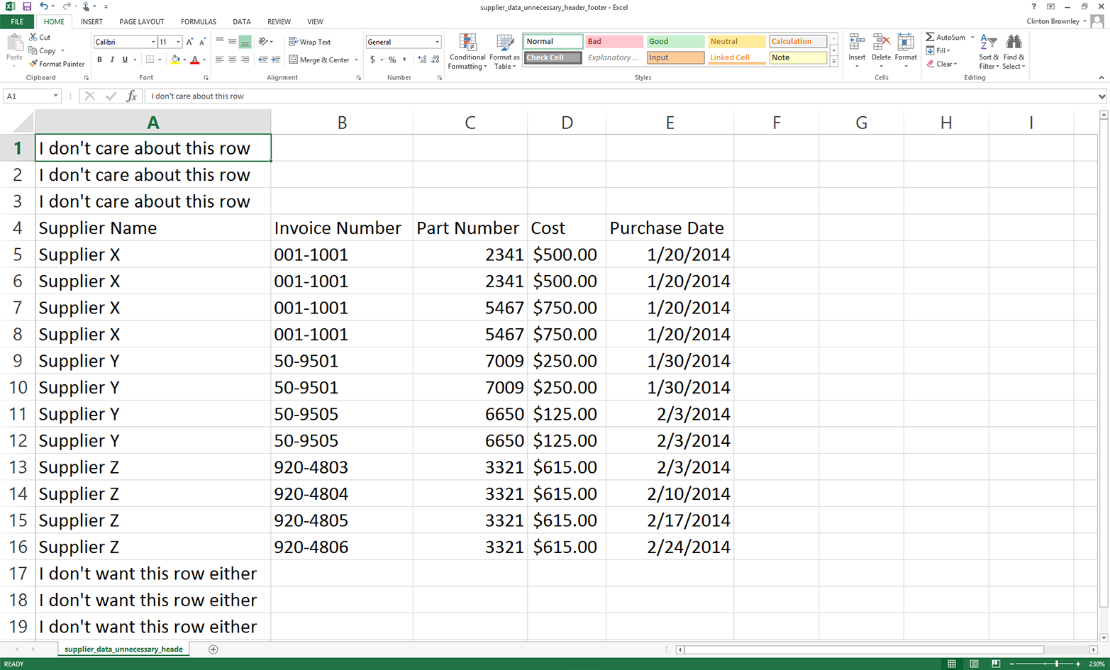
Now that the input file contains unnecessary header and footer information, let’s modify our Python script so that it does not read these lines.
To select specific rows with base Python, we’ll use a row_counter variable to keep track of the row numbers so we can identify and select the rows we want to retain. From the earlier examples, we already know that there are 13 rows of data we want to retain. You can see in the if block shown below that the only rows we want to write to the output file are the ones with row indexes greater than or equal to 3 and less than or equal to 15.
To select these rows with base Python, type the following code into a text editor and save the file as 11csv_reader_select_contiguous_rows.py:
1#!/usr/bin/env python32importcsv3importsys4input_file=sys.argv[1]5output_file=sys.argv[2]6row_counter=07withopen(input_file,'r',newline='')ascsv_in_file:8withopen(output_file,'w',newline='')ascsv_out_file:9filereader=csv.reader(csv_in_file)10filewriter=csv.writer(csv_out_file)11forrowinfilereader:12ifrow_counter>=3androw_counter<=15:13filewriter.writerow([value.strip()forvalueinrow])14row_counter+=115
We use the row_counter variable in combination with an if statement to retain only the rows we care about and skip the unwanted header and footer content. For the first three rows in the input file, row_counter is less than three, so the if block isn’t executed and the value in row_counter increases by one.
For the last three rows in the input file, row_counter is greater than 15, so again the if block isn’t executed and the value in row_counter increases by one.
The rows we want to retain are in between the unnecessary header and footer content. For these rows, row_counter ranges from 3 to 15. The if block processes these rows and writes them to the output file. We use the string module’s strip function in a list comprehension to remove spaces, tabs, and newline characters from both ends of each of the values in each row.
You can see the value of the row_counter variable along with the row content by adding a print statement like print(row_counter, [value.strip() for value in row]) above the existing writerow statement.
To run the script, type the following on the command line and hit Enter:
python 11csv_reader_select_contiguous_rows.py supplier_data_unnecessary_header_\ footer.csv output_files\11output.csv
You can then open the output file, 11output.csv, to review the results.
Pandas provides the drop function for deleting rows or columns based on a row index value or column heading. In the following script, the drop function removes the first three rows and the last three rows from the input file (i.e., the rows whose indexes are 0, 1, and 2 and 16, 17, and 18). Pandas also provides the versatile iloc function, which we can use to select a single row based on its index value to make it the column index. Finally, it provides the reindex function, which we can use to conform one or more axes to new indexes.
To retain the header column row and data rows and remove the unnecessary header and footer rows with pandas, type the following code into a text editor and save the file as pandas_select_contiguous_rows.py:
#!/usr/bin/env python3importpandasaspdimportsysinput_file=sys.argv[1]output_file=sys.argv[2]data_frame=pd.read_csv(input_file,header=None)data_frame=data_frame.drop([0,1,2,16,17,18])data_frame.columns=data_frame.iloc[0]data_frame=data_frame.reindex(data_frame.index.drop(3))data_frame.to_csv(output_file,index=False)
To run the script, type the following on the command line and hit Enter:
python pandas_select_contiguous_rows.py supplier_data_unnecessary_header_\ footer.csv output_files\pandas_output.csv
You can then open the output file, pandas_output.csv, to review the results.
Sometimes a spreadsheet does not contain a header row even though you do want column headings for all of the columns. In this situation, you can add column headings with your script.
To demonstrate how to add column headings in a script, we need to modify our input file:
Open supplier_data.csv in a spreadsheet.
Delete the first row in the file (i.e., the header row that contains the column headings).
Save the file as supplier_data_no_header_row.csv. It should look like Figure 2-11.
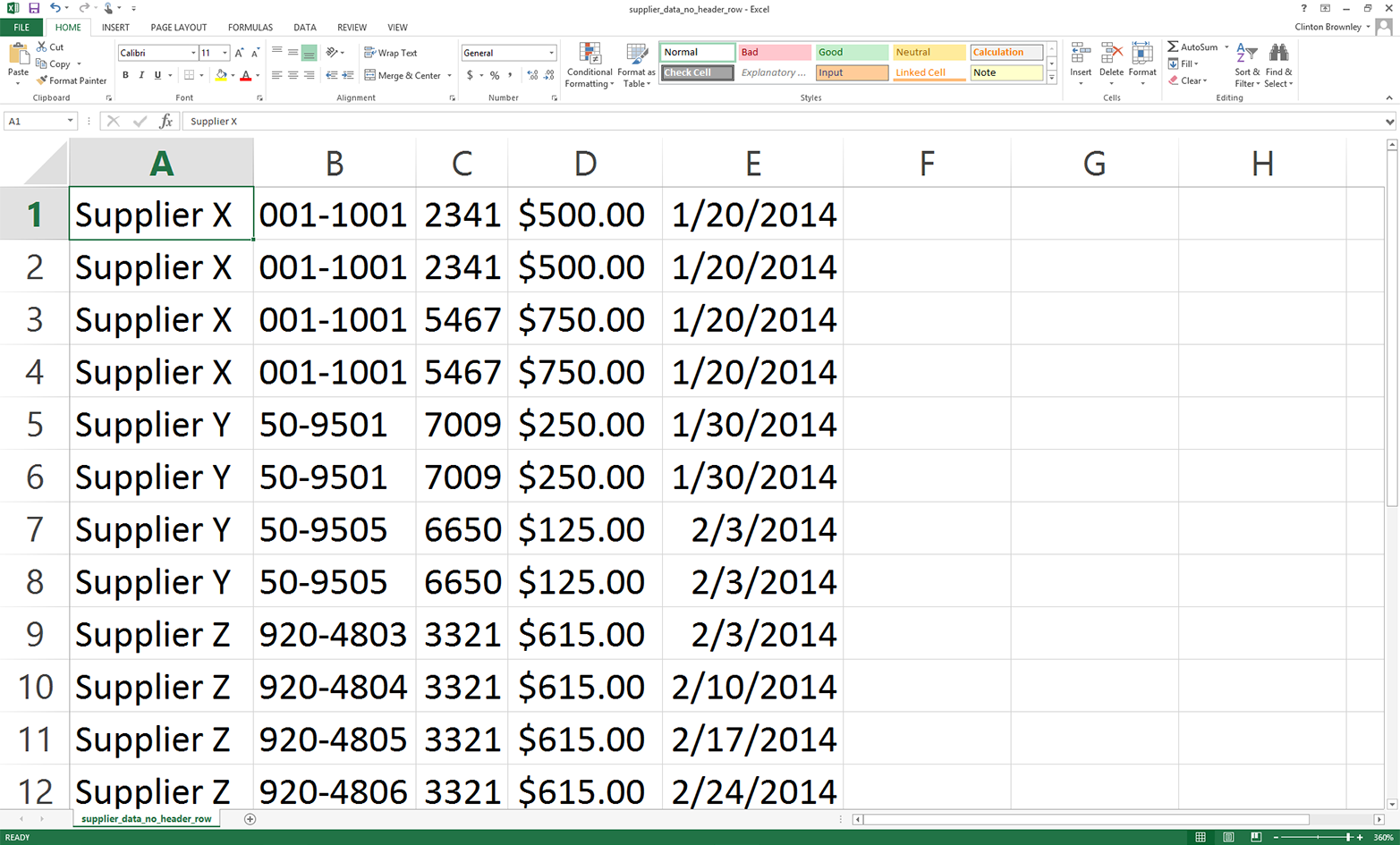
To add column headings in base Python, type the following code into a text editor and save the file as 12csv_reader_add_header_row.py:
1#!/usr/bin/env python32importcsv3importsys4input_file=sys.argv[1]5output_file=sys.argv[2]6withopen(input_file,'r',newline='')ascsv_in_file:7withopen(output_file,'w',newline='')ascsv_out_file:8filereader=csv.reader(csv_in_file)9filewriter=csv.writer(csv_out_file)10header_list=['Supplier Name','Invoice Number',\ 11'Part Number','Cost','Purchase Date']12filewriter.writerow(header_list)13forrowinfilereader:14filewriter.writerow(row)
Line 10 creates a list variable named header_list that contains five string values for the column headings. Line 12 writes the values in this list as the first row in the output file. Similarly, line 14 writes all of the data rows to the output file beneath the header row.
To run the script, type the following on the command line and hit Enter:
python 12csv_reader_add_header_row.py supplier_data_no_header_row.csv\ output_files\12output.csv
You can then open the output file, 12output.csv, to review the results.
The pandas read_csv function makes it straightforward to indicate that the input file doesn’t have a header row and to supply a list of column headings. To add a header row to our dataset that doesn’t have one, type the following code into a text editor and save the file as pandas_add_header_row.py:
#!/usr/bin/env python3importpandasaspdimportsysinput_file=sys.argv[1]output_file=sys.argv[2]header_list=['Supplier Name','Invoice Number',\'Part Number','Cost','Purchase Date']data_frame=pd.read_csv(input_file,header=None,names=header_list)data_frame.to_csv(output_file,index=False)
To run the script, type the following on the command line and hit Enter:
python pandas_add_header_row.py supplier_data_no_header_row.csv\ output_files\pandas_output.csv
You can then open the output file, pandas_output.csv, to review the results.
Up to this point in this chapter, I’ve demonstrated how to process a single CSV file. In some cases, you may only need to process one file. In these cases, the examples thus far should give you an idea of how to use Python to process the file programmatically. Even when you have just one file, the file may be too large to handle manually, and handling it programmatically can also reduce the chances of human errors such as copy/paste errors and typos.
However, in many cases, you need to process lots of files—so many files that it is inefficient or impossible to handle them manually. In these situations, Python is even more exciting because it enables you to automate and scale your data processing above and beyond what you can handle manually. This section introduces Python’s built-in glob module and builds on some of the examples shown earlier in this chapter to demonstrate how to process CSV files at scale.
In order to work with multiple CSV files, we need to create multiple CSV files. We’ll create three files to use in the following examples but remember that the techniques shown here scale to as many files as your computer can handle—hundreds or more!
Open a spreadsheet.
Add the data shown in Figure 2-12.
Save the file as sales_january_2014.csv.
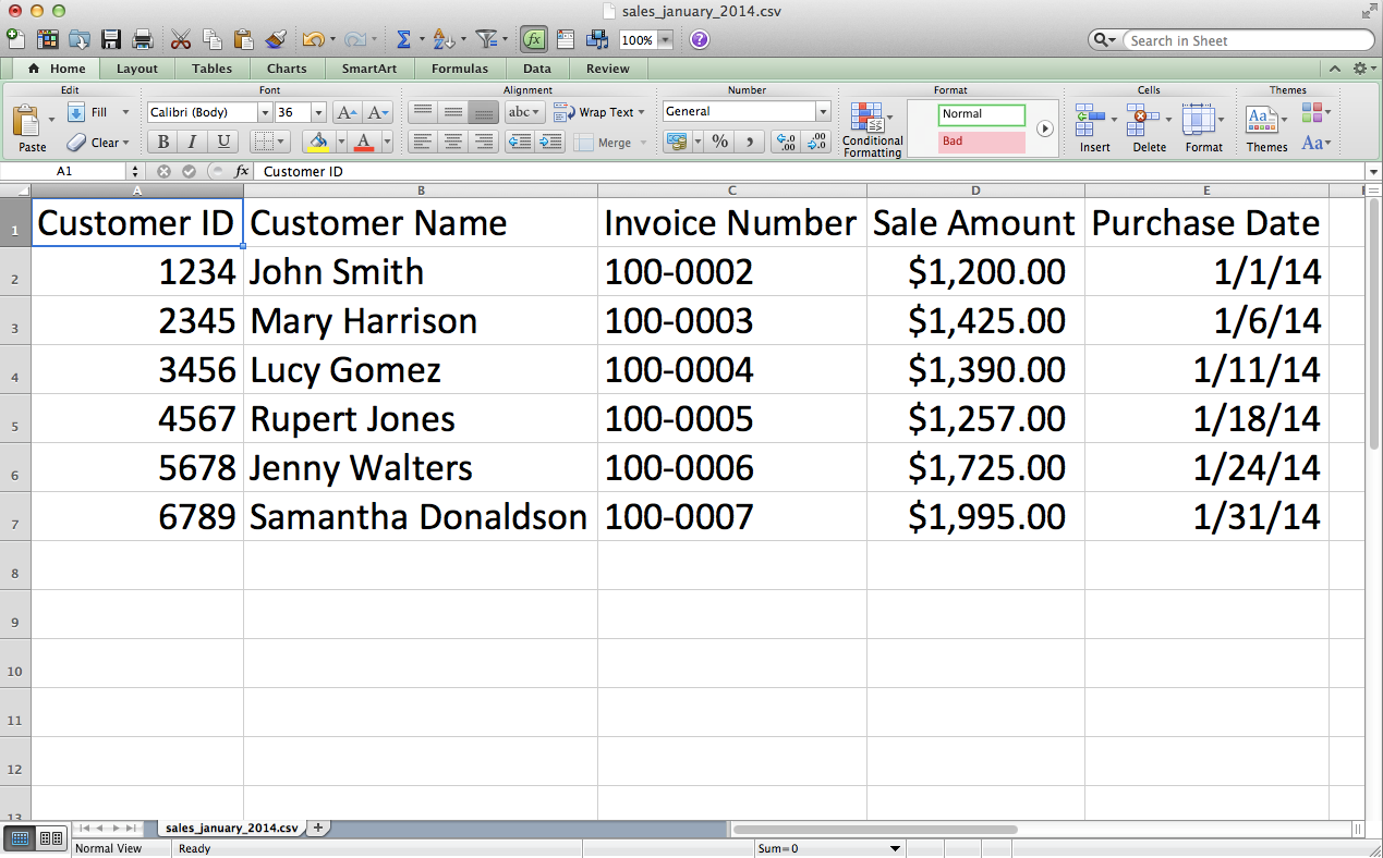
Open a spreadsheet.
Add the data shown in Figure 2-13.
Save the file as sales_february_2014.csv.
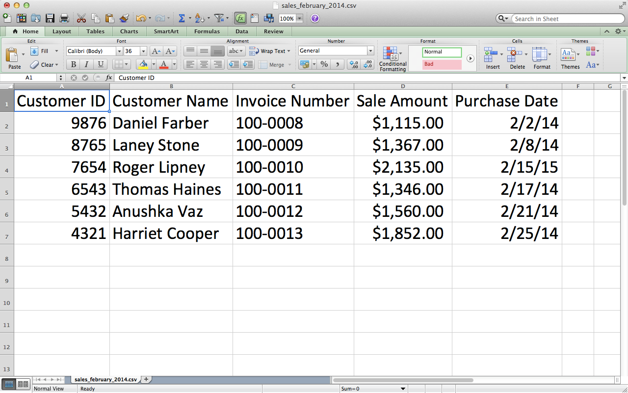
Open a spreadsheet.
Add the data shown in Figure 2-14.
Save the file as sales_march_2014.csv.
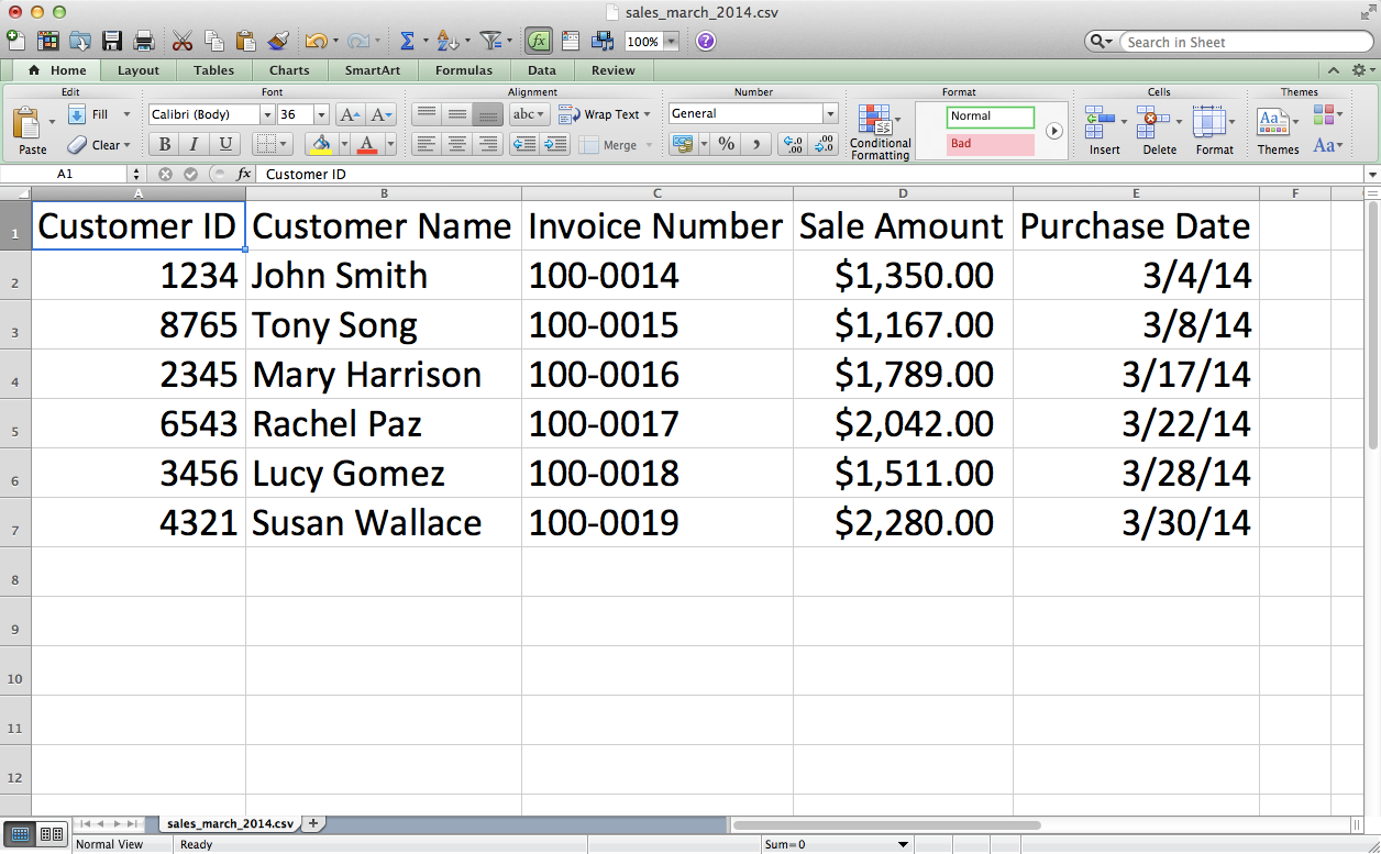
Let’s start with some simple counting of rows and columns; this is pretty basic, but it’s also a good way to get a sense of a new dataset. While in some cases you may know the contents of the input files you’re dealing with, in many cases someone sends you a set of files and you don’t immediately know their contents. In these cases, it’s often helpful to count the number of files you’re dealing with and to count the number of rows and columns in each file.
To process the three CSV files you created in the previous section, type the following code into a text editor and save the file as 8csv_reader_counts_for_multiple_files.py:
1#!/usr/bin/env python32importcsv3importglob4importos5importsys6input_path=sys.argv[1]7file_counter=08forinput_fileinglob.glob(os.path.join(input_path,'sales_*')):9row_counter=110withopen(input_file,'r',newline='')ascsv_in_file:11filereader=csv.reader(csv_in_file)12header=next(filereader,None)13forrowinfilereader:14row_counter+=115('{0!s}:\t{1:d} rows\t{2:d} columns'.format(\ 16os.path.basename(input_file),row_counter,len(header)))17file_counter+=118('Number of files: {0:d}'.format(file_counter))
Lines 3 and 4 import Python’s built-in glob and os modules so we can use their functions to list and parse the pathnames of the files we want to process. The glob module locates all pathnames that match a specific pattern. The pattern can contain Unix shell–style wildcard characters like *. In this specific example, the pattern we’re looking for is 'sales_*'. This pattern means that we’re looking for all files with names that start with sales_ and then have any characters after the underscore. Because you created the three input files, you know that we’re going to use this code to identify our three input files, whose names all start with sales_ and then have different months after the underscore.
In the future, you may want to find all CSV files in a folder, rather than files that start with sales_. If so, then you can simply change the pattern in this script from 'sales_*' to '*.csv'. Because '.csv' is the pattern at the end of all CSV filenames, this pattern effectively finds all CSV files.
The os module contains useful functions for parsing pathnames. For example, os.path.basename(path) returns the basename of path. So, if path is C:\Users\Clinton\Desktop\my_input_file.csv, then os.path.basename(path) returns my_input_file.csv.
Line 8 is the key line for scaling your data processing across multiple input files. Line 8 creates a for loop for iterating through a set of input files and also uses functions from the glob and os modules to create a list of input files to be processed. There is a lot going on in this one line, so let’s review its components from the inside out. The os module’s os.path.join() function joins the two components between the function’s parentheses. input_path is the path to the folder that contains the input files, and 'sales_*' represents any filename that starts with the pattern 'sales_'.
The glob module’s glob.glob() function expands the asterisk (*) in 'sales_*' into the actual filename. In this example, glob.glob() and os.path.join() create a list of our three input files:
['C:\Users\Clinton\Desktop\sales_january_2014.csv', 'C:\Users\Clinton\Desktop\sales_february_2014.csv', 'C:\Users\Clinton\Desktop\sales_march_2014.csv']
Then the for loop syntax at the beginning of the line executes the lines of code indented beneath this line for each of the input files in this list.
Line 15 is a print statement that prints the filename, number of rows in the file, and number of columns in the file for each of the input files. The tab characters, \t, in the print statement are not necessary but help to align the three columns by placing a tab between the columns. This line uses the {} characters to pass these three values into the print statement. For the first value, we use the os.path.basename() function to extract the final element in the full pathname. For the second value, we use a row_counter variable to count the total number of rows in each input file. Finally, for the third value, we use the built-in len function to count the number of values in the list variable header, which contains the list of column headings from each input file. We use this value as the number of columns in each input file. Finally, after line 15 prints information for each file, line 17 uses the value in file_counter to display the number of files the script processed.
To run the script, type the following on the command line and hit Enter:
python 8csv_reader_counts_for_multiple_files.py "C:\Users\Clinton\Desktop"
Notice that the input on the command line after the script name is a path to a folder. In earlier examples, the input in that position was the name of the input file. In this case, we want to process many input files, so we have to point to the folder that holds all of the input files.
You should see the names of the three input files along with the number of rows and columns in each file printed to the screen. Beneath the rows of information about the three input files, the final print statement shows the total number of input files that were processed. The displayed information should look as shown in Figure 2-15.
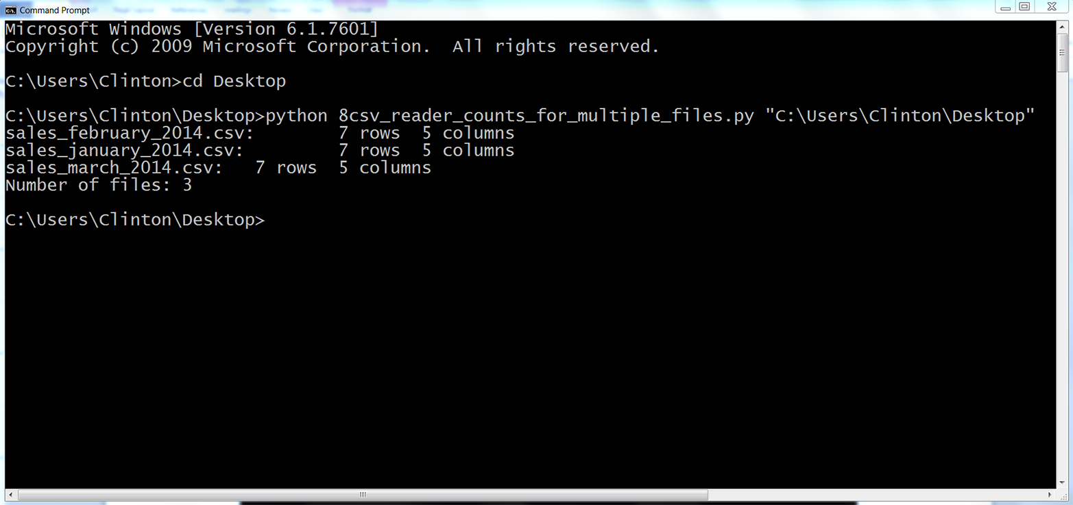
The output shows that the script processed three files and each file has seven rows and five columns.
This example demonstrated how to read multiple CSV files and print some basic information about each of the files to the screen. Printing some basic information about files you plan to process is useful when you’re less familiar with the files you need to process. Understanding the number of input files and the number of rows and columns in each file gives you some idea about the size of the processing job, as well as the potential consistency of the file layouts.
When you have multiple files that contain similar data you’ll often want to concatenate the data so that all of the data is in one file. You may have done this previously by opening each file and copying and pasting the data from each worksheet into a single worksheet. This manual process is time consuming and error prone. Moreover, in some cases, given the quantity and/or size of the files that need to be merged together, a manual process is not even possible.
Given the drawbacks of concatenating data manually, let’s see how to accomplish this task with Python. We’ll use the three CSV files we created at the beginning of this section to demonstrate how to concatenate data from multiple files.
To concatenate data from multiple input files vertically into one output file with base Python, type the following code into a text editor and save the file as 9csv_reader_concat_rows_from_multiple_files.py:
1#!/usr/bin/env python32importcsv3importglob4importos5importsys6input_path=sys.argv[1]7output_file=sys.argv[2]8 9first_file=True10forinput_fileinglob.glob(os.path.join(input_path,'sales_*')):11(os.path.basename(input_file))12withopen(input_file,'r',newline='')ascsv_in_file:13withopen(output_file,'a',newline='')ascsv_out_file:14filereader=csv.reader(csv_in_file)15filewriter=csv.writer(csv_out_file)16iffirst_file:17forrowinfilereader:18filewriter.writerow(row)19first_file=False20else:21header=next(filereader,None)22forrowinfilereader:23filewriter.writerow(row)
Line 13 is a with statement that opens the output file. In earlier examples that involved writing to an output file, the string in the open function has been the letter 'w', meaning the output file has been opened in write mode.
In this example, we use the letter 'a' instead of 'w' to open the output file in append mode. We need to use append mode so that the data from each input file is appended to (i.e., added to) the output file. If we used write mode instead, the data from each input file would overwrite the data from the previously processed input file and the output file would only contain the data from the last input file that was processed.
The if-else statement that starts on line 16 relies on the first_file variable created in line 9 to distinguish between the first input file and all of the subsequent input files. We make this distinction between the input files so that the header row is written to the output file only once. The if block processes the first input file and writes all of the rows, including the header row, to the output file. The else block processes all of the remaining input files and uses the next method to assign the header row in each file to a variable (effectively removing it from further processing) before writing the remaining data rows to the output file.
To run the script, type the following on the command line and hit Enter:
python 9csv_reader_concat_rows_from_multiple_files.py "C:\Users\Clinton\Desktop"\ output_files\9output.csv
You should see the names of the input files printed to the screen, as shown in Figure 2-16.
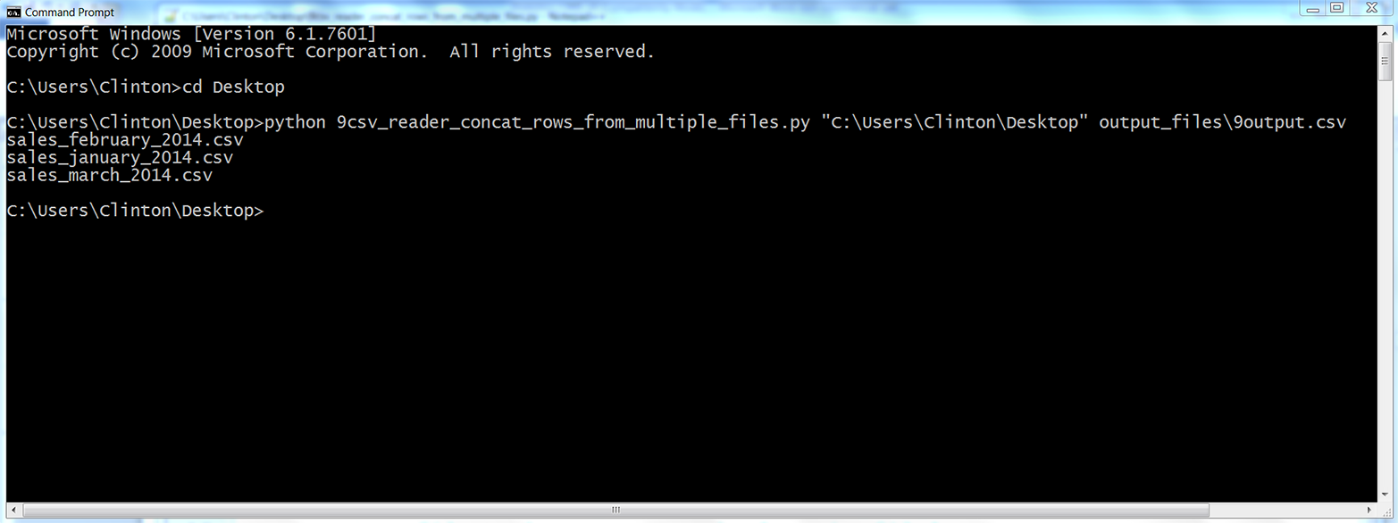
The output on the screen shows the names of the files that were processed. In addition, the script has also concatenated the data from the three input files into a single output file called 9output.csv, located in the output_files folder on your Desktop. Figure 2-17 shows what the contents should look like.
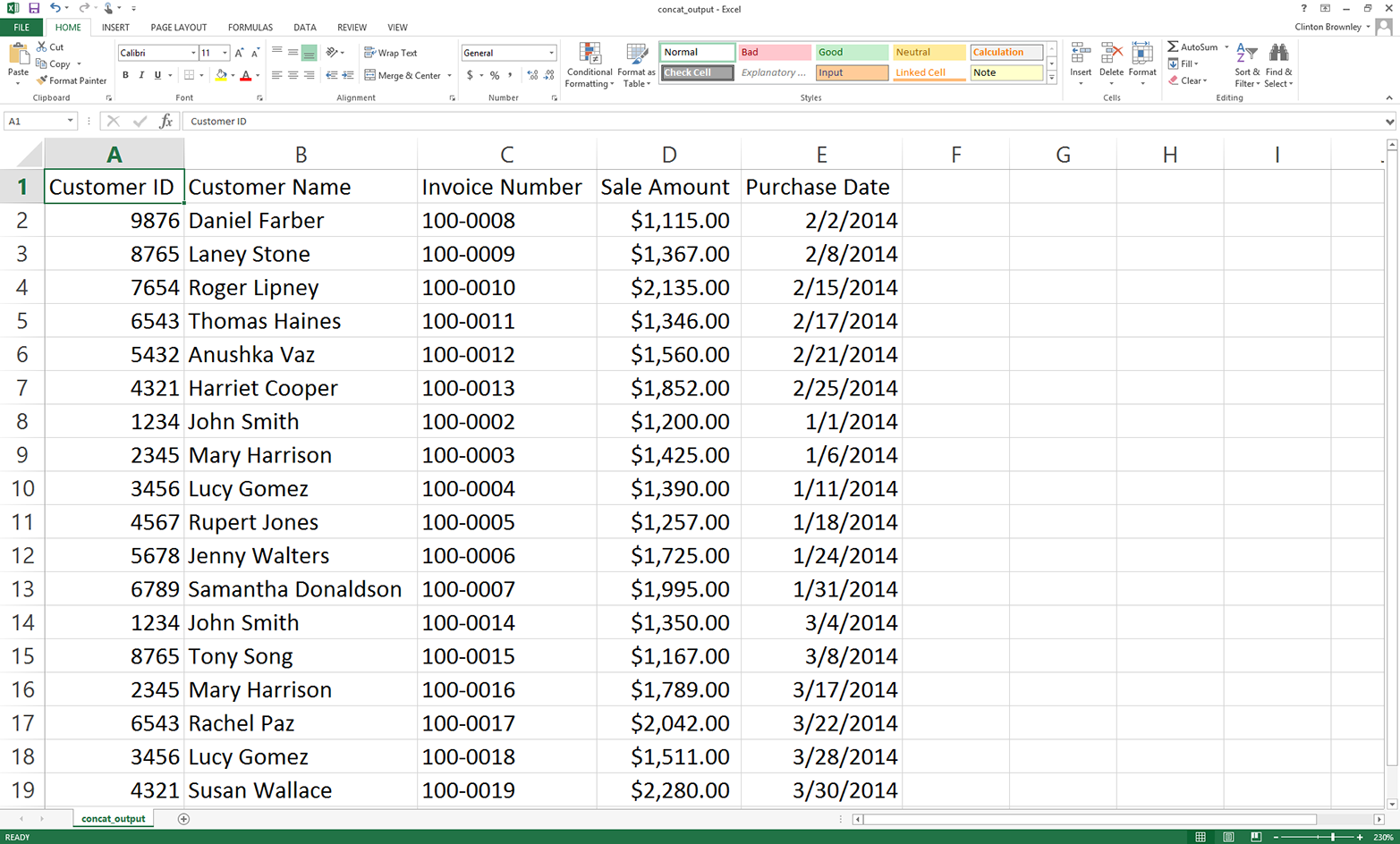
This figure shows that the script successfully concatenated the data from the three input files. The output file contains one header row and all of the data rows from the three input files.
In the code discussion, I mentioned why we use 'a' (append mode) instead of 'w' (write mode) in line 13. I also mentioned why we distinguish between the first input file and all of the subsequent files. To experiment and learn, you may want to change the 'a' to a 'w' and then resave and rerun the script on the input files to see how the output changes. Similarly, you may want to eliminate the if-else statement and simply print all of the rows from all of the input files to see how the output changes.
One important point is that the pattern in this example, 'sales_*', is relatively specific, meaning you’re unlikely to have any files on your Desktop whose names start with ’sales_' besides the three input files. In other situations you’re more likely to use a less specific pattern, like '*.csv' to search for all CSV files. In these situations, you don’t want to create your output file in the same folder that contains all of your input files. The reason you don’t want to do this is that, in the script, you open the output file while you’re still processing input files. So, if your pattern is '*.csv' and your output file is a CSV file, then your script is going to try to process the output file like one of your input files, which is going to cause problems and errors. This possibility is why it is better practice to send an output file to a different folder, as we did in this example.
Pandas makes it straightforward to concatenate data from multiple files. The basic process is to read each input file into a pandas DataFrame, append all of the DataFrames into a list of DataFrames, and then use the concat function to concatenate all of the DataFrames together into one DataFrame. The concat function has an axis argument you can use to specify that you want to stack the DataFrames vertically on top of one another (axis=0) or horizontally side by side (axis=1).
To concatenate data from multiple input files vertically into one output file with pandas, type the following code into a text editor and save the file as pandas_concat_rows_from_multiple_files.py:
#!/usr/bin/env python3importpandasaspdimportglobimportosimportsysinput_path=sys.argv[1]output_file=sys.argv[2]all_files=glob.glob(os.path.join(input_path,'sales_*'))all_data_frames=[]forfileinall_files:data_frame=pd.read_csv(file,index_col=None)all_data_frames.append(data_frame)data_frame_concat=pd.concat(all_data_frames,axis=0,ignore_index=True)data_frame_concat.to_csv(output_file,index=False)
This code stacks the DataFrames vertically. If instead you need to concatenate them horizontally, then set axis=1 in the concat function. In addition to a DataFrame, pandas also has a Series data container. You use identical syntax to concatenate Series, except the objects you concatenate are Series instead of DataFrames.
Sometimes, instead of simply concatenating the data vertically or horizontally, you need to join the datasets together based on the values in a key column in the datasets. Pandas offers a merge function that provides these SQL join–like operations. If you’re familiar with SQL joins, then it’ll be easy for you to pick up the merge function’s syntax: pd.merge(DataFrame1, DataFrame2, on='key', how='inner').
NumPy, another add-in Python module, also provides several functions for concatenating data vertically and horizontally. It’s conventional to import NumPy as np. Then, to concatenate data vertically, you can use np.concatenate([array1, array2], axis=0), np.vstack((array1, array2)), or np.r_[array1, array2]. Similarly, to concatenate data horizontally, you can use np.concatenate([array1, array2], axis=1), np.hstack((array1, array2)), or np.c_[array1, array2].
To run the script, type the following on the command line and hit Enter:
python pandas_concat_rows_from_multiple_files.py "C:\Users\Clinton\Desktop"\ output_files\pandas_output.csv
You can then open the output file, pandas_output.csv, to review the results.
Sometimes when you have multiple input files, you need to calculate a few statistics for each input file. The example in this section uses the three CSV files we created earlier and shows how to calculate a column sum and average for each input file.
To calculate a column sum and average for multiple files with base Python, type the following code into a text editor and save the file as 10csv_reader_sum_average_from_multiple_files:
1#!/usr/bin/env python32importcsv3importglob4importos5importsys6input_path=sys.argv[1]7output_file=sys.argv[2]8output_header_list=['file_name','total_sales','average_sales']9csv_out_file=open(output_file,'a',newline='')10filewriter=csv.writer(csv_out_file)11filewriter.writerow(output_header_list)12forinput_fileinglob.glob(os.path.join(input_path,'sales_*')):13withopen(input_file,'r',newline='')ascsv_in_file:14filereader=csv.reader(csv_in_file)15output_list=[]16output_list.append(os.path.basename(input_file))17header=next(filereader)18total_sales=0.019number_of_sales=0.020forrowinfilereader:21sale_amount=row[3]22total_sales+=float(str(sale_amount).strip('$').replace(',',''))23number_of_sales+=124average_sales='{0:.2f}'.format(total_sales/number_of_sales)25output_list.append(total_sales)26output_list.append(average_sales)27filewriter.writerow(output_list)28csv_out_file.close()
Line 8 creates a list of the column headings for the output file. Line 10 creates the filewriter object, and line 11 writes the header row to the output file.
Line 15 creates an empty list that will store each row of output that we’ll write to the output file. Because we want to calculate a sum and an average for each input file, line 16 appends the name of the input file into the output_list.
Line 17 uses the next function to remove the header row from each input file. Line 18 creates a variable named total_sales and sets its value equal to zero. Similarly, line 19 creates a variable named number_of_sales and sets its value equal to zero. Line 20 is a for loop for iterating over the data rows in each of the input files.
Line 21 uses list indexing to extract the value in the Sale Amount column and assigns it to the variable named sale_amount. Line 22 uses the str function to ensure the value in sale_amount is a string and then uses the strip and replace functions to remove any dollar signs and commas in the value. Then it uses the float function to convert the value to a floating-point number, and adds the value to the value in total_sales. Line 23 adds one to the value in number_of_sales.
Line 24 divides the value in total_sales by the value in number_of_sales to calculate the average sales for the input file and assigns this number, formatted to two decimal places and converted into a string, to the variable average_sales.
Line 25 adds the total sales as the second value in output_list. The first value in the list is the name of the input file. This value is added to the list in line 17. Line 26 adds the average sales as the third value in output_list. Line 27 writes the values in output_list to the output file.
The script executes this code for each of the input files, so the output file will contain a column of filenames, a column of total sales, and a column of average sales corresponding to each of the input files.
To run the script, type the following on the command line and hit Enter:
python 10csv_reader_sum_average_from_multiple_files.py \ "C:\Users\Clinton\Desktop" output_files\10output.csv
You can then open the output file, 10output.csv, to review the results.
Pandas provides summary statistics functions, like sum and mean, that you can use to calculate row and column statistics. The following code demonstrates how to calculate two statistics (sum and mean) for a specific column in multiple input files and write the results for each input file to an output file.
To calculate these two column statistics with pandas, type the following code into a text editor and save the file as pandas_ sum_average_from_multiple_files.py:
#!/usr/bin/env python3importpandasaspdimportglobimportosimportsysinput_path=sys.argv[1]output_file=sys.argv[2]all_files=glob.glob(os.path.join(input_path,'sales_*'))all_data_frames=[]forinput_fileinall_files:data_frame=pd.read_csv(input_file,index_col=None)total_sales=pd.DataFrame([float(str(value).strip('$').replace(',',''))\forvalueindata_frame.loc[:,'Sale Amount']]).sum()average_sales=pd.DataFrame([float(str(value).strip('$').replace(',',''))\forvalueindata_frame.loc[:,'Sale Amount']]).mean()data={'file_name':os.path.basename(input_file),'total_sales':total_sales,'average_sales':average_sales}all_data_frames.append(pd.DataFrame(data,\columns=['file_name','total_sales','average_sales']))data_frames_concat=pd.concat(all_data_frames,axis=0,ignore_index=True)data_frames_concat.to_csv(output_file,index=False)
We use list comprehensions to convert the string dollar values in the Sale Amount column into floating-point numbers, and then we use the DataFrame function to convert the object into a DataFrame so we can use the two functions to calculate the sum and mean values for the column.
Because each row in the output file should contain the input filename, sum, and mean for the Sale Amount column in the file, we combine these three pieces of data into a DataFrame, use the concat function to concatenate all of the DataFrames together into one DataFrame, and then write the DataFrame to an output file.
To run the script, type the following on the command line and hit Enter:
python pandas_ sum_average_from_multiple_files.py "C:\Users\Clinton\Desktop"\ output_files\pandas_output.csv
You can then open the output file, pandas_output.csv, to review the results.
We’ve covered a lot of ground in this chapter. We’ve discussed how to read and parse a CSV file, navigate rows and columns in a CSV file, process multiple CSV files, and calculate statistics for multiple CSV files. If you’ve followed along with the examples in this chapter, you have written 12 Python scripts.
The best part about all of the work you have put into working through the examples in this chapter is that they are the basic building blocks for navigating and processing files. Having gone through the examples in this chapter, you’re now well prepared to process Excel files, the topic of our next chapter.
Modify one of the scripts that filters for rows based on conditions, sets, or regular expressions to print and write a different set of rows than the ones we filtered for in the examples.
Modify one of the scripts that filters for columns based on index values or column headings to print and write a different set of columns than the ones we filtered for in the examples.
Create a new set of CSV input files in a folder, create a separate output folder, and use one of the scripts that processes multiple files to process the new input files and write the results to the output folder.
Microsoft Excel is ubiquitous. We use Excel to store data on customers, inventory, and employees. We use it to track operations, sales, and financials. The list of ways people use Excel in business is long and diverse. Because Excel is such an integral tool in business, knowing how to process Excel files in Python will enable you to add Python into your data processing workflows, receiving data from other people and sharing results with them in ways they’re comfortable with.
Unlike Python’s csv module, there is not a standard module in Python for processing Excel files (i.e., files with the .xls or .xlsx extension). To complete the examples in this section, you need to have the xlrd and xlwt packages. The xlrd and xlwt packages enable Python to process Excel files on any operating system, and they have strong support for Excel dates. If you installed Anaconda Python, then you already have the packages because they’re bundled into the installation. If you installed Python from the Python.org website, then you need to follow the instructions in Appendix A to download and install the two packages.
A few words on terminology: when I refer to an “Excel file” that’s the same thing as an “Excel workbook.” An Excel workbook contains one or more Excel worksheets. In this chapter, I’ll be using the words “file” and “workbook” interchangeably, and I’ll refer to the individual worksheets within a workbook as worksheets.
As we did when working with CSV files in Chapter 2, we’ll go through each of the examples here in base Python, so you can see every logical step in the data processing, and then using pandas, so you can have a (usually) shorter and more concise example—though one that’s a bit more abstract—if you want to copy and modify it for use in your work.
To get started with the examples in this chapter, we need to create an Excel workbook:
Open Microsoft Excel.
Add three separate worksheets to the workbook and name them january_2013, february_2013, and march_2013. Then add the data as shown in Figure 3-1, Figure 3-2, and Figure 3-3, respectively.
Save the workbook as sales_2013.xlsx.
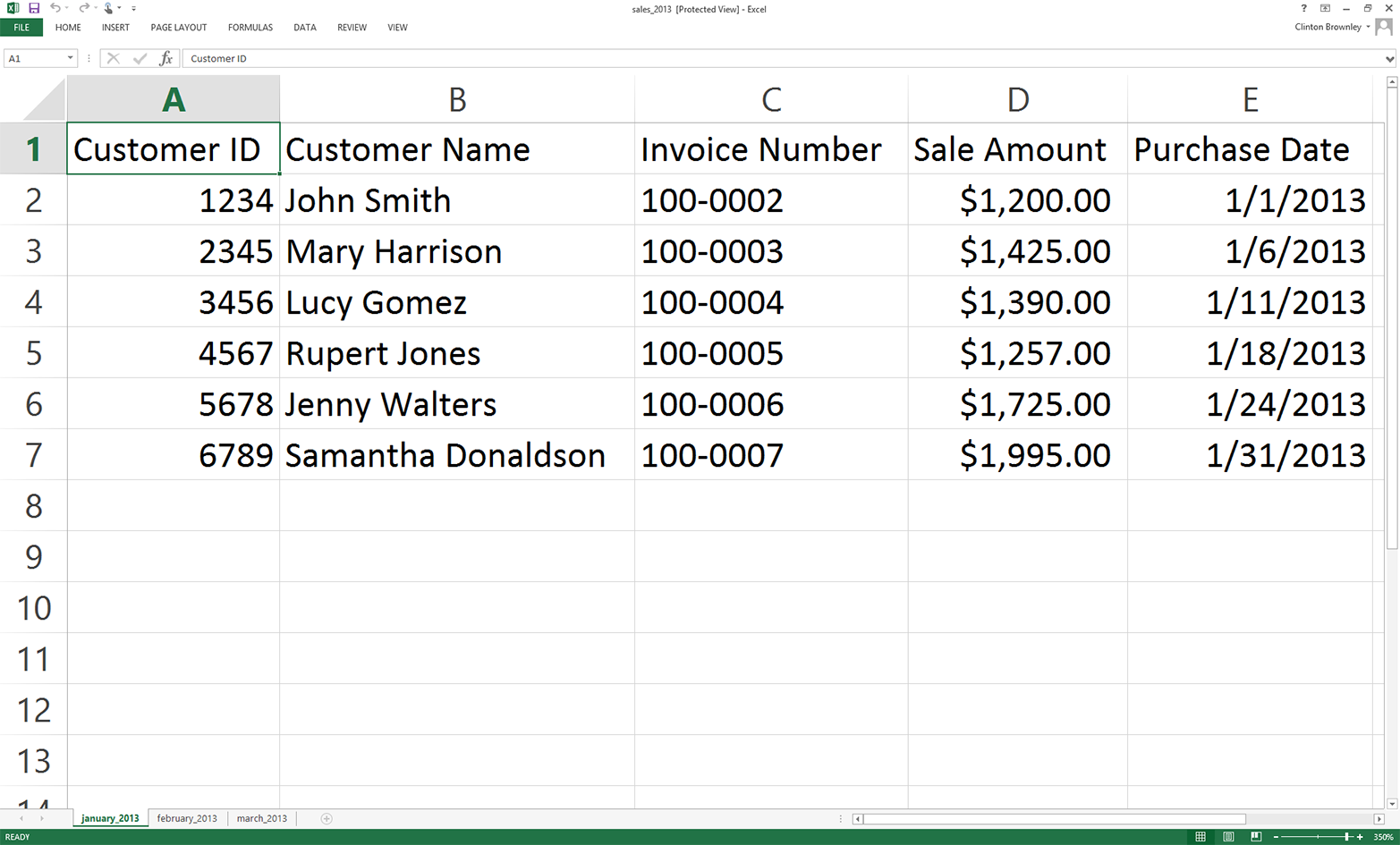
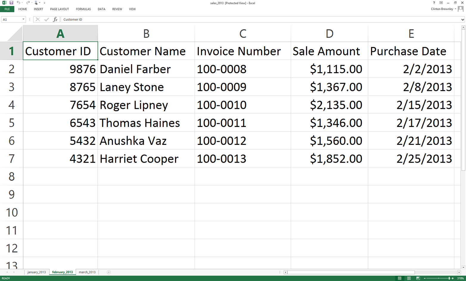
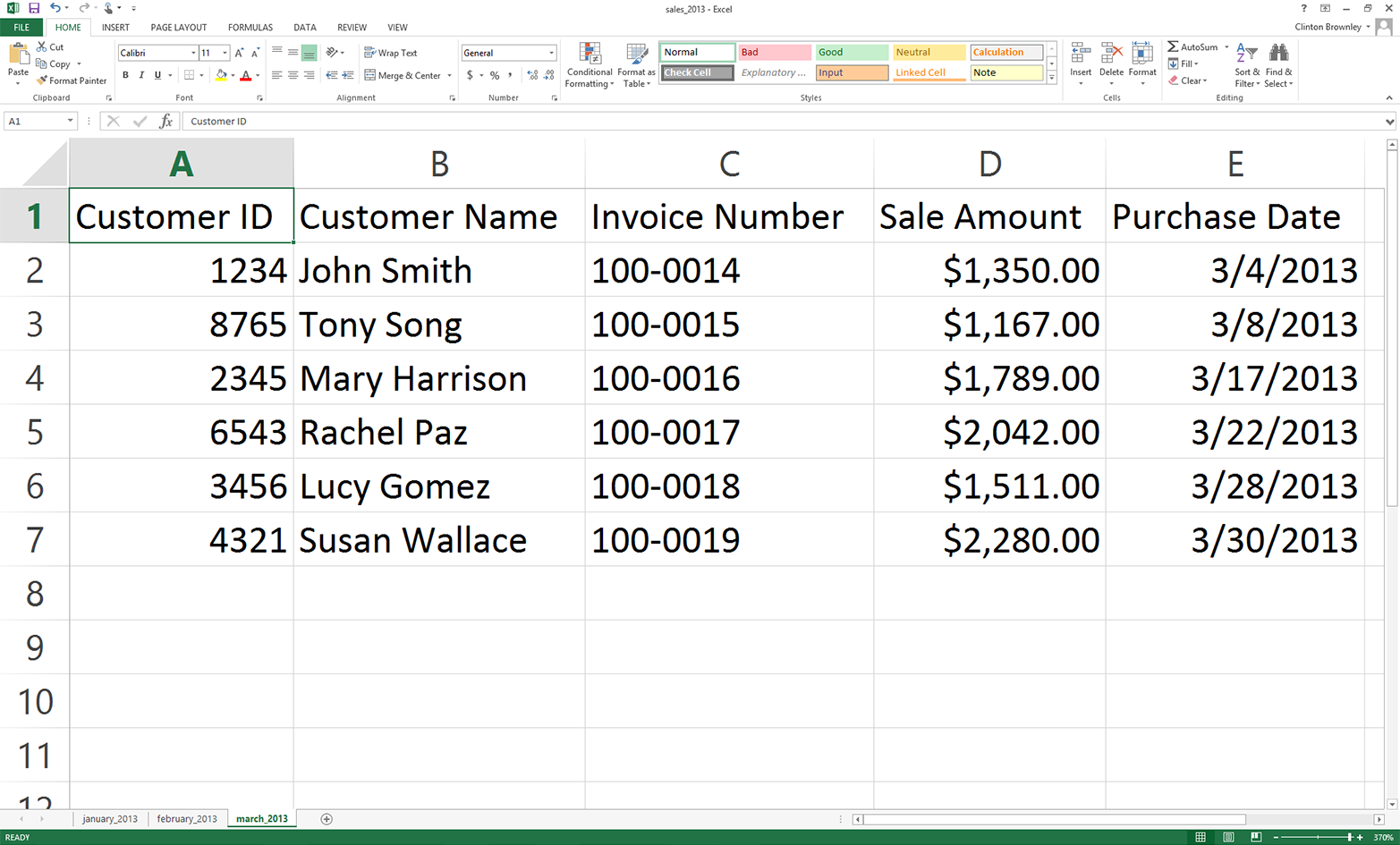
Now that we have an Excel workbook that contains three worksheets, let’s learn how to process an Excel workbook in Python. As a reminder, we are using the xlrd and xlwt packages in this chapter, so make sure you have already downloaded and installed these add-in packages.
As you are probably already aware, Excel files are different from CSV files in at least two important respects. First, unlike a CSV file, an Excel file is not a plain-text file, so you cannot open it and view the data in a text editor. You can see this by right-clicking on the Excel workbook you just created and opening it in a text editor like Notepad or TextWrangler. Instead of legible data, you will see a mess of special characters.
Second, unlike a CSV file, an Excel workbook is designed to contain multiple worksheets. Because a single Excel workbook can contain multiple worksheets, we need to learn how to introspect (i.e., look inside and examine) all of the worksheets in a workbook without having to manually open the workbook. By introspecting a workbook, we can examine the number of worksheets and the types and amount of data on each worksheet before we actually process the data in the workbook.
Introspecting Excel files is useful to make sure that they contain the data you expect, and to do a quick check for consistency and completeness. That is, understanding the number of input files and the number of rows and columns in each file will give you some idea about the size of the processing job as well as the potential consistency of the file layouts.
Once you understand how to introspect the worksheets in a workbook, we will move on to parsing a single worksheet, iterating over multiple worksheets, and then iterating over multiple workbooks.
To determine the number of worksheets in the workbook, the names of the worksheets, and the number of rows and columns in each of the worksheets, type the following code into a text editor and save the file as 1excel_introspect_workbook.py:
1#!/usr/bin/env python32importsys3fromxlrdimportopen_workbook4input_file=sys.argv[1]5workbook=open_workbook(input_file)6('Number of worksheets:',workbook.nsheets)7forworksheetinworkbook.sheets():8("Worksheet name:",worksheet.name,"\tRows:",\ 9worksheet.nrows,"\tColumns:",worksheet.ncols)
Figure 3-4, Figure 3-5, and Figure 3-6 show what the script looks like in Anaconda Spyder, Notepad++ (Windows), and TextWrangler (macOS), respectively.
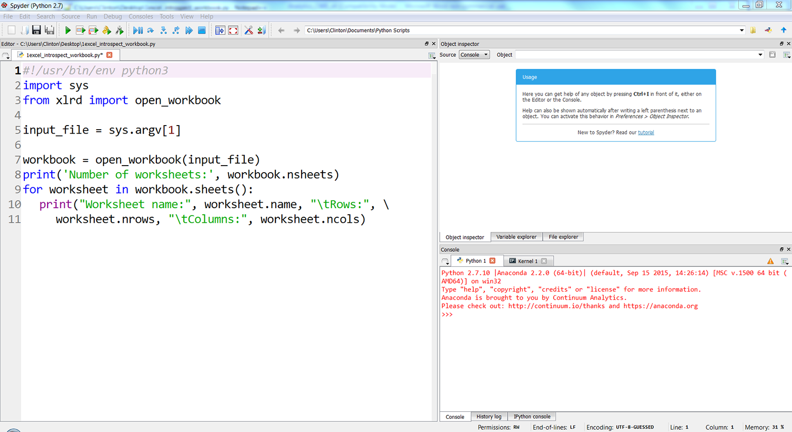
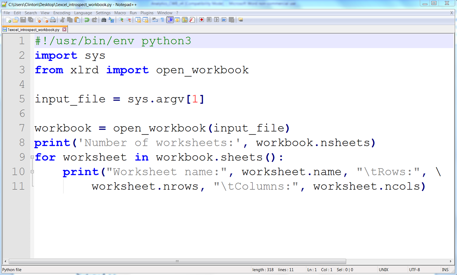
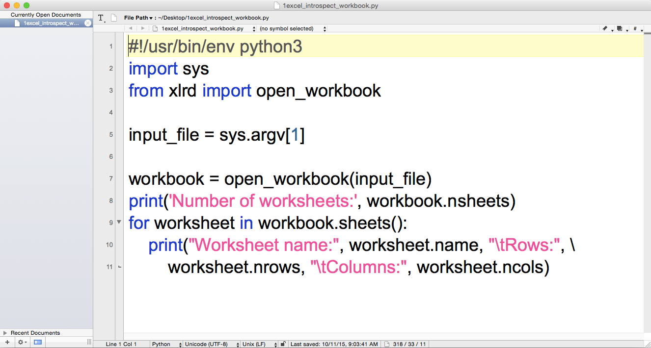
Line 3 imports the xlrd module’s open_workbook function so we can use it to read and parse an Excel file.
Line 7 uses the open_workbook function to open the Excel input file into an object I’ve named workbook. The workbook object contains all of the available information about the workbook, so we can use it to retrieve individual worksheets from the workbook.
Line 8 prints the number of worksheets in the workbook.
Line 9 is a for loop that iterates over all of the worksheets in the workbook. The workbook object’s sheets method identifies all of the worksheets in the workbook.
Line 10 prints the name of each worksheet and the number of rows and columns in each worksheet to the screen. The print statement uses the worksheet object’s name attribute to identify the name of each worksheet. Similarly, it uses the nrows and ncols attributes to identify the number of rows and columns, respectively, in each worksheet.
If you created the file in the Spyder IDE, then to run the script:
Click on the Run drop-down menu in the upper-left corner of the IDE.
Select “Configure”
After the Run Settings window opens, select the “Command line options” check box and enter “sales_2013.xlsx” (see Figure 3-7).
Make sure the “Working directory” is where you saved the script and Excel file.
Click Run.
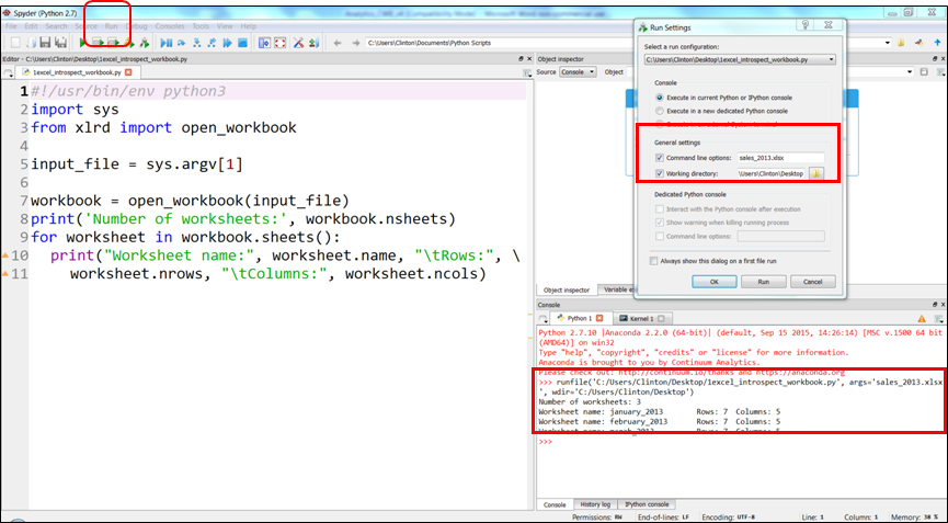
When you click the Run button (either the Run button in the Run Settings window or the green Run button in the upper-left corner of the IDE) you’ll see the output displayed in the Python console in the lower righthand pane of the IDE. Figure 3-7 displays the Run drop-down menu, the key settings in the Run Settings window, and the output inside red boxes.
Alternatively, you can run the script in a Command Prompt or Terminal window. To do so, use one of the following commands, depending on your operating system.
On Windows:
python 1excel_introspect_workbook.py sales_2013.xlsx
On macOS:
chmod +x 1excel_introspect_workbook.py ./1excel_introspect_workbook.py sales_2013.xlsx
You should see the output shown in Figure 3-8 (for Windows) or Figure 3-9 (for macOS) printed to the screen.
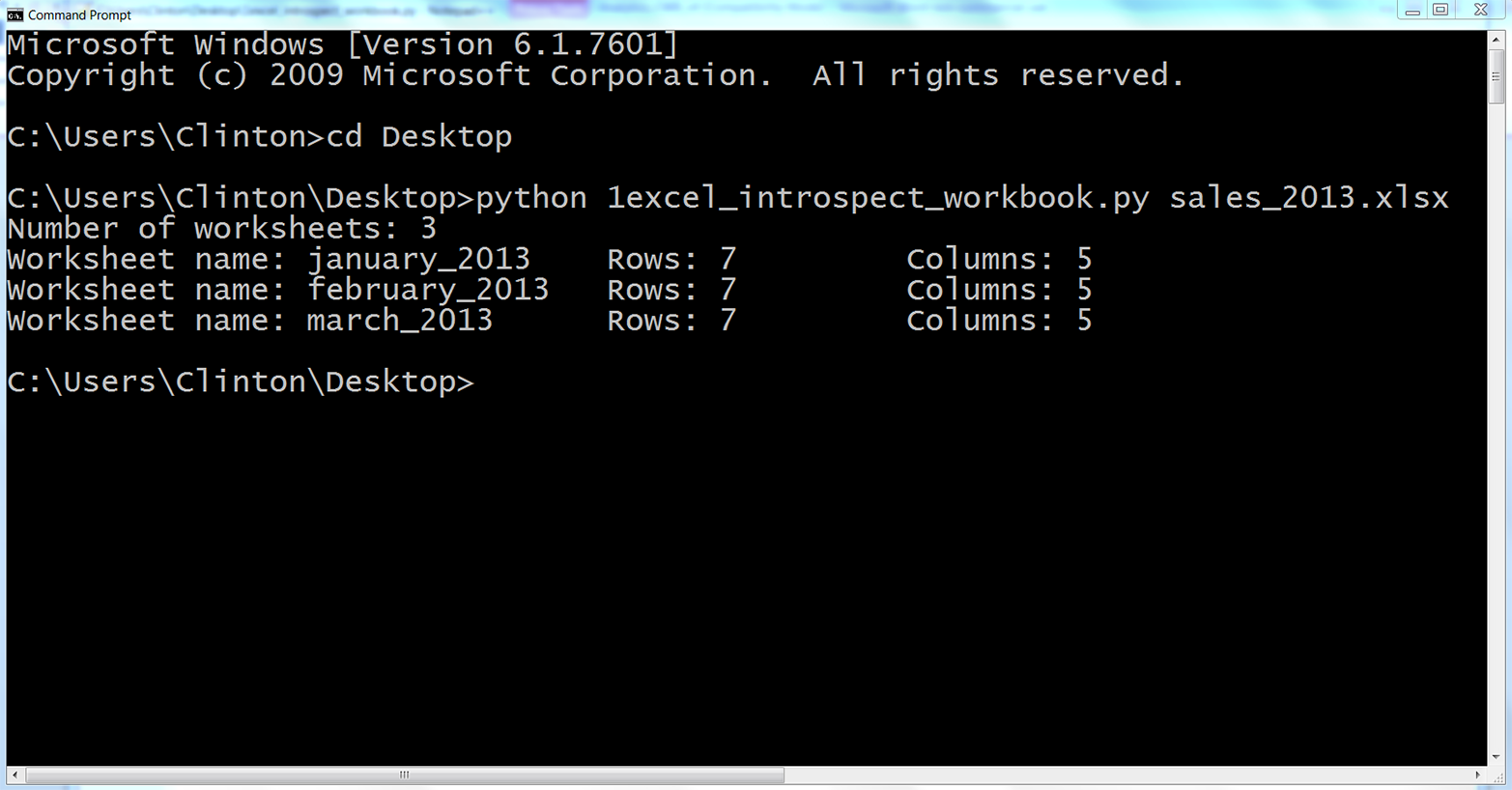
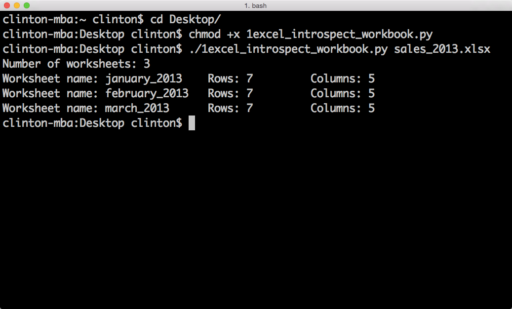
The first line of output shows that the Excel input file, sales_2013.xlsx, contains three worksheets. The next three lines show that the three worksheets are named january_2013, february_2013, and march_2013. They also show that each of the worksheets contains seven rows, including the header row, and five columns.
Now that we know how to use Python to introspect an Excel workbook, let’s learn how to parse a single worksheet in different ways. We’ll then extend that knowledge to iterate over multiple worksheets and then to iterate over multiple workbooks.
While Excel workbooks can contain multiple worksheets, sometimes you only need data from one of the worksheets. In addition, once you know how to parse one worksheet, it is a simple extension to parse multiple worksheets.
To read and write an Excel file with base Python and the xlrd and xlwt modules, type the following code into a text editor and save the file as 2excel_parsing_and_write.py:
1#!/usr/bin/env python32importsys3fromxlrdimportopen_workbook4fromxlwtimportWorkbook5input_file=sys.argv[1]6output_file=sys.argv[2]7output_workbook=Workbook()8output_worksheet=output_workbook.add_sheet('jan_2013_output')9withopen_workbook(input_file)asworkbook:10worksheet=workbook.sheet_by_name('january_2013')11forrow_indexinrange(worksheet.nrows):12forcolumn_indexinrange(worksheet.ncols):13output_worksheet.write(row_index,column_index,\ 14worksheet.cell_value(row_index,column_index))15output_workbook.save(output_file)
Line 3 imports xlrd’s open_workbook function and line 4 imports xlwt’s Workbook object.
Line 7 instantiates an xlwt Workbook object so we can write the results to an output Excel workbook. Line 8 uses xlwt’s add_sheet function to add a worksheet named jan_2013_output inside the output workbook.
Line 9 uses xlrd’s open_workbook function to open the input workbook into a workbook object. Line 10 uses the workbook object’s sheet_by_name function to access the worksheet titled january_2013.
Lines 11 and 12 create for loops over the row and column index values, using the range function and the worksheet object’s nrows and ncols attributes, so we can iterate through each of the rows and columns in the worksheet.
Line 13 uses xlwt’s write function and row and column indexes to write every cell value to the worksheet in the output file.
Finally, line 15 saves and closes the output workbook.
To run the script, type the following on the command line and hit Enter:
python 2excel_parsing_and_write.py sales_2013.xlsx output_files\2output.xls
You can then open the output file, 2output.xls, to review the results.
You may have noticed that the dates in the Purchase Date column, column E, appear to be numbers instead of dates. Excel stores dates and times as floating-point numbers representing the number of days since 1900-Jan-0, plus a fractional portion of a 24-hour day. For example, the number 1 represents 1900-Jan-1, as one day has passed since 1900-Jan-0. Therefore, the numbers in this column represent dates, but they are not formatted as dates.
The xlrd package provides additional functions for formatting date-like values. The next example augments the previous example by demonstrating how to format date-like values so date-like values printed to the screen and written to the output file appear as they do in the input file.
This example builds on the previous example by showing how to use xlrd to maintain date formats as they appear in input Excel files. For example, if a date in an Excel worksheet is 1/19/2000, then we usually want to write 1/19/2000 or another related date format to the output file. However, as the previous example showed, with our current code, we will end up with the number 36544.0 in the output file, as that is the number of days between 1/0/1900 and 1/19/2000.
To apply formatting to our date column, type the following code into a text editor and save the file as 3excel_parsing_and_write_keep_dates.py:
1#!/usr/bin/env python32importsys3fromdatetimeimportdate4fromxlrdimportopen_workbook,xldate_as_tuple5fromxlwtimportWorkbook6input_file=sys.argv[1]7output_file=sys.argv[2]8output_workbook=Workbook()9output_worksheet=output_workbook.add_sheet('jan_2013_output')10withopen_workbook(input_file)asworkbook:11worksheet=workbook.sheet_by_name('january_2013')12forrow_indexinrange(worksheet.nrows):13row_list_output=[]14forcol_indexinrange(worksheet.ncols):15ifworksheet.cell_type(row_index,col_index)==3:16date_cell=xldate_as_tuple(worksheet.cell_value\ 17(row_index,col_index),workbook.datemode)18date_cell=date(*date_cell[0:3]).strftime\ 19('%m/%d/%Y')20row_list_output.append(date_cell)21output_worksheet.write(row_index,col_index,date_cell)22else:23non_date_cell=worksheet.cell_value\ 24(row_index,col_index)25row_list_output.append(non_date_cell)26output_worksheet.write(row_index,col_index,\ 27non_date_cell)28output_workbook.save(output_file)
Line 3 imports the date function from the datetime module so we can cast values as dates and format the dates.
Line 4 imports two functions from the xlrd module. We used the first function to open an Excel workbook in the previous example, so I’ll focus on the second function. The xldate_as_tuple function enables us to convert Excel numbers that are presumed to represent dates, times, or date-times into tuples. Once we convert the numbers into tuples, we can extract specific date elements (e.g., year, month, and day) and format the elements into different date formats (e.g., 1/1/2010 or January 1, 2010).
Line 15 creates an if-else statement to test whether the cell type is the number three. If you review the xlrd module’s documentation, you’ll see that cell type three means the cell contains a date. Therefore, the if-else statement tests whether each cell it sees contains a date. If it does, then the code in the if block operates on the cell; if it doesn’t, then the code in the else block operates on the cell. Because the dates are in the last column, the if block handles the last column.
Line 18 uses the worksheet object’s cell_value function and row and column indexing to access the value in the cell. Alternatively, you could use the cell().value function; both versions give you the same results. This cell value is then the first argument in the xldate_as_tuple function, which converts the floating-point number into a tuple that represents the date.
The workbook.datemode argument is required so that the function can determine whether the date is 1900-based or 1904-based and therefore convert the number to the correct tuple (some versions of Excel for Mac calculate dates from January 1, 1904; for more information on this, read the Microsoft reference guide). The result of the xldate_as_tuple function is assigned to a tuple variable called date_cell. This line is so long that it’s split over two lines in the text, with a backslash as the last character of the first line (you’ll remember from Chapter 1 that the backslash is required so Python interprets the two lines as one line). However, in your script, all of the code can appear on one line without the backslash.
Line 18 uses tuple indexing to access the first three elements in the date_cell tuple (i.e., the year, month, and day elements) and pass them as arguments to the date function, which converts the values into a date object as discussed in Chapter 1. Next, the strftime function converts the date object into a string with the specified date format. The format, '%m/%d/%Y', specifies that a date like March 15, 2014 should appear as 03/15/2014. The formatted date string is reassigned to the variable called date_cell. Line 20 uses the list’s append function to append the value in date_cell into the output list called row_list_output.
To get a feel for the operations taking place in lines 16 and 18, after running the script as is, add a print statement (i.e., print(date_cell)) between the two date_cell = ... lines. Resave and rerun the script to see the result of the xldate_as_tuple function printed to the screen. Next, remove that print statement and move it beneath the second date_cell = ... line. Resave and rerun the script to see the result of the date.strftime functions printed to the screen. These print statements help you see how the functions in these two lines convert the number representing a date in Excel into a tuple and then into a text string formatted as a date.
The else block operates on all of the non-date cells. Line 23 uses the worksheet object’s cell_value function and row and column indexing to access the value in the cell and assigns it to a variable called non_date_cell. Line 25 uses the list’s append function to append the value in non_date_cell into row_list_output. Together, these two lines extract the values in the first four columns of each row as is and append them into row_list_output.
After all of the columns in the row have been processed and added to row_list_output, line 26 writes the values in row_list_output to the output file.
To run the script, type the following on the command line and hit Enter:
python 3excel_parsing_and_write_keep_dates.py sales_2013.xlsx\ output_files\3output.xls
You can then open the output file, 3output.xls, to review the results.
Pandas has a set of commands for reading and writing Excel files as well. Here is a code example that will use pandas for Excel file parsing—save it as pandas_read_and_write_excel.py (this script reads an input Excel file, prints the contents to the screen, and writes the contents to an output Excel file):
#!/usr/bin/env python3importpandasaspdimportsysinput_file=sys.argv[1]output_file=sys.argv[2]data_frame=pd.read_excel(input_file,sheetname='january_2013')writer=pd.ExcelWriter(output_file)data_frame.to_excel(writer,sheet_name='jan_13_output',index=False)writer.save()
To run the script, type the following on the command line and hit Enter:
python pandas_parsing_and_write_keep_dates.py sales_2013.xlsx\ output_files\pandas_output.xls
You can then open the output file, pandas_output.xls, to review the results.
Now that you understand how to process a worksheet in an Excel workbook and retain date formatting, let’s turn to the issue of filtering for specific rows in a worksheet. As we did in Chapter 2, we’ll discuss how to filter rows by evaluating whether values in the row (a) meet specific conditions, (b) are in a set of interest, or (c) match specific regular expression patterns.
Sometimes an Excel worksheet contains more rows than you need to retain. For example, you may only need a subset of rows that contain a specific word or number, or you may only need a subset of rows associated with a specific date. In these cases, you can use Python to filter out the rows you do not need and retain the rows that you do need.
You may already be familiar with how to filter rows manually in Excel, but the focus of this chapter is to broaden your capabilities so you can deal with Excel files that are too large to open and collections of Excel worksheets that would be too time consuming to deal with manually.
First, let’s see how to filter for specific rows with base Python. For this we want to select the subset of rows where the Sale Amount is greater than $1,400.00.
To filter for the subset of rows that meet this condition, type the following code into a text editor and save the file as 4excel_value_meets_condition.py:
1#!/usr/bin/env python32importsys3fromdatetimeimportdate4fromxlrdimportopen_workbook,xldate_as_tuple5fromxlwtimportWorkbook6input_file=sys.argv[1]7output_file=sys.argv[2]8output_workbook=Workbook()9output_worksheet=output_workbook.add_sheet('jan_2013_output')10sale_amount_column_index=311withopen_workbook(input_file)asworkbook:12worksheet=workbook.sheet_by_name('january_2013')13data=[]14header=worksheet.row_values(0)15data.append(header)16forrow_indexinrange(1,worksheet.nrows):17row_list=[]18sale=worksheet.cell_value\ 19(row_index,sale_amount_column_index)20sale_amount=float(str(sale).strip('$').replace(',',''))21ifsale_amount>1400.0:22forcolumn_indexinrange(worksheet.ncols):23cell_value=worksheet.cell_value\ 24(row_index,column_index)25cell_type=worksheet.cell_type\ 26(row_index,column_index)27ifcell_type==3:28date_cell=xldate_as_tuple\ 29(cell_value,workbook.datemode)30date_cell=date(*date_cell[0:3])\ 31.strftime('%m/%d/%Y')32row_list.append(date_cell)33else:34row_list.append(cell_value)35ifrow_list:36data.append(row_list)37forlist_index,output_listinenumerate(data):38forelement_index,elementinenumerate(output_list):39output_worksheet.write(list_index,element_index,element)40output_workbook.save(output_file)
Line 13 creates an empty list named data. We’ll fill it with all of the rows from the input file that we want to write to the output file.
Line 14 extracts the values in the header row. Because we want to retain the header row and it doesn’t make sense to test this row against the filter condition, line 15 appends the header row into data as is.
Line 20 creates a variable named sale_amount that holds the sale amount listed in the row. The cell_value function uses the number in sale_amount_column_index, defined in line 10, to locate the Sale Amount column. Because we want to retain the rows where the sale amount in the row is greater than $1,400.00, we’ll use this variable to test this condition.
Line 21 creates an if statement that ensures that we only process the remaining rows where the value in the Sale Amount column is greater than 1400.0. For these rows, we extract the value in each cell into a variable named cell_value and the type of cell into a variable named cell_type. Next, we need to test whether each value in the row is a date. If it is, then we’ll format the value as a date. To create a row of properly formatted values, we create an empty list named row_list in line 17 and then append date and non-date values from the row into row_list in lines 32 and 34.
We create empty row_lists for every data row in the input file. However, we only fill some of these row_lists with values (i.e., for the rows where the value in the Sale Amount column is greater than 1400.0). So, for each row in the input file, line 35 tests whether row_list is empty and only appends row_list into data if row_list is not empty.
Finally, in lines 37 and 38, we iterate through the lists in data and the values in each list and write them to the output file. The reason we append the rows we want to retain into a new list, data, is so that they receive new, consecutive row index values. That way, when we write the rows to the output file, they appear as a contiguous block of rows without any gaps between the rows. If instead we write the rows to the output file as we process them in the main for loop, then xlwt’s write function uses the original row index values from the input file and writes the rows in the output file with gaps between the rows. We’ll use the same method later, in the section on selecting specific columns, to ensure we write the columns in the output file as a contiguous block of columns without any gaps between the columns.
To run the script, type the following on the command line and hit Enter:
python 4excel_value_meets_condition.py sales_2013.xlsx output_files\4output.xls
You can then open the output file, 4output.xls, to review the results.
You can filter for rows that meet a condition with pandas by specifying the name of the column you want to evaluate and the specific condition inside square brackets after the name of the DataFrame. For example, the condition shown in the following script specifies that we want all of the rows where the value in the Sale Amount column is greater than 1400.00.
If you need to apply multiple conditions, then you place the conditions inside parentheses and combine them with ampersands (&) or pipes (|), depending on the conditional logic you want to employ. The two commented-out lines show how to filter for rows based on two conditions. The first line uses an ampersand, indicating that both conditions must be true. The second line uses a pipe, indicating that only one of the conditions must be true.
To filter for rows based on a condition with pandas, type the following code into a text editor and save the file as pandas_value_meets_condition.py:
#!/usr/bin/env python3importpandasaspdimportsysinput_file=sys.argv[1]output_file=sys.argv[2]data_frame=pd.read_excel(input_file,'january_2013',index_col=None)data_frame_value_meets_condition=\data_frame[data_frame['Sale Amount'].replace('$','')\.replace(',','').astype(float)>1400.0]writer=pd.ExcelWriter(output_file)data_frame_value_meets_condition.to_excel(writer,sheet_name='jan_13_output',\index=False)writer.save()
To run the script, type the following on the command line and hit Enter:
python pandas_value_meets_condition.py sales_2013.xlsx\ output_files\pandas_output.xls
You can then open the output file, pandas_output.xls, to review the results.
To filter for the rows where the purchase date is in a specific set (e.g., the set of dates 01/24/2013 and 01/31/2013) with base Python, type the following code into a text editor and save the file as 5excel_value_in_set.py:
1#!/usr/bin/env python32importsys3fromdatetimeimportdate4fromxlrdimportopen_workbook,xldate_as_tuple5fromxlwtimportWorkbook6input_file=sys.argv[1]7output_file=sys.argv[2]8output_workbook=Workbook()9output_worksheet=output_workbook.add_sheet('jan_2013_output')10important_dates=['01/24/2013','01/31/2013']11purchase_date_column_index=412withopen_workbook(input_file)asworkbook:13worksheet=workbook.sheet_by_name('january_2013')14data=[]15header=worksheet.row_values(0)16data.append(header)17forrow_indexinrange(1,worksheet.nrows):18purchase_datetime=xldate_as_tuple(worksheet.cell_value\ 19(row_index,purchase_date_column_index)\ 20,workbook.datemode)21purchase_date=date(*purchase_datetime[0:3]).strftime('%m/%d/%Y')22row_list=[]23ifpurchase_dateinimportant_dates:24forcolumn_indexinrange(worksheet.ncols):25cell_value=worksheet.cell_value\ 26(row_index,column_index)27cell_type=worksheet.cell_type(row_index,column_index)28ifcell_type==3:29date_cell=xldate_as_tuple\ 30(cell_value,workbook.datemode)31date_cell=date(*date_cell[0:3])\ 32.strftime('%m/%d/%Y')33row_list.append(date_cell)34else:35row_list.append(cell_value)36ifrow_list:37data.append(row_list)38forlist_index,output_listinenumerate(data):39forelement_index,elementinenumerate(output_list):40output_worksheet.write(list_index,element_index,element)41output_workbook.save(output_file)
This script is very similar to the script that filters for rows based on a condition. The differences appear in lines 10, 21, and 23. Line 10 creates a list named important_dates that contains the dates we’re interested in. Line 21 creates a variable named purchase_date that’s equal to the value in the Purchase Date column formatted to match the formatting of the dates in important_dates. Line 23 tests whether the date in the row is one of the dates in important_dates. If it is, then we process the row and write it to the output file.
To run the script, type the following on the command line and hit Enter:
python 5excel_value_in_set.py sales_2013.xlsx output_files\5output.xls
You can then open the output file, 5output.xls, to review the results.
In this example, we want to filter for rows where the purchase date is 01/24/2013 or 01/31/2013. Pandas provides the isin function, which you can use to test whether a specific value is in a list of values.
To filter for rows based on set membership with pandas, type the following code into a text editor and save the file as pandas_value_in_set.py:
#!/usr/bin/env python3importpandasaspdimportsysinput_file=sys.argv[1]output_file=sys.argv[2]data_frame=pd.read_excel(input_file,'january_2013',index_col=None)important_dates=['01/24/2013','01/31/2013']data_frame_value_in_set=data_frame[data_frame['PurchaseDate']\.isin(important_dates)]writer=pd.ExcelWriter(output_file)data_frame_value_in_set.to_excel(writer,sheet_name='jan_13_output',index=False)writer.save()
Run the script at the command line:
pythonpandas_value_in_set.pysales_2013.xlsxoutput_files\pandas_output.xls
You can then open the output file, pandas_output.xls, to review the results.
To filter for rows where the customer’s name contains a specific pattern (e.g., starts with the capital letter J) in base Python, type the following code into a text editor and save the file as 6excel_value_matches_pattern.py:
1#!/usr/bin/env python32importre3importsys4fromdatetimeimportdate5fromxlrdimportopen_workbook,xldate_as_tuple6fromxlwtimportWorkbook7input_file=sys.argv[1]8output_file=sys.argv[2]9output_workbook=Workbook()10output_worksheet=output_workbook.add_sheet('jan_2013_output')11pattern=re.compile(r'(?P<my_pattern>^J.*)')12customer_name_column_index=113withopen_workbook(input_file)asworkbook:14worksheet=workbook.sheet_by_name('january_2013')15data=[]16header=worksheet.row_values(0)17data.append(header)18forrow_indexinrange(1,worksheet.nrows):19row_list=[]20ifpattern.search(worksheet.cell_value\ 21(row_index,customer_name_column_index)):22forcolumn_indexinrange(worksheet.ncols):23cell_value=worksheet.cell_value\ 24(row_index,column_index)25cell_type=worksheet.cell_type(row_index,column_index)26ifcell_type==3:27date_cell=xldate_as_tuple\ 28(cell_value,workbook.datemode)29date_cell=date(*date_cell[0:3])\ 30.strftime('%m/%d/%Y')31row_list.append(date_cell)32else:33row_list.append(cell_value)34ifrow_list:35data.append(row_list)36forlist_index,output_listinenumerate(data):37forelement_index,elementinenumerate(output_list):38output_worksheet.write(list_index,element_index,element)39output_workbook.save(output_file)
Line 2 imports the re module so that we have access to the module’s functions and methods.
Line 11 uses the re module’s compile function to create a regular expression named pattern. If you read , then the contents of this function will look familiar. The r means the pattern between the single quotes is a raw string. The ?P<my_pattern> metacharacter captures the matched substrings in a group called <my_pattern> so that, if necessary, they can be printed to the screen or written to a file. The actual pattern is '^J.*'. The caret is a special character that means “at the start of the string.” So, the string needs to start with the capital letter J. The period (.) matches any character except a newline, so any character except a newline can come after the J. Finally, the asterisk (*) means repeat the preceding character zero or more times. Together, the .* combination means that any characters except a newline can show up any number of times after the J.
Line 20 uses the re module’s search method to look for the pattern in the Customer Name column and to test whether it finds a match. If it does find a match, then it appends each of the values in the row into row_list. Line 31 appends the date values into row_list, and line 33 appends the non-date values into row_list. Line 35 appends each list of values in row_list into data if the list is not empty.
Finally, the two for loops in lines 36 and 37 iterate through the lists in data to write the rows to the output file.
To run the script, type the following on the command line and hit Enter:
python 6excel_value_matches_pattern.py sales_2013.xlsx output_files\6output.xls
You can then open the output file, 6output.xls, to review the results.
In this example, we want to filter for rows where the customer’s name starts with the capital letter J. Pandas provides several string and regular expression functions, including startswith, endswith, match, and search (among others), that you can use to identify substrings and patterns in text.
To filter for rows where the customer’s name starts with the capital letter J with pandas, type the following code into a text editor and save the file as pandas_value_matches_pattern.py:
#!/usr/bin/env python3importpandasaspdimportsysinput_file=sys.argv[1]output_file=sys.argv[2]data_frame=pd.read_excel(input_file,'january_2013',index_col=None)data_frame_value_matches_pattern=data_frame[data_frame['Customer Name']\.str.startswith("J")]writer=pd.ExcelWriter(output_file)data_frame_value_matches_pattern.to_excel(writer,sheet_name='jan_13_output',\index=False)writer.save()
To run the script, type the following on the command line and hit Enter:
python pandas_value_matches_pattern.py sales_2013.xlsx\ output_files\pandas_output.xls
You can then open the output file, pandas_output.xls, to review the results.
Sometimes a worksheet contains more columns than you need to retain. In these cases, you can use Python to select the columns you want to keep.
There are two common ways to select specific columns in an Excel file. The following sections demonstrate these two methods of selecting columns:
Using column index values
Using column headings
One way to select specific columns from a worksheet is to use the index values of the columns you want to retain. This method is effective when it is easy to identify the index values of the columns you care about or, when you’re processing multiple input files, when the positions of the columns are consistent (i.e., don’t change) across all of the input files.
For example, let’s say we only want to retain the Customer Name and Purchase Date columns. To select these two columns with base Python, type the following code into a text editor and save the file as 7excel_column_by_index.py:
1#!/usr/bin/env python32importsys3fromdatetimeimportdate4fromxlrdimportopen_workbook,xldate_as_tuple5fromxlwtimportWorkbook6input_file=sys.argv[1]7output_file=sys.argv[2]8output_workbook=Workbook()9output_worksheet=output_workbook.add_sheet('jan_2013_output')10my_columns=[1,4]11withopen_workbook(input_file)asworkbook:12worksheet=workbook.sheet_by_name('january_2013')13data=[]14forrow_indexinrange(worksheet.nrows):15row_list=[]16forcolumn_indexinmy_columns:17cell_value=worksheet.cell_value(row_index,column_index)18cell_type=worksheet.cell_type(row_index,column_index)19ifcell_type==3:20date_cell=xldate_as_tuple\ 21(cell_value,workbook.datemode)22date_cell=date(*date_cell[0:3]).strftime('%m/%d/%Y')23row_list.append(date_cell)24else:25row_list.append(cell_value)26data.append(row_list)27forlist_index,output_listinenumerate(data):28forelement_index,elementinenumerate(output_list):29output_worksheet.write(list_index,element_index,element)30output_workbook.save(output_file)
Line 10 creates a list variable named my_columns that contains the integers one and four. These two numbers represent the index values of the Customer Name and Purchase Date columns.
Line 16 creates a for loop for iterating through the two column index values in my_columns. Each time through the loop we extract the value and type of the cell in that column, determine whether the value in the cell is a date, process the cell value accordingly, and then append the value into row_list. Line 26 appends each list of values in row_list into data.
Finally, the two for loops in lines 27 and 28 iterate through the lists in data to write the values in them to the output file.
To run the script, type the following on the command line and hit Enter:
python 7column_column_by_index.py sales_2013.xlsx output_files\7output.xls
You can then open the output file, 7output.xls, to review the results.
There are a couple of ways to select specific columns with pandas. One way is to specify the DataFrame and then, inside square brackets, list the index values or names (as strings) of the columns you want to retain.
Another way, shown next, is to specify the DataFrame in combination with the iloc function. The iloc function is useful because it enables you to select specific rows and columns simultaneously. So, if you use the iloc function to select columns, then you need to add a colon and a comma before the list of column index values to indicate that you want to retain all of the rows for these columns. Otherwise, the iloc function filters for the rows with these index values.
To select columns based on their index values with pandas, type the following code into a text editor and save the file as pandas_column_by_index.py:
#!/usr/bin/env python3importpandasaspdimportsysinput_file=sys.argv[1]output_file=sys.argv[2]data_frame=pd.read_excel(input_file,'january_2013',index_col=None)data_frame_column_by_index=data_frame.iloc[:,[1,4]]writer=pd.ExcelWriter(output_file)data_frame_column_by_index.to_excel(writer,sheet_name='jan_13_output',\index=False)writer.save()
To run the script, type the following on the command line and hit Enter:
python pandas_column_by_index.py sales_2013.xlsx output_files\pandas_output.xls
You can then open the output file, pandas_output.xls, to review the results.
A second way to select a subset of columns from a worksheet is to use the column headings. This method is effective when it is easy to identify the names of the columns you want to retain. It’s also helpful when you’re processing multiple input files and the names of the columns are consistent across the input files but their column positions are not.
To select the Customer ID and Purchase Date columns with base Python, type the following code into a text editor and save the file as 8excel_column_by_name.py:
1#!/usr/bin/env python32importsys3fromdatetimeimportdate4fromxlrdimportopen_workbook,xldate_as_tuple5fromxlwtimportWorkbook6input_file=sys.argv[1]7output_file=sys.argv[2]8output_workbook=Workbook()9output_worksheet=output_workbook.add_sheet('jan_2013_output')10my_columns=['Customer ID','Purchase Date']11withopen_workbook(input_file)asworkbook:12worksheet=workbook.sheet_by_name('january_2013')13data=[my_columns]14header_list=worksheet.row_values(0)15header_index_list=[]16forheader_indexinrange(len(header_list)):17ifheader_list[header_index]inmy_columns:18header_index_list.append(header_index)19forrow_indexinrange(1,worksheet.nrows):20row_list=[]21forcolumn_indexinheader_index_list:22cell_value=worksheet.cell_value(row_index,column_index)23cell_type=worksheet.cell_type(row_index,column_index)24ifcell_type==3:25date_cell=xldate_as_tuple\ 26(cell_value,workbook.datemode)27date_cell=date(*date_cell[0:3]).strftime('%m/%d/%Y')28row_list.append(date_cell)29else:30row_list.append(cell_value)31data.append(row_list)32forlist_index,output_listinenumerate(data):33forelement_index,elementinenumerate(output_list):34output_worksheet.write(list_index,element_index,element)35output_workbook.save(output_file)
Line 10 creates a list variable named my_columns that contains the names of the two columns we want to retain. Because these are the column headings we want to write to the output file, we append them directly into the output list named data in line 13.
Line 16 creates a for loop to iterate over the index values of the column headings in header_list. Line 17 uses list indexing to test whether each column heading is in my_columns. If it is, then line 18 appends the column heading’s index value into header_index_list. We’ll use these index values in line 25 to only process the columns we want to write to the output file.
Line 21 creates a for loop to iterate over the column index values in header_index_list. By using header_index_list, we only process the columns listed in my_columns.
To run the script, type the following on the command line and hit Enter:
python 8excel_column_by_name.py sales_2013.xlsx output_files\8output.xls
You can then open the output file, 8output.xls, to review the results.
To select specific columns based on column headings with pandas, you can list the names of the columns, as strings, inside square brackets after the name of the DataFrame. Alternatively, you can use the loc function. Again, if you use the loc function, then you need to add a colon and a comma before the list of column headings to indicate that you want to retain all of the rows for these columns.
To select columns based on column headings with pandas, type the following code into a text editor and save the file as pandas_column_by_name.py:
#!/usr/bin/env python3importpandasaspdimportsysinput_file=sys.argv[1]output_file=sys.argv[2]data_frame=pd.read_excel(input_file,'january_2013',index_col=None)data_frame_column_by_name=data_frame.loc[:,['Customer ID','Purchase Date']]writer=pd.ExcelWriter(output_file)data_frame_column_by_name.to_excel(writer,sheet_name='jan_13_output',\index=False)writer.save()
To run the script, type the following on the command line and hit Enter:
python pandas_column_by_name.py sales_2013.xlsx output_files\pandas_output.xls
You can then open the output file, pandas_output.xls, to review the results.
Up to this point in this chapter, I’ve demonstrated how to process a single worksheet. In some cases, you may only need to process a single worksheet. In these cases, the examples thus far should give you an idea of how to use Python to process the worksheet automatically.
However, in many cases you will need to process lots of worksheets, and there may be so many that it would be inefficient or impossible to handle them manually. It is in these situations that Python is even more exciting because it enables you to automate and scale your data processing above and beyond what you could handle manually. This section presents two examples to demonstrate how to filter for specific rows and columns from all of the worksheets in a workbook.
I only present one example for filtering rows and one example for selecting columns because I want to keep the length of this chapter reasonable (the sections on processing a specific subset of worksheets in a workbook and processing multiple workbooks are still to come). In addition, with your understanding of the other ways to select specific rows and columns from the earlier examples, you should have a good idea of how to incorporate these other filtering operations into these examples.
To filter for all of the rows in all of the worksheets where the sale amount is greater than $2,000.00 with base Python, type the following code into a text editor and save the file as 9excel_value_meets_condition_all_worksheets.py:
1#!/usr/bin/env python32importsys3fromdatetimeimportdate4fromxlrdimportopen_workbook,xldate_as_tuple5fromxlwtimportWorkbook6input_file=sys.argv[1]7output_file=sys.argv[2]8output_workbook=Workbook()9output_worksheet=output_workbook.add_sheet('filtered_rows_all_worksheets')10sales_column_index=311threshold=2000.012first_worksheet=True13withopen_workbook(input_file)asworkbook:14data=[]15forworksheetinworkbook.sheets():16iffirst_worksheet:17header_row=worksheet.row_values(0)18data.append(header_row)19first_worksheet=False20forrow_indexinrange(1,worksheet.nrows):21row_list=[]22sale_amount=worksheet.cell_value\ 23(row_index,sales_column_index)24sale_amount=float(str(sale_amount).replace('$','')\ 25.replace(',',''))26ifsale_amount>threshold:27forcolumn_indexinrange(worksheet.ncols):28cell_value=worksheet.cell_value\ 29(row_index,column_index)30cell_type=worksheet.cell_type\ 31(row_index,column_index)32ifcell_type==3:33date_cell=xldate_as_tuple\ 34(cell_value,workbook.datemode)35date_cell=date(*date_cell[0:3])\ 36.strftime('%m/%d/%Y')37row_list.append(date_cell)38else:39row_list.append(cell_value)40ifrow_list:41data.append(row_list)42forlist_index,output_listinenumerate(data):43forelement_index,elementinenumerate(output_list):44output_worksheet.write(list_index,element_index,element)45output_workbook.save(output_file)
Line 10 creates a variable named sales_column_index to hold the index value of the Sale Amount column. Similarly, line 11 creates a variable named threshold to hold the sale amount we care about. We’ll compare each of the values in the Sale Amount column to this threshold value to determine which rows to write to the output file.
Line 15 creates the for loop we use to iterate through all of the worksheets in the workbook. It uses the workbook object’s sheets attribute to list all of the worksheets in the workbook.
Line 16 is True for the first worksheet, so for the first worksheet, we extract the header row, append it into data, and then set first_worksheet equal to False. The code continues and processes the remaining data rows where the sale amount in the row is greater than the threshold value.
For all of the subsequent worksheets, first_worksheet is False, so the script moves ahead to line 20 to process the data rows in each worksheet. You know that it processes the data rows, and not the header row, because the range function starts at one instead of zero.
To run the script, type the following on the command line and hit Enter:
python 9excel_value_meets_condition_all_worksheets.py sales_2013.xlsx\ output_files\9output.xls
You can then open the output file, 9output.xls, to review the results.
Pandas enables you to read all of the worksheets in a workbook at once by specifying sheetname=None in the read_excel function. Pandas reads the worksheets into a dictionary of DataFrames where the key is the worksheet’s name and the value is the worksheet’s data in a DataFrame. So you can evaluate all of the data in the workbook by iterating through the dictionary’s keys and values. When you filter for specific rows in each DataFrame, the result is a new, filtered DataFrame, so you can create a list of these filtered DataFrames and then concatenate them together into a final DataFrame.
In this example, we want to filter for all of the rows in all of the worksheets where the sale amount is greater than $2,000.00. To filter for these rows with pandas, type the following code into a text editor and save the file as pandas_value_meets_condition_all_worksheets.py:
#!/usr/bin/env python3importpandasaspdimportsysinput_file=sys.argv[1]output_file=sys.argv[2]data_frame=pd.read_excel(input_file,sheetname=None,index_col=None)row_output=[]forworksheet_name,dataindata_frame.items():row_output.append(data[data['Sale Amount'].replace('$','')\.replace(',','').astype(float)>2000.0])filtered_rows=pd.concat(row_output,axis=0,ignore_index=True)writer=pd.ExcelWriter(output_file)filtered_rows.to_excel(writer,sheet_name='sale_amount_gt2000',index=False)writer.save()
To run the script, type the following on the command line and hit Enter:
python pandas_value_meets_condition_all_worksheets.py sales_2013.xlsx\ output_files\pandas_output.xls
You can then open the output file, pandas_output.xls, to review the results.
Sometimes an Excel workbook contains multiple worksheets and each of the worksheets contains more columns than you need. In these cases, you can use Python to read all of the worksheets, filter out the columns you do not need, and retain the columns that you do need.
As we learned earlier, there are at least two ways to select a subset of columns from a worksheet—by index value and by column heading. The following example demonstrates how to select specific columns from all of the worksheets in a workbook using the column headings.
To select the Customer Name and Sale Amount columns across all of the worksheets with base Python, type the following code into a text editor and save the file as 10excel_column_by_name_all_worksheets.py:
1#!/usr/bin/env python32importsys3fromdatetimeimportdate4fromxlrdimportopen_workbook,xldate_as_tuple5fromxlwtimportWorkbook6input_file=sys.argv[1]7output_file=sys.argv[2]8output_workbook=Workbook()9output_worksheet=output_workbook.add_sheet('selected_columns_all_worksheets')10my_columns=['Customer Name','Sale Amount']11first_worksheet=True12withopen_workbook(input_file)asworkbook:13data=[my_columns]14index_of_cols_to_keep=[]15forworksheetinworkbook.sheets():16iffirst_worksheet:17header=worksheet.row_values(0)18forcolumn_indexinrange(len(header)):19ifheader[column_index]inmy_columns:20index_of_cols_to_keep.append(column_index)21first_worksheet=False22forrow_indexinrange(1,worksheet.nrows):23row_list=[]24forcolumn_indexinindex_of_cols_to_keep:25cell_value=worksheet.cell_value\ 26(row_index,column_index)27cell_type=worksheet.cell_type(row_index,column_index)28ifcell_type==3:29date_cell=xldate_as_tuple\ 30(cell_value,workbook.datemode)31date_cell=date(*date_cell[0:3])\ 32.strftime('%m/%d/%Y')33row_list.append(date_cell)34else:35row_list.append(cell_value)36data.append(row_list)37forlist_index,output_listinenumerate(data):38forelement_index,elementinenumerate(output_list):39output_worksheet.write(list_index,element_index,element)40output_workbook.save(output_file)
Line 10 creates a list variable named my_columns that contains the names of the two columns we want to retain.
Line 13 places my_columns as the first list of values in data, as they are the column headings of the columns we intend to write to the output file. Line 14 creates an empty list named index_of_cols_to_keep that will contain the index values of the Customer Name and Sale Amount columns.
Line 16 tests if we’re processing the first worksheet. If so, then we identify the index values of the Customer Name and Sale Amount columns and append them into index_of_cols_to_keep. Then we set first_worksheet equal to False. The code continues and processes the remaining data rows, using line 24 to only process the values in the Customer Name and Sale Amount columns.
For all of the subsequent worksheets, first_worksheet is False, so the script moves ahead to line 22 to process the data rows in each worksheet. For these worksheets, we only process the columns with the index values listed in index_of_cols_to_keep. If the value in one of these columns is a date, we format it as a date. After assembling a row of values we want to write to the output file, we append the list of values into data in line 36.
To run the script, type the following on the command line and hit Enter:
python 10excel_column_by_name_all_worksheets.py sales_2013.xlsx\ output_files\10output.xls
You can then open the output file, 10output.xls, to review the results.
Once again, we’ll read all of the worksheets into a dictionary with the pandas read_excel function. Then we’ll select specific columns from each worksheet with the loc function, create a list of filtered DataFrames, and concatenate the DataFrames together into a final DataFrame.
In this example, we want to select the Customer Name and Sale Amount columns across all of the worksheets. To select these columns with pandas, type the following code into a text editor and save the file as pandas_column_by_name_all_worksheets.py:
#!/usr/bin/env python3importpandasaspdimportsysinput_file=sys.argv[1]output_file=sys.argv[2]data_frame=pd.read_excel(input_file,sheetname=None,index_col=None)column_output=[]forworksheet_name,dataindata_frame.items():column_output.append(data.loc[:,['Customer Name','Sale Amount']])selected_columns=pd.concat(column_output,axis=0,ignore_index=True)writer=pd.ExcelWriter(output_file)selected_columns.to_excel(writer,sheet_name='selected_columns_all_worksheets',\index=False)writer.save()
To run the script, type the following on the command line and hit Enter:
python pandas_column_by_name_all_worksheets.py sales_2013.xlsx\ output_files\pandas_output.xls
You can then open the output file, pandas_output.xls, to review the results.
Earlier sections in this chapter demonstrated how to filter for specific rows and columns from a single worksheet. The previous section demonstrated how to filter for specific rows and columns from all of the worksheets in a workbook.
However, in some situations, you only need to process a subset of worksheets in a workbook. For example, your workbook may contain dozens of worksheets and you only need to process 20 of them. In these situations, you can use the workbook’s sheet_by_index or sheet_by_name functions to process a subset of worksheets.
This section presents an example to demonstrate how to filter for specific rows from a subset of worksheets in a workbook. I only present one example because by this point you will be able to incorporate the other filtering and selection operations shown in previous examples into this example.
In this case, we want to filter for rows from the first and second worksheets where the sale amount is greater than $1,900.00. To select this subset of rows from the first and second worksheets with base Python, type the following code into a text editor and save the file as 11excel_value_meets_condition_set_of_worksheets.py:
1#!/usr/bin/env python32importsys3fromdatetimeimportdate4fromxlrdimportopen_workbook,xldate_as_tuple5fromxlwtimportWorkbook6input_file=sys.argv[1]7output_file=sys.argv[2]8output_workbook=Workbook()9output_worksheet=output_workbook.add_sheet('set_of_worksheets')10my_sheets=[0,1]11threshold=1900.012sales_column_index=313first_worksheet=True14withopen_workbook(input_file)asworkbook:15data=[]16forsheet_indexinrange(workbook.nsheets):17ifsheet_indexinmy_sheets:18worksheet=workbook.sheet_by_index(sheet_index)19iffirst_worksheet:20header_row=worksheet.row_values(0)21data.append(header_row)22first_worksheet=False23forrow_indexinrange(1,worksheet.nrows):24row_list=[]25sale_amount=worksheet.cell_value\ 26(row_index,sales_column_index)27ifsale_amount>threshold:28forcolumn_indexinrange(worksheet.ncols):29cell_value=worksheet.cell_value\ 30(row_index,column_index)31cell_type=worksheet.cell_type\ 32(row_index,column_index)33ifcell_type==3:34date_cell=xldate_as_tuple\ 35(cell_value,workbook.datemode)36date_cell=date(*date_cell[0:3])\ 37.strftime('%m/%d/%Y')38row_list.append(date_cell)39else:40row_list.append(cell_value)41ifrow_list:42data.append(row_list)43forlist_index,output_listinenumerate(data):44forelement_index,elementinenumerate(output_list):45output_worksheet.write(list_index,element_index,element)46output_workbook.save(output_file)
Line 10 creates a list variable named my_sheets that contains two integers representing the index values of the worksheets we want to process.
Line 16 creates index values for all of the worksheets in the workbook and applies a for loop over the index values.
Line 17 tests whether the index value being considered in the for loop is one of the index values in my_sheets. This test ensures that we only process the worksheets that we want to process.
Because we’re iterating through worksheet index values, we need to use the workbook’s sheet_by_index function in conjunction with an index value in line 18 to access the current worksheet.
For the first worksheet we want to process, line 19 is True, so we append the header row into data and then set first_worksheet equal to False. Then we process the remaining data rows in a similar fashion, as we did in earlier examples. For the second and subsequent worksheets we want to process, the script moves ahead to line 23 to process the data rows in the worksheet.
To run the script, type the following on the command line and hit Enter:
python 11excel_value_meets_condition_set_of_worksheets.py sales_2013.xlsx\ output_files\11output.xls
You can then open the output file, 11output.xls, to review the results.
Pandas makes it easy to select a subset of worksheets in a workbook. You simply specify the index numbers or names of the worksheets as a list in the read_excel function. In this example, we create a list of index numbers named my_sheets and then set sheetname equal to my_sheets inside the read_excel function.
To select a subset of worksheets with pandas, type the following code into a text editor and save the file as pandas_value_meets_condition_set_of_worksheets.py:
#!/usr/bin/env python3importpandasaspdimportsysinput_file=sys.argv[1]output_file=sys.argv[2]my_sheets=[0,1]threshold=1900.0data_frame=pd.read_excel(input_file,sheetname=my_sheets,index_col=None)row_list=[]forworksheet_name,dataindata_frame.items():row_output.append(data[data['Sale Amount'].replace('$','')\.replace(',','').astype(float)>2000.0])filtered_rows=pd.concat(row_list,axis=0,ignore_index=True)writer=pd.ExcelWriter(output_file)filtered_rows.to_excel(writer,sheet_name='set_of_worksheets',index=False)writer.save()
To run the script, type the following on the command line and hit Enter:
python pandas_value_meets_condition_set_of_worksheets.py\ sales_2013.xlsx output_files\pandas_output.xls
You can then open the output file, pandas_output.xls, to review the results.
The previous sections in this chapter demonstrated how to filter for specific rows and columns in a single worksheet, all worksheets in a workbook, and a set of worksheets in a workbook. These techniques for processing a workbook are extremely useful; however, sometimes you need to process many workbooks. In these situations, Python is exciting because it enables you to automate and scale your data processing above and beyond what you could handle manually.
This section reintroduces Python’s built-in glob module, which we met in Chapter 2, and builds on some of the examples shown earlier in this chapter to demonstrate how to process multiple workbooks.
In order to work with multiple workbooks, we need to create multiple workbooks. Let’s create two more Excel workbooks to work with, for a total of three workbooks. However, remember that the techniques shown here can scale to as many files as your computer can handle.
To begin:
Open the existing workbook sales_2013.xlsx.
Now, to create a second workbook:
Change the names of the existing three worksheets to january_2014, february_2014, and march_2014.
In each of the three worksheets, change the year in the Purchase Date column to 2014.
There are six data rows in each worksheet, so you’ll be making a total of 18 changes (six rows * three worksheets). Other than the change in year, you don’t need to make any other changes.
Save this second workbook as sales_2014.xlsx.
Figure 3-10 shows what the january_2014 worksheet should look like after you’ve changed the dates.
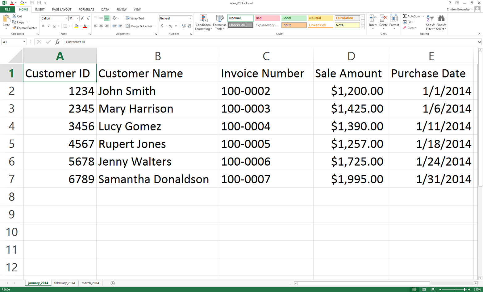
Now, to create a third workbook:
Change the names of the existing three worksheets to january_2015, february_2015, and march_2015.
In each of the three worksheets, change the year in the Purchase Date column to 2015.
There are six data rows in each worksheet, so you’ll be making a total of 18 changes (six rows * three worksheets). Other than the change in year, you don’t need to make any other changes.
Save this third workbook as sales_2015.xlsx.
Figure 3-11 shows what the january_2015 worksheet should look like after you’ve changed the dates.

In some cases, you may know the contents of the workbooks you’re dealing with; however, sometimes you didn’t create them so you don’t yet know their contents. Unlike CSV files, Excel workbooks can contain multiple worksheets, so if you’re unfamiliar with the workbooks, it’s important to get some descriptive information about them before you start processing them.
To count the number of workbooks in a folder, the number of worksheets in each workbook, and the number of rows and columns in each worksheet, type the following code into a text editor and save the file as 12excel_introspect_all_workbooks.py:
1#!/usr/bin/env python32importglob3importos4importsys5fromxlrdimportopen_workbook6input_directory=sys.argv[1]7workbook_counter=08forinput_fileinglob.glob(os.path.join(input_directory,'*.xls*')):9workbook=open_workbook(input_file)10('Workbook:%s'%os.path.basename(input_file))11('Number of worksheets:%d'%workbook.nsheets)12forworksheetinworkbook.sheets():13('Worksheet name:',worksheet.name,'\tRows:',\ 14worksheet.nrows,'\tColumns:',worksheet.ncols)15workbook_counter+=116('Number of Excel workbooks:%d'%(workbook_counter))
Lines 2 and 3 import Python’s built-in glob and os modules, respectively, so we can use their functions to identify and parse the pathnames of the files we want to process.
Line 8 uses Python’s built-in glob and os modules to create the list of input files that we want to process and applies a for loop over the list of input files. This line enables us to iterate over all of the workbooks we want to process.
Lines 10 to 14 print information about each workbook to the screen. Line 10 prints the name of the workbook. Line 11 prints the number of worksheets in the workbook. Lines 13 and 14 print the names of the worksheets in the workbook and the number of rows and columns in each worksheet.
To run the script, type the following on the command line and hit Enter:
python 12excel_introspect_all_workbooks.py "C:\Users\Clinton\Desktop"
You should then see the output shown in Figure 3-12 printed to your screen.
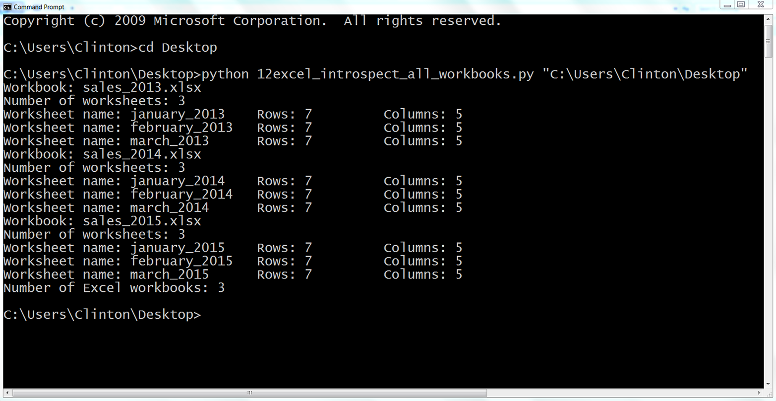
The output shows that the script processed three workbooks. It also shows the names of the three workbooks (e.g., sales_2013.xlsx), the names of the three worksheets in each workbook (e.g., january_2013), and the number of rows and columns in each worksheet (e.g., 7 rows and 5 columns).
Printing some descriptive information about files you plan to process is useful when you’re less familiar with the files. Understanding the number of files and the number of rows and columns in each file gives you some idea about the size of the processing job as well as the consistency of the file layouts.
To concatenate data from all of the worksheets in multiple workbooks vertically into one output file with base Python, type the following code into a text editor and save the file as 13excel_ concat_data_from_multiple_workbooks.py:
1#!/usr/bin/env python32importglob3importos4importsys5fromdatetimeimportdate6fromxlrdimportopen_workbook,xldate_as_tuple7fromxlwtimportWorkbook8input_folder=sys.argv[1]9output_file=sys.argv[2]10output_workbook=Workbook()11output_worksheet=output_workbook.add_sheet('all_data_all_workbooks')12data=[]13first_worksheet=True14forinput_fileinglob.glob(os.path.join(input_folder,'*.xls*')):15(os.path.basename(input_file))16withopen_workbook(input_file)asworkbook:17forworksheetinworkbook.sheets():18iffirst_worksheet:19header_row=worksheet.row_values(0)20data.append(header_row)21first_worksheet=False22forrow_indexinrange(1,worksheet.nrows):23row_list=[]24forcolumn_indexinrange(worksheet.ncols):25cell_value=worksheet.cell_value\ 26(row_index,column_index)27cell_type=worksheet.cell_type\ 28(row_index,column_index)29ifcell_type==3:30date_cell=xldate_as_tuple\ 31(cell_value,workbook.datemode)32date_cell=date(*date_cell[0:3])\ 33.strftime('%m/%d/%Y')34row_list.append(date_cell)35else:36row_list.append(cell_value)37data.append(row_list)38forlist_index,output_listinenumerate(data):39forelement_index,elementinenumerate(output_list):40output_worksheet.write(list_index,element_index,element)41output_workbook.save(output_file)
Line 13 creates a Boolean (i.e., True/False) variable named first_worksheet that we use to distinguish between the first worksheet and all of the subsequent worksheets we process. For the first worksheet we process, line 18 is True so we append the header row into data and then set first_worksheet equal to False.
For the remaining data rows in the first worksheet and all of the subsequent worksheets, we skip the header row and start processing the data rows. We know that we start at the second row because the range function in line 22 starts at one instead of zero.
To run the script, type the following on the command line and hit Enter:
python 13excel_ concat_data_from_multiple_workbooks.py "C:\Users\Clinton\Desktop"\ output_files\13output.xls
You can then open the output file, 13output.xls, to review the results.
Pandas provides the concat function for concatenating DataFrames. If you want to stack the DataFrames vertically on top of one another, then use axis=0. If you want to join them horizontally side by side, then use axis=1. Alternatively, if you need to join the DataFrames together based on a key column, the pandas merge function provides these SQL join–like operations (if this doesn’t make sense, don’t worry; we’ll talk more about database operations in Chapter 4).
To concatenate data from all of the worksheets in multiple workbooks vertically into one output file with pandas, type the following code into a text editor and save the file as pandas_concat_data_from_multiple_workbooks.py:
#!/usr/bin/env python3importpandasaspdimportglobimportosimportsysinput_path=sys.argv[1]output_file=sys.argv[2]all_workbooks=glob.glob(os.path.join(input_path,'*.xls*'))data_frames=[]forworkbookinall_workbooks:all_worksheets=pd.read_excel(workbook,sheetname=None,index_col=None)forworksheet_name,datainall_worksheets.items():data_frames.append(data)all_data_concatenated=pd.concat(data_frames,axis=0,ignore_index=True)writer=pd.ExcelWriter(output_file)all_data_concatenated.to_excel(writer,sheet_name='all_data_all_workbooks',\index=False)writer.save()
To run the script, type the following on the command line and hit Enter:
python pandas_concat_data_from_multiple_workbooks.py "C:\Users\Clinton\Desktop"\ output_files\pandas_output.xls
You can then open the output file, pandas_output.xls, to review the results.
To calculate worksheet- and workbook-level statistics for multiple workbooks with base Python, type the following code into a text editor and save the file as 14excel_sum_average_multiple_workbooks.py:
1#!/usr/bin/env python32importglob3importos4importsys5fromdatetimeimportdate6fromxlrdimportopen_workbook,xldate_as_tuple7fromxlwtimportWorkbook8input_folder=sys.argv[1]9output_file=sys.argv[2]10output_workbook=Workbook()11output_worksheet=output_workbook.add_sheet('sums_and_averages')12all_data=[]13sales_column_index=314header=['workbook','worksheet','worksheet_total','worksheet_average',\ 15'workbook_total','workbook_average']16all_data.append(header)17forinput_fileinglob.glob(os.path.join(input_folder,'*.xls*')):18withopen_workbook(input_file)asworkbook:19list_of_totals=[]20list_of_numbers=[]21workbook_output=[]22forworksheetinworkbook.sheets():23total_sales=024number_of_sales=025worksheet_list=[]26worksheet_list.append(os.path.basename(input_file))27worksheet_list.append(worksheet.name)28forrow_indexinrange(1,worksheet.nrows):29try:30total_sales+=float(str(worksheet.cell_value\ 31(row_index,sales_column_index))\ 32.strip('$').replace(',',''))33number_of_sales+=1.34except:35total_sales+=0.36number_of_sales+=0.37average_sales='%.2f'%(total_sales/number_of_sales)38worksheet_list.append(total_sales)39worksheet_list.append(float(average_sales))40list_of_totals.append(total_sales)41list_of_numbers.append(float(number_of_sales))42workbook_output.append(worksheet_list)43workbook_total=sum(list_of_totals)44workbook_average=sum(list_of_totals)/sum(list_of_numbers)45forlist_elementinworkbook_output:46list_element.append(workbook_total)47list_element.append(workbook_average)48all_data.extend(workbook_output)49 50forlist_index,output_listinenumerate(all_data):51forelement_index,elementinenumerate(output_list):52output_worksheet.write(list_index,element_index,element)53output_workbook.save(output_file)
Line 12 creates an empty list named all_data to hold all of the rows we want to write to the output file. Line 13 creates a variable named sales_column_index to hold the index value of the Sale Amount column.
Line 14 creates the list of column headings for the output file and line 16 appends this list of values into all_data.
In lines 19, 20, and 21 we create three lists. The list_of_totals will contain the total sale amounts for all of the worksheets in a workbook. Similarly, list_of_numbers will contain the number of sale amounts used to calculate the total sale amounts for all of the worksheets in a workbook. The third list, workbook_output, will contain all of the lists of output that we’ll write to the output file.
In line 25, we create a list, worksheet_list, to hold all of the information about the worksheet that we want to retain. In lines 26 and 27, we append the name of the workbook and the name of the worksheet into worksheet_list. Similarly, in lines 38 and 39, we append the total and average sale amounts into worksheet_list. In line 42, we append worksheet_list into workbook_output to store the information at the workbook level.
In lines 40 and 41 we append the total and number of sale amounts for the worksheet into list_of_totals and list_of_numbers, respectively, so we can store these values across all of the worksheets. In lines 43 and 44 we use the lists to calculate the total and average sale amount for the workbook.
In lines 45 to 47, we iterate through the lists in workbook_output (there are three lists for each workbook, as each workbook has three worksheets) and append the workbook-level total and average sale amounts into each of the lists.
Once we have all of the information we want to retain for the workbook (i.e., three lists, one for each worksheet), we extend the lists into all_data. We use extend instead of append so that each of the lists in workbook_output becomes a separate element in all_data. This way, after processing all three workbooks, all_data is a list of nine elements, where each element is a list. If instead we were to use append, there would only be three elements in all_data and each one would be a list of lists.
To run the script, type the following on the command line and hit Enter:
python 14excel_sum_average_multiple_workbooks.py "C:\Users\Clinton\Desktop"\ output_files\14output.xls
You can then open the output file, 14output.xls, to review the results.
Pandas makes it relatively straightforward to iterate through multiple workbooks and calculate statistics for the workbooks at both the worksheet and workbook levels. In this script, we calculate statistics for each of the worksheets in a workbook and concatenate the results into a DataFrame. Then we calculate workbook-level statistics, convert them into a DataFrame, merge the two DataFrames together with a left join on the name of the workbook, and add the resulting DataFrame to a list. Once all of the workbook-level DataFrames are in the list, we concatenate them together into a single DataFrame and write it to the output file.
To calculate worksheet and workbook-level statistics for multiple workbooks with pandas, type the following code into a text editor and save the file as pandas_sum_average_multiple_workbooks.py:
#!/usr/bin/env python3importpandasaspdimportglobimportosimportsysinput_path=sys.argv[1]output_file=sys.argv[2]all_workbooks=glob.glob(os.path.join(input_path,'*.xls*'))data_frames=[]forworkbookinall_workbooks:all_worksheets=pd.read_excel(workbook,sheetname=None,index_col=None)workbook_total_sales=[]workbook_number_of_sales=[]worksheet_data_frames=[]worksheets_data_frame=Noneworkbook_data_frame=Noneforworksheet_name,datainall_worksheets.items():total_sales=pd.DataFrame([float(str(value).strip('$').replace(\',',''))forvalueindata.loc[:,'Sale Amount']]).sum()number_of_sales=len(data.loc[:,'Sale Amount'])average_sales=pd.DataFrame(total_sales/number_of_sales)workbook_total_sales.append(total_sales)workbook_number_of_sales.append(number_of_sales)data={'workbook':os.path.basename(workbook),'worksheet':worksheet_name,'worksheet_total':total_sales,'worksheet_average':average_sales}worksheet_data_frames.append(pd.DataFrame(data,\columns=['workbook','worksheet',\'worksheet_total','worksheet_average']))worksheets_data_frame=pd.concat(\worksheet_data_frames,axis=0,ignore_index=True)workbook_total=pd.DataFrame(workbook_total_sales).sum()workbook_total_number_of_sales=pd.DataFrame(\workbook_number_of_sales).sum()workbook_average=pd.DataFrame(\workbook_total/workbook_total_number_of_sales)workbook_stats={'workbook':os.path.basename(workbook),'workbook_total':workbook_total,'workbook_average':workbook_average}workbook_stats=pd.DataFrame(workbook_stats,columns=\['workbook','workbook_total','workbook_average'])workbook_data_frame=pd.merge(worksheets_data_frame,workbook_stats,\on='workbook',how='left')data_frames.append(workbook_data_frame)all_data_concatenated=pd.concat(data_frames,axis=0,ignore_index=True)writer=pd.ExcelWriter(output_file)all_data_concatenated.to_excel(writer,sheet_name='sums_and_averages',\index=False)writer.save()
To run the script, type the following on the command line and hit Enter:
python pandas_sum_average_multiple_workbooks.py "C:\Users\Clinton\Desktop"\ output_files\pandas_output.xls
You can then open the output file, pandas_output.xls, to review the results.
We’ve covered a lot of ground in this chapter. We’ve discussed how to read and parse an Excel workbook, navigate rows in an Excel worksheet, navigate columns in an Excel worksheet, process multiple Excel worksheets, process multiple Excel workbooks, and calculate statistics for multiple Excel worksheets and workbooks. If you’ve followed along with the examples in this chapter, you have written 14 new Python scripts!
The best part about all of the work you have put into working through the examples in this chapter is that you are now well equipped to navigate and process Excel files, one of the most common file types in business. Moreover, because many business divisions store data in Excel workbooks, you now have a set of tools you can use to process the data in these workbooks regardless of the number of workbooks, the size of the workbooks, or the number of worksheets in each workbook. Now you can take advantage of your computer’s data processing capabilities to automate and scale your analysis of data in Excel workbooks.
The next data source we’ll tackle is databases. Because databases are a common data store, it’s important for you to know how to access their data. Once you know how to access the data, you can process it in the same row-by-row fashion that you’ve learned to use when dealing with CSV and Excel files. Having worked through the examples in these two chapters, you’re now well prepared to process data in databases.
Modify one of the scripts that filters rows based on conditions, sets, or regular expressions to print and write a different set of rows than the ones we filtered for in the examples.
Modify one of the scripts that filters columns based on index values or column headings to print and write a different set of columns that the ones we filtered for in the examples.
Create a new Python script that combines code from one of the scripts that filters rows or columns and code from the script that concatenates data from multiple workbooks to generate an output file that contains specific rows or columns of data from multiple workbooks.
Like spreadsheets, databases are ubiquitous in business. Companies use databases to store data on customers, inventory, and employees. Databases are vital to tracking operations, sales, financials, and more. What sets a database apart from a simple spreadsheet or a workbook of spreadsheets is that a database’s tables are linked such that a row in one spreadsheet can be linked to a row or column in another. To give a standard example, customer data—name, address, and so on—may be linked (using a customer ID number) to a row in an “orders” spreadsheet that contains items ordered. Those items are in turn linked up to data in your “suppliers” spreadsheet, enabling you to track and fulfill orders—and also to perform deeper analytics. While CSV and Excel files are common, important data sources that you can process automatically and at scale with Python, and building skills to handle these files has been important both from a learning perspective (to learn common programming operations) and from a practical perspective (a great deal of business data is stored in these types of files), databases truly leverage the power of computers to execute tasks hundreds, thousands, or even millions of times.
One thing you’ll need to learn how to interact with a database in Python is a database, and a table in the database filled with data. If you don’t already have access to such a database and table, this requirement could be a stumbling block. Fortunately, there are two resources at our disposal that will make it quick and easy to get up and running with the examples in this chapter.
First, Python has a built-in sqlite3 module that enables us to create an in-memory database. This means that we can create a database and table filled with data directly in our Python code without having to download and install database-specific software. We’ll use this feature in the first half of this chapter to get up and running quickly so that the focus can be on interacting with the database, table, and data instead of downloading and installing a database.
Second, you may already work with MySQL, PostgreSQL, or Oracle, some common database systems. The companies that make these database systems available have made it relatively easy to download and install their systems. While you may not work with a database system on a daily basis, they are very common in business, so it’s critically important for you to be familiar with some common database operations and how to carry out those operations in Python. Therefore, we’ll download and install a database system in the second half of this chapter so that you can use what you’ve learned in the first half of the chapter to become comfortable interacting with and manipulating data in an actual database system.
As already mentioned, we’ll get up and running quickly by using Python’s built-in sqlite3 module to create an in-memory database and table filled with data directly in our Python code. As in Chapter 2 and Chapter 3, the focus of this first example will be to demonstrate how to count the number of rows output by a SQL query. This capability is important in any situation where you are unsure how many rows your query will output, so that you know how many rows of data you’ll be processing before you begin computation. This example will also be helpful because we will use a lot of the syntax associated with interacting with databases in Python in order to create the database table, insert data into the table, and fetch and count the number of rows in the output. We’ll see much of this syntax repeated in examples throughout this chapter.
Let’s begin. To create a database table, insert data into the table, and fetch and count the number of rows in the output, type the following code into a text editor and save the file as 1db_count_rows.py:
1#!/usr/bin/env python32importsqlite33 4# Create an in-memory SQLite3 database5# Create a table called sales with four attributes6con=sqlite3.connect(':memory:')7query="""CREATE TABLE sales8(customer VARCHAR(20),9product VARCHAR(40),10amount FLOAT,11date DATE);"""12con.execute(query)13con.commit()14 15# Insert a few rows of data into the table16data=[('Richard Lucas','Notepad',2.50,'2014-01-02'),17('Jenny Kim','Binder',4.15,'2014-01-15'),18('Svetlana Crow','Printer',155.75,'2014-02-03'),19('Stephen Randolph','Computer',679.40,'2014-02-20')]20statement="INSERT INTO sales VALUES(?, ?, ?, ?)"21con.executemany(statement,data)22con.commit()23 24# Query the sales table25cursor=con.execute("SELECT * FROM sales")26rows=cursor.fetchall()27 28# Count the number of rows in the output29row_counter=030forrowinrows:31(row)32row_counter+=133('Number of rows:%d'%(row_counter))
Figure 4-1, Figure 4-2, and Figure 4-3 show what the script looks like in Anaconda Spyder, Notepad++ (Windows), and TextWrangler (macOS), respectively.
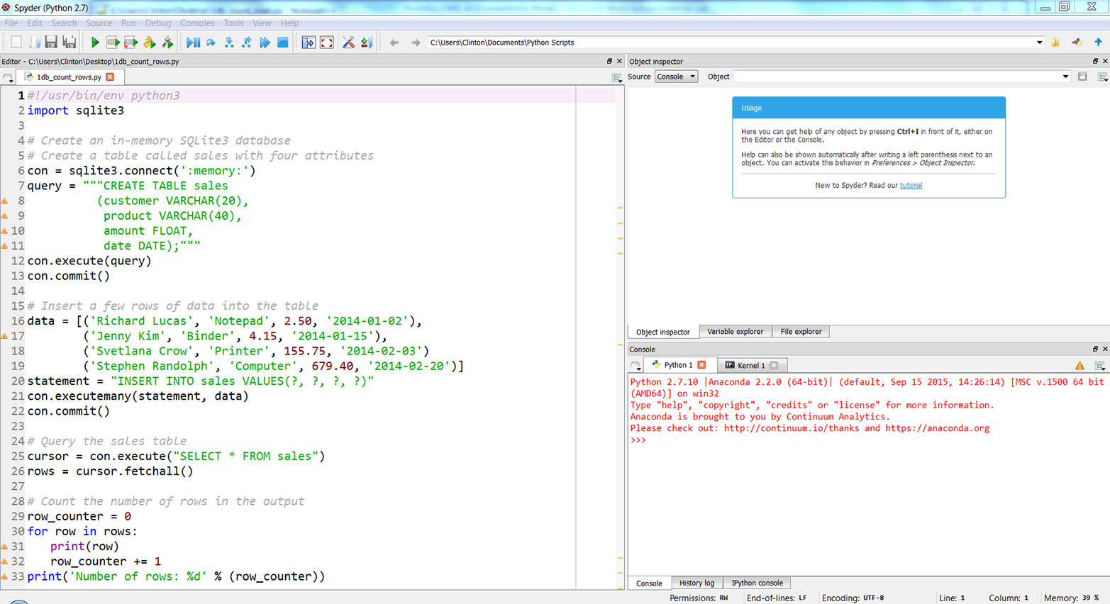
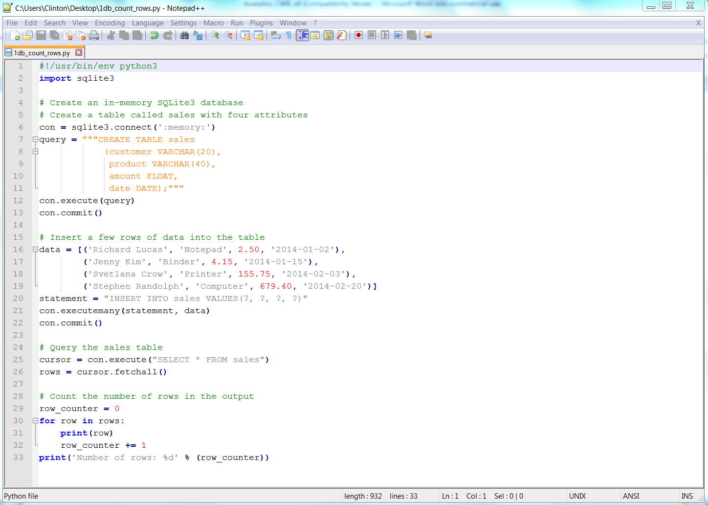
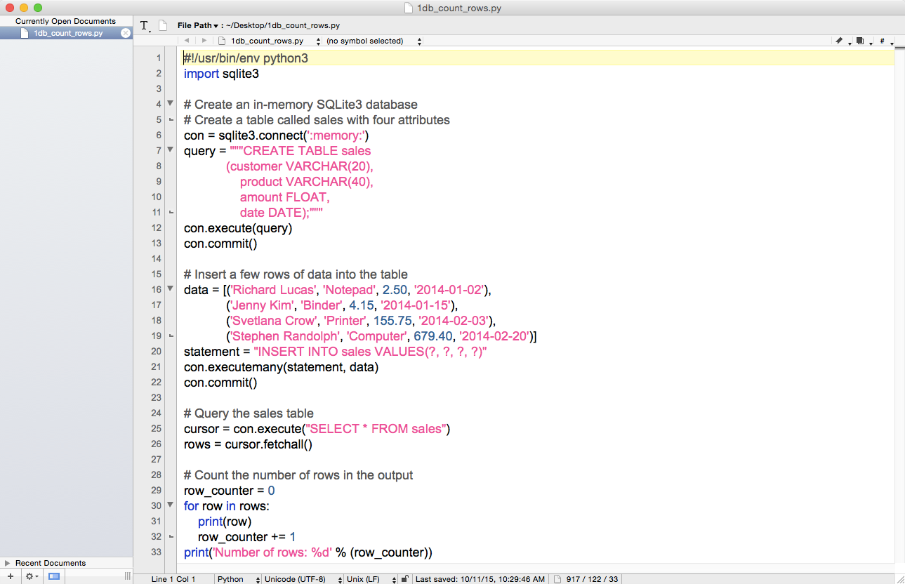
In these figures, you can already see some of the additional syntax we need to learn in order to interact with databases instead of CSV files or Excel workbooks.
Line 2 imports the sqlite3 module, which provides a lightweight disk-based database that doesn’t require a separate server process and allows accessing the database using a variant of the SQL query language. SQL commands appear in all caps in the code examples here. Because this chapter is about interacting with databases in Python, the chapter covers the majority of the common CRUD (i.e., Create, Read, Update, and Delete) database operations.1 The examples cover creating a database and table (Create), inserting records into the table (Create), updating records in the table (Update), and selecting specific rows from the table (Read). These SQL operations are common across relational databases.
In order to use this module, you must first create a connection object that represents the database. Line 6 creates a connection object called con to represent the database. In this example, I use the special name ':memory:' to create a database in RAM. If you want the database to persist, you can supply a different string. For example, if I were to use the string 'my_database.db' or 'C:\Users\Clinton\Desktop\my_database.db' instead of ':memory:', then the database object would persist in my current directory or on my Desktop.
Lines 7–11 use triple double-quotation marks to create a single string over multiple lines and assign the string to the variable query. The string is a SQL command that creates a table called sales in the database. The sales table has four attributes: customer, product, amount, and date. The customer attribute is a variable character length field with a maximum of 20 characters. The product attribute is also a variable character length field with a maximum of 40 characters. The amount attribute is a floating-point formatted field. The date attribute is a date-formatted field.
Line 12 uses the connection object’s execute() method to carry out the SQL command, contained in the variable query, to create the sales table in the in-memory database.
Line 13 uses the connection object’s commit() method to commit (i.e., save) the changes to the database. You always have to use the commit() method to save your changes when you make changes to the database; otherwise, your changes will not be saved in the database.
Line 16 creates a list of tuples and assigns the list to the variable data. Each element in the list is a tuple that contains four values: three strings and one floating-point number. These four values correspond by position to the four table attributes (i.e., the four columns in the table). Also, each tuple contains the data for one row in the table. Because the list contains four tuples, it contains the data for four rows in the table.
Line 20 is like line 7 in that it creates a string and assigns the string to the variable statement. Because this string fits on one line, it’s contained in one pair of double quotes instead of the pair of triple double quotes used in line 7 to manage the multi-line string. The string in this line is another SQL command, an INSERT statement we’ll use to insert the rows of data in data into the table sales. The first time you see this line you may be curious about the purpose of the question marks (?). The question marks serve as placeholders for values you want to use in your SQL commands. Then you provide a tuple of values in the connection object’s execute() or executemany() method, and the values in the tuple are substituted by position into your SQL command. This method of parameter substitution makes your code less vulnerable to a SQL injection attack,2 which actually sounds as harmful as it can be, than assembling your SQL command with string operations.
Line 21 uses the connection object’s executemany() method to execute (i.e., run) the SQL command contained in statement for every tuple of data contained in data. Because there are four tuples of data in data, this executemany() method runs the INSERT statement four times, effectively inserting four rows of data into the tables sales.
Remember that when discussing line 13 we noted that you always have to use the commit() method when you make changes to the database; otherwise, your changes will not be saved in the database. Inserting four rows of data into the table sales definitely constitutes a change to the database, so in line 22 we once again use the connection object’s commit() method to save the changes to the database.
Now that we have the table sales in our in-memory database and it has four rows of data in it, let’s learn how to extract data from a database table. Line 25 uses the connection object’s execute() method to run a one-line SQL command and assigns the result of the command to a cursor object called cursor. Cursor objects have several methods (e.g., execute, executemany, fetchone, fetchmany, and fetchall). However, because you’re often interested in viewing or manipulating the entire result set of the SQL command you ran in the execute() method, you’ll commonly want to use the fetchall() method to fetch (i.e., return) all of the rows in the result set.
Line 26 implements this code. It uses the cursor object’s fetchall() method to return all of the rows in the result set of the SQL command executed in line 25 and assigns the rows to the list variable rows. That is, the variable rows is a list that contains all of the rows of data resulting from the SQL command in line 25. Each row of data is a tuple of values, so rows is a list of tuples. In this case, because we know the table sales contains four rows of data and the SQL command selects all rows of data from the sales table, we know that rows is a list of four tuples.
Finally, in lines 29–33, we return to the now basic operations of creating a row_counter variable to count the number of rows in rows, creating a for loop to iterate over each row in rows, incrementing the value in row_counter by one for each row in rows, and finally, after the for loop has completed iterating over all of the rows in rows, printing the string Number of rows: and the value in row_counter to the Command Prompt (or Terminal) window. As I’ve said, we expect that there are four rows of data in rows.
To see this Python script in action, type one of the following commands on the command line, depending on your operating system, and then hit Enter:
python 1db_count_rows.py
chmod +x 1db_count_rows.py ./1db_count_rows.py
You should see the output shown in Figure 4-4 (on Windows) or Figure 4-5 (on macOS) printed to the screen.
This output shows that there are four records in the sales table. More generally, the output also shows that we created an in-memory database, created the table sales, populated the table with four records, fetched all of the rows from the table, and counted the number of rows in the output.
Now that we understand the basic operations for creating an in-memory database, creating a table, loading data into the table, and fetching data from the table, let’s broaden our capabilities by learning how to insert data into a table and update records in a table at scale with CSV input files.
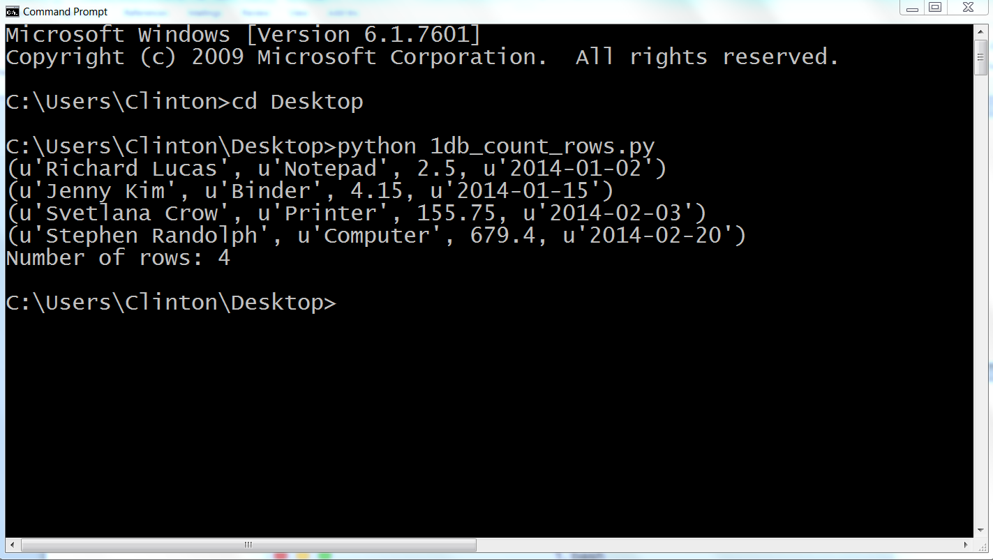
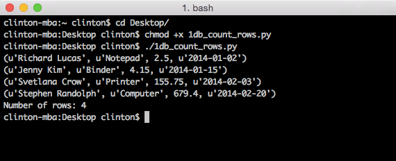
The previous example explained the basic operations for loading data into a table, but it included a severe limitation in that we handwrote the values to be loaded into the table. What happens if we need to load 10,000 records, each with 20 to 30 column attributes, into a table? Needless to say, manual data entry doesn’t scale.
In many cases, the data that needs to be loaded into a database table is the result of a database query or already resides in one or more Excel or CSV files. Because it is relatively easy to export the result of a database query to a CSV file for all major databases, and we’ve already learned how to process Excel and CSV files, let’s learn how to go the other way and load data into a database table at scale with a CSV input file.
Let’s create a new Python script. The script will create a database table, insert data from a CSV file into the table, and then show us the data that is now in the table. This third step, printing the data to the Command Prompt/Terminal window, isn’t necessary (and I wouldn’t recommend printing records to the window if you’re loading thousands of records), but I’ve included this step to illustrate one way to print all of the columns for each record without needing to specify individual column indexes (i.e., this syntax generalizes to any number of columns). To begin, type the following code into a text editor and save the file as 2db_insert_rows.py:
1#!/usr/bin/env python32importcsv3importsqlite34importsys5# Path to and name of a CSV input file6input_file=sys.argv[1]7# Create an in-memory SQLite3 database8# Create a table called Suppliers with five attributes9con=sqlite3.connect('Suppliers.db')10c=con.cursor()11create_table="""CREATE TABLE IF NOT EXISTS Suppliers12(Supplier_Name VARCHAR(20),13Invoice_Number VARCHAR(20),14Part_Number VARCHAR(20),15Cost FLOAT,16Purchase_Date DATE);"""17c.execute(create_table)18con.commit()19# Read the CSV file20# Insert the data into the Suppliers table21file_reader=csv.reader(open(input_file,'r'),delimiter=',')22header=next(file_reader,None)23forrowinfile_reader:24data=[]25forcolumn_indexinrange(len(header)):26data.append(row[column_index])27(data)28c.execute("INSERT INTO Suppliers VALUES (?, ?, ?, ?, ?);",data)29con.commit()30('')31# Query the Suppliers table32output=c.execute("SELECT * FROM Suppliers")33rows=output.fetchall()34forrowinrows:35output=[]36forcolumn_indexinrange(len(row)):37output.append(str(row[column_index]))38(output)
This script, like the scripts we wrote in Chapter 2, relies on the csv and sys modules. Line 2 imports the csv module so we can use its methods to read and parse the CSV input file. Line 4 imports the sys module so we can supply the path to and name of a file on the command line for use in the script. Line 3 imports the sqlite3 module so we can use its methods to create a simple, local database and table and execute SQL queries.
Line 6 uses the sys module to read the path to and name of a file on the command line and assigns that value to the variable input_file.
Line 9 creates a connection to a simple, local database called Suppliers.db. I’ve supplied a name for the database instead of using the special keyword ':memory:' to demonstrate how to create a database that will persist and not be deleted when you restart your computer. Because you will be saving this script on your Desktop, Suppliers.db will also be saved on your Desktop. If you want to save the database in a different location you can use a path of your choosing, like 'C:\Users\<Your Name>\Documents\Suppliers.db', instead of 'Suppliers.db'.
Lines 10–18 create a cursor and a multi-line SQL statement to create a table called Suppliers that has five column attributes, execute the SQL statement, and commit the changes to the database.
Lines 21–29 deal with reading the data to be loaded into the database table from a CSV input file and executing a SQL statement for each row of data in the input file to insert it into the database table. Line 21 uses the csv module to create the file_reader object. Line 22 uses the next() method to read the first row from the input file, the header row, and assign it to the variable header. Line 23 creates a for loop for looping over all of the data rows in the input file. Line 24 creates an empty list variable called data. For each row of input, we’ll populate data with the values in the row needed for the INSERT statement in line 28. Line 25 creates a for loop for looping over all of the columns in each row. Line 26 uses the list’s append() method to populate data with all of the values in the input file for that row. Line 27 prints the row of data that’s been appended into data to the Command Prompt/Terminal window. Notice the indentation. This line is indented beneath the outer for loop, rather than the inner for loop, so that it occurs for every row rather than for every row and column in the input file. This line is helpful for debugging, but once you’re confident the code is working correctly you can delete it or comment it out so you don’t have a lot of output printed to the window.
Line 28 is the line that actually loads each row of data into the database table. This line uses the cursor object’s execute() method to execute an INSERT statement to insert a row of values into the table Suppliers. The question marks ? are placeholders for each of the values to be inserted. The number of question marks should correspond to the number of columns in the input file, which should correspond to the number of columns in the table. Moreover, the order of the columns in the input file should correspond to the order of the columns in the table. The values substituted into the question mark positions come from the list of values in data, which appears after the comma in the execute() statement. Because data is populated with values for each row of data in the input file and the INSERT statement is executed for each row of data in the input file, these lines of code effectively read the rows of data from the input file and load the rows of data into the database table. Finally, line 29 is another commit statement to commit the changes to the database.
Lines 32 to 38 demonstrate how to select all of the data from the table Suppliers and print the output to the Command Prompt/Terminal window. Lines 32 and 33 execute a SQL statement to select all of the data from the Suppliers table and fetch all of the rows in “output” to the variable “rows”. Line 34 creates a for loop for looping over each row in “rows”. Line 36 creates a for loop for looping over all of the columns in each row. Line 37 appends each of the column values into a list named “output”. Finally, the print statement in line 38 ensures that each row of output is printed on a new line (notice the indentation, it’s in the row, not column, for loop).
Now all we need is a CSV input file that contains all of the data we want to load into our database table. For this example, let’s use the supplier_data.csv file we used in Chapter 2. In case you skipped Chapter 2 or don’t have the file, the data in the supplier_data.csv file looks as shown in Figure 4-6.
Now that we have our Python script and CSV input file, let’s use our script to load the data in our CSV input file into our Suppliers database table. To do so, type the following on the command line and then hit Enter:
python 2db_insert_rows.py supplier_data.csv
Figure 4-7 shows what the output looks like when printed to a Command Prompt window. The first block of output is the data rows as they’re parsed from the CSV file, and the second block of output is the same rows as they’re extracted from the sqlite table.
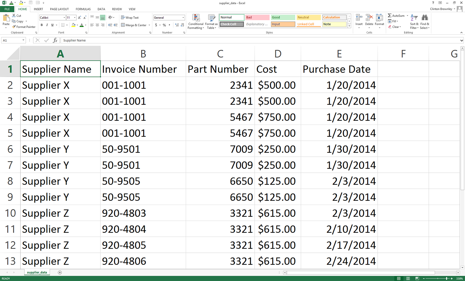
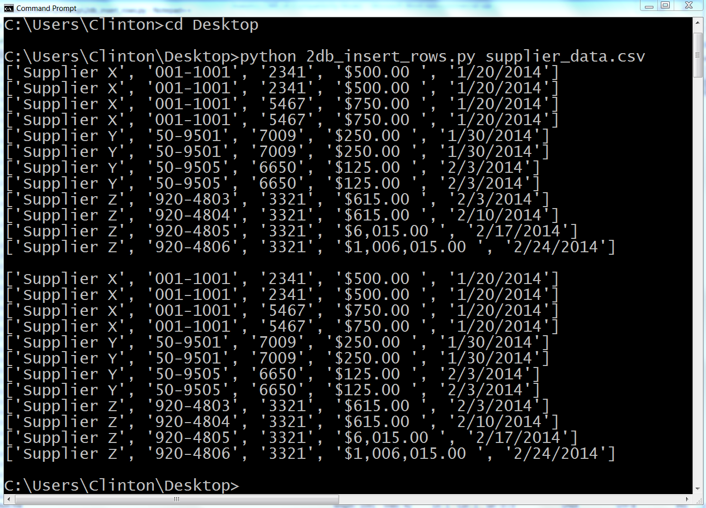
This output shows the 12 lists of values created for the 12 rows of data, excluding the header row, in the CSV input file. Beneath the 12 lists created from the input data there is a space, and then there are the 12 lists for the rows fetched from the database table.
This example demonstrated how to load data into a database table at scale by reading all of the data to be loaded into the table from a CSV input file and inserting the data in the file into the table. This example covers situations in which you want to add new rows to a table, but what if instead you want to update existing rows in a table? The next example covers this situation.
The previous example explained how to add rows to a database table using a CSV input file—an approach that, because you can use loops and glob, you can scale to any number of files. But sometimes, instead of loading new data into a table you need to update existing rows in a table.
Fortunately, we can reuse the technique of reading data from a CSV input file to update existing rows in a table. In fact, the technique of assembling a row of values for the SQL statement and then executing the SQL statement for every row of data in the CSV input file remains the same as in the previous example. The SQL statement is what changes. It changes from an INSERT statement to an UPDATE statement.
We’re already familiar with how to use a CSV input file to load data into a database table, so let’s learn how to use a CSV input file to update existing records in a database table. To do so, type the following code into a text editor and save the file as 3db_update_rows.py:
1#!/usr/bin/env python32importcsv3importsqlite34importsys5# Path to and name of a CSV input file6input_file=sys.argv[1]7# Create an in-memory SQLite3 database8# Create a table called sales with four attributes9con=sqlite3.connect(':memory:')10query="""CREATE TABLE IF NOT EXISTS sales11(customer VARCHAR(20),12product VARCHAR(40),13amount FLOAT,14date DATE);"""15con.execute(query)16con.commit()17# Insert a few rows of data into the table18data=[('Richard Lucas','Notepad',2.50,'2014-01-02'),19('Jenny Kim','Binder',4.15,'2014-01-15'),20('Svetlana Crow','Printer',155.75,'2014-02-03'),21('Stephen Randolph','Computer',679.40,'2014-02-20')]22fortupleindata:23(tuple)24statement="INSERT INTO sales VALUES(?, ?, ?, ?)"25con.executemany(statement,data)26con.commit()27# Read the CSV file and update the specific rows28file_reader=csv.reader(open(input_file,'r'),delimiter=',')29header=next(file_reader,None)30forrowinfile_reader:31data=[]32forcolumn_indexinrange(len(header)):33data.append(row[column_index])34(data)35con.execute("UPDATE sales SET amount=?, date=? WHERE customer=?;",data)36con.commit()37# Query the sales table38cursor=con.execute("SELECT * FROM sales")39rows=cursor.fetchall()40forrowinrows:41output=[]42forcolumn_indexinrange(len(row)):43output.append(str(row[column_index]))44(output)
All of the code should look familiar. Lines 2–4 import three of Python’s built-in modules so we can use their methods to read command-line input, read a CSV input file, and interact with an in-memory database and table. Line 6 assigns the CSV input file to the variable input_file.
Lines 9–16 create an in-memory database and a table called sales that has four column attributes.
Lines 18–24 create a set of four records for the sales table and insert the four records into the table. Take a moment to look at the records for Richard Lucas and Jenny Kim. These are the two records that we’ll update later in this script. At this point, with its four records, the sales table is similar to (albeit probably much smaller than) any table you will face when you want to update existing records in a database table.
Lines 28–36 are nearly identical to the code in the previous example. The only significant difference is in line 35, where an UPDATE statement has replaced the previous INSERT statement. The UPDATE statement is where you have to specify which records and column attributes you want to update. In this case, we want to update the amount and date values for a specific set of customers. Like in the previous example, there should be as many placeholder question marks as there are values in the query, and the order of the data in the CSV input file should be the same as the order of the attributes in the query. In this case, from left to right the attributes in the query are amount, date, and customer; therefore, the columns from left to right in the CSV input file should be amount, date, and customer.
Finally, the code in lines 39–44 is basically identical to the same section of code in the previous example. These lines of code fetch all of the rows in the sales table and print each row to the Command Prompt/Terminal window with a single space between column values.
Now all we need is a CSV input file that contains all of the data we need to update some of the records in our database table. To create the file:
Open a spreadsheet.
Add the data shown in Figure 4-8.
Save the file as data_for_updating.csv.
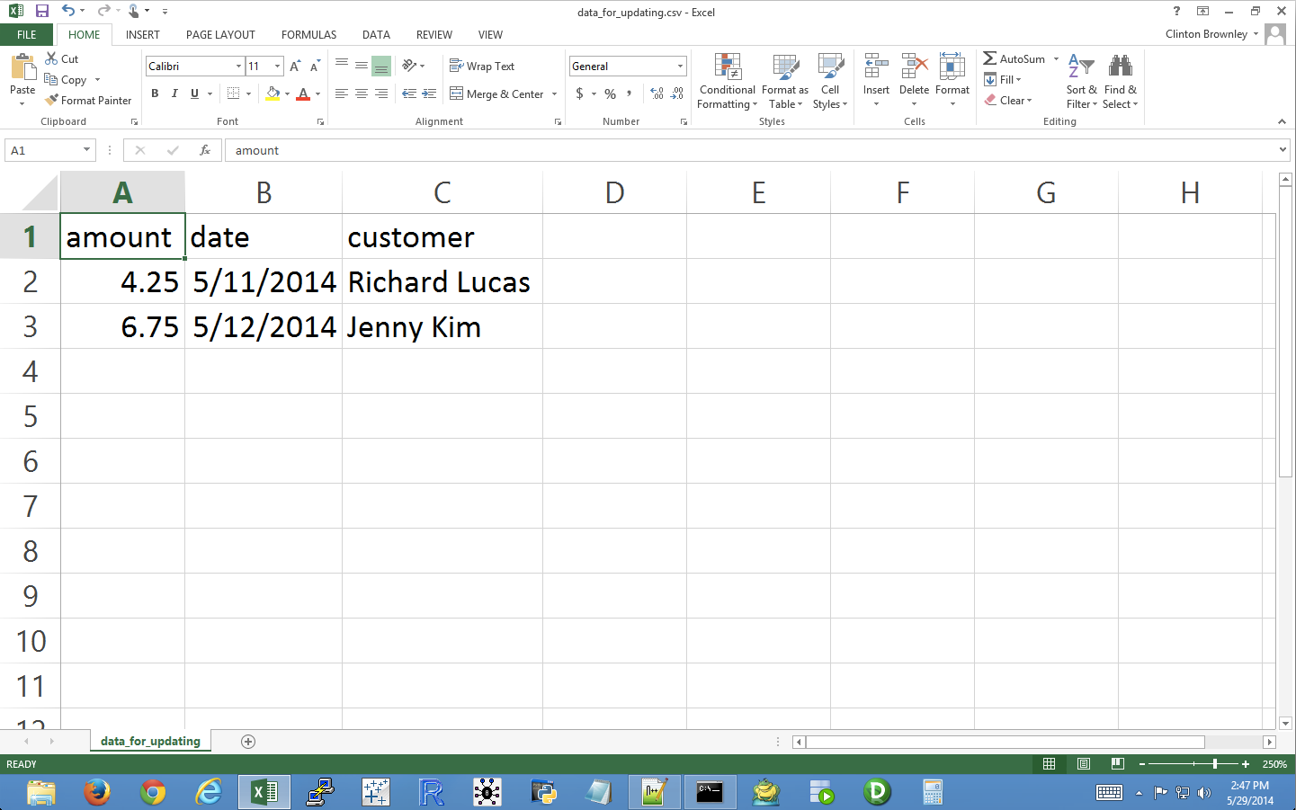
Now that we have our Python script and CSV input file, let’s use our script and input file to update specific records in our sales database table. To do so, type the following on the command line and then hit Enter:
python 3db_update_rows.py data_for_updating.csv
Figure 4-9 shows what the output looks like when printed to a Command Prompt window. The first four rows of output (tuples) are the initial data rows, the next two rows (lists) are the data from the CSV file, and the last four rows (lists) are the data from the database table after the rows have been updated.
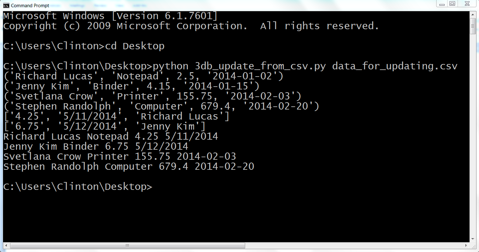
This output shows the four initial rows of data in the database, followed by the two lists of values to be updated in the database. The two lists of values to be updated show that the new amount value for Richard Lucas will be 4.25 and the date value will be 5/11/2014. Similarly, the new amount value for Jenny Kim will be 6.75 and the date value will be 5/12/2014.
Beneath the two update lists, the output also shows the four rows fetched from the database table after the updates were executed. Each row is printed on a separate line and the values in each row are separated by single spaces. Recall that the original amount and date values for Richard Lucas were 2.5 and 2014-01-02, respectively. Similarly, the original amount and date values for Jenny Kim were 4.15 and 2014-01-15, respectively. As you can see in the output shown in Figure 4-9, these two values have been updated for Richard Lucas and Jenny Kim to reflect the new values supplied in the CSV input file.
This example demonstrated how to update records in an existing database table at scale by using a CSV input file to supply the data needed to update specific records. Up to this point in the chapter, the examples have relied on Python’s built-in sqlite3 module. We’ve used this module to be able to quickly write scripts that do not rely on a separate, downloaded database like MySQL, PostgreSQL, or Oracle. In the next section, we’ll build on these examples by downloading a database program, MySQL, and learning how to load data into a database table and update records in a database program, as well as write query output to a CSV file. Let’s get started.
To complete the examples in this section, you need to have the MySQLdb package, a.k.a. MySQL-python (Python v2) or mysqlclient (Python v3).3 This package enables Python to interact with databases and their respective tables, so we will use it to interact with the MySQL database table we create in this section. If you installed Anaconda’s Python, then you already have the package because it’s bundled into the installation. If you installed Python from the Python.org website, then you need to follow the instructions in Appendix A to download and install the package.
As before, in order to work with a database table, we first need to create one:
Download the MySQL database program as described in Appendix A.
After you download the MySQL database program, you’ll have access to the MySQL command-line client.
Open the MySQL command-line client by entering mysql at the command line.
Now you are interacting with your MySQL database program with a command-line interface. To begin, let’s view the existing databases in your MySQL database program.
To do so, type the following and then hit Enter. Figure 4-10 shows the results on a Windows computer.
SHOW DATABASES;
Notice that the command ended with a semicolon. That’s how MySQL knows that you’re done with the command—if you hit Enter without the semicolon, then MySQL will expect another line of command (you’ll see multi-line commands shortly). If you forget that semicolon, don’t worry; you can type just the semicolon and Enter on the next line and MySQL will execute your command.
The output from this command shows that there are already four databases in the MySQL database program. These databases enable the MySQL database program to run and also contain information about the access rights of the users of the program. To create a database table, we first have to create a database of our own.
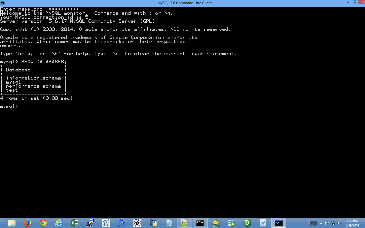
To create a database, type the following and then hit Enter:
CREATE DATABASE my_suppliers;
After you hit Enter, you can run the SHOW DATABASES; command again to see that you’ve created a new database. To create a database table in the my_suppliers database, we first have to choose to work in the my_suppliers database.
To work in the my_suppliers database, type the following and then hit Enter (see Figure 4-11):
USE my_suppliers;
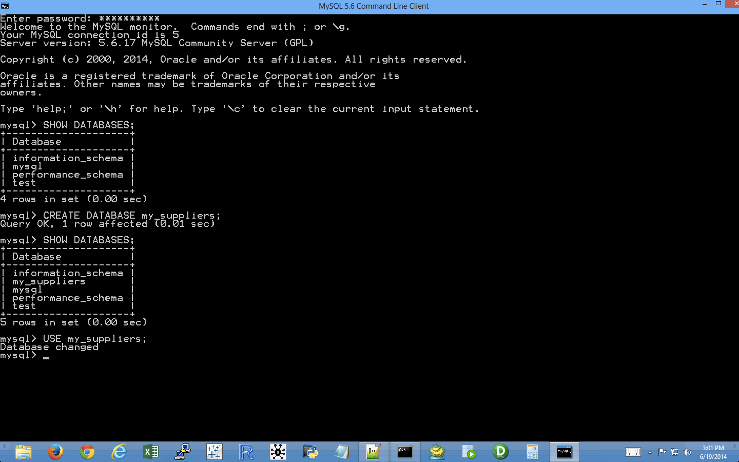
After you hit Enter, you’ll be in the my_suppliers database. Now we can create a database table to store data on our suppliers.
To create a database table called Suppliers, type the following and then hit Enter:
CREATE TABLE IF NOT EXISTS Suppliers (Supplier_Name VARCHAR(20), Invoice_Number VARCHAR(20), Part_Number VARCHAR(20), Cost FLOAT, Purchase_Date DATE);
This command creates a database table called Suppliers if a table called Suppliers does not already exist in the database. The table has five columns (a.k.a. fields or attributes): Supplier_Name, Invoice_Number, Part_Number, Cost, and Purchase_Date.
The first three columns are variable character VARCHAR fields. The 20 means we’ve allocated 20 characters for data entered into the field. If the data entered into the field is longer than 20 characters, then the data is truncated. If the data is shorter than 20 characters, then the field allocates the smaller amount of space for the data. Using VARCHAR for fields that contain variable-length strings is helpful because the table will not waste space storing more characters than is necessary. However, you do want to make sure that the number in parentheses is large enough to allocate enough characters so that the longest string in the field isn’t truncated. Some alternatives to VARCHAR are CHAR, ENUM, and BLOB. You might consider these alternatives when you want to specify a specific number of characters for the field and have values in the field right-padded to the specified length, specify a list of permissible values for the field (e.g., small, medium, large), or permit a variable and potentially large amount of text to go into the field, respectively.
The fourth column is a floating-point number FLOAT field. A floating-point number field holds floating-point, approximate values. Because in this case the fourth column contains monetary values, an alternative to FLOAT is NUMERIC, a fixed-point exact value type of field. For example, instead of FLOAT, you could use NUMERIC(11,2). The 11 is the precision of the numeric value, or the total number of digits stored, including the digits after the decimal point, for the value. The 2 is the scale, or the total number of digits after the decimal point. We use FLOAT instead of NUMERIC in this case for maximum code portability.
The final column is a date DATE field. A DATE field holds a date, with no time part, in 'YYYY-MM-DD' format. So a date like 6/19/2014 is stored in MySQL as '2014-06-19'. Invalid dates are converted to '0000-00-00'.
To ensure that the database table was created correctly, type the following and then hit Enter:
DESCRIBE Suppliers;
After you hit Enter, you should see a table that lists the names of the columns you created, the data type (e.g., VARCHAR or FLOAT) for each of the columns, and whether values in the columns can be NULL.
Now that we’ve created a database, my_suppliers, and a table in the database, Suppliers, let’s create a new user and give the user privileges to interact with the database and the table.
To create a new user, type the following and then hit Enter (make sure to replace username with the username you’d like to use; you should also change the password, secret_password, to something more secure):
CREATE USER 'username'@'localhost' IDENTIFIED BY 'secret_password';
Now that we’ve created a new user, let’s grant the user all privileges on our database, my_suppliers. By granting the user all privileges on the database, we enable the user to perform many different operations on the tables in the database. These privileges are useful because the scripts in this section involve loading data into the table, modifying specific records in the table, and querying the table.
To grant all privileges to the new user, type the following two commands and hit Enter after each one (again, make sure to replace username with the username you created in the previous step):
GRANT ALL PRIVILEGES ON my_suppliers.* TO 'username'@'localhost';
FLUSH PRIVILEGES;
You can now interact with the Suppliers table in the my_suppliers database from localhost (i.e., your local computer). See Figure 4-12.
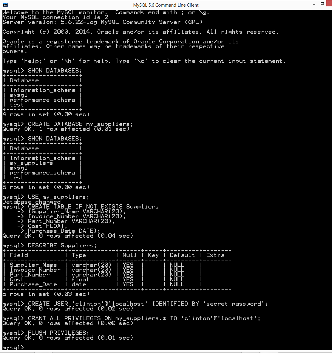
Now that we have a database and table in which to store data, let’s learn how to load data into the table with Python.
Now we’re ready to load records from a CSV file into a database table. You can already output records from Python scripts or Excel files into a CSV file, so this will enable you to create a very versatile data pipeline.
Let’s create a new Python script. The script will insert data from a CSV file into our database table and then show us the data that is now in the table. This second step, printing the data to the Command Prompt/Terminal window, isn’t necessary (and I wouldn’t recommend printing records to the window if you’re loading thousands of records!), but I’ve included this step to illustrate one way to print all of the columns for each record without needing to specify individual column indexes (i.e., this syntax generalizes to any number of columns).
To begin, type the following code into a text editor and save the file as 4db_mysql_load_from_csv.py:
1#!/usr/bin/env python32importcsv3importMySQLdb4importsys5fromdatetimeimportdatetime,date6 7# Path to and name of a CSV input file8input_file=sys.argv[1]9# Connect to a MySQL database10con=MySQLdb.connect(host='localhost',port=3306,db='my_suppliers',\ 11user='root',passwd='my_password')12c=con.cursor()13# Insert the data into the Suppliers table14file_reader=csv.reader(open(input_file,'r',newline=''))15header=next(file_reader)16forrowinfile_reader:17data=[]18forcolumn_indexinrange(len(header)):19ifcolumn_index<4:20data.append(str(row[column_index]).lstrip('$')\ 21.replace(',','').strip())22else:23a_date=datetime.date(datetime.strptime(\ 24str(row[column_index]),'%m/%d/%Y'))25# %Y: year is 2015; %y: year is 1526a_date=a_date.strftime('%Y-%m-%d')27data.append(a_date)28data29c.execute("""INSERT INTO Suppliers VALUES (%s,%s,%s,%s,%s);""",data)30con.commit()31("")32# Query the Suppliers table33c.execute("SELECT * FROM Suppliers")34rows=c.fetchall()35forrowinrows:36row_list_output=[]37forcolumn_indexinrange(len(row)):38row_list_output.append(str(row[column_index]))39(row_list_output)
This script, like the scripts we wrote in Chapter 2, relies on the csv, datetime, string, and sys modules. Line 2 imports the csv module so we can use its methods to read and parse the CSV input file. Line 4 imports the sys module so we can supply the path to and name of a file on the command line for use in the script. Line 5 imports the datetime and date methods from the datetime module so we can manipulate and format the dates in the last column of the input file. We need to strip the dollar sign off of the value and remove any embedded commas so it can enter the column in the database table that accepts floating-point numbers. Line 3 imports the add-in MySQLdb module that we downloaded and installed so that we can use its methods to connect to MySQL databases and tables.
Line 8 uses the sys module to read the path to and name of a file on the command line and assigns that value to the variable input_file.
Line 10 uses the MySQLdb module’s connect() method to connect to my_suppliers, the MySQL database we created in the previous section. Unlike when working with CSV or Excel files, which you can read, modify, or delete in place, MySQL sets up a database as though it were a separate computer (a server), which you can connect to, send data to, and request data from. The connection specifies several common arguments, including host, port, db, user, and passwd.
The host is the hostname of the machine that holds the database. In this case, the MySQL server is stored on your machine, so the host is localhost. When you’re connecting to other data sources, the server will be on a different machine, so you will need to change localhost to the hostname of the machine that holds the server.
The port is the port number for the TCP/IP connection to the MySQL server. The port number we’ll use is the default port number, 3306. As with the host argument, if you are not working on your local machine and your MySQL server administrator set up the server with a different port number, then you’ll have to use that port to connect to the MySQL server. However, in this case we installed MySQL server with the default values, so localhost is a valid hostname and 3306 is a valid port number.
The db is the name of the database you want to connect to. In this case, we want to connect to the my_suppliers database because it holds the database table into which we want to load data. If in the future, you create another database on your local computer, such as contacts, then you’ll have to change my_suppliers to contacts as the db argument to connect to that database.
The user is the username of the person making the database connection. In this case, we are connecting as the “root” user, with the password we created when we installed the MySQL server. When you install MySQL (which you may have done by following the instructions in Appendix A), the MySQL installation process asks you to provide a password for the root user. The password I created for the root user, which I’m supplying to the passwd argument in the code shown here is 'my_password'. Of course, if you supplied a different password for the root user when you installed MySQL, then you should substitute your password for 'my_password' in the code in this script.
During the database, table, and new user setup steps, I created a new user, clinton, with the password secret_password. Therefore, I could also use the following connection details in the script: user='clinton' and passwd='secret_password'. If you want to leave user='root' in the code, then you should substitute the password you actually supplied when you set up the MySQL server for 'my_password'. Alternatively, you can use the username and password you supplied when you created a new user with the CREATE USER command. With these five inputs, you create a local connection to the my_suppliers database.
Line 12 creates a cursor that we can use to execute SQL statements against the Suppliers table in the my_suppliers database and to commit the changes to the database.
Lines 14–29 deal with reading the data to be loaded into the database table from a CSV input file and executing a SQL statement for each row of data in the input file to insert it into the database table. Line 14 uses the csv module to create the file_reader object. Line 15 uses the next() method to read the first row from the input file—the header row—and assigns it to the variable header. Line 16 creates a for loop for looping over all of the data rows in the input file. Line 17 creates an empty list variable called data. For each row of input, we’ll populate data with the values in the row needed for the INSERT statement in line 28. Line 18 creates a for loop for looping over all of the columns in each row. Line 19 creates an if-else statement to test whether the column index is less than four. Because the input file has five columns and the dates are in the last column, the index value for the column of dates is four. Therefore, this line evaluates whether we’re dealing with the columns that precede the last column of dates. For all of the preceding columns, with index values 0, 1, 2, and 3, line 20 converts the value to a string, strips off a dollar sign character from the lefthand side of the string if it exists, and then appends the value into the list variable, data. For the last column of dates, line 23 converts the value to a string, creates a datetime object from the string based on the input format of the string, converts the datetime object into a date object (retaining only the year, month, and day elements), and assigns the value to the variable a_date. Next, line 26 converts the date object into a string with the new format we need to load the date strings into a MySQL database (i.e., YYYY-MM-DD) and reassigns the newly formatted string to the variable a_date. Finally, line 27 appends the string into data.
Line 28 prints the row of data that’s been appended into data to the Command Prompt/Terminal window. Notice the indentation. This line is indented beneath the outer for loop, rather than the inner for loop, so that it occurs for every row rather than for every row and column in the input file. This line is helpful for debugging, but once you’re confident the code is working correctly you can delete it or comment it out so you don’t have a lot of output printed to your Command Prompt window.
Line 29 is the line that actually loads each row of data into the database table. This line uses the cursor object’s execute() method to execute an INSERT statement to insert a row of values into the table Suppliers. Each %s is placeholder for a value to be inserted. The number of placeholders should correspond to the number of columns in the input file, which should correspond to the number of columns in the table. Moreover, the order of the columns in the input file should correspond to the order of the columns in the table. The values substituted into the %s positions come from the list of values in data, which appears after the comma in the execute() statement. Because data is populated with values for each row of data in the input file and the INSERT statement is executed for each row of data in the input file, this line of code effectively reads the rows of data from the input file and loads the rows of data into the database table. Once again, notice the indentation. The line is indented beneath the outer for loop, so it occurs for every row of data in the input file. Finally, line 30 is another commit statement to commit the changes to the database.
Lines 33 to 39 demonstrate how to select all of the data from the table Suppliers and print the output to the Command Prompt/Terminal window. Lines 33 and 34 execute a SQL statement to select all of the data from the Suppliers table and fetch all of the rows of output into the variable rows. Line 35 creates a for loop for looping over each row in rows. Line 36 creates an empty list variable, row_list_output, that will contain all of the values in each row of output from the SQL query. Line 37 creates a for loop for looping over all of the columns in each row. Line 38 converts each value to a string and then appends the value into row_list_output. Finally, once all of the values from a row are in row_list_output, line 39 prints the row to the screen.
Now that we have our Python script, let’s use our script to load the data in supplier_data.csv into our Suppliers database table. To do so, type the following on the command line and then hit Enter:
python 4db_mysql_load_from_csv.py supplier_data.csv
On Windows, you should see the output shown in Figure 4-13 printed to the Command Prompt window. The first block of output is the data as it’s parsed from the CSV file, and the second block of output is the same data as it’s queried from the database table.
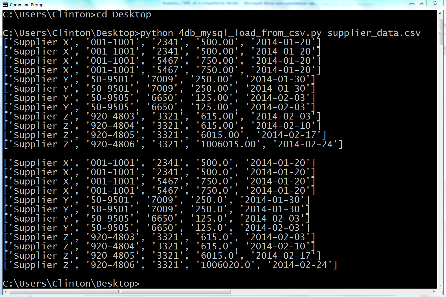
This output shows the 12 lists of values created for the 12 rows of data, excluding the header row, in the CSV input file. You can recognize the 12 lists because each list is enclosed in square brackets ([]) and the values in each list are separated by commas.
Beneath the 12 lists of input data read from the CSV file, there is a space, and then there are the 12 rows of output that were fetched from the database table with the query, SELECT * FROM Suppliers. Again, each row is printed on a separate line and the values in each row are separated by commas. This output confirms that the data was successfully loaded into and then read from the Suppliers table.
To confirm the results in a different way, type the following into the MySQL command-line client and then hit Enter:
SELECT * FROM Suppliers;
After you hit Enter, you should see a table that lists the columns in the Suppliers database table and the 12 rows of data in each of the columns, as shown in Figure 4-14.
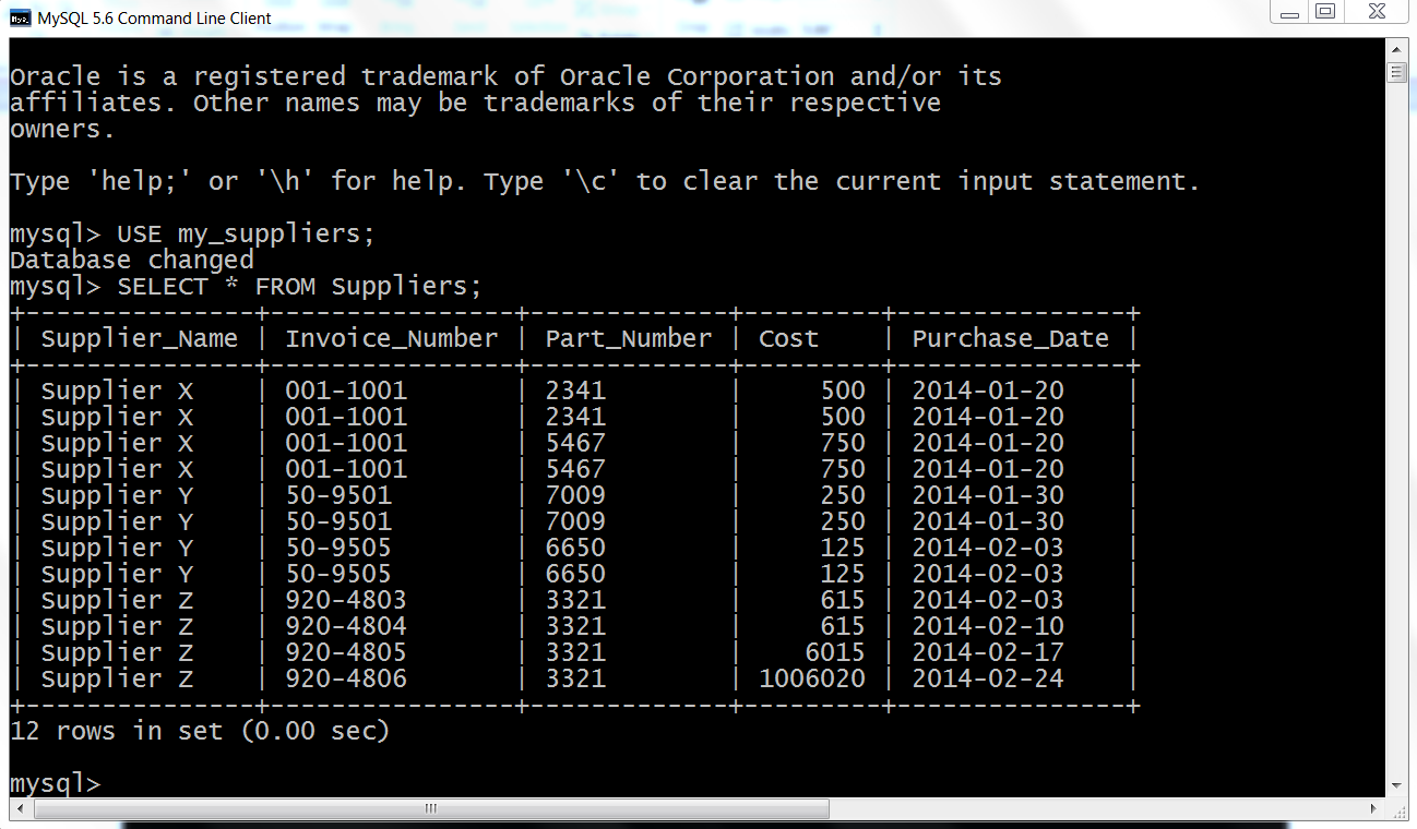
Now that we have a database table full of data, let’s learn how to query the database table and write the query output to a CSV output file with Python instead of printing the results to the screen.
Once you have data in a database table, one of the most common next steps is to query the table for a subset of data that is useful for an analysis or answers a business question. For example, you may be interested in the subset of customers who are providing the most profit, or you may be interested in the subset of expenses that exceed a particular threshold.
Let’s create a new Python script. The script will query the Suppliers database table for a specific set of records and then write the output to a CSV output file. In this case, we want to output all of the columns of data for records where the value in the Cost column is greater than 1,000.00. To begin, type the following code into a text editor and save the file as 5db_mysql_write_to_file.py:
#!/usr/bin/env python3importcsvimportMySQLdbimportsys# Path to and name of a CSV output fileoutput_file=sys.argv[1]# Connect to a MySQL databasecon=MySQLdb.connect(host='localhost',port=3306,db='my_suppliers',\user='root',passwd='my_password')c=con.cursor()# Create a file writer object and write the header rowfilewriter=csv.writer(open(output_file,'w',newline=''),delimiter=',')header=['Supplier Name','Invoice Number','Part Number','Cost','Purchase Date']filewriter.writerow(header)# Query the Suppliers table and write the output to a CSV filec.execute("""SELECT *FROM SuppliersWHERE Cost > 700.0;""")rows=c.fetchall()forrowinrows:filewriter.writerow(row)
The lines of code in this example are nearly a subset of the lines of code in the previous example, so I will emphasize the new lines.
Lines 2, 3, and 4 import the csv, MySQLdb, and sys modules, respectively, so we can use their methods to interact with a MySQL database and write query output to a CSV file.
Line 6 uses the sys module to read the path to and name of a file on the command line and assigns that value to the variable output_file.
Line 8 uses the MySQLdb module’s connect() method to connect to my_suppliers, the MySQL database we created earlier in this chapter. Line 10 creates a cursor that we can use to execute SQL statements against the Suppliers table in the my_suppliers database and to commit the changes to the database.
Line 12 uses the csv module’s writer() method to create a writer object called file_writer.
Line 13 creates a list variable called header that contains five strings that correspond to the column headings in the database table. Line 14 uses the filewriter’s writerow() method to write this list of strings, separated by commas, to the CSV-formatted output file. The database query will only output the data, not the column headings, so these lines of code ensure that the columns in our output file have column headings.
Lines 16 to 18 are the query that selects all of the columns for the subset of rows where the value in the Cost column is greater than 700.0. The query can flow over multiple lines because it is contained between triple double quotation marks. It is very useful to enclose your query in triple double quote so that you can format your query for readability.
Lines 19 to 21 are very similar to the lines of code in the previous example, except instead of printing the output to the Command Prompt/Terminal window, line 21 writes the output to a CSV-formatted output file.
Now that we have our Python script, let’s use our script to query specific data from our Suppliers database table and write the output to a CSV-formatted output file. To do so, type the following on the command line and then hit Enter:
python 5db_mysql_write_to_file.py output_files\5output.csv
You won’t see any output printed to the Command Prompt or Terminal window, but you can open the output file, 5output.csv, to review the results.
As you’ll see, the output file contains a header row with the names of the five columns, as well as the four rows in the database table where the value in the Cost column is greater than 700.0. Excel reformats the dates in the Purchase Date column to M/DD/YYYY, and the values in the Cost column do not contain commas or dollar signs, but it is easy to reformat these values if necessary.
Loading data into a database table and querying a database table are two common actions you take with database tables. Another common action is updating existing rows in a database table. The next example covers this situation, explaining how to update existing rows in a table.
The previous examples explained how to add rows to a MySQL database table at scale using a CSV input file and write the result of a SQL query to a CSV output file. But sometimes, instead of loading new data into a table or querying a table you need to update existing rows in a table.
Fortunately, we can reuse the technique of reading data from a CSV input file to update existing rows in a table. In fact, the technique of assembling a row of values for the SQL statement and then executing the SQL statement for every row of data in the CSV input file remains the same as in the earlier example. The SQL statement is what changes. It changes from an INSERT statement to an UPDATE statement.
Because we’re already familiar with how to use a CSV input file to load data into a database table, let’s learn how to use a CSV input file to update existing records in a MySQL database table. To do so, type the following code into a text editor and save the file as 6db_mysql_update_from_csv.py:
1#!/usr/bin/env python32importcsv3importMySQLdb4importsys5 6# Path to and name of a CSV input file7input_file=sys.argv[1]8# Connect to a MySQL database9con=MySQLdb.connect(host='localhost',port=3306,db='my_suppliers',\ 10user='root',passwd='my_password')11c=con.cursor()12 13# Read the CSV file and update the specific rows14file_reader=csv.reader(open(input_file,'r',newline=''),delimiter=',')15header=next(file_reader,None)16forrowinfile_reader:17data=[]18forcolumn_indexinrange(len(header)):19data.append(str(row[column_index]).strip())20(data)21c.execute("""UPDATE Suppliers SET Cost=%s, Purchase_Date=%s\22WHERE Supplier_Name=%s;""",data)23con.commit()24# Query the Suppliers table25c.execute("SELECT * FROM Suppliers")26rows=c.fetchall()27forrowinrows:28output=[]29forcolumn_indexinrange(len(row)):30output.append(str(row[column_index]))31(output)
All of the code in this example should look very familiar. Lines 2–4 import three of Python’s built-in modules so we can use their methods to read a CSV input file, interact with a MySQL database, and read command line input. Line 7 assigns the CSV input file to the variable input_file.
Line 10 makes a connection to the my_suppliers database with the same connection parameters we used in the previous examples, and line 12 creates a cursor object that can be used to execute SQL queries and commit changes to the database.
Lines 15–24 are nearly identical to the code in the first example in this chapter. The only significant difference is in line 22, where an UPDATE statement has replaced the previous INSERT statement. The UPDATE statement is where you have to specify which records and column attributes you want to update. In this case, we want to update the Cost and Purchase Date values for a specific set of Supplier Names. Like in the previous example, there should be as many placeholder %s as there are values in the query, and the order of the data in the CSV input file should be the same as the order of the attributes in the query. In this case, from left to right, the attributes in the query are Cost, Purchase_Date, and Supplier_Name; therefore, the columns from left to right in the CSV input file should be Cost, Purchase Date, and Supplier Name.
Finally, the code in lines 27–32 is basically identical to the same section of code in the earlier example. These lines of code fetch all of the rows in the Suppliers table and print each row to the Command Prompt or Terminal window, with a single space between column values.
Now all we need is a CSV input file that contains all of the data we need to update some of the records in our database table:
Open Excel.
Add the data in Figure 4-15.
Save the file as data_for_updating_mysql.csv.
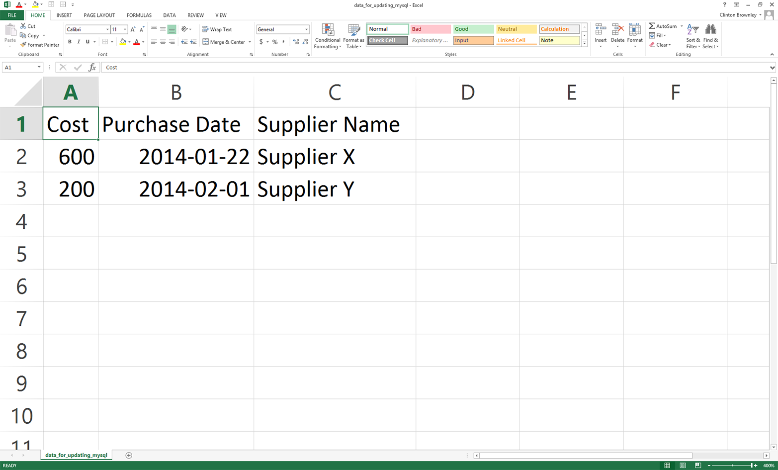
Now that we have our Python script and CSV input file, let’s use our script and input file to update specific records in our Suppliers database table. To do so, type the following on the command line and then hit Enter:
python 6db_mysql_update_from_csv.py data_for_updating_mysql.csv
On windows, you should see the output shown in Figure 4-16 printed to the Command Prompt window. The first two rows are the data in the CSV file, and the remaining rows are the data in the table after the records have been updated.
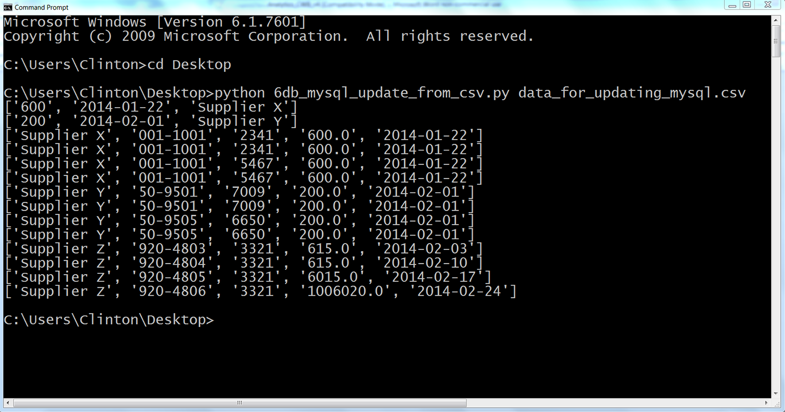
This output shows the two lists of values created for the two rows of data, excluding the header row, in the CSV input file. You can recognize the two lists because each list is enclosed in square brackets ([]) and the values in the lists are separated by commas. For Supplier X, the Cost value is 600 and the Purchase Date value is 2014-01-22. For Supplier Y, the Cost value is 200 and the Purchase Date value is 2014-02-01.
Beneath the two lists, the output also shows the 12 rows fetched from the database table after the updates were executed. Each row is printed on a separate line, and the values in each row are separated by single spaces. Recall that the original Cost and Purchase Date values for Supplier X were 500 and 750 and 2014-01-20, respectively. Similarly, the original Cost and Purchase Date values for Supplier Y were 250 and 125 and 2014-01-30 and 2013-02-03, respectively. As you can see in the output printed to the Command Prompt window, these values have been updated for Supplier X and Supplier Y to reflect the new values supplied in the CSV input file.
To confirm that the eight rows of data associated with Supplier X and Supplier Y have been updated in the MySQL database table, return to the MySQL command-line client, type the following, and then hit Enter:
SELECT * FROM Suppliers;
After you hit Enter, you should see a table that lists the columns in the Suppliers database table and the 12 rows of data in each of the columns, as in Figure 4-17. You can see that the eight rows associated with Supplier X and Supplier Y have been updated to reflect the data in the CSV input file.
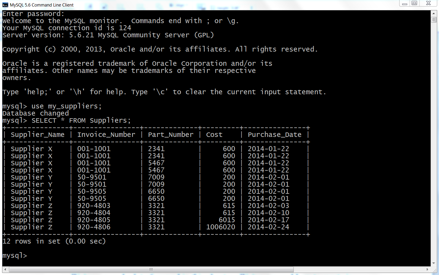
We’ve covered a lot of ground in this chapter. We discussed how to create in-memory and persistent databases with sqlite3 and interact with tables in those databases, and we saw how to create MySQL databases and tables, access MySQL databases and tables with Python, load data from a CSV file into a MySQL database table, update records in a MySQL database table with data from a CSV file, and write query output to a CSV output file. If you’ve followed along with the examples in this chapter, you have written six new Python scripts!
The best part about all of the work you have put into working through the examples in this chapter is that you are now well equipped to access data in databases, one of the most common data repositories in business. This chapter focused on the MySQL database system, but as we discussed at the beginning of this chapter, there are many other database systems used in business today. For example, you can learn about the PostgreSQL database system, and you can find information about a popular Python connection adapter for PostgreSQL at both the Psycopg and PyPI websites. Similarly, you can learn about the Oracle database system, and there is information about an Oracle connection adapter at SourceForge and PyPI. In addition, there is a popular Python SQL toolkit called SQLAlchemy that supports both Python 2 and 3 and includes adapters for SQLite, MySQL, PostgreSQL, Oracle, and several other database systems.
At this point, you’ve learned how to access, navigate, and process data in CSV files, Excel workbooks, and databases, three of the most common data sources in business. The next step is to explore a few applications to see how you can combine these new skills to accomplish specific tasks. First, we’ll discuss how to find a set of items in a large collection of files. The second application demonstrates how to calculate statistics for any number of categories in an input file. Finally, the third application demonstrates how to parse a text file and calculate statistics for any number of categories. After working through these examples, you should have an understanding of how you can combine the skills you’ve learned throughout the book to accomplish specific tasks.
Practice loading data from a CSV file into a database table by creating a new table, creating a new input file, and writing a new Python script that loads the input data into the table, either in SQLite3 or MySQL.
Practice querying a database table and writing the results to a CSV output file, either in SQLite3 or MySQL. Create a new Python script that has a new query to extract data from one of the tables you’ve created. Incorporate and modify the code from the MySQL script that demonstrates how to write to an output file to write a relevant header row and the data from your query.
Practice updating records in a database table with data from a CSV file, either in SQLite3 or MySQL. Create a new database table and load data into the table. Create a new CSV file with the data needed to update specific records in the table. Create a new Python script that updates specific records in your table with the data from the CSV file.
1 You can learn more about CRUD operations at http://en.wikipedia.org/wiki/Create,_read,_update_and_delete.
2 SQL injection attacks are malicious SQL statements that an attacker uses to obtain private information or damage data repositories and applications. You can learn more about SQL injection attacks at http://en.wikipedia.org/wiki/SQL_injection.
3 These packages are available at the Python Package Index.
Companies accumulate a lot of files on various aspects of their business. There may be historical files on suppliers, customers, internal operations, and other aspects of business. As we’ve already discussed, this data can be stored in flat, delimited files like CSV files, in Excel workbooks and spreadsheets, or in other storage systems. It is worthwhile to save these files because they provide data for analyses, they can help you track changes over time, and they provide supporting evidence.
But when you have a lot of historical files, it can be difficult to find the data you need. Imagine you have a combination of 300 Excel workbooks and 200 CSV files (you’ve used both file extensions interchangeably over the years) that contain data on supplies you’ve purchased over the past five years. You are now in a discussion with a supplier and you want to find some historical records that contain data that can inform your discussion.
Sure, you can open each file, look for the records you need, and copy and paste the records to a new file, but think about how painstaking, time consuming, and error prone the process will be. This is an excellent situation to use your new Python coding skills to automate the whole process to save time and reduce the number of errors.
In order to simulate searching through hundreds of Excel workbooks and CSV files in a folder of historical files, we need to create the folder of historical files and some Excel workbooks and CSV files. To do so:
Navigate to your Desktop.
Right-click on your Desktop.
Select New and then Folder to create a new folder on your Desktop.
Type “file_archive” as the name of the new folder.
Now you should have a new folder called file_archive on your Desktop (Figure 5-1).

Open Excel and add the data shown in Figure 5-2.
This CSV file has five columns: Item Number, Description, Supplier, Cost, and Date. You can see in the first column that only widgets have item numbers. There are separate records for widget service and maintenance, but service and maintenance records do not have item numbers.
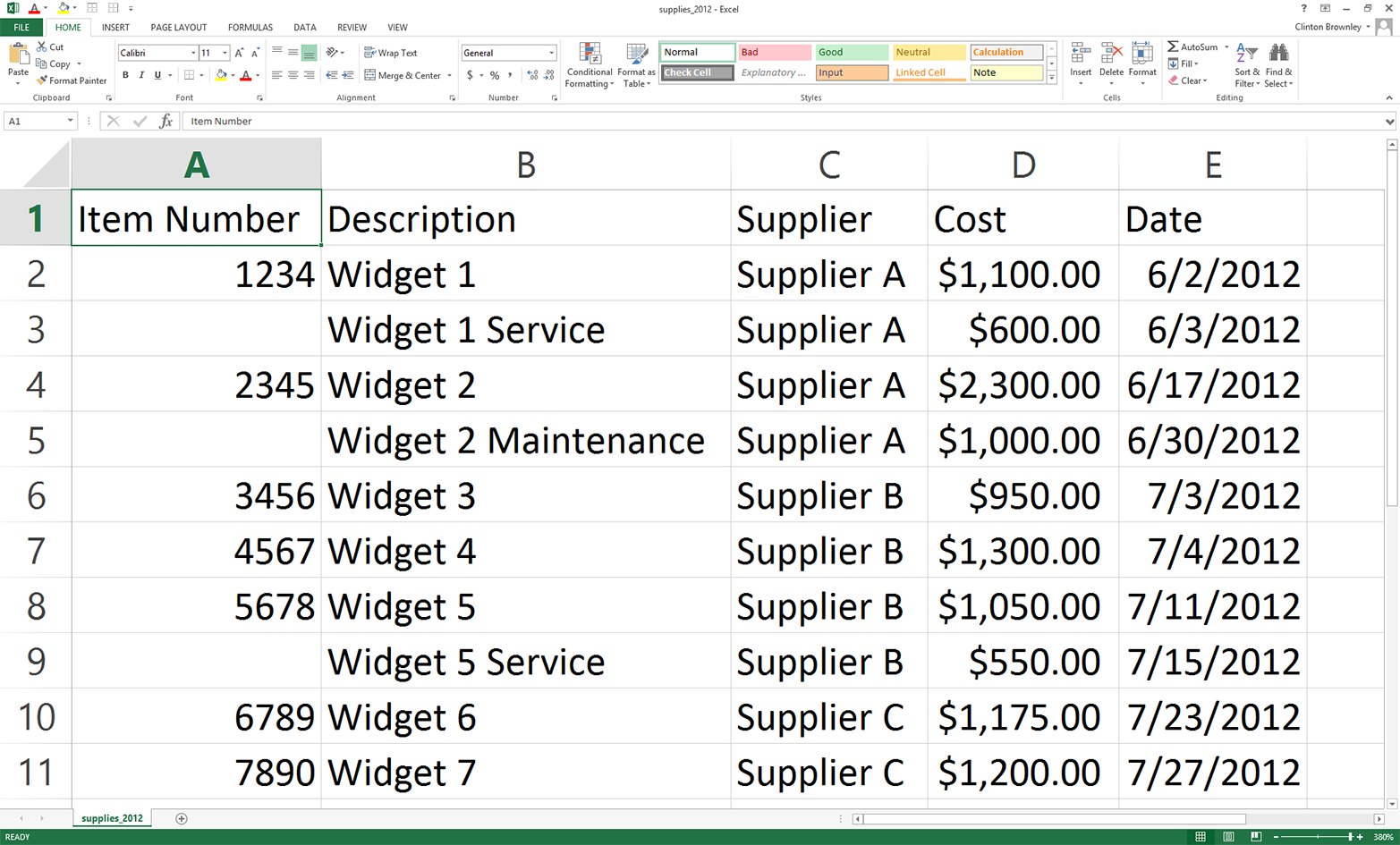
Save the file inside the file_archive folder as supplies_2012.csv.
OK, now we have a CSV file. Next, we need to create an Excel workbook. To do this quickly, let’s use the CSV file we created.
In supplies_2012, change the dates in the Date column to 2013 instead of 2012.
The worksheet should now look as shown in Figure 5-3. As you can see, only the dates have changed.
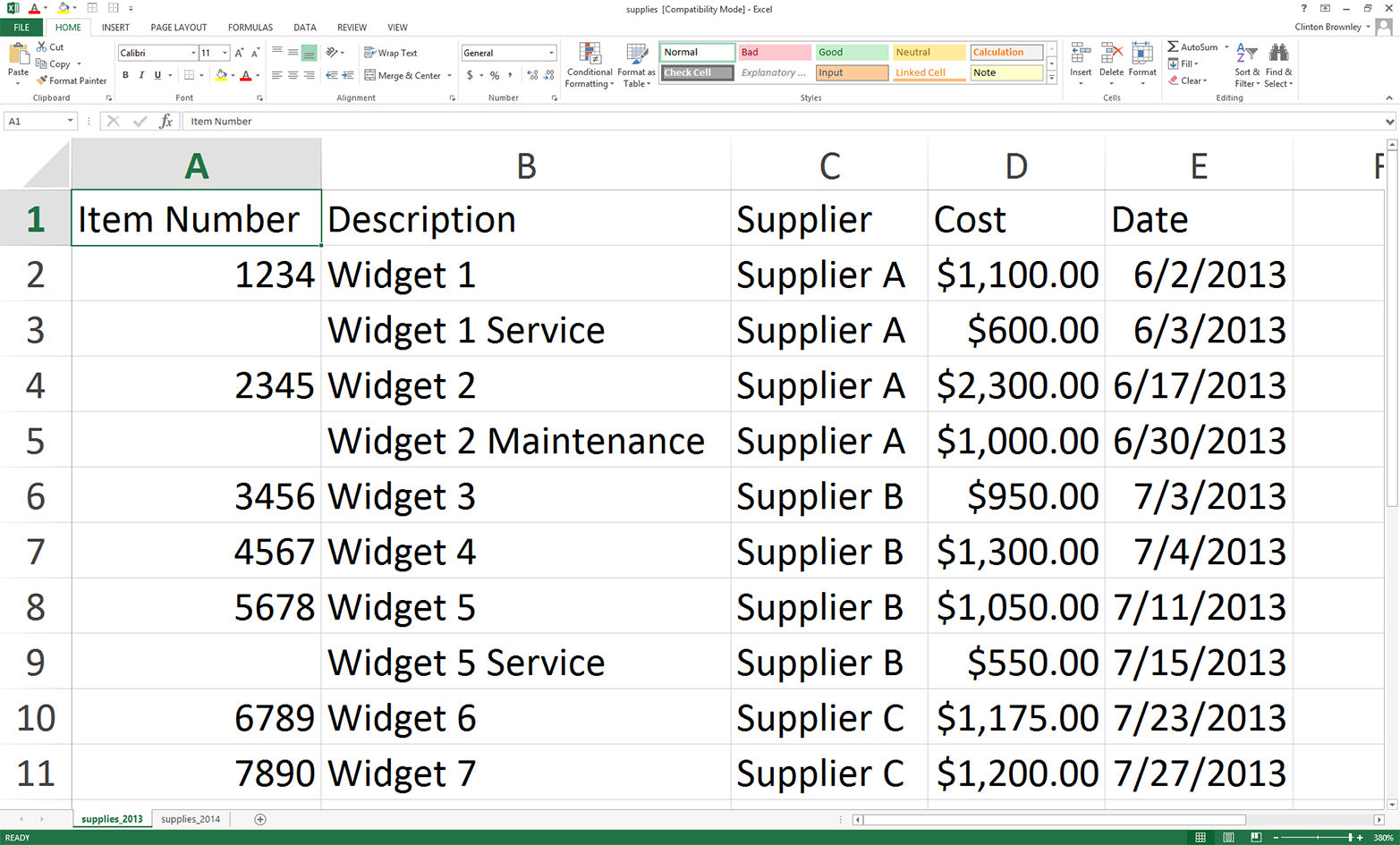
Change the name of the worksheet to supplies_2013.
To make this file a workbook with multiple worksheets, let’s add a new worksheet.
Add a new worksheet by clicking on the + button in the lower-left corner.
Name the new worksheet supplies_2014.
Copy and paste all of the data from the supplies_2013 worksheet to the supplies_2014 worksheet.
Change the dates in the Date column to 2014 instead of 2013.
The supplies_2014 worksheet should now look as shown in Figure 5-4.
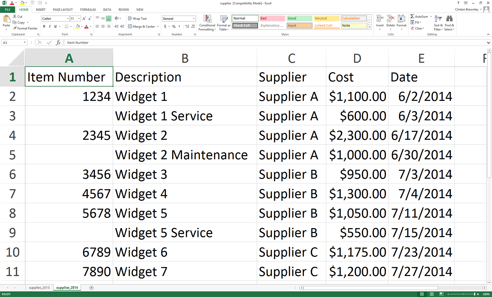
As you can see, only the dates have changed—that is, all of the data in the two worksheets is the same, except for the dates in the Date column.
Save the Excel file in the file_archive folder as supplies.xls.
As a final, optional step, if you can save the file in the Excel Workbook format (.xlsx), reopen the “Save As” dialog box and also save the file as supplies.xlsx.
You should now have three files saved in the file_archive folder:
A CSV file: supplies_2012.csv
An Excel file: supplies.xls
An Excel Workbook file (optional): supplies.xlsx
The example will still work if you could not create the optional .xlsx file, but you’ll have less output. These three files will serve as our set of accumulated historical files, but keep in mind that the code in this example scales to as many CSV and Excel files as your computer can handle.1 If you have hundreds or thousands of historical CSV or Excel files, you can still use the code in this example as a starting point for your specific search problem, and the code will scale.
Now that we have the folder and files we’re going to search in for the records we want, we need some way to identify the records we’re looking for. In this example, we’ll be searching for specific item numbers. If we were only looking for a few item numbers, we could hardcode them into the Python script as a list or tuple variable (e.g., items_to_look_for = ['1234', '2345']), but this method becomes burdensome or infeasible as the number of items to search for grows. Therefore, we’ll use the method we’ve been using to pass input data into a script and have the item numbers listed in a column in a CSV input file. This way, if you’re looking for a few dozen, hundred, or thousand item numbers, you can list them in a CSV input file and then read that input data into the Python script. This input method scales fairly well, especially compared to hardcoding the values into the Python script.
To list the item numbers that identify the records we’re looking for:
Open Excel and add the data shown in Figure 5-5.
Save the file as item_numbers_to_find.csv.
As you can see, the five item numbers we’re looking for are 1234, 2345, 4567, 6789, and 7890. They are listed in column A, with no header row. We could include a header row, but it’s unnecessary as we know which column to use and we know the meaning of the data. Plus, if we had a header row we’d have to add some code to process it and remove it because we’re presumably not looking for the header row value in the input files. If in the future another person or program supplies you with this list and it contains a header row, you’ve learned in earlier chapters how to remove it by reading it into a variable and then not using the variable. If you create the list yourself, it makes sense to not include a header row; doing so simplifies the code you need for data processing, and you can recall the meaning of the data based on the filename and the name of the project folder the file is in.
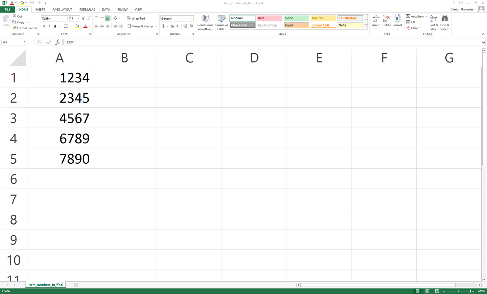
At this point, we understand the search task and we have the folder and files we need to carry out the example. To recap, the task is to search in the file_archive folder for files that contain any of the item numbers we’re looking for and, when an item number is found, to write the entire row that contains the item number should be written to an output file. That way, we have all of the historical information associated with the item number available for our discussion with the supplier. We have three historical files in which to search: a CSV file, an Excel file (.xls), and an Excel Workbook file (.xlsx). These three files keep the setup for this example to a minimum, but the code in the script scales and can handle as many input files as your computer can handle. We also have a separate CSV file that contains the item numbers we want to find. We can list hundreds, thousands, or more item numbers in this file, so this input method helps us scale the search as well.
Now that we’ve created the file_archive folder and all of the input files, all we need to do is write some Python code to carry out our search task for us. To do so, type the following code into a text editor and save the file as 1search_for_items_write_found.py:
1#!/usr/bin/env python32importcsv3importglob4importos5importsys6fromdatetimeimportdate7fromxlrdimportopen_workbook,xldate_as_tuple8item_numbers_file=sys.argv[1]9path_to_folder=sys.argv[2]10output_file=sys.argv[3]11item_numbers_to_find=[]12withopen(item_numbers_file,'r',newline='')asitem_numbers_csv_file:13filereader=csv.reader(item_numbers_csv_file)14forrowinfilereader:15item_numbers_to_find.append(row[0])16#print(item_numbers_to_find)17filewriter=csv.writer(open(output_file,'a',newline=''))18file_counter=019line_counter=020count_of_item_numbers=021forinput_fileinglob.glob(os.path.join(path_to_folder,'*.*')):22file_counter+=123ifinput_file.split('.')[1]=='csv':24withopen(input_file,'r',newline='')ascsv_in_file:25filereader=csv.reader(csv_in_file)26header=next(filereader)27forrowinfilereader:28row_of_output=[]29forcolumninrange(len(header)):30ifcolumn==3:31cell_value=str(row[column]).lstrip('$').\ 32replace(',','').strip()33row_of_output.append(cell_value)34else:35cell_value=str(row[column]).strip()36row_of_output.append(cell_value)37row_of_output.append(os.path.basename(input_file))38ifrow[0]initem_numbers_to_find:39filewriter.writerow(row_of_output)40count_of_item_numbers+=141line_counter+=142elifinput_file.split('.')[1]=='xls'or\ 43input_file.split('.')[1]=='xlsx':44workbook=open_workbook(input_file)45forworksheetinworkbook.sheets():46try:47header=worksheet.row_values(0)48exceptIndexError:49pass50forrowinrange(1,worksheet.nrows):51row_of_output=[]52forcolumninrange(len(header)):53ifworksheet.cell_type(row,column)==3:54cell_value=\ 55xldate_as_tuple(worksheet.cell(row,column)\ 56.value,workbook.datemode)57cell_value=str(date(*cell_value[0:3])).strip()58row_of_output.append(cell_value)59else:60cell_value=\ 61str(worksheet.cell_value(row,column)).strip()62row_of_output.append(cell_value)63row_of_output.append(os.path.basename(input_file))64row_of_output.append(worksheet.name)65ifstr(worksheet.cell(row,0).value).split('.')[0].strip()\ 66initem_numbers_to_find:67filewriter.writerow(row_of_output)68count_of_item_numbers+=169line_counter+=170('Number of files:',file_counter)71('Number of lines:',line_counter)72('Number of item numbers:',count_of_item_numbers)
This is a longer script than the ones we wrote in the previous chapter, but if you’ve completed the examples in the preceding chapters then all of the code in this script should look familiar. Lines 2–7 import modules and methods we need to read and manipulate the input data. We import the csv, glob, os, string, and sys modules to read and write CSV files, read multiple files in a folder, find files in a particular path, manipulate string variables, and enter input on the command line, respectively. We import the datetime module’s date method and the xlrd module’s xldate_as_tuple method, as we did in Chapter 3, to ensure that any dates we extract from the input files have a particular format in the output file.
Lines 8, 9, and 10 take the three pieces of input we supply on the command line—the path to and name of the CSV file that contains the item numbers we want to find, the path to the file_archive folder that contains the files in which we want to search, and the path to and name of the CSV output file that will contain rows of information associated with the item numbers found in the historical files—and assign the inputs to three separate variables (item_numbers_file, path_to_folder, and output_file, respectively).
To use the item numbers that we want to find in the code, we need to transfer them from the CSV input file into a suitable data structure like a list. Lines 11–15 accomplish this transfer for us. Line 11 creates an empty list called item_numbers_to_find. Lines 12 and 13 use the csv module’s reader() method to open the CSV input file and create a filereader object for reading the data in the file. Line 14 creates a for loop for looping over all of the rows in the input file. Line 14 uses the list’s append() method to add values to the list we created in line 11. The values added to our list come from the first column, row[0], in the CSV input file. If you want to see the item numbers appended into the list printed to your screen when you run the script, you can uncomment the print statement in line 16.
Line 17 uses the csv module’s writer() method to open a CSV output file in append ('a') mode and creates a filewriter object for writing data to the output file.
Lines 18,19, and 20 create three counter variables to keep track of (a) the number of historical files read into the script, (b) the number of rows read across all of the input files and worksheets, and (c) the number of rows where the item number in the row is one of the item numbers we’re looking for. All three counter variables are initialized to zero.
Line 21 is the outer for loop that loops over all of the input files in the historical files folder. This line uses the os.path.join() function and the glob.glob() function to find all of the files in the file_archive folder that match a specific pattern. The path to the file_archive folder is contained in the variable path_to_folder, which we supply on the command line. The os.path.join() function joins this folder path with all of the names of files in the folder that match the specific pattern expanded by the glob.glob() function. Here, we use the pattern '*.*' to match any filename that ends with any file extension. In this case, because we created the input folder and files, we know the only file extensions in the folder are .csv, .xls, and .xlsx. If instead you only wanted to search in CSV files, then you could use '*.csv'; and if you only wanted to search in .xls or .xlsx files, then you could use '*.xls*'. This a for loop, so the rest of the syntax on this line should look familiar. input_file is a placeholder name for each of the files in the list created by the glob.glob() function.
Line 22 adds one to the file_counter variable for each input file read into the script. After all of the input files have been read into the script, file_counter will contain the total number of files read in.
Line 23 is an if statement that initiates a block of code associated with CSV files. The counterpart of this line is the elif statement in line 42 that initiates a block of code associated with .xls and .xlsx files. Line 23 uses the string module’s split() method to split the path to each input file at the period (.) in the path. For example, the path to the CSV input file is file_archive\supplies_2012.csv. Once this string is split on the period, everything before the period has index [0] and everything after the period has index [1]. This line tests whether the string after the period, with index [1], is csv, which is true for the CSV input file. Therefore, lines 24 to 41 are executed for the CSV input file.
Lines 24 and 25 are familiar. They use the csv module’s reader() method to open the CSV input file and create a filereader object for reading the data in the file.
Line 26 uses the next() method to read the first row of data in the input file, the header row, into a variable called header.
Line 27 creates a for loop for looping through the remaining rows of data in the CSV file. For each of these rows, if the row contains one of the item numbers we’re looking for, then we need to assemble a row of output to write to the output file. To prepare for assembling the row of output, line 28 creates an empty list variable called row_of_output.
Line 29 creates a for loop for looping over each of the columns in a given row in the input file. The line uses the range() and len() functions to create a list of indices associated with the columns in the CSV input file. Because the input file contains five columns, the column variable ranges from 0 to 4.
Lines 30–36 contain an if-else statement that makes it possible to perform different actions on the values in different columns. The if block acts on the column with index 3, which is the fourth column, Cost. For this column, the lstrip() method strips the dollar sign from the lefthand side of the string; the replace() method replaces the comma in the string with no space (effectively deleting the comma); and the strip() method strips any spaces, tabs, and newline characters from the ends of the string. After all of these manipulations, the value is appended into the list; row_of_output in line 37.
The else block acts on the values in all of the other columns. For these values, the strip() method strips any spaces, tabs, and newline characters from the ends of the string, and then the value is appended into the list row_of_output in line 36.
Line 37 appends the basename of the input filename into the list row_of_output. For the CSV input file, the variable input_file contains the string file_archive\supplies_2012.csv. os.path.basename ensures that only supplies_2012.csv is appended into the list row_of_output.
At this point, the first row of data in the CSV input file has been read into the script and each of the column values in the row have been manipulated and then appended into the list row_of_output. Now it is time to test whether the item number in the row is one of the item numbers we want to find. Line 38 carries out this evaluation. The line tests whether the value in the first column in the row, the item number, is in the list of item numbers we want to find, contained in the list variable called item_numbers_to_find. If the item number is one of the item numbers we want to find, then we use the filewriter’s writerow() method in line 39 to write the row of output to our CSV output file. We also add one to the count_of_item_numbers variable in line 40 to keep track of the number of item numbers we found in all of the input files.
Finally, before moving on to the next row of data in the CSV input file, we add one to the line_counter variable in line 41 to keep track of the number of rows of data we found in all of the input files.
The next block of code, in lines 42 through 69 is very similar to the preceding block of code except that it manipulates Excel files (.xls and .xlsx) instead of CSV files. Because the logic in this “Excel” block is the same as the logic in the “CSV” block—the only difference is the syntax for Excel files instead of CSV files—I won’t go into as much detail on every line of code.
Line 42 is an elif statement that initiates a block of code associated with .xls and .xlsx Excel files. Line 42 uses an “or” condition to test whether the file extension is .xls or .xlsx. Therefore, lines 43 to 69 are executed for the .xls and .xlsx Excel input files.
Line 43 uses the xlrd module’s open_workbook() method to open an Excel workbook and assigns its contents to the variable workbook.
Line 44 creates a for loop for looping over all of the worksheets in a workbook. For each worksheet, lines 45 to 48 try to read the first row in the worksheet—the header row—into the variable header. If there is an IndexError, meaning the sequence subscript is out of range, then the Python keyword pass executes and does nothing, and the code continues to line 49.
Line 49 creates a for loop for looping over the remaining data rows in the Excel input file. The range begins at 1 instead of 0 to start at the second row in the worksheet (effectively skipping the header row).
The remaining lines of code in this “Excel” block are basically identical to the code in the “CSV” block, except that they use Excel parsing syntax instead of CSV parsing syntax. The if block acts on the column where the cell type evaluates to 3, which is the column that contains numbers that represent dates. This block uses the xlrd module’s xldate_as_tuple() method and the datetime module’s date() method to make sure the date value in this column retains its date formatting in the output file. Once the value is converted into a text string with date formatting, the strip() method strips any spaces, tabs, and newline characters from the ends of the string and then the list’s append() method appends the value into the list, row_of_output, in line 57.
The else block acts on the values in all of the other columns. For each of these values, the strip() method strips any spaces, tabs, and newline characters from the ends of the string and then the value is appended into the list row_of_output, in line 61.
Line 62 appends the basename of the input filename into the list row_of_output. Unlike CSV files, Excel files can contain multiple worksheets. Therefore, line 63 also appends the name of the worksheet into the list. This additional information for Excel files makes it even easier to see where the script found the item number.
Lines 64–68 are similar to the lines of code for CSV files. Line 64 tests whether the value in the first column in the row, the item number, is in the list of item numbers we want to find, contained in the list variable called item_numbers_to_find. If the item number is one of the item numbers we want to find, then we use the filewriter’s writerow() method in line 66 to write the row of output to our CSV output file. We also add one to the count_of_item_numbers variable in line 67 to keep track of the number of item numbers we found in all of the input files.
Finally, before moving on to the next row of data in the Excel worksheet, we add one to the line_counter variable in line 68 to keep track of the number of rows of data we found in all of the input files.
Lines 69, 70, and 71 are print statements that print summary information to the Command Prompt or Terminal window once the script is finished processing all of the input files. Line 69 prints the number of files processed. Line 70 prints the number of lines read across all of the input files and worksheets. Line 71 prints the number of rows where we found an item number that we were looking for. This count can include duplicates. For example, if item number “1234” appears twice in a single file or once in two separate files, then item number “1234” is counted twice in the value printed to the Command Prompt/Terminal window by this line of code.
Now that we have our Python script, let’s use our script to find specific rows of data in a set of historical files and write the output to a CSV-formatted output file. To do so, type the following on the command line, and then hit Enter:
python 1search_for_items_write_found.py item_numbers_to_find.csv file_archive\ output_files\1app_output.csv
On Windows, you should see the output shown in Figure 5-6 printed to the Command Prompt window.
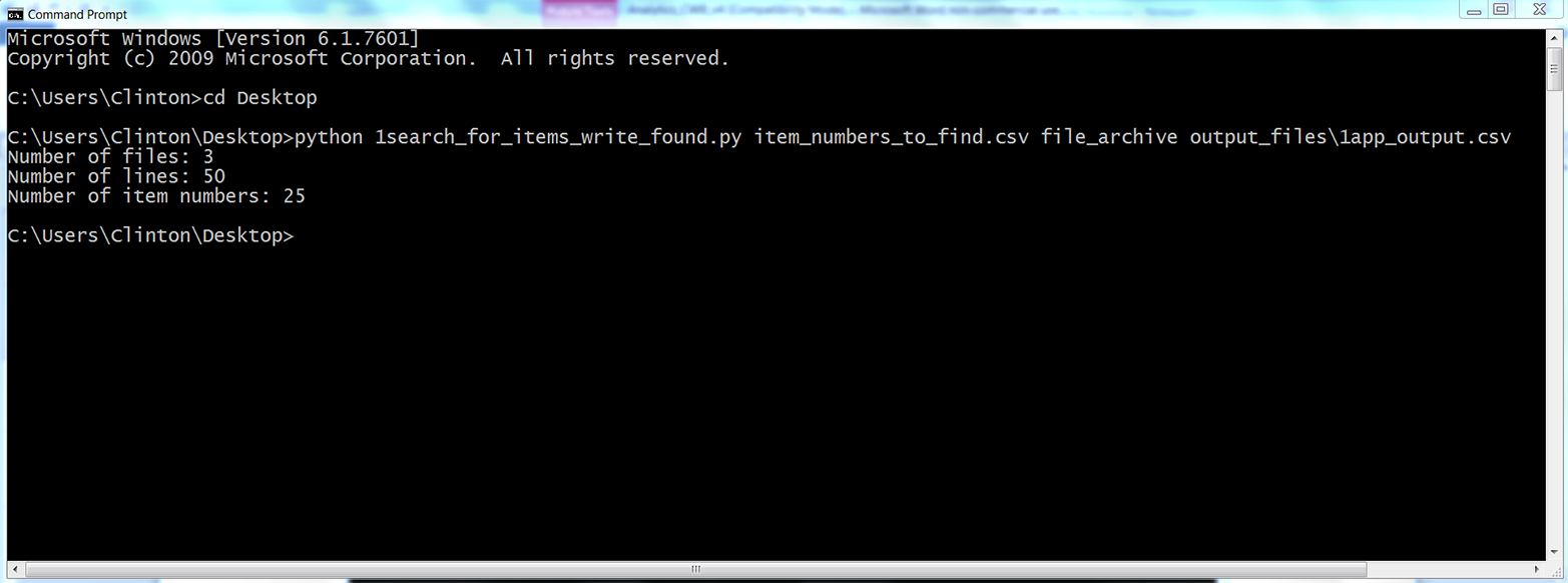
As you can see from the output printed to the Command Prompt window, the script read three input files, read 50 rows of data in the input files, and found 25 rows of data associated with the item numbers we wanted to find. This output doesn’t show how many of the item numbers were found or how many copies of each of the item numbers were found. However, that is why we wrote the output to a CSV output file.
To view the output, open the output file named 1app_output.csv. The contents should look as shown in Figure 5-7.
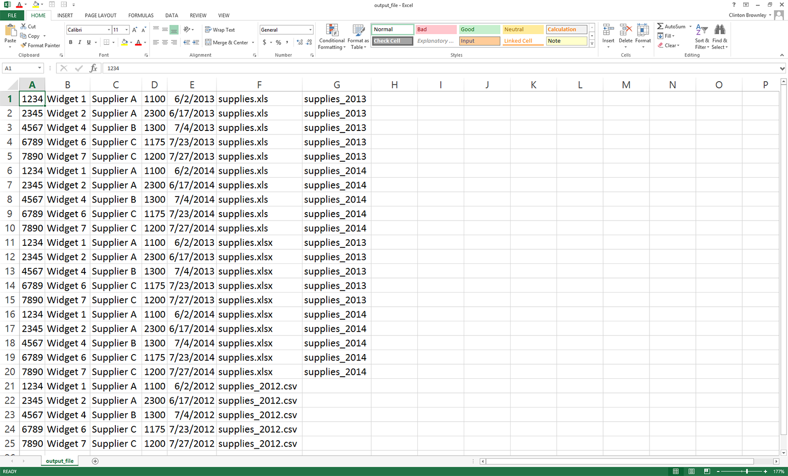
These records are the rows in the three input files that have item numbers matching those listed in the CSV file. The second-to-last column lists the names of the files where the data is found. The last column lists the names of the worksheets where the data is found in the two Excel workbooks.
As you can see from the contents of this output file, we found 25 rows of data associated with the item numbers we wanted to find. This output is consistent with the “25” that was printed to the Command Prompt window. Specifically, we found each of the five item numbers we wanted to find five times across all of the input files. For example, item number “1234” was found twice in the .xls file (once in the supplies_2013 worksheet and once in the supplies_2014 worksheet), twice in the .xlsx file (once in the supplies_2013 worksheet and once in the supplies_2014 worksheet), and once in the CSV input file.
Compared to the rows that came from the CSV input file, the rows of output that came from the Excel workbooks have an additional column (i.e., the name of the worksheet in which the row of data was found). The costs in the fourth column only include the dollar portion of the cost amount from the input files. Finally, the dates in the fifth column are formatted consistently across the CSV and Excel input files.
This application combined several of the techniques we learned in earlier chapters to tackle a common, real-world problem. Business analysts often run into the problem of needing to assemble historical data spread across multiple files and file types into a single dataset. In many cases, there are dozens, hundreds, or thousands of historical files and the thought of having to search for and extract specific data from these files is daunting.
In this section, we demonstrated a scalable way to extract specific records from a set of historical records. To keep the setup to a minimum, the example only included a short list of item numbers and three historical records. However, the method scales well, so you can use it to search for a longer list of items and in a much larger collection of files.
Now that we’ve tackled the problem of searching for specific records in a large collection of historical files, let’s turn to the problem of calculating a statistic for an unknown number of categories. This objective may sound a bit abstract right now, but let’s turn to the next section to learn more about this problem and how to tackle it.
Many business analyses involve calculating a statistic for an unknown number of categories in a specific period of time. For example, let’s say you sell five different products and you want to calculate the total sales by product category for all of your customers in a specific year. Because your customers have different tastes and preferences, they have purchased different products throughout the year. Some of your customers have purchased all five of your products; others have only purchased one of your products. Given your customers’ purchasing habits, the number of product categories associated with each customer differs across customers.
To make it easy, you could associate all five product categories with each of your customers, initiate total sales for all of the product categories at zero, and only increase the total sales amounts for the products each customer has actually purchased. However, we already know that many customers have only purchased one or two products, and you’re only interested in the total sales for the products that customers have actually purchased. Associating all five product categories with all of your customers is excessive, distracting, and wasteful of memory, computing resources, and storage space. For these reasons, it makes sense to only capture the data you need—for each customer, the products they purchased and the total sales in each of the product categories.
As another example, imagine that your customers progress through different product or service packages over time. For example, you supply a Bronze package, a Silver package, and a Gold package. Some customers buy the Bronze package first, some buy the Silver package first, and some buy the Gold package first. For those customers who buy the Bronze or Silver package first, they tend to progress to higher-value packages over time.
You are interested in calculating the total amount of time, perhaps in months, that your customers have spent in each of the package categories they’ve purchased. For example, if one of your customers, Tony Shephard, purchased the Bronze package on 2/15/2014, purchased the Silver package on 6/15/2014, and purchased the Gold package on 9/15/2014, then the output for Tony Shepard would be “Bronze package : 4 months”; “Silver package : 3 months”; and “Gold package: the difference between today’s date and 9/15/2014”. If a different customer, Mollie Adler, has only purchased the Silver and Gold packages, then the output for Mollie Adler would not include any information on the Bronze package.
If the dataset on your customers is small enough, then you could open the file, calculate the differences between the dates, and then aggregate them by package category and customer name. However, this manual approach would be time consuming and error prone. And what happens if the file is too large to open? This application is an excellent opportunity to use Python. Python can handle files that are too large to open, it performs the calculations quickly, and it reduces the chance of human errors.
In order to perform calculations on a dataset of customer package purchases, we need to create a CSV file with the data:
Open Excel and add the data shown in Figure 5-8.
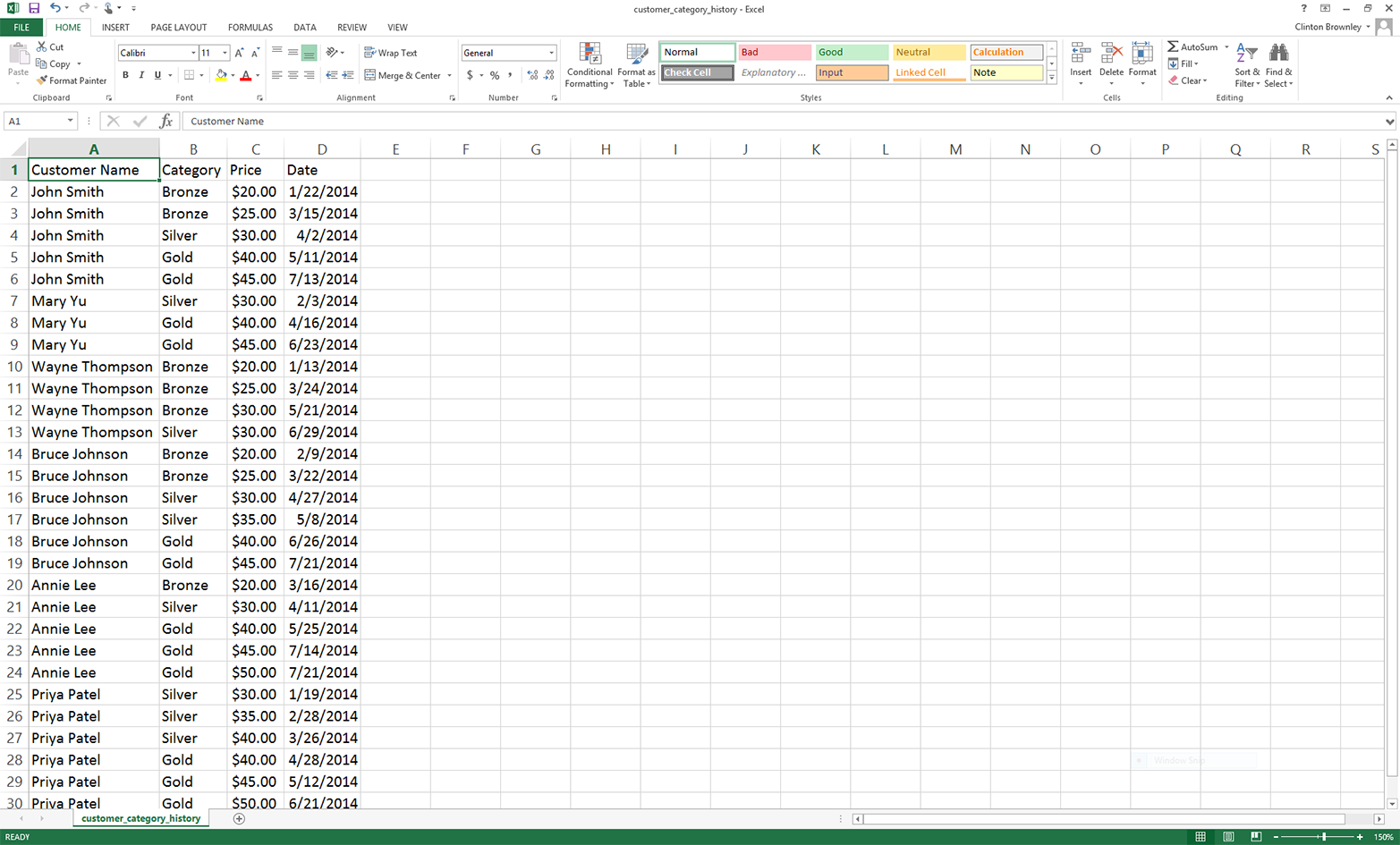
Save the file as customer_category_history.csv.
As you can see, this dataset includes four columns: Customer Name, Category, Price, and Date. It includes six customers: John Smith, Mary Yu, Wayne Thompson, Bruce Johnson, Annie Lee, and Priya Patel. It includes three package categories: Bronze, Silver, and Gold. The data is arranged by Customer Name and then by Date, ascending.
Now that we have our dataset on the packages our customers have purchased over the past year and the dates on which the packages were purchased or renewed, all we need to do is write some Python code to carry out our binning and calculation tasks for us.
To do so, type the following code into a text editor and save the file as 2calculate_statistic_by_category.py:
1#!/usr/bin/env python32importcsv3importsys4fromdatetimeimportdate,datetime5 6defdate_diff(date1,date2):7try:8diff=str(datetime.strptime(date1,'%m/%d/%Y')-\ 9datetime.strptime(date2,'%m/%d/%Y')).split()[0]10except:11diff=012ifdiff=='0:00:00':13diff=014returndiff15input_file=sys.argv[1]16output_file=sys.argv[2]17packages={}18previous_name='N/A'19previous_package='N/A'20previous_package_date='N/A'21first_row=True22today=date.today().strftime('%m/%d/%Y')23withopen(input_file,'r',newline='')asinput_csv_file:24filereader=csv.reader(input_csv_file)25header=next(filereader)26forrowinfilereader:27current_name=row[0]28current_package=row[1]29current_package_date=row[3]30ifcurrent_namenotinpackages:31packages[current_name]={}32ifcurrent_packagenotinpackages[current_name]:33packages[current_name][current_package]=034ifcurrent_name!=previous_name:35iffirst_row:36first_row=False37else:38diff=date_diff(today,previous_package_date)39ifprevious_packagenotinpackages[previous_name]:40packages[previous_name][previous_package]=int(diff)41else:42packages[previous_name][previous_package]+=int(diff)43else:44diff=date_diff(current_package_date,previous_package_date)45packages[previous_name][previous_package]+=int(diff)46previous_name=current_name47previous_package=current_package48previous_package_date=current_package_date49header=['Customer Name','Category','Total Time (in Days)']50withopen(output_file,'w',newline='')asoutput_csv_file:51filewriter=csv.writer(output_csv_file)52filewriter.writerow(header)53forcustomer_name,customer_name_valueinpackages.items():54forpackage_category,package_category_value\ 55inpackages[customer_name].items():56row_of_output=[]57(customer_name,package_category,package_category_value)58row_of_output.append(customer_name)59row_of_output.append(package_category)60row_of_output.append(package_category_value)61filewriter.writerow(row_of_output)
The code in this script accomplishes the calculation task, but it is also interesting and educational—it is the first example in this book to use Python’s dictionary data structure to organize and store our results. In fact, the example in this script is more complicated than a simple dictionary because it involves a nested dictionary, a dictionary within a dictionary. This example shows how convenient it can be to create a dictionary and to fill it with key-value pairs. In this example, the outer dictionary is called packages. The outer key is the customer’s name. The value associated with this key is another dictionary, where the key is the name of the package category and the value is an integer that captures the number of days the customer has had the specific package. Dictionaries are handy data structures to understand, because many data sources and analyses lend themselves to the key-value pair structure. As you’ll recall from Chapter 1, dictionaries are created with curly braces ({}), the keys in a dictionary are unique strings, the keys and values in a key-value pair are separated by colons, and each of the key-value pairs are separated by commas—for example, costs = {'people': 3640, 'hardware': 3975}.
In addition, this script demonstrates how to handle the first row of data about a particular category differently from all of the remaining rows about that category in order to calculate statistics based on differences between the rows. For example, in the script, all of the code in the outer if statement, if current_name != previous_name, is only executed for the first row of data about a new customer. All of the remaining rows about the customer enter into the outer else statement.
Finally, this script demonstrates how to define and use a user-defined function. The function in this script, date_diff, calculates and returns the amount of time in days between two dates. The function is defined in lines 6–14, and is used in lines 40 and 47. If we didn’t define a function, the code in the function would have to be repeated twice in the script, first at line 38 and again at line 44. By defining a function, you only have to write the code once, you reduce the number of lines of code in the script, and you simplify the code that appears in lines 40 and 47. As mentioned in Chapter 1, whenever you notice that you are repeating code in your script, consider bundling the code into a function and using the function to simplify and shorten the code in your script.
Now that we have covered some of the notable aspects of the script, let’s discuss specific lines of code. Lines 2–5 import modules and methods we need to read and manipulate the input data. We import the csv, datetime, string, and sys modules to read and write CSV files, manipulate date variables, manipulate string variables, and enter input on the command line, respectively. From the datetime module, we import the date and datetime methods to access today’s date and calculate differences between dates.
Lines 6–14 define the user-defined date_diff function. Line 6 contains the definition statement, which names the function and shows that the function takes two values, date1 and date2, as arguments to the function. Lines 7–11 contain a try-except error handling statement. The try block attempts to create datetime objects from date strings with datetime.strptime(), subtract the second date from the first date, convert the result of the subtraction into a string with str(), split the resulting string on whitespace with split(), and finally retain the leftmost portion of the split string (the string with index [0]) and assign it to the variable diff. The except block executes if the try block encounters any errors. If that happens, the except block sets diff to the integer zero. Similarly, lines 12 and 13 are an if statement that handles the situation when the two dates being processed are equal and therefore the difference between the dates is zero, formatted as '0:00:00'. If the difference evaluates to zero (note the two equals signs), then the if statement sets diff to the integer zero. Finally, in line 14 the function returns the integer value contained in the variable diff.
Lines 15 and 16 take the two pieces of input we supply on the command line—the path to and name of the CSV input file that contains our customer data, and the path to and name of the CSV output file that will contain rows of information associated with our customers and how long they’ve had particular packages—and assign the inputs to two separate variables (input_file and output_file, respectively.)
Line 17 creates an empty dictionary called packages that will contain the information we want to retain. Lines 18, 19, and 20 create three variables, previous_name, previous_package, and previous_package_date, and assign each of them the string value 'N/A'. We assign the value 'N/A' to these variables assuming the string 'N/A' does not appear anywhere in the three columns of customer names, package categories, or package dates in the input file. If you plan to modify this code for your own analysis and the column you’re using for your dictionary keys includes the string 'N/A', then change 'N/A' to a different string that doesn’t appear in your column in your input file—'QQQQQ' or something equally distinctive yet meaningless works.
Line 21 creates a Boolean variable called first_row and assigns it the value, True. We use this variable to determine whether we’re processing the first row of data in the input file. If we are processing the first row of data, then we process it with one block of code. If we’re not processing the first row, then we use another block of code.
Line 22 creates a variable called today that contains today’s date, formatted as %m/%d/%Y. With this format, a date like October 21, 2014 appears as 10/21/2014.
Lines 23 and 24 use a with statement and the csv module’s reader method to open the CSV input file and create a filereader object for reading the data in the file. Line 25 uses the next method on the filereader object to read the first row from the input file and assigns the list of values to the variable header.
Line 26 creates a for loop for looping over all of the remaining data rows in the input file. Line 27 captures the value in the first column, row[0], and assigns it to the variable current_name. Line 28 captures the value in the second column, row[1], and assigns it to the variable current_package. Line 29 captures the value in the fourth column, row[3], and assigns it to the variable current_package_date. The first data row contains the values John Smith, Bronze, and 1/22/2014, so these are the values assigned to current_name, current_package, and current_package_date, respectively.
Line 30 creates an if statement to test whether the value in the variable current_name is not already a key in the packages dictionary. If it is not, then line 31 adds the value in current_name as a key in the packages dictionary and sets the value associated with the key as an empty dictionary. These two lines serve to populate the packages dictionary with its collection of key-value pairs.
Similarly, line 32 creates an if statement to test whether the value in the variable current_package is not already a key in the inner dictionary associated with the customer name contained in the variable current_name. If it is not, then line 33 adds the value in current_package as a key in the inner dictionary and sets the value associated with the key as the integer zero. These two lines serve to populate the key-value pairs in the inner dictionary associated with each customer name.
For example, in line 31, John Smith becomes a key in the packages dictionary, and the associated value is an empty dictionary. In line 33, the first package category associated with John Smith (i.e., Bronze), becomes a key in the inner dictionary and the value associated with Bronze is initialized to zero. At this point, the packages dictionary looks like: {'John Smith': {'Bronze': 0}}.
Line 34 creates an if statement to test whether the value in the variable current_name does not equal the value in the variable previous_name. The first time we reach this line in the script, the value in current_name is the first customer name in our input file (i.e., John Smith). The value in previous_name is 'N/A'. Because John Smith doesn’t equal 'N/A', we enter the if statement.
Line 35 creates an if statement to test whether the code is processing the first row of data in the input file. Because the variable first_row currently has the value True, line 35 executes line 36, which assigns the variable first_row the value False.
Next, the script moves on to lines, 46, 47, and 48 to assign the values in the three variables current_name, current_package, and current_package_date to the three variables previous_name, previous_package, and previous_package_date, respectively. Therefore, previous_name now contains the value John Smith, previous_package now contains the value Bronze, and previous_package_date now contains the value 1/22/2014.
At this point, the script has finished processing the first row of data in the input file, so the script returns to line 26 to process the next row of data in the file. For this data row, lines 27, 28, and 29 assign the values in the first, second, and fourth columns in the row to the variables current_name, current_package, and current_package_date, respectively. Because the second row of data contains the values John Smith, Bronze, and 3/15/2014, these are now the values contained in current_name, current_package, and current_package_date.
Line 30 once again tests whether the value in the variable current_name is not already a key in the packages dictionary. Because John Smith is already a key in the dictionary, line 31 is not executed. Similarly, line 32 once again tests whether the value in the variable current_package is not already a key in the inner dictionary. Bronze is already a key in the inner dictionary, so line 33 is not executed.
Next, line 34 tests whether the value in current_name is not equal to the value in previous_name. The value in current_name is John Smith and the value in previous_name is also John Smith. Because the values in the two variables are equal, lines 35 to 42 are skipped and we move on to the else block that starts at line 43.
Line 44 uses the user-defined date_diff function to subtract the value in previous_package_date from the value in current_package_date and assigns the value (in days) to the variable diff. We’re processing the second data row in the input file, so the value in current_package_date is 3/15/2014. In the previous loop we assigned the value 1/22/2014 to the variable previous_package_date. Therefore, the value in diff is 3/15/2014 minus 1/22/2014, or 52 days.
Line 45 increments the amount of time a specific customer has had a specific package by the value in diff. For example, this time through the loop the value in previous_name is John Smith and the value in previous_package is Bronze. Therefore, we increment the amount of time John Smith has had the Bronze package from zero to 52 days. At this point, the packages dictionary looks like: {'John Smith': {'Bronze': 52}}. Note that the value has increased from 0 to 52.
Finally, lines 46, 47, and 48 assign the values in current_name, current_package, and current_package_date to the variables previous_name, previous_package, and previous_package_date, respectively.
To make sure you understand how the code is working, let’s discuss one more iteration through the loop. In the previous paragraph we noted that the three previous_* variables were assigned the values in the three current_* variables. So the values in previous_name, previous_package, and previous_package_date are now John Smith, Bronze, and 3/15/2014, respectively. In the next iteration through the loop, lines 27, 28, and 29 assign the values in the third data row of the input file to the three current_* variables. After the assignments, the values in current_name, current_package, and current_package_date are now John Smith, Silver, and 4/2/2014, respectively.
Line 30 once again tests whether the value in the variable current_name is not already a key in the packages dictionary. John Smith is already a key in the dictionary, so line 31 is not executed.
Line 32 tests whether the value in the variable current_package is not already a key in the inner dictionary. This time, the value in current_package, Silver, is new; it is not already a key in the inner dictionary. Because Silver is not a key in the inner dictionary, line 33 makes Silver a key in the inner dictionary and initializes the value associated with Silver to zero. At this point, the packages dictionary looks like: {'John Smith': {'Silver': 0, 'Bronze': 52}}.
Next, line 34 tests whether the value in current_name is not equal to the value in previous_name. The value in current_name is John Smith and the value in previous_name is also John Smith. The values in the two variables are equal, so lines 35 to 42 are skipped and we move on to the else block that starts at line 43.
Line 44 uses the user-defined date_diff function to subtract the value in previous_package_date from the value in current_package_date and assigns the value (in days) to the variable diff. Because we’re processing the third data row in the input file, the value in current_package_date is 4/2/2014. In the previous loop we assigned the value 3/15/2014 to the variable previous_package_date. Therefore, the value in diff is 4/2/2014 minus 3/15/2014, or 18 days.
Line 45 increments the amount of time a specific customer has had a specific package by the value in diff. For example, this time through the loop the value in previous_name is John Smith and the value in previous_package is Bronze. Therefore, we increment the amount of time John Smith has had the Bronze package from 52 to 70 days. At this point, the packages dictionary looks like: {'John Smith': {'Silver': 0, 'Bronze': 70}}.
Again, lines 46, 47, and 48 assign the values in current_name, current_package, and current_package_date to the variables previous_name, previous_package, and previous_package_date, respectively.
Once the for loop has finished processing all of the rows in the input file, lines 49 to 61 write a header row and the contents of the nested dictionary to an output file. Line 49 creates a list variable called header that contains three string values, Customer Name, Category, and Total Time (in Days), which will be the headers for the three columns in the output file.
Lines 50 and 51 open an output file for writing and create a writer object for writing to the output file, respectively. Line 52 writes the contents of header, the header row, to the output file.
Lines 53 and 54 are for loops for looping through the keys and values of the outer and inner dictionaries, respectively. The keys in the outer dictionary are the customer names. The value associated with each customer name is another dictionary. The keys in the inner dictionary are the categories of the packages the customer has purchased. The values in the inner dictionary are the amounts of time (in days) the customer has had each of the packages.
Line 56 creates an empty list, called row_of_output, that will contain the three values we want to output for each line in the output file. Line 57 prints these three values for each row of output so we can see the output that will be written to the output file. You can remove this line once you’re confident the script is working as expected. Lines 58 to 60 append the three values we want to output into the list, row_of_output. Finally, for every customer name and associated package category in the nested dictionary, line 61 writes the three values of interest to the output file in comma-delimited format.
Now that we have our Python script, let’s use our script to calculate the amount of time each customer has had different package categories and write the output to a CSV-formatted output file. To do so, type the following on the command line, and then hit Enter:
python 2calculate_statistic_by_category.py customer_category_history.csv\ output_files\2app_output.csv
You should see output similar to what is shown in Figure 5-9 printed to the Command Prompt or Terminal window (the exact numbers you see for each person will be different because you’re using today’s date in the script).
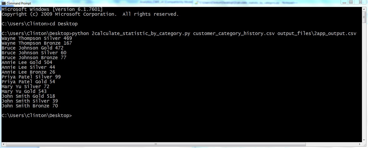
The output shown in the Command Prompt window reflects the output that was also written to 2app_output.csv. The contents of the file should look Figure 5-10. It shows the number of days each customer has had a specific package.
As you can see, the script wrote the header row to the output file and then wrote a row for every unique pair of customer names and package categories it processed from the input file. For example, the first two data rows beneath the header row show that Wayne Thompson had the Bronze package for 167 days and the Silver package for 469 days. The last three rows show that John Smith had the Bronze package for 70 days, the Silver package for 39 days, and the Gold package for 518 days. The remaining data rows show the results for the other customers. Having processed and aggregated the raw data in the input file, you can now calculate additional statistics with this data, summarize and visualize the data in different ways, or combine the data with other data for further analyses.
One note to point out is the business decision (a.k.a. assumption) we made about how to deal with the last package category for each customer. Presumably, if our input data is accurate and up to date, then the customer still has the last package category we have on record for the customer. For example, the last package category for Wayne Thompson is Silver, purchased on 6/29/2014. Because Wayne Thompson presumably still has this package, the amount of time assigned to this package should be the amount of time between today’s date and 6/29/2014, which means the amount of time added to the final package category for each customer depends on when you run the script.
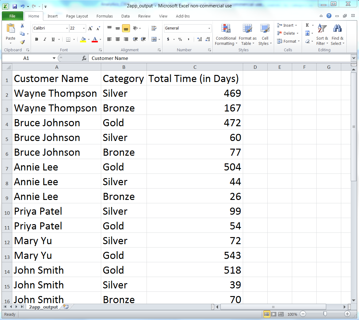
The code that implements this calculation and addition appears indented beneath line 34. Line 34 ensures that we do not try to calculate a difference for the first row of data, as we can’t calculate a difference based on one date. After processing the first row, line 35 sets first_row equal to False. Now, for all of the remaining data rows, line 35 is False, line 36 is not executed. For each transition from one customer to the next, lines 38 to 42 are executed. Line 38 calculates the difference (in days) between today’s date and the value in previous_package_date and assigns the integer value to the variable diff. Then, if the value in previous_package is not already a key in the inner dictionary, line 40 makes the value in previous_package a key in the inner dictionary and sets the associated value to the integer in diff. Alternatively, if the value in previous_package is already a key in the inner dictionary, then line 42 adds the integer in diff to the existing integer value associated with the corresponding key in the inner dictionary.
Returning to the Wayne Thompson example, the last package category for Wayne Thompson is Silver, with a purchse date of 6/29/2014. The next row of input data is for a different customer, Bruce Johnson, so the code beneath line 34 is executed. Running the script at the time I was writing this chapter, on 10/11/2015, resulted in the value in diff being 10/11/2015 minus 6/29/2014, or 469 days. As you can see in the Command Prompt window and in the output file shown previously, the amount of time recorded for Wayne Thompson and the Silver category is 469 days.
If you run this script on a different day, then the amount of time in this row of output, and all of the rows of output corresponding to each customer’s last package category, will be different (i.e., they should be larger numbers). How to deal with the last row of data for each customer is a business decision. You can always modify the code in this example to reflect how you want to treat the row for your specific use case.
This application combined several of the techniques we learned in Chapter 1, such as creating a user-defined function and populating a dictionary, to tackle a common, real-world problem. Business analysts often run into the problem of needing to calculate differences between values in rows of input data. In many cases, there are thousands or millions of rows that need to be handled in different ways, and the thought of having to calculate differences for particular rows manually is daunting (if the task is even possible).
In this section, we demonstrated a scalable way to calculate differences between values in rows and aggregate the differences based on values in other columns in the input file. To keep the setup to a minimum, the example only included a short list of customer records. However, the method scales well, so you can use it to perform calculations for a longer list of records or modify the code to process data from multiple input files.
Now that we’ve tackled the problem of calculating a statistic for an unknown number of categories, let’s turn to the problem of parsing a plain-text file for key pieces of data. This problem may sound a bit abstract right now, but let’s turn to the next section to learn more about this problem and how to tackle it.
The previous two applications demonstrated how to accomplish specific tasks with data in CSV and Excel files. Indeed, the majority of this book has focused on parsing and manipulating data in these files. For CSV files, we’ve used Python’s built-in csv module. For Excel files, we downloaded and have used the xlrd add-in module. CSV and Excel files are common file types in business, so it is important to understand how to deal with them.
At the same time, text files (a.k.a. flat files) are also a common file type in business. In fact, we already discussed how CSV files are actually stored as comma-delimited text files. A few more common examples of business data stored in text files are activity logs, error logs, and transaction records. Because text files, like CSV and Excel files, are common in business, and up to this point we haven’t focused on parsing text files, we’ll use this application to demonstrate how to extract data from text files and calculate statistics based on the data.
As mentioned in the previous paragraph, error logs are often stored in text files. The MySQL database system is one system that stores its error log as a text file. We downloaded and used the MySQL database system in the previous chapter, so if you followed along with the examples in the chapter, then you can access your MySQL system’s error log file. Keep in mind, however, that locating and viewing your MySQL system’s error log file is for your own edification; you do not have to access it to follow along with the example in this section.
To access your MySQL system’s error log file on Windows, open File Explorer, open the C: drive, open ProgramData, open the MySQL folder, open the MySQL Server <Version> folder (e.g., MySQL Server 5.6), and finally open the data folder. Inside the data folder, there should be an error log file that ends with the file extension .err. Right-click the file and open it with a text editor like Notepad or Notepad++ to view the errors your MySQL system has already written to the log file. If you cannot find one of the folders in this path, open File Explorer, open the C: drive, type “.err” in the search box in the upper-right corner, and wait for your system to find the error file. If your system finds many error files, then select the one with a path that is most similar to the one described above.
MacOS users should be able to find this file at /usr/local/mysql/data/<hostname>.err.
Because the data in your MySQL error log file is undoubtedly different from the data in my MySQL error log file, we’ll use a separate, representative MySQL error log file in this application. That way we can focus on the Python code instead of the idiosyncrasies of our different error log files. To create a typical MySQL error log file for this application, open a text editor, write the lines of text shown in Figure 5-11, and save the file as mysql_server_error_log.txt.
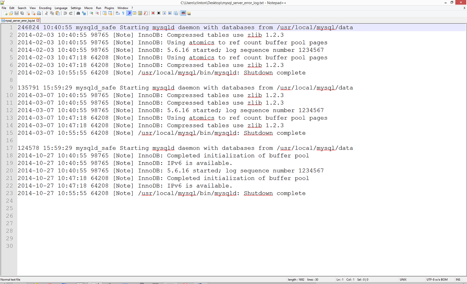
As you can see, a MySQL error log file contains information on when mysqld was started and stopped and also any critical errors that occurred while the server was running. For example, the first line in the file shows when mysqld was started and the seventh line shows when mysqld was stopped on that day. Lines 2–6 show the critical errors that occurred while the server was running on that day. These lines begin with a date and timestamp, and the critical error message is preceded by the term [Note]. The remaining lines in the file contain similar information for different days.
To reduce the amount of writing you need to do to create the file, I’ve repeated the timestamps and many of the critical error messages. Therefore, to create the file you really only need to write lines 1–7, copy and paste those lines twice, and then modify the dates and error messages.
Now that we have our MySQL error log text file, we need to discuss the business application. Text files like the one in this application often store disaggregated data, which can be parsed, aggregated, and analyzed for potential insights. For example, in this application, the error log file has recorded the types of errors that have occurred and when they have occurred. In its native layout, it is difficult to discern whether specific errors occur more frequently than other errors and whether the frequency of particular errors is changing over time. By parsing the text file, aggregating relevant pieces of data, and writing the output in a useful format, we can gain insights from the data that can drive corrective actions. The text files that you use may not be MySQL error logs, but being able to parse text files for key pieces of data and aggregate the data to generate insights is a skill that is generally applicable across text files.
Now that we understand the business application, all we need to do is write some Python code to carry out our error message binning and calculation tasks. To do so, type the following code into a text editor and save the file as 3parse_text_file.py:
1#!/usr/bin/env python32importsys3 4input_file=sys.argv[1]5output_file=sys.argv[2]6messages={}7notes=[]8withopen(input_file,'r',newline='')astext_file:9forrowintext_file:10if'[Note]'inrow:11row_list=row.split(' ',4)12day=row_list[0].strip()13note=row_list[4].strip('\n').strip()14ifnotenotinnotes:15notes.append(note)16ifdaynotinmessages:17messages[day]={}18ifnotenotinmessages[day]:19messages[day][note]=120else:21messages[day][note]+=122filewriter=open(output_file,'w',newline='')23header=['Date']24header.extend(notes)25header=','.join(map(str,header))+'\n'26(header)27filewriter.write(header)28forday,day_valueinmessages.items():29row_of_output=[]30row_of_output.append(day)31forindexinrange(len(notes)):32ifnotes[index]inday_value.keys():33row_of_output.append(day_value[notes[index]])34else:35row_of_output.append(0)36output=','.join(map(str,row_of_output))+'\n'37(output)38filewriter.write(output)39filewriter.close()
Because we are parsing a text file containing plain text in this application, instead of a CSV or Excel file, we do not need to import the csv or xlrd modules. We only need to import Python’s built-in string and sys modules, which we import in lines 2 and 3. As described previously, these two modules enable us to manipulate strings and read input from the command line, respectively.
Lines 4 and 5 take the two pieces of input we supply on the command line—the path to and name of the input text file that contains our MySQL error log data, and the path to and name of the CSV output file that will contain rows of information on the types of errors that occurred on different days—and assign the inputs to two separate variables (input_file and output_file, respectively).
Line 6 creates an empty dictionary called messages. Like the dictionary in the previous application, the messages dictionary will be a nested dictionary. The keys in the outer dictionary will be the specific days on which errors occurred. The value associated with each of these keys will be another dictionary. The keys in the inner dictionary will be unique error messages. The value associated with each one of these keys will be the number of times the error message occurred on the given day.
Line 7 creates an empty list called notes. The notes list will contain all of the unique error messages encountered across all of the days in the input error log file. Collecting all of the error messages in a separate data structure (i.e., in a list in addition to the dictionary) makes it easier to inspect all of the error messages found in the input error log file, write all of the error messages as the header row in the output file, and iterate through the dictionary and list separately to write the dates and counts data to the output file.
Line 8 uses Python’s with syntax to open the input text file for reading. Line 9 creates a for loop for looping over all of the rows in the input file.
Line 10 is an if statement that tests whether the string [Note] is in the row. The rows that contain the string [Note] are the rows that contain the error messages. You’ll notice that there is no else statement associated with the if statement, so the code doesn’t take any action for rows that do not contain the string [Note]. For rows that do contain the string [Note], lines 11 to 21 parse the rows and load specific pieces of data into our list and dictionary.
Line 11 uses the string module’s split() method to split the row on single spaces—up to four of them—and assigns the five split parts of the row into a list variable called row_list. We limit the number of times the split() method can split on single spaces because the first four space characters separate different pieces of data, whereas the remaining spaces appear in the error messages and should be retained as part of the error messages.
Line 12 takes the first element in row_list (a date) strips off any extra spaces, tabs, and newline characters from both ends of the date, and assigns the value to the variable day.
Line 13 takes the fifth element in row_list (the error message) strips off any extra spaces, tabs, and newline characters from both ends of the error message, and assigns the value to the variable, note.
Line 14 is an if statement that tests whether the error message contained in the variable note is not already contained in the list notes. If it is not, then line 15 uses the append() method to append the error message into the list. By testing whether it is already present and only adding an error message if it isn’t already in the list, we ensure we end up with a list of the unique error messages found in the input file.
Line 16 is an if statement that tests whether the date contained in the variable day is not already a key in the messages dictionary. If it is not, then line 17 adds the date as a key in the messages dictionary and creates an empty dictionary as the value associated with the new date key.
Line 18 is an if statement that tests whether the error message contained in the variable note is not already a key in the inner dictionary associated with a specific day. If it is not, then line 19 adds the error message as a key in the inner dictionary and sets the value associated with the key, a count, to the integer 1.
Line 20 is the else statement that complements the if statement in line 18. This line captures situations in which a particular error message appears more than once on a specific day. When this happens, line 21 increments the integer value associated with the error message by one. Lines 20 and 21 ensure that the final integer value associated with each error message reflects the number of times the error message appeared on a given day.
Once the script has finished processing all of the rows in the input error log file, the messages dictionary will be filled with key-value pairs. The keys will be all of the unique days on which error messages appeared. The values associated with these keys will be dictionaries with their own key-value pairs. The keys in these inner dictionaries will be the unique error messages that appeared on each of the recorded days, and the values associated with these keys will be integer counts of the number of times each error message appeared on each of the recorded days.
Line 22 opens the output file for writing and creates a writer object, filewriter, for writing to the output file.
Line 23 creates a list variable called header and assigns the string Date into the list. Line 24 uses the extend() method to extend the list variable header with the contents of the list variable notes. At this point, header contains the string Date as its first element and each of the unique error messages from notes as its remaining elements.
Line 25 uses the str() and map() functions and the join() method to transform the contents of the list variable header into one long string before it is written to the output file. The map() function applies the str() function to each of the values in header ensuring that each of the values in the variable is a string. Then the string module’s join() method inserts a comma between each of the string values in the variable header to create a long string of values separated by commas. Finally, a newline character is added to the end of the long string. This long string of column header values separated by commas with a newline character at the end is what will be written as the first row of output in the CSV output file.
Line 26 prints the value in header, the long string of column header values separated by commas, to the Command Prompt (or Terminal) window so you can inspect the output that will be written to the output file. Then line 27 uses the filewriter object’s write method to write the header row to the output file.
Line 28 creates a for loop that uses the items function to iterate over the keys (i.e., day) and values (i.e., day_value) in the messages dictionary. As we’ve done in previous examples, line 29 creates an empty list variable, row_of_output, that will hold each row of data that is written to the output file. Because we already wrote the header row to the output file, we know that the first column contains dates; therefore, we should expect that the first value appended into row_of_output is a date. Indeed, line 30 uses the append method to add the first date in the messages dictionary into row_of_output.
Next, lines 31–35 iterate through the error messages in the list variable notes and assess whether each error message occurred on the specific date being processed. If so, then the code adds the count associated with the error message in the correct position in the row. If the error message did not occur on the date being processed, then the code adds a zero in the correct position in the row.
Specifically, line 31 is a for loop that uses the range and len functions to iterate through the values in notes according to index position.
Line 32 is an if statement that tests whether each of the error messages in notes appears in the list of error messages associated with the date being processed. That is, day_value is the inner dictionary associated with the date being processed, and the keys function creates a list of the inner dictionary’s keys, which are the error messages associated with the date being processed.
For each error message in notes, if the error message appeared on the date being processed and, therefore, appears in the list of error messages associated with the date being processed, then line 33 uses the append method to append the count associated with the error message into row_of_output. By using the index values of the error messages in notes, you ensure that you retrieve the correct count for each error message.
For example, the first error message in the list notes is InnoDB: Compressed tables use zlib 1.2.3 so you can reference this string with notes[0]. As you’ll see in the Command Prompt/Terminal window when you run this script, this string is the header for the second column in the output file. You’ll also see in the screen output that this error message appeared three times on 2014-03-07.
Let’s review lines 28–35 in the script with this date and error message in mind to see how the correct data is written to the output file. Line 28 creates a for loop to loop through all of the dates in the messages dictionary, so at some point it will process 2014-03-07. When line 28 begins processing 2014-03-07, it also makes available the inner dictionary of error messages and their associated counts (because these are the keys and values in day_value). While processing 2014-03-07, line 31 creates another for loop to loop through the index values of the values in the notes list. The first time through the loop the index value is 0, so in line 32, notes[0] equals InnoDB: Compressed tables use zlib 1.2.3. Because we’re processing 2014-03-07, the value in notes[0] is in the set of keys in the inner dictionary associated with 2014-03-07. So, line 32 is True and line 33 is executed. In line 33, notes[index] becomes notes[0], day_value[notes[0]] becomes day_value["InnoDB: Compressed tables use zlib 1.2.3"], and that expression points to the value associated with that key in the inner dictionary, which for 2014-03-07 is the integer 3. The result of all of these operations is that that the number 3 appears in the output file in the row associated with 2014-03-07 and in the column associated with the error message InnoDB: Compressed tables use zlib 1.2.3.
Lines 34 and 35 handle the cases where the error messages in the list notes do not appear in the list of error messages recorded on a particular date. In these cases, line 35 adds a zero in the correct column for the row of output. For example, the last error message in the list notes is InnoDB: IPv6 is available. This error message did not appear on 2014-03-07, so the row of output for 2014-03-07 needs to record a zero in the column associated with this error message. When line 32 tests whether the last value in notes (notes[5], InnoDB: IPv6 is available.), is in the set of keys in the inner dictionary the result is False, so the else statement in line 34 is executed and line 35 appends a zero into row_of_output in the last column. The counts for the remaining dates and error messages are populated in a similar fashion.
Line 36 uses procedures identical to the ones in line 25 to transform the contents of the list variable row_of_output into one long string before it is written to the output file. The map function applies the str function to each of the values in the list variable row_of_output ensuring that each of the values in the variable is a string. Then the string module’s join method inserts a comma between each of the string values in the variable row_of_output to create a long string of values separated by commas. Finally, a newline character is added to the end of the long string. This long string of row values separated by commas with a newline character at the end is assigned to the variable output, which will be written as a row of output to the CSV output file.
Line 37 prints the value in output—the long string of row values separated by commas—to the Command Prompt or Terminal window so you can inspect the output that will be written to the output file. Then line 38 uses the filewriter object’s write method to write the row of output to the output file.
Finally, line 39 uses the filewriter’s close method to close the filewriter object.
Now that we have our Python script, let’s use our script to calculate the number of times different errors have occurred over time and write the output to a CSV-formatted output file. To do so, type the following on the command line, and then hit Enter:
python 3parse_text_file.py mysql_server_error_log.txt\ output_files\3app_output.csv
You should see the output shown in Figure 5-12 printed to your Command Prompt or Terminal window.
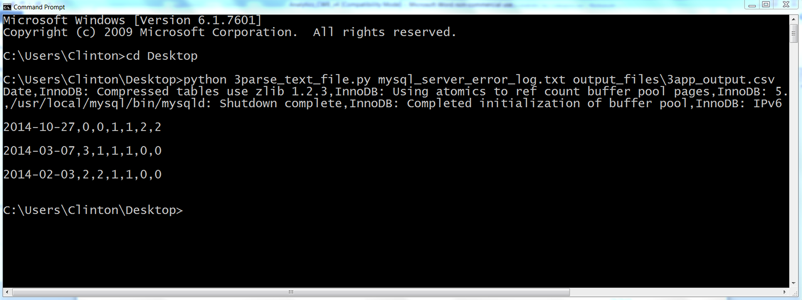
The output printed to the Command Prompt window shows the data that has also been written to the output file, 3app.output.csv. The first row of output is the header row, which shows the column headings for all of the columns in the output file. The first column heading, Date, shows that the first column contains the unique dates with error messages recorded in the input file. This column shows that the input file contained three unique dates. The remaining six column headings are the unique error messages that appeared in the input file; therefore, the input file contained six unique error messages. These six columns contain the counts of the number of times each particular error message appeared on each of the dates in the input file. For example, the final column of output shows that the error message InnoDB: IPv6 is available. appeared twice on 2014-10-27, zero times on 2014-02-03, and zero times on 2014-03-07.
The contents of 3app_output.csv, which reflect the output printed to the Command Prompt window, should look as shown in Figure 5-13.
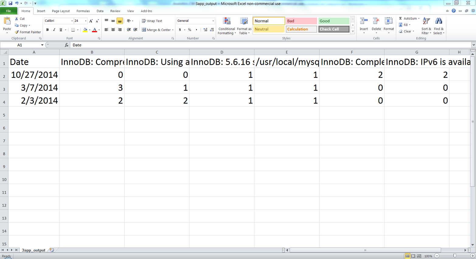
This screenshot of the CSV output file opened in Excel shows the data written in the output file. The six error messages appear in the header row after the Date heading, although you can’t see the complete messages in this screenshot because of horizontal space constraints (if you create this file, you can expand the columns to read the complete messages).
You will notice that the rows are for specific dates and the columns are for specific error messages. In this small example, there are more unique error messages (i.e., columns) than there are unique dates (i.e., rows). However, in larger log files, there are likely to be more unique dates than unique error messages. In that case, it makes sense to use the (more numerous) rows for specific dates and the columns for specific error messages. Ultimately, whether dates are in rows and error messages are in columns or vice versa depends on your analysis and preferences. A useful exercise for learning would be to modify the existing code to transpose the output, making the dates the columns and the error messages the rows.
This application combined several of the techniques we learned in Chapter 1, like populating a nested dictionary, to tackle a common, real-world problem. Business analysts often run into the problem of needing to parse text files for key pieces of data and aggregate or summarize the data for insights. In many cases, there are thousands or millions of rows that may need to be parsed in different ways, so it would be impossible to parse the rows manually.
In this section, we demonstrated a scalable way to parse data from rows in a text file and calculate basic statistics based on the parsed data. To keep the setup to a minimum, the example only used one short error log file. However, the method scales well, so you can use it to parse larger log files or modify the code to process data from multiple input text files.
The first application searches through input files that are saved in one specific folder. However, sometimes input files are saved in several nested folders. Modify the code in the first application so the script will traverse a set of nested folders and process the input files saved in all of the folders. Hint: search for “python os walk” on the Internet.2
Modify the second application to calculate the amount of revenue you have earned from customers in the Bronze, Silver, and Gold packages, if the Bronze package is $20/month, the Silver package is $40/month, and the Gold package is $50/month.
Practice using dictionaries to bin or group data into unique categories. For example, parse data from an Excel worksheet or a CSV file into a dictionary such that each column in the input file is a key-value pair in the dictionary. That is, each column heading is a key in the dictionary, and the list of values associated with each key are the data values in the associated column.
1 How much your computer can handle is based in large part on its random access memory (RAM) and central processing unit (CPU). Python stores data for processing in RAM, so when the size of your data is larger than your computer’s RAM, then your computer has to write data to disk instead of RAM. Writing to disk is much slower than storing data in RAM, so your computer will slow way down and seem to become unresponsive. If you think you might run into this problem based on the size of your data, you can use a machine that has more RAM, install more RAM in your machine, or process the data in smaller chunks. You can also use a distributed system, with lots of computers yoked together and acting as one, but that’s beyond the scope of this book.
2 You can learn about walking a directory tree at https://docs.python.org/3/library/os.html and http://www.pythoncentral.io/how-to-traverse-a-directory-tree-in-python-guide-to-os-walk/.
Creating figures and plots is an important step in many analytics projects, usually part of the exploratory data analysis (EDA) phase at the beginning of a project or the reporting phase, where you make your data analysis useful to others. Data visualization enables you to see your variables’ distributions, to see the relationships between your variables, and to check your modeling assumptions.
There are several plotting packages for Python, including matplotlib, pandas, ggplot, and seaborn. Because matplotlib is the most established package—and provides some of the underlying plotting concepts and syntax for the pandas and seaborn packages—we’ll cover it first. Then we’ll see some examples of how the other packages either simplify the plotting syntax or provide additional functionality.
matplotlib is a plotting package designed to create publication-quality figures. It has functions for creating common statistical graphs, including bar plots, box plots, line plots, scatter plots, and histograms. It also has add-in toolkits such as basemap and cartopy for mapping and mplot3d for 3D plotting.
matplotlib provides functions for customizing each component of a figure. For example, it enables you to specify the shape and size of the figure, the limits and scales of the x- and y-axes, the tick marks and labels of the x- and y-axes, the legend, and the title for the figure. You can learn more about customizing figures by perusing the matplotlib beginner’s guide and API.
The following examples demonstrate how to create some of the most common statistical graphs with matplotlib.
Bar plots represent numerical values, such as counts, for a set of categories. Common bar plots include vertical and horizontal plots, stacked plots, and grouped plots. The following script, bar_plot.py, illustrates how to create a vertical bar plot:
1#!/usr/bin/env python32importmatplotlib.pyplotasplt3plt.style.use('ggplot')4customers=['ABC','DEF','GHI','JKL','MNO']5customers_index=range(len(customers))6sale_amounts=[127,90,201,111,232]7fig=plt.figure()8ax1=fig.add_subplot(1,1,1)9ax1.bar(customers_index,sale_amounts,align='center',color='darkblue')10ax1.xaxis.set_ticks_position('bottom')11ax1.yaxis.set_ticks_position('left')12plt.xticks(customers_index,customers,rotation=0,fontsize='small')13plt.xlabel('Customer Name')14plt.ylabel('Sale Amount')15plt.title('Sale Amount per Customer')16plt.savefig('bar_plot.png',dpi=400,bbox_inches='tight')17plt.show()
Line 2 shows the customary import statement. Line 3 uses the ggplot stylesheet to emulate the aesthetics of ggplot2, a popular plotting package for R.
Lines 4, 5, and 6 create the data for the bar plot. I create a list of index values for the customers because the xticks function needs both the index locations and the labels to set the labels.
To create a plot in matplotlib, first you create a figure and then you create one or more subplots within the figure. Line 7 in this script creates a figure. Line 8 adds a subplot to the figure. Because it’s possible to add more than one subplot to a figure, you have to specify how many row and columns of subplots to create and which subplot to use. 1,1,1 indicates one row, one column, and the first and only subplot.
Line 9 creates the bar plot. customers_index specifies the x coordinates of the left sides of the bars. sale_amounts specifies the heights of the bars. align='center' specifies that the bars should be centered over their labels. color='darkblue' specifies the color of the bars.
Lines 10 and 11 remove the tick marks from the top and right of the plot by specifying that the tick marks should be on the bottom and left.
Line 12 changes the bars’ tick mark labels from the customers’ index numbers to their actual names. rotation=0 specifies that the tick labels should be horizontal instead of angled. fontsize='small' reduces the size of the tick labels.
Lines 13, 14, and 15 add the x-axis label, y-axis label, and title to the plot.
Line 16 saves the plot as bar_plot.png in the current folder. dpi=400 specifies the dots per inch for the saved plot, and bbox_inches='tight' trims empty whitespace around the saved plot.
Line 17 instructs matplotlib to display the plot in a new window on your screen. The result should look like Figure 6-1.
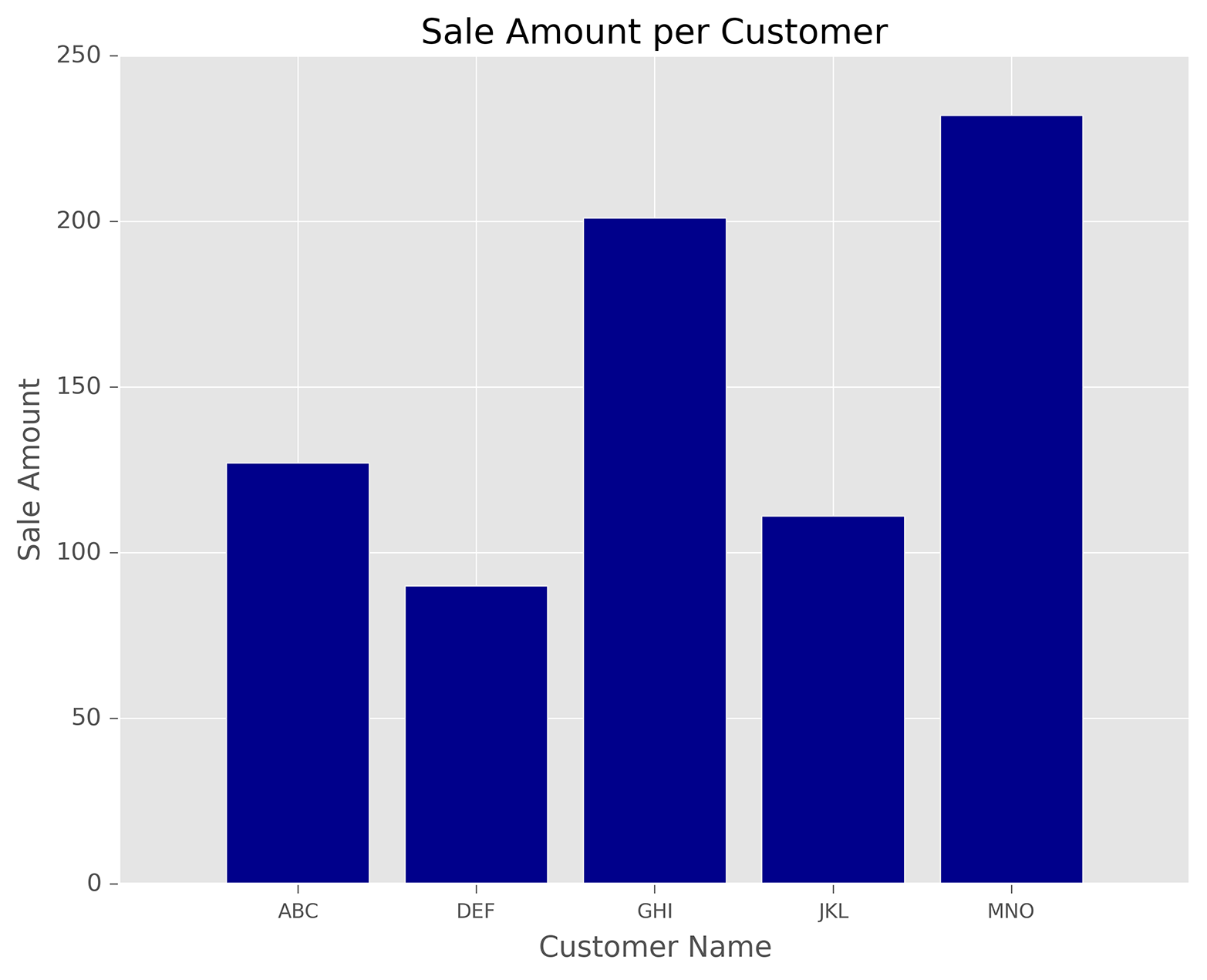
Histograms represent distributions of numerical values. Common histograms include frequency distributions, frequency density distributions, probability distributions, and probability density distributions. The following script, histogram.py, illustrates how to create a frequency distribution:
1#!/usr/bin/env python32importnumpyasnp3importmatplotlib.pyplotasplt4plt.style.use('ggplot')5mu1,mu2,sigma=100,130,156x1=mu1+sigma*np.random.randn(10000)7x2=mu2+sigma*np.random.randn(10000)8fig=plt.figure()9ax1=fig.add_subplot(1,1,1)10n,bins,patches=ax1.hist(x1,bins=50,normed=False,color='darkgreen')11n,bins,patches=ax1.hist(x2,bins=50,normed=False,color='orange',alpha=0.5)12ax1.xaxis.set_ticks_position('bottom')13ax1.yaxis.set_ticks_position('left')14plt.xlabel('Bins')15plt.ylabel('Number of Values in Bin')16fig.suptitle('Histograms',fontsize=14,fontweight='bold')17ax1.set_title('Two Frequency Distributions')18plt.savefig('histogram.png',dpi=400,bbox_inches='tight')19plt.show()
Lines 6 and 7 here use Python’s random-number generator to create two normally distributed variables, x1 and x2. The mean of x1 is 100 and the mean of x2 is 130, so the distributions will overlap but won’t lie on top of one another. Lines 10 and 11 create two histograms, or frequency distributions, for the variables. bins=50 means the values should be binned into 50 bins. normed=False means the histogram should display a frequency distribution instead of a probability density. The first histogram is dark green, and the second one is orange. alpha=0.5 means the second histogram should be more transparent so we can see the dark green bars where the two histograms overlap.
Line 16 adds a centered title to the figure, sets the font size to 14, and bolds the font. Line 17 adds a centered title to the subplot, beneath the figure’s title. We use these two lines to create a title and subtitle for the plot. Figure 6-2.
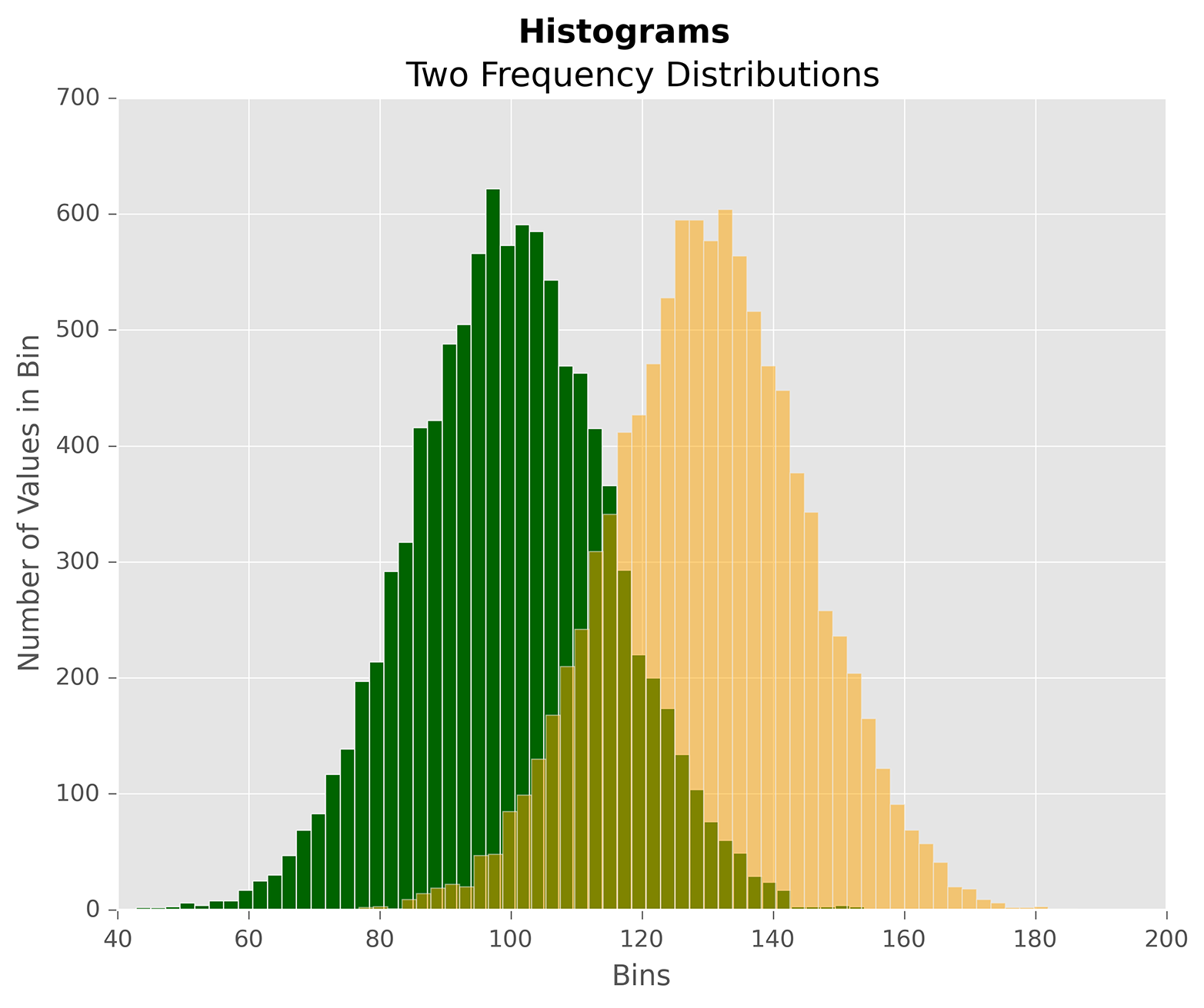
Line plots represent numerical values along a number line. It’s common to use line plots to show data over time. The following script, line_plot.py, illustrates how to create a line plot:
1#!/usr/bin/env python32fromnumpy.randomimportrandn3importmatplotlib.pyplotasplt4plt.style.use('ggplot')5plot_data1=randn(50).cumsum()6plot_data2=randn(50).cumsum()7plot_data3=randn(50).cumsum()8plot_data4=randn(50).cumsum()9fig=plt.figure()10ax1=fig.add_subplot(1,1,1)11ax1.plot(plot_data1,marker=r'o',color=u'blue',linestyle='-',\ 12label='Blue Solid')13ax1.plot(plot_data2,marker=r'+',color=u'red',linestyle='--',\ 14label='Red Dashed')15ax1.plot(plot_data3,marker=r'*',color=u'green',linestyle='-.',\ 16label='Green Dash Dot')17ax1.plot(plot_data4,marker=r's',color=u'orange',linestyle=':',\ 18label='Orange Dotted')19ax1.xaxis.set_ticks_position('bottom')20ax1.yaxis.set_ticks_position('left')21ax1.set_title('Line Plots: Markers, Colors, and Linestyles')22plt.xlabel('Draw')23plt.ylabel('Random Number')24plt.legend(loc='best')25plt.savefig('line_plot.png',dpi=400,bbox_inches='tight')26plt.show()
Again, we’re using randn to create (random) data to plot in lines 5–8. Lines 11–18 create four line plots. The lines use different types of data point markers, line colors, and line styles to illustrate some of the options. The label arguments ensure the lines are properly labeled in the legend.
Line 24 creates a legend for the plot. loc='best' instructs matplotlib to place the legend in the best location based on the open space in the plot. Alternatively, you can use this argument to specify a specific location for the legend. Figure 6-3 shows the line plots created by this script.
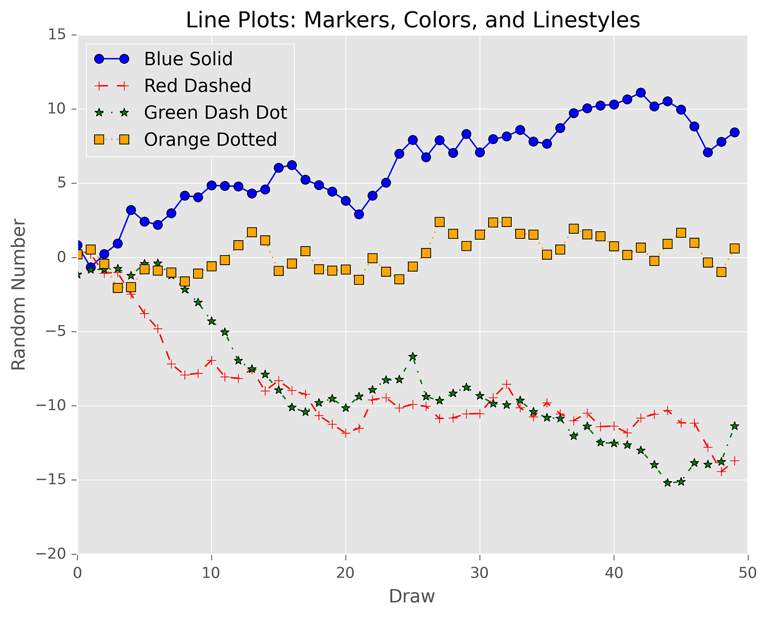
Scatter plots represent the values of two numerical variables along two axes—for example, height versus weight or supply versus demand. Scatter plots provide some indication of whether the variables are positively correlated (i.e., the points are concentrated in a specific configuration) or negatively correlated (i.e., the points are spread out like a diffuse cloud). You can also draw a regression line, the line that minimizes the squared error, through the points to make predictions for one variable based on values of the other variable.
The following script, scatter_plot.py, illustrates how to create a scatter plot with a regression line through the points:
1#!/usr/bin/env python32importnumpyasnp3importmatplotlib.pyplotasplt4plt.style.use('ggplot')5x=np.arange(start=1.,stop=15.,step=1.)6y_linear=x+5.*np.random.randn(14.)7y_quadratic=x**2+10.*np.random.randn(14.)8fn_linear=np.poly1d(np.polyfit(x,y_linear,deg=1))9fn_quadratic=np.poly1d(np.polyfit(x,y_quadratic,deg=2))10fig=plt.figure()11ax1=fig.add_subplot(1,1,1)12ax1.plot(x,y_linear,'bo',x,y_quadratic,'go',\13x,fn_linear(x),'b-',x,fn_quadratic(x),'g-',linewidth=2.)14ax1.xaxis.set_ticks_position('bottom')15ax1.yaxis.set_ticks_position('left')16ax1.set_title('Scatter Plots Regression Lines')17plt.xlabel('x')18plt.ylabel('f(x)')19plt.xlim((min(x)-1.,max(x)+1.))20plt.ylim((min(y_quadratic)-10.,max(y_quadratic)+10.))21plt.savefig('scatter_plot.png',dpi=400,bbox_inches='tight')22plt.show()
We cheat a little bit here by creating data (in lines 6 and 7) that uses random numbers to deviate just a bit from a linear and a quadratic polynomial equation—and then, in lines 8 and 9, we use numpy’s polyfit and poly1d functions to create linear and quadratic polynomial equations for the line and curve through the two sets of points (x, y_linear) and (x, y_quadratic). On real-world data, you can use the polyfit function to calculate the coefficients of the polynomial of fit based on the specified degree. The poly1d function uses the coefficients to create the actual polynomial equation.
Line 12 creates the scatter plot with the two regression lines. 'bo' means the (x, y_linear) points are blue circles, and 'go' means the (x, y_quadratic) points are green circles. Similarly, 'b-' means the line through the (x, y_linear) points is a solid blue line, and 'g-' means the line through the (x, y_quadratic) points is a solid green line. You specify the width of lines with linewidth.
Play around with these display variables to see what makes a chart with the aesthetic you’re looking for!
Lines 19 and 20 set the limits of the x-axis and y-axis. The lines use the min and max functions to create the axis limits based on the actual data values. You can also use specific numbers—for example, xlim(0, 20) and ylim(0, 200). If you don’t specify axis limits, matplotlib sets the limits for you. Figure 6-4 shows the result of running this script.
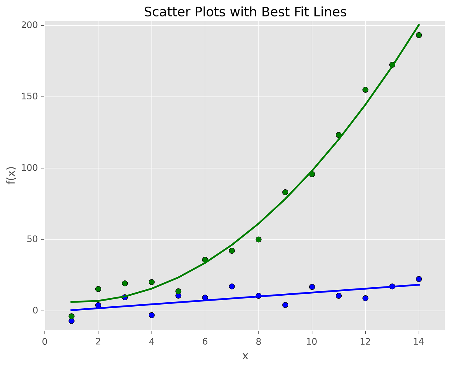
Box plots represent data based on its minimum, first quartile, median, third quartile, and maximum values. The bottom and top of the box show the first and third quartile values, and the line through the middle of the box shows the median value. The lines, called whiskers, that extend from the ends of the box show the smallest and largest non-outlier values, and the points beyond the whiskers represent outliers.
The following script, box_plot.py, illustrates how to create a box plot:
1#!/usr/bin/env python32importnumpyasnp3importmatplotlib.pyplotasplt4plt.style.use('ggplot')5N=5006normal=np.random.normal(loc=0.0,scale=1.0,size=N)7lognormal=np.random.lognormal(mean=0.0,sigma=1.0,size=N)8index_value=np.random.random_integers(low=0,high=N-1,size=N)9normal_sample=normal[index_value]10lognormal_sample=lognormal[index_value]11box_plot_data=[normal,normal_sample,lognormal,lognormal_sample]12fig=plt.figure()13ax1=fig.add_subplot(1,1,1)14box_labels=['normal','normal_sample','lognormal','lognormal_sample']15ax1.boxplot(box_plot_data,notch=False,sym='.',vert=True,whis=1.5,\16showmeans=True,labels=box_labels)17ax1.xaxis.set_ticks_position('bottom')18ax1.yaxis.set_ticks_position('left')19ax1.set_title('Box Plots: Resampling of Two Distributions')20ax1.set_xlabel('Distribution')21ax1.set_ylabel('Value')22plt.savefig('box_plot.png',dpi=400,bbox_inches='tight')23plt.show()
Line 14 creates a list named box_labels that contains labels for each of the box plots. We use this list in the boxplot function in the next line.
Line 15 uses the boxplot function to create the four box plots. notch=False means the boxes should be rectangular instead of notched in the middle. sym='.' means the flier points, the points beyond the whiskers, are dots instead of the default + symbol. vert=True means the boxes are vertical instead of horizontal. whis=1.5 specifies the reach of the whiskers beyond the first and third quartiles (e.g., Q3 + whis*IQR, IQR = interquartile range, Q3-Q1). showmeans=True specifies that the boxes should also show the mean value in addition to the median value. labels=box_labels means to use the values in box_labels to label the box plots.
Figure 6-5 shows the result of running this script.
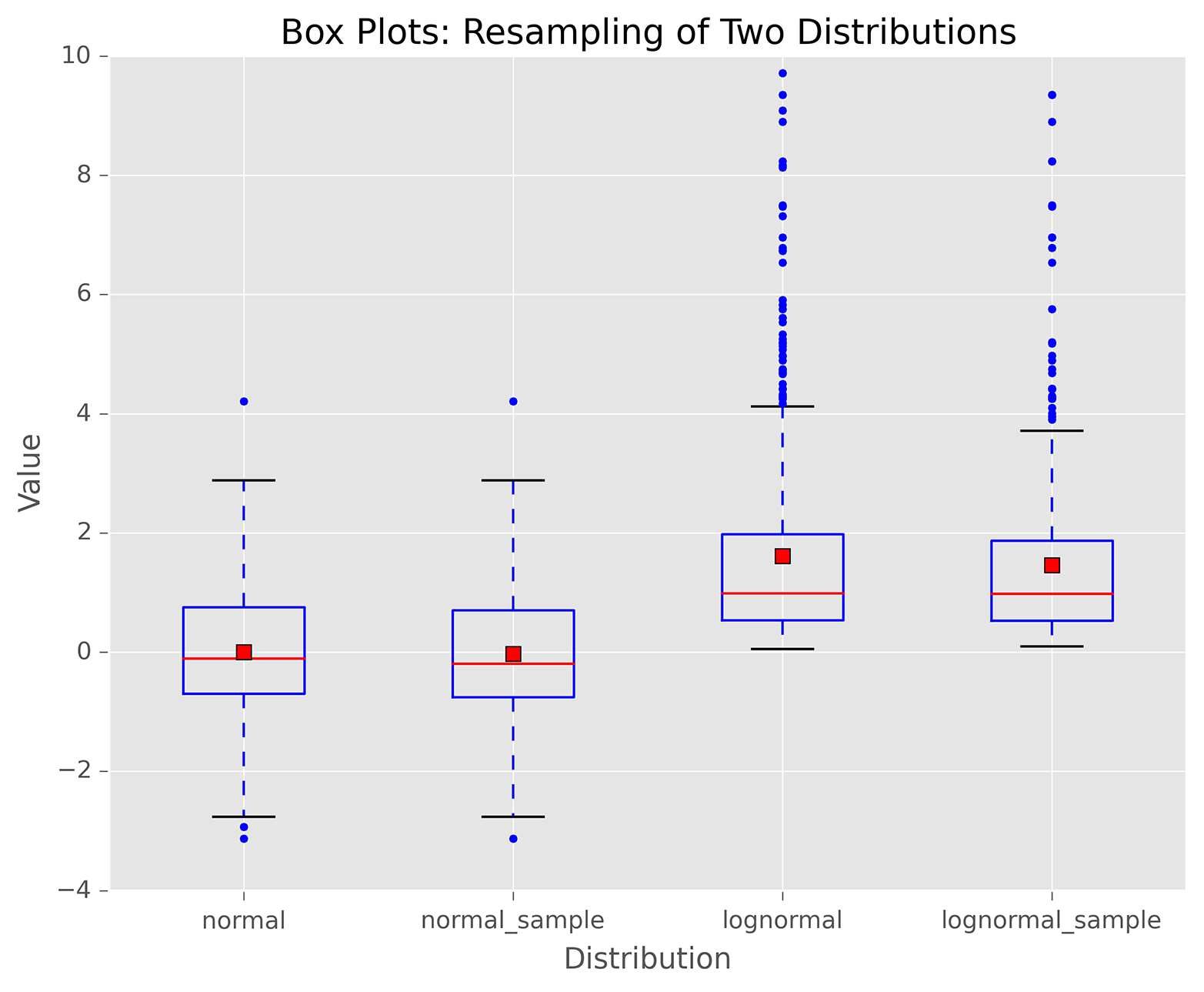
pandas simplifies the process of creating figures and plots based on data in Series and DataFrames by providing a plot function that operates on Series and DataFrames. By default, the plot function creates line plots, but you can use the kind argument to create different types of plots.
For example, in addition to the standard statistical plots you can create with matplotlib, pandas enables you to create other types of plots, such as hexagonal bin plots, scatter matrix plots, density plots, Andrews curves, parallel coordinates, lag plots, autocorrelation plots, and bootstrap plots. pandas also makes it straightforward to add a secondary y-axis, error bars, and a data table to a plot.
To illustrate how to create plots with pandas, the following script, pandas_plots.py, demonstrates how to create a pair of bar and box plots, side by side, based on data in a DataFrame:
1#!/usr/bin/env python32importpandasaspd3importnumpyasnp4importmatplotlib.pyplotasplt5plt.style.use('ggplot')6fig,axes=plt.subplots(nrows=1,ncols=2)7ax1,ax2=axes.ravel()8data_frame=pd.DataFrame(np.random.rand(5,3),9index=['Customer 1','Customer 2','Customer 3','Customer 4','Customer 5'],10columns=pd.Index(['Metric 1','Metric 2','Metric 3'],name='Metrics'))11data_frame.plot(kind='bar',ax=ax1,alpha=0.75,title='Bar Plot')12plt.setp(ax1.get_xticklabels(),rotation=45,fontsize=10)13plt.setp(ax1.get_yticklabels(),rotation=0,fontsize=10)14ax1.set_xlabel('Customer')15ax1.set_ylabel('Value')16ax1.xaxis.set_ticks_position('bottom')17ax1.yaxis.set_ticks_position('left')18colors=dict(boxes='DarkBlue',whiskers='Gray',medians='Red',caps='Black')19data_frame.plot(kind='box',color=colors,sym='r.',ax=ax2,title='Box Plot')20plt.setp(ax2.get_xticklabels(),rotation=45,fontsize=10)21plt.setp(ax2.get_yticklabels(),rotation=0,fontsize=10)22ax2.set_xlabel('Metric')23ax2.set_ylabel('Value')24ax2.xaxis.set_ticks_position('bottom')25ax2.yaxis.set_ticks_position('left')26plt.savefig('pandas_plots.png',dpi=400,bbox_inches='tight')27plt.show()
Line 6 creates a figure and a pair of side-by-side subplots. Line 7 uses the ravel function to separate the subplots into two variables, ax1 and ax2, so we don’t have to refer to the subplots with row and column indexing (e.g., axes[0,0] and axes[0,1]).
Line 12 uses the pandas plot function to create a bar plot in the lefthand subplot. Lines 13 and 14 use matplotlib functions to rotate and specify the size of the x- and y-axis labels.
Line 18 creates a dictionary of colors for individual box plot components. Line 19 creates the box plot in the righthand subplot, uses the colors variable to color the box plot components, and changes the symbol for outlier points to red dots.
Figure 6-6 shows the bar and box plots generated by this script. You can learn more about the types of plots you can create and how to customize them by perusing the pandas plotting documentation.
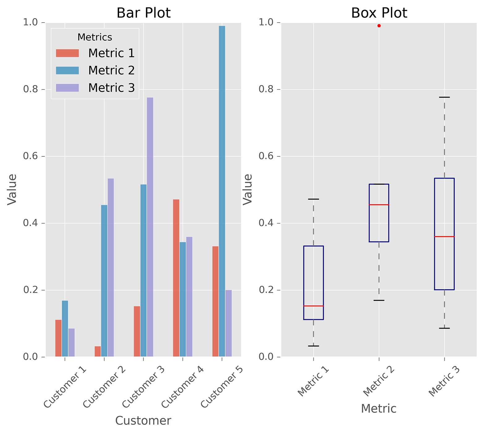
ggplot is a plotting package for Python based on R’s ggplot2 package and the Grammar of Graphics. One of the key differences between ggplot and other plotting packages is that its grammar makes a clear distinction between the data and what is actually displayed on the screen. To enable you to create a visual representation of your data, ggplot provides a few basic elements: geometries, aesthetics, and scales. It also provides some additional elements for more advanced plots: statistical transformations, coordinate systems, facets, and visual themes. Read Hadley Wickham’s ggplot2: Elegant Graphics for Data Analysis, Second Edition (Springer), for details on ggplot; you can also check out Grammar of Graphics, Second Edition (Springer), by Leland Wilkinson.
The ggplot package for Python isn’t as mature as R’s ggplot2 package, so it doesn’t have all of ggplot2’s features—that is, it doesn’t have as many geometries, statistics, or scales, and it doesn’t have any of the coordinate system, annotation, or fortify features (yet). You can also run into issues when developers upgrade and change packages that interact with ggplot. For example, I ran into an issue when I tried to create a histogram with ggplot because the pandas pivot_table’s rows and cols keywords were removed in favor of index and columns. Searching online for a solution, I discovered I had to change the word “rows” to the word “index” in a line in the file ggplot/stats/stat_bin.py to work around the issue.
Because ggplot has shortcomings relative to the other Python plotting packages I discuss in this chapter, I recommend you use one of the other packages to create your plots. However, I wanted to include this section on ggplot because I’m a fan of R’s ggplot2 package, and if you’re coming from R and you’re familiar with ggplot2, then you’ll immediately be able to use ggplot to create your graphs as long as it has the features you need.
The following script, ggplot_plots.py, demonstrates how to create a few basic plots with ggplot using datasets included in the ggplot package:
#!/usr/bin/env python3fromggplotimport*(mtcars.head())plt1=ggplot(aes(x='mpg'),data=mtcars)+\geom_histogram(fill='darkblue',binwidth=2)+\xlim(10,35)+ylim(0,10)+\xlab("MPG")+ylab("Frequency")+\ggtitle("Histogram of MPG")+\theme_matplotlib()(plt1)(meat.head())plt2=ggplot(aes(x='date',y='beef'),data=meat)+\geom_line(color='purple',size=1.5,alpha=0.75)+\stat_smooth(colour='blue',size=2.0,span=0.15)+\xlab("Year")+ylab("Head of Cattle Slaughtered")+\ggtitle("Beef Consumption Over Time")+\theme_seaborn()(plt2)(diamonds.head())plt3=ggplot(diamonds,aes(x='carat',y='price',colour='cut'))+\geom_point(alpha=0.5)+\scale_color_gradient(low='#05D9F6',high='#5011D1')+\xlim(0,6)+ylim(0,20000)+\xlab("Carat")+ylab("Price")+\ggtitle("Diamond Price by Carat and Cut")+\theme_gray()(plt3)ggsave(plt3,"ggplot_plots.png")
The three plots rely on the mtcars, meat, and diamonds datasets, which are included in ggplot. I print the head (first few lines) of each dataset to the screen before creating a plot to see the names of the variables and the initial data values.
The ggplot function takes as arguments the name of the dataset and the aesthetics, which specify how to use specific variables in the plot. The ggplot function is like matplotlib’s figure function in that it collects information to prepare for a plot but doesn’t actually display graphical elements like dots, bars, or lines. The next element in each plotting command, a geom, adds a graphical representation of the data to the plot. The three geoms add a histogram, line, and dots, respectively, to the plots. The remaining plotting functions add a title, axis limits and labels, and an overall layout and color theme to each plot.
Figure 6-7 shows the scatter plot this script creates. You can learn more about the types of plots you can create and how to customize them by perusing ggplot’s documentation.
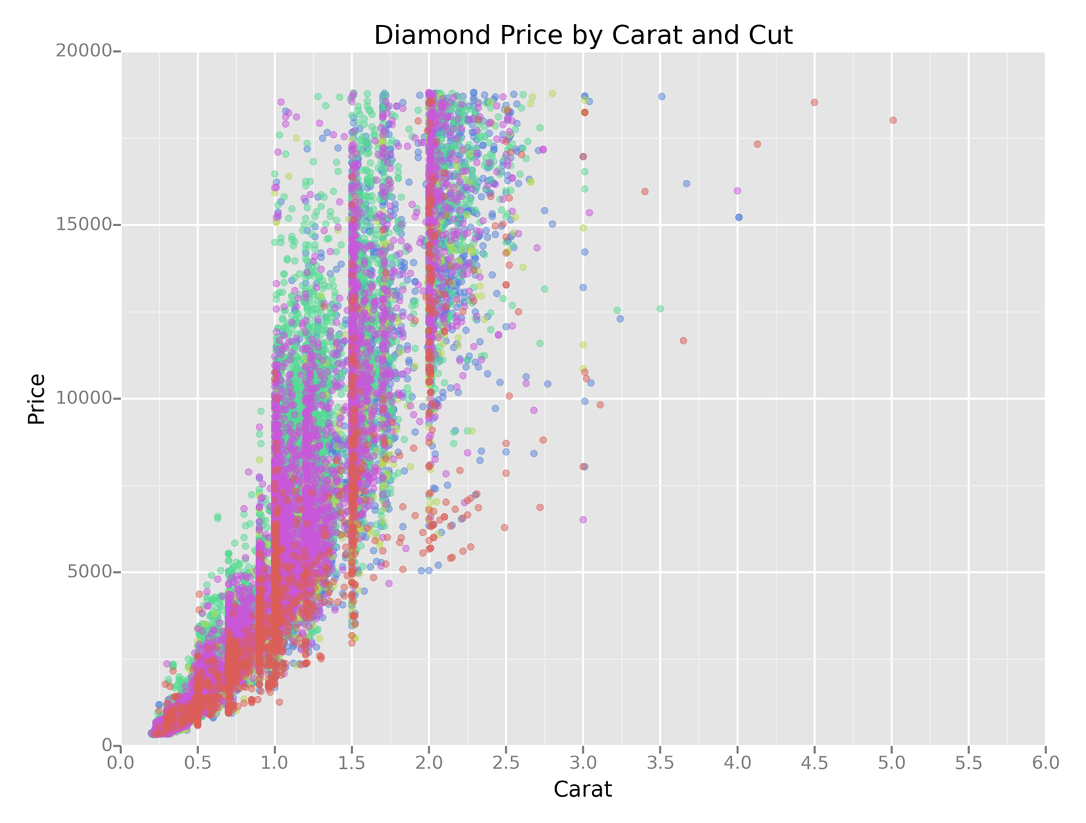
seaborn simplifies the process of creating informative statistical graphs and plots in Python. It is built on top of matplotlib, supports numpy and pandas data structures, and incorporates scipy and statsmodels statistical routines.
seaborn provides functions for creating standard statistical plots, including histograms, density plots, bar plots, box plots, and scatter plots. It has functions for visualizing pairwise bivariate relationships, linear and nonlinear regression models, and uncertainty around estimates. It enables you to inspect a relationship between variables while conditioning on other variables, and to build grids of plots to display complex relationships. It has built-in themes and color palettes you can use to make beautiful graphs. Finally, because it’s built on matplotlib, you can further customize your plots with matplotlib commands.
The following script, seaborn_plots.py, demonstrates how to create a variety of statistical plots with seaborn:
#!/usr/bin/env python3importseabornassnsimportnumpyasnpimportpandasaspdimportmatplotlib.pyplotaspltfrompylabimportsavefigsns.set(color_codes=True)# Histogramx=np.random.normal(size=100)sns.distplot(x,bins=20,kde=False,rug=True,label="Histogram w/o Density")sns.axlabel("Value","Frequency")plt.title("Histogram of a Random Sample from a Normal Distribution")plt.legend()# Scatter plot with regression line and univariate graphsmean,cov=[5,10],[(1,.5),(.5,1)]data=np.random.multivariate_normal(mean,cov,200)data_frame=pd.DataFrame(data,columns=["x","y"])sns.jointplot(x="x",y="y",data=data_frame,kind="reg")\.set_axis_labels("x","y")plt.suptitle("Joint Plot of Two Variables with Bivariate and Univariate Graphs")# Pairwise bivariate scatter plots with univariate histogramsiris=sns.load_dataset("iris")sns.pairplot(iris)# Box plots conditioning on several variablestips=sns.load_dataset("tips")sns.factorplot(x="time",y="total_bill",hue="smoker",\col="day",data=tips,kind="box",size=4,aspect=.5)# Linear regression model with bootstrap confidence intervalsns.lmplot(x="total_bill",y="tip",data=tips)# Logistic regression model with bootstrap confidence intervaltips["big_tip"]=(tips.tip/tips.total_bill)>.15sns.lmplot(x="total_bill",y="big_tip",data=tips,logistic=True,y_jitter=.03)\.set_axis_labels("Total Bill","Big Tip")plt.title("Logistic Regression of Big Tip vs. Total Bill")plt.show()savefig("seaborn_plots.png")
The first plot, shown in Figure 6-8, uses the distplot function to display a histogram. The example shows how you can specify the number of bins, display or not display the Gaussian kernel density estimate (kde), display a rugplot on the support axis, create axis labels and a title, and create a label for a legend.
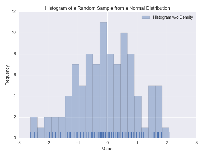
The second plot, shown in Figure 6-9, uses the jointplot function to display a scatter plot of two variables with a regression line through the points and histograms for each of the variables.
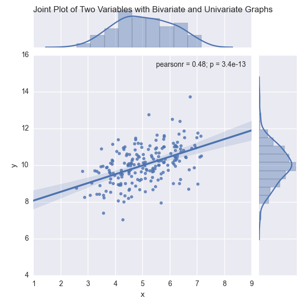
The third plot, shown in Figure 6-10, uses the pairplot function to display pairwise bivariate scatter plots and histograms for all of the variables in the dataset.
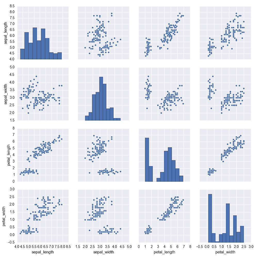
The fourth plot, shown in Figure 6-11, uses the factorplot function to display box plots of the relationship between two variables for different values of a third variable, while conditioning on another variable.
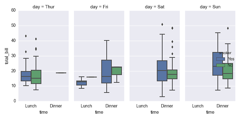
The fifth plot, shown in Figure 6-12, uses the lmplot function to display a scatter plot and linear regression model through the points. It also displays a bootstrap confidence interval around the line.
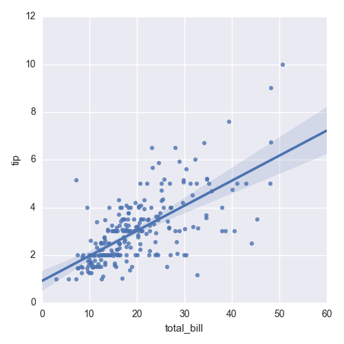
The sixth plot, shown in Figure 6-13, uses the lmplot function to display a logistic regression model for a binary dependent variable. The function uses the y_jitter argument to slightly jitter the ones and zeros so it’s easier to see where the points cluster along the x-axis.
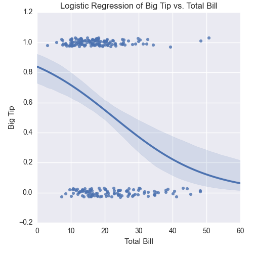
These examples are meant to give you an idea of the types of plots you can create with seaborn, but they only scratch the surface of seaborn’s functionality. You can learn more about the types of plots you can create and how to customize them by perusing seaborn’s documentation.
The earlier chapters in this book focused on a variety of data processing techniques that enable you to transform raw data into a dataset that’s ready for statistical analysis. In this chapter, we turn our attention to some of these basic statistical analysis and modeling techniques. We’ll focus on exploring and summarizing datasets with plots and summary statistics and conducting regression and classification analyses with multivariate linear regression and logistic regression.
This chapter isn’t meant to be a comprehensive treatment of statistical analysis techniques or pandas functionality. Instead, the goal is to demonstrate how you can produce some standard descriptive statistics and models with pandas and statsmodels.
Instead of creating datasets with thousands of rows from scratch, let’s download them from the Internet. One of the datasets we’ll use is the Wine Quality dataset, which is available at the UC Irvine Machine Learning Repository. The other dataset is the Customer Churn dataset, which has been featured in several analytics blog posts.
The Wine Quality dataset consists of two files, one for red wines and one for white wines, for variants of the Portuguese “Vinho Verde” wine. The red wines file contains 1,599 observations and the white wines file contains 4,898 observations. Both files contain one output variable and eleven input variables. The output variable is quality, which is a score between 0 (low quality) and 10 (high quality). The input variables are physicochemical characteristics of the wine, including fixed acidity, volatile acidity, citric acid, residual sugar, chlorides, free sulfur dioxide, total sulfur dioxide, density, pH, sulphates, and alcohol.
The two datasets are available for download at the following URLs:
Rather than analyze these two datasets separately, let’s combine them into one dataset. After you combine the red and white files into one file, the resulting dataset should have one header row and 6,497 observations. It is also helpful to add a column that indicates whether the wine is red or white. The dataset we’ll use looks as shown in Figure 7-1 (note the row numbers on the lefthand side and the additional “type” variable in column A).
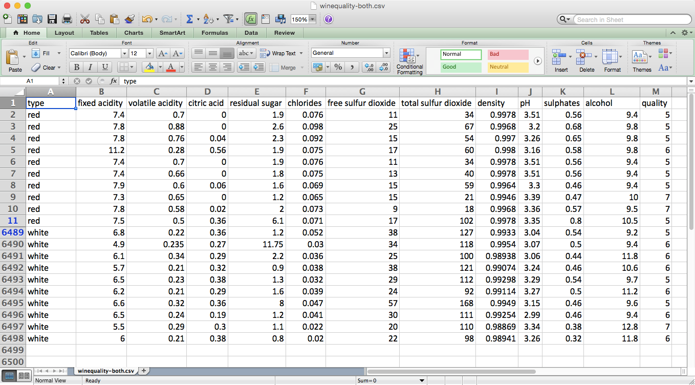
The Customer Churn dataset is one file that contains 3,333 observations of current and former telecommunications company customers. The file has one output variable and twenty input variables. The output variable, Churn?, is a Boolean (True/False) variable that indicates whether the customer had churned (i.e., was no longer a customer) by the time of the data collection.
The input variables are characteristics of the customer’s phone plan and calling behavior, including state, account length, area code, phone number, has an international plan, has a voice mail plan, number of voice mail messages, daytime minutes, number of daytime calls, daytime charges, evening minutes, number of evening calls, evening charges, nighttime minutes, number of nighttime calls, nighttime charges, international minutes, number of international calls, international charges, and number of customer service calls.
The dataset is available for download at Churn.
The dataset looks as shown in Figure 7-2.
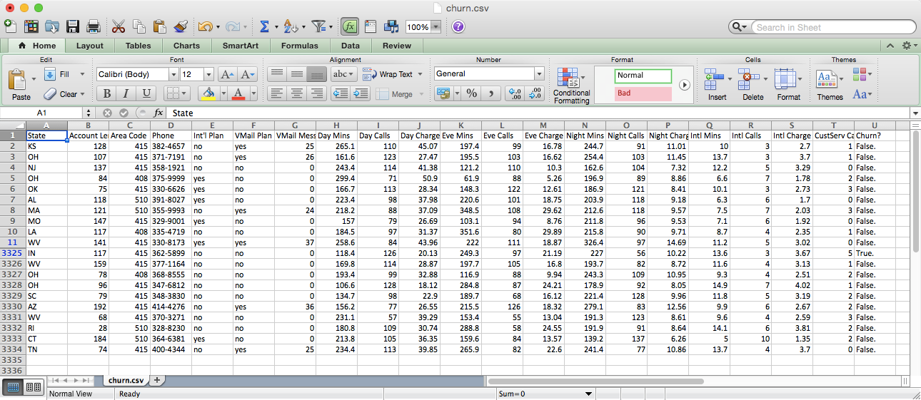
Let’s analyze the Wine Quality dataset first. To start, let’s display overall descriptive statistics for each column, the unique values in the quality column, and observation counts for each of the unique values in the quality column. To do so, create a new script, wine_quality.py, and add the following initial lines of code:
#!/usr/bin/env python3importnumpyasnpimportpandasaspdimportseabornassnsimportmatplotlib.pyplotaspltimportstatsmodels.apiassmimportstatsmodels.formula.apiassmffromstatsmodels.formula.apiimportols,glm# Read the dataset into a pandas DataFramewine=pd.read_csv('winequality-both.csv',sep=',',header=0)wine.columns=wine.columns.str.replace(' ','_')(wine.head())# Display descriptive statistics for all variables(wine.describe())# Identify unique values(sorted(wine.quality.unique()))# Calculate value frequencies(wine.quality.value_counts())
After the import statements, the first thing we do is use the pandas read_csv function to read the text file winequality-both.csv into a pandas DataFrame. The extra arguments indicate that the field separator is a comma and the column headings are in the first row. Some of the column headings contain spaces (e.g., “fixed acidity”), so in the next line we replace the spaces with underscores. Next, we use the head function to view the header row and the first five rows of data to check that the data is loaded correctly.
Line 14 uses the pandas describe function to print summary statistics for each of the numeric variables in the dataset. The statistics it reports are count, mean, standard deviation, minimum value, 25th percentile value, median value, 75th percentile value, and maximum value. For example, there are 6,497 observations of quality scores. The scores range from 3 to 9, and the mean quality score is 5.8 with a standard deviation of 0.87.
The following line identifies the unique values in the quality column and prints them to the screen in ascending order. The output shows that the unique values in the quality column are 3, 4, 5, 6, 7, 8, and 9.
Finally, the last line in this section counts the number of times each unique value in the quality column appears in the dataset and prints them to the screen in descending order. The output shows that 2,836 observations have a quality score of 6; 2,138 observations have a score of 5; 1,079 observations have a score of 7; 216 observations have a score of 4; 193 observations have a score of 8; 30 observations have a score of 3; and 5 observations have a score of 9.
The preceding statistics are for the entire dataset, which combines both the red and white wines. Let’s see if the statistics remain similar when we evaluate the red and white wines separately:
# Display descriptive statistics for quality by wine type(wine.groupby('type')[['quality']].describe().unstack('type'))# Display specific quantile values for quality by wine type(wine.groupby('type')[['quality']].quantile([0.25,0.75]).unstack('type'))# Look at the distribution of quality by wine typered_wine=wine.loc[wine['type']=='red','quality']white_wine=wine.loc[wine['type']=='white','quality']sns.set_style("dark")(sns.distplot(red_wine,\norm_hist=True,kde=False,color="red",label="Red wine"))(sns.distplot(white_wine,\norm_hist=True,kde=False,color="white",label="White wine"))sns.axlabel("Quality Score","Density")plt.title("Distribution of Quality by Wine Type")plt.legend()plt.show()# Test whether mean quality is different between red and white wines(wine.groupby(['type'])[['quality']].agg(['std']))tstat,pvalue,df=sm.stats.ttest_ind(red_wine,white_wine)('tstat:%.3fpvalue:%.4f'%(tstat,pvalue))
The first line in this section prints the summary statistics for red and white wines separately. The groupby function uses the type column to separate the data into two groups based on the two values in this column. The square brackets enable us to list the set of columns for which we want to produce output. In this case, we only want to apply the describe function to the quality column. The result of these commands is a single column of statistics where the results for red and white wines are stacked vertically on top of one another. The unstack function reformats the results so the statistics for the red and white wines are displayed horizontally in two separate columns.
The next line is very similar to the preceding line, but instead of using the describe function to display several descriptive statistics, it uses the quantile function to display the 25th and 75th percentile values from the quality column.
Next, we use seaborn to create a plot of two histograms, as shown in Figure 7-3: one for the red wines and one for the white wines.
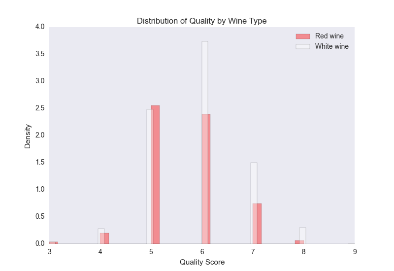
The red bars are for the red wines and the white bars are for the white wines. Because there are more white wines than red wines (4,898 white compared to 1,599 red), the plot displays normalized/density distributions instead of frequency distributions. The plot shows that quality scores for both red and white wines are approximately normally distributed. Compared to the raw summary statistics, the histograms make it easier to see the distributions of quality scores for the two types of wines.
Finally, we conduct a t-test to evaluate whether the mean quality scores for the red and white wines are different. This code illustrates how to use the groupby and agg functions to calculate a set of statistics for separate groups in a dataset. In this case, we want to know whether the standard deviations of the quality scores for the red and white wines are similar, in which case we can use pooled variance in the t-test. The t-statistic is –9.69 and the p-value is 0.00, which indicates that the mean quality score for white wines is statistically greater than the mean quality score for red wines.
Now that we’ve examined the output variable, let’s briefly explore the input variables. Let’s calculate the correlation between all pairs of variables and also create a few scatter plots with regression lines for a subset of the variables:
# Calculate correlation matrix for all variables(wine.corr())# Take a "small" sample of red and white wines for plottingdeftake_sample(data_frame,replace=False,n=200):returndata_frame.loc[np.random.choice(data_frame.index,\replace=replace,size=n)]reds_sample=take_sample(wine.loc[wine['type']=='red',:])whites_sample=take_sample(wine.loc[wine['type']=='white',:])wine_sample=pd.concat([reds_sample,whites_sample])wine['in_sample']=np.where(wine.index.isin(wine_sample.index),1.,0.)(pd.crosstab(wine.in_sample,wine.type,margins=True))# Look at relationship between pairs of variablessns.set_style("dark")g=sns.pairplot(wine_sample,kind='reg',plot_kws={"ci":False,\"x_jitter":0.25,"y_jitter":0.25},hue='type',diag_kind='hist',\diag_kws={"bins":10,"alpha":1.0},palette=dict(red="red",white="white"),\markers=["o","s"],vars=['quality','alcohol','residual_sugar'])(g)plt.suptitle('Histograms and Scatter Plots of Quality, Alcohol, and Residual\Sugar',fontsize=14,horizontalalignment='center',verticalalignment='top',\x=0.5,y=0.999)plt.show()
The corr function calculates the linear correlation between all pairs of variables in the dataset. Based on the sign of the coefficients, the output suggests that alcohol, sulphates, pH, free sulfur dioxide, and citric acid are positively correlated with quality, whereas fixed acidity, volatile acidity, residual sugar, chlorides, total sulfur dioxide, and density are negatively correlated with quality.
There are over 6,000 points in the dataset, so it will be difficult to see distinct points if we plot all of them. To address this issue, the second section defines a function, take_sample, which we’ll use to create a small sample of points that we can use in plots. The function uses pandas DataFrame indexing and numpy’s random.choice function to select a random subset of rows. We use this function to take a sample of red wines and a sample of white wines, and then we concatenate these DataFrames into a single DataFrame. Then we create a new column in our wine DataFrame named in_sample and use numpy’s where function and the pandas isin function to fill the column with ones and zeros depending on whether the row’s index value is one of the index values in the sample. Finally, we use the pandas crosstab function to confirm that the in_sample column contains 400 ones (200 red wines and 200 white wines) and 6,097 zeros.
seaborn’s pairplot function creates a matrix of plots. The plots along the main diagonal display the univariate distributions for each of the variables either as densities or histograms. The plots on the off-diagonal display the bivariate distributions between each pair of variables as scatter plots either with or without regression lines.
The pairwise plot in Figure 7-4 shows the relationships between quality, alcohol, and residual sugar. The red bars and dots are for the red wines and the white bars and dots are for the white wines. Because the quality scores only take on integer values, I’ve slightly jittered them so it’s easier to see where they’re concentrated.
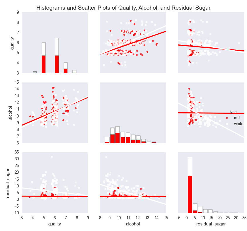
The plots show that the mean and standard deviation values of alcohol for red and white wines are similar, whereas the mean and standard deviation values of residual sugar for white wines are greater than the corresponding values for red wines. The regression lines suggest that quality increases as alcohol increases for both red and white wines, whereas quality decreases as residual sugar increases for both red and white wines. In both cases, the effect appears to be greater for white wines than for red wines.
Correlation coefficients and pairwise plots and are helpful for quantifying and visualizing the bivariate relationships between variables, but they don’t measure the relationships between the dependent variable and each independent variable while controlling for the other independent variables. Linear regression addresses this issue.
Linear regression refers to the following model:
yi ~ N(μi, σ2),
μi = β0 + β1xi1 + β2xi2 + ... + βpxip
for i = 1, 2, ..., n observations and p independent variables.
This model indicates that observation yi is drawn from a normal (Gaussian) distribution with a mean μi, which depends on the independent variables, and a constant variance σ2. That is, given an observation’s values for the independent variables, we observe a specific quality score. On another day with the same values for the independent variables, we might observe a different quality score. However, over many days with the same values for the independent variables (i.e., in the long run), the quality score would fall in the range defined by μi ± σ.
Now that we understand the linear regression model, let’s use the statsmodels package to run a linear regression:
my_formula='quality ~ alcohol + chlorides + citric_acid + density\+ fixed_acidity + free_sulfur_dioxide + pH + residual_sugar + sulphates\+ total_sulfur_dioxide + volatile_acidity'lm=ols(my_formula,data=wine).fit()## Alternatively, a linear regression using generalized linear model (glm) syntax## lm = glm(my_formula, data=wine, family=sm.families.Gaussian()).fit()(lm.summary())("\nQuantities you can extract from the result:\n%s"%dir(lm))("\nCoefficients:\n%s"%lm.params)("\nCoefficient Std Errors:\n%s"%lm.bse)("\nAdj. R-squared:\n%.2f"%lm.rsquared_adj)("\nF-statistic:%.1fP-value:%.2f"%(lm.fvalue,lm.f_pvalue))("\nNumber of obs:%dNumber of fitted values:%d"%(lm.nobs,\len(lm.fittedvalues)))
The first line assigns a string to a variable named my_formula. The string contains R-style syntax for specifying a regression formula. The variable to the left of the tilde (~), quality, is the dependent variable and the variables to the right of the tilde are the independent explanatory variables.
The second line fits an ordinary least-squares regression model using the formula and data and assigns the results to a variable named lm. To demonstrate a similar formulation, the next (commented-out) line fits the same model using the generalized linear model (glm) syntax instead of the ordinary least-squares syntax.
The next seven lines print specific model quantities to the screen. The first line prints a summary of the results to the screen. This summary is helpful because it displays the coefficients, their standard errors and confidence intervals, the adjusted R-squared, the F-statistic, and additional model details in one display.
The next line prints a list of all of the quantities you can extract from lm, the model object. Reviewing this list, I’m interested in extracting the coefficients, their standard errors, the adjusted R-squared, the F-statistic and its p-value, and the fitted values.
The next four lines extract these values. lm.params returns the coefficient values as a Series, so you can extract individual coefficients by position or name. For example, to extract the coefficient for alcohol, 0.267, you can use lm.params[1] or lm.params['alcohol']. Similarly, lm.bse returns the coefficients’ standard errors as a Series. lm.rsquared_adj returns the adjusted R-squared and lm.fvalue and lm.f_pvalue return the F-statistic and its p-value, respectively. Finally, lm.fittedvalues returns the fitted values. Rather than display all of the fitted values, I display the number of them next to the number of observations, lm.nobs, to confirm that they’re the same length. The output is shown in Figure 7-5.
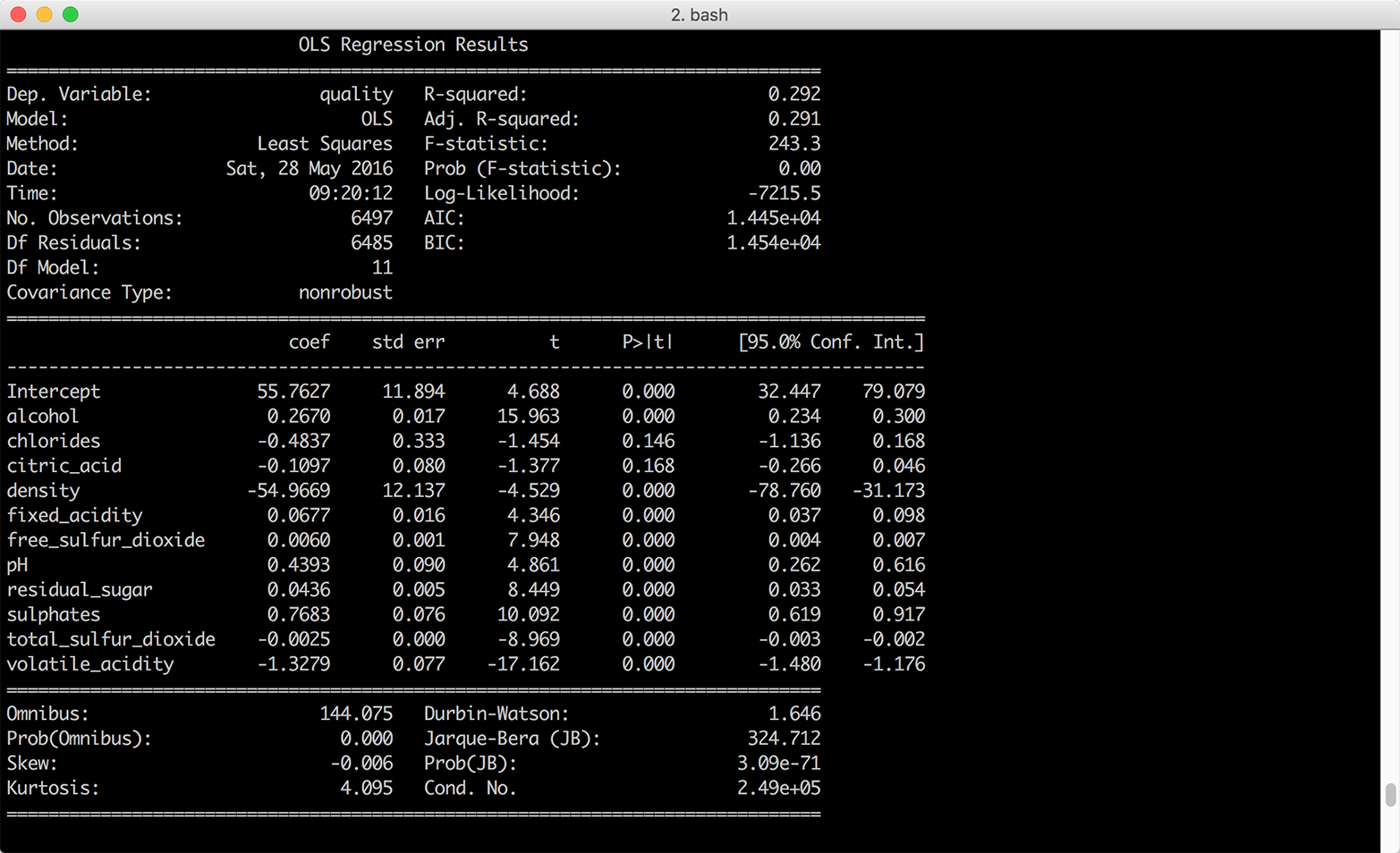
If you were going to use this model to understand the relationships between the dependent variable, wine quality, and the independent variables, the eleven wine characteristics, you would want to interpret the coefficients. Each coefficient represents the average difference in wine quality, comparing wines that differ by one unit on the specific independent variable and are otherwise identical. For example, the coefficient for alcohol suggests that, on average, comparing two wines that have the same values for all of the remaining independent variables, the quality score of the wine with one more unit of alcohol will be 0.27 points greater than that of the wine with less alcohol content.
It isn’t always worthwhile to interpret all of the coefficients. For example, the coefficient on the intercept represents the expected quality score when the values for all of the independent variables are set to zero. Because there aren’t any wines with zeros for all of their wine characteristics, the coefficient on the intercept isn’t meaningful.
Another aspect of the model to keep in mind is that ordinary least-squares regression estimates the values for the unknown β parameters by minimizing the sum of the squared residuals, the deviations of the dependent variable observations from the fitted function. Because the sizes of the residuals depend on the units of measurement of the independent variables, if the units of measurement vary greatly you can make it easier to interpret the model by standardizing the independent variables. You standardize a variable by subtracting the variable’s mean from each observation and dividing each result by the variable’s standard deviation. By standardizing a variable, you make its mean 0 and its standard deviation 1.1
Using wine.describe(), we can see that chlorides varies from 0.009 to 0.661 while total sulfur dioxide varies from 6.0 to 440.0. The remaining variables have similar differences between their minimum and maximum values. Given the disparity between the ranges of values for each of the independent variables, it’s worthwhile to standardize the independent variables to see if doing so makes it easier to interpret the results.
pandas makes it very easy to standardize variables in a DataFrame. You write the equation you would write for one observation, and pandas broadcasts it across all of the rows and columns to standardize all of the variables. The following lines of code create a new DataFrame, wine_standardized, with independent variables:
# Create a Series named dependent_variable to hold the quality datadependent_variable=wine['quality']# Create a DataFrame named independent variables to hold all of the variables# from the original wine dataset except quality, type, and in_sampleindependent_variables=wine[wine.columns.difference(['quality','type',\'in_sample'])]# Standardize the independent variables. For each variable,# subtract the variable's mean from each observation and# divide each result by the variable's standard deviationindependent_variables_standardized=(independent_variables-\independent_variables.mean())/independent_variables.std()# Add the dependent variable, quality, as a column in the DataFrame of# independent variables to create a new dataset with# standardized independent variableswine_standardized=pd.concat([dependent_variable,independent_variables\_standardized],axis=1)
Now that we have a dataset with standardized independent variables, let’s rerun the regression and view the summary (Figure 7-6):
lm_standardized = ols(my_formula, data=wine_standardized).fit() print(lm_standardized.summary())
Standardizing the independent variables changes how we interpret the coefficients. Now each coefficient represents the average standard deviation difference in wine quality, comparing wines that differ by one standard deviation on the specific independent variable and are otherwise identical. For example, the coefficient for alcohol suggests that, on average, comparing two wines that have the same values for all of the remaining independent variables, the quality score of the wine with one standard deviation more alcohol will be 0.32 standard deviations greater than that of the wine with less alcohol content.
Using wine.describe() again, we can see that the mean and standard deviation values for alcohol are 10.5 and 1.2 and the mean and standard deviation values for quality are 5.8 and 0.9. Therefore, comparing two wines that are otherwise identical, we would expect the quality score of the one that has alcohol content 11.7 (10.5 + 1.2) to be 0.32 standard deviations greater than that of the one with mean alcohol content, on average.
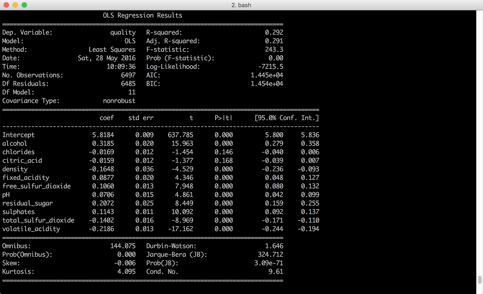
Standardizing the independent variables also changes how we interpret the intercept. With standardized explanatory variables, the intercept represents the mean of the dependent variable when all of the independent variables are at their mean values. In our model summary, the coefficient on the intercept suggests that when all of the wine characteristics are at their mean values we should expect the mean quality score to be 5.8 with a standard error of 0.009.
In some situations, you may be interested in making predictions for new data that wasn’t used to fit the model. For example, you may receive new observations of wine characteristics, and you want to predict the wine quality scores for the wines based on their characteristics. Let’s illustrate making predictions for new data by selecting the first 10 observations of our existing dataset and predicting their quality scores based on their wine characteristics.
To be clear, we’re using observations we used to fit the model for convenience and illustration purposes only. Outside of this example, you will want to evaluate your model on data you didn’t use to fit the model, and you’ll make predictions on new observations. With this caveat in mind, let’s create a set of “new” observations and predict the quality scores for these observations:
# Create 10 "new" observations from the first 10 observations in the wine dataset# The new observations should only contain the independent variables used in the# modelnew_observations=wine.ix[wine.index.isin(range(10)),\independent_variables.columns]# Predict quality scores based on the new observations' wine characteristicsy_predicted=lm.predict(new_observations)# Round the predicted values to two decimal placess and print them to the screeny_predicted_rounded=[round(score,2)forscoreiny_predicted](y_predicted_rounded)
The variable y_predicted contains the 10 predicted values. I round the predicted values to two decimal places simply to make the output easier to read. If the observations we used in this example were genuinely new, we could use the predicted values to evaluate the model. In any case, we have predicted values we can assess and use for other purposes.
Now let’s analyze the Customer Churn dataset. To start, let’s read the data into a DataFrame, reformat the column headings, create a numeric binary churn variable, and view the first few rows of data. To do so, create a new script, customer_churn.py, and add the following initial lines of code:
#!/usr/bin/env python3importnumpyasnpimportpandasaspdimportseabornassnsimportmatplotlib.pyplotaspltimportstatsmodels.apiassmimportstatsmodels.formula.apiassmfchurn=pd.read_csv('churn.csv',sep=',',header=0)churn.columns=[heading.lower()forheadingin\churn.columns.str.replace(' ','_').str.replace("\'","").str.strip('?')]churn['churn01']=np.where(churn['churn']=='True.',1.,0.)(churn.head())
After the import statements, the first line reads the data into a DataFrame named churn. The next line uses the replace function twice to replace spaces with underscores and delete embedded single quotes in the column headings. Note that the second replace function has a backslashed single quote between double quotes followed by a comma and then a pair of double quotes. This line uses the strip function to remove the question mark at the end of the Churn? column heading. Finally, the line uses a list comprehension to convert all of the column headings to lowercase.
The next line creates a new column named churn01 and uses numpy’s where function to fill it with ones and zeros based on the values in the churn column. The churn column contains the values True and False, so the churn01 column contains a one where the value in the churn column is True and a zero where the value is False.
The last line uses the head function to display the header row and the first five rows of data so we can check that the data is loaded correctly and the column headings are formatted correctly.
Now that we’ve loaded the data into a DataFrame, let’s see if we can find any differences between people who churned and people who didn’t churn by calculating descriptive statistics for the two groups. This code groups the data into two groups, those who churned and those who didn’t churn, based on the values in the churn column. Then it calculates three statistics—count, mean, and standard deviation—for each of the listed columns separately for the two groups:
# Calculate descriptive statistics for grouped data(churn.groupby(['churn'])[['day_charge','eve_charge','night_charge',\'intl_charge','account_length','custserv_calls']].agg(['count','mean',\'std']))
The following line illustrates how you can calculate different sets of statistics for different variables. It calculates the mean and standard deviation for four variables and the count, minimum, and maximum for two variables. We group by the churn column again, so it calculates the statistics separately for those who churned and those who didn’t churn:
# Specify different statistics for different variables(churn.groupby(['churn']).agg({'day_charge':['mean','std'],'eve_charge':['mean','std'],'night_charge':['mean','std'],'intl_charge':['mean','std'],'account_length':['count','min','max'],'custserv_calls':['count','min','max']}))
The next section of code summarizes the customer service calls data with five statistics—count, minimum, mean, maximum, and standard deviation—after grouping the data into five equal-width bins based on the values in a new total_charges variable. To do so, the first line creates a new variable, total_charges, which is the sum of the day, evening, night, and international charges. The next line uses the cut function to split total_charges into five equal-width groups. Then I define a function, get_stats, which will return a dictionary of statistics for each group. The next line groups the customer service calls data into the five total_charges groups. Finally, I apply the get_stats function to the grouped data to calculate the statistics for the five groups:
# Create total_charges, split it into 5 groups, and# calculate statistics for each of the groupschurn['total_charges']=churn['day_charge']+churn['eve_charge']+\churn['night_charge']+churn['intl_charge']factor_cut=pd.cut(churn.total_charges,5,precision=2)defget_stats(group):return{'min':group.min(),'max':group.max(),'count':group.count(),'mean':group.mean(),'std':group.std()}grouped=churn.custserv_calls.groupby(factor_cut)(grouped.apply(get_stats).unstack())
Like the previous section, this next section summarizes the customer service calls data with five statistics. However, this section uses the qcut function to split account_length into four equal-sized bins (i.e., quantiles), instead of equal-width bins:
# Split account_length into quantiles and# calculate statistics for each of the quantilesfactor_qcut=pd.qcut(churn.account_length,[0.,0.25,0.5,0.75,1.])grouped=churn.custserv_calls.groupby(factor_qcut)(grouped.apply(get_stats).unstack())
By splitting account_length into quantiles, we ensure that each group contains approximately the same number of observations. The equal-width bins in the previous section did not contain the same number of observations in each group. The qcut function takes an integer or an array of quantiles to specify the number of quantiles, so you can use the number 4 instead of [0., 0.25, 0.5, 0.75, 1.] to specify quartiles or 10 to specify deciles.
The following code illustrates how to use the pandas get_dummies function to create binary indicator variables and add them to a DataFrame. The first two lines create binary indicator variables for the intl_plan and vmail_plan columns and prefix the new columns with the original variable names. The next line uses the join command to merge the churn column with the new binary indicator columns and assigns the result into a new DataFrame named churn_with_dummies. The new DataFrame has five columns, churn, intl_plan_no, intl_plan_yes, vmail_plan_no, and vmail_plan_yes:
# Create binary/dummy indicator variables for intl_plan and vmail_plan# and join them with the churn column in a new DataFrameintl_dummies=pd.get_dummies(churn['intl_plan'],prefix='intl_plan')vmail_dummies=pd.get_dummies(churn['vmail_plan'],prefix='vmail_plan')churn_with_dummies=churn[['churn']].join([intl_dummies,vmail_dummies])(churn_with_dummies.head())
This code illustrates how to split a column into quartiles, create binary indicator variables for each of the quartiles, and add the new columns to the original DataFrame. The qcut function splits the total_charges column into quartiles and labels each quartile with the names listed in qcut_names. The get_dummies function creates four binary indicator variables for the quartiles and prefixes the new columns with total_charges. The result is four new dummy variables, total_charges_1st_quartile, total_charges_2nd_quartile, total_charges_3rd_quartile, and total_charges_4th_quartile. The join function appends these four variables into the churn DataFrame:
# Split total_charges into quartiles, create binary indicator variables# for each of the quartiles, and add them to the churn DataFrameqcut_names=['1st_quartile','2nd_quartile','3rd_quartile','4th_quartile']total_charges_quartiles=pd.qcut(churn.total_charges,4,labels=qcut_names)dummies=pd.get_dummies(total_charges_quartiles,prefix='total_charges')churn_with_dummies=churn.join(dummies)(churn_with_dummies.head())
The final section of code creates three pivot tables. The first line calculates the mean value for total_charges after pivoting, or grouping, on churn and the number of customer service calls. The result is a long column of numbers for each of the churn and number of customer service calls buckets. The second line specifies that the output should be reformatted so that churn defines the rows and number of customer service calls defines the columns. Finally, the third line uses the number of customer service calls for the rows, churn for the columns, and demonstrates how to specify the statistic you want to calculate, the value to use for missing values, and whether to display margin values:
# Create pivot tables(churn.pivot_table(['total_charges'],index=['churn','custserv_calls']))(churn.pivot_table(['total_charges'],index=['churn'],\columns=['custserv_calls']))(churn.pivot_table(['total_charges'],index=['custserv_calls'],\columns=['churn'],aggfunc='mean',fill_value='NaN',margins=True))
In this dataset, the dependent variable is binary. It indicates whether the customer churned and is no longer a customer. Linear regression isn’t appropriate in this case because it can produce predicted values that are less than 0 and greater than 1, which doesn’t make sense for probabilities. Because the dependent variable is binary, we need to constrain the predicted values to be between 0 and 1. Logistic regression produces this result.
Logistic regression refers to the following model:
Pr(yi = 1) = logit–1(β0 + β1xi1 + β2xi2 + ... + βpxip)
for i = 1, 2, ..., n observations and p input variables.
Equivalently:
Pr(yi = 1) = pi
logit(pi) = β0 + β1xi1 + β2xi2 + ... + βpxip
Logistic regression measures the relationships between the binary dependent variable and the independent variables by estimating probabilities using the inverse logit (or logistic) function. The function transforms continuous values into values between 0 and 1, which is imperative since the predicted values represent probabilities and probabilities must be between 0 and 1. In this way, logistic regression predicts the probability of a particular outcome, such as churning.
Logistic regression estimates the values for the unknown β parameters by applying an iterative algorithm that solves for the maximum likelihood estimates.
The syntax we need to use for a logistic regression is slightly different from the syntax for a linear regression. For a logistic regression we specify the dependent variable and independent variables separately instead of in a formula:
dependent_variable=churn['churn01']independent_variables=churn[['account_length','custserv_calls',\'total_charges']]independent_variables_with_constant=sm.add_constant(independent_variables,\prepend=True)logit_model=sm.Logit(dependent_variable,independent_variables_with_constant)\.fit()(logit_model.summary())("\nQuantities you can extract from the result:\n%s"%dir(logit_model))("\nCoefficients:\n%s"%logit_model.params)("\nCoefficient Std Errors:\n%s"%logit_model.bse)
The first line creates a variable named dependent_variable and assigns it the series of values in the churn01 column.
Similarly, the second line specifies the three columns we’ll use as the independent variables and assigns them to a variable named independent_variables.
Next, we add a column of ones to the input variables with statsmodels’s add_constant function.
The next line fits a logistic regression model and assigns the results to a variable named logit_model.
The last four lines print specific model quantities to the screen. The first line prints a summary of the results to the screen. This summary is helpful because it displays the coefficients, their standard errors and confidence intervals, the pseudo R-squared, and additional model details in one display.
The next line prints a list of all of the quantities you can extract from logit_model, the model object. Reviewing this list, I’m interested in extracting the coefficients and their standard errors.
The next two lines extract these values. logit_model.params returns the coefficient values as a Series, so you can extract individual coefficients by position or name. Similarly, logit_model.bse returns the coefficients’ standard errors as a Series. The output is shown in Figure 7-7.
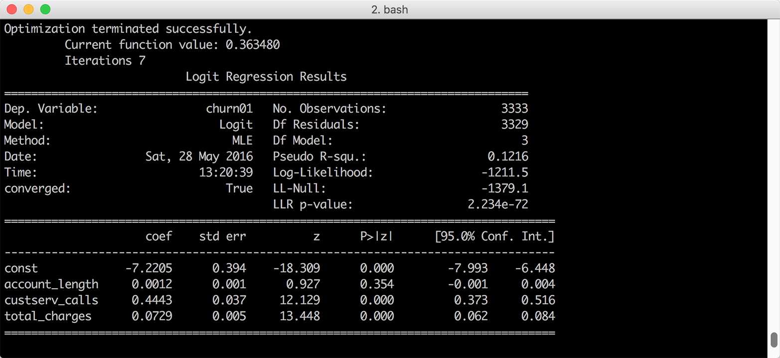
Interpreting the regression coefficients for a logistic regression isn’t as straightforward as it is for a linear regression because the inverse logistic function is curved, which means the expected difference in the dependent variable for a one-unit change in an independent variable isn’t constant.
Because the inverse logistic function is curved, we have to select where to evaluate the function to assess the impact on the probability of success. As with linear regression, the coefficient for the intercept represents the probability of success when all of the independent variables are zero. Sometimes zero values don’t make sense, so an alternative is to evaluate the function with all of the independent variables set to their mean values:
definverse_logit(model_value):frommathimportexpreturn(1.0/(1.0+exp(-model_value)))at_means=float(logit_model.params[0])+\float(logit_model.params[1])*float(churn['account_length'].mean())+\float(logit_model.params[2])*float(churn['custserv_calls'].mean())+\float(logit_model.params[3])*float(churn['total_charges'].mean())("Probability of churn at mean values:%.2f"%inverse_logit(at_means))
The first block of code defines a function named inverse_logit that transforms the continuous predicted values from the linear model into probabilities between 0 and 1.
The second block of code estimates the predicted value for an observation where all of the independent variables are set to their mean values. The four logit_model.params[...] values are the model coefficients and the three churn['...'].mean() values are the mean values of the account length, customer service calls, and total charges columns. Given the model coefficients and the mean values, this equation is approximately –7.2 + (0.001 * 101.1) + (0.444 * 1.6) + (0.073 * 59.5), so the value in the variable at_means is –2.068.
The last line of code prints the inverse logit of the value in at_means, formatted to two decimal places, to the screen. The inverse logit of –2.068 is 0.112, so the probability of a person churning whose account length, customer service calls, and total charges are equal to the average values for these variables is 11.2 percent.
Similarly, to evaluate the change in the dependent variable for a one-unit change in one of the dependent variables, we can evaluate the difference in the probability by changing one of the dependent variables by one unit close to its mean value.
For example, let’s evaluate the impact of a one-unit change in the number of customer service calls, close to this variable’s mean value, on the probability of churning:
cust_serv_mean=float(logit_model.params[0])+\float(logit_model.params[1])*float(churn['account_length'].mean())+\float(logit_model.params[2])*float(churn['custserv_calls'].mean())+\float(logit_model.params[3])*float(churn['total_charges'].mean())cust_serv_mean_minus_one=float(logit_model.params[0])+\float(logit_model.params[1])*float(churn['account_length'].mean())+\float(logit_model.params[2])*float(churn['custserv_calls'].mean()-1.0)+\float(logit_model.params[3])*float(churn['total_charges'].mean())("Probability of churn when account length changes by 1:%.2f"%\(inverse_logit(cust_serv_mean)-inverse_logit(cust_serv_mean_minus_one)))
The first block of code is identical to the code for at_means. The second block of code is nearly identical, except we’re subtracting one from the mean number of customer service calls.
Finally, in the last line of code we’re subtracting the inverse logit of the estimated value when two of the variables are at their mean values and the value for number of customer service calls is set to its mean value minus one from the inverse logit of the estimated value when all of the independent variables are set to their mean values.
In this case, the value in cust_serv_mean is the same as the value in at_means, –2.068. The value in cust_serv_means_minus_one is –2.512. The result of the inverse logit of –2.068 minus the inverse logit of –2.512 is 0.0372, so one additional customer service call near the mean number of calls corresponds to a 3.7 percent higher probability of churning.
As we did in the section “Making Predictions”, we can also use the fitted model to make predictions for “new” observations:
# Create 10 "new" observations from the first 10 observations# in the churn datasetnew_observations=churn.ix[churn.index.isin(range(10)),\independent_variables.columns]new_observations_with_constant=sm.add_constant(new_observations,prepend=True)# Predict probability of churn based on the new observations'# account characteristicsy_predicted=logit_model.predict(new_observations_with_constant)# Round the predicted values to two decimal places and print them to the screeny_predicted_rounded=[round(score,2)forscoreiny_predicted](y_predicted_rounded)
Again, the variable y_predicted contains the 10 predicted values and I’ve rounded the predicted values to two decimal places to make the output easier to read. Now we have predicted values we can use, and if the observations we used in this example were genuinely new we could use the predicted values to evaluate the model.
1 In Data Analysis Using Regression and Multilevel/Hierarchical Models (Cambridge University Press, 2007, p. 56), Gelman and Hill suggest dividing by two standard deviations instead of one standard deviation in situations where your dataset contains both binary and continuous independent variables so that a one-unit change in your standardized variables corresponds to a change from one standard deviation below to one standard deviation above the mean. Because the wine quality dataset doesn’t contain binary independent variables, I standardize the independent variables into z-scores by dividing by one standard deviation.
We’ve covered a lot of ground up to this point in the book. After reviewing Python basics, we processed text files, CSV files, Excel files, and data in databases, and applied our new knowledge to three common business analysis applications. In these examples, we’ve run the scripts manually on the command line. For example:
python my_python_script.py input_file.txt output_file.csv
This method of running scripts is common and completely acceptable, but what happens when you plan to run a script on a regular basis? Without another method of running the script, you have to be available and remember to run the script manually on the command line. As you can imagine, this method isn’t optimal for scripts that should be run on a regular basis. In this situation, we need another method to regularly schedule scripts to run.
Both Windows and macOS have programs for running scripts and other executable files on a regular basis. Microsoft calls its program Task Scheduler; the program that does this on Unix and macOS is called cron (you may have heard of crontab files or cron jobs). This book has focused on running scripts on Windows, so the next section will demonstrate how to schedule a Python script to run regularly on Windows with Task Scheduler. At the same time, it is useful to know how to schedule cron jobs on macOS or Unix, so we will also demonstrate how to use cron to schedule a Python script to run regularly on those operating systems.
To demonstrate how to schedule a Python script to run regularly on Windows with Task Scheduler, we need to choose a Python script. For simplicity, let’s use the script we created in the final application in Chapter 5, 3parse_text_file.py. In that application, we used the script to parse a MySQL error log file. The application actually works well in this case because an error log file is one type of file that usually needs to be analyzed on a regular basis. For example, you may analyze a database error log file on a daily, weekly, or monthly basis to understand the frequency of specific errors to focus maintenance and correction efforts. Finally, while this example demonstrates how to schedule a Python script to run regularly, remember that you can use Task Scheduler to schedule other types of scripts and executable files too.
To begin, ensure the two files we created in the last application in Chapter 5 (i.e., 3parse_text_file.py and mysql_server_error_log.txt) are saved on your Desktop. If you save the two files on your Desktop, then the file paths in the following instructions and screenshots will be easy to understand. Of course, you can save the files in different locations and change the file paths in Task Scheduler to point to where you’ve saved the files on your computer.
To open Task Scheduler, click the Start button, navigate to Control Panel→System and Security→Administrative Tools, and then double-click Task Scheduler (see Figure 8-1). If you’re prompted for an administrator password or confirmation, type the password or provide confirmation.
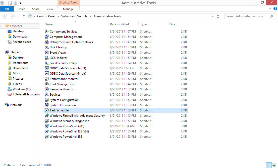
Note the file path at the top of the screen: Control Panel→System and Security→Administrative Tools. In the list of administrative tools, Task Scheduler is highlighted in a blue rectangle.
Task Scheduler will open after you double-click it. When Task Scheduler opens, you will see the screen shown in Figure 8-2.
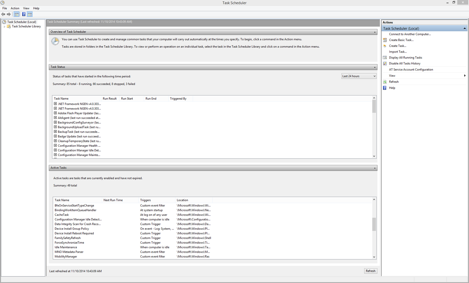
Notice the list of available actions in the upper-right corner (e.g., Connect to Another Computer, Create Basic Task, etc.). These actions are also available under the Action menu in the upper-left corner.
To schedule a task, click the Action menu in the upper-left corner, and then click Create Basic Task (alternatively, double-click Create Basic Task in the upper-right corner). In either case, the Create Basic Task Wizard opens.
Name and describe your task by filling in the Name and Description fields in the wizard home screen (see Figure 8-3). Because we’re creating a task to run a Python script to parse an error log file on a regular basis, we’ll name the task “Parse Error Log File” and give it this description: “This task schedules a Python script, 3parse_text_file.py, to parse an error log file on a monthly basis.” Once you’ve filled in the Name and Description fields, click Next.
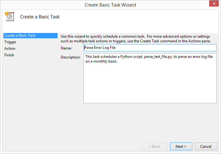
When you click Next, the task wizard will transition to the Trigger tab (see Figure 8-4). On the Trigger tab, you select when you want the task to start. Because we’ve decided we want our script to run on a monthly basis, let’s select the Monthly radio button. Once you’ve selected the Monthly radio button, click Next.
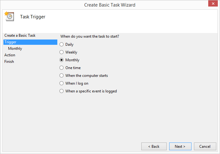
When you click Next, the task wizard will transition to the Monthly tab (see Figure 8-5). On the Monthly tab, you specify when you want the task to start. Because we’ve decided we want our script to run on a monthly basis, let’s select the last day of the current month and 9:00 AM as the start date. Check the “Synchronize across time zones” box, and select all months in the year (the “January, February, March...” option) and the “Last” day of each month. Once you’ve made these selections, click Next.
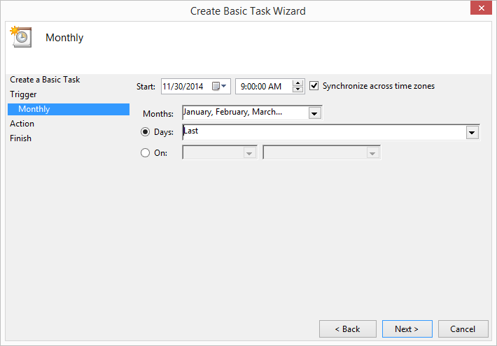
When you click Next, the task wizard will transition to the Action tab (see Figure 8-6). On the Action tab, you select the action you want the task to perform. Because we’ve decided we want our task to run a Python script, let’s select the “Start a program” radio button. Once you’ve selected the “Start a program” radio button, click Next.
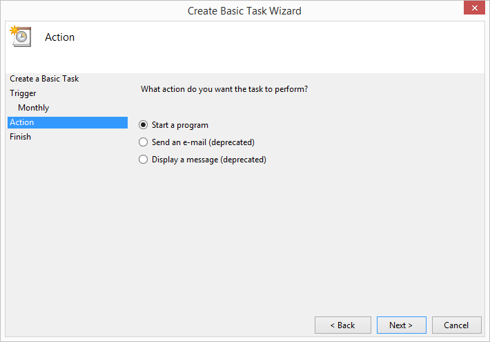
When you click Next, the task wizard will transition to the Start a Program tab (see Figure 8-7). On the Start a Program tab, you specify the program/script you want the task to start. Use the Browse button to locate the 3parse_text_file.py script on your Desktop. In addition, our script takes two command-line arguments, the name of the input file, mysql_server_error_log.txt, and the name of the output file, mysql_errors_count.csv. Supply these two arguments in the “Add arguments (optional)” box. Once you’ve entered the path to the Python script and the names of the input and output files, click Next.
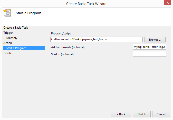
When you click Next, the task wizard will transition to the Finish tab (see Figure 8-8). The Finish tab summarizes all of the information you’ve entered into the task wizard so you can check that the information is correct before scheduling the task. Review the information in the Name, Description, Trigger, and Action fields to ensure that it is correct. Once you’ve verified that everything looks good, go ahead and click Finish.
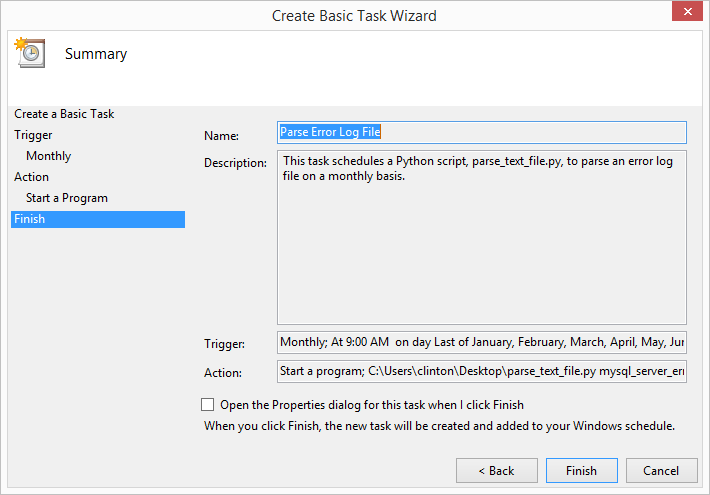
When you click Finish, the task wizard will add your task to the Task Scheduler Library and return to the Task Scheduler main screen (see Figure 8-9). To view your newly scheduled task, click on Task Scheduler Library in the upper-left corner of the main screen. When you click on Task Scheduler Library, you’ll see your new task listed, possibly among other tasks, in the upper center pane. If you click on the name of your new task in the upper center pane, you’ll then see summary tabs of information about your task (e.g., General, Triggers, Actions, etc.) in the lower center pane. Finally, if you want to edit or delete your task, click on your task in the upper center pane and then click Properties or Delete, respectively, in the upper-right corner of the main screen.
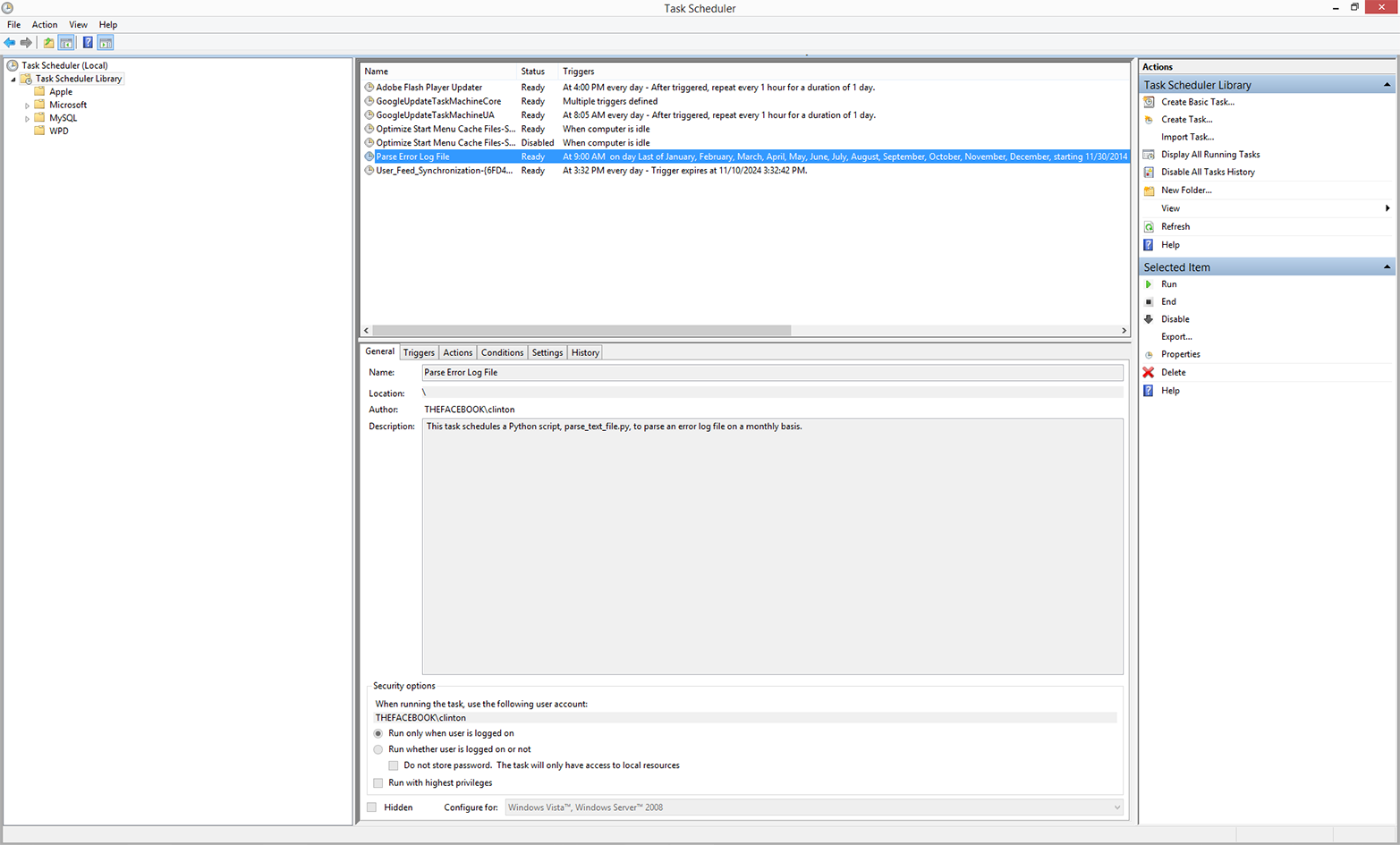
By scheduling Python scripts and other executable files to run on a regular basis automatically, you mitigate the possibility of forgetting to run a script manually. In addition, you can scale more effectively with automated scripts than by running scripts manually—i.e., as your business processes increasingly rely on scripts for data processing and analysis, it becomes progressively more difficult to run the scripts manually.
As you’ve seen, Windows provides the Task Scheduler program as a way to schedule scripts and other executable programs to run automatically on a regular basis. On macOS and Unix, the analogous program is called cron.
The cron program relies on a crontab file and cron jobs to know when to run particular executable programs. A crontab file is a plain-text file you create to list all of the executable files you want to schedule to run automatically along with the details about when each of the files should be run. A cron job is a single line item in the crontab file that specifies an executable file to be run (e.g., 3parse_text_file.py) and when to run the file (e.g., monthly).
The specific syntax for a cron job listing in the crontab file can be intimidating at first. The first five positions in the line specify the frequency with which to run the executable file. The positions from left to right are minute (0–59), hour (0–23), day of month (1–31), month (1–12), and day of week (0–6, where Sunday is 0). The final position in the line specifies the executable file that should be run with the specified frequency.
There are a few ways to specify valid values in the first five positions. If you want the executable file to be run for all of the values in a position, then you specify an asterisk (*) in the position. For example, if you want the file to be run every day of the month, then you place an asterisk in position three. Alternatively, if you want the file to be run at a specific time, then you specify particular values in the first two positions. For example, if you want the file to be run at 3:10 PM, then you place 10 in the first position and 15 in the second position (i.e., 12:00 PM + 3 hours = 15).
A good way to understand how to specify cron jobs is to view several examples. The following examples illustrate three possible cron job listings in a crontab file:
1015***/Users/clinton/Desktop/analyze_orders.py06,12,18**1-5/Users/clinton/Desktop/update_database.py3020**6/Users/clinton/Desktop/delete_temp_files.sh
The first row specifies that analyze_orders.py should be run every day of every month at 3:10 PM. The second row specifies that update_database.py should be run every weekday (Monday–Friday) of every month at 6:00 AM, 12:00 PM, and 6:00 PM. The third row specifies that delete_temp_files.sh (a Bash script) should be run every Saturday of every month at 8:30 PM.
These three examples illustrate some common cron job listings; however, you may need to run a script with a different frequency. For example, you may need to run a script on the first Monday of every month. When you know how frequently you need to run a script, but you’re unsure of how to specify it in the cron job listing, search for the specific syntax on the Internet (someone else has already discovered the solution for you). For example, a quick search for “cron job first Monday of month” shows that the following syntax will run the specified Python script, every_first_monday.py, on every first Monday of the month at 11:00 AM:
00111-7**["$(date '+\%a')"="Mon"]&&\/Users/clinton/every_first_monday.py
Now that we understand crontab files and cron jobs conceptually, let’s create a crontab file and specify a cron job to run our Python file, 3parse_text_file.py, on a regular basis.
Ensuring that you have a crontab file is basically a one-time setup. After you create a crontab file, you don’t need to recreate it again in the future. You can simply add, modify, or remove cron jobs in your existing crontab file to reflect the set of executable files you want to be run automatically on a regular basis.
To create a new, empty crontab file, open a Terminal window and use the following command:
touch crontab_file.txt
To load the crontab file (i.e., to get the operating system to load it and execute its instructions on its schedule), type the following on the command line and hit Enter:
crontab crontab_file.txt
Finally, remove crontab_file.txt from where you created it. To do so, simply type the following on the command line and hit Enter:
rm crontab_file.txt
That’s it—that’s all there is to creating an empty crontab file. We’ve completed our one-time setup. The screenshot in Figure 8-10 shows the three one-time setup commands, as well as the crontab -e command, which is for editing the crontab file.
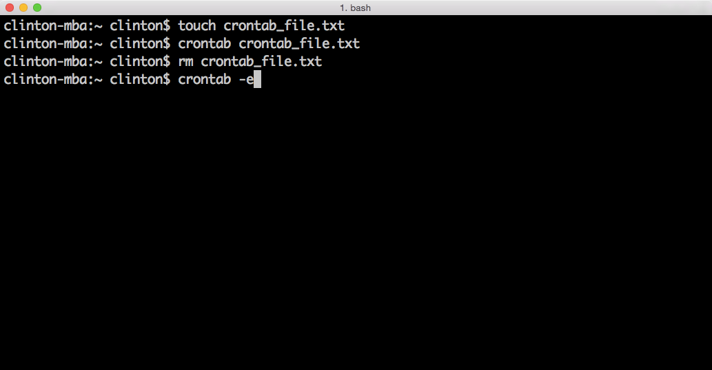
Now let’s add a cron job to the crontab file. To open a crontab file for editing, type the following and then hit Enter:
crontab -e
When you type crontab -e, your crontab file will open in a Unix-based text editor like Nano, vi/Vim, or Emacs. If your file opens in Nano or Emacs, you can immediately type the cron job command on the current line, hit Enter to move the cursor down to the next empty line, and then use the appropriate key sequence (described momentarily) to save your changes and exit out of the file.
On the other hand, if your file opens in vi/Vim, then you’ve entered an editor that has two modes of operation: a command mode and an insert mode. The file will open in command mode, meaning the next set of keys you type are commands that act on the file rather than enter text into the file. To switch from command mode to insert mode (which will allow you to add text into the file), type i. Once in insert mode, you can type the cron job command on the current line, hit Enter to move the cursor down to the next empty line, and then use the appropriate key sequence to save your changes and exit out of the file.
With the crontab file open, type the following command on the current line and then hit Enter to move the cursor down to the next empty line (see Figure 8-11):
00 09 28-31 * * [ "$(date -v+1d '+\%d')" = "01" ] &&\ /Users/clinton/Desktop/3parse_text_file.py
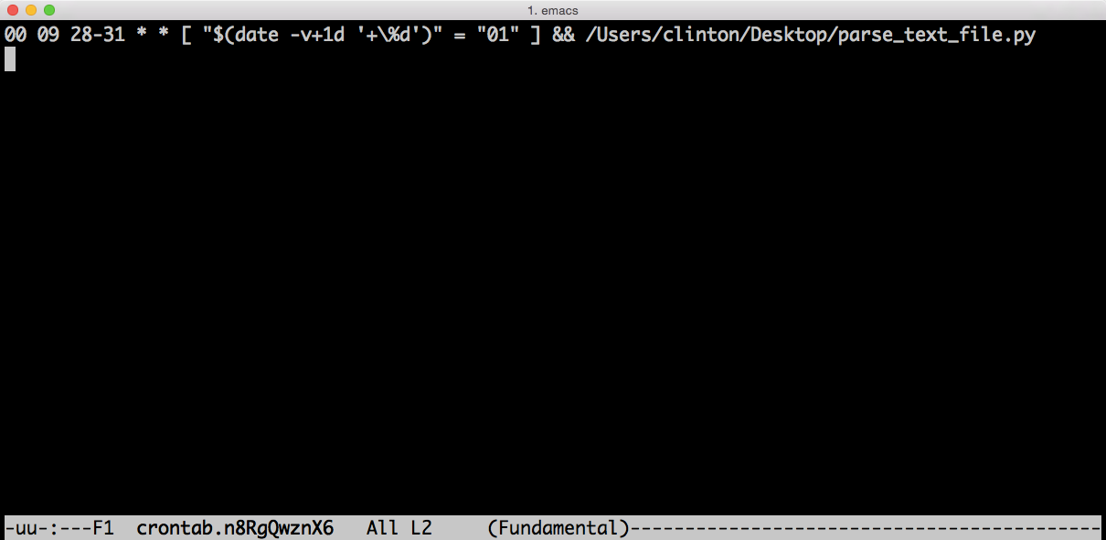
The command is consistent with the parameters we specified in Task Scheduler on Windows to run the script at 9:00 AM on the last day of every month. The first five positions on the lefthand side indicate that this job should run at 9:00 AM on the 28th, 29th, 30th, or 31st day of the month, depending on whether the next statement in square brackets is also true. The statement in square brackets tests whether adding one day to the current date results in the day of the month being 01 (i.e., the first day of the next month). This statement ensures that the script runs on the last day of the month, regardless of whether that day is the 28th in February, the 30th in June, or the 31st in October. The cron program checks the frequency parameters and the statement, and if the statement is true the cron job executes 3parse_text_file.py. This happens at 9:00 AM on the last day of every month.
Note that the cursor (denoted by the vertical white rectangle) is on the next empty line after the command you entered. Your crontab file can list many cron jobs, one on each line, but you must hit Enter after your last cron job listing so that the cursor ends up on the last empty line in the file.
Now that you’ve entered the cron job command in your crontab file, it’s time to save your changes to the file and exit out of the file. Depending on which editor you’re using, type one of the following command sequences to save your changes and exit out of the crontab file:
Nano: Ctrl+o, Ctrl+x
vi/Vim :, w, q
Emacs Ctrl+x, Ctrl+s, Ctrl+x, Ctrl+c
Now that you’ve saved your changes and exited out of the crontab file, let’s view the contents of the crontab file to see that the new cron job has been saved in the file. To view the contents of the crontab file, type the following command and then hit Enter (see Figure 8-12):
crontab -l
When you hit Enter, you’ll see the contents of your crontab file printed to the screen. As the screenshot shows, the crontab file contains our cron job command to run the 3parse_text_file.py script at 9:00 AM on the last day of every month.
To edit or delete a cron job, type crontab -e to open the crontab file. If you want to edit a cron job, simply make changes to the cron job command on the specific row you want to change. If you want to delete a cron job, simply delete the row that contains the cron job command you want to delete. In either case, make sure the cursor ends up on the last, empty row in the file. Then use the appropriate key sequence, depending on your text editor, to save your changes and exit out of the crontab file.
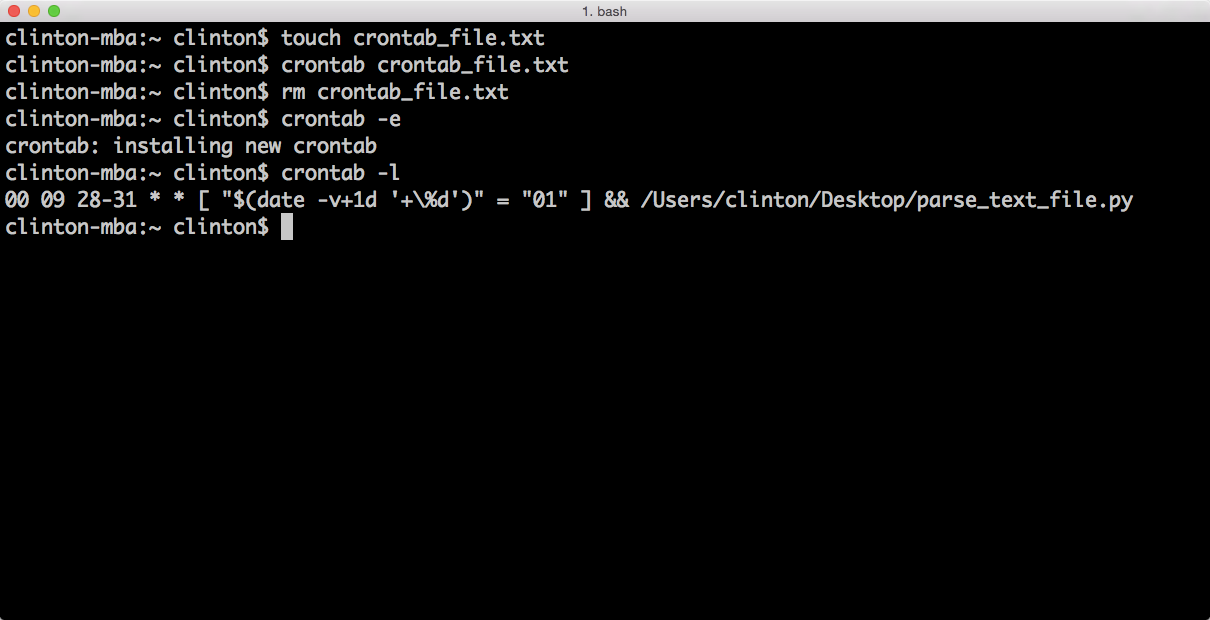
Even if you’re a regular Windows user, it’s important to know how to schedule cron jobs. You may be asked to schedule one at some point, and it’s useful to know how to implement automation on different operating systems.
This chapter has been shorter than the others, but it’s an important, complementary addition to the book, as the information here enables you to automate the running of scripts that you need to run on a regular basis. The other chapters gave you tools and techniques for scaling data processing and analysis, and this chapter enhanced that knowledge by enabling you to both scale and automate. By automating the running of scripts that need to be run on a regular basis, you mitigate the possibility of forgetting to run a script and you free your time to work on other important tasks.
Well, we’ve come to the final chapter in the book. We’ve covered a lot of material up to this point. We’ve covered Python basics and how to parse any number of text files, CSV files, Excel files, and data in databases. We’ve learned how to select specific rows and columns from these data sources, how to aggregate and calculate basic statistics using the data, and how to write the results to output files. We’ve tackled three common business analysis applications that require us to use the skills and techniques we’ve learned in creative and useful ways. We’ve also learned how to create some of the most common statistical plots with several add-in packages and how to estimate regression and classification models with the StatsModels package. Finally, we’ve learned how to schedule our scripts to run automatically on a regular basis so we have time to work on other interesting analytical problems. If you’ve followed along with and carried out all of the examples in this book, then I hope you feel like you’ve transitioned from non-programmer to competent hacker.
At this point, you might be wondering where you go from here. That is, what else is there to learn about using Python to scale and automate data analysis? In this chapter, I’ll mention some additional capabilities of the standard Python distribution that are interesting and useful but weren’t necessary for you to learn at the very beginning. Having gone through the preceding chapters in this book, hopefully you will find these additional capabilities easier to understand and handy extensions to the techniques you’ve learned so far.
I’ll also discuss the NumPy, SciPy, and Scikit-Learn add-in packages, because they provide foundational data containers and vectorized operations, scientific and statistical distributions and tests, and statistical modeling and machine learning functions that other packages such as pandas rely on and which go beyond those in the StatsModels package. For example, Scikit-Learn provides helpful functions for preprocessing data; reducing the dimensionality of the data; estimating regression, classification, and clustering models; comparing and selecting among competing models; and performing cross-validation. These methods help you create, test, and select models that will be robust to new data so that any predictions based on the models and new data are likely to be accurate.
Lastly, I am also going to discuss some additional data structures that are helpful to learn about as you become more proficient with Python. This book focused on list, tuple, and dictionary data structures because they are powerful, fundamental data containers that will meet your needs as a beginning programmer (and may be sufficient for your entire experience with Python). However, there are other data structures, like stacks, queues, heaps, trees, graphs, and others, that you will likely prefer to use for specific purposes.
We have explored many of Python’s built-in and standard library modules and functions that facilitate reading, writing, and analyzing data in text files, CSV files, Excel files, and databases. For example, we’ve used Python’s built-in csv, datetime, re, string, and sys modules. We’ve also used some of Python’s built-in functions, such as float, len, and sum.
However, we’ve really only scratched the surface of all of the modules and functions in Python’s standard library. In fact, there are some additional modules and functions I want to mention here because they are useful for data processing and analysis. These modules and functions didn’t make it into earlier chapters because either they didn’t fit into a specific example or they are advanced options, but it’s helpful to know that these modules and functions are available in case they can help with your specific analysis task. If you want to set yourself a challenge, try to learn at least one new skill from this list every day or every other day.
collections (PSL 8.3.)dict, list, set, and tuple. Some of the containers that tend to be used in data analyses are deque, Counter, defaultdict, and OrderedDict.random (PSL 9.3.)statistics (PSL 9.7.)itertools (PSL 10.1.)operator (PSL 10.3.)These five additional standard modules are a small subset of all of the modules available in Python’s standard library. In fact, there are over 35 sections in the standard library, each providing a wide variety of modules and functions related to specific topics. Because all of these modules are built into Python, you can use them immediately with an import statement, like from itertools import accumulate or from statistics import mode. To learn more about these and other standard modules, peruse the Python Standard Library.
Similar to the standard modules just discussed, there are also a few built-in functions that didn’t make it into earlier chapters but are still useful for data processing and analysis. As with the modules, it’s useful to know that these functions are available in case they can help with your specific analysis task. It’s helpful to have the following functions in your Python toolbox:
enumerate()index, value) tuplesfilter()zip()These functions are built into Python, so you can use them immediately. To learn more about these and other built-in functions, peruse the Python list of standard functions. In addition, it always helps to see how people use these functions to accomplish specific analysis tasks. If you’re interested in learning how others have used these functions, perform a quick Google or Bing search like “python enumerate examples” or “python zip examples” to retrieve a set of helpful examples.
As we’ve seen, the standard Python installation comes with a tremendous amount of built-in functionality. There are modules for accessing text and CSV files, manipulating text and numbers, and calculating statistics, as well as a whole host of other capabilities that we’re not covering in this book.
However, we’ve also seen that add-in modules, like xlrd, matplotlib, MySQL-python, pandas, and statsmodels provide additional functionality that isn’t available in Python’s standard library. In fact, there are several important, data-focused add-in modules that, once downloaded and installed, provide significant functionality for data visualization, data manipulation, statistical modeling, and machine learning. A few of these are NumPy, SciPy, Scikit-Learn, xarray (formerly xray), SKLL, NetworkX, PyMC, NLTK, and Cython.
These add-in modules, along with many others, are available for download at the Python Package Index website. In addition, Windows users who need to differentiate between 32-bit and 64-bit operating systems can find 32-bit and 64-bit versions of many of the add-in packages at the Unofficial Windows Binaries for Python Extension Packages website.
NumPy (pronounced “Num Pie”) is a foundational Python package that provides the ndarray, a fast, efficient, multidimensional data container for (primarily) numerical data. It also provides vectorized versions of standard mathematical and statistical functions that enable you to operate on arrays without for loops. Some of the helpful functions NumPy provides include functions for reading, reshaping, aggregating, and slicing and dicing structured data (especially numerical data).
As is the case with pandas, which is built on top of NumPy, many of NumPy’s functions encapsulate and simplify techniques you’ve learned in this book. NumPy is a fundamental package that underlies many other add-in packages (and provides the powerful ndarray data structure with vectorized operations), so let’s review some of NumPy’s functionality.
In Chapter 2, we discussed how to use the built-in csv module to read and write CSV files. To read a CSV file, we used a with statement to open the input file and a filereader object to read all of the rows in the file. Similarly, to write a CSV file, we used a with statement to open the output file and a filewriter object to write to the output file. In both cases, we also used a for loop to iterate through and process all of the rows in the input file.
NumPy simplifies reading and writing CSV and text files with three functions: loadtxt, genfromtxt, and savetxt. By default, the loadtxt function assumes the data in the input file consists of floating-point numbers separated by some amount of whitespace; however, you can include additional arguments in the function to override these default values.
Instead of the file-reading code we discussed in Chapter 2, if your dataset does not include a header row and the values are floating-point numbers separated by spaces, then you can write the following statements to load your data into a NumPy array and immediately have access to all of your data:
fromnumpyimportloadtxtmy_ndarray=loadtxt('input_file.csv')(my_ndarray)
From here, you can perform a lot of data manipulations similar to the ones we’ve discussed in this book. To provide another example, imagine you have a file, people.txt, which contains the following data:
nameagecolorscoreclint32green15.6john30blue22.3rachel27red31.4
Notice that this dataset contains a header row and columns that are not floating-point numbers. In this case, you can use the skiprows argument to skip the header row and specify separate data types for each of the columns:
fromnumpyimportdtype,loadtxtperson_dtype=dtype([('name','S10'),('age',int),('color','S6'),\('score',float)])people=loadtxt('people.txt',skiprows=1,dtype=person_dtype)(people)
By creating person_dtype, you’re creating a structured array in which the values in the name column are strings with a maximum length of 10 characters, the values in the age column are integers, the values in the color column are strings, and the values in the score column are floating-point numbers.
In this example the columns are space-delimited, but if your data is comma-delimited you can use delimiter=',' in the loadtxt function to indicate that the columns are comma-delimited.
The genfromtxt function attempts to simplify your life even further by automatically determining the data types in the columns. As with loadtxt, the genfromtxt function provides additional arguments you can use to facilitate reading different types of file formats and data into structured arrays.
For example, you can use the names argument to indicate that there’s a header row and you can use the converters argument to change and format the data you read in from the input file:
fromnumpyimportgenfromtxtname_to_int=dict(rachel=1,john=2,clint=3)color_to_int=dict(blue=1,green=2,red=3)defconvert_name(n):returnname_to_int.get(n,-999)defconvert_color(c):returncolor_to_int.get(c,-999)data=genfromtxt('people.txt',dtype=float,names=True,\converters={0:convert_name,2:convert_color})(data)
In this example, I want to convert the values in the name and color columns from strings to floating-point numbers. For each column, I create a dictionary mapping the original string values to numbers. I also define two helper functions that retrieve the numeric values in the dictionaries for each name and color, or return –999 if the name or color doesn’t appear in the dictionary.
In the genfromtxt function, the dtype argument indicates that all of the values in the resulting dataset will be floating-point numbers, the names argument indicates that genfromtxt should look for the column headings in the first row, and the converters argument specifies a dictionary that maps column numbers to the converter functions that will convert the data in these columns.
For example, imagine you have a CSV file, myCSVInputFile.csv, which contains the following data:
2.1,3.2,4.33.2,4.3,5.24.3,2.6,1.5
You can read this data into a list of lists using the techniques we discussed in this book and then convert the list into a NumPy array:
importcsvfromnumpyimportarrayfile=open('myCSVInputFile.csv','r')file_reader=csv.reader(file)data=[]forrow_listinfile_reader:row_list_floats=[float(value)forvalueinrow_list]data.append(row_list_floats)file.close()data=array(data)(data)
Alternatively, if you have an Excel file, you can use the pandas read_excel function to read the data into a DataFrame and then convert the object into a NumPy array:
frompandasimportread_excelfromnumpyimportarraymyDataFrame=read_excel('myExcelInputFile.xlsx')data=array(myDataFrame)(data)
NumPy provides the savetxt function for saving data to CSV and other text files. First you specify the name of the output file and then you specify the data you want to save to the file:
fromnumpyimportsavetxtsavetxt('output_file.txt',data)
By default, savetxt saves the data using scientific format. You don’t always want to save data using scientific format, so you can use the fmt argument to specify the format you want to use. You can also include the delimiter argument to specify the column delimiter:
savetxt('output_file.txt',data,fmt='%d')savetxt('output_file.csv',data,fmt='%.2f',delimiter=',')
Also, by default savetxt doesn’t include a header row. If you want a header row in the output file, you can provide a string to the header argument. By default, savetxt includes the hash symbol (#) before the first column header to make the row a comment. You can turn off this behavior by setting the comments argument equal to the empty string:
column_headings_list=['var1','var2','var3']header_string=','.join(column_headings_list)savetxt('output_file.csv',data,fmt='%.2f',delimiter=',',\comments='',header=header_string)
Once you’ve created a structured NumPy array, you can filter for specific rows using filtering conditions similar to the ones you would use in pandas. For example, assuming you’ve created a structured array named data that contains at least the columns Cost, Supplier, Quantity, and Time to Delivery, you can filter for specific rows using conditions like the following:
row_filter1=(data['Cost']>110)&(data['Supplier']==3)data[row_filter1]row_filter2=(data['Quantity']>55)|(data['Time to Delivery']>30)data[row_filter2]
The first filtering condition filters for rows where the value in the Cost column is greater than 110 and the value in the Supplier column equals 3. Similarly, the second filtering condition filters for rows where the value in the Quantity column is greater than 55 or the value in the Time to Delivery column is greater than 30.
Selecting a subset of columns in a structured array can be challenging because of data type differences between the columns in the subset. You can define a helper function to provide a view of the subset of columns and handle the subset’s data types:
importnumpyasnpdefcolumns_view(arr,fields):dtype2=np.dtype({name:arr.dtype.fields[name]fornameinfields})returnnp.ndarray(arr.shape,dtype2,arr,0,arr.strides)
Then you can use the helper function to view a subset of columns from the structured array. You can also specify row-filtering conditions to filter for specific rows and select specific columns at the same time, similar to using the ix function in pandas:
supplies_view=columns_view(supplies,['Supplier','Cost'])(supplies_view)row_filter=supplies['Cost']>1000supplies_row_column_filters=columns_view(supplies[row_filter],\['Supplier','Cost'])(supplies_total_cost_gt_1000_two_columns)
NumPy simplifies the process of concatenating data from multiple arrays with its concatenate, vstack, r_, hstack, and c_ functions. The concatenate function is more general than the others. It takes a list of arrays and concatenates them together according to an additional axis argument, which specifies whether the arrays should be concatenated vertically (axis=0) or horizontally (axis=1). The vstack and r_ functions are specifically for concatenating arrays vertically, and the hstack and c_ functions are specifically for concatenating arrays horizontally. For example, here are three ways to concatenate arrays vertically:
importnumpyasnpfromnumpyimportconcatenate,vstack,r_array_concat=np.concatenate([array1,array2],axis=0)array_concat=np.vstack((array1,array2))array_concat=np.r_[array1,array2]
These three functions produce the same results. In each case, the arrays listed inside the function are concatenated vertically, on top of one another. If you assign the result to a new variable as I do here, then you have a new larger array that contains all of the data from the input arrays.
Similarly, here are three ways to concatenate arrays horizontally:
importnumpyasnpfromnumpyimportconcatenate,hstack,c_array_concat=np.concatenate([array1,array2],axis=1)array_concat=np.hstack((array1,array2))array_concat=np.c_[array1,array2]
Again, these three functions produce the same results. In each case, the arrays listed inside the function are concatenated horizontally, side by side.
This section has presented some of NumPy’s features and capabilities, but there are many more that you should check out. One important difference between NumPy and base Python is that NumPy enables vectorized operations, which means you can apply operations to entire arrays element by element without needing to use a for loop.
For example, if you have two arrays, array1 and array2, and you need to add them together element by element you can simply write array_sum = array1 + array2. This operation adds the two arrays element by element, so the result is an array where the value in each position is the sum of the values in the same position in the two input arrays. Moreover, the vectorized operations are executed in C code, so they are carried out very quickly.
Another helpful feature of NumPy is a collection of statistical calculation methods that operate on arrays. Some of the statistical calculations are sum, prod, amin, amax, mean, var, std, argmin, and argmax. sum and prod calculate the sum and product of the values in an array. amin and amax identify the minimum and maximum values in an array. mean, var, and std calculate the mean, variance, and standard deviation of the values in an array. argmin and argmax find the index position of the minimum and maximum values in an array. All of the functions accept the axis argument, so you can specify whether you want the calculation down a column (axis=0) or across a row (axis=1).
For more information about NumPy, and to download it, visit the NumPy website.
SciPy (pronounced “Sigh Pie”) is another foundational Python package that provides scientific and statistical distributions, functions, and tests for mathematics, science, and engineering. SciPy has a broad scope, so its functionality is organized into different subpackages. Some of the subpackages are:
clusterconstantsinterpolateiolinalgsparsespatialstatsweaveAs you can see from this list, SciPy’s subpackages provide functionality for a diverse range of operations and calculations. For example, the linalg package provides functions for performing very fast linear algebra operations on two-dimensional arrays; the interpolate package provides functions for linear and curvilinear interpolation between data points; and the stats package provides functions for working with random variables, calculating descriptive and test statistics, and conducting regression.
SciPy is a fundamental package that underlies many other add-in packages (in addition to providing a variety of useful mathematical and statistical functions), so let’s review some of SciPy’s functionality.
The linalg package provides functions for all of the basic linear algebra routines, including finding inverses, finding determinants, and computing norms. It also has functions for matrix decompositions and exponential, logarithm, and trigonometric functions. Some other useful functions enable you to quickly solve linear systems of equations and linear least-squares problems.
SciPy provides the linalg.solve function for computing the solution vector of a linear system of equations. Suppose we need to solve the following system of simultaneous equations:
x + 2y + 3z = 3
2x + 3y + z = –10
5x – y + 2z = 14
We can represent these equations with a coefficient matrix, a vector of unknowns, and a righthand-side vector. The linalg.solve function takes the coefficient matrix and the righthand-side vector and solves for the unknowns (i.e., x, y, and z):
fromnumpyimportarrayfromscipyimportlinalgA=array([[1,2,3],[2,3,1],[5,-1,2]])b=array([[3],[-10],[14]])solution=linalg.solve(A,b)(solution)
The values for x, y, and z that solve the system of equations are: 0.1667, –4.8333, and 4.1667.
SciPy provides the linalg.lstsq function for computing the solution vector of a linear least-squares problem. In econometrics, it’s common to see a linear least-squares estimated model expressed in matrix notation as:
y = Xb + e
where y is a vector for the dependent variable, X is a matrix of coefficients for the independent variables, b is the solution vector of values to be estimated, and e is a vector of residuals computed from the data. The linalg.lstsq function takes the coefficient matrix, X, and the dependent variable, y, and solves for the solution vector, b:
importnumpyasnpfromscipyimportlinalgc1,c2=6.0,3.0i=np.r_[1:21]xi=0.1*iyi=c1*np.exp(-xi)+c2*xizi=yi+0.05*np.max(yi)*np.random.randn(len(yi))A=np.c_[np.exp(-xi)[:,np.newaxis],xi[:,np.newaxis]]c,resid,rank,sigma=linalg.lstsq(A,zi)(c)
Here, c1, c2, i, and xi simply serve to construct yi, the initial formulation of the dependent variable. However, the next line constructs zi, the variable that actually serves as the dependent variable, by adding some random disturbances to the yi values. The lstsq function returns values for c, residuals (resid), rank, and sigma. The two c values that solve this least-squares problem are 5.92 and 3.07.
The interpolate package provides functions for linear and curvilear interpolation between known data points. The function for univariate data is named interp1d, and the function for multivariate data is named griddata. The package also provides functions for spline interpolation and radial basis functions for smoothing and interpolation. The interp1d function takes two arrays and returns a function that uses interpolation to find the values of new points:
fromnumpyimportarange,expfromscipyimportinterpolateimportmatplotlib.pyplotaspltx=arange(0,20)y=exp(-x/4.5)interpolation_function=interpolate.interp1d(x,y)new_x=arange(0,19,0.1)new_y=interpolation_function(new_x)plt.plot(x,y,'o',new_x,new_y,'-')plt.show()
The blue dots in the plot are the 20 original data points. The green line connects the interpolated values of new points between the original data points. Because I didn’t specify the kind argument in the interp1d function, it used the default linear interpolation to find the values. However, you can also specify quadratic, cubic, or a handful of other string or integer values to specify the type of interpolation it should perform.
The stats package provides functions for generating values from specific distributions, calculating descriptive statistics, performing statistical tests, and conducting regression analysis. The package offers over eighty continuous random variables and ten discrete random variables. It has tests for analyzing one sample and tests for comparing two samples. It also has functions for kernel density estimation, or estimating the probability density function of a random variable from a set of data.
The stats package provides several functions for calculating descriptive statistics:
fromscipy.statsimportnorm,describex=norm.rvs(loc=5,scale=2,size=1000)(x.mean())(x.min())(x.max())(x.var())(x.std())x_nobs,(x_min,x_max),x_mean,x_variance,x_skewness,x_kurtosis=describe(x)(x_nobs)
In this example, I create an array, x, of 1,000 values drawn from a normal distribution with mean equal to five and standard deviation equal to two. The mean, min, max, var, and std functions compute the mean, minimum, maximum, variance, and standard deviation of x, respectively. Similarly, the describe function returns the number of observations, the minimum and maximum values, the mean and variance, and the skewness and kurtosis.
The stats package simplifies the process of estimating the slope and intercept in a linear regression. In addition to the slope and intercept, the linregress function also returns the correlation coefficient, the two-sided p-value for a null hypothesis that the slope is zero, and the standard error of the estimate:
fromnumpy.randomimportrandomfromscipyimportstatsx=random(20)y=random(20)slope,intercept,r_value,p_value,std_err=stats.linregress(x,y)("R-squared:",round(r_value**2,4))
In this example, the print statement squares the correlation coefficient to display the R-squared value.
The preceding examples only scratched the surface of the subpackages and functions that are available in the SciPy package. For more information about SciPy, and to download it, visit the SciPy website.
The Scikit-Learn add-in module provides functions for estimating statistical machine learning models, including regression, classification, and clustering models, as well as data preprocessing, dimensionality reduction, and model selection. Scikit-Learn’s functions handle both supervised models, where the dependent variable’s values or class labels are available, and unsupervised models, where the values or class labels are not available. One of the features of Scikit-Learn that distinguishes it from StatsModels is a set of functions for conducting different types of cross-validation (i.e., testing a model’s performance on data that was not used to fit the model).
Testing a model’s performance on the same data that was used to fit the model is a methodological mistake because it is possible to create models that repeat the dependent variable’s values or class labels perfectly with the data used to fit the model. These models might appear to have excellent performance based on their results with the data at hand, but they’re actually overfitting the model data and would not have good performance or provide useful predictions on new data.
To avoid overfitting and estimate a model that will tend to have good performance on new data, it is common to split a dataset into two pieces, a training set and a test set. The training set is used to formulate and fit the model, and the test set is used to evaluate the model’s performance. Because the data used to fit the model is different than the data used to evaluate the model’s performance, the chances of overfitting are reduced. This process of repeatedly splitting a dataset into two pieces—training a model on the training set and testing the model on the test set—is called cross-validation.
There are many different methods of cross-validation, but one basic method is called k-fold cross-validation. In k-fold cross-validation, the original dataset is split into a training set and a test set and then the training set is again split into k pieces, or “folds” (e.g., five or ten folds). Then, for each of the k folds, k – 1 of the folds are used as training data to fit the model and the remaining fold is used to evaluate the model’s performance. In this way, cross-validation creates several performance values, one for each fold, and the final performance measure for the training set is the average of the values calculated for each fold. Finally, the cross-validated model is run on the test data to calculate the overall performance measure for the model.
To see how straightforward it is to formulate statistical learning models in Scikit-Learn, let’s specify a random forest model with cross-validation. If you are not familiar with random forest models, check out the Wikipedia entry for an overview or, for a more in-depth treatment, see The Elements of Statistical Learning by Trevor Hastie, Robert Tibshirani, and Jerome Friedman or Applied Predictive Modeling by Max Kuhn and Kjell Johnson (both from Springer), which are excellent resources on the topic. You can formulate a random forest model with cross-validation and evaluate the model’s performance with a few lines of code in Scikit-Learn:
importnumpyasnpimportpandasaspdfromsklearn.preprocessingimportStandardScalerfromsklearn.cross_validationimportKFoldfromsklearn.ensembleimportRandomForestClassifierasRFy=data_frame['Purchased?']y_pred=y.copy()feature_space=data_frame[numeric_columns]X=feature_space.as_matrix().astype(np.float)scaler=StandardScaler()X=scaler.fit_transform(X)kf=KFold(len(y),n_folds=5,shuffle=True,random_state=123)fortrain_index,test_indexinkf:X_train,X_test=X[train_index],X[test_index]y_train=y[train_index]clf=RF()clf.fit(X_train,y_train)y_pred[test_index]=clf.predict(X_test)accuracy=np.mean(y==y_pred)"Random forest: "+"%.3f"%(accuracy)
The first five lines of code import NumPy, pandas, and three components of Scikit-Learn. In order, the three components enable you to center and scale the explanatory variables, carry out k-fold cross-validation, and use the random forest classifier.
The next block of code handles specifying the dependent variable, y; creating the matrix of explanatory variables, X; and centering and scaling the explanatory variables. This block assumes that you’ve already created a pandas DataFrame called data_frame and the data for the dependent variable is in a column called Purchased?. The copy function makes a copy of the dependent variable, assigning it into y_pred, which will be used to evaluate the model’s performance. The next line assumes you’ve created a list of the numeric variables in data_frame so you can select them as your set of explanatory variables. The following line uses NumPy and pandas functions to transform the feature set into a matrix called X. The last two lines in the block use Scikit-Learn functions to create and use a scaler object to center and scale the explanatory variables.
The next block of code implements k-fold cross-validation with the random forest classifier. The first line uses the KFold function to split the dataset into five different pairs, or folds, of training and test sets. The next line is a for loop for iterating through each of the folds. Within the for loop, for each fold, we assign the training and test sets of explanatory variables, assign the training set for the dependent variable, initialize the random forest classifier, fit the random forest model with the training data, and then use the model and test data to estimate predicted values for the dependent variable.
The final block of code calculates and reports the model’s accuracy. The first line uses NumPy’s mean function to calculate the average number of times the predicted values for the dependent variable equal the actual, original data values. The evaluation in parentheses tests whether the two values are equal (i.e., whether they are both 1 or are both 0), so the mean function averages a series of 1s and 0s. If all of the predicted values match the original data values, then the average will be 1. If all of the predicted values do not match the original values, then the average will be 0. Therefore, we want the cross-validated random forest classifier to produce an average value that is close to 1. The final line prints the model’s accuracy, formatted to three decimal places, to the screen.
This example illustrated how to carry out cross-validation with a random forest classifier model in Scikit-Learn. Scikit-Learn enables you to specify many more regression and classification models than were presented in this section. For example, to implement a support vector machine, all you would need to do is add the following import statement (and change the classifier from clf = RF() to clf = SVC()):
fromsklearn.svmimportSVC
In addition to other models, Scikit-Learn also has functions for data pre-processing, dimensionality reduction, and model selection.
To learn more about Scikit-Learn and how to estimate other models and use other cross-validation methods in Scikit-Learn, check out the Scikit-Learn documentation.
In addition to NumPy, SciPy, and Scikit-Learn, there are a few additional add-in packages that you may want to look into, depending on the type of data analysis you need to do. This list represents a tiny fraction of the thousands of add-in Python packages on the Python Package Index and is simply intended as a suggestion of some packages that you might find intriguing and useful:
These packages do not come preinstalled with Python. You have to download and install them separately. To do so, visit the Python Package Index website or the Unofficial Windows Binaries for Python Extension Packages website.
As you move on from this book and start to solve various business data processing and analysis tasks with Python, it will become increasingly important for you to become familiar with some additional data structures. By learning about these concepts, you’ll expand your toolkit to include a broader understanding of the various ways it is possible to implement a solution and be able to evaluate the trade-offs between different options. You’ll also become savvy about what data structures to use in a specific circumstance to store, process, or analyze your data more quickly and efficiently.
Additional data structures that are helpful to know about include stacks, queues, graphs, and trees. In certain circumstances, these data structures will store and retrieve your data more efficiently and with better memory utilization than lists, tuples, or dictionaries.
A stack is an ordered collection of items where you add an item to and remove an item from the same end of the stack. You can only add or remove one item at a time. The end where you add and remove items is called the top. The opposite end is called the base. Given a stack’s ordering principle, items near the top have been in the stack for less time than items near the base. In addition, the order in which you remove items from the stack is opposite to the order in which you add them. This property is called LIFO (last in, first out).
Consider a stack of trays in a cafeteria. To create the stack, you place a tray on the counter, then you place another tray on top of the first tray, and so on. To shrink the stack, you take a tray from the top of the stack. You can add or remove a tray at any time, but it must always be added to or removed from the top.
There are lots of data processing and analysis situations in which it’s helpful to use stacks. People implement stacks to allocate and access computer memory, to store command-line and function arguments, to parse expressions, to reverse data items, and to store and backtrack through URLs.
A queue is an ordered collection of items where you add items to one end of the queue and remove items from the other end of the queue. In a queue, you add items to the rear and they make their way to the front, where they are removed. Given a queue’s ordering principle, items near the rear have been in the queue for less time than items near the front. This property is called FIFO (first in, first out).
Consider any well-maintained queue, or line, you’ve ever waited in. Regardless of whether you’re at a theme park, a movie theater, or a grocery store, you enter the queue at the back and then wait until you make your way to the front of the queue, where you receive your ticket or service; then you leave the queue.
There are lots of data processing and analysis situations in which it’s helpful to use queues. People implement queues to process print jobs on a printer, to hold computer processes waiting for resources, and to optimize queues and network flows.
A graph is a set of nodes (a.k.a. vertices) and edges, which connect to nodes. The edges can be directed, representing a direction between two nodes, or undirected, representing a connection between two nodes with no particular direction. They can also have weights that represent some relationship between the two nodes, which depends on the context of the problem.
Consider any graphical representation of the relationship between people, places, or topics. For example, imagine a collection of actors, directors, and movies as nodes on a canvas and edges between the nodes indicating who acted in or directed the movies. Alternatively, imagine cities as nodes on a canvas and the edges between the nodes indicating the paths to get from one city to the next. The edges can be weighted to indicate the distance between two cities.
There are lots of data processing and analysis situations in which it’s helpful to use graphs. People implement graphs to represent relationships among suppliers, customers, and products; to represent relationships between entities; to represent maps; and to represent capacity and demand for different resources.
A tree is a specific type of graph data structure consisting of a hierarchical set of nodes and edges. In a tree, there is a single topmost node, which is designated as the root node. The root node may have any number of child nodes. Each of these nodes may also have any number of child nodes. A child node may only have one parent node. If each node has a maximum of two child nodes, then the tree is called a binary tree.
Consider elements in HTML. Within the html tags there are head and body tags. Within the head tag, there may be meta and title tags. Within the body tag, there may be h1, div, form, and ul tags. Viewing these tags in a tree structure, you see the html tag as the root node with two child nodes, the head and body tags. Under the node for the head tag, you see meta and title tags. Under the node for the body tag, you see h1, div, form, and ul tags.
There are lots of data processing and analysis situations in which it’s helpful to use trees. People implement trees to create computer filesystems, to manage hierarchical data, to make information easy to search, and to represent the phrase structure of sentences.
This section presented a very brief introduction some classic data structures. A nice resource for learning more about these data structures in Python is Brad Miller and David Ranum’s online book, Problem Solving with Algorithms and Data Structures Using Python.
It’s helpful to know that these data containers exist so you have the option to use them when your initial implementation isn’t performing well. By knowing about these data structures and understanding when to use one type versus another, you’ll be able to solve a variety of large, difficult problems and improve the processing time and memory utilization of many of your scripts.
If when you started reading this book you had never programmed before, then you’ve picked up a lot of foundational programming experience as you followed along with the examples. We started by downloading Python, writing a basic Python script in a text editor, and figuring out how to run the script on Windows and macOS. After that, we developed a first script to explore many of Python’s basic data types, data containers or structures, control flow, and how to read and write text files. From there, we learned how to parse specific rows and columns in CSV files; how to parse specific worksheets, rows, and columns in Excel files; and how to load data, modify data, and write out data in databases. In Chapter 3 and Chapter 4, we downloaded MySQL and some extra Python add-in modules. Once we had all of that experience under our belts, in Chapter 5 we applied and extended our new programming skills to tackle three real-world applications. Then, in Chapter 6 and Chapter 7, we transitioned from data processing to data visualization and statistical analysis. Finally, in Chapter 8, we learned how to automate our scripts so they run on a routine basis without us needing to run them manually from the command line. Having arrived at the end of the book, you may be thinking, “Where should I go from here?”
At this point in my own training, I received some valuable advice: “Identify an important or interesting specific problem/task that you think could be improved with Python and work on it until you accomplish what you set out to do.” You want to choose an important or interesting problem so you’re excited about the project and invested in accomplishing your goal. You’re going to hit stumbling blocks, wrong turns, and dead ends along the way, so the project has to be important enough to you that you persevere through the difficult patches and keep writing, debugging, and editing until your code works. You also want to select a specific problem or task so that what you need your code to do is clearly defined. For example, your situation may be that you have too many files to process manually, so you need to figure out how to process them with Python. Or perhaps you’re responsible for a specific data processing or analysis task and you think the task could be automated and made more efficient and consistent with Python. Once you have a specific problem or task in mind, it’s easier to think about how to break it down into the individual operations that need to happen to accomplish your goal.
Once you’ve chosen a specific problem or task and outlined the operations that need to happen, you’re in a really good position. It’s easier to figure out how to accomplish one particular operation than it is to envision how to accomplish the whole task at once. The quote I’m thinking of here is, “How do you devour a whale? One bite at a time.” The nice thing about tackling one particular operation at a time is that, for each operation, it’s highly likely that someone else has already tackled that problem, figured it out, and shared his or her code online or in a book.
The Internet is your friend, especially when it comes to code. We’ve already covered how to read CSV and Excel files in this book, but what if you need to read a different type of file, such as a JSON or HTML file? Open a browser and enter something like “python read json file examples” in the search bar to see how other people have read JSON files in Python. The same advice goes for all of the other operations you’ve outlined for your problem or task. In addition to online resources, which are very helpful once you’ve narrowed down to a specific operation, there are also many books and training materials on Python that contain helpful code snippets and examples. You can find many free PDF versions of Python books online, and many are also available through your local and county libraries. My point is that you don’t have to reinvent the wheel. For each small operation in your overall problem or task, use whatever code you can from this book, search online and in other resources to see how others have tackled the operation, and then edit and debug until you get it working. What you’ll end up with, after you’ve tackled each of the individual operations, is a Python script that solves your specific problem or task. And that’s the exciting moment you’re working toward: that moment when you press a button and the code you’ve labored over for days or weeks to get working carries out your instructions and solves your problem or task for you—the feeling is exhilarating and empowering. Once you realize that you can efficiently accomplish tasks that would be tedious, time consuming, error prone, or impossible to do manually, you’ll feel a rush of excitement and be looking for more problems and tasks to solve with Python. That’s what I hope for you—that you go on from here and work on a problem or task that’s important to you until your code works and you accomplish what you set out to do.
Go to https://www.python.org/downloads (the downloads page detects your operating system and suggests the Windows version).
Click Download Python 3.4.3 (or the newest version of Python 3—it may have been updated since the time of this book’s publication).
Click “Windows x86 MSI installer” to save or run the MSI installer.
Double-click the downloaded python-3.4.3.msi installer to open the Python Installer.
Select “Install for all users” or “Install just for me” and then click Next.
Use the default destination directory (C:\Python34\), and click Next.
For all of the remaining screens, click Next without changing the default values.
Python should now be installed.
Once Python is installed:
Click Start.
Click Control Panel.
Click System and Security.
Click System.
Click “Advanced system settings.”
Click the Advanced tab.
Click the Environment Variables option.
Under the “System variables” option, scroll down to and click on the Path variable.
Click Edit.
In the “Variable value” field, check to make sure C:\Python34\ is included in the list.
If it is not in the list, scroll to the end of the list and type “;C:\Python34\” at the end of the list to add the path to the list (the semicolon is used to separate individual paths).
Click OK to save your changes to the Path system variable.
Click OK to exit the Environment Variables window.
Click OK to exit the System Properties window.
Now click File Explorer.
Double-click the C: drive.
Double-click the Python34 folder.
Double-click the python application.
If the Python Shell window opens, then you are good to go.
Click iTerm to open a Terminal window.
Type the following and then hit Enter:
which python
If you see a path like /usr/bin/python or /usr/local/bin/python displayed in the Terminal window, then Python is already installed and you are good to go.
If you do not see a path like /usr/bin/python or /usr/local/bin/python, then follow these instructions to install Python:
Go to https://www.python.org/downloads (the downloads page detects your operating system and suggests the Mac OS version).
Click Download Python 3.4.3 (or the newest version of Python 3—it may have been updated since the time of this book’s publication).
Click Save File to download python-3.4.3-macosx10.6.pkg.
Double-click python-3.4.3-macosx10.6.pkg to open the Python Installer.
Click Continue to move past the Welcome screen.
Click Continue to move past the Important Information screen.
Click Agree/Continue to move past the Software License Agreement screen.
Click Install to install Python in the default destination directory.
For all of the remaining screens, click Continue without changing the default values.
Python should now be installed.
Click Applications to open your applications.
Click iTerm to open a Terminal window.
Type the following and then hit Enter:
which python
You should now see a path like /usr/bin/python or /usr/local/bin/python, indicating that Python has been installed and you are good to go.
Before completing these steps, you first need to install Python 3.
Open a Command Prompt window.
Type the following and then hit Enter:
python -m pip install xlrd
After you hit Enter, you should see output printed in the Command Prompt window indicating that the xlrd package has been installed.
To confirm that xlrd installed properly:
Click File Explorer.
Double-click the C: drive.
Double-click the Python34 folder.
Double-click the python application.
When the Python Shell window opens, type the following and hit Enter:
import xlrd
If you don’t receive any error messages, then xlrd installed properly and you are good to go.
Click the green Downloads button to download the latest version of xlrd.
Right-click on the downloaded application and select “Show in folder.”
Unzip the folder in your Downloads folder.
Double-click the unzipped xlrd-0.9.3.tar folder to enter the folder.
Click on and copy the unzipped xlrd-0.9.3 folder.
Go back out to your Downloads folder and paste the unzipped xlrd-0.9.3 folder into that folder.
Open a Command Prompt window.
To move into your Downloads folder, type the following and hit Enter:
cd Downloads
To move into the unzipped xlrd-0.9.3 folder, type the following and hit Enter:
cd xlrd-0.9.3
Now that you are inside the xlrd-0.9.3 folder, type the following and hit Enter:
python setup.py install
After you hit Enter, you should see output printed in the Command Prompt window indicating that the xlrd package has been installed.
To confirm that xlrd installed properly:
Click File Explorer.
Double-click the C: drive.
Double-click the Python34 folder.
Double-click the python application.
When the Python Shell window opens, type the following and hit Enter:
import xlrd
If you don’t receive any error messages, then xlrd installed properly and you are good to go.
Before completing these steps, you first need to install Python 3.
Click Applications to open your applications.
Click iTerm to open a Terminal window.
Type the following and then hit Enter:
python -m pip install xlrd
After you hit Enter, you should see output printed in the Terminal window indicating that the xlrd package has been installed.
If instead you receive an error, try typing the following and then hitting Enter:
sudo python -m pip install xlrd
You’ll be asked to enter the password you use to log in to your computer. Type your password (it won’t appear on the screen) and then hit Enter.
To confirm that xlrd installed properly:
Click Applications to open your applications.
Click iTerm to open a Terminal window.
To open the Python interpreter inside the Terminal window, type the following and then hit Enter:
python
Once the Python interpreter opens, type the following and then hit Enter:
import xlrd
If you don’t receive any error messages, then xlrd installed properly and you are good to go.
Click the green Downloads button to move down to the downloadable files.
Click “xlrd-0.9.3.tar.gz” (or the newest version—it may have been updated since the time of publication) to save the zipped file in your Downloads folder.
Double-click the downloaded file to unzip it in the Downloads folder.
If you have any trouble unzipping the file you can also unzip it from the Terminal window. Type the following in a Terminal window and then hit Enter to move into the Downloads folder:
cd Downloads
Next, to unzip the file, type the following and then hit Enter:
tar -zxvf xlrd-0.9.3.tar.gz
Now the unzipped folder xlrd-0.9.3 should be in your Downloads folder.
Click Applications to open your applications.
Click iTerm to open a Terminal window.
To move into your Downloads folder, type the following and hit Enter:
cd Downloads/
To move into the unzipped xlrd-0.9.3 folder, type the following and then hit Enter:
cd xlrd-0.9.3/
Now that you are inside the xlrd-0.9.3 folder, type the following and then hit Enter:
python setup.py install
After you hit Enter, you should see output printed in the Terminal window indicating that the xlrd package has been installed.
If instead you receive an error, try typing the following and then hitting Enter:
sudo python setup.py install
You’ll be asked to enter the password you use to log in to your computer. Type your password (it won’t appear on the screen) and then hit Enter.
To confirm that xlrd installed properly:
Click Applications to open your applications.
Click iTerm to open a Terminal window.
To open the Python interpreter inside the Terminal window, type the following and then hit Enter:
python
Once the Python interpreter opens, type the following and then hit Enter:
import xlrd
If you don’t receive any error messages, then xlrd installed properly and you are good to go.
Click MySQL Community Server.
Click the Download button next to “Mac OS X 10.11 (x86, 64-bit), DMG Archive.”
Be sure to select the .dmg archive, which comes with its own installer.
Click “No thanks, just start my download.”
When the download is finished, click on the downloaded installer.
Follow the installer’s instructions.
I won’t lie to you: this can be hairy. The MySQL Reference Manual has a section on installing that will get you a good part of the way there, but you may well need to Google an error message or two along the way.
Before completing these steps, you’ll probably first need to download MySQL; the installer for the Python packages will check for MySQL’s configuration files as it’s setting up and will fail if it doesn’t find MySQL.
Before completing these steps, you first need to install Python 3.
Open a Command Prompt window.
Type the following and then hit Enter:
python -m pip install mysqlclient
After you hit Enter, you should see output printed in the Command Prompt window indicating that the mysqlclient package has been installed.
To confirm that mysqlclient installed properly:
Click File Explorer.
Double-click the C: drive.
Double-click the Python34 folder.
Double-click the python application.
When the Python Shell window opens, type the following and then hit Enter:
import MySQLdb
If you don’t receive any error messages, then mysqlclient installed properly and you are good to go.
Go to http://www.lfd.uci.edu/~gohlke/pythonlibs/#mysqlclient.
Click the link for the version of mysqlclient that corresponds to your version of Python (i.e., 3.x or 2.x) and your operating system (i.e., 32-bit or 64-bit).
Save the file in your Downloads folder.
You can determine the version you need by opening a Command Prompt window, typing python and hitting Enter to enter the Python interpreter, and reviewing the header information at the top of the screen. You should see details like “Python 3.4.3 (32-bit),” which indicates that you need to select the link for 32-bit Python 3.4. At the time of this writing, the link is: mysqlclient-1.3.6-cp34-none-win32.whl. If you have a different version of Python or a different type of operating system, then you need to select the link that corresponds to your information.
Open a Command Prompt window.
Type the following and then hit Enter:
cd Downloads
Type the following (substituting a different filename if necessary) and then hit Enter:
python -m pip install mysqlclient-1.3.6-cp34-none-win32.whl
After you hit Enter, you should see output printed in the Command Prompt window indicating that the mysqlclient package has been installed.
To confirm that mysqlclient installed properly:
Click File Explorer.
Double-click the C: drive.
Double-click the Python34 folder.
Double-click the python application.
When the Python Shell window opens, type the following and then hit Enter:
import mysqlclient
If you don’t receive any error messages, then mysqlclient installed properly and you are good to go.
Before completing these steps, you first need to install Python 3.
Click Applications to open your applications.
Click iTerm to open a Terminal window.
Type the following and then hit Enter:
python -m pip install mysqlclient
After you hit Enter, you should see output printed in the Terminal window indicating that the mysqlclient package has been installed.
If instead you receive an error, try typing the following and then hitting Enter:
sudo python -m pip install mysqlclient
You’ll be asked to enter the password you use to log in to your computer. Type your password (it won’t appear on the screen) and then hit Enter.
To confirm that mysqlclient installed properly:
Click Applications to open your applications.
Click iTerm to open a Terminal window.
To open the Python interpreter inside the Terminal window, type the following and then hit Enter:
python
Once the Python interpreter opens, type the following and then hit Enter:
import mysqlclient
If you don’t receive any error messages, then mysqlclient installed properly and you are good to go.
Click the green Downloads button to move down to the downloadable files.
Click “mysqlclient-1.3.6.tar.gz” (or the newest version—it may have been updated since the time of publication) to save the zipped file in your Downloads folder.
Double-click the downloaded file to unzip it in the Downloads folder.
If you have any trouble unzipping the file, you can also unzip it from the Terminal window. Type the following in a Terminal window and then hit Enter to move into the Downloads folder:
cd Downloads
Next, to unzip the file, type the following and hit Enter:
tar -zxvf mysqlclient-1.3.6.tar.gz
Now the unzipped folder mysqlclient-1.3.6 should be in your Downloads folder.
Click Applications to open your applications.
Click iTerm to open a Terminal window.
To move into your Downloads folder, type the following and hit Enter:
cd Downloads/
To move into the unzipped mysqlclient-1.3.6 folder, type the following and then hit Enter:
cd mysqlclient-1.3.6/
Now that you are inside the mysqlclient-1.3.6 folder, type the following and then hit Enter:
python setup.py install
After you hit Enter, you should see output printed in the Terminal window indicating that the mysqlclient package has been installed.
If instead you receive an error, try typing the following and then hitting Enter:
sudo python setup.py install
You’ll be asked to enter the password you use to log in to your computer. Type your password (it won’t appear on the screen) and then hit Enter.
To confirm that mysqlclient installed properly:
Click Applications to open your applications.
Click iTerm to open a Terminal window.
To open the Python interpreter inside the Terminal window, type the following and then hit Enter:
python
Once the Python interpreter opens, type the following and then hit Enter:
import mysqlclient
If you don’t receive any error messages, then mysqlclient installed properly and you are good to go.
#!/usr/bin/env python3farm_animals=['cow','pig','horse']domestic_animals=['dog','cat','gold fish']zoo_animals=['lion','elephant','gorilla']animals=farm_animals+domestic_animals+zoo_animalsforindex_valueinrange(len(animals)):("{0:d}: {1!s}".format(index_value,animals[index_value]))
#!/usr/bin/env python3animals_dictionary={}animals_list=['cow','pig','horse']other_list=[4567,[4,'turn',7,'left'],'Animals are great.']forindex_valueinrange(len(animals_list)):ifanimals_list[index_value]notinanimals_dictionary:animals_dictionary[animals_list[index_value]]=other_list[index_value]forkey,valueinanimals_dictionary.items():("{0!s}: {1}".format(key,value))
#!/usr/bin/env python3list_of_lists=[['cow','pig','horse'],['dog','cat','gold fish'],\['lion','elephant','gorilla']]foranimal_listinlist_of_lists:max_index=len(animal_list)output=''forindexinrange(len(animal_list)):ifindex<(max_index-1):output+=str(animal_list[index])+','else:output+=str(animal_list[index])+'\n'(output)
Gelman, Andrew and Jennifer Hill. Data Analysis Using Regression and Multilevel/Hierarchical Models. New York: Cambridge University Press, 2007. Print.
Harms, Daryl and Kenneth McDonald. The Quick Python Book. Greenwich, CT: Manning Publications, 2000. Print.
McKinney, Wes. Python for Data Analysis. Sebastopol, CA: O’Reilly Media, 2012. Print.
Miller, Brad and David Ranum. Problem Solving with Algorithms and Data Structures using Python. Auckland: Runstone Interactive Python, 2005. Online.
The animal on the cover of Foundations for Analytics with Python is an oleander moth caterpillar (Syntomeida epilais).
Oleander caterpillars are orange with tufts of black hairs; they largely feed on oleander, an evergreen shrub that is the most poisonous commonly grown garden plant. The caterpillar is immune to the plant’s poison and by ingesting it, becomes toxic to any bird or mammal that tries to eat it. When the oleander was introduced to Florida by the Spanish in the 17th century, the moth already existed in Florida using a native vine as its host plant, but as oleander became more available, the moth adapted to the new plant as its host to such an extent that it became known as the oleander moth.
The adult oleander moth is spectacular: the body and wings are iridescent blue with small white dots, and the abdomen is bright red at its tip. These moths are active during daylight hours, slow-flying, and imitate the shape of wasps. Female moths perch on oleander foliage and emit an ultrasonic acoustic signal that attracts male moths from great distances. When male and female moths are within a few meters of each other, they begin a courtship duet of acoustic calls that continues until mating occurs two or three hours before dawn. Once mated, female moths oviposit on the undersides of the leaves of oleander plants. Egg masses can contain from 12 to 75 eggs. Once hatched, the larvae gregariously feed on the plant tissue between the major and minor leaf veins until the shoot is a brown skeleton. This defoliation does not kill the plant but it does leave it susceptible to other pests.
Many of the animals on O’Reilly covers are endangered; all of them are important to the world. To learn more about how you can help, go to animals.oreilly.com.
The cover image is from Wood’s Illustrated Natural History. The cover fonts are URW Typewriter and Guardian Sans. The text font is Adobe Minion Pro; the heading font is Adobe Myriad Condensed; and the code font is Dalton Maag’s Ubuntu Mono.
For Aisha and Amaya,
“Education is the kindling of a flame,
not the filling of a vessel.” —Socrates
May you always enjoy stoking the fire.
Copyright © 2016 Clinton Brownley. All rights reserved.
Printed in the United States of America.
Published by O’Reilly Media, Inc., 1005 Gravenstein Highway North, Sebastopol, CA 95472.
O’Reilly books may be purchased for educational, business, or sales promotional use. Online editions are also available for most titles (http://oreilly.com/safari). For more information, contact our corporate/institutional sales department: 800-998-9938 or corporate@oreilly.com.
See http://oreilly.com/catalog/errata.csp?isbn=9781491922538 for release details.
The O’Reilly logo is a registered trademark of O’Reilly Media, Inc. Foundations for Analytics with Python, the cover image, and related trade dress are trademarks of O’Reilly Media, Inc.
While the publisher and the author have used good faith efforts to ensure that the information and instructions contained in this work are accurate, the publisher and the author disclaim all responsibility for errors or omissions, including without limitation responsibility for damages resulting from the use of or reliance on this work. Use of the information and instructions contained in this work is at your own risk. If any code samples or other technology this work contains or describes is subject to open source licenses or the intellectual property rights of others, it is your responsibility to ensure that your use thereof complies with such licenses and/or rights.
978-1-491-92253-8
[LSI]
This book is intended for readers who deal with data in spreadsheets on a regular basis, but who have never written a line of code. The opening chapters will get you set up with the Python environment, and teach you how to get the computer to look at data and take simple actions with it. Soon, you’ll learn to do things with data in spreadsheets (CSV files) and databases.
At first this will feel like a step backward, especially if you’re a power user of Excel. Painstakingly telling Python how to loop through every cell in a column when you used to select and paste feels slow and frustrating (especially when you have to go back three times to find a typo). But as you become more proficient, you’ll start to see where Python really shines, especially in automating tasks that you currently do over and over.
This book is written so that you can work through it from beginning to end and feel confident that you can write code that works and does what you expect at the end. It’s probably a good idea to type out the code at first, so that you get accustomed to things like tabs and closing your parentheses and quotes, but all the code is available online and you may wind up referring to those links to copy and paste as you do your own work in the future. That’s fine! Knowing when to cut and paste is part of being an efficient programmer. Reading the book as you go through the examples will teach you why and how the code samples work.
Good luck on your journey to becoming a programmer!
If you deal with data on a regular basis, then there are a lot of reasons for you to be excited about learning how to program. One benefit is that you can scale your data processing and analysis tasks beyond what would be feasible or practical to do manually. Perhaps you’ve already come across the problem of needing to process large files that contain so much data that it’s impossible or impractical to open them. Even if you can open the files, processing them manually is time consuming and error prone, because any modifications you make to the data take a long time to update—and with so much data, it’s easy to miss a row or column that you intended to change. Or perhaps you’ve come across the problem of needing to process a large number of files—so many files that it’s impossible or impractical to process them manually. In some cases, you need to use data from dozens, hundreds, or even thousands of files. As the number of files increases, it becomes increasingly difficult to handle them manually. In both of these situations, writing a Python script to process the files solves your problem because Python scripts can process large files and lots of files quickly and efficiently.
Another benefit of learning to program is that you can automate repetitive data manipulation and analysis processes. In many cases, the operations we carry out on data are repetitive and time consuming. For example, a common data management process involves receiving data from a customer or supplier, extracting the data you want to retain, possibly transforming or reformatting the data, and then saving the data in a database or other data repository (this is the process known to data scientists as ETL—extract, transform, load). Similarly, a typical data analysis process involves acquiring the data you want to analyze, preparing the data for analysis, analyzing the data, and reporting the results. In both of these situations, once the process is established, it’s possible to write Python code to carry out the operations. By creating a Python script to carry out the operations, you reduce a time-consuming, repetitive process down to the running of a script and free up your time to work on other impactful tasks.
On top of that, carrying out data processing and analysis operations in a Python script instead of manually reduces the chance of errors. When you process data manually, it’s always possible to make a copy/paste error or a typo. There are lots of reasons why this might happen—you might be working so quickly that you miss the mistake, or you might be distracted or tired. Furthermore, the chance of errors increases when you’re processing large files or lots of files, or when you’re carrying out repetitive actions. Conversely, a Python script doesn’t get distracted or tired. Once you debug your script and confirm that it processes the data the way you want it to, it will carry out the operations consistently and tirelessly.
Finally, learning to program is fun and empowering. Once you’re familiar with the basic syntax, it’s fun to try to figure out which pieces of syntax you need and how to fit them together to accomplish your overall data analysis goal. When it comes to code and syntax, there are lots of examples online that show you how to use specific pieces of syntax to carry out particular tasks. Online examples give you something to work with, but then you need to use your creativity and problem-solving skills to figure out how you need to modify the code you found online to suit your needs. The whole process of searching for the right code and figuring out how to make it work for you can be a lot of fun. Moreover, learning to program is incredibly empowering. For example, consider the situations I mentioned before, involving large files or lots of files. When you can’t program, these situations are either incredibly time consuming or simply infeasible. Once you can program, you can tackle both situations relatively quickly and easily with Python scripts. Being able to carry out data processing and analysis tasks that were once laborious or impossible provides a tremendous rush of positive energy, so much so that you’ll be looking for more opportunities to tackle challenging data processing tasks with Python.
This book is written for people who deal with data on a regular basis and have little to no programming experience. The examples in this book cover common data sources and formats, including text files, comma-separated values (CSV) files, Excel files, and databases. In some cases, these files contain so much data or there are so many files that it’s impractical or impossible to open them or deal with them manually. In other cases, the process used to extract and use the data in the files is time consuming and error prone. In these situations, without the ability to program, you have to spend a lot of your time searching for the data you need, opening and closing files, and copying and pasting data.
Because you may never have run a script before, we’ll start from the very beginning, exploring how to write code in a text file to create a Python script. We’ll then review how to run our Python scripts in a Command Prompt window (for Windows users) and a Terminal window (for macOS users). (If you’ve done a bit of programming, you can skim Chapter 1 and move right into the data analysis parts in Chapter 2.)
Another way I’ve set out to make this book very user-friendly for new programmers is that instead of presenting code snippets that you’d need to figure out how to combine to carry out useful work, the examples in this book contain all of the Python code you need to accomplish a specific task. You might find that you’re coming back to this book as a reference later on, and having all the code at hand will be really helpful then. Finally, following the adage “a picture is worth a thousand words,” this book uses screenshots of the input files, Python scripts, Command Prompt and Terminal windows, and output files so you can literally see how to create the inputs, code, commands, and outputs.
I’m going to go into detail to show how things work, as well as giving you some tools that you can put to use. This approach will help you build a solid basis for understanding “what’s going on under the hood”—there will be times when you Google a solution to your problem and find useful code, and having done the exercises in this book, you’ll have a good understanding of how code you find online works. This means you’ll know both how to apply it in your situation and how to fix it if it breaks. As you’ll build working code through these chapters, you may find that you’ll use this book as a reference, or a “cookbook,” with recipes to accomplish specific tasks. But remember, this is a “learn to cook” book; you’ll be developing skills that you can generalize and combine to do all sorts of tasks.
The majority of examples in this book show how to create and run Python scripts on Microsoft Windows. The focus on Windows is fairly straightforward: I want this book to help as many people as possible, and according to available estimates, the vast majority of desktop and laptop computers—especially in business analytics—run a Windows operating system. For instance, according to Net Applications, as of December 2014, Microsoft Windows occupies approximately 90% of the desktop and laptop operating system market. Because I want this book to appeal to desktop and laptop users, and the vast majority of these computers have a Windows operating system, I concentrate on showing how to create and run Python scripts on Windows.
Despite the book’s emphasis on Windows, I also provide examples of how to create and run Python scripts on macOS, where appropriate. Almost everything that happens within Python itself will happen the same way no matter what kind of machine you’re running it on. But where there are differences between operating systems, I’ll give specific instructions for each. For instance, the first example in Chapter 1 illustrates how to create and run a Python script on both Microsoft Windows and macOS. Similarly, the first examples in Chapters 2 and 3 also illustrate how to create and run the scripts on both Windows and macOS. In addition, Chapter 8 covers both operating systems by showing how to create scheduled tasks on Windows and cron jobs on macOS. If you are a Mac user, use the first example in each chapter as a template for how to create a Python script, make it executable, and run the script. Then repeat the steps to create and run all of the remaining examples in each chapter.
There are many reasons to choose Python if your aim is to learn how to program in a language that will enable you to scale and automate data processing and analysis tasks. One notable feature of Python is its use of whitespace and indentation to denote line endings and blocks of code, in contrast to many other languages, which use extra characters like semicolons and curly braces for these purposes. This makes it relatively easy to see at first glance how a Python program is put together.
The extra characters found in other languages are troublesome for people who are new to programming, for at least two reasons. First, they make the learning curve longer and steeper. When you’re learning to program, you’re essentially learning a new language, and these extra characters are one more aspect of the language you need to learn before you can use the language effectively. Second, they can make the code difficult to read. Because in these other languages semicolons and curly braces denote blocks of code, people don’t always use indentation to guide your eye around the blocks of code. Without indentation, these blocks of code can look like a jumbled mess.
Python sidesteps these difficulties by using whitespace and indentation, not semicolons and curly braces, to denote blocks of code. As you look through Python code, your eyes focus on the actual lines of code rather than the delimiters between blocks of code, because everything around the code is whitespace. Python code requires blocks of code to be indented, and indentation makes it easy to see where one block of code ends and another begins. Moreover, the Python community emphasizes code readability, so there is a culture of writing code that is comparatively easy to read and understand. All of these features make the learning curve shorter and shallower, which means you can get up and running and processing data with Python relatively quickly compared to many alternatives.
Another notable feature of Python that makes it ideal for data processing and analysis is the number of standard and add-in modules and functions that facilitate common data processing and analysis operations. Built-ins and standard library modules and functions come standard with Python, so when you download and install Python you immediately have access to these built-in modules and functions. You can read about all of the built-ins and standard modules in the Python Standard Library (PSL). Add-ins are other Python modules that you download and install separately so you can use the additional functions they provide. You can peruse many of the add-ins in the Python Package Index (PyPI).
Some of the modules in the standard library provide functions for reading different file types (e.g., text, comma-separated values, JSON, HTML, XML, etc.); manipulating numbers, strings, and dates; using regular expression pattern matching; parsing comma-separated values files; calculating basic statistics; and writing data to different output file types and to disk. There are too many useful add-in modules to cover them all, but a few that we’ll use or discuss in this book include the following:
xlrd and xlwtmysqlclient/MySQL-python/MySQLdbpandasstatsmodelsscikit-learnIf you’re new to programming and you’re looking for a programming language that will enable you to automate and scale your data processing and analysis tasks, then Python is an ideal choice. Python’s emphasis on whitespace and indentation means the code is easier to read and understand, which makes the learning curve less steep than for other languages. And Python’s built-in and add-in packages facilitate many common data manipulation and analysis operations, which makes it easy to complete all of your data processing and analysis tasks in one place.
Pandas is an add-in module for Python that provides numerous functions for reading/writing, combining, transforming, and managing data. It also has functions for calculating statistics and creating graphs and plots. All of these functions simplify and reduce the amount of code you need to write to accomplish your data processing tasks. The module has become very popular among data analysts and others who use Python because it offers a lot of helpful functions, it’s fast and powerful, and it simplifies and reduces the code you have to write to get your job done. Given its power and popularity, I want to introduce you to pandas in this book. To do so, I present pandas versions of the scripts in Chapters 2 and 3, I illustrate how to create graphs and plots with pandas in Chapter 6, and I demonstrate how to calculate various statistics with pandas in Chapter 7. I also encourage you to pick up a copy of Wes McKinney’s book, Python for Data Analysis (O’Reilly).1
At the same time, if you’re new to programming, I also want you to learn basic programming skills. Once you learn these skills, you’ll develop generally applicable problem-solving skills that will enable you to break down complex problems into smaller components, solve the smaller components, and then combine the components together to solve the larger problem. You’ll also develop intuition for which data structures and algorithms you can use to solve different problems efficiently and effectively. In addition, there will be times when an add-in module like pandas doesn’t have the functionality you need or isn’t working the way you need it to. In these situations, if you don’t have basic programming skills, you’re stuck. Conversely, if you do have these skills you can create the functionality you need and solve the problem on your own. Being able to solve a programming problem on your own is exhilarating and incredibly empowering.
Because this book is for people who are new to programming, the focus is on basic, generally applicable programming skills. For instance, Chapter 1 introduces fundamental concepts such as data types, data containers, control flow, functions, if-else logic, and reading and writing files. In addition, Chapters 2 and 3 present two versions of each script: a base Python version and a pandas version. In each case, I present and discuss the base Python version first so you learn how to implement a solution on your own with general code, and then I present the pandas version. My hope is that you will develop fundamental programming skills from the base Python versions so you can use the pandas versions with a firm understanding of the concepts and operations pandas simplifies for you.
When it comes to Python, there are a variety of applications in which you can write your code. For example, if you download Python from Python.org, then your installation of Python comes with a graphical user interface (GUI) text editor called Idle. Alternatively, you can download IPython Notebook and write your code in an interactive, web-based environment. If you’re working on macOS or you’ve installed Cygwin on Windows, then you can write your code in a Terminal window using one of the built-in text editors like Nano, Vim, or Emacs. If you’re already familiar with one of these applications, then feel free to use it to follow along with the examples in this book.
However, in this section, I’m going to provide instructions for downloading and installing the free Anaconda Python distribution from Continuum Analytics because it has some advantages over the alternatives for a beginning programmer—and for the advanced programmer, too! The major advantage is that it comes with hundreds of the most popular add-in Python packages preinstalled so you don’t have to experience the inevitable headaches of trying to install them and their dependencies on your own. For example, all of the add-in packages we use in this book come preinstalled in Anaconda Python.
Another advantage is that it comes with an integrated development environment, or IDE, called Spyder. Spyder provides a convenient interface for writing, executing, and debugging your code, as well as installing packages and launching IPython Notebooks. It includes nice features such as links to online documentation, syntax coloring, keyboard shortcuts, and error warnings.
Another nice aspect of Anaconda Python is that it’s cross-platform—there are versions for Linux, Mac, and Windows. So if you learn to use it on Windows but need to transition to a Mac at a later point, you’ll still be able to use the same familiar interface.
One aspect of Anaconda Python to keep in mind while you’re becoming familiar with Python and all of the available add-in packages is the syntax you use to install add-in packages. In Anaconda Python, you use the conda install command. For example, to install the add-in package argparse, you would type conda install argparse. This syntax is different from the usual pip install command you’d use if you’d installed Python from Python.org (if you’d installed Python from Python.org, then you’d install the argparse package with python -m pip install argparse). Anaconda Python also allows you to use the pip install syntax, so you can actually use either method, but it’s helpful to be aware of this slight difference while you’re learning to install add-in packages.
To install Anaconda Python, follow these steps:
Go to http://continuum.io/downloads (the website automatically detects your operating system—i.e., Windows or Mac).
Select “Windows 64-bit Python 3.5 Graphical Installer” (if you’re using Windows) or “Mac OS X 64-bit Python 3.5 Graphical Installer” (if you’re on a Mac).
Double-click the downloaded .exe (for Windows) or .pkg (for Mac) file.
Follow the installer’s instructions.
Although we’ll be using Anaconda Python and Spyder in this book, it’s helpful to be familiar with some text editors that provide features for writing Python code. For instance, if you didn’t want to use Anaconda Python, you could simply install Python from Python.org and then use a text editor like Notepad (for Windows) or TextEdit (for macOS). To use TextEdit to write Python scripts, you need to open TextEdit and change the radio button under TextEdit→Preferences from “Rich text” to “Plain text” so new files open as plain text. Then you’ll be able to save the files with a .py extension.
An advantage of writing your code in a text editor is that there should already be one on your computer, so you don’t have to worry about downloading and installing additional software. And as most desktops and laptops ship with a text editor, if you ever have to work on a different computer (e.g., one that doesn’t have Spyder or a Terminal window), you’ll be able to get up and running quickly with whatever text editor is available on the computer.
While writing your Python code in a text editor such as Notepad or TextEdit is completely acceptable and effective, there are other free text editors you can download that offer additional features, including code highlighting, adjustable tab sizes, and multi-line indenting and dedenting. These features (particularly code highlighting and multi-line indenting and dedenting) are incredibly helpful, especially while you’re learning to write and debug your code.
Here is a noncomprehensive list of some free text editors that offer these features:
Notepad++ (Windows)
Sublime Text (Windows and Mac)
jEdit (Windows and Mac)
TextWrangler (Mac)
Again, I’ll be using Anaconda Python and Spyder in this book, but feel free to use a text editor to follow along with the examples. If you download one of these editors, be sure to search online for the keystroke combination to use to indent and dedent multiple lines at a time. It’ll make your life a lot easier when you start experimenting with and debugging blocks of code.
All of the Python scripts, input files, and output files presented in this book are available online at https://github.com/cbrownley/foundations-for-analytics-with-python.
It’s possible to download the whole folder of materials to your computer, but it’s probably simpler to just click on the filename and copy/paste the script into your text editor. (GitHub is a website for sharing and collaborating on code—it’s very good at keeping track of different versions of a project and managing the collaboration process, but it has a pretty steep learning curve. When you’re ready to start sharing your code and suggesting changes to other people’s code, you might take a look at Chad Thompson’s Learning Git (Infinite Skills).)
We’ll begin by exploring how to create and run a Python script. This chapter focuses on basic Python syntax and the elements of Python that you need to know for later chapters in the book. For example, we’ll discuss basic data types such as numbers and strings and how you can manipulate them. We’ll also cover the main data containers (i.e., lists, tuples, and dictionaries) and how you use them to store and manipulate your data, as well as how to deal with dates, as dates often appear in business analysis. This chapter also discusses programming concepts such as control flow, functions, and exceptions, as these are important elements for including business logic in your code and gracefully handling errors. Finally, the chapter explains how to get your computer to read a text file, read multiple text files, and write to a CSV-formatted output file. These are important techniques for accessing input data and retaining specific output data that I expand on in later chapters in the book.
This chapter covers how to read and write CSV files. The chapter starts with an example of parsing a CSV input file “by hand,” without Python’s built-in csv module. It transitions to an illustration of potential problems with this method of parsing and then presents an example of how to avoid these potential problems by parsing a CSV file with Python’s csv module. Next, the chapter discusses how to use three different types of conditional logic to filter for specific rows from the input file and write them to a CSV output file. Then the chapter presents two different ways to filter for specific columns and write them to the output file. After covering how to read and parse a single CSV input file, we’ll move on to discussing how to read and process multiple CSV files. The examples in this section include presenting summary information about each of the input files, concatenating data from the input files, and calculating basic statistics for each of the input files. The chapter ends with a couple of examples of less common procedures, including selecting a set of contiguous rows and adding a header row to the dataset.
Next, we’ll cover how to read Excel workbooks with a downloadable, add-in module called xlrd. This chapter starts with an example of introspecting an Excel workbook (i.e., presenting how many worksheets the workbook contains, the names of the worksheets, and the number of rows and columns in each of the worksheets). Because Excel stores dates as numbers, the next section illustrates how to use a set of functions to format dates so they appear as dates instead of as numbers. Next, the chapter discusses how to use three different types of conditional logic to filter for specific rows from a single worksheet and write them to a CSV output file. Then the chapter presents two different ways to filter for specific columns and write them to the output file. After covering how to read and parse a single worksheet, the chapter moves on to discuss how to read and process all worksheets in a workbook and a subset of worksheets in a workbook. The examples in these sections show how to filter for specific rows and columns in the worksheets. After discussing how to read and parse any number of worksheets in a single workbook, the chapter moves on to review how to read and process multiple workbooks. The examples in this section include presenting summary information about each of the workbooks, concatenating data from the workbooks, and calculating basic statistics for each of the workbooks. The chapter ends with a couple of examples of less common procedures, including selecting a set of contiguous rows and adding a header row to the dataset.
Here, we’ll cover how to carry out basic database operations in Python. The chapter starts with examples that use Python’s built-in sqlite3 module so that you don’t have to install any additional software. The examples illustrate how to carry out some of the most common database operations, including creating a database and table, loading data in a CSV input file into a database table, updating records in a table using a CSV input file, and querying a table. When you use the sqlite3 module, the database connection details are slightly different from the ones you would use to connect to other database systems like MySQL, PostgreSQL, and Oracle. To show this difference, the second half of the chapter demonstrates how to interact with a MySQL database system. If you don’t already have MySQL on your computer, the first step is to download and install MySQL. From there, the examples mirror the sqlite3 examples, including creating a database and table, loading data in a CSV input file into a database table, updating records in a table using a CSV input file, querying a table, and writing query results to a CSV output file. Together, the examples in the two halves of this chapter provide a solid foundation for carrying out common database operations in Python.
This chapter contains three examples that demonstrate how to combine techniques presented in earlier chapters to tackle three different problems that are representative of some common data processing and analysis tasks. The first application covers how to find specific records in a large collection of Excel and CSV files. As you can imagine, it’s a lot more efficient and fun to have a computer search for the records you need than it is to search for them yourself. Opening, searching in, and closing dozens of files isn’t fun, and the task becomes more and more challenging as the number of files increases. Because the problem involves searching through CSV and Excel files, this example utilizes a lot of the material covered in Chapters 2 and 3.
The second application covers how to group or “bin” data into unique categories and calculate statistics for each of the categories. The specific example is parsing a CSV file of customer service package purchases that shows when customers paid for particular service packages (i.e., Bronze, Silver, or Gold), organizing the data into unique customer names and packages, and adding up the amount of time each customer spent in each package. The example uses two building blocks, creating a function and storing data in a dictionary, which are introduced in Chapter 1 but aren’t used in Chapters 2, 3, and 4. It also introduces another new technique: keeping track of the previous row you processed and the row you’re currently processing, in order to calculate a statistic based on values in the two rows. These two techniques—grouping or binning data with a dictionary and keeping track of the current row and the previous row—are very powerful capabilities that enable you to handle many common analysis tasks that involve events over time.
The third application covers how to parse a text file, group or bin data into categories, and calculate statistics for the categories. The specific example is parsing a MySQL error log file, organizing the data into unique dates and error messages, and counting the number of times each error message appeared on each date. The example reviews how to parse a text file, a technique that briefly appears in Chapter 1. The example also shows how to store information separately in both a list and a dictionary in order to create the header row and the data rows for the output file. This is a reminder that you can parse text files with basic string operations and another good example of how to use a nested dictionary to group or bin data into unique categories.
In this chapter, you’ll learn how to create common statistical graphs and plots in Python with four plotting libraries: matplotlib, pandas, ggplot, and seaborn. The chapter begins with matplotlib because it’s a long-standing package with lots of documentation (in fact, pandas and seaborn are built on top of matplotlib). The matplotlib section illustrates how to create histograms and bar, line, scatter, and box plots. The pandas section discusses some of the ways pandas simplifies the syntax you need to create these plots and illustrates how to create them with pandas. The ggplot section notes the library’s historical relationship with R and the Grammar of Graphics and illustrates how to use ggplot to build some common statistical plots. Finally, the seaborn section discusses how to create standard statistical plots as well as plots that would be more cumbersome to code in matplotlib.
Here, we’ll look at how to produce standard summary statistics and estimate regression and classification models with the pandas and statsmodels packages. pandas has functions for calculating measures of central tendency (e.g., mean, median, and mode), as well as for calculating dispersion (e.g., variance and standard deviation). It also has functions for grouping data, which makes it easy to calculate these statistics for different groups of data. The statsmodels package has functions for estimating many types of regression and classification models. The chapter illustrates how to build multivariate linear regression and logistic classification models based on data in pandas DataFrames and then use the models to predict output values for new input data.
This chapter covers how to schedule your scripts to run automatically on a routine basis on both Windows and macOS. Until this chapter, we ran the scripts manually on the command line. Running a script manually on the command line is convenient when you’re debugging the script or running it on an ad hoc basis. However, it can be a nuisance if your script needs to run on a routine basis (e.g., daily, weekly, monthly, or quarterly), or if you need to run lots of scripts on a routine basis. On Windows, you create scheduled tasks to run scripts automatically on a routine basis. On macOS, you create cron jobs, which perform the same actions. This chapter includes several screenshots to show you how to create and run scheduled tasks and cron jobs. By scheduling your scripts to run on a routine basis, you don’t ever forget to run a script and you can scale beyond what’s possible when you’re running scripts manually on the command line.
The final chapter covers some additional built-in and add-in Python modules and functions that are important for data processing and analysis tasks, as well as some additional data structures that will enable you to efficiently handle a variety of complex programming problems you may run into as you move beyond the topics covered in this book. Built-ins are bundled into the Python installation, so they are immediately available to you when you install Python. The built-in modules discussed in this chapter include collections, random, statistics, itertools, and operator. The built-in functions include enumerate, filter, reduce, and zip. Add-in modules don’t come with the Python installation, so you have to download and install them separately. The add-in modules discussed in this chapter include NumPy, SciPy, and Scikit-Learn. We also take a look at some additional data structures that can help you store, process, or analyze your data more quickly and efficiently, such as stacks, queues, trees, and graphs.
The following typographical conventions are used in this book:
Indicates new terms, URLs, email addresses, filenames, and file extensions.
Constant widthUsed for program listings, as well as within paragraphs to refer to program elements such as variable or function names, databases, data types, environment variables, statements, and keywords. Also used for module and package names, and to show commands or other text that should be typed literally by the user and the output of commands.
Constant width italicShows text that should be replaced with user-supplied values or by values determined by context.
This element signifies a tip or suggestion.
This element signifies a general note.
This element signifies a warning or caution.
Supplemental material (virtual machine, data, scripts, and custom command-line tools, etc.) is available for download at https://github.com/cbrownley/foundations-for-analytics-with-python.
This book is here to help you get your job done. In general, if example code is offered with this book, you may use it in your programs and documentation. You do not need to contact us for permission unless you’re reproducing a significant portion of the code. For example, writing a program that uses several chunks of code from this book does not require permission. Selling or distributing a CD-ROM of examples from O’Reilly books does require permission. Answering a question by citing this book and quoting example code does not require permission. Incorporating a significant amount of example code from this book into your product’s documentation does require permission.
We appreciate, but do not require, attribution. An attribution usually includes the title, author, publisher, and ISBN. For example: “Foundations for Analytics with Python by Clinton Brownley (O’Reilly). Copyright 2016 Clinton Brownley, 978-1-491-92253-8.”
If you feel your use of code examples falls outside fair use or the permission given above, feel free to contact us at permissions@oreilly.com.
Safari (formerly Safari Books Online) is a membership-based training and reference platform for enterprise, government, educators, and individuals.
Members have access to thousands of books, training videos, Learning Paths, interactive tutorials, and curated playlists from over 250 publishers, including O’Reilly Media, Harvard Business Review, Prentice Hall Professional, Addison-Wesley Professional, Microsoft Press, Sams, Que, Peachpit Press, Adobe, Focal Press, Cisco Press, John Wiley & Sons, Syngress, Morgan Kaufmann, IBM Redbooks, Packt, Adobe Press, FT Press, Apress, Manning, New Riders, McGraw-Hill, Jones & Bartlett, and Course Technology, among others.
For more information, please visit http://oreilly.com/safari.
Please address comments and questions concerning this book to the publisher:
To comment or ask technical questions about this book, send email to bookquestions@oreilly.com.
For more information about our books, courses, conferences, and news, see our website at http://www.oreilly.com.
Find us on Facebook: http://facebook.com/oreilly
Follow us on Twitter: http://twitter.com/oreillymedia
Watch us on YouTube: http://www.youtube.com/oreillymedia
Follow Clinton on Twitter: @ClintonBrownley
I wrote this book to help people with no or little programming experience, people not unlike myself a few years ago, learn some fundamental programming skills so they can feel the exhilaration of being able to tackle data processing and analysis projects that previously would have been prohibitively time consuming or impossible.
I wouldn’t have been able to write this book without the training, guidance, and support of many people. First and foremost, I would like to thank my wife, Anushka, who spent countless hours teaching me fundamental programming concepts. She helped me learn how to break down large programming tasks into smaller tasks and organize them with pseudocode; how to use lists, dictionaries, and conditional logic effectively; and how to write generalized, scalable code. At the beginning, she kept me focused on solving the programming task instead of worrying about whether my code was elegant or efficient. Then, after I’d become more proficient, she was always willing to review a script and suggest ways to improve it. Once I started writing the book, she provided similar support. She reviewed all of the scripts and suggested ways to make them shorter, clearer, and more efficient. She also reviewed a lot of the text and suggested where I should add to, chop, or alter the text to make the instructions and explanations easier to read and understand. As if all of this training and advice wasn’t enough, Anushka also provided tremendous assistance and support during the months I spent writing. She took care of our daughters during the nights and weekends I was away writing, and she provided encouragement in the moments when the writing task seemed daunting. This book wouldn’t have been possible without all of the instruction, guidance, critique, support, and love she’s provided over the years.
I’d also like to thank my friends and colleagues at work who encouraged, supported, and contributed to my programming training. Heather Marquez and Ashish Kelkar were incredibly supportive. They helped me attend training courses and work on projects that enhanced and broadened my programming skills. Later, when I informed them I’d created a set of training materials and wanted to teach a 10 day training course, they helped make it a successful experience. Rajiv Krishnamurthy also contributed to my education. Over the period of a few weeks, he posed a variety of programming problems for me to solve and met with me each week to discuss, critique, and improve my solutions. Vikram Rao reviewed the linear and logistic regression sections and provided helpful suggestions on ways to clarify key points about the regression models. I’d also like to thank many of my other colleagues, who, either for a project or simply to help me understand a concept or technique, shared their code with me, reviewed my code and suggested improvements, or pointed me to informative resources.
I’d also like to thank three Python training instructors, Marilyn Davis, Jeremy Osborne, and Jonathan Rocher. Marilyn and Jeremy’s courses covered fundamental programming concepts and how to implement them in Python. Jonathan’s course covered the scientific Python stack, including numpy, scipy, matplotlib and seaborn, pandas, and scikit-learn. I thoroughly enjoyed their courses, and each one enriched and expanded my understanding of fundamental programming concepts and how to implement them in Python.
I’d also like to thank the people at O’Reilly Media who have contributed to this book. Timothy McGovern was a jovial companion through the writing and editing process. He reviewed each of the drafts and offered insightful suggestions on the collection of topics to include in the book and the amount of content to include in each chapter. He also suggested ways to change the text, layout, and format in specific sections to make them easier to read and understand. I’d like to thank his colleagues, Marie Beaugureau and Rita Scordamalgia, for escorting me into the O’Reilly publishing process and providing marketing resources. I’d also like to thank Colleen Cole and Jasmine Kwityn for superbly editing all of the chapters and producing the book. Finally, I’d like to thank Ted Kwartler for reviewing the first draft of the manuscript and providing helpful suggestions for improving the book. His review encouraged me to include the visualization and statistical analysis chapters, to accompany each of the base Python scripts with pandas versions, and to remove some of the text and examples to reduce repetition and improve readability. The book is richer and more well-rounded because of his thoughtful suggestions.
1 Wes McKinney is the original developer of the pandas module and his book is an excellent introduction to pandas, NumPy, and IPython (additional add-in modules you’ll want to learn about as you broaden your knowledge of Python for data analysis).
Many books and online tutorials about Python show you how to execute code in the Python shell. To run Python code in this way, you’ll open a Command Prompt window (in Windows) or a Terminal window (in macOS) and type “python” to get a Python prompt (which looks like >>>). Then simply type your commands one at a time; Python will execute them.
Here are two typical examples:
>>> 4 + 5
9
>>> print("I'm excited to learn Python.")
I'm excited to learn Python.
This method of executing code is fast and fun, but it doesn’t scale well as the number of lines of code grows. When what you want to accomplish requires many lines of code, it is easier to write all of the code in a text file as a Python script, and then run the script. The following section shows you how to create a Python script.
Open the Spyder IDE or a text editor (e.g., Notepad, Notepad++, or Sublime Text on Windows; TextMate, TextWrangler, or Sublime Text on macOS).
Write the following two lines of code in the text file:
#!/usr/bin/env python3("Output #1: I'm excited to learn Python.")
The first line is a special line called the shebang, which you should always include as the very first line in your Python scripts. Notice that the first character is the pound or hash character (#). The # precedes a single-line comment, so the line of code isn’t read or executed on a Windows computer. However, Unix computers use the line to find the version of Python to use to execute the code in the file. Because Windows machines ignore this line and Unix-based systems such as macOS use it, including the line makes the script transferable among the different types of computers.
The second line is a simple print statement. This line will print the text between the double quotes to the Command Prompt (Windows) or a Terminal window (macOS).
Open the Save As dialog box.
In the location box, navigate to your Desktop so the file will be saved on your Desktop.
In the format box, select All Files so that the dialog box doesn’t select a file type.
In the Save As box or File Name box, type “first_script.py”. In the past, you’ve probably saved a text file as a .txt file. However, in this case you want to save it as a .py file to create a Python script.
Click Save.
You’ve now created a Python script. Figures 1-1, 1-2, and 1-3 show what it looks like in Anaconda Spyder, Notepad++ (Windows), and TextWrangler (macOS), respectively.
The next section will explain how to run the Python script in the Command Prompt or Terminal window. You’ll see that it’s as easy to run it as it was to create it.
If you created the file in the Anaconda Spyder IDE, you can run the script by clicking on the green triangle (the Run button) in the upper-lefthand corner of the IDE.
When you click the Run button, you’ll see the output displayed in the Python console in the lower-righthand pane of the IDE. The screenshot displays both the green run button and the output inside red boxes (see Figure 1-4). In this case, the output is “Output #1: I’m excited to learn Python.”
Alternatively, you can run the script in a Command Prompt (Windows) or Terminal window (macOS), as described next:
Open a Command Prompt window.
When the window opens the prompt will be in a particular folder, also known as a directory (e.g., C:\Users\Clinton or C:\Users\Clinton\Documents).
Navigate to the Desktop (where we saved the Python script).
To do so, type the following line and then hit Enter:
cd "C:\Users\[Your Name]\Desktop"
Replace [Your Name] with your computer account name, which is usually your name. For example, on my computer, I’d type:
cd "C:\Users\Clinton\Desktop"
At this point, the prompt should look like C:\Users\[Your Name]\Desktop, and we are exactly where we need to be, as this is where we saved the Python script. The last step is to run the script.
Run the Python script.
To do so, type the following line and then hit Enter:
python first_script.pyYou should see the following output printed to the Command Prompt window, as in Figure 1-5:
Output #1: I'm excited to learn Python.
Open a Terminal window.
When the window opens, the prompt will be in a particular folder, also known as a directory (e.g., /Users/clinton or /Users/clinton/Documents).
Navigate to the Desktop, where we saved the Python script.
To do so, type the following line and then hit Enter:
cd /Users/[Your Name]/Desktop
Replace [Your Name] with your computer account name, which is usually your name. For example, on my computer I’d type:
cd /Users/clinton/Desktop
At this point, the prompt should look like /Users/[Your Name]/Desktop, and we are exactly where we need to be, as this is where we saved the Python script. The next steps are to make the script executable and then to run the script.
Make the Python script executable.
To do so, type the following line and then hit Enter:
chmod +x first_script.py
The chmod command is a Unix command that stands for change access mode. The +x specifies that you are adding the execute access mode, as opposed to the read or write access modes, to your access settings so Python can execute the code in the script. You have to run the chmod command once for each Python script you create to make the script executable. Once you’ve run the chmod command on a file, you can run the script as many times as you like without retyping the chmod command.
Run the Python script.
To do so, type the following line and then hit Enter:
./first_script.py
You should see the following output printed to the Terminal window, as in Figure 1-6:
Output #1: I'm excited to learn Python.
Here are some useful tips for interacting with the command line:
One nice feature of Command Prompt and Terminal windows is that you can press the up arrow to retrieve your previous command. Try pressing the up arrow in your Command Prompt or Terminal window now to retrieve your previous command, python first_script.py on Windows or ./first_script.py on Mac.
This feature, which reduces the amount of typing you have to do each time you want to run a Python script, is very convenient, especially when the name of the Python script is long or you’re supplying additional arguments (like the names of input files or output files) on the command line.
Now that you’ve run a Python script, this is a good time to mention how to interrupt and stop a Python script. There are quite a few situations in which it behooves you to know how to stop a script. For example, it’s possible to write code that loops endlessly, such that your script will never finish running. In other cases, you may write a script that takes a long time to complete and decide that you want to halt the script prematurely if you’ve included print statements and they show that it’s not going to produce the desired output.
To interrupt and stop a script at any point after you’ve started running it, press Ctrl+c (on Windows) or Control+c (on macOS). This will stop the process that you started with your command. You won’t need to worry too much about the technical details, but a process is a computer’s way of looking at a sequence of commands. You write a script or program and the computer interprets it as a process, or, if it’s more complicated, as a series of processes that may go on sequentially or at the same time.
While we’re on the topic of dealing with troublesome scripts, let’s also briefly talk about what to do when you type ./python first_script.py, or attempt to run any Python script, and instead of running it properly your Command Prompt or Terminal window shows you an error message. The first thing to do is relax and read the error message. In some cases, the error message clearly directs you to the line in your code with the error so you can focus your efforts around that line to debug the error (your text editor or IDE will have a setting to show you line numbers; if it doesn’t do it automatically, poke around in the menus or do a quick search on the Web to figure out how to do this). It’s also important to realize that error messages are a part of programming, so learning to code involves learning how to debug errors effectively.
Moreover, because error messages are common, it’s usually relatively easy to figure out how to debug an error. You’re probably not the first person to have encountered the error and looked for solutions online—one of your best options is to copy the entire error message, or at least the generic portion of the message, into your search engine (e.g., Google or Bing) and look through the results to read about how other people have debugged the error.
It’s also helpful to be familiar with Python’s built-in exceptions, so you can recognize these standard error messages and know how to fix the errors. You can read about Python’s built-in exceptions in the Python Standard Library, but it’s still helpful to search for these error messages online to read about how other people have dealt with them.
Now, to become more comfortable with writing Python code and running your Python script, try editing first_script.py by adding more lines of code and then rerunning the script. For extended practice, add each of the blocks of code shown in this chapter at the bottom of the script beneath any preceding code, resave the script, and then rerun the script.
For example, add the two blocks of code shown here below the existing print statement, then resave and rerun the script (remember, after you add the lines of code to first_script.py and resave the script, if you’re using a Command Prompt or Terminal window, you can press the up arrow to retrieve the command you use to run the script so you don’t have to type it again):
# Add two numbers togetherx=4y=5z=x+y("Output #2: Four plus five equals {0:d}.".format(z))# Add two lists togethera=[1,2,3,4]b=["first","second","third","fourth"]c=a+b("Output #3: {0}, {1}, {2}".format(a,b,c))
The lines that are preceded by a # are comments, which can be used to annotate the code and describe what it’s intended to do.
The first of these two examples shows how to assign numbers to variables, add variables together, and format a print statement. Let’s examine the syntax in the print statement, "{0:d}".format(z). The curly braces ({}) are a placeholder for the value that’s going to be passed into the print statement, which in this case comes from the variable z. The 0 points to the first position in the variable z. In this case, z contains a single value, so the 0 points to that value; however, if z were a list or tuple and contained many values, the 0 would specify to only pull in the first value from z.
The colon (:) separates the value to be pulled in from the formatting of that value. The d specifies that the value should be formatted as a digit with no decimal places. In the next section, you’ll learn how to specify the number of decimal places to show for a floating-point number.
The second example shows how to create lists, add lists together, and print variables separated by commas to the screen. The syntax in the print statement, "{0}, {1}, {2}".format(a, b, c), shows how to include multiple values in the print statement. The value a is passed into {0}, the value b is passed into {1}, and the value c is passed into {2}. Because all three of these values are lists, as opposed to numbers, we don’t specify a number format for the values. We’ll discuss these procedures and many more in later sections of this chapter.
Figure 1-7 and Figure 1-8 show what it looks like to add the new code in Anaconda Spyder and in Notepad++.
If you add the preceding lines of code to first_script.py, then when you resave and rerun the script you should see the following output printed to the screen (see Figure 1-9:
Output #1: I'm excited to learn Python. Output #2: Four plus five equals 9. Output #3: [1, 2, 3, 4], ['first', 'second', 'third', 'fourth'], [1, 2, 3, 4, 'first', 'second', 'third', 'fourth']
Now that you can create and run Python scripts, you have the basic skills necessary for writing Python scripts that can automate and scale existing manual business processes. Later chapters will go into much more detail about how to use Python scripts to automate and scale these processes, but before moving on it’s important to become more familiar with some of Python’s basic building blocks. By becoming more familiar with these building blocks, you’ll understand and be much more comfortable with how they’ve been combined in later chapters to accomplish specific data processing tasks. First, we’ll deal with some of the most common data types in Python, and then we’ll work through ways to make your programs make decisions about data with if statements and functions. Next, we’ll work with the practicalities of having Python read and write to files that you can use in other programs or read directly: text and simple table (CSV) files.
Python has several built-in numeric types. This is obviously great, as many business applications require analyzing and processing numbers. The four main types of numbers in Python are integer, floating-point, long, and complex numbers. We’ll cover integer and floating-point numbers, as they are the most common in business applications. You can add the following examples dealing with integer and floating-point numbers to first_script.py, beneath the existing examples, and rerun the script to see the output printed to the screen.
Let’s dive straight into a few examples involving integers:
x=9("Output #4: {0}".format(x))("Output #5: {0}".format(3**4))("Output #6: {0}".format(int(8.3)/int(2.7)))
Output #4 shows how to assign an integer, the number 9, to the variable x and how to print the x variable. Output #5 illustrates how to raise the number 3 to the power of 4 (which equals 81) and print the result. Output #6 demonstrates how to cast numbers as integers and perform division. The numbers are cast as integers with the built-in int function, so the equation becomes 8 divided by 2, which equals 4.0.
Like integers, floating-point numbers—numbers with decimal points—are very important to many business applications. The following are a few examples involving floating-point numbers:
("Output #7: {0:.3f}".format(8.3/2.7))y=2.5*4.8("Output #8: {0:.1f}".format(y))r=8/float(3)("Output #9: {0:.2f}".format(r))("Output #10: {0:.4f}".format(8.0/3))
Output #7 is much like Output #6, except we’re keeping the numbers to divide as floating-point numbers, so the equation is 8.3 divided by 2.7: approximately 3.074. The syntax in the print statement in this example, "{0:.3f}".format(floating_point_number/floating_point_number), shows how to specify the number of decimal places to show in the print statement. In this case, the .3f specifies that the output value should be printed with three decimal places.
Output #8 shows multiplying 2.5 times 4.8, assigning the result into the variable y, and printing the value with one decimal place. Multiplying these two floating-point numbers together results in 12, so the value printed is 12.0. Outputs #9 and #10 show dividing the number 8 by the number 3 in two different ways. The result in both, approximately 2.667, is a floating-point number.
An important detail to know about dealing with numbers in Python is that there are several standard library modules and built-in functions and modules you can use to perform common mathematical operations. You’ve already seen two built-in functions, int and float, for manipulating numbers. Another useful standard module is the math module.
Python’s standard modules are on your computer when you install Python, but when you start up a new script, the computer only loads a very basic set of operations (this is part of why Python is quick to start up). To make a function in the math module available to you, all you have to do is add from math import [function name] at the top of your script, right beneath the shebang. For example, add the following line at the top of first_script.py, below the shebang:
#!/usr/bin/env python3frommathimportexp,log,sqrt
Once you’ve added this line to the top of first_script.py, you have three useful mathematical functions at your disposal. The functions exp, log, and sqrt take the number e to the power of the number in parentheses, the natural log of the number in parentheses, and the square root of the number in parentheses, respectively. The following are a few examples of using these math module functions:
("Output #11: {0:.4f}".format(exp(3)))("Output #12: {0:.2f}".format(log(4)))("Output #13: {0:.1f}".format(sqrt(81)))
The results of these three mathematical expressions are floating-point numbers, approximately 20.0855, 1.39, and 9.0, respectively.
This is just the beginning of what’s available in the math module. There are many more useful mathematical functions and modules built into Python, for business, scientific, statistical, and other applications, and we’ll discuss quite a few more in this book. For more information about these and other standard modules and built-in functions, you can peruse the Python Standard Library.
A string is another basic data type in Python; it usually means human-readable text, and that’s a useful way to think about it, but it is more generally a sequence of characters that only has meaning when they’re all in that sequence. Strings appear in many business applications, including supplier and customer names and addresses, comment and feedback data, event logs, and documentation. Some things look like integers, but they’re actually strings. Think of zip codes, for example. The zip code 01111 (Springfield, Massachusetts) isn’t the same as the integer 1111—you can’t (meaningfully) add, subtract, multiply, or divide zip codes—and you’d do well to treat zip codes as strings in your code. This section covers some modules, functions, and operations you can use to manage strings.
Strings are delimited by single, double, triple single, or triple double quotation marks. The following are a few examples of strings:
("Output #14: {0:s}".format('I\'m enjoying learning Python.'))("Output #15: {0:s}".format("This is a long string. Without the backslash\itwouldrunoffofthepageontherightinthetexteditorandbevery\difficulttoreadandedit.Byusingthebackslashyoucansplitthelong\stringintosmallerstringsonseparatelinessothatthewholestringiseasy\toviewinthetexteditor."))("Output #16: {0:s}".format('''You can use triple single quotesfor multi-line comment strings.'''))("Output #17: {0:s}".format("""You can also use triple double quotesfor multi-line comment strings."""))
Output #14 is similar to the one at the beginning of this chapter. It shows a simple string delimited by single quotes. The result of this print statement is "I'm enjoying learning Python.". Remember, if we had used double quotes to delimit the string it wouldn’t have been necessary to include a backslash before the single quote in the contraction "I'm".
Output #15 shows how you can use a single backslash to split a long one-line string across multiple lines so that it’s easier to read and edit. Although the string is split across multiple lines in the script, it is still a single string and will print as a single string. An important point about this method of splitting a long string across multiple lines is that the backslash must be the last character on the line. This means that if you accidentally hit the spacebar so that there is an invisible space after the backslash, your script will throw a syntax error instead of doing what you want it to do. For this reason, it’s prudent to use triple single or triple double quotes to create multi-line strings.
Outputs #16 and #17 show how to use triple single and triple double quotes to create multi-line strings. The output of these examples is:
Output #16: You can use triple single quotes for multi-line comment strings. Output #17: You can also use triple double quotes for multi-line comment strings.
When you use triple single or double quotes, you do not need to include a backslash at the end of the top line. Also, notice the difference between Output #15 and Outputs #16 and #17 when printed to the screen. The code for Output #15 is split across multiple lines with single backslashes as line endings, making each line of code shorter and easier to read, but it prints to the screen as one long line of text. Conversely, Outputs #16 and #17 use triple single and double quotes to create multi-line strings and they print to the screen on separate lines.
As with numbers, there are many standard modules, built-in functions, and operators you can use to manage strings. A few useful operators and functions include +, *, and len. The following are a few examples of using these operators on strings:
string1="This is a "string2="short string."sentence=string1+string2("Output #18: {0:s}".format(sentence))("Output #19: {0:s} {1:s}{2:s}".format("She is","very "*4,"beautiful."))m=len(sentence)("Output #20: {0:d}".format(m))
Output #18 shows how to add two strings together with the + operator. The result of this print statement is This is a short string—the + operator adds the strings together exactly as they are, so if you want spaces in the resulting string, you have to add spaces in the smaller string segments (e.g., after the letter “a” in Output #18) or between the string segments (e.g., after the word “very” in Output #19).
Output #19 shows how to use the * operator to repeat a string a specific number of times. In this case, the resulting string contains four copies of the string “very ” (i.e., the word “very” followed by a single space).
Output #20 shows how to use the built-in len function to determine the number of characters in the string. The len function also counts spaces and punctuation in the string’s length. Therefore, the string This is a short string. in Output #20 is 23 characters long.
A useful standard library module for dealing with strings is the string module. With the string module, you have access to many functions that are useful for managing strings. The following sections discuss a few examples of using these string functions.
The following two examples show how to use the split function to break a string into a list of the substrings that make up the original string. (The list is another built-in data type in Python that we’ll discuss later in this chapter.) The split function can take up to two additional arguments between the parentheses. The first additional argument indicates the character(s) on which the split should occur. The second additional argument indicates how many splits to perform (e.g., two splits results in three substrings):
string1="My deliverable is due in May"string1_list1=string1.split()string1_list2=string1.split(" ",2)("Output #21: {0}".format(string1_list1))("Output #22: FIRST PIECE:{0} SECOND PIECE:{1} THIRD PIECE:{2}"\.format(string1_list2[0],string1_list2[1],string1_list2[2]))string2="Your,deliverable,is,due,in,June"string2_list=string2.split(',')("Output #23: {0}".format(string2_list))("Output #24: {0} {1} {2}".format(string2_list[1],string2_list[5],\string2_list[-1]))
In Output #21, there are no additional arguments between the parentheses, so the split function splits the string on the space character (the default). Because there are five spaces in this string, the string is split into a list of six substrings. The newly created list is ['My', 'deliverable', 'is', 'due', 'in', 'May'].
In Output #22, we explicitly include both arguments in the split function. The first argument is " ", which indicates that we want to split the string on a single space character. The second argument is 2, which indicates that we only want to split on the first two single space characters. Because we specify two splits, we create a list with three elements. The second argument can come in handy when you’re parsing data. For example, you may be parsing a log file that contains a timestamp, an error code, and an error message separated by spaces. In this case, you may want to split on the first two spaces to parse out the timestamp and error code, but not split on any remaining spaces so the error message remains intact.
In Outputs #23 and #24, the additional argument between the parentheses is a comma. In this case, the split function splits the string wherever there is a comma. The resulting list is ['Your', 'deliverable', 'is', 'due', 'in', 'June'].
The next example shows how to use the join function to combine substrings contained in a list into a single string. The join function takes an argument before the word join, which indicates the character(s) to use between the substrings as they are combined:
("Output #25: {0}".format(','.join(string2_list)))
In this example, the additional argument—a comma—is included between the parentheses. Therefore, the join function combines the substrings into a single string with commas between the substrings. Because there are six substrings in the list, the substrings are combined into a single string with five commas between the substrings. The newly created string is Your,deliverable,is,due,in,June.
The next two sets of examples show how to use the strip, lstrip, and rstrip functions to remove unwanted characters from the ends of a string. All three functions can take an additional argument between the parentheses to specify the character(s) to be removed from the ends of the string.
The first set of examples shows how to use the lstrip, rstrip, and strip functions to remove spaces, tabs, and newline characters from the lefthand side, righthand side, and both sides of the string, respectively:
string3=" Remove unwanted characters from this string.\t\t\n"("Output #26: string3: {0:s}".format(string3))string3_lstrip=string3.lstrip()("Output #27: lstrip: {0:s}".format(string3_lstrip))string3_rstrip=string3.rstrip()("Output #28: rstrip: {0:s}".format(string3_rstrip))string3_strip=string3.strip()("Output #29: strip: {0:s}".format(string3_strip))
The lefthand side of string3 contains several spaces. In addition, on the righthand side, there are tabs (\t), more spaces, and a newline (\n) character. If you haven’t seen the \t and \n characters before, they are the way a computer represents tabs and newlines.
In Output #26, you’ll see leading whitespace before the sentence; you’ll see a blank line below the sentence as a result of the newline character, and you won’t see the tabs and spaces after the sentence, but they are there. Outputs #27, #28, and #29 show you how to remove the spaces, tabs, and newline characters from the lefthand side, righthand side, and both sides of the string, respectively. The s in {0:s} indicates that the value passed into the print statement should be formatted as a string.
This second set of examples shows how to remove other characters from the ends of a string by including them as the additional argument in the strip function.
string4="$$Here's another string that has unwanted characters.__---++"("Output #30: {0:s}".format(string4))string4="$$The unwanted characters have been removed.__---++"string4_strip=string4.strip('$_-+')("Output #31: {0:s}".format(string4_strip))
In this case, the dollar sign ($), underscore (_), dash (-), and plus sign (+) need to be removed from the ends of the string. By including these characters as the additional argument, we tell the program to remove them from the ends of the string. The resulting string in Output #31 is The unwanted characters have been removed..
The next two examples show how to use the replace function to replace one character or set of characters in a string with another character or set of characters. The function takes two additional arguments between the parentheses—the first argument is the character or set of characters to find in the string and the second argument is the character or set of characters that should replace the characters in the first argument:
string5="Let's replace the spaces in this sentence with other characters."string5_replace=string5.replace(" ","!@!")("Output #32 (with !@!): {0:s}".format(string5_replace))string5_replace=string5.replace(" ",",")("Output #33 (with commas): {0:s}".format(string5_replace))
Output #32 shows how to use the replace function to replace the single spaces in the string with the characters !@!. The resulting string is Let's!@!replace!@!the!@!spaces !@!in!@!this!@!sentence!@!with!@!other!@!characters..
Output #33 shows how to replace single spaces in the string with commas. The resulting string is Let's,replace,the,spaces,in,this,sentence,with,other,characters..
The final three examples show how to use the lower, upper, and capitalize functions. The lower and upper functions convert all of the characters in the string to lowercase and uppercase, respectively. The capitalize function applies upper to the first character in the string and lower to the remaining characters:
string6="Here's WHAT Happens WHEN You Use lower."("Output #34: {0:s}".format(string6.lower()))string7="Here's what Happens when You Use UPPER."("Output #35: {0:s}".format(string7.upper()))string5="here's WHAT Happens WHEN you use Capitalize."("Output #36: {0:s}".format(string5.capitalize()))string5_list=string5.split()("Output #37 (on each word):")forwordinstring5_list:("{0:s}".format(word.capitalize()))
Outputs #34 and #35 are straightforward applications of the lower and upper functions. After applying the functions to the strings, all of the characters in string6 are lowercase and all of the characters in string7 are uppercase.
Outputs #36 and #37 demonstrate the capitalize function. Output #36 shows that the capitalize function applies upper to the first character in the string and lower to the remaining characters. Output #37 places the capitalize function in a for loop. A for loop is a control flow structure that we’ll discuss later in this chapter, but let’s take a sneak peak.
The phrase for word in string5_list: basically says, “For each element in the list, string5_list, do something.” The next phrase, print word.capitalize(), is what to do to each element in the list. Together, the two lines of code basically say, “For each element in the list, string5_list, apply the capitalize function to the element and print the element.” The result is that the first character of each word in the list is capitalized and the remaining characters of each word are lowercased.
There are many more modules and functions for managing strings in Python. As with the built-in math functions, you can peruse the Python Standard Library for more about them.
Many business analyses rely on pattern matching, also known as regular expressions. For example, you may need to perform an analysis on all orders from a specific state (e.g., where state is Maryland). In this case, the pattern you’re looking for is the word Maryland. Similarly, you may want to analyze the quality of a product from a specific supplier (e.g., where the supplier is StaplesRUs). Here, the pattern you’re looking for is StaplesRUs.
Python includes the re module, which provides great functionality for searching for specific patterns (i.e., regular expressions) in text. To make all of the functionality provided by the re module available to you in your script, add import re at the top of the script, right beneath the previous import statement. Now the top of first_script.py should look like:
#!/usr/bin/env python3frommathimportexp,log,sqrtimportre
By importing the re module, you gain access to a wide variety of metacharacters and functions for creating and searching for arbitrarily complex patterns. Metacharacters are characters in the regular expression that have special meaning. In their unique ways, metacharacters enable the regular expression to match several different specific strings. Some of the most common metacharacters are |, ( ), [ ], ., *, +, ?, ^, $, and (?P<name>). If you see these characters in a regular expression, you’ll know that the software won’t be searching for these characters in particular but something they describe. You can read more about these metacharacters in the “Regular Expression Operations” section of the Python Standard Library.
The re module also contains several useful functions for creating and searching for specific patterns (the functions covered in this section are re.compile, re.search, re.sub, and re.ignorecase or re.I). Let’s take a look at the example:
# Count the number of times a pattern appears in a stringstring="The quick brown fox jumps over the lazy dog."string_list=string.split()pattern=re.compile(r"The",re.I)count=0forwordinstring_list:ifpattern.search(word):count+=1("Output #38: {0:d}".format(count))
The first line assigns the string The quick brown fox jumps over the lazy dog. to the variable string. The next line splits the string into a list with each word, a string, as an element in the list.
The next line uses the re.compile and re.I functions, and the raw string r notation, to create a regular expression called regexp. The re.compile function compiles the text-based pattern into a compiled regular expression. It isn’t always necessary to compile the regular expression, but it is good practice because doing so can significantly increase a program’s speed. The re.I function ensures that the pattern is case-insensitive and will match both “The” and “the” in the string. The raw string notation, r, ensures Python will not process special sequences in the string, such as \, \t, or \n. This means there won’t be any unexpected interactions between string special sequences and regular expression special sequences in the pattern search. There are no string special sequences in this example, so the r isn’t necessary in this case, but it is good practice to use raw string notation in regular expressions. The next line creates a variable named count to hold the number of times the pattern appears in the string and sets its initial value to 0.
The next line is a for loop that will iterate over each of the elements in the list variable string_list. The first element it grabs is the word “The”, the second element it grabs is the word “quick”, and so on and so forth through each of the words in the list.
The next line uses the re.search function to compare each word in the list to the regular expression. The function returns True if the word matches the regular expression and returns None or False otherwise. So the if statement says, “If the word matches the regular expression, add 1 to the value in count.”
Finally, the print statement prints the number of times the regular expression found the pattern “The”, case-insensitive, in the string—in this case, two times.
Regular expressions are very powerful when searching, but they’re a bear for people to read (they’ve been called a “write-only language”), so don’t worry if it’s hard for you to understand one on first reading; even the experts have difficulty with this!
As you get more comfortable with regular expressions, it can even become a bit of a game to get them to produce the results you want. For a fun trip through this topic, you can see Google Director of Research Peter Norvig’s attempt to create a regexp that will match US presidents’ names—and reject losing candidates for president—at https://www.oreilly.com/learning/regex-golf-with-peter-norvig.
Let’s look at another example:
# Print the pattern each time it is found in the stringstring="The quick brown fox jumps over the lazy dog."string_list=string.split()pattern=re.compile(r"(?P<match_word>The)",re.I)("Output #39:")forwordinstring_list:ifpattern.search(word):("{:s}".format(pattern.search(word).group('match_word')))
This second example is different from the first example in that we want to print each matched string to the screen instead of simply counting the number of matches. To capture the matched strings so they can be printed to the screen or a file, we need to use the (?P<name>) metacharacter and the group function. Most of the code in this example is identical to the code discussed in the first example, so I’ll focus on the new parts.
The first new piece of code snippet, (?P<name>), is a metacharacter that appears inside the re.compile function. This metacharacter makes the matched string available later in the program through the symbolic group name <name>. In this example, I called the group <match_word>.
The final new code snippet appears in the if statement. This code snippet basically says, “If the result evaluates to True (i.e., if the word matches the pattern), then look in the data structure returned by the search function and grab the value in the group called match_word, and print the value to the screen.”
Here’s one last example:
# Substitute the letter "a" for the word "the" in the stringstring="The quick brown fox jumps over the lazy dog."string_to_find=r"The"pattern=re.compile(string_to_find,re.I)("Output #40: {:s}".format(pattern.sub("a",string)))
This final example shows how to use the re.sub function to substitute one pattern for another pattern in text. Once again, most of the code in this example is similar to that in the first two examples, so I’ll just focus on the new parts.
The first new code snippet assigns the regular expression to a variable, pattern, so the variable can be passed into the re.compile function. Assigning the regular expression to a variable before the re.compile function isn’t necessary, as mentioned; however, if you have a long, complex regular expression, assigning it to a variable and then passing the variable to the re.compile function can make your code much more readable.
The final new code snippet appears in the last line. This code snippet uses the re.sub function to look for the pattern, The, case-insensitive, in the variable named string and replace every occurrence of the pattern with the letter a. The result of this substitution is a quick brown fox jumps over a lazy dog.
For more information about other regular expression functions, you can peruse the Python Standard Library or Michael Fitzgerald’s book Introducing Regular Expressions (O’Reilly).
Dates are an essential consideration in most business applications. You may need to know when an event will occur, the amount of time until an event occurs, or the amount of time between events. Because dates are central to so many applications—and because they’re such a downright weird sort of data, working in multiples of sixty, twenty-four, “about thirty,” and “almost exactly three hundred sixty-five and a quarter,” there are special ways of handling dates in Python.
Python includes the datetime module, which provides great functionality for dealing with dates and times. To make all of the functionality provided by the datetime module available to you in your script, add from datetime import date, time, datetime, timedelta at the top of your script beneath the previous import statement. Now the top of first_script.py should look like:
#!/usr/bin/env python3frommathimportexp,log,sqrtimportrefromdatetimeimportdate,time,datetime,timedelta
When you import the datetime module, you have a wide variety of date and time objects and functions at your disposal. Some of the useful objects and functions include today, year, month, day, timedelta, strftime, and strptime. These functions make it possible to capture individual elements of a date (e.g., year, month, or day), to add or subtract specific amounts of time to or from dates, to create date strings with specific formats, and to create datetime objects from date strings. The following are a few examples of how to use these datetime objects and functions. The first set of examples illustrates the difference between a date object and a datetime object:
# Print today's date, as well as the year, month, and day elementstoday=date.today()("Output #41: today: {0!s}".format(today))("Output #42: {0!s}".format(today.year))("Output #43: {0!s}".format(today.month))("Output #44: {0!s}".format(today.day))current_datetime=datetime.today()("Output #45: {0!s}".format(current_datetime))
By using date.today(), you create a date object that includes year, month, and day elements but does not include any of the time elements, like hours, minutes, and seconds. Contrast this with datetime.today(), which does include the time elements. The !s in {0!s} indicates that the value being passed into the print statement should be formatted as a string, even though it’s a number. Finally, you can use year, month, and day to capture these individual date elements.
This next example demonstrates how to use the timedelta function to add or subtract specific amounts of time to or from a date object:
# Calculate a new date using a timedeltaone_day=timedelta(days=-1)yesterday=today+one_day("Output #46: yesterday: {0!s}".format(yesterday))eight_hours=timedelta(hours=-8)("Output #47: {0!s} {1!s}".format(eight_hours.days,eight_hours.seconds))
In this example, we use the timedelta function to subtract one day from today’s date. Alternatively, we could have used days=10, hours=-8, or weeks=2 inside the parentheses to create a variable that is ten days into the future, eight hours into the past, or two weeks into the past, respectively.
One thing to keep in mind when using timedelta is that it stores time differences inside the parentheses as days, seconds, and microseconds and then normalizes the values to make them unique. This means that minutes, hours, and weeks are converted to 60 seconds, 3,600 seconds, and 7 days, respectively, and then normalized, essentially creating days, seconds, and microseconds “columns” (think back to grade-school math and the ones column, tens column, and so on). For example, the output of hours=-8 is (-1 days, 57,600 seconds) rather than the simpler (-28,800 seconds). This is calculated as 86,400 seconds (3,600 seconds per hour * 24 hours per day) – 28,800 seconds (3,600 seconds per hour * 8 hours) = 57,600 seconds. As you can see, the output of normalizing negative values can be surprising initially, especially when truncating and rounding.
The third example shows how to subtract one date object from another. The result of the subtraction is a datetime object that shows the difference in days, hours, minutes, and seconds. For example, in this case the result is “1 day, 0:00:00”:
# Calculate the number of days between two datesdate_diff=today-yesterday("Output #48: {0!s}".format(date_diff))("Output #49: {0!s}".format(str(date_diff).split()[0]))
In some cases, you may only need the numeric element of this result. For instance, in this example you may only need the number 1. One way to grab this number from the result is to use some of the functions you already learned about for manipulating strings. The str function converts the result to a string; the split function splits the string on whitespace and makes each of the substrings an element in a list; and the [0] says “grab the first element in the list,” which in this case is the number 1. We’ll see the [0] syntax again in the next section, which covers lists, because it illustrates list indexing and shows how you can retrieve specific elements from a list.
The fourth set of examples shows how to use the strftime function to create a string with a specific format from a date object:
# Create a string with a specific format from a date object("Output #50: {:s}".format(today.strftime('%m/%d/%Y')))("Output #51: {:s}".format(today.strftime('%b%d,%Y')))("Output #52: {:s}".format(today.strftime('%Y-%m-%d')))("Output #53: {:s}".format(today.strftime('%B%d,%Y')))
At the time of writing this chapter, the four formats print today’s date as:
01/28/2016 Jan 28, 2016 2016-01-28 January 28, 2016
These four examples show how to use some of the formatting symbols, including %Y, %B, %b, %m, and %d, to create different date-string formats. You can see the other formatting symbols the datetime module uses in the “datetime—Basic date and time types” section of the Python Standard Library.
# Create a datetime object with a specific format# from a string representing a datedate1=today.strftime('%m/%d/%Y')date2=today.strftime('%b%d,%Y')date3=today.strftime('%Y-%m-%d')date4=today.strftime('%B%d,%Y')# Two datetime objects and two date objects# based on the four strings that have different date formats("Output #54: {!s}".format(datetime.strptime(date1,'%m/%d/%Y')))("Output #55: {!s}".format(datetime.strptime(date2,'%b%d,%Y')))# Show the date portion only("Output #56: {!s}".format(datetime.date(datetime.strptime\(date3,'%Y-%m-%d'))))("Output #57: {!s}".format(datetime.date(datetime.strptime\(date4,'%B%d,%Y'))))
The fifth set of examples shows how to use the strptime function to create a datetime object from a date string that has a specific format. In this example, date1, date2, date3, and date4 are string variables that show today’s date in different formats: The first two print statements show the result of converting the first two string variables, date1 and date2, into datetime objects. To work correctly, the format used in the strptime function needs to match the format of the string variable being passed into the function. The result of these print statements is a datetime object, 2014-01-28 00:00:00.
Sometimes, you may only be interested in the date portion of the datetime object. In this case, you can use the nested functions, date and strptime, shown in the last two print statements, to convert date-string variables to datetime objects and then return only the date portion of the datetime object. The result of these print statements is 2014-01-28. Of course, you do not need to print the value immediately. You can assign the date to a new variable and then use the variable in calculations to generate insights about your business data over time.
Lists are prevalent in many business analyses. You may have lists of customers, products, assets, sales figures, and on and on. But lists—ordered collections of objects—in Python are even more flexible than that! All those types of lists contain similar objects (e.g., strings containing the names of customers or floating-point numbers representing sales figures), but lists in Python do not have to be that simple. They can contain an arbitrary mix of numbers, strings, other lists, and tuples and dictionaries (described later in this chapter). Because of their prevalence, flexibility, and importance in most business applications, it is critical to know how to manipulate lists in Python.
As you might expect, Python provides many useful functions and operators for managing lists. The following sections demonstrate how to use some of the most common and helpful of these functions and operators.
# Use square brackets to create a list# len() counts the number of elements in a list# max() and min() find the maximum and minimum values# count() counts the number of times a value appears in a lista_list=[1,2,3]("Output #58: {}".format(a_list))("Output #59: a_list has {} elements.".format(len(a_list)))("Output #60: the maximum value in a_list is {}.".format(max(a_list)))("Output #61: the minimum value in a_list is {}.".format(min(a_list)))another_list=['printer',5,['star','circle',9]]("Output #62: {}".format(another_list))("Output #63: another_list also has {} elements.".format\(len(another_list)))("Output #64: 5 is in another_list {} time.".format(another_list.count(5)))
This example shows how to create two simple lists, a_list and another_list. You create a list by placing elements between square brackets. a_list contains the numbers 1, 2, and 3. another_list contains the string printer, the number 5, and a list with two strings and one number.
This example also shows how to use four list functions: len, min, max, and count. len shows the number of elements in a list. min and max show the minimum and the maximum values in a list, respectively. count shows the number of times a specific value appears in the list.
# Use index values to access specific elements in a list# [0] is the first element; [-1] is the last element("Output #65: {}".format(a_list[0]))("Output #66: {}".format(a_list[1]))("Output #67: {}".format(a_list[2]))("Output #68: {}".format(a_list[-1]))("Output #69: {}".format(a_list[-2]))("Output #70: {}".format(a_list[-3]))("Output #71: {}".format(another_list[2]))("Output #72: {}".format(another_list[-1]))
This example shows how you can use list index values, or indices, to access specific elements in a list. List index values start at 0, so you can access the first element in a list by placing a 0 inside square brackets after the name of the list. The first print statement in this example, print a_list[0], prints the first element in a_list, which is the number 1. a_list[1] accesses the second element in the list, a_list[2] accesses the third element, and so on to the end of the list.
This example also shows that you can use negative indices to access elements at the end of a list. Index values at the end of a list start at –1, so you can access the last element in a list by placing –1 inside square brackets after the name of the list. The fourth print statement, print a_list[-1], prints the last element in a_list, which is the number 3. a_list[-2] accesses the second-to-last element in the list, a_list[-3] accesses the third-to-last element in the list, and so on to the beginning of the list.
# Use list slices to access a subset of list elements# Do not include a starting index to start from the beginning# Do not include an ending index to go all of the way to the end("Output #73: {}".format(a_list[0:2]))("Output #74: {}".format(another_list[:2]))("Output #75: {}".format(a_list[1:3]))("Output #76: {}".format(another_list[1:]
This example shows how to use list slices to access a subset of list elements. You create a list slice by placing two indices separated by a colon between square brackets after the name of the list. List slices access list elements from the first index value to the element one place before the second index value. For example, the first print statement, print a_list[0:2], basically says, “Print the elements in a_list whose index values are 0 and 1.” This print statement prints [1, 2], as these are the first two elements in the list.
This example also shows that you do not need to include the first index value if the list slice starts from the beginning of the list, and you do not need to include the second index value if the list slice continues to the end of the list. For example, the last print statement, print another_list[1:], basically says, “Print all of the remaining elements in another_list, starting with the second element.” This print statement prints [5, ['star', 'circle', 9]], as these are the last two elements in the list.
# Use [:] to make a copy of a lista_new_list=a_list[:]("Output #77: {}".format(a_new_list))
This example shows how to make a copy of a list. This capability is important for when you need to manipulate a list in some way, perhaps by adding or removing elements or sorting the list, but you want the original list to remain unchanged. To make a copy of a list, place a single colon inside square brackets after the name of the list and assign it to a new variable. In this example, a_new_list is an exact copy of a_list, so you can add elements or remove them from a_new_list or sort a_new_list without modifying a_list.
# Use + to add two or more lists togethera_longer_list=a_list+another_list("Output #78: {}".format(a_longer_list))
This example shows how to concatenate two or more lists together. This capability is important for when you have to access lists of similar information separately, but you want to combine all of the lists together before analyzing them. For example, because of how your data is stored, you may have to generate one list of sales figures from one data source and another list of sales figures from a different data source. To concatenate the two lists of sales figures together for analysis, add the names of the two lists together with the + operator and assign the sum to a new variable. In this example, a_longer_list contains the elements of a_list and another_list concatenated together into a single, longer list.
# Use in and not in to check whether specific elements are or are not in a lista=2ina_list("Output #79: {}".format(a))if2ina_list:("Output #80: 2 is in {}.".format(a_list))b=6notina_list("Output #81: {}".format(b))if6notina_list:("Output #82: 6 is not in {}.".format(a_list))
This example shows how to use in and not in to check whether specific elements are in a list or not. The results of these expressions are True or False values, depending on whether the expressions are true or false. These capabilities are important for business applications because you can use them to add meaningful business logic to your program. For example, they are often used in if statements such as “if SupplierY in SupplierList then do something, else do something else.” We will see more examples of if statements and other control flow expressions later in this chapter.
# Use append() to add additional elements to the end of the list# Use remove() to remove specific elements from the list# Use pop() to remove elements from the end of the lista_list.append(4)a_list.append(5)a_list.append(6)("Output #83: {}".format(a_list))a_list.remove(5)("Output #84: {}".format(a_list))a_list.pop()a_list.pop()("Output #85: {}".format(a_list))
This example shows how to add elements to and remove elements from a list. The append method adds single elements to the end of a list. You can use this method to create lists according to specific business rules. For example, to create a list of CustomerX’s purchases, you could create an empty list called CustomerX, scan through a master list of all purchases, and when the program “sees” CustomerX in the master list, append the purchase value to the CustomerX list.
The remove method removes a specific value from anywhere in a list. You can use this method to remove errors and typos from a list or to remove values from a list according to specific business rules. In this example, the remove method removes the number 5 from a_list.
The pop method removes single elements from the end of a list. Like with the remove method, you can use the pop method to remove errors and typos from the end of a list or to remove values from the end of a list according to specific business rules. In this example, the two calls to the pop method remove the numbers 6 and 4 from the end of a_list, respectively.
# Use reverse() to reverse a list in-place, meaning it changes the list# To reverse a list without changing the original list, make a copy firsta_list.reverse()("Output #86: {}".format(a_list))a_list.reverse()("Output #87: {}".format(a_list))
This example shows how to use the reverse function to reverse a list in-place. “In-place” means the reversal changes the original list to the new, reversed order. For example, the first call to the reverse function in this example changes a_list to [3, 2, 1]. The second call to the reverse function returns a_list to its original order. To use a reversed copy of a list without modifying the original list, first make a copy of the list and then reverse the copy.
# Use sort() to sort a list in-place, meaning it changes the list# To sort a list without changing the original list, make a copy firstunordered_list=[3,5,1,7,2,8,4,9,0,6]("Output #88: {}".format(unordered_list))list_copy=unordered_list[:]list_copy.sort()("Output #89: {}".format(list_copy))("Output #90: {}".format(unordered_list))
This example shows how to use the sort function to sort a list in-place. As with the reverse method, this in-place sort changes the original list to the new, sorted order. To use a sorted copy of a list without modifying the original list, first make a copy of the list and then sort the copy.
# Use sorted() to sort a collection of lists by a position in the listsmy_lists=[[1,2,3,4],[4,3,2,1],[2,4,1,3]]my_lists_sorted_by_index_3=sorted(my_lists,key=lambdaindex_value:\index_value[3])("Output #91: {}".format(my_lists_sorted_by_index_3))
This example shows how to use the sorted function in combination with a key function to sort a collection of lists by the value in a specific index position in each list. The key function specifies the key to be used to sort the lists. In this case, the key is a lambda function that says, “Sort the lists by the values in index position three (i.e., the fourth values in the lists).” (We’ll talk a bit more about lambda functions later.) After applying the sorted function with the fourth value in each list as the sort key, the second list [4,3,2,1] becomes the first list, the third list [2,4,1,3] becomes the second list, and the first list [1,2,3,4] becomes the third list. Also, note that whereas the sort function sorts the list in-place, changing the order of the original list, the sorted function returns a new sorted list and does not change the order of the original list.
The next sorting example uses the standard operator module, which provides functionality for sorting lists, tuples, and dictionaries by multiple keys. To use the operator module’s itemgetter function in your script, add from operator import itemgetter at the top of your script:
#!/usr/bin/env python3frommathimportexp,log,sqrtimportrefromdatetimeimportdate,time,datetime,timedeltafromoperatorimportitemgetter
By importing the operator module’s itemgetter function, you can sort a collection of lists by multiple positions in each list:
# Use itemgetter() to sort a collection of lists by two index positionsmy_lists=[[123,2,2,444],[22,6,6,444],[354,4,4,678],[236,5,5,678],\[578,1,1,290],[461,1,1,290]]my_lists_sorted_by_index_3_and_0=sorted(my_lists,key=itemgetter(3,0))("Output #92: {}".format(my_lists_sorted_by_index_3_and_0))
This example shows how to use the sorted() function in combination with the itemgetter function to sort a collection of lists by the values in multiple index positions in each list. The key function specifies the key to be used to sort the lists. In this case, the key is the itemgetter function and it contains two index values, three and zero. This statement says, “First sort the lists by the values in index position three; and then, while maintaining this sorted order, further sort the lists by the values in index position zero.”
This ability to sort lists and other data containers by multiple positions is very helpful because you quite often need to sort data by multiple values. For example, if you have daily sale transactions data, you may need to sort the data first by day and then by transaction amount for each day. Or, if you have supplier data, you may need to sort the data first by supplier name and then by supply receipt dates for each supplier. The sorted and itemgetter functions provide this functionality.
For more information about functions you can use to manage lists, you can peruse the Python Standard Library.
Tuples are very similar to lists, except that they cannot be modified. Because tuples cannot be modified, there are no tuple modification functions. It may seem strange to have two data structures that are so similar, but tuples have important roles that modifiable lists cannot fill—for example, as keys in dictionaries. Tuples are less common than lists, so we will only briefly review this topic.
# Use parentheses to create a tuplemy_tuple=('x','y','z')("Output #93: {}".format(my_tuple))("Output #94: my_tuple has {} elements".format(len(my_tuple)))("Output #95: {}".format(my_tuple[1]))longer_tuple=my_tuple+my_tuple("Output #96: {}".format(longer_tuple))
This example shows how to create a tuple. You create a tuple by placing elements between parentheses. This example also shows that you can use many of the same functions and operators discussed for lists on tuples. For example, the len function shows the number of elements in a tuple, tuple indices and slices access specific elements in a tuple, and the + operator concatenates tuples.
# Unpack tuples with the lefthand side of an assignment operatorone,two,three=my_tuple("Output #97: {0} {1} {2}".format(one,two,three))var1='red'var2='robin'("Output #98: {} {}".format(var1,var2))# Swap values between variablesvar1,var2=var2,var1("Output #99: {} {}".format(var1,var2))
This example shows one of the interesting aspects of tuples, unpacking. It is possible to unpack the elements in a tuple into separate variables by placing those variables on the lefthand side of an assignment operator. In this example, the strings x, y, and z are unpacked into the variables one, two, and three. This functionality is useful for swapping values between variables. In the last part of this example, the value in var2 is assigned to var1 and the value in var1 is assigned to var2. Python is evaluating both parts of the tuple at the same time. In this way, red robin becomes robin red.
# Convert tuples to lists and lists to tuplesmy_list=[1,2,3]my_tuple=('x','y','z')("Output #100: {}".format(tuple(my_list)))("Output #101: {}".format(list(my_tuple)))
Finally, it is possible to convert tuples into lists and lists into tuples. This functionality is similar to the str function, which you can use to convert an element into a string. To convert a list into a tuple, place the name of the list inside the tuple() function. Similarly, to convert a tuple into a list, place the name of the tuple inside the list() function.
For more information about tuples, you can peruse the Python Standard Library.
Dictionaries in Python are essentially lists that consist of pieces of information paired with some unique identifier. Like lists, dictionaries are prevalent in many business analyses. Business analyses may involve dictionaries of customers (keyed to customer number), dictionaries of products (keyed to serial number or product number), dictionaries of assets, dictionaries of sales figures, and on and on.
In Python, these data structures are called dictionaries, but they are also called associative arrays, key-value stores, and hashes in other programming languages. Lists and dictionaries are both useful data structures for many business applications, but there are some important differences between lists and dictionaries that you need to understand to use dictionaries effectively:
Given their prevalence, flexibility, and importance in most business applications, it is critical to know how to manage dictionaries in Python. The following examples demonstrate how to use some of the most common and helpful functions and operators for managing dictionaries.
# Use curly braces to create a dictionary# Use a colon between keys and values in each pair# len() counts the number of key-value pairs in a dictionaryempty_dict={}a_dict={'one':1,'two':2,'three':3}("Output #102: {}".format(a_dict))("Output #103: a_dict has {!s} elements".format(len(a_dict)))another_dict={'x':'printer','y':5,'z':['star','circle',9]}("Output #104: {}".format(another_dict))("Output #105: another_dict also has {!s} elements"\.format(len(another_dict)))
This example shows how to create a dictionary. To create an empty dictionary, give the dictionary a name on the lefthand side of the equals sign and include opening and closing curly braces on the righthand side of the equals sign.
The second dictionary in this example, a_dict, demonstrates one way to add keys and values to a small dictionary. a_dict shows that a colon separates keys and values and the key-value pairs are separated by commas between the curly braces. The keys are strings enclosed by single or double quotation marks, and the values can be strings, numbers, lists, other dictionaries, or other Python objects. In a_dict, the values are integers, but in another_dict the values are a string, number, and list. Finally, this example shows that the len function shows the number of key-value pairs in a dictionary.
# Use keys to access specific values in a dictionary("Output #106: {}".format(a_dict['two']))("Output #107: {}".format(another_dict['z']
To access a specific value, write the name of the dictionary, an opening square bracket, a particular key (a string), and a closing square bracket. In this example, the result of a_dict['two'] is the integer 2, and the result of another_dict['z'] is the list ['star', 'circle', 9].
# Use copy() to make a copy of a dictionarya_new_dict=a_dict.copy()("Output #108: {}".format(a_new_dict))
To copy a dictionary, add the copy function to the end of the dictionary name and assign that expression to a new dictionary. In this example, a_new_dict is a copy of the original a_dict dictionary.
# Use keys(), values(), and items() to access# a dictionary's keys, values, and key-value pairs, respectively("Output #109: {}".format(a_dict.keys()))a_dict_keys=a_dict.keys()("Output #110: {}".format(a_dict_keys))("Output #111: {}".format(a_dict.values()))("Output #112: {}".format(a_dict.items()))
To access a dictionary’s keys, add the keys function to the end of the dictionary name. The result of this expression is a list of the dictionary’s keys. To access a dictionary’s values, add the values function to the end of the dictionary name. The result is a list of the dictionary’s values.
To access both the dictionary’s keys and values, add the items function to the end of the dictionary name. The result is a list of key-value pair tuples. For example, the result of a_dict.items() is [('three', 3), ('two', 2), ('one', 1)]. In the next section on control flow, we’ll see how to use a for loop to unpack and access all of the keys and values in a dictionary.
if'y'inanother_dict:("Output #114: y is a key in another_dict: {}."\.format(another_dict.keys()))if'c'notinanother_dict:("Output #115: c is not a key in another_dict: {}."\.format(another_dict.keys()))("Output #116: {!s}".format(a_dict.get('three')))("Output #117: {!s}".format(a_dict.get('four')))("Output #118: {!s}".format(a_dict.get('four','Not in dict')))
This example shows two different ways to test whether a specific key is or is not in a dictionary. The first way to test for a specific key is to use an if statement and in or not in in combination with the name of the dictionary. Using in, the if statement tests whether y is one of the keys in another_dict. If this statement is true (i.e., if y is one of the keys in another_dict), then the print statement is executed; otherwise, it is not executed. These if in and if not in statements are often used to test for the presence of keys and, in combination with some additional syntax, to add new keys to a dictionary. We will see examples of adding keys to a dictionary later in this book.
The second way to test for a specific key and to retrieve the key’s corresponding value is to use the get function. Unlike the previous method of testing for keys, the get function returns the value corresponding to the key if the key is in the dictionary, or returns None if the key is not in the dictionary. In addition, the get function also permits an optional second argument in the function call, which is the value to return if the key is not in the dictionary. In this way, it is possible to return something other than None if the key is not in the dictionary.
# Use sorted() to sort a dictionary# To sort a dictionary without changing the original dictionary,# make a copy first("Output #119: {}".format(a_dict))dict_copy=a_dict.copy()ordered_dict1=sorted(dict_copy.items(),key=lambdaitem:item[0])("Output #120 (order by keys): {}".format(ordered_dict1))ordered_dict2=sorted(dict_copy.items(),key=lambdaitem:item[1])("Output #121 (order by values): {}".format(ordered_dict2))ordered_dict3=sorted(dict_copy.items(),key=lambdax:x[1],reverse=True)("Output #122 (order by values, descending): {}".format(ordered_dict3))ordered_dict4=sorted(dict_copy.items(),key=lambdax:x[1],reverse=False)("Output #123 (order by values, ascending): {}".format(ordered_dict4))
This example shows how to sort a dictionary in different ways. As stated at the beginning of this section, a dictionary does not have an implicit ordering; however, you can use the preceding code snippets to sort a dictionary. The sorting can be based on the dictionary’s keys or values and, if the values are numeric, they can be sorted in ascending or descending order.
In this example, I use the copy function to make a copy of the dictionary a_dict. The copy is called dict_copy. Making a copy of the dictionary ensures that the original dictionary, a_dict, remains unchanged. The next line contains the sorted function, a list of tuples as a result of the items function, and a lambda function as the key for the sorted function.
There is a lot going on in this single line, so let’s unpack it a bit. The goal of the line is to sort the list of key-value tuples that result from the items function according to some sort criterion. key is the sort criterion, and it is equal to a simple lambda function. (A lambda function is a short function that returns an expression at runtime.) In this lambda function, item is the sole parameter, and it refers to each of the key-value tuples returned from the items function. The expression to be returned appears after the colon. This expression is item[0], so the first element in the tuple (i.e., the key) is returned and used as the key in the sorted function. To summarize, this line of code basically says, “Sort the dictionary’s key-value pairs in ascending order, based on the keys in the dictionary.” The next sorted function uses item[1] instead of item[0], so this line orders the dictionary’s key-value pairs in ascending order, based on the values in the dictionary.
The last two versions of the sorted function are similar to the preceding version because all three versions use the dictionary’s values as the sort key. Because this dictionary’s values are numeric, they can be sorted in ascending or descending order. These last two versions show how to use the sorted function’s reverse parameter to specify whether the output should be in ascending or descending order. reverse=True corresponds to descending order, so the key-value pairs will be sorted by their values in descending order.
For more information about managing dictionaries, you can peruse the Python Standard Library.
Control flow elements are critical for including meaningful business logic in programs. Many business processes and analyses rely on logic such as “if the customer spends more than a specific amount, then do such and such” or “if the sales are in category A code them as X, else if the sales are in category B code them as Y, else code them as Z.” These types of logic statements can be expressed in code with control flow elements.
Python provides several control flow elements, including if-elif-else statements, for loops, the range function, and while loops. As their name suggests, if-else statements enable logic like “if this then do that, else do something else.” The else blocks are not required, but make your code more explicit. for loops enable you to iterate over a sequence of values, which can be a list, a tuple, or a string. You can use the range function in conjunction with the len function on lists to produce a series of index values that you can then use in a for loop. Finally, the while loop executes the code in the body as long as the while condition is true.
# if-else statementx=5ifx>4orx!=9:("Output #124: {}".format(x))else:("Output #124: x is not greater than 4")
This first example illustrates a simple if-else statement. The if condition tests whether x is greater than 4 or x is not equal to 9 (the != operation stands for “not equal to”). With an or operator evaluation stops as soon as a True expression is found. In this case, x equals 5, and 5 is greater than 4, so x != 9 is not even evaluated. The first condition, x > 4, is true, so print x is executed and the printed result is the number 5. If neither of the conditions in the if block had been true, then the print statement in the else block would have been executed.
# if-elif-else statementifx>6:("Output #125: x is greater than six")elifx>4andx==5:("Output #125: {}".format(x*x))else:("Output #125: x is not greater than 4")
This second example illustrates a slightly more complicated if-elif-else statement. Similarly to the previous example, the if block simply tests whether x is greater than 6. If this condition were true, then evaluation would stop and the corresponding print statement would be executed. As it happens, 5 is not greater than 6, so evaluation continues to the next elif statement. This statement tests whether x is greater than 4 and x evaluates to 5. With an and operator evaluation stops as soon as a False expression is found. In this case, x equals 5, 5 is greater than 4, and x evaluates to 5, so print x*x is executed and the printed result is the number 25. Because we use the equals sign for assigning values to objects, we use a double equals sign (==) to evaluate equality. If neither the if nor the elif blocks had been true, then the print statement in the else block would have been executed.
y=['Jan','Feb','Mar','Apr','May','Jun','Jul','Aug','Sep','Oct',\'Nov','Dec']z=['Annie','Betty','Claire','Daphne','Ellie','Franchesca','Greta',\'Holly','Isabel','Jenny']("Output #126:")formonthiny:("{!s}".format(month))("Output #127: (index value: name in list)")foriinrange(len(z)):("{0!s}: {1:s}".format(i,z[i]))("Output #128: (access elements in y with z's index values)")forjinrange(len(z)):ify[j].startswith('J'):("{!s}".format(y[j]))("Output #129:")forkey,valueinanother_dict.items():("{0:s}, {1}".format(key,value))
These four for loop examples demonstrate how to use for loops to iterate over sequences. This is a critical capability for later chapters in this book and for business applications generally. The first for loop example shows that the basic syntax is for variable in sequence, do something. variable is a temporary placeholder for each value in the sequence, and it is only recognized in the for loop. In this example, the variable name is month. sequence is the name of the sequence you are iterating over. In this example, the sequence name is y, which is a list of months. Therefore, this example says, “For each value in y, print the value”.
The second for loop example shows how to use the range function in combination with the len function to produce a series of index values that you can use in the for loop. To understand the interaction of compound functions, evaluate them from the inside out. The len function counts the number of values in the list z, which is ten. Then the range function generates a series of integers from zero to the number one less than the result of the len function—in this case, the integers zero to nine. Therefore, this for loop basically says, “For integer i in sequence zero to nine, print integer i followed by a space followed by the value in the list z whose index value is i.” As you’ll see, using the range function in combination with the len function in for loops will show up in numerous examples in this book, as this combination is tremendously useful for many business applications.
The third for loop example shows how you can use the index values generated from one sequence to access values with the same index values in another sequence. It also shows how to include an if statement to introduce business logic in the for loop. In this example, I use the range and len functions again to generate index values from the list z. Then, the if statement tests whether each of the values with those index values in list y (y[0]= 'Jan', y[1]='Feb', …, y[9]= 'Oct') starts with the capital letter J.
The last for loop example shows one way to iterate over and access a dictionary’s keys and values. In the first line of the for loop, the items function returns key-value tuples of the dictionary’s keys and values. The key and value variables in the for loop capture each of these values in turn. The print statement in the body of this for loop includes the str function to ensure each key and value is a string and prints each key-value pair, separated by a space, on separate lines.
List, set, and dictionary comprehensions are a way to write for loops compactly in Python. List comprehensions appear between square brackets, whereas set comprehensions and dictionary comprehensions appear between curly braces. All comprehensions can include conditional logic (e.g., if-else statements).
The following example shows how to use a list comprehension to select a subset of lists that meet a particular condition from a collection of lists:
# Select specific rows using a list comprehensionmy_data=[[1,2,3],[4,5,6],[7,8,9]]rows_to_keep=[rowforrowinmy_dataifrow[2]>5]("Output #130 (list comprehension): {}".format(rows_to_keep))
In this example, the list comprehension says, “For each row in my_data, keep the row if the value in the row with index position two (i.e., the third value) is greater than five.” Because 6 and 9 are greater than 5, the lists retained in rows_to_keep are [4,5,6] and [7,8,9].
The next example shows how to use a set comprehension to select the set of unique tuples from a list of tuples:
# Select a set of unique tuples in a list using a set comprehensionmy_data=[(1,2,3),(4,5,6),(7,8,9),(7,8,9)]set_of_tuples1={xforxinmy_data}("Output #131 (set comprehension): {}".format(set_of_tuples1))set_of_tuples2=set(my_data)("Output #132 (set function): {}".format(set_of_tuples2))
In this example, the set comprehension says, “For each tuple in my_data, keep the tuple if it is a unique tuple.” You can tell the expression is a set comprehension instead of a list comprehension because it contains curly braces instead of square brackets, and it’s not a dictionary comprehension because it doesn’t use any key-value pair syntax.
The second print statement in this example shows that you can get the same result as the set comprehension by using Python’s built-in set function. For this use case, it makes sense to use the built-in set function because it is more concise and easier to read than the set comprehension.
The following example shows how to use a dictionary comprehension to select a subset of key-value pairs from a dictionary that meet a particular condition:
# Select specific key-value pairs using a dictionary comprehensionmy_dictionary={'customer1':7,'customer2':9,'customer3':11}my_results={key:valueforkey,valueinmy_dictionary.items()if\value>10}("Output #133 (dictionary comprehension): {}".format(my_results))
In this example, the dictionary comprehension says, “For each key-value pair in my_dictionary, keep the key-value pair if the value is greater than ten.” Because the value 11 is greater than 10, the key-value pair retained in my_results is {'customer3': 11}.
("Output #134:")x=0whilex<11:("{!s}".format(x))x+=1
This example shows how to use a while loop to print the numbers from 0 to 10. x = 0 initializes the x variable to 0. Then the while loop evaluates whether x is less than 11. Because x is less than 11, the body of the while loop prints the x value followed by a single space and then increments the value of x by 1. Again, the while loop evaluates whether x, now equal to 1, is less than 11. Because it is, the body of the while loop is executed again. The process continues in this fashion until x is incremented from 10 to 11. Now, when the while loop evaluates whether x is less than 11 the expression evaluates to false, and the body of the while loop is not executed.
The while loop is useful when you know ahead of time how many times the body needs to be executed. More often, you will not know ahead of time how many times the body needs to be executed, in which case the for loop can be more useful.
In some situations, you may find it expedient to write your own functions, rather than using Python’s built-in functions or installing modules written by others. For example, if you notice that you are writing the same snippet of code over and over again, then you may want to consider turning that snippet of code into a function. In some cases, the function may already exist in base Python or in one of its “importable” modules. If the function already exists, it makes sense to use the existing, tested function. However, in other cases the function you need may not exist or be available, in which case you need to create the function yourself.
To create a function in Python, begin the line with the def keyword followed by a name for the function, followed by a pair of opening and closing parentheses, followed by a colon. The code that makes up the body of the function needs to be indented. Finally, if the function needs to return one or more values, use the return keyword to return the result of the function for use in your program. The following example demonstrates how to create and use a function in Python:
# Calculate the mean of a sequence of numeric valuesdefgetMean(numericValues):returnsum(numericValues)/len(numericValues)iflen(numericValues)>0\elsefloat('nan')my_list=[2,2,4,4,6,6,8,8]("Output #135 (mean): {!s}".format(getMean(my_list))
This example shows how to create a function that calculates the mean of a sequence of numbers. The name of the function is getMean. There is a phrase between the opening and closing parentheses to represent the sequence of numbers being passed into the function—this is a variable that is only defined within the scope of the function. Inside the function, the mean of the sequence is calculated as the sum of the numbers divided by the count of the numbers. In addition, I use an if-else statement to test whether the sequence contains any values. If it does, the function returns the mean of the sequence. If it doesn’t, then the function returns nan (i.e., not a number). If I were to omit the if-else statement and the sequence happened to not contain any values, then the program would throw a division by zero error. Finally, the return keyword is used to return the result of the function for use in the program.
In this example, my_list contains eight numbers. my_list is passed into the getMean() function. The sum of the eight numbers is 40, and 40 divided by 8 equals 5. Therefore, the print statement prints the integer 5.
As you’d guess, other mean functions already exist—for example, NumPy has one. So, you could get the same result by importing NumPy and using its mean function:
importnumpyasnpnp.mean(my_list)
Again, when the function you need already exists in base Python or in one of its importable modules, it may make sense to use the existing, tested function. A Google or Bing search for “<a description of the functionality you’re looking for> Python function” is your friend. However, if you want to do a task that’s specific to your business process, then it pays to know how to create the function yourself.
An important aspect of writing a robust program is handling errors and exceptions effectively. You may write a program with implicit assumptions about the types and structures of the data the program will be processing, but if any of the data does not conform to your assumptions, it may cause the program to throw an error.
Python includes several built-in exceptions. Some common exceptions are IOError, IndexError, KeyError, NameError, SyntaxError, TypeError, UnicodeError, and ValueError. You can read more about these and other exceptions online, in the “Built-in Exceptions” section of the Python Standard Library. Using try-except is your first defense in dealing with error messages—and letting your program keep running even if the data isn’t perfect!
The following sections show two versions (short and long) of a try-except block to effectively catch and handle an exception. The examples modify the function example from the previous section to show how to handle an empty list with a try-except block instead of with an if statement.
# Calculate the mean of a sequence of numeric valuesdefgetMean(numericValues):returnsum(numericValues)/len(numericValues)my_list2=[]# Short versiontry:("Output #138: {}".format(getMean(my_list2)))exceptZeroDivisionErrorasdetail:("Output #138 (Error): {}".format(float('nan')))("Output #138 (Error): {}".format(detail))
In this version, the function getMean() does not include the if statement to test whether the sequence contains any values. If the sequence is empty, as it is in the list my_list2, then applying the function will result in a ZeroDivisionError.
To use a try-except block, place the code that you want to execute in the try block. Then, use the except block to handle any potential errors and to print helpful error messages. In some cases, an exception has an associated value. You can access the exception value by including an as phrase on the except line and then printing the name you gave to the exception value. Because my_list2 does not contain any values, the except block is executed, which prints nan and then Error: float division by zero.
# Long versiontry:result=getMean(my_list2)exceptZeroDivisionErrorasdetail:("Output #142 (Error): {}".format(float('nan')))("Output #142 (Error): {}".format(detail))else:("Output #142 (The mean is): {}".format(result))finally:("Output #142 (Finally): The finally block is executed every time")
This longer version includes else and finally blocks, in addition to the try and except blocks. The else block is executed if the try block is successful. Therefore, if the sequence of numbers passed to the getMean() function in the try block contained any numbers, then the mean of those values would be assigned to the variable result in the try block and then the else block would execute. For example, if we used +my_list1+, it would print The mean is: 5.0. Because my_list2 does not contain any values, the except block executes and prints nan and Error: float division by zero. Then the finally block executes, as it always does, and prints The finally block is executed every time.
Your data is, almost without exception, stored in files. The files may be text files, CSV files, Excel files, or other types of files. Getting to know how to access these files and read their data gives you the tools to process, manipulate, and analyze the data in Python. When you’ve got a program that can handle many files per second, you really see the payoff from writing a program rather than doing each task as a one-off.
You’ll need to tell Python what file the script is dealing with. You could hardcode the name of the file into your program, but that would make it difficult to use the program on many different files. A versatile way to read from a file is to include the path to the file after the name of the Python script on the command line in the Command Prompt or Terminal window. To use this method, you need to import the built-in sys module at the top of your script. To make all of the functionality provided by the sys module available to you in your script, add import sys at the top of your script:
#!/usr/bin/env python3frommathimportexp,log,sqrtimportrefromdatetimeimportdate,time,datetime,timedeltafromoperatorimportitemgetterimportsys
Importing the sys module puts the argv list variable at your disposal. This variable captures the list of command-line arguments—everything that you typed into the command line, including your script name—passed to a Python script. Like any list, argv has an index. argv[0] is the script name. argv[1] is the first additional argument passed to the script on the command line, which in our case will be the path to the file to be read by first_script.py.
In order to read a text file, we first need to create one. To do so:
Open the Spyder IDE or a text editor (e.g., Notepad, Notepad++, or Sublime Text on Windows; TextMate, TextWrangler, or Sublime Text on macOS).
Write the following six lines in the text file (see Figure 1-10):
I'malreadymuchbetteratPython.
Save the file to your Desktop as file_to_read.txt.
Add the following lines of code at the bottom of first_script.py:
# READ A FILE# Read a single text fileinput_file=sys.argv[1]("Output # 143:")filereader=open(input_file,'r')forrowinfilereader:(row.strip())filereader.close()
The first line in this example uses the sys.argv list to capture the path to the file we intend to read and assigns the path to the variable input_file. The second line creates a file object, filereader, which contains the rows resulting from opening the input_file in 'r' (read) mode. The for loop in the next line reads the rows in the filereader object one at a time. The body of the for loop prints each row, and the strip function removes spaces, tabs, and newline characters from the ends of each row before it is printed. The final line closes the filereader object once all of the rows in the input file have been read and printed to the screen.
Resave first_script.py.
To read the text file, type the following line, as shown in Figure 1-11, and then hit Enter:
python first_script.py file_to_read.txt
At this point, you’ve now read a text file in Python. You should see the following printed at the bottom of your screen, beneath any other previous output (Figure 1-12):
I'm
already
much
better
at
Python.
It was possible to simply type python first_script.py file_to_read.txt on the command line because first_script.py and file_to_read.txt were in the same location—that is, on your Desktop. If the text file is not in the same location as the script, then you need to supply the full path to the text file so that the script knows where to find the file.
For example, if the text file is in your Documents folder instead of on your Desktop, you can use the following path on the command line to read the text file from its alternative location:
python first_script.py "C:\Users\[Your Name]\Documents\file_to_read.txt"
The line of code we used to create the filereader object is a legacy way of creating the file object. This method works just fine, but it leaves the file object open until either it is explicitly closed with the close function or the script finishes. While this behavior isn’t usually harmful in any way, it is less clean than it could be and has been known to cause errors in more complex scripts. Since Python 2.5, you can use the with statement to create a file object instead. This syntax automatically closes the file object when the with statement is exited:
input_file=sys.argv[1]("Output #144:")withopen(input_file,'r',newline='')asfilereader:forrowinfilereader:("{}".format(row.strip()))
As you can see, the with statement version is very similar to the previous version, but it eliminates the need to include a call to the close function to close the filereader object.
This example demonstrated how to use sys.argv to access and print the contents of a single text file. It was a simple example, but we will build on it in later examples to access other types of files, to access multiple files, and to write to output files.
The next section covers the glob module, which enables you to read and process multiple input files with only a few lines of code. Because the power of the glob module comes from pointing to a folder (i.e., a directory rather than a file), let’s delete or comment out the previous file-reading code so that we can use argv[1] to point to a folder instead of to a file. Commenting out simply means putting hash symbols before every line of code you want the machine to ignore, so when you do this first_script.py should look like:
## Read a text file (older method) ###input_file = sys.argv[1]#print("Output #143:")#filereader = open(input_file, 'r', newline='')#for row in filereader:# print("{}".format(row.strip()))#filereader.close()## Read a text file (newer method) ###input_file = sys.argv[1]#print("Output #144:")#with open(input_file, 'r', newline='') as filereader:# for row in filereader:# print("{}".format(row.strip()))
With these changes, you are ready to add the glob code discussed in the next section to process multiple files.
In many business applications, the same or similar actions need to happen to multiple files. For example, you may need to select a subset of data from multiple files, calculate statistics like totals and means from multiple files, or even calculate statistics for subsets of data from multiple files. As the number of files increases, the ease of processing them manually decreases and the opportunity for errors increases.
One way to read multiple files is to include the path to the directory that contains the input files after the name of the Python script on the command line. To use this method, you need to import the built-in os and glob modules at the top of your script. To make all of the functionality provided by the os and glob modules available to you in your script, add import os and import glob at the top of your script:
#!/usr/bin/env python3frommathimportexp,log,sqrtimportrefromdatetimeimportdate,time,datetime,timedeltafromoperatorimportitemgetterimportsysimportglobimportos
When you import the os module, you have several useful pathname functions at your disposal. For example, the os.path.join function joins one or more path components together intelligently. The glob module finds all pathnames matching a specific pattern. By using os and glob in combination, you can find all files in a specific folder that match a specific pattern.
In order to read multiple text files, we need to create another text file.
Open the Spyder IDE or a text editor (e.g., Notepad, Notepad++, or Sublime Text on Windows; TextMate, TextWrangler, or Sublime Text on macOS).
Write the following eight lines in the text file (Figure 1-13):
This
text
comes
from
a
different
text
file.
Save the file to your Desktop as another_file_to_read.txt.
Add the following lines of code at the bottom of first_script.py:
# Read multiple text files("Output #145:")inputPath=sys.argv[1]forinput_fileinglob.glob(os.path.join(inputPath,'*.txt')):withopen(input_file,'r',newline='')asfilereader:forrowinfilereader:("{}".format(row.strip()))
The first line in this example is very similar to that used in the example of reading a single text file, except that in this case we will be supplying a path to a directory instead of a path to a file. Here, we will be supplying the path to the directory that contains the two text files.
The second line is a for loop that uses the os.path.join function and the glob.glob function to find all of the files in a particular folder that match a specific pattern. The path to the particular folder is contained in the variable inputPath, which we will supply on the command line. The os.path.join function joins this folder path with all of the names of files in the folder that match the specific pattern expanded by the glob.glob function. In this case, I use the pattern *.txt to match any filename that ends with .txt. Because this is a for loop, the rest of the syntax on this line should look familiar. input_file is a placeholder name for each of the files in the list created by the glob.glob function. This line basically says, “For each file in the list of matching files, do the following…”
The remaining lines of code are the same as the lines of code used to read a single file. Open the input_file variable in read mode and create a filereader object. For each row in the filereader object, remove spaces, tabs, and newline characters from the ends of the row, and then print the row.
Resave first_script.py.
To read the text files, type the following line, as shown in Figure 1-14, and then hit Enter:
python first_script.py "C:\Users\[Your Name]\Desktop"
At this point, you’ve now read multiple text files in Python. You should see the following printed at the bottom of your screen, beneath any other previous output (Figure 1-15):
Thistextcomesfromadifferenttextfile.I'malreadymuchbetteratPython.
One great aspect of learning this technique is that it scales. This example involved only two files, but it could just as easily have involved dozens to hundreds or thousands or more files. By learning how to use the glob.glob function, you will be able to process a great number of files in a fraction of the time it would take to do so manually.
Most of the examples thus far have included print statements that send the output to the Command Prompt or Terminal window. Printing the output to the screen is useful when you are debugging your program or reviewing the output for accuracy. However, in many cases, once you know the output is correct, you will want to write that output to a file for further analysis, reporting, or storage.
Python provides two easy methods for writing to text and delimited files. The write method writes individual strings to a file, and the writelines method writes a sequence of strings to a file. The following two examples make use of the combination of the range and len functions to keep track of the indices of the values in a list so that the delimiter is placed between the values and a newline character is placed after the last value.
Add the following lines of code at the bottom of first_script.py:
# WRITE TO A FILE# Write to a text filemy_letters=['a','b','c','d','e','f','g','h','i','j']max_index=len(my_letters)output_file=sys.argv[1]filewriter=open(output_file,'w')forindex_valueinrange(len(my_letters)):ifindex_value<(max_index-1):filewriter.write(my_letters[index_value]+'\t')else:filewriter.write(my_letters[index_value]+'\n')filewriter.close()("Output #146: Output written to file")
In this example, the variable my_letters is a list of strings. We want to print these letters, each separated by a tab, to a text file. The one complication in this example is ensuring that the letters are printed with tabs between them and a newline character (not a tab) is placed after the final letter.
In order to know when we have reached the final letter we need to keep track of the index values of the letters in the list. The len function counts the number of values in a list, so max_index equals 10. Again, we use sys.argv[1] to supply the path to and name of the output file on the command line in the Command Prompt or Terminal window. We create a file object, filewriter, but instead of opening it for reading we open it for writing with the 'w' (write) mode. We use a for loop to iterate through the values in the list, my_letters, and we use the range function in combination with the len function to keep track of the index of each value in the list.
The if-else logic enables us to differentiate between the last letter in the list and all of the preceding letters in the list. Here is how the if-else logic works: my_letters contains ten values, but indices start at zero, so the index values for the letters are 0, 1, 2, 3, 4, 5, 6, 7, 8, 9. Therefore, my_letters[0] is a and my_letters[9] is j. The if block evaluates whether the index value x is less than nine, max_index – 1 or 10 – 1 = 9. This condition is True until the last letter in the list. Therefore, the if block says, “Until the last letter in the list, write the letter followed by a tab in the output file.” When we reach the last letter in the list the index value for that letter is 9, which is not less than 9, so the if block evaluates as False and the else block is executed. The write statement in the else block says, “Write the final letter followed by a newline character in the output file.”
Comment out the earlier code for reading multiple files.
In order to see this code in action, we need to write to a file and view the output. Because we once again are going to use argv[1] to specify the path to and name of the output file, let’s delete or comment out the previous glob code so that we can use argv[1] to specify the output file. If you choose to comment out the previous glob code, then first_script.py should look like:
## Read multiple text files#print("Output #145:")#inputPath = sys.argv[1]#for input_file in glob.glob(os.path.join(inputPath,'*.txt')):# with open(input_file, 'r', newline='') as #filereader:# for row in filereader:# print("{}".format(row.strip()))
Resave first_script.py.
To write to a text file, type the following line, as shown in Figure 1-16, and hit enter:
python first_script.py "C:\Users\[Your Name]\Desktop\write_to_file.txt"
Open the output file, write_to_file.txt.
You’ve now used Python to write output to a text file. After you complete these steps, you will not see any new output on the screen; however, if you minimize all of your open windows and look on your Desktop, there should be a new text file called write_to_file.txt. The file should contain the letters from the list my_letters separated by tabs with a newline character at the end, as seen in Figure 1-17.
The next example is very similar to this one, except it demonstrates using the str function to convert values to strings so they can be written to a file with the write function. It also demonstrates the 'a' (append) mode to append output to the end of an existing output file.
Add the following lines of code at the bottom of first_script.py:
# Write to a CSV filemy_numbers=[0,1,2,3,4,5,6,7,8,9]max_index=len(my_numbers)output_file=sys.argv[1]filewriter=open(output_file,'a')forindex_valueinrange(len(my_numbers)):ifindex_value<(max_index-1):filewriter.write(str(my_numbers[index_value])+',')else:filewriter.write(str(my_numbers[index_value])+'\n')filewriter.close()"Output #147: Output appended to file"
This example is very similar to the preceding one, but it demonstrates how to append to an existing output file and how to convert non-string values in a list into strings so they can be written to a file with the write function. In this example, the list contains integers. The write function writes strings, so you need to use the str function to convert the non-string values into strings before they can be written to the output file with the write function.
In the first iteration through the for loop, the str function will write a zero to the output file, followed by a single comma. Writing each of the numbers in the list to the output file continues in this way until the last number in the list, at which point the else block is executed and the final number is written to the file followed by a newline character instead of a comma.
Notice that we opened the file object, filewriter, in append mode ('a') instead of write mode ('w'). If we supply the same output filename on the command line, then the output of this code will be appended below the output previously written to write_to_file.txt. Alternatively, if we opened filewriter in write mode, then the previous output would be deleted and only the output of this code would appear in write_to_file.txt. You will see the power of opening a file object in append mode later in this book when we process multiple files and append all of the data together into a single, concatenated output file.
Resave first_script.py.
To append to the text file, type the following line and then hit Enter:
python first_script.py "C:\Users\[Your Name]\Desktop\write_to_file.txt"
Open the output file, write_to_file.txt.
You’ve now used Python to write and append output to a text file. After you complete these steps, you will not see any new output printed to the screen; however, if you open write_to_file.txt you’ll see that there’s now a new second line that contains the numbers in my_numbers separated by commas with a newline character at the end, as shown in Figure 1-18.
Finally, this example demonstrates an effective way for writing CSV files. In fact, if we did not write the output from the previous tab-based example to the output file (that output was separated by tabs instead of by commas) and we named the file write_to_file.csv instead of write_to_file.txt, then we would have created a CSV file.
print statements are an important aid to debugging any program. As you have seen, many of the examples in this chapter included print statements as output. However, you can also add print statements in your code temporarily to see intermediate output. If your code is not working at all or is not producing the results you expect, then start adding print statements in meaningful locations from the top of your program to see if the initial calculations are what you expect. If they are, continue down through subsequent lines of code to check that they are also working as expected.
By starting at the top of your script, you can ensure that you identify the first place where the results are in error and fix the code at that point before testing the remaining sections of your code. The message of this brief section is, “Don’t be afraid to use print statements liberally throughout your code to help you debug your code and ensure it’s working properly!” You can always comment out or remove the print statements later when you are confident your code is working properly.
We’ve covered a lot of ground in this chapter. We’ve discussed how to import modules, basic data types and their functions and methods, pattern matching, print statements, dates, control flow, functions, exceptions, reading single and multiple files, as well as writing text and delimited files. If you’ve followed along with the examples in this chapter, you have already written over 500 lines of Python code!
The best part about all of the work you have put into working through the examples in this chapter is that they are the basic building blocks for doing more complex file processing and data manipulation. Having worked through the examples in this chapter, you’re now well prepared to understand and master the techniques demonstrated in the remaining chapters in this book.
Example solutions can be found in Appendix B.
Create a new Python script. In it, create three different lists, add the three lists together, and use a for loop and positional indexing (i.e., range(len())) to loop through the list and print the index values and elements in the list to the screen.
Create a new Python script. In it, create two different lists of equal length. One of the lists must contain unique strings. Also create an empty dictionary. Use a for loop, positional indexing, and an if statement to test whether each of the values in the list of unique strings is already a key in the dictionary. If it is not, then add the value as a key and add the value in the other list that has the same index position as the key’s associated value. Print the dictionary’s keys and values to the screen.
Create a new Python script. In it, create a list of equal-length lists. Modify the code used in “Writing to a Comma-Separated Values (CSV) File” to loop through the list of lists and print the values in each of the lists to the screen as a string of comma-separated values with a newline character at the end.
The comma-separated values (CSV) file format is a very simple way of storing and sharing data. CSV files hold data tables as plain text; each cell of the table (or spreadsheet) is just a number or string. One of the principal advantages of a CSV file compared to an Excel file is that there are many programs capable of storing, transferring, and processing plain-text files; on the other hand, there are fewer that are capable of handling Excel files. Any spreadsheet program, word processor, or simple text editor can handle plain-text files, but not all of them can handle Excel files. While Excel is an incredibly powerful tool, when you work with Excel files, you’re basically limited to the tasks that Excel can perform. CSV files give you the freedom to send your data to the right tool for the job you want to do—or to build your own tools using Python!
You do lose some of Excel’s features when you work with CSV files: whereas every cell of an Excel spreadsheet has a defined “type” (number, text, currency, date, etc.), cells of CSV files are just raw data. Thankfully, Python is pretty clever about recognizing different data types, as we’ve seen in Chapter 1. Another trade-off with using CSV files is that they don’t store formulas, only data. However, by separating the data storage (CSV file) and data processing (Python script), you make it easier to apply your processing to different datasets. It’s also easier to find—and harder to propagate!—errors (in both the processing and the data files) when the processing and storage are separate.
In order to begin working with this format, you’ll need to create a CSV file (you can also download this file from https://github.com/cbrownley/foundations-for-analytics-with-python/blob/master/csv/supplier_data.csv):
Open a new spreadsheet and add the data as shown in Figure 2-1.
Save the file to your Desktop as supplier_data.csv.
To confirm that supplier_data.csv is indeed a plain-text file:
Minimize all of your open windows and locate supplier_data.csv on your Desktop.
Right-click the file.
Select “Open with” and then select a text editor like Notepad, Notepad++, or Sublime Text.
When you open the file in the text editor, it should look like what is shown in Figure 2-2.
As you can see, the file is simply a plain-text file. Each row contains five values separated by commas. Another way to think about it is that the commas delineate the five columns in the Excel spreadsheet. You can now close the file.
As mentioned in the Preface, each of the subsections in this chapter presents two versions of code to accomplish a specific data processing task. The first version of code in each subsection shows how to accomplish the task with base Python. The second version shows how to accomplish it with pandas. As you’ll see, pandas makes it easy to accomplish a task with relatively few lines of code, so it’s very useful for simply getting the job done or for accomplishing the task once you understand the programming concepts and operations it’s simplifying for you. However, I start each subsection with the base Python version so you learn how to accomplish the specific task with general programming concepts and operations. By presenting both versions, I want to give you the option to quickly get the job done with pandas or learn general programming and problem-solving skills you can build on as you develop your coding skills. I won’t explain the pandas versions in quite as much detail as the base Python versions; you can use the examples here as a “cookbook” to get the job done with pandas, but if you want to become a pandas power user after you work your way through this book, I recommend Wes McKinney’s Python for Data Analysis (O’Reilly) as a next step.
Now let’s learn how to read, process, and write a CSV file in base Python (without using the built-in csv module). By seeing this example first, you’ll then have an idea of what’s going on “under the hood” when you use the csv module.
To work with our CSV file, let’s create a new Python script, 1csv_read_with_simple_parsing_and_write.py.
Type the following code into Spyder or a text editor:
1#!/usr/bin/env python32importsys3 4input_file=sys.argv[1]5output_file=sys.argv[2]6 7withopen(input_file,'r',newline='')asfilereader:8withopen(output_file,'w',newline='')asfilewriter:9header=filereader.readline()10header=header.strip()11header_list=header.split(',')12(header_list)13filewriter.write(','.join(map(str,header_list))+'\n')14forrowinfilereader:15row=row.strip()16row_list=row.split(',')17(row_list)18filewriter.write(','.join(map(str,row_list))+'\n')
Save the script to your Desktop as 1csv_read_with_simple_parsing_and_write.py.
Figures 2-3, 2-4, and 2-5 show what the script looks like in Anaconda Spyder, Notepad++ (Windows), and TextWrangler (macOS), respectively.
Before we run this script and view the output, let’s explore what the code in the script is supposed to do. We’ll discuss each of the blocks of code in turn (the line numbers refer to the line numbers shown in the screenshots):
#!/usr/bin/env python3importsys
As we discussed in Chapter 1, line 1 is a comment line that makes the script transferable across operating systems. Line 2 imports Python’s built-in sys module, which enables you to send additional input to your script from the command line.
input_file=sys.argv[1]output_file=sys.argv[2]
Lines 4 and 5 use the sys module’s argv parameter, which is the list of command-line arguments passed to a Python script—that is, what you enter at the command line at the time you run the script. Here is a generic version of the command-line arguments we’ll use to read a CSV input file and write a CSV output file on a Windows computer:
python script_name.py "C:\path\to\input_file.csv" "C:\path\to\output_file.csv"
The first word, python, tells your computer to use the Python program to process the rest of the command-line arguments. Python collects the rest of the arguments into a special list called argv. It reserves the first position in the list, argv[0], for the script name, so argv[0] refers to script_name.py. The next command-line argument is "C:\path\to\input_file.csv", the path to and name of the CSV input file. Python stores this value in argv[1], so line 4 in our script assigns this value to the variable named input_file. The last command-line argument is "C:\path\to\output_file.csv", the path to and name of the CSV output file. Python stores this value in argv[2] and line 5 assigns this value to the variable named output_file.
withopen(input_file,'r',newline='')asfilereader:withopen(output_file,'w',newline='')asfilewriter:
Line 7 is a with statement that opens input_file as a file object, filereader. The 'r' specifies read mode, which means input_file is opened for reading. Line 8 is another with statement that opens output_file as a file object, filewriter. The 'w' specifies write mode, which means output_file is opened for writing. As we saw in “Modern File-Reading Syntax”, the with syntax is helpful because it automatically closes the file object when the with statement is exited.
header=filereader.readline()header=header.strip()header_list=header.split(',')
Line 9 uses the file object’s readline method to read in the first line of the input file, which in this case is the header row, as a string and assigns it to a variable named header. Line 10 uses the string module’s strip function to remove spaces, tabs, and newline characters from both ends of the string in header and reassigns the stripped version of the string to header. Line 11 uses the string module’s split function to split the string on commas into a list, where each value in the list is a column heading, and assigns the list to a variable named header_list.
(header_list)filewriter.write(','.join(map(str,header_list))+'\n')
Line 12 is a print statement that prints the values in header_list (i.e., the column headings) to the screen.
Line 13 uses the filewriter object’s write method to write each of the values in header_list to the output file. Because there is a lot going on in this one line, let’s inspect it from the inside out. The map function applies the str function to each of the values in header_list to ensure each of the values is a string. Then the join function inserts a comma between each of the values in header_list and converts the list into a string. Next, a newline character is added to the end of the string. Finally, the filewriter object writes the string as the first row in the output file.
forrowinfilereader:row=row.strip()row_list=row.split(',')(row_list)filewriter.write(','.join(map(str,row_list))+'\n')
Line 14 creates a for loop to iterate through the remaining rows in the input file. Line 15 uses the strip function to remove spaces, tabs, and newline characters from both ends of the string in row and reassigns the stripped version of the string to row. Line 16 uses the split function to split the string on commas into a list, where each value in the list is a column value from the row, and assigns the list to a variable named row_list. Line 17 prints the values in row_list to the screens and line 18 writes the values to the output file.
The script executes lines 15 to 18 for every row of data in the input file, as these four lines are indented beneath the for loop in line 14.
You can test out the script by running it in a Command Prompt or Terminal window, as described next:
Open a Command Prompt window.
Navigate to your Desktop (where you saved the Python script).
To do so, type the following line and then hit Enter:
cd"C:\Users\[Your Name]\Desktop"
Run the Python script.
To do so, type the following line and then hit Enter:
python 1csv_simple_parsing_and_write.py supplier_data.csv\
output_files\1output.csv
Open a Terminal window.
Navigate to your Desktop (where you saved the Python script).
To do so, type the following line and then hit Enter:
cd /Users/[Your Name]/Desktop
Make the Python script executable.
To do so, type the following line and then hit Enter:
chmod +x 1csv_simple_parsing_and_write.py
Run the Python script.
To do so, type the following line and then hit Enter:
./1csv_simple_parsing_and_write.py supplier_data.csv\
output_files/1output.csv
You should see the output shown in Figure 2-6 printed to the Command Prompt or Terminal window.
All of the rows in the input file have been printed to the screen and written to the output file. In most cases, you do not need to rewrite all of the data from an input file to an output file because you already have all of the data in the input file, but this example is useful because it foreshadows how you can embed the filewriter.write statement in conditional business logic to ensure you only write specific rows of interest to the output file.
To process a CSV file with pandas, type the following code into a text editor and save the file as pandas_parsing_and_write.py (this script reads a CSV file, prints the contents to the screen, and writes the contents to an output file):
#!/usr/bin/env python3importsysimportpandasaspdinput_file=sys.argv[1]output_file=sys.argv[2]data_frame=pd.read_csv(input_file)(data_frame)data_frame.to_csv(output_file,index=False)
To run the script, type one of the following commands on the command line, depending on your operating system:
python pandas_parsing_and_write.py supplier_data.csv\
output_files\pandas_output.csv
chmod +x pandas_parsing_and_write.py
./pandas_parsing_and_write .py supplier_data.csv\
output_files/pandas_output.csv
You’ll note that in the pandas version of the script, we created a variable called data_frame. Like lists, dictionaries, and tuples, DataFrames are a way to store data. They preserve the “table” organization of your data without having to parse the data as a list of lists. DataFrames are part of the pandas package; they don’t exist unless you’ve imported pandas as part of your script. While we called the variable data_frame, that’s like using the variable name list—it’s useful at the learning stage, but you’ll probably want to use more descriptive variable names in the future.
One way basic CSV parsing can fail is when column values contain extra commas. Open supplier_data.csv and make the last two cost amounts in the Cost column $6,015.00 and $1,006,015.00, respectively. With these two changes, the input file should look as shown in Figure 2-7.
To see how our simple parsing script fails after changing the input file, rerun the script on the new, modified input file. That is, save the file with these changes, then hit the up arrow to recover the previous command you ran or retype the following command and hit Enter:
python 1csv_simple_parsing_and_write.py supplier_data.csv\
output_files\1output.csv
You should see the output shown in Figure 2-8 printed to the screen.
As you can see, our script parsed each row based on the commas in the row. The script handled the header row and the first 10 data rows correctly because they did not include embedded commas. However, the script split the last two rows incorrectly because they did include embedded commas.
There are many ways to enhance the code in this script to handle values that contain embedded commas. For example, we could use a regular expression to search for patterns with embedded commas like $6,015.00 and $1,006,015.00 and then remove the commas in these values before splitting the row on the remaining commas. However, instead of complicating our script, let’s use Python’s built-in csv module, which is designed to handle arbitrarily complex CSV files.
One of the advantages of using Python’s built-in csv module to process CSV files is that it has been designed to properly handle embedded commas and other complex patterns in data values. It recognizes these patterns and parses the data correctly so you can spend your time managing the data, performing calculations, and writing output instead of designing regular expressions and conditional logic just to properly ingest your data.
Let’s import Python’s built-in csv module and use it to process the version of the input file that contains the numbers $6,015.00 and $1,006,015.00. You’ll learn how to use the csv module and see how it handles commas within data items.
Type the following code into a text editor and save the file as 2csv_reader_parsing_and_write.py:
1#!/usr/bin/env python32importcsv3importsys4input_file=sys.argv[1]5output_file=sys.argv[2]6withopen(input_file,'r',newline='')ascsv_in_file:7withopen(output_file,'w',newline='')ascsv_out_file:8filereader=csv.reader(csv_in_file,delimiter=',')9filewriter=csv.writer(csv_out_file,delimiter=',')10forrow_listinfilereader:11(row_list)12filewriter.writerow(row_list)
As you can see, most of this code is similar to the code we wrote in the first version of this script. Therefore, I’ll only discuss the lines that are significantly different.
Line 2 imports the csv module so we can use its functions to parse the input file and write to an output file.
Line 8, the line beneath the second with statement, uses the csv module’s reader function to create a file reader object named filereader that we’ll use to read the rows in the input file. Similarly, line 9 uses the csv module’s writer function to create a file writer object called filewriter that we’ll use to write to an output file. The second argument in these functions (i.e., delimiter=',') is the default delimiter, so you do not need to include it if your input and output files are comma-delimited. I included the delimiter arguments in case you need to process an input file that has a different column delimiter or write to an output file with a different delimiter—for example, a semicolon (;) or tab (\t).
Line 12 uses the filewriter object’s writerow function to write the list of values in each row to the output file.
Assuming the input file and Python script are both saved on your Desktop and you have not changed directories in the Command Prompt or Terminal window, type the following on the command line and then hit Enter to run the script (if you are on a Mac, you’ll first need to run the chmod command on the new script to make it executable):
python 2csv_reader_parsing_and_write.py supplier_data.csv\
output_files\2output.csv
You should see the output shown in Figure 2-9 printed to the screen.
All of the rows in the input file have been printed to the screen and written to the output file. As you can see, Python’s built-in csv module handled the embedded commas for us and correctly parsed every row into a list with five values.
Now that we know how to use the csv module to read, process, and write CSV files, let’s learn how to filter for specific rows and select specific columns so we can effectively extract the data we need.
Sometimes a file contains more rows than you need. For example, you may only need a subset of rows that contain a specific word or number, or you may only need a subset of rows associated with a specific date. In these cases, you can use Python to filter for the specific rows you want to retain.
You may be familiar with how to filter rows manually in Excel, but the focus of this chapter is to broaden your capabilities so you can deal with CSV files that are too large to open in Excel and collections of CSV files that would be too time consuming to deal with manually.
The following subsections demonstrate three different ways to filter for specific rows in an input file:
Value in row meets a condition
Value in row is in a set of interest
Value in row matches a pattern of interest (regular expression)
You will notice that the code in these subsections has a consistent structure or format. I want to point out this common structure so it’s easy for you to identify where to modify the code to incorporate your own business rules.
Focus on the following structure in the next three subsections to understand how to filter for specific rows in an input file:
forrowinfilereader:***ifvalueinrowmeetssomebusinessruleorsetofrules:***dosomethingelse:dosomethingelse
This pseudocode shows the common structure of the code we’ll use to filter for specific rows in an input file. In the following subsections, we’ll see how to modify the line enclosed in *** to incorporate specific business rules and extract the rows you need.
Sometimes you need to retain rows where a value in the row meets a specific condition. For example, you may want to retain all of the rows in our dataset where the cost is above a specific threshold. Or you may want all of the rows where the purchase date is before a specific date. In these cases, you can test the row value against the specific condition and filter for the rows that meet the condition.
The following example demonstrates how to test row values against two conditions and write the subset of rows that meet the conditions to an output file. In this example, we want to retain the subset of rows where the supplier name is Supplier Z or the cost is greater than $600.00 and write the results to an output file. To filter for the subset of rows that meet these conditions, type the following code into a text editor and save the file as 3csv_reader_value_meets_condition.py:
1#!/usr/bin/env python32importcsv3importsys4input_file=sys.argv[1]5output_file=sys.argv[2]6withopen(input_file,'r',newline='')ascsv_in_file:7withopen(output_file,'w',newline='')ascsv_out_file:8filereader=csv.reader(csv_in_file)9filewriter=csv.writer(csv_out_file)10header=next(filereader)11filewriter.writerow(header)12forrow_listinfilereader:13supplier=str(row_list[0]).strip()14cost=str(row_list[3]).strip('$').replace(',','')15ifsupplier=='Supplier Z'orfloat(cost)>600.0:16filewriter.writerow(row_list)
Line 10 uses the csv module’s next function to read the first row in the input file into a list variable named header. Line 11 writes the header row to the output file.
Line 13 grabs the supplier’s name in each row and assigns it to a variable named supplier. It uses list indexing to grab the first value in each row, row[0], then it uses the str function to convert the value into a string. Next, it uses the strip function to remove spaces, tabs, and newline characters from the ends of the string. Finally, it assigns this stripped string to the variable supplier.
Line 14 grabs the cost value in each row and assigns it to a variable named cost. It uses list indexing to grab the fourth value in each row, row[3], then it uses the str function to convert the value into a string. Net, it uses the strip function to remove the dollar sign from the string. Then it uses the replace function to remove commas from the string. Finally, it assigns the resulting string to the variable cost.
Line 15 creates an if statement to test two values in each row against two conditions. Specifically, we want to filter for rows where the supplier name is Supplier Z or the cost is greater than $600.00. The first condition, between if and or, tests whether the value in the variable named supplier evaluates to Supplier Z. The second condition, between or and the colon, tests whether the value in the variable named cost, converted to a floating-point number, is greater than 600.0.
Line 16 uses the filewriter’s writerow function to write the rows that meet the conditions to the output file.
To run the script, type the following on the command line and hit Enter:
python 3csv_reader_value_meets_condition.py supplier_data.csv\
output_files\3output.csv
You won’t see any output printed to the screen, but you can open the output file, 3output.csv, to review the results. Check to make sure that they’re what you wanted—and then try modifying the code to give a different selection of data, specifying a different supplier or price threshold.
Pandas provides the loc function for selecting specific rows and columns at the same time. You specify the row filtering condition before the comma and the column filtering condition after the comma. The conditions inside the following loc function specify that we want the rows where the name in the Supplier Name column contains a Z or the amount in the Cost column is greater than 600.0, and we want all of the columns. Type the following code into a text editor and save the file as pandas_value_meets_condition.py (this script uses pandas to parse a CSV file and write the rows that meet the conditions to an output file):
#!/usr/bin/env python3importpandasaspdimportsysinput_file=sys.argv[1]output_file=sys.argv[2]data_frame=pd.read_csv(input_file)data_frame['Cost']=data_frame['Cost'].str.strip('$').astype(float)data_frame_value_meets_condition=data_frame.loc[(data_frame['Supplier Name']\.str.contains('Z'))|(data_frame['Cost']>600.0),:]data_frame_value_meets_condition.to_csv(output_file,index=False)
Run the script from the command line, supplying the source and output files for your data:
python pandas_value_meets_condition.py supplier_data.csv\
output_files\pandas_output.csv
You won’t see any output printed to the screen, but you can open the output file, pandas_output.csv, to review the results. Play around with the parameters in the loc function to create different selections of your data.
Sometimes you need to retain rows where a value in the row is in a set of interest. For example, you may want to retain all of the rows in our dataset where the supplier name is in the set {Supplier X, Supplier Y}. (These curly braces refer to set notation, not Python’s dictionary data structure.) Or you may want all of the rows where the purchase date is in the set {'1/20/14', '1/30/14'}. In these cases, you can test whether the row values are in the set and filter for rows with values in the set.
The following example demonstrates how to test row values against set membership and write the subset of rows with a value in the set to an output file. In this example, we want to retain the subset of rows where the purchase date is in the set {'1/20/14', '1/30/14'} and write the results to an output file. To filter for the subset of rows with values in this set, type the following code into a text editor and save the file as 4csv_reader_value_in_set.py:
1#!/usr/bin/env python32importcsv3importsys4input_file=sys.argv[1]5output_file=sys.argv[2]6important_dates=['1/20/14','1/30/14']7withopen(input_file,'r',newline='')ascsv_in_file:8withopen(output_file,'w',newline='')ascsv_out_file:9filereader=csv.reader(csv_in_file)10filewriter=csv.writer(csv_out_file)11header=next(filereader)12filewriter.writerow(header)13forrow_listinfilereader:14a_date=row_list[4]15ifa_dateinimportant_dates:16filewriter.writerow(row_list)
Line 6 creates a list variable named important_dates that contains the two dates of interest. This variable defines our set. It is helpful to create a variable that contains your values of interest and then reference the variable in your code. That way, if the values of interest change, you only have to make a change in one place (i.e., where you define the variable), and those changes will propagate throughout your code wherever you reference the variable.
Line 14 grabs the purchase date in each row and assigns the value to a variable named a_date. You can see from the row list’s index value, row[4], that the purchase date is in the fifth column.
Line 15 creates an if statement to test whether the purchase date in the variable named a_date is in the set of interest defined by important_dates. If the value is in the set of interest, the next line writes the row to the output file.
Run this script at the command line:
python 4csv_reader_value_in_set.py supplier_data.csv output_files/4output.csv
You can then open the output file, 4output.csv, to review the results.
To filter for rows with values in a set of interest with pandas, type the following code into a text editor and save the file as pandas_value_in_set.py (this script parses a CSV file and writes the rows with values in the set of interest to an output file):
#!/usr/bin/env python3importpandasaspdimportsysinput_file=sys.argv[1]output_file=sys.argv[2]data_frame=pd.read_csv(input_file)important_dates=['1/20/14','1/30/14']data_frame_value_in_set=data_frame.loc[data_frame['Purchase Date'].\isin(important_dates),:]data_frame_value_in_set.to_csv(output_file,index=False)
The key new command here is the very succinct isin.
As before, we’ll run the script from the command line, supplying source and output filenames:
python pandas_value_in_set.py supplier_data.csv output_files\pandas_output.csv
You can then open the output file, pandas_output.csv, to review the results.
Sometimes you need to retain a subset of rows where a value in the row matches or contains a specific pattern (i.e., regular expression). For example, you may want to retain all of the rows in our dataset where the invoice number starts with “001-”. Or you may want all of the rows where the supplier name contains a “Y”. In these cases, you can test whether the row values match or contain the pattern and filter for rows with values that do.
The following example demonstrates how to test values against a specific pattern and write the subset of rows with a value that matches the pattern to an output file. In this example, we want to retain the subset of rows where the invoice number starts with “001-” and write the results to an output file. To filter for the subset of rows with values that match this pattern, type the following code into a text editor and save the file as 5csv_reader_value_matches_pattern.py:
1#!/usr/bin/env python32importcsv3importre4importsys5input_file=sys.argv[1]6output_file=sys.argv[2]7pattern=re.compile(r'(?P<my_pattern_group>^001-.*)',re.I)8withopen(input_file,'r',newline='')ascsv_in_file:9withopen(output_file,'w',newline='')ascsv_out_file:10filereader=csv.reader(csv_in_file)11filewriter=csv.writer(csv_out_file)12header=next(filereader)13filewriter.writerow(header)14forrow_listinfilereader:15invoice_number=row_list[1]16ifpattern.search(invoice_number):17filewriter.writerow(row_list)
Line 3 imports the regular expression (re) module so that we have access to the re module’s functions.
Line 7 uses the re module’s compile function to create a regular expression variable named pattern. If you read Chapter 1, then the contents of this function will look familiar. The r says to consider the pattern between the single quotes as a raw string.
The ?P<my_pattern_group> metacharacter captures the matched substrings in a group called <my_pattern_group> so that, if necessary, they can be printed to the screen or written to a file.
The actual pattern we are searching for is ^001-.*. The caret is a special character that says to only search for the pattern at the beginning of the string. So, the string needs to start with “001-”. The period . matches any character except a newline. So, any character except a newline can come after the “001-”. Finally, the * says to repeat the preceding character restriction zero or more times. Together, the .* combination is used to say that any characters except a newline can show up any number of times after the “001-”. To say it even more informally, “The string can contain anything after the ‘-’ and as long as the string starts with ‘001-’ it will match the regular expression.”
Finally, the re.I argument instructs the regular expression to perform case-insensitive matching. This argument is less critical in this example because the pattern is numeric, but it illustrates where to include the argument if your pattern contains characters and you want to perform case-insensitive matching.
Line 15 uses list indexing to extract the invoice number from the row and assigns it to a variable named invoice_number. In the next line, we’re going to look for the pattern in this variable.
Line 16 uses the re module’s search function to look for the pattern in the value stored in invoice_number. If the pattern appears in the value in invoice_number, then line 17 writes the row to the output file.
To run the script, type the following on the command line and hit Enter:
python 5csv_reader_value_matches_pattern.py supplier_data.csv\
output_files\5output.csv
You can then open the output file, 5output.csv, to review the results.
To filter for rows with values that match a pattern with pandas, type the following code into a text editor and save the file as pandas_value_matches_pattern.py (this script reads a CSV file, prints the rows with values that match the pattern to the screen, and writes the same rows to an output file):
#!/usr/bin/env python3importpandasaspdimportsysinput_file=sys.argv[1]output_file=sys.argv[2]data_frame=pd.read_csv(input_file)data_frame_value_matches_pattern=data_frame.loc[data_frame['Invoice Number'].\str.startswith("001-"),:]data_frame_value_matches_pattern.to_csv(output_file,index=False)
With pandas, we can use startswith to find our data rather than the more cumbersome regular expression. To run the script, type the following on the command line and hit Enter:
python pandas_value_matches_pattern.py supplier_data.csv\
output_files\pandas_output.csv
You can then open the output file, pandas_output.csv, to review the results.
Sometimes a file contains more columns than you need to retain. In this case, you can use Python to select only the columns that you need.
There are two common ways to select specific columns in a CSV file. The following sections demonstrate these two methods:
Using column index values
Using column headings
One way to select specific columns in a CSV file is to use the index values of the columns you want to retain. This method is effective when it is easy to identify the index values of the columns you want to retain or, when you’re processing multiple input files, when the positions of the columns are consistent (i.e., don’t change) across all of the input files. For instance, if you only need to retain the first and last columns of data, then you could use row[0] and row[-1] to write the first and last values in each row to a file.
In this example, we only want to retain the Supplier Name and Cost columns. To select these two columns using index values, type the following code into a text editor and save the file as 6csv_reader_column_by_index.py:
1#!/usr/bin/env python32importcsv3importsys4input_file=sys.argv[1]5output_file=sys.argv[2]6my_columns=[0,3]7withopen(input_file,'r',newline='')ascsv_in_file:8withopen(output_file,'w',newline='')ascsv_out_file:9filereader=csv.reader(csv_in_file)10filewriter=csv.writer(csv_out_file)11forrow_listinfilereader:12row_list_output=[]13forindex_valueinmy_columns:14row_list_output.append(row_list[index_value])15filewriter.writerow(row_list_output)
Line 6 creates a list variable named my_columns that contains the index values of the two columns we want to retain. In this example, these two index values correspond to the Supplier Name and Cost columns. Again, it is helpful to create a variable that contains your index values of interest and then reference the variable in your code. That way, if the index values of interest change you only have to make a change in one place (i.e., where you define my_columns), and the changes will propagate throughout your code wherever you reference my_columns.
Lines 12 through 15 are indented beneath the outer for loop, so they are run for every row in the input file. Line 12 creates an empty list variable called row_list_output. This variable will hold the values in each row that we want to retain. Line 13 is a for loop for iterating over the index values of interest in my_columns. Line 14 uses the list’s append function to populate row_list_output with the values in each row that have the index values defined in my_columns. Together, these three lines of code create a list containing the values in each row that we want to write to the output file. Creating a list is useful because the filewriter’s writerow method expects a sequence of strings or numbers, and our list variable row_list_output is a sequence of strings. Line 15 writes the values in row_list_output to the output file.
Again, the script executes these lines of code for every row in the input file. To make sure this sequence of operations is clear, let’s examine what happens the first time through the outer for loop. In this case, we’re operating on the first row in the input file (i.e., the header row). Line 12 creates the empty list variable row_list_output. Line 13 is a for loop that iterates through the values in my_columns.
The first time through the loop index_value equals 0, so in line 14 the append function pushes row[0] (i.e., the string Supplier Name) into row_list_output. Next, the code returns to the for loop in line 13, but this time index_value equals 3. Because index_value equals 3, in line 14 the append function pushes row[3] (i.e., the string Cost) into row_list_output. There are no more values in my_columns, so the for loop in line 13 is finished and the code moves on to line 15. Line 15 writes the list of values in row_list_output to the output file. Next, the code returns to the outer for loop in line 11 to start processing the next row in the input file.
To run the script, type the following on the command line and hit Enter:
python 6csv_reader_column_by_index.py supplier_data.csv output_files\6output.csv
You can then open the output file, 6output.csv, to review the results.
To select columns based on their index values with pandas, type the following code into a text editor and save the file as pandas_column_by_index.py (this script reads a CSV file, prints the columns with index values zero and three to the screen, and writes the same columns to an output file):
#!/usr/bin/env python3importpandasaspdimportsysinput_file=sys.argv[1]output_file=sys.argv[2]data_frame=pd.read_csv(input_file)data_frame_column_by_index=data_frame.iloc[:,[0,3]]data_frame_column_by_index.to_csv(output_file,index=False)
Here, we’re using the iloc command to select columns based on their index position. Run the script at the command line:
python pandas_column_by_index.py supplier_data.csv\
output_files\pandas_output.csv
You can then open the output file, pandas_output.csv, to review the results.
A second way to select specific columns in a CSV file is to use the column headings themselves instead of their index positions. This method is effective when it is easy to identify the headings of the columns you want to retain or, when you’re processing multiple input files, when the positions of the columns, but not their headings, vary across the input files.
For example, suppose we only want to retain the Invoice Number and Purchase Date columns. To select these two columns using column headings, type the following code into a text editor and save the file as 7csv_reader_column_by_name.py:
1#!/usr/bin/env python32importcsv3importsys4input_file=sys.argv[1]5output_file=sys.argv[2]6my_columns=['Invoice Number','Purchase Date']7my_columns_index=[]8withopen(input_file,'r',newline='')ascsv_in_file:9withopen(output_file,'w',newline='')ascsv_out_file:10filereader=csv.reader(csv_in_file)11filewriter=csv.writer(csv_out_file)12header=next(filereader,None)13forindex_valueinrange(len(header)):14ifheader[index_value]inmy_columns:15my_columns_index.append(index_value)16filewriter.writerow(my_columns)17forrow_listinfilereader:18row_list_output=[]19forindex_valueinmy_columns_index:20row_list_output.append(row_list[index_value])21filewriter.writerow(row_list_output)
The code in this example is slightly longer than that in the previous example, but all of it should look familiar. The only reason there is more code in this example is that we need to handle the header row first, separately, to identify the index values of the column headings of interest. Then we can use these index values to retain the values in each row that have the same index values as the column headings we want to retain.
Line 6 creates a list variable named my_columns that contains two string values, the names of the two columns we want to retain. Line 7 creates an empty list variable named my_columns_index that we will fill with the index values of the two columns of interest.
Line 12 uses the next function on the filereader object to read the first row from the input file into a list variable named header. Line 13 initiates a for loop over the index values of the column headings.
Line 14 uses an if statement and list indexing to test whether each column heading is in my_columns. For instance, the first time through the for loop, index_value equals 0, so the if statement tests whether header[0] (i.e., the first column heading, Supplier Name) is in my_columns. Because Supplier Name is not in my_columns, line 15 isn’t executed for this value.
The code returns to the for loop in line 13, this time setting index_value equal to 1. Next, the if statement in line 14 tests whether header[1] (i.e., the second column heading, Invoice Number) is in my_columns. Because Invoice Number is in my_columns, line 15 is executed and the index value of this column is pushed into the list my_columns_index.
The for loop continues, finally pushing the index value of the Purchase Date column into my_columns_index. Once the for loop is finished, line 16 writes the two strings in my_columns to the output file.
The code in lines 18 to 21 operates on the remaining data rows in the input file. Line 18 creates an empty list named row_list_output to hold the values in each row that we want to retain. The for loop in line 19 iterates over the index values in my_columns_index, and line 20 appends the values that have these index values in the row to row_list_output. Finally, line 21 writes the values in row_list_output to the output file.
Run the script at the command line:
python 7csv_reader_column_by_name.py supplier_data.csv output_files\7output.csv
You can then open the output file, 7output.csv, to review the results.
To select columns based on their headings with pandas, type the following code into a text editor and save the file as pandas_column_by_name.py (this script reads a CSV file, prints the Invoice Number and Purchase Date columns to the screen, and writes the same columns to an output file):
#!/usr/bin/env python3importpandasaspdimportsysinput_file=sys.argv[1]output_file=sys.argv[2]data_frame=pd.read_csv(input_file)data_frame_column_by_name=data_frame.loc[:,['Invoice Number','Purchase Date']]data_frame_column_by_name.to_csv(output_file,index=False)
Once again, we’re using the loc command to select columns, this time with their column headers.
Run the script:
python pandas_column_by_name.py supplier_data.csv output_files\pandas_output.csv
You can then open the output file, pandas_output.csv, to review the results.
Sometimes a file contains content at the top or bottom of the worksheet that you don’t want to process. For example, there may be title and authorship lines at the top of the file, or sources, assumptions, caveats, or notes listed at the bottom of the file. In many cases, we do not need to process this content.
To demonstrate how to select contiguous rows in a CSV file, we need to modify our input file:
Open supplier_data.csv in a spreadsheet.
Insert three rows at the top of the file, above the row that contains the column headings.
Add some text like “I don’t care about this line” in cells A1:A3.
Add three rows of text at the bottom of the file, below the last row of data.
Add some text like “I don’t want this line either” in the three cells in column A below the last row of data.
Save the file as supplier_data_unnecessary_header_footer.csv. It should now look like Figure 2-10
Now that the input file contains unnecessary header and footer information, let’s modify our Python script so that it does not read these lines.
To select specific rows with base Python, we’ll use a row_counter variable to keep track of the row numbers so we can identify and select the rows we want to retain. From the earlier examples, we already know that there are 13 rows of data we want to retain. You can see in the if block shown below that the only rows we want to write to the output file are the ones with row indexes greater than or equal to 3 and less than or equal to 15.
To select these rows with base Python, type the following code into a text editor and save the file as 11csv_reader_select_contiguous_rows.py:
1#!/usr/bin/env python32importcsv3importsys4input_file=sys.argv[1]5output_file=sys.argv[2]6row_counter=07withopen(input_file,'r',newline='')ascsv_in_file:8withopen(output_file,'w',newline='')ascsv_out_file:9filereader=csv.reader(csv_in_file)10filewriter=csv.writer(csv_out_file)11forrowinfilereader:12ifrow_counter>=3androw_counter<=15:13filewriter.writerow([value.strip()forvalueinrow])14row_counter+=115
We use the row_counter variable in combination with an if statement to retain only the rows we care about and skip the unwanted header and footer content. For the first three rows in the input file, row_counter is less than three, so the if block isn’t executed and the value in row_counter increases by one.
For the last three rows in the input file, row_counter is greater than 15, so again the if block isn’t executed and the value in row_counter increases by one.
The rows we want to retain are in between the unnecessary header and footer content. For these rows, row_counter ranges from 3 to 15. The if block processes these rows and writes them to the output file. We use the string module’s strip function in a list comprehension to remove spaces, tabs, and newline characters from both ends of each of the values in each row.
You can see the value of the row_counter variable along with the row content by adding a print statement like print(row_counter, [value.strip() for value in row]) above the existing writerow statement.
To run the script, type the following on the command line and hit Enter:
python 11csv_reader_select_contiguous_rows.py supplier_data_unnecessary_header_\
footer.csv output_files\11output.csv
You can then open the output file, 11output.csv, to review the results.
Pandas provides the drop function for deleting rows or columns based on a row index value or column heading. In the following script, the drop function removes the first three rows and the last three rows from the input file (i.e., the rows whose indexes are 0, 1, and 2 and 16, 17, and 18). Pandas also provides the versatile iloc function, which we can use to select a single row based on its index value to make it the column index. Finally, it provides the reindex function, which we can use to conform one or more axes to new indexes.
To retain the header column row and data rows and remove the unnecessary header and footer rows with pandas, type the following code into a text editor and save the file as pandas_select_contiguous_rows.py:
#!/usr/bin/env python3importpandasaspdimportsysinput_file=sys.argv[1]output_file=sys.argv[2]data_frame=pd.read_csv(input_file,header=None)data_frame=data_frame.drop([0,1,2,16,17,18])data_frame.columns=data_frame.iloc[0]data_frame=data_frame.reindex(data_frame.index.drop(3))data_frame.to_csv(output_file,index=False)
To run the script, type the following on the command line and hit Enter:
python pandas_select_contiguous_rows.py supplier_data_unnecessary_header_\
footer.csv output_files\pandas_output.csv
You can then open the output file, pandas_output.csv, to review the results.
Sometimes a spreadsheet does not contain a header row even though you do want column headings for all of the columns. In this situation, you can add column headings with your script.
To demonstrate how to add column headings in a script, we need to modify our input file:
Open supplier_data.csv in a spreadsheet.
Delete the first row in the file (i.e., the header row that contains the column headings).
Save the file as supplier_data_no_header_row.csv. It should look like Figure 2-11.
To add column headings in base Python, type the following code into a text editor and save the file as 12csv_reader_add_header_row.py:
1#!/usr/bin/env python32importcsv3importsys4input_file=sys.argv[1]5output_file=sys.argv[2]6withopen(input_file,'r',newline='')ascsv_in_file:7withopen(output_file,'w',newline='')ascsv_out_file:8filereader=csv.reader(csv_in_file)9filewriter=csv.writer(csv_out_file)10header_list=['Supplier Name','Invoice Number',\ 11'Part Number','Cost','Purchase Date']12filewriter.writerow(header_list)13forrowinfilereader:14filewriter.writerow(row)
Line 10 creates a list variable named header_list that contains five string values for the column headings. Line 12 writes the values in this list as the first row in the output file. Similarly, line 14 writes all of the data rows to the output file beneath the header row.
To run the script, type the following on the command line and hit Enter:
python 12csv_reader_add_header_row.py supplier_data_no_header_row.csv\
output_files\12output.csv
You can then open the output file, 12output.csv, to review the results.
The pandas read_csv function makes it straightforward to indicate that the input file doesn’t have a header row and to supply a list of column headings. To add a header row to our dataset that doesn’t have one, type the following code into a text editor and save the file as pandas_add_header_row.py:
#!/usr/bin/env python3importpandasaspdimportsysinput_file=sys.argv[1]output_file=sys.argv[2]header_list=['Supplier Name','Invoice Number',\'Part Number','Cost','Purchase Date']data_frame=pd.read_csv(input_file,header=None,names=header_list)data_frame.to_csv(output_file,index=False)
To run the script, type the following on the command line and hit Enter:
python pandas_add_header_row.py supplier_data_no_header_row.csv\
output_files\pandas_output.csv
You can then open the output file, pandas_output.csv, to review the results.
Up to this point in this chapter, I’ve demonstrated how to process a single CSV file. In some cases, you may only need to process one file. In these cases, the examples thus far should give you an idea of how to use Python to process the file programmatically. Even when you have just one file, the file may be too large to handle manually, and handling it programmatically can also reduce the chances of human errors such as copy/paste errors and typos.
However, in many cases, you need to process lots of files—so many files that it is inefficient or impossible to handle them manually. In these situations, Python is even more exciting because it enables you to automate and scale your data processing above and beyond what you can handle manually. This section introduces Python’s built-in glob module and builds on some of the examples shown earlier in this chapter to demonstrate how to process CSV files at scale.
In order to work with multiple CSV files, we need to create multiple CSV files. We’ll create three files to use in the following examples but remember that the techniques shown here scale to as many files as your computer can handle—hundreds or more!
Open a spreadsheet.
Add the data shown in Figure 2-12.
Save the file as sales_january_2014.csv.
Open a spreadsheet.
Add the data shown in Figure 2-13.
Save the file as sales_february_2014.csv.
Open a spreadsheet.
Add the data shown in Figure 2-14.
Save the file as sales_march_2014.csv.
Let’s start with some simple counting of rows and columns; this is pretty basic, but it’s also a good way to get a sense of a new dataset. While in some cases you may know the contents of the input files you’re dealing with, in many cases someone sends you a set of files and you don’t immediately know their contents. In these cases, it’s often helpful to count the number of files you’re dealing with and to count the number of rows and columns in each file.
To process the three CSV files you created in the previous section, type the following code into a text editor and save the file as 8csv_reader_counts_for_multiple_files.py:
1#!/usr/bin/env python32importcsv3importglob4importos5importsys6input_path=sys.argv[1]7file_counter=08forinput_fileinglob.glob(os.path.join(input_path,'sales_*')):9row_counter=110withopen(input_file,'r',newline='')ascsv_in_file:11filereader=csv.reader(csv_in_file)12header=next(filereader,None)13forrowinfilereader:14row_counter+=115('{0!s}:\t{1:d} rows\t{2:d} columns'.format(\ 16os.path.basename(input_file),row_counter,len(header)))17file_counter+=118('Number of files: {0:d}'.format(file_counter))
Lines 3 and 4 import Python’s built-in glob and os modules so we can use their functions to list and parse the pathnames of the files we want to process. The glob module locates all pathnames that match a specific pattern. The pattern can contain Unix shell–style wildcard characters like *. In this specific example, the pattern we’re looking for is 'sales_*'. This pattern means that we’re looking for all files with names that start with sales_ and then have any characters after the underscore. Because you created the three input files, you know that we’re going to use this code to identify our three input files, whose names all start with sales_ and then have different months after the underscore.
In the future, you may want to find all CSV files in a folder, rather than files that start with sales_. If so, then you can simply change the pattern in this script from 'sales_*' to '*.csv'. Because '.csv' is the pattern at the end of all CSV filenames, this pattern effectively finds all CSV files.
The os module contains useful functions for parsing pathnames. For example, os.path.basename(path) returns the basename of path. So, if path is C:\Users\Clinton\Desktop\my_input_file.csv, then os.path.basename(path) returns my_input_file.csv.
Line 8 is the key line for scaling your data processing across multiple input files. Line 8 creates a for loop for iterating through a set of input files and also uses functions from the glob and os modules to create a list of input files to be processed. There is a lot going on in this one line, so let’s review its components from the inside out. The os module’s os.path.join() function joins the two components between the function’s parentheses. input_path is the path to the folder that contains the input files, and 'sales_*' represents any filename that starts with the pattern 'sales_'.
The glob module’s glob.glob() function expands the asterisk (*) in 'sales_*' into the actual filename. In this example, glob.glob() and os.path.join() create a list of our three input files:
['C:\Users\Clinton\Desktop\sales_january_2014.csv',
'C:\Users\Clinton\Desktop\sales_february_2014.csv',
'C:\Users\Clinton\Desktop\sales_march_2014.csv']
Then the for loop syntax at the beginning of the line executes the lines of code indented beneath this line for each of the input files in this list.
Line 15 is a print statement that prints the filename, number of rows in the file, and number of columns in the file for each of the input files. The tab characters, \t, in the print statement are not necessary but help to align the three columns by placing a tab between the columns. This line uses the {} characters to pass these three values into the print statement. For the first value, we use the os.path.basename() function to extract the final element in the full pathname. For the second value, we use a row_counter variable to count the total number of rows in each input file. Finally, for the third value, we use the built-in len function to count the number of values in the list variable header, which contains the list of column headings from each input file. We use this value as the number of columns in each input file. Finally, after line 15 prints information for each file, line 17 uses the value in file_counter to display the number of files the script processed.
To run the script, type the following on the command line and hit Enter:
python 8csv_reader_counts_for_multiple_files.py "C:\Users\Clinton\Desktop"
Notice that the input on the command line after the script name is a path to a folder. In earlier examples, the input in that position was the name of the input file. In this case, we want to process many input files, so we have to point to the folder that holds all of the input files.
You should see the names of the three input files along with the number of rows and columns in each file printed to the screen. Beneath the rows of information about the three input files, the final print statement shows the total number of input files that were processed. The displayed information should look as shown in Figure 2-15.
The output shows that the script processed three files and each file has seven rows and five columns.
This example demonstrated how to read multiple CSV files and print some basic information about each of the files to the screen. Printing some basic information about files you plan to process is useful when you’re less familiar with the files you need to process. Understanding the number of input files and the number of rows and columns in each file gives you some idea about the size of the processing job, as well as the potential consistency of the file layouts.
When you have multiple files that contain similar data you’ll often want to concatenate the data so that all of the data is in one file. You may have done this previously by opening each file and copying and pasting the data from each worksheet into a single worksheet. This manual process is time consuming and error prone. Moreover, in some cases, given the quantity and/or size of the files that need to be merged together, a manual process is not even possible.
Given the drawbacks of concatenating data manually, let’s see how to accomplish this task with Python. We’ll use the three CSV files we created at the beginning of this section to demonstrate how to concatenate data from multiple files.
To concatenate data from multiple input files vertically into one output file with base Python, type the following code into a text editor and save the file as 9csv_reader_concat_rows_from_multiple_files.py:
1#!/usr/bin/env python32importcsv3importglob4importos5importsys6input_path=sys.argv[1]7output_file=sys.argv[2]8 9first_file=True10forinput_fileinglob.glob(os.path.join(input_path,'sales_*')):11(os.path.basename(input_file))12withopen(input_file,'r',newline='')ascsv_in_file:13withopen(output_file,'a',newline='')ascsv_out_file:14filereader=csv.reader(csv_in_file)15filewriter=csv.writer(csv_out_file)16iffirst_file:17forrowinfilereader:18filewriter.writerow(row)19first_file=False20else:21header=next(filereader,None)22forrowinfilereader:23filewriter.writerow(row)
Line 13 is a with statement that opens the output file. In earlier examples that involved writing to an output file, the string in the open function has been the letter 'w', meaning the output file has been opened in write mode.
In this example, we use the letter 'a' instead of 'w' to open the output file in append mode. We need to use append mode so that the data from each input file is appended to (i.e., added to) the output file. If we used write mode instead, the data from each input file would overwrite the data from the previously processed input file and the output file would only contain the data from the last input file that was processed.
The if-else statement that starts on line 16 relies on the first_file variable created in line 9 to distinguish between the first input file and all of the subsequent input files. We make this distinction between the input files so that the header row is written to the output file only once. The if block processes the first input file and writes all of the rows, including the header row, to the output file. The else block processes all of the remaining input files and uses the next method to assign the header row in each file to a variable (effectively removing it from further processing) before writing the remaining data rows to the output file.
To run the script, type the following on the command line and hit Enter:
python 9csv_reader_concat_rows_from_multiple_files.py "C:\Users\Clinton\Desktop"\
output_files\9output.csv
You should see the names of the input files printed to the screen, as shown in Figure 2-16.
The output on the screen shows the names of the files that were processed. In addition, the script has also concatenated the data from the three input files into a single output file called 9output.csv, located in the output_files folder on your Desktop. Figure 2-17 shows what the contents should look like.
This figure shows that the script successfully concatenated the data from the three input files. The output file contains one header row and all of the data rows from the three input files.
In the code discussion, I mentioned why we use 'a' (append mode) instead of 'w' (write mode) in line 13. I also mentioned why we distinguish between the first input file and all of the subsequent files. To experiment and learn, you may want to change the 'a' to a 'w' and then resave and rerun the script on the input files to see how the output changes. Similarly, you may want to eliminate the if-else statement and simply print all of the rows from all of the input files to see how the output changes.
One important point is that the pattern in this example, 'sales_*', is relatively specific, meaning you’re unlikely to have any files on your Desktop whose names start with ’sales_' besides the three input files. In other situations you’re more likely to use a less specific pattern, like '*.csv' to search for all CSV files. In these situations, you don’t want to create your output file in the same folder that contains all of your input files. The reason you don’t want to do this is that, in the script, you open the output file while you’re still processing input files. So, if your pattern is '*.csv' and your output file is a CSV file, then your script is going to try to process the output file like one of your input files, which is going to cause problems and errors. This possibility is why it is better practice to send an output file to a different folder, as we did in this example.
Pandas makes it straightforward to concatenate data from multiple files. The basic process is to read each input file into a pandas DataFrame, append all of the DataFrames into a list of DataFrames, and then use the concat function to concatenate all of the DataFrames together into one DataFrame. The concat function has an axis argument you can use to specify that you want to stack the DataFrames vertically on top of one another (axis=0) or horizontally side by side (axis=1).
To concatenate data from multiple input files vertically into one output file with pandas, type the following code into a text editor and save the file as pandas_concat_rows_from_multiple_files.py:
#!/usr/bin/env python3importpandasaspdimportglobimportosimportsysinput_path=sys.argv[1]output_file=sys.argv[2]all_files=glob.glob(os.path.join(input_path,'sales_*'))all_data_frames=[]forfileinall_files:data_frame=pd.read_csv(file,index_col=None)all_data_frames.append(data_frame)data_frame_concat=pd.concat(all_data_frames,axis=0,ignore_index=True)data_frame_concat.to_csv(output_file,index=False)
This code stacks the DataFrames vertically. If instead you need to concatenate them horizontally, then set axis=1 in the concat function. In addition to a DataFrame, pandas also has a Series data container. You use identical syntax to concatenate Series, except the objects you concatenate are Series instead of DataFrames.
Sometimes, instead of simply concatenating the data vertically or horizontally, you need to join the datasets together based on the values in a key column in the datasets. Pandas offers a merge function that provides these SQL join–like operations. If you’re familiar with SQL joins, then it’ll be easy for you to pick up the merge function’s syntax: pd.merge(DataFrame1, DataFrame2, on='key', how='inner').
NumPy, another add-in Python module, also provides several functions for concatenating data vertically and horizontally. It’s conventional to import NumPy as np. Then, to concatenate data vertically, you can use np.concatenate([array1, array2], axis=0), np.vstack((array1, array2)), or np.r_[array1, array2]. Similarly, to concatenate data horizontally, you can use np.concatenate([array1, array2], axis=1), np.hstack((array1, array2)), or np.c_[array1, array2].
To run the script, type the following on the command line and hit Enter:
python pandas_concat_rows_from_multiple_files.py "C:\Users\Clinton\Desktop"\
output_files\pandas_output.csv
You can then open the output file, pandas_output.csv, to review the results.
Sometimes when you have multiple input files, you need to calculate a few statistics for each input file. The example in this section uses the three CSV files we created earlier and shows how to calculate a column sum and average for each input file.
To calculate a column sum and average for multiple files with base Python, type the following code into a text editor and save the file as 10csv_reader_sum_average_from_multiple_files:
1#!/usr/bin/env python32importcsv3importglob4importos5importsys6input_path=sys.argv[1]7output_file=sys.argv[2]8output_header_list=['file_name','total_sales','average_sales']9csv_out_file=open(output_file,'a',newline='')10filewriter=csv.writer(csv_out_file)11filewriter.writerow(output_header_list)12forinput_fileinglob.glob(os.path.join(input_path,'sales_*')):13withopen(input_file,'r',newline='')ascsv_in_file:14filereader=csv.reader(csv_in_file)15output_list=[]16output_list.append(os.path.basename(input_file))17header=next(filereader)18total_sales=0.019number_of_sales=0.020forrowinfilereader:21sale_amount=row[3]22total_sales+=float(str(sale_amount).strip('$').replace(',',''))23number_of_sales+=124average_sales='{0:.2f}'.format(total_sales/number_of_sales)25output_list.append(total_sales)26output_list.append(average_sales)27filewriter.writerow(output_list)28csv_out_file.close()
Line 8 creates a list of the column headings for the output file. Line 10 creates the filewriter object, and line 11 writes the header row to the output file.
Line 15 creates an empty list that will store each row of output that we’ll write to the output file. Because we want to calculate a sum and an average for each input file, line 16 appends the name of the input file into the output_list.
Line 17 uses the next function to remove the header row from each input file. Line 18 creates a variable named total_sales and sets its value equal to zero. Similarly, line 19 creates a variable named number_of_sales and sets its value equal to zero. Line 20 is a for loop for iterating over the data rows in each of the input files.
Line 21 uses list indexing to extract the value in the Sale Amount column and assigns it to the variable named sale_amount. Line 22 uses the str function to ensure the value in sale_amount is a string and then uses the strip and replace functions to remove any dollar signs and commas in the value. Then it uses the float function to convert the value to a floating-point number, and adds the value to the value in total_sales. Line 23 adds one to the value in number_of_sales.
Line 24 divides the value in total_sales by the value in number_of_sales to calculate the average sales for the input file and assigns this number, formatted to two decimal places and converted into a string, to the variable average_sales.
Line 25 adds the total sales as the second value in output_list. The first value in the list is the name of the input file. This value is added to the list in line 17. Line 26 adds the average sales as the third value in output_list. Line 27 writes the values in output_list to the output file.
The script executes this code for each of the input files, so the output file will contain a column of filenames, a column of total sales, and a column of average sales corresponding to each of the input files.
To run the script, type the following on the command line and hit Enter:
python 10csv_reader_sum_average_from_multiple_files.py \
"C:\Users\Clinton\Desktop" output_files\10output.csv
You can then open the output file, 10output.csv, to review the results.
Pandas provides summary statistics functions, like sum and mean, that you can use to calculate row and column statistics. The following code demonstrates how to calculate two statistics (sum and mean) for a specific column in multiple input files and write the results for each input file to an output file.
To calculate these two column statistics with pandas, type the following code into a text editor and save the file as pandas_ sum_average_from_multiple_files.py:
#!/usr/bin/env python3importpandasaspdimportglobimportosimportsysinput_path=sys.argv[1]output_file=sys.argv[2]all_files=glob.glob(os.path.join(input_path,'sales_*'))all_data_frames=[]forinput_fileinall_files:data_frame=pd.read_csv(input_file,index_col=None)total_sales=pd.DataFrame([float(str(value).strip('$').replace(',',''))\forvalueindata_frame.loc[:,'Sale Amount']]).sum()average_sales=pd.DataFrame([float(str(value).strip('$').replace(',',''))\forvalueindata_frame.loc[:,'Sale Amount']]).mean()data={'file_name':os.path.basename(input_file),'total_sales':total_sales,'average_sales':average_sales}all_data_frames.append(pd.DataFrame(data,\columns=['file_name','total_sales','average_sales']))data_frames_concat=pd.concat(all_data_frames,axis=0,ignore_index=True)data_frames_concat.to_csv(output_file,index=False)
We use list comprehensions to convert the string dollar values in the Sale Amount column into floating-point numbers, and then we use the DataFrame function to convert the object into a DataFrame so we can use the two functions to calculate the sum and mean values for the column.
Because each row in the output file should contain the input filename, sum, and mean for the Sale Amount column in the file, we combine these three pieces of data into a DataFrame, use the concat function to concatenate all of the DataFrames together into one DataFrame, and then write the DataFrame to an output file.
To run the script, type the following on the command line and hit Enter:
python pandas_ sum_average_from_multiple_files.py "C:\Users\Clinton\Desktop"\
output_files\pandas_output.csv
You can then open the output file, pandas_output.csv, to review the results.
We’ve covered a lot of ground in this chapter. We’ve discussed how to read and parse a CSV file, navigate rows and columns in a CSV file, process multiple CSV files, and calculate statistics for multiple CSV files. If you’ve followed along with the examples in this chapter, you have written 12 Python scripts.
The best part about all of the work you have put into working through the examples in this chapter is that they are the basic building blocks for navigating and processing files. Having gone through the examples in this chapter, you’re now well prepared to process Excel files, the topic of our next chapter.
Modify one of the scripts that filters for rows based on conditions, sets, or regular expressions to print and write a different set of rows than the ones we filtered for in the examples.
Modify one of the scripts that filters for columns based on index values or column headings to print and write a different set of columns than the ones we filtered for in the examples.
Create a new set of CSV input files in a folder, create a separate output folder, and use one of the scripts that processes multiple files to process the new input files and write the results to the output folder.
Microsoft Excel is ubiquitous. We use Excel to store data on customers, inventory, and employees. We use it to track operations, sales, and financials. The list of ways people use Excel in business is long and diverse. Because Excel is such an integral tool in business, knowing how to process Excel files in Python will enable you to add Python into your data processing workflows, receiving data from other people and sharing results with them in ways they’re comfortable with.
Unlike Python’s csv module, there is not a standard module in Python for processing Excel files (i.e., files with the .xls or .xlsx extension). To complete the examples in this section, you need to have the xlrd and xlwt packages. The xlrd and xlwt packages enable Python to process Excel files on any operating system, and they have strong support for Excel dates. If you installed Anaconda Python, then you already have the packages because they’re bundled into the installation. If you installed Python from the Python.org website, then you need to follow the instructions in Appendix A to download and install the two packages.
A few words on terminology: when I refer to an “Excel file” that’s the same thing as an “Excel workbook.” An Excel workbook contains one or more Excel worksheets. In this chapter, I’ll be using the words “file” and “workbook” interchangeably, and I’ll refer to the individual worksheets within a workbook as worksheets.
As we did when working with CSV files in Chapter 2, we’ll go through each of the examples here in base Python, so you can see every logical step in the data processing, and then using pandas, so you can have a (usually) shorter and more concise example—though one that’s a bit more abstract—if you want to copy and modify it for use in your work.
To get started with the examples in this chapter, we need to create an Excel workbook:
Open Microsoft Excel.
Add three separate worksheets to the workbook and name them january_2013, february_2013, and march_2013. Then add the data as shown in Figure 3-1, Figure 3-2, and Figure 3-3, respectively.
Save the workbook as sales_2013.xlsx.
Now that we have an Excel workbook that contains three worksheets, let’s learn how to process an Excel workbook in Python. As a reminder, we are using the xlrd and xlwt packages in this chapter, so make sure you have already downloaded and installed these add-in packages.
As you are probably already aware, Excel files are different from CSV files in at least two important respects. First, unlike a CSV file, an Excel file is not a plain-text file, so you cannot open it and view the data in a text editor. You can see this by right-clicking on the Excel workbook you just created and opening it in a text editor like Notepad or TextWrangler. Instead of legible data, you will see a mess of special characters.
Second, unlike a CSV file, an Excel workbook is designed to contain multiple worksheets. Because a single Excel workbook can contain multiple worksheets, we need to learn how to introspect (i.e., look inside and examine) all of the worksheets in a workbook without having to manually open the workbook. By introspecting a workbook, we can examine the number of worksheets and the types and amount of data on each worksheet before we actually process the data in the workbook.
Introspecting Excel files is useful to make sure that they contain the data you expect, and to do a quick check for consistency and completeness. That is, understanding the number of input files and the number of rows and columns in each file will give you some idea about the size of the processing job as well as the potential consistency of the file layouts.
Once you understand how to introspect the worksheets in a workbook, we will move on to parsing a single worksheet, iterating over multiple worksheets, and then iterating over multiple workbooks.
To determine the number of worksheets in the workbook, the names of the worksheets, and the number of rows and columns in each of the worksheets, type the following code into a text editor and save the file as 1excel_introspect_workbook.py:
1#!/usr/bin/env python32importsys3fromxlrdimportopen_workbook4input_file=sys.argv[1]5workbook=open_workbook(input_file)6('Number of worksheets:',workbook.nsheets)7forworksheetinworkbook.sheets():8("Worksheet name:",worksheet.name,"\tRows:",\ 9worksheet.nrows,"\tColumns:",worksheet.ncols)
Figure 3-4, Figure 3-5, and Figure 3-6 show what the script looks like in Anaconda Spyder, Notepad++ (Windows), and TextWrangler (macOS), respectively.
Line 3 imports the xlrd module’s open_workbook function so we can use it to read and parse an Excel file.
Line 7 uses the open_workbook function to open the Excel input file into an object I’ve named workbook. The workbook object contains all of the available information about the workbook, so we can use it to retrieve individual worksheets from the workbook.
Line 8 prints the number of worksheets in the workbook.
Line 9 is a for loop that iterates over all of the worksheets in the workbook. The workbook object’s sheets method identifies all of the worksheets in the workbook.
Line 10 prints the name of each worksheet and the number of rows and columns in each worksheet to the screen. The print statement uses the worksheet object’s name attribute to identify the name of each worksheet. Similarly, it uses the nrows and ncols attributes to identify the number of rows and columns, respectively, in each worksheet.
If you created the file in the Spyder IDE, then to run the script:
Click on the Run drop-down menu in the upper-left corner of the IDE.
Select “Configure”
After the Run Settings window opens, select the “Command line options” check box and enter “sales_2013.xlsx” (see Figure 3-7).
Make sure the “Working directory” is where you saved the script and Excel file.
Click Run.
When you click the Run button (either the Run button in the Run Settings window or the green Run button in the upper-left corner of the IDE) you’ll see the output displayed in the Python console in the lower righthand pane of the IDE. Figure 3-7 displays the Run drop-down menu, the key settings in the Run Settings window, and the output inside red boxes.
Alternatively, you can run the script in a Command Prompt or Terminal window. To do so, use one of the following commands, depending on your operating system.
On Windows:
python 1excel_introspect_workbook.py sales_2013.xlsx
On macOS:
chmod +x 1excel_introspect_workbook.py
./1excel_introspect_workbook.py sales_2013.xlsx
You should see the output shown in Figure 3-8 (for Windows) or Figure 3-9 (for macOS) printed to the screen.
The first line of output shows that the Excel input file, sales_2013.xlsx, contains three worksheets. The next three lines show that the three worksheets are named january_2013, february_2013, and march_2013. They also show that each of the worksheets contains seven rows, including the header row, and five columns.
Now that we know how to use Python to introspect an Excel workbook, let’s learn how to parse a single worksheet in different ways. We’ll then extend that knowledge to iterate over multiple worksheets and then to iterate over multiple workbooks.
While Excel workbooks can contain multiple worksheets, sometimes you only need data from one of the worksheets. In addition, once you know how to parse one worksheet, it is a simple extension to parse multiple worksheets.
To read and write an Excel file with base Python and the xlrd and xlwt modules, type the following code into a text editor and save the file as 2excel_parsing_and_write.py:
1#!/usr/bin/env python32importsys3fromxlrdimportopen_workbook4fromxlwtimportWorkbook5input_file=sys.argv[1]6output_file=sys.argv[2]7output_workbook=Workbook()8output_worksheet=output_workbook.add_sheet('jan_2013_output')9withopen_workbook(input_file)asworkbook:10worksheet=workbook.sheet_by_name('january_2013')11forrow_indexinrange(worksheet.nrows):12forcolumn_indexinrange(worksheet.ncols):13output_worksheet.write(row_index,column_index,\ 14worksheet.cell_value(row_index,column_index))15output_workbook.save(output_file)
Line 3 imports xlrd’s open_workbook function and line 4 imports xlwt’s Workbook object.
Line 7 instantiates an xlwt Workbook object so we can write the results to an output Excel workbook. Line 8 uses xlwt’s add_sheet function to add a worksheet named jan_2013_output inside the output workbook.
Line 9 uses xlrd’s open_workbook function to open the input workbook into a workbook object. Line 10 uses the workbook object’s sheet_by_name function to access the worksheet titled january_2013.
Lines 11 and 12 create for loops over the row and column index values, using the range function and the worksheet object’s nrows and ncols attributes, so we can iterate through each of the rows and columns in the worksheet.
Line 13 uses xlwt’s write function and row and column indexes to write every cell value to the worksheet in the output file.
Finally, line 15 saves and closes the output workbook.
To run the script, type the following on the command line and hit Enter:
python 2excel_parsing_and_write.py sales_2013.xlsx output_files\2output.xls
You can then open the output file, 2output.xls, to review the results.
You may have noticed that the dates in the Purchase Date column, column E, appear to be numbers instead of dates. Excel stores dates and times as floating-point numbers representing the number of days since 1900-Jan-0, plus a fractional portion of a 24-hour day. For example, the number 1 represents 1900-Jan-1, as one day has passed since 1900-Jan-0. Therefore, the numbers in this column represent dates, but they are not formatted as dates.
The xlrd package provides additional functions for formatting date-like values. The next example augments the previous example by demonstrating how to format date-like values so date-like values printed to the screen and written to the output file appear as they do in the input file.
This example builds on the previous example by showing how to use xlrd to maintain date formats as they appear in input Excel files. For example, if a date in an Excel worksheet is 1/19/2000, then we usually want to write 1/19/2000 or another related date format to the output file. However, as the previous example showed, with our current code, we will end up with the number 36544.0 in the output file, as that is the number of days between 1/0/1900 and 1/19/2000.
To apply formatting to our date column, type the following code into a text editor and save the file as 3excel_parsing_and_write_keep_dates.py:
1#!/usr/bin/env python32importsys3fromdatetimeimportdate4fromxlrdimportopen_workbook,xldate_as_tuple5fromxlwtimportWorkbook6input_file=sys.argv[1]7output_file=sys.argv[2]8output_workbook=Workbook()9output_worksheet=output_workbook.add_sheet('jan_2013_output')10withopen_workbook(input_file)asworkbook:11worksheet=workbook.sheet_by_name('january_2013')12forrow_indexinrange(worksheet.nrows):13row_list_output=[]14forcol_indexinrange(worksheet.ncols):15ifworksheet.cell_type(row_index,col_index)==3:16date_cell=xldate_as_tuple(worksheet.cell_value\ 17(row_index,col_index),workbook.datemode)18date_cell=date(*date_cell[0:3]).strftime\ 19('%m/%d/%Y')20row_list_output.append(date_cell)21output_worksheet.write(row_index,col_index,date_cell)22else:23non_date_cell=worksheet.cell_value\ 24(row_index,col_index)25row_list_output.append(non_date_cell)26output_worksheet.write(row_index,col_index,\ 27non_date_cell)28output_workbook.save(output_file)
Line 3 imports the date function from the datetime module so we can cast values as dates and format the dates.
Line 4 imports two functions from the xlrd module. We used the first function to open an Excel workbook in the previous example, so I’ll focus on the second function. The xldate_as_tuple function enables us to convert Excel numbers that are presumed to represent dates, times, or date-times into tuples. Once we convert the numbers into tuples, we can extract specific date elements (e.g., year, month, and day) and format the elements into different date formats (e.g., 1/1/2010 or January 1, 2010).
Line 15 creates an if-else statement to test whether the cell type is the number three. If you review the xlrd module’s documentation, you’ll see that cell type three means the cell contains a date. Therefore, the if-else statement tests whether each cell it sees contains a date. If it does, then the code in the if block operates on the cell; if it doesn’t, then the code in the else block operates on the cell. Because the dates are in the last column, the if block handles the last column.
Line 18 uses the worksheet object’s cell_value function and row and column indexing to access the value in the cell. Alternatively, you could use the cell().value function; both versions give you the same results. This cell value is then the first argument in the xldate_as_tuple function, which converts the floating-point number into a tuple that represents the date.
The workbook.datemode argument is required so that the function can determine whether the date is 1900-based or 1904-based and therefore convert the number to the correct tuple (some versions of Excel for Mac calculate dates from January 1, 1904; for more information on this, read the Microsoft reference guide). The result of the xldate_as_tuple function is assigned to a tuple variable called date_cell. This line is so long that it’s split over two lines in the text, with a backslash as the last character of the first line (you’ll remember from Chapter 1 that the backslash is required so Python interprets the two lines as one line). However, in your script, all of the code can appear on one line without the backslash.
Line 18 uses tuple indexing to access the first three elements in the date_cell tuple (i.e., the year, month, and day elements) and pass them as arguments to the date function, which converts the values into a date object as discussed in Chapter 1. Next, the strftime function converts the date object into a string with the specified date format. The format, '%m/%d/%Y', specifies that a date like March 15, 2014 should appear as 03/15/2014. The formatted date string is reassigned to the variable called date_cell. Line 20 uses the list’s append function to append the value in date_cell into the output list called row_list_output.
To get a feel for the operations taking place in lines 16 and 18, after running the script as is, add a print statement (i.e., print(date_cell)) between the two date_cell = ... lines. Resave and rerun the script to see the result of the xldate_as_tuple function printed to the screen. Next, remove that print statement and move it beneath the second date_cell = ... line. Resave and rerun the script to see the result of the date.strftime functions printed to the screen. These print statements help you see how the functions in these two lines convert the number representing a date in Excel into a tuple and then into a text string formatted as a date.
The else block operates on all of the non-date cells. Line 23 uses the worksheet object’s cell_value function and row and column indexing to access the value in the cell and assigns it to a variable called non_date_cell. Line 25 uses the list’s append function to append the value in non_date_cell into row_list_output. Together, these two lines extract the values in the first four columns of each row as is and append them into row_list_output.
After all of the columns in the row have been processed and added to row_list_output, line 26 writes the values in row_list_output to the output file.
To run the script, type the following on the command line and hit Enter:
python 3excel_parsing_and_write_keep_dates.py sales_2013.xlsx\
output_files\3output.xls
You can then open the output file, 3output.xls, to review the results.
Pandas has a set of commands for reading and writing Excel files as well. Here is a code example that will use pandas for Excel file parsing—save it as pandas_read_and_write_excel.py (this script reads an input Excel file, prints the contents to the screen, and writes the contents to an output Excel file):
#!/usr/bin/env python3importpandasaspdimportsysinput_file=sys.argv[1]output_file=sys.argv[2]data_frame=pd.read_excel(input_file,sheetname='january_2013')writer=pd.ExcelWriter(output_file)data_frame.to_excel(writer,sheet_name='jan_13_output',index=False)writer.save()
To run the script, type the following on the command line and hit Enter:
python pandas_parsing_and_write_keep_dates.py sales_2013.xlsx\
output_files\pandas_output.xls
You can then open the output file, pandas_output.xls, to review the results.
Now that you understand how to process a worksheet in an Excel workbook and retain date formatting, let’s turn to the issue of filtering for specific rows in a worksheet. As we did in Chapter 2, we’ll discuss how to filter rows by evaluating whether values in the row (a) meet specific conditions, (b) are in a set of interest, or (c) match specific regular expression patterns.
Sometimes an Excel worksheet contains more rows than you need to retain. For example, you may only need a subset of rows that contain a specific word or number, or you may only need a subset of rows associated with a specific date. In these cases, you can use Python to filter out the rows you do not need and retain the rows that you do need.
You may already be familiar with how to filter rows manually in Excel, but the focus of this chapter is to broaden your capabilities so you can deal with Excel files that are too large to open and collections of Excel worksheets that would be too time consuming to deal with manually.
First, let’s see how to filter for specific rows with base Python. For this we want to select the subset of rows where the Sale Amount is greater than $1,400.00.
To filter for the subset of rows that meet this condition, type the following code into a text editor and save the file as 4excel_value_meets_condition.py:
1#!/usr/bin/env python32importsys3fromdatetimeimportdate4fromxlrdimportopen_workbook,xldate_as_tuple5fromxlwtimportWorkbook6input_file=sys.argv[1]7output_file=sys.argv[2]8output_workbook=Workbook()9output_worksheet=output_workbook.add_sheet('jan_2013_output')10sale_amount_column_index=311withopen_workbook(input_file)asworkbook:12worksheet=workbook.sheet_by_name('january_2013')13data=[]14header=worksheet.row_values(0)15data.append(header)16forrow_indexinrange(1,worksheet.nrows):17row_list=[]18sale=worksheet.cell_value\ 19(row_index,sale_amount_column_index)20sale_amount=float(str(sale).strip('$').replace(',',''))21ifsale_amount>1400.0:22forcolumn_indexinrange(worksheet.ncols):23cell_value=worksheet.cell_value\ 24(row_index,column_index)25cell_type=worksheet.cell_type\ 26(row_index,column_index)27ifcell_type==3:28date_cell=xldate_as_tuple\ 29(cell_value,workbook.datemode)30date_cell=date(*date_cell[0:3])\ 31.strftime('%m/%d/%Y')32row_list.append(date_cell)33else:34row_list.append(cell_value)35ifrow_list:36data.append(row_list)37forlist_index,output_listinenumerate(data):38forelement_index,elementinenumerate(output_list):39output_worksheet.write(list_index,element_index,element)40output_workbook.save(output_file)
Line 13 creates an empty list named data. We’ll fill it with all of the rows from the input file that we want to write to the output file.
Line 14 extracts the values in the header row. Because we want to retain the header row and it doesn’t make sense to test this row against the filter condition, line 15 appends the header row into data as is.
Line 20 creates a variable named sale_amount that holds the sale amount listed in the row. The cell_value function uses the number in sale_amount_column_index, defined in line 10, to locate the Sale Amount column. Because we want to retain the rows where the sale amount in the row is greater than $1,400.00, we’ll use this variable to test this condition.
Line 21 creates an if statement that ensures that we only process the remaining rows where the value in the Sale Amount column is greater than 1400.0. For these rows, we extract the value in each cell into a variable named cell_value and the type of cell into a variable named cell_type. Next, we need to test whether each value in the row is a date. If it is, then we’ll format the value as a date. To create a row of properly formatted values, we create an empty list named row_list in line 17 and then append date and non-date values from the row into row_list in lines 32 and 34.
We create empty row_lists for every data row in the input file. However, we only fill some of these row_lists with values (i.e., for the rows where the value in the Sale Amount column is greater than 1400.0). So, for each row in the input file, line 35 tests whether row_list is empty and only appends row_list into data if row_list is not empty.
Finally, in lines 37 and 38, we iterate through the lists in data and the values in each list and write them to the output file. The reason we append the rows we want to retain into a new list, data, is so that they receive new, consecutive row index values. That way, when we write the rows to the output file, they appear as a contiguous block of rows without any gaps between the rows. If instead we write the rows to the output file as we process them in the main for loop, then xlwt’s write function uses the original row index values from the input file and writes the rows in the output file with gaps between the rows. We’ll use the same method later, in the section on selecting specific columns, to ensure we write the columns in the output file as a contiguous block of columns without any gaps between the columns.
To run the script, type the following on the command line and hit Enter:
python 4excel_value_meets_condition.py sales_2013.xlsx output_files\4output.xls
You can then open the output file, 4output.xls, to review the results.
You can filter for rows that meet a condition with pandas by specifying the name of the column you want to evaluate and the specific condition inside square brackets after the name of the DataFrame. For example, the condition shown in the following script specifies that we want all of the rows where the value in the Sale Amount column is greater than 1400.00.
If you need to apply multiple conditions, then you place the conditions inside parentheses and combine them with ampersands (&) or pipes (|), depending on the conditional logic you want to employ. The two commented-out lines show how to filter for rows based on two conditions. The first line uses an ampersand, indicating that both conditions must be true. The second line uses a pipe, indicating that only one of the conditions must be true.
To filter for rows based on a condition with pandas, type the following code into a text editor and save the file as pandas_value_meets_condition.py:
#!/usr/bin/env python3importpandasaspdimportsysinput_file=sys.argv[1]output_file=sys.argv[2]data_frame=pd.read_excel(input_file,'january_2013',index_col=None)data_frame_value_meets_condition=\data_frame[data_frame['Sale Amount'].replace('$','')\.replace(',','').astype(float)>1400.0]writer=pd.ExcelWriter(output_file)data_frame_value_meets_condition.to_excel(writer,sheet_name='jan_13_output',\index=False)writer.save()
To run the script, type the following on the command line and hit Enter:
python pandas_value_meets_condition.py sales_2013.xlsx\
output_files\pandas_output.xls
You can then open the output file, pandas_output.xls, to review the results.
To filter for the rows where the purchase date is in a specific set (e.g., the set of dates 01/24/2013 and 01/31/2013) with base Python, type the following code into a text editor and save the file as 5excel_value_in_set.py:
1#!/usr/bin/env python32importsys3fromdatetimeimportdate4fromxlrdimportopen_workbook,xldate_as_tuple5fromxlwtimportWorkbook6input_file=sys.argv[1]7output_file=sys.argv[2]8output_workbook=Workbook()9output_worksheet=output_workbook.add_sheet('jan_2013_output')10important_dates=['01/24/2013','01/31/2013']11purchase_date_column_index=412withopen_workbook(input_file)asworkbook:13worksheet=workbook.sheet_by_name('january_2013')14data=[]15header=worksheet.row_values(0)16data.append(header)17forrow_indexinrange(1,worksheet.nrows):18purchase_datetime=xldate_as_tuple(worksheet.cell_value\ 19(row_index,purchase_date_column_index)\ 20,workbook.datemode)21purchase_date=date(*purchase_datetime[0:3]).strftime('%m/%d/%Y')22row_list=[]23ifpurchase_dateinimportant_dates:24forcolumn_indexinrange(worksheet.ncols):25cell_value=worksheet.cell_value\ 26(row_index,column_index)27cell_type=worksheet.cell_type(row_index,column_index)28ifcell_type==3:29date_cell=xldate_as_tuple\ 30(cell_value,workbook.datemode)31date_cell=date(*date_cell[0:3])\ 32.strftime('%m/%d/%Y')33row_list.append(date_cell)34else:35row_list.append(cell_value)36ifrow_list:37data.append(row_list)38forlist_index,output_listinenumerate(data):39forelement_index,elementinenumerate(output_list):40output_worksheet.write(list_index,element_index,element)41output_workbook.save(output_file)
This script is very similar to the script that filters for rows based on a condition. The differences appear in lines 10, 21, and 23. Line 10 creates a list named important_dates that contains the dates we’re interested in. Line 21 creates a variable named purchase_date that’s equal to the value in the Purchase Date column formatted to match the formatting of the dates in important_dates. Line 23 tests whether the date in the row is one of the dates in important_dates. If it is, then we process the row and write it to the output file.
To run the script, type the following on the command line and hit Enter:
python 5excel_value_in_set.py sales_2013.xlsx output_files\5output.xls
You can then open the output file, 5output.xls, to review the results.
In this example, we want to filter for rows where the purchase date is 01/24/2013 or 01/31/2013. Pandas provides the isin function, which you can use to test whether a specific value is in a list of values.
To filter for rows based on set membership with pandas, type the following code into a text editor and save the file as pandas_value_in_set.py:
#!/usr/bin/env python3importpandasaspdimportsysinput_file=sys.argv[1]output_file=sys.argv[2]data_frame=pd.read_excel(input_file,'january_2013',index_col=None)important_dates=['01/24/2013','01/31/2013']data_frame_value_in_set=data_frame[data_frame['PurchaseDate']\.isin(important_dates)]writer=pd.ExcelWriter(output_file)data_frame_value_in_set.to_excel(writer,sheet_name='jan_13_output',index=False)writer.save()
Run the script at the command line:
pythonpandas_value_in_set.pysales_2013.xlsxoutput_files\pandas_output.xls
You can then open the output file, pandas_output.xls, to review the results.
To filter for rows where the customer’s name contains a specific pattern (e.g., starts with the capital letter J) in base Python, type the following code into a text editor and save the file as 6excel_value_matches_pattern.py:
1#!/usr/bin/env python32importre3importsys4fromdatetimeimportdate5fromxlrdimportopen_workbook,xldate_as_tuple6fromxlwtimportWorkbook7input_file=sys.argv[1]8output_file=sys.argv[2]9output_workbook=Workbook()10output_worksheet=output_workbook.add_sheet('jan_2013_output')11pattern=re.compile(r'(?P<my_pattern>^J.*)')12customer_name_column_index=113withopen_workbook(input_file)asworkbook:14worksheet=workbook.sheet_by_name('january_2013')15data=[]16header=worksheet.row_values(0)17data.append(header)18forrow_indexinrange(1,worksheet.nrows):19row_list=[]20ifpattern.search(worksheet.cell_value\ 21(row_index,customer_name_column_index)):22forcolumn_indexinrange(worksheet.ncols):23cell_value=worksheet.cell_value\ 24(row_index,column_index)25cell_type=worksheet.cell_type(row_index,column_index)26ifcell_type==3:27date_cell=xldate_as_tuple\ 28(cell_value,workbook.datemode)29date_cell=date(*date_cell[0:3])\ 30.strftime('%m/%d/%Y')31row_list.append(date_cell)32else:33row_list.append(cell_value)34ifrow_list:35data.append(row_list)36forlist_index,output_listinenumerate(data):37forelement_index,elementinenumerate(output_list):38output_worksheet.write(list_index,element_index,element)39output_workbook.save(output_file)
Line 2 imports the re module so that we have access to the module’s functions and methods.
Line 11 uses the re module’s compile function to create a regular expression named pattern. If you read , then the contents of this function will look familiar. The r means the pattern between the single quotes is a raw string. The ?P<my_pattern> metacharacter captures the matched substrings in a group called <my_pattern> so that, if necessary, they can be printed to the screen or written to a file. The actual pattern is '^J.*'. The caret is a special character that means “at the start of the string.” So, the string needs to start with the capital letter J. The period (.) matches any character except a newline, so any character except a newline can come after the J. Finally, the asterisk (*) means repeat the preceding character zero or more times. Together, the .* combination means that any characters except a newline can show up any number of times after the J.
Line 20 uses the re module’s search method to look for the pattern in the Customer Name column and to test whether it finds a match. If it does find a match, then it appends each of the values in the row into row_list. Line 31 appends the date values into row_list, and line 33 appends the non-date values into row_list. Line 35 appends each list of values in row_list into data if the list is not empty.
Finally, the two for loops in lines 36 and 37 iterate through the lists in data to write the rows to the output file.
To run the script, type the following on the command line and hit Enter:
python 6excel_value_matches_pattern.py sales_2013.xlsx output_files\6output.xls
You can then open the output file, 6output.xls, to review the results.
In this example, we want to filter for rows where the customer’s name starts with the capital letter J. Pandas provides several string and regular expression functions, including startswith, endswith, match, and search (among others), that you can use to identify substrings and patterns in text.
To filter for rows where the customer’s name starts with the capital letter J with pandas, type the following code into a text editor and save the file as pandas_value_matches_pattern.py:
#!/usr/bin/env python3importpandasaspdimportsysinput_file=sys.argv[1]output_file=sys.argv[2]data_frame=pd.read_excel(input_file,'january_2013',index_col=None)data_frame_value_matches_pattern=data_frame[data_frame['Customer Name']\.str.startswith("J")]writer=pd.ExcelWriter(output_file)data_frame_value_matches_pattern.to_excel(writer,sheet_name='jan_13_output',\index=False)writer.save()
To run the script, type the following on the command line and hit Enter:
python pandas_value_matches_pattern.py sales_2013.xlsx\
output_files\pandas_output.xls
You can then open the output file, pandas_output.xls, to review the results.
Sometimes a worksheet contains more columns than you need to retain. In these cases, you can use Python to select the columns you want to keep.
There are two common ways to select specific columns in an Excel file. The following sections demonstrate these two methods of selecting columns:
Using column index values
Using column headings
One way to select specific columns from a worksheet is to use the index values of the columns you want to retain. This method is effective when it is easy to identify the index values of the columns you care about or, when you’re processing multiple input files, when the positions of the columns are consistent (i.e., don’t change) across all of the input files.
For example, let’s say we only want to retain the Customer Name and Purchase Date columns. To select these two columns with base Python, type the following code into a text editor and save the file as 7excel_column_by_index.py:
1#!/usr/bin/env python32importsys3fromdatetimeimportdate4fromxlrdimportopen_workbook,xldate_as_tuple5fromxlwtimportWorkbook6input_file=sys.argv[1]7output_file=sys.argv[2]8output_workbook=Workbook()9output_worksheet=output_workbook.add_sheet('jan_2013_output')10my_columns=[1,4]11withopen_workbook(input_file)asworkbook:12worksheet=workbook.sheet_by_name('january_2013')13data=[]14forrow_indexinrange(worksheet.nrows):15row_list=[]16forcolumn_indexinmy_columns:17cell_value=worksheet.cell_value(row_index,column_index)18cell_type=worksheet.cell_type(row_index,column_index)19ifcell_type==3:20date_cell=xldate_as_tuple\ 21(cell_value,workbook.datemode)22date_cell=date(*date_cell[0:3]).strftime('%m/%d/%Y')23row_list.append(date_cell)24else:25row_list.append(cell_value)26data.append(row_list)27forlist_index,output_listinenumerate(data):28forelement_index,elementinenumerate(output_list):29output_worksheet.write(list_index,element_index,element)30output_workbook.save(output_file)
Line 10 creates a list variable named my_columns that contains the integers one and four. These two numbers represent the index values of the Customer Name and Purchase Date columns.
Line 16 creates a for loop for iterating through the two column index values in my_columns. Each time through the loop we extract the value and type of the cell in that column, determine whether the value in the cell is a date, process the cell value accordingly, and then append the value into row_list. Line 26 appends each list of values in row_list into data.
Finally, the two for loops in lines 27 and 28 iterate through the lists in data to write the values in them to the output file.
To run the script, type the following on the command line and hit Enter:
python 7column_column_by_index.py sales_2013.xlsx output_files\7output.xls
You can then open the output file, 7output.xls, to review the results.
There are a couple of ways to select specific columns with pandas. One way is to specify the DataFrame and then, inside square brackets, list the index values or names (as strings) of the columns you want to retain.
Another way, shown next, is to specify the DataFrame in combination with the iloc function. The iloc function is useful because it enables you to select specific rows and columns simultaneously. So, if you use the iloc function to select columns, then you need to add a colon and a comma before the list of column index values to indicate that you want to retain all of the rows for these columns. Otherwise, the iloc function filters for the rows with these index values.
To select columns based on their index values with pandas, type the following code into a text editor and save the file as pandas_column_by_index.py:
#!/usr/bin/env python3importpandasaspdimportsysinput_file=sys.argv[1]output_file=sys.argv[2]data_frame=pd.read_excel(input_file,'january_2013',index_col=None)data_frame_column_by_index=data_frame.iloc[:,[1,4]]writer=pd.ExcelWriter(output_file)data_frame_column_by_index.to_excel(writer,sheet_name='jan_13_output',\index=False)writer.save()
To run the script, type the following on the command line and hit Enter:
python pandas_column_by_index.py sales_2013.xlsx output_files\pandas_output.xls
You can then open the output file, pandas_output.xls, to review the results.
A second way to select a subset of columns from a worksheet is to use the column headings. This method is effective when it is easy to identify the names of the columns you want to retain. It’s also helpful when you’re processing multiple input files and the names of the columns are consistent across the input files but their column positions are not.
To select the Customer ID and Purchase Date columns with base Python, type the following code into a text editor and save the file as 8excel_column_by_name.py:
1#!/usr/bin/env python32importsys3fromdatetimeimportdate4fromxlrdimportopen_workbook,xldate_as_tuple5fromxlwtimportWorkbook6input_file=sys.argv[1]7output_file=sys.argv[2]8output_workbook=Workbook()9output_worksheet=output_workbook.add_sheet('jan_2013_output')10my_columns=['Customer ID','Purchase Date']11withopen_workbook(input_file)asworkbook:12worksheet=workbook.sheet_by_name('january_2013')13data=[my_columns]14header_list=worksheet.row_values(0)15header_index_list=[]16forheader_indexinrange(len(header_list)):17ifheader_list[header_index]inmy_columns:18header_index_list.append(header_index)19forrow_indexinrange(1,worksheet.nrows):20row_list=[]21forcolumn_indexinheader_index_list:22cell_value=worksheet.cell_value(row_index,column_index)23cell_type=worksheet.cell_type(row_index,column_index)24ifcell_type==3:25date_cell=xldate_as_tuple\ 26(cell_value,workbook.datemode)27date_cell=date(*date_cell[0:3]).strftime('%m/%d/%Y')28row_list.append(date_cell)29else:30row_list.append(cell_value)31data.append(row_list)32forlist_index,output_listinenumerate(data):33forelement_index,elementinenumerate(output_list):34output_worksheet.write(list_index,element_index,element)35output_workbook.save(output_file)
Line 10 creates a list variable named my_columns that contains the names of the two columns we want to retain. Because these are the column headings we want to write to the output file, we append them directly into the output list named data in line 13.
Line 16 creates a for loop to iterate over the index values of the column headings in header_list. Line 17 uses list indexing to test whether each column heading is in my_columns. If it is, then line 18 appends the column heading’s index value into header_index_list. We’ll use these index values in line 25 to only process the columns we want to write to the output file.
Line 21 creates a for loop to iterate over the column index values in header_index_list. By using header_index_list, we only process the columns listed in my_columns.
To run the script, type the following on the command line and hit Enter:
python 8excel_column_by_name.py sales_2013.xlsx output_files\8output.xls
You can then open the output file, 8output.xls, to review the results.
To select specific columns based on column headings with pandas, you can list the names of the columns, as strings, inside square brackets after the name of the DataFrame. Alternatively, you can use the loc function. Again, if you use the loc function, then you need to add a colon and a comma before the list of column headings to indicate that you want to retain all of the rows for these columns.
To select columns based on column headings with pandas, type the following code into a text editor and save the file as pandas_column_by_name.py:
#!/usr/bin/env python3importpandasaspdimportsysinput_file=sys.argv[1]output_file=sys.argv[2]data_frame=pd.read_excel(input_file,'january_2013',index_col=None)data_frame_column_by_name=data_frame.loc[:,['Customer ID','Purchase Date']]writer=pd.ExcelWriter(output_file)data_frame_column_by_name.to_excel(writer,sheet_name='jan_13_output',\index=False)writer.save()
To run the script, type the following on the command line and hit Enter:
python pandas_column_by_name.py sales_2013.xlsx output_files\pandas_output.xls
You can then open the output file, pandas_output.xls, to review the results.
Up to this point in this chapter, I’ve demonstrated how to process a single worksheet. In some cases, you may only need to process a single worksheet. In these cases, the examples thus far should give you an idea of how to use Python to process the worksheet automatically.
However, in many cases you will need to process lots of worksheets, and there may be so many that it would be inefficient or impossible to handle them manually. It is in these situations that Python is even more exciting because it enables you to automate and scale your data processing above and beyond what you could handle manually. This section presents two examples to demonstrate how to filter for specific rows and columns from all of the worksheets in a workbook.
I only present one example for filtering rows and one example for selecting columns because I want to keep the length of this chapter reasonable (the sections on processing a specific subset of worksheets in a workbook and processing multiple workbooks are still to come). In addition, with your understanding of the other ways to select specific rows and columns from the earlier examples, you should have a good idea of how to incorporate these other filtering operations into these examples.
To filter for all of the rows in all of the worksheets where the sale amount is greater than $2,000.00 with base Python, type the following code into a text editor and save the file as 9excel_value_meets_condition_all_worksheets.py:
1#!/usr/bin/env python32importsys3fromdatetimeimportdate4fromxlrdimportopen_workbook,xldate_as_tuple5fromxlwtimportWorkbook6input_file=sys.argv[1]7output_file=sys.argv[2]8output_workbook=Workbook()9output_worksheet=output_workbook.add_sheet('filtered_rows_all_worksheets')10sales_column_index=311threshold=2000.012first_worksheet=True13withopen_workbook(input_file)asworkbook:14data=[]15forworksheetinworkbook.sheets():16iffirst_worksheet:17header_row=worksheet.row_values(0)18data.append(header_row)19first_worksheet=False20forrow_indexinrange(1,worksheet.nrows):21row_list=[]22sale_amount=worksheet.cell_value\ 23(row_index,sales_column_index)24sale_amount=float(str(sale_amount).replace('$','')\ 25.replace(',',''))26ifsale_amount>threshold:27forcolumn_indexinrange(worksheet.ncols):28cell_value=worksheet.cell_value\ 29(row_index,column_index)30cell_type=worksheet.cell_type\ 31(row_index,column_index)32ifcell_type==3:33date_cell=xldate_as_tuple\ 34(cell_value,workbook.datemode)35date_cell=date(*date_cell[0:3])\ 36.strftime('%m/%d/%Y')37row_list.append(date_cell)38else:39row_list.append(cell_value)40ifrow_list:41data.append(row_list)42forlist_index,output_listinenumerate(data):43forelement_index,elementinenumerate(output_list):44output_worksheet.write(list_index,element_index,element)45output_workbook.save(output_file)
Line 10 creates a variable named sales_column_index to hold the index value of the Sale Amount column. Similarly, line 11 creates a variable named threshold to hold the sale amount we care about. We’ll compare each of the values in the Sale Amount column to this threshold value to determine which rows to write to the output file.
Line 15 creates the for loop we use to iterate through all of the worksheets in the workbook. It uses the workbook object’s sheets attribute to list all of the worksheets in the workbook.
Line 16 is True for the first worksheet, so for the first worksheet, we extract the header row, append it into data, and then set first_worksheet equal to False. The code continues and processes the remaining data rows where the sale amount in the row is greater than the threshold value.
For all of the subsequent worksheets, first_worksheet is False, so the script moves ahead to line 20 to process the data rows in each worksheet. You know that it processes the data rows, and not the header row, because the range function starts at one instead of zero.
To run the script, type the following on the command line and hit Enter:
python 9excel_value_meets_condition_all_worksheets.py sales_2013.xlsx\
output_files\9output.xls
You can then open the output file, 9output.xls, to review the results.
Pandas enables you to read all of the worksheets in a workbook at once by specifying sheetname=None in the read_excel function. Pandas reads the worksheets into a dictionary of DataFrames where the key is the worksheet’s name and the value is the worksheet’s data in a DataFrame. So you can evaluate all of the data in the workbook by iterating through the dictionary’s keys and values. When you filter for specific rows in each DataFrame, the result is a new, filtered DataFrame, so you can create a list of these filtered DataFrames and then concatenate them together into a final DataFrame.
In this example, we want to filter for all of the rows in all of the worksheets where the sale amount is greater than $2,000.00. To filter for these rows with pandas, type the following code into a text editor and save the file as pandas_value_meets_condition_all_worksheets.py:
#!/usr/bin/env python3importpandasaspdimportsysinput_file=sys.argv[1]output_file=sys.argv[2]data_frame=pd.read_excel(input_file,sheetname=None,index_col=None)row_output=[]forworksheet_name,dataindata_frame.items():row_output.append(data[data['Sale Amount'].replace('$','')\.replace(',','').astype(float)>2000.0])filtered_rows=pd.concat(row_output,axis=0,ignore_index=True)writer=pd.ExcelWriter(output_file)filtered_rows.to_excel(writer,sheet_name='sale_amount_gt2000',index=False)writer.save()
To run the script, type the following on the command line and hit Enter:
python pandas_value_meets_condition_all_worksheets.py sales_2013.xlsx\
output_files\pandas_output.xls
You can then open the output file, pandas_output.xls, to review the results.
Sometimes an Excel workbook contains multiple worksheets and each of the worksheets contains more columns than you need. In these cases, you can use Python to read all of the worksheets, filter out the columns you do not need, and retain the columns that you do need.
As we learned earlier, there are at least two ways to select a subset of columns from a worksheet—by index value and by column heading. The following example demonstrates how to select specific columns from all of the worksheets in a workbook using the column headings.
To select the Customer Name and Sale Amount columns across all of the worksheets with base Python, type the following code into a text editor and save the file as 10excel_column_by_name_all_worksheets.py:
1#!/usr/bin/env python32importsys3fromdatetimeimportdate4fromxlrdimportopen_workbook,xldate_as_tuple5fromxlwtimportWorkbook6input_file=sys.argv[1]7output_file=sys.argv[2]8output_workbook=Workbook()9output_worksheet=output_workbook.add_sheet('selected_columns_all_worksheets')10my_columns=['Customer Name','Sale Amount']11first_worksheet=True12withopen_workbook(input_file)asworkbook:13data=[my_columns]14index_of_cols_to_keep=[]15forworksheetinworkbook.sheets():16iffirst_worksheet:17header=worksheet.row_values(0)18forcolumn_indexinrange(len(header)):19ifheader[column_index]inmy_columns:20index_of_cols_to_keep.append(column_index)21first_worksheet=False22forrow_indexinrange(1,worksheet.nrows):23row_list=[]24forcolumn_indexinindex_of_cols_to_keep:25cell_value=worksheet.cell_value\ 26(row_index,column_index)27cell_type=worksheet.cell_type(row_index,column_index)28ifcell_type==3:29date_cell=xldate_as_tuple\ 30(cell_value,workbook.datemode)31date_cell=date(*date_cell[0:3])\ 32.strftime('%m/%d/%Y')33row_list.append(date_cell)34else:35row_list.append(cell_value)36data.append(row_list)37forlist_index,output_listinenumerate(data):38forelement_index,elementinenumerate(output_list):39output_worksheet.write(list_index,element_index,element)40output_workbook.save(output_file)
Line 10 creates a list variable named my_columns that contains the names of the two columns we want to retain.
Line 13 places my_columns as the first list of values in data, as they are the column headings of the columns we intend to write to the output file. Line 14 creates an empty list named index_of_cols_to_keep that will contain the index values of the Customer Name and Sale Amount columns.
Line 16 tests if we’re processing the first worksheet. If so, then we identify the index values of the Customer Name and Sale Amount columns and append them into index_of_cols_to_keep. Then we set first_worksheet equal to False. The code continues and processes the remaining data rows, using line 24 to only process the values in the Customer Name and Sale Amount columns.
For all of the subsequent worksheets, first_worksheet is False, so the script moves ahead to line 22 to process the data rows in each worksheet. For these worksheets, we only process the columns with the index values listed in index_of_cols_to_keep. If the value in one of these columns is a date, we format it as a date. After assembling a row of values we want to write to the output file, we append the list of values into data in line 36.
To run the script, type the following on the command line and hit Enter:
python 10excel_column_by_name_all_worksheets.py sales_2013.xlsx\
output_files\10output.xls
You can then open the output file, 10output.xls, to review the results.
Once again, we’ll read all of the worksheets into a dictionary with the pandas read_excel function. Then we’ll select specific columns from each worksheet with the loc function, create a list of filtered DataFrames, and concatenate the DataFrames together into a final DataFrame.
In this example, we want to select the Customer Name and Sale Amount columns across all of the worksheets. To select these columns with pandas, type the following code into a text editor and save the file as pandas_column_by_name_all_worksheets.py:
#!/usr/bin/env python3importpandasaspdimportsysinput_file=sys.argv[1]output_file=sys.argv[2]data_frame=pd.read_excel(input_file,sheetname=None,index_col=None)column_output=[]forworksheet_name,dataindata_frame.items():column_output.append(data.loc[:,['Customer Name','Sale Amount']])selected_columns=pd.concat(column_output,axis=0,ignore_index=True)writer=pd.ExcelWriter(output_file)selected_columns.to_excel(writer,sheet_name='selected_columns_all_worksheets',\index=False)writer.save()
To run the script, type the following on the command line and hit Enter:
python pandas_column_by_name_all_worksheets.py sales_2013.xlsx\
output_files\pandas_output.xls
You can then open the output file, pandas_output.xls, to review the results.
Earlier sections in this chapter demonstrated how to filter for specific rows and columns from a single worksheet. The previous section demonstrated how to filter for specific rows and columns from all of the worksheets in a workbook.
However, in some situations, you only need to process a subset of worksheets in a workbook. For example, your workbook may contain dozens of worksheets and you only need to process 20 of them. In these situations, you can use the workbook’s sheet_by_index or sheet_by_name functions to process a subset of worksheets.
This section presents an example to demonstrate how to filter for specific rows from a subset of worksheets in a workbook. I only present one example because by this point you will be able to incorporate the other filtering and selection operations shown in previous examples into this example.
In this case, we want to filter for rows from the first and second worksheets where the sale amount is greater than $1,900.00. To select this subset of rows from the first and second worksheets with base Python, type the following code into a text editor and save the file as 11excel_value_meets_condition_set_of_worksheets.py:
1#!/usr/bin/env python32importsys3fromdatetimeimportdate4fromxlrdimportopen_workbook,xldate_as_tuple5fromxlwtimportWorkbook6input_file=sys.argv[1]7output_file=sys.argv[2]8output_workbook=Workbook()9output_worksheet=output_workbook.add_sheet('set_of_worksheets')10my_sheets=[0,1]11threshold=1900.012sales_column_index=313first_worksheet=True14withopen_workbook(input_file)asworkbook:15data=[]16forsheet_indexinrange(workbook.nsheets):17ifsheet_indexinmy_sheets:18worksheet=workbook.sheet_by_index(sheet_index)19iffirst_worksheet:20header_row=worksheet.row_values(0)21data.append(header_row)22first_worksheet=False23forrow_indexinrange(1,worksheet.nrows):24row_list=[]25sale_amount=worksheet.cell_value\ 26(row_index,sales_column_index)27ifsale_amount>threshold:28forcolumn_indexinrange(worksheet.ncols):29cell_value=worksheet.cell_value\ 30(row_index,column_index)31cell_type=worksheet.cell_type\ 32(row_index,column_index)33ifcell_type==3:34date_cell=xldate_as_tuple\ 35(cell_value,workbook.datemode)36date_cell=date(*date_cell[0:3])\ 37.strftime('%m/%d/%Y')38row_list.append(date_cell)39else:40row_list.append(cell_value)41ifrow_list:42data.append(row_list)43forlist_index,output_listinenumerate(data):44forelement_index,elementinenumerate(output_list):45output_worksheet.write(list_index,element_index,element)46output_workbook.save(output_file)
Line 10 creates a list variable named my_sheets that contains two integers representing the index values of the worksheets we want to process.
Line 16 creates index values for all of the worksheets in the workbook and applies a for loop over the index values.
Line 17 tests whether the index value being considered in the for loop is one of the index values in my_sheets. This test ensures that we only process the worksheets that we want to process.
Because we’re iterating through worksheet index values, we need to use the workbook’s sheet_by_index function in conjunction with an index value in line 18 to access the current worksheet.
For the first worksheet we want to process, line 19 is True, so we append the header row into data and then set first_worksheet equal to False. Then we process the remaining data rows in a similar fashion, as we did in earlier examples. For the second and subsequent worksheets we want to process, the script moves ahead to line 23 to process the data rows in the worksheet.
To run the script, type the following on the command line and hit Enter:
python 11excel_value_meets_condition_set_of_worksheets.py sales_2013.xlsx\
output_files\11output.xls
You can then open the output file, 11output.xls, to review the results.
Pandas makes it easy to select a subset of worksheets in a workbook. You simply specify the index numbers or names of the worksheets as a list in the read_excel function. In this example, we create a list of index numbers named my_sheets and then set sheetname equal to my_sheets inside the read_excel function.
To select a subset of worksheets with pandas, type the following code into a text editor and save the file as pandas_value_meets_condition_set_of_worksheets.py:
#!/usr/bin/env python3importpandasaspdimportsysinput_file=sys.argv[1]output_file=sys.argv[2]my_sheets=[0,1]threshold=1900.0data_frame=pd.read_excel(input_file,sheetname=my_sheets,index_col=None)row_list=[]forworksheet_name,dataindata_frame.items():row_output.append(data[data['Sale Amount'].replace('$','')\.replace(',','').astype(float)>2000.0])filtered_rows=pd.concat(row_list,axis=0,ignore_index=True)writer=pd.ExcelWriter(output_file)filtered_rows.to_excel(writer,sheet_name='set_of_worksheets',index=False)writer.save()
To run the script, type the following on the command line and hit Enter:
python pandas_value_meets_condition_set_of_worksheets.py\
sales_2013.xlsx output_files\pandas_output.xls
You can then open the output file, pandas_output.xls, to review the results.
The previous sections in this chapter demonstrated how to filter for specific rows and columns in a single worksheet, all worksheets in a workbook, and a set of worksheets in a workbook. These techniques for processing a workbook are extremely useful; however, sometimes you need to process many workbooks. In these situations, Python is exciting because it enables you to automate and scale your data processing above and beyond what you could handle manually.
This section reintroduces Python’s built-in glob module, which we met in Chapter 2, and builds on some of the examples shown earlier in this chapter to demonstrate how to process multiple workbooks.
In order to work with multiple workbooks, we need to create multiple workbooks. Let’s create two more Excel workbooks to work with, for a total of three workbooks. However, remember that the techniques shown here can scale to as many files as your computer can handle.
To begin:
Open the existing workbook sales_2013.xlsx.
Now, to create a second workbook:
Change the names of the existing three worksheets to january_2014, february_2014, and march_2014.
In each of the three worksheets, change the year in the Purchase Date column to 2014.
There are six data rows in each worksheet, so you’ll be making a total of 18 changes (six rows * three worksheets). Other than the change in year, you don’t need to make any other changes.
Save this second workbook as sales_2014.xlsx.
Figure 3-10 shows what the january_2014 worksheet should look like after you’ve changed the dates.
Now, to create a third workbook:
Change the names of the existing three worksheets to january_2015, february_2015, and march_2015.
In each of the three worksheets, change the year in the Purchase Date column to 2015.
There are six data rows in each worksheet, so you’ll be making a total of 18 changes (six rows * three worksheets). Other than the change in year, you don’t need to make any other changes.
Save this third workbook as sales_2015.xlsx.
Figure 3-11 shows what the january_2015 worksheet should look like after you’ve changed the dates.
In some cases, you may know the contents of the workbooks you’re dealing with; however, sometimes you didn’t create them so you don’t yet know their contents. Unlike CSV files, Excel workbooks can contain multiple worksheets, so if you’re unfamiliar with the workbooks, it’s important to get some descriptive information about them before you start processing them.
To count the number of workbooks in a folder, the number of worksheets in each workbook, and the number of rows and columns in each worksheet, type the following code into a text editor and save the file as 12excel_introspect_all_workbooks.py:
1#!/usr/bin/env python32importglob3importos4importsys5fromxlrdimportopen_workbook6input_directory=sys.argv[1]7workbook_counter=08forinput_fileinglob.glob(os.path.join(input_directory,'*.xls*')):9workbook=open_workbook(input_file)10('Workbook:%s'%os.path.basename(input_file))11('Number of worksheets:%d'%workbook.nsheets)12forworksheetinworkbook.sheets():13('Worksheet name:',worksheet.name,'\tRows:',\ 14worksheet.nrows,'\tColumns:',worksheet.ncols)15workbook_counter+=116('Number of Excel workbooks:%d'%(workbook_counter))
Lines 2 and 3 import Python’s built-in glob and os modules, respectively, so we can use their functions to identify and parse the pathnames of the files we want to process.
Line 8 uses Python’s built-in glob and os modules to create the list of input files that we want to process and applies a for loop over the list of input files. This line enables us to iterate over all of the workbooks we want to process.
Lines 10 to 14 print information about each workbook to the screen. Line 10 prints the name of the workbook. Line 11 prints the number of worksheets in the workbook. Lines 13 and 14 print the names of the worksheets in the workbook and the number of rows and columns in each worksheet.
To run the script, type the following on the command line and hit Enter:
python 12excel_introspect_all_workbooks.py "C:\Users\Clinton\Desktop"
You should then see the output shown in Figure 3-12 printed to your screen.
The output shows that the script processed three workbooks. It also shows the names of the three workbooks (e.g., sales_2013.xlsx), the names of the three worksheets in each workbook (e.g., january_2013), and the number of rows and columns in each worksheet (e.g., 7 rows and 5 columns).
Printing some descriptive information about files you plan to process is useful when you’re less familiar with the files. Understanding the number of files and the number of rows and columns in each file gives you some idea about the size of the processing job as well as the consistency of the file layouts.
To concatenate data from all of the worksheets in multiple workbooks vertically into one output file with base Python, type the following code into a text editor and save the file as 13excel_ concat_data_from_multiple_workbooks.py:
1#!/usr/bin/env python32importglob3importos4importsys5fromdatetimeimportdate6fromxlrdimportopen_workbook,xldate_as_tuple7fromxlwtimportWorkbook8input_folder=sys.argv[1]9output_file=sys.argv[2]10output_workbook=Workbook()11output_worksheet=output_workbook.add_sheet('all_data_all_workbooks')12data=[]13first_worksheet=True14forinput_fileinglob.glob(os.path.join(input_folder,'*.xls*')):15(os.path.basename(input_file))16withopen_workbook(input_file)asworkbook:17forworksheetinworkbook.sheets():18iffirst_worksheet:19header_row=worksheet.row_values(0)20data.append(header_row)21first_worksheet=False22forrow_indexinrange(1,worksheet.nrows):23row_list=[]24forcolumn_indexinrange(worksheet.ncols):25cell_value=worksheet.cell_value\ 26(row_index,column_index)27cell_type=worksheet.cell_type\ 28(row_index,column_index)29ifcell_type==3:30date_cell=xldate_as_tuple\ 31(cell_value,workbook.datemode)32date_cell=date(*date_cell[0:3])\ 33.strftime('%m/%d/%Y')34row_list.append(date_cell)35else:36row_list.append(cell_value)37data.append(row_list)38forlist_index,output_listinenumerate(data):39forelement_index,elementinenumerate(output_list):40output_worksheet.write(list_index,element_index,element)41output_workbook.save(output_file)
Line 13 creates a Boolean (i.e., True/False) variable named first_worksheet that we use to distinguish between the first worksheet and all of the subsequent worksheets we process. For the first worksheet we process, line 18 is True so we append the header row into data and then set first_worksheet equal to False.
For the remaining data rows in the first worksheet and all of the subsequent worksheets, we skip the header row and start processing the data rows. We know that we start at the second row because the range function in line 22 starts at one instead of zero.
To run the script, type the following on the command line and hit Enter:
python 13excel_ concat_data_from_multiple_workbooks.py "C:\Users\Clinton\Desktop"\
output_files\13output.xls
You can then open the output file, 13output.xls, to review the results.
Pandas provides the concat function for concatenating DataFrames. If you want to stack the DataFrames vertically on top of one another, then use axis=0. If you want to join them horizontally side by side, then use axis=1. Alternatively, if you need to join the DataFrames together based on a key column, the pandas merge function provides these SQL join–like operations (if this doesn’t make sense, don’t worry; we’ll talk more about database operations in Chapter 4).
To concatenate data from all of the worksheets in multiple workbooks vertically into one output file with pandas, type the following code into a text editor and save the file as pandas_concat_data_from_multiple_workbooks.py:
#!/usr/bin/env python3importpandasaspdimportglobimportosimportsysinput_path=sys.argv[1]output_file=sys.argv[2]all_workbooks=glob.glob(os.path.join(input_path,'*.xls*'))data_frames=[]forworkbookinall_workbooks:all_worksheets=pd.read_excel(workbook,sheetname=None,index_col=None)forworksheet_name,datainall_worksheets.items():data_frames.append(data)all_data_concatenated=pd.concat(data_frames,axis=0,ignore_index=True)writer=pd.ExcelWriter(output_file)all_data_concatenated.to_excel(writer,sheet_name='all_data_all_workbooks',\index=False)writer.save()
To run the script, type the following on the command line and hit Enter:
python pandas_concat_data_from_multiple_workbooks.py "C:\Users\Clinton\Desktop"\
output_files\pandas_output.xls
You can then open the output file, pandas_output.xls, to review the results.
To calculate worksheet- and workbook-level statistics for multiple workbooks with base Python, type the following code into a text editor and save the file as 14excel_sum_average_multiple_workbooks.py:
1#!/usr/bin/env python32importglob3importos4importsys5fromdatetimeimportdate6fromxlrdimportopen_workbook,xldate_as_tuple7fromxlwtimportWorkbook8input_folder=sys.argv[1]9output_file=sys.argv[2]10output_workbook=Workbook()11output_worksheet=output_workbook.add_sheet('sums_and_averages')12all_data=[]13sales_column_index=314header=['workbook','worksheet','worksheet_total','worksheet_average',\ 15'workbook_total','workbook_average']16all_data.append(header)17forinput_fileinglob.glob(os.path.join(input_folder,'*.xls*')):18withopen_workbook(input_file)asworkbook:19list_of_totals=[]20list_of_numbers=[]21workbook_output=[]22forworksheetinworkbook.sheets():23total_sales=024number_of_sales=025worksheet_list=[]26worksheet_list.append(os.path.basename(input_file))27worksheet_list.append(worksheet.name)28forrow_indexinrange(1,worksheet.nrows):29try:30total_sales+=float(str(worksheet.cell_value\ 31(row_index,sales_column_index))\ 32.strip('$').replace(',',''))33number_of_sales+=1.34except:35total_sales+=0.36number_of_sales+=0.37average_sales='%.2f'%(total_sales/number_of_sales)38worksheet_list.append(total_sales)39worksheet_list.append(float(average_sales))40list_of_totals.append(total_sales)41list_of_numbers.append(float(number_of_sales))42workbook_output.append(worksheet_list)43workbook_total=sum(list_of_totals)44workbook_average=sum(list_of_totals)/sum(list_of_numbers)45forlist_elementinworkbook_output:46list_element.append(workbook_total)47list_element.append(workbook_average)48all_data.extend(workbook_output)49 50forlist_index,output_listinenumerate(all_data):51forelement_index,elementinenumerate(output_list):52output_worksheet.write(list_index,element_index,element)53output_workbook.save(output_file)
Line 12 creates an empty list named all_data to hold all of the rows we want to write to the output file. Line 13 creates a variable named sales_column_index to hold the index value of the Sale Amount column.
Line 14 creates the list of column headings for the output file and line 16 appends this list of values into all_data.
In lines 19, 20, and 21 we create three lists. The list_of_totals will contain the total sale amounts for all of the worksheets in a workbook. Similarly, list_of_numbers will contain the number of sale amounts used to calculate the total sale amounts for all of the worksheets in a workbook. The third list, workbook_output, will contain all of the lists of output that we’ll write to the output file.
In line 25, we create a list, worksheet_list, to hold all of the information about the worksheet that we want to retain. In lines 26 and 27, we append the name of the workbook and the name of the worksheet into worksheet_list. Similarly, in lines 38 and 39, we append the total and average sale amounts into worksheet_list. In line 42, we append worksheet_list into workbook_output to store the information at the workbook level.
In lines 40 and 41 we append the total and number of sale amounts for the worksheet into list_of_totals and list_of_numbers, respectively, so we can store these values across all of the worksheets. In lines 43 and 44 we use the lists to calculate the total and average sale amount for the workbook.
In lines 45 to 47, we iterate through the lists in workbook_output (there are three lists for each workbook, as each workbook has three worksheets) and append the workbook-level total and average sale amounts into each of the lists.
Once we have all of the information we want to retain for the workbook (i.e., three lists, one for each worksheet), we extend the lists into all_data. We use extend instead of append so that each of the lists in workbook_output becomes a separate element in all_data. This way, after processing all three workbooks, all_data is a list of nine elements, where each element is a list. If instead we were to use append, there would only be three elements in all_data and each one would be a list of lists.
To run the script, type the following on the command line and hit Enter:
python 14excel_sum_average_multiple_workbooks.py "C:\Users\Clinton\Desktop"\
output_files\14output.xls
You can then open the output file, 14output.xls, to review the results.
Pandas makes it relatively straightforward to iterate through multiple workbooks and calculate statistics for the workbooks at both the worksheet and workbook levels. In this script, we calculate statistics for each of the worksheets in a workbook and concatenate the results into a DataFrame. Then we calculate workbook-level statistics, convert them into a DataFrame, merge the two DataFrames together with a left join on the name of the workbook, and add the resulting DataFrame to a list. Once all of the workbook-level DataFrames are in the list, we concatenate them together into a single DataFrame and write it to the output file.
To calculate worksheet and workbook-level statistics for multiple workbooks with pandas, type the following code into a text editor and save the file as pandas_sum_average_multiple_workbooks.py:
#!/usr/bin/env python3importpandasaspdimportglobimportosimportsysinput_path=sys.argv[1]output_file=sys.argv[2]all_workbooks=glob.glob(os.path.join(input_path,'*.xls*'))data_frames=[]forworkbookinall_workbooks:all_worksheets=pd.read_excel(workbook,sheetname=None,index_col=None)workbook_total_sales=[]workbook_number_of_sales=[]worksheet_data_frames=[]worksheets_data_frame=Noneworkbook_data_frame=Noneforworksheet_name,datainall_worksheets.items():total_sales=pd.DataFrame([float(str(value).strip('$').replace(\',',''))forvalueindata.loc[:,'Sale Amount']]).sum()number_of_sales=len(data.loc[:,'Sale Amount'])average_sales=pd.DataFrame(total_sales/number_of_sales)workbook_total_sales.append(total_sales)workbook_number_of_sales.append(number_of_sales)data={'workbook':os.path.basename(workbook),'worksheet':worksheet_name,'worksheet_total':total_sales,'worksheet_average':average_sales}worksheet_data_frames.append(pd.DataFrame(data,\columns=['workbook','worksheet',\'worksheet_total','worksheet_average']))worksheets_data_frame=pd.concat(\worksheet_data_frames,axis=0,ignore_index=True)workbook_total=pd.DataFrame(workbook_total_sales).sum()workbook_total_number_of_sales=pd.DataFrame(\workbook_number_of_sales).sum()workbook_average=pd.DataFrame(\workbook_total/workbook_total_number_of_sales)workbook_stats={'workbook':os.path.basename(workbook),'workbook_total':workbook_total,'workbook_average':workbook_average}workbook_stats=pd.DataFrame(workbook_stats,columns=\['workbook','workbook_total','workbook_average'])workbook_data_frame=pd.merge(worksheets_data_frame,workbook_stats,\on='workbook',how='left')data_frames.append(workbook_data_frame)all_data_concatenated=pd.concat(data_frames,axis=0,ignore_index=True)writer=pd.ExcelWriter(output_file)all_data_concatenated.to_excel(writer,sheet_name='sums_and_averages',\index=False)writer.save()
To run the script, type the following on the command line and hit Enter:
python pandas_sum_average_multiple_workbooks.py "C:\Users\Clinton\Desktop"\
output_files\pandas_output.xls
You can then open the output file, pandas_output.xls, to review the results.
We’ve covered a lot of ground in this chapter. We’ve discussed how to read and parse an Excel workbook, navigate rows in an Excel worksheet, navigate columns in an Excel worksheet, process multiple Excel worksheets, process multiple Excel workbooks, and calculate statistics for multiple Excel worksheets and workbooks. If you’ve followed along with the examples in this chapter, you have written 14 new Python scripts!
The best part about all of the work you have put into working through the examples in this chapter is that you are now well equipped to navigate and process Excel files, one of the most common file types in business. Moreover, because many business divisions store data in Excel workbooks, you now have a set of tools you can use to process the data in these workbooks regardless of the number of workbooks, the size of the workbooks, or the number of worksheets in each workbook. Now you can take advantage of your computer’s data processing capabilities to automate and scale your analysis of data in Excel workbooks.
The next data source we’ll tackle is databases. Because databases are a common data store, it’s important for you to know how to access their data. Once you know how to access the data, you can process it in the same row-by-row fashion that you’ve learned to use when dealing with CSV and Excel files. Having worked through the examples in these two chapters, you’re now well prepared to process data in databases.
Modify one of the scripts that filters rows based on conditions, sets, or regular expressions to print and write a different set of rows than the ones we filtered for in the examples.
Modify one of the scripts that filters columns based on index values or column headings to print and write a different set of columns that the ones we filtered for in the examples.
Create a new Python script that combines code from one of the scripts that filters rows or columns and code from the script that concatenates data from multiple workbooks to generate an output file that contains specific rows or columns of data from multiple workbooks.
Like spreadsheets, databases are ubiquitous in business. Companies use databases to store data on customers, inventory, and employees. Databases are vital to tracking operations, sales, financials, and more. What sets a database apart from a simple spreadsheet or a workbook of spreadsheets is that a database’s tables are linked such that a row in one spreadsheet can be linked to a row or column in another. To give a standard example, customer data—name, address, and so on—may be linked (using a customer ID number) to a row in an “orders” spreadsheet that contains items ordered. Those items are in turn linked up to data in your “suppliers” spreadsheet, enabling you to track and fulfill orders—and also to perform deeper analytics. While CSV and Excel files are common, important data sources that you can process automatically and at scale with Python, and building skills to handle these files has been important both from a learning perspective (to learn common programming operations) and from a practical perspective (a great deal of business data is stored in these types of files), databases truly leverage the power of computers to execute tasks hundreds, thousands, or even millions of times.
One thing you’ll need to learn how to interact with a database in Python is a database, and a table in the database filled with data. If you don’t already have access to such a database and table, this requirement could be a stumbling block. Fortunately, there are two resources at our disposal that will make it quick and easy to get up and running with the examples in this chapter.
First, Python has a built-in sqlite3 module that enables us to create an in-memory database. This means that we can create a database and table filled with data directly in our Python code without having to download and install database-specific software. We’ll use this feature in the first half of this chapter to get up and running quickly so that the focus can be on interacting with the database, table, and data instead of downloading and installing a database.
Second, you may already work with MySQL, PostgreSQL, or Oracle, some common database systems. The companies that make these database systems available have made it relatively easy to download and install their systems. While you may not work with a database system on a daily basis, they are very common in business, so it’s critically important for you to be familiar with some common database operations and how to carry out those operations in Python. Therefore, we’ll download and install a database system in the second half of this chapter so that you can use what you’ve learned in the first half of the chapter to become comfortable interacting with and manipulating data in an actual database system.
As already mentioned, we’ll get up and running quickly by using Python’s built-in sqlite3 module to create an in-memory database and table filled with data directly in our Python code. As in Chapter 2 and Chapter 3, the focus of this first example will be to demonstrate how to count the number of rows output by a SQL query. This capability is important in any situation where you are unsure how many rows your query will output, so that you know how many rows of data you’ll be processing before you begin computation. This example will also be helpful because we will use a lot of the syntax associated with interacting with databases in Python in order to create the database table, insert data into the table, and fetch and count the number of rows in the output. We’ll see much of this syntax repeated in examples throughout this chapter.
Let’s begin. To create a database table, insert data into the table, and fetch and count the number of rows in the output, type the following code into a text editor and save the file as 1db_count_rows.py:
1#!/usr/bin/env python32importsqlite33 4# Create an in-memory SQLite3 database5# Create a table called sales with four attributes6con=sqlite3.connect(':memory:')7query="""CREATE TABLE sales8(customer VARCHAR(20),9product VARCHAR(40),10amount FLOAT,11date DATE);"""12con.execute(query)13con.commit()14 15# Insert a few rows of data into the table16data=[('Richard Lucas','Notepad',2.50,'2014-01-02'),17('Jenny Kim','Binder',4.15,'2014-01-15'),18('Svetlana Crow','Printer',155.75,'2014-02-03'),19('Stephen Randolph','Computer',679.40,'2014-02-20')]20statement="INSERT INTO sales VALUES(?, ?, ?, ?)"21con.executemany(statement,data)22con.commit()23 24# Query the sales table25cursor=con.execute("SELECT * FROM sales")26rows=cursor.fetchall()27 28# Count the number of rows in the output29row_counter=030forrowinrows:31(row)32row_counter+=133('Number of rows:%d'%(row_counter))
Figure 4-1, Figure 4-2, and Figure 4-3 show what the script looks like in Anaconda Spyder, Notepad++ (Windows), and TextWrangler (macOS), respectively.
In these figures, you can already see some of the additional syntax we need to learn in order to interact with databases instead of CSV files or Excel workbooks.
Line 2 imports the sqlite3 module, which provides a lightweight disk-based database that doesn’t require a separate server process and allows accessing the database using a variant of the SQL query language. SQL commands appear in all caps in the code examples here. Because this chapter is about interacting with databases in Python, the chapter covers the majority of the common CRUD (i.e., Create, Read, Update, and Delete) database operations.1 The examples cover creating a database and table (Create), inserting records into the table (Create), updating records in the table (Update), and selecting specific rows from the table (Read). These SQL operations are common across relational databases.
In order to use this module, you must first create a connection object that represents the database. Line 6 creates a connection object called con to represent the database. In this example, I use the special name ':memory:' to create a database in RAM. If you want the database to persist, you can supply a different string. For example, if I were to use the string 'my_database.db' or 'C:\Users\Clinton\Desktop\my_database.db' instead of ':memory:', then the database object would persist in my current directory or on my Desktop.
Lines 7–11 use triple double-quotation marks to create a single string over multiple lines and assign the string to the variable query. The string is a SQL command that creates a table called sales in the database. The sales table has four attributes: customer, product, amount, and date. The customer attribute is a variable character length field with a maximum of 20 characters. The product attribute is also a variable character length field with a maximum of 40 characters. The amount attribute is a floating-point formatted field. The date attribute is a date-formatted field.
Line 12 uses the connection object’s execute() method to carry out the SQL command, contained in the variable query, to create the sales table in the in-memory database.
Line 13 uses the connection object’s commit() method to commit (i.e., save) the changes to the database. You always have to use the commit() method to save your changes when you make changes to the database; otherwise, your changes will not be saved in the database.
Line 16 creates a list of tuples and assigns the list to the variable data. Each element in the list is a tuple that contains four values: three strings and one floating-point number. These four values correspond by position to the four table attributes (i.e., the four columns in the table). Also, each tuple contains the data for one row in the table. Because the list contains four tuples, it contains the data for four rows in the table.
Line 20 is like line 7 in that it creates a string and assigns the string to the variable statement. Because this string fits on one line, it’s contained in one pair of double quotes instead of the pair of triple double quotes used in line 7 to manage the multi-line string. The string in this line is another SQL command, an INSERT statement we’ll use to insert the rows of data in data into the table sales. The first time you see this line you may be curious about the purpose of the question marks (?). The question marks serve as placeholders for values you want to use in your SQL commands. Then you provide a tuple of values in the connection object’s execute() or executemany() method, and the values in the tuple are substituted by position into your SQL command. This method of parameter substitution makes your code less vulnerable to a SQL injection attack,2 which actually sounds as harmful as it can be, than assembling your SQL command with string operations.
Line 21 uses the connection object’s executemany() method to execute (i.e., run) the SQL command contained in statement for every tuple of data contained in data. Because there are four tuples of data in data, this executemany() method runs the INSERT statement four times, effectively inserting four rows of data into the tables sales.
Remember that when discussing line 13 we noted that you always have to use the commit() method when you make changes to the database; otherwise, your changes will not be saved in the database. Inserting four rows of data into the table sales definitely constitutes a change to the database, so in line 22 we once again use the connection object’s commit() method to save the changes to the database.
Now that we have the table sales in our in-memory database and it has four rows of data in it, let’s learn how to extract data from a database table. Line 25 uses the connection object’s execute() method to run a one-line SQL command and assigns the result of the command to a cursor object called cursor. Cursor objects have several methods (e.g., execute, executemany, fetchone, fetchmany, and fetchall). However, because you’re often interested in viewing or manipulating the entire result set of the SQL command you ran in the execute() method, you’ll commonly want to use the fetchall() method to fetch (i.e., return) all of the rows in the result set.
Line 26 implements this code. It uses the cursor object’s fetchall() method to return all of the rows in the result set of the SQL command executed in line 25 and assigns the rows to the list variable rows. That is, the variable rows is a list that contains all of the rows of data resulting from the SQL command in line 25. Each row of data is a tuple of values, so rows is a list of tuples. In this case, because we know the table sales contains four rows of data and the SQL command selects all rows of data from the sales table, we know that rows is a list of four tuples.
Finally, in lines 29–33, we return to the now basic operations of creating a row_counter variable to count the number of rows in rows, creating a for loop to iterate over each row in rows, incrementing the value in row_counter by one for each row in rows, and finally, after the for loop has completed iterating over all of the rows in rows, printing the string Number of rows: and the value in row_counter to the Command Prompt (or Terminal) window. As I’ve said, we expect that there are four rows of data in rows.
To see this Python script in action, type one of the following commands on the command line, depending on your operating system, and then hit Enter:
python 1db_count_rows.py
chmod +x 1db_count_rows.py
./1db_count_rows.py
You should see the output shown in Figure 4-4 (on Windows) or Figure 4-5 (on macOS) printed to the screen.
This output shows that there are four records in the sales table. More generally, the output also shows that we created an in-memory database, created the table sales, populated the table with four records, fetched all of the rows from the table, and counted the number of rows in the output.
Now that we understand the basic operations for creating an in-memory database, creating a table, loading data into the table, and fetching data from the table, let’s broaden our capabilities by learning how to insert data into a table and update records in a table at scale with CSV input files.
The previous example explained the basic operations for loading data into a table, but it included a severe limitation in that we handwrote the values to be loaded into the table. What happens if we need to load 10,000 records, each with 20 to 30 column attributes, into a table? Needless to say, manual data entry doesn’t scale.
In many cases, the data that needs to be loaded into a database table is the result of a database query or already resides in one or more Excel or CSV files. Because it is relatively easy to export the result of a database query to a CSV file for all major databases, and we’ve already learned how to process Excel and CSV files, let’s learn how to go the other way and load data into a database table at scale with a CSV input file.
Let’s create a new Python script. The script will create a database table, insert data from a CSV file into the table, and then show us the data that is now in the table. This third step, printing the data to the Command Prompt/Terminal window, isn’t necessary (and I wouldn’t recommend printing records to the window if you’re loading thousands of records), but I’ve included this step to illustrate one way to print all of the columns for each record without needing to specify individual column indexes (i.e., this syntax generalizes to any number of columns). To begin, type the following code into a text editor and save the file as 2db_insert_rows.py:
1#!/usr/bin/env python32importcsv3importsqlite34importsys5# Path to and name of a CSV input file6input_file=sys.argv[1]7# Create an in-memory SQLite3 database8# Create a table called Suppliers with five attributes9con=sqlite3.connect('Suppliers.db')10c=con.cursor()11create_table="""CREATE TABLE IF NOT EXISTS Suppliers12(Supplier_Name VARCHAR(20),13Invoice_Number VARCHAR(20),14Part_Number VARCHAR(20),15Cost FLOAT,16Purchase_Date DATE);"""17c.execute(create_table)18con.commit()19# Read the CSV file20# Insert the data into the Suppliers table21file_reader=csv.reader(open(input_file,'r'),delimiter=',')22header=next(file_reader,None)23forrowinfile_reader:24data=[]25forcolumn_indexinrange(len(header)):26data.append(row[column_index])27(data)28c.execute("INSERT INTO Suppliers VALUES (?, ?, ?, ?, ?);",data)29con.commit()30('')31# Query the Suppliers table32output=c.execute("SELECT * FROM Suppliers")33rows=output.fetchall()34forrowinrows:35output=[]36forcolumn_indexinrange(len(row)):37output.append(str(row[column_index]))38(output)
This script, like the scripts we wrote in Chapter 2, relies on the csv and sys modules. Line 2 imports the csv module so we can use its methods to read and parse the CSV input file. Line 4 imports the sys module so we can supply the path to and name of a file on the command line for use in the script. Line 3 imports the sqlite3 module so we can use its methods to create a simple, local database and table and execute SQL queries.
Line 6 uses the sys module to read the path to and name of a file on the command line and assigns that value to the variable input_file.
Line 9 creates a connection to a simple, local database called Suppliers.db. I’ve supplied a name for the database instead of using the special keyword ':memory:' to demonstrate how to create a database that will persist and not be deleted when you restart your computer. Because you will be saving this script on your Desktop, Suppliers.db will also be saved on your Desktop. If you want to save the database in a different location you can use a path of your choosing, like 'C:\Users\<Your Name>\Documents\Suppliers.db', instead of 'Suppliers.db'.
Lines 10–18 create a cursor and a multi-line SQL statement to create a table called Suppliers that has five column attributes, execute the SQL statement, and commit the changes to the database.
Lines 21–29 deal with reading the data to be loaded into the database table from a CSV input file and executing a SQL statement for each row of data in the input file to insert it into the database table. Line 21 uses the csv module to create the file_reader object. Line 22 uses the next() method to read the first row from the input file, the header row, and assign it to the variable header. Line 23 creates a for loop for looping over all of the data rows in the input file. Line 24 creates an empty list variable called data. For each row of input, we’ll populate data with the values in the row needed for the INSERT statement in line 28. Line 25 creates a for loop for looping over all of the columns in each row. Line 26 uses the list’s append() method to populate data with all of the values in the input file for that row. Line 27 prints the row of data that’s been appended into data to the Command Prompt/Terminal window. Notice the indentation. This line is indented beneath the outer for loop, rather than the inner for loop, so that it occurs for every row rather than for every row and column in the input file. This line is helpful for debugging, but once you’re confident the code is working correctly you can delete it or comment it out so you don’t have a lot of output printed to the window.
Line 28 is the line that actually loads each row of data into the database table. This line uses the cursor object’s execute() method to execute an INSERT statement to insert a row of values into the table Suppliers. The question marks ? are placeholders for each of the values to be inserted. The number of question marks should correspond to the number of columns in the input file, which should correspond to the number of columns in the table. Moreover, the order of the columns in the input file should correspond to the order of the columns in the table. The values substituted into the question mark positions come from the list of values in data, which appears after the comma in the execute() statement. Because data is populated with values for each row of data in the input file and the INSERT statement is executed for each row of data in the input file, these lines of code effectively read the rows of data from the input file and load the rows of data into the database table. Finally, line 29 is another commit statement to commit the changes to the database.
Lines 32 to 38 demonstrate how to select all of the data from the table Suppliers and print the output to the Command Prompt/Terminal window. Lines 32 and 33 execute a SQL statement to select all of the data from the Suppliers table and fetch all of the rows in “output” to the variable “rows”. Line 34 creates a for loop for looping over each row in “rows”. Line 36 creates a for loop for looping over all of the columns in each row. Line 37 appends each of the column values into a list named “output”. Finally, the print statement in line 38 ensures that each row of output is printed on a new line (notice the indentation, it’s in the row, not column, for loop).
Now all we need is a CSV input file that contains all of the data we want to load into our database table. For this example, let’s use the supplier_data.csv file we used in Chapter 2. In case you skipped Chapter 2 or don’t have the file, the data in the supplier_data.csv file looks as shown in Figure 4-6.
Now that we have our Python script and CSV input file, let’s use our script to load the data in our CSV input file into our Suppliers database table. To do so, type the following on the command line and then hit Enter:
python 2db_insert_rows.py supplier_data.csv
Figure 4-7 shows what the output looks like when printed to a Command Prompt window. The first block of output is the data rows as they’re parsed from the CSV file, and the second block of output is the same rows as they’re extracted from the sqlite table.
This output shows the 12 lists of values created for the 12 rows of data, excluding the header row, in the CSV input file. Beneath the 12 lists created from the input data there is a space, and then there are the 12 lists for the rows fetched from the database table.
This example demonstrated how to load data into a database table at scale by reading all of the data to be loaded into the table from a CSV input file and inserting the data in the file into the table. This example covers situations in which you want to add new rows to a table, but what if instead you want to update existing rows in a table? The next example covers this situation.
The previous example explained how to add rows to a database table using a CSV input file—an approach that, because you can use loops and glob, you can scale to any number of files. But sometimes, instead of loading new data into a table you need to update existing rows in a table.
Fortunately, we can reuse the technique of reading data from a CSV input file to update existing rows in a table. In fact, the technique of assembling a row of values for the SQL statement and then executing the SQL statement for every row of data in the CSV input file remains the same as in the previous example. The SQL statement is what changes. It changes from an INSERT statement to an UPDATE statement.
We’re already familiar with how to use a CSV input file to load data into a database table, so let’s learn how to use a CSV input file to update existing records in a database table. To do so, type the following code into a text editor and save the file as 3db_update_rows.py:
1#!/usr/bin/env python32importcsv3importsqlite34importsys5# Path to and name of a CSV input file6input_file=sys.argv[1]7# Create an in-memory SQLite3 database8# Create a table called sales with four attributes9con=sqlite3.connect(':memory:')10query="""CREATE TABLE IF NOT EXISTS sales11(customer VARCHAR(20),12product VARCHAR(40),13amount FLOAT,14date DATE);"""15con.execute(query)16con.commit()17# Insert a few rows of data into the table18data=[('Richard Lucas','Notepad',2.50,'2014-01-02'),19('Jenny Kim','Binder',4.15,'2014-01-15'),20('Svetlana Crow','Printer',155.75,'2014-02-03'),21('Stephen Randolph','Computer',679.40,'2014-02-20')]22fortupleindata:23(tuple)24statement="INSERT INTO sales VALUES(?, ?, ?, ?)"25con.executemany(statement,data)26con.commit()27# Read the CSV file and update the specific rows28file_reader=csv.reader(open(input_file,'r'),delimiter=',')29header=next(file_reader,None)30forrowinfile_reader:31data=[]32forcolumn_indexinrange(len(header)):33data.append(row[column_index])34(data)35con.execute("UPDATE sales SET amount=?, date=? WHERE customer=?;",data)36con.commit()37# Query the sales table38cursor=con.execute("SELECT * FROM sales")39rows=cursor.fetchall()40forrowinrows:41output=[]42forcolumn_indexinrange(len(row)):43output.append(str(row[column_index]))44(output)
All of the code should look familiar. Lines 2–4 import three of Python’s built-in modules so we can use their methods to read command-line input, read a CSV input file, and interact with an in-memory database and table. Line 6 assigns the CSV input file to the variable input_file.
Lines 9–16 create an in-memory database and a table called sales that has four column attributes.
Lines 18–24 create a set of four records for the sales table and insert the four records into the table. Take a moment to look at the records for Richard Lucas and Jenny Kim. These are the two records that we’ll update later in this script. At this point, with its four records, the sales table is similar to (albeit probably much smaller than) any table you will face when you want to update existing records in a database table.
Lines 28–36 are nearly identical to the code in the previous example. The only significant difference is in line 35, where an UPDATE statement has replaced the previous INSERT statement. The UPDATE statement is where you have to specify which records and column attributes you want to update. In this case, we want to update the amount and date values for a specific set of customers. Like in the previous example, there should be as many placeholder question marks as there are values in the query, and the order of the data in the CSV input file should be the same as the order of the attributes in the query. In this case, from left to right the attributes in the query are amount, date, and customer; therefore, the columns from left to right in the CSV input file should be amount, date, and customer.
Finally, the code in lines 39–44 is basically identical to the same section of code in the previous example. These lines of code fetch all of the rows in the sales table and print each row to the Command Prompt/Terminal window with a single space between column values.
Now all we need is a CSV input file that contains all of the data we need to update some of the records in our database table. To create the file:
Open a spreadsheet.
Add the data shown in Figure 4-8.
Save the file as data_for_updating.csv.
Now that we have our Python script and CSV input file, let’s use our script and input file to update specific records in our sales database table. To do so, type the following on the command line and then hit Enter:
python 3db_update_rows.py data_for_updating.csv
Figure 4-9 shows what the output looks like when printed to a Command Prompt window. The first four rows of output (tuples) are the initial data rows, the next two rows (lists) are the data from the CSV file, and the last four rows (lists) are the data from the database table after the rows have been updated.
This output shows the four initial rows of data in the database, followed by the two lists of values to be updated in the database. The two lists of values to be updated show that the new amount value for Richard Lucas will be 4.25 and the date value will be 5/11/2014. Similarly, the new amount value for Jenny Kim will be 6.75 and the date value will be 5/12/2014.
Beneath the two update lists, the output also shows the four rows fetched from the database table after the updates were executed. Each row is printed on a separate line and the values in each row are separated by single spaces. Recall that the original amount and date values for Richard Lucas were 2.5 and 2014-01-02, respectively. Similarly, the original amount and date values for Jenny Kim were 4.15 and 2014-01-15, respectively. As you can see in the output shown in Figure 4-9, these two values have been updated for Richard Lucas and Jenny Kim to reflect the new values supplied in the CSV input file.
This example demonstrated how to update records in an existing database table at scale by using a CSV input file to supply the data needed to update specific records. Up to this point in the chapter, the examples have relied on Python’s built-in sqlite3 module. We’ve used this module to be able to quickly write scripts that do not rely on a separate, downloaded database like MySQL, PostgreSQL, or Oracle. In the next section, we’ll build on these examples by downloading a database program, MySQL, and learning how to load data into a database table and update records in a database program, as well as write query output to a CSV file. Let’s get started.
To complete the examples in this section, you need to have the MySQLdb package, a.k.a. MySQL-python (Python v2) or mysqlclient (Python v3).3 This package enables Python to interact with databases and their respective tables, so we will use it to interact with the MySQL database table we create in this section. If you installed Anaconda’s Python, then you already have the package because it’s bundled into the installation. If you installed Python from the Python.org website, then you need to follow the instructions in Appendix A to download and install the package.
As before, in order to work with a database table, we first need to create one:
Download the MySQL database program as described in Appendix A.
After you download the MySQL database program, you’ll have access to the MySQL command-line client.
Open the MySQL command-line client by entering mysql at the command line.
Now you are interacting with your MySQL database program with a command-line interface. To begin, let’s view the existing databases in your MySQL database program.
To do so, type the following and then hit Enter. Figure 4-10 shows the results on a Windows computer.
SHOW DATABASES;
Notice that the command ended with a semicolon. That’s how MySQL knows that you’re done with the command—if you hit Enter without the semicolon, then MySQL will expect another line of command (you’ll see multi-line commands shortly). If you forget that semicolon, don’t worry; you can type just the semicolon and Enter on the next line and MySQL will execute your command.
The output from this command shows that there are already four databases in the MySQL database program. These databases enable the MySQL database program to run and also contain information about the access rights of the users of the program. To create a database table, we first have to create a database of our own.
To create a database, type the following and then hit Enter:
CREATE DATABASE my_suppliers;
After you hit Enter, you can run the SHOW DATABASES; command again to see that you’ve created a new database. To create a database table in the my_suppliers database, we first have to choose to work in the my_suppliers database.
To work in the my_suppliers database, type the following and then hit Enter (see Figure 4-11):
USE my_suppliers;
After you hit Enter, you’ll be in the my_suppliers database. Now we can create a database table to store data on our suppliers.
To create a database table called Suppliers, type the following and then hit Enter:
CREATE TABLE IF NOT EXISTS Suppliers
(Supplier_Name VARCHAR(20),
Invoice_Number VARCHAR(20),
Part_Number VARCHAR(20),
Cost FLOAT,
Purchase_Date DATE);
This command creates a database table called Suppliers if a table called Suppliers does not already exist in the database. The table has five columns (a.k.a. fields or attributes): Supplier_Name, Invoice_Number, Part_Number, Cost, and Purchase_Date.
The first three columns are variable character VARCHAR fields. The 20 means we’ve allocated 20 characters for data entered into the field. If the data entered into the field is longer than 20 characters, then the data is truncated. If the data is shorter than 20 characters, then the field allocates the smaller amount of space for the data. Using VARCHAR for fields that contain variable-length strings is helpful because the table will not waste space storing more characters than is necessary. However, you do want to make sure that the number in parentheses is large enough to allocate enough characters so that the longest string in the field isn’t truncated. Some alternatives to VARCHAR are CHAR, ENUM, and BLOB. You might consider these alternatives when you want to specify a specific number of characters for the field and have values in the field right-padded to the specified length, specify a list of permissible values for the field (e.g., small, medium, large), or permit a variable and potentially large amount of text to go into the field, respectively.
The fourth column is a floating-point number FLOAT field. A floating-point number field holds floating-point, approximate values. Because in this case the fourth column contains monetary values, an alternative to FLOAT is NUMERIC, a fixed-point exact value type of field. For example, instead of FLOAT, you could use NUMERIC(11,2). The 11 is the precision of the numeric value, or the total number of digits stored, including the digits after the decimal point, for the value. The 2 is the scale, or the total number of digits after the decimal point. We use FLOAT instead of NUMERIC in this case for maximum code portability.
The final column is a date DATE field. A DATE field holds a date, with no time part, in 'YYYY-MM-DD' format. So a date like 6/19/2014 is stored in MySQL as '2014-06-19'. Invalid dates are converted to '0000-00-00'.
To ensure that the database table was created correctly, type the following and then hit Enter:
DESCRIBE Suppliers;
After you hit Enter, you should see a table that lists the names of the columns you created, the data type (e.g., VARCHAR or FLOAT) for each of the columns, and whether values in the columns can be NULL.
Now that we’ve created a database, my_suppliers, and a table in the database, Suppliers, let’s create a new user and give the user privileges to interact with the database and the table.
To create a new user, type the following and then hit Enter (make sure to replace username with the username you’d like to use; you should also change the password, secret_password, to something more secure):
CREATE USER 'username'@'localhost' IDENTIFIED BY 'secret_password';
Now that we’ve created a new user, let’s grant the user all privileges on our database, my_suppliers. By granting the user all privileges on the database, we enable the user to perform many different operations on the tables in the database. These privileges are useful because the scripts in this section involve loading data into the table, modifying specific records in the table, and querying the table.
To grant all privileges to the new user, type the following two commands and hit Enter after each one (again, make sure to replace username with the username you created in the previous step):
GRANT ALL PRIVILEGES ON my_suppliers.* TO 'username'@'localhost';
FLUSH PRIVILEGES;
You can now interact with the Suppliers table in the my_suppliers database from localhost (i.e., your local computer). See Figure 4-12.
Now that we have a database and table in which to store data, let’s learn how to load data into the table with Python.
Now we’re ready to load records from a CSV file into a database table. You can already output records from Python scripts or Excel files into a CSV file, so this will enable you to create a very versatile data pipeline.
Let’s create a new Python script. The script will insert data from a CSV file into our database table and then show us the data that is now in the table. This second step, printing the data to the Command Prompt/Terminal window, isn’t necessary (and I wouldn’t recommend printing records to the window if you’re loading thousands of records!), but I’ve included this step to illustrate one way to print all of the columns for each record without needing to specify individual column indexes (i.e., this syntax generalizes to any number of columns).
To begin, type the following code into a text editor and save the file as 4db_mysql_load_from_csv.py:
1#!/usr/bin/env python32importcsv3importMySQLdb4importsys5fromdatetimeimportdatetime,date6 7# Path to and name of a CSV input file8input_file=sys.argv[1]9# Connect to a MySQL database10con=MySQLdb.connect(host='localhost',port=3306,db='my_suppliers',\ 11user='root',passwd='my_password')12c=con.cursor()13# Insert the data into the Suppliers table14file_reader=csv.reader(open(input_file,'r',newline=''))15header=next(file_reader)16forrowinfile_reader:17data=[]18forcolumn_indexinrange(len(header)):19ifcolumn_index<4:20data.append(str(row[column_index]).lstrip('$')\ 21.replace(',','').strip())22else:23a_date=datetime.date(datetime.strptime(\ 24str(row[column_index]),'%m/%d/%Y'))25# %Y: year is 2015; %y: year is 1526a_date=a_date.strftime('%Y-%m-%d')27data.append(a_date)28data29c.execute("""INSERT INTO Suppliers VALUES (%s,%s,%s,%s,%s);""",data)30con.commit()31("")32# Query the Suppliers table33c.execute("SELECT * FROM Suppliers")34rows=c.fetchall()35forrowinrows:36row_list_output=[]37forcolumn_indexinrange(len(row)):38row_list_output.append(str(row[column_index]))39(row_list_output)
This script, like the scripts we wrote in Chapter 2, relies on the csv, datetime, string, and sys modules. Line 2 imports the csv module so we can use its methods to read and parse the CSV input file. Line 4 imports the sys module so we can supply the path to and name of a file on the command line for use in the script. Line 5 imports the datetime and date methods from the datetime module so we can manipulate and format the dates in the last column of the input file. We need to strip the dollar sign off of the value and remove any embedded commas so it can enter the column in the database table that accepts floating-point numbers. Line 3 imports the add-in MySQLdb module that we downloaded and installed so that we can use its methods to connect to MySQL databases and tables.
Line 8 uses the sys module to read the path to and name of a file on the command line and assigns that value to the variable input_file.
Line 10 uses the MySQLdb module’s connect() method to connect to my_suppliers, the MySQL database we created in the previous section. Unlike when working with CSV or Excel files, which you can read, modify, or delete in place, MySQL sets up a database as though it were a separate computer (a server), which you can connect to, send data to, and request data from. The connection specifies several common arguments, including host, port, db, user, and passwd.
The host is the hostname of the machine that holds the database. In this case, the MySQL server is stored on your machine, so the host is localhost. When you’re connecting to other data sources, the server will be on a different machine, so you will need to change localhost to the hostname of the machine that holds the server.
The port is the port number for the TCP/IP connection to the MySQL server. The port number we’ll use is the default port number, 3306. As with the host argument, if you are not working on your local machine and your MySQL server administrator set up the server with a different port number, then you’ll have to use that port to connect to the MySQL server. However, in this case we installed MySQL server with the default values, so localhost is a valid hostname and 3306 is a valid port number.
The db is the name of the database you want to connect to. In this case, we want to connect to the my_suppliers database because it holds the database table into which we want to load data. If in the future, you create another database on your local computer, such as contacts, then you’ll have to change my_suppliers to contacts as the db argument to connect to that database.
The user is the username of the person making the database connection. In this case, we are connecting as the “root” user, with the password we created when we installed the MySQL server. When you install MySQL (which you may have done by following the instructions in Appendix A), the MySQL installation process asks you to provide a password for the root user. The password I created for the root user, which I’m supplying to the passwd argument in the code shown here is 'my_password'. Of course, if you supplied a different password for the root user when you installed MySQL, then you should substitute your password for 'my_password' in the code in this script.
During the database, table, and new user setup steps, I created a new user, clinton, with the password secret_password. Therefore, I could also use the following connection details in the script: user='clinton' and passwd='secret_password'. If you want to leave user='root' in the code, then you should substitute the password you actually supplied when you set up the MySQL server for 'my_password'. Alternatively, you can use the username and password you supplied when you created a new user with the CREATE USER command. With these five inputs, you create a local connection to the my_suppliers database.
Line 12 creates a cursor that we can use to execute SQL statements against the Suppliers table in the my_suppliers database and to commit the changes to the database.
Lines 14–29 deal with reading the data to be loaded into the database table from a CSV input file and executing a SQL statement for each row of data in the input file to insert it into the database table. Line 14 uses the csv module to create the file_reader object. Line 15 uses the next() method to read the first row from the input file—the header row—and assigns it to the variable header. Line 16 creates a for loop for looping over all of the data rows in the input file. Line 17 creates an empty list variable called data. For each row of input, we’ll populate data with the values in the row needed for the INSERT statement in line 28. Line 18 creates a for loop for looping over all of the columns in each row. Line 19 creates an if-else statement to test whether the column index is less than four. Because the input file has five columns and the dates are in the last column, the index value for the column of dates is four. Therefore, this line evaluates whether we’re dealing with the columns that precede the last column of dates. For all of the preceding columns, with index values 0, 1, 2, and 3, line 20 converts the value to a string, strips off a dollar sign character from the lefthand side of the string if it exists, and then appends the value into the list variable, data. For the last column of dates, line 23 converts the value to a string, creates a datetime object from the string based on the input format of the string, converts the datetime object into a date object (retaining only the year, month, and day elements), and assigns the value to the variable a_date. Next, line 26 converts the date object into a string with the new format we need to load the date strings into a MySQL database (i.e., YYYY-MM-DD) and reassigns the newly formatted string to the variable a_date. Finally, line 27 appends the string into data.
Line 28 prints the row of data that’s been appended into data to the Command Prompt/Terminal window. Notice the indentation. This line is indented beneath the outer for loop, rather than the inner for loop, so that it occurs for every row rather than for every row and column in the input file. This line is helpful for debugging, but once you’re confident the code is working correctly you can delete it or comment it out so you don’t have a lot of output printed to your Command Prompt window.
Line 29 is the line that actually loads each row of data into the database table. This line uses the cursor object’s execute() method to execute an INSERT statement to insert a row of values into the table Suppliers. Each %s is placeholder for a value to be inserted. The number of placeholders should correspond to the number of columns in the input file, which should correspond to the number of columns in the table. Moreover, the order of the columns in the input file should correspond to the order of the columns in the table. The values substituted into the %s positions come from the list of values in data, which appears after the comma in the execute() statement. Because data is populated with values for each row of data in the input file and the INSERT statement is executed for each row of data in the input file, this line of code effectively reads the rows of data from the input file and loads the rows of data into the database table. Once again, notice the indentation. The line is indented beneath the outer for loop, so it occurs for every row of data in the input file. Finally, line 30 is another commit statement to commit the changes to the database.
Lines 33 to 39 demonstrate how to select all of the data from the table Suppliers and print the output to the Command Prompt/Terminal window. Lines 33 and 34 execute a SQL statement to select all of the data from the Suppliers table and fetch all of the rows of output into the variable rows. Line 35 creates a for loop for looping over each row in rows. Line 36 creates an empty list variable, row_list_output, that will contain all of the values in each row of output from the SQL query. Line 37 creates a for loop for looping over all of the columns in each row. Line 38 converts each value to a string and then appends the value into row_list_output. Finally, once all of the values from a row are in row_list_output, line 39 prints the row to the screen.
Now that we have our Python script, let’s use our script to load the data in supplier_data.csv into our Suppliers database table. To do so, type the following on the command line and then hit Enter:
python 4db_mysql_load_from_csv.py supplier_data.csv
On Windows, you should see the output shown in Figure 4-13 printed to the Command Prompt window. The first block of output is the data as it’s parsed from the CSV file, and the second block of output is the same data as it’s queried from the database table.
This output shows the 12 lists of values created for the 12 rows of data, excluding the header row, in the CSV input file. You can recognize the 12 lists because each list is enclosed in square brackets ([]) and the values in each list are separated by commas.
Beneath the 12 lists of input data read from the CSV file, there is a space, and then there are the 12 rows of output that were fetched from the database table with the query, SELECT * FROM Suppliers. Again, each row is printed on a separate line and the values in each row are separated by commas. This output confirms that the data was successfully loaded into and then read from the Suppliers table.
To confirm the results in a different way, type the following into the MySQL command-line client and then hit Enter:
SELECT * FROM Suppliers;
After you hit Enter, you should see a table that lists the columns in the Suppliers database table and the 12 rows of data in each of the columns, as shown in Figure 4-14.
Now that we have a database table full of data, let’s learn how to query the database table and write the query output to a CSV output file with Python instead of printing the results to the screen.
Once you have data in a database table, one of the most common next steps is to query the table for a subset of data that is useful for an analysis or answers a business question. For example, you may be interested in the subset of customers who are providing the most profit, or you may be interested in the subset of expenses that exceed a particular threshold.
Let’s create a new Python script. The script will query the Suppliers database table for a specific set of records and then write the output to a CSV output file. In this case, we want to output all of the columns of data for records where the value in the Cost column is greater than 1,000.00. To begin, type the following code into a text editor and save the file as 5db_mysql_write_to_file.py:
#!/usr/bin/env python3importcsvimportMySQLdbimportsys# Path to and name of a CSV output fileoutput_file=sys.argv[1]# Connect to a MySQL databasecon=MySQLdb.connect(host='localhost',port=3306,db='my_suppliers',\user='root',passwd='my_password')c=con.cursor()# Create a file writer object and write the header rowfilewriter=csv.writer(open(output_file,'w',newline=''),delimiter=',')header=['Supplier Name','Invoice Number','Part Number','Cost','Purchase Date']filewriter.writerow(header)# Query the Suppliers table and write the output to a CSV filec.execute("""SELECT *FROM SuppliersWHERE Cost > 700.0;""")rows=c.fetchall()forrowinrows:filewriter.writerow(row)
The lines of code in this example are nearly a subset of the lines of code in the previous example, so I will emphasize the new lines.
Lines 2, 3, and 4 import the csv, MySQLdb, and sys modules, respectively, so we can use their methods to interact with a MySQL database and write query output to a CSV file.
Line 6 uses the sys module to read the path to and name of a file on the command line and assigns that value to the variable output_file.
Line 8 uses the MySQLdb module’s connect() method to connect to my_suppliers, the MySQL database we created earlier in this chapter. Line 10 creates a cursor that we can use to execute SQL statements against the Suppliers table in the my_suppliers database and to commit the changes to the database.
Line 12 uses the csv module’s writer() method to create a writer object called file_writer.
Line 13 creates a list variable called header that contains five strings that correspond to the column headings in the database table. Line 14 uses the filewriter’s writerow() method to write this list of strings, separated by commas, to the CSV-formatted output file. The database query will only output the data, not the column headings, so these lines of code ensure that the columns in our output file have column headings.
Lines 16 to 18 are the query that selects all of the columns for the subset of rows where the value in the Cost column is greater than 700.0. The query can flow over multiple lines because it is contained between triple double quotation marks. It is very useful to enclose your query in triple double quote so that you can format your query for readability.
Lines 19 to 21 are very similar to the lines of code in the previous example, except instead of printing the output to the Command Prompt/Terminal window, line 21 writes the output to a CSV-formatted output file.
Now that we have our Python script, let’s use our script to query specific data from our Suppliers database table and write the output to a CSV-formatted output file. To do so, type the following on the command line and then hit Enter:
python 5db_mysql_write_to_file.py output_files\5output.csv
You won’t see any output printed to the Command Prompt or Terminal window, but you can open the output file, 5output.csv, to review the results.
As you’ll see, the output file contains a header row with the names of the five columns, as well as the four rows in the database table where the value in the Cost column is greater than 700.0. Excel reformats the dates in the Purchase Date column to M/DD/YYYY, and the values in the Cost column do not contain commas or dollar signs, but it is easy to reformat these values if necessary.
Loading data into a database table and querying a database table are two common actions you take with database tables. Another common action is updating existing rows in a database table. The next example covers this situation, explaining how to update existing rows in a table.
The previous examples explained how to add rows to a MySQL database table at scale using a CSV input file and write the result of a SQL query to a CSV output file. But sometimes, instead of loading new data into a table or querying a table you need to update existing rows in a table.
Fortunately, we can reuse the technique of reading data from a CSV input file to update existing rows in a table. In fact, the technique of assembling a row of values for the SQL statement and then executing the SQL statement for every row of data in the CSV input file remains the same as in the earlier example. The SQL statement is what changes. It changes from an INSERT statement to an UPDATE statement.
Because we’re already familiar with how to use a CSV input file to load data into a database table, let’s learn how to use a CSV input file to update existing records in a MySQL database table. To do so, type the following code into a text editor and save the file as 6db_mysql_update_from_csv.py:
1#!/usr/bin/env python32importcsv3importMySQLdb4importsys5 6# Path to and name of a CSV input file7input_file=sys.argv[1]8# Connect to a MySQL database9con=MySQLdb.connect(host='localhost',port=3306,db='my_suppliers',\ 10user='root',passwd='my_password')11c=con.cursor()12 13# Read the CSV file and update the specific rows14file_reader=csv.reader(open(input_file,'r',newline=''),delimiter=',')15header=next(file_reader,None)16forrowinfile_reader:17data=[]18forcolumn_indexinrange(len(header)):19data.append(str(row[column_index]).strip())20(data)21c.execute("""UPDATE Suppliers SET Cost=%s, Purchase_Date=%s\22WHERE Supplier_Name=%s;""",data)23con.commit()24# Query the Suppliers table25c.execute("SELECT * FROM Suppliers")26rows=c.fetchall()27forrowinrows:28output=[]29forcolumn_indexinrange(len(row)):30output.append(str(row[column_index]))31(output)
All of the code in this example should look very familiar. Lines 2–4 import three of Python’s built-in modules so we can use their methods to read a CSV input file, interact with a MySQL database, and read command line input. Line 7 assigns the CSV input file to the variable input_file.
Line 10 makes a connection to the my_suppliers database with the same connection parameters we used in the previous examples, and line 12 creates a cursor object that can be used to execute SQL queries and commit changes to the database.
Lines 15–24 are nearly identical to the code in the first example in this chapter. The only significant difference is in line 22, where an UPDATE statement has replaced the previous INSERT statement. The UPDATE statement is where you have to specify which records and column attributes you want to update. In this case, we want to update the Cost and Purchase Date values for a specific set of Supplier Names. Like in the previous example, there should be as many placeholder %s as there are values in the query, and the order of the data in the CSV input file should be the same as the order of the attributes in the query. In this case, from left to right, the attributes in the query are Cost, Purchase_Date, and Supplier_Name; therefore, the columns from left to right in the CSV input file should be Cost, Purchase Date, and Supplier Name.
Finally, the code in lines 27–32 is basically identical to the same section of code in the earlier example. These lines of code fetch all of the rows in the Suppliers table and print each row to the Command Prompt or Terminal window, with a single space between column values.
Now all we need is a CSV input file that contains all of the data we need to update some of the records in our database table:
Open Excel.
Add the data in Figure 4-15.
Save the file as data_for_updating_mysql.csv.
Now that we have our Python script and CSV input file, let’s use our script and input file to update specific records in our Suppliers database table. To do so, type the following on the command line and then hit Enter:
python 6db_mysql_update_from_csv.py data_for_updating_mysql.csv
On windows, you should see the output shown in Figure 4-16 printed to the Command Prompt window. The first two rows are the data in the CSV file, and the remaining rows are the data in the table after the records have been updated.
This output shows the two lists of values created for the two rows of data, excluding the header row, in the CSV input file. You can recognize the two lists because each list is enclosed in square brackets ([]) and the values in the lists are separated by commas. For Supplier X, the Cost value is 600 and the Purchase Date value is 2014-01-22. For Supplier Y, the Cost value is 200 and the Purchase Date value is 2014-02-01.
Beneath the two lists, the output also shows the 12 rows fetched from the database table after the updates were executed. Each row is printed on a separate line, and the values in each row are separated by single spaces. Recall that the original Cost and Purchase Date values for Supplier X were 500 and 750 and 2014-01-20, respectively. Similarly, the original Cost and Purchase Date values for Supplier Y were 250 and 125 and 2014-01-30 and 2013-02-03, respectively. As you can see in the output printed to the Command Prompt window, these values have been updated for Supplier X and Supplier Y to reflect the new values supplied in the CSV input file.
To confirm that the eight rows of data associated with Supplier X and Supplier Y have been updated in the MySQL database table, return to the MySQL command-line client, type the following, and then hit Enter:
SELECT * FROM Suppliers;
After you hit Enter, you should see a table that lists the columns in the Suppliers database table and the 12 rows of data in each of the columns, as in Figure 4-17. You can see that the eight rows associated with Supplier X and Supplier Y have been updated to reflect the data in the CSV input file.
We’ve covered a lot of ground in this chapter. We discussed how to create in-memory and persistent databases with sqlite3 and interact with tables in those databases, and we saw how to create MySQL databases and tables, access MySQL databases and tables with Python, load data from a CSV file into a MySQL database table, update records in a MySQL database table with data from a CSV file, and write query output to a CSV output file. If you’ve followed along with the examples in this chapter, you have written six new Python scripts!
The best part about all of the work you have put into working through the examples in this chapter is that you are now well equipped to access data in databases, one of the most common data repositories in business. This chapter focused on the MySQL database system, but as we discussed at the beginning of this chapter, there are many other database systems used in business today. For example, you can learn about the PostgreSQL database system, and you can find information about a popular Python connection adapter for PostgreSQL at both the Psycopg and PyPI websites. Similarly, you can learn about the Oracle database system, and there is information about an Oracle connection adapter at SourceForge and PyPI. In addition, there is a popular Python SQL toolkit called SQLAlchemy that supports both Python 2 and 3 and includes adapters for SQLite, MySQL, PostgreSQL, Oracle, and several other database systems.
At this point, you’ve learned how to access, navigate, and process data in CSV files, Excel workbooks, and databases, three of the most common data sources in business. The next step is to explore a few applications to see how you can combine these new skills to accomplish specific tasks. First, we’ll discuss how to find a set of items in a large collection of files. The second application demonstrates how to calculate statistics for any number of categories in an input file. Finally, the third application demonstrates how to parse a text file and calculate statistics for any number of categories. After working through these examples, you should have an understanding of how you can combine the skills you’ve learned throughout the book to accomplish specific tasks.
Practice loading data from a CSV file into a database table by creating a new table, creating a new input file, and writing a new Python script that loads the input data into the table, either in SQLite3 or MySQL.
Practice querying a database table and writing the results to a CSV output file, either in SQLite3 or MySQL. Create a new Python script that has a new query to extract data from one of the tables you’ve created. Incorporate and modify the code from the MySQL script that demonstrates how to write to an output file to write a relevant header row and the data from your query.
Practice updating records in a database table with data from a CSV file, either in SQLite3 or MySQL. Create a new database table and load data into the table. Create a new CSV file with the data needed to update specific records in the table. Create a new Python script that updates specific records in your table with the data from the CSV file.
1 You can learn more about CRUD operations at http://en.wikipedia.org/wiki/Create,_read,_update_and_delete.
2 SQL injection attacks are malicious SQL statements that an attacker uses to obtain private information or damage data repositories and applications. You can learn more about SQL injection attacks at http://en.wikipedia.org/wiki/SQL_injection.
3 These packages are available at the Python Package Index.
Companies accumulate a lot of files on various aspects of their business. There may be historical files on suppliers, customers, internal operations, and other aspects of business. As we’ve already discussed, this data can be stored in flat, delimited files like CSV files, in Excel workbooks and spreadsheets, or in other storage systems. It is worthwhile to save these files because they provide data for analyses, they can help you track changes over time, and they provide supporting evidence.
But when you have a lot of historical files, it can be difficult to find the data you need. Imagine you have a combination of 300 Excel workbooks and 200 CSV files (you’ve used both file extensions interchangeably over the years) that contain data on supplies you’ve purchased over the past five years. You are now in a discussion with a supplier and you want to find some historical records that contain data that can inform your discussion.
Sure, you can open each file, look for the records you need, and copy and paste the records to a new file, but think about how painstaking, time consuming, and error prone the process will be. This is an excellent situation to use your new Python coding skills to automate the whole process to save time and reduce the number of errors.
In order to simulate searching through hundreds of Excel workbooks and CSV files in a folder of historical files, we need to create the folder of historical files and some Excel workbooks and CSV files. To do so:
Navigate to your Desktop.
Right-click on your Desktop.
Select New and then Folder to create a new folder on your Desktop.
Type “file_archive” as the name of the new folder.
Now you should have a new folder called file_archive on your Desktop (Figure 5-1).
Open Excel and add the data shown in Figure 5-2.
This CSV file has five columns: Item Number, Description, Supplier, Cost, and Date. You can see in the first column that only widgets have item numbers. There are separate records for widget service and maintenance, but service and maintenance records do not have item numbers.
Save the file inside the file_archive folder as supplies_2012.csv.
OK, now we have a CSV file. Next, we need to create an Excel workbook. To do this quickly, let’s use the CSV file we created.
In supplies_2012, change the dates in the Date column to 2013 instead of 2012.
The worksheet should now look as shown in Figure 5-3. As you can see, only the dates have changed.
Change the name of the worksheet to supplies_2013.
To make this file a workbook with multiple worksheets, let’s add a new worksheet.
Add a new worksheet by clicking on the + button in the lower-left corner.
Name the new worksheet supplies_2014.
Copy and paste all of the data from the supplies_2013 worksheet to the supplies_2014 worksheet.
Change the dates in the Date column to 2014 instead of 2013.
The supplies_2014 worksheet should now look as shown in Figure 5-4.
As you can see, only the dates have changed—that is, all of the data in the two worksheets is the same, except for the dates in the Date column.
Save the Excel file in the file_archive folder as supplies.xls.
As a final, optional step, if you can save the file in the Excel Workbook format (.xlsx), reopen the “Save As” dialog box and also save the file as supplies.xlsx.
You should now have three files saved in the file_archive folder:
A CSV file: supplies_2012.csv
An Excel file: supplies.xls
An Excel Workbook file (optional): supplies.xlsx
The example will still work if you could not create the optional .xlsx file, but you’ll have less output. These three files will serve as our set of accumulated historical files, but keep in mind that the code in this example scales to as many CSV and Excel files as your computer can handle.1 If you have hundreds or thousands of historical CSV or Excel files, you can still use the code in this example as a starting point for your specific search problem, and the code will scale.
Now that we have the folder and files we’re going to search in for the records we want, we need some way to identify the records we’re looking for. In this example, we’ll be searching for specific item numbers. If we were only looking for a few item numbers, we could hardcode them into the Python script as a list or tuple variable (e.g., items_to_look_for = ['1234', '2345']), but this method becomes burdensome or infeasible as the number of items to search for grows. Therefore, we’ll use the method we’ve been using to pass input data into a script and have the item numbers listed in a column in a CSV input file. This way, if you’re looking for a few dozen, hundred, or thousand item numbers, you can list them in a CSV input file and then read that input data into the Python script. This input method scales fairly well, especially compared to hardcoding the values into the Python script.
To list the item numbers that identify the records we’re looking for:
Open Excel and add the data shown in Figure 5-5.
Save the file as item_numbers_to_find.csv.
As you can see, the five item numbers we’re looking for are 1234, 2345, 4567, 6789, and 7890. They are listed in column A, with no header row. We could include a header row, but it’s unnecessary as we know which column to use and we know the meaning of the data. Plus, if we had a header row we’d have to add some code to process it and remove it because we’re presumably not looking for the header row value in the input files. If in the future another person or program supplies you with this list and it contains a header row, you’ve learned in earlier chapters how to remove it by reading it into a variable and then not using the variable. If you create the list yourself, it makes sense to not include a header row; doing so simplifies the code you need for data processing, and you can recall the meaning of the data based on the filename and the name of the project folder the file is in.
At this point, we understand the search task and we have the folder and files we need to carry out the example. To recap, the task is to search in the file_archive folder for files that contain any of the item numbers we’re looking for and, when an item number is found, to write the entire row that contains the item number should be written to an output file. That way, we have all of the historical information associated with the item number available for our discussion with the supplier. We have three historical files in which to search: a CSV file, an Excel file (.xls), and an Excel Workbook file (.xlsx). These three files keep the setup for this example to a minimum, but the code in the script scales and can handle as many input files as your computer can handle. We also have a separate CSV file that contains the item numbers we want to find. We can list hundreds, thousands, or more item numbers in this file, so this input method helps us scale the search as well.
Now that we’ve created the file_archive folder and all of the input files, all we need to do is write some Python code to carry out our search task for us. To do so, type the following code into a text editor and save the file as 1search_for_items_write_found.py:
1#!/usr/bin/env python32importcsv3importglob4importos5importsys6fromdatetimeimportdate7fromxlrdimportopen_workbook,xldate_as_tuple8item_numbers_file=sys.argv[1]9path_to_folder=sys.argv[2]10output_file=sys.argv[3]11item_numbers_to_find=[]12withopen(item_numbers_file,'r',newline='')asitem_numbers_csv_file:13filereader=csv.reader(item_numbers_csv_file)14forrowinfilereader:15item_numbers_to_find.append(row[0])16#print(item_numbers_to_find)17filewriter=csv.writer(open(output_file,'a',newline=''))18file_counter=019line_counter=020count_of_item_numbers=021forinput_fileinglob.glob(os.path.join(path_to_folder,'*.*')):22file_counter+=123ifinput_file.split('.')[1]=='csv':24withopen(input_file,'r',newline='')ascsv_in_file:25filereader=csv.reader(csv_in_file)26header=next(filereader)27forrowinfilereader:28row_of_output=[]29forcolumninrange(len(header)):30ifcolumn==3:31cell_value=str(row[column]).lstrip('$').\ 32replace(',','').strip()33row_of_output.append(cell_value)34else:35cell_value=str(row[column]).strip()36row_of_output.append(cell_value)37row_of_output.append(os.path.basename(input_file))38ifrow[0]initem_numbers_to_find:39filewriter.writerow(row_of_output)40count_of_item_numbers+=141line_counter+=142elifinput_file.split('.')[1]=='xls'or\ 43input_file.split('.')[1]=='xlsx':44workbook=open_workbook(input_file)45forworksheetinworkbook.sheets():46try:47header=worksheet.row_values(0)48exceptIndexError:49pass50forrowinrange(1,worksheet.nrows):51row_of_output=[]52forcolumninrange(len(header)):53ifworksheet.cell_type(row,column)==3:54cell_value=\ 55xldate_as_tuple(worksheet.cell(row,column)\ 56.value,workbook.datemode)57cell_value=str(date(*cell_value[0:3])).strip()58row_of_output.append(cell_value)59else:60cell_value=\ 61str(worksheet.cell_value(row,column)).strip()62row_of_output.append(cell_value)63row_of_output.append(os.path.basename(input_file))64row_of_output.append(worksheet.name)65ifstr(worksheet.cell(row,0).value).split('.')[0].strip()\ 66initem_numbers_to_find:67filewriter.writerow(row_of_output)68count_of_item_numbers+=169line_counter+=170('Number of files:',file_counter)71('Number of lines:',line_counter)72('Number of item numbers:',count_of_item_numbers)
This is a longer script than the ones we wrote in the previous chapter, but if you’ve completed the examples in the preceding chapters then all of the code in this script should look familiar. Lines 2–7 import modules and methods we need to read and manipulate the input data. We import the csv, glob, os, string, and sys modules to read and write CSV files, read multiple files in a folder, find files in a particular path, manipulate string variables, and enter input on the command line, respectively. We import the datetime module’s date method and the xlrd module’s xldate_as_tuple method, as we did in Chapter 3, to ensure that any dates we extract from the input files have a particular format in the output file.
Lines 8, 9, and 10 take the three pieces of input we supply on the command line—the path to and name of the CSV file that contains the item numbers we want to find, the path to the file_archive folder that contains the files in which we want to search, and the path to and name of the CSV output file that will contain rows of information associated with the item numbers found in the historical files—and assign the inputs to three separate variables (item_numbers_file, path_to_folder, and output_file, respectively).
To use the item numbers that we want to find in the code, we need to transfer them from the CSV input file into a suitable data structure like a list. Lines 11–15 accomplish this transfer for us. Line 11 creates an empty list called item_numbers_to_find. Lines 12 and 13 use the csv module’s reader() method to open the CSV input file and create a filereader object for reading the data in the file. Line 14 creates a for loop for looping over all of the rows in the input file. Line 14 uses the list’s append() method to add values to the list we created in line 11. The values added to our list come from the first column, row[0], in the CSV input file. If you want to see the item numbers appended into the list printed to your screen when you run the script, you can uncomment the print statement in line 16.
Line 17 uses the csv module’s writer() method to open a CSV output file in append ('a') mode and creates a filewriter object for writing data to the output file.
Lines 18,19, and 20 create three counter variables to keep track of (a) the number of historical files read into the script, (b) the number of rows read across all of the input files and worksheets, and (c) the number of rows where the item number in the row is one of the item numbers we’re looking for. All three counter variables are initialized to zero.
Line 21 is the outer for loop that loops over all of the input files in the historical files folder. This line uses the os.path.join() function and the glob.glob() function to find all of the files in the file_archive folder that match a specific pattern. The path to the file_archive folder is contained in the variable path_to_folder, which we supply on the command line. The os.path.join() function joins this folder path with all of the names of files in the folder that match the specific pattern expanded by the glob.glob() function. Here, we use the pattern '*.*' to match any filename that ends with any file extension. In this case, because we created the input folder and files, we know the only file extensions in the folder are .csv, .xls, and .xlsx. If instead you only wanted to search in CSV files, then you could use '*.csv'; and if you only wanted to search in .xls or .xlsx files, then you could use '*.xls*'. This a for loop, so the rest of the syntax on this line should look familiar. input_file is a placeholder name for each of the files in the list created by the glob.glob() function.
Line 22 adds one to the file_counter variable for each input file read into the script. After all of the input files have been read into the script, file_counter will contain the total number of files read in.
Line 23 is an if statement that initiates a block of code associated with CSV files. The counterpart of this line is the elif statement in line 42 that initiates a block of code associated with .xls and .xlsx files. Line 23 uses the string module’s split() method to split the path to each input file at the period (.) in the path. For example, the path to the CSV input file is file_archive\supplies_2012.csv. Once this string is split on the period, everything before the period has index [0] and everything after the period has index [1]. This line tests whether the string after the period, with index [1], is csv, which is true for the CSV input file. Therefore, lines 24 to 41 are executed for the CSV input file.
Lines 24 and 25 are familiar. They use the csv module’s reader() method to open the CSV input file and create a filereader object for reading the data in the file.
Line 26 uses the next() method to read the first row of data in the input file, the header row, into a variable called header.
Line 27 creates a for loop for looping through the remaining rows of data in the CSV file. For each of these rows, if the row contains one of the item numbers we’re looking for, then we need to assemble a row of output to write to the output file. To prepare for assembling the row of output, line 28 creates an empty list variable called row_of_output.
Line 29 creates a for loop for looping over each of the columns in a given row in the input file. The line uses the range() and len() functions to create a list of indices associated with the columns in the CSV input file. Because the input file contains five columns, the column variable ranges from 0 to 4.
Lines 30–36 contain an if-else statement that makes it possible to perform different actions on the values in different columns. The if block acts on the column with index 3, which is the fourth column, Cost. For this column, the lstrip() method strips the dollar sign from the lefthand side of the string; the replace() method replaces the comma in the string with no space (effectively deleting the comma); and the strip() method strips any spaces, tabs, and newline characters from the ends of the string. After all of these manipulations, the value is appended into the list; row_of_output in line 37.
The else block acts on the values in all of the other columns. For these values, the strip() method strips any spaces, tabs, and newline characters from the ends of the string, and then the value is appended into the list row_of_output in line 36.
Line 37 appends the basename of the input filename into the list row_of_output. For the CSV input file, the variable input_file contains the string file_archive\supplies_2012.csv. os.path.basename ensures that only supplies_2012.csv is appended into the list row_of_output.
At this point, the first row of data in the CSV input file has been read into the script and each of the column values in the row have been manipulated and then appended into the list row_of_output. Now it is time to test whether the item number in the row is one of the item numbers we want to find. Line 38 carries out this evaluation. The line tests whether the value in the first column in the row, the item number, is in the list of item numbers we want to find, contained in the list variable called item_numbers_to_find. If the item number is one of the item numbers we want to find, then we use the filewriter’s writerow() method in line 39 to write the row of output to our CSV output file. We also add one to the count_of_item_numbers variable in line 40 to keep track of the number of item numbers we found in all of the input files.
Finally, before moving on to the next row of data in the CSV input file, we add one to the line_counter variable in line 41 to keep track of the number of rows of data we found in all of the input files.
The next block of code, in lines 42 through 69 is very similar to the preceding block of code except that it manipulates Excel files (.xls and .xlsx) instead of CSV files. Because the logic in this “Excel” block is the same as the logic in the “CSV” block—the only difference is the syntax for Excel files instead of CSV files—I won’t go into as much detail on every line of code.
Line 42 is an elif statement that initiates a block of code associated with .xls and .xlsx Excel files. Line 42 uses an “or” condition to test whether the file extension is .xls or .xlsx. Therefore, lines 43 to 69 are executed for the .xls and .xlsx Excel input files.
Line 43 uses the xlrd module’s open_workbook() method to open an Excel workbook and assigns its contents to the variable workbook.
Line 44 creates a for loop for looping over all of the worksheets in a workbook. For each worksheet, lines 45 to 48 try to read the first row in the worksheet—the header row—into the variable header. If there is an IndexError, meaning the sequence subscript is out of range, then the Python keyword pass executes and does nothing, and the code continues to line 49.
Line 49 creates a for loop for looping over the remaining data rows in the Excel input file. The range begins at 1 instead of 0 to start at the second row in the worksheet (effectively skipping the header row).
The remaining lines of code in this “Excel” block are basically identical to the code in the “CSV” block, except that they use Excel parsing syntax instead of CSV parsing syntax. The if block acts on the column where the cell type evaluates to 3, which is the column that contains numbers that represent dates. This block uses the xlrd module’s xldate_as_tuple() method and the datetime module’s date() method to make sure the date value in this column retains its date formatting in the output file. Once the value is converted into a text string with date formatting, the strip() method strips any spaces, tabs, and newline characters from the ends of the string and then the list’s append() method appends the value into the list, row_of_output, in line 57.
The else block acts on the values in all of the other columns. For each of these values, the strip() method strips any spaces, tabs, and newline characters from the ends of the string and then the value is appended into the list row_of_output, in line 61.
Line 62 appends the basename of the input filename into the list row_of_output. Unlike CSV files, Excel files can contain multiple worksheets. Therefore, line 63 also appends the name of the worksheet into the list. This additional information for Excel files makes it even easier to see where the script found the item number.
Lines 64–68 are similar to the lines of code for CSV files. Line 64 tests whether the value in the first column in the row, the item number, is in the list of item numbers we want to find, contained in the list variable called item_numbers_to_find. If the item number is one of the item numbers we want to find, then we use the filewriter’s writerow() method in line 66 to write the row of output to our CSV output file. We also add one to the count_of_item_numbers variable in line 67 to keep track of the number of item numbers we found in all of the input files.
Finally, before moving on to the next row of data in the Excel worksheet, we add one to the line_counter variable in line 68 to keep track of the number of rows of data we found in all of the input files.
Lines 69, 70, and 71 are print statements that print summary information to the Command Prompt or Terminal window once the script is finished processing all of the input files. Line 69 prints the number of files processed. Line 70 prints the number of lines read across all of the input files and worksheets. Line 71 prints the number of rows where we found an item number that we were looking for. This count can include duplicates. For example, if item number “1234” appears twice in a single file or once in two separate files, then item number “1234” is counted twice in the value printed to the Command Prompt/Terminal window by this line of code.
Now that we have our Python script, let’s use our script to find specific rows of data in a set of historical files and write the output to a CSV-formatted output file. To do so, type the following on the command line, and then hit Enter:
python 1search_for_items_write_found.py item_numbers_to_find.csv file_archive\
output_files\1app_output.csv
On Windows, you should see the output shown in Figure 5-6 printed to the Command Prompt window.
As you can see from the output printed to the Command Prompt window, the script read three input files, read 50 rows of data in the input files, and found 25 rows of data associated with the item numbers we wanted to find. This output doesn’t show how many of the item numbers were found or how many copies of each of the item numbers were found. However, that is why we wrote the output to a CSV output file.
To view the output, open the output file named 1app_output.csv. The contents should look as shown in Figure 5-7.
These records are the rows in the three input files that have item numbers matching those listed in the CSV file. The second-to-last column lists the names of the files where the data is found. The last column lists the names of the worksheets where the data is found in the two Excel workbooks.
As you can see from the contents of this output file, we found 25 rows of data associated with the item numbers we wanted to find. This output is consistent with the “25” that was printed to the Command Prompt window. Specifically, we found each of the five item numbers we wanted to find five times across all of the input files. For example, item number “1234” was found twice in the .xls file (once in the supplies_2013 worksheet and once in the supplies_2014 worksheet), twice in the .xlsx file (once in the supplies_2013 worksheet and once in the supplies_2014 worksheet), and once in the CSV input file.
Compared to the rows that came from the CSV input file, the rows of output that came from the Excel workbooks have an additional column (i.e., the name of the worksheet in which the row of data was found). The costs in the fourth column only include the dollar portion of the cost amount from the input files. Finally, the dates in the fifth column are formatted consistently across the CSV and Excel input files.
This application combined several of the techniques we learned in earlier chapters to tackle a common, real-world problem. Business analysts often run into the problem of needing to assemble historical data spread across multiple files and file types into a single dataset. In many cases, there are dozens, hundreds, or thousands of historical files and the thought of having to search for and extract specific data from these files is daunting.
In this section, we demonstrated a scalable way to extract specific records from a set of historical records. To keep the setup to a minimum, the example only included a short list of item numbers and three historical records. However, the method scales well, so you can use it to search for a longer list of items and in a much larger collection of files.
Now that we’ve tackled the problem of searching for specific records in a large collection of historical files, let’s turn to the problem of calculating a statistic for an unknown number of categories. This objective may sound a bit abstract right now, but let’s turn to the next section to learn more about this problem and how to tackle it.
Many business analyses involve calculating a statistic for an unknown number of categories in a specific period of time. For example, let’s say you sell five different products and you want to calculate the total sales by product category for all of your customers in a specific year. Because your customers have different tastes and preferences, they have purchased different products throughout the year. Some of your customers have purchased all five of your products; others have only purchased one of your products. Given your customers’ purchasing habits, the number of product categories associated with each customer differs across customers.
To make it easy, you could associate all five product categories with each of your customers, initiate total sales for all of the product categories at zero, and only increase the total sales amounts for the products each customer has actually purchased. However, we already know that many customers have only purchased one or two products, and you’re only interested in the total sales for the products that customers have actually purchased. Associating all five product categories with all of your customers is excessive, distracting, and wasteful of memory, computing resources, and storage space. For these reasons, it makes sense to only capture the data you need—for each customer, the products they purchased and the total sales in each of the product categories.
As another example, imagine that your customers progress through different product or service packages over time. For example, you supply a Bronze package, a Silver package, and a Gold package. Some customers buy the Bronze package first, some buy the Silver package first, and some buy the Gold package first. For those customers who buy the Bronze or Silver package first, they tend to progress to higher-value packages over time.
You are interested in calculating the total amount of time, perhaps in months, that your customers have spent in each of the package categories they’ve purchased. For example, if one of your customers, Tony Shephard, purchased the Bronze package on 2/15/2014, purchased the Silver package on 6/15/2014, and purchased the Gold package on 9/15/2014, then the output for Tony Shepard would be “Bronze package : 4 months”; “Silver package : 3 months”; and “Gold package: the difference between today’s date and 9/15/2014”. If a different customer, Mollie Adler, has only purchased the Silver and Gold packages, then the output for Mollie Adler would not include any information on the Bronze package.
If the dataset on your customers is small enough, then you could open the file, calculate the differences between the dates, and then aggregate them by package category and customer name. However, this manual approach would be time consuming and error prone. And what happens if the file is too large to open? This application is an excellent opportunity to use Python. Python can handle files that are too large to open, it performs the calculations quickly, and it reduces the chance of human errors.
In order to perform calculations on a dataset of customer package purchases, we need to create a CSV file with the data:
Open Excel and add the data shown in Figure 5-8.
Save the file as customer_category_history.csv.
As you can see, this dataset includes four columns: Customer Name, Category, Price, and Date. It includes six customers: John Smith, Mary Yu, Wayne Thompson, Bruce Johnson, Annie Lee, and Priya Patel. It includes three package categories: Bronze, Silver, and Gold. The data is arranged by Customer Name and then by Date, ascending.
Now that we have our dataset on the packages our customers have purchased over the past year and the dates on which the packages were purchased or renewed, all we need to do is write some Python code to carry out our binning and calculation tasks for us.
To do so, type the following code into a text editor and save the file as 2calculate_statistic_by_category.py:
1#!/usr/bin/env python32importcsv3importsys4fromdatetimeimportdate,datetime5 6defdate_diff(date1,date2):7try:8diff=str(datetime.strptime(date1,'%m/%d/%Y')-\ 9datetime.strptime(date2,'%m/%d/%Y')).split()[0]10except:11diff=012ifdiff=='0:00:00':13diff=014returndiff15input_file=sys.argv[1]16output_file=sys.argv[2]17packages={}18previous_name='N/A'19previous_package='N/A'20previous_package_date='N/A'21first_row=True22today=date.today().strftime('%m/%d/%Y')23withopen(input_file,'r',newline='')asinput_csv_file:24filereader=csv.reader(input_csv_file)25header=next(filereader)26forrowinfilereader:27current_name=row[0]28current_package=row[1]29current_package_date=row[3]30ifcurrent_namenotinpackages:31packages[current_name]={}32ifcurrent_packagenotinpackages[current_name]:33packages[current_name][current_package]=034ifcurrent_name!=previous_name:35iffirst_row:36first_row=False37else:38diff=date_diff(today,previous_package_date)39ifprevious_packagenotinpackages[previous_name]:40packages[previous_name][previous_package]=int(diff)41else:42packages[previous_name][previous_package]+=int(diff)43else:44diff=date_diff(current_package_date,previous_package_date)45packages[previous_name][previous_package]+=int(diff)46previous_name=current_name47previous_package=current_package48previous_package_date=current_package_date49header=['Customer Name','Category','Total Time (in Days)']50withopen(output_file,'w',newline='')asoutput_csv_file:51filewriter=csv.writer(output_csv_file)52filewriter.writerow(header)53forcustomer_name,customer_name_valueinpackages.items():54forpackage_category,package_category_value\ 55inpackages[customer_name].items():56row_of_output=[]57(customer_name,package_category,package_category_value)58row_of_output.append(customer_name)59row_of_output.append(package_category)60row_of_output.append(package_category_value)61filewriter.writerow(row_of_output)
The code in this script accomplishes the calculation task, but it is also interesting and educational—it is the first example in this book to use Python’s dictionary data structure to organize and store our results. In fact, the example in this script is more complicated than a simple dictionary because it involves a nested dictionary, a dictionary within a dictionary. This example shows how convenient it can be to create a dictionary and to fill it with key-value pairs. In this example, the outer dictionary is called packages. The outer key is the customer’s name. The value associated with this key is another dictionary, where the key is the name of the package category and the value is an integer that captures the number of days the customer has had the specific package. Dictionaries are handy data structures to understand, because many data sources and analyses lend themselves to the key-value pair structure. As you’ll recall from Chapter 1, dictionaries are created with curly braces ({}), the keys in a dictionary are unique strings, the keys and values in a key-value pair are separated by colons, and each of the key-value pairs are separated by commas—for example, costs = {'people': 3640, 'hardware': 3975}.
In addition, this script demonstrates how to handle the first row of data about a particular category differently from all of the remaining rows about that category in order to calculate statistics based on differences between the rows. For example, in the script, all of the code in the outer if statement, if current_name != previous_name, is only executed for the first row of data about a new customer. All of the remaining rows about the customer enter into the outer else statement.
Finally, this script demonstrates how to define and use a user-defined function. The function in this script, date_diff, calculates and returns the amount of time in days between two dates. The function is defined in lines 6–14, and is used in lines 40 and 47. If we didn’t define a function, the code in the function would have to be repeated twice in the script, first at line 38 and again at line 44. By defining a function, you only have to write the code once, you reduce the number of lines of code in the script, and you simplify the code that appears in lines 40 and 47. As mentioned in Chapter 1, whenever you notice that you are repeating code in your script, consider bundling the code into a function and using the function to simplify and shorten the code in your script.
Now that we have covered some of the notable aspects of the script, let’s discuss specific lines of code. Lines 2–5 import modules and methods we need to read and manipulate the input data. We import the csv, datetime, string, and sys modules to read and write CSV files, manipulate date variables, manipulate string variables, and enter input on the command line, respectively. From the datetime module, we import the date and datetime methods to access today’s date and calculate differences between dates.
Lines 6–14 define the user-defined date_diff function. Line 6 contains the definition statement, which names the function and shows that the function takes two values, date1 and date2, as arguments to the function. Lines 7–11 contain a try-except error handling statement. The try block attempts to create datetime objects from date strings with datetime.strptime(), subtract the second date from the first date, convert the result of the subtraction into a string with str(), split the resulting string on whitespace with split(), and finally retain the leftmost portion of the split string (the string with index [0]) and assign it to the variable diff. The except block executes if the try block encounters any errors. If that happens, the except block sets diff to the integer zero. Similarly, lines 12 and 13 are an if statement that handles the situation when the two dates being processed are equal and therefore the difference between the dates is zero, formatted as '0:00:00'. If the difference evaluates to zero (note the two equals signs), then the if statement sets diff to the integer zero. Finally, in line 14 the function returns the integer value contained in the variable diff.
Lines 15 and 16 take the two pieces of input we supply on the command line—the path to and name of the CSV input file that contains our customer data, and the path to and name of the CSV output file that will contain rows of information associated with our customers and how long they’ve had particular packages—and assign the inputs to two separate variables (input_file and output_file, respectively.)
Line 17 creates an empty dictionary called packages that will contain the information we want to retain. Lines 18, 19, and 20 create three variables, previous_name, previous_package, and previous_package_date, and assign each of them the string value 'N/A'. We assign the value 'N/A' to these variables assuming the string 'N/A' does not appear anywhere in the three columns of customer names, package categories, or package dates in the input file. If you plan to modify this code for your own analysis and the column you’re using for your dictionary keys includes the string 'N/A', then change 'N/A' to a different string that doesn’t appear in your column in your input file—'QQQQQ' or something equally distinctive yet meaningless works.
Line 21 creates a Boolean variable called first_row and assigns it the value, True. We use this variable to determine whether we’re processing the first row of data in the input file. If we are processing the first row of data, then we process it with one block of code. If we’re not processing the first row, then we use another block of code.
Line 22 creates a variable called today that contains today’s date, formatted as %m/%d/%Y. With this format, a date like October 21, 2014 appears as 10/21/2014.
Lines 23 and 24 use a with statement and the csv module’s reader method to open the CSV input file and create a filereader object for reading the data in the file. Line 25 uses the next method on the filereader object to read the first row from the input file and assigns the list of values to the variable header.
Line 26 creates a for loop for looping over all of the remaining data rows in the input file. Line 27 captures the value in the first column, row[0], and assigns it to the variable current_name. Line 28 captures the value in the second column, row[1], and assigns it to the variable current_package. Line 29 captures the value in the fourth column, row[3], and assigns it to the variable current_package_date. The first data row contains the values John Smith, Bronze, and 1/22/2014, so these are the values assigned to current_name, current_package, and current_package_date, respectively.
Line 30 creates an if statement to test whether the value in the variable current_name is not already a key in the packages dictionary. If it is not, then line 31 adds the value in current_name as a key in the packages dictionary and sets the value associated with the key as an empty dictionary. These two lines serve to populate the packages dictionary with its collection of key-value pairs.
Similarly, line 32 creates an if statement to test whether the value in the variable current_package is not already a key in the inner dictionary associated with the customer name contained in the variable current_name. If it is not, then line 33 adds the value in current_package as a key in the inner dictionary and sets the value associated with the key as the integer zero. These two lines serve to populate the key-value pairs in the inner dictionary associated with each customer name.
For example, in line 31, John Smith becomes a key in the packages dictionary, and the associated value is an empty dictionary. In line 33, the first package category associated with John Smith (i.e., Bronze), becomes a key in the inner dictionary and the value associated with Bronze is initialized to zero. At this point, the packages dictionary looks like: {'John Smith': {'Bronze': 0}}.
Line 34 creates an if statement to test whether the value in the variable current_name does not equal the value in the variable previous_name. The first time we reach this line in the script, the value in current_name is the first customer name in our input file (i.e., John Smith). The value in previous_name is 'N/A'. Because John Smith doesn’t equal 'N/A', we enter the if statement.
Line 35 creates an if statement to test whether the code is processing the first row of data in the input file. Because the variable first_row currently has the value True, line 35 executes line 36, which assigns the variable first_row the value False.
Next, the script moves on to lines, 46, 47, and 48 to assign the values in the three variables current_name, current_package, and current_package_date to the three variables previous_name, previous_package, and previous_package_date, respectively. Therefore, previous_name now contains the value John Smith, previous_package now contains the value Bronze, and previous_package_date now contains the value 1/22/2014.
At this point, the script has finished processing the first row of data in the input file, so the script returns to line 26 to process the next row of data in the file. For this data row, lines 27, 28, and 29 assign the values in the first, second, and fourth columns in the row to the variables current_name, current_package, and current_package_date, respectively. Because the second row of data contains the values John Smith, Bronze, and 3/15/2014, these are now the values contained in current_name, current_package, and current_package_date.
Line 30 once again tests whether the value in the variable current_name is not already a key in the packages dictionary. Because John Smith is already a key in the dictionary, line 31 is not executed. Similarly, line 32 once again tests whether the value in the variable current_package is not already a key in the inner dictionary. Bronze is already a key in the inner dictionary, so line 33 is not executed.
Next, line 34 tests whether the value in current_name is not equal to the value in previous_name. The value in current_name is John Smith and the value in previous_name is also John Smith. Because the values in the two variables are equal, lines 35 to 42 are skipped and we move on to the else block that starts at line 43.
Line 44 uses the user-defined date_diff function to subtract the value in previous_package_date from the value in current_package_date and assigns the value (in days) to the variable diff. We’re processing the second data row in the input file, so the value in current_package_date is 3/15/2014. In the previous loop we assigned the value 1/22/2014 to the variable previous_package_date. Therefore, the value in diff is 3/15/2014 minus 1/22/2014, or 52 days.
Line 45 increments the amount of time a specific customer has had a specific package by the value in diff. For example, this time through the loop the value in previous_name is John Smith and the value in previous_package is Bronze. Therefore, we increment the amount of time John Smith has had the Bronze package from zero to 52 days. At this point, the packages dictionary looks like: {'John Smith': {'Bronze': 52}}. Note that the value has increased from 0 to 52.
Finally, lines 46, 47, and 48 assign the values in current_name, current_package, and current_package_date to the variables previous_name, previous_package, and previous_package_date, respectively.
To make sure you understand how the code is working, let’s discuss one more iteration through the loop. In the previous paragraph we noted that the three previous_* variables were assigned the values in the three current_* variables. So the values in previous_name, previous_package, and previous_package_date are now John Smith, Bronze, and 3/15/2014, respectively. In the next iteration through the loop, lines 27, 28, and 29 assign the values in the third data row of the input file to the three current_* variables. After the assignments, the values in current_name, current_package, and current_package_date are now John Smith, Silver, and 4/2/2014, respectively.
Line 30 once again tests whether the value in the variable current_name is not already a key in the packages dictionary. John Smith is already a key in the dictionary, so line 31 is not executed.
Line 32 tests whether the value in the variable current_package is not already a key in the inner dictionary. This time, the value in current_package, Silver, is new; it is not already a key in the inner dictionary. Because Silver is not a key in the inner dictionary, line 33 makes Silver a key in the inner dictionary and initializes the value associated with Silver to zero. At this point, the packages dictionary looks like: {'John Smith': {'Silver': 0, 'Bronze': 52}}.
Next, line 34 tests whether the value in current_name is not equal to the value in previous_name. The value in current_name is John Smith and the value in previous_name is also John Smith. The values in the two variables are equal, so lines 35 to 42 are skipped and we move on to the else block that starts at line 43.
Line 44 uses the user-defined date_diff function to subtract the value in previous_package_date from the value in current_package_date and assigns the value (in days) to the variable diff. Because we’re processing the third data row in the input file, the value in current_package_date is 4/2/2014. In the previous loop we assigned the value 3/15/2014 to the variable previous_package_date. Therefore, the value in diff is 4/2/2014 minus 3/15/2014, or 18 days.
Line 45 increments the amount of time a specific customer has had a specific package by the value in diff. For example, this time through the loop the value in previous_name is John Smith and the value in previous_package is Bronze. Therefore, we increment the amount of time John Smith has had the Bronze package from 52 to 70 days. At this point, the packages dictionary looks like: {'John Smith': {'Silver': 0, 'Bronze': 70}}.
Again, lines 46, 47, and 48 assign the values in current_name, current_package, and current_package_date to the variables previous_name, previous_package, and previous_package_date, respectively.
Once the for loop has finished processing all of the rows in the input file, lines 49 to 61 write a header row and the contents of the nested dictionary to an output file. Line 49 creates a list variable called header that contains three string values, Customer Name, Category, and Total Time (in Days), which will be the headers for the three columns in the output file.
Lines 50 and 51 open an output file for writing and create a writer object for writing to the output file, respectively. Line 52 writes the contents of header, the header row, to the output file.
Lines 53 and 54 are for loops for looping through the keys and values of the outer and inner dictionaries, respectively. The keys in the outer dictionary are the customer names. The value associated with each customer name is another dictionary. The keys in the inner dictionary are the categories of the packages the customer has purchased. The values in the inner dictionary are the amounts of time (in days) the customer has had each of the packages.
Line 56 creates an empty list, called row_of_output, that will contain the three values we want to output for each line in the output file. Line 57 prints these three values for each row of output so we can see the output that will be written to the output file. You can remove this line once you’re confident the script is working as expected. Lines 58 to 60 append the three values we want to output into the list, row_of_output. Finally, for every customer name and associated package category in the nested dictionary, line 61 writes the three values of interest to the output file in comma-delimited format.
Now that we have our Python script, let’s use our script to calculate the amount of time each customer has had different package categories and write the output to a CSV-formatted output file. To do so, type the following on the command line, and then hit Enter:
python 2calculate_statistic_by_category.py customer_category_history.csv\
output_files\2app_output.csv
You should see output similar to what is shown in Figure 5-9 printed to the Command Prompt or Terminal window (the exact numbers you see for each person will be different because you’re using today’s date in the script).
The output shown in the Command Prompt window reflects the output that was also written to 2app_output.csv. The contents of the file should look Figure 5-10. It shows the number of days each customer has had a specific package.
As you can see, the script wrote the header row to the output file and then wrote a row for every unique pair of customer names and package categories it processed from the input file. For example, the first two data rows beneath the header row show that Wayne Thompson had the Bronze package for 167 days and the Silver package for 469 days. The last three rows show that John Smith had the Bronze package for 70 days, the Silver package for 39 days, and the Gold package for 518 days. The remaining data rows show the results for the other customers. Having processed and aggregated the raw data in the input file, you can now calculate additional statistics with this data, summarize and visualize the data in different ways, or combine the data with other data for further analyses.
One note to point out is the business decision (a.k.a. assumption) we made about how to deal with the last package category for each customer. Presumably, if our input data is accurate and up to date, then the customer still has the last package category we have on record for the customer. For example, the last package category for Wayne Thompson is Silver, purchased on 6/29/2014. Because Wayne Thompson presumably still has this package, the amount of time assigned to this package should be the amount of time between today’s date and 6/29/2014, which means the amount of time added to the final package category for each customer depends on when you run the script.
The code that implements this calculation and addition appears indented beneath line 34. Line 34 ensures that we do not try to calculate a difference for the first row of data, as we can’t calculate a difference based on one date. After processing the first row, line 35 sets first_row equal to False. Now, for all of the remaining data rows, line 35 is False, line 36 is not executed. For each transition from one customer to the next, lines 38 to 42 are executed. Line 38 calculates the difference (in days) between today’s date and the value in previous_package_date and assigns the integer value to the variable diff. Then, if the value in previous_package is not already a key in the inner dictionary, line 40 makes the value in previous_package a key in the inner dictionary and sets the associated value to the integer in diff. Alternatively, if the value in previous_package is already a key in the inner dictionary, then line 42 adds the integer in diff to the existing integer value associated with the corresponding key in the inner dictionary.
Returning to the Wayne Thompson example, the last package category for Wayne Thompson is Silver, with a purchse date of 6/29/2014. The next row of input data is for a different customer, Bruce Johnson, so the code beneath line 34 is executed. Running the script at the time I was writing this chapter, on 10/11/2015, resulted in the value in diff being 10/11/2015 minus 6/29/2014, or 469 days. As you can see in the Command Prompt window and in the output file shown previously, the amount of time recorded for Wayne Thompson and the Silver category is 469 days.
If you run this script on a different day, then the amount of time in this row of output, and all of the rows of output corresponding to each customer’s last package category, will be different (i.e., they should be larger numbers). How to deal with the last row of data for each customer is a business decision. You can always modify the code in this example to reflect how you want to treat the row for your specific use case.
This application combined several of the techniques we learned in Chapter 1, such as creating a user-defined function and populating a dictionary, to tackle a common, real-world problem. Business analysts often run into the problem of needing to calculate differences between values in rows of input data. In many cases, there are thousands or millions of rows that need to be handled in different ways, and the thought of having to calculate differences for particular rows manually is daunting (if the task is even possible).
In this section, we demonstrated a scalable way to calculate differences between values in rows and aggregate the differences based on values in other columns in the input file. To keep the setup to a minimum, the example only included a short list of customer records. However, the method scales well, so you can use it to perform calculations for a longer list of records or modify the code to process data from multiple input files.
Now that we’ve tackled the problem of calculating a statistic for an unknown number of categories, let’s turn to the problem of parsing a plain-text file for key pieces of data. This problem may sound a bit abstract right now, but let’s turn to the next section to learn more about this problem and how to tackle it.
The previous two applications demonstrated how to accomplish specific tasks with data in CSV and Excel files. Indeed, the majority of this book has focused on parsing and manipulating data in these files. For CSV files, we’ve used Python’s built-in csv module. For Excel files, we downloaded and have used the xlrd add-in module. CSV and Excel files are common file types in business, so it is important to understand how to deal with them.
At the same time, text files (a.k.a. flat files) are also a common file type in business. In fact, we already discussed how CSV files are actually stored as comma-delimited text files. A few more common examples of business data stored in text files are activity logs, error logs, and transaction records. Because text files, like CSV and Excel files, are common in business, and up to this point we haven’t focused on parsing text files, we’ll use this application to demonstrate how to extract data from text files and calculate statistics based on the data.
As mentioned in the previous paragraph, error logs are often stored in text files. The MySQL database system is one system that stores its error log as a text file. We downloaded and used the MySQL database system in the previous chapter, so if you followed along with the examples in the chapter, then you can access your MySQL system’s error log file. Keep in mind, however, that locating and viewing your MySQL system’s error log file is for your own edification; you do not have to access it to follow along with the example in this section.
To access your MySQL system’s error log file on Windows, open File Explorer, open the C: drive, open ProgramData, open the MySQL folder, open the MySQL Server <Version> folder (e.g., MySQL Server 5.6), and finally open the data folder. Inside the data folder, there should be an error log file that ends with the file extension .err. Right-click the file and open it with a text editor like Notepad or Notepad++ to view the errors your MySQL system has already written to the log file. If you cannot find one of the folders in this path, open File Explorer, open the C: drive, type “.err” in the search box in the upper-right corner, and wait for your system to find the error file. If your system finds many error files, then select the one with a path that is most similar to the one described above.
MacOS users should be able to find this file at /usr/local/mysql/data/<hostname>.err.
Because the data in your MySQL error log file is undoubtedly different from the data in my MySQL error log file, we’ll use a separate, representative MySQL error log file in this application. That way we can focus on the Python code instead of the idiosyncrasies of our different error log files. To create a typical MySQL error log file for this application, open a text editor, write the lines of text shown in Figure 5-11, and save the file as mysql_server_error_log.txt.
As you can see, a MySQL error log file contains information on when mysqld was started and stopped and also any critical errors that occurred while the server was running. For example, the first line in the file shows when mysqld was started and the seventh line shows when mysqld was stopped on that day. Lines 2–6 show the critical errors that occurred while the server was running on that day. These lines begin with a date and timestamp, and the critical error message is preceded by the term [Note]. The remaining lines in the file contain similar information for different days.
To reduce the amount of writing you need to do to create the file, I’ve repeated the timestamps and many of the critical error messages. Therefore, to create the file you really only need to write lines 1–7, copy and paste those lines twice, and then modify the dates and error messages.
Now that we have our MySQL error log text file, we need to discuss the business application. Text files like the one in this application often store disaggregated data, which can be parsed, aggregated, and analyzed for potential insights. For example, in this application, the error log file has recorded the types of errors that have occurred and when they have occurred. In its native layout, it is difficult to discern whether specific errors occur more frequently than other errors and whether the frequency of particular errors is changing over time. By parsing the text file, aggregating relevant pieces of data, and writing the output in a useful format, we can gain insights from the data that can drive corrective actions. The text files that you use may not be MySQL error logs, but being able to parse text files for key pieces of data and aggregate the data to generate insights is a skill that is generally applicable across text files.
Now that we understand the business application, all we need to do is write some Python code to carry out our error message binning and calculation tasks. To do so, type the following code into a text editor and save the file as 3parse_text_file.py:
1#!/usr/bin/env python32importsys3 4input_file=sys.argv[1]5output_file=sys.argv[2]6messages={}7notes=[]8withopen(input_file,'r',newline='')astext_file:9forrowintext_file:10if'[Note]'inrow:11row_list=row.split(' ',4)12day=row_list[0].strip()13note=row_list[4].strip('\n').strip()14ifnotenotinnotes:15notes.append(note)16ifdaynotinmessages:17messages[day]={}18ifnotenotinmessages[day]:19messages[day][note]=120else:21messages[day][note]+=122filewriter=open(output_file,'w',newline='')23header=['Date']24header.extend(notes)25header=','.join(map(str,header))+'\n'26(header)27filewriter.write(header)28forday,day_valueinmessages.items():29row_of_output=[]30row_of_output.append(day)31forindexinrange(len(notes)):32ifnotes[index]inday_value.keys():33row_of_output.append(day_value[notes[index]])34else:35row_of_output.append(0)36output=','.join(map(str,row_of_output))+'\n'37(output)38filewriter.write(output)39filewriter.close()
Because we are parsing a text file containing plain text in this application, instead of a CSV or Excel file, we do not need to import the csv or xlrd modules. We only need to import Python’s built-in string and sys modules, which we import in lines 2 and 3. As described previously, these two modules enable us to manipulate strings and read input from the command line, respectively.
Lines 4 and 5 take the two pieces of input we supply on the command line—the path to and name of the input text file that contains our MySQL error log data, and the path to and name of the CSV output file that will contain rows of information on the types of errors that occurred on different days—and assign the inputs to two separate variables (input_file and output_file, respectively).
Line 6 creates an empty dictionary called messages. Like the dictionary in the previous application, the messages dictionary will be a nested dictionary. The keys in the outer dictionary will be the specific days on which errors occurred. The value associated with each of these keys will be another dictionary. The keys in the inner dictionary will be unique error messages. The value associated with each one of these keys will be the number of times the error message occurred on the given day.
Line 7 creates an empty list called notes. The notes list will contain all of the unique error messages encountered across all of the days in the input error log file. Collecting all of the error messages in a separate data structure (i.e., in a list in addition to the dictionary) makes it easier to inspect all of the error messages found in the input error log file, write all of the error messages as the header row in the output file, and iterate through the dictionary and list separately to write the dates and counts data to the output file.
Line 8 uses Python’s with syntax to open the input text file for reading. Line 9 creates a for loop for looping over all of the rows in the input file.
Line 10 is an if statement that tests whether the string [Note] is in the row. The rows that contain the string [Note] are the rows that contain the error messages. You’ll notice that there is no else statement associated with the if statement, so the code doesn’t take any action for rows that do not contain the string [Note]. For rows that do contain the string [Note], lines 11 to 21 parse the rows and load specific pieces of data into our list and dictionary.
Line 11 uses the string module’s split() method to split the row on single spaces—up to four of them—and assigns the five split parts of the row into a list variable called row_list. We limit the number of times the split() method can split on single spaces because the first four space characters separate different pieces of data, whereas the remaining spaces appear in the error messages and should be retained as part of the error messages.
Line 12 takes the first element in row_list (a date) strips off any extra spaces, tabs, and newline characters from both ends of the date, and assigns the value to the variable day.
Line 13 takes the fifth element in row_list (the error message) strips off any extra spaces, tabs, and newline characters from both ends of the error message, and assigns the value to the variable, note.
Line 14 is an if statement that tests whether the error message contained in the variable note is not already contained in the list notes. If it is not, then line 15 uses the append() method to append the error message into the list. By testing whether it is already present and only adding an error message if it isn’t already in the list, we ensure we end up with a list of the unique error messages found in the input file.
Line 16 is an if statement that tests whether the date contained in the variable day is not already a key in the messages dictionary. If it is not, then line 17 adds the date as a key in the messages dictionary and creates an empty dictionary as the value associated with the new date key.
Line 18 is an if statement that tests whether the error message contained in the variable note is not already a key in the inner dictionary associated with a specific day. If it is not, then line 19 adds the error message as a key in the inner dictionary and sets the value associated with the key, a count, to the integer 1.
Line 20 is the else statement that complements the if statement in line 18. This line captures situations in which a particular error message appears more than once on a specific day. When this happens, line 21 increments the integer value associated with the error message by one. Lines 20 and 21 ensure that the final integer value associated with each error message reflects the number of times the error message appeared on a given day.
Once the script has finished processing all of the rows in the input error log file, the messages dictionary will be filled with key-value pairs. The keys will be all of the unique days on which error messages appeared. The values associated with these keys will be dictionaries with their own key-value pairs. The keys in these inner dictionaries will be the unique error messages that appeared on each of the recorded days, and the values associated with these keys will be integer counts of the number of times each error message appeared on each of the recorded days.
Line 22 opens the output file for writing and creates a writer object, filewriter, for writing to the output file.
Line 23 creates a list variable called header and assigns the string Date into the list. Line 24 uses the extend() method to extend the list variable header with the contents of the list variable notes. At this point, header contains the string Date as its first element and each of the unique error messages from notes as its remaining elements.
Line 25 uses the str() and map() functions and the join() method to transform the contents of the list variable header into one long string before it is written to the output file. The map() function applies the str() function to each of the values in header ensuring that each of the values in the variable is a string. Then the string module’s join() method inserts a comma between each of the string values in the variable header to create a long string of values separated by commas. Finally, a newline character is added to the end of the long string. This long string of column header values separated by commas with a newline character at the end is what will be written as the first row of output in the CSV output file.
Line 26 prints the value in header, the long string of column header values separated by commas, to the Command Prompt (or Terminal) window so you can inspect the output that will be written to the output file. Then line 27 uses the filewriter object’s write method to write the header row to the output file.
Line 28 creates a for loop that uses the items function to iterate over the keys (i.e., day) and values (i.e., day_value) in the messages dictionary. As we’ve done in previous examples, line 29 creates an empty list variable, row_of_output, that will hold each row of data that is written to the output file. Because we already wrote the header row to the output file, we know that the first column contains dates; therefore, we should expect that the first value appended into row_of_output is a date. Indeed, line 30 uses the append method to add the first date in the messages dictionary into row_of_output.
Next, lines 31–35 iterate through the error messages in the list variable notes and assess whether each error message occurred on the specific date being processed. If so, then the code adds the count associated with the error message in the correct position in the row. If the error message did not occur on the date being processed, then the code adds a zero in the correct position in the row.
Specifically, line 31 is a for loop that uses the range and len functions to iterate through the values in notes according to index position.
Line 32 is an if statement that tests whether each of the error messages in notes appears in the list of error messages associated with the date being processed. That is, day_value is the inner dictionary associated with the date being processed, and the keys function creates a list of the inner dictionary’s keys, which are the error messages associated with the date being processed.
For each error message in notes, if the error message appeared on the date being processed and, therefore, appears in the list of error messages associated with the date being processed, then line 33 uses the append method to append the count associated with the error message into row_of_output. By using the index values of the error messages in notes, you ensure that you retrieve the correct count for each error message.
For example, the first error message in the list notes is InnoDB: Compressed tables use zlib 1.2.3 so you can reference this string with notes[0]. As you’ll see in the Command Prompt/Terminal window when you run this script, this string is the header for the second column in the output file. You’ll also see in the screen output that this error message appeared three times on 2014-03-07.
Let’s review lines 28–35 in the script with this date and error message in mind to see how the correct data is written to the output file. Line 28 creates a for loop to loop through all of the dates in the messages dictionary, so at some point it will process 2014-03-07. When line 28 begins processing 2014-03-07, it also makes available the inner dictionary of error messages and their associated counts (because these are the keys and values in day_value). While processing 2014-03-07, line 31 creates another for loop to loop through the index values of the values in the notes list. The first time through the loop the index value is 0, so in line 32, notes[0] equals InnoDB: Compressed tables use zlib 1.2.3. Because we’re processing 2014-03-07, the value in notes[0] is in the set of keys in the inner dictionary associated with 2014-03-07. So, line 32 is True and line 33 is executed. In line 33, notes[index] becomes notes[0], day_value[notes[0]] becomes day_value["InnoDB: Compressed tables use zlib 1.2.3"], and that expression points to the value associated with that key in the inner dictionary, which for 2014-03-07 is the integer 3. The result of all of these operations is that that the number 3 appears in the output file in the row associated with 2014-03-07 and in the column associated with the error message InnoDB: Compressed tables use zlib 1.2.3.
Lines 34 and 35 handle the cases where the error messages in the list notes do not appear in the list of error messages recorded on a particular date. In these cases, line 35 adds a zero in the correct column for the row of output. For example, the last error message in the list notes is InnoDB: IPv6 is available. This error message did not appear on 2014-03-07, so the row of output for 2014-03-07 needs to record a zero in the column associated with this error message. When line 32 tests whether the last value in notes (notes[5], InnoDB: IPv6 is available.), is in the set of keys in the inner dictionary the result is False, so the else statement in line 34 is executed and line 35 appends a zero into row_of_output in the last column. The counts for the remaining dates and error messages are populated in a similar fashion.
Line 36 uses procedures identical to the ones in line 25 to transform the contents of the list variable row_of_output into one long string before it is written to the output file. The map function applies the str function to each of the values in the list variable row_of_output ensuring that each of the values in the variable is a string. Then the string module’s join method inserts a comma between each of the string values in the variable row_of_output to create a long string of values separated by commas. Finally, a newline character is added to the end of the long string. This long string of row values separated by commas with a newline character at the end is assigned to the variable output, which will be written as a row of output to the CSV output file.
Line 37 prints the value in output—the long string of row values separated by commas—to the Command Prompt or Terminal window so you can inspect the output that will be written to the output file. Then line 38 uses the filewriter object’s write method to write the row of output to the output file.
Finally, line 39 uses the filewriter’s close method to close the filewriter object.
Now that we have our Python script, let’s use our script to calculate the number of times different errors have occurred over time and write the output to a CSV-formatted output file. To do so, type the following on the command line, and then hit Enter:
python 3parse_text_file.py mysql_server_error_log.txt\
output_files\3app_output.csv
You should see the output shown in Figure 5-12 printed to your Command Prompt or Terminal window.
The output printed to the Command Prompt window shows the data that has also been written to the output file, 3app.output.csv. The first row of output is the header row, which shows the column headings for all of the columns in the output file. The first column heading, Date, shows that the first column contains the unique dates with error messages recorded in the input file. This column shows that the input file contained three unique dates. The remaining six column headings are the unique error messages that appeared in the input file; therefore, the input file contained six unique error messages. These six columns contain the counts of the number of times each particular error message appeared on each of the dates in the input file. For example, the final column of output shows that the error message InnoDB: IPv6 is available. appeared twice on 2014-10-27, zero times on 2014-02-03, and zero times on 2014-03-07.
The contents of 3app_output.csv, which reflect the output printed to the Command Prompt window, should look as shown in Figure 5-13.
This screenshot of the CSV output file opened in Excel shows the data written in the output file. The six error messages appear in the header row after the Date heading, although you can’t see the complete messages in this screenshot because of horizontal space constraints (if you create this file, you can expand the columns to read the complete messages).
You will notice that the rows are for specific dates and the columns are for specific error messages. In this small example, there are more unique error messages (i.e., columns) than there are unique dates (i.e., rows). However, in larger log files, there are likely to be more unique dates than unique error messages. In that case, it makes sense to use the (more numerous) rows for specific dates and the columns for specific error messages. Ultimately, whether dates are in rows and error messages are in columns or vice versa depends on your analysis and preferences. A useful exercise for learning would be to modify the existing code to transpose the output, making the dates the columns and the error messages the rows.
This application combined several of the techniques we learned in Chapter 1, like populating a nested dictionary, to tackle a common, real-world problem. Business analysts often run into the problem of needing to parse text files for key pieces of data and aggregate or summarize the data for insights. In many cases, there are thousands or millions of rows that may need to be parsed in different ways, so it would be impossible to parse the rows manually.
In this section, we demonstrated a scalable way to parse data from rows in a text file and calculate basic statistics based on the parsed data. To keep the setup to a minimum, the example only used one short error log file. However, the method scales well, so you can use it to parse larger log files or modify the code to process data from multiple input text files.
The first application searches through input files that are saved in one specific folder. However, sometimes input files are saved in several nested folders. Modify the code in the first application so the script will traverse a set of nested folders and process the input files saved in all of the folders. Hint: search for “python os walk” on the Internet.2
Modify the second application to calculate the amount of revenue you have earned from customers in the Bronze, Silver, and Gold packages, if the Bronze package is $20/month, the Silver package is $40/month, and the Gold package is $50/month.
Practice using dictionaries to bin or group data into unique categories. For example, parse data from an Excel worksheet or a CSV file into a dictionary such that each column in the input file is a key-value pair in the dictionary. That is, each column heading is a key in the dictionary, and the list of values associated with each key are the data values in the associated column.
1 How much your computer can handle is based in large part on its random access memory (RAM) and central processing unit (CPU). Python stores data for processing in RAM, so when the size of your data is larger than your computer’s RAM, then your computer has to write data to disk instead of RAM. Writing to disk is much slower than storing data in RAM, so your computer will slow way down and seem to become unresponsive. If you think you might run into this problem based on the size of your data, you can use a machine that has more RAM, install more RAM in your machine, or process the data in smaller chunks. You can also use a distributed system, with lots of computers yoked together and acting as one, but that’s beyond the scope of this book.
2 You can learn about walking a directory tree at https://docs.python.org/3/library/os.html and http://www.pythoncentral.io/how-to-traverse-a-directory-tree-in-python-guide-to-os-walk/.
Creating figures and plots is an important step in many analytics projects, usually part of the exploratory data analysis (EDA) phase at the beginning of a project or the reporting phase, where you make your data analysis useful to others. Data visualization enables you to see your variables’ distributions, to see the relationships between your variables, and to check your modeling assumptions.
There are several plotting packages for Python, including matplotlib, pandas, ggplot, and seaborn. Because matplotlib is the most established package—and provides some of the underlying plotting concepts and syntax for the pandas and seaborn packages—we’ll cover it first. Then we’ll see some examples of how the other packages either simplify the plotting syntax or provide additional functionality.
matplotlib is a plotting package designed to create publication-quality figures. It has functions for creating common statistical graphs, including bar plots, box plots, line plots, scatter plots, and histograms. It also has add-in toolkits such as basemap and cartopy for mapping and mplot3d for 3D plotting.
matplotlib provides functions for customizing each component of a figure. For example, it enables you to specify the shape and size of the figure, the limits and scales of the x- and y-axes, the tick marks and labels of the x- and y-axes, the legend, and the title for the figure. You can learn more about customizing figures by perusing the matplotlib beginner’s guide and API.
The following examples demonstrate how to create some of the most common statistical graphs with matplotlib.
Bar plots represent numerical values, such as counts, for a set of categories. Common bar plots include vertical and horizontal plots, stacked plots, and grouped plots. The following script, bar_plot.py, illustrates how to create a vertical bar plot:
1#!/usr/bin/env python32importmatplotlib.pyplotasplt3plt.style.use('ggplot')4customers=['ABC','DEF','GHI','JKL','MNO']5customers_index=range(len(customers))6sale_amounts=[127,90,201,111,232]7fig=plt.figure()8ax1=fig.add_subplot(1,1,1)9ax1.bar(customers_index,sale_amounts,align='center',color='darkblue')10ax1.xaxis.set_ticks_position('bottom')11ax1.yaxis.set_ticks_position('left')12plt.xticks(customers_index,customers,rotation=0,fontsize='small')13plt.xlabel('Customer Name')14plt.ylabel('Sale Amount')15plt.title('Sale Amount per Customer')16plt.savefig('bar_plot.png',dpi=400,bbox_inches='tight')17plt.show()
Line 2 shows the customary import statement. Line 3 uses the ggplot stylesheet to emulate the aesthetics of ggplot2, a popular plotting package for R.
Lines 4, 5, and 6 create the data for the bar plot. I create a list of index values for the customers because the xticks function needs both the index locations and the labels to set the labels.
To create a plot in matplotlib, first you create a figure and then you create one or more subplots within the figure. Line 7 in this script creates a figure. Line 8 adds a subplot to the figure. Because it’s possible to add more than one subplot to a figure, you have to specify how many row and columns of subplots to create and which subplot to use. 1,1,1 indicates one row, one column, and the first and only subplot.
Line 9 creates the bar plot. customers_index specifies the x coordinates of the left sides of the bars. sale_amounts specifies the heights of the bars. align='center' specifies that the bars should be centered over their labels. color='darkblue' specifies the color of the bars.
Lines 10 and 11 remove the tick marks from the top and right of the plot by specifying that the tick marks should be on the bottom and left.
Line 12 changes the bars’ tick mark labels from the customers’ index numbers to their actual names. rotation=0 specifies that the tick labels should be horizontal instead of angled. fontsize='small' reduces the size of the tick labels.
Lines 13, 14, and 15 add the x-axis label, y-axis label, and title to the plot.
Line 16 saves the plot as bar_plot.png in the current folder. dpi=400 specifies the dots per inch for the saved plot, and bbox_inches='tight' trims empty whitespace around the saved plot.
Line 17 instructs matplotlib to display the plot in a new window on your screen. The result should look like Figure 6-1.
Histograms represent distributions of numerical values. Common histograms include frequency distributions, frequency density distributions, probability distributions, and probability density distributions. The following script, histogram.py, illustrates how to create a frequency distribution:
1#!/usr/bin/env python32importnumpyasnp3importmatplotlib.pyplotasplt4plt.style.use('ggplot')5mu1,mu2,sigma=100,130,156x1=mu1+sigma*np.random.randn(10000)7x2=mu2+sigma*np.random.randn(10000)8fig=plt.figure()9ax1=fig.add_subplot(1,1,1)10n,bins,patches=ax1.hist(x1,bins=50,normed=False,color='darkgreen')11n,bins,patches=ax1.hist(x2,bins=50,normed=False,color='orange',alpha=0.5)12ax1.xaxis.set_ticks_position('bottom')13ax1.yaxis.set_ticks_position('left')14plt.xlabel('Bins')15plt.ylabel('Number of Values in Bin')16fig.suptitle('Histograms',fontsize=14,fontweight='bold')17ax1.set_title('Two Frequency Distributions')18plt.savefig('histogram.png',dpi=400,bbox_inches='tight')19plt.show()
Lines 6 and 7 here use Python’s random-number generator to create two normally distributed variables, x1 and x2. The mean of x1 is 100 and the mean of x2 is 130, so the distributions will overlap but won’t lie on top of one another. Lines 10 and 11 create two histograms, or frequency distributions, for the variables. bins=50 means the values should be binned into 50 bins. normed=False means the histogram should display a frequency distribution instead of a probability density. The first histogram is dark green, and the second one is orange. alpha=0.5 means the second histogram should be more transparent so we can see the dark green bars where the two histograms overlap.
Line 16 adds a centered title to the figure, sets the font size to 14, and bolds the font. Line 17 adds a centered title to the subplot, beneath the figure’s title. We use these two lines to create a title and subtitle for the plot. Figure 6-2.
Line plots represent numerical values along a number line. It’s common to use line plots to show data over time. The following script, line_plot.py, illustrates how to create a line plot:
1#!/usr/bin/env python32fromnumpy.randomimportrandn3importmatplotlib.pyplotasplt4plt.style.use('ggplot')5plot_data1=randn(50).cumsum()6plot_data2=randn(50).cumsum()7plot_data3=randn(50).cumsum()8plot_data4=randn(50).cumsum()9fig=plt.figure()10ax1=fig.add_subplot(1,1,1)11ax1.plot(plot_data1,marker=r'o',color=u'blue',linestyle='-',\ 12label='Blue Solid')13ax1.plot(plot_data2,marker=r'+',color=u'red',linestyle='--',\ 14label='Red Dashed')15ax1.plot(plot_data3,marker=r'*',color=u'green',linestyle='-.',\ 16label='Green Dash Dot')17ax1.plot(plot_data4,marker=r's',color=u'orange',linestyle=':',\ 18label='Orange Dotted')19ax1.xaxis.set_ticks_position('bottom')20ax1.yaxis.set_ticks_position('left')21ax1.set_title('Line Plots: Markers, Colors, and Linestyles')22plt.xlabel('Draw')23plt.ylabel('Random Number')24plt.legend(loc='best')25plt.savefig('line_plot.png',dpi=400,bbox_inches='tight')26plt.show()
Again, we’re using randn to create (random) data to plot in lines 5–8. Lines 11–18 create four line plots. The lines use different types of data point markers, line colors, and line styles to illustrate some of the options. The label arguments ensure the lines are properly labeled in the legend.
Line 24 creates a legend for the plot. loc='best' instructs matplotlib to place the legend in the best location based on the open space in the plot. Alternatively, you can use this argument to specify a specific location for the legend. Figure 6-3 shows the line plots created by this script.
Scatter plots represent the values of two numerical variables along two axes—for example, height versus weight or supply versus demand. Scatter plots provide some indication of whether the variables are positively correlated (i.e., the points are concentrated in a specific configuration) or negatively correlated (i.e., the points are spread out like a diffuse cloud). You can also draw a regression line, the line that minimizes the squared error, through the points to make predictions for one variable based on values of the other variable.
The following script, scatter_plot.py, illustrates how to create a scatter plot with a regression line through the points:
1#!/usr/bin/env python32importnumpyasnp3importmatplotlib.pyplotasplt4plt.style.use('ggplot')5x=np.arange(start=1.,stop=15.,step=1.)6y_linear=x+5.*np.random.randn(14.)7y_quadratic=x**2+10.*np.random.randn(14.)8fn_linear=np.poly1d(np.polyfit(x,y_linear,deg=1))9fn_quadratic=np.poly1d(np.polyfit(x,y_quadratic,deg=2))10fig=plt.figure()11ax1=fig.add_subplot(1,1,1)12ax1.plot(x,y_linear,'bo',x,y_quadratic,'go',\13x,fn_linear(x),'b-',x,fn_quadratic(x),'g-',linewidth=2.)14ax1.xaxis.set_ticks_position('bottom')15ax1.yaxis.set_ticks_position('left')16ax1.set_title('Scatter Plots Regression Lines')17plt.xlabel('x')18plt.ylabel('f(x)')19plt.xlim((min(x)-1.,max(x)+1.))20plt.ylim((min(y_quadratic)-10.,max(y_quadratic)+10.))21plt.savefig('scatter_plot.png',dpi=400,bbox_inches='tight')22plt.show()
We cheat a little bit here by creating data (in lines 6 and 7) that uses random numbers to deviate just a bit from a linear and a quadratic polynomial equation—and then, in lines 8 and 9, we use numpy’s polyfit and poly1d functions to create linear and quadratic polynomial equations for the line and curve through the two sets of points (x, y_linear) and (x, y_quadratic). On real-world data, you can use the polyfit function to calculate the coefficients of the polynomial of fit based on the specified degree. The poly1d function uses the coefficients to create the actual polynomial equation.
Line 12 creates the scatter plot with the two regression lines. 'bo' means the (x, y_linear) points are blue circles, and 'go' means the (x, y_quadratic) points are green circles. Similarly, 'b-' means the line through the (x, y_linear) points is a solid blue line, and 'g-' means the line through the (x, y_quadratic) points is a solid green line. You specify the width of lines with linewidth.
Play around with these display variables to see what makes a chart with the aesthetic you’re looking for!
Lines 19 and 20 set the limits of the x-axis and y-axis. The lines use the min and max functions to create the axis limits based on the actual data values. You can also use specific numbers—for example, xlim(0, 20) and ylim(0, 200). If you don’t specify axis limits, matplotlib sets the limits for you. Figure 6-4 shows the result of running this script.
Box plots represent data based on its minimum, first quartile, median, third quartile, and maximum values. The bottom and top of the box show the first and third quartile values, and the line through the middle of the box shows the median value. The lines, called whiskers, that extend from the ends of the box show the smallest and largest non-outlier values, and the points beyond the whiskers represent outliers.
The following script, box_plot.py, illustrates how to create a box plot:
1#!/usr/bin/env python32importnumpyasnp3importmatplotlib.pyplotasplt4plt.style.use('ggplot')5N=5006normal=np.random.normal(loc=0.0,scale=1.0,size=N)7lognormal=np.random.lognormal(mean=0.0,sigma=1.0,size=N)8index_value=np.random.random_integers(low=0,high=N-1,size=N)9normal_sample=normal[index_value]10lognormal_sample=lognormal[index_value]11box_plot_data=[normal,normal_sample,lognormal,lognormal_sample]12fig=plt.figure()13ax1=fig.add_subplot(1,1,1)14box_labels=['normal','normal_sample','lognormal','lognormal_sample']15ax1.boxplot(box_plot_data,notch=False,sym='.',vert=True,whis=1.5,\16showmeans=True,labels=box_labels)17ax1.xaxis.set_ticks_position('bottom')18ax1.yaxis.set_ticks_position('left')19ax1.set_title('Box Plots: Resampling of Two Distributions')20ax1.set_xlabel('Distribution')21ax1.set_ylabel('Value')22plt.savefig('box_plot.png',dpi=400,bbox_inches='tight')23plt.show()
Line 14 creates a list named box_labels that contains labels for each of the box plots. We use this list in the boxplot function in the next line.
Line 15 uses the boxplot function to create the four box plots. notch=False means the boxes should be rectangular instead of notched in the middle. sym='.' means the flier points, the points beyond the whiskers, are dots instead of the default + symbol. vert=True means the boxes are vertical instead of horizontal. whis=1.5 specifies the reach of the whiskers beyond the first and third quartiles (e.g., Q3 + whis*IQR, IQR = interquartile range, Q3-Q1). showmeans=True specifies that the boxes should also show the mean value in addition to the median value. labels=box_labels means to use the values in box_labels to label the box plots.
Figure 6-5 shows the result of running this script.
pandas simplifies the process of creating figures and plots based on data in Series and DataFrames by providing a plot function that operates on Series and DataFrames. By default, the plot function creates line plots, but you can use the kind argument to create different types of plots.
For example, in addition to the standard statistical plots you can create with matplotlib, pandas enables you to create other types of plots, such as hexagonal bin plots, scatter matrix plots, density plots, Andrews curves, parallel coordinates, lag plots, autocorrelation plots, and bootstrap plots. pandas also makes it straightforward to add a secondary y-axis, error bars, and a data table to a plot.
To illustrate how to create plots with pandas, the following script, pandas_plots.py, demonstrates how to create a pair of bar and box plots, side by side, based on data in a DataFrame:
1#!/usr/bin/env python32importpandasaspd3importnumpyasnp4importmatplotlib.pyplotasplt5plt.style.use('ggplot')6fig,axes=plt.subplots(nrows=1,ncols=2)7ax1,ax2=axes.ravel()8data_frame=pd.DataFrame(np.random.rand(5,3),9index=['Customer 1','Customer 2','Customer 3','Customer 4','Customer 5'],10columns=pd.Index(['Metric 1','Metric 2','Metric 3'],name='Metrics'))11data_frame.plot(kind='bar',ax=ax1,alpha=0.75,title='Bar Plot')12plt.setp(ax1.get_xticklabels(),rotation=45,fontsize=10)13plt.setp(ax1.get_yticklabels(),rotation=0,fontsize=10)14ax1.set_xlabel('Customer')15ax1.set_ylabel('Value')16ax1.xaxis.set_ticks_position('bottom')17ax1.yaxis.set_ticks_position('left')18colors=dict(boxes='DarkBlue',whiskers='Gray',medians='Red',caps='Black')19data_frame.plot(kind='box',color=colors,sym='r.',ax=ax2,title='Box Plot')20plt.setp(ax2.get_xticklabels(),rotation=45,fontsize=10)21plt.setp(ax2.get_yticklabels(),rotation=0,fontsize=10)22ax2.set_xlabel('Metric')23ax2.set_ylabel('Value')24ax2.xaxis.set_ticks_position('bottom')25ax2.yaxis.set_ticks_position('left')26plt.savefig('pandas_plots.png',dpi=400,bbox_inches='tight')27plt.show()
Line 6 creates a figure and a pair of side-by-side subplots. Line 7 uses the ravel function to separate the subplots into two variables, ax1 and ax2, so we don’t have to refer to the subplots with row and column indexing (e.g., axes[0,0] and axes[0,1]).
Line 12 uses the pandas plot function to create a bar plot in the lefthand subplot. Lines 13 and 14 use matplotlib functions to rotate and specify the size of the x- and y-axis labels.
Line 18 creates a dictionary of colors for individual box plot components. Line 19 creates the box plot in the righthand subplot, uses the colors variable to color the box plot components, and changes the symbol for outlier points to red dots.
Figure 6-6 shows the bar and box plots generated by this script. You can learn more about the types of plots you can create and how to customize them by perusing the pandas plotting documentation.
ggplot is a plotting package for Python based on R’s ggplot2 package and the Grammar of Graphics. One of the key differences between ggplot and other plotting packages is that its grammar makes a clear distinction between the data and what is actually displayed on the screen. To enable you to create a visual representation of your data, ggplot provides a few basic elements: geometries, aesthetics, and scales. It also provides some additional elements for more advanced plots: statistical transformations, coordinate systems, facets, and visual themes. Read Hadley Wickham’s ggplot2: Elegant Graphics for Data Analysis, Second Edition (Springer), for details on ggplot; you can also check out Grammar of Graphics, Second Edition (Springer), by Leland Wilkinson.
The ggplot package for Python isn’t as mature as R’s ggplot2 package, so it doesn’t have all of ggplot2’s features—that is, it doesn’t have as many geometries, statistics, or scales, and it doesn’t have any of the coordinate system, annotation, or fortify features (yet). You can also run into issues when developers upgrade and change packages that interact with ggplot. For example, I ran into an issue when I tried to create a histogram with ggplot because the pandas pivot_table’s rows and cols keywords were removed in favor of index and columns. Searching online for a solution, I discovered I had to change the word “rows” to the word “index” in a line in the file ggplot/stats/stat_bin.py to work around the issue.
Because ggplot has shortcomings relative to the other Python plotting packages I discuss in this chapter, I recommend you use one of the other packages to create your plots. However, I wanted to include this section on ggplot because I’m a fan of R’s ggplot2 package, and if you’re coming from R and you’re familiar with ggplot2, then you’ll immediately be able to use ggplot to create your graphs as long as it has the features you need.
The following script, ggplot_plots.py, demonstrates how to create a few basic plots with ggplot using datasets included in the ggplot package:
#!/usr/bin/env python3fromggplotimport*(mtcars.head())plt1=ggplot(aes(x='mpg'),data=mtcars)+\geom_histogram(fill='darkblue',binwidth=2)+\xlim(10,35)+ylim(0,10)+\xlab("MPG")+ylab("Frequency")+\ggtitle("Histogram of MPG")+\theme_matplotlib()(plt1)(meat.head())plt2=ggplot(aes(x='date',y='beef'),data=meat)+\geom_line(color='purple',size=1.5,alpha=0.75)+\stat_smooth(colour='blue',size=2.0,span=0.15)+\xlab("Year")+ylab("Head of Cattle Slaughtered")+\ggtitle("Beef Consumption Over Time")+\theme_seaborn()(plt2)(diamonds.head())plt3=ggplot(diamonds,aes(x='carat',y='price',colour='cut'))+\geom_point(alpha=0.5)+\scale_color_gradient(low='#05D9F6',high='#5011D1')+\xlim(0,6)+ylim(0,20000)+\xlab("Carat")+ylab("Price")+\ggtitle("Diamond Price by Carat and Cut")+\theme_gray()(plt3)ggsave(plt3,"ggplot_plots.png")
The three plots rely on the mtcars, meat, and diamonds datasets, which are included in ggplot. I print the head (first few lines) of each dataset to the screen before creating a plot to see the names of the variables and the initial data values.
The ggplot function takes as arguments the name of the dataset and the aesthetics, which specify how to use specific variables in the plot. The ggplot function is like matplotlib’s figure function in that it collects information to prepare for a plot but doesn’t actually display graphical elements like dots, bars, or lines. The next element in each plotting command, a geom, adds a graphical representation of the data to the plot. The three geoms add a histogram, line, and dots, respectively, to the plots. The remaining plotting functions add a title, axis limits and labels, and an overall layout and color theme to each plot.
Figure 6-7 shows the scatter plot this script creates. You can learn more about the types of plots you can create and how to customize them by perusing ggplot’s documentation.
seaborn simplifies the process of creating informative statistical graphs and plots in Python. It is built on top of matplotlib, supports numpy and pandas data structures, and incorporates scipy and statsmodels statistical routines.
seaborn provides functions for creating standard statistical plots, including histograms, density plots, bar plots, box plots, and scatter plots. It has functions for visualizing pairwise bivariate relationships, linear and nonlinear regression models, and uncertainty around estimates. It enables you to inspect a relationship between variables while conditioning on other variables, and to build grids of plots to display complex relationships. It has built-in themes and color palettes you can use to make beautiful graphs. Finally, because it’s built on matplotlib, you can further customize your plots with matplotlib commands.
The following script, seaborn_plots.py, demonstrates how to create a variety of statistical plots with seaborn:
#!/usr/bin/env python3importseabornassnsimportnumpyasnpimportpandasaspdimportmatplotlib.pyplotaspltfrompylabimportsavefigsns.set(color_codes=True)# Histogramx=np.random.normal(size=100)sns.distplot(x,bins=20,kde=False,rug=True,label="Histogram w/o Density")sns.axlabel("Value","Frequency")plt.title("Histogram of a Random Sample from a Normal Distribution")plt.legend()# Scatter plot with regression line and univariate graphsmean,cov=[5,10],[(1,.5),(.5,1)]data=np.random.multivariate_normal(mean,cov,200)data_frame=pd.DataFrame(data,columns=["x","y"])sns.jointplot(x="x",y="y",data=data_frame,kind="reg")\.set_axis_labels("x","y")plt.suptitle("Joint Plot of Two Variables with Bivariate and Univariate Graphs")# Pairwise bivariate scatter plots with univariate histogramsiris=sns.load_dataset("iris")sns.pairplot(iris)# Box plots conditioning on several variablestips=sns.load_dataset("tips")sns.factorplot(x="time",y="total_bill",hue="smoker",\col="day",data=tips,kind="box",size=4,aspect=.5)# Linear regression model with bootstrap confidence intervalsns.lmplot(x="total_bill",y="tip",data=tips)# Logistic regression model with bootstrap confidence intervaltips["big_tip"]=(tips.tip/tips.total_bill)>.15sns.lmplot(x="total_bill",y="big_tip",data=tips,logistic=True,y_jitter=.03)\.set_axis_labels("Total Bill","Big Tip")plt.title("Logistic Regression of Big Tip vs. Total Bill")plt.show()savefig("seaborn_plots.png")
The first plot, shown in Figure 6-8, uses the distplot function to display a histogram. The example shows how you can specify the number of bins, display or not display the Gaussian kernel density estimate (kde), display a rugplot on the support axis, create axis labels and a title, and create a label for a legend.
The second plot, shown in Figure 6-9, uses the jointplot function to display a scatter plot of two variables with a regression line through the points and histograms for each of the variables.
The third plot, shown in Figure 6-10, uses the pairplot function to display pairwise bivariate scatter plots and histograms for all of the variables in the dataset.
The fourth plot, shown in Figure 6-11, uses the factorplot function to display box plots of the relationship between two variables for different values of a third variable, while conditioning on another variable.
The fifth plot, shown in Figure 6-12, uses the lmplot function to display a scatter plot and linear regression model through the points. It also displays a bootstrap confidence interval around the line.
The sixth plot, shown in Figure 6-13, uses the lmplot function to display a logistic regression model for a binary dependent variable. The function uses the y_jitter argument to slightly jitter the ones and zeros so it’s easier to see where the points cluster along the x-axis.
These examples are meant to give you an idea of the types of plots you can create with seaborn, but they only scratch the surface of seaborn’s functionality. You can learn more about the types of plots you can create and how to customize them by perusing seaborn’s documentation.
The earlier chapters in this book focused on a variety of data processing techniques that enable you to transform raw data into a dataset that’s ready for statistical analysis. In this chapter, we turn our attention to some of these basic statistical analysis and modeling techniques. We’ll focus on exploring and summarizing datasets with plots and summary statistics and conducting regression and classification analyses with multivariate linear regression and logistic regression.
This chapter isn’t meant to be a comprehensive treatment of statistical analysis techniques or pandas functionality. Instead, the goal is to demonstrate how you can produce some standard descriptive statistics and models with pandas and statsmodels.
Instead of creating datasets with thousands of rows from scratch, let’s download them from the Internet. One of the datasets we’ll use is the Wine Quality dataset, which is available at the UC Irvine Machine Learning Repository. The other dataset is the Customer Churn dataset, which has been featured in several analytics blog posts.
The Wine Quality dataset consists of two files, one for red wines and one for white wines, for variants of the Portuguese “Vinho Verde” wine. The red wines file contains 1,599 observations and the white wines file contains 4,898 observations. Both files contain one output variable and eleven input variables. The output variable is quality, which is a score between 0 (low quality) and 10 (high quality). The input variables are physicochemical characteristics of the wine, including fixed acidity, volatile acidity, citric acid, residual sugar, chlorides, free sulfur dioxide, total sulfur dioxide, density, pH, sulphates, and alcohol.
The two datasets are available for download at the following URLs:
Rather than analyze these two datasets separately, let’s combine them into one dataset. After you combine the red and white files into one file, the resulting dataset should have one header row and 6,497 observations. It is also helpful to add a column that indicates whether the wine is red or white. The dataset we’ll use looks as shown in Figure 7-1 (note the row numbers on the lefthand side and the additional “type” variable in column A).
The Customer Churn dataset is one file that contains 3,333 observations of current and former telecommunications company customers. The file has one output variable and twenty input variables. The output variable, Churn?, is a Boolean (True/False) variable that indicates whether the customer had churned (i.e., was no longer a customer) by the time of the data collection.
The input variables are characteristics of the customer’s phone plan and calling behavior, including state, account length, area code, phone number, has an international plan, has a voice mail plan, number of voice mail messages, daytime minutes, number of daytime calls, daytime charges, evening minutes, number of evening calls, evening charges, nighttime minutes, number of nighttime calls, nighttime charges, international minutes, number of international calls, international charges, and number of customer service calls.
The dataset is available for download at Churn.
The dataset looks as shown in Figure 7-2.
Let’s analyze the Wine Quality dataset first. To start, let’s display overall descriptive statistics for each column, the unique values in the quality column, and observation counts for each of the unique values in the quality column. To do so, create a new script, wine_quality.py, and add the following initial lines of code:
#!/usr/bin/env python3importnumpyasnpimportpandasaspdimportseabornassnsimportmatplotlib.pyplotaspltimportstatsmodels.apiassmimportstatsmodels.formula.apiassmffromstatsmodels.formula.apiimportols,glm# Read the dataset into a pandas DataFramewine=pd.read_csv('winequality-both.csv',sep=',',header=0)wine.columns=wine.columns.str.replace(' ','_')(wine.head())# Display descriptive statistics for all variables(wine.describe())# Identify unique values(sorted(wine.quality.unique()))# Calculate value frequencies(wine.quality.value_counts())
After the import statements, the first thing we do is use the pandas read_csv function to read the text file winequality-both.csv into a pandas DataFrame. The extra arguments indicate that the field separator is a comma and the column headings are in the first row. Some of the column headings contain spaces (e.g., “fixed acidity”), so in the next line we replace the spaces with underscores. Next, we use the head function to view the header row and the first five rows of data to check that the data is loaded correctly.
Line 14 uses the pandas describe function to print summary statistics for each of the numeric variables in the dataset. The statistics it reports are count, mean, standard deviation, minimum value, 25th percentile value, median value, 75th percentile value, and maximum value. For example, there are 6,497 observations of quality scores. The scores range from 3 to 9, and the mean quality score is 5.8 with a standard deviation of 0.87.
The following line identifies the unique values in the quality column and prints them to the screen in ascending order. The output shows that the unique values in the quality column are 3, 4, 5, 6, 7, 8, and 9.
Finally, the last line in this section counts the number of times each unique value in the quality column appears in the dataset and prints them to the screen in descending order. The output shows that 2,836 observations have a quality score of 6; 2,138 observations have a score of 5; 1,079 observations have a score of 7; 216 observations have a score of 4; 193 observations have a score of 8; 30 observations have a score of 3; and 5 observations have a score of 9.
The preceding statistics are for the entire dataset, which combines both the red and white wines. Let’s see if the statistics remain similar when we evaluate the red and white wines separately:
# Display descriptive statistics for quality by wine type(wine.groupby('type')[['quality']].describe().unstack('type'))# Display specific quantile values for quality by wine type(wine.groupby('type')[['quality']].quantile([0.25,0.75]).unstack('type'))# Look at the distribution of quality by wine typered_wine=wine.loc[wine['type']=='red','quality']white_wine=wine.loc[wine['type']=='white','quality']sns.set_style("dark")(sns.distplot(red_wine,\norm_hist=True,kde=False,color="red",label="Red wine"))(sns.distplot(white_wine,\norm_hist=True,kde=False,color="white",label="White wine"))sns.axlabel("Quality Score","Density")plt.title("Distribution of Quality by Wine Type")plt.legend()plt.show()# Test whether mean quality is different between red and white wines(wine.groupby(['type'])[['quality']].agg(['std']))tstat,pvalue,df=sm.stats.ttest_ind(red_wine,white_wine)('tstat:%.3fpvalue:%.4f'%(tstat,pvalue))
The first line in this section prints the summary statistics for red and white wines separately. The groupby function uses the type column to separate the data into two groups based on the two values in this column. The square brackets enable us to list the set of columns for which we want to produce output. In this case, we only want to apply the describe function to the quality column. The result of these commands is a single column of statistics where the results for red and white wines are stacked vertically on top of one another. The unstack function reformats the results so the statistics for the red and white wines are displayed horizontally in two separate columns.
The next line is very similar to the preceding line, but instead of using the describe function to display several descriptive statistics, it uses the quantile function to display the 25th and 75th percentile values from the quality column.
Next, we use seaborn to create a plot of two histograms, as shown in Figure 7-3: one for the red wines and one for the white wines.
The red bars are for the red wines and the white bars are for the white wines. Because there are more white wines than red wines (4,898 white compared to 1,599 red), the plot displays normalized/density distributions instead of frequency distributions. The plot shows that quality scores for both red and white wines are approximately normally distributed. Compared to the raw summary statistics, the histograms make it easier to see the distributions of quality scores for the two types of wines.
Finally, we conduct a t-test to evaluate whether the mean quality scores for the red and white wines are different. This code illustrates how to use the groupby and agg functions to calculate a set of statistics for separate groups in a dataset. In this case, we want to know whether the standard deviations of the quality scores for the red and white wines are similar, in which case we can use pooled variance in the t-test. The t-statistic is –9.69 and the p-value is 0.00, which indicates that the mean quality score for white wines is statistically greater than the mean quality score for red wines.
Now that we’ve examined the output variable, let’s briefly explore the input variables. Let’s calculate the correlation between all pairs of variables and also create a few scatter plots with regression lines for a subset of the variables:
# Calculate correlation matrix for all variables(wine.corr())# Take a "small" sample of red and white wines for plottingdeftake_sample(data_frame,replace=False,n=200):returndata_frame.loc[np.random.choice(data_frame.index,\replace=replace,size=n)]reds_sample=take_sample(wine.loc[wine['type']=='red',:])whites_sample=take_sample(wine.loc[wine['type']=='white',:])wine_sample=pd.concat([reds_sample,whites_sample])wine['in_sample']=np.where(wine.index.isin(wine_sample.index),1.,0.)(pd.crosstab(wine.in_sample,wine.type,margins=True))# Look at relationship between pairs of variablessns.set_style("dark")g=sns.pairplot(wine_sample,kind='reg',plot_kws={"ci":False,\"x_jitter":0.25,"y_jitter":0.25},hue='type',diag_kind='hist',\diag_kws={"bins":10,"alpha":1.0},palette=dict(red="red",white="white"),\markers=["o","s"],vars=['quality','alcohol','residual_sugar'])(g)plt.suptitle('Histograms and Scatter Plots of Quality, Alcohol, and Residual\Sugar',fontsize=14,horizontalalignment='center',verticalalignment='top',\x=0.5,y=0.999)plt.show()
The corr function calculates the linear correlation between all pairs of variables in the dataset. Based on the sign of the coefficients, the output suggests that alcohol, sulphates, pH, free sulfur dioxide, and citric acid are positively correlated with quality, whereas fixed acidity, volatile acidity, residual sugar, chlorides, total sulfur dioxide, and density are negatively correlated with quality.
There are over 6,000 points in the dataset, so it will be difficult to see distinct points if we plot all of them. To address this issue, the second section defines a function, take_sample, which we’ll use to create a small sample of points that we can use in plots. The function uses pandas DataFrame indexing and numpy’s random.choice function to select a random subset of rows. We use this function to take a sample of red wines and a sample of white wines, and then we concatenate these DataFrames into a single DataFrame. Then we create a new column in our wine DataFrame named in_sample and use numpy’s where function and the pandas isin function to fill the column with ones and zeros depending on whether the row’s index value is one of the index values in the sample. Finally, we use the pandas crosstab function to confirm that the in_sample column contains 400 ones (200 red wines and 200 white wines) and 6,097 zeros.
seaborn’s pairplot function creates a matrix of plots. The plots along the main diagonal display the univariate distributions for each of the variables either as densities or histograms. The plots on the off-diagonal display the bivariate distributions between each pair of variables as scatter plots either with or without regression lines.
The pairwise plot in Figure 7-4 shows the relationships between quality, alcohol, and residual sugar. The red bars and dots are for the red wines and the white bars and dots are for the white wines. Because the quality scores only take on integer values, I’ve slightly jittered them so it’s easier to see where they’re concentrated.
The plots show that the mean and standard deviation values of alcohol for red and white wines are similar, whereas the mean and standard deviation values of residual sugar for white wines are greater than the corresponding values for red wines. The regression lines suggest that quality increases as alcohol increases for both red and white wines, whereas quality decreases as residual sugar increases for both red and white wines. In both cases, the effect appears to be greater for white wines than for red wines.
Correlation coefficients and pairwise plots and are helpful for quantifying and visualizing the bivariate relationships between variables, but they don’t measure the relationships between the dependent variable and each independent variable while controlling for the other independent variables. Linear regression addresses this issue.
Linear regression refers to the following model:
yi ~ N(μi, σ2),
μi = β0 + β1xi1 + β2xi2 + ... + βpxip
for i = 1, 2, ..., n observations and p independent variables.
This model indicates that observation yi is drawn from a normal (Gaussian) distribution with a mean μi, which depends on the independent variables, and a constant variance σ2. That is, given an observation’s values for the independent variables, we observe a specific quality score. On another day with the same values for the independent variables, we might observe a different quality score. However, over many days with the same values for the independent variables (i.e., in the long run), the quality score would fall in the range defined by μi ± σ.
Now that we understand the linear regression model, let’s use the statsmodels package to run a linear regression:
my_formula='quality ~ alcohol + chlorides + citric_acid + density\+ fixed_acidity + free_sulfur_dioxide + pH + residual_sugar + sulphates\+ total_sulfur_dioxide + volatile_acidity'lm=ols(my_formula,data=wine).fit()## Alternatively, a linear regression using generalized linear model (glm) syntax## lm = glm(my_formula, data=wine, family=sm.families.Gaussian()).fit()(lm.summary())("\nQuantities you can extract from the result:\n%s"%dir(lm))("\nCoefficients:\n%s"%lm.params)("\nCoefficient Std Errors:\n%s"%lm.bse)("\nAdj. R-squared:\n%.2f"%lm.rsquared_adj)("\nF-statistic:%.1fP-value:%.2f"%(lm.fvalue,lm.f_pvalue))("\nNumber of obs:%dNumber of fitted values:%d"%(lm.nobs,\len(lm.fittedvalues)))
The first line assigns a string to a variable named my_formula. The string contains R-style syntax for specifying a regression formula. The variable to the left of the tilde (~), quality, is the dependent variable and the variables to the right of the tilde are the independent explanatory variables.
The second line fits an ordinary least-squares regression model using the formula and data and assigns the results to a variable named lm. To demonstrate a similar formulation, the next (commented-out) line fits the same model using the generalized linear model (glm) syntax instead of the ordinary least-squares syntax.
The next seven lines print specific model quantities to the screen. The first line prints a summary of the results to the screen. This summary is helpful because it displays the coefficients, their standard errors and confidence intervals, the adjusted R-squared, the F-statistic, and additional model details in one display.
The next line prints a list of all of the quantities you can extract from lm, the model object. Reviewing this list, I’m interested in extracting the coefficients, their standard errors, the adjusted R-squared, the F-statistic and its p-value, and the fitted values.
The next four lines extract these values. lm.params returns the coefficient values as a Series, so you can extract individual coefficients by position or name. For example, to extract the coefficient for alcohol, 0.267, you can use lm.params[1] or lm.params['alcohol']. Similarly, lm.bse returns the coefficients’ standard errors as a Series. lm.rsquared_adj returns the adjusted R-squared and lm.fvalue and lm.f_pvalue return the F-statistic and its p-value, respectively. Finally, lm.fittedvalues returns the fitted values. Rather than display all of the fitted values, I display the number of them next to the number of observations, lm.nobs, to confirm that they’re the same length. The output is shown in Figure 7-5.
If you were going to use this model to understand the relationships between the dependent variable, wine quality, and the independent variables, the eleven wine characteristics, you would want to interpret the coefficients. Each coefficient represents the average difference in wine quality, comparing wines that differ by one unit on the specific independent variable and are otherwise identical. For example, the coefficient for alcohol suggests that, on average, comparing two wines that have the same values for all of the remaining independent variables, the quality score of the wine with one more unit of alcohol will be 0.27 points greater than that of the wine with less alcohol content.
It isn’t always worthwhile to interpret all of the coefficients. For example, the coefficient on the intercept represents the expected quality score when the values for all of the independent variables are set to zero. Because there aren’t any wines with zeros for all of their wine characteristics, the coefficient on the intercept isn’t meaningful.
Another aspect of the model to keep in mind is that ordinary least-squares regression estimates the values for the unknown β parameters by minimizing the sum of the squared residuals, the deviations of the dependent variable observations from the fitted function. Because the sizes of the residuals depend on the units of measurement of the independent variables, if the units of measurement vary greatly you can make it easier to interpret the model by standardizing the independent variables. You standardize a variable by subtracting the variable’s mean from each observation and dividing each result by the variable’s standard deviation. By standardizing a variable, you make its mean 0 and its standard deviation 1.1
Using wine.describe(), we can see that chlorides varies from 0.009 to 0.661 while total sulfur dioxide varies from 6.0 to 440.0. The remaining variables have similar differences between their minimum and maximum values. Given the disparity between the ranges of values for each of the independent variables, it’s worthwhile to standardize the independent variables to see if doing so makes it easier to interpret the results.
pandas makes it very easy to standardize variables in a DataFrame. You write the equation you would write for one observation, and pandas broadcasts it across all of the rows and columns to standardize all of the variables. The following lines of code create a new DataFrame, wine_standardized, with independent variables:
# Create a Series named dependent_variable to hold the quality datadependent_variable=wine['quality']# Create a DataFrame named independent variables to hold all of the variables# from the original wine dataset except quality, type, and in_sampleindependent_variables=wine[wine.columns.difference(['quality','type',\'in_sample'])]# Standardize the independent variables. For each variable,# subtract the variable's mean from each observation and# divide each result by the variable's standard deviationindependent_variables_standardized=(independent_variables-\independent_variables.mean())/independent_variables.std()# Add the dependent variable, quality, as a column in the DataFrame of# independent variables to create a new dataset with# standardized independent variableswine_standardized=pd.concat([dependent_variable,independent_variables\_standardized],axis=1)
Now that we have a dataset with standardized independent variables, let’s rerun the regression and view the summary (Figure 7-6):
lm_standardized = ols(my_formula, data=wine_standardized).fit()
print(lm_standardized.summary())
Standardizing the independent variables changes how we interpret the coefficients. Now each coefficient represents the average standard deviation difference in wine quality, comparing wines that differ by one standard deviation on the specific independent variable and are otherwise identical. For example, the coefficient for alcohol suggests that, on average, comparing two wines that have the same values for all of the remaining independent variables, the quality score of the wine with one standard deviation more alcohol will be 0.32 standard deviations greater than that of the wine with less alcohol content.
Using wine.describe() again, we can see that the mean and standard deviation values for alcohol are 10.5 and 1.2 and the mean and standard deviation values for quality are 5.8 and 0.9. Therefore, comparing two wines that are otherwise identical, we would expect the quality score of the one that has alcohol content 11.7 (10.5 + 1.2) to be 0.32 standard deviations greater than that of the one with mean alcohol content, on average.
Standardizing the independent variables also changes how we interpret the intercept. With standardized explanatory variables, the intercept represents the mean of the dependent variable when all of the independent variables are at their mean values. In our model summary, the coefficient on the intercept suggests that when all of the wine characteristics are at their mean values we should expect the mean quality score to be 5.8 with a standard error of 0.009.
In some situations, you may be interested in making predictions for new data that wasn’t used to fit the model. For example, you may receive new observations of wine characteristics, and you want to predict the wine quality scores for the wines based on their characteristics. Let’s illustrate making predictions for new data by selecting the first 10 observations of our existing dataset and predicting their quality scores based on their wine characteristics.
To be clear, we’re using observations we used to fit the model for convenience and illustration purposes only. Outside of this example, you will want to evaluate your model on data you didn’t use to fit the model, and you’ll make predictions on new observations. With this caveat in mind, let’s create a set of “new” observations and predict the quality scores for these observations:
# Create 10 "new" observations from the first 10 observations in the wine dataset# The new observations should only contain the independent variables used in the# modelnew_observations=wine.ix[wine.index.isin(range(10)),\independent_variables.columns]# Predict quality scores based on the new observations' wine characteristicsy_predicted=lm.predict(new_observations)# Round the predicted values to two decimal placess and print them to the screeny_predicted_rounded=[round(score,2)forscoreiny_predicted](y_predicted_rounded)
The variable y_predicted contains the 10 predicted values. I round the predicted values to two decimal places simply to make the output easier to read. If the observations we used in this example were genuinely new, we could use the predicted values to evaluate the model. In any case, we have predicted values we can assess and use for other purposes.
Now let’s analyze the Customer Churn dataset. To start, let’s read the data into a DataFrame, reformat the column headings, create a numeric binary churn variable, and view the first few rows of data. To do so, create a new script, customer_churn.py, and add the following initial lines of code:
#!/usr/bin/env python3importnumpyasnpimportpandasaspdimportseabornassnsimportmatplotlib.pyplotaspltimportstatsmodels.apiassmimportstatsmodels.formula.apiassmfchurn=pd.read_csv('churn.csv',sep=',',header=0)churn.columns=[heading.lower()forheadingin\churn.columns.str.replace(' ','_').str.replace("\'","").str.strip('?')]churn['churn01']=np.where(churn['churn']=='True.',1.,0.)(churn.head())
After the import statements, the first line reads the data into a DataFrame named churn. The next line uses the replace function twice to replace spaces with underscores and delete embedded single quotes in the column headings. Note that the second replace function has a backslashed single quote between double quotes followed by a comma and then a pair of double quotes. This line uses the strip function to remove the question mark at the end of the Churn? column heading. Finally, the line uses a list comprehension to convert all of the column headings to lowercase.
The next line creates a new column named churn01 and uses numpy’s where function to fill it with ones and zeros based on the values in the churn column. The churn column contains the values True and False, so the churn01 column contains a one where the value in the churn column is True and a zero where the value is False.
The last line uses the head function to display the header row and the first five rows of data so we can check that the data is loaded correctly and the column headings are formatted correctly.
Now that we’ve loaded the data into a DataFrame, let’s see if we can find any differences between people who churned and people who didn’t churn by calculating descriptive statistics for the two groups. This code groups the data into two groups, those who churned and those who didn’t churn, based on the values in the churn column. Then it calculates three statistics—count, mean, and standard deviation—for each of the listed columns separately for the two groups:
# Calculate descriptive statistics for grouped data(churn.groupby(['churn'])[['day_charge','eve_charge','night_charge',\'intl_charge','account_length','custserv_calls']].agg(['count','mean',\'std']))
The following line illustrates how you can calculate different sets of statistics for different variables. It calculates the mean and standard deviation for four variables and the count, minimum, and maximum for two variables. We group by the churn column again, so it calculates the statistics separately for those who churned and those who didn’t churn:
# Specify different statistics for different variables(churn.groupby(['churn']).agg({'day_charge':['mean','std'],'eve_charge':['mean','std'],'night_charge':['mean','std'],'intl_charge':['mean','std'],'account_length':['count','min','max'],'custserv_calls':['count','min','max']}))
The next section of code summarizes the customer service calls data with five statistics—count, minimum, mean, maximum, and standard deviation—after grouping the data into five equal-width bins based on the values in a new total_charges variable. To do so, the first line creates a new variable, total_charges, which is the sum of the day, evening, night, and international charges. The next line uses the cut function to split total_charges into five equal-width groups. Then I define a function, get_stats, which will return a dictionary of statistics for each group. The next line groups the customer service calls data into the five total_charges groups. Finally, I apply the get_stats function to the grouped data to calculate the statistics for the five groups:
# Create total_charges, split it into 5 groups, and# calculate statistics for each of the groupschurn['total_charges']=churn['day_charge']+churn['eve_charge']+\churn['night_charge']+churn['intl_charge']factor_cut=pd.cut(churn.total_charges,5,precision=2)defget_stats(group):return{'min':group.min(),'max':group.max(),'count':group.count(),'mean':group.mean(),'std':group.std()}grouped=churn.custserv_calls.groupby(factor_cut)(grouped.apply(get_stats).unstack())
Like the previous section, this next section summarizes the customer service calls data with five statistics. However, this section uses the qcut function to split account_length into four equal-sized bins (i.e., quantiles), instead of equal-width bins:
# Split account_length into quantiles and# calculate statistics for each of the quantilesfactor_qcut=pd.qcut(churn.account_length,[0.,0.25,0.5,0.75,1.])grouped=churn.custserv_calls.groupby(factor_qcut)(grouped.apply(get_stats).unstack())
By splitting account_length into quantiles, we ensure that each group contains approximately the same number of observations. The equal-width bins in the previous section did not contain the same number of observations in each group. The qcut function takes an integer or an array of quantiles to specify the number of quantiles, so you can use the number 4 instead of [0., 0.25, 0.5, 0.75, 1.] to specify quartiles or 10 to specify deciles.
The following code illustrates how to use the pandas get_dummies function to create binary indicator variables and add them to a DataFrame. The first two lines create binary indicator variables for the intl_plan and vmail_plan columns and prefix the new columns with the original variable names. The next line uses the join command to merge the churn column with the new binary indicator columns and assigns the result into a new DataFrame named churn_with_dummies. The new DataFrame has five columns, churn, intl_plan_no, intl_plan_yes, vmail_plan_no, and vmail_plan_yes:
# Create binary/dummy indicator variables for intl_plan and vmail_plan# and join them with the churn column in a new DataFrameintl_dummies=pd.get_dummies(churn['intl_plan'],prefix='intl_plan')vmail_dummies=pd.get_dummies(churn['vmail_plan'],prefix='vmail_plan')churn_with_dummies=churn[['churn']].join([intl_dummies,vmail_dummies])(churn_with_dummies.head())
This code illustrates how to split a column into quartiles, create binary indicator variables for each of the quartiles, and add the new columns to the original DataFrame. The qcut function splits the total_charges column into quartiles and labels each quartile with the names listed in qcut_names. The get_dummies function creates four binary indicator variables for the quartiles and prefixes the new columns with total_charges. The result is four new dummy variables, total_charges_1st_quartile, total_charges_2nd_quartile, total_charges_3rd_quartile, and total_charges_4th_quartile. The join function appends these four variables into the churn DataFrame:
# Split total_charges into quartiles, create binary indicator variables# for each of the quartiles, and add them to the churn DataFrameqcut_names=['1st_quartile','2nd_quartile','3rd_quartile','4th_quartile']total_charges_quartiles=pd.qcut(churn.total_charges,4,labels=qcut_names)dummies=pd.get_dummies(total_charges_quartiles,prefix='total_charges')churn_with_dummies=churn.join(dummies)(churn_with_dummies.head())
The final section of code creates three pivot tables. The first line calculates the mean value for total_charges after pivoting, or grouping, on churn and the number of customer service calls. The result is a long column of numbers for each of the churn and number of customer service calls buckets. The second line specifies that the output should be reformatted so that churn defines the rows and number of customer service calls defines the columns. Finally, the third line uses the number of customer service calls for the rows, churn for the columns, and demonstrates how to specify the statistic you want to calculate, the value to use for missing values, and whether to display margin values:
# Create pivot tables(churn.pivot_table(['total_charges'],index=['churn','custserv_calls']))(churn.pivot_table(['total_charges'],index=['churn'],\columns=['custserv_calls']))(churn.pivot_table(['total_charges'],index=['custserv_calls'],\columns=['churn'],aggfunc='mean',fill_value='NaN',margins=True))
In this dataset, the dependent variable is binary. It indicates whether the customer churned and is no longer a customer. Linear regression isn’t appropriate in this case because it can produce predicted values that are less than 0 and greater than 1, which doesn’t make sense for probabilities. Because the dependent variable is binary, we need to constrain the predicted values to be between 0 and 1. Logistic regression produces this result.
Logistic regression refers to the following model:
Pr(yi = 1) = logit–1(β0 + β1xi1 + β2xi2 + ... + βpxip)
for i = 1, 2, ..., n observations and p input variables.
Equivalently:
Pr(yi = 1) = pi
logit(pi) = β0 + β1xi1 + β2xi2 + ... + βpxip
Logistic regression measures the relationships between the binary dependent variable and the independent variables by estimating probabilities using the inverse logit (or logistic) function. The function transforms continuous values into values between 0 and 1, which is imperative since the predicted values represent probabilities and probabilities must be between 0 and 1. In this way, logistic regression predicts the probability of a particular outcome, such as churning.
Logistic regression estimates the values for the unknown β parameters by applying an iterative algorithm that solves for the maximum likelihood estimates.
The syntax we need to use for a logistic regression is slightly different from the syntax for a linear regression. For a logistic regression we specify the dependent variable and independent variables separately instead of in a formula:
dependent_variable=churn['churn01']independent_variables=churn[['account_length','custserv_calls',\'total_charges']]independent_variables_with_constant=sm.add_constant(independent_variables,\prepend=True)logit_model=sm.Logit(dependent_variable,independent_variables_with_constant)\.fit()(logit_model.summary())("\nQuantities you can extract from the result:\n%s"%dir(logit_model))("\nCoefficients:\n%s"%logit_model.params)("\nCoefficient Std Errors:\n%s"%logit_model.bse)
The first line creates a variable named dependent_variable and assigns it the series of values in the churn01 column.
Similarly, the second line specifies the three columns we’ll use as the independent variables and assigns them to a variable named independent_variables.
Next, we add a column of ones to the input variables with statsmodels’s add_constant function.
The next line fits a logistic regression model and assigns the results to a variable named logit_model.
The last four lines print specific model quantities to the screen. The first line prints a summary of the results to the screen. This summary is helpful because it displays the coefficients, their standard errors and confidence intervals, the pseudo R-squared, and additional model details in one display.
The next line prints a list of all of the quantities you can extract from logit_model, the model object. Reviewing this list, I’m interested in extracting the coefficients and their standard errors.
The next two lines extract these values. logit_model.params returns the coefficient values as a Series, so you can extract individual coefficients by position or name. Similarly, logit_model.bse returns the coefficients’ standard errors as a Series. The output is shown in Figure 7-7.
Interpreting the regression coefficients for a logistic regression isn’t as straightforward as it is for a linear regression because the inverse logistic function is curved, which means the expected difference in the dependent variable for a one-unit change in an independent variable isn’t constant.
Because the inverse logistic function is curved, we have to select where to evaluate the function to assess the impact on the probability of success. As with linear regression, the coefficient for the intercept represents the probability of success when all of the independent variables are zero. Sometimes zero values don’t make sense, so an alternative is to evaluate the function with all of the independent variables set to their mean values:
definverse_logit(model_value):frommathimportexpreturn(1.0/(1.0+exp(-model_value)))at_means=float(logit_model.params[0])+\float(logit_model.params[1])*float(churn['account_length'].mean())+\float(logit_model.params[2])*float(churn['custserv_calls'].mean())+\float(logit_model.params[3])*float(churn['total_charges'].mean())("Probability of churn at mean values:%.2f"%inverse_logit(at_means))
The first block of code defines a function named inverse_logit that transforms the continuous predicted values from the linear model into probabilities between 0 and 1.
The second block of code estimates the predicted value for an observation where all of the independent variables are set to their mean values. The four logit_model.params[...] values are the model coefficients and the three churn['...'].mean() values are the mean values of the account length, customer service calls, and total charges columns. Given the model coefficients and the mean values, this equation is approximately –7.2 + (0.001 * 101.1) + (0.444 * 1.6) + (0.073 * 59.5), so the value in the variable at_means is –2.068.
The last line of code prints the inverse logit of the value in at_means, formatted to two decimal places, to the screen. The inverse logit of –2.068 is 0.112, so the probability of a person churning whose account length, customer service calls, and total charges are equal to the average values for these variables is 11.2 percent.
Similarly, to evaluate the change in the dependent variable for a one-unit change in one of the dependent variables, we can evaluate the difference in the probability by changing one of the dependent variables by one unit close to its mean value.
For example, let’s evaluate the impact of a one-unit change in the number of customer service calls, close to this variable’s mean value, on the probability of churning:
cust_serv_mean=float(logit_model.params[0])+\float(logit_model.params[1])*float(churn['account_length'].mean())+\float(logit_model.params[2])*float(churn['custserv_calls'].mean())+\float(logit_model.params[3])*float(churn['total_charges'].mean())cust_serv_mean_minus_one=float(logit_model.params[0])+\float(logit_model.params[1])*float(churn['account_length'].mean())+\float(logit_model.params[2])*float(churn['custserv_calls'].mean()-1.0)+\float(logit_model.params[3])*float(churn['total_charges'].mean())("Probability of churn when account length changes by 1:%.2f"%\(inverse_logit(cust_serv_mean)-inverse_logit(cust_serv_mean_minus_one)))
The first block of code is identical to the code for at_means. The second block of code is nearly identical, except we’re subtracting one from the mean number of customer service calls.
Finally, in the last line of code we’re subtracting the inverse logit of the estimated value when two of the variables are at their mean values and the value for number of customer service calls is set to its mean value minus one from the inverse logit of the estimated value when all of the independent variables are set to their mean values.
In this case, the value in cust_serv_mean is the same as the value in at_means, –2.068. The value in cust_serv_means_minus_one is –2.512. The result of the inverse logit of –2.068 minus the inverse logit of –2.512 is 0.0372, so one additional customer service call near the mean number of calls corresponds to a 3.7 percent higher probability of churning.
As we did in the section “Making Predictions”, we can also use the fitted model to make predictions for “new” observations:
# Create 10 "new" observations from the first 10 observations# in the churn datasetnew_observations=churn.ix[churn.index.isin(range(10)),\independent_variables.columns]new_observations_with_constant=sm.add_constant(new_observations,prepend=True)# Predict probability of churn based on the new observations'# account characteristicsy_predicted=logit_model.predict(new_observations_with_constant)# Round the predicted values to two decimal places and print them to the screeny_predicted_rounded=[round(score,2)forscoreiny_predicted](y_predicted_rounded)
Again, the variable y_predicted contains the 10 predicted values and I’ve rounded the predicted values to two decimal places to make the output easier to read. Now we have predicted values we can use, and if the observations we used in this example were genuinely new we could use the predicted values to evaluate the model.
1 In Data Analysis Using Regression and Multilevel/Hierarchical Models (Cambridge University Press, 2007, p. 56), Gelman and Hill suggest dividing by two standard deviations instead of one standard deviation in situations where your dataset contains both binary and continuous independent variables so that a one-unit change in your standardized variables corresponds to a change from one standard deviation below to one standard deviation above the mean. Because the wine quality dataset doesn’t contain binary independent variables, I standardize the independent variables into z-scores by dividing by one standard deviation.
We’ve covered a lot of ground up to this point in the book. After reviewing Python basics, we processed text files, CSV files, Excel files, and data in databases, and applied our new knowledge to three common business analysis applications. In these examples, we’ve run the scripts manually on the command line. For example:
python my_python_script.py input_file.txt output_file.csv
This method of running scripts is common and completely acceptable, but what happens when you plan to run a script on a regular basis? Without another method of running the script, you have to be available and remember to run the script manually on the command line. As you can imagine, this method isn’t optimal for scripts that should be run on a regular basis. In this situation, we need another method to regularly schedule scripts to run.
Both Windows and macOS have programs for running scripts and other executable files on a regular basis. Microsoft calls its program Task Scheduler; the program that does this on Unix and macOS is called cron (you may have heard of crontab files or cron jobs). This book has focused on running scripts on Windows, so the next section will demonstrate how to schedule a Python script to run regularly on Windows with Task Scheduler. At the same time, it is useful to know how to schedule cron jobs on macOS or Unix, so we will also demonstrate how to use cron to schedule a Python script to run regularly on those operating systems.
To demonstrate how to schedule a Python script to run regularly on Windows with Task Scheduler, we need to choose a Python script. For simplicity, let’s use the script we created in the final application in Chapter 5, 3parse_text_file.py. In that application, we used the script to parse a MySQL error log file. The application actually works well in this case because an error log file is one type of file that usually needs to be analyzed on a regular basis. For example, you may analyze a database error log file on a daily, weekly, or monthly basis to understand the frequency of specific errors to focus maintenance and correction efforts. Finally, while this example demonstrates how to schedule a Python script to run regularly, remember that you can use Task Scheduler to schedule other types of scripts and executable files too.
To begin, ensure the two files we created in the last application in Chapter 5 (i.e., 3parse_text_file.py and mysql_server_error_log.txt) are saved on your Desktop. If you save the two files on your Desktop, then the file paths in the following instructions and screenshots will be easy to understand. Of course, you can save the files in different locations and change the file paths in Task Scheduler to point to where you’ve saved the files on your computer.
To open Task Scheduler, click the Start button, navigate to Control Panel→System and Security→Administrative Tools, and then double-click Task Scheduler (see Figure 8-1). If you’re prompted for an administrator password or confirmation, type the password or provide confirmation.
Note the file path at the top of the screen: Control Panel→System and Security→Administrative Tools. In the list of administrative tools, Task Scheduler is highlighted in a blue rectangle.
Task Scheduler will open after you double-click it. When Task Scheduler opens, you will see the screen shown in Figure 8-2.
Notice the list of available actions in the upper-right corner (e.g., Connect to Another Computer, Create Basic Task, etc.). These actions are also available under the Action menu in the upper-left corner.
To schedule a task, click the Action menu in the upper-left corner, and then click Create Basic Task (alternatively, double-click Create Basic Task in the upper-right corner). In either case, the Create Basic Task Wizard opens.
Name and describe your task by filling in the Name and Description fields in the wizard home screen (see Figure 8-3). Because we’re creating a task to run a Python script to parse an error log file on a regular basis, we’ll name the task “Parse Error Log File” and give it this description: “This task schedules a Python script, 3parse_text_file.py, to parse an error log file on a monthly basis.” Once you’ve filled in the Name and Description fields, click Next.
When you click Next, the task wizard will transition to the Trigger tab (see Figure 8-4). On the Trigger tab, you select when you want the task to start. Because we’ve decided we want our script to run on a monthly basis, let’s select the Monthly radio button. Once you’ve selected the Monthly radio button, click Next.
When you click Next, the task wizard will transition to the Monthly tab (see Figure 8-5). On the Monthly tab, you specify when you want the task to start. Because we’ve decided we want our script to run on a monthly basis, let’s select the last day of the current month and 9:00 AM as the start date. Check the “Synchronize across time zones” box, and select all months in the year (the “January, February, March...” option) and the “Last” day of each month. Once you’ve made these selections, click Next.
When you click Next, the task wizard will transition to the Action tab (see Figure 8-6). On the Action tab, you select the action you want the task to perform. Because we’ve decided we want our task to run a Python script, let’s select the “Start a program” radio button. Once you’ve selected the “Start a program” radio button, click Next.
When you click Next, the task wizard will transition to the Start a Program tab (see Figure 8-7). On the Start a Program tab, you specify the program/script you want the task to start. Use the Browse button to locate the 3parse_text_file.py script on your Desktop. In addition, our script takes two command-line arguments, the name of the input file, mysql_server_error_log.txt, and the name of the output file, mysql_errors_count.csv. Supply these two arguments in the “Add arguments (optional)” box. Once you’ve entered the path to the Python script and the names of the input and output files, click Next.
When you click Next, the task wizard will transition to the Finish tab (see Figure 8-8). The Finish tab summarizes all of the information you’ve entered into the task wizard so you can check that the information is correct before scheduling the task. Review the information in the Name, Description, Trigger, and Action fields to ensure that it is correct. Once you’ve verified that everything looks good, go ahead and click Finish.
When you click Finish, the task wizard will add your task to the Task Scheduler Library and return to the Task Scheduler main screen (see Figure 8-9). To view your newly scheduled task, click on Task Scheduler Library in the upper-left corner of the main screen. When you click on Task Scheduler Library, you’ll see your new task listed, possibly among other tasks, in the upper center pane. If you click on the name of your new task in the upper center pane, you’ll then see summary tabs of information about your task (e.g., General, Triggers, Actions, etc.) in the lower center pane. Finally, if you want to edit or delete your task, click on your task in the upper center pane and then click Properties or Delete, respectively, in the upper-right corner of the main screen.
By scheduling Python scripts and other executable files to run on a regular basis automatically, you mitigate the possibility of forgetting to run a script manually. In addition, you can scale more effectively with automated scripts than by running scripts manually—i.e., as your business processes increasingly rely on scripts for data processing and analysis, it becomes progressively more difficult to run the scripts manually.
As you’ve seen, Windows provides the Task Scheduler program as a way to schedule scripts and other executable programs to run automatically on a regular basis. On macOS and Unix, the analogous program is called cron.
The cron program relies on a crontab file and cron jobs to know when to run particular executable programs. A crontab file is a plain-text file you create to list all of the executable files you want to schedule to run automatically along with the details about when each of the files should be run. A cron job is a single line item in the crontab file that specifies an executable file to be run (e.g., 3parse_text_file.py) and when to run the file (e.g., monthly).
The specific syntax for a cron job listing in the crontab file can be intimidating at first. The first five positions in the line specify the frequency with which to run the executable file. The positions from left to right are minute (0–59), hour (0–23), day of month (1–31), month (1–12), and day of week (0–6, where Sunday is 0). The final position in the line specifies the executable file that should be run with the specified frequency.
There are a few ways to specify valid values in the first five positions. If you want the executable file to be run for all of the values in a position, then you specify an asterisk (*) in the position. For example, if you want the file to be run every day of the month, then you place an asterisk in position three. Alternatively, if you want the file to be run at a specific time, then you specify particular values in the first two positions. For example, if you want the file to be run at 3:10 PM, then you place 10 in the first position and 15 in the second position (i.e., 12:00 PM + 3 hours = 15).
A good way to understand how to specify cron jobs is to view several examples. The following examples illustrate three possible cron job listings in a crontab file:
1015***/Users/clinton/Desktop/analyze_orders.py06,12,18**1-5/Users/clinton/Desktop/update_database.py3020**6/Users/clinton/Desktop/delete_temp_files.sh
The first row specifies that analyze_orders.py should be run every day of every month at 3:10 PM. The second row specifies that update_database.py should be run every weekday (Monday–Friday) of every month at 6:00 AM, 12:00 PM, and 6:00 PM. The third row specifies that delete_temp_files.sh (a Bash script) should be run every Saturday of every month at 8:30 PM.
These three examples illustrate some common cron job listings; however, you may need to run a script with a different frequency. For example, you may need to run a script on the first Monday of every month. When you know how frequently you need to run a script, but you’re unsure of how to specify it in the cron job listing, search for the specific syntax on the Internet (someone else has already discovered the solution for you). For example, a quick search for “cron job first Monday of month” shows that the following syntax will run the specified Python script, every_first_monday.py, on every first Monday of the month at 11:00 AM:
00111-7**["$(date '+\%a')"="Mon"]&&\/Users/clinton/every_first_monday.py
Now that we understand crontab files and cron jobs conceptually, let’s create a crontab file and specify a cron job to run our Python file, 3parse_text_file.py, on a regular basis.
Ensuring that you have a crontab file is basically a one-time setup. After you create a crontab file, you don’t need to recreate it again in the future. You can simply add, modify, or remove cron jobs in your existing crontab file to reflect the set of executable files you want to be run automatically on a regular basis.
To create a new, empty crontab file, open a Terminal window and use the following command:
touch crontab_file.txt
To load the crontab file (i.e., to get the operating system to load it and execute its instructions on its schedule), type the following on the command line and hit Enter:
crontab crontab_file.txt
Finally, remove crontab_file.txt from where you created it. To do so, simply type the following on the command line and hit Enter:
rm crontab_file.txt
That’s it—that’s all there is to creating an empty crontab file. We’ve completed our one-time setup. The screenshot in Figure 8-10 shows the three one-time setup commands, as well as the crontab -e command, which is for editing the crontab file.
Now let’s add a cron job to the crontab file. To open a crontab file for editing, type the following and then hit Enter:
crontab -e
When you type crontab -e, your crontab file will open in a Unix-based text editor like Nano, vi/Vim, or Emacs. If your file opens in Nano or Emacs, you can immediately type the cron job command on the current line, hit Enter to move the cursor down to the next empty line, and then use the appropriate key sequence (described momentarily) to save your changes and exit out of the file.
On the other hand, if your file opens in vi/Vim, then you’ve entered an editor that has two modes of operation: a command mode and an insert mode. The file will open in command mode, meaning the next set of keys you type are commands that act on the file rather than enter text into the file. To switch from command mode to insert mode (which will allow you to add text into the file), type i. Once in insert mode, you can type the cron job command on the current line, hit Enter to move the cursor down to the next empty line, and then use the appropriate key sequence to save your changes and exit out of the file.
With the crontab file open, type the following command on the current line and then hit Enter to move the cursor down to the next empty line (see Figure 8-11):
00 09 28-31 * * [ "$(date -v+1d '+\%d')" = "01" ] &&\ /Users/clinton/Desktop/3parse_text_file.py
The command is consistent with the parameters we specified in Task Scheduler on Windows to run the script at 9:00 AM on the last day of every month. The first five positions on the lefthand side indicate that this job should run at 9:00 AM on the 28th, 29th, 30th, or 31st day of the month, depending on whether the next statement in square brackets is also true. The statement in square brackets tests whether adding one day to the current date results in the day of the month being 01 (i.e., the first day of the next month). This statement ensures that the script runs on the last day of the month, regardless of whether that day is the 28th in February, the 30th in June, or the 31st in October. The cron program checks the frequency parameters and the statement, and if the statement is true the cron job executes 3parse_text_file.py. This happens at 9:00 AM on the last day of every month.
Note that the cursor (denoted by the vertical white rectangle) is on the next empty line after the command you entered. Your crontab file can list many cron jobs, one on each line, but you must hit Enter after your last cron job listing so that the cursor ends up on the last empty line in the file.
Now that you’ve entered the cron job command in your crontab file, it’s time to save your changes to the file and exit out of the file. Depending on which editor you’re using, type one of the following command sequences to save your changes and exit out of the crontab file:
Nano: Ctrl+o, Ctrl+x
vi/Vim :, w, q
Emacs Ctrl+x, Ctrl+s, Ctrl+x, Ctrl+c
Now that you’ve saved your changes and exited out of the crontab file, let’s view the contents of the crontab file to see that the new cron job has been saved in the file. To view the contents of the crontab file, type the following command and then hit Enter (see Figure 8-12):
crontab -l
When you hit Enter, you’ll see the contents of your crontab file printed to the screen. As the screenshot shows, the crontab file contains our cron job command to run the 3parse_text_file.py script at 9:00 AM on the last day of every month.
To edit or delete a cron job, type crontab -e to open the crontab file. If you want to edit a cron job, simply make changes to the cron job command on the specific row you want to change. If you want to delete a cron job, simply delete the row that contains the cron job command you want to delete. In either case, make sure the cursor ends up on the last, empty row in the file. Then use the appropriate key sequence, depending on your text editor, to save your changes and exit out of the crontab file.
Even if you’re a regular Windows user, it’s important to know how to schedule cron jobs. You may be asked to schedule one at some point, and it’s useful to know how to implement automation on different operating systems.
This chapter has been shorter than the others, but it’s an important, complementary addition to the book, as the information here enables you to automate the running of scripts that you need to run on a regular basis. The other chapters gave you tools and techniques for scaling data processing and analysis, and this chapter enhanced that knowledge by enabling you to both scale and automate. By automating the running of scripts that need to be run on a regular basis, you mitigate the possibility of forgetting to run a script and you free your time to work on other important tasks.
Well, we’ve come to the final chapter in the book. We’ve covered a lot of material up to this point. We’ve covered Python basics and how to parse any number of text files, CSV files, Excel files, and data in databases. We’ve learned how to select specific rows and columns from these data sources, how to aggregate and calculate basic statistics using the data, and how to write the results to output files. We’ve tackled three common business analysis applications that require us to use the skills and techniques we’ve learned in creative and useful ways. We’ve also learned how to create some of the most common statistical plots with several add-in packages and how to estimate regression and classification models with the StatsModels package. Finally, we’ve learned how to schedule our scripts to run automatically on a regular basis so we have time to work on other interesting analytical problems. If you’ve followed along with and carried out all of the examples in this book, then I hope you feel like you’ve transitioned from non-programmer to competent hacker.
At this point, you might be wondering where you go from here. That is, what else is there to learn about using Python to scale and automate data analysis? In this chapter, I’ll mention some additional capabilities of the standard Python distribution that are interesting and useful but weren’t necessary for you to learn at the very beginning. Having gone through the preceding chapters in this book, hopefully you will find these additional capabilities easier to understand and handy extensions to the techniques you’ve learned so far.
I’ll also discuss the NumPy, SciPy, and Scikit-Learn add-in packages, because they provide foundational data containers and vectorized operations, scientific and statistical distributions and tests, and statistical modeling and machine learning functions that other packages such as pandas rely on and which go beyond those in the StatsModels package. For example, Scikit-Learn provides helpful functions for preprocessing data; reducing the dimensionality of the data; estimating regression, classification, and clustering models; comparing and selecting among competing models; and performing cross-validation. These methods help you create, test, and select models that will be robust to new data so that any predictions based on the models and new data are likely to be accurate.
Lastly, I am also going to discuss some additional data structures that are helpful to learn about as you become more proficient with Python. This book focused on list, tuple, and dictionary data structures because they are powerful, fundamental data containers that will meet your needs as a beginning programmer (and may be sufficient for your entire experience with Python). However, there are other data structures, like stacks, queues, heaps, trees, graphs, and others, that you will likely prefer to use for specific purposes.
We have explored many of Python’s built-in and standard library modules and functions that facilitate reading, writing, and analyzing data in text files, CSV files, Excel files, and databases. For example, we’ve used Python’s built-in csv, datetime, re, string, and sys modules. We’ve also used some of Python’s built-in functions, such as float, len, and sum.
However, we’ve really only scratched the surface of all of the modules and functions in Python’s standard library. In fact, there are some additional modules and functions I want to mention here because they are useful for data processing and analysis. These modules and functions didn’t make it into earlier chapters because either they didn’t fit into a specific example or they are advanced options, but it’s helpful to know that these modules and functions are available in case they can help with your specific analysis task. If you want to set yourself a challenge, try to learn at least one new skill from this list every day or every other day.
collections (PSL 8.3.)dict, list, set, and tuple. Some of the containers that tend to be used in data analyses are deque, Counter, defaultdict, and OrderedDict.random (PSL 9.3.)statistics (PSL 9.7.)itertools (PSL 10.1.)operator (PSL 10.3.)These five additional standard modules are a small subset of all of the modules available in Python’s standard library. In fact, there are over 35 sections in the standard library, each providing a wide variety of modules and functions related to specific topics. Because all of these modules are built into Python, you can use them immediately with an import statement, like from itertools import accumulate or from statistics import mode. To learn more about these and other standard modules, peruse the Python Standard Library.
Similar to the standard modules just discussed, there are also a few built-in functions that didn’t make it into earlier chapters but are still useful for data processing and analysis. As with the modules, it’s useful to know that these functions are available in case they can help with your specific analysis task. It’s helpful to have the following functions in your Python toolbox:
enumerate()index, value) tuplesfilter()zip()These functions are built into Python, so you can use them immediately. To learn more about these and other built-in functions, peruse the Python list of standard functions. In addition, it always helps to see how people use these functions to accomplish specific analysis tasks. If you’re interested in learning how others have used these functions, perform a quick Google or Bing search like “python enumerate examples” or “python zip examples” to retrieve a set of helpful examples.
As we’ve seen, the standard Python installation comes with a tremendous amount of built-in functionality. There are modules for accessing text and CSV files, manipulating text and numbers, and calculating statistics, as well as a whole host of other capabilities that we’re not covering in this book.
However, we’ve also seen that add-in modules, like xlrd, matplotlib, MySQL-python, pandas, and statsmodels provide additional functionality that isn’t available in Python’s standard library. In fact, there are several important, data-focused add-in modules that, once downloaded and installed, provide significant functionality for data visualization, data manipulation, statistical modeling, and machine learning. A few of these are NumPy, SciPy, Scikit-Learn, xarray (formerly xray), SKLL, NetworkX, PyMC, NLTK, and Cython.
These add-in modules, along with many others, are available for download at the Python Package Index website. In addition, Windows users who need to differentiate between 32-bit and 64-bit operating systems can find 32-bit and 64-bit versions of many of the add-in packages at the Unofficial Windows Binaries for Python Extension Packages website.
NumPy (pronounced “Num Pie”) is a foundational Python package that provides the ndarray, a fast, efficient, multidimensional data container for (primarily) numerical data. It also provides vectorized versions of standard mathematical and statistical functions that enable you to operate on arrays without for loops. Some of the helpful functions NumPy provides include functions for reading, reshaping, aggregating, and slicing and dicing structured data (especially numerical data).
As is the case with pandas, which is built on top of NumPy, many of NumPy’s functions encapsulate and simplify techniques you’ve learned in this book. NumPy is a fundamental package that underlies many other add-in packages (and provides the powerful ndarray data structure with vectorized operations), so let’s review some of NumPy’s functionality.
In Chapter 2, we discussed how to use the built-in csv module to read and write CSV files. To read a CSV file, we used a with statement to open the input file and a filereader object to read all of the rows in the file. Similarly, to write a CSV file, we used a with statement to open the output file and a filewriter object to write to the output file. In both cases, we also used a for loop to iterate through and process all of the rows in the input file.
NumPy simplifies reading and writing CSV and text files with three functions: loadtxt, genfromtxt, and savetxt. By default, the loadtxt function assumes the data in the input file consists of floating-point numbers separated by some amount of whitespace; however, you can include additional arguments in the function to override these default values.
Instead of the file-reading code we discussed in Chapter 2, if your dataset does not include a header row and the values are floating-point numbers separated by spaces, then you can write the following statements to load your data into a NumPy array and immediately have access to all of your data:
fromnumpyimportloadtxtmy_ndarray=loadtxt('input_file.csv')(my_ndarray)
From here, you can perform a lot of data manipulations similar to the ones we’ve discussed in this book. To provide another example, imagine you have a file, people.txt, which contains the following data:
nameagecolorscoreclint32green15.6john30blue22.3rachel27red31.4
Notice that this dataset contains a header row and columns that are not floating-point numbers. In this case, you can use the skiprows argument to skip the header row and specify separate data types for each of the columns:
fromnumpyimportdtype,loadtxtperson_dtype=dtype([('name','S10'),('age',int),('color','S6'),\('score',float)])people=loadtxt('people.txt',skiprows=1,dtype=person_dtype)(people)
By creating person_dtype, you’re creating a structured array in which the values in the name column are strings with a maximum length of 10 characters, the values in the age column are integers, the values in the color column are strings, and the values in the score column are floating-point numbers.
In this example the columns are space-delimited, but if your data is comma-delimited you can use delimiter=',' in the loadtxt function to indicate that the columns are comma-delimited.
The genfromtxt function attempts to simplify your life even further by automatically determining the data types in the columns. As with loadtxt, the genfromtxt function provides additional arguments you can use to facilitate reading different types of file formats and data into structured arrays.
For example, you can use the names argument to indicate that there’s a header row and you can use the converters argument to change and format the data you read in from the input file:
fromnumpyimportgenfromtxtname_to_int=dict(rachel=1,john=2,clint=3)color_to_int=dict(blue=1,green=2,red=3)defconvert_name(n):returnname_to_int.get(n,-999)defconvert_color(c):returncolor_to_int.get(c,-999)data=genfromtxt('people.txt',dtype=float,names=True,\converters={0:convert_name,2:convert_color})(data)
In this example, I want to convert the values in the name and color columns from strings to floating-point numbers. For each column, I create a dictionary mapping the original string values to numbers. I also define two helper functions that retrieve the numeric values in the dictionaries for each name and color, or return –999 if the name or color doesn’t appear in the dictionary.
In the genfromtxt function, the dtype argument indicates that all of the values in the resulting dataset will be floating-point numbers, the names argument indicates that genfromtxt should look for the column headings in the first row, and the converters argument specifies a dictionary that maps column numbers to the converter functions that will convert the data in these columns.
For example, imagine you have a CSV file, myCSVInputFile.csv, which contains the following data:
2.1,3.2,4.33.2,4.3,5.24.3,2.6,1.5
You can read this data into a list of lists using the techniques we discussed in this book and then convert the list into a NumPy array:
importcsvfromnumpyimportarrayfile=open('myCSVInputFile.csv','r')file_reader=csv.reader(file)data=[]forrow_listinfile_reader:row_list_floats=[float(value)forvalueinrow_list]data.append(row_list_floats)file.close()data=array(data)(data)
Alternatively, if you have an Excel file, you can use the pandas read_excel function to read the data into a DataFrame and then convert the object into a NumPy array:
frompandasimportread_excelfromnumpyimportarraymyDataFrame=read_excel('myExcelInputFile.xlsx')data=array(myDataFrame)(data)
NumPy provides the savetxt function for saving data to CSV and other text files. First you specify the name of the output file and then you specify the data you want to save to the file:
fromnumpyimportsavetxtsavetxt('output_file.txt',data)
By default, savetxt saves the data using scientific format. You don’t always want to save data using scientific format, so you can use the fmt argument to specify the format you want to use. You can also include the delimiter argument to specify the column delimiter:
savetxt('output_file.txt',data,fmt='%d')savetxt('output_file.csv',data,fmt='%.2f',delimiter=',')
Also, by default savetxt doesn’t include a header row. If you want a header row in the output file, you can provide a string to the header argument. By default, savetxt includes the hash symbol (#) before the first column header to make the row a comment. You can turn off this behavior by setting the comments argument equal to the empty string:
column_headings_list=['var1','var2','var3']header_string=','.join(column_headings_list)savetxt('output_file.csv',data,fmt='%.2f',delimiter=',',\comments='',header=header_string)
Once you’ve created a structured NumPy array, you can filter for specific rows using filtering conditions similar to the ones you would use in pandas. For example, assuming you’ve created a structured array named data that contains at least the columns Cost, Supplier, Quantity, and Time to Delivery, you can filter for specific rows using conditions like the following:
row_filter1=(data['Cost']>110)&(data['Supplier']==3)data[row_filter1]row_filter2=(data['Quantity']>55)|(data['Time to Delivery']>30)data[row_filter2]
The first filtering condition filters for rows where the value in the Cost column is greater than 110 and the value in the Supplier column equals 3. Similarly, the second filtering condition filters for rows where the value in the Quantity column is greater than 55 or the value in the Time to Delivery column is greater than 30.
Selecting a subset of columns in a structured array can be challenging because of data type differences between the columns in the subset. You can define a helper function to provide a view of the subset of columns and handle the subset’s data types:
importnumpyasnpdefcolumns_view(arr,fields):dtype2=np.dtype({name:arr.dtype.fields[name]fornameinfields})returnnp.ndarray(arr.shape,dtype2,arr,0,arr.strides)
Then you can use the helper function to view a subset of columns from the structured array. You can also specify row-filtering conditions to filter for specific rows and select specific columns at the same time, similar to using the ix function in pandas:
supplies_view=columns_view(supplies,['Supplier','Cost'])(supplies_view)row_filter=supplies['Cost']>1000supplies_row_column_filters=columns_view(supplies[row_filter],\['Supplier','Cost'])(supplies_total_cost_gt_1000_two_columns)
NumPy simplifies the process of concatenating data from multiple arrays with its concatenate, vstack, r_, hstack, and c_ functions. The concatenate function is more general than the others. It takes a list of arrays and concatenates them together according to an additional axis argument, which specifies whether the arrays should be concatenated vertically (axis=0) or horizontally (axis=1). The vstack and r_ functions are specifically for concatenating arrays vertically, and the hstack and c_ functions are specifically for concatenating arrays horizontally. For example, here are three ways to concatenate arrays vertically:
importnumpyasnpfromnumpyimportconcatenate,vstack,r_array_concat=np.concatenate([array1,array2],axis=0)array_concat=np.vstack((array1,array2))array_concat=np.r_[array1,array2]
These three functions produce the same results. In each case, the arrays listed inside the function are concatenated vertically, on top of one another. If you assign the result to a new variable as I do here, then you have a new larger array that contains all of the data from the input arrays.
Similarly, here are three ways to concatenate arrays horizontally:
importnumpyasnpfromnumpyimportconcatenate,hstack,c_array_concat=np.concatenate([array1,array2],axis=1)array_concat=np.hstack((array1,array2))array_concat=np.c_[array1,array2]
Again, these three functions produce the same results. In each case, the arrays listed inside the function are concatenated horizontally, side by side.
This section has presented some of NumPy’s features and capabilities, but there are many more that you should check out. One important difference between NumPy and base Python is that NumPy enables vectorized operations, which means you can apply operations to entire arrays element by element without needing to use a for loop.
For example, if you have two arrays, array1 and array2, and you need to add them together element by element you can simply write array_sum = array1 + array2. This operation adds the two arrays element by element, so the result is an array where the value in each position is the sum of the values in the same position in the two input arrays. Moreover, the vectorized operations are executed in C code, so they are carried out very quickly.
Another helpful feature of NumPy is a collection of statistical calculation methods that operate on arrays. Some of the statistical calculations are sum, prod, amin, amax, mean, var, std, argmin, and argmax. sum and prod calculate the sum and product of the values in an array. amin and amax identify the minimum and maximum values in an array. mean, var, and std calculate the mean, variance, and standard deviation of the values in an array. argmin and argmax find the index position of the minimum and maximum values in an array. All of the functions accept the axis argument, so you can specify whether you want the calculation down a column (axis=0) or across a row (axis=1).
For more information about NumPy, and to download it, visit the NumPy website.
SciPy (pronounced “Sigh Pie”) is another foundational Python package that provides scientific and statistical distributions, functions, and tests for mathematics, science, and engineering. SciPy has a broad scope, so its functionality is organized into different subpackages. Some of the subpackages are:
clusterconstantsinterpolateiolinalgsparsespatialstatsweaveAs you can see from this list, SciPy’s subpackages provide functionality for a diverse range of operations and calculations. For example, the linalg package provides functions for performing very fast linear algebra operations on two-dimensional arrays; the interpolate package provides functions for linear and curvilinear interpolation between data points; and the stats package provides functions for working with random variables, calculating descriptive and test statistics, and conducting regression.
SciPy is a fundamental package that underlies many other add-in packages (in addition to providing a variety of useful mathematical and statistical functions), so let’s review some of SciPy’s functionality.
The linalg package provides functions for all of the basic linear algebra routines, including finding inverses, finding determinants, and computing norms. It also has functions for matrix decompositions and exponential, logarithm, and trigonometric functions. Some other useful functions enable you to quickly solve linear systems of equations and linear least-squares problems.
SciPy provides the linalg.solve function for computing the solution vector of a linear system of equations. Suppose we need to solve the following system of simultaneous equations:
x + 2y + 3z = 3
2x + 3y + z = –10
5x – y + 2z = 14
We can represent these equations with a coefficient matrix, a vector of unknowns, and a righthand-side vector. The linalg.solve function takes the coefficient matrix and the righthand-side vector and solves for the unknowns (i.e., x, y, and z):
fromnumpyimportarrayfromscipyimportlinalgA=array([[1,2,3],[2,3,1],[5,-1,2]])b=array([[3],[-10],[14]])solution=linalg.solve(A,b)(solution)
The values for x, y, and z that solve the system of equations are: 0.1667, –4.8333, and 4.1667.
SciPy provides the linalg.lstsq function for computing the solution vector of a linear least-squares problem. In econometrics, it’s common to see a linear least-squares estimated model expressed in matrix notation as:
y = Xb + e
where y is a vector for the dependent variable, X is a matrix of coefficients for the independent variables, b is the solution vector of values to be estimated, and e is a vector of residuals computed from the data. The linalg.lstsq function takes the coefficient matrix, X, and the dependent variable, y, and solves for the solution vector, b:
importnumpyasnpfromscipyimportlinalgc1,c2=6.0,3.0i=np.r_[1:21]xi=0.1*iyi=c1*np.exp(-xi)+c2*xizi=yi+0.05*np.max(yi)*np.random.randn(len(yi))A=np.c_[np.exp(-xi)[:,np.newaxis],xi[:,np.newaxis]]c,resid,rank,sigma=linalg.lstsq(A,zi)(c)
Here, c1, c2, i, and xi simply serve to construct yi, the initial formulation of the dependent variable. However, the next line constructs zi, the variable that actually serves as the dependent variable, by adding some random disturbances to the yi values. The lstsq function returns values for c, residuals (resid), rank, and sigma. The two c values that solve this least-squares problem are 5.92 and 3.07.
The interpolate package provides functions for linear and curvilear interpolation between known data points. The function for univariate data is named interp1d, and the function for multivariate data is named griddata. The package also provides functions for spline interpolation and radial basis functions for smoothing and interpolation. The interp1d function takes two arrays and returns a function that uses interpolation to find the values of new points:
fromnumpyimportarange,expfromscipyimportinterpolateimportmatplotlib.pyplotaspltx=arange(0,20)y=exp(-x/4.5)interpolation_function=interpolate.interp1d(x,y)new_x=arange(0,19,0.1)new_y=interpolation_function(new_x)plt.plot(x,y,'o',new_x,new_y,'-')plt.show()
The blue dots in the plot are the 20 original data points. The green line connects the interpolated values of new points between the original data points. Because I didn’t specify the kind argument in the interp1d function, it used the default linear interpolation to find the values. However, you can also specify quadratic, cubic, or a handful of other string or integer values to specify the type of interpolation it should perform.
The stats package provides functions for generating values from specific distributions, calculating descriptive statistics, performing statistical tests, and conducting regression analysis. The package offers over eighty continuous random variables and ten discrete random variables. It has tests for analyzing one sample and tests for comparing two samples. It also has functions for kernel density estimation, or estimating the probability density function of a random variable from a set of data.
The stats package provides several functions for calculating descriptive statistics:
fromscipy.statsimportnorm,describex=norm.rvs(loc=5,scale=2,size=1000)(x.mean())(x.min())(x.max())(x.var())(x.std())x_nobs,(x_min,x_max),x_mean,x_variance,x_skewness,x_kurtosis=describe(x)(x_nobs)
In this example, I create an array, x, of 1,000 values drawn from a normal distribution with mean equal to five and standard deviation equal to two. The mean, min, max, var, and std functions compute the mean, minimum, maximum, variance, and standard deviation of x, respectively. Similarly, the describe function returns the number of observations, the minimum and maximum values, the mean and variance, and the skewness and kurtosis.
The stats package simplifies the process of estimating the slope and intercept in a linear regression. In addition to the slope and intercept, the linregress function also returns the correlation coefficient, the two-sided p-value for a null hypothesis that the slope is zero, and the standard error of the estimate:
fromnumpy.randomimportrandomfromscipyimportstatsx=random(20)y=random(20)slope,intercept,r_value,p_value,std_err=stats.linregress(x,y)("R-squared:",round(r_value**2,4))
In this example, the print statement squares the correlation coefficient to display the R-squared value.
The preceding examples only scratched the surface of the subpackages and functions that are available in the SciPy package. For more information about SciPy, and to download it, visit the SciPy website.
The Scikit-Learn add-in module provides functions for estimating statistical machine learning models, including regression, classification, and clustering models, as well as data preprocessing, dimensionality reduction, and model selection. Scikit-Learn’s functions handle both supervised models, where the dependent variable’s values or class labels are available, and unsupervised models, where the values or class labels are not available. One of the features of Scikit-Learn that distinguishes it from StatsModels is a set of functions for conducting different types of cross-validation (i.e., testing a model’s performance on data that was not used to fit the model).
Testing a model’s performance on the same data that was used to fit the model is a methodological mistake because it is possible to create models that repeat the dependent variable’s values or class labels perfectly with the data used to fit the model. These models might appear to have excellent performance based on their results with the data at hand, but they’re actually overfitting the model data and would not have good performance or provide useful predictions on new data.
To avoid overfitting and estimate a model that will tend to have good performance on new data, it is common to split a dataset into two pieces, a training set and a test set. The training set is used to formulate and fit the model, and the test set is used to evaluate the model’s performance. Because the data used to fit the model is different than the data used to evaluate the model’s performance, the chances of overfitting are reduced. This process of repeatedly splitting a dataset into two pieces—training a model on the training set and testing the model on the test set—is called cross-validation.
There are many different methods of cross-validation, but one basic method is called k-fold cross-validation. In k-fold cross-validation, the original dataset is split into a training set and a test set and then the training set is again split into k pieces, or “folds” (e.g., five or ten folds). Then, for each of the k folds, k – 1 of the folds are used as training data to fit the model and the remaining fold is used to evaluate the model’s performance. In this way, cross-validation creates several performance values, one for each fold, and the final performance measure for the training set is the average of the values calculated for each fold. Finally, the cross-validated model is run on the test data to calculate the overall performance measure for the model.
To see how straightforward it is to formulate statistical learning models in Scikit-Learn, let’s specify a random forest model with cross-validation. If you are not familiar with random forest models, check out the Wikipedia entry for an overview or, for a more in-depth treatment, see The Elements of Statistical Learning by Trevor Hastie, Robert Tibshirani, and Jerome Friedman or Applied Predictive Modeling by Max Kuhn and Kjell Johnson (both from Springer), which are excellent resources on the topic. You can formulate a random forest model with cross-validation and evaluate the model’s performance with a few lines of code in Scikit-Learn:
importnumpyasnpimportpandasaspdfromsklearn.preprocessingimportStandardScalerfromsklearn.cross_validationimportKFoldfromsklearn.ensembleimportRandomForestClassifierasRFy=data_frame['Purchased?']y_pred=y.copy()feature_space=data_frame[numeric_columns]X=feature_space.as_matrix().astype(np.float)scaler=StandardScaler()X=scaler.fit_transform(X)kf=KFold(len(y),n_folds=5,shuffle=True,random_state=123)fortrain_index,test_indexinkf:X_train,X_test=X[train_index],X[test_index]y_train=y[train_index]clf=RF()clf.fit(X_train,y_train)y_pred[test_index]=clf.predict(X_test)accuracy=np.mean(y==y_pred)"Random forest: "+"%.3f"%(accuracy)
The first five lines of code import NumPy, pandas, and three components of Scikit-Learn. In order, the three components enable you to center and scale the explanatory variables, carry out k-fold cross-validation, and use the random forest classifier.
The next block of code handles specifying the dependent variable, y; creating the matrix of explanatory variables, X; and centering and scaling the explanatory variables. This block assumes that you’ve already created a pandas DataFrame called data_frame and the data for the dependent variable is in a column called Purchased?. The copy function makes a copy of the dependent variable, assigning it into y_pred, which will be used to evaluate the model’s performance. The next line assumes you’ve created a list of the numeric variables in data_frame so you can select them as your set of explanatory variables. The following line uses NumPy and pandas functions to transform the feature set into a matrix called X. The last two lines in the block use Scikit-Learn functions to create and use a scaler object to center and scale the explanatory variables.
The next block of code implements k-fold cross-validation with the random forest classifier. The first line uses the KFold function to split the dataset into five different pairs, or folds, of training and test sets. The next line is a for loop for iterating through each of the folds. Within the for loop, for each fold, we assign the training and test sets of explanatory variables, assign the training set for the dependent variable, initialize the random forest classifier, fit the random forest model with the training data, and then use the model and test data to estimate predicted values for the dependent variable.
The final block of code calculates and reports the model’s accuracy. The first line uses NumPy’s mean function to calculate the average number of times the predicted values for the dependent variable equal the actual, original data values. The evaluation in parentheses tests whether the two values are equal (i.e., whether they are both 1 or are both 0), so the mean function averages a series of 1s and 0s. If all of the predicted values match the original data values, then the average will be 1. If all of the predicted values do not match the original values, then the average will be 0. Therefore, we want the cross-validated random forest classifier to produce an average value that is close to 1. The final line prints the model’s accuracy, formatted to three decimal places, to the screen.
This example illustrated how to carry out cross-validation with a random forest classifier model in Scikit-Learn. Scikit-Learn enables you to specify many more regression and classification models than were presented in this section. For example, to implement a support vector machine, all you would need to do is add the following import statement (and change the classifier from clf = RF() to clf = SVC()):
fromsklearn.svmimportSVC
In addition to other models, Scikit-Learn also has functions for data pre-processing, dimensionality reduction, and model selection.
To learn more about Scikit-Learn and how to estimate other models and use other cross-validation methods in Scikit-Learn, check out the Scikit-Learn documentation.
In addition to NumPy, SciPy, and Scikit-Learn, there are a few additional add-in packages that you may want to look into, depending on the type of data analysis you need to do. This list represents a tiny fraction of the thousands of add-in Python packages on the Python Package Index and is simply intended as a suggestion of some packages that you might find intriguing and useful:
These packages do not come preinstalled with Python. You have to download and install them separately. To do so, visit the Python Package Index website or the Unofficial Windows Binaries for Python Extension Packages website.
As you move on from this book and start to solve various business data processing and analysis tasks with Python, it will become increasingly important for you to become familiar with some additional data structures. By learning about these concepts, you’ll expand your toolkit to include a broader understanding of the various ways it is possible to implement a solution and be able to evaluate the trade-offs between different options. You’ll also become savvy about what data structures to use in a specific circumstance to store, process, or analyze your data more quickly and efficiently.
Additional data structures that are helpful to know about include stacks, queues, graphs, and trees. In certain circumstances, these data structures will store and retrieve your data more efficiently and with better memory utilization than lists, tuples, or dictionaries.
A stack is an ordered collection of items where you add an item to and remove an item from the same end of the stack. You can only add or remove one item at a time. The end where you add and remove items is called the top. The opposite end is called the base. Given a stack’s ordering principle, items near the top have been in the stack for less time than items near the base. In addition, the order in which you remove items from the stack is opposite to the order in which you add them. This property is called LIFO (last in, first out).
Consider a stack of trays in a cafeteria. To create the stack, you place a tray on the counter, then you place another tray on top of the first tray, and so on. To shrink the stack, you take a tray from the top of the stack. You can add or remove a tray at any time, but it must always be added to or removed from the top.
There are lots of data processing and analysis situations in which it’s helpful to use stacks. People implement stacks to allocate and access computer memory, to store command-line and function arguments, to parse expressions, to reverse data items, and to store and backtrack through URLs.
A queue is an ordered collection of items where you add items to one end of the queue and remove items from the other end of the queue. In a queue, you add items to the rear and they make their way to the front, where they are removed. Given a queue’s ordering principle, items near the rear have been in the queue for less time than items near the front. This property is called FIFO (first in, first out).
Consider any well-maintained queue, or line, you’ve ever waited in. Regardless of whether you’re at a theme park, a movie theater, or a grocery store, you enter the queue at the back and then wait until you make your way to the front of the queue, where you receive your ticket or service; then you leave the queue.
There are lots of data processing and analysis situations in which it’s helpful to use queues. People implement queues to process print jobs on a printer, to hold computer processes waiting for resources, and to optimize queues and network flows.
A graph is a set of nodes (a.k.a. vertices) and edges, which connect to nodes. The edges can be directed, representing a direction between two nodes, or undirected, representing a connection between two nodes with no particular direction. They can also have weights that represent some relationship between the two nodes, which depends on the context of the problem.
Consider any graphical representation of the relationship between people, places, or topics. For example, imagine a collection of actors, directors, and movies as nodes on a canvas and edges between the nodes indicating who acted in or directed the movies. Alternatively, imagine cities as nodes on a canvas and the edges between the nodes indicating the paths to get from one city to the next. The edges can be weighted to indicate the distance between two cities.
There are lots of data processing and analysis situations in which it’s helpful to use graphs. People implement graphs to represent relationships among suppliers, customers, and products; to represent relationships between entities; to represent maps; and to represent capacity and demand for different resources.
A tree is a specific type of graph data structure consisting of a hierarchical set of nodes and edges. In a tree, there is a single topmost node, which is designated as the root node. The root node may have any number of child nodes. Each of these nodes may also have any number of child nodes. A child node may only have one parent node. If each node has a maximum of two child nodes, then the tree is called a binary tree.
Consider elements in HTML. Within the html tags there are head and body tags. Within the head tag, there may be meta and title tags. Within the body tag, there may be h1, div, form, and ul tags. Viewing these tags in a tree structure, you see the html tag as the root node with two child nodes, the head and body tags. Under the node for the head tag, you see meta and title tags. Under the node for the body tag, you see h1, div, form, and ul tags.
There are lots of data processing and analysis situations in which it’s helpful to use trees. People implement trees to create computer filesystems, to manage hierarchical data, to make information easy to search, and to represent the phrase structure of sentences.
This section presented a very brief introduction some classic data structures. A nice resource for learning more about these data structures in Python is Brad Miller and David Ranum’s online book, Problem Solving with Algorithms and Data Structures Using Python.
It’s helpful to know that these data containers exist so you have the option to use them when your initial implementation isn’t performing well. By knowing about these data structures and understanding when to use one type versus another, you’ll be able to solve a variety of large, difficult problems and improve the processing time and memory utilization of many of your scripts.
If when you started reading this book you had never programmed before, then you’ve picked up a lot of foundational programming experience as you followed along with the examples. We started by downloading Python, writing a basic Python script in a text editor, and figuring out how to run the script on Windows and macOS. After that, we developed a first script to explore many of Python’s basic data types, data containers or structures, control flow, and how to read and write text files. From there, we learned how to parse specific rows and columns in CSV files; how to parse specific worksheets, rows, and columns in Excel files; and how to load data, modify data, and write out data in databases. In Chapter 3 and Chapter 4, we downloaded MySQL and some extra Python add-in modules. Once we had all of that experience under our belts, in Chapter 5 we applied and extended our new programming skills to tackle three real-world applications. Then, in Chapter 6 and Chapter 7, we transitioned from data processing to data visualization and statistical analysis. Finally, in Chapter 8, we learned how to automate our scripts so they run on a routine basis without us needing to run them manually from the command line. Having arrived at the end of the book, you may be thinking, “Where should I go from here?”
At this point in my own training, I received some valuable advice: “Identify an important or interesting specific problem/task that you think could be improved with Python and work on it until you accomplish what you set out to do.” You want to choose an important or interesting problem so you’re excited about the project and invested in accomplishing your goal. You’re going to hit stumbling blocks, wrong turns, and dead ends along the way, so the project has to be important enough to you that you persevere through the difficult patches and keep writing, debugging, and editing until your code works. You also want to select a specific problem or task so that what you need your code to do is clearly defined. For example, your situation may be that you have too many files to process manually, so you need to figure out how to process them with Python. Or perhaps you’re responsible for a specific data processing or analysis task and you think the task could be automated and made more efficient and consistent with Python. Once you have a specific problem or task in mind, it’s easier to think about how to break it down into the individual operations that need to happen to accomplish your goal.
Once you’ve chosen a specific problem or task and outlined the operations that need to happen, you’re in a really good position. It’s easier to figure out how to accomplish one particular operation than it is to envision how to accomplish the whole task at once. The quote I’m thinking of here is, “How do you devour a whale? One bite at a time.” The nice thing about tackling one particular operation at a time is that, for each operation, it’s highly likely that someone else has already tackled that problem, figured it out, and shared his or her code online or in a book.
The Internet is your friend, especially when it comes to code. We’ve already covered how to read CSV and Excel files in this book, but what if you need to read a different type of file, such as a JSON or HTML file? Open a browser and enter something like “python read json file examples” in the search bar to see how other people have read JSON files in Python. The same advice goes for all of the other operations you’ve outlined for your problem or task. In addition to online resources, which are very helpful once you’ve narrowed down to a specific operation, there are also many books and training materials on Python that contain helpful code snippets and examples. You can find many free PDF versions of Python books online, and many are also available through your local and county libraries. My point is that you don’t have to reinvent the wheel. For each small operation in your overall problem or task, use whatever code you can from this book, search online and in other resources to see how others have tackled the operation, and then edit and debug until you get it working. What you’ll end up with, after you’ve tackled each of the individual operations, is a Python script that solves your specific problem or task. And that’s the exciting moment you’re working toward: that moment when you press a button and the code you’ve labored over for days or weeks to get working carries out your instructions and solves your problem or task for you—the feeling is exhilarating and empowering. Once you realize that you can efficiently accomplish tasks that would be tedious, time consuming, error prone, or impossible to do manually, you’ll feel a rush of excitement and be looking for more problems and tasks to solve with Python. That’s what I hope for you—that you go on from here and work on a problem or task that’s important to you until your code works and you accomplish what you set out to do.
Go to https://www.python.org/downloads (the downloads page detects your operating system and suggests the Windows version).
Click Download Python 3.4.3 (or the newest version of Python 3—it may have been updated since the time of this book’s publication).
Click “Windows x86 MSI installer” to save or run the MSI installer.
Double-click the downloaded python-3.4.3.msi installer to open the Python Installer.
Select “Install for all users” or “Install just for me” and then click Next.
Use the default destination directory (C:\Python34\), and click Next.
For all of the remaining screens, click Next without changing the default values.
Python should now be installed.
Once Python is installed:
Click Start.
Click Control Panel.
Click System and Security.
Click System.
Click “Advanced system settings.”
Click the Advanced tab.
Click the Environment Variables option.
Under the “System variables” option, scroll down to and click on the Path variable.
Click Edit.
In the “Variable value” field, check to make sure C:\Python34\ is included in the list.
If it is not in the list, scroll to the end of the list and type “;C:\Python34\” at the end of the list to add the path to the list (the semicolon is used to separate individual paths).
Click OK to save your changes to the Path system variable.
Click OK to exit the Environment Variables window.
Click OK to exit the System Properties window.
Now click File Explorer.
Double-click the C: drive.
Double-click the Python34 folder.
Double-click the python application.
If the Python Shell window opens, then you are good to go.
Click iTerm to open a Terminal window.
Type the following and then hit Enter:
which python
If you see a path like /usr/bin/python or /usr/local/bin/python displayed in the Terminal window, then Python is already installed and you are good to go.
If you do not see a path like /usr/bin/python or /usr/local/bin/python, then follow these instructions to install Python:
Go to https://www.python.org/downloads (the downloads page detects your operating system and suggests the Mac OS version).
Click Download Python 3.4.3 (or the newest version of Python 3—it may have been updated since the time of this book’s publication).
Click Save File to download python-3.4.3-macosx10.6.pkg.
Double-click python-3.4.3-macosx10.6.pkg to open the Python Installer.
Click Continue to move past the Welcome screen.
Click Continue to move past the Important Information screen.
Click Agree/Continue to move past the Software License Agreement screen.
Click Install to install Python in the default destination directory.
For all of the remaining screens, click Continue without changing the default values.
Python should now be installed.
Click Applications to open your applications.
Click iTerm to open a Terminal window.
Type the following and then hit Enter:
which python
You should now see a path like /usr/bin/python or /usr/local/bin/python, indicating that Python has been installed and you are good to go.
Before completing these steps, you first need to install Python 3.
Open a Command Prompt window.
Type the following and then hit Enter:
python -m pip install xlrd
After you hit Enter, you should see output printed in the Command Prompt window indicating that the xlrd package has been installed.
To confirm that xlrd installed properly:
Click File Explorer.
Double-click the C: drive.
Double-click the Python34 folder.
Double-click the python application.
When the Python Shell window opens, type the following and hit Enter:
import xlrd
If you don’t receive any error messages, then xlrd installed properly and you are good to go.
Click the green Downloads button to download the latest version of xlrd.
Right-click on the downloaded application and select “Show in folder.”
Unzip the folder in your Downloads folder.
Double-click the unzipped xlrd-0.9.3.tar folder to enter the folder.
Click on and copy the unzipped xlrd-0.9.3 folder.
Go back out to your Downloads folder and paste the unzipped xlrd-0.9.3 folder into that folder.
Open a Command Prompt window.
To move into your Downloads folder, type the following and hit Enter:
cd Downloads
To move into the unzipped xlrd-0.9.3 folder, type the following and hit Enter:
cd xlrd-0.9.3
Now that you are inside the xlrd-0.9.3 folder, type the following and hit Enter:
python setup.py install
After you hit Enter, you should see output printed in the Command Prompt window indicating that the xlrd package has been installed.
To confirm that xlrd installed properly:
Click File Explorer.
Double-click the C: drive.
Double-click the Python34 folder.
Double-click the python application.
When the Python Shell window opens, type the following and hit Enter:
import xlrd
If you don’t receive any error messages, then xlrd installed properly and you are good to go.
Before completing these steps, you first need to install Python 3.
Click Applications to open your applications.
Click iTerm to open a Terminal window.
Type the following and then hit Enter:
python -m pip install xlrd
After you hit Enter, you should see output printed in the Terminal window indicating that the xlrd package has been installed.
If instead you receive an error, try typing the following and then hitting Enter:
sudo python -m pip install xlrd
You’ll be asked to enter the password you use to log in to your computer. Type your password (it won’t appear on the screen) and then hit Enter.
To confirm that xlrd installed properly:
Click Applications to open your applications.
Click iTerm to open a Terminal window.
To open the Python interpreter inside the Terminal window, type the following and then hit Enter:
python
Once the Python interpreter opens, type the following and then hit Enter:
import xlrd
If you don’t receive any error messages, then xlrd installed properly and you are good to go.
Click the green Downloads button to move down to the downloadable files.
Click “xlrd-0.9.3.tar.gz” (or the newest version—it may have been updated since the time of publication) to save the zipped file in your Downloads folder.
Double-click the downloaded file to unzip it in the Downloads folder.
If you have any trouble unzipping the file you can also unzip it from the Terminal window. Type the following in a Terminal window and then hit Enter to move into the Downloads folder:
cd Downloads
Next, to unzip the file, type the following and then hit Enter:
tar -zxvf xlrd-0.9.3.tar.gz
Now the unzipped folder xlrd-0.9.3 should be in your Downloads folder.
Click Applications to open your applications.
Click iTerm to open a Terminal window.
To move into your Downloads folder, type the following and hit Enter:
cd Downloads/
To move into the unzipped xlrd-0.9.3 folder, type the following and then hit Enter:
cd xlrd-0.9.3/
Now that you are inside the xlrd-0.9.3 folder, type the following and then hit Enter:
python setup.py install
After you hit Enter, you should see output printed in the Terminal window indicating that the xlrd package has been installed.
If instead you receive an error, try typing the following and then hitting Enter:
sudo python setup.py install
You’ll be asked to enter the password you use to log in to your computer. Type your password (it won’t appear on the screen) and then hit Enter.
To confirm that xlrd installed properly:
Click Applications to open your applications.
Click iTerm to open a Terminal window.
To open the Python interpreter inside the Terminal window, type the following and then hit Enter:
python
Once the Python interpreter opens, type the following and then hit Enter:
import xlrd
If you don’t receive any error messages, then xlrd installed properly and you are good to go.
Click MySQL Community Server.
Click the Download button next to “Mac OS X 10.11 (x86, 64-bit), DMG Archive.”
Be sure to select the .dmg archive, which comes with its own installer.
Click “No thanks, just start my download.”
When the download is finished, click on the downloaded installer.
Follow the installer’s instructions.
I won’t lie to you: this can be hairy. The MySQL Reference Manual has a section on installing that will get you a good part of the way there, but you may well need to Google an error message or two along the way.
Before completing these steps, you’ll probably first need to download MySQL; the installer for the Python packages will check for MySQL’s configuration files as it’s setting up and will fail if it doesn’t find MySQL.
Before completing these steps, you first need to install Python 3.
Open a Command Prompt window.
Type the following and then hit Enter:
python -m pip install mysqlclient
After you hit Enter, you should see output printed in the Command Prompt window indicating that the mysqlclient package has been installed.
To confirm that mysqlclient installed properly:
Click File Explorer.
Double-click the C: drive.
Double-click the Python34 folder.
Double-click the python application.
When the Python Shell window opens, type the following and then hit Enter:
import MySQLdb
If you don’t receive any error messages, then mysqlclient installed properly and you are good to go.
Go to http://www.lfd.uci.edu/~gohlke/pythonlibs/#mysqlclient.
Click the link for the version of mysqlclient that corresponds to your version of Python (i.e., 3.x or 2.x) and your operating system (i.e., 32-bit or 64-bit).
Save the file in your Downloads folder.
You can determine the version you need by opening a Command Prompt window, typing python and hitting Enter to enter the Python interpreter, and reviewing the header information at the top of the screen. You should see details like “Python 3.4.3 (32-bit),” which indicates that you need to select the link for 32-bit Python 3.4. At the time of this writing, the link is: mysqlclient-1.3.6-cp34-none-win32.whl. If you have a different version of Python or a different type of operating system, then you need to select the link that corresponds to your information.
Open a Command Prompt window.
Type the following and then hit Enter:
cd Downloads
Type the following (substituting a different filename if necessary) and then hit Enter:
python -m pip install mysqlclient-1.3.6-cp34-none-win32.whl
After you hit Enter, you should see output printed in the Command Prompt window indicating that the mysqlclient package has been installed.
To confirm that mysqlclient installed properly:
Click File Explorer.
Double-click the C: drive.
Double-click the Python34 folder.
Double-click the python application.
When the Python Shell window opens, type the following and then hit Enter:
import mysqlclient
If you don’t receive any error messages, then mysqlclient installed properly and you are good to go.
Before completing these steps, you first need to install Python 3.
Click Applications to open your applications.
Click iTerm to open a Terminal window.
Type the following and then hit Enter:
python -m pip install mysqlclient
After you hit Enter, you should see output printed in the Terminal window indicating that the mysqlclient package has been installed.
If instead you receive an error, try typing the following and then hitting Enter:
sudo python -m pip install mysqlclient
You’ll be asked to enter the password you use to log in to your computer. Type your password (it won’t appear on the screen) and then hit Enter.
To confirm that mysqlclient installed properly:
Click Applications to open your applications.
Click iTerm to open a Terminal window.
To open the Python interpreter inside the Terminal window, type the following and then hit Enter:
python
Once the Python interpreter opens, type the following and then hit Enter:
import mysqlclient
If you don’t receive any error messages, then mysqlclient installed properly and you are good to go.
Click the green Downloads button to move down to the downloadable files.
Click “mysqlclient-1.3.6.tar.gz” (or the newest version—it may have been updated since the time of publication) to save the zipped file in your Downloads folder.
Double-click the downloaded file to unzip it in the Downloads folder.
If you have any trouble unzipping the file, you can also unzip it from the Terminal window. Type the following in a Terminal window and then hit Enter to move into the Downloads folder:
cd Downloads
Next, to unzip the file, type the following and hit Enter:
tar -zxvf mysqlclient-1.3.6.tar.gz
Now the unzipped folder mysqlclient-1.3.6 should be in your Downloads folder.
Click Applications to open your applications.
Click iTerm to open a Terminal window.
To move into your Downloads folder, type the following and hit Enter:
cd Downloads/
To move into the unzipped mysqlclient-1.3.6 folder, type the following and then hit Enter:
cd mysqlclient-1.3.6/
Now that you are inside the mysqlclient-1.3.6 folder, type the following and then hit Enter:
python setup.py install
After you hit Enter, you should see output printed in the Terminal window indicating that the mysqlclient package has been installed.
If instead you receive an error, try typing the following and then hitting Enter:
sudo python setup.py install
You’ll be asked to enter the password you use to log in to your computer. Type your password (it won’t appear on the screen) and then hit Enter.
To confirm that mysqlclient installed properly:
Click Applications to open your applications.
Click iTerm to open a Terminal window.
To open the Python interpreter inside the Terminal window, type the following and then hit Enter:
python
Once the Python interpreter opens, type the following and then hit Enter:
import mysqlclient
If you don’t receive any error messages, then mysqlclient installed properly and you are good to go.
#!/usr/bin/env python3farm_animals=['cow','pig','horse']domestic_animals=['dog','cat','gold fish']zoo_animals=['lion','elephant','gorilla']animals=farm_animals+domestic_animals+zoo_animalsforindex_valueinrange(len(animals)):("{0:d}: {1!s}".format(index_value,animals[index_value]))
#!/usr/bin/env python3animals_dictionary={}animals_list=['cow','pig','horse']other_list=[4567,[4,'turn',7,'left'],'Animals are great.']forindex_valueinrange(len(animals_list)):ifanimals_list[index_value]notinanimals_dictionary:animals_dictionary[animals_list[index_value]]=other_list[index_value]forkey,valueinanimals_dictionary.items():("{0!s}: {1}".format(key,value))
#!/usr/bin/env python3list_of_lists=[['cow','pig','horse'],['dog','cat','gold fish'],\['lion','elephant','gorilla']]foranimal_listinlist_of_lists:max_index=len(animal_list)output=''forindexinrange(len(animal_list)):ifindex<(max_index-1):output+=str(animal_list[index])+','else:output+=str(animal_list[index])+'\n'(output)
Gelman, Andrew and Jennifer Hill. Data Analysis Using Regression and Multilevel/Hierarchical Models. New York: Cambridge University Press, 2007. Print.
Harms, Daryl and Kenneth McDonald. The Quick Python Book. Greenwich, CT: Manning Publications, 2000. Print.
McKinney, Wes. Python for Data Analysis. Sebastopol, CA: O’Reilly Media, 2012. Print.
Miller, Brad and David Ranum. Problem Solving with Algorithms and Data Structures using Python. Auckland: Runstone Interactive Python, 2005. Online.
The animal on the cover of Foundations for Analytics with Python is an oleander moth caterpillar (Syntomeida epilais).
Oleander caterpillars are orange with tufts of black hairs; they largely feed on oleander, an evergreen shrub that is the most poisonous commonly grown garden plant. The caterpillar is immune to the plant’s poison and by ingesting it, becomes toxic to any bird or mammal that tries to eat it. When the oleander was introduced to Florida by the Spanish in the 17th century, the moth already existed in Florida using a native vine as its host plant, but as oleander became more available, the moth adapted to the new plant as its host to such an extent that it became known as the oleander moth.
The adult oleander moth is spectacular: the body and wings are iridescent blue with small white dots, and the abdomen is bright red at its tip. These moths are active during daylight hours, slow-flying, and imitate the shape of wasps. Female moths perch on oleander foliage and emit an ultrasonic acoustic signal that attracts male moths from great distances. When male and female moths are within a few meters of each other, they begin a courtship duet of acoustic calls that continues until mating occurs two or three hours before dawn. Once mated, female moths oviposit on the undersides of the leaves of oleander plants. Egg masses can contain from 12 to 75 eggs. Once hatched, the larvae gregariously feed on the plant tissue between the major and minor leaf veins until the shoot is a brown skeleton. This defoliation does not kill the plant but it does leave it susceptible to other pests.
Many of the animals on O’Reilly covers are endangered; all of them are important to the world. To learn more about how you can help, go to animals.oreilly.com.
The cover image is from Wood’s Illustrated Natural History. The cover fonts are URW Typewriter and Guardian Sans. The text font is Adobe Minion Pro; the heading font is Adobe Myriad Condensed; and the code font is Dalton Maag’s Ubuntu Mono.