Training and Visualizing a Decision Tree

To understand Decision Trees, let’s just build one and take a look at how it makes predictions. The following code trains a DecisionTreeClassifier on the iris dataset (see Chapter 4):

from sklearn.datasets import load_iris
from sklearn.tree import DecisionTreeClassifier

iris = load_iris()
X = iris.data[:, 2:] # petal length and width
y = iris.target

tree_clf = DecisionTreeClassifier(max_depth=2)
tree_clf.fit(X, y)

You can visualize the trained Decision Tree by first using the export_graphviz() method to output a graph definition file called iris_tree.dot:

from sklearn.tree import export_graphviz

export_graphviz(
        tree_clf,
        out_file=image_path("iris_tree.dot"),
        feature_names=iris.feature_names[2:],
        class_names=iris.target_names,
        rounded=True,
        filled=True
    )

Then you can convert this .dot file to a variety of formats such as PDF or PNG using the dot command-line tool from the graphviz package.¹ This command line converts the .dot file to a .png image file:

$ dot -Tpng iris_tree.dot -o iris_tree.png

Your first decision tree looks like Figure 6-1.

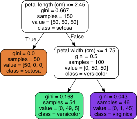
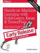
Figure 6-1. Iris Decision Tree

Making Predictions

Let’s see how the tree represented in Figure 6-1 makes predictions. Suppose you find an iris flower and you want to classify it. You start at the root node (depth 0, at the top): this node asks whether the flower’s petal length is smaller than 2.45 cm. If it is, then you move down to the root’s left child node (depth 1, left). In this case, it is a leaf node (i.e., it does not have any children nodes), so it does not ask any questions: you can simply look at the predicted class for that node and the Decision Tree predicts that your flower is an Iris-Setosa (class=setosa).

Now suppose you find another flower, but this time the petal length is greater than 2.45 cm. You must move down to the root’s right child node (depth 1, right), which is not a leaf node, so it asks another question: is the petal width smaller than 1.75 cm? If it is, then your flower is most likely an Iris-Versicolor (depth 2, left). If not, it is likely an Iris-Virginica (depth 2, right). It’s really that simple.

A node’s samples attribute counts how many training instances it applies to. For example, 100 training instances have a petal length greater than 2.45 cm (depth 1, right), among which 54 have a petal width smaller than 1.75 cm (depth 2, left). A node’s value attribute tells you how many training instances of each class this node applies to: for example, the bottom-right node applies to 0 Iris-Setosa, 1 Iris-Versicolor, and 45 Iris-Virginica. Finally, a node’s gini attribute measures its impurity: a node is “pure” (gini=0) if all training instances it applies to belong to the same class. For example, since the depth-1 left node applies only to Iris-Setosa training instances, it is pure and its gini score is 0. Equation 6-1 shows how the training algorithm computes the gini score G_i of the i^th node. For example, the depth-2 left node has a gini score equal to 1 – (0/54)² – (49/54)² – (5/54)² ≈ 0.168. Another impurity measure is discussed shortly.

• p_i,k is the ratio of class k instances among the training instances in the i^th node.

Figure 6-2 shows this Decision Tree’s decision boundaries. The thick vertical line represents the decision boundary of the root node (depth 0): petal length = 2.45 cm. Since the left area is pure (only Iris-Setosa), it cannot be split any further. However, the right area is impure, so the depth-1 right node splits it at petal width = 1.75 cm (represented by the dashed line). Since max_depth was set to 2, the Decision Tree stops right there. However, if you set max_depth to 3, then the two depth-2 nodes would each add another decision boundary (represented by the dotted lines).

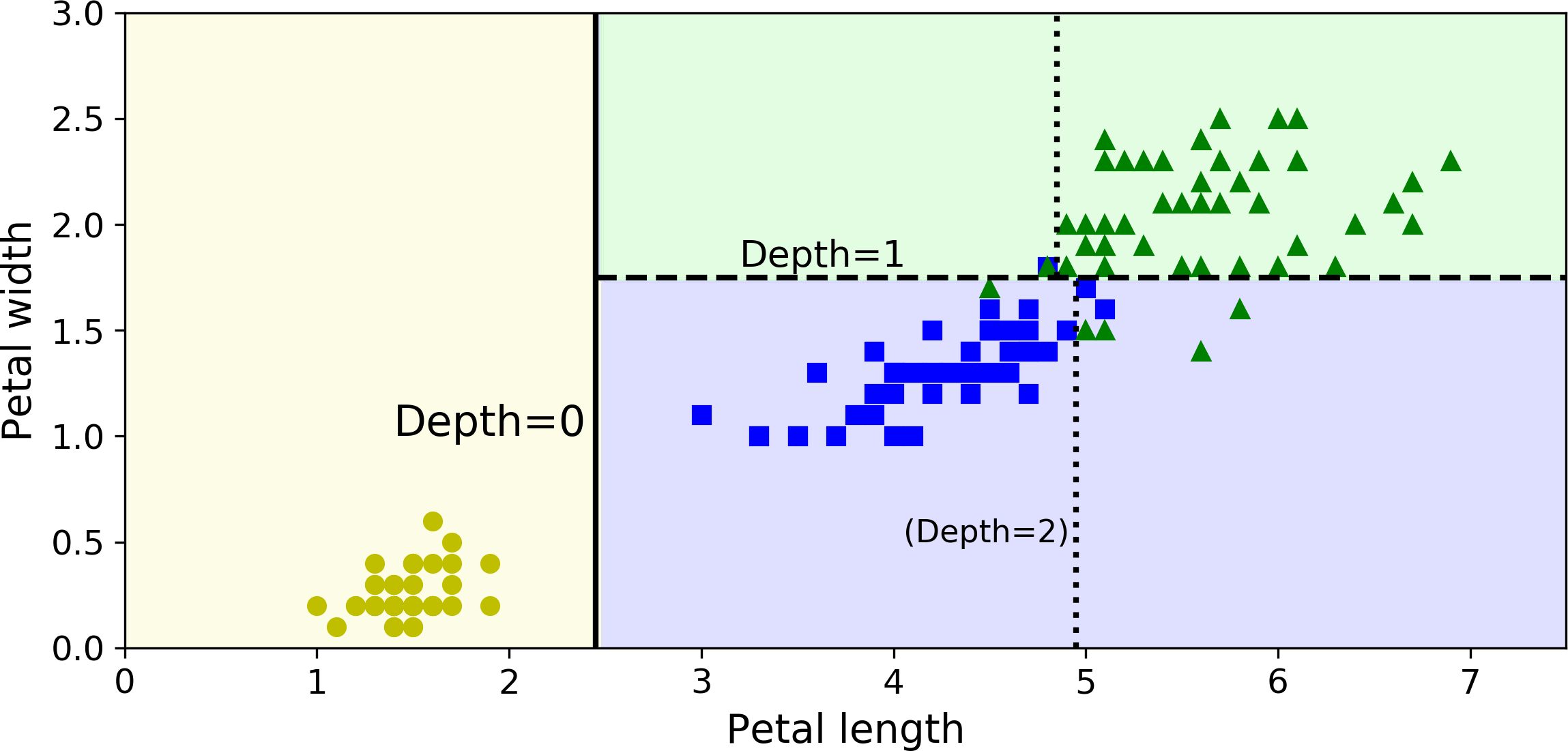
Figure 6-2. Decision Tree decision boundaries

Estimating Class Probabilities

A Decision Tree can also estimate the probability that an instance belongs to a particular class k: first it traverses the tree to find the leaf node for this instance, and then it returns the ratio of training instances of class k in this node. For example, suppose you have found a flower whose petals are 5 cm long and 1.5 cm wide. The corresponding leaf node is the depth-2 left node, so the Decision Tree should output the following probabilities: 0% for Iris-Setosa (0/54), 90.7% for Iris-Versicolor (49/54), and 9.3% for Iris-Virginica (5/54). And of course if you ask it to predict the class, it should output Iris-Versicolor (class 1) since it has the highest probability. Let’s check this:

>>> tree_clf.predict_proba([[5, 1.5]])
array([[0.        , 0.90740741, 0.09259259]])
>>> tree_clf.predict([[5, 1.5]])
array([1])

Perfect! Notice that the estimated probabilities would be identical anywhere else in the bottom-right rectangle of Figure 6-2—for example, if the petals were 6 cm long and 1.5 cm wide (even though it seems obvious that it would most likely be an Iris-Virginica in this case).

The CART Training Algorithm

Scikit-Learn uses the Classification And Regression Tree (CART) algorithm to train Decision Trees (also called “growing” trees). The idea is really quite simple: the algorithm first splits the training set in two subsets using a single feature k and a threshold t_k (e.g., “petal length ≤ 2.45 cm”). How does it choose k and t_k? It searches for the pair (k, t_k) that produces the purest subsets (weighted by their size). The cost function that the algorithm tries to minimize is given by Equation 6-2.

Once it has successfully split the training set in two, it splits the subsets using the same logic, then the sub-subsets and so on, recursively. It stops recursing once it reaches the maximum depth (defined by the max_depth hyperparameter), or if it cannot find a split that will reduce impurity. A few other hyperparameters (described in a moment) control additional stopping conditions (min_samples_split, min_samples_leaf, min_weight_fraction_leaf, and max_leaf_nodes).

Computational Complexity

Making predictions requires traversing the Decision Tree from the root to a leaf. Decision Trees are generally approximately balanced, so traversing the Decision Tree requires going through roughly O(log₂(m)) nodes.³ Since each node only requires checking the value of one feature, the overall prediction complexity is just O(log₂(m)), independent of the number of features. So predictions are very fast, even when dealing with large training sets.

However, the training algorithm compares all features (or less if max_features is set) on all samples at each node. This results in a training complexity of O(n × m log(m)). For small training sets (less than a few thousand instances), Scikit-Learn can speed up training by presorting the data (set presort=True), but this slows down training considerably for larger training sets.

Gini Impurity or Entropy?

By default, the Gini impurity measure is used, but you can select the entropy impurity measure instead by setting the criterion hyperparameter to "entropy". The concept of entropy originated in thermodynamics as a measure of molecular disorder: entropy approaches zero when molecules are still and well ordered. It later spread to a wide variety of domains, including Shannon’s information theory, where it measures the average information content of a message:⁴ entropy is zero when all messages are identical. In Machine Learning, it is frequently used as an impurity measure: a set’s entropy is zero when it contains instances of only one class. Equation 6-3 shows the definition of the entropy of the i^th node. For example, the depth-2 left node in Figure 6-1 has an entropy equal to $-\frac{49}{54}{log}_2\left(\frac{49}{54}\right)-\frac{5}{54}{log}_2\left(\frac{5}{54}\right)$ ≈ 0.445.

So should you use Gini impurity or entropy? The truth is, most of the time it does not make a big difference: they lead to similar trees. Gini impurity is slightly faster to compute, so it is a good default. However, when they differ, Gini impurity tends to isolate the most frequent class in its own branch of the tree, while entropy tends to produce slightly more balanced trees.⁵

Regularization Hyperparameters

Decision Trees make very few assumptions about the training data (as opposed to linear models, which obviously assume that the data is linear, for example). If left unconstrained, the tree structure will adapt itself to the training data, fitting it very closely, and most likely overfitting it. Such a model is often called a nonparametric model, not because it does not have any parameters (it often has a lot) but because the number of parameters is not determined prior to training, so the model structure is free to stick closely to the data. In contrast, a parametric model such as a linear model has a predetermined number of parameters, so its degree of freedom is limited, reducing the risk of overfitting (but increasing the risk of underfitting).

To avoid overfitting the training data, you need to restrict the Decision Tree’s freedom during training. As you know by now, this is called regularization. The regularization hyperparameters depend on the algorithm used, but generally you can at least restrict the maximum depth of the Decision Tree. In Scikit-Learn, this is controlled by the max_depth hyperparameter (the default value is None, which means unlimited). Reducing max_depth will regularize the model and thus reduce the risk of overfitting.

The DecisionTreeClassifier class has a few other parameters that similarly restrict the shape of the Decision Tree: min_samples_split (the minimum number of samples a node must have before it can be split), min_samples_leaf (the minimum number of samples a leaf node must have), min_weight_fraction_leaf (same as min_samples_leaf but expressed as a fraction of the total number of weighted instances), max_leaf_nodes (maximum number of leaf nodes), and max_features (maximum number of features that are evaluated for splitting at each node). Increasing min_* hyperparameters or reducing max_* hyperparameters will regularize the model.

Figure 6-3 shows two Decision Trees trained on the moons dataset (introduced in Chapter 5). On the left, the Decision Tree is trained with the default hyperparameters (i.e., no restrictions), and on the right the Decision Tree is trained with min_samples_leaf=4. It is quite obvious that the model on the left is overfitting, and the model on the right will probably generalize better.

Figure 6-3. Regularization using min_samples_leaf

Regression

Decision Trees are also capable of performing regression tasks. Let’s build a regression tree using Scikit-Learn’s DecisionTreeRegressor class, training it on a noisy quadratic dataset with max_depth=2:

from sklearn.tree import DecisionTreeRegressor

tree_reg = DecisionTreeRegressor(max_depth=2)
tree_reg.fit(X, y)

The resulting tree is represented on Figure 6-4.

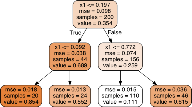
Figure 6-4. A Decision Tree for regression

This tree looks very similar to the classification tree you built earlier. The main difference is that instead of predicting a class in each node, it predicts a value. For example, suppose you want to make a prediction for a new instance with x₁ = 0.6. You traverse the tree starting at the root, and you eventually reach the leaf node that predicts value=0.1106. This prediction is simply the average target value of the 110 training instances associated to this leaf node. This prediction results in a Mean Squared Error (MSE) equal to 0.0151 over these 110 instances.

This model’s predictions are represented on the left of Figure 6-5. If you set max_depth=3, you get the predictions represented on the right. Notice how the predicted value for each region is always the average target value of the instances in that region. The algorithm splits each region in a way that makes most training instances as close as possible to that predicted value.

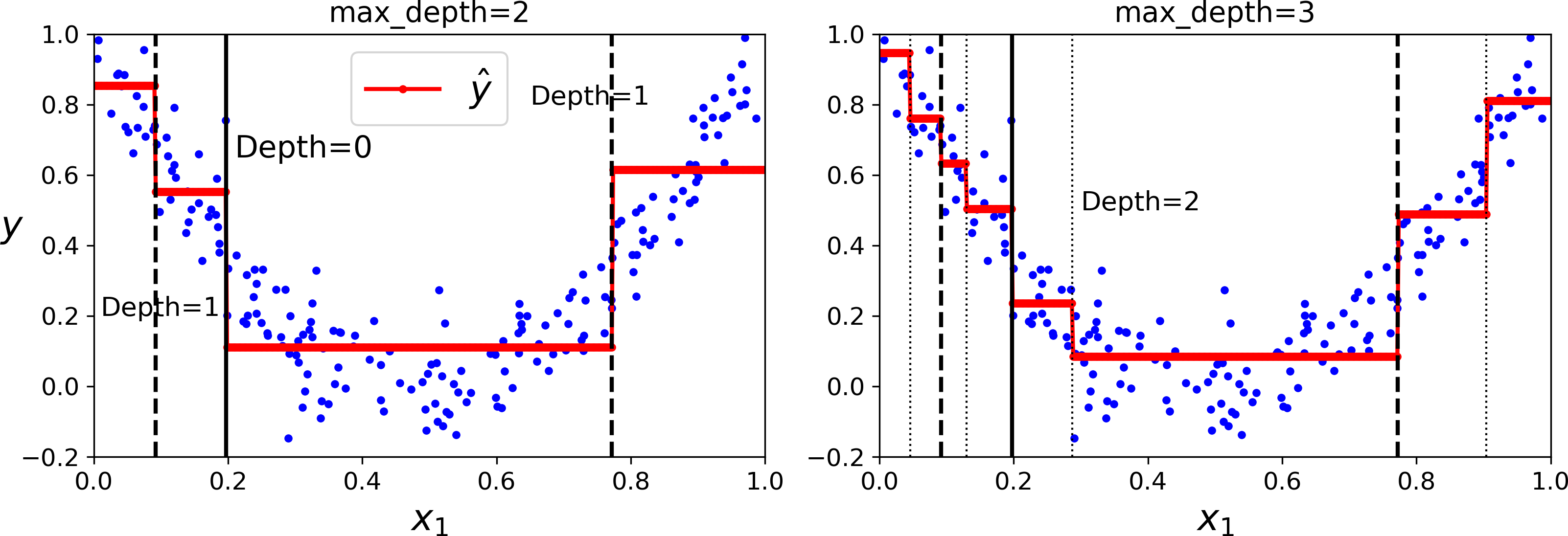
Figure 6-5. Predictions of two Decision Tree regression models

The CART algorithm works mostly the same way as earlier, except that instead of trying to split the training set in a way that minimizes impurity, it now tries to split the training set in a way that minimizes the MSE. Equation 6-4 shows the cost function that the algorithm tries to minimize.

Just like for classification tasks, Decision Trees are prone to overfitting when dealing with regression tasks. Without any regularization (i.e., using the default hyperparameters), you get the predictions on the left of Figure 6-6. It is obviously overfitting the training set very badly. Just setting min_samples_leaf=10 results in a much more reasonable model, represented on the right of Figure 6-6.

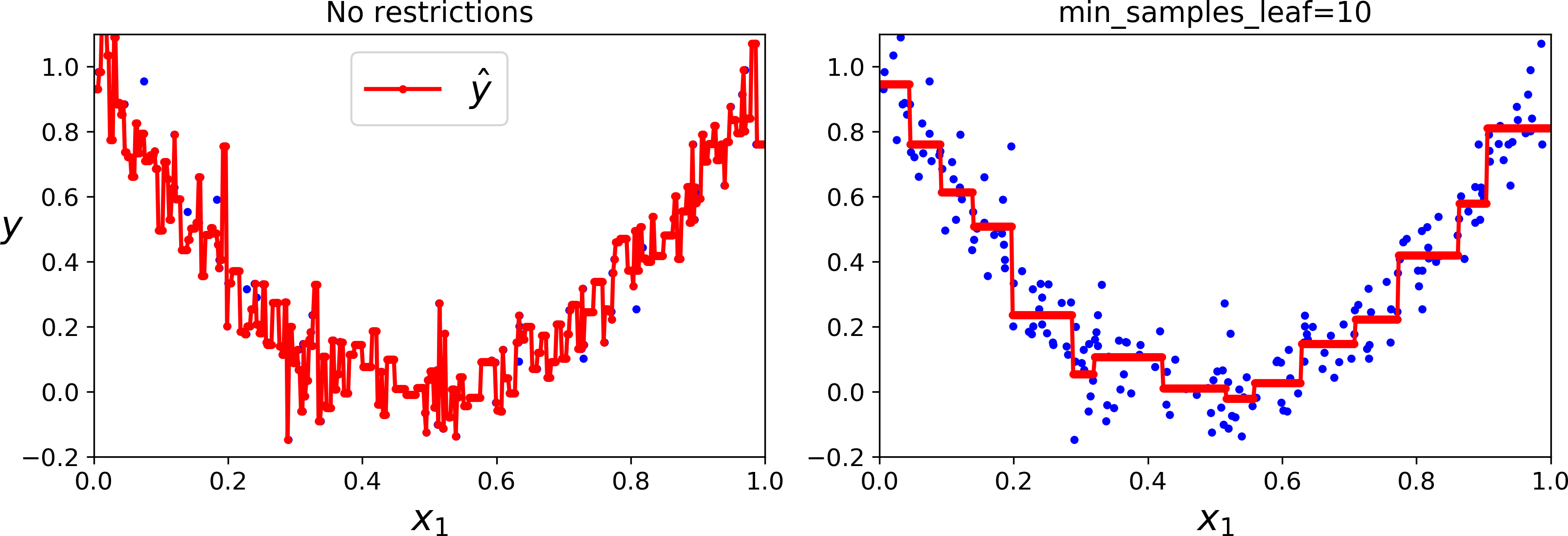
Figure 6-6. Regularizing a Decision Tree regressor

Instability

Hopefully by now you are convinced that Decision Trees have a lot going for them: they are simple to understand and interpret, easy to use, versatile, and powerful. However they do have a few limitations. First, as you may have noticed, Decision Trees love orthogonal decision boundaries (all splits are perpendicular to an axis), which makes them sensitive to training set rotation. For example, Figure 6-7 shows a simple linearly separable dataset: on the left, a Decision Tree can split it easily, while on the right, after the dataset is rotated by 45°, the decision boundary looks unnecessarily convoluted. Although both Decision Trees fit the training set perfectly, it is very likely that the model on the right will not generalize well. One way to limit this problem is to use PCA (see Chapter 8), which often results in a better orientation of the training data.

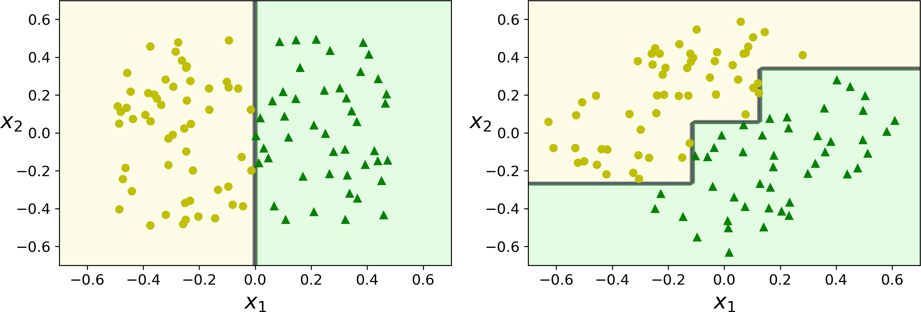
Figure 6-7. Sensitivity to training set rotation

More generally, the main issue with Decision Trees is that they are very sensitive to small variations in the training data. For example, if you just remove the widest Iris-Versicolor from the iris training set (the one with petals 4.8 cm long and 1.8 cm wide) and train a new Decision Tree, you may get the model represented in Figure 6-8. As you can see, it looks very different from the previous Decision Tree (Figure 6-2). Actually, since the training algorithm used by Scikit-Learn is stochastic⁶ you may get very different models even on the same training data (unless you set the random_state hyperparameter).

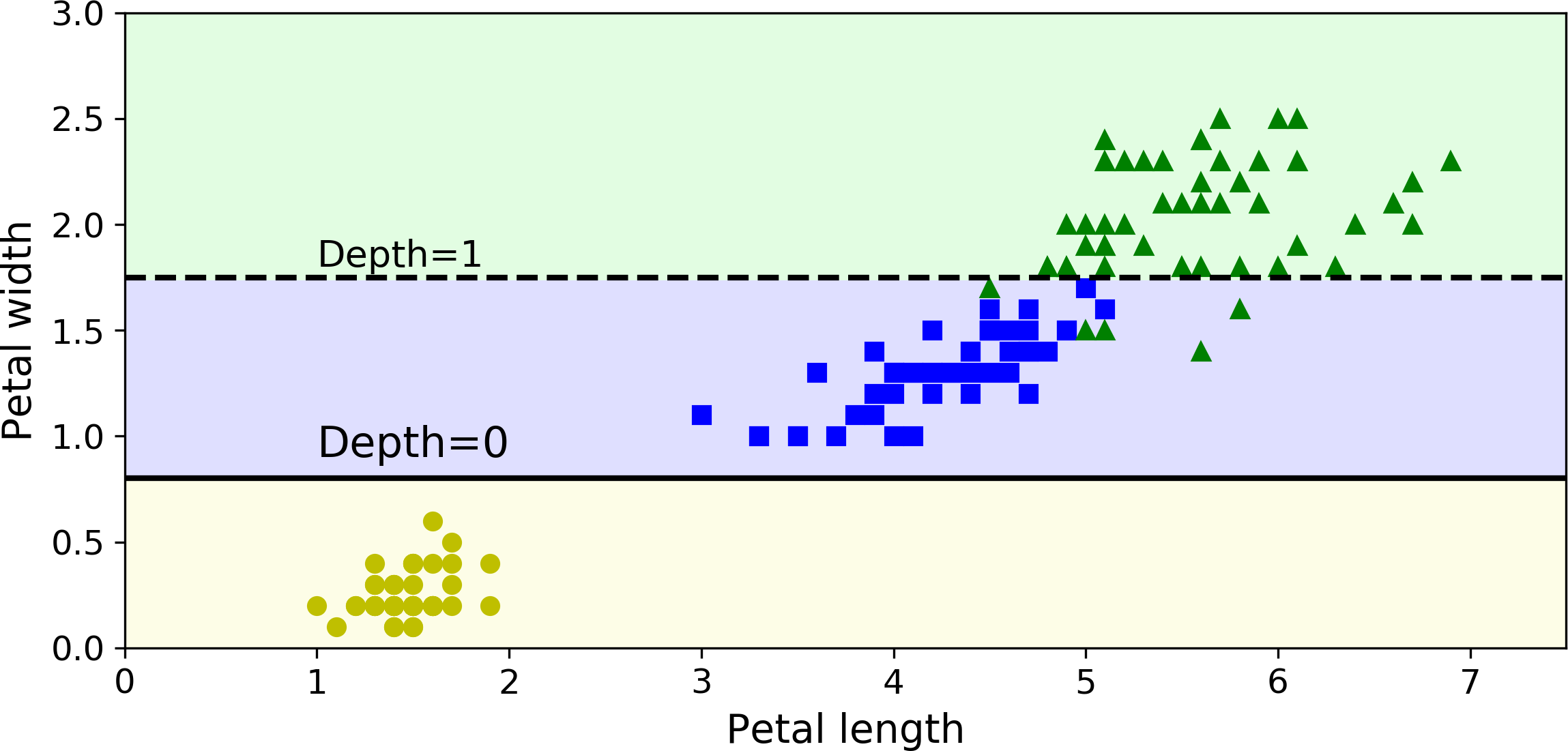
Figure 6-8. Sensitivity to training set details

Random Forests can limit this instability by averaging predictions over many trees, as we will see in the next chapter.

Exercises

1. What is the approximate depth of a Decision Tree trained (without restrictions) on a training set with 1 million instances?

2. Is a node’s Gini impurity generally lower or greater than its parent’s? Is it generally lower/greater, or always lower/greater?

3. If a Decision Tree is overfitting the training set, is it a good idea to try decreasing max_depth?

4. If a Decision Tree is underfitting the training set, is it a good idea to try scaling the input features?

5. If it takes one hour to train a Decision Tree on a training set containing 1 million instances, roughly how much time will it take to train another Decision Tree on a training set containing 10 million instances?

6. If your training set contains 100,000 instances, will setting presort=True speed up training?

7. Train and fine-tune a Decision Tree for the moons dataset.

   1. Generate a moons dataset using make_moons(n_samples=10000, noise=0.4).

   2. Split it into a training set and a test set using train_test_split().

   3. Use grid search with cross-validation (with the help of the GridSearchCV class) to find good hyperparameter values for a DecisionTreeClassifier. Hint: try various values for max_leaf_nodes.

   4. Train it on the full training set using these hyperparameters, and measure your model’s performance on the test set. You should get roughly 85% to 87% accuracy.

8. Grow a forest.

   1. Continuing the previous exercise, generate 1,000 subsets of the training set, each containing 100 instances selected randomly. Hint: you can use Scikit-Learn’s ShuffleSplit class for this.

   2. Train one Decision Tree on each subset, using the best hyperparameter values found above. Evaluate these 1,000 Decision Trees on the test set. Since they were trained on smaller sets, these Decision Trees will likely perform worse than the first Decision Tree, achieving only about 80% accuracy.

   3. Now comes the magic. For each test set instance, generate the predictions of the 1,000 Decision Trees, and keep only the most frequent prediction (you can use SciPy’s mode() function for this). This gives you majority-vote predictions over the test set.

   4. Evaluate these predictions on the test set: you should obtain a slightly higher accuracy than your first model (about 0.5 to 1.5% higher). Congratulations, you have trained a Random Forest classifier!

Solutions to these exercises are available in Appendix A.