Table of Contents for
Hands-on Machine Learning with Scikit-Learn, Keras, and TensorFlow, 2nd Edition
 Hands-on Machine Learning with Scikit-Learn, Keras, and TensorFlow, 2nd Edition
Published by
O'Reilly Media, Inc., 2019
Hands-on Machine Learning with Scikit-Learn, Keras, and TensorFlow, 2nd Edition
Published by
O'Reilly Media, Inc., 2019
- Cover
- nav
- Hands-on Machine Learning with Scikit-Learn, Keras, and TensorFlow
- Hands-on Machine Learning with Scikit-Learn, Keras, and TensorFlow
- 1. The Machine Learning Landscape
- 2. End-to-End Machine Learning Project
- 3. Classification
- 4. Training Models
- 5. Support Vector Machines
- 6. Decision Trees
- 7. Ensemble Learning and Random Forests
- 8. Dimensionality Reduction
- 9. Unsupervised Learning Techniques
- About the Author
- Colophon
Chapter 2. End-to-End Machine Learning Project
In this chapter, you will go through an example project end to end, pretending to be a recently hired data scientist in a real estate company.1 Here are the main steps you will go through:
-
Look at the big picture.
-
Get the data.
-
Discover and visualize the data to gain insights.
-
Prepare the data for Machine Learning algorithms.
-
Select a model and train it.
-
Fine-tune your model.
-
Present your solution.
-
Launch, monitor, and maintain your system.
Working with Real Data
When you are learning about Machine Learning it is best to actually experiment with real-world data, not just artificial datasets. Fortunately, there are thousands of open datasets to choose from, ranging across all sorts of domains. Here are a few places you can look to get data:
-
Popular open data repositories:
-
Meta portals (they list open data repositories):
-
Other pages listing many popular open data repositories:
In this chapter we chose the California Housing Prices dataset from the StatLib repository2 (see Figure 2-1). This dataset was based on data from the 1990 California census. It is not exactly recent (you could still afford a nice house in the Bay Area at the time), but it has many qualities for learning, so we will pretend it is recent data. We also added a categorical attribute and removed a few features for teaching purposes.
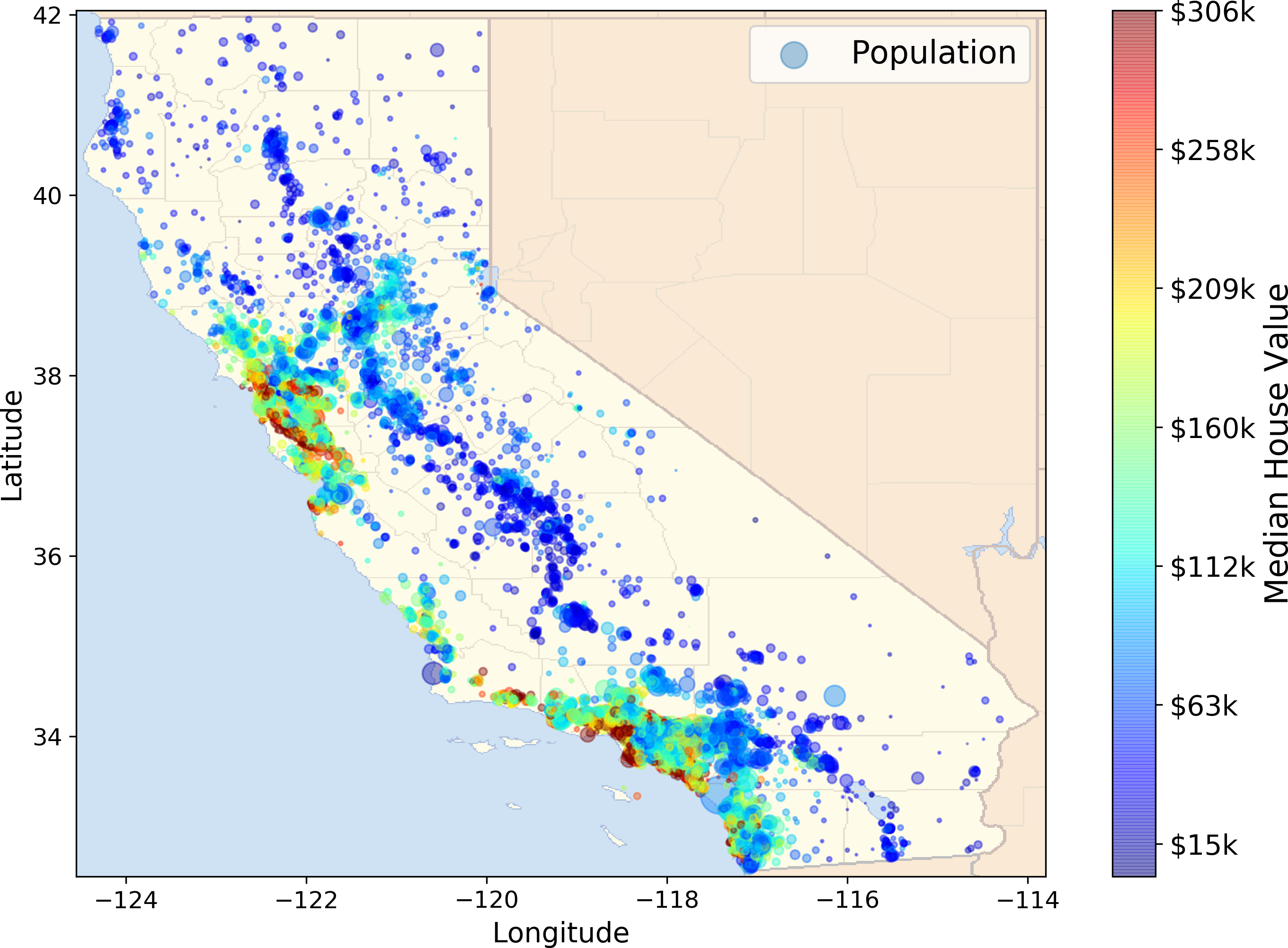
Figure 2-1. California housing prices
Look at the Big Picture
Welcome to Machine Learning Housing Corporation! The first task you are asked to perform is to build a model of housing prices in California using the California census data. This data has metrics such as the population, median income, median housing price, and so on for each block group in California. Block groups are the smallest geographical unit for which the US Census Bureau publishes sample data (a block group typically has a population of 600 to 3,000 people). We will just call them “districts” for short.
Your model should learn from this data and be able to predict the median housing price in any district, given all the other metrics.
Tip
Since you are a well-organized data scientist, the first thing you do is to pull out your Machine Learning project checklist. You can start with the one in Appendix B; it should work reasonably well for most Machine Learning projects but make sure to adapt it to your needs. In this chapter we will go through many checklist items, but we will also skip a few, either because they are self-explanatory or because they will be discussed in later chapters.
Frame the Problem
The first question to ask your boss is what exactly is the business objective; building a model is probably not the end goal. How does the company expect to use and benefit from this model? This is important because it will determine how you frame the problem, what algorithms you will select, what performance measure you will use to evaluate your model, and how much effort you should spend tweaking it.
Your boss answers that your model’s output (a prediction of a district’s median housing price) will be fed to another Machine Learning system (see Figure 2-2), along with many other signals.3 This downstream system will determine whether it is worth investing in a given area or not. Getting this right is critical, as it directly affects revenue.
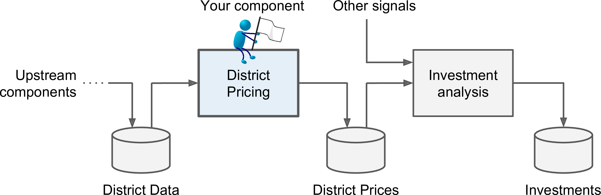
Figure 2-2. A Machine Learning pipeline for real estate investments
The next question to ask is what the current solution looks like (if any). It will often give you a reference performance, as well as insights on how to solve the problem. Your boss answers that the district housing prices are currently estimated manually by experts: a team gathers up-to-date information about a district, and when they cannot get the median housing price, they estimate it using complex rules.
This is costly and time-consuming, and their estimates are not great; in cases where they manage to find out the actual median housing price, they often realize that their estimates were off by more than 20%. This is why the company thinks that it would be useful to train a model to predict a district’s median housing price given other data about that district. The census data looks like a great dataset to exploit for this purpose, since it includes the median housing prices of thousands of districts, as well as other data.
Okay, with all this information you are now ready to start designing your system. First, you need to frame the problem: is it supervised, unsupervised, or Reinforcement Learning? Is it a classification task, a regression task, or something else? Should you use batch learning or online learning techniques? Before you read on, pause and try to answer these questions for yourself.
Have you found the answers? Let’s see: it is clearly a typical supervised learning task since you are given labeled training examples (each instance comes with the expected output, i.e., the district’s median housing price). Moreover, it is also a typical regression task, since you are asked to predict a value. More specifically, this is a multiple regression problem since the system will use multiple features to make a prediction (it will use the district’s population, the median income, etc.). It is also a univariate regression problem since we are only trying to predict a single value for each district. If we were trying to predict multiple values per district, it would be a multivariate regression problem. Finally, there is no continuous flow of data coming in the system, there is no particular need to adjust to changing data rapidly, and the data is small enough to fit in memory, so plain batch learning should do just fine.
Select a Performance Measure
Your next step is to select a performance measure. A typical performance measure for regression problems is the Root Mean Square Error (RMSE). It gives an idea of how much error the system typically makes in its predictions, with a higher weight for large errors. Equation 2-1 shows the mathematical formula to compute the RMSE.
Equation 2-1. Root Mean Square Error (RMSE)
Even though the RMSE is generally the preferred performance measure for regression tasks, in some contexts you may prefer to use another function. For example, suppose that there are many outlier districts. In that case, you may consider using the Mean Absolute Error (also called the Average Absolute Deviation; see Equation 2-2):
Equation 2-2. Mean Absolute Error
Both the RMSE and the MAE are ways to measure the distance between two vectors: the vector of predictions and the vector of target values. Various distance measures, or norms, are possible:
-
Computing the root of a sum of squares (RMSE) corresponds to the Euclidean norm: it is the notion of distance you are familiar with. It is also called the ℓ2 norm, noted ∥ · ∥2 (or just ∥ · ∥).
-
Computing the sum of absolutes (MAE) corresponds to the ℓ1 norm, noted ∥ · ∥1. It is sometimes called the Manhattan norm because it measures the distance between two points in a city if you can only travel along orthogonal city blocks.
-
More generally, the ℓk norm of a vector v containing n elements is defined as . ℓ0 just gives the number of non-zero elements in the vector, and ℓ∞ gives the maximum absolute value in the vector.
-
The higher the norm index, the more it focuses on large values and neglects small ones. This is why the RMSE is more sensitive to outliers than the MAE. But when outliers are exponentially rare (like in a bell-shaped curve), the RMSE performs very well and is generally preferred.
Check the Assumptions
Lastly, it is good practice to list and verify the assumptions that were made so far (by you or others); this can catch serious issues early on. For example, the district prices that your system outputs are going to be fed into a downstream Machine Learning system, and we assume that these prices are going to be used as such. But what if the downstream system actually converts the prices into categories (e.g., “cheap,” “medium,” or “expensive”) and then uses those categories instead of the prices themselves? In this case, getting the price perfectly right is not important at all; your system just needs to get the category right. If that’s so, then the problem should have been framed as a classification task, not a regression task. You don’t want to find this out after working on a regression system for months.
Fortunately, after talking with the team in charge of the downstream system, you are confident that they do indeed need the actual prices, not just categories. Great! You’re all set, the lights are green, and you can start coding now!
Get the Data
It’s time to get your hands dirty. Don’t hesitate to pick up your laptop and walk through the following code examples in a Jupyter notebook. The full Jupyter notebook is available at https://github.com/ageron/handson-ml2.
Create the Workspace
First you will need to have Python installed. It is probably already installed on your system. If not, you can get it at https://www.python.org/.5
Next you need to create a workspace directory for your Machine Learning code and datasets. Open a terminal and type the following commands (after the $ prompts):
$ export ML_PATH="$HOME/ml" # You can change the path if you prefer$ mkdir -p $ML_PATH
You will need a number of Python modules: Jupyter, NumPy, Pandas, Matplotlib, and Scikit-Learn. If you already have Jupyter running with all these modules installed, you can safely skip to “Download the Data”. If you don’t have them yet, there are many ways to install them (and their dependencies). You can use your system’s packaging system (e.g., apt-get on Ubuntu, or MacPorts or HomeBrew on macOS), install a Scientific Python distribution such as Anaconda and use its packaging system, or just use Python’s own packaging system, pip, which is included by default with the Python binary installers (since Python 2.7.9).6 You can check to see if pip is installed by typing the following command:
$ pip3 --versionpip 18.0 from [...]/lib/python3.6/site-packages (python 3.6)
You should make sure you have a recent version of pip installed. To upgrade the pip module, type:7
$ pip3 install --upgrade pipCollecting pip[...]Successfully installed pip-18.0
Now you can install all the required modules and their dependencies using this simple pip command (if you are not using a virtualenv, you will need administrator rights, or to add the --user option):
$ pip3 install --upgrade jupyter matplotlib numpy pandas scipy scikit-learnCollecting jupyterDownloading jupyter-1.0.0-py2.py3-none-any.whlCollecting matplotlib[...]
To check your installation, try to import every module like this:
$ python3 -c "import jupyter, matplotlib, numpy, pandas, scipy, sklearn"There should be no output and no error. Now you can fire up Jupyter by typing:
$ jupyter notebook[I 15:24 NotebookApp] Serving notebooks from local directory: [...]/ml[I 15:24 NotebookApp] 0 active kernels[I 15:24 NotebookApp] The Jupyter Notebook is running at: http://localhost:8888/[I 15:24 NotebookApp] Use Control-C to stop this server and shut down allkernels (twice to skip confirmation).
A Jupyter server is now running in your terminal, listening to port 8888. You can visit this server by opening your web browser to http://localhost:8888/ (this usually happens automatically when the server starts). You should see your empty workspace directory (containing only the env directory if you followed the preceding virtualenv instructions).
Now create a new Python notebook by clicking on the New button and selecting the appropriate Python version8 (see Figure 2-3).
This does three things: first, it creates a new notebook file called Untitled.ipynb in your workspace; second, it starts a Jupyter Python kernel to run this notebook; and third, it opens this notebook in a new tab. You should start by renaming this notebook to “Housing” (this will automatically rename the file to Housing.ipynb) by clicking Untitled and typing the new name.
Figure 2-3. Your workspace in Jupyter
A notebook contains a list of cells. Each cell can contain executable code or formatted text. Right now the notebook contains only one empty code cell, labeled “In [1]:”. Try typing print("Hello world!") in the cell, and click on the play button (see Figure 2-4) or press Shift-Enter. This sends the current cell to this notebook’s Python kernel, which runs it and returns the output. The result is displayed below the cell, and since we reached the end of the notebook, a new cell is automatically created. Go through the User Interface Tour from Jupyter’s Help menu to learn the basics.
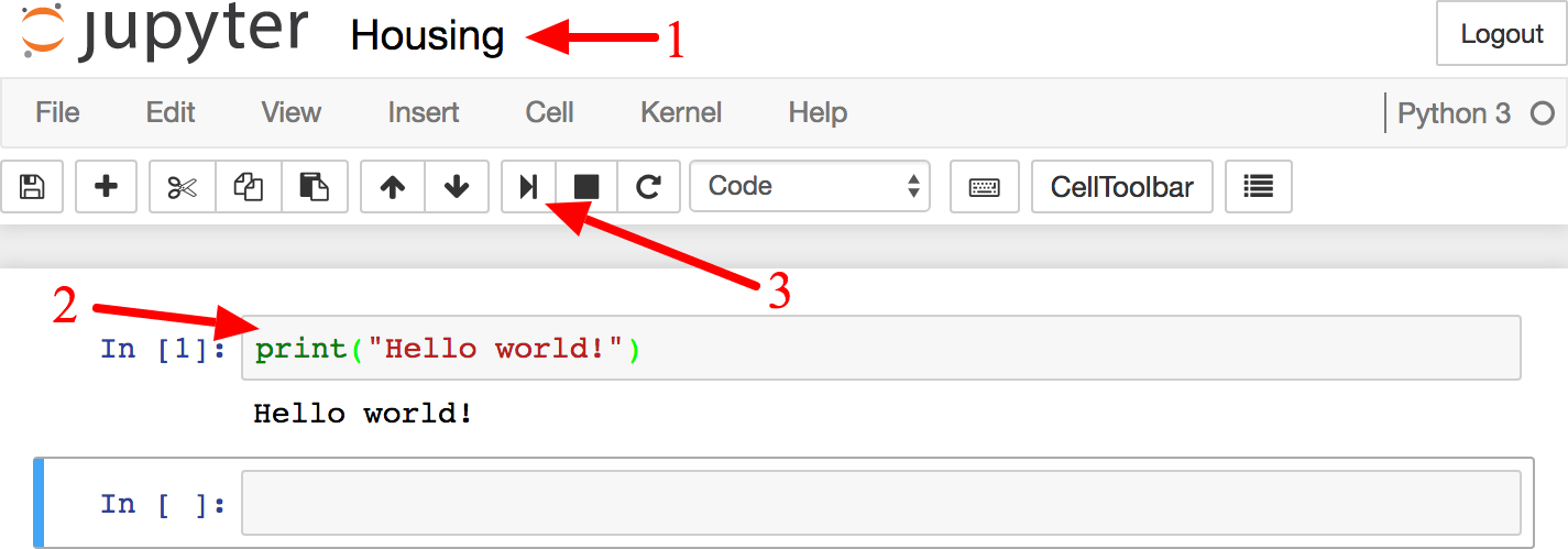
Figure 2-4. Hello world Python notebook
Download the Data
In typical environments your data would be available in a relational database (or some other common datastore) and spread across multiple tables/documents/files. To access it, you would first need to get your credentials and access authorizations,9 and familiarize yourself with the data schema. In this project, however, things are much simpler: you will just download a single compressed file, housing.tgz, which contains a comma-separated value (CSV) file called housing.csv with all the data.
You could use your web browser to download it, and run tar xzf housing.tgz to decompress the file and extract the CSV file, but it is preferable to create a small function to do that. It is useful in particular if data changes regularly, as it allows you to write a small script that you can run whenever you need to fetch the latest data (or you can set up a scheduled job to do that automatically at regular intervals). Automating the process of fetching the data is also useful if you need to install the dataset on multiple machines.
Here is the function to fetch the data:10
importosimporttarfilefromsix.movesimporturllibDOWNLOAD_ROOT="https://raw.githubusercontent.com/ageron/handson-ml2/master/"HOUSING_PATH=os.path.join("datasets","housing")HOUSING_URL=DOWNLOAD_ROOT+"datasets/housing/housing.tgz"deffetch_housing_data(housing_url=HOUSING_URL,housing_path=HOUSING_PATH):ifnotos.path.isdir(housing_path):os.makedirs(housing_path)tgz_path=os.path.join(housing_path,"housing.tgz")urllib.request.urlretrieve(housing_url,tgz_path)housing_tgz=tarfile.open(tgz_path)housing_tgz.extractall(path=housing_path)housing_tgz.close()
Now when you call fetch_housing_data(), it creates a datasets/housing directory in your workspace, downloads the housing.tgz file, and extracts the housing.csv from it in this directory.
Now let’s load the data using Pandas. Once again you should write a small function to load the data:
importpandasaspddefload_housing_data(housing_path=HOUSING_PATH):csv_path=os.path.join(housing_path,"housing.csv")returnpd.read_csv(csv_path)
This function returns a Pandas DataFrame object containing all the data.
Take a Quick Look at the Data Structure
Let’s take a look at the top five rows using the DataFrame’s head() method (see Figure 2-5).
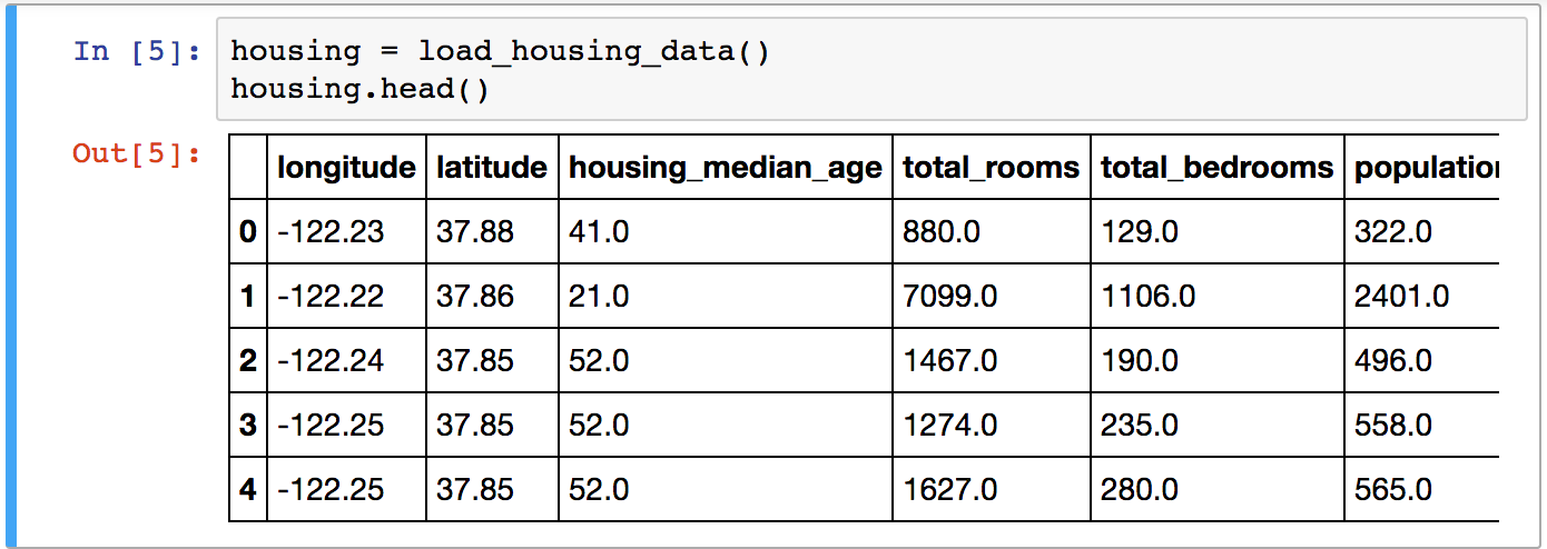
Figure 2-5. Top five rows in the dataset
Each row represents one district. There are 10 attributes (you can see the first 6 in the screenshot): longitude, latitude, housing_median_age, total_rooms, total_bedrooms, population, households, median_income, median_house_value, and ocean_proximity.
The info() method is useful to get a quick description of the data, in particular the total number of rows, and each attribute’s type and number of non-null values (see Figure 2-6).
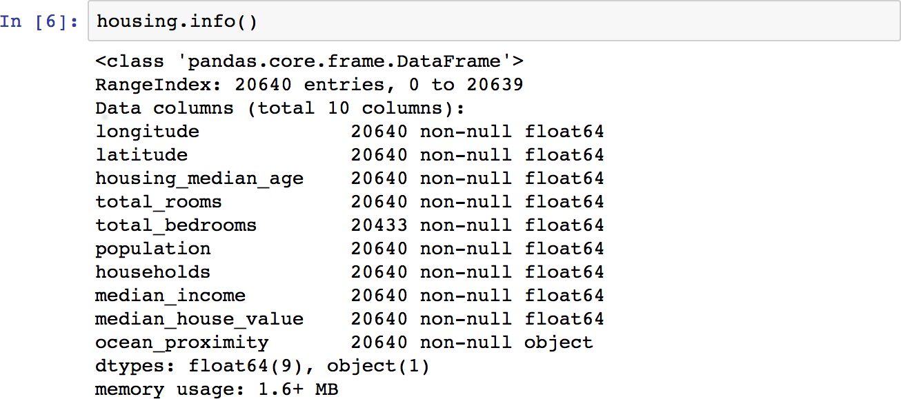
Figure 2-6. Housing info
There are 20,640 instances in the dataset, which means that it is fairly small by Machine Learning standards, but it’s perfect to get started. Notice that the total_bedrooms attribute has only 20,433 non-null values, meaning that 207 districts are missing this feature. We will need to take care of this later.
All attributes are numerical, except the ocean_proximity field. Its type is object, so it could hold any kind of Python object, but since you loaded this data from a CSV file you know that it must be a text attribute. When you looked at the top five rows, you probably noticed that the values in the ocean_proximity column were repetitive, which means that it is probably a categorical attribute. You can find out what categories exist and how many districts belong to each category by using the value_counts() method:
>>>housing["ocean_proximity"].value_counts()<1H OCEAN 9136INLAND 6551NEAR OCEAN 2658NEAR BAY 2290ISLAND 5Name: ocean_proximity, dtype: int64
Let’s look at the other fields. The describe() method shows a summary of the numerical attributes (Figure 2-7).
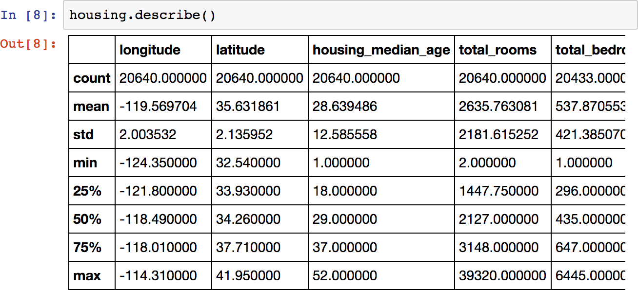
Figure 2-7. Summary of each numerical attribute
The count, mean, min, and max rows are self-explanatory. Note that the null values are ignored (so, for example, count of total_bedrooms is 20,433, not 20,640). The std row shows the standard deviation, which measures how dispersed the values are.11 The 25%, 50%, and 75% rows show the corresponding percentiles: a percentile indicates the value below which a given percentage of observations in a group of observations falls. For example, 25% of the districts have a housing_median_age lower than 18, while 50% are lower than 29 and 75% are lower than 37. These are often called the 25th percentile (or 1st quartile), the median, and the 75th percentile (or 3rd quartile).
Another quick way to get a feel of the type of data you are dealing with is to plot a histogram for each numerical attribute. A histogram shows the number of instances (on the vertical axis) that have a given value range (on the horizontal axis). You can either plot this one attribute at a time, or you can call the hist() method on the whole dataset, and it will plot a histogram for each numerical attribute (see Figure 2-8). For example, you can see that slightly over 800 districts have a median_house_value equal to about $100,000.
%matplotlibinline# only in a Jupyter notebookimportmatplotlib.pyplotasplthousing.hist(bins=50,figsize=(20,15))plt.show()
Note
The hist() method relies on Matplotlib, which in turn relies on a user-specified graphical backend to draw on your screen. So before you can plot anything, you need to specify which backend Matplotlib should use. The simplest option is to use Jupyter’s magic command %matplotlib inline. This tells Jupyter to set up Matplotlib so it uses Jupyter’s own backend. Plots are then rendered within the notebook itself. Note that calling show() is optional in a Jupyter notebook, as Jupyter will automatically display plots when a cell is executed.
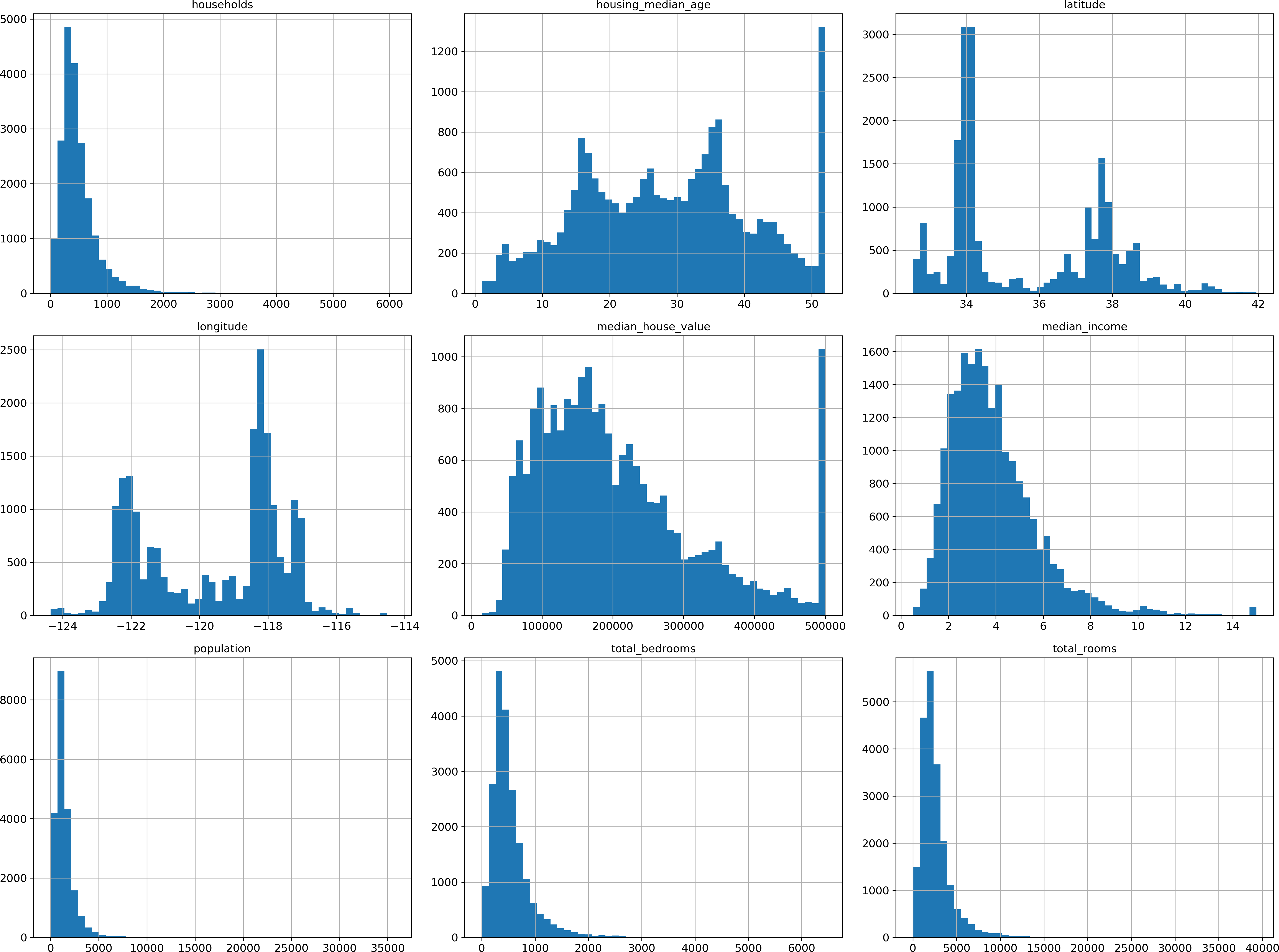
Figure 2-8. A histogram for each numerical attribute
Notice a few things in these histograms:
-
First, the median income attribute does not look like it is expressed in US dollars (USD). After checking with the team that collected the data, you are told that the data has been scaled and capped at 15 (actually 15.0001) for higher median incomes, and at 0.5 (actually 0.4999) for lower median incomes. The numbers represent roughly tens of thousands of dollars (e.g., 3 actually means about $30,000). Working with preprocessed attributes is common in Machine Learning, and it is not necessarily a problem, but you should try to understand how the data was computed.
-
The housing median age and the median house value were also capped. The latter may be a serious problem since it is your target attribute (your labels). Your Machine Learning algorithms may learn that prices never go beyond that limit. You need to check with your client team (the team that will use your system’s output) to see if this is a problem or not. If they tell you that they need precise predictions even beyond $500,000, then you have mainly two options:
-
Collect proper labels for the districts whose labels were capped.
-
Remove those districts from the training set (and also from the test set, since your system should not be evaluated poorly if it predicts values beyond $500,000).
-
-
These attributes have very different scales. We will discuss this later in this chapter when we explore feature scaling.
-
Finally, many histograms are tail heavy: they extend much farther to the right of the median than to the left. This may make it a bit harder for some Machine Learning algorithms to detect patterns. We will try transforming these attributes later on to have more bell-shaped distributions.
Hopefully you now have a better understanding of the kind of data you are dealing with.
Warning
Wait! Before you look at the data any further, you need to create a test set, put it aside, and never look at it.
Create a Test Set
It may sound strange to voluntarily set aside part of the data at this stage. After all, you have only taken a quick glance at the data, and surely you should learn a whole lot more about it before you decide what algorithms to use, right? This is true, but your brain is an amazing pattern detection system, which means that it is highly prone to overfitting: if you look at the test set, you may stumble upon some seemingly interesting pattern in the test data that leads you to select a particular kind of Machine Learning model. When you estimate the generalization error using the test set, your estimate will be too optimistic and you will launch a system that will not perform as well as expected. This is called data snooping bias.
Creating a test set is theoretically quite simple: just pick some instances randomly, typically 20% of the dataset, and set them aside:
importnumpyasnpdefsplit_train_test(data,test_ratio):shuffled_indices=np.random.permutation(len(data))test_set_size=int(len(data)*test_ratio)test_indices=shuffled_indices[:test_set_size]train_indices=shuffled_indices[test_set_size:]returndata.iloc[train_indices],data.iloc[test_indices]
You can then use this function like this:12
>>>train_set,test_set=split_train_test(housing,0.2)>>>len(train_set)16512>>>len(test_set)4128
Well, this works, but it is not perfect: if you run the program again, it will generate a different test set! Over time, you (or your Machine Learning algorithms) will get to see the whole dataset, which is what you want to avoid.
One solution is to save the test set on the first run and then load it in subsequent runs. Another option is to set the random number generator’s seed (e.g., np.random.seed(42))13 before calling np.random.permutation(), so that it always generates the same shuffled indices.
But both these solutions will break next time you fetch an updated dataset. A common solution is to use each instance’s identifier to decide whether or not it should go in the test set (assuming instances have a unique and immutable identifier). For example, you could compute a hash of each instance’s identifier and put that instance in the test set if the hash is lower or equal to 20% of the maximum hash value. This ensures that the test set will remain consistent across multiple runs, even if you refresh the dataset. The new test set will contain 20% of the new instances, but it will not contain any instance that was previously in the training set. Here is a possible implementation:
fromzlibimportcrc32deftest_set_check(identifier,test_ratio):returncrc32(np.int64(identifier))&0xffffffff<test_ratio*2**32defsplit_train_test_by_id(data,test_ratio,id_column):ids=data[id_column]in_test_set=ids.apply(lambdaid_:test_set_check(id_,test_ratio))returndata.loc[~in_test_set],data.loc[in_test_set]
Unfortunately, the housing dataset does not have an identifier column. The simplest solution is to use the row index as the ID:
housing_with_id=housing.reset_index()# adds an `index` columntrain_set,test_set=split_train_test_by_id(housing_with_id,0.2,"index")
If you use the row index as a unique identifier, you need to make sure that new data gets appended to the end of the dataset, and no row ever gets deleted. If this is not possible, then you can try to use the most stable features to build a unique identifier. For example, a district’s latitude and longitude are guaranteed to be stable for a few million years, so you could combine them into an ID like so:14
housing_with_id["id"]=housing["longitude"]*1000+housing["latitude"]train_set,test_set=split_train_test_by_id(housing_with_id,0.2,"id")
Scikit-Learn provides a few functions to split datasets into multiple subsets in various ways. The simplest function is train_test_split, which does pretty much the same thing as the function split_train_test defined earlier, with a couple of additional features. First there is a random_state parameter that allows you to set the random generator seed as explained previously, and second you can pass it multiple datasets with an identical number of rows, and it will split them on the same indices (this is very useful, for example, if you have a separate DataFrame for labels):
fromsklearn.model_selectionimporttrain_test_splittrain_set,test_set=train_test_split(housing,test_size=0.2,random_state=42)
So far we have considered purely random sampling methods. This is generally fine if your dataset is large enough (especially relative to the number of attributes), but if it is not, you run the risk of introducing a significant sampling bias. When a survey company decides to call 1,000 people to ask them a few questions, they don’t just pick 1,000 people randomly in a phone book. They try to ensure that these 1,000 people are representative of the whole population. For example, the US population is composed of 51.3% female and 48.7% male, so a well-conducted survey in the US would try to maintain this ratio in the sample: 513 female and 487 male. This is called stratified sampling: the population is divided into homogeneous subgroups called strata, and the right number of instances is sampled from each stratum to guarantee that the test set is representative of the overall population. If they used purely random sampling, there would be about 12% chance of sampling a skewed test set with either less than 49% female or more than 54% female. Either way, the survey results would be significantly biased.
Suppose you chatted with experts who told you that the median income is a very important attribute to predict median housing prices. You may want to ensure that the test set is representative of the various categories of incomes in the whole dataset. Since the median income is a continuous numerical attribute, you first need to create an income category attribute. Let’s look at the median income histogram more closely (back in Figure 2-8): most median income values are clustered around 2 to 5 (i.e., $20,000–$50,000), but some median incomes go far beyond 6 (i.e., $60,000). It is important to have a sufficient number of instances in your dataset for each stratum, or else the estimate of the stratum’s importance may be biased. This means that you should not have too many strata, and each stratum should be large enough. The following code creates an income category attribute by dividing the median income by 1.5 (to limit the number of income categories), and rounding up using ceil (to have discrete categories), and then keeping only the categories lower than 5 and merging the other categories into category 5:
housing["income_cat"]=np.ceil(housing["median_income"]/1.5)housing["income_cat"].where(housing["income_cat"]<5,5.0,inplace=True)
These income categories are represented in Figure 2-9:
housing["income_cat"].hist()
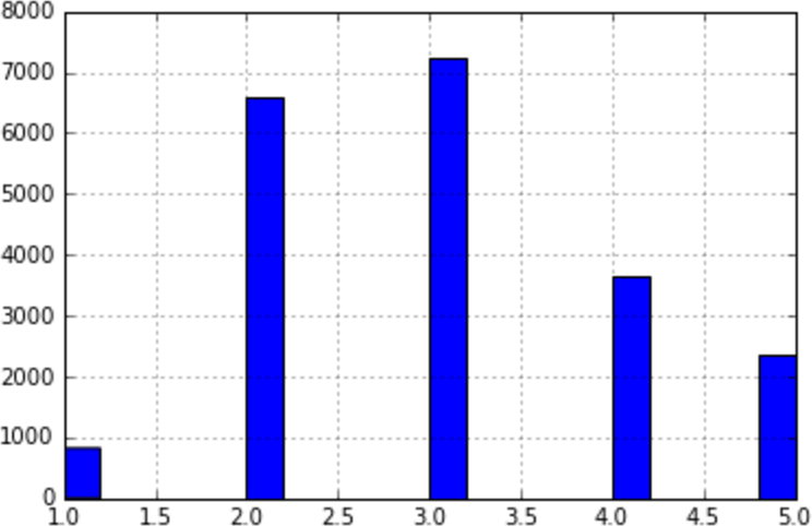
Figure 2-9. Histogram of income categories
Now you are ready to do stratified sampling based on the income category. For this you can use Scikit-Learn’s StratifiedShuffleSplit class:
fromsklearn.model_selectionimportStratifiedShuffleSplitsplit=StratifiedShuffleSplit(n_splits=1,test_size=0.2,random_state=42)fortrain_index,test_indexinsplit.split(housing,housing["income_cat"]):strat_train_set=housing.loc[train_index]strat_test_set=housing.loc[test_index]
Let’s see if this worked as expected. You can start by looking at the income category proportions in the test set:
>>>strat_test_set["income_cat"].value_counts()/len(strat_test_set)3.0 0.3505332.0 0.3187984.0 0.1763575.0 0.1145831.0 0.039729Name: income_cat, dtype: float64
With similar code you can measure the income category proportions in the full dataset. Figure 2-10 compares the income category proportions in the overall dataset, in the test set generated with stratified sampling, and in a test set generated using purely random sampling. As you can see, the test set generated using stratified sampling has income category proportions almost identical to those in the full dataset, whereas the test set generated using purely random sampling is quite skewed.
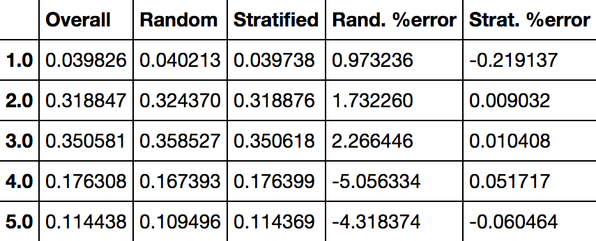
Figure 2-10. Sampling bias comparison of stratified versus purely random sampling
Now you should remove the income_cat attribute so the data is back to its original state:
forset_in(strat_train_set,strat_test_set):set_.drop("income_cat",axis=1,inplace=True)
We spent quite a bit of time on test set generation for a good reason: this is an often neglected but critical part of a Machine Learning project. Moreover, many of these ideas will be useful later when we discuss cross-validation. Now it’s time to move on to the next stage: exploring the data.
Discover and Visualize the Data to Gain Insights
So far you have only taken a quick glance at the data to get a general understanding of the kind of data you are manipulating. Now the goal is to go a little bit more in depth.
First, make sure you have put the test set aside and you are only exploring the training set. Also, if the training set is very large, you may want to sample an exploration set, to make manipulations easy and fast. In our case, the set is quite small so you can just work directly on the full set. Let’s create a copy so you can play with it without harming the training set:
housing=strat_train_set.copy()
Visualizing Geographical Data
Since there is geographical information (latitude and longitude), it is a good idea to create a scatterplot of all districts to visualize the data (Figure 2-11):
housing.plot(kind="scatter",x="longitude",y="latitude")
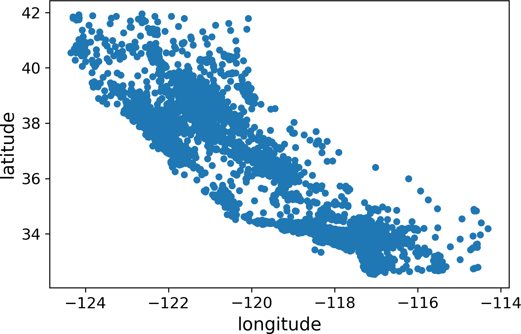
Figure 2-11. A geographical scatterplot of the data
This looks like California all right, but other than that it is hard to see any particular pattern. Setting the alpha option to 0.1 makes it much easier to visualize the places where there is a high density of data points (Figure 2-12):
housing.plot(kind="scatter",x="longitude",y="latitude",alpha=0.1)
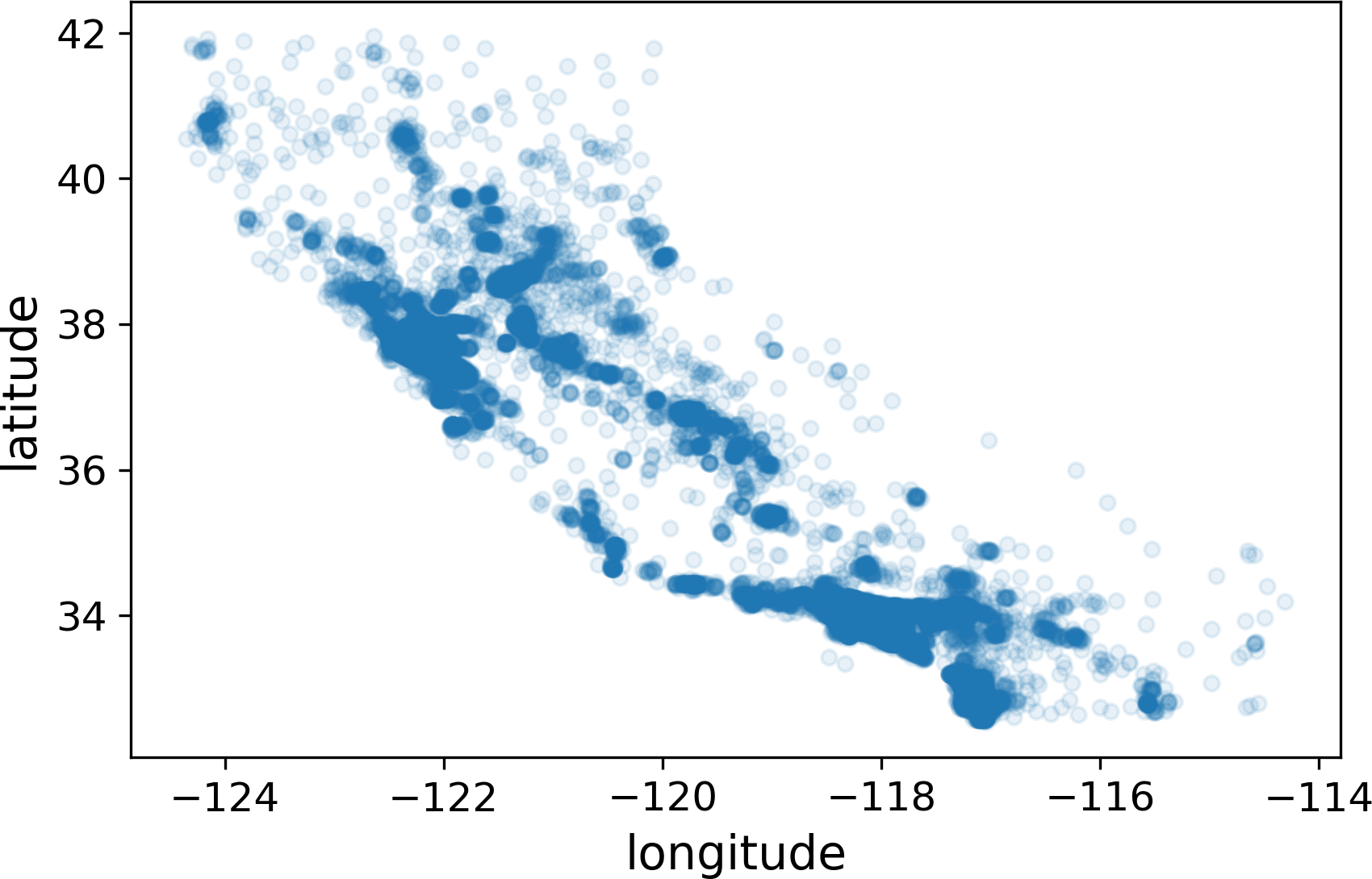
Figure 2-12. A better visualization highlighting high-density areas
Now that’s much better: you can clearly see the high-density areas, namely the Bay Area and around Los Angeles and San Diego, plus a long line of fairly high density in the Central Valley, in particular around Sacramento and Fresno.
More generally, our brains are very good at spotting patterns on pictures, but you may need to play around with visualization parameters to make the patterns stand out.
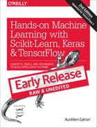
Now let’s look at the housing prices (Figure 2-13). The radius of each circle represents the district’s population (option s), and the color represents the price (option c). We will use a predefined color map (option cmap) called jet, which ranges from blue (low values) to red (high prices):15
housing.plot(kind="scatter",x="longitude",y="latitude",alpha=0.4,s=housing["population"]/100,label="population",figsize=(10,7),c="median_house_value",cmap=plt.get_cmap("jet"),colorbar=True,)plt.legend()
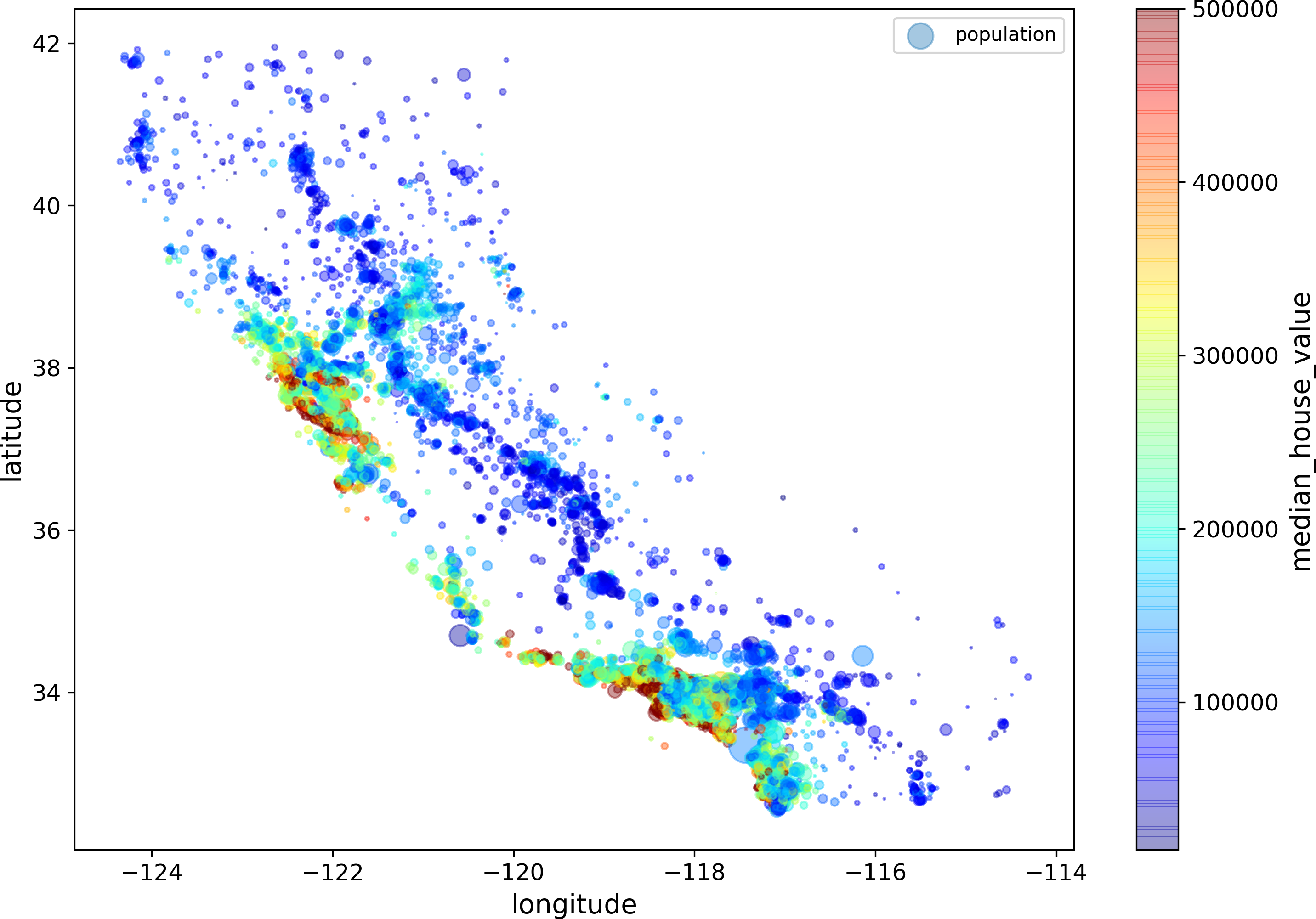
Figure 2-13. California housing prices
This image tells you that the housing prices are very much related to the location (e.g., close to the ocean) and to the population density, as you probably knew already. It will probably be useful to use a clustering algorithm to detect the main clusters, and add new features that measure the proximity to the cluster centers. The ocean proximity attribute may be useful as well, although in Northern California the housing prices in coastal districts are not too high, so it is not a simple rule.
Looking for Correlations
Since the dataset is not too large, you can easily compute the standard correlation coefficient (also called Pearson’s r) between every pair of attributes using the corr() method:
corr_matrix=housing.corr()
Now let’s look at how much each attribute correlates with the median house value:
>>>corr_matrix["median_house_value"].sort_values(ascending=False)median_house_value 1.000000median_income 0.687170total_rooms 0.135231housing_median_age 0.114220households 0.064702total_bedrooms 0.047865population -0.026699longitude -0.047279latitude -0.142826Name: median_house_value, dtype: float64
The correlation coefficient ranges from –1 to 1. When it is close to 1, it means that there is a strong positive correlation; for example, the median house value tends to go up when the median income goes up. When the coefficient is close to –1, it means that there is a strong negative correlation; you can see a small negative correlation between the latitude and the median house value (i.e., prices have a slight tendency to go down when you go north). Finally, coefficients close to zero mean that there is no linear correlation. Figure 2-14 shows various plots along with the correlation coefficient between their horizontal and vertical axes.
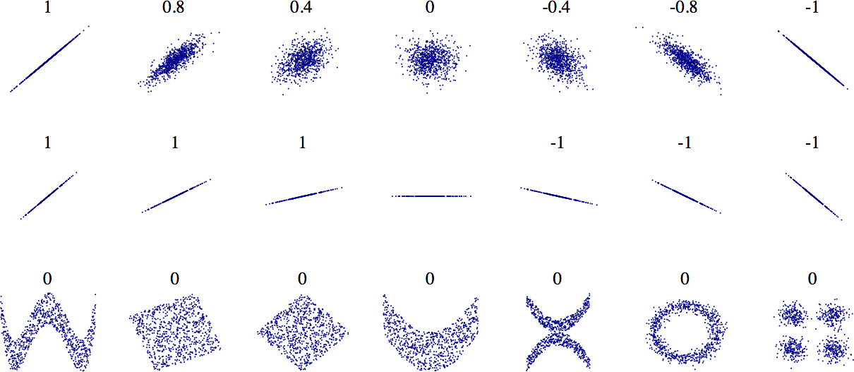
Figure 2-14. Standard correlation coefficient of various datasets (source: Wikipedia; public domain image)
Warning
The correlation coefficient only measures linear correlations (“if x goes up, then y generally goes up/down”). It may completely miss out on nonlinear relationships (e.g., “if x is close to zero then y generally goes up”). Note how all the plots of the bottom row have a correlation coefficient equal to zero despite the fact that their axes are clearly not independent: these are examples of nonlinear relationships. Also, the second row shows examples where the correlation coefficient is equal to 1 or –1; notice that this has nothing to do with the slope. For example, your height in inches has a correlation coefficient of 1 with your height in feet or in nanometers.
Another way to check for correlation between attributes is to use Pandas’ scatter_matrix function, which plots every numerical attribute against every other numerical attribute. Since there are now 11 numerical attributes, you would get 112 = 121 plots, which would not fit on a page, so let’s just focus on a few promising attributes that seem most correlated with the median housing value (Figure 2-15):
frompandas.plottingimportscatter_matrixattributes=["median_house_value","median_income","total_rooms","housing_median_age"]scatter_matrix(housing[attributes],figsize=(12,8))
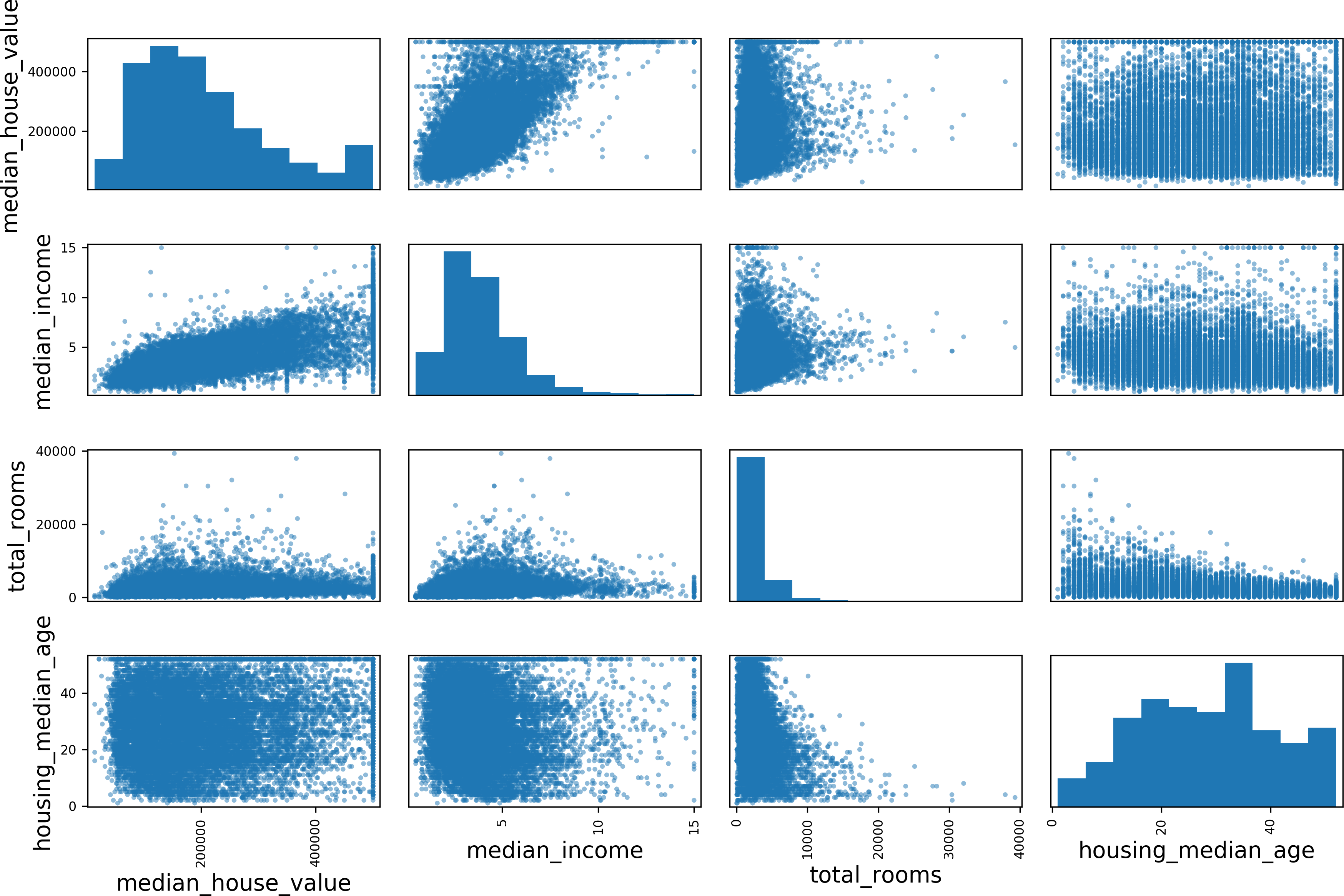
Figure 2-15. Scatter matrix
The main diagonal (top left to bottom right) would be full of straight lines if Pandas plotted each variable against itself, which would not be very useful. So instead Pandas displays a histogram of each attribute (other options are available; see Pandas’ documentation for more details).
The most promising attribute to predict the median house value is the median income, so let’s zoom in on their correlation scatterplot (Figure 2-16):
housing.plot(kind="scatter",x="median_income",y="median_house_value",alpha=0.1)
This plot reveals a few things. First, the correlation is indeed very strong; you can clearly see the upward trend and the points are not too dispersed. Second, the price cap that we noticed earlier is clearly visible as a horizontal line at $500,000. But this plot reveals other less obvious straight lines: a horizontal line around $450,000, another around $350,000, perhaps one around $280,000, and a few more below that. You may want to try removing the corresponding districts to prevent your algorithms from learning to reproduce these data quirks.
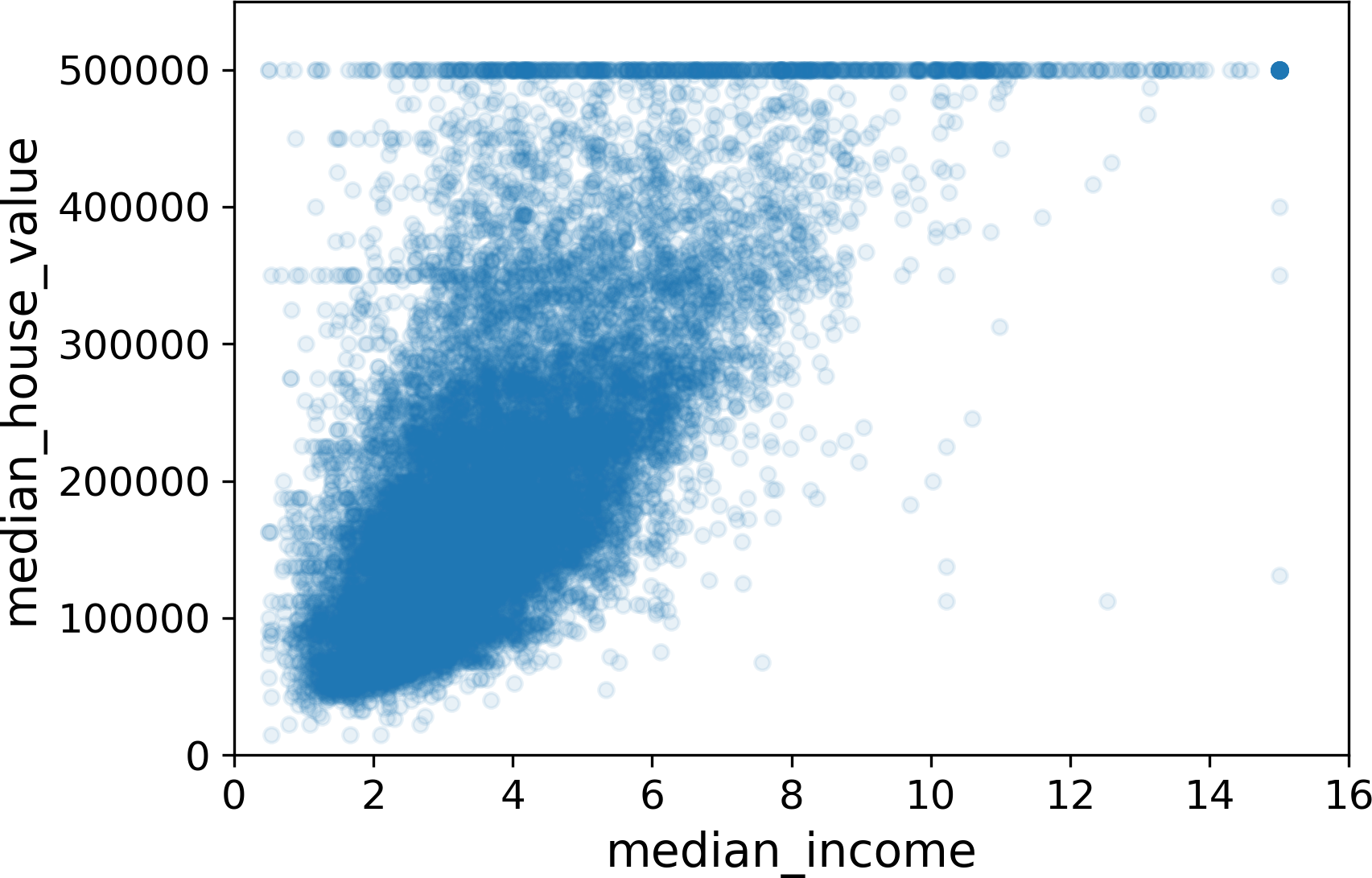
Figure 2-16. Median income versus median house value
Experimenting with Attribute Combinations
Hopefully the previous sections gave you an idea of a few ways you can explore the data and gain insights. You identified a few data quirks that you may want to clean up before feeding the data to a Machine Learning algorithm, and you found interesting correlations between attributes, in particular with the target attribute. You also noticed that some attributes have a tail-heavy distribution, so you may want to transform them (e.g., by computing their logarithm). Of course, your mileage will vary considerably with each project, but the general ideas are similar.
One last thing you may want to do before actually preparing the data for Machine Learning algorithms is to try out various attribute combinations. For example, the total number of rooms in a district is not very useful if you don’t know how many households there are. What you really want is the number of rooms per household. Similarly, the total number of bedrooms by itself is not very useful: you probably want to compare it to the number of rooms. And the population per household also seems like an interesting attribute combination to look at. Let’s create these new attributes:
housing["rooms_per_household"]=housing["total_rooms"]/housing["households"]housing["bedrooms_per_room"]=housing["total_bedrooms"]/housing["total_rooms"]housing["population_per_household"]=housing["population"]/housing["households"]
And now let’s look at the correlation matrix again:
>>>corr_matrix=housing.corr()>>>corr_matrix["median_house_value"].sort_values(ascending=False)median_house_value 1.000000median_income 0.687160rooms_per_household 0.146285total_rooms 0.135097housing_median_age 0.114110households 0.064506total_bedrooms 0.047689population_per_household -0.021985population -0.026920longitude -0.047432latitude -0.142724bedrooms_per_room -0.259984Name: median_house_value, dtype: float64
Hey, not bad! The new bedrooms_per_room attribute is much more correlated with the median house value than the total number of rooms or bedrooms. Apparently houses with a lower bedroom/room ratio tend to be more expensive. The number of rooms per household is also more informative than the total number of rooms in a district—obviously the larger the houses, the more expensive they are.
This round of exploration does not have to be absolutely thorough; the point is to start off on the right foot and quickly gain insights that will help you get a first reasonably good prototype. But this is an iterative process: once you get a prototype up and running, you can analyze its output to gain more insights and come back to this exploration step.
Prepare the Data for Machine Learning Algorithms
It’s time to prepare the data for your Machine Learning algorithms. Instead of just doing this manually, you should write functions to do that, for several good reasons:
-
This will allow you to reproduce these transformations easily on any dataset (e.g., the next time you get a fresh dataset).
-
You will gradually build a library of transformation functions that you can reuse in future projects.
-
You can use these functions in your live system to transform the new data before feeding it to your algorithms.
-
This will make it possible for you to easily try various transformations and see which combination of transformations works best.
But first let’s revert to a clean training set (by copying strat_train_set once again), and let’s separate the predictors and the labels since we don’t necessarily want to apply the same transformations to the predictors and the target values (note that drop() creates a copy of the data and does not affect strat_train_set):
housing=strat_train_set.drop("median_house_value",axis=1)housing_labels=strat_train_set["median_house_value"].copy()
Data Cleaning
Most Machine Learning algorithms cannot work with missing features, so let’s create a few functions to take care of them. You noticed earlier that the total_bedrooms attribute has some missing values, so let’s fix this. You have three options:
-
Get rid of the corresponding districts.
-
Get rid of the whole attribute.
-
Set the values to some value (zero, the mean, the median, etc.).
You can accomplish these easily using DataFrame’s dropna(), drop(), and fillna() methods:
housing.dropna(subset=["total_bedrooms"])# option 1housing.drop("total_bedrooms",axis=1)# option 2median=housing["total_bedrooms"].median()# option 3housing["total_bedrooms"].fillna(median,inplace=True)
If you choose option 3, you should compute the median value on the training set, and use it to fill the missing values in the training set, but also don’t forget to save the median value that you have computed. You will need it later to replace missing values in the test set when you want to evaluate your system, and also once the system goes live to replace missing values in new data.
Scikit-Learn provides a handy class to take care of missing values: SimpleImputer. Here is how to use it. First, you need to create a SimpleImputer instance, specifying that you want to replace each attribute’s missing values with the median of that attribute:
fromsklearn.imputeimportSimpleImputerimputer=SimpleImputer(strategy="median")
Since the median can only be computed on numerical attributes, we need to create a copy of the data without the text attribute ocean_proximity:
housing_num=housing.drop("ocean_proximity",axis=1)
Now you can fit the imputer instance to the training data using the fit() method:
imputer.fit(housing_num)
The imputer has simply computed the median of each attribute and stored the result in its statistics_ instance variable. Only the total_bedrooms attribute had missing values, but we cannot be sure that there won’t be any missing values in new data after the system goes live, so it is safer to apply the imputer to all the numerical attributes:
>>>imputer.statistics_array([ -118.51 , 34.26 , 29. , 2119.5 , 433. , 1164. , 408. , 3.5409])>>>housing_num.median().valuesarray([ -118.51 , 34.26 , 29. , 2119.5 , 433. , 1164. , 408. , 3.5409])
Now you can use this “trained” imputer to transform the training set by replacing missing values by the learned medians:
X=imputer.transform(housing_num)
The result is a plain NumPy array containing the transformed features. If you want to put it back into a Pandas DataFrame, it’s simple:
housing_tr=pd.DataFrame(X,columns=housing_num.columns)
Handling Text and Categorical Attributes
Earlier we left out the categorical attribute ocean_proximity because it is a text attribute so we cannot compute its median:
>>>housing_cat=housing[["ocean_proximity"]]>>>housing_cat.head(10)ocean_proximity17606 <1H OCEAN18632 <1H OCEAN14650 NEAR OCEAN3230 INLAND3555 <1H OCEAN19480 INLAND8879 <1H OCEAN13685 INLAND4937 <1H OCEAN4861 <1H OCEAN
Most Machine Learning algorithms prefer to work with numbers anyway, so let’s convert these categories from text to numbers. For this, we can use Scikit-Learn’s OrdinalEncoder class18:
>>>fromsklearn.preprocessingimportOrdinalEncoder>>>ordinal_encoder=OrdinalEncoder()>>>housing_cat_encoded=ordinal_encoder.fit_transform(housing_cat)>>>housing_cat_encoded[:10]array([[0.],[0.],[4.],[1.],[0.],[1.],[0.],[1.],[0.],[0.]])
You can get the list of categories using the categories_ instance variable. It is a list containing a 1D array of categories for each categorical attribute (in this case, a list containing a single array since there is just one categorical attribute):
>>>ordinal_encoder.categories_[array(['<1H OCEAN', 'INLAND', 'ISLAND', 'NEAR BAY', 'NEAR OCEAN'],dtype=object)]
One issue with this representation is that ML algorithms will assume that two nearby values are more similar than two distant values. This may be fine in some cases (e.g., for ordered categories such as “bad”, “average”, “good”, “excellent”), but it is obviously not the case for the ocean_proximity column (for example, categories 0 and 4 are clearly more similar than categories 0 and 1). To fix this issue, a common solution is to create one binary attribute per category: one attribute equal to 1 when the category is “<1H OCEAN” (and 0 otherwise), another attribute equal to 1 when the category is “INLAND” (and 0 otherwise), and so on. This is called one-hot encoding, because only one attribute will be equal to 1 (hot), while the others will be 0 (cold). The new attributes are sometimes called dummy attributes. Scikit-Learn provides a OneHotEncoder class to convert categorical values into one-hot vectors19:
>>>fromsklearn.preprocessingimportOneHotEncoder>>>cat_encoder=OneHotEncoder()>>>housing_cat_1hot=cat_encoder.fit_transform(housing_cat)>>>housing_cat_1hot<16512x5 sparse matrix of type '<class 'numpy.float64'>'with 16512 stored elements in Compressed Sparse Row format>
Notice that the output is a SciPy sparse matrix, instead of a NumPy array. This is very useful when you have categorical attributes with thousands of categories. After one-hot encoding we get a matrix with thousands of columns, and the matrix is full of zeros except for a single 1 per row. Using up tons of memory mostly to store zeros would be very wasteful, so instead a sparse matrix only stores the location of the nonzero elements. You can use it mostly like a normal 2D array,20 but if you really want to convert it to a (dense) NumPy array, just call the toarray() method:
>>>housing_cat_1hot.toarray()array([[1., 0., 0., 0., 0.],[1., 0., 0., 0., 0.],[0., 0., 0., 0., 1.],...,[0., 1., 0., 0., 0.],[1., 0., 0., 0., 0.],[0., 0., 0., 1., 0.]])
Once again, you can get the list of categories using the encoder’s categories_ instance variable:
>>>cat_encoder.categories_[array(['<1H OCEAN', 'INLAND', 'ISLAND', 'NEAR BAY', 'NEAR OCEAN'],dtype=object)]
Tip
If a categorical attribute has a large number of possible categories (e.g., country code, profession, species, etc.), then one-hot encoding will result in a large number of input features. This may slow down training and degrade performance. If this happens, you may want to replace the categorical input with useful numerical features related to the categories: for example, you could replace the ocean_proximity feature with the distance to the ocean (similarly, a country code could be replaced with the country’s population and GDP per capita). Alternatively, you could replace each category with a learnable low dimensional vector called an embedding. Each category’s representation would be learned during training: this is called representation learning (see Chapter 15 for more details).
Custom Transformers
Although Scikit-Learn provides many useful transformers, you will need to write your own for tasks such as custom cleanup operations or combining specific attributes. You will want your transformer to work seamlessly with Scikit-Learn functionalities (such as pipelines), and since Scikit-Learn relies on duck typing (not inheritance), all you need is to create a class and implement three methods: fit() (returning self), transform(), and fit_transform(). You can get the last one for free by simply adding TransformerMixin as a base class. Also, if you add BaseEstimator as a base class (and avoid *args and **kargs in your constructor) you will get two extra methods (get_params() and set_params()) that will be useful for automatic hyperparameter tuning. For example, here is a small transformer class that adds the combined attributes we discussed earlier:
fromsklearn.baseimportBaseEstimator,TransformerMixinrooms_ix,bedrooms_ix,population_ix,households_ix=3,4,5,6classCombinedAttributesAdder(BaseEstimator,TransformerMixin):def__init__(self,add_bedrooms_per_room=True):# no *args or **kargsself.add_bedrooms_per_room=add_bedrooms_per_roomdeffit(self,X,y=None):returnself# nothing else to dodeftransform(self,X,y=None):rooms_per_household=X[:,rooms_ix]/X[:,households_ix]population_per_household=X[:,population_ix]/X[:,households_ix]ifself.add_bedrooms_per_room:bedrooms_per_room=X[:,bedrooms_ix]/X[:,rooms_ix]returnnp.c_[X,rooms_per_household,population_per_household,bedrooms_per_room]else:returnnp.c_[X,rooms_per_household,population_per_household]attr_adder=CombinedAttributesAdder(add_bedrooms_per_room=False)housing_extra_attribs=attr_adder.transform(housing.values)
In this example the transformer has one hyperparameter, add_bedrooms_per_room, set to True by default (it is often helpful to provide sensible defaults). This hyperparameter will allow you to easily find out whether adding this attribute helps the Machine Learning algorithms or not. More generally, you can add a hyperparameter to gate any data preparation step that you are not 100% sure about. The more you automate these data preparation steps, the more combinations you can automatically try out, making it much more likely that you will find a great combination (and saving you a lot of time).
Feature Scaling
One of the most important transformations you need to apply to your data is feature scaling. With few exceptions, Machine Learning algorithms don’t perform well when the input numerical attributes have very different scales. This is the case for the housing data: the total number of rooms ranges from about 6 to 39,320, while the median incomes only range from 0 to 15. Note that scaling the target values is generally not required.
There are two common ways to get all attributes to have the same scale: min-max scaling and standardization.
Min-max scaling (many people call this normalization) is quite simple: values are shifted and rescaled so that they end up ranging from 0 to 1. We do this by subtracting the min value and dividing by the max minus the min. Scikit-Learn provides a transformer called MinMaxScaler for this. It has a feature_range hyperparameter that lets you change the range if you don’t want 0–1 for some reason.
Standardization is quite different: first it subtracts the mean value (so standardized values always have a zero mean), and then it divides by the standard deviation so that the resulting distribution has unit variance. Unlike min-max scaling, standardization does not bound values to a specific range, which may be a problem for some algorithms (e.g., neural networks often expect an input value ranging from 0 to 1). However, standardization is much less affected by outliers. For example, suppose a district had a median income equal to 100 (by mistake). Min-max scaling would then crush all the other values from 0–15 down to 0–0.15, whereas standardization would not be much affected. Scikit-Learn provides a transformer called StandardScaler for standardization.
Warning
As with all the transformations, it is important to fit the scalers to the training data only, not to the full dataset (including the test set). Only then can you use them to transform the training set and the test set (and new data).
Transformation Pipelines
As you can see, there are many data transformation steps that need to be executed in the right order. Fortunately, Scikit-Learn provides the Pipeline class to help with such sequences of transformations. Here is a small pipeline for the numerical attributes:
fromsklearn.pipelineimportPipelinefromsklearn.preprocessingimportStandardScalernum_pipeline=Pipeline([('imputer',SimpleImputer(strategy="median")),('attribs_adder',CombinedAttributesAdder()),('std_scaler',StandardScaler()),])housing_num_tr=num_pipeline.fit_transform(housing_num)
The Pipeline constructor takes a list of name/estimator pairs defining a sequence of steps. All but the last estimator must be transformers (i.e., they must have a fit_transform() method). The names can be anything you like (as long as they are unique and don’t contain double underscores “__”): they will come in handy later for hyperparameter tuning.
When you call the pipeline’s fit() method, it calls fit_transform() sequentially on all transformers, passing the output of each call as the parameter to the next call, until it reaches the final estimator, for which it just calls the fit() method.
The pipeline exposes the same methods as the final estimator. In this example, the last estimator is a StandardScaler, which is a transformer, so the pipeline has a transform() method that applies all the transforms to the data in sequence (it also has a fit_transform method that we could have used instead of calling fit() and then transform()).
So far, we have handled the categorical columns and the numerical columns separately. It would be more convenient to have a single transformer able to handle all columns, applying the appropriate transformations to each column. In version 0.20, Scikit-Learn introduced the ColumnTransformer for this purpose, and the good news is that it works great with Pandas DataFrames. Let’s use it to apply all the transformations to the housing data:
fromsklearn.composeimportColumnTransformernum_attribs=list(housing_num)cat_attribs=["ocean_proximity"]full_pipeline=ColumnTransformer([("num",num_pipeline,num_attribs),("cat",OneHotEncoder(),cat_attribs),])housing_prepared=full_pipeline.fit_transform(housing)
Here is how this works: first we import the ColumnTransformer class, next we get the list of numerical column names and the list of categorical column names, and we construct a ColumnTransformer. The constructor requires a list of tuples, where each tuple contains a name21, a transformer and a list of names (or indices) of columns that the transformer should be applied to. In this example, we specify that the numerical columns should be transformed using the num_pipeline that we defined earlier, and the categorical columns should be transformed using a OneHotEncoder. Finally, we apply this ColumnTransformer to the housing data: it applies each transformer to the appropriate columns and concatenates the outputs along the second axis (the transformers must return the same number of rows).
Note that the OneHotEncoder returns a sparse matrix, while the num_pipeline returns a dense matrix. When there is such a mix of sparse and dense matrices, the ColumnTransformer estimates the density of the final matrix (i.e., the ratio of non-zero cells), and it returns a sparse matrix if the density is lower than a given threshold (by default, sparse_threshold=0.3). In this example, it returns a dense matrix. And that’s it! We have a preprocessing pipeline that takes the full housing data and applies the appropriate transformations to each column.
Tip
Instead of a transformer, you can specify the string "drop" if you want the columns to be dropped. Or you can specify "passthrough" if you want the columns to be left untouched. By default, the remaining columns (i.e., the ones that were not listed) will be dropped, but you can set the remainder hyperparameter to any transformer (or to "passthrough") if you want these columns to be handled differently.
If you are using Scikit-Learn 0.19 or earlier, you can use a third-party library such as sklearn-pandas, or roll out your own custom transformer to get the same functionality as the ColumnTransformer. Alternatively, you can use the FeatureUnion class which can also apply different transformers and concatenate their outputs, but you cannot specify different columns for each transformer, they all apply to the whole data. It is possible to work around this limitation using a custom transformer for column selection (see the Jupyter notebook for an example).
Select and Train a Model
At last! You framed the problem, you got the data and explored it, you sampled a training set and a test set, and you wrote transformation pipelines to clean up and prepare your data for Machine Learning algorithms automatically. You are now ready to select and train a Machine Learning model.
Training and Evaluating on the Training Set
The good news is that thanks to all these previous steps, things are now going to be much simpler than you might think. Let’s first train a Linear Regression model, like we did in the previous chapter:
fromsklearn.linear_modelimportLinearRegressionlin_reg=LinearRegression()lin_reg.fit(housing_prepared,housing_labels)
Done! You now have a working Linear Regression model. Let’s try it out on a few instances from the training set:
>>>some_data=housing.iloc[:5]>>>some_labels=housing_labels.iloc[:5]>>>some_data_prepared=full_pipeline.transform(some_data)>>>("Predictions:",lin_reg.predict(some_data_prepared))Predictions: [ 210644.6045 317768.8069 210956.4333 59218.9888 189747.5584]>>>("Labels:",list(some_labels))Labels: [286600.0, 340600.0, 196900.0, 46300.0, 254500.0]
It works, although the predictions are not exactly accurate (e.g., the first prediction is off by close to 40%!). Let’s measure this regression model’s RMSE on the whole training set using Scikit-Learn’s mean_squared_error function:
>>>fromsklearn.metricsimportmean_squared_error>>>housing_predictions=lin_reg.predict(housing_prepared)>>>lin_mse=mean_squared_error(housing_labels,housing_predictions)>>>lin_rmse=np.sqrt(lin_mse)>>>lin_rmse68628.19819848922
Okay, this is better than nothing but clearly not a great score: most districts’ median_housing_values range between $120,000 and $265,000, so a typical prediction error of $68,628 is not very satisfying. This is an example of a model underfitting the training data. When this happens it can mean that the features do not provide enough information to make good predictions, or that the model is not powerful enough. As we saw in the previous chapter, the main ways to fix underfitting are to select a more powerful model, to feed the training algorithm with better features, or to reduce the constraints on the model. This model is not regularized, so this rules out the last option. You could try to add more features (e.g., the log of the population), but first let’s try a more complex model to see how it does.
Let’s train a DecisionTreeRegressor. This is a powerful model, capable of finding complex nonlinear relationships in the data (Decision Trees are presented in more detail in Chapter 6). The code should look familiar by now:
fromsklearn.treeimportDecisionTreeRegressortree_reg=DecisionTreeRegressor()tree_reg.fit(housing_prepared,housing_labels)
Now that the model is trained, let’s evaluate it on the training set:
>>>housing_predictions=tree_reg.predict(housing_prepared)>>>tree_mse=mean_squared_error(housing_labels,housing_predictions)>>>tree_rmse=np.sqrt(tree_mse)>>>tree_rmse0.0
Wait, what!? No error at all? Could this model really be absolutely perfect? Of course, it is much more likely that the model has badly overfit the data. How can you be sure? As we saw earlier, you don’t want to touch the test set until you are ready to launch a model you are confident about, so you need to use part of the training set for training, and part for model validation.
Better Evaluation Using Cross-Validation
One way to evaluate the Decision Tree model would be to use the train_test_split function to split the training set into a smaller training set and a validation set, then train your models against the smaller training set and evaluate them against the validation set. It’s a bit of work, but nothing too difficult and it would work fairly well.
A great alternative is to use Scikit-Learn’s K-fold cross-validation feature. The following code randomly splits the training set into 10 distinct subsets called folds, then it trains and evaluates the Decision Tree model 10 times, picking a different fold for evaluation every time and training on the other 9 folds. The result is an array containing the 10 evaluation scores:
fromsklearn.model_selectionimportcross_val_scorescores=cross_val_score(tree_reg,housing_prepared,housing_labels,scoring="neg_mean_squared_error",cv=10)tree_rmse_scores=np.sqrt(-scores)
Warning
Scikit-Learn’s cross-validation features expect a utility function (greater is better) rather than a cost function (lower is better), so the scoring function is actually the opposite of the MSE (i.e., a negative value), which is why the preceding code computes -scores before calculating the square root.
Let’s look at the results:
>>>defdisplay_scores(scores):...("Scores:",scores)...("Mean:",scores.mean())...("Standard deviation:",scores.std())...>>>display_scores(tree_rmse_scores)Scores: [70194.33680785 66855.16363941 72432.58244769 70758.7389678271115.88230639 75585.14172901 70262.86139133 70273.632528575366.87952553 71231.65726027]Mean: 71407.68766037929Standard deviation: 2439.4345041191004
Now the Decision Tree doesn’t look as good as it did earlier. In fact, it seems to perform worse than the Linear Regression model! Notice that cross-validation allows you to get not only an estimate of the performance of your model, but also a measure of how precise this estimate is (i.e., its standard deviation). The Decision Tree has a score of approximately 71,407, generally ±2,439. You would not have this information if you just used one validation set. But cross-validation comes at the cost of training the model several times, so it is not always possible.
Let’s compute the same scores for the Linear Regression model just to be sure:
>>>lin_scores=cross_val_score(lin_reg,housing_prepared,housing_labels,...scoring="neg_mean_squared_error",cv=10)...>>>lin_rmse_scores=np.sqrt(-lin_scores)>>>display_scores(lin_rmse_scores)Scores: [66782.73843989 66960.118071 70347.95244419 74739.5705255268031.13388938 71193.84183426 64969.63056405 68281.6113799771552.91566558 67665.10082067]Mean: 69052.46136345083Standard deviation: 2731.674001798348
That’s right: the Decision Tree model is overfitting so badly that it performs worse than the Linear Regression model.
Let’s try one last model now: the RandomForestRegressor. As we will see in Chapter 7, Random Forests work by training many Decision Trees on random subsets of the features, then averaging out their predictions. Building a model on top of many other models is called Ensemble Learning, and it is often a great way to push ML algorithms even further. We will skip most of the code since it is essentially the same as for the other models:
>>>fromsklearn.ensembleimportRandomForestRegressor>>>forest_reg=RandomForestRegressor()>>>forest_reg.fit(housing_prepared,housing_labels)>>>[...]>>>forest_rmse18603.515021376355>>>display_scores(forest_rmse_scores)Scores: [49519.80364233 47461.9115823 50029.02762854 52325.2806895349308.39426421 53446.37892622 48634.8036574 47585.7383231153490.10699751 50021.5852922 ]Mean: 50182.303100336096Standard deviation: 2097.0810550985693
Wow, this is much better: Random Forests look very promising. However, note that the score on the training set is still much lower than on the validation sets, meaning that the model is still overfitting the training set. Possible solutions for overfitting are to simplify the model, constrain it (i.e., regularize it), or get a lot more training data. However, before you dive much deeper in Random Forests, you should try out many other models from various categories of Machine Learning algorithms (several Support Vector Machines with different kernels, possibly a neural network, etc.), without spending too much time tweaking the hyperparameters. The goal is to shortlist a few (two to five) promising models.
Tip
You should save every model you experiment with, so you can come back easily to any model you want. Make sure you save both the hyperparameters and the trained parameters, as well as the cross-validation scores and perhaps the actual predictions as well. This will allow you to easily compare scores across model types, and compare the types of errors they make. You can easily save Scikit-Learn models by using Python’s pickle module, or using sklearn.externals.joblib, which is more efficient at serializing large NumPy arrays:
fromsklearn.externalsimportjoblibjoblib.dump(my_model,"my_model.pkl")# and later...my_model_loaded=joblib.load("my_model.pkl")
Fine-Tune Your Model
Let’s assume that you now have a shortlist of promising models. You now need to fine-tune them. Let’s look at a few ways you can do that.
Grid Search
One way to do that would be to fiddle with the hyperparameters manually, until you find a great combination of hyperparameter values. This would be very tedious work, and you may not have time to explore many combinations.
Instead you should get Scikit-Learn’s GridSearchCV to search for you. All you need to do is tell it which hyperparameters you want it to experiment with, and what values to try out, and it will evaluate all the possible combinations of hyperparameter values, using cross-validation. For example, the following code searches for the best combination of hyperparameter values for the RandomForestRegressor:
fromsklearn.model_selectionimportGridSearchCVparam_grid=[{'n_estimators':[3,10,30],'max_features':[2,4,6,8]},{'bootstrap':[False],'n_estimators':[3,10],'max_features':[2,3,4]},]forest_reg=RandomForestRegressor()grid_search=GridSearchCV(forest_reg,param_grid,cv=5,scoring='neg_mean_squared_error',return_train_score=True)grid_search.fit(housing_prepared,housing_labels)
Tip
When you have no idea what value a hyperparameter should have, a simple approach is to try out consecutive powers of 10 (or a smaller number if you want a more fine-grained search, as shown in this example with the n_estimators hyperparameter).
This param_grid tells Scikit-Learn to first evaluate all 3 × 4 = 12 combinations of n_estimators and max_features hyperparameter values specified in the first dict (don’t worry about what these hyperparameters mean for now; they will be explained in Chapter 7), then try all 2 × 3 = 6 combinations of hyperparameter values in the second dict, but this time with the bootstrap hyperparameter set to False instead of True (which is the default value for this hyperparameter).
All in all, the grid search will explore 12 + 6 = 18 combinations of RandomForestRegressor hyperparameter values, and it will train each model five times (since we are using five-fold cross validation). In other words, all in all, there will be 18 × 5 = 90 rounds of training! It may take quite a long time, but when it is done you can get the best combination of parameters like this:
>>>grid_search.best_params_{'max_features': 8, 'n_estimators': 30}
Tip
Since 8 and 30 are the maximum values that were evaluated, you should probably try searching again with higher values, since the score may continue to improve.
You can also get the best estimator directly:
>>>grid_search.best_estimator_RandomForestRegressor(bootstrap=True, criterion='mse', max_depth=None,max_features=8, max_leaf_nodes=None, min_impurity_decrease=0.0,min_impurity_split=None, min_samples_leaf=1,min_samples_split=2, min_weight_fraction_leaf=0.0,n_estimators=30, n_jobs=None, oob_score=False, random_state=None,verbose=0, warm_start=False)
Note
If GridSearchCV is initialized with refit=True (which is the default), then once it finds the best estimator using cross-validation, it retrains it on the whole training set. This is usually a good idea since feeding it more data will likely improve its performance.
And of course the evaluation scores are also available:
>>>cvres=grid_search.cv_results_>>>formean_score,paramsinzip(cvres["mean_test_score"],cvres["params"]):...(np.sqrt(-mean_score),params)...63669.05791727153 {'max_features': 2, 'n_estimators': 3}55627.16171305252 {'max_features': 2, 'n_estimators': 10}53384.57867637289 {'max_features': 2, 'n_estimators': 30}60965.99185930139 {'max_features': 4, 'n_estimators': 3}52740.98248528835 {'max_features': 4, 'n_estimators': 10}50377.344409590376 {'max_features': 4, 'n_estimators': 30}58663.84733372485 {'max_features': 6, 'n_estimators': 3}52006.15355973719 {'max_features': 6, 'n_estimators': 10}50146.465964159885 {'max_features': 6, 'n_estimators': 30}57869.25504027614 {'max_features': 8, 'n_estimators': 3}51711.09443660957 {'max_features': 8, 'n_estimators': 10}49682.25345942335 {'max_features': 8, 'n_estimators': 30}62895.088889905004 {'bootstrap': False, 'max_features': 2, 'n_estimators': 3}54658.14484390074 {'bootstrap': False, 'max_features': 2, 'n_estimators': 10}59470.399594730654 {'bootstrap': False, 'max_features': 3, 'n_estimators': 3}52725.01091081235 {'bootstrap': False, 'max_features': 3, 'n_estimators': 10}57490.612956065226 {'bootstrap': False, 'max_features': 4, 'n_estimators': 3}51009.51445842374 {'bootstrap': False, 'max_features': 4, 'n_estimators': 10}
In this example, we obtain the best solution by setting the max_features hyperparameter to 8, and the n_estimators hyperparameter to 30. The RMSE score for this combination is 49,682, which is slightly better than the score you got earlier using the default hyperparameter values (which was 50,182). Congratulations, you have successfully fine-tuned your best model!
Tip
Don’t forget that you can treat some of the data preparation steps as hyperparameters. For example, the grid search will automatically find out whether or not to add a feature you were not sure about (e.g., using the add_bedrooms_per_room hyperparameter of your CombinedAttributesAdder transformer). It may similarly be used to automatically find the best way to handle outliers, missing features, feature selection, and more.
Randomized Search
The grid search approach is fine when you are exploring relatively few combinations, like in the previous example, but when the hyperparameter search space is large, it is often preferable to use RandomizedSearchCV instead. This class can be used in much the same way as the GridSearchCV class, but instead of trying out all possible combinations, it evaluates a given number of random combinations by selecting a random value for each hyperparameter at every iteration. This approach has two main benefits:
-
If you let the randomized search run for, say, 1,000 iterations, this approach will explore 1,000 different values for each hyperparameter (instead of just a few values per hyperparameter with the grid search approach).
-
You have more control over the computing budget you want to allocate to hyperparameter search, simply by setting the number of iterations.
Ensemble Methods
Another way to fine-tune your system is to try to combine the models that perform best. The group (or “ensemble”) will often perform better than the best individual model (just like Random Forests perform better than the individual Decision Trees they rely on), especially if the individual models make very different types of errors. We will cover this topic in more detail in Chapter 7.
Analyze the Best Models and Their Errors
You will often gain good insights on the problem by inspecting the best models. For example, the RandomForestRegressor can indicate the relative importance of each attribute for making accurate predictions:
>>>feature_importances=grid_search.best_estimator_.feature_importances_>>>feature_importancesarray([7.33442355e-02, 6.29090705e-02, 4.11437985e-02, 1.46726854e-02,1.41064835e-02, 1.48742809e-02, 1.42575993e-02, 3.66158981e-01,5.64191792e-02, 1.08792957e-01, 5.33510773e-02, 1.03114883e-02,1.64780994e-01, 6.02803867e-05, 1.96041560e-03, 2.85647464e-03])
Let’s display these importance scores next to their corresponding attribute names:
>>>extra_attribs=["rooms_per_hhold","pop_per_hhold","bedrooms_per_room"]>>>cat_encoder=full_pipeline.named_transformers_["cat"]>>>cat_one_hot_attribs=list(cat_encoder.categories_[0])>>>attributes=num_attribs+extra_attribs+cat_one_hot_attribs>>>sorted(zip(feature_importances,attributes),reverse=True)[(0.3661589806181342, 'median_income'),(0.1647809935615905, 'INLAND'),(0.10879295677551573, 'pop_per_hhold'),(0.07334423551601242, 'longitude'),(0.0629090704826203, 'latitude'),(0.05641917918195401, 'rooms_per_hhold'),(0.05335107734767581, 'bedrooms_per_room'),(0.041143798478729635, 'housing_median_age'),(0.014874280890402767, 'population'),(0.014672685420543237, 'total_rooms'),(0.014257599323407807, 'households'),(0.014106483453584102, 'total_bedrooms'),(0.010311488326303787, '<1H OCEAN'),(0.002856474637320158, 'NEAR OCEAN'),(0.00196041559947807, 'NEAR BAY'),(6.028038672736599e-05, 'ISLAND')]
With this information, you may want to try dropping some of the less useful features (e.g., apparently only one ocean_proximity category is really useful, so you could try dropping the others).
You should also look at the specific errors that your system makes, then try to understand why it makes them and what could fix the problem (adding extra features or, on the contrary, getting rid of uninformative ones, cleaning up outliers, etc.).
Evaluate Your System on the Test Set
After tweaking your models for a while, you eventually have a system that performs sufficiently well. Now is the time to evaluate the final model on the test set. There is nothing special about this process; just get the predictors and the labels from your test set, run your full_pipeline to transform the data (call transform(), not fit_transform(), you do not want to fit the test set!), and evaluate the final model on the test set:
final_model=grid_search.best_estimator_X_test=strat_test_set.drop("median_house_value",axis=1)y_test=strat_test_set["median_house_value"].copy()X_test_prepared=full_pipeline.transform(X_test)final_predictions=final_model.predict(X_test_prepared)final_mse=mean_squared_error(y_test,final_predictions)final_rmse=np.sqrt(final_mse)# => evaluates to 47,730.2
In some cases, such a point estimate of the generalization error will not be quite enough to convince you to launch: what if it is just 0.1% better than the model currently in production? You might want to have an idea of how precise this estimate is. For this, you can compute a 95% confidence interval for the generalization error using scipy.stats.t.interval():
>>>fromscipyimportstats>>>confidence=0.95>>>squared_errors=(final_predictions-y_test)**2>>>np.sqrt(stats.t.interval(confidence,len(squared_errors)-1,...loc=squared_errors.mean(),...scale=stats.sem(squared_errors)))...array([45685.10470776, 49691.25001878])
The performance will usually be slightly worse than what you measured using cross-validation if you did a lot of hyperparameter tuning (because your system ends up fine-tuned to perform well on the validation data, and will likely not perform as well on unknown datasets). It is not the case in this example, but when this happens you must resist the temptation to tweak the hyperparameters to make the numbers look good on the test set; the improvements would be unlikely to generalize to new data.
Now comes the project prelaunch phase: you need to present your solution (highlighting what you have learned, what worked and what did not, what assumptions were made, and what your system’s limitations are), document everything, and create nice presentations with clear visualizations and easy-to-remember statements (e.g., “the median income is the number one predictor of housing prices”). In this California housing example, the final performance of the system is not better than the experts’, but it may still be a good idea to launch it, especially if this frees up some time for the experts so they can work on more interesting and productive tasks.
Launch, Monitor, and Maintain Your System
Perfect, you got approval to launch! You need to get your solution ready for production, in particular by plugging the production input data sources into your system and writing tests.
You also need to write monitoring code to check your system’s live performance at regular intervals and trigger alerts when it drops. This is important to catch not only sudden breakage, but also performance degradation. This is quite common because models tend to “rot” as data evolves over time, unless the models are regularly trained on fresh data.
Evaluating your system’s performance will require sampling the system’s predictions and evaluating them. This will generally require a human analysis. These analysts may be field experts, or workers on a crowdsourcing platform (such as Amazon Mechanical Turk or CrowdFlower). Either way, you need to plug the human evaluation pipeline into your system.
You should also make sure you evaluate the system’s input data quality. Sometimes performance will degrade slightly because of a poor quality signal (e.g., a malfunctioning sensor sending random values, or another team’s output becoming stale), but it may take a while before your system’s performance degrades enough to trigger an alert. If you monitor your system’s inputs, you may catch this earlier. Monitoring the inputs is particularly important for online learning systems.
Finally, you will generally want to train your models on a regular basis using fresh data. You should automate this process as much as possible. If you don’t, you are very likely to refresh your model only every six months (at best), and your system’s performance may fluctuate severely over time. If your system is an online learning system, you should make sure you save snapshots of its state at regular intervals so you can easily roll back to a previously working state.
Try It Out!
Hopefully this chapter gave you a good idea of what a Machine Learning project looks like, and showed you some of the tools you can use to train a great system. As you can see, much of the work is in the data preparation step, building monitoring tools, setting up human evaluation pipelines, and automating regular model training. The Machine Learning algorithms are also important, of course, but it is probably preferable to be comfortable with the overall process and know three or four algorithms well rather than to spend all your time exploring advanced algorithms and not enough time on the overall process.
So, if you have not already done so, now is a good time to pick up a laptop, select a dataset that you are interested in, and try to go through the whole process from A to Z. A good place to start is on a competition website such as http://kaggle.com/: you will have a dataset to play with, a clear goal, and people to share the experience with.
Exercises
Using this chapter’s housing dataset:
-
Try a Support Vector Machine regressor (
sklearn.svm.SVR), with various hyperparameters such askernel="linear"(with various values for theChyperparameter) orkernel="rbf"(with various values for theCandgammahyperparameters). Don’t worry about what these hyperparameters mean for now. How does the bestSVRpredictor perform? -
Try adding a transformer in the preparation pipeline to select only the most important attributes.
-
Try creating a single pipeline that does the full data preparation plus the final prediction.
-
Automatically explore some preparation options using
GridSearchCV.
Solutions to these exercises are available in the online Jupyter notebooks at https://github.com/ageron/handson-ml2.
1 The example project is completely fictitious; the goal is just to illustrate the main steps of a Machine Learning project, not to learn anything about the real estate business.
2 The original dataset appeared in R. Kelley Pace and Ronald Barry, “Sparse Spatial Autoregressions,” Statistics & Probability Letters 33, no. 3 (1997): 291–297.
3 A piece of information fed to a Machine Learning system is often called a signal in reference to Shannon’s information theory: you want a high signal/noise ratio.
4 Recall that the transpose operator flips a column vector into a row vector (and vice versa).
5 The latest version of Python 3 is recommended. Python 2.7+ may work too, but it is now deprecated, all major scientific libraries are dropping support for it, so you should migrate to Python 3 as soon as possible.
6 We will show the installation steps using pip in a bash shell on a Linux or macOS system. You may need to adapt these commands to your own system. On Windows, we recommend installing Anaconda instead.
7 You may need to have administrator rights to run this command; if so, try prefixing it with sudo.
8 Note that Jupyter can handle multiple versions of Python, and even many other languages such as R or Octave.
9 You might also need to check legal constraints, such as private fields that should never be copied to unsafe datastores.
10 In a real project you would save this code in a Python file, but for now you can just write it in your Jupyter notebook.
11 The standard deviation is generally denoted σ (the Greek letter sigma), and it is the square root of the variance, which is the average of the squared deviation from the mean. When a feature has a bell-shaped normal distribution (also called a Gaussian distribution), which is very common, the “68-95-99.7” rule applies: about 68% of the values fall within 1σ of the mean, 95% within 2σ, and 99.7% within 3σ.
12 In this book, when a code example contains a mix of code and outputs, as is the case here, it is formatted like in the Python interpreter, for better readability: the code lines are prefixed with >>> (or ... for indented blocks), and the outputs have no prefix.
13 You will often see people set the random seed to 42. This number has no special property, other than to be The Answer to the Ultimate Question of Life, the Universe, and Everything.
14 The location information is actually quite coarse, and as a result many districts will have the exact same ID, so they will end up in the same set (test or train). This introduces some unfortunate sampling bias.
15 If you are reading this in grayscale, grab a red pen and scribble over most of the coastline from the Bay Area down to San Diego (as you might expect). You can add a patch of yellow around Sacramento as well.
16 For more details on the design principles, see “API design for machine learning software: experiences from the scikit-learn project,” L. Buitinck, G. Louppe, M. Blondel, F. Pedregosa, A. Müller, et al. (2013).
17 Some predictors also provide methods to measure the confidence of their predictions.
18 This class is available since Scikit-Learn 0.20. If you use an earlier version, please consider upgrading, or use Pandas’ Series.factorize() method.
19 Before Scikit-Learn 0.20, it could only encode integer categorical values, but since 0.20 it can also handle other types of inputs, including text categorical inputs.
20 See SciPy’s documentation for more details.
21 Just like for pipelines, the name can be anything as long as it does not contain double underscores.