Table of Contents for
Hands-on Machine Learning with Scikit-Learn, Keras, and TensorFlow, 2nd Edition
 Hands-on Machine Learning with Scikit-Learn, Keras, and TensorFlow, 2nd Edition
Published by
O'Reilly Media, Inc., 2019
Hands-on Machine Learning with Scikit-Learn, Keras, and TensorFlow, 2nd Edition
Published by
O'Reilly Media, Inc., 2019
- Cover
- nav
- Hands-on Machine Learning with Scikit-Learn, Keras, and TensorFlow
- Hands-on Machine Learning with Scikit-Learn, Keras, and TensorFlow
- 1. The Machine Learning Landscape
- 2. End-to-End Machine Learning Project
- 3. Classification
- 4. Training Models
- 5. Support Vector Machines
- 6. Decision Trees
- 7. Ensemble Learning and Random Forests
- 8. Dimensionality Reduction
- 9. Unsupervised Learning Techniques
- About the Author
- Colophon
Chapter 5. Support Vector Machines
A Support Vector Machine (SVM) is a very powerful and versatile Machine Learning model, capable of performing linear or nonlinear classification, regression, and even outlier detection. It is one of the most popular models in Machine Learning, and anyone interested in Machine Learning should have it in their toolbox. SVMs are particularly well suited for classification of complex but small- or medium-sized datasets.
This chapter will explain the core concepts of SVMs, how to use them, and how they work.
Linear SVM Classification
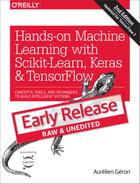
The fundamental idea behind SVMs is best explained with some pictures. Figure 5-1 shows part of the iris dataset that was introduced at the end of Chapter 4. The two classes can clearly be separated easily with a straight line (they are linearly separable). The left plot shows the decision boundaries of three possible linear classifiers. The model whose decision boundary is represented by the dashed line is so bad that it does not even separate the classes properly. The other two models work perfectly on this training set, but their decision boundaries come so close to the instances that these models will probably not perform as well on new instances. In contrast, the solid line in the plot on the right represents the decision boundary of an SVM classifier; this line not only separates the two classes but also stays as far away from the closest training instances as possible. You can think of an SVM classifier as fitting the widest possible street (represented by the parallel dashed lines) between the classes. This is called large margin classification.
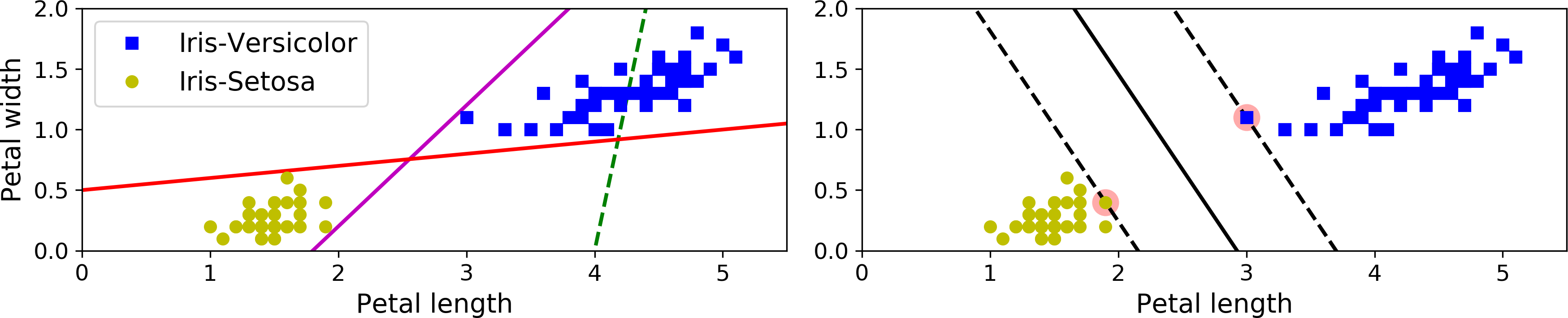
Figure 5-1. Large margin classification
Notice that adding more training instances “off the street” will not affect the decision boundary at all: it is fully determined (or “supported”) by the instances located on the edge of the street. These instances are called the support vectors (they are circled in Figure 5-1).
Warning
SVMs are sensitive to the feature scales, as you can see in Figure 5-2: on the left plot, the vertical scale is much larger than the horizontal scale, so the widest possible street is close to horizontal. After feature scaling (e.g., using Scikit-Learn’s StandardScaler), the decision boundary looks much better (on the right plot).
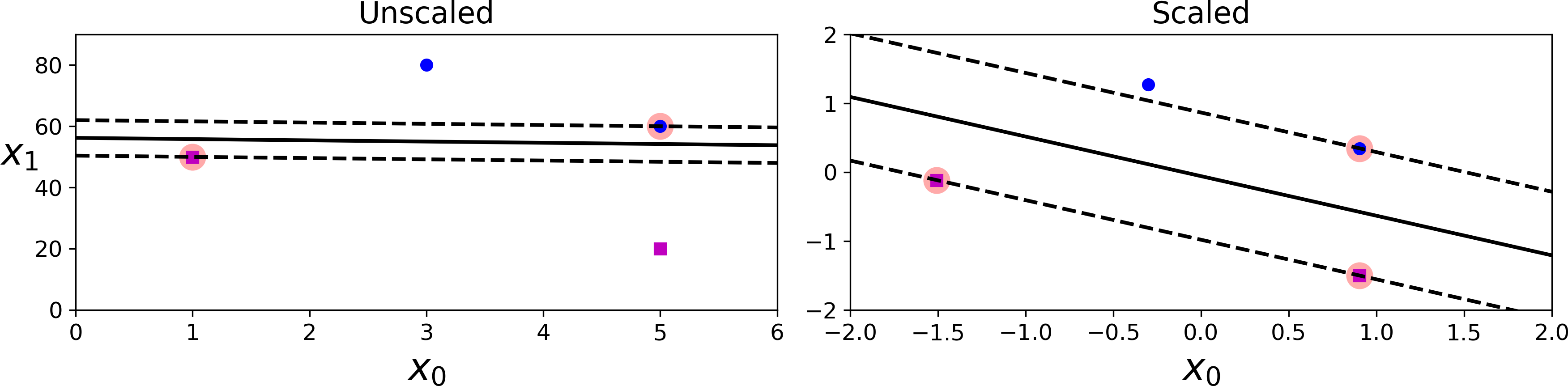
Figure 5-2. Sensitivity to feature scales
Soft Margin Classification
If we strictly impose that all instances be off the street and on the right side, this is called hard margin classification. There are two main issues with hard margin classification. First, it only works if the data is linearly separable, and second it is quite sensitive to outliers. Figure 5-3 shows the iris dataset with just one additional outlier: on the left, it is impossible to find a hard margin, and on the right the decision boundary ends up very different from the one we saw in Figure 5-1 without the outlier, and it will probably not generalize as well.
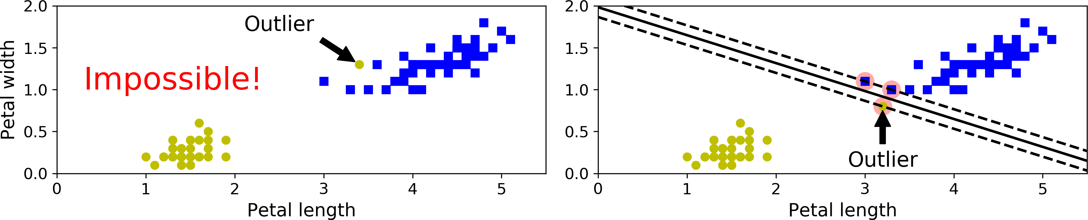
Figure 5-3. Hard margin sensitivity to outliers
To avoid these issues it is preferable to use a more flexible model. The objective is to find a good balance between keeping the street as large as possible and limiting the margin violations (i.e., instances that end up in the middle of the street or even on the wrong side). This is called soft margin classification.
In Scikit-Learn’s SVM classes, you can control this balance using the C hyperparameter: a smaller C value leads to a wider street but more margin violations. Figure 5-4 shows the decision boundaries and margins of two soft margin SVM classifiers on a nonlinearly separable dataset. On the right, using a low C value the margin is quite large, but many instances end up on the street. On the left, using a high C value the classifier makes fewer margin violations but ends up with a smaller margin. However, it seems likely that the first classifier will generalize better: in fact even on this training set it makes fewer prediction errors, since most of the margin violations are actually on the correct side of the decision boundary.
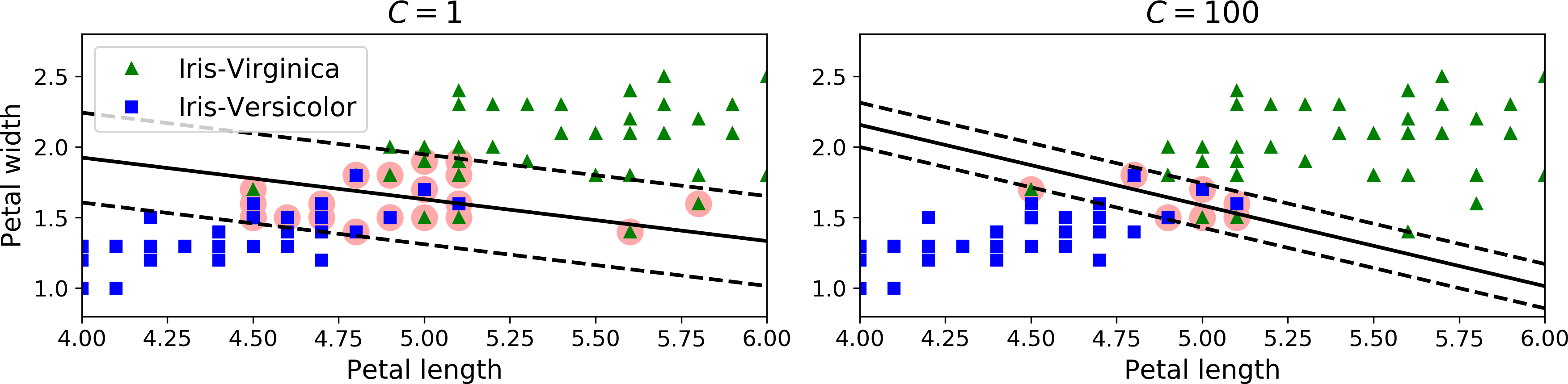
Figure 5-4. Large margin (left) versus fewer margin violations (right)
The following Scikit-Learn code loads the iris dataset, scales the features, and then trains a linear SVM model (using the LinearSVC class with C = 1 and the hinge loss function, described shortly) to detect Iris-Virginica flowers. The resulting model is represented on the left of Figure 5-4.
importnumpyasnpfromsklearnimportdatasetsfromsklearn.pipelineimportPipelinefromsklearn.preprocessingimportStandardScalerfromsklearn.svmimportLinearSVCiris=datasets.load_iris()X=iris["data"][:,(2,3)]# petal length, petal widthy=(iris["target"]==2).astype(np.float64)# Iris-Virginicasvm_clf=Pipeline([("scaler",StandardScaler()),("linear_svc",LinearSVC(C=1,loss="hinge")),])svm_clf.fit(X,y)
Then, as usual, you can use the model to make predictions:
>>>svm_clf.predict([[5.5,1.7]])array([1.])
Note
Unlike Logistic Regression classifiers, SVM classifiers do not output probabilities for each class.
Alternatively, you could use the SVC class, using SVC(kernel="linear", C=1), but it is much slower, especially with large training sets, so it is not recommended. Another option is to use the SGDClassifier class, with SGDClassifier(loss="hinge", alpha=1/(m*C)). This applies regular Stochastic Gradient Descent (see Chapter 4) to train a linear SVM classifier. It does not converge as fast as the LinearSVC class, but it can be useful to handle huge datasets that do not fit in memory (out-of-core training), or to handle online classification tasks.
Tip
The LinearSVC class regularizes the bias term, so you should center the training set first by subtracting its mean. This is automatic if you scale the data using the StandardScaler. Moreover, make sure you set the loss hyperparameter to "hinge", as it is not the default value. Finally, for better performance you should set the dual hyperparameter to False, unless there are more features than training instances (we will discuss duality later in the chapter).
Nonlinear SVM Classification
Although linear SVM classifiers are efficient and work surprisingly well in many cases, many datasets are not even close to being linearly separable. One approach to handling nonlinear datasets is to add more features, such as polynomial features (as you did in Chapter 4); in some cases this can result in a linearly separable dataset. Consider the left plot in Figure 5-5: it represents a simple dataset with just one feature x1. This dataset is not linearly separable, as you can see. But if you add a second feature x2 = (x1)2, the resulting 2D dataset is perfectly linearly separable.
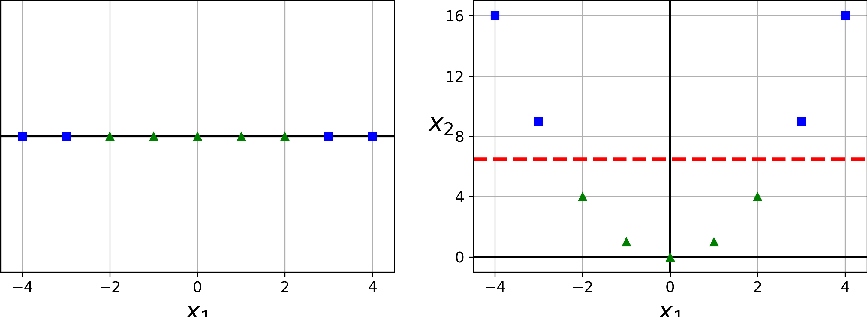
Figure 5-5. Adding features to make a dataset linearly separable
To implement this idea using Scikit-Learn, you can create a Pipeline containing a PolynomialFeatures transformer (discussed in “Polynomial Regression”), followed by a StandardScaler and a LinearSVC. Let’s test this on the moons dataset: this is a toy dataset for binary classification in which the data points are shaped as two interleaving half circles (see Figure 5-6). You can generate this dataset using the make_moons() function:
fromsklearn.datasetsimportmake_moonsfromsklearn.pipelineimportPipelinefromsklearn.preprocessingimportPolynomialFeaturespolynomial_svm_clf=Pipeline([("poly_features",PolynomialFeatures(degree=3)),("scaler",StandardScaler()),("svm_clf",LinearSVC(C=10,loss="hinge"))])polynomial_svm_clf.fit(X,y)
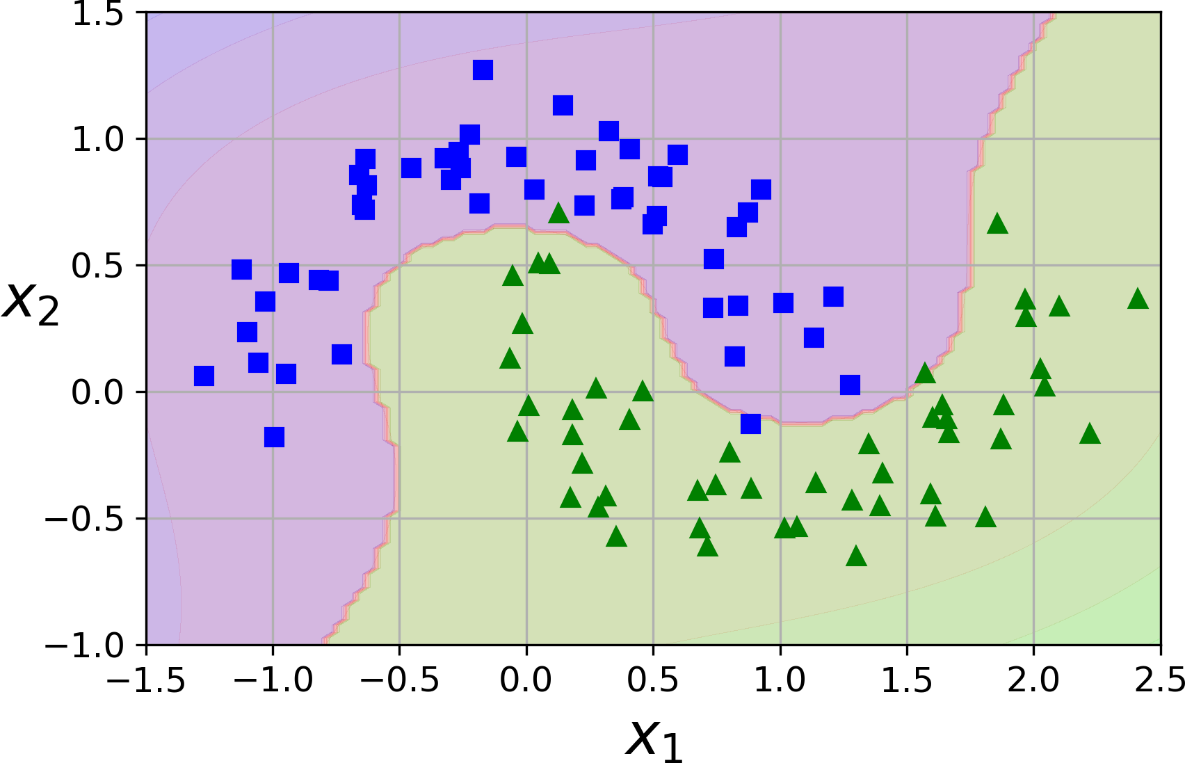
Figure 5-6. Linear SVM classifier using polynomial features
Polynomial Kernel
Adding polynomial features is simple to implement and can work great with all sorts of Machine Learning algorithms (not just SVMs), but at a low polynomial degree it cannot deal with very complex datasets, and with a high polynomial degree it creates a huge number of features, making the model too slow.
Fortunately, when using SVMs you can apply an almost miraculous mathematical technique called the kernel trick (it is explained in a moment). It makes it possible to get the same result as if you added many polynomial features, even with very high-degree polynomials, without actually having to add them. So there is no combinatorial explosion of the number of features since you don’t actually add any features. This trick is implemented by the SVC class. Let’s test it on the moons dataset:
fromsklearn.svmimportSVCpoly_kernel_svm_clf=Pipeline([("scaler",StandardScaler()),("svm_clf",SVC(kernel="poly",degree=3,coef0=1,C=5))])poly_kernel_svm_clf.fit(X,y)
This code trains an SVM classifier using a 3rd-degree polynomial kernel. It is represented on the left of Figure 5-7. On the right is another SVM classifier using a 10th-degree polynomial kernel. Obviously, if your model is overfitting, you might want to reduce the polynomial degree. Conversely, if it is underfitting, you can try increasing it. The hyperparameter coef0 controls how much the model is influenced by high-degree polynomials versus low-degree polynomials.
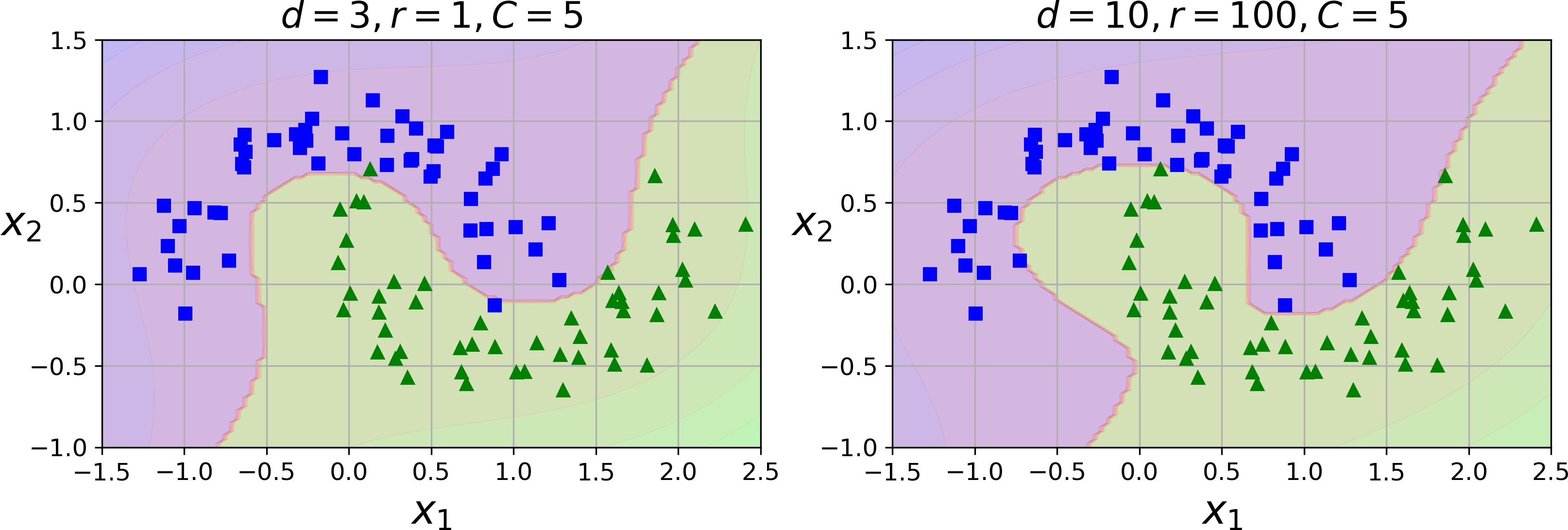
Figure 5-7. SVM classifiers with a polynomial kernel
Tip
A common approach to find the right hyperparameter values is to use grid search (see Chapter 2). It is often faster to first do a very coarse grid search, then a finer grid search around the best values found. Having a good sense of what each hyperparameter actually does can also help you search in the right part of the hyperparameter space.
Adding Similarity Features
Another technique to tackle nonlinear problems is to add features computed using a similarity function that measures how much each instance resembles a particular landmark. For example, let’s take the one-dimensional dataset discussed earlier and add two landmarks to it at x1 = –2 and x1 = 1 (see the left plot in Figure 5-8). Next, let’s define the similarity function to be the Gaussian Radial Basis Function (RBF) with γ = 0.3 (see Equation 5-1).
Equation 5-1. Gaussian RBF
It is a bell-shaped function varying from 0 (very far away from the landmark) to 1 (at the landmark). Now we are ready to compute the new features. For example, let’s look at the instance x1 = –1: it is located at a distance of 1 from the first landmark, and 2 from the second landmark. Therefore its new features are x2 = exp (–0.3 × 12) ≈ 0.74 and x3 = exp (–0.3 × 22) ≈ 0.30. The plot on the right of Figure 5-8 shows the transformed dataset (dropping the original features). As you can see, it is now linearly separable.
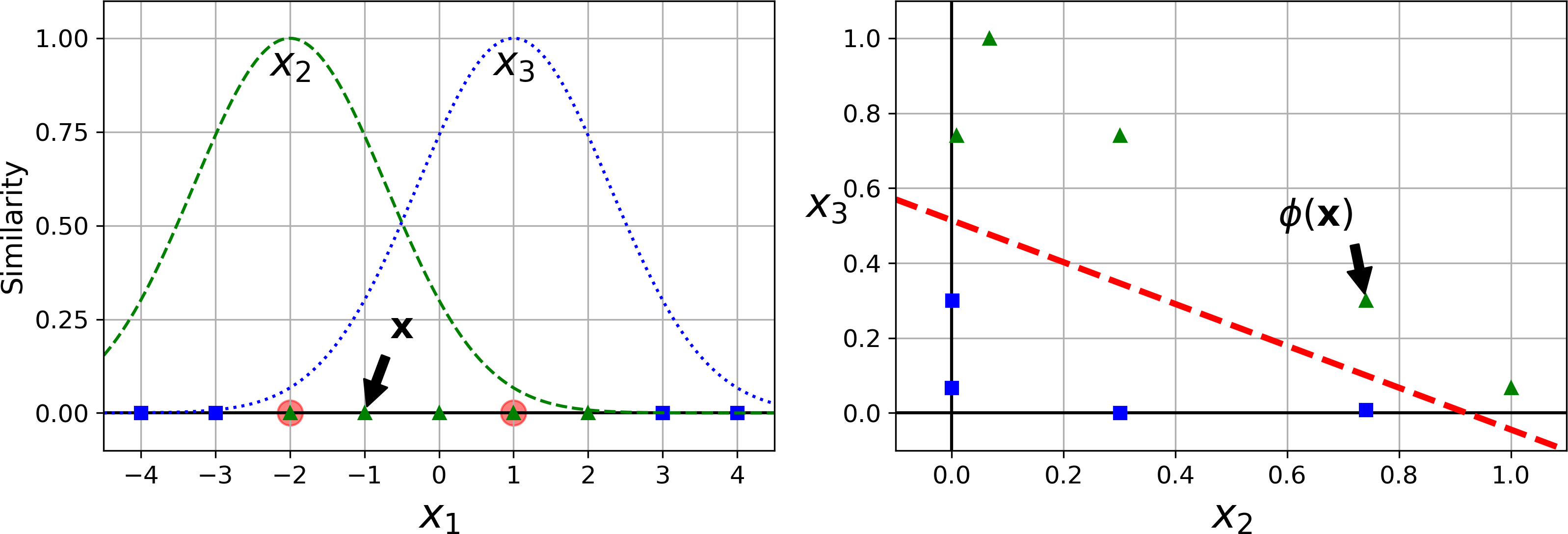
Figure 5-8. Similarity features using the Gaussian RBF
You may wonder how to select the landmarks. The simplest approach is to create a landmark at the location of each and every instance in the dataset. This creates many dimensions and thus increases the chances that the transformed training set will be linearly separable. The downside is that a training set with m instances and n features gets transformed into a training set with m instances and m features (assuming you drop the original features). If your training set is very large, you end up with an equally large number of features.
Gaussian RBF Kernel
Just like the polynomial features method, the similarity features method can be useful with any Machine Learning algorithm, but it may be computationally expensive to compute all the additional features, especially on large training sets. However, once again the kernel trick does its SVM magic: it makes it possible to obtain a similar result as if you had added many similarity features, without actually having to add them. Let’s try the Gaussian RBF kernel using the SVC class:
rbf_kernel_svm_clf=Pipeline([("scaler",StandardScaler()),("svm_clf",SVC(kernel="rbf",gamma=5,C=0.001))])rbf_kernel_svm_clf.fit(X,y)
This model is represented on the bottom left of Figure 5-9. The other plots show models trained with different values of hyperparameters gamma (γ) and C. Increasing gamma makes the bell-shape curve narrower (see the left plot of Figure 5-8), and as a result each instance’s range of influence is smaller: the decision boundary ends up being more irregular, wiggling around individual instances. Conversely, a small gamma value makes the bell-shaped curve wider, so instances have a larger range of influence, and the decision boundary ends up smoother. So γ acts like a regularization hyperparameter: if your model is overfitting, you should reduce it, and if it is underfitting, you should increase it (similar to the C hyperparameter).
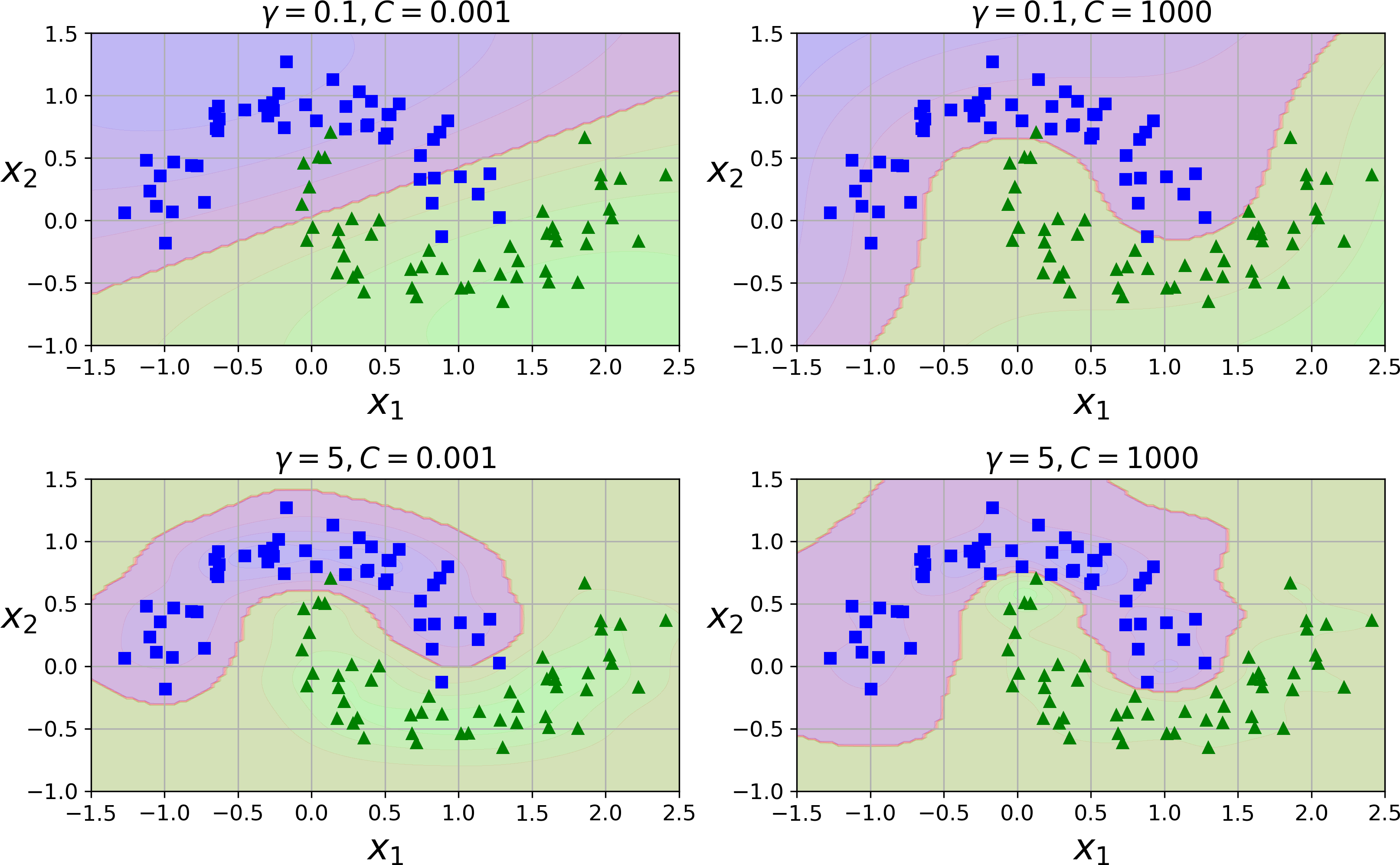
Figure 5-9. SVM classifiers using an RBF kernel
Other kernels exist but are used much more rarely. For example, some kernels are specialized for specific data structures. String kernels are sometimes used when classifying text documents or DNA sequences (e.g., using the string subsequence kernel or kernels based on the Levenshtein distance).
Tip
With so many kernels to choose from, how can you decide which one to use? As a rule of thumb, you should always try the linear kernel first (remember that LinearSVC is much faster than SVC(kernel="linear")), especially if the training set is very large or if it has plenty of features. If the training set is not too large, you should try the Gaussian RBF kernel as well; it works well in most cases. Then if you have spare time and computing power, you can also experiment with a few other kernels using cross-validation and grid search, especially if there are kernels specialized for your training set’s data structure.
Computational Complexity
The LinearSVC class is based on the liblinear library, which implements an optimized algorithm for linear SVMs.1 It does not support the kernel trick, but it scales almost linearly with the number of training instances and the number of features: its training time complexity is roughly O(m × n).
The algorithm takes longer if you require a very high precision. This is controlled by the tolerance hyperparameter ϵ (called tol in Scikit-Learn). In most classification tasks, the default tolerance is fine.
The SVC class is based on the libsvm library, which implements an algorithm that supports the kernel trick.2 The training time complexity is usually between O(m2 × n) and O(m3 × n). Unfortunately, this means that it gets dreadfully slow when the number of training instances gets large (e.g., hundreds of thousands of instances). This algorithm is perfect for complex but small or medium training sets. However, it scales well with the number of features, especially with sparse features (i.e., when each instance has few nonzero features). In this case, the algorithm scales roughly with the average number of nonzero features per instance. Table 5-1 compares Scikit-Learn’s SVM classification classes.
SVM Regression
As we mentioned earlier, the SVM algorithm is quite versatile: not only does it support linear and nonlinear classification, but it also supports linear and nonlinear regression. The trick is to reverse the objective: instead of trying to fit the largest possible street between two classes while limiting margin violations, SVM Regression tries to fit as many instances as possible on the street while limiting margin violations (i.e., instances off the street). The width of the street is controlled by a hyperparameter ϵ. Figure 5-10 shows two linear SVM Regression models trained on some random linear data, one with a large margin (ϵ = 1.5) and the other with a small margin (ϵ = 0.5).
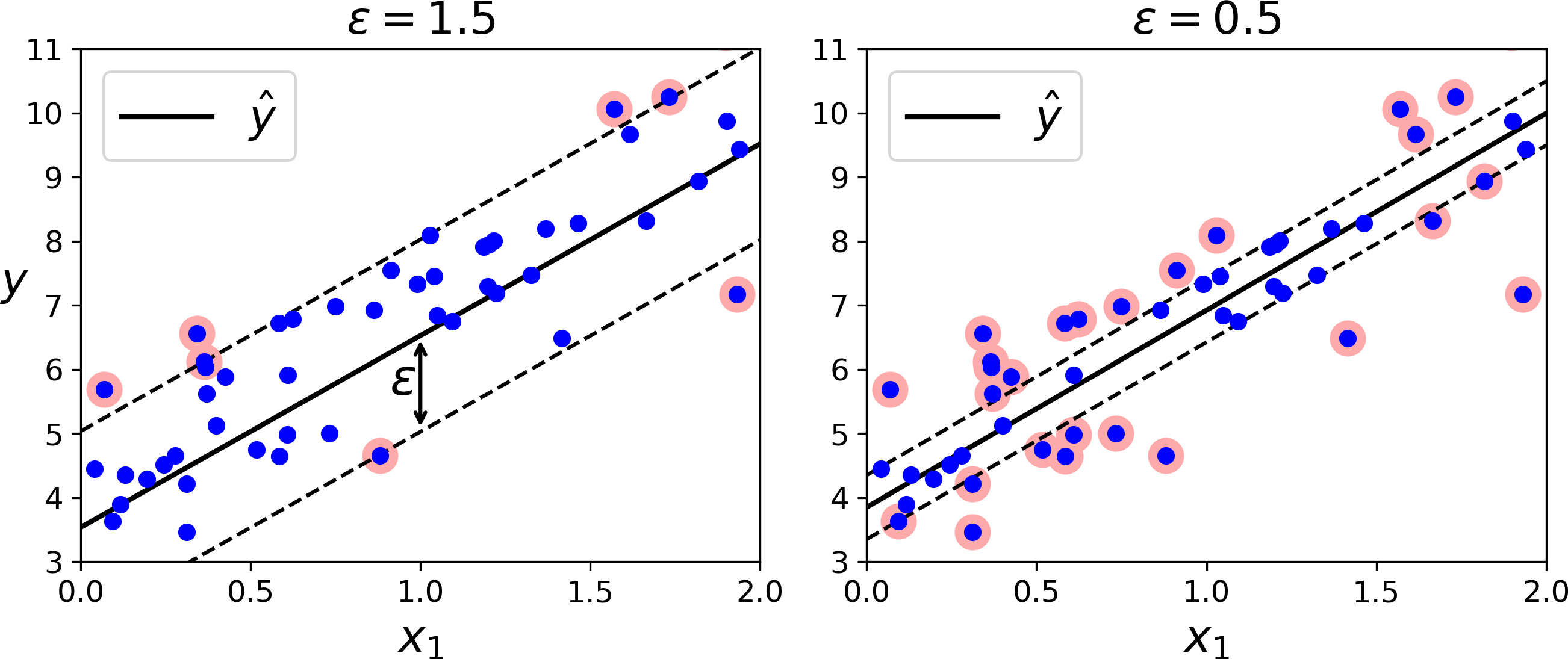
Figure 5-10. SVM Regression
Adding more training instances within the margin does not affect the model’s predictions; thus, the model is said to be ϵ-insensitive.
You can use Scikit-Learn’s LinearSVR class to perform linear SVM Regression. The following code produces the model represented on the left of Figure 5-10 (the training data should be scaled and centered first):
fromsklearn.svmimportLinearSVRsvm_reg=LinearSVR(epsilon=1.5)svm_reg.fit(X,y)
To tackle nonlinear regression tasks, you can use a kernelized SVM model. For example, Figure 5-11 shows SVM Regression on a random quadratic training set, using a 2nd-degree polynomial kernel. There is little regularization on the left plot (i.e., a large C value), and much more regularization on the right plot (i.e., a small C value).
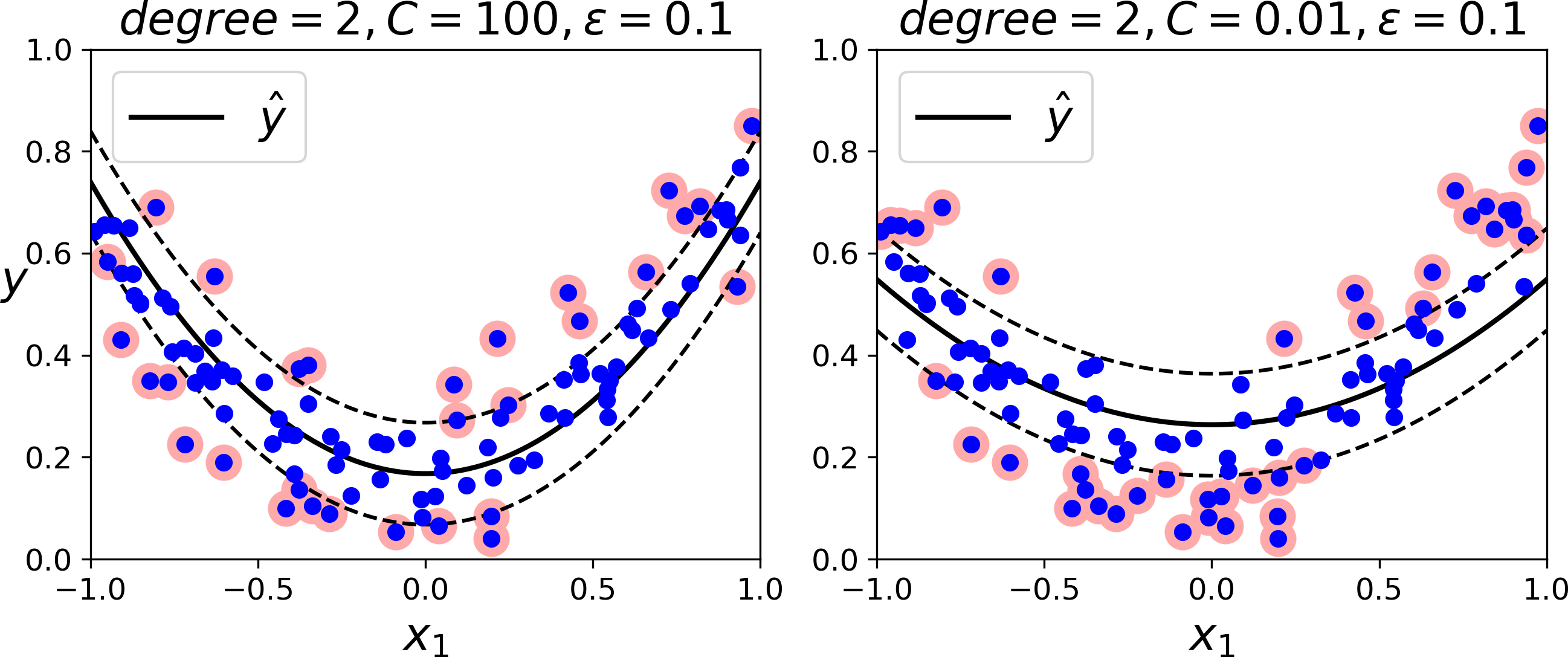
Figure 5-11. SVM regression using a 2nd-degree polynomial kernel
The following code produces the model represented on the left of Figure 5-11 using Scikit-Learn’s SVR class (which supports the kernel trick). The SVR class is the regression equivalent of the SVC class, and the LinearSVR class is the regression equivalent of the LinearSVC class. The LinearSVR class scales linearly with the size of the training set (just like the LinearSVC class), while the SVR class gets much too slow when the training set grows large (just like the SVC class).
fromsklearn.svmimportSVRsvm_poly_reg=SVR(kernel="poly",degree=2,C=100,epsilon=0.1)svm_poly_reg.fit(X,y)
Note
SVMs can also be used for outlier detection; see Scikit-Learn’s documentation for more details.
Under the Hood
This section explains how SVMs make predictions and how their training algorithms work, starting with linear SVM classifiers. You can safely skip it and go straight to the exercises at the end of this chapter if you are just getting started with Machine Learning, and come back later when you want to get a deeper understanding of SVMs.
First, a word about notations: in Chapter 4 we used the convention of putting all the model parameters in one vector θ, including the bias term θ0 and the input feature weights θ1 to θn, and adding a bias input x0 = 1 to all instances. In this chapter, we will use a different convention, which is more convenient (and more common) when you are dealing with SVMs: the bias term will be called b and the feature weights vector will be called w. No bias feature will be added to the input feature vectors.
Decision Function and Predictions
The linear SVM classifier model predicts the class of a new instance x by simply computing the decision function wT x + b = w1 x1 + ⋯ + wn xn + b: if the result is positive, the predicted class ŷ is the positive class (1), or else it is the negative class (0); see Equation 5-2.
Equation 5-2. Linear SVM classifier prediction
Figure 5-12 shows the decision function that corresponds to the model on the left of Figure 5-4: it is a two-dimensional plane since this dataset has two features (petal width and petal length). The decision boundary is the set of points where the decision function is equal to 0: it is the intersection of two planes, which is a straight line (represented by the thick solid line).3
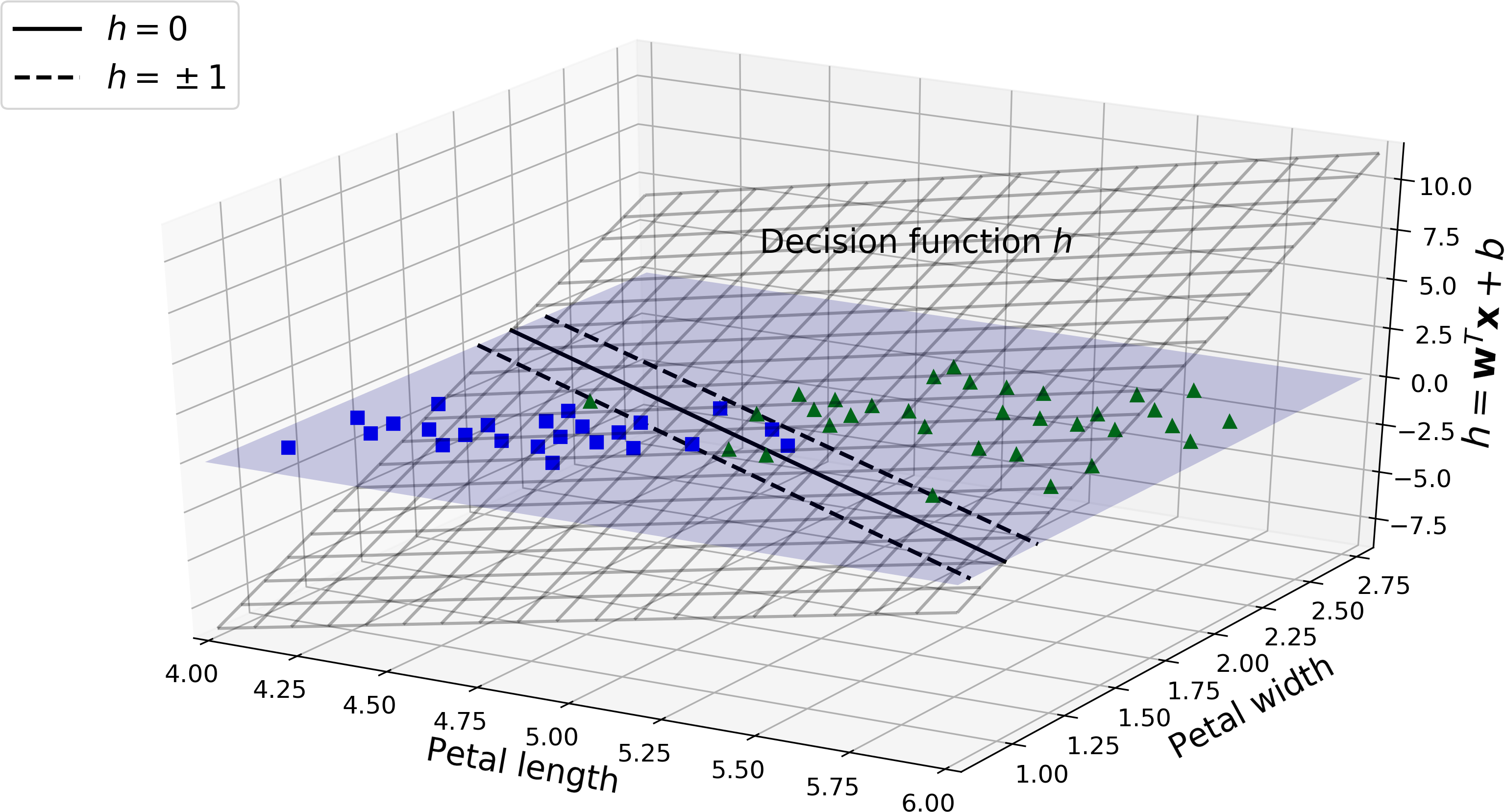
Figure 5-12. Decision function for the iris dataset
The dashed lines represent the points where the decision function is equal to 1 or –1: they are parallel and at equal distance to the decision boundary, forming a margin around it. Training a linear SVM classifier means finding the value of w and b that make this margin as wide as possible while avoiding margin violations (hard margin) or limiting them (soft margin).
Training Objective
Consider the slope of the decision function: it is equal to the norm of the weight vector, ∥ w ∥. If we divide this slope by 2, the points where the decision function is equal to ±1 are going to be twice as far away from the decision boundary. In other words, dividing the slope by 2 will multiply the margin by 2. Perhaps this is easier to visualize in 2D in Figure 5-13. The smaller the weight vector w, the larger the margin.
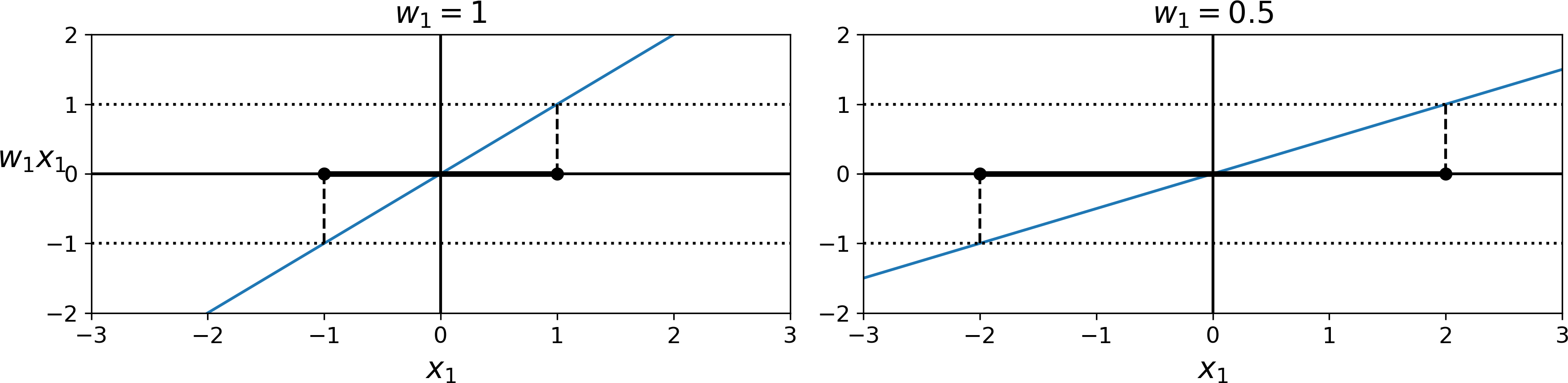
Figure 5-13. A smaller weight vector results in a larger margin
So we want to minimize ∥ w ∥ to get a large margin. However, if we also want to avoid any margin violation (hard margin), then we need the decision function to be greater than 1 for all positive training instances, and lower than –1 for negative training instances. If we define t(i) = –1 for negative instances (if y(i) = 0) and t(i) = 1 for positive instances (if y(i) = 1), then we can express this constraint as t(i)(wT x(i) + b) ≥ 1 for all instances.
We can therefore express the hard margin linear SVM classifier objective as the constrained optimization problem in Equation 5-3.
Equation 5-3. Hard margin linear SVM classifier objective
Note
We are minimizing wT w, which is equal to ∥ w ∥2, rather than minimizing ∥ w ∥. Indeed, ∥ w ∥2 has a nice and simple derivative (it is just w) while ∥ w ∥ is not differentiable at w = 0. Optimization algorithms work much better on differentiable functions.
To get the soft margin objective, we need to introduce a slack variable ζ(i) ≥ 0 for each instance:4 ζ(i) measures how much the ith instance is allowed to violate the margin. We now have two conflicting objectives: making the slack variables as small as possible to reduce the margin violations, and making wT w as small as possible to increase the margin. This is where the C hyperparameter comes in: it allows us to define the tradeoff between these two objectives. This gives us the constrained optimization problem in Equation 5-4.
Equation 5-4. Soft margin linear SVM classifier objective
Quadratic Programming
The hard margin and soft margin problems are both convex quadratic optimization problems with linear constraints. Such problems are known as Quadratic Programming (QP) problems. Many off-the-shelf solvers are available to solve QP problems using a variety of techniques that are outside the scope of this book.5 The general problem formulation is given by Equation 5-5.
Equation 5-5. Quadratic Programming problem
Note that the expression A p ≤ b actually defines nc constraints: pT a(i) ≤ b(i) for i = 1, 2, ⋯, nc, where a(i) is the vector containing the elements of the ith row of A and b(i) is the ith element of b.
You can easily verify that if you set the QP parameters in the following way, you get the hard margin linear SVM classifier objective:
-
np = n + 1, where n is the number of features (the +1 is for the bias term).
-
nc = m, where m is the number of training instances.
-
H is the np × np identity matrix, except with a zero in the top-left cell (to ignore the bias term).
-
f = 0, an np-dimensional vector full of 0s.
-
b = –1, an nc-dimensional vector full of –1s.
-
a(i) = –t(i) (i), where (i) is equal to x(i) with an extra bias feature 0 = 1.
So one way to train a hard margin linear SVM classifier is just to use an off-the-shelf QP solver by passing it the preceding parameters. The resulting vector p will contain the bias term b = p0 and the feature weights wi = pi for i = 1, 2, ⋯, n. Similarly, you can use a QP solver to solve the soft margin problem (see the exercises at the end of the chapter).
However, to use the kernel trick we are going to look at a different constrained optimization problem.
The Dual Problem
Given a constrained optimization problem, known as the primal problem, it is possible to express a different but closely related problem, called its dual problem. The solution to the dual problem typically gives a lower bound to the solution of the primal problem, but under some conditions it can even have the same solutions as the primal problem. Luckily, the SVM problem happens to meet these conditions,6 so you can choose to solve the primal problem or the dual problem; both will have the same solution. Equation 5-6 shows the dual form of the linear SVM objective (if you are interested in knowing how to derive the dual problem from the primal problem, see Appendix C).
Equation 5-6. Dual form of the linear SVM objective
Once you find the vector that minimizes this equation (using a QP solver), you can compute and that minimize the primal problem by using Equation 5-7.
Equation 5-7. From the dual solution to the primal solution
The dual problem is faster to solve than the primal when the number of training instances is smaller than the number of features. More importantly, it makes the kernel trick possible, while the primal does not. So what is this kernel trick anyway?
Kernelized SVM
Suppose you want to apply a 2nd-degree polynomial transformation to a two-dimensional training set (such as the moons training set), then train a linear SVM classifier on the transformed training set. Equation 5-8 shows the 2nd-degree polynomial mapping function ϕ that you want to apply.
Equation 5-8. Second-degree polynomial mapping
Notice that the transformed vector is three-dimensional instead of two-dimensional. Now let’s look at what happens to a couple of two-dimensional vectors, a and b, if we apply this 2nd-degree polynomial mapping and then compute the dot product7 of the transformed vectors (See Equation 5-9).
Equation 5-9. Kernel trick for a 2nd-degree polynomial mapping
How about that? The dot product of the transformed vectors is equal to the square of the dot product of the original vectors: ϕ(a)T ϕ(b) = (aT b)2.
Now here is the key insight: if you apply the transformation ϕ to all training instances, then the dual problem (see Equation 5-6) will contain the dot product ϕ(x(i))T ϕ(x(j)). But if ϕ is the 2nd-degree polynomial transformation defined in Equation 5-8, then you can replace this dot product of transformed vectors simply by . So you don’t actually need to transform the training instances at all: just replace the dot product by its square in Equation 5-6. The result will be strictly the same as if you went through the trouble of actually transforming the training set then fitting a linear SVM algorithm, but this trick makes the whole process much more computationally efficient. This is the essence of the kernel trick.
The function K(a, b) = (aT b)2 is called a 2nd-degree polynomial kernel. In Machine Learning, a kernel is a function capable of computing the dot product ϕ(a)T ϕ(b) based only on the original vectors a and b, without having to compute (or even to know about) the transformation ϕ. Equation 5-10 lists some of the most commonly used kernels.
Equation 5-10. Common kernels
There is still one loose end we must tie. Equation 5-7 shows how to go from the dual solution to the primal solution in the case of a linear SVM classifier, but if you apply the kernel trick you end up with equations that include ϕ(x(i)). In fact, must have the same number of dimensions as ϕ(x(i)), which may be huge or even infinite, so you can’t compute it. But how can you make predictions without knowing ? Well, the good news is that you can plug in the formula for from Equation 5-7 into the decision function for a new instance x(n), and you get an equation with only dot products between input vectors. This makes it possible to use the kernel trick, once again (Equation 5-11).
Equation 5-11. Making predictions with a kernelized SVM
Note that since α(i) ≠ 0 only for support vectors, making predictions involves computing the dot product of the new input vector x(n) with only the support vectors, not all the training instances. Of course, you also need to compute the bias term , using the same trick (Equation 5-12).
Equation 5-12. Computing the bias term using the kernel trick
If you are starting to get a headache, it’s perfectly normal: it’s an unfortunate side effect of the kernel trick.
Online SVMs
Before concluding this chapter, let’s take a quick look at online SVM classifiers (recall that online learning means learning incrementally, typically as new instances arrive).
For linear SVM classifiers, one method is to use Gradient Descent (e.g., using SGDClassifier) to minimize the cost function in Equation 5-13, which is derived from the primal problem. Unfortunately it converges much more slowly than the methods based on QP.
Equation 5-13. Linear SVM classifier cost function
The first sum in the cost function will push the model to have a small weight vector w, leading to a larger margin. The second sum computes the total of all margin violations. An instance’s margin violation is equal to 0 if it is located off the street and on the correct side, or else it is proportional to the distance to the correct side of the street. Minimizing this term ensures that the model makes the margin violations as small and as few as possible
It is also possible to implement online kernelized SVMs—for example, using “Incremental and Decremental SVM Learning”8 or “Fast Kernel Classifiers with Online and Active Learning.”9 However, these are implemented in Matlab and C++. For large-scale nonlinear problems, you may want to consider using neural networks instead (see Part II).
Exercises
-
What is the fundamental idea behind Support Vector Machines?
-
What is a support vector?
-
Why is it important to scale the inputs when using SVMs?
-
Can an SVM classifier output a confidence score when it classifies an instance? What about a probability?
-
Should you use the primal or the dual form of the SVM problem to train a model on a training set with millions of instances and hundreds of features?
-
Say you trained an SVM classifier with an RBF kernel. It seems to underfit the training set: should you increase or decrease γ (
gamma)? What aboutC? -
How should you set the QP parameters (H, f, A, and b) to solve the soft margin linear SVM classifier problem using an off-the-shelf QP solver?
-
Train a
LinearSVCon a linearly separable dataset. Then train anSVCand aSGDClassifieron the same dataset. See if you can get them to produce roughly the same model. -
Train an SVM classifier on the MNIST dataset. Since SVM classifiers are binary classifiers, you will need to use one-versus-all to classify all 10 digits. You may want to tune the hyperparameters using small validation sets to speed up the process. What accuracy can you reach?
Solutions to these exercises are available in Appendix A.
1 “A Dual Coordinate Descent Method for Large-scale Linear SVM,” Lin et al. (2008).
2 “Sequential Minimal Optimization (SMO),” J. Platt (1998).
3 More generally, when there are n features, the decision function is an n-dimensional hyperplane, and the decision boundary is an (n – 1)-dimensional hyperplane.
4 Zeta (ζ) is the 6th letter of the Greek alphabet.
5 To learn more about Quadratic Programming, you can start by reading Stephen Boyd and Lieven Vandenberghe, Convex Optimization (Cambridge, UK: Cambridge University Press, 2004) or watch Richard Brown’s series of video lectures.
6 The objective function is convex, and the inequality constraints are continuously differentiable and convex functions.
7 As explained in Chapter 4, the dot product of two vectors a and b is normally noted a · b. However, in Machine Learning, vectors are frequently represented as column vectors (i.e., single-column matrices), so the dot product is achieved by computing aTb. To remain consistent with the rest of the book, we will use this notation here, ignoring the fact that this technically results in a single-cell matrix rather than a scalar value.
8 “Incremental and Decremental Support Vector Machine Learning,” G. Cauwenberghs, T. Poggio (2001).
9 “Fast Kernel Classifiers with Online and Active Learning,“ A. Bordes, S. Ertekin, J. Weston, L. Bottou (2005).