MNIST

In this chapter, we will be using the MNIST dataset, which is a set of 70,000 small images of digits handwritten by high school students and employees of the US Census Bureau. Each image is labeled with the digit it represents. This set has been studied so much that it is often called the “Hello World” of Machine Learning: whenever people come up with a new classification algorithm, they are curious to see how it will perform on MNIST. Whenever someone learns Machine Learning, sooner or later they tackle MNIST.

Scikit-Learn provides many helper functions to download popular datasets. MNIST is one of them. The following code fetches the MNIST dataset:¹

>>> from sklearn.datasets import fetch_openml
>>> mnist = fetch_openml('mnist_784', version=1)
>>> mnist.keys()
dict_keys(['data', 'target', 'feature_names', 'DESCR', 'details',
           'categories', 'url'])

Datasets loaded by Scikit-Learn generally have a similar dictionary structure including:

• A DESCR key describing the dataset

• A data key containing an array with one row per instance and one column per feature

• A target key containing an array with the labels

Let’s look at these arrays:

>>> X, y = mnist["data"], mnist["target"]
>>> X.shape
(70000, 784)
>>> y.shape
(70000,)

There are 70,000 images, and each image has 784 features. This is because each image is 28×28 pixels, and each feature simply represents one pixel’s intensity, from 0 (white) to 255 (black). Let’s take a peek at one digit from the dataset. All you need to do is grab an instance’s feature vector, reshape it to a 28×28 array, and display it using Matplotlib’s imshow() function:

import matplotlib as mpl
import matplotlib.pyplot as plt

some_digit = X[0]
some_digit_image = some_digit.reshape(28, 28)

plt.imshow(some_digit_image, cmap = mpl.cm.binary, interpolation="nearest")
plt.axis("off")
plt.show()

This looks like a 5, and indeed that’s what the label tells us:

>>> y[0]
'5'

Note that the label is a string. We prefer numbers, so let’s cast y to integers:

>>> y = y.astype(np.uint8)

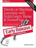
Figure 3-1 shows a few more images from the MNIST dataset to give you a feel for the complexity of the classification task.

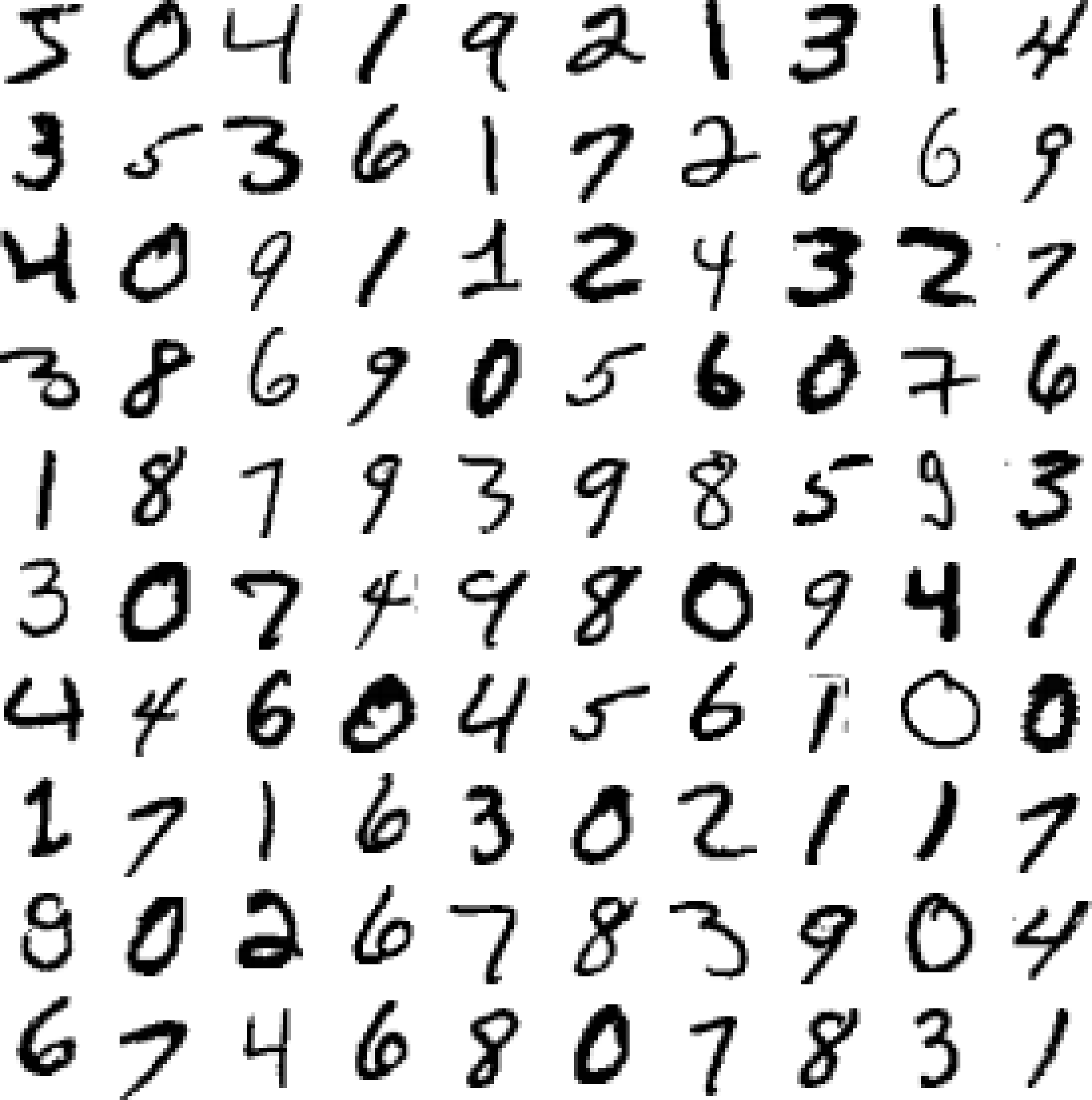
Figure 3-1. A few digits from the MNIST dataset

But wait! You should always create a test set and set it aside before inspecting the data closely. The MNIST dataset is actually already split into a training set (the first 60,000 images) and a test set (the last 10,000 images):

X_train, X_test, y_train, y_test = X[:60000], X[60000:], y[:60000], y[60000:]

The training set is already shuffled for us, which is good as this guarantees that all cross-validation folds will be similar (you don’t want one fold to be missing some digits). Moreover, some learning algorithms are sensitive to the order of the training instances, and they perform poorly if they get many similar instances in a row. Shuffling the dataset ensures that this won’t happen.²

Training a Binary Classifier

Let’s simplify the problem for now and only try to identify one digit—for example, the number 5. This “5-detector” will be an example of a binary classifier, capable of distinguishing between just two classes, 5 and not-5. Let’s create the target vectors for this classification task:

y_train_5 = (y_train == 5)  # True for all 5s, False for all other digits.
y_test_5 = (y_test == 5)

Okay, now let’s pick a classifier and train it. A good place to start is with a Stochastic Gradient Descent (SGD) classifier, using Scikit-Learn’s SGDClassifier class. This classifier has the advantage of being capable of handling very large datasets efficiently. This is in part because SGD deals with training instances independently, one at a time (which also makes SGD well suited for online learning), as we will see later. Let’s create an SGDClassifier and train it on the whole training set:

from sklearn.linear_model import SGDClassifier

sgd_clf = SGDClassifier(random_state=42)
sgd_clf.fit(X_train, y_train_5)

Now you can use it to detect images of the number 5:

>>> sgd_clf.predict([some_digit])
array([ True])

The classifier guesses that this image represents a 5 (True). Looks like it guessed right in this particular case! Now, let’s evaluate this model’s performance.

Performance Measures

Evaluating a classifier is often significantly trickier than evaluating a regressor, so we will spend a large part of this chapter on this topic. There are many performance measures available, so grab another coffee and get ready to learn many new concepts and acronyms!

>>> from sklearn.model_selection import cross_val_score
>>> cross_val_score(sgd_clf, X_train, y_train_5, cv=3, scoring="accuracy")
array([0.96355, 0.93795, 0.95615])

from sklearn.base import BaseEstimator

class Never5Classifier(BaseEstimator):
    def fit(self, X, y=None):
        pass
    def predict(self, X):
        return np.zeros((len(X), 1), dtype=bool)

>>> never_5_clf = Never5Classifier()
>>> cross_val_score(never_5_clf, X_train, y_train_5, cv=3, scoring="accuracy")
array([0.91125, 0.90855, 0.90915])

Confusion Matrix

A much better way to evaluate the performance of a classifier is to look at the confusion matrix. The general idea is to count the number of times instances of class A are classified as class B. For example, to know the number of times the classifier confused images of 5s with 3s, you would look in the 5^th row and 3^rd column of the confusion matrix.

To compute the confusion matrix, you first need to have a set of predictions, so they can be compared to the actual targets. You could make predictions on the test set, but let’s keep it untouched for now (remember that you want to use the test set only at the very end of your project, once you have a classifier that you are ready to launch). Instead, you can use the cross_val_predict() function:

from sklearn.model_selection import cross_val_predict

y_train_pred = cross_val_predict(sgd_clf, X_train, y_train_5, cv=3)

Just like the cross_val_score() function, cross_val_predict() performs K-fold cross-validation, but instead of returning the evaluation scores, it returns the predictions made on each test fold. This means that you get a clean prediction for each instance in the training set (“clean” meaning that the prediction is made by a model that never saw the data during training).

Now you are ready to get the confusion matrix using the confusion_matrix() function. Just pass it the target classes (y_train_5) and the predicted classes (y_train_pred):

>>> from sklearn.metrics import confusion_matrix
>>> confusion_matrix(y_train_5, y_train_pred)
array([[53057,  1522],
       [ 1325,  4096]])

Each row in a confusion matrix represents an actual class, while each column represents a predicted class. The first row of this matrix considers non-5 images (the negative class): 53,057 of them were correctly classified as non-5s (they are called true negatives), while the remaining 1,522 were wrongly classified as 5s (false positives). The second row considers the images of 5s (the positive class): 1,325 were wrongly classified as non-5s (false negatives), while the remaining 4,096 were correctly classified as 5s (true positives). A perfect classifier would have only true positives and true negatives, so its confusion matrix would have nonzero values only on its main diagonal (top left to bottom right):

>>> y_train_perfect_predictions = y_train_5  # pretend we reached perfection
>>> confusion_matrix(y_train_5, y_train_perfect_predictions)
array([[54579,     0],
       [    0,  5421]])

The confusion matrix gives you a lot of information, but sometimes you may prefer a more concise metric. An interesting one to look at is the accuracy of the positive predictions; this is called the precision of the classifier (Equation 3-1).

Equation 3-1. Precision

$$\text{precision}=\frac{TP}{TP+FP}$$

TP is the number of true positives, and FP is the number of false positives.

A trivial way to have perfect precision is to make one single positive prediction and ensure it is correct (precision = 1/1 = 100%). This would not be very useful since the classifier would ignore all but one positive instance. So precision is typically used along with another metric named recall, also called sensitivity or true positive rate (TPR): this is the ratio of positive instances that are correctly detected by the classifier (Equation 3-2).

Equation 3-2. Recall

$$\text{recall}=\frac{TP}{TP+FN}$$

FN is of course the number of false negatives.

If you are confused about the confusion matrix, Figure 3-2 may help.

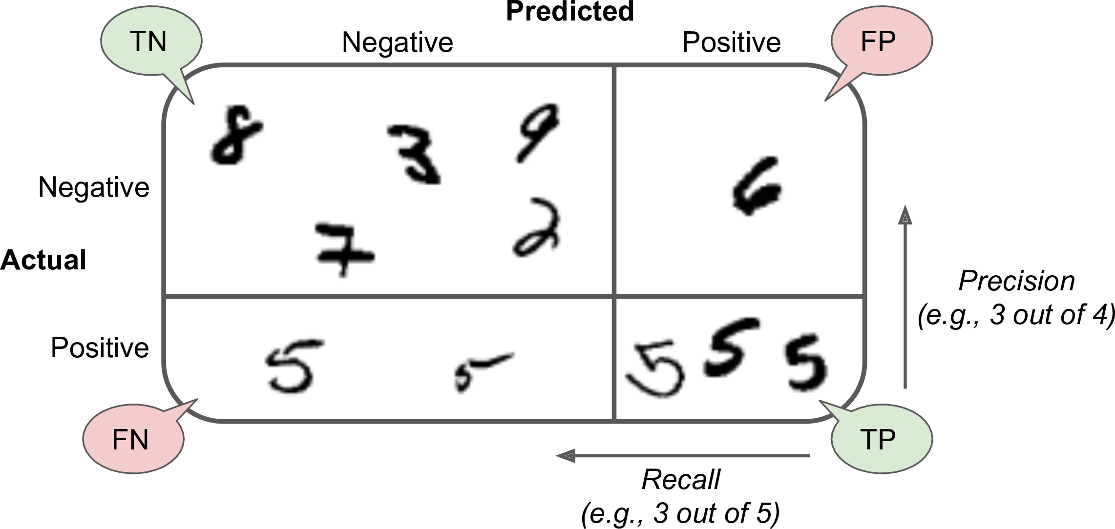
Figure 3-2. An illustrated confusion matrix

>>> from sklearn.metrics import precision_score, recall_score
>>> precision_score(y_train_5, y_train_pred) # == 4096 / (4096 + 1522)
0.7290850836596654
>>> recall_score(y_train_5, y_train_pred) # == 4096 / (4096 + 1325)
0.7555801512636044

>>> from sklearn.metrics import f1_score
>>> f1_score(y_train_5, y_train_pred)
0.7420962043663375

Precision/Recall Tradeoff

To understand this tradeoff, let’s look at how the SGDClassifier makes its classification decisions. For each instance, it computes a score based on a decision function, and if that score is greater than a threshold, it assigns the instance to the positive class, or else it assigns it to the negative class. Figure 3-3 shows a few digits positioned from the lowest score on the left to the highest score on the right. Suppose the decision threshold is positioned at the central arrow (between the two 5s): you will find 4 true positives (actual 5s) on the right of that threshold, and one false positive (actually a 6). Therefore, with that threshold, the precision is 80% (4 out of 5). But out of 6 actual 5s, the classifier only detects 4, so the recall is 67% (4 out of 6). Now if you raise the threshold (move it to the arrow on the right), the false positive (the 6) becomes a true negative, thereby increasing precision (up to 100% in this case), but one true positive becomes a false negative, decreasing recall down to 50%. Conversely, lowering the threshold increases recall and reduces precision.

Figure 3-3. Decision threshold and precision/recall tradeoff

Scikit-Learn does not let you set the threshold directly, but it does give you access to the decision scores that it uses to make predictions. Instead of calling the classifier’s predict() method, you can call its decision_function() method, which returns a score for each instance, and then make predictions based on those scores using any threshold you want:

>>> y_scores = sgd_clf.decision_function([some_digit])
>>> y_scores
array([2412.53175101])
>>> threshold = 0
>>> y_some_digit_pred = (y_scores > threshold)
array([ True])

The SGDClassifier uses a threshold equal to 0, so the previous code returns the same result as the predict() method (i.e., True). Let’s raise the threshold:

>>> threshold = 8000
>>> y_some_digit_pred = (y_scores > threshold)
>>> y_some_digit_pred
array([ True])

This confirms that raising the threshold decreases recall. The image actually represents a 5, and the classifier detects it when the threshold is 0, but it misses it when the threshold is increased to 8,000.

Now how do you decide which threshold to use? For this you will first need to get the scores of all instances in the training set using the cross_val_predict() function again, but this time specifying that you want it to return decision scores instead of predictions:

y_scores = cross_val_predict(sgd_clf, X_train, y_train_5, cv=3,
                             method="decision_function")

Now with these scores you can compute precision and recall for all possible thresholds using the precision_recall_curve() function:

from sklearn.metrics import precision_recall_curve

precisions, recalls, thresholds = precision_recall_curve(y_train_5, y_scores)

Finally, you can plot precision and recall as functions of the threshold value using Matplotlib (Figure 3-4):

def plot_precision_recall_vs_threshold(precisions, recalls, thresholds):
    plt.plot(thresholds, precisions[:-1], "b--", label="Precision")
    plt.plot(thresholds, recalls[:-1], "g-", label="Recall")
    [...] # highlight the threshold, add the legend, axis label and grid

plot_precision_recall_vs_threshold(precisions, recalls, thresholds)
plt.show()

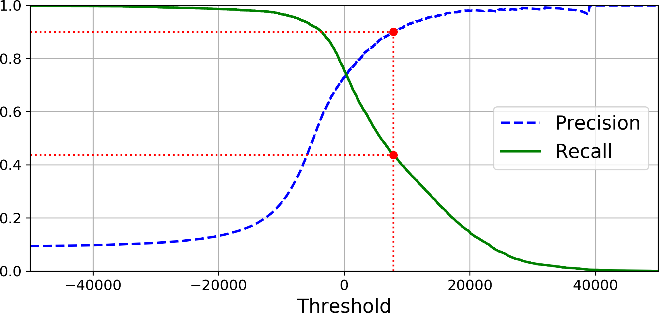
Figure 3-4. Precision and recall versus the decision threshold

Note

You may wonder why the precision curve is bumpier than the recall curve in Figure 3-4. The reason is that precision may sometimes go down when you raise the threshold (although in general it will go up). To understand why, look back at Figure 3-3 and notice what happens when you start from the central threshold and move it just one digit to the right: precision goes from 4/5 (80%) down to 3/4 (75%). On the other hand, recall can only go down when the threshold is increased, which explains why its curve looks smooth.

Another way to select a good precision/recall tradeoff is to plot precision directly against recall, as shown in Figure 3-5 (the same threshold as earlier is highlighed).

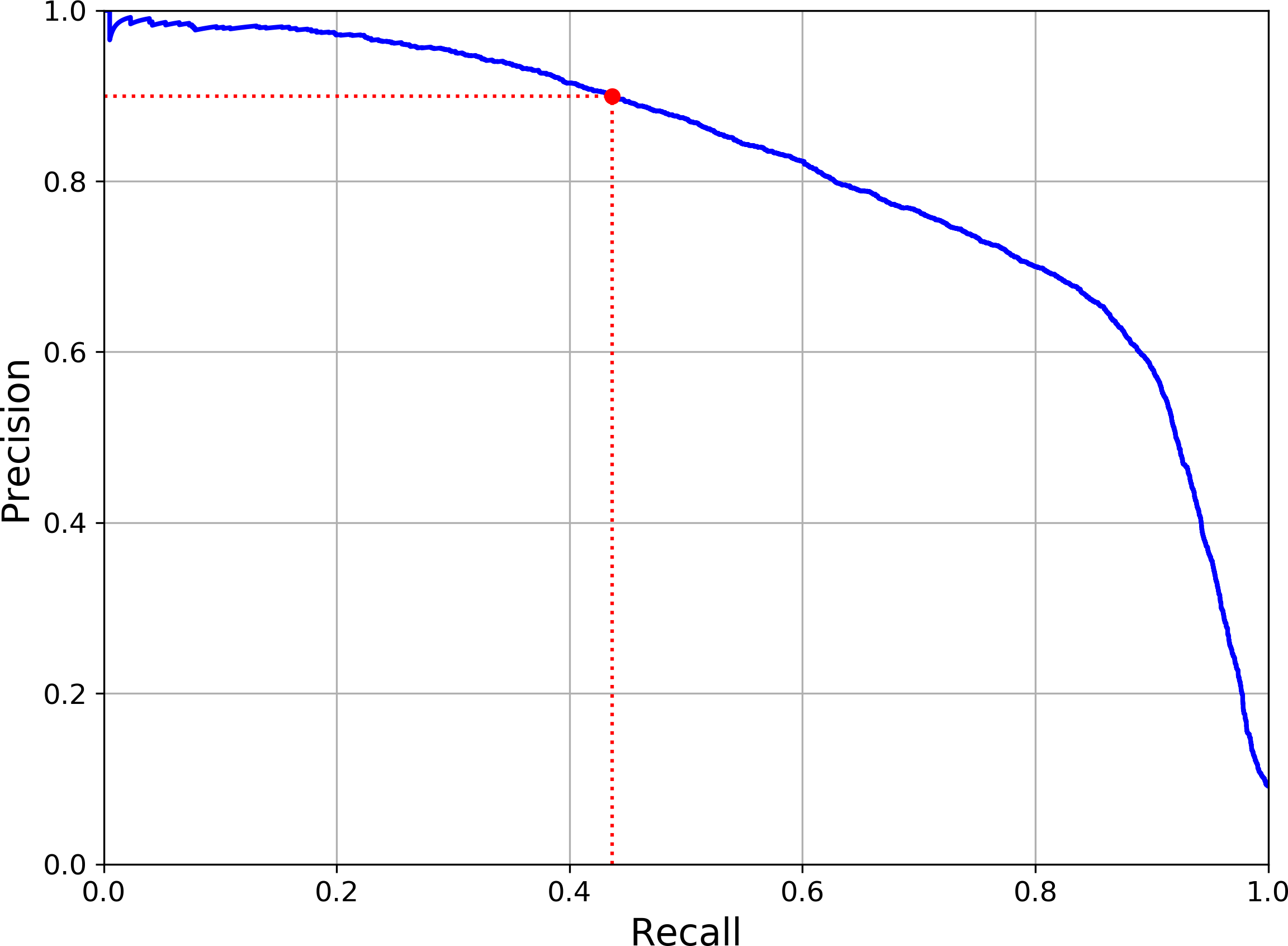
Figure 3-5. Precision versus recall

You can see that precision really starts to fall sharply around 80% recall. You will probably want to select a precision/recall tradeoff just before that drop—for example, at around 60% recall. But of course the choice depends on your project.

So let’s suppose you decide to aim for 90% precision. You look up the first plot and find that you need to use a threshold of about 8,000. To be more precise you can search for the lowest threshold that gives you at least 90% precision (np.argmax() will give us the first index of the maximum value, which in this case means the first True value):

threshold_90_precision = thresholds[np.argmax(precisions >= 0.90)] # == 7813

To make predictions (on the training set for now), instead of calling the classifier’s predict() method, you can just run this code:

y_train_pred_90 = (y_scores >= threshold_90_precision)

Let’s check these predictions’ precision and recall:

>>> precision_score(y_train_5, y_train_pred_90)
0.9000380083618396
>>> recall_score(y_train_5, y_train_pred_90)
0.4368197749492714

Great, you have a 90% precision classifier ! As you can see, it is fairly easy to create a classifier with virtually any precision you want: just set a high enough threshold, and you’re done. Hmm, not so fast. A high-precision classifier is not very useful if its recall is too low!

Tip

If someone says “let’s reach 99% precision,” you should ask, “at what recall?”

The ROC Curve

The receiver operating characteristic (ROC) curve is another common tool used with binary classifiers. It is very similar to the precision/recall curve, but instead of plotting precision versus recall, the ROC curve plots the true positive rate (another name for recall) against the false positive rate. The FPR is the ratio of negative instances that are incorrectly classified as positive. It is equal to one minus the true negative rate, which is the ratio of negative instances that are correctly classified as negative. The TNR is also called specificity. Hence the ROC curve plots sensitivity (recall) versus 1 – specificity.

To plot the ROC curve, you first need to compute the TPR and FPR for various threshold values, using the roc_curve() function:

from sklearn.metrics import roc_curve

fpr, tpr, thresholds = roc_curve(y_train_5, y_scores)

Then you can plot the FPR against the TPR using Matplotlib. This code produces the plot in Figure 3-6:

def plot_roc_curve(fpr, tpr, label=None):
    plt.plot(fpr, tpr, linewidth=2, label=label)
    plt.plot([0, 1], [0, 1], 'k--') # dashed diagonal
    [...] # Add axis labels and grid

plot_roc_curve(fpr, tpr)
plt.show()

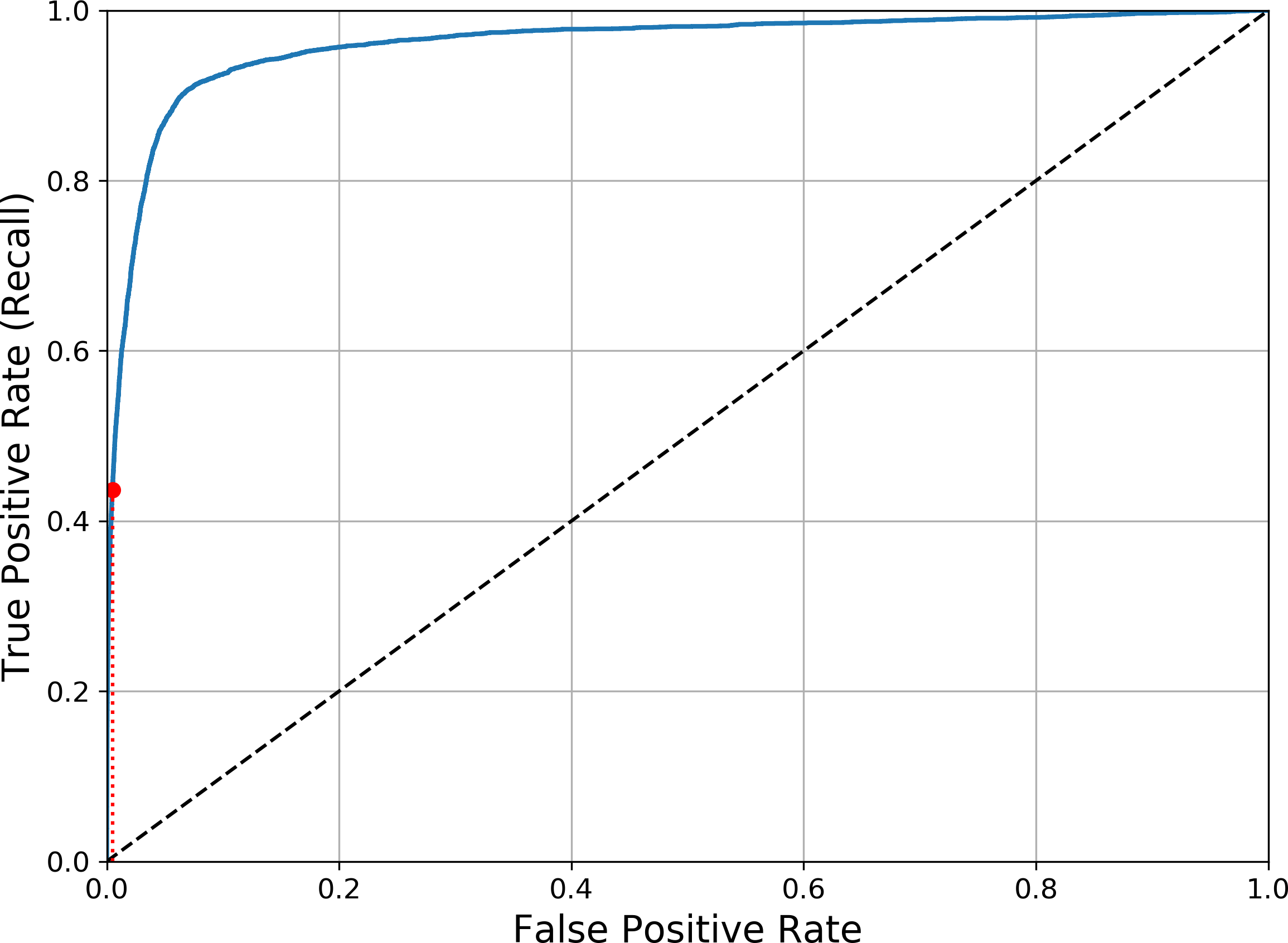
Figure 3-6. ROC curve

Once again there is a tradeoff: the higher the recall (TPR), the more false positives (FPR) the classifier produces. The dotted line represents the ROC curve of a purely random classifier; a good classifier stays as far away from that line as possible (toward the top-left corner).

One way to compare classifiers is to measure the area under the curve (AUC). A perfect classifier will have a ROC AUC equal to 1, whereas a purely random classifier will have a ROC AUC equal to 0.5. Scikit-Learn provides a function to compute the ROC AUC:

>>> from sklearn.metrics import roc_auc_score
>>> roc_auc_score(y_train_5, y_scores)
0.9611778893101814

Tip

Since the ROC curve is so similar to the precision/recall (or PR) curve, you may wonder how to decide which one to use. As a rule of thumb, you should prefer the PR curve whenever the positive class is rare or when you care more about the false positives than the false negatives, and the ROC curve otherwise. For example, looking at the previous ROC curve (and the ROC AUC score), you may think that the classifier is really good. But this is mostly because there are few positives (5s) compared to the negatives (non-5s). In contrast, the PR curve makes it clear that the classifier has room for improvement (the curve could be closer to the top-right corner).

Let’s train a RandomForestClassifier and compare its ROC curve and ROC AUC score to the SGDClassifier. First, you need to get scores for each instance in the training set. But due to the way it works (see Chapter 7), the RandomForestClassifier class does not have a decision_function() method. Instead it has a predict_proba() method. Scikit-Learn classifiers generally have one or the other. The predict_proba() method returns an array containing a row per instance and a column per class, each containing the probability that the given instance belongs to the given class (e.g., 70% chance that the image represents a 5):

from sklearn.ensemble import RandomForestClassifier

forest_clf = RandomForestClassifier(random_state=42)
y_probas_forest = cross_val_predict(forest_clf, X_train, y_train_5, cv=3,
                                    method="predict_proba")

But to plot a ROC curve, you need scores, not probabilities. A simple solution is to use the positive class’s probability as the score:

y_scores_forest = y_probas_forest[:, 1]   # score = proba of positive class
fpr_forest, tpr_forest, thresholds_forest = roc_curve(y_train_5,y_scores_forest)

Now you are ready to plot the ROC curve. It is useful to plot the first ROC curve as well to see how they compare (Figure 3-7):

plt.plot(fpr, tpr, "b:", label="SGD")
plot_roc_curve(fpr_forest, tpr_forest, "Random Forest")
plt.legend(loc="lower right")
plt.show()

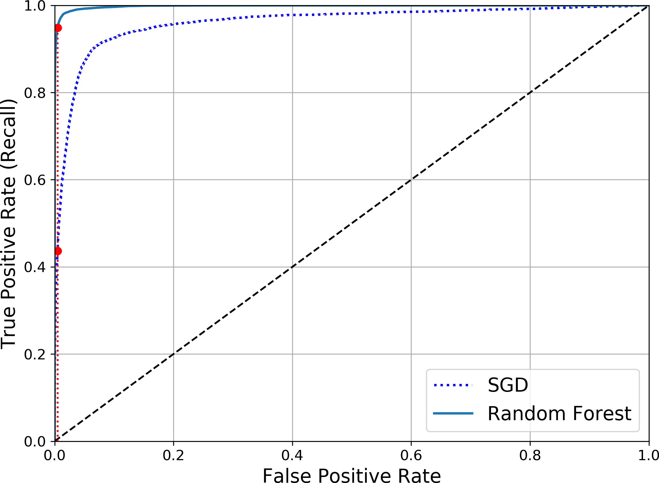
Figure 3-7. Comparing ROC curves

As you can see in Figure 3-7, the RandomForestClassifier’s ROC curve looks much better than the SGDClassifier’s: it comes much closer to the top-left corner. As a result, its ROC AUC score is also significantly better:

>>> roc_auc_score(y_train_5, y_scores_forest)
0.9983436731328145

Try measuring the precision and recall scores: you should find 99.0% precision and 86.6% recall. Not too bad!

Hopefully you now know how to train binary classifiers, choose the appropriate metric for your task, evaluate your classifiers using cross-validation, select the precision/recall tradeoff that fits your needs, and compare various models using ROC curves and ROC AUC scores. Now let’s try to detect more than just the 5s.

Multiclass Classification

Whereas binary classifiers distinguish between two classes, multiclass classifiers (also called multinomial classifiers) can distinguish between more than two classes.

Some algorithms (such as Random Forest classifiers or naive Bayes classifiers) are capable of handling multiple classes directly. Others (such as Support Vector Machine classifiers or Linear classifiers) are strictly binary classifiers. However, there are various strategies that you can use to perform multiclass classification using multiple binary classifiers.

For example, one way to create a system that can classify the digit images into 10 classes (from 0 to 9) is to train 10 binary classifiers, one for each digit (a 0-detector, a 1-detector, a 2-detector, and so on). Then when you want to classify an image, you get the decision score from each classifier for that image and you select the class whose classifier outputs the highest score. This is called the one-versus-all (OvA) strategy (also called one-versus-the-rest).

Another strategy is to train a binary classifier for every pair of digits: one to distinguish 0s and 1s, another to distinguish 0s and 2s, another for 1s and 2s, and so on. This is called the one-versus-one (OvO) strategy. If there are N classes, you need to train N × (N – 1) / 2 classifiers. For the MNIST problem, this means training 45 binary classifiers! When you want to classify an image, you have to run the image through all 45 classifiers and see which class wins the most duels. The main advantage of OvO is that each classifier only needs to be trained on the part of the training set for the two classes that it must distinguish.

Some algorithms (such as Support Vector Machine classifiers) scale poorly with the size of the training set, so for these algorithms OvO is preferred since it is faster to train many classifiers on small training sets than training few classifiers on large training sets. For most binary classification algorithms, however, OvA is preferred.

Scikit-Learn detects when you try to use a binary classification algorithm for a multiclass classification task, and it automatically runs OvA (except for SVM classifiers for which it uses OvO). Let’s try this with the SGDClassifier:

>>> sgd_clf.fit(X_train, y_train)  # y_train, not y_train_5
>>> sgd_clf.predict([some_digit])
array([5], dtype=uint8)

That was easy! This code trains the SGDClassifier on the training set using the original target classes from 0 to 9 (y_train), instead of the 5-versus-all target classes (y_train_5). Then it makes a prediction (a correct one in this case). Under the hood, Scikit-Learn actually trained 10 binary classifiers, got their decision scores for the image, and selected the class with the highest score.

To see that this is indeed the case, you can call the decision_function() method. Instead of returning just one score per instance, it now returns 10 scores, one per class:

>>> some_digit_scores = sgd_clf.decision_function([some_digit])
>>> some_digit_scores
array([[-15955.22627845, -38080.96296175, -13326.66694897,
           573.52692379, -17680.6846644 ,   2412.53175101,
        -25526.86498156, -12290.15704709,  -7946.05205023,
        -10631.35888549]])

The highest score is indeed the one corresponding to class 5:

>>> np.argmax(some_digit_scores)
5
>>> sgd_clf.classes_
array([0, 1, 2, 3, 4, 5, 6, 7, 8, 9], dtype=uint8)
>>> sgd_clf.classes_[5]
5

If you want to force ScikitLearn to use one-versus-one or one-versus-all, you can use the OneVsOneClassifier or OneVsRestClassifier classes. Simply create an instance and pass a binary classifier to its constructor. For example, this code creates a multiclass classifier using the OvO strategy, based on a SGDClassifier:

>>> from sklearn.multiclass import OneVsOneClassifier
>>> ovo_clf = OneVsOneClassifier(SGDClassifier(random_state=42))
>>> ovo_clf.fit(X_train, y_train)
>>> ovo_clf.predict([some_digit])
array([5], dtype=uint8)
>>> len(ovo_clf.estimators_)
45

Training a RandomForestClassifier is just as easy:

>>> forest_clf.fit(X_train, y_train)
>>> forest_clf.predict([some_digit])
array([5], dtype=uint8)

This time Scikit-Learn did not have to run OvA or OvO because Random Forest classifiers can directly classify instances into multiple classes. You can call predict_proba() to get the list of probabilities that the classifier assigned to each instance for each class:

>>> forest_clf.predict_proba([some_digit])
array([[0.  , 0.  , 0.01, 0.08, 0.  , 0.9 , 0.  , 0.  , 0.  , 0.01]])

You can see that the classifier is fairly confident about its prediction: the 0.9 at the 5^th index in the array means that the model estimates a 90% probability that the image represents a 5. It also thinks that the image could instead be a 2, a 3 or a 9, respectively with 1%, 8% and 1% probability.

Now of course you want to evaluate these classifiers. As usual, you want to use cross-validation. Let’s evaluate the SGDClassifier’s accuracy using the cross_val_score() function:

>>> cross_val_score(sgd_clf, X_train, y_train, cv=3, scoring="accuracy")
array([0.8489802 , 0.87129356, 0.86988048])

It gets over 84% on all test folds. If you used a random classifier, you would get 10% accuracy, so this is not such a bad score, but you can still do much better. For example, simply scaling the inputs (as discussed in Chapter 2) increases accuracy above 89%:

>>> from sklearn.preprocessing import StandardScaler
>>> scaler = StandardScaler()
>>> X_train_scaled = scaler.fit_transform(X_train.astype(np.float64))
>>> cross_val_score(sgd_clf, X_train_scaled, y_train, cv=3, scoring="accuracy")
array([0.89707059, 0.8960948 , 0.90693604])

Error Analysis

Of course, if this were a real project, you would follow the steps in your Machine Learning project checklist (see Appendix B): exploring data preparation options, trying out multiple models, shortlisting the best ones and fine-tuning their hyperparameters using GridSearchCV, and automating as much as possible, as you did in the previous chapter. Here, we will assume that you have found a promising model and you want to find ways to improve it. One way to do this is to analyze the types of errors it makes.

First, you can look at the confusion matrix. You need to make predictions using the cross_val_predict() function, then call the confusion_matrix() function, just like you did earlier:

>>> y_train_pred = cross_val_predict(sgd_clf, X_train_scaled, y_train, cv=3)
>>> conf_mx = confusion_matrix(y_train, y_train_pred)
>>> conf_mx
array([[5578,    0,   22,    7,    8,   45,   35,    5,  222,    1],
       [   0, 6410,   35,   26,    4,   44,    4,    8,  198,   13],
       [  28,   27, 5232,  100,   74,   27,   68,   37,  354,   11],
       [  23,   18,  115, 5254,    2,  209,   26,   38,  373,   73],
       [  11,   14,   45,   12, 5219,   11,   33,   26,  299,  172],
       [  26,   16,   31,  173,   54, 4484,   76,   14,  482,   65],
       [  31,   17,   45,    2,   42,   98, 5556,    3,  123,    1],
       [  20,   10,   53,   27,   50,   13,    3, 5696,  173,  220],
       [  17,   64,   47,   91,    3,  125,   24,   11, 5421,   48],
       [  24,   18,   29,   67,  116,   39,    1,  174,  329, 5152]])

That’s a lot of numbers. It’s often more convenient to look at an image representation of the confusion matrix, using Matplotlib’s matshow() function:

plt.matshow(conf_mx, cmap=plt.cm.gray)
plt.show()

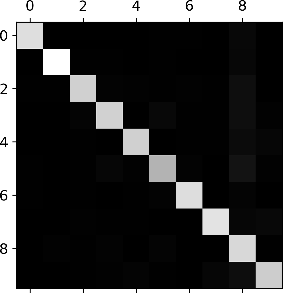
This confusion matrix looks fairly good, since most images are on the main diagonal, which means that they were classified correctly. The 5s look slightly darker than the other digits, which could mean that there are fewer images of 5s in the dataset or that the classifier does not perform as well on 5s as on other digits. In fact, you can verify that both are the case.

Let’s focus the plot on the errors. First, you need to divide each value in the confusion matrix by the number of images in the corresponding class, so you can compare error rates instead of absolute number of errors (which would make abundant classes look unfairly bad):

row_sums = conf_mx.sum(axis=1, keepdims=True)
norm_conf_mx = conf_mx / row_sums

Now let’s fill the diagonal with zeros to keep only the errors, and let’s plot the result:

np.fill_diagonal(norm_conf_mx, 0)
plt.matshow(norm_conf_mx, cmap=plt.cm.gray)
plt.show()

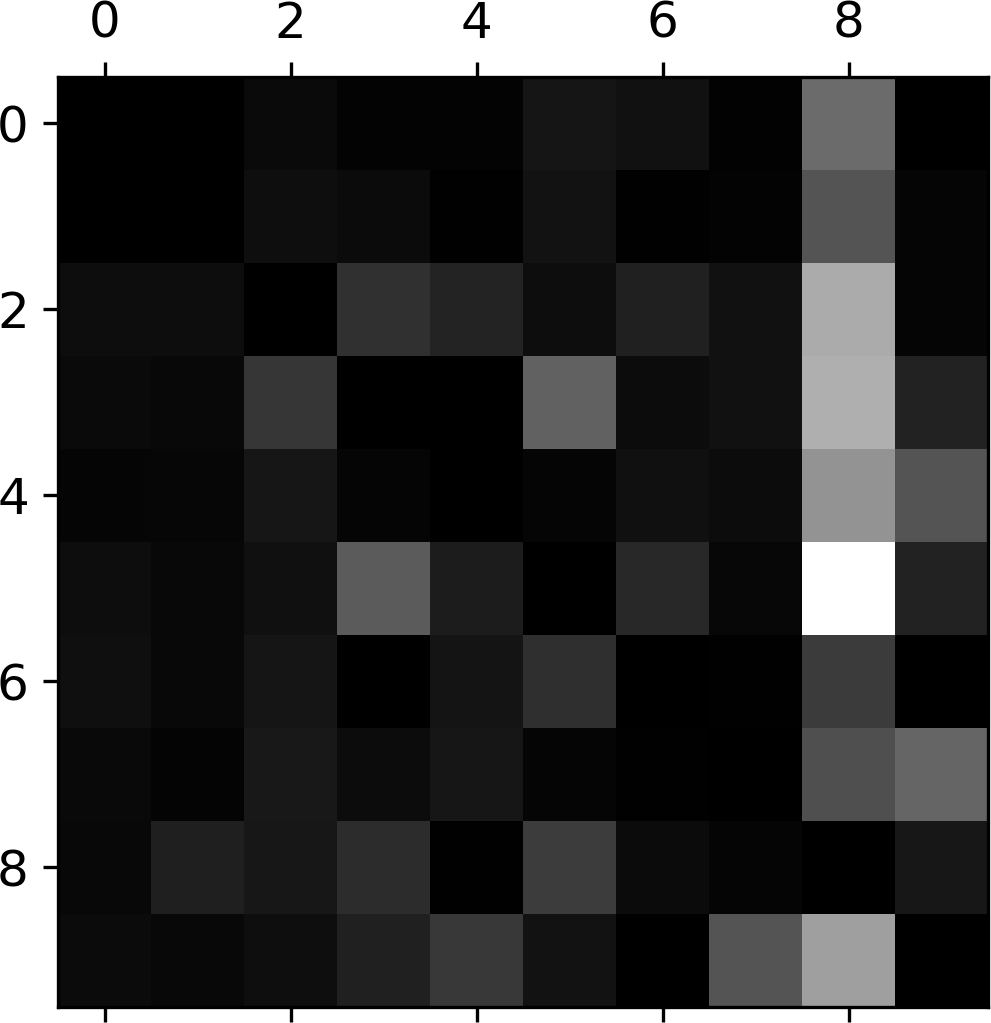
Now you can clearly see the kinds of errors the classifier makes. Remember that rows represent actual classes, while columns represent predicted classes. The column for class 8 is quite bright, which tells you that many images get misclassified as 8s. However, the row for class 8 is not that bad, telling you that actual 8s in general get properly classified as 8s. As you can see, the confusion matrix is not necessarily symmetrical. You can also see that 3s and 5s often get confused (in both directions).

Analyzing the confusion matrix can often give you insights on ways to improve your classifier. Looking at this plot, it seems that your efforts should be spent on reducing the false 8s. For example, you could try to gather more training data for digits that look like 8s (but are not) so the classifier can learn to distinguish them from real 8s. Or you could engineer new features that would help the classifier—for example, writing an algorithm to count the number of closed loops (e.g., 8 has two, 6 has one, 5 has none). Or you could preprocess the images (e.g., using Scikit-Image, Pillow, or OpenCV) to make some patterns stand out more, such as closed loops.

Analyzing individual errors can also be a good way to gain insights on what your classifier is doing and why it is failing, but it is more difficult and time-consuming. For example, let’s plot examples of 3s and 5s (the plot_digits() function just uses Matplotlib’s imshow() function; see this chapter’s Jupyter notebook for details):

cl_a, cl_b = 3, 5
X_aa = X_train[(y_train == cl_a) & (y_train_pred == cl_a)]
X_ab = X_train[(y_train == cl_a) & (y_train_pred == cl_b)]
X_ba = X_train[(y_train == cl_b) & (y_train_pred == cl_a)]
X_bb = X_train[(y_train == cl_b) & (y_train_pred == cl_b)]

plt.figure(figsize=(8,8))
plt.subplot(221); plot_digits(X_aa[:25], images_per_row=5)
plt.subplot(222); plot_digits(X_ab[:25], images_per_row=5)
plt.subplot(223); plot_digits(X_ba[:25], images_per_row=5)
plt.subplot(224); plot_digits(X_bb[:25], images_per_row=5)
plt.show()

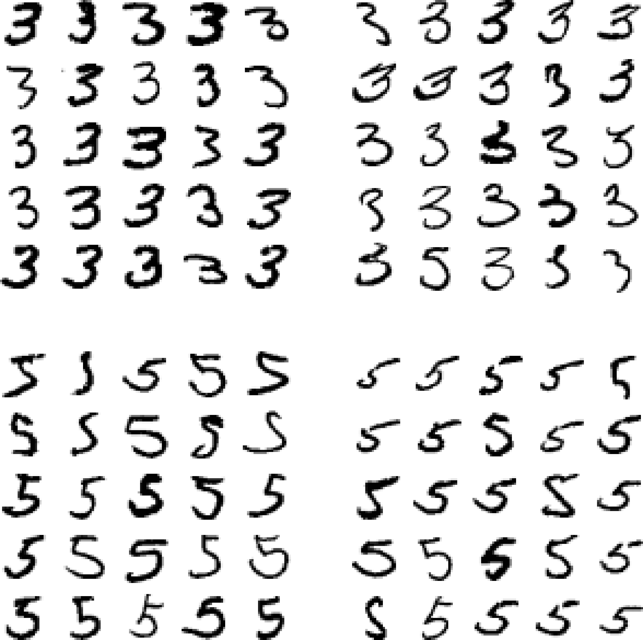
The two 5×5 blocks on the left show digits classified as 3s, and the two 5×5 blocks on the right show images classified as 5s. Some of the digits that the classifier gets wrong (i.e., in the bottom-left and top-right blocks) are so badly written that even a human would have trouble classifying them (e.g., the 5 on the 1^st row and 2^nd column truly looks like a badly written 3). However, most misclassified images seem like obvious errors to us, and it’s hard to understand why the classifier made the mistakes it did.³ The reason is that we used a simple SGDClassifier, which is a linear model. All it does is assign a weight per class to each pixel, and when it sees a new image it just sums up the weighted pixel intensities to get a score for each class. So since 3s and 5s differ only by a few pixels, this model will easily confuse them.

The main difference between 3s and 5s is the position of the small line that joins the top line to the bottom arc. If you draw a 3 with the junction slightly shifted to the left, the classifier might classify it as a 5, and vice versa. In other words, this classifier is quite sensitive to image shifting and rotation. So one way to reduce the 3/5 confusion would be to preprocess the images to ensure that they are well centered and not too rotated. This will probably help reduce other errors as well.

Multilabel Classification

Until now each instance has always been assigned to just one class. In some cases you may want your classifier to output multiple classes for each instance. For example, consider a face-recognition classifier: what should it do if it recognizes several people on the same picture? Of course it should attach one tag per person it recognizes. Say the classifier has been trained to recognize three faces, Alice, Bob, and Charlie; then when it is shown a picture of Alice and Charlie, it should output [1, 0, 1] (meaning “Alice yes, Bob no, Charlie yes”). Such a classification system that outputs multiple binary tags is called a multilabel classification system.

We won’t go into face recognition just yet, but let’s look at a simpler example, just for illustration purposes:

from sklearn.neighbors import KNeighborsClassifier

y_train_large = (y_train >= 7)
y_train_odd = (y_train % 2 == 1)
y_multilabel = np.c_[y_train_large, y_train_odd]

knn_clf = KNeighborsClassifier()
knn_clf.fit(X_train, y_multilabel)

This code creates a y_multilabel array containing two target labels for each digit image: the first indicates whether or not the digit is large (7, 8, or 9) and the second indicates whether or not it is odd. The next lines create a KNeighborsClassifier instance (which supports multilabel classification, but not all classifiers do) and we train it using the multiple targets array. Now you can make a prediction, and notice that it outputs two labels:

>>> knn_clf.predict([some_digit])
array([[False,  True]])

And it gets it right! The digit 5 is indeed not large (False) and odd (True).

There are many ways to evaluate a multilabel classifier, and selecting the right metric really depends on your project. For example, one approach is to measure the F₁ score for each individual label (or any other binary classifier metric discussed earlier), then simply compute the average score. This code computes the average F₁ score across all labels:

>>> y_train_knn_pred = cross_val_predict(knn_clf, X_train, y_multilabel, cv=3)
>>> f1_score(y_multilabel, y_train_knn_pred, average="macro")
0.976410265560605

This assumes that all labels are equally important, which may not be the case. In particular, if you have many more pictures of Alice than of Bob or Charlie, you may want to give more weight to the classifier’s score on pictures of Alice. One simple option is to give each label a weight equal to its support (i.e., the number of instances with that target label). To do this, simply set average="weighted" in the preceding code.⁴

Multioutput Classification

The last type of classification task we are going to discuss here is called multioutput-multiclass classification (or simply multioutput classification). It is simply a generalization of multilabel classification where each label can be multiclass (i.e., it can have more than two possible values).

To illustrate this, let’s build a system that removes noise from images. It will take as input a noisy digit image, and it will (hopefully) output a clean digit image, represented as an array of pixel intensities, just like the MNIST images. Notice that the classifier’s output is multilabel (one label per pixel) and each label can have multiple values (pixel intensity ranges from 0 to 255). It is thus an example of a multioutput classification system.

Let’s start by creating the training and test sets by taking the MNIST images and adding noise to their pixel intensities using NumPy’s randint() function. The target images will be the original images:

noise = np.random.randint(0, 100, (len(X_train), 784))
X_train_mod = X_train + noise
noise = np.random.randint(0, 100, (len(X_test), 784))
X_test_mod = X_test + noise
y_train_mod = X_train
y_test_mod = X_test

Let’s take a peek at an image from the test set (yes, we’re snooping on the test data, so you should be frowning right now):

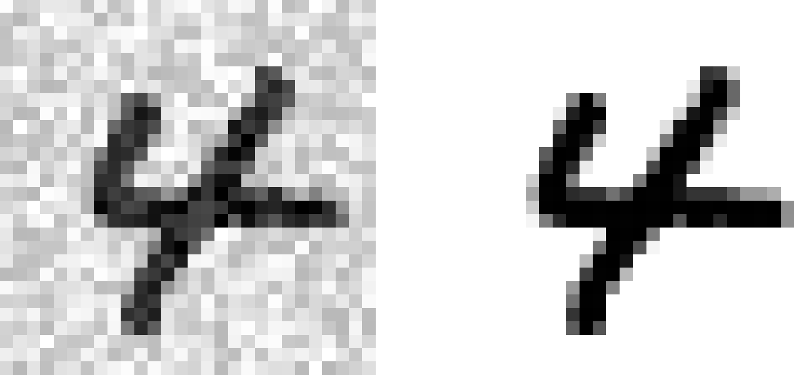
On the left is the noisy input image, and on the right is the clean target image. Now let’s train the classifier and make it clean this image:

knn_clf.fit(X_train_mod, y_train_mod)
clean_digit = knn_clf.predict([X_test_mod[some_index]])
plot_digit(clean_digit)

Looks close enough to the target! This concludes our tour of classification. Hopefully you should now know how to select good metrics for classification tasks, pick the appropriate precision/recall tradeoff, compare classifiers, and more generally build good classification systems for a variety of tasks.

Exercises

1. Try to build a classifier for the MNIST dataset that achieves over 97% accuracy on the test set. Hint: the KNeighborsClassifier works quite well for this task; you just need to find good hyperparameter values (try a grid search on the weights and n_neighbors hyperparameters).

2. Write a function that can shift an MNIST image in any direction (left, right, up, or down) by one pixel.⁵ Then, for each image in the training set, create four shifted copies (one per direction) and add them to the training set. Finally, train your best model on this expanded training set and measure its accuracy on the test set. You should observe that your model performs even better now! This technique of artificially growing the training set is called data augmentation or training set expansion.

3. Tackle the Titanic dataset. A great place to start is on Kaggle.

4. Build a spam classifier (a more challenging exercise):

   • Download examples of spam and ham from Apache SpamAssassin’s public datasets.

   • Unzip the datasets and familiarize yourself with the data format.

   • Split the datasets into a training set and a test set.

   • Write a data preparation pipeline to convert each email into a feature vector. Your preparation pipeline should transform an email into a (sparse) vector indicating the presence or absence of each possible word. For example, if all emails only ever contain four words, “Hello,” “how,” “are,” “you,” then the email “Hello you Hello Hello you” would be converted into a vector [1, 0, 0, 1] (meaning [“Hello” is present, “how” is absent, “are” is absent, “you” is present]), or [3, 0, 0, 2] if you prefer to count the number of occurrences of each word.

   • You may want to add hyperparameters to your preparation pipeline to control whether or not to strip off email headers, convert each email to lowercase, remove punctuation, replace all URLs with “URL,” replace all numbers with “NUMBER,” or even perform stemming (i.e., trim off word endings; there are Python libraries available to do this).

   • Then try out several classifiers and see if you can build a great spam classifier, with both high recall and high precision.

Solutions to these exercises are available in the online Jupyter notebooks at https://github.com/ageron/handson-ml2.