Table of Contents for

Practical Forensic Imaging

4
PLANNING AND PREPARATION

This chapter describes the preparatory steps performed prior to imaging a disk or storage medium. These include setting up an audit trail of investigator activity, saving output for reports, and deciding on naming conventions. In addition, I describe various logistical challenges involved in the forensic acquisition of storage media and how to establish a protected write-blocking environment.

The subject of forensic readiness overlaps somewhat with the sections in this chapter. However, forensic readiness is a broader topic that includes general planning, budgeting, lab infrastructure, staff training, hardware and software purchasing, and so on. If you consider the preceding requirements needed as “macro” forensic readiness, you can consider the information in this chapter as “micro” forensic readiness. The focus is narrower and includes setting up a forensic examiner’s workstation environment and the tools and individual tasks needed to analyze a disk or storage media.

It is worth noting that forensic readiness in a private sector organization (in a corporate forensic lab, for example) is different from forensic readiness in some public sector organizations, such as law enforcement agencies. Private sector organizations, especially large corporate IT environments, can dictate how their IT infrastructure is built and operated. Forensic readiness in this controlled environment can be built into the IT infrastructure, providing advantages for a forensic examiner in the event of an investigation or incident. This chapter focuses on preparatory forensic tasks, which the private sector and public sector have in common.

Maintain an Audit Trail

An audit trail or log maintains a historical record of actions, events, and tasks. It can have various levels of detail and can be either manual or automated. This section covers several command line methods for manually tracking tasks as well as automated logging of command line activity.

Task Management

During a forensic examination, it’s beneficial to keep a high-level log of pending and completed activity. Pending tasks turn into completed tasks, and completed tasks make up the examination’s historical record. Often while working, you’ll think of a task that you need to address sometime in the future or a task you’ve completed and should note. Making quick notes and more comprehensive task lists becomes increasingly valuable as the length of the examination grows (possibly to many hours, days, or longer) or when more than one examiner is involved.

Maintaining a list of pending and completed tasks during an examination is important for a number of reasons:

• Helps ensure nothing was forgotten

• Avoids duplicating work already done

• Improves collaboration and coordination when working in teams

• Shows compliance with policies and procedures

• Facilitates accounting, including billing

• Helps produce documentation and reports (formal incident reports or forensic reports)

• Allows for post-incident review to identify lessons learned and support process optimization

• Helps to maintain a longer-term historical record of completed activity

• Supports learning and education for new team members

• Serves as a guide to remember complex procedures

• Provides information for troubleshooting problems and getting support

• Maintains a record of work done by external and third-party examiners

Many commercial task managers and investigation management tools are available, but the focus in this section is on simple task management that you can do from the command line. Using the command line permits you to quickly track tasks and activity without leaving the terminal to access some other graphical or web-based application.

Many open source command line task managers are available and can be used to manage a forensic examiner’s activity. The most important criteria include reliable task recording and a detailed timestamp (not just dates).

Taskwarrior

Taskwarrior is a popular task manager with many features for managing large task lists in a quick and efficient manner. You’ll find more information about Taskwarrior at http://taskwarrior.org/. The following examples show Taskwarrior commands in practical use in a forensic lab context.

To add several pending tasks:

$ task add acquire PC disk and transfer to evidence safe due:friday
Created task 1.
$ task add have a meeting with investigation team to plan analysis
Created task 2.

To list the current task list (task info will show times and more detailed information):

$ task list

ID Due        Age Description
 1 2015-06-05 1m  acquire PC disk and transfer to evidence safe
 2            3s  have a meeting with investigation team to plan analysis

2 tasks

To complete a task on the task list:

$ task 2 done
Completed task 2 'have a meeting with investigation team to plan analysis'.
Completed 1 task.

To log a completed task without placing it on the task list:

$ task log requested history of PC use at the firm
Logged task.

Taskwarrior is useful for managing large numbers of tasks. It provides reports, searching, sorting, and various levels of customizable detail. Taskwarrior maintains timestamps and unique identifiers (UUID) for each task, manages prioritization of pending tasks, and keeps a history of completed tasks. The ability to create user-defined attributes makes it customizable for specific settings, such as a forensics lab or examination process.

Todo.txt

You can also maintain a list of completed tasks and pending work by editing a simple text file. An example is the todo.txt file format by Gina Trapani (see http://todotxt.com/ for more information). The todo.txt system defines a file format for task creation and completion dates, priorities, projects, and contexts. It also provides a shell script to manage the todo.txt file. Although the todo.sh script performs all the necessary operations on the todo.txt task list, the file format can be managed using a regular text editor. The notation indicates priority with parentheses ((A), (B), and so on), context keywords with @, and project keywords with +. Completed tasks are prefixed with an x. Here is an example todo.txt file:

(A) Sign chain of custody forms @reception
(B) Start forensic acquisition +Disk_A @imagingstation
Discuss analysis approach with investigation team @meetingroom
x 2015-05-30 08:45 upgrade ram in imaging PC @imagingstation

The todo.txt apps don’t use timestamps, only dates. If you use this system, you must manually include the time with the completed task.

Shell Alias

You can also maintain an examiner activity log of completed tasks without the use of task management software. For example, here is a simple shell alias that redirects a short description into a file with a timestamp:

$ alias log="echo $2 \`date +%FT%R\` >> ~/examiner.log"

You can customize the log filename and date format as desired. Making a quick note of activity or viewing past activity takes a simple one-line command, which you can enter anytime during the examination process. When something significant or notable occurs, enter log followed by the short description of the action taken. For example:

$ log removed hdd from PC and attached to examiner machine
...
$ log started forensic acquisition of the disk
...
$ log acquisition completed, disk sealed in evidence bag
...
$ cat ~/examiner.log
2015-05-30T09:14 informed that seized PC was enroute to forensic lab
2015-05-30T10:25 PC arrived, chain of custody forms signed
2015-05-30T10:47 removed hdd from PC and attached to examiner machine
2015-05-30T10:55 started forensic acquisition of the disk
2015-05-30T15:17 acquisition completed, disk sealed in evidence bag
2015-05-30T16:09 disk transferred to evidence safe for storage

Simple systems for managing tasks are useful for staff who spend much of their time working on the command line. They are also advantageous for remotely working on systems with secure shell (ssh).

Shell History

This section discusses how to set up automated logging of shell commands entered by the examiner on the command line. Ideally, this command logging should not increase complexity or interfere with the forensic work in progress. Using various tools, you can log the examiner’s command line activity with automated background processes. This approach is completely transparent to the examiner during the course of a forensic investigation.

The Unix/Linux shell was not originally designed with logging or audit trails in mind. In the past, patches have been created to augment the history mechanism, hacks have attempted to capture commands as the shell is used, and commercial products have performed various enterprise logging. Developing a robust auditing and compliance system to log all commands with timestamps, including shell builtins as well as executed programs and pipelines, is beyond the scope of this book.

The Bash shell history can be configured to satisfy the following basic requirements:

• Record the command entered by the examiner

• Record a timestamp for each command entered

• Record all commands, including duplicates, comments, and space-prefixed commands

• Avoid truncating or overwriting history files

• Avoid conflicts when using multiple terminal windows on the same system

• Include root and non-root command history

Using basic Bash shell history as an audit trail is rudimentary. Important information, such as the command completion time, the working directory where the command was executed, and the return code, are not logged. The Bash history is also not a tamper-resistant system: the examiner can easily modify or delete the history. Creating a secure and tamper-resistant audit environment with restricted access is beyond the scope of this book.

Some shells, such as zsh, have additional history features that allow for the logging of elapsed time. Other proposed solutions to improve shell logging include the use of PS1, PROMPT_COMMAND, trap and DEBUG, and key bindings to modify a command before executing. Using sudo logging; auditd logging; or special scripts, such as preexec.sh, can also increase command line logging. A useful tutorial at http://www.pointsoftware.ch/en/howto-bash-audit-command-logger/ discusses this problem at length and proposes a solution. The command line audit trail should be tailored to particular lab policies or expectations.

For basic shell command logging, the built-in shell history functionality can be configured to record command line activity. Bash provides some useful functionality, including the ability to enable the time stamping of the commands entered. You can add the following commands to the Linux startup scripts (.bashrc and so on) to enable the basic requirements outlined in the previous list:

set -o history
shopt -s histappend
export HISTCONTROL=
export HISTIGNORE=
export HISTFILE=~/.bash_history
export HISTFILESIZE=-1
export HISTSIZE=-1
export HISTTIMEFORMAT="%F-%R "

These commands ensure that history is enabled and in append mode (as opposed to overwriting with each new login). The two variables HISTCONTROL and HISTIGNORE control which commands are saved to the history file. A common default setting is to ignore duplicates and commands beginning with a space. To ensure complete logging of all commands, the HISTCONTROL and HISTIGNORE variables are explicitly set to null. The HISTFILE variable is explicitly set to ensure command history held in memory is saved when a shell exits. HISTFILESIZE and HISTSIZE are set to -1 to ensure history is not truncated or overwritten. The HISTTIMEFORMAT variable enables timestamps to be written to the history file and allows you to set a time format. The format can include regional settings and should include a timestamp, not just the date.

At the end of the examination, the history can be saved to a text file and included in the examination’s supporting data files. The history can then be reset and made ready for the next examination by using the following commands:

$ history > examiner_bash_history.txt
$ history -c; history -w

Synchronizing the history across multiple shell instances can be tricky because each shell keeps its history in memory and writes it to the history file only on exit. Setting the variable PROMPT_COMMAND='history -a; history -r' will write (append) and read new commands from the Bash history file every time the command prompt is displayed.

A command logger that is actively developed is Snoopy: it provides a number of features, including logging the commands to syslog. Snoopy is a preloaded library that functions as a wrapper around the execv() and execve() system calls. It is transparent to users, and you can enable and configure it by adding the Snoopy library to /etc/ld.so.preload and editing the /etc/snoopy.ini file. For example, suppose the following series of commands are entered on the Bash command prompt:

# fls -p -r /dev/sda1 | grep -i "\.doc$" |wc -l
10

These commands are individually logged to syslog with various details:

Jun  5 10:47:05 lab-pc snoopy[1521]: [uid:0 sid:1256 tty:(none) cwd:/ filename:
    /bin/grep]: grep -i \.doc$
Jun  5 10:47:05 lab-pc snoopy[1522]: [uid:0 sid:1256 tty:(none) cwd:/ filename:
    /usr/bin/wc]: wc -l
Jun  5 10:47:05 lab-pc snoopy[1520]: [uid:0 sid:1256 tty:/dev/pts/0 cwd:/ filename:
    /usr/bin/fls]: fls -p -r /dev/sda1

You’ll find more information and the latest release of Snoopy at https://github.com/a2o/snoopy/.

Terminal Recorders

In some cases, it might be useful to show the work done in the terminal, complete with command output (stdout), error messages (stderr), and other messages or activity visible in a terminal session. Several tools exist to capture session activity and even provide playback of the session.

The most well-known tool is script. In this example, script is started and the output appended to a file together with timing data for replay. After running script, you can execute any normal shell commands, and they’ll be saved for later viewing.

$ script -a -tscript.timing script.output
Script started, file is script.output

When the recorded session is finished, enter exit or press CTRL-D. You can view the recording using the scriptreplay command as follows:

$ scriptreplay -m1 -tscript.timing script.output
...[session plays back here]...

Common issues that make this method challenging are the handling of control characters and events such as terminal resizing. Other TTY recorders and sniffers, such as ttyrec and termrec, are available with similar functionality and features.

Terminal multiplexers, such as tmux and GNU screen, also provide some level of logging that can be useful in certain situations. With screen, you can set up logging for a detached session from within a session (CTRL-A followed by H). The tmux terminal multiplexer now supports logging by using the pipe-pane option, as shown here:

$ tmux pipe-pane -o -t session_index:window_index.pane_index 'cat >> ~/output
    .window_index-pane_index.txt'

Linux Auditing

Professional labs might want to implement more robust logging or an audit trail to satisfy stricter organizational policies or regulatory requirements. One possibility to achieve this is through auditd, a Linux audit package. Typically, this involves running the auditd daemon with pam_tty_audit.so configured as a pam module. You can review audit trail activity using the aureport command.

Using auditd provides several security advantages, especially when used with granular access control, such as sudo. Audit trails, in particular those logging to a central log host, can be made relatively tamper resistant, ensuring an increased level of integrity when recording examination work.

Comprehensive audit trails can record all TTY activity (including keystrokes), as well as monitor file access and many other events on a system. Setting up auditing and audit reporting can be a complex process, one beyond the scope of this book.

You’ll find discussions of other solutions and hacks in various places, including http://www.pointsoftware.ch/en/howto-bash-audit-command-logger/ and http://whmcr.com/2011/10/14/auditd-logging-all-commands/.

As of Bash version 4.1, a new feature allowing command history logging to syslog has been added (it may require recompilation to enable).

Organize Collected Evidence and Command Output

When conducting a forensic examination on the command line, it’s common to save command output from various tools and utilities to files for future reference and reporting. You can do this by redirecting the output of commands to text files. Those files can be saved with the rest of the examination data collected. During the process of collecting and saving large amounts of evidence data, it is important to keep your file and directory structure organized and understandable. This section talks about various strategies to achieve this goal.

Naming Conventions for Files and Directories

To reduce confusion among all the files, directories, mount points, images, and other saved data collected during an examination, it’s best to follow a naming convention. Make it descriptive enough to be intuitive, but avoid redundancy in the wording and file extensions. Most important, make naming conventions consistent throughout an investigation or incident and across multiple incidents.

Certain unique identifiers are associated with systems, storage media devices, and removable media. Such identifiers can be useful when deciding on a naming convention:

• Company asset tag or inventory number for PCs

• Manufacturer serial number for disk drives

• 64-bit World Wide Name (WWN) for disk drives

• Block device UUID for filesystems and RAIDs

• Forensic hash value for disk drive images

• 48-bit MAC address for network interface cards (NICs)

• Forensic lab evidence number (possibly a sticker or tag on the drive)

• Forensic lab evidence bag number (evidence bag containing the disc)

Wherever sensible, start all numbering with 1, not 0. Programmers and engineers have a tendency to start at 0, but people who read and review the examination reports may not have a technical background (lawyers, judges, managers, and so on) and expect numbering to start with 1.

Raw image files use the extension *.raw throughout this book. The commonly used *.dd extension implies that a dd tool was used, which might not be the case. The *.raw extension describes the file accurately without associating it with the particular tool used to acquire the image.

Ideally, a raw image’s filename should link a forensic image to a unique attribute of the physical object. If a forensic format is used, this unique information can be embedded as metadata in the forensic image file. This allows you to associate a lone physical disk with an image and associate a lone image with a physical disk. The disk and the image then remain linked without any dependencies on surrounding context (directory names, evidence shelves, and so on). This establishes a chain of custody link between the physical and digital worlds.

If large numbers of disks are under analysis, possibly include a serial number in the image filename. You can include varying levels of detail in a filename. Although the filename server12-slot3-seagate-3.5in-disk-500gb -SN12345ACBDEE.raw is very descriptive, it might be too detailed and cumbersome to work with. A practical naming convention for many basic incidents could simply be the storage media type with a number, for example, disk1, tape1, ssd1, stick1, card1, cdrom1, dvd1, bluray1, floppy1, and so on. In some cases, using a short description of the disk and the serial number might be the most suitable approach, for example, crucial-ssd -15030E69A241.raw. Often, it’s helpful to create image names that exam-iners can easily discuss in conversation, such as, “We found the file on disk1.” Terms used in conversations, raw examination output, and final reports should have a consistent nomenclature.

When you’re extracting files from disk images, archive files, or other compound images, add an underscore to the filename to indicate it has been extracted. This will prevent you and others from accidentally opening malware, HTML pages with tracking bugs, macros in Office documents, or other executables and scripts that might execute on opening. Some examples are shown here:

$ icat image.raw 68 > photo.jpg_
$ icat image.raw 34 > customerlist.xls_
$ icat image.raw 267 > super-updater57.exe_

If an extracted file already ends with an underscore, add another one. An appended underscore make it obvious that a file has been extracted as evidence from a suspect drive.

When you’re analyzing an extracted file, saving tool output, or making manual notes, create a text file with the original name and append _.txt to it. For example:

$ exif photo.jpg_ > photo.jpg_.txt
$ vi customerlist.xls_.txt
$ objdump -x super-updater57.exe_ > super-updater57.exe_.txt

The _.txt extension signifies that the text file contains notes, tool output, and results of forensic analysis work about the extracted file. The filename is associated with the file originally extracted from the image. The text file may contain bookmarks and examiner annotations that can be searched. Unless it’s otherwise clear where an extracted file came from (which disk, partition, and so on), it’s good practice to have such corresponding text files; they can also indicate why it was chosen for extraction.

A file extension should always indicate the format of the content. For example:

• *.txt can be opened and read using a text editor.

• *.raw is a raw data dump (disk, memory, and so on).

• *.pcap is captured network traffic.

• *.db is a database (possibly a Sleuth Kit file list).

• *.sfs is a SquashFS evidence container.

• *.e01 and *.aff are forensic formats.

Each case, incident, or investigation will have an associated physical storage media. Storage media will have a corresponding forensic image and associated output from various programs (hdparm, smartctl, and so on). Each forensic image will have associated output from various programs (mmls, fls, and so on), and each extracted file may have associated output from various programs (exif, objdump, and so on). A naming convention will help keep everything organized and allow the organizing system to scale as the investigation data grows.

How much information should be embedded into filenames and directory names? When is it more sensible to have a corresponding description text file with additional information? How should the corresponding file be associated with an image? Consider the following examples of two representations of the same incident.

An example of information embedded into filenames looks like this:

case42.txt
image6.case42.raw
image6.case42.raw.txt
mmls.image6.case42.txt
fls.part1.image6.case42.txt

An example of that same information embedded into a directory structure looks like this:

./case42/case.txt
./case42/image6/image.raw
./case42/image6/image.raw.txt
./case42/image6/mmls.txt
./case42/image6/part1/fls.txt

For manually written notes, further descriptions, caveats, issues, and other random comments within a certain context, storing the information in simple notes.txt or readme.txt files within working directories can be useful. They can provide reminders, hints, or warnings for you or other examiners to read at a later date.

When you’re noting web URLs that might pose a risk if opened, replace http with hxxp to prevent others from accidentally clicking them. Such links might take the user to malware, personal sites monitored by a suspect, sites with tracking bugs, or other content that should not be accessed without understanding the consequences.

Scalable Examination Directory Structure

Each incident, case, or investigation should have a single unique directory (for example, case42). All collected evidence, images, and analysis work should be contained within a hierarchy under that one root directory. As investigations scale, a well-planned directory structure can scale with it. Having a single directory is also practical when multiple forensic examiners are working on the same incident and sharing the directory structure. Be prepared to reorganize the directory structure if an incident grows in complexity. If a large number of files are being extracted for individual analysis, consider having an export directory (similar to EnCase).

Examinations often scale unexpectedly, and a forensic examination that starts with a single disk under suspicion might expand into a larger examination involving multiple PCs with many disks. For example, suppose someone reports strange or suspicious behavior of a PC or employee. A single disk is seized for examination. Preliminary examination results find a USB stick is also involved. It is found and examined, and a second PC is linked to the incident. That PC has two internal hard disks and DVD burner. Further search reveals a box of DVDs full of data hidden in a closet. Then it turns out that an external USB hard disk and a spare notebook in another building are also involved in the incident. The collected evidence has grown from a single hard disk to 16 storage media items. This hypothetical incident is not uncommon in large organizations. When preparing for an examination, expanded coverage should be anticipated. The naming convention should be designed to scale as the size of an investigation grows.

Some PCs are used by multiple people, and some people use multiple PCs. Notebooks are not necessarily bound to a physical location. Removable media can be shared and attached to multiple PCs and notebooks. Over long periods of time, PC hardware will change, offices may change, departments will experience staff turnover, and organizational restructuring may occur. Be sure to design file and directory names to accommodate these changes.

As an examination progresses, the number of output files will grow as more collected data is analyzed and output is produced. A good practice is to create a directory structure to separate the files and organize the output of the examination. As with filenames, the directory name should indicate the contents without revealing confidential information. Creating a separate directory for each disk or image analyzed segregates files and allows an investigation to scale up.

The smallest examination usually consists of a single disk. A slightly larger examination might consist of a PC containing multiple disks; consider the following example directory structure:

As another example, consider the examination of an entire workplace that consists of a desktop PC (possibly with multiple disks), a notebook, several USB drives, multiple CD-ROMs and DVDs, and an external disk pack. A convenient directory structure would organize each piece of storage media where the command output files are stored, allowing an examination to easily scale further. Consider a larger investigation consisting of multiple workplaces, across multiple office buildings, spread out across multiple countries. In large global organizations, such investigations can occur; therefore, having a well-thought-out naming convention will maintain the organization of the examination process.

It’s advantageous to rely on a directory structure to separate command output from different disks, PCs, users, and locations. As a result, you won’t need to embed this information into the output filenames. For example:

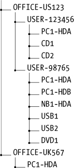
In this example, two office locations are US123 and UK567, in the United States and the United Kingdom, respectively. The US office is divided by user workplaces, and a directory is used for each piece of storage media under examination. The UK office PC is not associated with any particular user (possibly located in a meeting room), and this is reflected in the directory structure.

Instead of using an employee identifier for the storage media, an organization’s IT inventory number can be used for the storage media in the directory structure. This unique identifier will likely have additional information associated with it (date of purchase, department, office location, user details, software installed, history of use, and so on). Confidentiality reasons might require you to omit information from the filenames and directory structure. For example, names of suspected or targeted individuals should not be embedded into filenames. Rather, you should use an identifier, initials, or an employee number. Code names for investigations might also be used. They provide a minimal level of protection if the information is lost, stolen, or otherwise accessed at a later date.

Save Command Output with Redirection

After creating the directory structure to store the analysis results from various items under examination, typical shell command output is redirected into files from stdout as shown here:

# fls /dev/sda1 > fls-part1.txt
# fls /dev/sda2 > fls-part2.txt

To include regular output and error messages, you need to redirect stdout and stderr file descriptors to the file. Newer versions of Bash provide an easy-to-remember method by adding an ampersand to the redirection (this also applies when piping to another program):

# fls /dev/sda &> fls-part1.txt

Other shells and earlier Bash versions might require 2>&1 notation for combining stderr and stdin. For example:

# fls /dev/sda > fls-part1.txt 2>&1

When a text file already exists and you need to add additional information to it, you can use the >> notation to specify an append operation. For example:

# grep clientnames.xls fls-part1.txt >> notes.txt

Here, all instances of a known filename are added to the end of the notes.txt file.¹ If notes.txt doesn’t exist, it will be created.

Many forensic tasks performed on the command line are time-consuming and may take many hours to complete (disk imaging, performing operations on very large files, and so on). Having a timestamp indicating the duration of the command can be useful. The time command provides this functionality. There are two common implementations of the time command: one is a shell builtin with rudimentary features, and the other is a GNU utility with additional features. The primary advantage of the shell builtin time version is that it will time an entire pipeline of commands, whereas GNU time will only time the first command in a pipeline.

Here is an example of using the time command to run a disk-imaging program:

# time dcfldd if=/dev/sdc of=./ssd-image.raw
3907328 blocks (122104Mb) written.
3907338+1 records in
3907338+1 records out

real    28m5.176s
user    0m11.652s
sys     2m23.652s

The zsh shell can log the elapsed time of a command as part of the history file. This functionality is currently not available in Bash.

Another useful command for some situations is the timestamp output command ts. Any output piped into ts will have a timestamp appended to each line of output.

# (ls -l image.raw; cp -v image.raw /exam/image.raw; md5sum /exam/image.raw) |ts
May 15 07:45:28 -rw-r----- 1 root root 7918845952 May 15 07:40 image.raw
May 15 07:45:40 'image.raw' -> '/exam/image.raw'
May 15 07:45:53 4f12fa07601d02e7ae78c2d687403c7c  /exam/image.raw

In this example, three commands were executed (grouped together with parentheses) and the command outputs were sent to ts, creating a timeline.

Assess Acquisition Infrastructure Logistics

Various logistical issues are important when performing forensic acquisition of storage media. Managing large acquired forensic images is not a trivial task and so requires planning and forethought. Factors such as disk capacity, time duration, performance, and environmental issues need to be considered.

Image Sizes and Disk Space Requirements

Forensic images of storage media are orders of magnitude larger than the small file sizes a PC typically handles. Managing disk image files of this size takes additional thought and planning. You also need to consider certain logistical factors when you’re preparing an examination system. Careful preparation and planning for an examination will save you time and effort, as well as help you avoid problems that might disrupt the process.

When creating a forensic image of a disk (hundreds of gigabytes or tera-bytes), it is not files that are copied, but the individual disk sectors. If a 1TB disk has only a single 20K Microsoft Word document on it, an uncompressed forensic image will still be 1TB. As of this writing, 10TB disks are now on the market, increasing the challenge for performing forensic acquisition.

When managing disk images, the examiner’s time and the examiner host’s disk capacity are the main logistical factors that need to be considered. Before beginning a forensic acquisition of a subject disk or storage media, you need to ask a number of questions:

• Can the attached storage be analyzed in place without taking a forensic image?

• What is the size of the subject disk?

• What is the available space on the examiner’s machine?

• What is the potential for image compression?

• How much space do forensic tools need for processing and temporary files?

• What is the estimated number of files to be extracted for further analysis?

• How much memory and swap space is available on the examiner’s machine?

• Is there a possibility of more subject disks being added to the same case or incident?

• Is there an expectation to separately extract all slack or unallocated disk space?

• Are there plans to extract individual partitions (possibly including swap)?

• Is there a potential need to convert from one forensic format to another?

• Do disk images need to be prepared for transport to another location?

• Do subject disks contain virtual machine images to separately extract and analyze?

• Do subject disks contain large numbers of compressed and archive files?

• Are subject disks using full-disk encryption?

• Is there a need to burn images to another disk or DVDs for storage or transport?

• Is there a need to carve files from a damaged or partially overwritten filesystem?

• How are backups of the examiner host performed?

In some situations, it may not be necessary to image a disk. When certain triage or cursory searching is conducted, it may be enough to attach the disk to an examiner host and operate on the live subject disk. Depending on the triage or search findings, you can decide whether or not to take a forensic image. In a corporate environment, this approach could translate into downtime for an employee, because they must wait for a seized disk to be reviewed or analyzed. Corporate environments typically have a standard end-user PC build, which is designed without local user data (all data is saved to servers or clouds). It could be more economical simply to swap the original disk with a new disk. End-user PC disks are cheap, and replacing a subject disk with a new one could be a cost-saving alternative when factoring in the cost of employee downtime and the time needed to image a disk in the field.

File Compression

Using compression solves a number of the capacity challenges faced by a forensic examiner. You can use a compressed forensic format to store the resulting acquired image, but the effectiveness depends on a number of factors.

The compression algorithms you choose will have some effect on the size and time needed to compress a subject disk. A better compression ratio will take more time to compress (and subsequently uncompress).

A relatively new PC disk that contains a large number of untouched disk sectors (original manufacturer’s zeroed contents) will compress better than an older disk containing significant amounts of residual data in the unallocated sectors.

Disks that contain large amounts of compressed files (*.mp3, *.avi, and so on) will not compress much further, and as a result, forensic imaging tools will benefit less from added compression.

Encrypted subject disks or disks with large numbers of encrypted files will not compress as well as unencrypted content due to the data’s higher entropy level.

Sparse Files

Sparse files are worth mentioning because they have some advantages; however, they can also be problematic when calculating disk capacity. Some filesystems use metadata to represent a sequence of zeros in a file instead of actually writing all the zeros to the disk. Sparse files contain “holes” where a sequence of zeros is known to exist. To illustrate, a new drive containing mostly zeroed sectors is acquired with GNU dd,² first as a regular raw file and then as a sparse file.

# dd if=/dev/sde of=image.raw
15466496+0 records in
15466496+0 records out
7918845952 bytes (7.9 GB, 7.4 GiB) copied, 112.315 s, 70.5 MB/s

# dd if=/dev/sde of=sparse-image.raw conv=sparse
15466496+0 records in
15466496+0 records out
7918845952 bytes (7.9 GB, 7.4 GiB) copied, 106.622 s, 74.3 MB/s

The GNU dd command provides a conv=sparse flag that creates a sparse destination file. In these dd examples, you can see the number of blocks transferred is the same for both the normal and sparse files. In the following output, the file size and the MD5 hash are also identical. However, notice how the block size used on the filesystem is very different (7733252 blocks versus 2600 blocks):

# ls -ls image.raw sparse-image.raw
7733252 -rw-r----- 1 root root 7918845952 May 15 08:28 image.raw
   2600 -rw-r----- 1 root root 7918845952 May 15 08:30 sparse-image.raw

# md5sum image.raw sparse-image.raw
325383b1b51754def26c2c29bcd049ae  image.raw
325383b1b51754def26c2c29bcd049ae  sparse-image.raw

Although the sparse file requires much less space, the full byte size is still reported as the file size. This can cause confusion when calculating the real available disk capacity. Sparse files are often used by VM images and can become an issue when extracted for analysis.

You can also use sparse files as a method of compacting image files, but using compressed forensic formats or SquashFS containers is preferred and recommended. Not all programs and utilities can handle sparse files correctly, and the files can become problematic when moved between filesystems and platforms. Some programs may even expand sparse files when reading them.

Reported File and Image Sizes

Reporting data sizes is an important concept to grasp. When you’re working with forensic tools, size can refer to bytes, disk sectors, filesystem blocks, or other units of measurement. The notation for bytes can be prefixed with a multiplier (such as kilobytes, megabytes, gigabytes, terabytes, and so on), and the multiplier can refer to multiples of either 1000 or 1024. Disk sectors could represent sector sizes of either 512 bytes or 4096 bytes. The filesystem block size depends on the type of filesystem and the parameters used during creation. When you’re documenting sizes in a forensic context, it’s important to always include descriptive units.

Many Linux tools support the -h flag to report file sizes in a human readable form. For example, you can use ls -lh, df -h, and du -h to more easily view the size of files and partitions. An example ls output with several file sizes is shown here:

# ls -l
total 4
-rw-r----- 1 root root 2621440000 Jan 29 14:44 big.file
-rw-r----- 1 root root  104857600 Jan 29 14:41 medium.file
-rw-r----- 1 root root      51200 Jan 29 14:42 small.file
-rw-r----- 1 root root         56 Jan 29 14:44 tiny.file
# ls -lh
total 4.0K
-rw-r----- 1 root root 2.5G Jan 29 14:44 big.file
-rw-r----- 1 root root 100M Jan 29 14:41 medium.file
-rw-r----- 1 root root  50K Jan 29 14:42 small.file
-rw-r----- 1 root root   56 Jan 29 14:44 tiny.file

The sizes in the second command’s output are much easier to read and understand.

Moving and Copying Forensic Images

Moving and copying forensic disk images from one place to another requires planning and foresight. Don’t think of image files in the same way as typical end-user files (even though technically they’re the same).

Acquiring, copying, and moving large disk images may take many hours or even days depending on the size and speed of the source disk and other performance factors. Consider the following list of typical file and disk image sizes and the average amount of time needed to copy the file from one disk to another disk:³

• 5KB simple ASCII text email: less than 1 second

• 5MB typical MP3 music file: less than 1 second

• 650MB CD ISO image: about 5 seconds

• 5–6GB typical DVD or iTunes movie download: about 1 minute

• 64GB common mobile phone image: about 10 minutes

• 250GB common notebook disk image: 30-40 minutes

• 1TB typical desktop PC image: more than 2 hours

• 2TB typical external USB disk image: more than 4 hours

• 8TB internal disk image: more than 16 hours

Once a copy or move process has been started, disrupting it could leave the data in an incomplete state or require additional time to revert to the original state. A copy or move operation could create temporary files or result in two copies of the images existing temporarily.

In general, think carefully beforehand about the copying and moving of large data sets, and don’t interrupt the process once it has started.

Estimate Task Completion Times

The forensic acquisition process takes time to complete. During this time, people and other processes may be waiting. Therefore, it’s important to calculate and estimate the completion time needed for various processes. Also, determine whether you need to report estimated completion times to other parties, such as management, legal teams, law enforcement, or other investigators. It is important to manage expectations with regard to the time needed for completion.

Some important questions to consider include:

• Can the acquisition be safely left running overnight while nobody is around?

• Is the examiner machine unusable during the acquisition process (for performance reasons or other reasons)?

• Can other examination work be done while the forensic image is being acquired?

• When can several tasks be completed in parallel?

• Are there certain tasks or processes that can only be done sequentially?

• Are there tasks that will block other tasks until they’re completed?

• Can the workload be shared, delegated, or distributed across multiple examiners?

You can calculate an estimated completion time for an acquisition. From previous work and processes, you should know the approximate initial setup time. This includes factors such as completing paperwork, creating necessary directory structure, documenting the hardware, attaching suspect drives to the examiner host, deciding on the approach for acquisition, and so on. This will give you a time estimate for the preacquisition phase.

You can calculate the expected storage media acquisition time based on the amount of data (known) passing through the slowest component in the system (the bottleneck).

Performance and Bottlenecks

To improve the efficiency of a forensic acquisition, you can optimally tune the examiner host and assess the bottlenecks.

A performance bottleneck always occurs; this is simply the slowest component in the system, which all other components must wait for. In a forensic setting, the bottleneck should ideally be the subject disk. This is the evidence source and is the only performance variable that you can’t (or shouldn’t) modify.

You can assess the performance of various system components by reading the vendor specifications, querying the system with various tools, or running various benchmarking and measurement tests.

Useful tools to check the speed of various components include dmidecode, lshw, hdparm, and lsusb. Several command line examples are shown here.

To check the CPU family and model, current and maximum speed, number of cores and threads, and other flags and characteristics, use this command:

# dmidecode -t processor

Here is a command to view the CPU’s cache (L1, L2, and L3):

# dmidecode -t cache

To view the memory, including slots used, size, data width, speed, and other details, use this command:

# dmidecode -t memory

Here is a command to view the number of PCI slots, usage, designation, and type:

# dmidecode -t slot

A command to view the storage interfaces, type (SATA, NVME, SCSI, and so on), and speed:

# lshw -class storage

To view the speed, interface, cache, rotation, and other information about the attached disks (using device /dev/sda in this example), use this:

# hdparm -I /dev/sda

To view the speed of the external USB interfaces (and possibly an attached write blocker), use this command:

# lsusb -v

Reading the vendor documentation and querying a system will identify the speeds of various components. To get an accurate measurement, it’s best to use tools for hardware benchmarking and software profiling. Some tools for benchmarking include mbw for memory and bonnie++ for disk I/O.

The health and tuning of the OS is also a performance factor. Monitoring the logs (syslog, dmesg) of the examiner hardware can reveal error messages, misconfiguration, and other inefficiency indicators. Tools to monitor the performance and load of the live state of an examiner machine include htop, iostat, vmstat, free, or nmon.

You can also optimize the OS by ensuring minimal processes are running in the background (including scheduled processes via cron), tuning the kernel (sysctl -a), tuning the examiner host’s filesystems (tunefs), and managing disk swap and caching. In addition, ensure that the examiner OS is running on native hardware, not as a virtual machine.

When you’re looking for bottlenecks or optimizing, it’s helpful to imagine the flow of data from the subject disk to the examiner host’s disk. During an acquisition, the data flows through the following hardware interfaces and components:

• Subject disk platters/media (rotation speed? latency?)

• Subject disk interface (SATA-X?)

• Write blocker logic (added latency?)

• Write blocker examiner host interface (USB3 with UASP?)

• Examiner host interface (USB3 sharing a bus with other devices? bridged?)

• PCI bus (PCI Express? speed?)

• CPU/memory and OS kernel (speed? DMA? data width?)

These components will be traversed twice, once between the subject disk and the examiner host, and again between the host and the examiner disk where the acquired image is being saved.

Ensure that the data flow between the subject disk and the CPU/memory is not using the same path as for the data flow between the CPU/memory and the destination disk on the examiner host. For example, if a field imaging system has a write blocker and an external disk for the acquired image, and both are connected to local USB ports, it is possible they’re sharing a single bus. As a result, the available bandwidth will be split between the two disks, causing suboptimal performance.

For network performance tuning, the speed of the underlying network becomes a primary factor, and performance enhancements include the use of jumbo Ethernet frames and TCP checksum offloading with a high-performance network interface card. It is also beneficial to assess when various programs are accessing the network and for what reason (automatic updates, network backups, and so on).

To summarize, have an overall plan or strategy for the acquisition actions you intend to take. Have well-tested processes and infrastructure in place. Ensure that the right capacity planning and optimizing has been done. Be able to monitor the activity while it’s in progress.

The most common bus speeds relevant for a forensic examination host (in bytes/second) are listed in Table 4-1 for comparison. You’ll find a good reference of the bit rates for various interfaces and buses at https://en.wikipedia.org/wiki/List_of_device_bit_rates.

Table 4-1: Common Bus/Interface Speeds

Bus/interface	Speed
Internal buses
PCI Express 3.0 x16	15750 MB/s
PCI Express 3.0 x8	7880 MB/s
PCI Express 3.0 x4	3934 MB/s
PCI 64-bit/133MHz	1067 MB/s
Storage drives
SAS4	2400 MB/s
SAS3	1200 MB/s
SATA3	600 MB/s
SATA2	300 MB/s
SATA1	150 MB/s
External interfaces
Thunderbolt3	5000 MB/s
Thunderbolt2	2500 MB/s
USB3.1	1250 MB/s
USB3.0	625 MB/s
GB Ethernet	125 MB/s
FW800	98 MB/s
USB2	60 MB/s

Heat and Environmental Factors

During a forensic disk acquisition, every accessible sector on the disk is being read, and the reading of the disk is sustained and uninterrupted, often for many hours. As a result, disk operating temperatures can increase and cause issues. When disks become too hot, the risk of failure increases, especially with older disks. Researchers at Google have produced an informative paper on hard disk failure at http://research.google.com/archive/disk_failures.pdf.

To reduce the risk of read errors, bad blocks, or total disk failure, it’s worthwhile to monitor the disk temperature while a disk is being acquired. Most disk vendors publish the normal operating temperatures for their drives, including the maximum acceptable operating temperature.

You can also use several tools to manually query the temperature of a drive. A simple tool that queries the SMART interface for a drive’s temperature is hddtemp, as shown here:

# hddtemp /dev/sdb
/dev/sdb: SAMSUNG HD160JJ: 46C

The hddtemp tool can be run as a daemon and periodically log to syslog, where you can monitor it for certain thresholds.

For more detailed output on a disk’s temperature, and in some cases a temperature history, use the smartctl tool. Here is an example:

# smartctl -x /dev/sdb
...
Vendor Specific SMART Attributes with Thresholds:
ID# ATTRIBUTE_NAME          FLAGS    VALUE WORST THRESH FAIL RAW_VALUE
...
190 Airflow_Temperature_Cel -O---K   100   055   000    -    46
194 Temperature_Celsius     -O---K   100   055   000    -    46
...
Current Temperature:                 46 Celsius
Power Cycle Max Temperature:         46 Celsius
Lifetime    Max Temperature:         55 Celsius

SCT Temperature History Version:     2
Temperature Sampling Period:         1 minute
Temperature Logging Interval:        1 minute
Min/Max recommended Temperature:     10/55 Celsius
Min/Max Temperature Limit:            5/60 Celsius
Temperature History Size (Index):    128 (55)

Index    Estimated Time   Temperature Celsius
  56    2015-06-07 19:56    50  *******************************
...
  62    2015-06-07 20:02    55  ************************************
  63    2015-06-07 20:03    55  ************************************
  64    2015-06-07 20:04    51  ********************************
...
  55    2015-06-07 22:03    46  ***************************

If a disk begins to overheat during a disk acquisition, take action to reduce the temperature. As an immediate step, temporarily suspend the acquisition process and continue it when the disk has cooled. Depending on the acquisition method you use, this could be a simple matter of sending a signal to the Linux process by pressing CTRL-Z or entering kill -SIGTSTP followed by a process id. When the temperature decreases to an acceptable level, the acquisition process can be resumed from the same place it was suspended.

Suspending and resuming a process in this way should not affect the forensic soundness of the acquisition. The process is suspended with its operational state intact (current sector, destination file, environment variables, and so on). An example of suspending and resuming an imaging process on the shell by pressing CTRL-Z looks like this:

# dcfldd if=/dev/sdb of=./image.raw
39424 blocks (1232Mb) written.^Z
[1]+  Stopped                 dcfldd if=/dev/sdb of=./image.raw
# fg
dcfldd if=/dev/sdb of=./image.raw
53760 blocks (1680Mb) written.
...

Here an executing dcfldd command is suspended by pressing CTRL-Z on the keyboard. Resume the process by using the fg command (foreground). The process can also be resumed with a kill -SIGCONT command. See the Bash documentation and the SIGNAL(7) manual page for more about job control and signals.

Using tools such as Nagios, Icinga, or other infrastructure-monitoring systems, you can automate temperature monitoring and alerting. Such systems monitor various environmental variables and provide alerts when critical thresholds are approached or exceeded.

Many forensic labs use heat sinks or disk coolers when imaging to reduce the problem of overheating subject disks. This is recommended during long acquisition sessions, especially when you’re working with older drives.

If you attempt to use certain power management techniques to reduce heat, they will be of little use. These methods work by spinning down the drive after a period of idle time; however, during a sustained imaging operation, there is little or no idle time.

Establish Forensic Write-Blocking Protection

A fundamental component of digital evidence collection is performing a forensically sound acquisition of storage media. You can achieve part of this goal⁴ by ensuring that a write-blocking mechanism is in place before you attach the disk to the forensic acquisition host.

When you attach a disk to a PC running a modern OS, automated processes significantly increase the risk of data modification (and therefore evidence destruction). Attempts to automatically mount partitions, generate thumbnail images for display in graphical file managers, index for local search databases, scan with antivirus software, and more all put an attached drive at risk of modification. Timestamps might be updated, destroying potential evidence. Deleted files in unallocated parts of the disk might be overwritten, also destroying evidence. Discovered malware or viruses (the very evidence an investigator might be looking for) could be purged. Journaling filesystems could have queued changes in the journal log written to disk. There may be attempts to repair a broken filesystem or assemble/synchronize RAID components.

In addition to automated potential destruction of evidence, human error poses another significant risk. People might accidentally copy or delete files; browse around the filesystem (and update last-accessed time-stamps); or mistakenly choose the wrong device, resulting in a destructive action.

Write blockers were designed to protect against unwanted data modification on storage media. Requiring the use of write blockers in a forensic lab’s standard processes and procedures demonstrates due diligence. It satisfies industry best practice for handling storage media as evidence in a digital forensic setting. Write blockers guarantee a read-only method of attaching storage media to an examiner’s workstation.

NIST Computer Forensic Tool Testing (CFTT) provides formal requirements for write blockers. The Hardware Write Block (HWB) Device Specification, Version 2.0 is available at http://www.cftt.nist.gov/hardware_write_block.htm. This specification identifies the following top-level tool requirements:

• An HWB device shall not transmit a command to a protected storage device that modifies the data on the storage device.

• An HWB device shall return the data requested by a read operation.

• An HWB device shall return without modification any access-significant information requested from the drive.

• Any error condition reported by the storage device to the HWB device shall be reported to the host.

Both hardware and software write blockers are available, as stand-alone hardware, installable software packages, or bootable forensic CDs. In some cases, media might have built-in read-only functionality.

Hardware Write Blockers

The preferred method of write blocking uses hardware devices situated between a subject disk and an examiner’s workstation. A hardware write blocker intercepts drive commands sent to the disk that might modify the data. A photograph of a portable write-blocking device protecting a SATA drive (Tableau by Guidance Software) is shown in Figure 4-1.

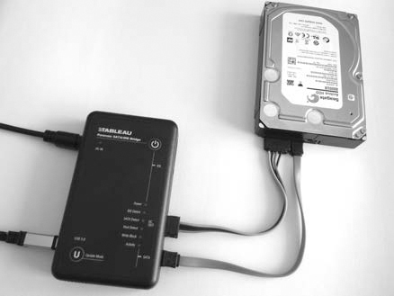
Figure 4-1: Portable SATA write blocker

Hardware write blockers usually have a switch or LED to indicate whether write blocking functionality is in operation. A photograph of a multifunctional write-blocking device designed to be built directly into the examiner workstation (Tableau by Guidance Software) is shown in Figure 4-2. It can protect SATA, SAS, IDE, FireWire, and USB drives.

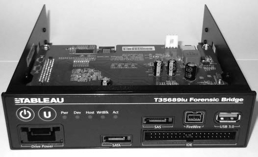
Figure 4-2: Multifunction drive bay write blocker

Write blockers can provide status information to the acquisition host system. An example is the tableau-parm tool (https://github.com/ecbftw/tableau-parm/), which can query the Tableau hardware write blocker for information. You can use this open source tool to verify the write-blocking status of a disk attached with a Tableau write blocker. For example:

$ sudo tableau-parm /dev/sdg
WARN: Requested 255 bytes but got 152 bytes)
## Bridge Information ##
chan_index: 0x00
chan_type: SATA
writes_permitted: FALSE
declare_write_blocked: TRUE
declare_write_errors: TRUE
bridge_serial: 000ECC550035F055
bridge_vendor: Tableau
bridge_model: T35u-R2
firmware_date: May 23 2014
firmware_time: 09:43:37

## Drive Information ##
drive_vendor: %00%00%00%00%00%00%00%00
drive_model: INTEL SSDSA2CW300G3
drive_serial: CVPR124600ET300EGN
drive_revision: 4PC10302

## Drive HPA/DCO/Security Information ##
security_in_use: FALSE
security_support: TRUE
hpa_in_use: FALSE
hpa_support: TRUE
dco_in_use: FALSE
dco_support: TRUE
drive_capacity: 586072368
hpa_capacity: 586072368
dco_capacity: 586072368

According to Tableau’s documentation, the drive_vendor field may not contain any information for some drives.⁵

During the final stages of editing this book, the first PCI Express write blockers appeared on the market. An example is shown here from Tableau. Attaching an NVME drive using a PCI Express write blocker produces the following dmesg output:

[194238.882053] usb 2-6: new SuperSpeed USB device number 5 using xhci_hcd
[194238.898642] usb 2-6: New USB device found, idVendor=13d7, idProduct=001e
[194238.898650] usb 2-6: New USB device strings: Mfr=1, Product=2, SerialNumber=3
[194238.898654] usb 2-6: Product: T356789u
[194238.898658] usb 2-6: Manufacturer: Tableau
[194238.898662] usb 2-6: SerialNumber: 0xecc3500671076
[194238.899830] usb-storage 2-6:1.0: USB Mass Storage device detected
[194238.901608] scsi host7: usb-storage 2-6:1.0
[194239.902816] scsi 7:0:0:0: Direct-Access     NVMe     INTEL SSDPEDMW40 0174
    PQ: 0 ANSI: 6
[194239.903611] sd 7:0:0:0: Attached scsi generic sg2 type 0
[194240.013810] sd 7:0:0:0: [sdc] 781422768 512-byte logical blocks: (400 GB/
    373 GiB)
[194240.123456] sd 7:0:0:0: [sdc] Write Protect is on
[194240.123466] sd 7:0:0:0: [sdc] Mode Sense: 17 00 80 00
[194240.233497] sd 7:0:0:0: [sdc] Write cache: disabled, read cache: enabled,
    doesn't support DPO or FUA
[194240.454298]  sdc: sdc1
[194240.673411] sd 7:0:0:0: [sdc] Attached SCSI disk

The write blocker operates as a USB3 bridge and makes the NVME drive available as a SCSI device. This particular write blocker supports PCI Express drives using both AHCI and NVME standards. The hardware interfaces supported are regular PCI Express slots (Figure 4-3) and M.2 (Figure 4-4). Standard adapters from mini-SAS to PCI Express or M.2 can be used to attach U.2 (SFF-8639) NVME drives. PCI write blockers with NVME support are also available from Wiebetech.

The primary advantage of hardware-based write blockers is their OS independence. They operate transparently and separately from the acquisition host, eliminating the need to maintain drivers or OS compatibility. This makes them ideal for use in a Linux acquisition environment.

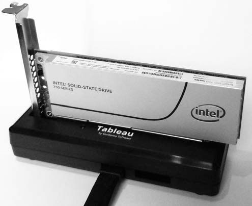
Figure 4-3: Write blocker dock for PCI Express slot drives

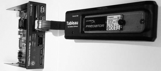
Figure 4-4: Multifunction write blocker and dock for PCI Express M.2 drives

Special thanks to Arina AG in Switzerland for providing the write blocker equipment used for test purposes in this book.

Software Write Blockers

Software write blockers have a somewhat controversial history. They’ve become increasingly difficult to develop and maintain with modern OSes. System updates by the OS vendor, configuration tweaks by the examiner, and additionally installed software all create a risk of disabling, overwriting, bypassing, or causing the failure of write-blocking functionality implemented in software.

Software write blockers are difficult to implement. Simply mounting a disk as read-only (mount -o ro) will not guarantee that the disk won’t be modified. The read-only property in this context refers to the filesystem, not the disk device. The kernel may still write to the disk for various reasons. Software write blocking must be implemented in the kernel, below the virtual filesystem layer and even below the other device drivers that implement a particular drive interface (AHCI for example). Several low-level software write-blocking methods have been used under Linux but with limited success.

Tools such as hdparm and blockdev can set a disk to read-only by setting a kernel flag. For example:

# hdparm -r1 /dev/sdk

/dev/sdk:
 setting readonly to 1 (on)
 readonly      =  1 (on)

The same flag can be set with blockdev, like this:

# blockdev --setro /dev/sdk

The method of setting kernel flags is dependent on properly configuring udev to make newly attached drives read-only before any other process has a chance to modify them.

A kernel patch has also been written to specifically implement forensic write-blocking functionality. You’ll find more information about it at https://github.com/msuhanov/Linux-write-blocker/. Several forensic boot CDs use Maxim Suhanov’s write-blocking kernel patch. The following helper script manages software write blocking on the DEFT Linux forensic boot CD:

% cat /usr/sbin/wrtblk
#!/bin/sh

# Mark a specified block device as read-only
[ $# -eq 1 ] || exit
[ ! -z "$1" ] || exit
bdev="$1"
[ -b "/dev/$bdev" ] || exit
[ ! -z $bdev##loop*$ ] || exit
blockdev --setro "/dev/$bdev" || logger "wrtblk: blockdev --setro /dev/$bdev
    failed!"

# Mark a parent block device as read-only
syspath=$(echo /sys/block/*/"$bdev")
[ "$syspath" = "/sys/block/*/$bdev" ] && exit
dir=$syspath%/*$
parent=$dir##*/$
[ -b "/dev/$parent" ] || exit
blockdev --setro "/dev/$parent" || logger "wrtblk: blockdev --setro /dev/$parent
    failed!"

The patch is implemented in the kernel and is turned on (and off) using helper scripts. The helper scripts simply use the blockdev command to mark the device as read-only.

NIST CFTT has performed software write blocker tool tests, which you’ll find at http://www.cftt.nist.gov/software_write_block.htm.

Hardware write blockers are still the safest and recommended method of protecting storage media during forensic acquisition.

Linux Forensic Boot CDs

The need to perform incident response and triage in the field has led to the development of bootable Linux CDs that contain the required software to perform such tasks. These CDs can boot a subject PC and access the locally attached storage using various forensic tools. Forensic boot CDs are designed to write protect discovered storage in the event it needs to be forensically imaged. You can make an attached disk writable by using a command (like wrtblk shown in the previous example), which is useful in acquiring an image when you attach an external destination disk. Forensic boot CDs also have network functionality and enable remote analysis and acquisition.

Forensic boot CDs are useful when:

• A PC is examined without opening it to remove a disk.

• A write blocker is not available.

• PCs need to be quickly checked during triage for a certain piece of evidence before deciding to image.

• Linux-based tools (Sleuth Kit, Foremost, and so on) are needed but not otherwise available.

• A forensic technician needs to remotely perform work via ssh.

Several popular forensic boot CDs that are currently maintained include:

• Kali Linux (formerly BackTrack), which is based on Debian: https://www.kali.org/

• Digital Evidence & Forensics Toolkit (DEFT), which is based on Ubuntu Linux: http://www.deftlinux.net/

• Pentoo, a forensic CD based on Gentoo Linux: http://pentoo.ch/

• C.A.I.N.E, Computer Forensics Linux Live Distro, which is based on Ubuntu Linux: http://www.caine-live.net/

Forensic boot CDs require a lot of work to maintain and test. Many other forensic boot CDs have been available in the past. Because of the changing landscape of forensic boot CDs, be sure to research and use the latest functional and maintained versions.

Media with Physical Read-Only Modes

Some storage media have a write-protect mechanism that can be useful in a forensic context. For example, most tapes have a sliding switch or tab that instructs the tape drive to treat them as read-only, as shown on the left of Figure 4-5. On the LTO-5 tape (bottom left), a closed tab indicates it is write protected; on the DAT160 tape (top left), an open tab indicates it is write protected.

SD memory cards have a lock switch that write protects the memory card, as shown on the right of Figure 4-5.

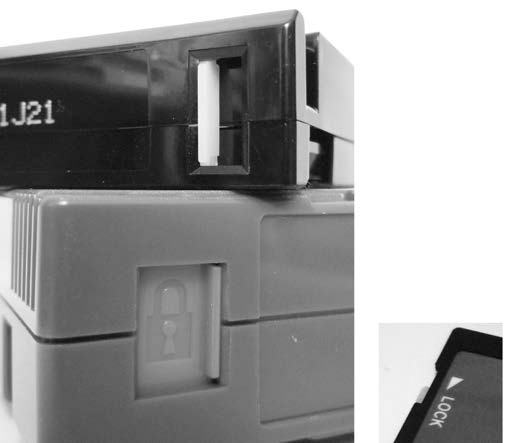
Figure 4-5: Write-protect tabs on tapes and SD cards

Older USB thumb drives may have a write-protect switch. Some very old IDE hard disks have a jumper that you can set to make the drive electronics treat the drive as read-only.

CD-ROMs, DVDs, and Blu-ray discs do not need a write blocker, because they are read-only by default. The simple act of accessing a rewritable disc will not make modifications to timestamps or other data on the disc; changes to these optical media must be explicitly burned to the disc.

Closing Thoughts

In this chapter, you learned how to set up basic auditing, activity logging, and task management. I covered topics such as naming conventions and scalable directory structures, as well as various challenges with image sizes, drive capacity planning, and performance and environmental issues. Finally, this chapter discussed the crucial component of forensic write blocking. You are now ready to attach a subject drive to the acquisition host in preparation for executing the forensic acquisition process.