Table of Contents for
Machine Learning with Python Cookbook
 Machine Learning with Python Cookbook
Published by
O'Reilly Media, Inc., 2018
Machine Learning with Python Cookbook
Published by
O'Reilly Media, Inc., 2018
- Cover
- nav
- Machine Learning with Python Cookbook
- Machine Learning with Python Cookbook
- Preface
- Vectors, Matrices, and Arrays
- Loading Data
- Data Wrangling
- Handling Numerical Data
- Handling Categorical Data
- Handling Text
- Handling Dates and Times
- Handling Images
- Dimensionality Reduction Using Feature Extraction
- Dimensionality Reduction Using Feature Selection
- Model Evaluation
- Model Selection
- Linear Regression
- Trees and Forests
- K-Nearest Neighbors
- Logistic Regression
- Support Vector Machines
- Naive Bayes
- Clustering
- Neural Networks
- Saving and Loading Trained Models
- Index
- About the Author
- Colophon
Chapter 20. Neural Networks
20.0 Introduction
At the heart of neural networks is the unit (also called a node or neuron). A unit takes in one or more inputs, multiplies each input by a parameter (also called a weight), sums the weighted input’s values along with some bias value (typically 1), and then feeds the value into an activation function. This output is then sent forward to the other neurals deeper in the neural network (if they exist).
Feedforward neural networks—also called multilayer perceptron—are the simplest artificial neural network used in any real-world setting. Neural networks can be visualized as a series of connected layers that form a network connecting an observation’s feature values at one end, and the target value (e.g., observation’s class) at the other end. The name feedforward comes from the fact that an observation’s feature values are fed “forward” through the network, with each layer successively transforming the feature values with the goal that the output at the end is the same as the target’s value.
Specifically, feedforward neural networks contain three types of layers of units. At the start of the neural network is an input layer where each unit contains an observation’s value for a single feature. For example, if an observation has 100 features, the input layer has 100 nodes. At the end of the neural network is the output layer, which transforms the output of the hidden layers into values useful for the task at hand. For example, if our goal was binary classification, we could use an output layer with a single unit that uses a sigmoid function to scale its own output to between 0 and 1, representing a predicted class probability. Between the input and output layers are the so-called “hidden” layers (which aren’t hidden at all). These hidden layers successively transform the feature values from the input layer to something that, once processed by the output layer, resembles the target class. Neural networks with many hidden layers (e.g., 10, 100, 1,000) are considered “deep” networks and their application is called deep learning.
Neural networks are typically created with all parameters initialized as small random values from a Gaussian or normal uniform. Once an observation (or more often a set number of observations called a batch) is fed through the network, the outputted value is compared with the observation’s true value using a loss function. This is called forward propagation. Next an algorithm goes “backward” through the network identifying how much each parameter contributed to the error between the predicted and true values, a process called backpropagation. At each parameter, the optimization algorithm determines how much each weight should be adjusted to improve the output.
Neural networks learn by repeating this process of forward propagation and backpropagation for every observation in the training data multiple times (each time all observations have been sent through the network is called an epoch and training typically consists of multiple epochs), iteratively updating the values of the parameters.
In this chapter, we will use the popular Python library Keras to build, train, and evaluate a variety of neural networks. Keras is a high-level library, using other libraries like TensorFlow and Theano as its “engine.” For us the advantage of Keras is that we can focus on network design and training, leaving the specifics of the tensor operations to the other libraries.
Neural networks created using Keras code can be trained using both CPUs (i.e., on your laptop) and GPUs (i.e., on a specialized deep learning computer). In the real world with real data, it is highly advisable to train neural networks using GPUs; however, for the sake of learning, all the neural networks in this book are small and simple enough to be trained on your laptop in only a few minutes. Just be aware that when we have larger networks and more training data, training using CPUs is significantly slower than training using GPUs.
20.1 Preprocessing Data for Neural Networks
Solution
Standardize each feature using scikit-learn’s StandardScaler:
# Load librariesfromsklearnimportpreprocessingimportnumpyasnp# Create featurefeatures=np.array([[-100.1,3240.1],[-200.2,-234.1],[5000.5,150.1],[6000.6,-125.1],[9000.9,-673.1]])# Create scalerscaler=preprocessing.StandardScaler()# Transform the featurefeatures_standardized=scaler.fit_transform(features)# Show featurefeatures_standardized
array([[-1.12541308,  1.96429418],
       [-1.15329466, -0.50068741],
       [ 0.29529406, -0.22809346],
       [ 0.57385917, -0.42335076],
       [ 1.40955451, -0.81216255]])
Discussion
While this recipe is very similar to Recipe 4.3, it is worth repeating because of how important it is for neural networks. Typically, a neural network’s parameters are initialized (i.e., created) as small random numbers. Neural networks often behave poorly when the feature values are much larger than parameter values. Furthermore, since an observation’s feature values are combined as they pass through individual units, it is important that all features have the same scale.
For these reasons, it is best practice (although not always necessary;
for example, when we have all binary features) to standardize each
feature such that the feature’s values have the mean of 0 and the
standard deviation of 1. This can be easily accomplished with
scikit-learn’s StandardScaler.
You can see the effect of the standardization by checking the mean and standard deviation of our first features:
# Print mean and standard deviation("Mean:",round(features_standardized[:,0].mean()))('"Standard deviation:", features_standardized[:,0].std())
Mean: 0.0
Standard deviation: 1.0
20.2 Designing a Neural Network
Solution
Use Keras’ Sequential model:
# Load librariesfromkerasimportmodelsfromkerasimportlayers# Start neural networknetwork=models.Sequential()# Add fully connected layer with a ReLU activation functionnetwork.add(layers.Dense(units=16,activation="relu",input_shape=(10,)))# Add fully connected layer with a ReLU activation functionnetwork.add(layers.Dense(units=16,activation="relu"))# Add fully connected layer with a sigmoid activation functionnetwork.add(layers.Dense(units=1,activation="sigmoid"))# Compile neural networknetwork.compile(loss="binary_crossentropy",# Cross-entropyoptimizer="rmsprop",# Root Mean Square Propagationmetrics=["accuracy"])# Accuracy performance metric
Using TensorFlow backend.
Discussion
Neural networks consist of layers of units. However, there is incredible variety in the types of layers and how they are combined to form the network’s architecture. At present, while there are commonly used architecture patterns (which we will cover in this chapter), the truth is that selecting the right architecture is mostly an art and the topic of much research.
To construct a feedforward neural network in Keras, we need to make a number of choices about both the network architecture and training process. Remember that each unit in the hidden layers:
-
Receives a number of inputs.
-
Weights each input by a parameter value.
-
Sums together all weighted inputs along with some bias (typically 1).
-
Most often then applies some function (called an activation function).
-
Sends the output on to units in the next layer.
First, for each layer in the hidden and output layers we must define the number of units to include in the layer and the activation function. Overall, the more units we have in a layer, the more our network is able to learn complex patterns. However, more units might make our network overfit the training data in a way detrimental to the performance on the test data.
For hidden layers, a popular activation function is the rectified linear unit (ReLU):
where z is the sum of the weighted inputs and bias. As we can see, if z is greater than 0, the activation function returns z; otherwise, the function returns 0. This simple activation function has a number of desirable properties (a discussion of which is beyond the scope of this book) and this has made it a popular choice in neural networks. We should be aware, however, that many dozens of activation functions exist.
Second, we need to define the number of hidden layers to use in the network. More layers allow the network to learn more complex relationships, but with a computational cost.
Third, we have to define the structure of the activation function (if any) of the output layer. The nature of the output function is often determined by the goal of the network. Here are some common output layer patterns:
- Binary classification
- Multiclass classification
-
k units (where k is the number of target classes) and a softmax activation function.
- Regression
Fourth, we need to define a loss function (the function that measures how well a predicted value matches the true value); this is again often determined by the problem type:
- Binary classification
-
Binary cross-entropy.
- Multiclass classification
-
Categorical cross-entropy.
- Regression
-
Mean square error.
Fifth, we have to define an optimizer, which intuitively can be thought of as our strategy “walking around” the loss function to find the parameter values that produce the lowest error. Common choices for optimizers are stochastic gradient descent, stochastic gradient descent with momentum, root mean square propagation, and adaptive moment estimation (more information on these optimizers in “See Also”).
Sixth, we can select one or more metrics to use to evaluate the performance, such as accuracy.
Keras offers two ways for creating neural networks. Keras’ sequential model creates neural networks by stacking together layers. An alternative method for creating neural networks is called the functional API, but that is more for researchers rather than practitioners.
In our solution, we created a two-layer neural network (when counting
layers we don’t include the input layer because it does not have any
parameters to learn) using Keras’ sequential model. Each layer is
“dense” (also called fully connected), meaning that all the units in the previous layer are connected to all the neurals in the next layer. In the first hidden layer we set units=16, meaning that layer contains 16 units with ReLU activation functions: activation='relu'. In Keras, the first hidden layer of any network has to include an input_shape parameter, which is the shape of feature data. For example, (10,) tells the first layer to expect each observation to have 10 feature values. Our second layer is the same as the first, without the need for the input_shape parameter. This network is designed for binary classification so the output layer contains only one unit with a sigmoid activation function, which constrains the output to between 0 and 1 (representing the probability an observation is class 1).
Finally, before we can train our model, we need to tell Keras how we
want our network to learn. We do this using the compile method, with our optimization algorithm (RMSProp), loss function (binary_crossentropy), and one or more performance metrics.
20.3 Training a Binary Classifier
Solution
Use Keras to construct a feedforward neural network and train it using
the fit method:
# Load librariesimportnumpyasnpfromkeras.datasetsimportimdbfromkeras.preprocessing.textimportTokenizerfromkerasimportmodelsfromkerasimportlayers# Set random seednp.random.seed(0)# Set the number of features we wantnumber_of_features=1000# Load data and target vector from movie review data(data_train,target_train),(data_test,target_test)=imdb.load_data(num_words=number_of_features)# Convert movie review data to one-hot encoded feature matrixtokenizer=Tokenizer(num_words=number_of_features)features_train=tokenizer.sequences_to_matrix(data_train,mode="binary")features_test=tokenizer.sequences_to_matrix(data_test,mode="binary")# Start neural networknetwork=models.Sequential()# Add fully connected layer with a ReLU activation functionnetwork.add(layers.Dense(units=16,activation="relu",input_shape=(number_of_features,)))# Add fully connected layer with a ReLU activation functionnetwork.add(layers.Dense(units=16,activation="relu"))# Add fully connected layer with a sigmoid activation functionnetwork.add(layers.Dense(units=1,activation="sigmoid"))# Compile neural networknetwork.compile(loss="binary_crossentropy",# Cross-entropyoptimizer="rmsprop",# Root Mean Square Propagationmetrics=["accuracy"])# Accuracy performance metric# Train neural networkhistory=network.fit(features_train,# Featurestarget_train,# Target vectorepochs=3,# Number of epochsverbose=1,# Print description after each epochbatch_size=100,# Number of observations per batchvalidation_data=(features_test,target_test))# Test data
Using TensorFlow backend.


Train on 25000 samples, validate on 25000 samples
Epoch 1/3
25000/25000 [==============================]
- 1s - loss: 0.4215 - acc: 0.8105 - val_loss: 0.3386 - val_acc: 0.8555
Epoch 2/3
25000/25000 [==============================]
- 1s - loss: 0.3242 - acc: 0.8645 - val_loss: 0.3258 - val_acc: 0.8633
Epoch 3/3
25000/25000 [==============================]
- 1s - loss: 0.3121 - acc: 0.8699 - val_loss: 0.3265 - val_acc: 0.8599
Discussion
In Recipe 20.2, we discussed how to construct a neural network using Keras’ sequential model. In this recipe we train that neural network using real data. Specifically, we use 50,000 movie reviews (25,000 as training data, 25,000 held out for testing), categorized as positive or negative. We convert the text of the reviews into 5,000 binary features indicating the presence of one of the 1,000 most frequent words. Put more simply, our neural networks will use 25,000 observations, each with 1,000 features, to predict if a movie review is positive or negative.
The neural network we are using is the same as the one in Recipe 20.2 (see there for a detailed explanation). The only addition is that in that recipe we only created the neural network, we didn’t train it.
In Keras, we train our neural network using the fit method. There are
six significant parameters to define. The first two parameters are the
features and target vector of the training data. We can view the shape
of feature matrix using shape:
# View shape of feature matrixfeatures_train.shape
(25000, 1000)
The epochs parameter defines how many epochs to use when training the
data. verbose determines how much information is outputted during the
training process, with 0 being no output, 1 outputting a progress bar,
and 2 one log line per epoch. batch_size sets the number of
observations to propagate through the network before updating the
parameters.
Finally, we held out a test set of data to use to evaluate the model.
These test features and test target vector can be arguments of
validation_data, which will use them for evaluation. Alternatively, we
could have used validation_split to define what fraction of the
training data we want to hold out for evaluation.
In scikit-learn the fit method returned a trained model, but in Keras
the fit method returns a History object containing the loss values
and performance metrics at each epoch.
20.4 Training a Multiclass Classifier
Solution
Use Keras to construct a feedforward neural network with an output layer with softmax activation functions:
# Load librariesimportnumpyasnpfromkeras.datasetsimportreutersfromkeras.utils.np_utilsimportto_categoricalfromkeras.preprocessing.textimportTokenizerfromkerasimportmodelsfromkerasimportlayers# Set random seednp.random.seed(0)# Set the number of features we wantnumber_of_features=5000# Load feature and target datadata=reuters.load_data(num_words=number_of_features)(data_train,target_vector_train),(data_test,target_vector_test)=data# Convert feature data to a one-hot encoded feature matrixtokenizer=Tokenizer(num_words=number_of_features)features_train=tokenizer.sequences_to_matrix(data_train,mode="binary")features_test=tokenizer.sequences_to_matrix(data_test,mode="binary")# One-hot encode target vector to create a target matrixtarget_train=to_categorical(target_vector_train)target_test=to_categorical(target_vector_test)# Start neural networknetwork=models.Sequential()# Add fully connected layer with a ReLU activation functionnetwork.add(layers.Dense(units=100,activation="relu",input_shape=(number_of_features,)))# Add fully connected layer with a ReLU activation functionnetwork.add(layers.Dense(units=100,activation="relu"))# Add fully connected layer with a softmax activation functionnetwork.add(layers.Dense(units=46,activation="softmax"))# Compile neural networknetwork.compile(loss="categorical_crossentropy",# Cross-entropyoptimizer="rmsprop",# Root Mean Square Propagationmetrics=["accuracy"])# Accuracy performance metric# Train neural networkhistory=network.fit(features_train,# Featurestarget_train,# Targetepochs=3,# Three epochsverbose=0,# No outputbatch_size=100,# Number of observations per batchvalidation_data=(features_test,target_test))# Test data
Using TensorFlow backend.
Discussion
In this solution we created a similar neural network to the binary classifier from the last recipe, but with some notable changes. First, our data is 11,228 Reuters newswires. Each newswire is categorized into 46 topics. We prepared our feature data by converting the newswires into 5,000 binary features (denoting the presence of a certain word in the newswires). We prepared the target data by one-hot encoding it so that we obtain a target matrix denoting which of the 46 classes an observation belongs to:
# View target matrixtarget_train
array([[ 0.,  0.,  0., ...,  0.,  0.,  0.],
       [ 0.,  0.,  0., ...,  0.,  0.,  0.],
       [ 0.,  0.,  0., ...,  0.,  0.,  0.],
       ...,
       [ 0.,  0.,  0., ...,  0.,  0.,  0.],
       [ 0.,  0.,  0., ...,  0.,  0.,  0.],
       [ 0.,  0.,  0., ...,  0.,  0.,  0.]])
Second, we increased the number of units in each of the hidden layers to help the neural network represent the more complex relationship between the 46 classes.
Third, since this is a multiclass classification problem, we used an output layer with 46 units (one per class) containing a softmax activation function. The softmax activation function will return an array of 46 values summing to 1. These 46 values represent an observation’s probability of being a member of each of the 46 classes.
Fourth, we used a loss function suited to multiclass classification, the
categorical cross-entropy loss function, categorical_crossentropy.
20.5 Training a Regressor
Solution
Use Keras to construct a feedforward neural network with a single output unit and no activation function:
# Load librariesimportnumpyasnpfromkeras.preprocessing.textimportTokenizerfromkerasimportmodelsfromkerasimportlayersfromsklearn.datasetsimportmake_regressionfromsklearn.model_selectionimporttrain_test_splitfromsklearnimportpreprocessing# Set random seednp.random.seed(0)# Generate features matrix and target vectorfeatures,target=make_regression(n_samples=10000,n_features=3,n_informative=3,n_targets=1,noise=0.0,random_state=0)# Divide our data into training and test setsfeatures_train,features_test,target_train,target_test=train_test_split(features,target,test_size=0.33,random_state=0)# Start neural networknetwork=models.Sequential()# Add fully connected layer with a ReLU activation functionnetwork.add(layers.Dense(units=32,activation="relu",input_shape=(features_train.shape[1],)))# Add fully connected layer with a ReLU activation functionnetwork.add(layers.Dense(units=32,activation="relu"))# Add fully connected layer with no activation functionnetwork.add(layers.Dense(units=1))# Compile neural networknetwork.compile(loss="mse",# Mean squared erroroptimizer="RMSprop",# Optimization algorithmmetrics=["mse"])# Mean squared error# Train neural networkhistory=network.fit(features_train,# Featurestarget_train,# Target vectorepochs=10,# Number of epochsverbose=0,# No outputbatch_size=100,# Number of observations per batchvalidation_data=(features_test,target_test))# Test data
Using TensorFlow backend.
Discussion
It is completely possible to create a neural network to predict continuous values instead of class probabilities. In the case of our binary classifier (Recipe 20.3) we used an output layer with a single unit and a sigmoid activation function to produce a probability that an observation was class 1. Importantly, the sigmoid activation function constrained the outputted value to between 0 and 1. If we remove that constraint by having no activation function, we allow the output to be a continuous value.
Furthermore, because we are training a regression, we should use an appropriate loss function and evaluation metric, in our case the mean square error:
where n is the number of observations; yi is the true value of the target we are trying to predict, y, for observation i; and ŷi is the model’s predicted value for yi.
Finally, because we are using simulated data using scikit-learn,
make_regression, we didn’t have to standardize the features. It should be noted, however, that in almost all real-world cases standardization would be necessary.
20.6 Making Predictions
Solution
Use Keras to construct a feedforward neural network, then make
predictions using predict:
# Load librariesimportnumpyasnpfromkeras.datasetsimportimdbfromkeras.preprocessing.textimportTokenizerfromkerasimportmodelsfromkerasimportlayers# Set random seednp.random.seed(0)# Set the number of features we wantnumber_of_features=10000# Load data and target vector from IMDB movie data(data_train,target_train),(data_test,target_test)=imdb.load_data(num_words=number_of_features)# Convert IMDB data to a one-hot encoded feature matrixtokenizer=Tokenizer(num_words=number_of_features)features_train=tokenizer.sequences_to_matrix(data_train,mode="binary")features_test=tokenizer.sequences_to_matrix(data_test,mode="binary")# Start neural networknetwork=models.Sequential()# Add fully connected layer with a ReLU activation functionnetwork.add(layers.Dense(units=16,activation="relu",input_shape=(number_of_features,)))# Add fully connected layer with a ReLU activation functionnetwork.add(layers.Dense(units=16,activation="relu"))# Add fully connected layer with a sigmoid activation functionnetwork.add(layers.Dense(units=1,activation="sigmoid"))# Compile neural networknetwork.compile(loss="binary_crossentropy",# Cross-entropyoptimizer="rmsprop",# Root Mean Square Propagationmetrics=["accuracy"])# Accuracy performance metric# Train neural networkhistory=network.fit(features_train,# Featurestarget_train,# Target vectorepochs=3,# Number of epochsverbose=0,# No outputbatch_size=100,# Number of observations per batchvalidation_data=(features_test,target_test))# Test data# Predict classes of test setpredicted_target=network.predict(features_test)
Using TensorFlow backend.
Discussion
Making predictions is easy in Keras. Once we have trained our neural
network we can use the predict method, which takes as an argument a set
of features and returns the predicted output for each observation. In
our solution our neural network is set up for binary classification so
the predicted output is the probability of being class 1. Observations
with predicted values very close to 1 are highly likely to be class 1,
while observations with predicted values very close to 0 are highly
likely to be class 0. For example, this is the predicted probability that the
first observation in our test feature matrix is class 1:
# View the probability the first observation is class 1predicted_target[0]
array([ 0.83937484], dtype=float32)
20.7 Visualize Training History
Solution
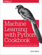
Use Matplotlib to visualize the loss of the test and training set over each epoch:
# Load librariesimportnumpyasnpfromkeras.datasetsimportimdbfromkeras.preprocessing.textimportTokenizerfromkerasimportmodelsfromkerasimportlayersimportmatplotlib.pyplotasplt# Set random seednp.random.seed(0)# Set the number of features we wantnumber_of_features=10000# Load data and target vector from movie review data(data_train,target_train),(data_test,target_test)=imdb.load_data(num_words=number_of_features)# Convert movie review data to a one-hot encoded feature matrixtokenizer=Tokenizer(num_words=number_of_features)features_train=tokenizer.sequences_to_matrix(data_train,mode="binary")features_test=tokenizer.sequences_to_matrix(data_test,mode="binary")# Start neural networknetwork=models.Sequential()# Add fully connected layer with a ReLU activation functionnetwork.add(layers.Dense(units=16,activation="relu",input_shape=(number_of_features,)))# Add fully connected layer with a ReLU activation functionnetwork.add(layers.Dense(units=16,activation="relu"))# Add fully connected layer with a sigmoid activation functionnetwork.add(layers.Dense(units=1,activation="sigmoid"))# Compile neural networknetwork.compile(loss="binary_crossentropy",# Cross-entropyoptimizer="rmsprop",# Root Mean Square Propagationmetrics=["accuracy"])# Accuracy performance metric# Train neural networkhistory=network.fit(features_train,# Featurestarget_train,# Targetepochs=15,# Number of epochsverbose=0,# No outputbatch_size=1000,# Number of observations per batchvalidation_data=(features_test,target_test))# Test data# Get training and test loss historiestraining_loss=history.history["loss"]test_loss=history.history["val_loss"]# Create count of the number of epochsepoch_count=range(1,len(training_loss)+1)# Visualize loss historyplt.plot(epoch_count,training_loss,"r--")plt.plot(epoch_count,test_loss,"b-")plt.legend(["Training Loss","Test Loss"])plt.xlabel("Epoch")plt.ylabel("Loss")plt.show();
Using TensorFlow backend.
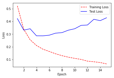
Alternatively, we can use the same approach to visualize the training and test accuracy over each epoch:
# Get training and test accuracy historiestraining_accuracy=history.history["acc"]test_accuracy=history.history["val_acc"]plt.plot(epoch_count,training_accuracy,"r--")plt.plot(epoch_count,test_accuracy,"b-")# Visualize accuracy historyplt.legend(["Training Accuracy","Test Accuracy"])plt.xlabel("Epoch")plt.ylabel("Accuracy Score")plt.show();
Discussion
When our neural network is new, it will have a poor performance. As the neural network learns on the training data, the model’s error on both the training and test set will tend to increase. However, at a certain point the neural network starts “memorizing” the training data, and overfits. When this starts happening, the training error will decrease while the test error will start increasing. Therefore, in many cases there is a “sweet spot” where the test error (which is the error we mainly care about) is at its lowest point. This effect can be plainly seen in the solution where we visualize the training and test loss at each epoch. Note that the test error is lowest around epoch five, after which the training loss continues to increase while the test loss starts increasing. At this point onward, the model is overfitting.
20.8 Reducing Overfitting with Weight Regularization
Solution
Try penalizing the parameters of the network, also called weight regularization:
# Load librariesimportnumpyasnpfromkeras.datasetsimportimdbfromkeras.preprocessing.textimportTokenizerfromkerasimportmodelsfromkerasimportlayersfromkerasimportregularizers# Set random seednp.random.seed(0)# Set the number of features we wantnumber_of_features=1000# Load data and target vector from movie review data(data_train,target_train),(data_test,target_test)=imdb.load_data(num_words=number_of_features)# Convert movie review data to a one-hot encoded feature matrixtokenizer=Tokenizer(num_words=number_of_features)features_train=tokenizer.sequences_to_matrix(data_train,mode="binary")features_test=tokenizer.sequences_to_matrix(data_test,mode="binary")# Start neural networknetwork=models.Sequential()# Add fully connected layer with a ReLU activation functionnetwork.add(layers.Dense(units=16,activation="relu",kernel_regularizer=regularizers.l2(0.01),input_shape=(number_of_features,)))# Add fully connected layer with a ReLU activation functionnetwork.add(layers.Dense(units=16,kernel_regularizer=regularizers.l2(0.01),activation="relu"))# Add fully connected layer with a sigmoid activation functionnetwork.add(layers.Dense(units=1,activation="sigmoid"))# Compile neural networknetwork.compile(loss="binary_crossentropy",# Cross-entropyoptimizer="rmsprop",# Root Mean Square Propagationmetrics=["accuracy"])# Accuracy performance metric# Train neural networkhistory=network.fit(features_train,# Featurestarget_train,# Target vectorepochs=3,# Number of epochsverbose=0,# No outputbatch_size=100,# Number of observations per batchvalidation_data=(features_test,target_test))# Test data
Using TensorFlow backend.
Discussion
One strategy to combat overfitting neural networks is by penalizing the parameters (i.e., weights) of the neural network such that they are driven to be small values—creating a simpler model less prone to overfit. This method is called weight regularization or weight decay. More specifically, in weight regularization a penalty is added to the loss function, such as the L2 norm.
In Keras, we can add a weight regularization by including using
kernel_regularizer=regularizers.l2(0.01) in a layer’s
parameters. In this example, 0.01 determines how much we penalize
higher parameter values.
20.9 Reducing Overfitting with Early Stopping
Problem
You want to reduce overfitting.
Solution
Try stopping training when the test loss stops decreasing, a strategy called early stopping:
# Load librariesimportnumpyasnpfromkeras.datasetsimportimdbfromkeras.preprocessing.textimportTokenizerfromkerasimportmodelsfromkerasimportlayersfromkeras.callbacksimportEarlyStopping,ModelCheckpoint# Set random seednp.random.seed(0)# Set the number of features we wantnumber_of_features=1000# Load data and target vector from movie review data(data_train,target_train),(data_test,target_test)=imdb.load_data(num_words=number_of_features)# Convert movie review data to a one-hot encoded feature matrixtokenizer=Tokenizer(num_words=number_of_features)features_train=tokenizer.sequences_to_matrix(data_train,mode="binary")features_test=tokenizer.sequences_to_matrix(data_test,mode="binary")# Start neural networknetwork=models.Sequential()# Add fully connected layer with a ReLU activation functionnetwork.add(layers.Dense(units=16,activation="relu",input_shape=(number_of_features,)))# Add fully connected layer with a ReLU activation functionnetwork.add(layers.Dense(units=16,activation="relu"))# Add fully connected layer with a sigmoid activation functionnetwork.add(layers.Dense(units=1,activation="sigmoid"))# Compile neural networknetwork.compile(loss="binary_crossentropy",# Cross-entropyoptimizer="rmsprop",# Root Mean Square Propagationmetrics=["accuracy"])# Accuracy performance metric# Set callback functions to early stop training and save the best model so farcallbacks=[EarlyStopping(monitor="val_loss",patience=2),ModelCheckpoint(filepath="best_model.h5",monitor="val_loss",save_best_only=True)]# Train neural networkhistory=network.fit(features_train,# Featurestarget_train,# Target vectorepochs=20,# Number of epochscallbacks=callbacks,# Early stoppingverbose=0,# Print description after each epochbatch_size=100,# Number of observations per batchvalidation_data=(features_test,target_test))# Test data
Using TensorFlow backend.
Discussion
As we discussed in Recipe 20.7, typically in the first training epochs both the training and test errors will decrease, but at some point the network will start “memorizing” the training data, causing the training error to continue to decrease even while the test error starts increasing. Because of this phenomenon, one of the most common and very effective methods to counter overfitting is to monitor the training process and stop training when the test error starts to increase. This strategy is called early stopping.
In Keras, we can implement early stopping as a callback function.
Callbacks are functions that can be applied at certain stages of the training process, such as at the end of each epoch. Specifically, in our solution, we included EarlyStopping(monitor='val_loss', patience=2) to define that we wanted to monitor the test (validation) loss at each epoch and after the test loss has not improved after two epochs, training is interrupted. However, since we set patience=2, we won’t get the best model, but the model two epochs after the best model. Therefore, optionally, we can include a second operation, ModelCheckpoint, which saves the model to a file after every checkpoint
(which can be useful in case a multiday training session is interrupted
for some reason). It would be helpful for us, if we set save_best_only=True, because then ModelCheckpoint will only save the best model.
20.10 Reducing Overfitting with Dropout
Solution
Introduce noise into your network’s architecture using dropout:
# Load librariesimportnumpyasnpfromkeras.datasetsimportimdbfromkeras.preprocessing.textimportTokenizerfromkerasimportmodelsfromkerasimportlayers# Set random seednp.random.seed(0)# Set the number of features we wantnumber_of_features=1000# Load data and target vector from movie review data(data_train,target_train),(data_test,target_test)=imdb.load_data(num_words=number_of_features)# Convert movie review data to a one-hot encoded feature matrixtokenizer=Tokenizer(num_words=number_of_features)features_train=tokenizer.sequences_to_matrix(data_train,mode="binary")features_test=tokenizer.sequences_to_matrix(data_test,mode="binary")# Start neural networknetwork=models.Sequential()# Add a dropout layer for input layernetwork.add(layers.Dropout(0.2,input_shape=(number_of_features,)))# Add fully connected layer with a ReLU activation functionnetwork.add(layers.Dense(units=16,activation="relu"))# Add a dropout layer for previous hidden layernetwork.add(layers.Dropout(0.5))# Add fully connected layer with a ReLU activation functionnetwork.add(layers.Dense(units=16,activation="relu"))# Add a dropout layer for previous hidden layernetwork.add(layers.Dropout(0.5))# Add fully connected layer with a sigmoid activation functionnetwork.add(layers.Dense(units=1,activation="sigmoid"))# Compile neural networknetwork.compile(loss="binary_crossentropy",# Cross-entropyoptimizer="rmsprop",# Root Mean Square Propagationmetrics=["accuracy"])# Accuracy performance metric# Train neural networkhistory=network.fit(features_train,# Featurestarget_train,# Target vectorepochs=3,# Number of epochsverbose=0,# No outputbatch_size=100,# Number of observations per batchvalidation_data=(features_test,target_test))# Test data
Using TensorFlow backend.
Discussion
Dropout is a popular and powerful method for regularizing neural networks. In dropout, every time a batch of observations is created for training, a proportion of the units in one or more layers is multiplied by zero (i.e., dropped). In this setting, every batch is trained on the same network (e.g., the same parameters), but each batch is confronted by a slightly different version of that network’s architecture.
Dropout is effective because by constantly and randomly dropping units in each batch, it forces units to learn parameter values able to perform under a wide variety of network architectures. That is, they learn to be robust to disruptions (i.e., noise) in the other hidden units, and this prevents the network from simply memorizing the training data.
It is possible to add dropout to both the hidden and input layers. When an input layer is dropped, its feature value is not introduced into the network for that batch. A common choice for the portion of units to drop is 0.2 for input units and 0.5 for hidden units.
In Keras, we can implement dropout by adding Dropout layers into our
network architecture. Each Dropout layer will drop a user-defined
hyperparameter of units in the previous layer every batch. Remember in
Keras the input layer is assumed to be the first layer and not added
using add. Therefore, if we want to add dropout to the input
layer, the first layer we add in our network architecture is a dropout layer. This layer contains both the proportion of the input layer’s units to drop 0.2 and input_shape defining the shape of the observation data. Next, we add a dropout layer with 0.5 after each of the hidden layers.
20.11 Saving Model Training Progress
Solution
Use the callback function ModelCheckpoint to save the model after
every epoch:
# Load librariesimportnumpyasnpfromkeras.datasetsimportimdbfromkeras.preprocessing.textimportTokenizerfromkerasimportmodelsfromkerasimportlayersfromkeras.callbacksimportModelCheckpoint# Set random seednp.random.seed(0)# Set the number of features we wantnumber_of_features=1000# Load data and target vector from movie review data(data_train,target_train),(data_test,target_test)=imdb.load_data(num_words=number_of_features)# Convert movie review data to a one-hot encoded feature matrixtokenizer=Tokenizer(num_words=number_of_features)features_train=tokenizer.sequences_to_matrix(data_train,mode="binary")features_test=tokenizer.sequences_to_matrix(data_test,mode="binary")# Start neural networknetwork=models.Sequential()# Add fully connected layer with a ReLU activation functionnetwork.add(layers.Dense(units=16,activation="relu",input_shape=(number_of_features,)))# Add fully connected layer with a ReLU activation functionnetwork.add(layers.Dense(units=16,activation="relu"))# Add fully connected layer with a sigmoid activation functionnetwork.add(layers.Dense(units=1,activation="sigmoid"))# Compile neural networknetwork.compile(loss="binary_crossentropy",# Cross-entropyoptimizer="rmsprop",# Root Mean Square Propagationmetrics=["accuracy"])# Accuracy performance metric# Set callback functions to early stop training and save the best model so farcheckpoint=[ModelCheckpoint(filepath="models.hdf5")]# Train neural networkhistory=network.fit(features_train,# Featurestarget_train,# Target vectorepochs=3,# Number of epochscallbacks=checkpoint,# Checkpointverbose=0,# No outputbatch_size=100,# Number of observations per batchvalidation_data=(features_test,target_test))# Test data
Using TensorFlow backend.
Discussion
In Recipe 20.8 we used the callback function ModelCheckpoint in
conjunction with EarlyStopping to end monitoring and end training when
the test error stopped improving. However, there is another, more
mundane reason for using ModelCheckpoint. In the real world, it is
common for neural networks to train for hours or even days. During that
time a lot can go wrong: computers can lose power, servers can crash, or
inconsiderate graduate students can close your laptop.
ModelCheckpoint alleviates this problem by saving the model after
every epoch. Specifically, after every epoch ModelCheckpoint saves a
model to the location specified by the filepath parameter. If we
include only a filename (e.g., models.hdf5) that file will be
overridden with the latest model every epoch. If we only wanted to save
the best model according to the performance of some loss function, we
can set save_best_only=True and monitor='val_loss' to not override a
file if the model has a worse test loss than the previous model.
Alternatively, we can save every epoch’s model as its own file by
including the epoch number and test loss score into the filename itself.
For example, if we set filepath to
model_{epoch:02d}_{val_loss:.2f}.hdf5, the name of the file containing
the model saved after the 11th epoch with a test loss value of 0.33
would be model_10_0.35.hdf5 (notice that the epoch number is
0-indexed).
20.12 k-Fold Cross-Validating Neural Networks
Solution
Often k-fold cross-validating neural networks is neither necessary nor advisable. However, if it is appropriate: use Keras’ scikit-learn wrapper to allow Keras’ sequential models to use the scikit-learn API:
# Load librariesimportnumpyasnpfromkerasimportmodelsfromkerasimportlayersfromkeras.wrappers.scikit_learnimportKerasClassifierfromsklearn.model_selectionimportcross_val_scorefromsklearn.datasetsimportmake_classification# Set random seednp.random.seed(0)# Number of featuresnumber_of_features=100# Generate features matrix and target vectorfeatures,target=make_classification(n_samples=10000,n_features=number_of_features,n_informative=3,n_redundant=0,n_classes=2,weights=[.5,.5],random_state=0)# Create function returning a compiled networkdefcreate_network():# Start neural networknetwork=models.Sequential()# Add fully connected layer with a ReLU activation functionnetwork.add(layers.Dense(units=16,activation="relu",input_shape=(number_of_features,)))# Add fully connected layer with a ReLU activation functionnetwork.add(layers.Dense(units=16,activation="relu"))# Add fully connected layer with a sigmoid activation functionnetwork.add(layers.Dense(units=1,activation="sigmoid"))# Compile neural networknetwork.compile(loss="binary_crossentropy",# Cross-entropyoptimizer="rmsprop",# Root Mean Square Propagationmetrics=["accuracy"])# Accuracy performance metric# Return compiled networkreturnnetwork# Wrap Keras model so it can be used by scikit-learnneural_network=KerasClassifier(build_fn=create_network,epochs=10,batch_size=100,verbose=0)# Evaluate neural network using three-fold cross-validationcross_val_score(neural_network,features,target,cv=3)
Using TensorFlow backend.

array([ 0.90461907,  0.77437743,  0.87068707])
Discussion
Theoretically, there is no reason we cannot use cross-validation to evaluate neural networks. However, neural networks are often used on very large data and can take hours or even days to train. For this reason, if the training time is long, adding the computational expense of k-fold cross-validation is unadvisable. For example, a model normally taking one day to train would take 10 days to evaluate using 10-fold cross-validation. If we have large data, it is often appropriate to simply evaluate the neural network on some test set.
If we have smaller data, k-fold cross-validation can be useful to maximize our ability to evaluate the neural network’s performance. This is possible in Keras because we can “wrap” any neural network such that it can use the evaluation features available in scikit-learn, including k-fold cross-validation. To accomplish this, we first have to create a function that returns a compiled neural network. Next we use KerasClassifier (if we have a classifier; if we have a regressor we can use KerasRegressor) to wrap the model so it can be used by scikit-learn. After this, we can use our neural network like any other scikit-learn learning algorithm (e.g., random forests, logistic regression). In our solution, we used cross_val_score to run a three-fold cross-validation on our neural network.
20.13 Tuning Neural Networks
Solution
Combine a Keras neural network with scikit-learn’s model selection tools like GridSearchCV:
# Load librariesimportnumpyasnpfromkerasimportmodelsfromkerasimportlayersfromkeras.wrappers.scikit_learnimportKerasClassifierfromsklearn.model_selectionimportGridSearchCVfromsklearn.datasetsimportmake_classification# Set random seednp.random.seed(0)# Number of featuresnumber_of_features=100# Generate features matrix and target vectorfeatures,target=make_classification(n_samples=10000,n_features=number_of_features,n_informative=3,n_redundant=0,n_classes=2,weights=[.5,.5],random_state=0)# Create function returning a compiled networkdefcreate_network(optimizer="rmsprop"):# Start neural networknetwork=models.Sequential()# Add fully connected layer with a ReLU activation functionnetwork.add(layers.Dense(units=16,activation="relu",input_shape=(number_of_features,)))# Add fully connected layer with a ReLU activation functionnetwork.add(layers.Dense(units=16,activation="relu"))# Add fully connected layer with a sigmoid activation functionnetwork.add(layers.Dense(units=1,activation="sigmoid"))# Compile neural networknetwork.compile(loss="binary_crossentropy",# Cross-entropyoptimizer=optimizer,# Optimizermetrics=["accuracy"])# Accuracy performance metric# Return compiled networkreturnnetwork# Wrap Keras model so it can be used by scikit-learnneural_network=KerasClassifier(build_fn=create_network,verbose=0)# Create hyperparameter spaceepochs=[5,10]batches=[5,10,100]optimizers=["rmsprop","adam"]# Create hyperparameter optionshyperparameters=dict(optimizer=optimizers,epochs=epochs,batch_size=batches)# Create grid searchgrid=GridSearchCV(estimator=neural_network,param_grid=hyperparameters)# Fit grid searchgrid_result=grid.fit(features,target)
Using TensorFlow backend.
Discussion
In Recipes 12.1 and 12.2, we covered using scikit-learn’s model selection techniques to identify the best hyperparameters of a scikit-learn model. In Recipe 20.12 we learned that we can wrap our neural network so it can use the scikit-learn API. In this recipe we combine these two techniques to identify the best hyperparameters of a neural network.
The hyperparameters of a model are important and should be selected with care. However, before we get it into our heads that model selection strategies like grid search are a good idea, we must realize that if our model would normally have taken 12 hours or a day to train, this grid search process could take a week or more. Therefore, automatic hyperparameter tuning of neural networks is not the silver bullet, but it is a useful tool to have in certain circumstances.
In our solution we conducted a cross-validated grid search over a number of options for the optimization algorithm, number of epochs, and batch size. Even this toy example took a few minutes to run, but once it is done we can use best_params_ to view the hyperparameters of the neural network with the best results:
# View hyperparameters of best neural networkgrid_result.best_params_
{'batch_size': 10, 'epochs': 5, 'optimizer': 'adam'}
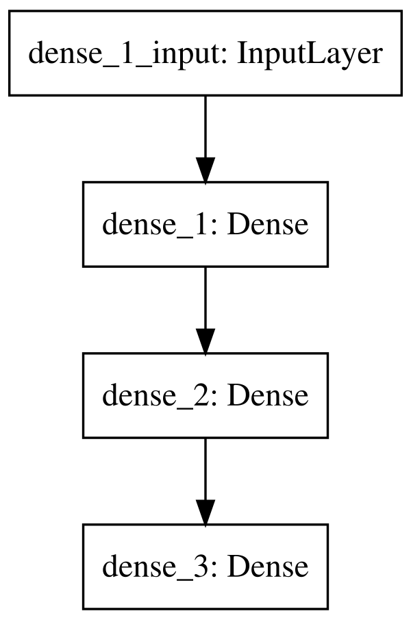
20.14 Visualizing Neural Networks
Problem
You want to quickly visualize a neural network’s architecture.
Solution
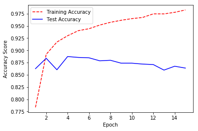
Use Keras’ model_to_dot or plot_model:
# Load librariesfromkerasimportmodelsfromkerasimportlayersfromIPython.displayimportSVGfromkeras.utils.vis_utilsimportmodel_to_dotfromkeras.utilsimportplot_model# Start neural networknetwork=models.Sequential()# Add fully connected layer with a ReLU activation functionnetwork.add(layers.Dense(units=16,activation="relu",input_shape=(10,)))# Add fully connected layer with a ReLU activation functionnetwork.add(layers.Dense(units=16,activation="relu"))# Add fully connected layer with a sigmoid activation functionnetwork.add(layers.Dense(units=1,activation="sigmoid"))# Visualize network architectureSVG(model_to_dot(network,show_shapes=True).create(prog="dot",format="svg"))
Using TensorFlow backend.
Alternatively, if we want to save the visualization as a file, we can
use plot_model:
# Save the visualization as a fileplot_model(network,show_shapes=True,to_file="network.png")
Discussion
Keras provides utility functions to quickly visualize neural networks.
If we wish to display a neural network in a Jupyter Notebook, we can use
model_to_dot. The show_shapes parameter shows the shape of the
inputs and outputs and can help with debugging. For a simpler model,
we can set show_shapes=True:
# Visualize network architectureSVG(model_to_dot(network,show_shapes=False).create(prog="dot",format="svg"))
20.15 Classifying Images
Solution
Use Keras to create a neural network with at least one convolutional layer:
importnumpyasnpfromkeras.datasetsimportmnistfromkeras.modelsimportSequentialfromkeras.layersimportDense,Dropout,Flattenfromkeras.layers.convolutionalimportConv2D,MaxPooling2Dfromkeras.utilsimportnp_utilsfromkerasimportbackendasK# Set that the color channel value will be firstK.set_image_data_format("channels_first")# Set seednp.random.seed(0)# Set image informationchannels=1height=28width=28# Load data and target from MNIST data(data_train,target_train),(data_test,target_test)=mnist.load_data()# Reshape training image data into featuresdata_train=data_train.reshape(data_train.shape[0],channels,height,width)# Reshape test image data into featuresdata_test=data_test.reshape(data_test.shape[0],channels,height,width)# Rescale pixel intensity to between 0 and 1features_train=data_train/255features_test=data_test/255# One-hot encode targettarget_train=np_utils.to_categorical(target_train)target_test=np_utils.to_categorical(target_test)number_of_classes=target_test.shape[1]# Start neural networknetwork=Sequential()# Add convolutional layer with 64 filters, a 5x5 window, and ReLU activation functionnetwork.add(Conv2D(filters=64,kernel_size=(5,5),input_shape=(channels,width,height),activation='relu'))# Add max pooling layer with a 2x2 windownetwork.add(MaxPooling2D(pool_size=(2,2)))# Add dropout layernetwork.add(Dropout(0.5))# Add layer to flatten inputnetwork.add(Flatten())# # Add fully connected layer of 128 units with a ReLU activation functionnetwork.add(Dense(128,activation="relu"))# Add dropout layernetwork.add(Dropout(0.5))# Add fully connected layer with a softmax activation functionnetwork.add(Dense(number_of_classes,activation="softmax"))# Compile neural networknetwork.compile(loss="categorical_crossentropy",# Cross-entropyoptimizer="rmsprop",# Root Mean Square Propagationmetrics=["accuracy"])# Accuracy performance metric# Train neural networknetwork.fit(features_train,# Featurestarget_train,# Targetepochs=2,# Number of epochsverbose=0,# Don't print description after each epochbatch_size=1000,# Number of observations per batchvalidation_data=(features_test,target_test))# Data for evaluation
Using TensorFlow backend.

<keras.callbacks.History at 0x133f37e80>
Discussion
Convolutional neural networks (also called ConvNets) are a popular type of network that has proven very effective at computer vision (e.g., recognizing cats, dogs, planes, and even hot dogs). It is completely possible to use feedforward neural networks on images, where each pixel is a feature. However, when doing so we run into two major problems. First, feedforward neural networks do not take into account the spatial structure of the pixels. For example, in a 10 × 10 pixel image we might convert it into a vector of 100 pixel features, and in this case feedforward would consider the first feature (e.g., pixel value) to have the same relationship with the 10th feature as the 11th feature. However, in reality the 10th feature represents a pixel on the far side of the image as the first feature, while the 11th feature represents the pixel immediately below the first pixel. Second, and relatedly, feedforward neural networks learn global relationships in the features instead of local patterns. In more practical terms, this means that feedforward neural networks are not able to detect an object regardless of where it appears in an image. For example, imagine we are training a neural network to recognize faces, and these faces might appear anywhere in the image from the upper right to the middle to the lower left.
The power of convolutional neural networks is their ability handle both of these issues (and others). A complete explanation of convolutional neural networks is well beyond the scope of this book, but a brief explanation will be useful. The data of an individual image contains two or three dimensions: height, width, and depth. The first two should be obvious, but the last deserves explanation. The depth is the color of a pixel. In grayscale images the depth is only one (the intensity of the pixel) and therefore the image is a matrix. However, in color images a pixel’s color is represented by multiple values. For example, in an RGB image a pixel’s color is represented by three values representing red, green, and blue. Therefore, the data for an image can be imagined to be a three-dimensional tensor: width × height × depth (called feature maps). In convolutional neural networks, a convolution (don’t worry if you don’t know what that means) can be imagined to slide a window over the pixels of an image, looking at both the individual pixel and also its neighbors. It then transforms the raw image data into a new three-dimensional tensor where the first two dimensions are approximately width and height, while the third dimension (which contained the color values) now represents the patterns—called filters—(for example, a sharp corner or sweeping gradient) to which that pixel “belongs.”
The second important concept for our purposes is that of pooling layers. Pooling layers move a window over our data (though usually they only look at every nth pixel, called striding) downsizing our data by summarizing the window in some way. The most common method is max pooling where the maximum value in each window is sent to the next layer. One reason for max pooling is merely practical; the convolutional process creates many more parameters to learn, which can get ungainly very quickly. Second, more intuitively, max pooling can be thought of as “zooming out” of an image.
An example might be useful here. Imagine we have an image containing a dog’s face. The first convolutional layer might find patterns like shape edges. Then we use a max pool layer to “zoom out,” and a second convolutional layer to find patterns like dog ears. Finally we use another max pooling layer to zoom out again and a final convolutional layer to find patterns like dogs’ faces.
Finally, fully connected layers are often used at the end of the network to do the actual classification.
While our solution might look like a lot of lines of code, it is actually very similar to our binary classifier from earlier in this chapter. In this solution we used the famous MNIST dataset, which is a de facto benchmark dataset in machine learning. The MNIST dataset contains 70,000 small images (28 × 28) of handwritten digits from 0 to 9. This dataset is labeled so that we know the actual digit (i.e., class) for each small image. The standard training-test split is to use 60,000 images for training and 10,000 for testing.
We reorganized the data into the format expected by a convolutional
network. Specifically, we used reshape to convert the observation data such that it is the shape Keras expects. Next, we rescaled the values to be between 0 and 1, since training performance can suffer if an observation’s values are much greater than the network’s parameters
(which are initialized as small numbers). Finally, we one-hot encoded
the target data so that every observation’s target has 10 classes,
representing the digits 0–9.
With the image data process we can build our convolutional network. First, we add a convolutional layer and specify the number of filters and other characteristics. The size of the window is a hyperparameter; however, 3 × 3 is standard practice for most images, while larger windows are often used in larger images. Second, we add a max pooling layer, summarizing the nearby pixels. Third, we add a dropout layer to reduce the chances of overfitting. Fourth, we add a flatten layer to convert the convolutionary inputs into a format able to be used by a fully connected layer. Finally, we add the fully connected layers and an output layer to do the actual classification. Notice that because this is a multiclass classification problem, we use the softmax activation function in the output layer.
It should be noted that this is a pretty simple convolutional neural network. It is common to see a much deeper network with many more convolutional and max pooling layers stacked together.
20.16 Improving Performance with Image Augmentation
Solution
For better results, preprocess the images and augment the data
beforehand using ImageDataGenerator:
# Load libraryfromkeras.preprocessing.imageimportImageDataGenerator# Create image augmentationaugmentation=ImageDataGenerator(featurewise_center=True,# Apply ZCA whiteningzoom_range=0.3,# Randomly zoom in on imageswidth_shift_range=0.2,# Randomly shift imageshorizontal_flip=True,# Randomly flip imagesrotation_range=90)# Randomly rotate# Process all images from the directory 'raw/images'augment_images=augmentation.flow_from_directory("raw/images",# Image folderbatch_size=32,# Batch sizeclass_mode="binary",# Classessave_to_dir="processed/images")
Using TensorFlow backend.


Found 12665 images belonging to 2 classes.
Discussion
First an apology—this solution’s code will not immediately run for you because you do not have the required folders of images. However, since the most common situation is having a directory of images, I wanted to include it. The technique should easily translate to your own images.
One way to improve the performance of a convolutional neural network is
to preprocess the images. We discussed a number of techniques in Chapter 8; however, it is worth noting that Keras’ ImageDataGenerator contains a number of basic preprocessing techniques. For example, in our solution we used featurewise_center=True to standardize the pixels across the entire data.
A second technique to improve performance is to add noise. An interesting feature of neural networks is that, counterintuitively, their performance often improves when noise is added to the data. The reason is that the additional noise can make the neural networks more robust in the face of real-world noise and prevents them from overfitting the data.
When training convolutional neural networks for images, we can add noise to our observations by randomly transforming images in various ways, such as flipping images or zooming in on images. Even small changes can significantly improve model performance. We can use the same ImageDataGenerator class to conduct these transformations. The Keras documentation (referenced in “See Also”) specifies the full list of available transformations; however, our example contains a sample of them are, including random zooming, shifting, flipping, and rotation.
It is important to note that the output of flow_from_directory is a Python generator object. This is because in most cases we will want to process the images on-demand as they are sent to the neural network for training. If we wanted to process all the images prior to training, we could simply iterate over the generator.
Finally, since augment_images is a generator, when training our neural
network we will have to use fit_generator instead of fit. For
example:
# Train neural networknetwork.fit_generator(augment_images,#Number of times to call the generator for each epochsteps_per_epoch=2000,# Number of epochsepochs=5,# Test data generatorvalidation_data=augment_images_test,# Number of items to call the generator# for each test epochvalidation_steps=800)
Note all the raw images used in this recipe are available on GitHub.
See Also
20.17 Classifying Text
Problem
You want to classify text data.
Solution
Use a long short-term memory recurrent neural network:
# Load librariesimportnumpyasnpfromkeras.datasetsimportimdbfromkeras.preprocessingimportsequencefromkerasimportmodelsfromkerasimportlayers# Set random seednp.random.seed(0)# Set the number of features we wantnumber_of_features=1000# Load data and target vector from movie review data(data_train,target_train),(data_test,target_test)=imdb.load_data(num_words=number_of_features)# Use padding or truncation to make each observation have 400 featuresfeatures_train=sequence.pad_sequences(data_train,maxlen=400)features_test=sequence.pad_sequences(data_test,maxlen=400)# Start neural networknetwork=models.Sequential()# Add an embedding layernetwork.add(layers.Embedding(input_dim=number_of_features,output_dim=128))# Add a long short-term memory layer with 128 unitsnetwork.add(layers.LSTM(units=128))# Add fully connected layer with a sigmoid activation functionnetwork.add(layers.Dense(units=1,activation="sigmoid"))# Compile neural networknetwork.compile(loss="binary_crossentropy",# Cross-entropyoptimizer="Adam",# Adam optimizationmetrics=["accuracy"])# Accuracy performance metric# Train neural networkhistory=network.fit(features_train,# Featurestarget_train,# Targetepochs=3,# Number of epochsverbose=0,# Do not print description after each epochbatch_size=1000,# Number of observations per batchvalidation_data=(features_test,target_test))# Test data
Using TensorFlow backend.
Discussion
Oftentimes we have text data that we want to classify. While it is possible to use a type of convolutional network, we are going to focus on a more popular option: the recurrent neural network. The key feature of recurrent neural networks is that information loops back in the network. This gives recurrent neural networks a type of memory they can use to better understand sequential data. A popular type of recurrent neural network is the long short-term memory (LSTM) network, which allows for information to loop backward in the network. For a more detailed explanation, see the additional resources.
In this solution, we have our movie review data from Recipe 20.3 and we want to train an LSTM network to predict if these reviews are positive or negative. Before we can train our network, a little data processing is needed. Our text data comes in the form of a list of integers:
# View first observation(data_train[0])
[1, 14, 22, 16, 43, 530, 973, 2, 2, 65, 458, 2, 66, 2, 4, 173, 36, 256, 5, 25,
    100, 43, 838, 112, 50, 670, 2, 9, 35, 480, 284, 5, 150, 4, 172, 112, 167, 2,
    336, 385, 39, 4, 172, 2, 2, 17, 546, 38, 13, 447, 4, 192, 50, 16, 6, 147, 2,
    19, 14, 22, 4, 2, 2, 469, 4, 22, 71, 87, 12, 16, 43, 530, 38, 76, 15, 13, 2,
    4, 22, 17, 515, 17, 12, 16, 626, 18, 2, 5, 62, 386, 12, 8, 316, 8, 106, 5, 4,
    2, 2, 16, 480, 66, 2, 33, 4, 130, 12, 16, 38, 619, 5, 25, 124, 51, 36, 135,
    48, 25, 2, 33, 6, 22, 12, 215, 28, 77, 52, 5, 14, 407, 16, 82, 2, 8, 4, 107,
    117, 2, 15, 256, 4, 2, 7, 2, 5, 723, 36, 71, 43, 530, 476, 26, 400, 317, 46,
    7, 4, 2, 2, 13, 104, 88, 4, 381, 15, 297, 98, 32, 2, 56, 26, 141, 6, 194, 2,
    18, 4, 226, 22, 21, 134, 476, 26, 480, 5, 144, 30, 2, 18, 51, 36, 28, 224,
    92, 25, 104, 4, 226, 65, 16, 38, 2, 88, 12, 16, 283, 5, 16, 2, 113, 103, 32,
    15, 16, 2, 19, 178, 32]
Each integer in this list corresponds to some word. However, because
each review does not contain the same number of words, each observation
is not the same length. Therefore, before we can input this data into
our neural network, we need to make all the observations the same
length. We can do this using pad_sequences. pad_sequences pads each observation’s data so that they are all the same size. We can see this if we look at our first observation after it is processed by pad_sequences:
# View first observation(features_test[0])
[  0   0   0   0   0   0   0   0   0   0   0   0   0   0   0   0   0   0
   0   0   0   0   0   0   0   0   0   0   0   0   0   0   0   0   0   0
   0   0   0   0   0   0   0   0   0   0   0   0   0   0   0   0   0   0
   0   0   0   0   0   0   0   0   0   0   0   0   0   0   0   0   0   0
   0   0   0   0   0   0   0   0   0   0   0   0   0   0   0   0   0   0
   0   0   0   0   0   0   0   0   0   0   0   0   0   0   0   0   0   0
   0   0   0   0   0   0   0   0   0   0   0   0   0   0   0   0   0   0
   0   0   0   0   0   0   0   0   0   0   0   0   0   0   0   0   0   0
   0   0   0   0   0   0   0   0   0   0   0   0   0   0   0   0   0   0
   0   0   0   0   0   0   0   0   0   0   0   0   0   0   0   0   0   0
   0   0   0   0   0   0   0   0   0   0   0   0   0   0   0   0   0   0
   0   0   0   0   0   0   0   0   0   0   0   0   0   0   0   0   0   0
   0   0   0   0   0   0   0   0   0   0   0   0   0   0   0   0   0   0
   0   0   0   0   0   0   0   0   0   0   0   0   0   0   0   0   0   0
   0   0   0   0   0   0   0   0   0   0   0   0   0   0   0   0   0   0
   0   0   0   0   0   0   0   0   0   0   0   0   0   0   0   0   0   0
   0   0   0   0   0   0   0   0   0   0   0   0   0   0   0   0   0   0
   0   0   0   0   0   0   0   0   0   0   0   0   0   0   0   0   0   0
   0   0   0   0   1  89  27   2   2  17 199 132   5   2  16   2  24   8
 760   4   2   7   4  22   2   2  16   2  17   2   7   2   2   9   4   2
   8  14 991  13 877  38  19  27 239  13 100 235  61 483   2   4   7   4
  20 131   2  72   8  14 251  27   2   7 308  16 735   2  17  29 144  28
  77   2  18  12]
Next, we use one of the most promising techniques in natural language
processing: word embeddings. In our binary classifier from Recipe 20.3, we one-hot encoded the observations and used that as inputs to the neural network. However, this time we will represent each word as a vector in a multidimensional space, and allow the distance between two vectors to represent the similarity between words. In Keras we can do this by adding an Embedding layer. For each value sent to the Embedding layer, it will output a vector representing that word. The following layer is our LSTM layer with 128 units, which allows for information from earlier inputs to be used in futures, directly addressing the sequential nature of the data. Finally, because this is a binary classification problem (each review is positive or negative), we add a fully connected output layer with one unit and a sigmoid activation function.
It is worth noting that LSTMs are a very broad topic and the focus of much research. This recipe, while hopefully useful, is far from the last word on the implementation of LSTMs.