Table of Contents for
Machine Learning with Python Cookbook
 Machine Learning with Python Cookbook
Published by
O'Reilly Media, Inc., 2018
Machine Learning with Python Cookbook
Published by
O'Reilly Media, Inc., 2018
- Cover
- nav
- Machine Learning with Python Cookbook
- Machine Learning with Python Cookbook
- Preface
- Vectors, Matrices, and Arrays
- Loading Data
- Data Wrangling
- Handling Numerical Data
- Handling Categorical Data
- Handling Text
- Handling Dates and Times
- Handling Images
- Dimensionality Reduction Using Feature Extraction
- Dimensionality Reduction Using Feature Selection
- Model Evaluation
- Model Selection
- Linear Regression
- Trees and Forests
- K-Nearest Neighbors
- Logistic Regression
- Support Vector Machines
- Naive Bayes
- Clustering
- Neural Networks
- Saving and Loading Trained Models
- Index
- About the Author
- Colophon
Chapter 8. Handling Images
8.0 Introduction
Image classification is one of the most exciting areas of machine learning. The ability of computers to recognize patterns and objects from images is an incredibly powerful tool in our toolkit. However, before we can apply machine learning to images, we often first need to transform the raw images to features usable by our learning algorithms.
To work with images, we will use the Open Source Computer Vision Library (OpenCV). While there are a number of good libraries out there, OpenCV is the most popular and documented library for handling images. One of the biggest hurdles to using OpenCV is installing it. However, fortunately if we are using Python 3 (at the time of publication OpenCV does not work with Python 3.6+), we can use Anaconda’s package manager tool conda to install OpenCV in a single line of code in our terminal:
conda install --channel https://conda.anaconda.org/menpo opencv3
Afterward, we can check the installation by opening a notebook, importing OpenCV, and checking the version number (3.1.0):
import cv2

cv2.__version__
If installing OpenCV using conda does not work, there are many guides online.
Finally, throughout this chapter we will use a set of images as examples, which are available to download on GitHub.
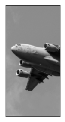
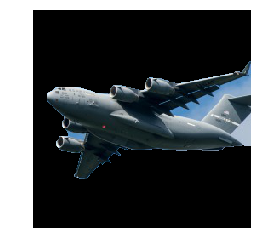
8.1 Loading Images
Solution
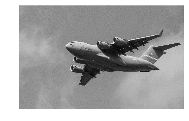
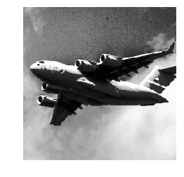
# Load libraryimportcv2importnumpyasnpfrommatplotlibimportpyplotasplt# Load image as grayscaleimage=cv2.imread("images/plane.jpg",cv2.IMREAD_GRAYSCALE)
If we want to view the image, we can use the Python plotting library Matplotlib:
# Show imageplt.imshow(image,cmap="gray"),plt.axis("off")plt.show()
Discussion
Fundamentally, images are data and when we use imread we convert that
data into a data type we are very familiar with—a NumPy array:
# Show data typetype(image)
numpy.ndarray
We have transformed the image into a matrix whose elements correspond to individual pixels. We can even take a look at the actual values of the matrix:
# Show image dataimage
array([[140, 136, 146, ..., 132, 139, 134],
       [144, 136, 149, ..., 142, 124, 126],
       [152, 139, 144, ..., 121, 127, 134],
       ...,
       [156, 146, 144, ..., 157, 154, 151],
       [146, 150, 147, ..., 156, 158, 157],
       [143, 138, 147, ..., 156, 157, 157]], dtype=uint8)
The resolution of our image was 3600 × 2270, the exact dimensions of our matrix:
# Show dimensionsimage.shape
(2270, 3600)
What does each element in the matrix actually represent? In grayscale images, the value of an individual element is the pixel intensity. Intensity values range from black (0) to white (255). For example, the intensity of the top-rightmost pixel in our image has a value of 140:
# Show first pixelimage[0,0]
140
In the matrix, each element contains three values corresponding to blue, green, red values (BGR):
# Load image in colorimage_bgr=cv2.imread("images/plane.jpg",cv2.IMREAD_COLOR)# Show pixelimage_bgr[0,0]
array([195, 144, 111], dtype=uint8)
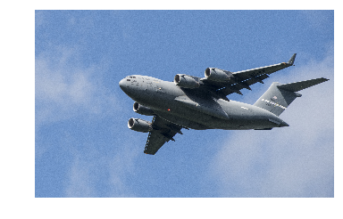
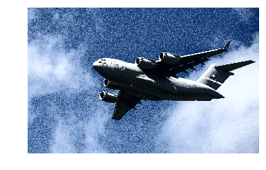
One small caveat: by default OpenCV uses BGR, but many image applications—including Matplotlib—use red, green, blue (RGB), meaning the red and the blue values are swapped. To properly display OpenCV color images in Matplotlib, we need to first convert the color to RGB (apologies to hardcopy readers):
# Convert to RGBimage_rgb=cv2.cvtColor(image_bgr,cv2.COLOR_BGR2RGB)# Show imageplt.imshow(image_rgb),plt.axis("off")plt.show()
8.2 Saving Images
Discussion
OpenCV’s imwrite saves images to the filepath specified. The format
of the image is defined by the filename’s extension (.jpg,
.png, etc.). One behavior to be careful about: imwrite will
overwrite existing files without outputting an error or asking for
confirmation.
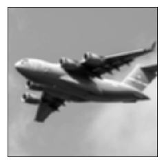
8.3 Resizing Images
Solution
Use resize to change the size of an image:
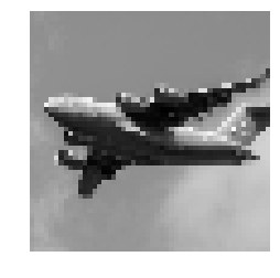
# Load imageimportcv2importnumpyasnpfrommatplotlibimportpyplotasplt# Load image as grayscaleimage=cv2.imread("images/plane_256x256.jpg",cv2.IMREAD_GRAYSCALE)# Resize image to 50 pixels by 50 pixelsimage_50x50=cv2.resize(image,(50,50))# View imageplt.imshow(image_50x50,cmap="gray"),plt.axis("off")plt.show()
Discussion
Resizing images is a common task in image preprocessing for two reasons. First, images come in all shapes and sizes, and to be usable as features, images must have the same dimensions. This standardization of image size does come with costs, however; images are matrices of information and when we reduce the size of the image we are reducing the size of that matrix and the information it contains. Second, machine learning can require thousands or hundreds of thousands of images. When those images are very large they can take up a lot of memory, and by resizing them we can dramatically reduce memory usage. Some common image sizes for machine learning are 32 × 32, 64 × 64, 96 × 96, and 256 × 256.
8.4 Cropping Images
Solution
The image is encoded as a two-dimensional NumPy array, so we can crop the image easily by slicing the array:
# Load imageimportcv2importnumpyasnpfrommatplotlibimportpyplotasplt# Load image in grayscaleimage=cv2.imread("images/plane_256x256.jpg",cv2.IMREAD_GRAYSCALE)# Select first half of the columns and all rowsimage_cropped=image[:,:128]# Show imageplt.imshow(image_cropped,cmap="gray"),plt.axis("off")plt.show()
Discussion
Since OpenCV represents images as a matrix of elements, by selecting the rows and columns we want to keep we are able to easily crop the image. Cropping can be particularly useful if we know that we only want to keep a certain part of every image. For example, if our images come from a stationary security camera we can crop all the images so they only contain the area of interest.
See Also
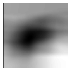
8.5 Blurring Images
Solution
To blur an image, each pixel is transformed to be the average value of its neighbors. This neighbor and the operation performed are mathematically represented as a kernel (don’t worry if you don’t know what a kernel is). The size of this kernel determines the amount of blurring, with larger kernels producing smoother images. Here we blur an image by averaging the values of a 5 × 5 kernel around each pixel:
# Load librariesimportcv2importnumpyasnpfrommatplotlibimportpyplotasplt# Load image as grayscaleimage=cv2.imread("images/plane_256x256.jpg",cv2.IMREAD_GRAYSCALE)# Blur imageimage_blurry=cv2.blur(image,(5,5))# Show imageplt.imshow(image_blurry,cmap="gray"),plt.axis("off")plt.show()
To highlight the effect of kernel size, here is the same blurring with a 100 × 100 kernel:
# Blur imageimage_very_blurry=cv2.blur(image,(100,100))# Show imageplt.imshow(image_very_blurry,cmap="gray"),plt.xticks([]),plt.yticks([])plt.show()
Discussion
Kernels are widely used in image processing to do everything from sharpening to edge detection, and will come up repeatedly in this chapter. The blurring kernel we used looks like this:
# Create kernelkernel=np.ones((5,5))/25.0# Show kernelkernel
array([[ 0.04,  0.04,  0.04,  0.04,  0.04],
       [ 0.04,  0.04,  0.04,  0.04,  0.04],
       [ 0.04,  0.04,  0.04,  0.04,  0.04],
       [ 0.04,  0.04,  0.04,  0.04,  0.04],
       [ 0.04,  0.04,  0.04,  0.04,  0.04]])
The center element in the kernel is the pixel being examined, while the
remaining elements are its neighbors. Since all elements have the same
value (normalized to add up to 1), each has an equal say in the
resulting value of the pixel of interest. We can manually apply a kernel
to an image using filter2D to produce a similar blurring effect:
# Apply kernelimage_kernel=cv2.filter2D(image,-1,kernel)# Show imageplt.imshow(image_kernel,cmap="gray"),plt.xticks([]),plt.yticks([])plt.show()

8.6 Sharpening Images
Solution
Create a kernel that highlights the target pixel. Then apply it to the
image using filter2D:
# Load librariesimportcv2importnumpyasnpfrommatplotlibimportpyplotasplt# Load image as grayscaleimage=cv2.imread("images/plane_256x256.jpg",cv2.IMREAD_GRAYSCALE)# Create kernelkernel=np.array([[0,-1,0],[-1,5,-1],[0,-1,0]])# Sharpen imageimage_sharp=cv2.filter2D(image,-1,kernel)# Show imageplt.imshow(image_sharp,cmap="gray"),plt.axis("off")plt.show()
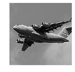
8.7 Enhancing Contrast
Solution
Histogram equalization is a tool for image processing that can make
objects and shapes stand out. When we have a grayscale image, we can
apply OpenCV’s equalizeHist directly on the image:
# Load librariesimportcv2importnumpyasnpfrommatplotlibimportpyplotasplt# Load imageimage=cv2.imread("images/plane_256x256.jpg",cv2.IMREAD_GRAYSCALE)# Enhance imageimage_enhanced=cv2.equalizeHist(image)# Show imageplt.imshow(image_enhanced,cmap="gray"),plt.axis("off")plt.show()
However, when we have a color image, we first need to convert the image
to the YUV color format. The Y is the luma, or brightness, and U and V
denote the color. After the conversion, we can apply equalizeHist to
the image and then convert it back to BGR or RGB:
# Load imageimage_bgr=cv2.imread("images/plane.jpg")# Convert to YUVimage_yuv=cv2.cvtColor(image_bgr,cv2.COLOR_BGR2YUV)# Apply histogram equalizationimage_yuv[:,:,0]=cv2.equalizeHist(image_yuv[:,:,0])# Convert to RGBimage_rgb=cv2.cvtColor(image_yuv,cv2.COLOR_YUV2RGB)# Show imageplt.imshow(image_rgb),plt.axis("off")plt.show()
Discussion
While a detailed explanation of how histogram equalization works is beyond the scope of this book, the short explanation is that it transforms the image so that it uses a wider range of pixel intensities.
While the resulting image often does not look “realistic,” we need to remember that the image is just a visual representation of the underlying data. If histogram equalization is able to make objects of interest more distinguishable from other objects or backgrounds (which is not always the case), then it can be a valuable addition to our image preprocessing pipeline.
8.8 Isolating Colors
Solution
Define a range of colors and then apply a mask to the image:
# Load librariesimportcv2importnumpyasnpfrommatplotlibimportpyplotasplt# Load imageimage_bgr=cv2.imread('images/plane_256x256.jpg')# Convert BGR to HSVimage_hsv=cv2.cvtColor(image_bgr,cv2.COLOR_BGR2HSV)# Define range of blue values in HSVlower_blue=np.array([50,100,50])upper_blue=np.array([130,255,255])# Create maskmask=cv2.inRange(image_hsv,lower_blue,upper_blue)# Mask imageimage_bgr_masked=cv2.bitwise_and(image_bgr,image_bgr,mask=mask)# Convert BGR to RGBimage_rgb=cv2.cvtColor(image_bgr_masked,cv2.COLOR_BGR2RGB)# Show imageplt.imshow(image_rgb),plt.axis("off")plt.show()
Discussion
Isolating colors in OpenCV is straightforward. First we convert an image into HSV (hue, saturation, and value). Second, we define a range of values we want to isolate, which is probably the most difficult and time-consuming part. Third, we create a mask for the image (we will only keep the white areas):
# Show imageplt.imshow(mask,cmap='gray'),plt.axis("off")plt.show()
Finally, we apply the mask to the image using bitwise_and and convert
to our desired output format.
8.9 Binarizing Images
Solution
Thresholding is the process of setting pixels with intensity greater than some value to be white and less than the value to be black. A more advanced technique is adaptive thresholding, where the threshold value for a pixel is determined by the pixel intensities of its neighbors. This can be helpful when lighting conditions change over different regions in an image:
# Load librariesimportcv2importnumpyasnpfrommatplotlibimportpyplotasplt# Load image as grayscaleimage_grey=cv2.imread("images/plane_256x256.jpg",cv2.IMREAD_GRAYSCALE)# Apply adaptive thresholdingmax_output_value=255neighborhood_size=99subtract_from_mean=10image_binarized=cv2.adaptiveThreshold(image_grey,max_output_value,cv2.ADAPTIVE_THRESH_GAUSSIAN_C,cv2.THRESH_BINARY,neighborhood_size,subtract_from_mean)# Show imageplt.imshow(image_binarized,cmap="gray"),plt.axis("off")plt.show()

Discussion
Our solution has four important arguments in adaptiveThreshold.
max_output_value simply determines the maximum intensity of the output
pixel intensities. cv2.ADAPTIVE_THRESH_GAUSSIAN_C sets a pixel’s
threshold to be a weighted sum of the neighboring pixel intensities. The
weights are determined by a Gaussian window. Alternatively we could set
the threshold to simply the mean of the neighboring pixels with
cv2.ADAPTIVE_THRESH_MEAN_C:
# Apply cv2.ADAPTIVE_THRESH_MEAN_Cimage_mean_threshold=cv2.adaptiveThreshold(image_grey,max_output_value,cv2.ADAPTIVE_THRESH_MEAN_C,cv2.THRESH_BINARY,neighborhood_size,subtract_from_mean)# Show imageplt.imshow(image_mean_threshold,cmap="gray"),plt.axis("off")plt.show()
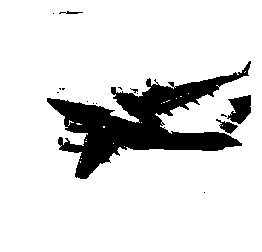
The last two parameters are the block size (the size of the neighborhood used to determine a pixel’s threshold) and a constant subtracted from the calculated threshold (used to manually fine-tune the threshold).
A major benefit of thresholding is denoising an image—keeping only the most important elements. For example, thresholding is often applied to photos of printed text to isolate the letters from the page.
8.10 Removing Backgrounds
Solution
Mark a rectangle around the desired foreground, then run the GrabCut algorithm:
# Load libraryimportcv2importnumpyasnpfrommatplotlibimportpyplotasplt# Load image and convert to RGBimage_bgr=cv2.imread('images/plane_256x256.jpg')image_rgb=cv2.cvtColor(image_bgr,cv2.COLOR_BGR2RGB)# Rectangle values: start x, start y, width, heightrectangle=(0,56,256,150)# Create initial maskmask=np.zeros(image_rgb.shape[:2],np.uint8)# Create temporary arrays used by grabCutbgdModel=np.zeros((1,65),np.float64)fgdModel=np.zeros((1,65),np.float64)# Run grabCutcv2.grabCut(image_rgb,# Our imagemask,# The Maskrectangle,# Our rectanglebgdModel,# Temporary array for backgroundfgdModel,# Temporary array for background5,# Number of iterationscv2.GC_INIT_WITH_RECT)# Initiative using our rectangle# Create mask where sure and likely backgrounds set to 0, otherwise 1mask_2=np.where((mask==2)|(mask==0),0,1).astype('uint8')# Multiply image with new mask to subtract backgroundimage_rgb_nobg=image_rgb*mask_2[:,:,np.newaxis]# Show imageplt.imshow(image_rgb_nobg),plt.axis("off")plt.show()
Discussion
The first thing we notice is that even though GrabCut did a pretty good job, there are still areas of background left in the image. We could go back and manually mark those areas as background, but in the real world we have thousands of images and manually fixing them individually is not feasible. Therefore, we would do well by simply accepting that the image data will still contain some background noise.
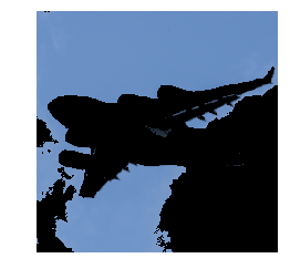
In our solution, we start out by marking a rectangle around the area that contains the foreground. GrabCut assumes everything outside this rectangle to be background and uses that information to figure out what is likely background inside the square (to learn how the algorithm does this, check out the external resources at the end of this solution). Then a mask is created that denotes the different definitely/likely background/foreground regions:
# Show maskplt.imshow(mask,cmap='gray'),plt.axis("off")plt.show()

The black region is the area outside our rectangle that is assumed to be definitely background. The gray area is what GrabCut considered likely background, while the white area is likely foreground.
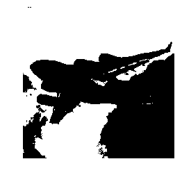
This mask is then used to create a second mask that merges the black and gray regions:
# Show maskplt.imshow(mask_2,cmap='gray'),plt.axis("off")plt.show()

The second mask is then applied to the image so that only the foreground remains.
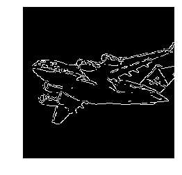
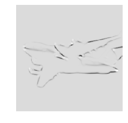
8.11 Detecting Edges
Solution
Use an edge detection technique like the Canny edge detector:
# Load libraryimportcv2importnumpyasnpfrommatplotlibimportpyplotasplt# Load image as grayscaleimage_gray=cv2.imread("images/plane_256x256.jpg",cv2.IMREAD_GRAYSCALE)# Calculate median intensitymedian_intensity=np.median(image_gray)# Set thresholds to be one standard deviation above and below median intensitylower_threshold=int(max(0,(1.0-0.33)*median_intensity))upper_threshold=int(min(255,(1.0+0.33)*median_intensity))# Apply canny edge detectorimage_canny=cv2.Canny(image_gray,lower_threshold,upper_threshold)# Show imageplt.imshow(image_canny,cmap="gray"),plt.axis("off")plt.show()
Discussion
Edge detection is a major topic of interest in computer vision. Edges are important because they are areas of high information. For example, in our image one patch of sky looks very much like another and is unlikely to contain unique or interesting information. However, patches where the background sky meets the airplane contain a lot of information (e.g., an object’s shape). Edge detection allows us to remove low-information areas and isolate the areas of images containing the most information.
There are many edge detection techniques (Sobel filters, Laplacian edge detector, etc.). However, our solution uses the commonly used Canny edge detector. How the Canny detector works is too detailed for this book, but there is one point that we need to address. The Canny detector requires two parameters denoting low and high gradient threshold values. Potential edge pixels between the low and high thresholds are considered weak edge pixels, while those above the high threshold are considered strong edge pixels. OpenCV’s Canny method includes the low and high thresholds as required parameters. In our solution, we set the lower and upper thresholds to be one standard deviation below and above the image’s median pixel intensity. However, there are often cases when we might get better results if we used a good pair of low and high threshold values through manual trial and error using a few images before running Canny on our entire collection of images.
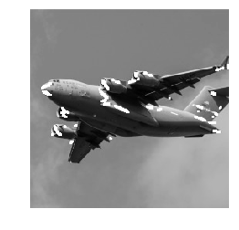
8.12 Detecting Corners
Solution
Use OpenCV’s implementation of the Harris corner detector,
cornerHarris:
# Load librariesimportcv2importnumpyasnpfrommatplotlibimportpyplotasplt# Load image as grayscaleimage_bgr=cv2.imread("images/plane_256x256.jpg")image_gray=cv2.cvtColor(image_bgr,cv2.COLOR_BGR2GRAY)image_gray=np.float32(image_gray)# Set corner detector parametersblock_size=2aperture=29free_parameter=0.04# Detect cornersdetector_responses=cv2.cornerHarris(image_gray,block_size,aperture,free_parameter)# Large corner markersdetector_responses=cv2.dilate(detector_responses,None)# Only keep detector responses greater than threshold, mark as whitethreshold=0.02image_bgr[detector_responses>threshold*detector_responses.max()]=[255,255,255]# Convert to grayscaleimage_gray=cv2.cvtColor(image_bgr,cv2.COLOR_BGR2GRAY)# Show imageplt.imshow(image_gray,cmap="gray"),plt.axis("off")plt.show()
Discussion
The Harris corner detector is a commonly used method of detecting the
intersection of two edges. Our interest in detecting corners is
motivated by the same reason as for deleting edges: corners are
points of high information. A complete explanation of the Harris corner detector is available in the external resources at the end of this recipe, but a simplified explanation is that it looks for windows (also called neighborhoods or patches) where small movements of the window (imagine shaking the window) creates big changes in the contents of the pixels inside the window. cornerHarris contains three important parameters that we can use to control the edges detected. First, block_size is the size of the neighbor around each pixel used for corner detection. Second, aperture is the size of the Sobel kernel used (don’t worry if you don’t know what that is), and finally there is a free parameter where larger values correspond to identifying softer corners.
The output is a grayscale image depicting potential corners:
# Show potential cornersplt.imshow(detector_responses,cmap='gray'),plt.axis("off")plt.show()
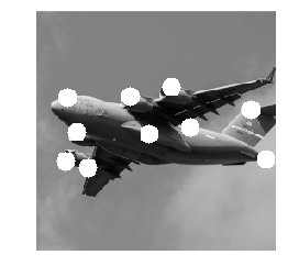
We then apply thresholding to keep only the most likely corners. Alternatively, we can use a similar detector, the Shi-Tomasi corner detector, which works in a similar way to the Harris detector (goodFeaturesToTrack) to identify a fixed number of strong corners. goodFeaturesToTrack takes three major parameters—the number of corners to detect, the minimum quality of the corner (0 to 1), and the minimum Euclidean distance between corners:
# Load imagesimage_bgr=cv2.imread('images/plane_256x256.jpg')image_gray=cv2.cvtColor(image_bgr,cv2.COLOR_BGR2GRAY)# Number of corners to detectcorners_to_detect=10minimum_quality_score=0.05minimum_distance=25# Detect cornerscorners=cv2.goodFeaturesToTrack(image_gray,corners_to_detect,minimum_quality_score,minimum_distance)corners=np.float32(corners)# Draw white circle at each cornerforcornerincorners:x,y=corner[0]cv2.circle(image_bgr,(x,y),10,(255,255,255),-1)# Convert to grayscaleimage_rgb=cv2.cvtColor(image_bgr,cv2.COLOR_BGR2GRAY)# Show imageplt.imshow(image_rgb,cmap='gray'),plt.axis("off")plt.show()
8.13 Creating Features for Machine Learning
Solution
Use NumPy’s flatten to convert the multidimensional array containing
an image’s data into a vector containing the observation’s values:
# Load imageimportcv2importnumpyasnpfrommatplotlibimportpyplotasplt# Load image as grayscaleimage=cv2.imread("images/plane_256x256.jpg",cv2.IMREAD_GRAYSCALE)# Resize image to 10 pixels by 10 pixelsimage_10x10=cv2.resize(image,(10,10))# Convert image data to one-dimensional vectorimage_10x10.flatten()
array([133, 130, 130, 129, 130, 129, 129, 128, 128, 127, 135, 131, 131,
       131, 130, 130, 129, 128, 128, 128, 134, 132, 131, 131, 130, 129,
       129, 128, 130, 133, 132, 158, 130, 133, 130,  46,  97,  26, 132,
       143, 141,  36,  54,  91,   9,   9,  49, 144, 179,  41, 142,  95,
        32,  36,  29,  43, 113, 141, 179, 187, 141, 124,  26,  25, 132,
       135, 151, 175, 174, 184, 143, 151,  38, 133, 134, 139, 174, 177,
       169, 174, 155, 141, 135, 137, 137, 152, 169, 168, 168, 179, 152,
       139, 136, 135, 137, 143, 159, 166, 171, 175], dtype=uint8)
Discussion
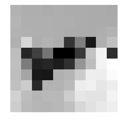
Images are presented as a grid of pixels. If an image is in grayscale,
each pixel is presented by one value (i.e., pixel intensity: 1 if
white, 0 if black). For example, imagine we have a 10 × 10–pixel
image:
plt.imshow(image_10x10,cmap="gray"),plt.axis("off")plt.show()
In this case the dimensions of the images data will be 10 × 10:
image_10x10.shape
(10, 10)
And if we flatten the array, we get a vector of length 100 (10 multiplied by 10):
image_10x10.flatten().shape
(100,)
This is the feature data for our image that can be joined with the vectors from other images to create the data we will feed to our machine learning algorithms.
If the image is in color, instead of each pixel being represented by one value, it is represented by multiple values (most often three) representing the channels (red, green, blue, etc.) that blend to make the final color of that pixel. For this reason, if our 10 × 10 image is in color, we will have 300 feature values for each observation:
# Load image in colorimage_color=cv2.imread("images/plane_256x256.jpg",cv2.IMREAD_COLOR)# Resize image to 10 pixels by 10 pixelsimage_color_10x10=cv2.resize(image_color,(10,10))# Convert image data to one-dimensional vector, show dimensionsimage_color_10x10.flatten().shape
(300,)
One of the major challenges of image processing and computer vision is that since every pixel location in a collection of images is a feature, as the images get larger, the number of features explodes:
# Load image in grayscaleimage_256x256_gray=cv2.imread("images/plane_256x256.jpg",cv2.IMREAD_GRAYSCALE)# Convert image data to one-dimensional vector, show dimensionsimage_256x256_gray.flatten().shape
(65536,)
And the number of features only intensifies when the image is in color:
# Load image in colorimage_256x256_color=cv2.imread("images/plane_256x256.jpg",cv2.IMREAD_COLOR)# Convert image data to one-dimensional vector, show dimensionsimage_256x256_color.flatten().shape
(196608,)
As the output shows, even a small color image has almost 200,000 features, which can cause problems when we are training our models because the number of features might far exceed the number of observations.
This problem will motivate dimensionality strategies discussed in a later chapter, which attempt to reduce the number of features while not losing an excessive amount of information contained in the data.
8.14 Encoding Mean Color as a Feature
Solution
Each pixel in an image is represented by the combination of multiple color channels (often three: red, green, and blue). Calculate the mean red, green, and blue channel values for an image to make three color features representing the average colors in that image:
# Load librariesimportcv2importnumpyasnpfrommatplotlibimportpyplotasplt# Load image as BGRimage_bgr=cv2.imread("images/plane_256x256.jpg",cv2.IMREAD_COLOR)# Calculate the mean of each channelchannels=cv2.mean(image_bgr)# Swap blue and red values (making it RGB, not BGR)observation=np.array([(channels[2],channels[1],channels[0])])# Show mean channel valuesobservation
array([[ 90.53204346, 133.11735535, 169.03074646]])
We can view the mean channel values directly (apologies to printed book readers):
# Show imageplt.imshow(observation),plt.axis("off")plt.show()

Discussion
The output is three feature values for an observation, one for each color channel in the image. These features can be used like any other features in learning algorithms to classify images according to their colors.
8.15 Encoding Color Histograms as Features
Solution
Compute the histograms for each color channel:
# Load librariesimportcv2importnumpyasnpfrommatplotlibimportpyplotasplt# Load imageimage_bgr=cv2.imread("images/plane_256x256.jpg",cv2.IMREAD_COLOR)# Convert to RGBimage_rgb=cv2.cvtColor(image_bgr,cv2.COLOR_BGR2RGB)# Create a list for feature valuesfeatures=[]# Calculate the histogram for each color channelcolors=("r","g","b")# For each channel: calculate histogram and add to feature value listfori,channelinenumerate(colors):histogram=cv2.calcHist([image_rgb],# Image[i],# Index of channelNone,# No mask[256],# Histogram size[0,256])# Rangefeatures.extend(histogram)# Create a vector for an observation's feature valuesobservation=np.array(features).flatten()# Show the observation's value for the first five featuresobservation[0:5]
array([ 1008., 217., 184., 165., 116.], dtype=float32)
Discussion
In the RGB color model, each color is the combination of three color channels (i.e., red, green, blue). In turn, each channel can take on one of 256 values (represented by an integer between 0 and 255). For example, the top-leftmost pixel in our image has the following channel values:
# Show RGB channel valuesimage_rgb[0,0]
array([107, 163, 212], dtype=uint8)
A histogram is a representation of the distribution of values in data. Here is a simple example:
# Import pandasimportpandasaspd# Create some datadata=pd.Series([1,1,2,2,3,3,3,4,5])# Show the histogramdata.hist(grid=False)plt.show()
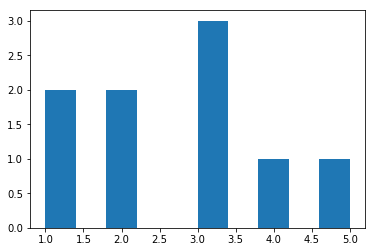
In this example, we have some data with two 1s, two 2s, three
3s, one 4, and one 5. In the histogram, each bar represents the number of times each value (1, 2, etc.) appears in our data.
We can apply this same technique to each of the color channels, but instead of five possible values, we have 256 (the range of possible values for a channel value). The x-axis represents the 256 possible channel values, and the y-axis represents the number of times a particular channel value appears across all pixels in an image:
# Calculate the histogram for each color channelcolors=("r","g","b")# For each channel: calculate histogram, make plotfori,channelinenumerate(colors):histogram=cv2.calcHist([image_rgb],# Image[i],# Index of channelNone,# No mask[256],# Histogram size[0,256])# Rangeplt.plot(histogram,color=channel)plt.xlim([0,256])# Show plotplt.show()
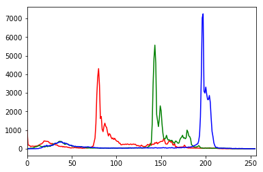
As we can see in the histogram, barely any pixels contain the blue channel values between 0 and ~180, while many pixels contain blue channel values between ~190 and ~210. This distribution of channel values is shown for all three channels. The histogram, however, is not simply a visualization; it is 256 features for each color channel, making for 768 total features representing the distribution of colors in an image.