Problem

You need to train a model to classify observations.

Solution

Use a support vector classifier (SVC) to find the hyperplane that maximizes the margins between the classes:

# Load libraries
from sklearn.svm import LinearSVC
from sklearn import datasets
from sklearn.preprocessing import StandardScaler
import numpy as np

# Load data with only two classes and two features
iris = datasets.load_iris()
features = iris.data[:100,:2]
target = iris.target[:100]

# Standardize features
scaler = StandardScaler()
features_standardized = scaler.fit_transform(features)

# Create support vector classifier
svc = LinearSVC(C=1.0)

# Train model
model = svc.fit(features_standardized, target)

Discussion

scikit-learn’s LinearSVC implements a simple SVC. To get an intuition behind what an SVC is doing, let us plot out the data and hyperplane. While SVCs work well in high dimensions, in our solution we only loaded two features and took a subset of observations so that the data contains only two classes. This will let us visualize the model. Recall that SVC attempts to find the hyperplane—a line when we only have two dimensions—with the maximum margin between the classes. In the following code we plot the two classes on a two-dimensional space, then draw the hyperplane:

# Load library
from matplotlib import pyplot as plt

# Plot data points and color using their class
color = ["black" if c == 0 else "lightgrey" for c in target]
plt.scatter(features_standardized[:,0], features_standardized[:,1], c=color)

# Create the hyperplane
w = svc.coef_[0]
a = -w[0] / w[1]
xx = np.linspace(-2.5, 2.5)
yy = a * xx - (svc.intercept_[0]) / w[1]

# Plot the hyperplane
plt.plot(xx, yy)
plt.axis("off"), plt.show();

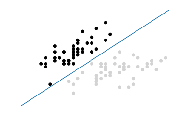
In this visualization, all observations of class 0 are black and observations of class 1 are light gray. The hyperplane is the decision boundary deciding how new observations are classified. Specifically, any observation above the line will by classified as class 0 while any observation below the line will be classified as class 1. We can prove this by creating a new observation in the top-left corner of our visualization, meaning it should be predicted to be class 0:

# Create new observation
new_observation = [[ -2,  3]]

# Predict class of new observation
svc.predict(new_observation)

array([0])

There are a few things to note about SVCs. First, for the sake of visualization we limited our example to a binary example (e.g., only two classes); however, SVCs can work well with multiple classes. Second, as our visualization shows, the hyperplane is by definition linear (i.e., not curved). This was okay in this example because the data was linearly separable, meaning there was a hyperplane that could perfectly separate the two classes. Unfortunately, in the real world this will rarely be the case.

More typically, we will not be able to perfectly separate classes. In these situations there is a balance between SVC maximizing the margin of the hyperplane and minimizing the misclassification. In SVC, the latter is controlled with the hyperparameter C, the penalty imposed on errors. C is a parameter of the SVC learner and is the penalty for misclassifying a data point. When C is small, the classifier is okay with misclassified data points (high bias but low variance). When C is large, the classifier is heavily penalized for misclassified data and therefore bends over backwards to avoid any misclassified data points (low bias but high variance).

In scikit-learn, C is determined by the parameter C and defaults to C=1.0. We should treat C has a hyperparameter of our learning algorithm, which we tune using model selection techniques in Chapter 12.

Problem

You need to train a support vector classifier, but your classes are linearly inseparable.

Solution

Train an extension of a support vector machine using kernel functions to create nonlinear decision boundaries:

# Load libraries
from sklearn.svm import SVC
from sklearn import datasets
from sklearn.preprocessing import StandardScaler
import numpy as np

# Set randomization seed
np.random.seed(0)

# Generate two features
features = np.random.randn(200, 2)

# Use a XOR gate (you don't need to know what this is) to generate
# linearly inseparable classes
target_xor = np.logical_xor(features[:, 0] > 0, features[:, 1] > 0)
target = np.where(target_xor, 0, 1)

# Create a support vector machine with a radial basis function kernel
svc = SVC(kernel="rbf", random_state=0, gamma=1, C=1)

# Train the classifier
model = svc.fit(features, target)

Discussion

A full explanation of support vector machines is outside the scope of this book. However, a short explanation is likely beneficial for understanding support vector machines and kernels. For reasons best learned elsewhere, a support vector classifier can be represented as:

where β₀ is the bias, S is the set of all support vector observations, α are the model parameters to be learned, and (x_i, x_i^') are pairs of two support vector observations, x_i and x_i^'. Most importantly, K is a kernel function that compares the similarity between x_i and x_i^'. Don’t worry if you don’t understand kernel functions. For our purposes, just realize that K 1) determines the type of hyperplane used to separate our classes and 2) we create different hyperplanes by using different kernels. For example, if we wanted the basic linear hyperplane like the one we created in Recipe 17.1, we can use the linear kernel:

where p is the number of features. However, if we wanted a nonlinear decision boundary, we swap the linear kernel with a polynomial kernel:

where d is the degree of the polynomial kernel function. Alternatively, we can use one of the most common kernels in support vectors machines, the radial basis function kernel:

where γ is a hyperparameter and must be greater than zero. The main point of the preceding explanation is that if we have linearly inseparable data we can swap out a linear kernel with an alternative kernel to create a nonlinear hyperplane decision boundary.

We can understand the intuition behind kernels by visualizing a simple example. This function, based on one by Sebastian Raschka, plots the observations and decision boundary hyperplane of a two-dimensional space. You do not need to understand how this function works; I have included it here so you can experiment on your own:

# Plot observations and decision boundary hyperplane
from matplotlib.colors import ListedColormap
import matplotlib.pyplot as plt

def plot_decision_regions(X, y, classifier):
    cmap = ListedColormap(("red", "blue"))
    xx1, xx2 = np.meshgrid(np.arange(-3, 3, 0.02), np.arange(-3, 3, 0.02))
    Z = classifier.predict(np.array([xx1.ravel(), xx2.ravel()]).T)
    Z = Z.reshape(xx1.shape)
    plt.contourf(xx1, xx2, Z, alpha=0.1, cmap=cmap)

    for idx, cl in enumerate(np.unique(y)):
        plt.scatter(x=X[y == cl, 0], y=X[y == cl, 1],
                    alpha=0.8, c=cmap(idx),
                    marker="+", label=cl)

In our solution, we have data containing two features (i.e., two dimensions) and a target vector with the class of each observation. Importantly, the classes are assigned such that they are linearly inseparable. That is, there is no straight line we can draw that will divide the two classes. First, let’s create a support vector machine classifier with a linear kernel:

# Create support vector classifier with a linear kernel
svc_linear = SVC(kernel="linear", random_state=0, C=1)

# Train model
svc_linear.fit(features, target)

SVC(C=1, cache_size=200, class_weight=None, coef0=0.0,
  decision_function_shape='ovr', degree=3, gamma='auto', kernel='linear',
  max_iter=-1, probability=False, random_state=0, shrinking=True,
  tol=0.001, verbose=False)

Next, since we have only two features, we are working in a two-dimensional space and can visualize the observations, their classes, and our model’s linear hyperplane:

# Plot observations and hyperplane
plot_decision_regions(features, target, classifier=svc_linear)
plt.axis("off"), plt.show();

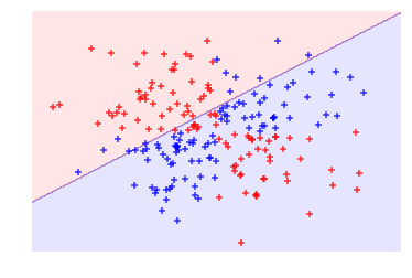
As we can see, our linear hyperplane did very poorly at dividing the two classes! Now, let’s swap out the linear kernel with a radial basis function kernel and use it to train a new model:

# Create a support vector machine with a radial basis function kernel
svc = SVC(kernel="rbf", random_state=0, gamma=1, C=1)

# Train the classifier
model = svc.fit(features, target)

And then visualize the observations and hyperplane:

# Plot observations and hyperplane
plot_decision_regions(features, target, classifier=svc)
plt.axis("off"), plt.show();

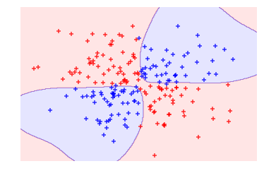
By using the radial basis function kernel we could create a decision boundary able to do a much better job of separating the two classes than the linear kernel. This is the motivation behind using kernels in support vector machines.

In scikit-learn, we can select the kernel we want to use by using the kernel parameter. Once we select a kernel, we will need to specify the appropriate kernel options such as the value of d (using the degree parameter) in polynomial kernels and γ (using the gamma parameter) in radial basis function kernels. We will also need to set the penalty parameter, C. When training the model, in most cases we should treat all of these as hyperparameters and use model selection techniques to identify the combination of their values that produces the model with the best performance.

Problem

You need to know the predicted class probabilities for an observation.

Solution

When using scikit-learn’s SVC, set probability=True, train the model, then use predict_proba to see the calibrated probabilities:

# Load libraries
from sklearn.svm import SVC
from sklearn import datasets
from sklearn.preprocessing import StandardScaler
import numpy as np

# Load data
iris = datasets.load_iris()
features = iris.data
target = iris.target

# Standardize features
scaler = StandardScaler()
features_standardized = scaler.fit_transform(features)

# Create support vector classifier object
svc = SVC(kernel="linear", probability=True, random_state=0)

# Train classifier
model = svc.fit(features_standardized, target)

# Create new observation
new_observation = [[.4, .4, .4, .4]]

# View predicted probabilities
model.predict_proba(new_observation)

array([[ 0.00588822,  0.96874828,  0.0253635 ]])

Discussion

Many of the supervised learning algorithms we have covered use probability estimates to predict classes. For example, in k-nearest neighbor, an observation’s k neighbor’s classes were treated as votes to create a probability that an observation was of that class. Then the class with the highest probability was predicted. SVC’s use of a hyperplane to create decision regions does not naturally output a probability estimate that an observation is a member of a certain class. However, we can in fact output calibrated class probabilities with a few caveats. In an SVC with two classes, Platt scaling can be used, wherein first the SVC is trained, and then a separate cross-validated logistic regression is trained to map the SVC outputs into probabilities:

where A and B are parameter vectors and f is the ith observation’s signed distance from the hyperplane. When we have more than two classes, an extension of Platt scaling is used.

In more practical terms, creating predicted probabilities has two major issues. First, because we are training a second model with cross-validation, generating predicted probabilities can significantly increase the time it takes to train our model. Second, because the predicted probabilities are created using cross-validation, they might not always match the predicted classes. That is, an observation might be predicted to be class 1, but have a predicted probability of being class 1 of less than 0.5.

In scikit-learn, the predicted probabilities must be generated when the model is being trained. We can do this by setting SVC’s probability to True. After the model is trained, we can output the estimated probabilities for each class using predict_proba.

Problem

You need to identify which observations are the support vectors of the decision hyperplane.

Solution

Train the model, then use support_vectors_:

# Load libraries
from sklearn.svm import SVC
from sklearn import datasets
from sklearn.preprocessing import StandardScaler
import numpy as np

#Load data with only two classes
iris = datasets.load_iris()
features = iris.data[:100,:]
target = iris.target[:100]

# Standardize features
scaler = StandardScaler()
features_standardized = scaler.fit_transform(features)

# Create support vector classifier object
svc = SVC(kernel="linear", random_state=0)

# Train classifier
model = svc.fit(features_standardized, target)

# View support vectors
model.support_vectors_

array([[-0.5810659 ,  0.43490123, -0.80621461, -0.50581312],
       [-1.52079513, -1.67626978, -1.08374115, -0.8607697 ],
       [-0.89430898, -1.46515268,  0.30389157,  0.38157832],
       [-0.5810659 , -1.25403558,  0.09574666,  0.55905661]])

Discussion

Support vector machines get their name from the fact that the hyperplane is being determined by a relatively small number of observations, called the support vectors. Intuitively, think of the hyperplane as being “carried” by these support vectors. These support vectors are therefore very important to our model. For example, if we remove an observation that is not a support vector from the data, the model does not change; however, if we remove a support vector, the hyperplane will not have the maximum margin.

After we have trained an SVC, scikit-learn offers us a number of options for identifying the support vector. In our solution, we used support_vectors_ to output the actual observations’ features of the four support vectors in our model. Alternatively, we can view the indices of the support vectors using support_:

model.support_

array([23, 41, 57, 98], dtype=int32)

Finally, we can use n_support_ to find the number of support vectors belonging to each class:

model.n_support_

array([2, 2], dtype=int32)

Problem

You need to train a support vector machine classifier in the presence of imbalanced classes.

Solution

Increase the penalty for misclassifying the smaller class using class_weight:

# Load libraries
from sklearn.svm import SVC
from sklearn import datasets
from sklearn.preprocessing import StandardScaler
import numpy as np

#Load data with only two classes
iris = datasets.load_iris()
features = iris.data[:100,:]
target = iris.target[:100]

# Make class highly imbalanced by removing first 40 observations
features = features[40:,:]
target = target[40:]

# Create target vector indicating if class 0, otherwise 1
target = np.where((target == 0), 0, 1)

# Standardize features
scaler = StandardScaler()
features_standardized = scaler.fit_transform(features)

# Create support vector classifier
svc = SVC(kernel="linear", class_weight="balanced", C=1.0, random_state=0)

# Train classifier
model = svc.fit(features_standardized, target)

Discussion

In support vector machines, C is a hyperparameter determining the penalty for misclassifying an observation. One method for handling imbalanced classes in support vector machines is to weight C by classes, so that:

where C is the penalty for misclassification, w_j is a weight inversely proportional to class j’s frequency, and C_j is the C value for class j. The general idea is to increase the penalty for misclassifying minority classes to prevent them from being “overwhelmed” by the majority class.

In scikit-learn, when using SVC we can set the values for C_j automatically by setting class_weight='balanced'. The balanced argument automatically weighs classes such that:

where w_j is the weight to class j, n is the number of observations, n_j is the number of observations in class j, and k is the total number of classes.