Table of Contents for
Machine Learning with Python Cookbook
 Machine Learning with Python Cookbook
Published by
O'Reilly Media, Inc., 2018
Machine Learning with Python Cookbook
Published by
O'Reilly Media, Inc., 2018
- Cover
- nav
- Machine Learning with Python Cookbook
- Machine Learning with Python Cookbook
- Preface
- Vectors, Matrices, and Arrays
- Loading Data
- Data Wrangling
- Handling Numerical Data
- Handling Categorical Data
- Handling Text
- Handling Dates and Times
- Handling Images
- Dimensionality Reduction Using Feature Extraction
- Dimensionality Reduction Using Feature Selection
- Model Evaluation
- Model Selection
- Linear Regression
- Trees and Forests
- K-Nearest Neighbors
- Logistic Regression
- Support Vector Machines
- Naive Bayes
- Clustering
- Neural Networks
- Saving and Loading Trained Models
- Index
- About the Author
- Colophon
Chapter 2. Loading Data
2.0 Introduction
The first step in any machine learning endeavor is to get the raw data into our system. The raw data might be a logfile, dataset file, or database. Furthermore, often we will want to retrieve data from multiple sources. The recipes in this chapter look at methods of loading data from a variety of sources, including CSV files and SQL databases. We also cover methods of generating simulated data with desirable properties for experimentation. Finally, while there are many ways to load data in the Python ecosystem, we will focus on using the pandas library’s extensive set of methods for loading external data, and using scikit-learn—an open source machine learning library in Python—for generating simulated data.
2.1 Loading a Sample Dataset
Solution
scikit-learn comes with a number of popular datasets for you to use:
# Load scikit-learn's datasetsfromsklearnimportdatasets# Load digits datasetdigits=datasets.load_digits()# Create features matrixfeatures=digits.data# Create target vectortarget=digits.target# View first observationfeatures[0]
array([  0.,   0.,   5.,  13.,   9.,   1.,   0.,   0.,   0.,   0.,  13.,
        15.,  10.,  15.,   5.,   0.,   0.,   3.,  15.,   2.,   0.,  11.,
         8.,   0.,   0.,   4.,  12.,   0.,   0.,   8.,   8.,   0.,   0.,
         5.,   8.,   0.,   0.,   9.,   8.,   0.,   0.,   4.,  11.,   0.,
         1.,  12.,   7.,   0.,   0.,   2.,  14.,   5.,  10.,  12.,   0.,
         0.,   0.,   0.,   6.,  13.,  10.,   0.,   0.,   0.])
Discussion
Often we do not want to go through the work of loading, transforming, and cleaning a real-world dataset before we can explore some machine learning algorithm or method. Luckily, scikit-learn comes with some common datasets we can quickly load. These datasets are often called “toy” datasets because they are far smaller and cleaner than a dataset we would see in the real world. Some popular sample datasets in scikit-learn are:
load_boston-
Contains 503 observations on Boston housing prices. It is a good dataset for exploring regression algorithms.
load_iris-
Contains 150 observations on the measurements of Iris flowers. It is a good dataset for exploring classification algorithms.
load_digits-
Contains 1,797 observations from images of handwritten digits. It is a good dataset for teaching image classification.
2.2 Creating a Simulated Dataset
Problem
You need to generate a dataset of simulated data.
Solution
scikit-learn offers many methods for creating simulated data. Of those, three methods are particularly useful.
When we want a dataset designed to be used with linear regression,
make_regression is a good choice:
# Load libraryfromsklearn.datasetsimportmake_regression# Generate features matrix, target vector, and the true coefficientsfeatures,target,coefficients=make_regression(n_samples=100,n_features=3,n_informative=3,n_targets=1,noise=0.0,coef=True,random_state=1)# View feature matrix and target vector('Feature Matrix\n',features[:3])('Target Vector\n',target[:3])
Feature Matrix
 [[ 1.29322588 -0.61736206 -0.11044703]
 [-2.793085    0.36633201  1.93752881]
 [ 0.80186103 -0.18656977  0.0465673 ]]
Target Vector
 [-10.37865986  25.5124503   19.67705609]
If we are interested in creating a simulated dataset for classification,
we can use make_classification:
# Load libraryfromsklearn.datasetsimportmake_classification# Generate features matrix and target vectorfeatures,target=make_classification(n_samples=100,n_features=3,n_informative=3,n_redundant=0,n_classes=2,weights=[.25,.75],random_state=1)# View feature matrix and target vector('Feature Matrix\n',features[:3])('Target Vector\n',target[:3])
Feature Matrix
 [[ 1.06354768 -1.42632219  1.02163151]
 [ 0.23156977  1.49535261  0.33251578]
 [ 0.15972951  0.83533515 -0.40869554]]
Target Vector
 [1 0 0]
Finally, if we want a dataset designed to work well with clustering
techniques, scikit-learn offers make_blobs:
# Load libraryfromsklearn.datasetsimportmake_blobs# Generate feature matrix and target vectorfeatures,target=make_blobs(n_samples=100,n_features=2,centers=3,cluster_std=0.5,shuffle=True,random_state=1)# View feature matrix and target vector('Feature Matrix\n',features[:3])('Target Vector\n',target[:3])
Feature Matrix
 [[ -1.22685609   3.25572052]
 [ -9.57463218  -4.38310652]
 [-10.71976941  -4.20558148]]
Target Vector
 [0 1 1]
Discussion
As might be apparent from the solutions, make_regression returns a feature matrix of float values and a target vector of float values,
while make_classification and make_blobs return a feature matrix of
float values and a target vector of integers representing membership in
a class.
scikit-learn’s simulated datasets offer extensive options to control the type of data generated. scikit-learn’s documentation contains a full description of all the parameters, but a few are worth noting.
In make_regression and make_classification, n_informative
determines the number of features that are used to generate the target
vector. If n_informative is less than the total number of features
(n_features), the resulting dataset will have redundant features
that can be identified through feature selection techniques.
In addition, make_classification contains a weights parameter that allows us to simulate datasets with imbalanced classes. For example,
weights = [.25, .75] would return a dataset with 25% of observations belonging to one class and 75% of observations belonging to a second
class.
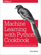
For make_blobs, the centers parameter determines the number of
clusters generated. Using the matplotlib visualization library, we can
visualize the clusters generated by make_blobs:
# Load libraryimportmatplotlib.pyplotasplt# View scatterplotplt.scatter(features[:,0],features[:,1],c=target)plt.show()
2.3 Loading a CSV File
Solution
Use the pandas library’s read_csv to load a local or hosted CSV file:
# Load libraryimportpandasaspd# Create URLurl='https://tinyurl.com/simulated_data'# Load datasetdataframe=pd.read_csv(url)# View first two rowsdataframe.head(2)
| integer | datetime | category | |
|---|---|---|---|
| 0 | 5 | 2015-01-01 00:00:00 | 0 |
| 1 | 5 | 2015-01-01 00:00:01 | 0 |
Discussion
There are two things to note about loading CSV files. First, it is often
useful to take a quick look at the contents of the file before loading.
It can be very helpful to see how a dataset is structured beforehand and
what parameters we need to set to load in the file. Second, read_csv
has over 30 parameters and therefore the documentation can be daunting.
Fortunately, those parameters are mostly there to allow it to handle a
wide variety of CSV formats. For example, CSV files get their names from
the fact that the values are literally separated by commas (e.g., one row might be 2,"2015-01-01 00:00:00",0); however, it is common for “CSV” files to use other characters as separators, like tabs. pandas’ sep parameter allows us to define the delimiter used in the file. Although it is not always the case, a common formatting issue with CSV files is that the first line of the file is used to define column headers (e.g., integer, datetime, category in our solution). The header parameter allows us to specify if or where a header row exists. If a header row does not exist, we set header=None.
2.4 Loading an Excel File
Solution
Use the pandas library’s read_excel to load an Excel spreadsheet:
# Load libraryimportpandasaspd# Create URLurl='https://tinyurl.com/simulated_excel'# Load datadataframe=pd.read_excel(url,sheetname=0,header=1)# View the first two rowsdataframe.head(2)
| 5 | 2015-01-01 00:00:00 | 0 | |
|---|---|---|---|
| 0 | 5 | 2015-01-01 00:00:01 | 0 |
| 1 | 9 | 2015-01-01 00:00:02 | 0 |
Discussion
This solution is similar to our solution for reading CSV files. The main
difference is the additional parameter, sheetname, that specifies which sheet in the Excel file we wish to load. sheetname can accept both strings containing the name of the sheet and integers pointing to sheet positions (zero-indexed). If we need to load multiple sheets, include them as a list. For example, sheetname=[0,1,2, "Monthly Sales"] will return a dictionary of pandas DataFrames containing the first, second, and third sheets and the sheet named Monthly Sales.
2.5 Loading a JSON File
Solution
The pandas library provides read_json to convert a JSON file into a
pandas object:
# Load libraryimportpandasaspd# Create URLurl='https://tinyurl.com/simulated_json'# Load datadataframe=pd.read_json(url,orient='columns')# View the first two rowsdataframe.head(2)
category
datetime
integer
0
0
2015-01-01 00:00:00
5
1
0
2015-01-01 00:00:01
5
Discussion
Importing JSON files into pandas is similar to the last few recipes we
have seen. The key difference is the orient parameter, which indicates
to pandas how the JSON file is structured. However, it might take some
experimenting to figure out which argument (split, records, index,
columns, and values) is the right one. Another helpful tool pandas
offers is json_normalize, which can help convert semistructured JSON data into a pandas DataFrame.
See Also
2.6 Querying a SQL Database
Solution
pandas’ read_sql_query allows us to make a SQL query to a database and
load it:
# Load librariesimportpandasaspdfromsqlalchemyimportcreate_engine# Create a connection to the databasedatabase_connection=create_engine('sqlite:///sample.db')# Load datadataframe=pd.read_sql_query('SELECT * FROM data',database_connection)# View first two rowsdataframe.head(2)
| first_name | last_name | age | preTestScore | postTestScore | |
|---|---|---|---|---|---|
| 0 | Jason | Miller | 42 | 4 | 25 |
| 1 | Molly | Jacobson | 52 | 24 | 94 |
Discussion
Out of all of the recipes presented in this chapter, this recipe is
probably the one we will use most in the real world. SQL is the lingua
franca for pulling data from databases. In this recipe we first use
create_engine to define a connection to a SQL database engine called SQLite. Next we use pandas’ read_sql_query to query that database
using SQL and put the results in a DataFrame.
SQL is a language in its own right and, while beyond the scope of this
book, it is certainly worth knowing for anyone wanting to learn machine
learning. Our SQL query, SELECT * FROM data, asks the database to give
us all columns (*) from the table called data.