Table of Contents for
Machine Learning and Security
 Machine Learning and Security
Published by
O'Reilly Media, Inc., 2018
Machine Learning and Security
Published by
O'Reilly Media, Inc., 2018
- nav
- Cover
- Praise for Machine Learning and Security
- Machine Learning and Security
- Machine Learning and Security
- Preface
- 1. Why Machine Learning and Security?
- 2. Classifying and Clustering
- 3. Anomaly Detection
- 4. Malware Analysis
- 5. Network Traffic Analysis
- 6. Protecting the Consumer Web
- 7. Production Systems
- 8. Adversarial Machine Learning
- A. Supplemental Material for Chapter 2
- B. Integrating Open Source Intelligence
- Index
- About the Authors
- Colophon
Chapter 8. Adversarial Machine Learning
As machine learning begins to be ubiquitously deployed in critical systems, its reliability naturally comes under scrutiny. Although it is important not to be alarmist, the threat that adversarial agents pose to machine learning systems is real. Much like how a hacker might take advantage of a firewall vulnerability to gain access to a web server, a machine learning system can itself be targeted to serve the goals of an attacker. Hence, before putting such solutions in the line of fire, it is crucial to consider their weaknesses and understand how malleable they are under stress.
Adversarial machine learning is the study of machine learning vulnerabilities in adversarial environments. Security and machine learning researchers have published research on practical attacks against machine learning antivirus engines,1 spam filters,2 network intrusion detectors, image classifiers,3 sentiment analyzers,4,5 and more. This has been an increasingly active area of research in recent times, even though such attacks have rarely been observed in the wild. When information security, national sovereignties, and human lives are at stake, machine learning system designers have a responsibility to preempt attacks and build safeguards into these systems.
Vulnerabilities in machine learning systems can arise from flawed system design, fundamental algorithmic limitations, or a combination of both. In this chapter, we examine some vulnerabilities in and attacks on machine learning algorithms. We then use the knowledge gained to motivate system designs that are more resilient to attacks.
Terminology
Early research in adversarial machine learning defined a taxonomy for qualitatively analyzing attacks on machine learning systems based on three dimensions of properties:6
- Influence
-
Causative attacks refer to attempts by an adversarial actor to affect the training process by tampering with the training data or training phase parameters. Because it is difficult for an adversary to manipulate an offline curated training set, this type of attack is predominately relevant to online learners. Online learners automatically adapt to changing data distributions by directly exploiting user interactions or feedback on predictions to update the trained model. By sacrificing stationarity for adaptability, such learning systems continuously evolve by incrementally training statistical models with freshly observed data. Typical use cases of online learning include an image classification service that learns from user corrections and reinforcement, or malicious traffic detection on websites that frequently experience viral traffic spikes.
Exploratory attacks are purely based on post–training phase interactions with machine learning systems. In this mode of attack, actors do not have any influence over the trained data manifold, but instead find and exploit adversarial space to cause models to make mistakes that they were not designed to make. A naive example of an exploratory attack is to engage in brute-force fuzzing of a machine learning classifier’s input space to find samples that are wrongly classified.
- Specificity
-
Targeted attacks refer to attempts to cause a directed and intentional shift of a model’s predictions to an alternate, focused outcome. For instance, a targeted attack of a malware family classifier could cause samples belonging to malware family A to be reliably misclassified as malware family B.
Indiscriminate attacks are highly unspecific attacks by adversaries who want models to make wrong decisions but don’t necessarily care what the eventual outcome of the system is. An indiscriminate attack on the malware family classifier just mentioned would cause samples belonging to malware family A to be misclassified as anything but family A.
- Security violation
-
Integrity attacks on machine learning systems affect only the ability of security detectors to find attacks; that is, they reduce the true positive rate (i.e., recall). A successful launch of such an attack on a machine learning web application firewall would mean that an adversary can successfully execute attacks that the firewall was specifically designed to detect.
Availability attacks, which are usually the result of indiscriminate attacks, degrade the usability of a system by reducing the true positive rate and increasing the false positive rate. When systems fail in this manner, it becomes difficult to reliably act on the results produced and hence the attack is viewed as a reduction in system availability. This type of attack is relevant only to causative attacks because it typically involves tampering with an (online) learning agent’s decision functions.
The Importance of Adversarial ML
Machine learning is quickly becoming a compulsory tool in any security practitioner’s repertoire, but three out of four researchers still feel that today’s artificial intelligence–driven security solutions are flawed.7 A large part of the lack of confidence in security machine learning solutions stems from the ease with which adversaries can bypass such solutions. The interesting conundrum is that many security professionals also predict that security solutions of the future will be driven by AI and machine learning. The need to close the gap between the reality of today and the expectations for tomorrow explains why adversarial machine learning is important to consider for security contexts.
Adversarial machine learning is difficult because most machine learning solutions behave as black boxes. The lack of transparency into what goes on inside detectors and classifiers makes it difficult for users and practitioners to make sense of model predictions. Furthermore, the lack of explainability of decisions made by these systems means that users cannot easily detect when a system has been influenced by a malicious actor. As long as humans cannot be assured of robustness of machine learning systems, there will be resistance to their adoption and acceptance as a main driver in security solutions.
Security Vulnerabilities in Machine Learning Algorithms
Security systems are natural targets for malicious tampering because there are often clear gains for attackers who successfully circumvent them. Systems powered by machine learning contain a fresh new attack surface that adversaries can exploit when they are furnished with background knowledge in this space. Hacking system environments by exploiting design or implementation flaws is nothing new, but fooling statistical models is another matter altogether. To understand the vulnerabilities of machine learning algorithms, let’s consider the how the environment in which these techniques are applied affects their performance. As an analogy, consider a swimmer who learns and practices swimming in swimming pools their entire life. It is likely that they will be a strong swimmer in pools, but if they are suddenly thrown into the open ocean, they might not be equipped with the ability to deal with strong currents and hostile conditions and are likely to struggle.
Machine learning techniques are usually developed under the assumptions of data stationarity, feature independence, and weak stochasticity. Training and testing datasets are assumed to be drawn from populations whose distributions don’t change over time, and selected features are assumed to be independently and identically distributed. Machine learning algorithms are not typically designed to be effective in adversarial environments where these assumptions are shattered. Attempting to fit a descriptive and lasting model to detect adaptive adversaries that have incentive to avoid correct classification is a difficult task. Adversaries will attempt to break any assumptions that practitioners make as long as that is the path of least resistance into a system.
A large class of machine learning vulnerabilities arise from the fundamental problem of imperfect learning. A machine learning algorithm attempts to fit a hypothesis function that maps points drawn from a certain data distribution space into different categories or onto a numerical spectrum. As a simple thought experiment, suppose that you want to train a statistical learning agent to recognize cross-site scripting (XSS) attacks8 on web applications. The ideal result is an agent that is able to detect every possible permutation of XSS input with perfect accuracy and no false positives. In reality, we will never be able to produce systems with perfect efficacy that solve meaningfully complex problems because the learner cannot be provided with perfect information. We are not able to provide the learner with a dataset drawn from the entire distribution of all possible XSS input. Hence, there exists a segment of the distribution that we intend for the learner to capture but that we have not actually provided it sufficient information to learn about. Modeling error is another phenomenon that contributes to the adversarial space of a statistical learner. Statistical learning forms abstract models that describe real data, and modeling error arises due to natural imperfections that occur in these formed models.
Even “perfect learners” can display vulnerabilities because the Bayes error rate9 might be nonzero. The Bayes error rate is the lower bound on the possible error for a given combination of a statistical classifier and the set of features used. This error rate is useful for assessing the quality of a feature set, as well as measuring the effectiveness of a classifier. The Bayes error rate represents a theoretical limit for a classifier’s performance, which means that even when we provide a classifier with a complete representation of the data, eliminating any sources of imperfect learning, there still exists a finite set of adversarial samples that can cause misclassifications.
Figure 8-1 illustrates the theoretical data population we want to develop a statistical learning model for, and its relationships with the training and test data distribution spaces. (Note that we are referring not to the actual datasets, but to the population from which these datasets are drawn—there should be no intersection between the training and test datasets.)
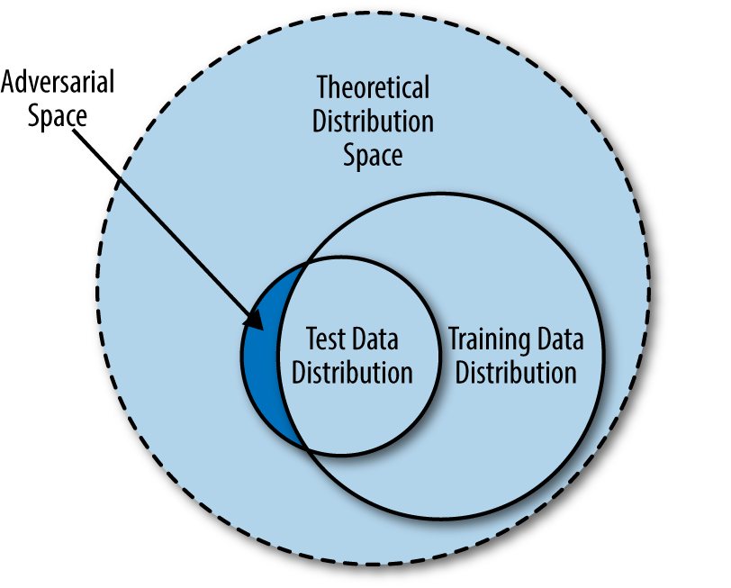
Figure 8-1. Adversarial space as a result of imperfect representation in training data
Essentially, the training data we provide a machine learning algorithm is drawn from an incomplete segment of the theoretical distribution space. When the time comes for evaluation of the model in the lab or in the wild, the test set (drawn from the test data distribution) could contain a segment of data whose properties are not captured in the training data distribution; we refer to this segment as adversarial space. Attackers can exploit pockets of adversarial space between the data manifold fitted by a statistical learning agent and the theoretical distribution space to fool machine learning algorithms. Machine learning practitioners and system designers expect the training and test data to be drawn from the same distribution space, and further assume that all characteristics of the theoretical distribution be covered by the trained model. These “blind spots” in machine learning algorithms arise because of the discrepancy between expectation and reality.
More catastrophically, when attackers are able to influence the training phase, they can challenge the data stationarity assumptions of machine learning processes. Systems that perform online learning (i.e., that learn from real-time user feedback) are not uncommon because of adaptability requirements and the benefits that self-adjusting statistical systems bring. However, online learning introduces a new class of model poisoning vulnerabilities that we must consider.
Statistical learning models derive intelligence from data fed into them, and vulnerabilities of such systems naturally stem from inadequacies in the data. As practitioners, it is important to ensure that the training data is as faithful a representation of the actual distribution as possible. At the same time, we need to continually engage in proactive security defense and be aware of different attack vectors so that we can design algorithms and systems that are more resilient to attacks.
Attack Transferability
The phenomenon of attack transferability was discovered by researchers who found that adversarial samples (drawn from adversarial space) that are specifically designed to cause a misclassification in one model are also likely to cause misclassifications in other independently trained models10,11—even when the two models are backed by distinctly different algorithms or infrastructures.12 It is far from obvious why this should be the case, given that, for example, the function that a support vector machine fits to a training data distribution presumably bears little resemblance to the function fit by a deep neural network. Put in a different way, the adversarial spaces in the data manifold of trained machine learning model A have been found to overlap significantly with the adversarial spaces of an arbitrary model B.
Transferability of adversarial attacks has important consequences for practical attacks on machine learning because model parameters are not commonly exposed to users interacting with a system. Researchers have developed practical adversarial evasion attacks on so-called black-box models; i.e., classifiers for which almost no information about the machine learning technique or model used is known.13 With access only to test samples and results from the black-box classifier, we can generate a labeled training dataset with which we can train a local substitute model. We then can analyze this local substitute model offline to search for samples that belong to adversarial space. Subsequently, attack transferability allows us to use these adversarial samples to fool the remote black-box model.
Attack transferability is an active area of research,14 and this work will continue to influence the field of adversarial machine learning in the foreseeable future.
Attack Technique: Model Poisoning
Model poisoning attacks, also known as red herring17 attacks, are realistically observed only in online learning systems. Online learning systems sacrifice stationarity for adaptability by dynamically retraining machine learning models with fresh user interactions or feedback. Anomaly detection systems use online learning to automatically adjust model parameters over time as they detect changes in normal traffic. In this way, laborious human intervention to continually tune models and adjust thresholds can be avoided. Nevertheless, online learners come with a set of risks in adversarial environments. Especially in systems that are not well designed for resilience to attacker manipulation, it can be trivial for an adversary to confuse machine learning algorithms by introducing synthetic traffic.
By definition, poisoning attacks are causative in nature and can vary arbitrarily in specificity and type of security violation. Consider a natural language translation service with a naively implemented online user feedback loop that takes in user corrections to continually retrain the machine learning translation engine. Without any form of input filtering, an indiscriminate attack on the system could be as simple as providing nonsensical garbage feedback, as in Figure 8-2.18 A more targeted attack could be made to the system by selectively and repeatedly causing the system to translate the word “love” in English to “déteste” in French, as shown in Figure 8-3.
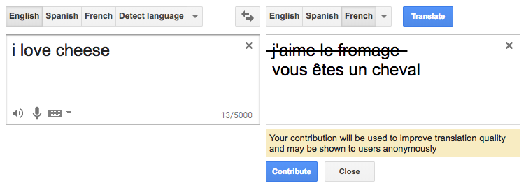
Figure 8-2. Indiscriminate poisoning of a language translation system
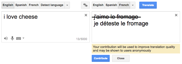
Figure 8-3. Targeted poisoning of a language translation system
It is easy to understand how a model can be negatively affected by such input. The worldview of a statistical learning agent is shaped entirely by the training data it receives and any positive or negative reinforcement of its learned hypotheses. When a toddler is learning the names of fruits through examples in a picture book, the learning process can similarly be poisoned if the example fruits in the book are incorrectly named.
In poisoning attacks, attackers are assumed to have control over a portion of the training data used by the learning algorithm. The larger the proportion of training data that attackers have control over, the more influence they have over the learning objectives and decision boundaries of the machine learning system.19 An attacker who has control over 50% of the training set can influence the model to a greater extent than an attacker who has control over only 5%. This implies that more popular services that see a larger volume of legitimate traffic are more difficult to poison because attackers need to inject a lot more chaff20 to have any meaningful impact on the learning outcome.
Of course, system owners can easily detect when an online learner receives a high volume of garbage training data out of the blue. Simple rules can flag instances of sudden spikes in suspicious or abnormal behavior that can indicate malicious tampering. After you detect it, filtering out this traffic is trivial. That said, if attackers throttle their attack traffic, they can be a lot more difficult to detect. So-called boiling frog attacks spread out the injection of adversarial training examples over an extended period of time so as not to trigger any tripwires. Boiling frog attacks can be made more effective and less suspicious by introducing chaff traffic in stages that match the gradual shifting of the classifier’s decision boundary.
Poisoning attacks executed gradually over a long period of time can be made to look like organic drift in the data distributions. For instance, an online learning anomaly detector that has a decision boundary initially fitted to block at 10 requests per minute (per IP address) would block requests from IPs that make 20 requests per minute. The system would be unlikely to be configured to learn from this traffic because the detector would classify this as an anomaly with high confidence. However, sticking closer to the decision boundary can cause these systems to “second-guess” the initially fitted hypothesis functions. An attacker that starts by sending 11 requests per minute for one week can have a higher chance of moving the decision boundary from 10 to 11. Repeating this process with the new boundary can help achieve the original goal of significantly altering the decision boundary without raising any alarms. To system administrators, there can be a variety of legitimate reasons for this movement: increased popularity of a website, increased user retention leading to longer interactions, introduction of new user flows, and so on.
Poisoning attacks have been studied and demonstrated on a variety of different machine learning techniques and practical systems: SVMs;21 centroid and generic anomaly detection algorithms;22,23 logistic, linear, and ridge regression;24 spam filters;25 malware classifiers;26 feature selection processes;27 PCA;28 and deep learning algorithms.29
Example: Binary Classifier Poisoning Attack
To concretely illustrate poisoning attacks, let’s demonstrate exactly how the decision boundary of a simple machine learning classifier can be manipulated by an attacker with unbounded query access to system predictions.30 We begin by creating a random synthetic dataset using the sklearn.datasets.make_classification() utility:
fromsklearn.datasetsimportmake_classificationX,y=make_classification(n_samples=200,n_features=2,n_informative=2,n_redundant=0,weights=[.5,.5],random_state=17)
This code is a simple two-feature dataset with 200 samples, out of which we will use the first 100 samples to train the classifier and the next 100 to visually demonstrate that the classifier is appropriately fitted.
For our example, we fit a multilayer perceptron (MLP) classifier to this dataset.31 MLPs are a class of simple feed-forward neural networks that can create nonlinear decision boundaries. We import the sklearn.neural_network.MLPClassifier class and fit the model to our dataset:
fromsklearn.neural_networkimportMLPClassifierclf=MLPClassifier(max_iter=600,random_state=123).fit(X[:100],y[:100])
To inspect what’s going on under the hood, let’s generate a visualization of the classifier’s decision function. We create a two-dimensional mesh grid of points in our input space (X and y values between −3 and 3 with intervals of .01 between each adjacent point) and then extract prediction probabilities for each of the points in this mesh:
importnumpyasnpxx,yy=np.mgrid[-3:3:.01,−3:3:.01]grid=np.c_[xx.ravel(),yy.ravel()]probs=clf.predict_proba(grid)[:,1].reshape(xx.shape)
Then we generate a contour plot from this information and overlay the test set on the plot, displaying X1 on the vertical axis and X0 on the horizontal axis:
importmatplotlib.pyplotaspltf,ax=plt.subplots(figsize=(12,9))# Plot the contour backgroundcontour=ax.contourf(xx,yy,probs,25,cmap="RdBu",vmin=0,vmax=1)ax_c=f.colorbar(contour)ax_c.set_label("$P(y = 1)$")ax_c.set_ticks([0,.25,.5,.75,1])# Plot the test set (latter half of X and y)ax.scatter(X[100:,0],X[100:,1],c=y[100:],s=50,cmap="RdBu",vmin=-.2,vmax=1.2,edgecolor="white",linewidth=1)ax.set(aspect="equal",xlim=(-3,3),ylim=(-3,3))
Figure 8-4 shows the result.
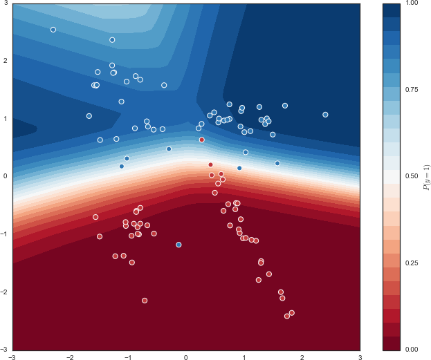
Figure 8-4. Decision function contour plot of MLP classifier fitted to our dataset
Figure 8-4 shows that the MLP’s decision function seems to fit quite well to the test set. We use the confidence threshold of 0.5 as our decision boundary. That is, if the classifier predicts that P(y = 1) > 0.5, the prediction is y = 1; otherwise, the prediction is y = 0. We define a utility function plot_decision_boundary() for plotting this decision boundary along with the same test set:32
plot_decision_boundary(X,y,probs)
Figure 8-5 shows the result.
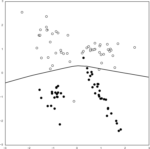
Figure 8-5. Decision boundary of MLP classifier fitted to our dataset
We then generate five carefully selected chaff points, amounting to just 5% of the training dataset. We assign the label y = 1 to these points because that is what the classifier would predict (given the current decision function):
num_chaff=5chaff_X=np.array([np.linspace(-2,−1,num_chaff),np.linspace(0.1,0.1,num_chaff)]).Tchaff_y=np.ones(num_chaff)
Figure 8-6 illustrates the chaff points (depicted by the star markers), which mostly lie within the y = 1 space (y = 1 is depicted by empty circle markers, and y = 0 is depicted by the filled circle markers).
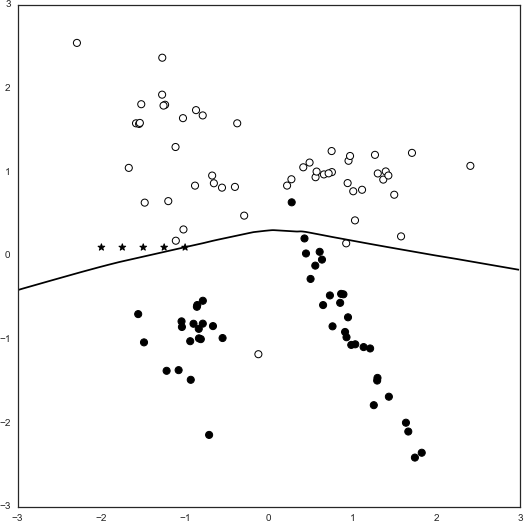
Figure 8-6. Chaff points depicted in relation to the test set
To mimic online learners that use newly received data points to dynamically and incrementally train the machine learning model, we are going to use scikit-learn’s partial_fit() API for incremental learning that some estimators (including MLPClassifier) implement. We incrementally train our existing classifier by partial-fitting the model to the five new chaff points (attack traffic) that we generated:
clf.partial_fit(chaff_X,chaff_y)
The classifier is now updated with this new malicious information. Now, let’s see how the decision boundary has shifted (see Figure 8-7):
probs_poisoned=clf.predict_proba(grid)[:,1].reshape(xx.shape)plot_decision_boundary(X,y,probs,chaff_X,chaff_y,probs_poisoned)
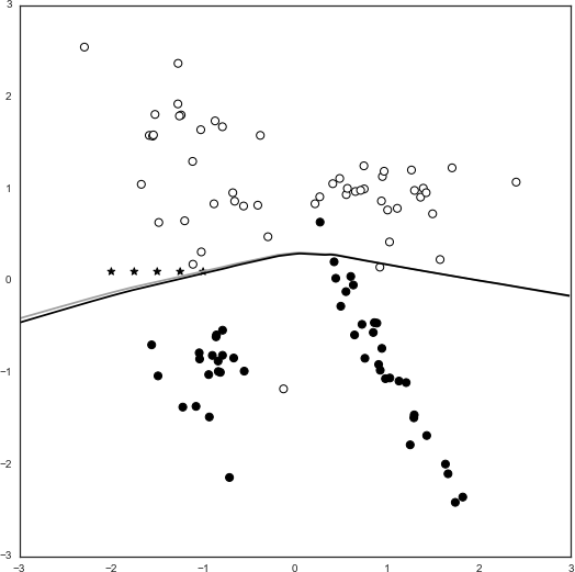
Figure 8-7. Shifted decision boundary after 1x partial fitting of five chaff points
The new decision boundary is the darker of the two curves. Notice that the decision boundary has shifted slightly downward, creating a miniscule gap between the two curves. Any points that lie within this gap would previously have been classified as y = 0, but now would be classified as y = 1. This means that the attacker has been successful in causing a targeted misclassification of samples. Repeating the partial_fit() step iteratively (using the same five chaff points) allows us to observe how much the decision function shifts as the percentage of chaff traffic increases, as demonstrated in Figure 8-8.
A larger-magnitude shift of the decision boundary represents a larger input space of misclassified points, which implies a more serious degradation of model performance.
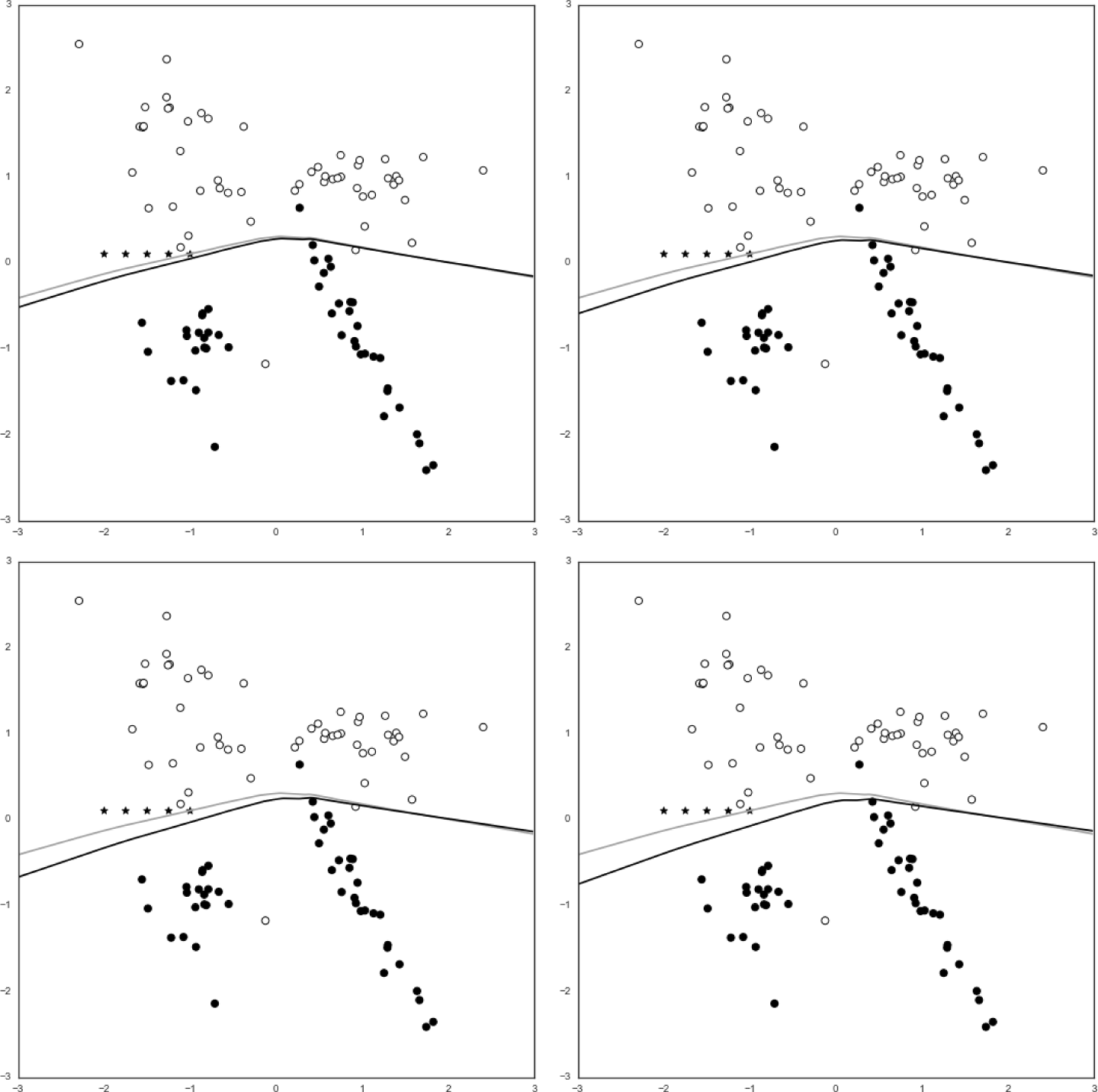
Figure 8-8. Shifted decision boundaries after 2x, 3x, 4x, and 5x partial fitting of five chaff points (10%, 15%, 20%, 25% attack traffic from upper left to lower right, respectively)
Attacker Knowledge
As you might notice from Figure 8-8, knowledge of the underlying model’s decision function is an important factor in poisoning attacks. How does the attacker know how to select chaff in a way that will cause an effective shift of the decision boundary?
The basic level of access that we assume that any attacker has is the ability to launch an unlimited number of queries to the system and obtain a prediction result. That said, the fewer queries made to a system, the less likely an attacker is to trigger tripwires and cause suspicion. An attacker who has access not only to the prediction result but also to the prediction probabilities is in a much more powerful position because they can then derive decision function gradients (such as those shown in Figure 8-4) that allow for useful optimizations, especially when selecting chaff points on complex decision function surfaces; for example, when the decision function has multiple local minima or maxima.
However, even an attacker without access to the prediction probabilities has access to categorical classification results, which then allows them to infer the decision boundaries of a model by making queries to points around the boundary line (as shown in Figures 8-5 through 8-8). This information is enough for an attacker to select chaff traffic that does not arouse suspicion yet can mislead an online learner.
One scenario in which determining chaff placement requires a bit more reverse engineering of the machine learning system is when the input data is transformed before being fed into a classifier. For instance, if PCA dimensionality reduction is applied to the data, how does an attacker know which dimensions of the input to manipulate? Similarly, if the input goes through some other unknown nonlinear transformation before being fed into a classifier, it is a lot less clear how an attacker should map changes in the raw input to points on the decision surface. As another example, some types of user input cannot be easily modified by a user interacting with the system, such as when classifier input depends on system state or properties that users have no influence over. Finally, determining how much chaff is necessary to cause a meaningful shift of the decision boundary can also be challenging.
The aforementioned challenges can mostly be overcome with enough access to the system, allowing the attacker to extract as much information from a learner as possible. As defenders, the goal is to make it difficult for attackers to make simple inferences about the system that allow them to engage in attacks on the learner without sacrificing the system’s efficacy.
Defense Against Poisoning Attacks
There are some design choices that a machine learning system architect can make that will make it more difficult for even motivated adversaries to poison models. Does the system really need real-time, minute-by-minute online learning capabilities, or can similar value be obtained from a daily scheduled incremental training using the previous day’s data? There are significant benefits to designing online learning systems that behave similarly to an offline batch update system:
-
Having longer periods between retraining gives systems a chance to inspect the data being fed into the model.
-
Analyzing a longer period of data gives systems a better chance of detecting boiling frog attacks, where chaff is injected gradually over longer periods of time. Aggregating a week’s worth of data, as opposed to the past five minutes of data, allows you to detect chaff being injected at a low rate.
-
Attackers thrive on short feedback loops. A detectable shift in the decision boundary as a result of their attack traffic gives them quick positive reinforcement and allows them to continue iterating on their method. Having a week-long update cycle means that attackers will not know if their attack attempt will have the positive outcome they are looking for until the following week.
If you have a mechanism for inspecting incremental training data before feeding it into a partial learning algorithm, there are several ways you can detect poisoning attack attempts:
-
Identifying abnormal pockets of traffic that originate from a single IP address or autonomous system (ASN), or have unusual common characteristics; for example, many requests coming in with an abnormal user agent string. You can remove such traffic from the automatic incremental learning mechanism and have an analyst inspect the traffic for signs of attacks.
-
Maintaining a calibration set of handcrafted “normal traffic” test data that you run against the model after each period of retraining. If the classification results differ dramatically between previous cycles and the current cycle, there might be tampering involved.
-
Defining a threshold around the decision boundary and continuously measuring what percentage of test data points observed fall in that space. For example, suppose that you have a simple linear decision boundary at P(y = 1) = 0.5. If you define the decision boundary threshold region to be 0.4 < P(y = 1) < 0.6, you can count the percentage of test data points observed daily that fall within this region of prediction confidence. If, say, 30% of points fall in this region on average, and you suddenly have 80% of points falling into this region over the past week, this anomaly might signify a poisoning attack—attackers will try to stick as close to the decision boundary as possible to maximize the chances of shifting the boundary without raising alarms.
Because of the large variety of model poisoning attacks that can be launched on a machine learning system, there is no hard-and-fast rule for how to definitively secure a system on this front. This field is an active area of research, and there continue to be algorithmic developments in statistical learning techniques that are less susceptible to poisoning attacks. Robust statistics is frequently cited as a potential solution to make algorithms more resilient to malicious tampering.33,34,35,36,37
Attack Technique: Evasion Attack
Exploiting adversarial space (illustrated in Figure 8-1) to find adversarial examples that cause a misclassification in a machine learning classifier is called an evasion attack. Popular media has compared this phenomenon to humans being fooled by optical illusions, mainly because early research in this area demonstrated the concept on deep neural net image classifiers.38 For example, Figure 8-9 illustrates how small alterations made to individual pixel intensities can cause a high-performance MNIST digit classifier to misclassify the 0 as a 6.

Figure 8-9. Comparison of the unaltered MNIST handwritten digit of a 0 (left) with the adversarially perturbed version (right)
Evasion attacks are worthy of concern because they are more generally applicable than poisoning attacks. For one, these attacks can affect any classifier, even if the user has no influence over the training phase. In combination with the phenomenon of adversarial transferability and local substitute model training, the exploratory nature of this technique means that motivated attackers can launch highly targeted attacks on the integrity of a large class of machine learning systems. Evasion attacks with adversarial examples have been shown to have a significant impact on both traditional machine learning models (logistic regression, SVMs, nearest neighbor, decision trees, etc.) and deep learning models.
Researchers have also shown that image misclassifications can have significant real-world consequences.39 In particular, the development of autonomous vehicles has led researchers to find adversarial examples that are robust to arbitrary noise and transformations,40 and it has been shown that very small perturbations made to street signs can cause targeted misclassifications of the images in self-driving cars.41
Of course, this type of attack is not limited to image classification systems. Researchers have demonstrated a similar attack to successfully evade malware classifiers,42 which has direct consequences on the security industry’s confidence in machine learning as a driver of threat detection engines. Adversarial perturbations are convenient to apply to image samples because altering a few pixels of an image typically does not have obvious visual effects. Applying the same concept to executable binaries, on the other hand, requires some hacking and experimentation to ensure that the bits perturbed (or program instructions, lines of code, etc.) will not cause the resulting binary to be corrupted or lose its original malicious behavior, which would defeat the entire purpose of evasion.
Example: Binary Classifier Evasion Attack
Let’s demonstrate the principles of evasion attacks by attempting to find an adversarial example using a rudimentary gradient ascent algorithm. Assuming a perfect-knowledge attacker with full access to the trained machine learning model:
-
We begin with an arbitrarily chosen sample and have the model generate prediction probabilities for it.
-
We dissect the model to find features that are the most strongly weighted in the direction that we want the misclassification to occur; that is, we find a feature J that causes the classifier to be less confident in its original prediction.
-
We iteratively increase the magnitude of the feature until the prediction probability crosses the confidence threshold (typically 0.5).
The pretrained machine learning model that we will be working on is a simple web application firewall (WAF).43 This WAF is a dedicated XSS classifier. Given a string, the WAF will predict whether the string is an instance of XSS. Give it a spin!
Even though real-world attackers will have less than perfect knowledge, assuming a perfect-knowledge attacker enables us to perform a worst-case evaluation of model vulnerabilities and demonstrate some upper bounds on these attacks. In this case, we assume the attacker has access to a serialized scikit-learn Pipeline object and can inspect each stage in the model pipeline.
First, we load the trained model and see what steps the pipeline contains using the Python built-in vars() function:44
importpicklep=pickle.load(open('waf/trained_waf_model'))vars(p)>{'steps':[('vectorizer',TfidfVectorizer(analyzer='char',binary=False,decode_error=u'strict',dtype=<type'numpy.int64'>,encoding=u'utf-8',input=u'content',lowercase=True,max_df=1.0,max_features=None,min_df=0.0,ngram_range=(1,3),norm=u'l2',preprocessor=None,smooth_idf=True,stop_words=None,strip_accents=None,sublinear_tf=True,token_pattern=u'(?u)\\b\\w\\w+\\b',tokenizer=None,use_idf=True,vocabulary=None)),('classifier',LogisticRegression(C=1.0,class_weight='balanced',dual=False,fit_intercept=True,intercept_scaling=1,max_iter=100,multi_class='ovr',n_jobs=1,penalty='l2',random_state=None,solver='liblinear',tol=0.0001,verbose=0,warm_start=False))]}
We see that the Pipeline object contains just two steps: a TfidfVectorizer followed by a LogisticRegression classifier. A successful adversarial example, in this case, should cause a false negative; specifically, it should be a string that is a valid XSS payload but is classified as a benign string by the classifier.
Given our previous knowledge of text vectorizers, we know that we now need to find the particular string tokens that can help influence the classifier the most. We can inspect the vectorizer’s token vocabulary by inspecting its vocabulary_ attribute:
vec=p.steps[0][1]vec.vocabulary_>{u'\x00\x02':7,u'\x00':0,u'\x00\x00':1,u'\x00\x00\x00':2,u'\x00\x00\x02':3,u'q-1':73854,u'q-0':73853,...}
Each of these tokens is associated with a term weight (the learned inverse document frequency, or IDF, vector) that is fed into the classifier as a single document’s feature. The trained LogisticRegression classifier has coefficients that can be accessed through its coef_ attribute. Let’s inspect these two arrays and see how we can make sense of them:
clf=p.steps[1][1](vec.idf_)>[9.8819179613.2941651713.98731235...,14.3927774614.3927774614.39277746](clf.coef_)>[[3.86345441e+002.97867212e-021.67598454e-03...,5.48339628e-065.48339628e-065.48339628e-06]]
The product of the IDF term weights and the LogisticRegression coefficients determines exactly how much influence each term has on the overall prediction probabilities:
term_influence=vec.idf_*clf.coef_(term_influence)>[[3.81783395e+013.95989592e-012.34425193e-02...,7.89213024e-057.89213024e-057.89213024e-05]]
We now want to rank the terms by the value of influence. We use the function numpy.argpartition() to sort the array and convert the values into indices of the vec.idf_ array so that we can find the corresponding token string from the vectorizer’s token dictionary, vec.vocabulary_:
(np.argpartition(term_influence,1))>[[81937921992...,978299783097831]]
It looks like the token at index 80832 has the most positive influence on the prediction confidence. Let’s inspect this token string by extracting it from the token dictionary:
# First, we create a token vocabulary dictionary so that# we can access tokens by indexvocab=dict([(v,k)fork,vinvec.vocabulary_.items()])# Then, we can inspect the token at index 80832(vocab[81937])>t/s
Appending this token to an XSS input payload should cause the classifier to be slightly less confident in its prediction. Let’s pick an arbitrary payload and verify that the classifier does indeed correctly classify it as an XSS string (y = 1):
payload="<script>alert(1)</script>"p.predict([payload])[0]# The classifier correctly predicts that this is an XSS payload>1p.predict_proba([payload])[0]# The classifier is 99.9999997% confident of this prediction>array([1.86163618e-09,9.99999998e-01])
Then, let’s see how appending the string "t/s" to the input affects the prediction probability:
p.predict_proba([payload+'/'+vocab[80832]])[0]>array([1.83734699e-07,9.99999816e-01])
The prediction confidence went down from 99.9999998% to 99.9999816%! All we need to do now is to increase the weight of this feature in this sample. For the TfidfVectorizer, this simply means increasing the number of times this token appears in the input string. As we continue to increase the weight of this feature in the sample, we are ascending the gradient of the classifier’s confidence in the target class; that is, the classifier is more and more confident that the sample is not XSS.
Eventually, we get to the point where the prediction probability for class y = 0 surpasses that for y = 1:
p.predict_proba([payload+'/'+vocab[80832]*258])[0]>array([0.50142443,0.49857557])
And the classifier predicts that this input string is not an XSS string:
p.predict([payload+'/'+vocab[80832]*258])[0]>0
Inspecting the string, we confirm that it is definitely a valid piece of XSS:
(payload+'/'+vocab[80832]*258)# Output truncated for brevity><script>alert(1)</script>/t/st/st/st/st/st/st/st/st/s...t/s
We have thus successfully found an adversarial sample that fools this machine learning WAF.
The technique we have demonstrated here works for the very simple linear model of this example, but it would be extremely inefficient with even slightly more complex machine learning models. Generating adversarial examples for evasion attacks on arbitrary machine learning models requires more efficient algorithms. There are two predominant methods based on the similar concept of gradient ascent:
- Fast Gradient Sign Method (FGSM)45
-
FGSM works by computing the gradient of the classifier’s output with respect to changes in its input. By finding the direction of perturbation that causes the largest change in the classification result, we can uniformly perturb the entire input (i.e., image) by a small amount in that direction. This method is very efficient, but usually requires a larger perturbation to the input than is required to cause a misclassification. For adversarial images, this means that there will appear to be random noise that covers the entire image.
- Jacobian Saliency Map Approach (JSMA)46
-
This adversarial sample generation method uses the concept of a saliency map, a map of relative importance for every feature in the input. For images, this map gives a measure of how much a change to the pixel at each position will affect the overall classification result. We can use the salience map to identify a set of the most impactful pixels, and we can then use a gradient ascent approach to iteratively modify as few pixels as possible to cause a misclassification. This method is more computationally intensive than FGSM, but results in adversarial examples that are less likely to be immediately identified by human observers as having been tampered with.
As discussed earlier in this chapter, these attacks can be applied to arbitrary machine learning systems even when attackers have very limited knowledge of the system; in other words, they are black-box attacks.
Defense Against Evasion Attacks
As of this writing, there are no robust defenses against adversarial evasion. The research so far has shown anything that system designers can do to defend against this class of attacks can be overcome by an attacker with more time or computational resources.
Because evasion attacks are driven by the concept of gradient ascent to find samples belonging to adversarial space, the general idea behind defending machine learning models against evasion attacks is to make it more difficult for adversaries to get information about a model’s decision surface gradients. Here are two proposed defense methods:
- Adversarial training
-
If we train our machine learning model with adversarial samples and their correct labels, we may be able to minimize the adversarial space available for attackers to exploit. This defense method attempts to enumerate all possible inputs to a classifier by drawing samples belonging to the theoretical input space that are not covered in the original training data distribution (illustrated in Figure 8-1). By explicitly training models not to be fooled by these adversarial samples, could we perhaps beat attackers at their own game?
Adversarial training has shown promising results, but only solves the problem to a degree since the success of this defense technique rests on winning the arms race between attackers and defenders. Because it is, for most meaningful problem spaces, impossible to exhaustively enumerate the entire theoretical input space, an attacker with enough patience and computational resources can always find adversarial samples on which a model hasn’t explicitly been trained.
- Defensive distillation
-
Distillation was originally designed as a technique for compressing neural network model sizes and computational requirements so that they can run on devices with strict resource limitations such as mobile devices or embedded systems.47 This compression is achieved by training an optimized model by replacing the categorical class labels from the original training set with the probability vector outputs of the initial model. The resulting model has a much smoother decision surface that makes it more difficult for attackers to infer a gradient. As with adversarial training, this method only makes it slower and more difficult for attackers to discover and exploit adversarial spaces, and hence solves the problem only against computationally bounded attackers.
Evasion attacks are difficult to defend against precisely because of the issue of imperfect learning48—the inability of statistical processes to exhaustively capture all possible inputs that belong to a particular category of items that we would like for classifiers to correctly classify.
Note
Adversarial machine learning researchers have developed CleverHans, a library for benchmarking the vulnerability of machine learning systems to adversarial examples. It has convenient APIs for applying different types of attacks on arbitrary models, training local substitute systems for black-box attacks, and testing the effect of different defenses such as adversarial training.
Conclusion
A prerequisite for machine learning–driven security is for machine learning itself to be secure and robust. Although both poisoning and evasion attacks are currently theoretically impossible to perfectly defend against, this should not be seen as a reason for completely shying away from using machine learning in security in practice. Attacks against machine learning systems often take system designers by surprise (even if they are experienced machine learning practitioners!) because machine learning can behave in unexpected ways in adversarial environments. Without fully understanding why this phenomenon exists, it is easy to misinterpret these results as “failures” of machine learning.
Poisoning and evasion attacks don’t demonstrate a “failure” of machine learning but rather indicate an improper calibration of expectations for what machine learning can do in practical scenarios. Rather than being taken by surprise, machine learning system designers should expect that their systems will misbehave when used by misbehaving users. Knowing about the types of vulnerabilities that machine learning faces in adverse environments can help motivate better system design and can help you make fewer false assumptions about what machine learning can do for you.
1 Weilin Xu, Yanjun Qi, and David Evans, “Automatically Evading Classifiers: A Case Study on PDF Malware Classifiers.” Network and Distributed Systems Symposium 2016, 21–24 February 2016, San Diego, California.
2 Blaine Nelson et al., “Exploiting Machine Learning to Subvert Your Spam Filter,” Proceedings of the 1st USENIX Workshop on Large-Scale Exploits and Emergent Threats (2008): 1–9.
3 Alexey Kurakin, Ian Goodfellow, and Samy Bengio, “Adversarial Examples in the Physical World” (2016).
4 Bin Liang et al., “Deep Text Classification Can Be Fooled” (2017).
5 Hossein Hosseini et al., “Deceiving Google’s Perspective API Built for Detecting Toxic Comments” (2017).
6 Marco Barreno et al., “Can Machine Learning Be Secure?” Proceedings of the 2006 ACM Symposium on Information, Computer and Communications Security (2006): 16–25.
7 Carbon Black, “Beyond the Hype: Security Experts Weigh in on Artificial Intelligence, Machine Learning and Non-Malware Attacks” (2017).
8 XSS attacks typically take advantage of a web application vulnerability that allows attackers to inject client-side scripts into web pages viewed by other users.
9 Keinosuke Fukunaga, Introduction to Statistical Pattern Recognition, 2nd ed. (San Diego, CA: Academic Press 1990), pp. 3 and 97.
10 Christian Szegedy et al., “Intriguing Properties of Neural Networks” (2013).
11 Ian Goodfellow, Jonathon Shlens, and Christian Szegedy, “Explaining and Harnessing Adversarial Examples” (2014).
12 Nicolas Papernot, Patrick McDaniel, and Ian Goodfellow, “Transferability in Machine Learning: From Phenomena to Black-Box Attacks Using Adversarial Samples” (2016).
13 Nicolas Papernot et al., “Practical Black-Box Attacks Against Deep Learning Systems Using Adversarial Examples” (2016).
14 Florian Tramèr et al., “The Space of Transferable Adversarial Examples” (2017).
15 Ian Goodfellow et al., “Generative Adversarial Nets,” Proceedings of the 27th International Conference on Neural Information Processing Systems (2014): 2672–2680.
16 Hyrum S. Anderson, Jonathan Woodbridge, and Bobby Filar, “DeepDGA: Adversarially-Tuned Domain Generation and Detection,” Proceedings of the 2016 ACM Workshop on Artificial Intelligence and Security (2016): 13–21.
17 A “red herring” is something that misleads or distracts—fitting for model poisoning attacks, which aim to mislead the learning agent into learning something incorrect and/or unintended.
18 Screenshots taken from Google Translate are purely used to illustrate the mechanism for such an attack. Many people rely on the accuracy of online services such as this and it is not cool to tamper with it without prior permission from the service provider.
19 This is assuming that all samples used to train the model are equally weighted and contribute uniformly to the training of the model.
20 “Chaff” is a term used to refer to attack traffic for poisoning learning machine learning models.
21 Battista Biggio, Blaine Nelson, and Pavel Laskov, “Poisoning Attacks Against Support Vector Machines,” Proceedings of the 29th International Conference on Machine Learning (2012): 1467–1474.
22 Marius Kloft and Pavel Laskov, “Security Analysis of Online Centroid Anomaly Detection,” Journal of Machine Learning Research 13 (2012): 3647–3690.
23 Benjamin I.P. Rubinstein et al., “ANTIDOTE: Understanding and Defending Against Poisoning of Anomaly Detectors,” Proceedings of the 9th ACM SIGCOMM Internet Measurement Conference (2009): 1–14.
24 Shike Mei and Xiaojin Zhu, “Using Machine Teaching to Identify Optimal Training-Set Attacks on Machine Learners,” Proceedings of the 29th AAAI Conference on Artificial Intelligence (2015): 2871–2877.
25 Blaine Nelson et al., “Exploiting Machine Learning to Subvert Your Spam Filter,” Proceedings of the 2nd USENIX Workshop on Large-Scale Exploits and Emergent Threats (2008): 1–9.
26 Battista Biggio et al., “Poisoning Behavioral Malware Clustering,” Proceedings of the 7th ACM Workshop on Artificial Intelligence and Security (2014): 27–36.
27 Huang Xiao et al., “Is Feature Selection Secure Against Training Data Poisoning?” Proceedings of the 32nd International Conference on Machine Learning (2015): 1689–1698.
28 Ling Huang et al., “Adversarial machine learning,” Proceedings of the 4th ACM Workshop on Artificial Intelligence and Security (2011): 43–58.
29 Luis Muñoz-González et al., “Towards Poisoning of Deep Learning Algorithms with Back-Gradient Optimization,” Proceedings of the 10th ACM Workshop on Artificial Intelligence and Security (2017): 27–38.
30 For the full code used in this example, refer to the Python Jupyter notebook chapter8/binary-classifier-evasion.ipynb in our repository.
31 Note that our choice of classifier here is arbitrary. We chose to use MLP because it is one of the classifiers that implements the partial_fit() function that we will later use to mimic the incremental training of a model that online learners perform.
32 The implementation of this function can be found in the full code provided at chapter8/binary-classifier-evasion.ipynb in our repository. The function plot_decision_boundary() has the signature plot_decision_boundary(X_orig, y_orig, probs_orig, chaff_X=None, chaff_y=None, probs_poisoned=None).
33 Emmanuel J. Candès et al., “Robust Principal Component Analysis?” (2009).
34 Mia Hubert, Peter Rousseeuw, and Karlien Vanden Branden, “ROBPCA: A New Approach to Robust Principal Component Analysis,” Technometrics 47 (2005): 64–79.
35 S. Charles Brubaker, “Robust PCA and Clustering in Noisy Mixtures,” Proceedings of the 20th Annual ACM-SIAM Symposium on Discrete Algorithms (2009): 1078–1087.
36 Peter Rousseeuw and Mia Hubert, “Anomaly Detection by Robust Statistics” (2017).
37 Sohil Atul Shah and Vladlen Koltun, “Robust Continuous Clustering,” Proceedings of the National Academy of Sciences 114 (2017): 9814–9819.
38 Ian Goodfellow, Jonathon Shlens, and Christian Szegedy, “Explaining and Harnessing Adversarial Examples,” ICLR 2015 conference paper (2015).
39 Alexey Kurakin, Ian Goodfellow, and Samy Bengio, “Adversarial Examples in the Physical World” (2016).
40 Anish Athalye et al., “Synthesizing Robust Adversarial Examples” (2017).
41 Ivan Evtimov et al., “Robust Physical-World Attacks on Machine Learning Models” (2017).
42 Weilin Xu, Yanjun Qi, and David Evans, “Automatically Evading Classifiers: A Case Study on PDF Malware Classifiers,” Proceedings of the 23rd Network and Distributed Systems Symposium (2016).
43 The code and small datasets for training and using the WAF can be found in the chapter8/waf folder of our repository.
44 Full code for this example can be found as the Python Jupyter notebook chapter8/binary-classifier-evasion.ipynb in our repository.
45 Ian Goodfellow, Jonathon Shlens, and Christian Szegedy, “Explaining and Harnessing Adversarial Examples,” ICLR 2015 conference paper (2015).
46 Nicolas Papernot et al., “The Limitations of Deep Learning in Adversarial Settings,” Proceedings of the 1st IEEE European Symposium on Security and Privacy (2016): 372–387.
47 Geoffrey Hinton, Oriol Vinyals, and Jeff Dean, “Distilling the Knowledge in a Neural Network,” Google Inc. (2015).
48 As we discussed earlier in “Security Vulnerabilities in Machine Learning Algorithms”.