Chapter 3. Anomaly Detection

This chapter is about detecting unexpected events, or anomalies, in systems. In the context of network and host security, anomaly detection refers to identifying unexpected intruders or breaches. On average it takes tens of days for a system breach to be detected. After an attacker gains entry, however, the damage is usually done in a few days or less. Whether the nature of the attack is data exfiltration, extortion through ransomware, adware, or advanced persistent threats (APTs), it is clear that time is not on the defender’s side.

The importance of anomaly detection is not confined to the context of security. In a more general context, anomaly detection is any method for finding events that don’t conform to an expectation. For instances in which system reliability is of critical importance, you can use anomaly detection to identify early signs of system failure, triggering early or preventive investigations by operators. For example, if the power company can find anomalies in the electrical power grid and remedy them, it can potentially avoid expensive damage that occurs when a power surge causes outages in other system components. Another important application of anomaly detection is in the field of fraud detection. Fraud in the financial industry can often be fished out of a vast pool of legitimate transactions by studying patterns of normal events and detecting when deviations occur.

A time series is a sequence of data points of an event or process observed at successive points in time. These data points, often collected at regular intervals, constitute a sequence of discrete metrics that characterize changes in the series as time progresses. For example, a stock chart depicts the time series corresponding to the value of the given stock over time. In the same vein, Bash commands entered into a command-line shell can also form a time series. In this case, the data points are not likely to be equally spaced in time. Instead, the series is event-driven, where each event is an executed command in the shell. Still, we will consider such a data stream as a time series because each data point is associated with the time of a corresponding event occurrence.

The study of anomaly detection is closely coupled with the concept of time series analysis because an anomaly is often defined as a deviation from what is normal or expected, given what had been observed in the past. Studying anomalies in the context of time thus makes a lot of sense. In the following pages we look at what anomaly detection is, examine the process of generating a time series, and discuss the techniques used to identify anomalies in a stream of data.

When to Use Anomaly Detection Versus Supervised Learning

As we discussed in Chapter 1, anomaly detection is often conflated with pattern recognition—for example, using supervised learning—and it is sometimes unclear which approach to take when looking to develop a solution for a problem. For example, if you are looking for fraudulent credit card transactions, it might make sense to use a supervised learning model if you have a large number of both legitimate and fraudulent transactions with which to train your model. Supervised learning would be especially suited for the problem if you expect future instances of fraud to look similar to the examples of fraud you have in your training set. Credit card companies sometimes look for specific patterns that are more likely to appear in fraudulent transactions than in legitimate ones: for example, large purchases made after small purchases, purchases from an unusual location, or purchases of a product that doesn’t fit the customer’s spending profile. These patterns can be extracted from a body of positive and negative training examples via supervised learning.

In many other scenarios, it can be difficult to find a representative pool of positive examples that is sufficient for the algorithm to get a sense of what positive events are like. Server breaches are sometimes caused by zero-day attacks or newly released vulnerabilities in software. By definition, the method of intrusion cannot be predicted in advance, and it is difficult to build a profile of every possible method of intrusion in a system. Because these events are relatively rare, this also contributes to the class imbalance problem that makes for difficult application of supervised learning. Anomaly detection is perfect for such problems.

Intrusion Detection with Heuristics

Intrusion detection systems (IDSs)1 have been around since 1986 and are commonplace in security-constrained environments. Even today, using thresholds, heuristics, and simple statistical profiles remains a reliable way of detecting intrusions and anomalies. For example, suppose that we define 10 queries per hour to be the upper limit of normal use for a certain database. Each time the database is queried, we invoke a function is_anomaly(user) with the user’s ID as an argument. If the user queries the database for an 11th time within an hour, the function will indicate that access as an anomaly.2

Although threshold-based anomaly detection logic is easy to implement, some questions quickly arise. How do we set the threshold? Could some users require a higher threshold than others? Could there be times when users legitimately need to access the database more often? How frequently do we need to update the threshold? Could an attacker exfiltrate data by taking over many user accounts, thus requiring a smaller number of accesses per account? We shall soon see that using machine learning can help us to avoid having to come up with answers to all of these questions, instead letting the data define the solution to the problem.

The first thing we might want to try to make our detection more robust is to replace the hardcoded threshold of 10 queries per hour with a threshold dynamically generated from the data. For example, we could compute a moving average of the number of queries per user per day, and every time the average is updated set the hourly threshold to be a fixed multiple of the daily average. (A reasonable multiple might be 5/24; that is, having the hourly threshold be five times the hourly average.)

We can make further improvements:

  • Because data analysts will likely need to query customer data with a greater frequency than receptionists, we could classify users by roles and set different query thresholds for each role.

  • Instead of updating the threshold with averages that can be easily manipulated, we can use other statistical properties of the dataset. For example, if we use the median or interquartile ranges, thresholds will be more resistant to outliers and deliberate attempts to tamper with the integrity of the system.

The preceding method uses simple statistical accumulation to avoid having to manually define a threshold, but still retains characteristics of the heuristic method, including having to decide on arbitrary parameters such as avg_multiplier. However, in an adaptive-threshold solution, we begin to see the roots of machine learning anomaly detectors. The query_threshold3 is reminiscent of a model parameter extracted from a dataset of regular events, and the hourly threshold update cycle is the continuous training process necessary for the system to adapt to changing user requirements.

Still, it is easy to see the flaws in a system like this. In an artificially simple environment such as that described here, maintaining a single threshold parameter that learns from a single feature in the system (query counts per user, per hour) is an acceptable solution. However, in even slightly more complex systems, the number of thresholds to compute can quickly get out of hand. There might even be common scenarios in which anomalies are not triggered by a single threshold, but by a combination of different thresholds selected differently in different scenarios. In some situations, it might even be inappropriate to use a deterministic set of conditions. If user A makes 11 queries in the hour, and user B makes 99 queries in the hour, shouldn’t we assign a higher risk score to B than to A? A probabilistic approach might make more sense and allow us to estimate the likelihood that an event is anomalous instead of making binary decisions.

Data-Driven Methods

Before beginning to explore alternative solutions for anomaly detection, it is important that we define a set of objectives for an optimal anomaly detection system:

Low false positives and false negatives

The term anomaly suggests an event that stands out from the rest. Given this connotation, it might seem counterintuitive to suggest that finding anomalies is often akin to locating a white rabbit in a snowstorm. Because of the difficulty of reliably defining normality with a descriptive feature set, anomalies raised by systems can sometimes be fraught with false alarms (false positives) or missed alerts (false negatives).

False negatives occur when the system does not find something that the users intend it to find. Imagine that you install a new deadbolt lock on your front door, and it only manages to thwart 9 out of 10 lockpick attempts. How would you feel about the effectiveness of the lock? Conversely, false positives occur when the system erroneously recognizes normal events as anomalous ones. If you try unlocking the bolt with the key and it refuses to let you in, thinking that you are an intruder, that is a case of a false positive.

False positives can seem benign, and having an aggressive detection system that “plays it safe” and raises alerts on even the slightest suspicion of anomalies might not seem like a bad option. However, every alert has a cost associated with it, and every false alarm wastes precious time of human analysts who must investigate it. High false alarm rates can rapidly degrade the integrity of the system, and analysts will no longer treat anomaly alerts as events requiring speedy response and careful investigation. An optimal anomaly detector would accurately find all anomalies with no false positives.

Easy to configure, tune, and maintain

As we’ve seen, configuring anomaly detection systems can be a nontrivial task. Inadequate configuration of threshold-based systems directly causes false positives or false negatives. After there are more than a handful of parameters to tune, you lose the attention of users, who will often fall back to default values (if available) or random values. System usability is greatly affected by the ease of initial configuration and long-term maintenance. A machine learning anomaly detector that has been sitting in your network for a long period of time might start producing a high rate of false alarms, causing an operator to have to dive in to investigate. An optimal anomaly detector should provide a clear picture of how changing system parameters will directly cause a change in the quality, quantity, and nature of alert outputs.

Adapts to changing trends in the data

Seasonality is the tendency of data to show regular patterns due to natural cycles of user activity (e.g., low activity on weekends). Seasonality needs to be addressed in all time series pattern-recognition systems, and anomaly detectors are no exception. Different datasets have different characteristics, but many exhibit some type of seasonality across varying periodicities. For example, web traffic that originates from a dominant time zone will have a diurnal pattern that peaks in the day and troughs in the night. Most websites see higher traffic on weekdays compared to weekends, whereas other sites see the opposite trend. Some seasonality trends play out over longer periods. Online shopping websites expect a spike in traffic every year during the peak shopping seasons, whereas traffic to the United States Internal Revenue Service (IRS) website builds up between January and April, and then drops off drastically afterward.

Anomaly detection algorithms that do not have a mechanism for capturing seasonality will suffer high false positive rates when these trends are observed to be different from previous data. Organic drift in the data caused by viral promotions or more a gentle uptick in popularity of certain entities can also cause anomaly detectors to raise alerts for events that do not require human intervention. An ideal anomaly detection system would be able to identify and learn all trends in the data and adjust for them when performing outlier detection.

Works well across datasets of different nature

Even though the Gaussian distribution dominates many areas of statistics, not all datasets have a Gaussian distribution. In fact, few anomaly detection problems in security are suitably modeled using a Gaussian distribution. Density estimation is a central concept in modeling normality for anomaly detection, but there are other kernels4 that can be more suitable for modeling the distribution of your dataset. For example, some datasets might be better fitted with the exponential, tophat, cosine, or Epanechnikov kernels. An ideal anomaly detection system should not make assumptions about the data, and should work well across data with different properties.

Resource-efficient and suitable for real-time application

Especially in the context of security, anomaly detection is often a time-sensitive task. Operators want to be alerted of potential breaches or system failures within minutes of suspicious signals. Every second counts when dealing with an attacker that is actively exploiting a system. Hence, these anomaly detection systems need to run in a streaming fashion, consuming data and generating insights with minimal latency. This requirement rules out some slow and/or resource-intensive techniques.

Explainable alerts

Auditing alerts raised by an anomaly detector is important for evaluating the system as well as investigating false positives and negatives. We can easily audit alerts that come from a static threshold-based anomaly detector. Simply running the event through the rule engine again will indicate exactly which conditions triggered the alert. For adaptive systems and machine learning anomaly detectors, however, the problem is more complex. When there is no explicit decision boundary for the parameters within the system, it can sometimes be difficult to point to a specific property of the event that triggered an alert. Lack of explainability makes it difficult to debug and tune systems and leads to lower confidence in the decisions made by the detection engine. The explainability problem is an active research topic in the field of machine learning and is not exclusive to the anomaly detection paradigm. However, when alerts must be audited in a time-pressured environment, having clear explanations can make for a much easier decision-making process by the human or machine components that react to anomaly alerts.

Feature Engineering for Anomaly Detection

As with any other task in machine learning, selecting good features for anomaly detection is of paramount importance. Many online (streaming) anomaly detection algorithms require input in the form of a time series data stream. If your data source already outputs metrics in this form, you might not need to do any further feature engineering. For example, to detect when a system process has an abnormally high CPU utilization, all you will need is the CPU utilization metric, which you can extract from most basic system monitoring modules. However, many use cases will require you to generate your own data streams on which to apply anomaly detection algorithms.

In this section, we focus our feature engineering discussions on three domains: host intrusion detection, network intrusion detection, and web application intrusion detection. There are notable differences between the three, and each requires a set of unique considerations that are specific to its particular space. We take a look at examples of tools that you can use to extract these features, and evaluate the pros and cons of the different methods of feature extraction.

Of course, anomaly detection is not restricted to hosts and networks only. Other use cases such as fraud detection and detecting anomalies in public API calls also rely on good feature extraction to achieve a reliable data source on which to apply algorithms. After we have discussed the principles of extracting useful features and time series data from the host and network domains, it will be your job to apply these principles to your specific application domain.

Host Intrusion Detection

When developing an intrusion detection agent for hosts (e.g., servers, desktops, laptops, embedded systems), you will likely need to generate your own metrics and might even want to perform correlations of signals collected from different sources. The relevance of different metrics varies widely depending on the threat model, but basic system- and network-level statistics make for a good starting point. You can carry out the collection of these system metrics in a variety of ways, and there is a diversity of tools and frameworks to help you with the task. We’ll take a look at osquery, a popular operating system (OS) instrumentation framework that collects and exposes low-level OS metrics, making them available for querying through a SQL-based interface. Making scheduled queries through osquery can allow you to establish a baseline of host and application behavior, thereby allowing the intrusion detector to identify suspicious events that occur unexpectedly.

Malware is the most dominant threat vector for hosts in many environments. Of course, malware detection and analysis warrants its own full discussion, which we provide in Chapter 4. For now, we base our analysis on the assumption that most malware affects system-level actions, and therefore we can detect the malware by collecting system-level activity signals and looking for indicators of compromise (IoCs) in the data. Here are examples of some common signals that you can collect:

  • Running processes

  • Active/new user accounts

  • Kernel modules loaded

  • DNS lookups

  • Network connections

  • System scheduler changes

  • Daemon/background/persistent processes

  • Startup operations, launchd entries

  • OS registry databases, .plist files

  • Temporary file directories

  • Browser extensions

This list is far from exhaustive; different types of malware naturally generate different sets of behavior, but collecting a wide range of signals will ensure that you have visibility into the parts of the system for which the risk of compromise by malware is the highest.

osquery

In osquery, you can schedule queries to be run periodically by the osqueryd daemon, populating tables that you can then query for later inspection. For investigative purposes, you can also run queries in an ad hoc fashion by using the command-line interface, osqueryi. An example query that gives you a list of all users on the system is as follows:

SELECT * FROM users;

If you wanted to locate the top five memory-hogging processes:

SELECT pid, name, resident_size FROM processes
ORDER BY resident_size DESC LIMIT 5

Although you can use osquery to monitor system reliability or compliance, one of its principal applications is to detect behavior on the system that could potentially be caused by intruders. A malicious binary will usually try to reduce its footprint on a system by getting rid of any traces it leaves in the filesystem; for example, by deleting itself after it starts execution. A common query for finding anomalous running binaries is to check for currently running processes that have a deleted executable:

SELECT * FROM processes WHERE on_disk = 0;

Suppose that this query generates some data that looks like this:

2017-06-04T18:24:17+00:00        []
2017-06-04T18:54:17+00:00        []
2017-06-04T19:24:17+00:00        ["/tmp/YBBHNCA8J0"]
2017-06-04T19:54:17+00:00        []

A very simple way to convert this data into a numerical time series is to use the length of the list as the value. It should then be clear that the third entry in this example will register as an anomaly.

Besides tapping into system state, the osquery daemon can also listen in on OS-level events such as filesystem modifications and accesses, drive mounts, process state changes, network setting changes, and more. This allows for event-based OS introspection to monitor filesystem integrity and audit processes and sockets.

Note

osquery includes convenient query packs—sets of queries and metrics grouped by problem domain and use case that users can download and apply to the osquery daemon. For example, the incident-response pack exposes metrics related to the application firewall, crontab, IP forwarding, iptables, launchd, listening ports, drive mounts, open files and sockets, shell history, startup items, and more. The osx-attacks pack looks for specific signals exhibited by a set of common macOS malware, checking for specific plists, process names, or applications that a well-known piece of malware installs.

You can set up osquery by creating a configuration file that defines what queries and packs the system should use.5 For instance, you can schedule a query to run every half hour (i.e., every 1,800 seconds) that detects deleted running binaries by putting the following query statement in the configuration:

{
 ...
  // Define a schedule of queries to run periodically:
  "deleted_running_binary": {
    "query": "SELECT * FROM processes WHERE on_disk = 0;",
    "interval": 1800
  }
  ...
}

Note that osquery can log query results as either snapshots or differentials. Differential logging can be useful in reducing the verbosity of received information, but it can also be more complex to parse. After the daemon logs this data, extracting time series metrics is simply a matter of analyzing log files or performing more SQL queries on the generated tables.

Limitations of osquery for Security

It is important to consider that osquery wasn’t designed to operate in an untrusted environment. There’s no built-in feature to obfuscate osquery operations and logs, so it’s possible for malware to meddle with the metric collection process or osquery logs/database to hide its tracks. Although it’s simple to deploy osquery on a single host, most operationally mature organizations are likely to have multiple servers in a variety of flavors deployed in a variety of environments. There’s no built-in capability for orchestration or central deployment and control in osquery, so you need to exert some development effort to integrate it into your organization’s automation and orchestration frameworks (e.g., Chef, Puppet, Ansible, SaltStack). Third-party tools intended to make the operationalization of osquery easier, such as Kolide for distributed osquery command and control and doorman, an osquery distributed fleet manager, are also growing in number.

Alternatives to osquery

There are many open source and commercial alternatives to osquery that can help you to achieve the same end result: continuous and detailed introspection of your hosts. Mining the wealth of information that many Unix-based systems provide natively (e.g., in /proc) is a lightweight solution that might be sufficient for your use case. The Linux Auditing System (auditd, etc.) is much more mature than osquery and is a tool that forensics experts and operational gurus have sworn by for decades.

Network Intrusion Detection

Almost all forms of host intrusion instigate communication with the outside world. Most breaches are carried out with the objective of stealing some valuable data from the target, so it makes sense to detect intrusions by focusing on the network. For botnets, remote command-and-control servers communicate with the compromised “zombie” machines to give instructions on operations to execute. For APTs, hackers can remotely access the machines through a vulnerable or misconfigured service, allowing them shell and/or root access. For adware, communication with external servers is required for downloading unsolicited ad content. For spyware, results of the covert monitoring are often transmitted over the network to an external receiving server.

From simple protocol-tapping utilities like tcpdump to some more complex sniffing tools like Bro, the network intrusion detection software ecosystem has many utilities and application suites that can help you collect signals from network traffic of all sorts. Network intrusion detection tools operate on the basic concept of inspecting traffic that passes between hosts. Just like with host intrusion detection, attacks can be identified either by matching traffic to a known signature of malicious traffic or by anomaly detection, comparing traffic to previously established baselines. In this section, we focus on anomaly detection rather than signature matching; however, we do examine the latter in Chapter 4, which discusses malware analysis in depth.

Snort is a popular open source IDS that sniffs packets and network traffic for real-time anomaly detection. It is the de facto choice for intrusion-detection monitoring, providing a good balance of usability and functionality. Furthermore, it is backed by a vibrant open source community of users and contributors who have created add-ons and GUIs for it. Snort has a relatively simple architecture, allowing users to perform real-time traffic analysis on IP networks, write rules that can be triggered by detected conditions, and compare traffic to an established baseline of the normal network communication profile.

In extracting features for network intrusion detection, there is a noteworthy difference between extracting network traffic metadata and inspecting network traffic content. The former is used in stateful packet inspection (SPI), working at the network and transport layers—OSI layers 3 and 4—and examining each network packet’s header and footer without touching the packet context. This approach maintains state on previous packets received, and hence is able to associate newly received packets with previously seen packets. SPI systems are able to know whether a packet is part of a handshake to establish a new connection, a section of an existing network connection, or an unexpected rogue packet. These systems are useful in enforcing access control—the traditional function of network firewalls—because they have a clear picture of the IP addresses and ports involved in correspondence. They can also be useful in detecting slightly more complex layer 3/4 attacks6 such as IP spoofing, TCP/IP attacks (such as ARP cache poisoning or SYN flooding), and denial-of-service (DOS) attacks. However, there are obvious limitations to restricting analysis to just packet headers and footers. For example, SPI cannot detect signs of breaches or intrusions on the application level, because doing so would require a deeper level of inspection.

Deep packet inspection

Deep packet inspection (DPI) is the process of examining the data encapsulated in network packets, in addition to the headers and footers. This allows for the collection of signals and statistics about the network correspondence originating from the application layer. Because of this, DPI is capable of collecting signals that can help detect spam, malware, intrusions, and subtle anomalies. Real-time streaming DPI is a challenging computer science problem because of the computational requirements necessary to decrypt, disassemble, and analyze packets going through a network intersection.

Bro is one of the earliest systems that implemented a passive network monitoring framework for network intrusion detection. Bro consists of two components: an efficient event engine that extracts signals from live network traffic, and a policy engine that consumes events and policy scripts and takes the relevant action in response to different observed signals.

One thing you can use Bro for is to detect suspicious activity in web applications by inspecting the strings present in the POST body of HTTP requests. For example, you can detect SQL injections and cross-site scripting (XSS) reflection attacks by creating a profile of the POST body content for a particular web application entry point. A suspicion score can be generated by comparing the presence of certain anomalous characters (the ' character in the case of SQL injections, and the < or > script tag symbols in the case of XSS reflections) with the baseline, which can be valuable signals for detecting when a malicious actor is attacking your web application.7

The set of features to generate through DPI for anomaly detection is strongly dependent on the nature of the applications that operate within your network as well as the threat vectors relevant to your infrastructure. If your network does not include any outward-facing web servers, using DPI to detect XSS attacks is irrelevant. If your network contains only point-of-sale systems connected to PostgreSQL databases storing customer data, perhaps you should focus on unexpected network connections that could be indicative of an attacker pivoting in your network.

Note

Pivoting, or island hopping, is a multilayered attack strategy used by hackers to circumvent firewall restrictions in a network. A properly configured network will not allow external accesses to a sensitive database. However, if there is a publicly accessible and vulnerable component in a network with internal access to the database, attackers can exploit that component and hop over to the database servers, indirectly accessing the machines. Depending on the open ports and allowed protocols between the compromised host and the target host, attackers can use different methods for pivoting. For example, the attacker might set up a proxy server on the compromised host, creating a covert tunnel between the target and the outside world.

If DPI is used in an environment with Transport Layer Security/Secure Sockets Layer (TLS/SSL) in place, where the packets to be inspected are encrypted, the application performing DPI must terminate SSL. DPI essentially requires the anomaly detection system to operate as a man-in-the-middle, meaning that communication passing through the inspection point is no longer end-to-end secure. This architecture can pose a serious security and/or performance risk to your environment, especially for cases in which SSL termination and reencryption of packets is improperly implemented. You need to review and audit feature generation techniques that intercept TLS/SSL traffic very carefully before deploying them in production.

Features for network intrusion detection

The Knowledge Discovery and Data Mining Special Interest Group (SIGKDD) from the Association of Computing Machinery (ACM) holds the KDD Cup every year, posing a different challenge to participants. In 1999, the topic was “computer network intrusion detection”, in which the task was to “learn a predictive model capable of distinguishing between legitimate and illegitimate connections in a computer network.” This artificial dataset is very old and has been shown to have significant flaws, but the list of derived features provided by the dataset is a good source of example features to extract for network intrusion detection in your own environment. Staudemeyer and Omlin have used this dataset to find out which of these features are most important;8 their work might be useful to refer to when considering what types of features to generate for network anomaly and intrusion detection. Aggregating transactions by IP addresses, geolocation, netblocks (e.g., /16, /14), BFP prefixes, autonomous system number (ASN) information, and so on can often be good ways to distill complex network captures and generate simple count metrics for anomaly detection.9

Web Application Intrusion Detection

We saw earlier that we can detect web application attacks like XSS and SQL injections by using deep network packet inspection tools such as Bro. Inspecting HTTP server logs can provide you with a similar level of information and is a more direct way of obtaining features derived from web application user interactions. Standard web servers like Apache, IIS, and Nginx generate logs in the NCSA Common Log Format, also called access logs. NCSA combined logs and error logs also record information about the client’s user agent, referral URL, and any server errors generated by requests. In these logs, each line represents a separate HTTP request made to the server, and each line is made up of tokens in a well-defined format. Here is an example of a record in the combined log format that includes the requestor’s user agent and referral URL:

123.123.123.123 - jsmith [17/Dec/2016:18:55:05 +0800] "GET /index.html HTTP/1.0"
200 2046 "http://referer.com/" "Mozilla/5.0 (Macintosh; Intel Mac OS X 10.17.3)
AppleWebKit/536.27.14 (KHTML, like Gecko) Chrome/55.0.2734.24 Safari/536.27.14"

Unlike DPI, the standard web access logs do not log POST body data out of the box. This means that attack vectors embedded in the user input cannot be detected by inspecting standard access logs.

Note

Most popular web servers provide modules and plug-ins that enable you to log HTTP data payloads. Apache’s mod_dumpio module logs all input received and output sent by the server. You can add the proxy_pass or fastcgi_pass directives to the Nginx configuration file to force Nginx servers to populate the $request_body variable with the actual POST request body content. Microsoft provides IIS servers with the Advanced Logging extension, which you can configure to log POST data.

Even with the comparatively limited scope of visibility provided in standard HTTP server log files, there are still some interesting features that you can extract:

IP-level access statistics

High frequency, periodicity, or volume by a single IP address or subnet is suspicious.

URL string aberrations

Self-referencing paths (/./) or backreferences (/../) are frequently used in path-traversal attacks.

Decoded URL and HTML entities, escaped characters, null-byte string termination

These are frequently used by simple signature/rule engines to avoid detection.

Unusual referrer patterns

Page accesses with an abnormal referrer URL are often a signal of an unwelcome access to an HTTP endpoint.

Sequence of accesses to endpoints

Out-of-order access to HTTP endpoints that do not correspond to the website’s logical flow is indicative of fuzzing or malicious explorations.

For instance, if a user’s typical access to a website is a POST to /login followed by three successive GETs to /a, /b, and /c, but a particular IP address is repeatedly making GET requests to /b and /c without a corresponding /login or /a request, that could be a sign of bot automation or manual reconnaissance activity.

User agent patterns

You can perform frequency analysis on user agent strings to alert on never-before-seen user agent strings or extremely old clients (e.g., a “Mosaic/0.9” user agent from 1993) which are likely spoofed.

Web logs provide enough information to detect different kinds of attacks on web applications,10 including, but not limited to, the OWASP Top Ten—XSS, Injection, CSRF, Insecure Direct Object References, etc.

In Summary

Generating a reliable and comprehensive set of features is critical for the anomaly detection process. The goal of feature engineering is to distill complex information into a compact form that removes unnecessary information, but does not sacrifice any important characteristics of the data. These generated features will then be fed into algorithms, which will consume the data and use it to train machine learning models. In the next section, we will see how you can convert feature sets into valuable insights that drive anomaly detection systems.

Anomaly Detection with Data and Algorithms

After you have engineered a set of features from a raw event stream to generate a time series, it is time to use algorithms to generate insights from this data. Anomaly detection has had a long history of academic study, but like all other application areas in data analysis, there is no one-size-fits-all algorithm that works for all types of time series. Thus, you should expect that the process of finding the best algorithm for your particular application will be a journey of exploration and experimentation.

Before selecting an algorithm, it is important to think about the nature and quality of the data source. Whether the data is significantly polluted by anomalies will affect the detection methodology. As defined earlier in the chapter, if the data does not contain anomalies (or has anomalies labeled so we can remove them), we refer to the task as novelty detection. Otherwise, we refer to the task as outlier detection. In outlier detection, the chosen algorithm needs to be insensitive to small deviations that will hurt the quality of the trained model. Often, determining which approach to take is a nontrivial decision. Cleaning a dataset to remove anomalies is laborious and sometimes downright impossible. If you have no idea as to whether your data contains any anomalies, it might be best to start off by assuming that it does, and iteratively move toward a better solution.

In this discussion, we attempt to synthesize a large variety of anomaly detection methods11 from literature and industry into a categorization scheme based on the fundamental principles of each algorithm. In our scheme each category contains one or more specific algorithms, and each algorithm belongs to a maximum of one category. Our categories are as follows:

  • Forecasting (supervised machine learning)

  • Statistical metrics

  • Unsupervised machine learning

  • Goodness-of-fit tests

  • Density-based methods

Each category considers a different approach to the problem of finding anomalies. We present the strengths and pitfalls of each approach and discuss how different datasets might be better suited for some than for others. For instance, forecasting is suitable only for one-dimensional time series data, whereas density-based methods are more suitable for high-dimensional datasets.

Our survey is not meant to be comprehensive, nor is it meant to be a detailed description of each algorithm’s theory and implementation. Rather, it is meant to give a broad overview of some of the different options you have for implementing your own anomaly detection systems, which we hope you can then use to arrive at the optimal solution for your use case.

Forecasting (Supervised Machine Learning)

Forecasting is a highly intuitive way of performing anomaly detection: we learn from prior data and make a prediction about the future. We can consider any substantial deviations between the forecasts and observations as anomalous. Taking the weather as an example, if it had not been raining for weeks, and there was no visible sign of upcoming rain, the forecast would predict a low chance of rain in the coming days. If it did rain in the coming days, it would be a deviation from the forecast.

This class of anomaly detection algorithms uses past data to predict current data, and measures how different the currently observed data is from the prediction. By this definition, forecasting lies in the realm of supervised machine learning because it trains a regression model of data values versus time. Because these algorithms also operate strictly within the notion of past and present, they are suitable only for single-dimension time series datasets. Predictions made by a forecasting model will correspond to the expected value that this time series will have in the next time step, so applying forecasting to datasets other than time series data does not make sense.

Time series data is naturally suited for representation in a line chart. Humans are adept at studying line charts, recognizing trends, and identifying anomalies, but machines have a more difficult time of it. A major reason for this difficulty is the noise embedded within time series data, caused either by measurement inaccuracies, sampling frequency, or other external factors associated with the nature of the data. Noise results in a choppy and volatile series, which can camouflage outbreaks or spikes that we are interested in identifying. In combination with seasonality and cyclic patterns that can sometimes be complex, attempting to use naive linear-fit methods to detect anomalies would likely not give you great results.

In forecasting, it is important to define the following descriptors of time series:

Trends

Long-term direction of changes in the data, undisturbed by relatively small-scale volatility and perturbations. Trends are sometimes nonlinear, but can typically be fit to a low-order polynomial curve.

Seasons

Periodic repetitions of patterns in the data, typically coinciding with factors closely related to the nature of the data; for example, day-night patterns, summer-winter differences, moon phases.

Cycles

General changes in the data that have pattern similarities but vary in periodicity, e.g., long-term stock market cycles.

Figure 3-1 depicts a diurnal-patterned seasonality, with a gentle upward trend illustrated by a regression line fitted to the data.

mlas 0301
Figure 3-1. A diurnal season and upward trend

ARIMA

Using the ARIMA (autoregressive integrated moving average) family of functions is a powerful and flexible way to perform forecasting on time series. Autoregressive models are a class of statistical models that have outputs that are linearly dependent on their own previous values in combination with a stochastic factor.12 You might have heard of exponential smoothing, which can often be equated/approximated to special cases of ARIMA (e.g., Holt-Winters exponential smoothing). These operations smooth jagged line charts, using different variants of weighted moving averages to normalize the data. Seasonal variants of these operations can take periodic patterns into account, helping make more accurate forecasts. For instance, seasonal ARIMA (SARIMA) defines both a seasonal and a nonseasonal component of the ARIMA model, allowing periodic characteristics to be captured.13

In choosing an appropriate forecasting model, always visualize your data to identify trends, seasonalities, and cycles. If seasonality is a strong characteristic of the series, consider models with seasonal adjustments such as SARIMA and seasonal Holt-Winters methods. Forecasting methods learn characteristics of the time series by looking at previous points and making predictions about the future. In exploring the data, a useful metric to learn is the autocorrelation, which is the correlation between the series and itself at a previous point in time. A good forecast of the series can be thought of as the future points having high autocorrelation with the previous points. ARIMA uses a distributed lag model in which regressions are used to predict future values based on lagged values (an autoregressive process). Autoregressive and moving average parameters are used to tune the model, along with polynomial factor differencing—a process used to make the series stationary (i.e., having constant statistical properties over time, such as mean and variance), a condition that ARIMA requires the input series to have.

In this example, we attempt to perform anomaly detection on per-minute metrics of a host’s CPU utilization.14 The y-axis of Figure 3-2 shows the percentage CPU utilization, and the x-axis shows time.

mlas 0302
Figure 3-2. CPU utilization over time

We can observe a clear periodic pattern in this series, with peaks in CPU utilization roughly every 2.5 hours. Using a convenient time series library for Python, PyFlux, we apply the ARIMA forecasting algorithm with autoregressive (AR) order 11, moving average (MA) order 11, and a differencing order of 0 (because the series looks stationary).15 There are some tricks to determining the AR and MA orders and the differencing order, which we will not elaborate on here. To oversimplify matters, AR and MA orders are needed to correct any residual autocorrelations that remain in the differenced series (i.e., between the time-shifted series and itself). The differencing order is a term used to make the series stationary—an already stationary series should have a differencing order of 0, a series with a constant average trend (steadily trending upward or downward) should have a differencing order of 1, and a series with a time-varying trend (a trend that changes in velocity and direction over the series) should have a differencing order of 2. Let’s plot the in-sample fit to get an idea of how the algorithm does:16

import pandas as pd
import pyflux as pf
from datetime import datetime

# Read in the training and testing dataset files
data_train_a = pd.read_csv('cpu-train-a.csv',
    parse_dates=[0], infer_datetime_format=True)
data_test_a = pd.read_csv('cpu-test-a.csv',
    parse_dates=[0], infer_datetime_format=True)

# Define the model
model_a = pf.ARIMA(data=data_train_a,
                   ar=11, ma=11, integ=0, target='cpu')

# Estimate latent variables for the model using the
# Metropolis-Hastings algorithm as the inference method
x = model_a.fit("M-H")

# Plot the fit of the ARIMA model against the data
model_a.plot_fit()

Figure 3-3 presents the result of the plot.

mlas 0303
Figure 3-3. CPU utilization over time fitted with ARIMA model prediction

As we can observe in Figure 3-3, the results fit the observed data quite well. Next, we can do an in-sample test on the last 60 data points of the training data. The in-sample test is a validation step that treats the last subsection of the series as unknown and performs forecasting for those time steps. This process allows us to evaluate performance of the model without running tests on future/test data:

> model_a.plot_predict_is(h=60)

The in-sample prediction test (depicted in Figure 3-4) looks pretty good because it does not deviate from the original series significantly in phase and amplitude.

mlas 0304
Figure 3-4. In-sample (training set) ARIMA prediction

Now, let’s run the actual forecasting, plotting the most recent 100 observed data points followed by the model’s 60 predicted values along with their confidence intervals:

> model_a.plot_predict(h=60, past_values=100)

Bands with a darker shade imply a higher confidence; see Figure 3-5.

mlas 0305
Figure 3-5. Out-of-sample (test-set) ARIMA prediction

Comparing the prediction illustrated in Figure 3-5 to the actual observed points illustrated in Figure 3-6, we see that the prediction is spot-on.

mlas 0306
Figure 3-6. Actual observed data points

To perform anomaly detection using forecasting, we compare the observed data points with a rolling prediction made periodically. For example, an arbitrary but sensible system might make a new 60-minute forecast every 30 minutes, training a new ARIMA model using the previous 24 hours of data. Comparisons between the forecast and observations can be made much more frequently (e.g., every three minutes). We can apply this method of incremental learning to almost all the algorithms that we will discuss, which allows us to approximate streaming behavior from algorithms originally designed for batch processing.

Let’s perform the same forecasting operations on another segment of the CPU utilization dataset captured at a different time:

data_train_b = pd.read_csv('cpu-train-b.csv',
    parse_dates=[0], infer_datetime_format=True)
data_test_b = pd.read_csv('cpu-test-b.csv',
    parse_dates=[0], infer_datetime_format=True)

Forecasting using the same ARIMAX model17 trained on data_train_b, the prediction is illustrated in Figure 3-7.

mlas 0307
Figure 3-7. Out-of-sample (test-set, data_train_b) ARIMAX prediction

The observed values are, however, very different from the predictions illustrated in Figure 3-8.

mlas 0308
Figure 3-8. Actual observed data points (data_train_b)

We see a visible anomaly that occurs a short time after our training period. Because the observed values fall within the low-confidence bands, we will raise an anomaly alert. The specific threshold conditions for how different the forecasted and observed series must be to raise an anomaly alert is something that is highly application specific but should be simple enough to implement on your own.

Artificial neural networks

Another way to perform forecasting on time series data is to use artificial neural networks. In particular, long short-term memory (LSTM) networks18,19 are suitable for this application. LSTMs are a variant of recurrent neural networks (RNNs) that are uniquely architected to learn trends and patterns in time series input for the purposes of classification or prediction. We will not go into the theory or implementation details of neural networks here; instead, we will approach them as black boxes that can learn information from time series containing patterns that occur at unknown or irregular periodicities. We will use the Keras LSTM API, backed by TensorFlow, to perform forecasting on the same CPU utilization dataset that we used earlier.

The training methodology for our LSTM network is fairly straightforward. We first extract all continuous length-n subsequences of data from the training input, treating the last point in each subsequence as the label for the sample. In other words, we are generating n-grams from the input. For example, taking n = 3, for this raw data:

raw: [0.51, 0.29, 0.14, 1.00, 0.00, 0.13, 0.56]

we get the following n-grams:

n-grams: [[0.51, 0.29, 0.14],
          [0.29, 0.14, 1.00],
          [0.14, 1.00, 0.00],
          [1.00, 0.00, 0.13],
          [0.00, 0.13, 0.56]]

and the resulting training set is:

sample label

(0.51, 0.29)

(0.29, 0.14)

(0.14, 1.00)

(1.00, 0.00)

(0.00, 0.13)

0.14

1.00

0.00

0.13

0.56

The model is learning to predict the third value in the sequence following the two already seen values. LSTM networks have a little more complexity built in that deals with remembering patterns and information from previous sequences, but as mentioned before, we will leave the details out. Let’s define a four-layer20 LSTM network:21

from keras.models import Sequential
from keras.layers.recurrent import LSTM
from keras.layers.core import Dense, Activation, Dropout

# Each training data point will be length 100-1,
# since the last value in each sequence is the label
sequence_length = 100

model = Sequential()

# First LSTM layer defining the input sequence length
model.add(LSTM(input_shape=(sequence_length-1, 1),
               units=32,
               return_sequences=True))
model.add(Dropout(0.2))

# Second LSTM layer with 128 units
model.add(LSTM(units=128,
               return_sequences=True))
model.add(Dropout(0.2))

# Third LSTM layer with 100 units
model.add(LSTM(units=100,
               return_sequences=False))
model.add(Dropout(0.2))

# Densely connected output layer with the linear activation function
model.add(Dense(units=1))
model.add(Activation('linear'))

model.compile(loss='mean_squared_error', optimizer='rmsprop')

The precise architecture of the network (number of layers, size of each layer, type of layer, etc.) is arbitrarily chosen, roughly based on other LSTM networks that work well for similar problems. Notice that we are adding a Dropout(0.2) term after each hidden layer—dropout22 is a regularization technique that is commonly used to prevent neural networks from overfitting. At the end of the model definition, we make a call to the model.compile() method, which configures the learning process. We choose the rmsprop optimizer because the documentation states that it is usually a good choice for RNNs. The model fitting process will use the rmsprop optimization algorithm to minimize the loss function, which we have defined to be the mean_squared_error. There are many other tunable knobs and different architectures that will contribute to model performance, but, as usual, we opt for simplicity over accuracy.

Let’s prepare our input:

...
# Generate n-grams from the raw training data series
n_grams = []
for ix in range(len(training_data)-sequence_length):
n_grams.append(training_data[ix:ix+sequence_length])

# Normalize and shuffle the values
n_grams_arr = normalize(np.array(n_grams))
np.random.shuffle(n_grams_arr)

# Separate each sample from its label
x = n_grams_arr[:, :-1]
labels = n_grams_arr[:, 1]
...

Then, we can proceed to run the data through the model and make predictions:

...
model.fit(x,
   labels,
   batch_size=50,
   nb_epochs=3,
   validation_split=0.05)

y_pred = model.predict(x_test)
...

Figure 3-9 shows the results alongside the root-mean-squared (RMS) deviation.

We see that the prediction follows the nonanomalous observed series closely (both normalized), which hints to us that the LSTM network is indeed working well. When the anomalous observations occur, we see a large deviation between the predicted and observed series, evident in the RMS plot. Similar to the ARIMA case, such measures of deviations between predictions and observations can be used to signal when anomalies are detected. Thresholding on the observed versus predicted series divergence is a good way to abstract out the quirks of the data into a simple measure of unexpected deviations.

mlas 0309
Figure 3-9. Observed, predicted, and RMS deviation plots of LSTM anomaly detection applied on the CPU time series

Summary

Forecasting is an intuitive method of performing anomaly detection. Especially when the time series has predictable seasonality patterns and an observable trend, models such as ARIMA can capture the data and reliably make forecasts. For more complex time series data, LSTM networks can work well. There are other methods of forecasting that utilize the same principles and achieve the same goal. Reconstructing time series data from a trained machine learning model (such as a clustering model) can be used to generate a forecast, but the validity of such an approach has been disputed in academia.23

Note that forecasting does not typically work well for outlier detection; that is, if the training data for your model contains anomalies that you cannot easily filter out, your model will fit to both the inliers and outliers, which will make it difficult to detect future outliers. It is well suited for novelty detection, which means that the anomalies are only contained in the test data and not the training data. If the time series is highly erratic and does not follow any observable trend, or if the amplitude of fluctuations varies widely, forecasting is not likely to perform well. Forecasting works best on one-dimensional series of real-valued metrics, so if your dataset contains multidimensional feature vectors or categorical variables, you will be better off using another method of anomaly detection.

Statistical Metrics

We can use statistical tests to determine whether a single new data point is similar to the previously seen data. Our example at the beginning of the chapter, in which we made a threshold-based anomaly detector adapt to changing data by maintaining an aggregate moving average of the series, falls into this category. We can use moving averages of time series data as an adaptive metric that indicates how well data points conform to a long-term trend. Specifically, the moving average (also known as a low-pass filter in signal processing terminology) is the reference point for statistical comparisons, and significant deviations from the average will be considered anomalies. Here we briefly discuss a few noteworthy metrics, but we do not dwell too long on each, because they are fairly straightforward to use.

Median absolute deviation

The standard deviation of a data series is frequently used in adaptive thresholding to detect anomalies. For instance, a sensible definition of anomaly can be any point that lies more than two standard deviations from the mean. So, for a standard normal dataset with a mean of 0 and standard deviation of 1, any data points that lie between −2 and 2 will be considered regular, while a data point with the value 2.5 would be considered anomalous. This algorithm works if your data is perfectly clean, but if the data contains outliers the calculated mean and standard deviations will be skewed.

The median absolute deviation (MAD) is a commonly used alternative to the standard deviation for finding outliers in one-dimensional data. MAD is defined as the median of the absolute deviations from the series median:24

import numpy as np

# Input data series
x = [1, 2, 3, 4, 5, 6]

# Calculate median absolute deviation
mad = np.median(np.abs(x - np.median(x)))

# MAD of x is 1.5

Because median is much less susceptible than mean to being influenced by outliers, MAD is a robust measure suitable for use in scenarios where the training data contains outliers.

Grubbs’ outlier test

Grubbs’ test is an algorithm that finds a single outlier in a normally distributed dataset by considering the current minimum or maximum value in the series. The algorithm is applied iteratively, removing the previously detected outlier between each iteration. Although we do not go into the details here, a common way to use Grubbs’ outlier test to detect anomalies is to calculate the Grubbs’ test statistic and Grubbs’ critical value, and mark the point as an outlier if the test statistic is greater than the critical value. This approach is only suitable for normal distributions, and can be inefficient because it only detects one anomaly in each iteration.

Summary

Statistical metric comparison is a very simple way to perform anomaly detection, and might not be considered by many to be a machine learning technique. However, it does check many of the boxes for features of an optimal anomaly detector that we discussed earlier: anomaly alerts are reproducible and easy to explain, algorithms adapt to changing trends in the data, it can be very performant because of its simplicity, and it is relatively easy to tune and maintain. Because of these properties, statistical metric comparison might be an optimal choice for some scenarios in which statistical measures can perform accurately, or for which a lower level of accuracy can be accepted. Because of their simplicity, statistical metrics have limited learning capabilities, and often perform worse than more powerful machine learning algorithms.

Goodness-of-Fit

In building an anomaly detection system, it is important to consider whether the data used to train the initial model is contaminated with anomalies. As discussed earlier, this question can be difficult to answer, but you can often make an informed guess given a proper understanding of the nature of the data source and threat model. In a perfect world, the expected distributions of a dataset can be accurately modeled with known distributions. For instance, the distribution of API calls to an application server per day (over time) might closely fit a normal distribution, and the number of hits to a website in the hours after a promotion is launched might be accurately described by an exponential decay. However, because we do not live in a perfect world, it is rare to find real datasets that conform perfectly to simple distributions. Even if a dataset can be fitted to some hypothetical analytical distribution, accurately determining what this distribution is can be a challenge. Nevertheless, this approach can be feasible in some cases, especially when dealing with a large dataset for which the expected distribution is well known.25 In such cases, comparing the divergence between the expected and observed distributions can be a method of anomaly detection.

Goodness-of-fit tests such as the chi-squared test, the Kolmogorov–Smirnov test, and the Cramér–von Mises criterion can be used to quantify how similar two continuous distributions are. These tests are mostly only valid for one-dimensional datasets, however, which can largely limit their usefulness. We will not dive too deeply into traditional goodness-of-fit tests because of their limited usefulness in real-world anomaly detection. Instead, we will take a closer look at more versatile methods such as the elliptic envelope fitting method provided in scikit-learn.

Elliptic envelope fitting (covariance estimate fitting)

For normally distributed datasets, elliptic envelope fitting can be a simple and elegant way to perform anomaly detection. Because anomalies are, by definition, points that do not conform to the expected distribution, it is easy for these algorithms to exclude such outliers in the training data. Thus, this method is only minimally affected by the presence of anomalies in the dataset.

The use of this method requires that you make a rather strong assumption about your data—that the inliers come from a known analytical distribution. Let’s take an example of a hypothetical dataset containing two appropriately scaled and normalized features (e.g., peak CPU utilization and start time of user-invoked processes on a host in 24 hours). Note that it is rare to find time series datasets that correspond to simple and known analytical distributions. More likely than not, this method will be suitable in anomaly detection problems with the time dimension excluded. We will synthesize this dataset by sampling a Gaussian distribution and then including a 0.01 ratio of outliers in the mixture:

import numpy as np

num_dimensions = 2
num_samples = 1000
outlier_ratio = 0.01
num_inliers = int(num_samples * (1-outlier_ratio))
num_outliers = num_samples - num_inliers

# Generate the normally distributed inliers
x = np.random.randn(num_inliers, num_dimensions)

# Add outliers sampled from a random uniform distribution
x_rand = np.random.uniform(low=-10, high=10, size=(num_outliers, num_dimensions))
x = np.r_[x, x_rand]

# Generate labels, 1 for inliers and −1 for outliers
labels = np.ones(num_samples, dtype=int)
labels[-num_outliers:] = 1

Plotting this dataset in a scatter plot (see Figure 3-10), we see that the outliers are visibly separated from the central mode cluster:

import matplotlib.pyplot as plt

plt.plot(x[:num_inliers,0], x[:num_inliers,1], 'wo', label='inliers')
plt.plot(x[-num_outliers:,0], x[-num_outliers:,1], 'ko', label='outliers')
plt.xlim(-11,11)
plt.ylim(-11,11)
plt.legend(numpoints=1)
plt.show()
mlas 0310
Figure 3-10. Scatter plot of synthetic dataset with inlier/outlier ground truth labels

Elliptical envelope fitting does seem like a suitable option for anomaly detection given that the data looks normally distributed (as illustrated in Figure 3-10). We use the convenient sklearn.covariance.EllipticEnvelope class in the following analysis:26

from sklearn.covariance import EllipticEnvelope

classifier = EllipticEnvelope(contamination=outlier_ratio)
classifier.fit(x)
y_pred = classifier.predict(x)
num_errors = sum(y_pred != labels)
print('Number of errors: {}'.format(num_errors))

> Number of errors: 0

This method performs very well on this dataset, but that is not surprising at all given the regularity of the distribution. In this example, we know the accurate value for outlier_ratio to be 0.01 because we created the dataset synthetically. This is an important parameter because it informs the classifier of the proportion of outliers it should look for. For realistic scenarios in which the outlier ratio is not known, you should make your best guess for the initial value based on your knowledge of the problem. Thereafter, you can iteratively tune the outlier_ratio upward if you are not detecting some outliers that the algorithm should have found, or tune it downward if there is a problem with false positives.

Let’s take a closer look at the decision boundary formed by this classifier, which is illustrated in Figure 3-11.

mlas 0311
Figure 3-11. Decision boundary for elliptic envelope fitting on Gaussian synthetic data

The center mode is shaded in gray, demarcated by an elliptical decision boundary. Any points lying beyond the decision boundary of the ellipse are considered to be outliers.

We need to keep in mind that this method’s effectiveness varies across different data distributions. Let’s consider at a dataset that does not fit a regular Gaussian distribution (see Figure 3-12).

mlas 0312
Figure 3-12. Decision boundary for elliptic envelope fitting on non-Gaussian synthetic data

There are now eight misclassifications: four outliers are now classified as inliers, and four inliers that fall just outside the decision boundary are flagged as outliers.

Applying this method in a streaming anomaly detection system is straightforward. By periodically fitting the elliptical envelope to new data, you will have a constantly updating decision boundary with which to classify incoming data points. To remove effects of drift and a continually expanding decision boundary over time, it is a good idea to retire data points after a certain amount of time. However, to ensure that seasonal and cyclical effects are covered, this sliding window of fresh data points needs to be wide enough to encapsulate information about daily or weekly patterns.

The EllipticEnvelope() function in sklearn is located in the sklearn.covariance module. The covariance of features in a dataset refers to the joint variability of the features. In other words, it is a measure of the magnitude and direction of the effect that a change in one feature has on another. The covariance is a characteristic of a dataset that we can use to describe distributions, and in turn to detect outliers that do not fit within the described distributions. Covariance estimators can be used to empirically estimate the covariance of a dataset given some training data, which is exactly how covariance-based fitting for anomaly detection works.

Robust covariance estimates27 such as the Minimum Covariance Determinant (MCD) estimator will minimize the influence of training data outliers on the fitted model. We can measure the quality of a fitted model by the distance between outliers and the model’s distribution, using a distance function such as Mahalanobis distance. Compared with nonrobust estimates such as the Maximum Likelihood Estimator (MLE), MCD is able to discriminate between outliers and inliers, generating a better fit that results in inliers having small distances and outliers having large distances to the central mode of the fitted model.

The elliptic envelope fitting method makes use of robust covariance estimators to attain covariance estimates that model the distribution of the regular training data, and then classifies points that do not meet these estimates as anomalies. We’ve seen that elliptic envelope fitting works reasonably well for a two-dimensional contaminated dataset with a known Gaussian distribution, but not so well on a non-Gaussian dataset. You can apply this technique to higher-dimensional datasets as well, but your mileage may vary—elliptic envelopes work better on datasets with low dimensionality. When using it on time series data, you might find it useful in some scenarios to remove time from the feature set and just fit the model to a subset of other features. In this case, however, note that you will not be able to capture an anomaly that is statistically regular relative to the aggregate distribution, but in fact is anomalous relative to the time it appeared. For example, if some anomalous data points from the middle of the night have features that exhibit values that are not out of the ordinary for a midday data point, but are highly anomalous for nighttime measurements, the outliers might not be detected if you omit the time dimension.

Unsupervised Machine Learning Algorithms

We now turn to a class of solutions to the anomaly detection problem that arise from modifications of typical supervised machine learning models. Supervised machine learning classifiers are typically used to solve problems that involve two or more classes. However, when used for anomaly detection, the modifications of these algorithms give them characteristics of unsupervised learning. In this section we look at a couple such algorithms.

One-class support vector machines

We can use a one-class SVM to detect anomalies by fitting the SVM with data belonging to only a single class. This data (which is assumed to contain no anomalies) is used to train the model, creating a decision boundary that can be used to classify future incoming data points. There is no robustness mechanism built into standard one-class SVM implementations, which means that the model training is less resilient to outliers in the dataset. As such, this method is more suitable for novelty detection than outlier detection; that is, the training data should ideally be thoroughly cleaned and contain no anomalies.

Where the one-class SVM method pulls apart from the pack is in dealing with non-Gaussian or multimodal distributions (i.e., when there is more than one “center” of regular inliers), as well as high-dimensional datasets. We will apply the one-class SVM classifier to the second dataset we used in the preceding section. Note that this dataset is not ideal for this method, because outliers comprise one percent of the data, but let’s see how much the resulting model is affected by the presence of contaminants:28

from sklearn import svm

classifier = svm.OneClassSVM(nu=0.99 * outlier_ratio + 0.01,
                             kernel="rbf",
                             gamma=0.1)
classifier.fit(x)
y_pred = classifier.predict(x)
num_errors = sum(y_pred != labels)
print('Number of errors: {}'.format(num_errors))

Let’s examine the custom parameters that we specified in the creation of the svm.OneClassSVM object. Note that these parameters are dependent on datasets and usage scenarios; in general, you should always have a good understanding of all tunable parameters offered by a classifier before you use it. To deal with a small proportion of outliers in the data, we set the nu parameter to be roughly equivalent to the outlier ratio. According to the sklearn documentation, this parameter controls the “upper bound on the fraction of training errors and the lower bound of the fraction of support vectors.” In other words, it represents the acceptable range of errors generated by the model that can be caused by stray outliers, allowing the model some flexibility to prevent overfitting the model to outliers in the training set.

The kernel is selected by visually inspecting the dataset’s distribution. Each cluster in the bimodal distribution has Gaussian characteristics, which suggests that the radial basis function (RBF) kernel would be a good fit given that the values of both the Gaussian function and the RBF decrease exponentially as points move radially further away from the center.

The gamma parameter is used to tune the RBF kernel. This parameter defines how much influence any one training sample has on the resulting model. Its default value is 0.5. Smaller values of gamma would result in a “smoother” decision boundary, which might not be able to adequately capture the shape of the dataset. Larger values might result in overfitting. We chose a smaller value of gamma in this case to prevent overfitting to outliers that are close to the decision boundary.

Inspecting the resulting model, we see that the one-class SVM is able to fit this strongly bimodal dataset quite well, generating two mode clusters of inliers, as demonstrated in Figure 3-13. There are 16 misclassifications, so the presence of outliers in the training data did have some effect on the resulting model.

mlas 0313
Figure 3-13. Decision boundary for one-class SVM on bimodal synthetic data—trained using both outliers and inliers

Let’s retrain the model on purely the inliers and see if it does any better. Figure 3-14 presents the result.

mlas 0314
Figure 3-14. Decision boundary for one-class SVM on bimodal synthetic data—trained using only inliers

Indeed, as can be observed from Figure 3-14, there now are only three classification errors.

One-class SVMs offer a more flexible method for fitting a learned distribution to your dataset than robust covariance estimation. If you are thinking of using one as the engine for your anomaly detection system, however, you need to pay special attention to potential outliers that might slip past detection and cause the gradual degradation of the model’s accuracy.

Isolation forests

Random forest classifiers have a reputation for working well as anomaly detection engines in high-dimensional datasets. Random forests are algorithmic trees, and stream classification on tree data structures is much more efficient compared to models that involve many cluster or distance function computations. The number of feature value comparisons required to classify an incoming data point is the height of the tree (vertical distance between the root node and the terminating leaf node). This makes it very suitable for real-time anomaly detection on time series data.

The sklearn.ensemble.IsolationForest class helps determine the anomaly score of a sample using the Isolation Forest algorithm. This algorithm trains a model by iterating through data points in the training set, randomly selecting a feature and randomly selecting a split value between the maximum and minimum values of that feature (across the entire dataset). The algorithm operates in the context of anomaly detection by computing the number of splits required to isolate a single sample; that is, how many times we need to perform splits on features in the dataset before we end up with a region that contains only the single target sample. The intuition behind this method is that inliers have more feature value similarities, which requires them to go through more splits to be isolated. Outliers, on the other hand, should be easier to isolate with a small number of splits because they will likely have some feature value differences that distinguish them from inliers. By measuring the “path length” of recursive splits from the root of the tree, we have a metric with which we can attribute an anomaly score to data points. Anomalous data points should have shorter path lengths than regular data points. In the sklearn implementation, the threshold for points to be considered anomalous is defined by the contamination ratio. With a contamination ratio of 0.01, the shortest 1% of paths will be considered anomalies.

Let’s see this method in action by applying the Isolation Forest algorithm on the non-Gaussian contaminated dataset we saw in earlier sections (see Figure 3-15):29

from sklearn.ensemble import IsolationForest

rng = np.random.RandomState(99)

classifier = IsolationForest(max_samples=num_samples,
                             contamination=outlier_ratio,
                             random_state=rng)
classifier.fit(x)
y_pred = classifier.predict(x)
num_errors = sum(y_pred != labels)
print('Number of errors: {}'.format(num_errors))

> Number of errors: 8
mlas 0315
Figure 3-15. Decision boundary for isolation forest on synthetic non-Gaussian data

Using isolation forests in streaming time series anomaly detection is very similar to using one-class SVMs or robust covariance estimations. The anomaly detector simply maintains a tree of isolation forest splits and updates the model with new incoming points (as long as they are not deemed anomalies) in newly isolated segments of the feature space.

It is important to note that even though testing/classification is efficient, initially training the model is often more resource and time intensive than other methods of anomaly detection discussed earlier. On very low-dimensional data, using isolation forests for anomaly detection might not be suitable, because the small number of features on which we can perform splits can limit the effectiveness of the algorithm.

Density-Based Methods

Clustering methods such as the k-means algorithm are known for their use in unsupervised classification and regression. We can use similar density-based methods in the context of anomaly detection to identify outliers. Density-based methods are well suited for high-dimensional datasets, which can be difficult to deal with using the other classes of anomaly detection methods. Several different density-based methods have been adapted for use in anomaly detection. The main idea behind all of them is to form a cluster representation of the training data, under the hypothesis that outliers or anomalies will be located in low-density regions of this cluster representation. This approach has the convenient property of being resilient to outliers in the training data because such instances will likely also be found in low-density regions.

Even though the k-nearest neighbors (k-NN) algorithm is not a clustering algorithm, it is commonly considered a density-based method and is actually quite a popular way to measure the probability that a data point is an outlier. In essence, the algorithm can estimate the local sample density of a point by measuring its distance to the kth nearest neighbor. You can also use k-means clustering for anomaly detection in a similar way, using distances between the point and centroids as a measure of sample density. k-NN has the potential to scale well to large datasets by using k-d trees (k-dimensional trees), which can greatly improve computation times for smaller-dimensional datasets.30 In this section, we will focus on a method called the local outlier factor (LOF), which is a classic density-based machine learning method for anomaly detection.

Local outlier factor

The LOF is an anomaly score that you can generate using the scikit-learn class sklearn.neighbors.LocalOutlierFactor. Similar to the aforementioned k-NN and k-means anomaly detection methods, LOF classifies anomalies using local density around a sample. The local density of a data point refers to the concentration of other points in the immediate surrounding region, where the size of this region can be defined either by a fixed distance threshold or by the closest n neighboring points. LOF measures the isolation of a single data point with respect to its closest n neighbors. Data points with a significantly lower local density than that of their closest n neighbors are considered to be anomalies. Let’s run an example on a similar non-Gaussian, contaminated dataset once again:31

from sklearn.neighbors import LocalOutlierFactor

classifier = LocalOutlierFactor(n_neighbors=100)
y_pred = classifier.fit_predict(x)

Z = classifier._decision_function(np.c_[xx.ravel(), yy.ravel()])
Z = Z.reshape(xx.shape)

num_errors = sum(y_pred != labels)
print('Number of errors: {}'.format(num_errors))

> Number of errors: 9

Figure 3-16 presents the result.

mlas 0316
Figure 3-16. Decision boundary for local outlier factor on bimodal synthetic distribution

As we can observe from Figure 3-16, LOF works very well even when there is contamination in the training set, and it is not very strongly affected by dimensionality of the data. As long as the dataset maintains the property that outliers have a weaker local density than their neighbors in a majority of the training features, LOF can find clusters of inliers well. Because of the algorithm’s approach, it is able to distinguish between outliers in datasets with varying cluster densities. For instance, a point in a sparse cluster might have a higher distance to its nearest neighbors than another point in a denser cluster (in another area of the same dataset), but because density comparisons are made only with local neighbors, each cluster will have different distance conditions for what constitutes an outlier. Lastly, LOF’s nonparametric nature means that it can easily be generalized across multiple different dimensions as long as the data is numerical and continuous.

In Summary

Having analyzed the five categories of anomaly detection algorithms, it should be clear that there is no lack of machine learning methods applicable to this classic data mining problem. Selecting which algorithm to use can sometimes be daunting and can take a few iterations of trial and error. However, using our guidelines and hints for which classes of algorithms work better for the nature of the data you have and for the problem you are solving, you will be in a much better position to take advantage of the power of machine learning to detect anomalies.

Challenges of Using Machine Learning in Anomaly Detection

One of the most successful applications of machine learning is in recommendation systems. Using techniques such as collaborative filtering, such systems are able to extract latent preferences of users and act as an engine for active demand generation. What if a wrong recommendation is made? If an irrelevant product is recommended to a user browsing through an online shopping site, the repercussions are insignificant. Beyond the lost opportunity cost of a potential successful recommendation, the user simply ignores the uninteresting recommendation. If an error is made in the personalized search ranking algorithm, the user might not find what they are looking for, but there is no large, tangible loss incurred.

Anomaly detection is rooted in a fundamentally different paradigm. The cost of errors in intrusion or anomaly detection is huge. Misclassification of one anomaly can cause a crippling breach in the system. Raising false positive alerts has a less drastic impact, but spurious false positives can quickly degrade confidence in the system, even resulting in alerts being entirely ignored. Because of the high cost of classification errors, fully automated, end-to-end anomaly detection systems that are powered purely by machine learning are very rare—there is almost always a human in the loop to verify that alerts are relevant before any action is taken on them.

The semantic gap is a real problem with machine learning in many environments. Compared with static rulesets or heuristics, it can sometimes be difficult to explain why an event was flagged as an anomaly, leading to longer incident investigation cycles. In practical cases, interpretability or explainability of results is often as important as accuracy of the results. Especially for anomaly detection systems that constantly evolve their decision models over time, it is worthwhile to invest engineering resources into system components that can generate human-readable explanations for alerts generated by a machine learning system. For instance, if an alert is raised by an outlier detection system powered by a one-class SVM using a latent combination of features selected through dimensionality reduction techniques, it can be difficult for humans to figure out what combinations of explicit signals the system is looking for. As much as is possible given the opacity of many machine learning processes, it will be helpful to generate explanations of why the model made the decision it made.

Devising a sound evaluation scheme for anomaly detection systems can be even more difficult than building the system itself. Because performing anomaly detection on time series data implies that there is the possibility of data input never seen in the past, there is no comprehensive way of evaluating the system given the vast possibilities of different anomalies that the system may encounter in the wild.

Advanced actors can (and will) spend time and effort to bypass anomaly detection systems if there is a worthwhile payoff on the other side. The effect of adversarial adaptation on machine learning systems and algorithms is real and is a necessary consideration when deploying systems in a potentially hostile environment. Chapter 8 explores adversarial machine learning in greater detail, but any security machine learning system should have some built-in safeguards against tampering. We also discuss these safeguards in Chapter 8.

Response and Mitigation

After receiving an anomaly alert, what comes next? Incident response and threat mitigation are fields of practice that deserve their own publications, and we cannot possibly paint a complete picture of all the nuances and complexities involved. We can, however, consider how machine learning can be infused into traditional security operations workflows to improve the efficacy and yield of human effort.

Simple anomaly alerts can come in the form of an email or a mobile notification. In many cases, organizations that maintain a variety of different anomaly detection and security monitoring systems find value in aggregating alerts from multiple sources into a single platform known as a Security Information and Event Management (SIEM) system. SIEMs can help with the management of the output of fragmented security systems, which can quickly grow out of hand in volume. SIEMs can also correlate alerts raised by different systems to help analysts gather insights from a wide variety of security detection systems.

Having a unified location for reporting and alerting can also make a noticeable difference in the value of security alerts raised. Security alerts can often trigger action items for parts of the organization beyond the security team or even the engineering team. Many improvements to an organization’s security require coordinated efforts by cross-team management who do not necessarily have low-level knowledge of security operations. Having a platform that can assist with the generation of reports and digestible, human-readable insights into security incidents can be highly valuable when communicating the security needs of an organization to external stakeholders.

Incident response typically involves a human at the receiving end of security alerts, performing manual actions to investigate, verify, and escalate. Incident response is frequently associated with digital forensics (hence the field of digital forensics and incident response, or DFIR), which covers a large scope of actions that a security operations analyst must perform to triage alerts, collect evidence for investigations, verify the authenticity of collected data, and present the information in a format friendly to downstream consumers. Even as other areas of security adapt to more and more automation, incident response has remained a stubbornly manual process. For instance, there are tools that help with inspecting binaries and reading memory dumps, but there is no real substitute for a human hypothesizing about an attacker’s probable actions and intentions on a compromised host.

That said, machine-assisted incident response has shown significant promise. Machine learning can efficiently mine massive datasets for patterns and anomalies, whereas human analysts can make informed conjectures and perform complex tasks requiring deep contextual and experiential knowledge. Combining these sets of complementary strengths can potentially help improve the efficiency of incident response operations.

Threat mitigation is the process of reacting to intruders and attackers and preventing them from succeeding in their actions. A first reaction to an intrusion alert might be to nip the threat in the bud and prevent the risk from spreading any further. However, this action prevents you from collecting any further information about the attacker’s capabilities, intent, and origin. In an environment in which attackers can iterate quickly and pivot their strategies to circumvent detection, banning or blocking them can be counterproductive. The immediate feedback to the attackers can give them information about how they are being detected, allowing them to iterate to the point where they will be difficult to detect. Silently observing attackers while limiting their scope of damage is a better tactic, giving defenders more time to conceive a longer-term strategy that can stop attackers for good.

Stealth banning (or shadow banning, hell banning, ghost banning, etc.) is a practice adopted by social networks and online community platforms to block abusive or spam content precisely for the purpose of not giving these actors an immediate feedback loop. A stealth banning platform creates a synthetic environment visible to attackers after they are detected. This environment looks to the attacker like the normal platform, so they initially still thinks their actions are valid, when in fact anyone who has been stealth banned can cause no side effects nor be visible to other users or system components.

Practical System Design Concerns

In designing and implementing machine learning systems for security, there are a number of practical system design decisions to make that go beyond improving classification accuracy.

Optimizing for Explainability

As mentioned earlier, the semantic gap of alert explainability is one of the biggest stumbling blocks of anomaly detectors using machine learning. Many practical machine learning applications value explanations of results. However, true explainability of machine learning is an area of research that hasn’t yet seen many definitive answers.

Simple machine learning classifiers, and even non–machine learning classification engines, are quite transparent in their predictions. For example, a linear regression model on a two-dimensional dataset generates very explainable results, but lacks the ability to learn more complex and nuanced features. More complex machine learning models, such as neural networks, random forest classifiers, and ensemble techniques, can fit real-world data better, but they are very black-box—the decision-making processes are completely opaque to an external observer. However, there are ways to approach the problem that can alleviate the concern that machine learning predictions are difficult to explain, proving that explainability is not in fact at odds with accuracy.32 Having an external system generate simple, human-readable explanations for the decisions made by a black-box classifier satisfies the conditions of result explainability,33 even if the explanations do not describe the actual decision-making conditions of the machine learning system. This external system analyzes any output from the machine learning system and performs context-aware data analysis to generate the most probable reasons for why the alert was raised.

Performance and scalability in real-time streaming applications

Many applications of anomaly detection in the context of security require a system that can handle real-time streaming classification requests and deal with shifting trends in the data over time. But unlike with ad hoc machine learning processes, classification accuracy is not the only metric to optimize. Even though they might yield inferior classification results, some algorithms are less time and resource intensive than others and can be the optimal choice for designing systems in resource-critical environments (e.g., for performing machine learning on mobile devices or embedded systems).

Parallelization is the classic computer science answer to performance problems. Parallelizing machine learning algorithms and/or running them in a distributed fashion on MapReduce frameworks such as Apache Spark (Streaming) are good ways to improve performance by orders of magnitude. In designing systems for the real world, keep in mind that some machine learning algorithms cannot easily be parallelized, because internode communication is required (e.g., simple clustering algorithms). Using distributed machine learning libraries such as Apache Spark MLlib can help you to avoid the pain of having to implement and optimize distributed machine learning systems. We further investigate the use of these frameworks in Chapter 7.

Maintainability of Anomaly Detection Systems

The longevity and usefulness of machine learning systems is dictated not by accuracy or efficacy, but by the understandability, maintainability, and ease of configuration of the software. Designing a modular system that allows for swapping out, removing, and reimplementing subcomponents is crucial in environments that are in constant flux. The nature of data constantly changes, and a well-performing machine learning model today might no longer be suitable half a year down the road. If the anomaly detection system is designed and implemented on the assumption that elliptic envelope fitting is to be used, it will be difficult to swap the algorithm out for, say, isolation forests in the future. Flexible configuration of both system and algorithm parameters is important for the same reason. If tuning model parameters requires recompiling binaries, the system is not configurable enough.

Integrating Human Feedback

Having a feedback loop in your anomaly detection system can make for a formidable adaptive system. If security analysts are able to report false positives and false negatives directly to a system that adjusts model parameters based on this feedback, the maintainability and flexibility of the system can be vastly elevated. In untrusted environments, however, directly integrating human feedback into the model training can have negative effects.

Mitigating Adversarial Effects

As mentioned earlier, in a hostile environment your machine learning security systems almost certainly will be attacked. Attackers of machine learning systems generally use one of two classes of methods to achieve their goals. If the system continually learns from input data and instantaneous feedback labels provided by users (online learning model), attackers can poison the model by injecting intentionally misleading chaff traffic to skew the decision boundaries of classifiers. Attackers can also evade classifiers with adversarial examples that are specially crafted to trick specific models and implementations. It is important to put specific processes in place to explicitly prevent these threat vectors from penetrating your system. In particular, designing a system that blindly takes user input to update the model is risky. In an online learning model, inspecting any input that will be converted to model training data is important for detecting attempts at poisoning the system. Using robust statistics that are resilient to poisoning and probing attempts is another way of slowing down the attacker. Maintaining test sets and heuristics that periodically test for abnormalities in the input data, model decision boundary, or classification results can also be useful. We further explore adversarial problems and their solutions in Chapter 8.

Conclusion

Anomaly detection is an area in which machine learning techniques have shown a lot of efficacy. Before diving into complex algorithms and statistical models, take a moment to think carefully about the problem you are trying to solve and the data available to you. The answer to a better anomaly detection system might not be to use a more advanced algorithm, but might rather be to generate a more complete and descriptive set of input. Because of the large scope of threats they are required to mitigate, security systems have a tendency to grow uncontrollably in complexity. In building or improving anomaly detection systems, always keep simplicity as a top priority.

1 Dorothy Denning, “An Intrusion-Detection Model,” IEEE Transactions on Software Engineering SE-13:2 (1987): 222–232.

2 See chapter3/ids_heuristics_a.py in our code repository.

3 See chapter3/ids_heuristics_b.py in our code repository.

4 A kernel is a function that is provided to a machine learning algorithm that indicates how similar two inputs are. Kernels offer an alternate approach to feature engineering—instead of extracting individual features from the raw data, kernel functions can be efficiently computed, sometimes in high-dimensional space, to generate implicit features from the data that would otherwise be expensive to generate. The approach of efficiently transforming data into a high-dimensional, implicit feature space is known as the kernel trick. Chapter 2 provides more details.

5 You can find an example configuration file on GitHub.

6 Frédéric Cuppens et al., “Handling Stateful Firewall Anomalies,” Proceedings of the IFIP International Information Security Conference (2012): 174-186.

7 Ganesh Kumar Varadarajan, “Web Application Attack Analysis Using Bro IDS,” SANS Institute (2012).

8 Ralf Staudemeyer and Christian Omlin, “Extracting Salient Features for Network Intrusion Detection Using Machine Learning Methods,” South African Computer Journal 52 (2014): 82–96.

9 Alex Pinto, “Applying Machine Learning to Network Security Monitoring,” Black Hat webcast presented May 2014, http://ubm.io/2D9EUru.

10 Roger Meyer, “Detecting Attacks on Web Applications from Log Files,” SANS Institute (2008).

11 We use the terms “algorithm,” “method,” and “technique” interchangeably in this section, all referring to a single specific way of implementing anomaly detection; for example, a one-class SVM or elliptical envelope.

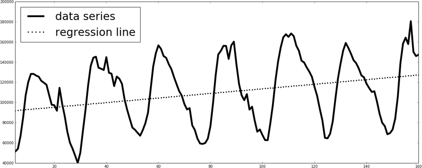
12 To be pedantic, autocorrelation is the correlation of the time series vector with the same vector shifted by some negative time delta.

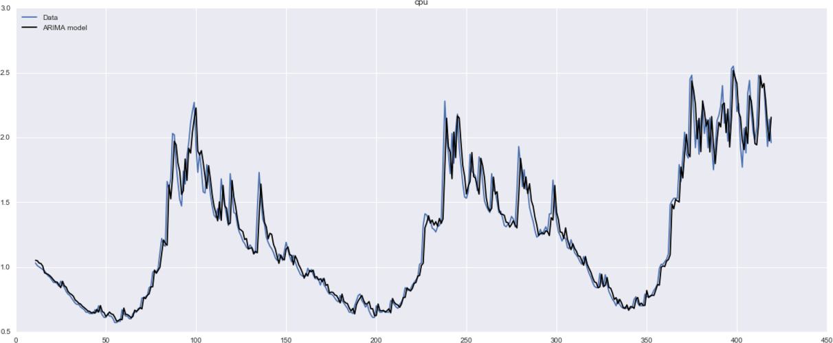
13 Robert Nau of Duke University provides a great, detailed resource for forecasting, ARIMA, and more.

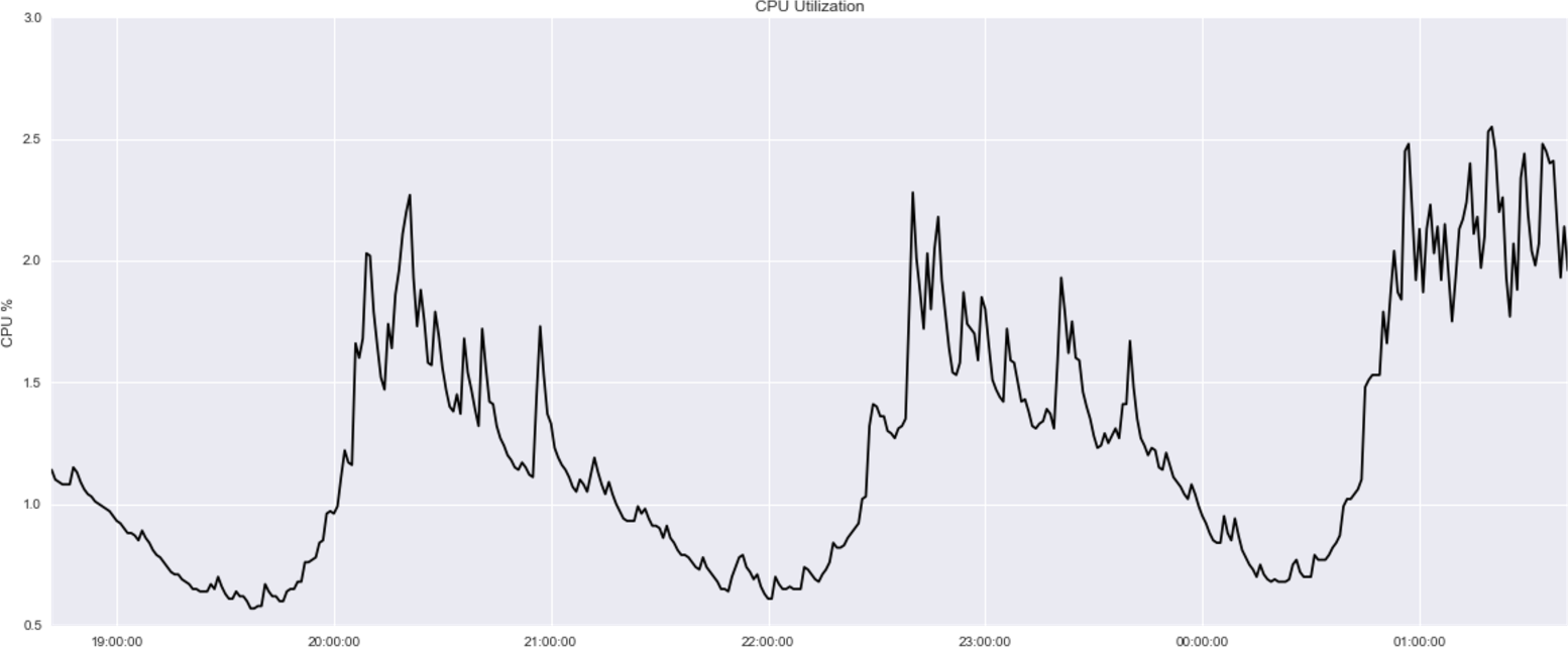
14 See chapter3/datasets/cpu-utilization in our code repository.

15 You can find documentation for PyFlux at http://www.pyflux.com/docs/arima.html?highlight=mle.

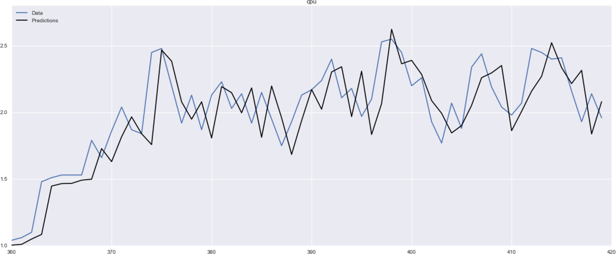
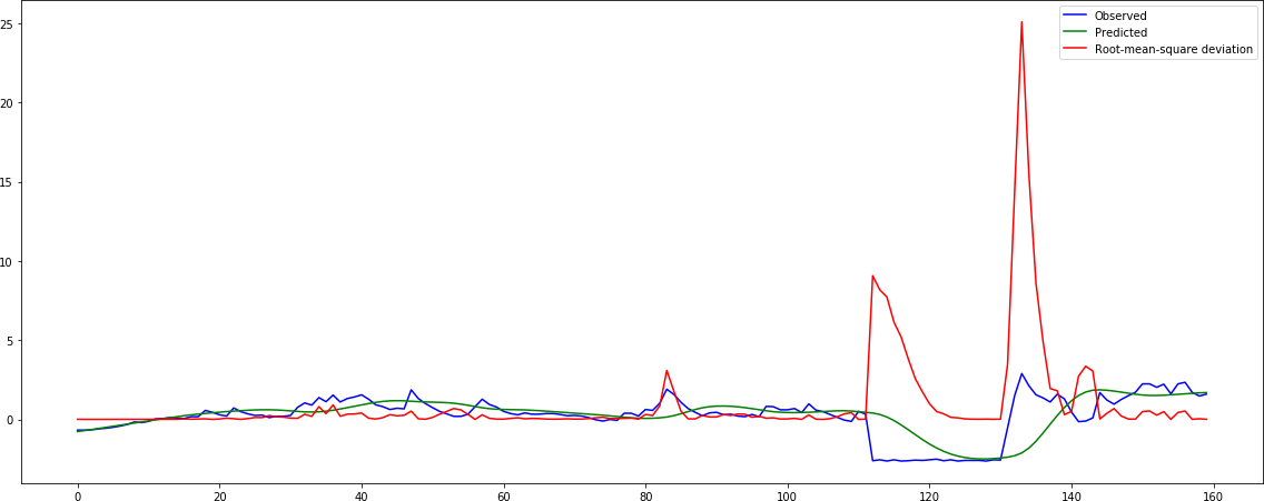
16 Full example code is given as a Python Jupyter notebook at chapter3/arima-forecasting.ipynb in our code repository.

17 ARIMAX is a slight modification of ARIMA that adds components originating from standard econometrics, known as explanatory variables, to the prediction models.

18 Sepp Hochreiter and Jürgen Schmidhuber, “Long Short-Term Memory,” Neural Computation 9 (1997): 1735–1780.

19 Alex Graves, “Generating Sequences with Recurrent Neural Networks”, University of Toronto (2014).

20 Neural networks are made up of layers of individual units. Data is fed into the input layer and predictions are produced from the output layer. In between, there can be an arbitrary number of hidden layers. In counting the number of layers in a neural network, a widely accepted convention is to not count the input layer. For example, in a six-layer neural network, we have one input layer, five hidden layers, and one output layer.

21 Full example code is given as a Python Jupyter notebook at chapter3/lstm-anomaly-detection.ipynb in our code repository.

22 Nitish Srivastava et al., “Dropout: A Simple Way to Prevent Neural Networks from Overfitting,” Journal of Machine Learning Research 15 (2014): 1929−1958.

23 Eamonn Keogh and Jessica Lin, “Clustering of Time-Series Subsequences Is Meaningless: Implications for Previous and Future Research,” Knowledge and Information Systems 8 (2005): 154–177.

24 This example can be found at chapter3/mad.py in our code repository.

25 The law of large numbers is a theorem that postulates that repeating an experiment a large number of times will produce a mean result that is close to the expected value.

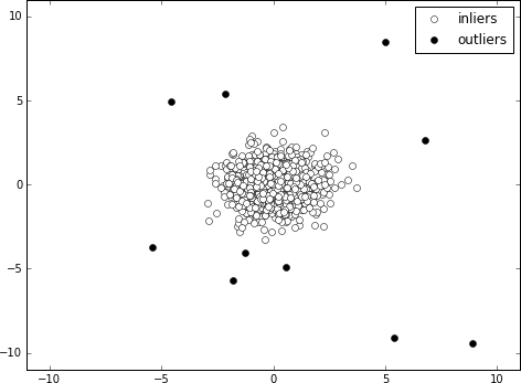
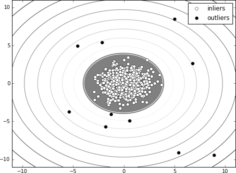
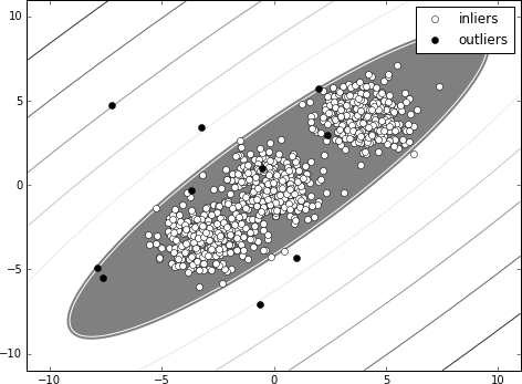
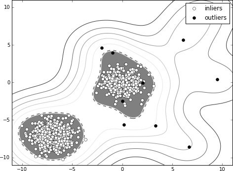
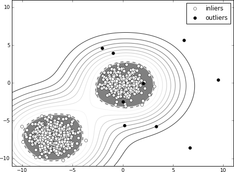
26 The full code can be found as a Python Jupyter notebook at chapter3/elliptic-envelope-fitting.ipynb in our code repository.

27 In statistics, robust is a property that is used to describe a resilience to outliers. More generally, the term robust statistics refers to statistics that are not strongly affected by certain degrees of departures from model assumptions.

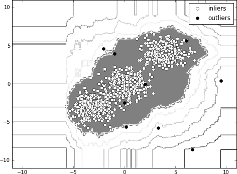
28 The full code can be found as a Python Jupyter notebook at chapter3/one-class-svm.ipynb in our code repository.

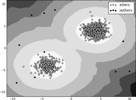
29 The full code can be found as a Python Jupyter notebook at chapter3/isolation-forest.ipynb in our code repository.

30 Alexandr Andoni and Piotr Indyk, “Nearest Neighbors in High-Dimensional Spaces,” in Handbook of Discrete and Computational Geometry, 3rd ed., ed. Jacob E. Goodman, Joseph O’Rourke, and Piotr Indyk (CRC Press).

31 The full code can be found as a Python Jupyter notebook at chapter3/local-outlier-factor.ipynb in our code repository.

32 In Chapter 7, we examine the details of dealing with explainability in machine learning in more depth.

33 Ryan Turner, “A Model Explanation System”, Black Box Learning and Inference NIPS Workshop (2015).