Spam Fighting: An Iterative Approach
As discussed earlier, the example of spam fighting is both one of the oldest problems in computer security and one that has been successfully attacked with machine learning. In this section, we dive deep into this topic and show how to gradually build up a sophisticated spam classification system using machine learning. The approach we take here will generalize to many other types of security problems, including but not limited to those discussed in later chapters of this book.
Consider a scenario in which you are asked to solve the problem of rampant email spam affecting employees in an organization. For whatever reason, you are instructed to develop a custom solution instead of using commercial options. Provided with administrator access to the private email servers, you are able to extract a body of emails for analysis. All the emails are properly tagged by recipients as either “spam” or “ham” (non-spam), so you don’t need to spend too much time cleaning the data.6
Human beings do a good job at recognizing spam, so you begin by implementing a simple solution that approximates a person’s thought process while executing this task. Your theory is that the presence or absence of some prominent keywords in an email is a strong binary indicator of whether the email is spam or ham. For instance, you notice that the word “lottery” appears in the spam data a lot, but seldom appears in regular emails. Perhaps you could come up with a list of similar words and perform the classification by checking whether a piece of email contains any words that belong to this blacklist.
The dataset that we will use to explore this problem is the 2007 TREC Public Spam Corpus. This is a lightly cleaned raw email message corpus containing 75,419 messages collected from an email server over a three-month period in 2007. One-third of the dataset is made up of spam examples, and the rest is ham. This dataset was created by the Text REtrieval Conference (TREC) Spam Track in 2007, as part of an effort to push the boundaries of state-of-the-art spam detection.
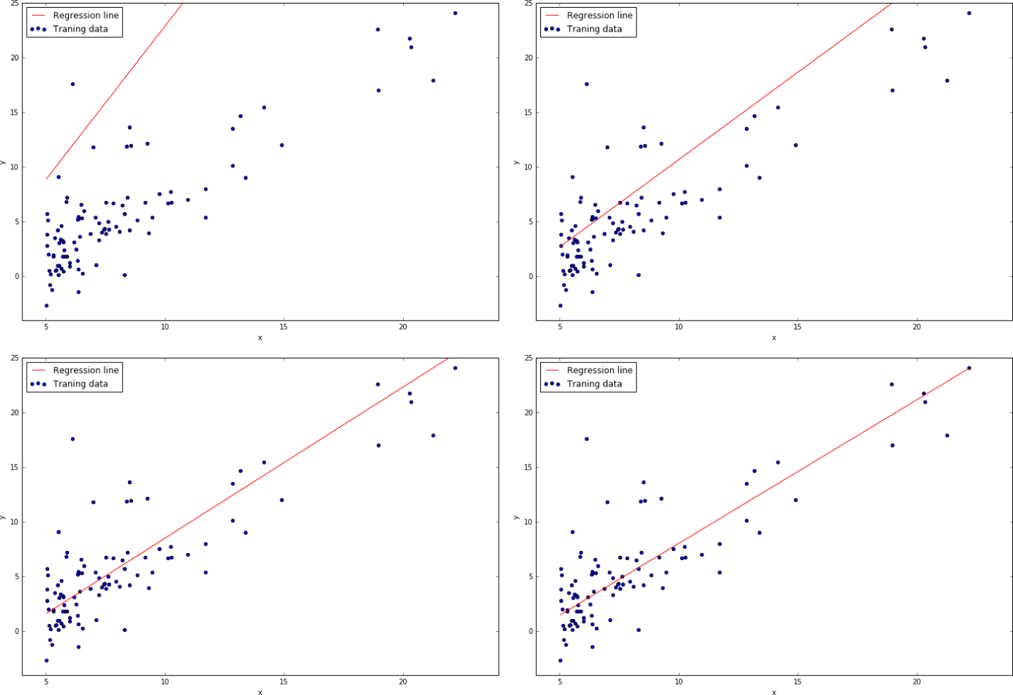
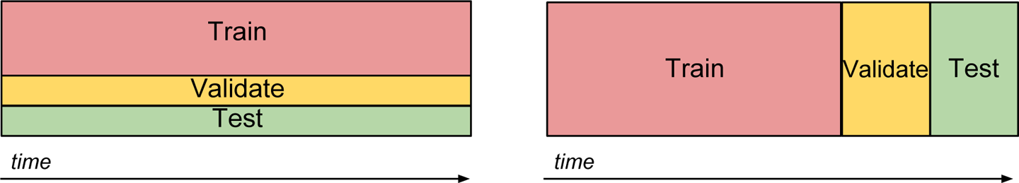
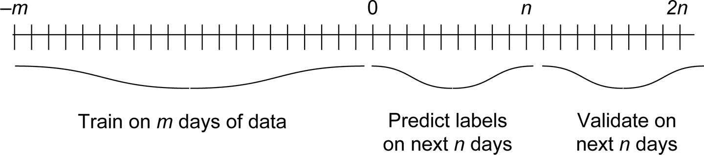
For evaluating how well different approaches work, we will go through a simple validation process.7 We split the dataset into nonoverlapping training and test sets, in which the training set consists of 70% of the data (an arbitrarily chosen proportion) and the test set consists of the remaining 30%. This method is standard practice for assessing how well an algorithm or model developed on the basis of the training set will generalize to an independent dataset.
The first step is to use the Natural Language Toolkit (NLTK) to remove morphological affixes from words for more flexible matching (a process called stemming). For instance, this would reduce the words “congratulations” and “congrats” to the same stem word, “congrat.” We also remove stopwords (e.g., “the,” “is,” and “are,”) before the token extraction process, because they typically do not contain much meaning. We define a set of functions8 to help with loading and preprocessing the data and labels, as demonstrated in the following code:9
import string
import email
import nltk

punctuations = list(string.punctuation)
stopwords = set(nltk.corpus.stopwords.words('english'))
stemmer = nltk.PorterStemmer()

# Combine the different parts of the email into a flat list of strings
def flatten_to_string(parts):
    ret = []
    if type(parts) == str:
        ret.append(parts)
    elif type(parts) == list:
        for part in parts:
            ret += flatten_to_string(part)
    elif parts.get_content_type == 'text/plain':
        ret += parts.get_payload()
    return ret

# Extract subject and body text from a single email file
def extract_email_text(path):
    # Load a single email from an input file
    with open(path, errors='ignore') as f:
        msg = email.message_from_file(f)
    if not msg:
        return ""

    # Read the email subject
    subject = msg['Subject']
    if not subject:
        subject = ""

    # Read the email body
    body = ' '.join(m for m in flatten_to_string(msg.get_payload())
                    if type(m) == str)
    if not body:
        body = ""

    return subject + ' ' + body

# Process a single email file into stemmed tokens
def load(path):
    email_text = extract_email_text(path)
    if not email_text:
        return []

    # Tokenize the message
    tokens = nltk.word_tokenize(email_text)

    # Remove punctuation from tokens
    tokens = [i.strip("".join(punctuations)) for i in tokens
              if i not in punctuations]

    # Remove stopwords and stem tokens
    if len(tokens) > 2:
        return [stemmer.stem(w) for w in tokens if w not in stopwords]
    return []
Next, we proceed with loading the emails and labels. This dataset provides each email in its own individual file (inmail.1, inmail.2, inmail.3, …), along with a single label file (full/index) in the following format:
spam   ../data/inmail.1
ham    ../data/inmail.2
spam   ../data/inmail.3
...
Each line in the label file contains the “spam” or “ham” label for each email sample in the dataset. Let’s read the dataset and build a blacklist of spam words now:10
import os

DATA_DIR = 'datasets/trec07p/data/'
LABELS_FILE = 'datasets/trec07p/full/index'
TRAINING_SET_RATIO = 0.7

labels = {}
spam_words = set()
ham_words = set()

# Read the labels
with open(LABELS_FILE) as f:
    for line in f:
        line = line.strip()
        label, key = line.split()
        labels[key.split('/')[-1]] = 1 if label.lower() == 'ham' else 0

# Split corpus into training and test sets
filelist = os.listdir(DATA_DIR)
X_train = filelist[:int(len(filelist)*TRAINING_SET_RATIO)]
X_test = filelist[int(len(filelist)*TRAINING_SET_RATIO):]

for filename in X_train:
    path = os.path.join(DATA_DIR, filename)
    if filename in labels:
        label = labels[filename]
        stems = load(path)
        if not stems:
            continue
        if label == 1:
            ham_words.update(stems)
        elif label == 0:
            spam_words.update(stems)
        else:
            continue

blacklist = spam_words - ham_words
Upon inspection of the tokens in blacklist, you might feel that many of the words are nonsensical (e.g., Unicode, URLs, filenames, symbols, foreign words). You can remedy this problem with a more thorough data-cleaning process, but these simple results should perform adequately for the purposes of this experiment:
greenback, gonorrhea, lecher, ...
Evaluating our methodology on the 22,626 emails in the testing set, we realize that this simplistic algorithm does not do as well as we had hoped. We report the results in a confusion matrix, a 2 × 2 matrix that gives the number of examples with given predicted and actual labels for each of the four possible pairs:
|
Predicted HAM |
Predicted SPAM |
Actual HAM |
6,772 |
714 |
Actual SPAM |
5,835 |
7,543 |
True positive: predicted spam + actual ham |
True negative: predicted ham + actual ham |
False positive: predicted spam + actual ham |
False negative: predicted ham + actual spam |
Converting this to percentages, we get the following:
|
Predicted HAM |
Predicted SPAM |
Actual HAM |
32.5% |
3.4% |
Actual SPAM |
28.0% |
36.2% |
Classification accuracy: 68.7% |
Ignoring the fact that 5.8% of emails were not classified because of preprocessing errors, we see that the performance of this naive algorithm is actually quite fair. Our spam blacklist technique has a 68.7% classification accuracy (i.e., total proportion of correct labels). However, the blacklist doesn’t include many words that spam emails use, because they are also frequently found in legitimate emails. It also seems like an impossible task to maintain a constantly updated set of words that can cleanly divide spam and ham. Maybe it’s time to go back to the drawing board.
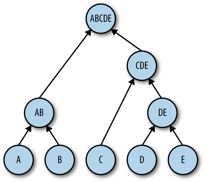
Next, you remember reading that one of the popular ways that email providers fought spam in the early days was to perform fuzzy hashing on spam messages and filter emails that produced a similar hash. This is a type of collaborative filtering that relies on the wisdom of other users on the platform to build up a collective intelligence that will hopefully generalize well and identify new incoming spam. The hypothesis is that spammers use some automation in crafting spam, and hence produce spam messages that are only slight variations of one another. A fuzzy hashing algorithm, or more specifically, a locality-sensitive hash (LSH), can allow you to find approximate matches of emails that have been marked as spam.
Upon doing some research, you come across datasketch, a comprehensive Python package that has efficient implementations of the MinHash + LSH algorithm11 to perform string matching with sublinear query costs (with respect to the cardinality of the spam set). MinHash converts string token sets to short signatures while preserving qualities of the original input that enable similarity matching. LSH can then be applied on MinHash signatures instead of raw tokens, greatly improving performance. MinHash trades the performance gains for some loss in accuracy, so there will be some false positives and false negatives in your result. However, performing naive fuzzy string matching on every email message against the full set of n spam messages in your training set incurs either O(n) query complexity (if you scan your corpus each time) or O(n) memory (if you build a hash table of your corpus), and you decide that you can deal with this trade-off:12,13
from datasketch import MinHash, MinHashLSH

# Extract only spam files for inserting into the LSH matcher
spam_files = [x for x in X_train if labels[x] == 0]

# Initialize MinHashLSH matcher with a Jaccard
# threshold of 0.5 and 128 MinHash permutation functions
lsh = MinHashLSH(threshold=0.5, num_perm=128)

# Populate the LSH matcher with training spam MinHashes
for idx, f in enumerate(spam_files):
    minhash = MinHash(num_perm=128)
    stems = load(os.path.join(DATA_DIR, f))
    if len(stems) < 2: continue
    for s in stems:
        minhash.update(s.encode('utf-8'))
    lsh.insert(f, minhash)
Now it’s time to have the LSH matcher predict labels for the test set:
def lsh_predict_label(stems):
    '''
    Queries the LSH matcher and returns:
        0 if predicted spam
        1 if predicted ham
       −1 if parsing error
    '''
    minhash = MinHash(num_perm=128)
    if len(stems) < 2:
        return −1
    for s in stems:
        minhash.update(s.encode('utf-8'))
    matches = lsh.query(minhash)
    if matches:
        return 0
    else:
        return 1
Inspecting the results, you see the following:
|
Predicted HAM |
Predicted SPAM |
Actual HAM |
7,350 |
136 |
Actual SPAM |
2,241 |
11,038 |
Converting this to percentages, you get:
|
Predicted HAM |
Predicted SPAM |
Actual HAM |
35.4% |
0.7% |
Actual SPAM |
10.8% |
53.2% |
Classification accuracy: 88.6% |
That’s approximately 20% better than the previous naive blacklisting approach, and significantly better with respect to false positives (i.e., predicted spam + actual ham). However, these results are still not quite in the same league as modern spam filters. Digging into the data, you realize that it might not be an issue with the algorithm, but with the nature of the data you have—the spam in your dataset just doesn’t seem all that repetitive. Email providers are in a much better position to make use of collaborative spam filtering because of the volume and diversity of messages that they see. Unless a spammer were to target a large number of employees in your organization, there would not be a significant amount of repetition in the spam corpus. You need to go beyond matching stem words and computing Jaccard similarities if you want a breakthrough.
By this point, you are frustrated with experimentation and decide to do more research before proceeding. You see that many others have obtained promising results using a technique called Naive Bayes classification. After getting a decent understanding of how the algorithm works, you begin to create a prototype solution. Scikit-learn provides a surprisingly simple class, sklearn.naive_bayes.MultinomialNB, that you can use to generate quick results for this experiment. You can reuse a lot of the earlier code for parsing the email files and preprocessing the labels. However, you decide to try passing in the entire email subject and plain text body (separated by a new line) without doing any stopword removal or stemming with NLTK. You define a small function to read all the email files into this text form:14,15
def read_email_files():
    X = []
    y = []
    for i in xrange(len(labels)):
        filename = 'inmail.' + str(i+1)
        email_str = extract_email_text(os.path.join(DATA_DIR, filename))
        X.append(email_str)
        y.append(labels[filename])
    return X, y
Then you use the utility function sklearn.model_selection.train_test_split() to randomly split the dataset into training and testing subsets (the argument random_state=123 is passed in for the sake of result reproducibility):
from sklearn.model_selection import train_test_split

X, y = read_email_files()

X_train, X_test, y_train, y_test, idx_train, idx_test = \
    train_test_split(X, y, range(len(y)),
    train_size=TRAINING_SET_RATIO, random_state=2)
Now that you have prepared the raw data, you need to do some further processing of the tokens to convert each email to a vector representation that MultinomialNB accepts as input.
One of the simplest ways to convert a body of text into a feature vector is to use the bag-of-words representation, which goes through the entire corpus of documents and generates a vocabulary of tokens used throughout the corpus. Every word in the vocabulary comprises a feature, and each feature value is the count of how many times the word appears in the corpus. For example, consider a hypothetical scenario in which you have only three messages in the entire corpus:
tokenized_messages: {
    'A': ['hello', 'mr', 'bear'],
    'B': ['hello', 'hello', 'gunter'],
    'C': ['goodbye', 'mr', 'gunter']
}

# Bag-of-words feature vector column labels:
# ['hello', 'mr', 'doggy', 'bear', 'gunter', 'goodbye']
vectorized_messages: {
    'A': [1,1,0,1,0,0],
    'B': [2,0,0,0,1,0],
    'C': [0,1,0,0,1,1]
}
Even though this process discards seemingly important information like the order of words, content structure, and word similarities, it is very simple to implement using the sklearn.feature_extraction.CountVectorizer class:
from sklearn.feature_extraction.text import CountVectorizer

vectorizer = CountVectorizer()
X_train_vector = vectorizer.fit_transform(X_train)
X_test_vector = vectorizer.transform(X_test)
You can also try using the term frequency/inverse document frequency (TF/IDF) vectorizer instead of raw counts. TF/IDF normalizes raw word counts and is in general a better indicator of a word’s statistical importance in the text. It is provided as sklearn.feature_extraction.text.TfidfVectorizer.
Now you can train and test your multinomial Naive Bayes classifier:
from sklearn.naive_bayes import MultinomialNB
from sklearn.metrics import accuracy_score

# Initialize the classifier and make label predictions
mnb = MultinomialNB()
mnb.fit(X_train_vector, y_train)
y_pred = mnb.predict(X_test_vector)

# Print results
print('Accuracy {:.3f}'.format(accuracy_score(y_test, y_pred)))

> Accuracy: 0.956
An accuracy of 95.6%—a whole 7% better than the LSH approach!16 That’s not a bad result for a few lines of code, and it’s in the ballpark of what modern spam filters can do. Some state-of-the-art spam filters are in fact actually driven by some variant of Naive Bayes classification. In machine learning, combining multiple independent classifiers and algorithms into an ensemble (also known as stacked generalization or stacking) is a common way of taking advantage of each method’s strengths. So, you can imagine how a combination of word blacklists, fuzzy hash matching, and a Naive Bayes model can help to improve this result.
Alas, spam detection in the real world is not as simple as we have made it out to be in this example. There are many different types of spam, each with a different attack vector and method of avoiding detection. For instance, some spam messages rely heavily on tempting the reader to click links. The email’s content body thus might not contain as much incriminating text as other kinds of spam. This kind of spam then might try to circumvent link-spam detection classifiers using complex methods like cloaking and redirection chains. Other kinds of spam might just rely on images and not rely on text at all.
For now, you are happy with your progress and decide to deploy this solution. As is always the case when dealing with human adversaries, the spammers will eventually realize that their emails are no longer getting through and might act to avoid detection. This response is nothing out of the ordinary for problems in security. You must constantly improve your detection algorithms and classifiers and stay one step ahead of your adversaries.
In the following chapters, we explore how machine learning methods can help you avoid having to be constantly engaged in this whack-a-mole game with attackers, and how you can create a more adaptive solution to minimize constant manual tweaking.