Chapter 7. Production Systems

Up to this point in the book, we have focused our discussion on implementing machine learning algorithms for security in isolated lab environments. After you have proven that the algorithm works, the next step will likely be to get the software ready for production. Deploying machine learning systems in production comes with an entirely different set of challenges and concerns that you might not have had to deal with during the experimentation and development phases. What does it take to engineer truly scalable machine learning systems? How do we manage the efficacy, reliability, and relevance of web-scale security services in dynamic environments where change is constant? This chapter is dedicated to security and data at scale, and we will address these questions and more.

Let’s begin by concretely defining what it means for such systems to be production ready, deployable, and scalable.

Defining Machine Learning System Maturity and Scalability

Instead of floating around abstract terms for describing the quality of code in production, it will benefit the discussion to detail some characteristics that mature and scalable machine learning systems should have. The following list of features describes an ideal machine learning system, regardless of whether it is related to security; the items highlighted in bold are especially important for security machine learning systems. The list also serves as an outline for the remainder of this chapter, so if there is any item you are particularly curious about, you can jump to the corresponding section to learn more. We will examine the following topics:

  • Data Quality

    • Unbiased data

    • Verifiable ground truth

    • Sound treatment of missing data

  • Model Quality

    • Efficient hyperparameter optimization

    • A/B testing of models

    • Timely feedback loops

    • Repeatable results

    • Explainable results

  • Performance

    • Low-latency training and predictions

    • Scalability (i.e., can it handle 10 times the traffic?)

    • Automated and efficient data collection

  • Maintainability

    • Checkpointing and versioning of models

    • Smooth model deployment process

    • Graceful degradation

    • Easily tunable and configurable

    • Well documented

  • Monitoring and Alerting

    • System health/performance monitoring (i.e., is it running?)

    • System efficacy monitoring (i.e., precision/recall)

    • Monitoring data distributions (e.g., user behavior changing or adversaries adapting)

  • Security and Reliability

    • Robust in adversarial contexts

    • Data privacy safeguards and guarantees

This is a long list, but not all the listed points are applicable to all types of systems. For instance, explainable results might not be relevant for an online video recommendation system because there are typically no accountability guarantees and the cost of a missed prediction is low. Systems that do not naturally attract malicious tampering might not have a strong incentive to devote resources to making models robust to adversarial activity.

What’s Important for Security Machine Learning Systems?

Security machine learning applications must meet an especially stringent set of requirements before it makes sense to put them into production. Right from the start, almost all such systems have high prediction accuracy requirements because of the unusually high cost of getting something wrong. An error rate of 0.001 (99.9% prediction accuracy) might be good enough for a sales projection model that makes 100 predictions per day—on average, only 1 wrong prediction will be made every 10 days. On the other hand, a network packet classifier that inspects a million TCP packets every minute will be misclassifying 1,000 of those packets each minute. Without separate processes in place to filter out these false positives and false negatives, an error rate of 0.001 is untenable for such a system. If every false positive has to be manually triaged by a human analyst, the cost of operation will be too high. For every false negative, or missed detection, the potential consequences can be dire: the entire system can be compromised.

All of the properties of mature and scalable machine learning systems that we just listed are important, but the highlighted ones are especially critical to the success of security machine learning systems.

Let’s dive into the list of qualities and look at more specific techniques for developing scalable, production-quality security machine learning systems. In the following sections, we examine each issue that either is commonly overlooked or poses a challenge for the use of machine learning in security. For each, we first describe the problem or goal and explain why it is important. Next, we discuss ways to approach system design that can help achieve the goal or mitigate the problem.

Data Quality

The quality of a machine learning system’s input data dictates its success or failure. When training an email spam classifier using supervised learning, feeding an algorithm training data that contains only health and medicine advertising spam emails will not result in a balanced and generalizable model. The resulting system might be great at recognizing unsolicited emails promoting weight-loss medication, but it will likely be unable to detect adult content spam.

Problem: Bias in Datasets

Well-balanced datasets are scarce, and using unbalanced datasets can result in bias that is difficult to detect. For example, malware datasets are rarely varied enough to cover all different types of malware that a system might be expected to classify. Depending on what was collected in honeypots, the dates the samples were collected, the source of nonmalicious binaries, and so on, there is often significant bias in these datasets.

Machine learning algorithms rely on datasets fed into algorithms to execute the learning task. We use the term population to refer to the universe of data whose characteristics and/or behavior the algorithm should model. For example, suppose that we want to devise a machine learning algorithm to separate all phishing emails from all benign emails; in this case, the population refers to all emails that have existed in the past, present, and future.

Because it is typically impossible to collect samples from the entire population, datasets are created by drawing from sources that produce samples belonging to the population. For example, suppose that a convenient dataset for enterprise X is emails from its corporate email server for the month of March. Using this dataset eventually produces a classifier that performs very well for enterprise X, but there is no guarantee that it will continue to perform well as time progresses or if brought to another company. Specifically, the phishing emails received by a different enterprise Y also belong to the population, but they might have very different characteristics that are not exhibited in enterprise X, in which case it is unlikely that the classifier will produce good results on enterprise Y’s emails. Suppose further that the phishing samples within the dataset are mostly made up of tax scam and phishing emails, given that March and April happen to be tax season in the United States. Unless you take special care, the model might not learn the characteristics of other types of phishing emails and is not likely to perform well in a general test scenario. Because the goal was to build a general phishing classifier that worked well on all emails, the dataset used to train it was inadequately drawn from the population. This classifier is a victim of selection bias and exclusion bias1 because of the temporal and contextual effects that contributed to the selection of the particular dataset used to train the classifier.

Selection bias and exclusion bias are common forms of bias that can be caused by flawed data collection flows. These forms of bias are introduced by the systematic and improper selection or exclusion of data from the population intended to be analyzed, resulting in datasets that have properties and a distribution that are not representative of the population.

Observer bias, or the observer-expectancy effect, is another common type of bias caused by errors in human judgment or human-designed processes. Software binary feature extraction processes might be biased toward certain behavior exhibited by the binaries that human analysts have been trained to look out for; for example, DNS queries to command-and-control (C&C) servers. As a result, the detection and collection mechanisms in such pipelines might miss out on other equally telling but less commonly exhibited malicious actions, such as unauthorized direct memory accesses. This bias causes imperfect data and incorrect labels assigned to samples, affecting the accuracy of the system.

Problem: Label Inaccuracy

When doing supervised learning, mislabeled data will cause machine learning algorithms to lose accuracy. The problem is exacerbated if the validation datasets are also wrongly labeled. Development-time validation accuracy can look promising, but the model will likely not perform as expected when fed with real data in production. The problem of inaccurate labels is commonly seen when crowdsourcing is used without proper safeguards. User feedback or experts making decisions on incomplete information can also result in mislabeled data. Mislabeled data can seriously interfere with the learning objectives of algorithms unless you recognize and deal with it.

Checking the correctness of labels in a dataset often requires expensive human expert resources. It can take hours for an experienced security professional to check whether a binary flagged by your system actually carries out malicious behavior. Even doing random subset validation on datasets can still be expensive.

Solutions: Data Quality

There are many different causes of data quality problems, and there are few quick and easy remedies. The most critical step in dealing with data quality issues in security machine learning systems is to recognize that the problem exists. Class imbalance (as discussed in Chapter 5) is a manifestation of data bias in which the number of samples of one class of data is vastly smaller (or larger) than the number of samples of another class. Class imbalance is a fairly obvious problem that we can find during the exploration or training phase and alleviate with oversampling and undersampling, as discussed earlier. However, there are other forms of data bias and inaccuracies that can be subtler yet equally detrimental to model performance. Detecting selection bias and observer bias is challenging, especially when the problem results from implementers’ and designers’ blind spots. Spending time and resources to understand the exact goals of the problem and the nature of the data is the only way to determine if there are important aspects of the data that your datasets are unable to capture.

In some cases, you can avoid data quality issues by carefully defining the scope of the problem. For instance, systems that claim to detect all kinds of phishing emails will have a challenging time generating a representative training dataset. However, if the scope of the problem is narrowed to the most important problem an organization is facing—for example, detecting phishing emails that attempt to clickjack2 the user—it will be easier to gather more focused data for the problem.

Inaccurate labels caused by errors in human labeling can be made less likely by involving multiple independent annotators in the labeling process. You can use statistical measures (such as the Fleiss’ kappa3) to assess the reliability of agreement between the annotations of multiple labelers and weed out incorrect labels. Assuming that labels were not assigned in mischief or malice by the annotators, the level of disagreement between human annotators for a particular sample’s label is also often used as the upper bound of the likelihood a machine learning classifier is able to predict the correct label for the sample. For example, imagine that two independent annotators label an email as spam, and another two think it is ham. This indicates that the sample might be ambiguous, given that even human experts cannot agree on its label. Machine learning classifiers will not be likely to perform well on such samples, and it is best to exclude such samples from the dataset to avoid confounding the learning objectives of the algorithm.

If you know that the dataset has noisy labels but it is impossible or too costly to weed out the inaccuracies, increasing regularization parameters to deliberately disincentivize overfitting at the expense of prediction accuracy can be a worthwhile trade-off. Overfitting a model to a noisily labeled dataset can be catastrophic and result in a “garbage-in, garbage-out” scenario.

Problem: Missing Data

Missing data is one of the most common problems that you will face when working with machine learning. It is very common for datasets to have rows with missing values. These can be caused by errors in the data collection process, but datasets can also contain missing data by design. For instance, if a dataset is collected through surveys with human respondents, there may be some optional questions some people choose not to answer. This causes null values to end up in the dataset, causing problems when it comes time for analysis. Some algorithms will refuse to classify a row with null values, rendering any such row useless even if it contains valid data in most columns. Others will use default values in the input or output, which can lead to erroneous results.

A common mistake is to fill in the blanks with sentinel values; that is, dummy data of the same format/type as the rest of the column that signals to the operator that this value was originally blank, such as 0 or −1 for numeric values. Sentinel values pollute the dataset by inserting data that is not representative of the original population from which the samples are drawn. It might be obvious to you that 0 or −1 is not a valid value for a particular column, but it will in general not be obvious to your algorithm. The degree to which sentinel values can negatively affect classification results depends on the particular machine learning algorithm used.

Solutions: Missing Data

Let’s illustrate this problem with an example4 and experiment with some solutions. Our example dataset is a database containing records of 1,470 employees in an organization, past and present. The dataset, presented in Table 7-1, has four columns: “TotalWorkingYears,” “MonthlyIncome,” “Overtime,” and “DailyRate.” The “Label” indicates whether the employee has left the organization (with 0 indicating that the employee is still around).

What we are attempting to predict with this dataset is whether an employee has left (or is likely to leave), given the other four features. The “Overtime” feature is binary, and the other three features are numerical. Let’s process the dataset and attempt to classify it with a decision tree classifier, as we have done in earlier chapters. We first define a helper function that builds a model and returns its accuracy on a test set:

def build_model(dataset, test_size=0.3, random_state=17):
    # Split data into training and test sets
    X_train, X_test, y_train, y_test = train_test_split(
        dataset.drop('Label', axis=1), dataset.Label,
        test_size=test_size, random_state=random_state)

    # Fit a decision tree classifier
    clf = DecisionTreeClassifier(
        random_state=random_state).fit(X_train, y_train)

    # Compute the accuracy
    y_pred = clf.predict(X_test)
    return accuracy_score(y_test, y_pred)

Now let’s try building a model on the entire dataset:

# Read the data into a DataFrame
df = pd.read_csv('employee_attrition_missing.csv')
build_model(df)

At this point, scikit-learn throws an error:

> ValueError: Input contains NaN, infinity or a value too large for
      dtype('float32').

It appears that some of the values in this dataset are missing. Let’s inspect the DataFrame:

df.head()
Table 7-1. Sample rows drawn from employee attrition dataset
TotalWorkingYears MonthlyIncome Overtime DailyRate Label

0

NaN

6725

0

498.0

0

1

12.0

2782

0

NaN

0

2

9.0

2468

0

NaN

0

3

8.0

5003

0

549.0

0

4

12.0

8578

0

NaN

0

We see from Table 7-1 that there are quite a few rows that have “NaN” values for the “TotalWorkingYears” and “DailyRate” columns.

There are five methods that you can use to deal with missing values in datasets:

  1. Discard rows with any missing values (without replacement).

  2. Discard columns that have missing values.

  3. Fill in missing values by collecting more data.

  4. Fill in missing values with zeroes or some other “indicator” value.

  5. Impute the missing values.

Method 1 works if not many rows have missing values and you have an abundance of data points. For example, if only 1% of your samples are missing data, it can be acceptable to completely remove those rows. Method 2 is useful if the features for which some rows have missing values are not strong features for learning. For example, if only the “age” column has missing values in a dataset, and the age feature does not seem to contribute to the learning algorithm much (i.e., removing the feature does not cause a significant decrease in prediction accuracy), it can be acceptable to completely exclude the column from the learning process. Methods 1 and 2 are simple, but most operators seldom find themselves in positions in which they have enough data or features that they can discard rows or columns without affecting performance.

Let’s see what fraction of our samples have missing data. We can drop rows containing any “NaN” values with the function pandas.DataFrame.dropna():

num_orig_rows = len(df)
num_full_rows = len(df.dropna())

(num_orig_rows - num_full_rows)/float(num_orig_rows)

> 0.5653061224489796

More than half of the rows have at least one value missing and two out of four columns have values missing—not promising! Let’s see how methods 1 and 2 perform on our data:

df_droprows = df.dropna()
build_model(df_droprows)

> 0.75520833333333337

df_dropcols = df[['MonthlyIncome','Overtime','Label']]
build_model(df_dropcols)

> 0.77324263038548757

Dropping rows with missing values gives a 75.5% classification accuracy, whereas dropping columns with missing values gives an accuracy of 77.3%. Let’s see if we can do better.

Methods 3 and 4 attempt to fill in the gaps instead of discarding the “faulty” rows. Method 3 gives the highest-quality data, but is often unrealistic and expensive. For this example, it would be too expensive to chase each employee down just to fill in the missing entries. We also cannot possibly generate more data unless more employees join the company.

Let’s try method 4, filling in all missing values with a sentinel value of −1 (because all of the data is nonnegative, −1 is a good indicator of missing data):

# Fill all NaN values with −1
df_sentinel = df.fillna(value=-1)
build_model(df_sentinel)

> 0.75283446712018143

This approach gives us a 75.3% classification accuracy—worse than simply dropping rows or columns with missing data! We see here the danger of naively inserting values without regard to what they might mean.

Let’s compare these results to what method 5 can do. Imputation refers to the act of replacing missing values with intelligently chosen values that minimize the effect of this filler data on the dataset’s distribution. In other words, we want to ensure that the values that we fill the gaps with do not pollute the data significantly. The best way to select a value for filling the gaps is typically to use the mean, median, or most frequently appearing value (mode) of the column. Which method to choose depends on the nature of the dataset. If the dataset contains many outliers—for example, if 99% of “DailyRate” values are below 1,000 and 1% are above 100,000—imputing by mean would not be suitable.

Scikit-learn provides a convenient utility for imputing missing values: sklearn.preprocessing.Imputer. Let’s use this to fill in all the missing values with the respective means for each of the columns containing missing data:

from sklearn.preprocessing import Imputer

imp = Imputer(missing_values='NaN', strategy='mean', axis=0)

# Create a new DataFrame with the dataset transformed by the imputer
df_imputed = pd.DataFrame(imp.fit_transform(df),
                          columns=['TotalWorkingYears', 'MonthlyIncome',
                                   'OverTime', 'DailyRate', 'Label'])
build_model(df_imputed)

> 0.79365079365079361

Instantly, the classification accuracy increases to 79.4%. As you can guess, imputation is often the best choice for dealing with missing values.

Model Quality

Trained models form the core intelligence of machine learning systems. But without safeguards in place to ensure the quality of these models, the results they produce will be suboptimal. Models can take on different forms depending on the machine learning algorithm used, but they are essentially data structures containing the parameters learned during the algorithm’s training phase. For instance, a trained decision tree model contains all of the splits and values at each node, whereas a trained k-nearest neighbors (k-NN) classification model (naively implemented5 or ball trees6) is in fact the entire training dataset.

Model quality is not only important during the initial training and deployment phase. You must also take care as your system and the adversarial activity it faces evolve; regular maintenance and reevaluation will ensure that it does not degrade over time.

Problem: Hyperparameter Optimization

Hyperparameters are machine learning algorithm parameters that are not learned during the regular training process. Let’s look at some examples of tunable hyperparameters for the DecisionTreeClassifier in scikit-learn:

from sklearn import tree
classifier = tree.DecisionTreeClassifier(max_depth=12,
                                         min_samples_leaf=3,
                                         max_features='log2')

In the constructor of the classifier, we specify that the max_depth that the tree should grow to is 12. If this parameter is not specified, the default behavior of this implementation is to split nodes until all leaves are pure (only contain samples belonging to a single class) or, if the min_samples_split parameter is specified, to stop growing the tree when all leaf nodes have fewer than min_samples_split samples in them. We also specify min_samples_leaf=3, which means that the algorithm should ensure that there are at least three samples in a leaf node. max_features is set to log2, which indicates to the classifier that the maximum number of features it should consider when looking for the best split of a node is the base-2 logarithm of the number of features in the data. If you do not specify max_features, it defaults to the number of features. You can find the full list of tunable hyperparameters for any classifier in the documentation. If this looks intimidating to you, you are not alone.

Hyperparameters typically need to be chosen before commencing the training phase. But how do you know what to set the learning rate to? Or how many hidden layers in a deep neural network will give the best results? Or what value of k to use in k-means clustering? These seemingly arbitrary decisions can have a significant impact on a model’s efficacy. Novice practitioners typically try to avoid the complexity by using the default values provided by the machine learning library. Many mature machine learning libraries (including scikit-learn) do provide thoughtfully chosen default values that are adequate for the majority of use cases. Nevertheless, it is not possible for a set of hyperparameters to be optimal in all scenarios. A large part of your responsibility as a machine learning engineer is to understand the algorithms you use well enough to find the optimal combination of hyperparameters for the problem at hand. Because of the huge parameter space, this process can be expensive and slow, even for machine learning experts.

Solutions: Hyperparameter Optimization

Hyperparameters are a fragile component of machine learning systems because their optimality can be affected by small changes in the input data or other parts of the system. The problem can be naively approached in a “brute-force” fashion, by training different models using all different combinations of the algorithm’s hyperparameters, and then selecting the set of hyperparameters that results in the best-performing model.

Hyperparameter optimization is most commonly done using a technique called grid search, an exhaustive sweep through the hyperparameter space of a machine learning algorithm. By providing a metric for comparing how well each classifier performs with different combinations of hyperparameter values, the optimal configuration can be found. Even though this operation is computationally intensive, it can be easily parallelized because each different configuration of hyperparameter values can be independently computed and compared. Scikit-learn provides a class called sklearn.model_selection.GridSearchCV that implements this feature.

Let’s look at a short example of using a support vector machine to solve a digit classification problem—but instead of the commonly used MNIST data we’ll use a smaller and less computationally demanding dataset included in the scikit-learn digits dataset, adapted from the Pen-Based Recognition of Handwritten Digits Data Set. Before doing any hyperparameter optimization, it is good practice to establish a performance baseline with the default hyperparameters:

from sklearn import svm, metrics
from sklearn.model_selection import train_test_split
from sklearn.datasets import fetch_mldata, load_digits

# Read dataset and split into test/train sets
digits = load_digits()
n_samples = len(digits.images)
data = digits.images.reshape((n_samples, 1))
X_train, X_test, y_train, y_test = train_test_split(
    data, digits.target, test_size=0.3, random_state=0)

# Train SVC classifier, then get prediction and accuracy
classifier = svm.SVC()
classifier.fit(X_train, y_train)
predicted = classifier.predict(X_test)
print("Accuracy: %.3f" % metrics.accuracy_score(y_test, predicted))

> Accuracy: 0.472

An accuracy of 47.2% is pretty poor. Let’s see if tuning hyperparameters can give us a boost:

from sklearn.svm import SVC
from sklearn.model_selection import GridSearchCV

# Define a dictionary containing all hyperparameter values to try
hyperparam_grid = {
    'kernel': ('linear', 'rbf'),
    'gamma': [0.00001, 0.0001, 0.001, 0.01, 0.1, 1],
    'C': [1, 3, 5, 7, 9]
}

# Perform grid search with desired hyperparameters and classifier
classifier = GridSearchCV(svc, hyperparam_grid)
classifier.fit(X_train, y_train)

The hyperparam_grid dictionary passed into the GridSearchCV constructor along with the svc estimator object contains all of the hyperparameter values that we want the grid search algorithm to consider. The algorithm then builds 60 models, one for each possible combination of hyperparameters, and chooses the best one:

print('Best Kernel: %s' % classifier.best_estimator_.kernel)
print('Best Gamma: %s' % classifier.best_estimator_.gamma)
print('Best C: %s' % classifier.best_estimator_.C)

> Best Kernel: rbf
> Best Gamma:  0.001
> Best C:      3

The default values provided by the sklearn.svm.SVC class are kernel='rbf', gamma=1/n_features (for this dataset, n_features=64, so gamma=0.015625), and C=1. Note that the gamma and C proposed by GridSearchCV are different from the default values. Let’s see how it performs on the test set:

predicted = classifier.predict(X_test)
print("Accuracy: %.3f" % metrics.accuracy_score(y_test, predicted))

> Accuracy: 0.991

What a dramatic increase! Support vector machines are quite sensitive to their hyperparameters, especially the gamma kernel coefficient, for reasons which we will not go into here.

Note

GridSearchCV can take quite some time to run because it is training a separate SVC classifier for each combination of hyperparameter values provided in the grid. Especially when dealing with larger datasets, this process can be very expensive. Scikit-learn provides more optimized hyperparameter optimization algorithms such as sklearn.model_selection.RandomizedSearchCV that can return results more quickly.

Even for algorithms that have only a few hyperparameters, grid search is a very time- and resource-intensive way to solve the problem because of combinatorial explosion. Taking this naive approach as a performance baseline, we now consider some ways to optimize this process:

1) Understand the algorithm and its parameters well

Having a good understanding of the underlying algorithm and experience in implementation can guide you through the iterative process of manual hyperparameter optimization and help you to avoid dead ends. However, even if you are new to the field, the tuning process does not need to be completely blind. Visualizations of the training results can usually prompt adjustments of hyperparameters in certain directions and/or in magnitude. Let’s take the classic example of a neural network for classifying digits (from 0 to 9) from the MNIST image dataset7 of individual handwritten digits. The model we are using is a fully connected five-layer neural network implemented in TensorFlow. Using the visualization tool TensorBoard included in the standard distribution of TensorFlow, we plot a graph of the cross_entropy loss:

cross_entropy = tf.nn.softmax_cross_entropy_with_logits(
    logits=Ylogits, labels=Y_)
cross_entropy = tf.reduce_mean(cross_entropy)*100
tf.summary.scalar('cross_entropy', cross_entropy)

Figure 7-1 shows the result.

mlas 0701
Figure 7-1. TensorBoard scalar plot of training and test cross_entropy loss (log scale)

Observing the training and test cross_entropy loss over 10,000 epochs in Figure 7-1, we note an interesting dichotomy in the two trends. The training is performed on 55,000-digit samples and the testing is done on a static set of 10,000-digit samples. After each epoch, the cross_entropy loss is separately calculated on the training dataset (used to train the network) and the test dataset (which is not accessible to the network during the training phase). As expected, the training loss approaches zero over more training epochs, indicating that the network gradually performs better as it spends more time learning. The test loss initially follows a similar pattern to the training loss, but after about 2,000 epochs begins to trend upward. This is usually a clear sign that the network is overfitting to the training data. If you have dealt with neural networks before, you will know that dropout8 is the de facto way to perform regularization and deal with overfitting. Applying a dropout factor to the network will fix the upward trend of the test loss. By iteratively selecting different values of dropout on the network, you can then use this plot to find the hyperparameter value that reduces overfitting without sacrificing too much accuracy.

2) Mimic similar models

Another common way to solve the hyperparameter cold-start problem is to research previous similar work in the area. Even if the problem might not be of exactly the same nature, copying hyperparameters from other work while understanding why those choices were made can save you a lot of time because someone else has already put in the work to solve a similar problem. For example, it might take 10 iterations of experimentation to find out that 0.75 is the optimal dropout value to use for your MNIST classifier network, but looking at the values used to solve the MNIST problem in previously published work using a similar neural network could reduce your hyperparameter optimization time.

3) Don’t start tuning parameters too early

If you are resource constrained, don’t fret over hyperparameters. Only worry about the parameters when you suspect that they might be the cause of a problem in your classifier. Starting with the simplest configurations and watching out for potential improvements to make along the way is generally a good practice to follow.

Note

AutoML is a field of research that aims to automate the training and tuning of machine learning systems, including the process of hyperparameter optimization. In principle, AutoML tools can select the best algorithm for a task, perform an optimal architecture search for deep neural nets, and analyze the importance of hyperparameters to the prediction result. Though still very much in the research phase, AutoML is definitely an area to watch.

Feature: Feedback Loops, A/B Testing of Models

Because security machine learning systems have such a low tolerance for inaccuracies, every bit of user feedback needs to be taken into account to improve system efficacy as much as possible. For example, an anomaly detection system that raises too many false positive alerts to security operations personnel should take advantage of the correct labels given by human experts during the alert triaging phase to retrain and improve the model.

Long-running machine learning systems often also fall into the predicament of concept drift (also known as “model rot”), in which a model that originally yielded good results deteriorates over time. This is often an effect of changing properties of the input data due to external effects, and machine learning systems need to be flexible enough to adapt to such changes.

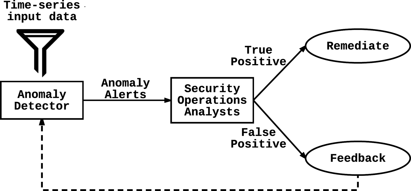
The first step to system flexibility is to detect model rot before it cripples the system by producing wrong or nonsensical output. Feedback loops are a good way to not only detect when the model is deteriorating but also gather labeled training data for continuously improving the system. Figure 7-2 presents a simple anomaly detection system with an integrated feedback loop.

mlas 0702
Figure 7-2. Anomaly detection system with feedback loop

The dashed line in Figure 7-2 indicates the information channel that security operations analysts are able to use to give expert feedback to the system. False positives produced by the detector will be flagged by human experts, who then can make use of this feedback channel to indicate to the system that it made a mistake. The system then can convert this feedback into a labeled data point and use it for further training. Feedback loops are immensely valuable because the labeled training samples they produce represent some of the most difficult predictions that the system has to make, which can help ensure that the system does not make similar mistakes in the future. Note that retraining with feedback may cause overfitting; you should take care to integrate this feedback with appropriate regularization. Feedback loops can also pose a security risk if the security operations analysts are not trusted personnel or if the system is somehow hijacked to provide malicious feedback. This will result in adversarial model poisoning; for example, red herring attacks, which will cause the model to learn from mislabeled data and performance to rapidly degrade. In Chapter 8, we discuss mitigation strategies for situations in which trust cannot be guaranteed within the system.

A/B testing, also known as split testing, refers to a randomized controlled experiment designed to understand how system variants affect metrics. Most large websites today run hundreds or even thousands of A/B tests simultaneously, as different product groups seek to optimize different metrics. The standard procedure for an A/B test is to randomly divide the user population into two groups, A and B and show each group a different variant of the system in question (e.g., a spam classifier). Evaluating the experiment consists of collecting data on the metric to be tested from each group and running a statistical test (usually a t-test or chi-squared test) to determine if the metric’s difference between the two groups is statistically significant.

A primary challenge in A/B testing is to figure out how much traffic to route through the new system (A, or the treatment group) and how much to route through the old system (B, or the control group). This problem is a variation of the multi-armed bandit problem in probability theory, in which the solution must strike a balance between exploration and exploitation. We want to be able to learn as much as possible about the new system by routing more traffic to it (in other words, to gain maximum statistical power for our test), but we don’t want to risk overall metrics degradation because system A might have worse performance than the existing system B. One algorithm that addresses this problem is Thomson sampling, which involves routing to each variant an amount of traffic proportional to the probability that a better result will be yielded, based on prior collected data. Contextual multi-armed bandits10 take this approach a step further and also bring external environmental factors into this decision-making process.

In the context of machine learning systems, you should always validate and compare new generations of models against existing production models through A/B testing. Whenever you apply such a test, there needs to be a well-defined metric that the test is seeking to optimize. For instance, such a metric for a spam classifier A/B test could be the number of spam emails that end up in user email inboxes; you can measure this metric either via user feedback or via sampling and labeling.

A/B testing is critical to machine learning systems because evolutionary updates to long-running models (e.g., retraining) might not give you the best results that you can get. Being able to experiment with new models and determine empirically which gives the best performance gives machine learning systems the flexibility required to adapt to the changing landscape of data and algorithms.

However, you must be careful when running A/B tests in adversarial environments. The statistical theory behind A/B testing assumes that the underlying input distribution is identical between the A and B segments. However, the fact that you are putting even a small fraction of traffic through a new model can cause the adversary to change its behavior. In this case, the A/B testing assumption is violated and your statistics won’t make sense. In addition, even if the adversary’s traffic is split between segments, the fact that some traffic now is acted upon differently can cause the adversary to change its behavior or even disappear, and the metric you really care about (how much spam is sent) might not show a statistically significant difference in the A/B test even though the new model was effective. Similarly, if you begin blocking 50% of the bad traffic with the new model, the adversary might simply double its request rate, and your great model won’t change your overall metrics.

Feature: Repeatable and Explainable Results

Sometimes, just getting the right answer is not enough. In many cases, prediction results need to be reproducible for the purposes of audits, debugging, and appeals. If an online account fraud model flags user accounts as suspicious, it should be consistent in its predictions. Systems need to be able to reproduce results predictably and remove any effects of stochastic variability from the outward-facing decision-making chain.

Machine learning systems are frequently evaluated with a single metric: prediction accuracy. However, there are often more important factors in production environments that contribute to the success and adoption of a machine learning system, especially in the realm of security. The relationship between human and machine is fraught with distrust, and a system that cannot convince a person that it is making sound decisions (especially if at the cost of convenience) will quickly be discarded. Furthermore, security machine learning systems are frequently placed in a path of direct action with real (potentially costly) consequences. If a malicious DNS classifier detects a suspicious DNS request made from a user’s machine, a reasonable and simple mitigation strategy might be to block the request. However, this response causes a disruption in the user’s workflow, which will in many cases trigger costly actions from the user; for example, a call to IT support. For cases in which the user cannot be convinced that the action has malicious consequences, they might even be tempted to search for ways to bypass the detection system (often with success, because it is rare that all surfaces of exposure are covered).

Beyond contributing to the trust between human and machine, an arguably more important effect of repeatable and explainable results is that system maintainers and machine learning engineers will be able to dissect, evaluate, and debug such systems. Without system introspection, improving such systems would be a very difficult task.

Repeatability of machine learning predictions is a simple concept: assuming constantly changing priors in a statistical system (due to continuous adaptation, manual evolution, etc.), we should be able to reproduce any decision made by the system at any reasonable point in its history. For instance, if a continuously adapting malware classifier used to mark a binary as benign but has now decided that it is malicious, it will be immensely useful to be able to reproduce past results and compare the system state (parameters/hyperparameters) over these different points in time. You can achieve this by regularly checkpointing system state and saving a description of the model in a restorable location. Another way of reproducing results is to log the model parameters with every decision made by the system.

Explainability of machine learning systems is a more complicated concept. What does it mean for a machine learning system to be explainable? If you imagine how difficult it is to explain every decision you make to another person, you begin to realize that this is not at all a straightforward requirement for machine learning systems. Yet, this is such an important area of research that it has attracted interest from all over academia, industry, and government. According to DARPA, “the goal of Explainable AI (XAI) is to create a suite of new or modified machine learning techniques that produce explainable models that, when combined with effective explanation techniques, enable end users to understand, appropriately trust, and effectively manage the emerging generation of AI systems.” This statement sets out a long-term goal, but there are some concrete things that we can do to improve the explainability of today’s machine learning systems.

Explainability is critical to building trust in your machine learning system. If a fraud detection system detects a suspicious event, the consequent side effects will likely involve a human that may question the validity of the decision. If the alert goes to security operations analysts, they will need to manually check whether fraud is indeed at play. If the reasons for the alert being raised are not obvious, analysts might erroneously flag the event as a false alarm even if the system was actually correct.

In essence, a system is explainable if it presents enough decision-making information to allow the user to derive an explanation for the decision. Humans have access to a body of cultural and experiential context that enables us to derive explanations for decisions from sparse data points, whereas incorporating such context is difficult for (current) machines to achieve. For example, a “human explanation” for why a binary file is deemed malicious might be that it installs a keylogger on your machine to attempt to steal credentials for your online accounts. However, users in most contexts don’t require this much information. If such a system is able to explain that this decision was made because uncommon system hooks to the keyboard event driver were detected and this behavior has a strong historical association with malware, it would be sufficient for a user to understand why the system drew the conclusion.

In some cases, however, explainability and repeatability of results don’t matter so much. When Netflix recommends to you a movie on your home screen that you just aren’t that into, does it really matter to you? The importance of strong accountability in predictions and recommendations is a function of the importance and effects of singular decisions made by the system. Each decision in a security machine learning system can have large consequences, and hence explainability and repeatability are important to consider when taking such systems to production.

Generating explanations with LIME

Some current methods approach the explainability problem by finding the localized segments of input that contribute most to the overall prediction result. Local Interpretable Model-Agnostic Explanations (LIME)11 and Turner’s Model Explanation System (MES)12,13 both belong to this school of thought. LIME defines explanations as local linear approximations of a machine learning model’s behavior: “While the model may be very complex globally, it is easier to approximate it around the vicinity of a particular instance.” By repeatedly perturbing localized segments of the input and feeding it through the model and then comparing the results obtained when certain segments are omitted or included, LIME can generate linear and localized explanations for the classifier’s decisions. Let’s apply LIME to the multinomial Naive Bayes spam classification example from Chapter 1 to see if we can get some explanations to help us understand the system’s decision-making process:14

from sklearn.pipeline import make_pipeline
from lime.lime_text import LimeTextExplainer

# Define the class_names with positions in the list that
# correspond to the label, i.e. 'Spam' -> 0, 'Ham' -> 1
class_names = ['Spam', 'Ham']

# Construct a sklearn pipeline that will first apply the
# vectorizer object (CountVectorizer) on the dataset, then
# send it through the mnb (MultinomialNB) estimator instance
c_mnb = make_pipeline(vectorizer, mnb)

# Initialize the LimeTextExplainer object
explainer_mnb = LimeTextExplainer(class_names=['Spam', 'Ham'])

We now can use explainer_mnb to generate explanations for individual samples:

# Randomly select X_test[11121] as the sample
# to generate an explanation for
idx = 11121

# Use LIME to explain the prediction using at most
# 10 features (arbitrarily selected) in the explanation
exp_mnb = explainer_mnb.explain_instance(
    X_test[idx], c_mnb.predict_proba, num_features=10)

# Print prediction results
print('Email file: %s' % 'inmail.' + str(idx_test[idx]+1))
print('Probability(Spam) = %.3f' % c_mnb.predict_proba([X_test[idx]])[0,0])
print('True class: %s' % class_names[y_test[idx]])

> Email file: inmail.60232
> Probability(Spam) = 1.000
> True class: Spam

Looking at an excerpt of the email subject/body for inmail.60232, it’s quite obvious that this is indeed spam:

Bachelor Degree in 4 weeks, Masters Degree in no more than 2 months. University Degree OBTAIN A PROSPEROUS FUTURE, MONEY-EARNING POWER, AND THE PRESTIGE THAT COMES WITH HAVING THE CAREER POSITION YOUVE ALWAYS DREAMED OF. DIPLOMA FROM PRESTIGIOUS NON-ACCREDITED UNVERSITIES BASED ON YOUR PRESENT KNOWLEDGE AND PROFESSIONAL EXPERIENCE.If you qualify …

We can dig deeper and inspect the weighted feature list produced by the explainer. These weighted features represent a linear model that approximates the behavior of the multinomial Naive Bayes classifier in the localized region of the selected data sample:

exp_mnb.as_list()

> [(u'PROSPEROUS', 0.0004273209832636173),
   (u'HolidaysTue', 0.00042036070378471198),
   (u'DIPLOMA', 0.00041735867961910481),
   (u'Confidentiality', 0.00041301526556397427),
   (u'Degree', 0.00041140081539794645),
   (u'682', 0.0003778027616648757),
   (u'00', 0.00036797175961264029),
   (u'tests', 4.8654872568674994e05),
   (u'books', 4.0641140958656903e-05),
   (u'47', 1.0821887948671182e-05)]

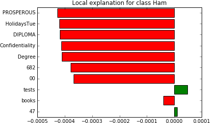
Figure 7-3 presents this data in chart form.

mlas 0703
Figure 7-3. Linear weighted features contributing to MNB prediction

Observe that the words “PROSPEROUS,” “HolidaysTue,” “DIPLOMA,” and so on contribute negatively to the sample being classified as ham. More specifically, removing the word “PROSPEROUS” from the sample would cause the multinomial Naive Bayes algorithm to classify this example as spam with 0.0427% less confidence. This explanation that LIME produces allows an end user to inspect the components that contribute to a decision that a machine learning algorithm makes. By approximating arbitrary machine learning models with a localized and linear substitute model (described by the linear weighted features as illustrated in Figure 7-3), LIME does not require any specific model family and can easily be applied to existing systems.

Performance

By nature, many security machine learning systems are in the direct line of traffic, where they are forced to make rapid-fire decisions or risk falling behind. Detecting an anomaly 15 minutes after the event is often too late. Systems that have real-time adaptability requirements must also meet a high bar for efficiently implementing continuous incremental retraining.

Production machine learning systems have much stricter performance requirements than experimental prototypes. In some cases, prediction latencies that exceed the millisecond range can cause the downfall of an entire system. Furthermore, systems tend to fail when bombarded with a high load unless they are designed to be fault-tolerant and highly scalable. Let’s look at some ways to achieve low latency and high scalability in machine learning systems.

Goal: Low Latency, High Scalability

Machine learning, especially on large datasets, is a computationally intensive task. Scikit-learn puts out respectable performance numbers by any measure, and contributors are constantly making performance improvements to the project. Nevertheless, this performance can still be insufficient for the demands of some applications. For security machine learning systems in critical decision paths, the end user’s tolerance for high-latency responses might be limited. In such cases, it is often a good design choice to take machine learning systems out of the main line of interaction between users and a system.

Your security system should make its decisions asynchronously wherever possible, and it should be able to remediate or mitigate threats in a separate and independent path. For example, a web application intrusion detection system (IDS) implemented using machine learning can be continuously queried with incoming requests. This IDS must make real-time decisions as to whether a request is a threat. The web application can choose to let the request pass if it does not receive a reply from the IDS within a certain time threshold, so as not to the degrade user experience with unbearable wait times when the system is overloaded. When the IDS eventually returns a result and indicates that that previously passed request was a suspicious entity, it can trigger a hook within the web application to inform it of this decision. The web application can then choose to perform a variety of mitigating actions, such as immediately disallowing further requests made by the user.

However, such a system design might be unsuitable in some cases. For instance, if a single malicious request can cause a significant data breach, the attacker’s objectives might have already been met by the time the IDS decision is made. Attackers can even bombard the system with dummy requests to cause a slowdown in the IDS and increase the attack window. In such cases it is worthwhile to invest resources to optimizing the machine learning system to minimize latency, especially when under heavy load. (This scenario can arguably also be solved with tweaks to system design—single requests should not be allowed to cause a significant data breach or seriously damage a system.)

Performance Optimization

To speed up machine learning applications, we can search for performance bottlenecks in the program execution framework, find more efficient algorithms, or use parallelism. Let’s consider these different approaches:15

Profiling and framework optimization

Software profiling is a method of dynamically analyzing the performance of a program. We do this instrumenting of the software with a tool called a profiler. The profiler typically inserts hooks into components, functions, events, code, or instructions being executed, and does a deep analysis of the time it takes for each individual component to run. The data collected allows the operator to gain deep insight into the internal performance characteristics of the software and identify performance bottlenecks. Profiling is a well-known and general part of the software developer’s toolkit, and should be actively used by machine learning engineers working on optimizing algorithms or systems for production.

Core algorithms in scikit-learn are frequently Cython wrappers around other popular and well-maintained machine learning libraries written in native C or C++ code. For example, the SVM classes in scikit-learn mostly hook into LIBSVM,16 which is written in C++. Furthermore, matrix multiplication (which is a very common operation in machine learning algorithms) and other vector computations are usually handled by NumPy, which uses native code and machine-level optimizations to speed up operations.17 Nevertheless, there are always performance bottlenecks, and performance profiling is a good way to find them if performance is a problem in your machine learning application. The IPython integrated profiler is a good place to start. When dealing with large datasets and memory-intensive models, the program might be memory bound rather than compute bound. In such cases, a tool like memory_profiler can help to find certain lines or operations that are memory hogs so that you can remedy the problem.

There is an endless list of framework-level performance optimizations that you can apply to machine learning applications that we will not go into here. Such optimizations will commonly help algorithms achieve speed increases of two to five times, but it is rare for major improvements to result from these.

Algorithmic optimization

Algorithmic improvements and picking efficient models can often bring greater performance improvements. Losing some accuracy for a huge performance improvement can be a worthwhile trade-off, depending on the context. Because model selection is such a context- and application-specific process, there is no hard-and-fast ruleset for how to achieve better performance and scalability by choosing certain algorithms over others. Nonetheless, here is a teaser list of tips that might be useful in your decision-making process:

  • Having fewer features means having to do fewer arithmetic operations, which can improve performance. Applying dimensionality reduction methods to remove useless features from your dataset can improve performance.

  • Tree-based models (e.g., decision trees, random forests) tend to have very good prediction performance because every query interacts only with a small portion of the model space (one root-to-leaf path per tree). Depending on architecture and hyperparameter choices, neural network predictions can sometimes be speedier than random forests.18

  • Linear models are fast to train and evaluate. Training of linear models can be parallelized with a popular algorithm called the Alternating Direction Method of Multipliers (ADMM),19 which allows the training of large linear models to scale very well.

  • SVMs suffer from widely known scalability problems. They are one of the slower model families to train and are also very memory intensive. Simple linear SVMs are usually the only choice for deploying on large datasets. However, evaluations can be quite fast if kernel projections are not too complex. It is possible (but complicated) to parallelize SVM training.20

  • Deep learning algorithms (deep neural nets) are slow to train and quite resource intensive (typically at least millions of matrix multiplications involved), but can easily be parallelized with the appropriate hardware—e.g., graphics processing units (GPUs)—and modern frameworks such as TensorFlow, Torch, or Caffe.

  • Approximate nearest neighbor search algorithms such as k-d trees (which we introduced in Chapter 2) can significantly speed up close-proximity searches in large datasets. In addition, they are generally very fast to train and have very fast average performance with bounded error. Locality sensitive hashing (LSH, which we used in Chapter 1) is another approximate nearest neighbor search method.

Horizontal Scaling with Distributed Computing Frameworks

Parallelization is a key tenet of performance optimization. By distributing a collection of 100 independent compute operations to 100 servers, we can achieve a speedup in processing time of up to 100 times (ignoring I/O and shuffling latency). Many steps of the machine learning process can benefit from parallelism, but many datasets and algorithms cannot be “blindly distributed” because each unit of operation might not be independent. For instance, the training of a random forest classifier is embarrassingly parallel because each randomized decision tree that makes up the forest is independently created and can be individually queried for the generation of the final prediction. However, other algorithms (e.g., SVMs) are not so straightforward to parallelize, because they require frequent global message passing (between nodes) during the training and/or prediction phase, which can sometimes incur an exponentially increasing cost as the degree of distribution increases. We do not go into the theory of parallel machine learning here; instead, let’s look at how to take advantage of frameworks to horizontally scale our machine learning systems in the quickest ways possible.

Distributed machine learning is not just about training classification or clustering algorithms on multiple machines. Scikit-learn is designed for single-node execution, but there are some types of tasks that are better suited for the distributed computing paradigm. For instance, hyperparameter optimization and model search operations (discussed in “Problem: Hyperparameter Optimization”) create a large number of symmetrical tasks with no mutual dependency. These types of embarrassingly parallel tasks are well suited for distributed MapReduce21 frameworks such as Apache Spark. Spark is an open source distributed computing platform that heavily uses memory-based architectures, lazy evaluation, and computation graph optimization to enable high-performance MapReduce-style programs.

spark-sklearn is a Python package that integrates the Spark computing framework with scikit-learn, focused on hyperparameter optimization. Even though there is (as of this writing) quite a limited set of scikit-learn’s functionality implemented in spark-sklearn, the classes that do exist are drop-in replacements into existing scikit-learn applications. Let’s see how the spark_sklearn.GridSearchCV22 class can help with our digit classification Support Vector Classifier hyperparameter search operation from the section “Solutions: Hyperparameter Optimization”:

from sklearn.svm import SVC
import numpy as np
from time import time
from spark_sklearn import GridSearchCV # This is the only changed line

# Define a dictionary containing all hyperparameter values to try
hyperparam_grid = {
    'kernel': ['linear', 'poly', 'rbf', 'sigmoid'],
    'gamma': np.linspace(0.001, 0.01, num=10),
    'C': np.linspace(1, 10, num=10),
    'tol': np.linspace(0.001, 0.01, 10)
}

classifier = GridSearchCV(svc, hyperparam_grid)

start = time()
classifier.fit(X_train, y_train)
elapsed = time()  start
...
print('elapsed: %.2f seconds' % elapsed)

> elapsed: 1759.71 seconds
> Best Kernel: rbf
> Best Gamma: 0.001
> Best C: 2.0
> Accuracy: 0.991

The hyperparam_grid passed into GridSearchCV specifies values for four hyperparameters that the optimization algorithm needs to consider. In total, there are 4,000 unique value combinations, which take 1,759.71 seconds to complete on a single eight-core23 machine using scikit-learn’s GridSearchCV. If we use the spark-sklearn library’s GridSearchCV instead (as in the preceding code snippet), and run the program on a five-node Spark cluster (one master, four workers, all the same machine type as in the single-machine example), we see an almost linear speedup—the tasks are executed only on the four-worker nodes:

> elapsed: 470.05 seconds

Even though spark-sklearn is very convenient to use and allows you to parallelize hyperparameter optimization across a cluster of machines with minimal development effort, its feature set is quite small.24 Furthermore, it is intended for datasets that fit in memory, which limits its usefulness. For more heavyweight production applications, Spark ML offers a respectable set of parallelized algorithms that have been implemented and optimized to run as MapReduce-style jobs on distributed Spark clusters. As one of the most mature and popular distributed machine learning frameworks, Spark ML goes beyond providing common machine learning algorithms for classification and clustering: it also provides for distributed feature extraction and transformation, allows you to create pipelines for flexible and maintainable processing, and lets you save serialized versions of machine learning objects for checkpointing and migration.

Let’s try using some of the Spark ML APIs on the same spam classification dataset that we used in Chapter 1 as well as earlier in this chapter, in “Generating explanations with LIME”. In particular, we will focus on using Spark ML pipelines to streamline our development workflow. Similar to scikit-learn pipelines, Spark ML pipelines allow you to combine multiple sequential operations into a single logical stream, facilitated by a unified API interface. Pipelines operate on Spark DataFrames, which are optimized columnar-oriented datasets, similar to Pandas DataFrames but supporting Spark transformations. We implement a spam classification pipeline using Spark ML, omitting the email parsing and dataset formatting code because we can reuse the same code as before:25

from pyspark.sql.types import *
from pyspark.ml import Pipeline
from pyspark.ml.feature import Tokenizer, CountVectorizer
from pyspark.ml.classification import RandomForestClassifier
from pyspark.ml.evaluation import BinaryClassificationEvaluator

# Read in the raw data
X, y = read_email_files()

# Define a DataFrame schema to specify the names and
# types of each column in the DataFrame object we will create
schema = StructType([
            StructField('id', IntegerType(), nullable=False),
            StructField('email', StringType(), nullable=False),
            StructField('label', DoubleType(), nullable=False)])

# Create a Spark DataFrame representation of the data with
# three columns, the index, email text, and numerical label
df = spark.createDataFrame(zip(range(len(y)), X, y), schema)

# Inspect the schema to ensure that everything went well
df.printSchema()

> root
  |-- id: integer (nullable = false)
  |-- email: string (nullable = false)
  |-- label: double (nullable = false)

A small quirk of Spark ML is that it requires labels to be of the Double type. (If you fail to specify this, you will run into errors when executing the pipeline.) We created a StructType list in the preceding example, which we passed as the schema into the spark.createDataFrame() function for converting the Python list-type dataset to a Spark DataFrame object. Now that we have our data in a Spark-friendly format, we can define our pipeline (almost all Spark ML classes support the explainParams() or explainParam(paramName) function, which conveniently prints out the relevant documentation snippets to give you a description of the parameters for this class—a very useful feature, especially given that Spark ML documentation is sometimes difficult to locate):

# Randomly split the dataset up into training and test sets, where
# TRAINING_SET_RATIO=0.7 (seed set for reproducibility)
train, test = df.randomSplit([TRAINING_SET_RATIO, 1-TRAINING_SET_RATIO], seed=123)

# First, tokenize the email string (convert to
# lowercase then split by whitespace)
tokenizer = Tokenizer()

# Second, convert the tokens into count vectors
vectorizer = CountVectorizer()

# Third, apply the RandomForestClassifier estimator
rfc = RandomForestClassifier()

# Finally, create the pipeline
pipeline = Pipeline(stages=[tokenizer, vectorizer, rfc])

A convenient feature of ML pipelines is the ability to specify parameters for pipeline components in a parameter dictionary that can be passed into the pipeline upon execution. This allows for neat separation of application logic and tunable parameters, which might seem like a small feature but can make a lot of difference in the maintainability of code. Notice that we didn’t specify any parameters when initializing the pipeline components (Tokenizer, CountVectorizer, RandomForestClassifier) in the previous example—if we had specified any, they would just have been overwritten by parameters passed in the call to the pipeline.fit() function, which executes the pipeline:

# Define a dictionary for specifying pipeline component parameters
paramMap = {
    tokenizer.inputCol: 'email',
    tokenizer.outputCol: 'tokens',

    vectorizer.inputCol: 'tokens',
    vectorizer.outputCol: 'vectors',

    rfc.featuresCol: 'vectors',
    rfc.labelCol: 'label',
    rfc.numTrees: 500
}

# Apply all parameters to the pipeline,
# execute the pipeline, and fit a model
model = pipeline.fit(train, params=paramMap)

We now have a trained pipeline model that we can use to make predictions. Let’s run a batch prediction on our test set and evaluate it using the BinaryClassificationEvaluator object, which automates all of the data wrangling necessary for generating evaluation metrics:

# Make predictions on the test set
prediction = model.transform(test)

# Evaluate results using a convenient Evaluator object
evaluator = BinaryClassificationEvaluator(rawPredictionCol='rawPrediction')
pr_score = evaluator.evaluate(prediction,
{evaluator.metricName: 'areaUnderPR'})
roc_score = evaluator.evaluate(prediction,
{evaluator.metricName: 'areaUnderROC'})

print('Area under ROC curve score: {:.3f}'.format(roc_score))
print('Area under precision/recall curve score: {:.3f}'.format(pr_score))

> Area under ROC curve score: 0.971
> Area under precision/recall curve score: 0.958

With the help of Spark ML, we have written a concise yet highly scalable piece of code that can handle a punishing load of data.26 Spark ML pipelines help create elegant code structure, which can be very helpful as your code base grows. You can also add hyperparameter optimization logic to the pipeline by configuring a ParamGridBuilder object (for specifying hyperparameter candidates) and a CrossValidator or TrainValidationSplit object (for evaluating hyperparameter/estimator efficacy).27

Spark provides convenient ways to use parallelization and cluster computing to achieve lower latencies and higher scalability in machine learning systems. Distributed programming can be significantly more complicated than local development in scikit-learn, but the investment in effort will pay dividends over time.

Using Cloud Services

The machine-learning-as-a-service market is predicted to grow to $20 billion by 2025. All of the popular public cloud providers have several machine learning and data infrastructure offerings that you can use to quickly and economically scale your operations. These services relieve organizations of the operational overhead of managing a Spark cluster or TensorFlow deployment that requires significant effort to configure and maintain.

The largest players in the public cloud arena, such as Amazon Web Services (AWS) and Google Cloud Platform (GCP), provide powerful APIs for video, speech, and image analysis using pretrained machine learning models. They also provide serverless interfaces to run experimental or production machine learning jobs, without ever having to link via Secure Shell (SSH) into an instance to install dependencies or reboot processes. For example, Google Cloud Dataflow is a fully managed platform that allows users to execute jobs written in the Apache Beam unified programming model, without having to fret over load and performance. Scaling up to 10 times the throughput will simply be a matter of changing a parameter to launch approximately 10 times more instances to deal with the load. Google Cloud Dataproc is a managed Spark and Hadoop service that allows you to spin up large clusters of machines (preloaded and preconfigured with Spark, Hadoop, Pig, Hive, Yarn, and other distributed computing tools) in “less than 90 seconds on average.” For instance, setting up a five-node Spark cluster on Dataproc for running the Spark ML spam classification example from earlier in this section took less than a minute after running this gcloud command on the command line:

gcloud dataproc clusters create cluster-01 \
    --metadata "JUPYTER_CONDA_PACKAGES=numpy:pandas:scipy:scikit-learn" \
    --initialization-actions \
        gs://dataproc-initialization-actions/jupyter/jupyter.sh \
    --zone us-central1-a \
    --num-workers 4 \
    --worker-machine-type=n1-standard-8 \
    --master-machine-type=n1-standard-8

The cluster creation command allows users to specify initialization-actions—a script for installing custom packages and data/code dependencies that will be executed during the provisioning phase of each machine in the cluster. In the preceding command, we used an initialization-actions script to install a Jupyter notebook and the Python package dependencies Pandas, SciPy, and so on.

Amazon Machine Learning allows even novices to take advantage of machine learning by uploading data to their platforms (e.g., S3 or Redshift) and “creating” a machine learning model by tweaking some preference settings on a web interface. Google Cloud ML Engine allows for much more flexibility, giving users the ability to run custom TensorFlow model training code on a serverless architecture, and then save the trained model and expose it through a predictions API. This infrastructure makes it possible for machine learning engineers to focus solely on the efficacy of their algorithms and outsource operational aspects of deploying and scaling a machine learning system.

Using cloud services can give organizations a lot of flexibility in experimenting with machine learning solutions. These solutions will often even be more cost effective after you consider all of the operational and maintenance costs that go into manually managing machine learning deployments. For organizations that must deal with variation in machine learning system implementation and architectures, or operate systems that will potentially need to scale significantly over a short period of time, using public cloud offerings such as Google Cloud ML Engine makes a lot of sense. However, the availability of such services is entirely dependent on their parent organization’s business needs (i.e., how profitable it is to Amazon, Google, Microsoft, etc.), and building critical security services on top of them might not be a sound strategic decision for everyone.

Maintainability

Successful machine learning systems in production often outlive their creators (within an organization). As such, these systems must be maintained by engineers who don’t necessarily understand why certain development choices were made. Maintainability is a software principle that extends beyond security and machine learning. All software systems should optimize for maintainability, because poorly maintained systems will eventually be deprecated and killed. Even worse, such systems can limp along for decades, draining resources from the organization and preventing it from implementing its goals. A recent paper from Google28 argues that due to their complexity and dependence on ever-changing data, machine learning systems are even more susceptible than other systems to buildup of technical debt.

In this section we briefly touch on a few maintainability concepts. We do not go into great detail, because many of these concepts are covered in depth in dedicated publications.29

Problem: Checkpointing, Versioning, and Deploying Models

Is a machine learning model code or data? Because models are so tightly coupled to the nature of the data used to generate them, there is an argument that they should be treated as data, because code should be independent of the data it processes. However, there is operational value in subjecting models to the same versioning and deployment processes that conventional source code is put through. Our view is that machine learning models should be treated both as code and data. Storing model parameters/hyperparameters in version-control systems such as Git makes the restoration of previous models very convenient when something goes wrong. Storing models in databases allows for querying parameters across versions in parallel, which can be valuable in some contexts.

For audit and development purposes, it is good to ensure that any decision that a system makes at any point in time can be reproduced. For instance, consider a web application anomaly detection server that flags a particular user session as anomalous. Because of the high fluctuations in input that web applications can see, this system attempts to continuously measure and adapt to the changing traffic through continuous and automatic parameter tuning. Furthermore, machine learning models are continuously tuned and improved over time, whether due to automated learning mechanisms or human engineers. Checkpointing and versioning of models enables us to see if this user session would have triggered the model from two months ago.

Serializing models for storage can be as simple as using the Python pickle object serialization interface. For space and performance efficiency as well as better portability, you can use a custom storage format that saves all parameter information required to reconstruct a machine learning model. For instance, storing all the feature weights of a trained linear regression model in a JSON file is a platform- and framework-agnostic way to save and reconstruct linear regressors.

Predictive Model Markup Language (PMML) is the leading open standard for XML-based serialization and sharing of predictive data mining models.30 Besides storing model parameters, the format can also encode various transformations applied to the data in preprocessing and postprocessing steps. A convenient feature of the PMML format is the ability to develop a model using one machine learning framework and deploy it on a different machine learning framework. As the common denominator between different systems, PMML enables developers to compare the performance and accuracy of the same model executed on different machine learning frameworks.

The deployment mechanism for machine learning models should be engineered to be as foolproof as possible. Machine learning systems can be deployed as web services (accessible via REST APIs, for example), or embedded in backend software. Tight coupling with other systems is discouraged because it causes a lot of friction during deployment and results in a very inflexible framework. Accessing machine learning systems through APIs adds a valuable layer of indirection which can lend a lot of flexibility during the deployment, A/B testing, and debugging process.

Goal: Graceful Degradation

Software systems should fail gracefully and transparently. If a more advanced and demanding version of a website does not work on an old browser, a simpler, lightweight version of the site should be served instead. Machine learning systems are no different. Graceful failure is an important feature for critical systems that have the potential to bring down the availability of other systems. Security systems are frequently in the critical path, and there has to be a well-defined policy for how to deal with failure scenarios.

Should security systems fail open (allow requests through if the system fails to respond) or fail closed (block all requests if the system fails to respond)? This question cannot be answered without a comprehensive study of the application, weighing the risk and cost of an attack versus the cost of denying real users access to an application. For example, an authentication system will probably fail closed, because failing open would allow anybody to access the resources in question; an email spam detection system, on the other hand, will fail open, because blocking everyone’s email is much more costly than letting some spam through. In the general case, the cost of a breach vastly outweighs the cost of users being denied service, so security systems typically favor policies that define a fail-closed strategy. In some scenarios, however, this will make the system vulnerable to denial-of-service attacks, since attackers simply have to take down the security gateway to deny legitimate users access to the entire system.

Graceful degradation of security systems can also be achieved by having simpler backup systems in place. For instance, consider the case in which your website is experiencing heavy traffic volumes and your machine learning system that differentiates real human traffic from bot traffic is at risk of buckling under the stress. It may be wise to fall back to a more primitive and less resource-intensive strategy of CAPTCHAs until traffic returns to normal.

A well-thought-out strategy for ensuring continued system protection when security solutions fail is important because any loopholes in your security posture (e.g., decreased system availability) represent opportunities for attackers to get in.

Goal: Easily Tunable and Configurable

Religious separation of code and configuration is a basic requirement for all production-quality software. This principle holds especially true for security machine learning systems. In the world of security operations, configurations to security systems often have to be tuned by security operations analysts, who don’t necessarily have a background in software development. Designing software and configuration that empowers such analysts to tune systems without the involvement of software engineers can significantly reduce the operational costs of such systems and make for a more versatile and flexible organization.

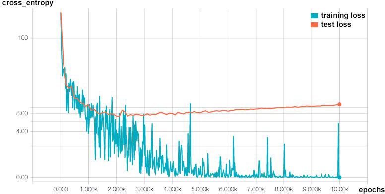
Monitoring and Alerting

Security machine learning systems should be fast and robust. Ideally, such systems should never see any downtime and predictions should be made in near real time.31 However, the occasional mishap that results in a performance slowdown or system outage is inevitable. Being able to detect such events in a timely fashion allows for mitigations that can limit their detrimental effects, for example by having backup systems kick in and operational personnel called to investigate the issue.

A monitoring framework is a system that aggregates metrics from different sources in a central place for manual monitoring and performing anomaly detection. Such systems are often made up of five distinct components:

  • Metrics collectors

  • Time series database

  • Detection engine

  • Visualization layer

  • Alerting mechanism

A typical workflow for application monitoring starts when applications periodically publish metrics to a monitoring framework collection point (e.g., a REST endpoint), or when metric collector agents on the endpoints extract metrics from the system. These metrics are then stored in the time series database, which the detection engine can query to trigger alerts and the visualization layer can use to generate charts. The alerting mechanism is then in charge of informing relevant stakeholders of notable occurrences automatically detected by the framework.

Monitoring and alerting frameworks are often in the predicament of being able to alert administrators when other systems go down but not being able to do so when they experience downtime themselves. Although it is impossible to completely remove this risk, it is important to design or select monitoring systems that are themselves highly available, robust, and scalable. Adding redundancy in monitoring solutions can also decrease the probability of a total loss of visibility when a single machine goes down. An involved discussion of monitoring is beyond the scope of this book, but it is worthwhile to invest time and effort to learn more about effective monitoring and alerting.32 Popular monitoring frameworks such as Prometheus, the TICK stack, Graphite, and Grafana are good candidates for getting started.

Performance and availability are not the only system properties that should be monitored. Because these statistical systems consume real-world data that is subject to a certain degree of unpredictability, it is also important to monitor the general efficacy of the system to ensure that relevant and effective results are consistently produced. This task is seldom straightforward since measures of efficacy necessarily require having access to some way to reliably check if predictions are correct, and often involve human labels from feedback loops. A common approximation for measuring changes in efficacy is to monitor the distribution of system predictions served. For instance, if a system that typically sees 0.1% of login requests marked as suspicious sees this number suddenly jump to 5%, it’s probably worth looking into.33

Another powerful feature is being able to monitor changes in the input data, independent of the machine learning system’s output. Data properties such as the statistical distribution, volume, velocity, and sparseness can have a large effect on the efficacy and performance of machine learning systems. Changes in data distributions over time could be an effect of shifting trends, acquiring new sources of data (e.g., a new customer or application feeding data to the system), or in rare cases adversarial poisoning (red herring attacks, which we discuss in Chapter 8). Increasing sparseness in incoming data is also a common occurrence that has negative effects on machine learning systems.

Data collection and feature extraction pipelines become stale when they don’t keep up with changing data formats. For instance, a web application feature extractor collecting IP addresses from HTTP requests may assume that all IP addresses are in the IPv4 format. When the website starts supporting IPv6, this assumption is then broken and we will observe a higher number of data points with a null IP field. Although it can be difficult to keep up with changing input data formats, monitoring the occurrence of missing fields in extracted feature sets makes for a good proxy. A changing trend in error or exception counts in individual system components (such as in the feature extraction pipeline) can also be a good early indicator of system failure; these counts should be a standard metric monitored in mature production systems.

Security and Reliability

Wherever security solutions are deployed, malicious activity should be expected. Let’s look at the security and privacy guarantees that security machine learning systems should provide.

Feature: Robustness in Adversarial Contexts

Security systems face a constant risk of adversarial impact. Attackers have constant motivation to circumvent protective walls put in place because there is, by nature, a likely payout on the other side. It is hence necessary for production systems to be robust in the face of malicious activity attempting to bring down the performance, availability, or efficacy of such systems.

It is important to stress the confounding effects that active adversaries can have in influencing machine learning models. There is a significant body of research in this area, showing how much adversaries can do with minimal access and information. For security machine learning systems in particular, it is important to preempt attacker logic and capabilities. You should thus take care to select robust algorithms as well as design systems with the proper checks and balances in place that allow for tampering attempts to be detected and their effects limited.

A variety of different statistical attacks can be waged on machine learning systems, causing them to lose stability and reliability. As designers and implementers of security machine learning systems, we are in a unique position to protect these systems from adversarial impact. We will dive into a more detailed discussion of adversarial machine learning in Chapter 8, but it is important to consider whether the security machine learning systems that you put into production are susceptible to such attacks or not.

Feature: Data Privacy Safeguards and Guarantees

Data privacy is an increasingly relevant area of concern as technology becomes more pervasive and invasive. Machine learning systems are usually at odds with privacy protection because algorithms work well with more descriptive data. For instance, being able to access rich audio and camera captures from mobile devices can give us a lot of raw material for classifying the legitimacy of mobile app API requests made to an account login endpoint, but such broad access is typically considered to be a huge privacy violation and hence is seldom done in practice.

In addition to the privacy issues related to the collection of intrusive data from users and endpoints, there is also the issue of information leakage from trained machine learning models themselves.34 Some machine learning models generate outputs that allow an external observer to easily infer or reconstruct either the training data that went into model training or the test data that generated that prediction output. For instance, the k-NN algorithm and kernel-based support vector machines are particularly susceptible to information leakage because some training data can be inferred from density calculations and functions that represent the support vectors.35

The problem of building privacy-preserving machine learning algorithms has spawned an active field of research, and is difficult to solve because attackers often have access to global information. If an attacker has access to a trained machine learning model and to 50% or more of the training data, it will be possible for them to make high-confidence guesses about the makeup of the other 50%. Differential privacy36 refers to a class of privacy-preserving machine learning solutions that aims to solve this problem by making it more difficult for an attacker to make high-confidence guesses about a piece of missing information from his or her point of view.

Privacy in machine learning systems should be a top requirement because privacy violations and breaches usually have serious and expensive consequences. Production systems should be able to provide privacy safeguards and guarantees that are based on sound theoretical and technical frameworks and limit the harm that attackers can do to steal private information.

Feedback and Usability

User experiences that emphasize communication and collaboration between humans and machines while balancing machine automation and (the perception of) user agency are the true hallmarks of an outstanding security machine learning system. There is an inherent distrust between humans and machines. Machine learning solutions will not reach their full potential unless the user experience of such systems progresses along with them. Explainability of results is an important prerequisite for trust because most users will not trust the results of systems if they don’t understand how the system arrived at the result. Transparency is key to fully exploiting the power that machine learning systems can provide. If a fraudulent login detection system uses machine learning to determine that a particular login attempt is suspicious, the system should attempt to inform the user of the reasons behind this decision and what they can do to remedy the situation.

Of course, full explainability is at odds with security principles, which dictate that systems should reveal as little as possible to potential attackers. Giving attackers a feedback channel allows them to iterate quickly and develop exploits that will eventually be able to fool systems. A potential solution is to scale the transparency of a machine learning engine’s decisions inversely with how likely it is to be engaging with an attacker. If the system is able to classify typical attack behavior with high confidence, and most false positives are not “high-confidence positives,” it can implement a discriminating transparency policy that keeps obvious attackers from getting any feedback. This setup allows for some flexibility in mitigating the negative effects of wrong predictions made by machine learning systems.

The presentation of information in the human-machine interface of machine learning systems is an area of study that is often neglected. Poor management of the bias, trust, and power dynamics between humans and security machine learning systems can cause their downfall.

Conclusion

Security machine learning systems must be one of the strongest links in a modern application environment. As such, these systems need to meet quality, scalability, and maintainability standards that surpass most other components in an operation. In this chapter, we provided a framework for evaluating a system’s production readiness; it is now your job, as security data scientists and engineers, to ensure that the software you deploy is truly production ready.

1 Note that bias (or algorithmic bias) in statistics and machine learning is also a term used to describe errors in assumptions made by a learning algorithm that can cause algorithms to underfit. Our use of the term here is different; we refer to data bias here, which refers to a dataset’s inadequate representation of a population.

2 Clickjacking is a web attack technique that tricks users into clicking something different from what they perceive they are clicking, usually by presenting a false interface on top of the original one. Clickjacking makes users do something unintended that benefits the attacker, such as revealing private information, granting access to some resource, or taking a malicious action.

3 J.L. Fleiss and J. Cohen, “The Equivalence of Weighted Kappa and the Intraclass Correlation Coefficient as Measures of Reliability,” Educational and Psychological Measurement 33 (1973): 613–619.

4 Full code can be found as a Python Jupyter notebook, chapter7/missing-values-imputer.ipynb in our code repository.

5 Most implementations of k-NN algorithms don’t actually store the entire training dataset as the model. For prediction-time efficiency, k-NN implementations commonly make use of data structures such as k-d trees. See J.L. Bentley, “Multidimensional Binary Search Trees Used for Associative Searching,” Communications of the ACM 18:9 (1975): 509.

6 A.M. Kibriya and E. Frank, “An Empirical Comparison of Exact Nearest Neighbour Algorithms,” Proceedings of the 11th European Conference on Principles and Practice of Knowledge Discovery in Databases (2007): 140–151.

7 Yann LeCun, Corinna Cortes, and Christopher Burges, “The MNIST Database of Handwritten Digits” (1998).

8 Nitish Srivastava et al., “Dropout: A Simple Way to Prevent Neural Networks from Overfitting,” Journal of Machine Learning Research 15 (2014): 1929–1958.

9 Burr Settles, “Active Learning Literature Survey,” Computer Sciences Technical Report 1648, University of Wisconsin–Madison (2010).

10 Tyler Lu, Dávid Pál, and Martin, Pál, “Contextual Multi-Armed Bandits,” Journal of Machine Learning Research Proceedings Track 9 (2010): 485–492.

11 Marco Tulio Ribeiro, Sameer Singh, and Carlos Guestrin, "Why Should I Trust You?: Explaining the Predictions of Any Classifier,” Proceedings of the 22nd ACM SIGKDD International Conference on Knowledge Discovery and Data Mining (2016): 1135–1144.

12 Ryan Turner, “A Model Explanation System,” Black Box Learning and Inference NIPS Workshop (2015).

13 Ryan Turner, “A Model Explanation System: Latest Updates and Extensions,” Proceedings of the 2016 ICML Workshop on Human Interpretability in Machine Learning (2016): 1–5.

14 Full code is provided as a Python Jupyter notebook chapter7/lime-explainability-spam-fighting.ipynb in our code repository.

15 Parallelism as a method for performance optimization is elaborated on further in “Horizontal Scaling with Distributed Computing Frameworks”.

16 Chih-Chung Chang and Chih-Jen Lin, “LIBSVM: A Library for Support Vector Machines,” Transactions on Intelligent Systems and Technology 2:3 (2011).

17 See the recipe “Getting the Best Performance out of NumPy” from Cyrille Rossant’s IPython Interactive Computing and Visualization Cookbook (Packt).

18 This observation comes with hefty caveats: for instance, model size, GPU versus CPU, and so on.

19 Stephen Boyd et al., “Distributed Optimization and Statistical Learning via the Alternating Direction Method of Multipliers,” Foundations and Trends in Machine Learning 3 (2011): 1–122.

20 Edward Y. Chang et al., “PSVM: Parallelizing Support Vector Machines on Distributed Computers,” Proceedings of the 20th International Conference on Neural Information Processing Systems (2007) 257–264.

21 Jeffrey Dean and Sanjay Ghemawat, “MapReduce: Simplified Data Processing on Large Clusters,” Proceedings of the 6th Symposium on Operating Systems Design and Implementation(2004): 137–150.

22 This example uses version 0.2.0 of the spark-sklearn library.

23 Eight Intel Broadwell CPUs, 30 GB memory.

24 Note that spark-sklearn does not implement individual learning algorithms such as SVMs or k-means. It currently implements only simple and easily parallelized tasks like grid search cross-validation.

25 Full code can be found as a Python Jupyter notebook at chapter7/spark-mllib-spam-fighting.ipynb in our code repository.

26 This example was run on a five-node Spark cluster (one master, four workers) on Google’s DataProc engine.

27 For details on all of these, see the documentation.

28 D. Sculley et al., “Hidden Technical Debt in Machine Learning Systems,” Proceedings of the 28th International Conference on Neural Information Processing Systems (2015): 2503–2511.

29 Joost Visser et al., Building Maintainable Software, Java Edition: Ten Guidelines for Future-Proof Code (Sebastopol, CA: O’Reilly Media, 2016).

30 Alex Guazzelli et al., “PMML: An Open Standard for Sharing Models,” The R Journal 1 (2009): 60–65.

31 “Architecting a Machine Learning System for Risk”, by Naseem Hakim and Aaron Keys, provides an insightful view into how a large company like Airbnb designs real-time security machine learning and risk-scoring frameworks.

32 Slawek Ligus, Effective Monitoring and Alerting for Web Operations (Sebastopol, CA: O’Reilly Media, 2012).

33 A big jump or an anomaly of this sort means something has changed either in the data or in the system. This could be due to an attack on the login endpoint of your site, or could be due to subtler issues like an incorrectly trained or tuned model that is causing a much higher rate of false positives than before.

34 Daniel Hsu, “Machine Learning and Privacy”, Columbia University, Department of Computer Science.

35 Zhanglong Ji, Zachary C. Lipton, and Charles Elkan, “Differential Privacy and Machine Learning: A Survey and Review” (2014).

36 Cynthia Dwork and Aaron Roth, “The Algorithmic Foundations of Differential Privacy,” Foundations and Trends in Theoretical Computer Science 9 (2014): 211–407.