Table of Contents for
Machine Learning and Security
 Machine Learning and Security
Published by
O'Reilly Media, Inc., 2018
Machine Learning and Security
Published by
O'Reilly Media, Inc., 2018
- nav
- Cover
- Praise for Machine Learning and Security
- Machine Learning and Security
- Machine Learning and Security
- Preface
- 1. Why Machine Learning and Security?
- 2. Classifying and Clustering
- 3. Anomaly Detection
- 4. Malware Analysis
- 5. Network Traffic Analysis
- 6. Protecting the Consumer Web
- 7. Production Systems
- 8. Adversarial Machine Learning
- A. Supplemental Material for Chapter 2
- B. Integrating Open Source Intelligence
- Index
- About the Authors
- Colophon
Chapter 5. Network Traffic Analysis
The most likely way that attackers will gain entry to your infrastructure is through the network. Network security is the broad practice of protecting computer networks and network-accessible endpoints from malice, misuse, and denial.1 Firewalls are perhaps the best-known network defense systems, enforcing access policies and filtering unauthorized traffic between artifacts in the network. However, network defense is about more than just firewalls.
In this chapter, we look at techniques for classifying network traffic. We begin by building a model of network defense upon which we will base our discussions. Then, we dive into selected verticals within network security that have benefited from developments in artificial intelligence and machine learning. In the second part of this chapter, we work through an example of using machine learning to find patterns and discover correlations in network data. Using data science as an investigation tool, we discover how to apply classification on complex datasets to uncover attackers within the network.
Our discussion of network security is limited to packet-based information transmission. In packet-based transmission, a data stream is segmented into smaller units, each of which contains some metadata about the transmission origin, destination, and content. Each packet is transmitted over the network layer and formatted in an appropriate protocol by the transport layer, with the reconstruction of the information stream from individual packets occurring at the session layer or above. The security of the network, transport, and session layers (layers 3, 4, and 5 of the OSI model, respectively) are the focus of this chapter.
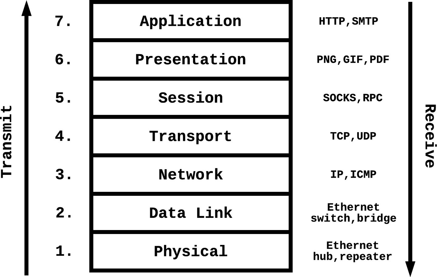
Figure 5-1. OSI seven-layer networking stack
As discussed in earlier chapters, attackers target networks mostly as a means to achieving the larger goals of espionage, data exfiltration, mischief, and more. Because of the complexity and ubiquity of connectivity between computer systems, attackers can frequently find ways to gain access into even the most carefully designed systems. We therefore focus our study of network security on scenarios that assume that the attacker has already breached the perimeter and is actively attacking the network from within.
Theory of Network Defense
Networks have a complicated defense model because of the broad range of attack surfaces and threat vectors. As is the case when defending any complicated system, administrators need to engage with attackers on multiple fronts and must make no assumptions about the reliability of any one component of the solution.
Access Control and Authentication
A client’s interaction with a network begins with the access control layer. Access control is a form of authorization by which you can control which users, roles, or hosts in the organization can access each segment of the network. Firewalls are a means of access control, enforcing predefined policies for how hosts in the network are allowed to communicate with one another. The Linux kernel includes a built-in firewall, iptables, which enforces an IP-level ruleset that dictates the ingress and egress capabilities of a host, configurable on the command line. For instance, a system administrator who wants to configure iptables to allow only incoming Secure Shell (SSH) connections (over port 22) from a specific subnet, 192.168.100.0/24,2 might issue the following commands:
# ACCEPT inbound TCP connections from 192.168.100.0/24 to port 22
iptables --append INPUT --protocol tcp --source 192.168.100.0/24
         --dport 22 --jump ACCEPT

# DROP all other inbound TCP connections to port 22
iptables --append INPUT --protocol tcp --dport 22 --jump DROP
Just like locks on the doors of a building, access control policies are important to ensure that only end users who are granted access (a physical key to a locked door) can enter the network. However, just as a lock can be breached by thieves who steal the key or break a window, passive access control systems can be circumvented. An attacker who gains control of a server in the 192.169.100.0/24 subnet can access the server because this passive authentication method relies on only a single property—the connection’s origin—to grant or deny access.
Active authentication methods gather more information about the connecting client, often using cryptographic methods, private knowledge, or distributed mechanisms to achieve more reliable client identity attestation. For instance, in addition to using the connection origin as a signal, the system administrator might require an SSH key and/or authentication credentials to allow a connection request. In some cases, multifactor authentication (MFA) can be a suitable method for raising the bar for attackers wanting to break in. MFA breaks up the authentication into multiple parts, causing attackers to have to exploit multiple schemes or devices to get both parts of the key to gain the desired access.
Intrusion Detection
We discussed intrusion detection systems in detail in Chapter 3. Intrusion detection systems go beyond the initial access control barriers to detect attempted or successful breaches of a network by making passive observations. Intrusion prevention systems are marketed as an improvement to passive intrusion detection systems, having the ability to intercept the direct line of communication between the source and destination and automatically act on detected anomalies. Real-time packet sniffing is a requirement for any intrusion detection or prevention system; it provides both a layer of visibility for content flowing through a network’s perimeter and data on which threat detection can be carried out.
Detecting In-Network Attackers
Assuming that attackers can get past access control mechanisms and avoid detection by intrusion detection systems, they will have penetrated the network perimeter and be operating within the trusted bounds of your infrastructure. Well-designed systems should assume that this is always the case and work on detecting in-network attackers. Regardless of whether these attackers are intruders or corrupted insiders, system administrators need to aggressively instrument their infrastructure with monitors and logging to increase visibility within and between servers. Just protecting the perimeter is not sufficient, given that an attacker who spends enough time and resources on breaching the perimeter will often be successful.
Proper segmentation of a network can help limit the damage caused by in-network attackers. By separating public-facing systems from high-valued central information servers and allowing only closely guarded and monitored API access between separate network segments, administrators narrow the channels available for attackers to pivot, allowing greater visibility and the ability to audit traffic flowing between nodes. Microsegmentation is the practice of segmenting a network into various sections based on each element’s logical function. Proper microsegmentation can simplify the network and the management of security policies, but its continued effectiveness is contingent on having stringent infrastructure change processes. Changes in the network must be accurately reflected in the segmentation schemes, which can be challenging to manage as the complexity of systems increase. Nevertheless, network segmentation allows administrators an opportunity to enforce strict control on the number of possible paths between node A and node B on a network, and also provides added visibility to enable the use of data science to detect attackers.
Data-Centric Security
When the perimeter is compromised, any data stored within the network is at risk of being stolen. Attackers who gain access to a network segment containing user credentials have unfettered access to the information stored within, and the only way to limit the damage is to employ a data-centric view of security. Data-centric security emphasizes the security of the data itself, meaning that even if a database is breached, the data might not be of much value to an attacker. Encrypting stored data is a way to achieve data-centric security, and it has been a standard practice to salt and hash stored passwords—as implemented in Unix operating systems—so that attackers cannot easily make use of stolen credentials to take over user accounts. Nevertheless, encryption of stored data is not suitable for all contexts and environments. For datasets that are actively used in analysis and/or need to be frequently used in unencrypted form, continuously encrypting and decrypting the data can come with unrealistically high resource requirements.
Performing data analysis on encrypted data is a goal that the security and data mining research communities have been working toward for a long time, and is sometimes even seen as the holy grail of cryptography.3 Homomorphic encryption presents itself as the most promising technique that allows for this. You can use a fully homomorphic encryption scheme such as the Brakerski-Gentry-Vaikuntanathan (BGV) scheme4 to perform computation without first decrypting the data. This allows different data processing services that work on the same piece of data to pass an encrypted version of the data to each other potentially without ever having to decrypt the data. Even though homomorphic encryption schemes are not yet practical at large scale, improving their performance is an active area of research. HElib is an efficiently implemented library for performing homomorphic encryption using low-level functions and the BGV encryption scheme.
Honeypots
Honeypots are decoys intended for gathering information about attackers. There are many creative ways to set up honeypot servers or networks (also referred to as honeynets), but the general goals of these components are to learn about attack methodologies and goals as well as to gather forensic information for performing analysis on the attacker’s actions. Honeypots present interfaces that mimic the real systems, and can sometimes be very successful in tricking attackers into revealing characteristics of their attack that can help with offline data analysis or active countermeasures. Honeypots strategically placed in environments that experience a sizable volume of attacks can be useful for collecting labeled training data for research and improving attack detection models.
Summary
So far in this chapter, we have provided a 10,000-foot view of network security, selecting a few highlights appropriate for the context of using machine learning for security. There are entire fields of study dedicated solely to network security and defense methodologies. As such, it is impossible to comprehensively cover the complexities of this topic in just a few paragraphs. In the remainder of this chapter, we dive deep into more specific attacks and methods of extracting security intelligence from network data using data science and machine learning.
Machine Learning and Network Security
Pattern mining is one of the primary strengths of machine learning, and there are many inherent patterns to be discovered in network traffic data. At first glance, the data in network packet captures might seem sporadic and random, but most communication streams follow a strict network protocol. For instance, when inspecting network packet captures, we can observe the TCP three-way handshake occurring, as shown in Figure 5-2.

Figure 5-2. TCP three-way handshake (source: Wireshark screen capture)
After identifying the handshake that marks the start of a TCP connection, we can isolate the rest of the corresponding TCP session. Identifying TCP sessions is not a particularly complex task, but it drives home the point that network traffic is strictly governed by a set of protocols that result in structures and patterns in the data. We can also find malicious activity in networks by mining for patterns and drawing correlations in the data, especially for attacks that rely on volume and/or iteration such as network scanning and denial of service (DoS) attacks.
From Captures to Features
Capturing live network data is the primary way of recording network activity for online or offline analysis. Like a video surveillance camera at a traffic intersection, packet analyzers (also known as packet/network/protocol sniffers) intercept and log traffic in the network. These logs are useful not only for security investigations, but also for debugging, performance studies, and operational monitoring. When situated in the right places in networks,5 and with network switches and interfaces correctly configured, packet analyzers can be a valuable tool for generating detailed datasets that give you a complete picture of everything that is going on in the network. As you can imagine, this data can be overwhelming. In complex networking environments, even simple tasks like tracing a TCP session, as we just did, will not be easy. With access to information-rich raw data, the next step will be to generate useful features for data analysis.
Let’s now look at some specific methods to capture data and generate features from network traffic.
Tcpdump is a command-line packet analyzer that is ubiquitous in modern Unix-like operating systems. Captures are made in the libpcap file format (.pcap), which is a fairly universal and portable format for the captured network data. The following is an example of using tcpdump to capture three TCP packets from all network interfaces:
# tcpdump -i any -c 3 tcp

3 packets captured
3 packets received by filter
0 packets dropped by kernel

12:58:03.231757 IP (tos 0x0, ttl 64, id 49793, offset 0,
        flags [DF], proto TCP (6), length 436)
    192.168.0.112.60071 > 93.184.216.34.http: Flags [P.],
cksum 0x184a (correct), seq 1:385, ack 1, win 4117,
options [nop,nop,TS val 519806276 ecr 1306086754],
length 384: HTTP, length: 384
    GET / HTTP/1.1
    Host: www.example.com
    Connection: keep-alive
    Upgrade-Insecure-Requests: 1
    User-Agent: Mozilla/5.0 (Macintosh; Intel Mac OS X 10_12_3)
        AppleWebKit/537.36 (KHTML, like Gecko)
        Chrome/56.0.2924.87 Safari/537.36
    Accept: text/html,application/xhtml+xml,application/xml;q=0.9,image/webp,
        */*;q=0.8
    Accept-Encoding: gzip, deflate, sdch
    Accept-Language: en-US,en;q=0.8

12:58:03.296316 IP (tos 0x0, ttl 49, id 54207, offset 0, flags [DF],
        proto TCP (6), length 52)
    93.184.216.34.http > 192.168.0.112.60071: Flags [.],
cksum 0x8aa4 (correct), seq 1, ack 385, win 285,
options [nop,nop,TS val 1306086770 ecr 519806276], length 0

12:58:03.300785 IP (tos 0x0, ttl 49, id 54208, offset 0, flags [DF],
        proto TCP (6), length 1009)
    93.184.216.34.http > 192.168.0.112.60071: Flags [P.],
cksum 0xdf99 (correct), seq 1:958, ack 385, win 285,
options [nop,nop,TS val 1306086770 ecr 519806276],
length 957: HTTP, length: 957
    HTTP/1.1 200 OK
    Content-Encoding: gzip
    Accept-Ranges: bytes
    Cache-Control: max-age=604800
    Content-Type: text/html
    Date: Sat, 04 Mar 2017 20:58:03 GMT
    Etag: "359670651+ident"
    Expires: Sat, 11 Mar 2017 20:58:03 GMT
    Last-Modified: Fri, 09 Aug 2013 23:54:35 GMT
    Server: ECS (fty/2FA4)
    Vary: Accept-Encoding
    X-Cache: HIT
    Content-Length: 606
These three packets were sent between the home/private IP address 192.168.0.112 and a remote HTTP server at IP address 93.184.216.34. The first packet contains a GET request to the HTTP server, the second packet is the HTTP server acknowledging the packet, and the third is the server’s HTTP response. Although tcpdump is a powerful tool that allows you to capture, parse, filter, decrypt, and search through network packets, Wireshark is a capable alternative that provides a graphical user interface and has some additional features. It supports the standard libpcap file format, but by default captures packets in the PCAP Next Generation (.pcapng) format.
Transport Layer Security (TLS)—frequently referred to by its predecessor’s name, Secure Sockets Layer (SSL)—is a protocol that provides data integrity and privacy between two communicating applications. TLS encapsulation is great for network security because an unauthorized packet sniffer in the network path between two applications can obtain only encrypted packets that don’t reveal useful information. For legitimate network analysts trying to extract information from TLS encrypted traffic, an extra step needs to be performed to decrypt the packets. Administrators can decrypt TLS/SSL traffic (frequently referred to as “terminating SSL”) as long as they have access to the private key used to encrypt the data, and the capture includes the initial TLS/SSL session establishment, according to the TLS Handshake Protocol, where session secrets, among other parameters, are shared. Most modern packet analyzers have the ability to decrypt TLS/SSL packets. Tcpdump does not provide this functionality, but ssldump does. Wireshark also provides a very simple interface that automatically converts all encrypted packets when you provide the private key and encryption scheme. Let’s look at an example of a decrypted TCP packet’s content from a network capture containing TLS/SSL encrypted HTTPS traffic6 using the RSA encryption scheme:7
dissect_ssl enter frame #19 (first time)
packet_from_server: is from server - TRUE
  conversation = 0x1189c06c0, ssl_session = 0x1189c1090
  record: offset = 0, reported_length_remaining = 5690
dissect_ssl3_record: content_type 23 Application Data
decrypt_ssl3_record: app_data len 360, ssl state 0x23F
packet_from_server: is from server - TRUE
decrypt_ssl3_record: using server decoder
ssl_decrypt_record ciphertext len 360

Ciphertext[360]:
dK.-&..R....yn....,.=....,.I2R.-...K..M.!G..<..ZT..]"..V_....'.;..e.
c'^T....A.@pz......MLBH.?.:\.)..C...z5v..........F.w..]A...n........
.w.@.%....I..gy.........c.pf...W.....Xt..?Q.....J.Iix!..O.XZ.G.i/..I
k.*`...z.C.t..|.....$...EX6g.8.......U.."...o.t...9{..X{ZS..NF.....w
t..T.[|[...9{g.;@.!.2..B[.{..j.....;i.w..fE...;.......d..F....4.....
W.....+xhp....p..(-L

Plaintext[360]:
HTTP/1.1 200 OK..Date: Mon, 24 Apr 2006 09:04:18 GMT..Server: Apache
/2.0.55 (Debian) mod_ssl/2.0.55 OpenSSL/0.9.8a..Last-Modified: Mon,
27 Mar 2006 12:39:09 GMT..ETag: "14ec6-14ae-42cf5540"..Accept-Ranges
: bytes..Content-Length: 5294..Keep-Alive: timeout=15, max=100..Conn
ection: Keep-Alive..Content-Type: text/html; charset=UTF-8.....&..FS
...k.r8.Z#[.TfC.....

ssl_decrypt_record found padding 5 final len 354
checking mac (len 334, version 300, ct 23 seq 1)
ssl_decrypt_record: mac ok
Without the RSA private key, the only thing that a packet sniffer sees is the ciphertext, which reveals no information about the actual contents of the message—an HTTP 200 OK response.
We now look at an example that shows how we can extract common features from raw network packet captures. We assume that you have some familiarity with the feature generation process; for a detailed discussion, see Chapter 4. In this example, we look at a dummy attacker’s TCP session that remotely performs an exploit of a system, as illustrated in Figure 5-3.
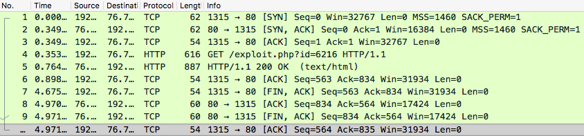
Figure 5-3. Attacker’s TCP session (source: Wireshark screen capture)
We can immediately extract basic information about the session, such as the following:
-
Session duration: 4.971 secs
-
Total session packets: 10
-
Protocol: TCP
-
Total bytes from source to destination:
- 62 + 54 + 616 + 54 + 54 + 54 = 894 bytes
-
Total bytes from destination to source:
- 62 + 887 + 60 + 60 = 1069 bytes
-
Successful TCP handshake: true
-
Network service on the destination: HTTP
-
Number of ACK packets: 4
Aggregating patterns across large sequences of packets can allow you to generate more useful information from the data than analyzing single packets. For instance, trying to detect SQL injections over the network by doing analysis on the packet level will cause you to look at a lot of useless packets due to protocol communication overhead. On the other hand, trying to detect Internet Control Message Protocol (ICMP) flooding DoS attacks requires analysis on the packet level because there are no sessions to speak of.
Other application-specific features can be extracted from network packet captures. For instance, you can extract messages issued over the Telnet protocol, as demonstrated in Figure 5-4.
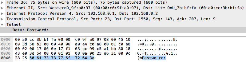
Figure 5-4. Data section of Telnet packet (source: Wireshark screen capture)
In this Telnet data packet, we see a password prompt. Telnet is a protocol designed for bidirectional interaction between two hosts with a virtual terminal connection. All Telnet is sent in the clear over the network, which is a huge security risk. In the early days of computer networking, this was not such a big concern. As security became a bigger issue, the SSH protocol eventually rose to replace Telnet. SSH implements strong encryption protocols that prevent interhost communication from being snooped on or hijacked. Nevertheless, Telnet, along with other unencrypted interhost communication protocols, remains in use within private networks, where security is assumed to be less of a concern.8 Application-level features extracted from known protocols such as Telnet can be very powerful for packet capture data analysis. Even in the case of encrypted communications, it can be worthwhile to decrypt the packets for feature extraction (using similar methods to terminating TLS/SSL, as we described earlier). Here are some examples of features that you can extract:
-
Application protocol (e.g., Telnet, HTTP, FTP, or SMTP)
-
Encrypted
-
Failed login attempt
-
Successful login attempt
-
Root access attempted (e.g.,
su rootcommand issued) -
Root access granted
-
Is guest login
-
curl/wget command attempted
-
File creation operation made
As discussed in previous chapters, the continuous or discrete features that you extract can be represented in feature vectors and conveniently used in data analysis and machine learning algorithms for information extraction.
Threats in the Network
Before we look at an example of network data analysis, it is important to discuss the threat model. As mentioned earlier, we will analyze attacks relevant to only the network, transport, and session layers (OSI layers 3, 4, and 5, respectively). Even though physical layer (layer 1 [L1]) and data link layer (layer 2 [L2]) attacks are important to consider in general discussions of network security, we omit them in our current analysis because the implementation and security of L1 and L2 fall outside the scope of application developers and security engineers. As such, implementing defenses on those layers is typically unfeasible unless you specialize in designing and developing network devices or software.
We broadly categorize threats into passive and active attacks, and further break down active attacks into four classes: breaches, spoofing, pivoting (“lateral movement”), and denial of service (DoS).
Passive attacks
Passive network attacks do not initiate communication with nodes in the network and do not interact with or modify network data. Attackers typically use passive techniques for information gathering and reconnaissance activity. Port scanning is a passive network attack that bad actors use to probe for open ports to identify services running on servers. Given knowledge of certain services’ or applications’ default ports, an adversary can learn what a server is running just based on its open ports; for example, an open port 27017 suggests a running MongoDB instance. Internet wiretapping (explained in the following sidebar) is a form of passive attack that manifests itself on the physical layer.
Active attacks
Active attacks are much more varied and can be further categorized into the following:
- Breaches
-
Network breaches are perhaps the most prolific network attacks. The term “breach” can refer to either a hole in the internal network’s perimeter or the act of an attacker exploiting such a hole to gain unauthorized access to private systems. For many server infrastructures, network nodes lie at the perimeter; routers, proxies, firewalls, switches, and load balancers are examples of such nodes. Intrusion detection systems are a form of perimeter defense that attempts to detect when an attacker is actively exploiting perimeter vulnerabilities to gain access to the network. As discussed in Chapter 3, intrusion detection systems are a common use case for anomaly detection.
Attackers can force their way into networks after performing passive information gathering and reconnaissance, finding vulnerabilities in publicly accessible endpoints that allow them shell or root access to systems. Commands issued over the network that attempt to exploit application vulnerabilities can be detected by inspecting communications between servers, which is why remote application attacks are sometimes classified as network breach attacks. For instance, buffer or heap overflow attacks, SQL injections, and cross-site scripting (XSS) attacks are not fundamentally caused by problems with the network; however, by inspecting traffic between hosts, network security systems can potentially detect such attempts to breach servers within the network. For example, basic remote buffer overflow attempts can be detected by inspecting network packet content for particular attack signatures and blocking or putting suspicious packets into quarantine. Nevertheless, polymorphism in such remotely launched attacks has rendered the method of checking attack signatures essentially useless. This is an area in which employing machine learning for fuzzy matching can help to change the game.
Data breaches by insiders also pose a significant network threat. Insider threat detection aims to detect when legitimate human actors within a system compromise that system (e.g., a corrupt employee trying to sell business secrets to competitors). Insider threats are a particularly tricky problem because system administrators typically have unfettered access to the infrastructure and can also be in control of security systems that prevent illegitimate attempts to access valuable data. We can reduce the attack surface by setting up proper role-based access control policies and a system of checks and balances for controlling and auditing internal security systems as well as encrypting stored data. Approaching the problem with data science, we can also view detecting insider threats as a classification or anomaly detection problem, looking for inconsistencies in access patterns to detect when a trusted user might be compromised.
- Spoofing
-
Attackers use spoofing (i.e., sending falsified data) as a mechanism for installing their presence in the middle of a trusted communications channel between two entities. DNS spoofing and ARP spoofing (also known as cache poisoning) misuse network caching mechanisms to force the client to engage in communications with a spoofed entity instead of the intended entity. By pretending to be the intended receiving party, attackers can then engage in passive wiretapping attacks to exfiltrate information from otherwise confidential communications.
DNS servers translate human-readable domains (e.g., www.example.com) to server IP addresses via the DNS resolution protocol. A network attacker can poison the client’s DNS cache by temporarily directing the client to an illegitimate DNS server which responds to the DNS resolution request with a malicious IP address. DNSSEC was introduced to guarantee authentication and integrity in the DNS resolution process, which prevents most DNS spoofing attacks.
- Pivoting
-
Pivoting is the technique of moving between servers in a network after an attacker has gained access to an entry point. Infrastructures in which the boundaries between services are improperly designed or configured are particularly susceptible to such attacks. Many high-profile data breaches have involved attackers pivoting through the network after gaining access to a low-value host. Low-value hosts are hosts within the network that don’t provide much information to the attackers even when breached. These are usually outward-facing systems such as web servers or point-of-sale terminals. By design, these systems do not store information that would be of value to attackers. Consequently, the security barriers around them are usually more relaxed compared to high-value systems such as business logic or customer databases.
In a well-designed secure network, communications between low-value hosts and high-value hosts should only be allowed through a small and controlled set of channels. However, many networks are not perfectly segmented, and contain blind spots that allow attackers to move from one virtual local area network (VLAN) to another, eventually finding their way to a high-value host. Techniques such as switch spoofing and double tagging allow attackers to perform VLAN hopping on inadequately configured VLAN interfaces. Attackers can also use a compromised low-value host to perform brute-force attacks, fuzzing, or port scanning on the rest of the network in order to find their next hop within the network. Meterpreter is a tool designed to automate the network pivoting process; you can use it in penetration testing to find pivoting vulnerabilities in your network.
- DoS
-
Denial-of-service (DoS) attacks target the general availability of a system, disrupting access to it by intended users. There are many flavors of DoS attacks, including the distributed DoS (DDoS) attack, which refers to the use of multiple IP addresses that might span a large range of geolocations to attack a service.
SYN flooding is a method of DoS that misuses the TCP handshake mechanism and exploits carelessly implemented endpoints. In the TCP three-way handshake process, every new TCP connection begins with the client sending a SYN packet to the server. The server responds to the client with a SYN-ACK packet and waits for a certain period of time for an ACK response from the client. The server must maintain a half-open connection while waiting for the ACK packet from the client, given that a delay in receiving packets could be due to a variety of reasons such as network connectivity or congestion issues. Maintaining these half-open connections consumes system resources for a certain period of time. Malicious clients can continually initiate TCP connections by flooding the server with SYN packets and not respond with ACKs, eventually draining the server of its finite resources and preventing legitimate clients from initiating connections.9 There are many other flavors of DoS attacks that similarly drain servers of available resources in order to interrupt service availability.
A botnet is a network of compromised privately owned computers that are infected (without the owners’ knowledge) with malicious software and used for remote access. Botnets have multiple uses, including sending spam, performing click fraud,10 and scraping web content, but a common use is to launch DDoS attacks. The importance of botnets is such that we will use the next section to examine them in greater detail.
Botnets and You
Half of all web traffic is generated by bots. Bots take on many forms, sometimes as simple as a Bash script consisting of curl commands; sometimes as a scripted headless browser such as PhantomJS; or sometimes even as a large-scale distributed web crawler powered by a framework like Apache Nutch. These bots are sometimes docile, crawling websites to index a search engine and abiding by the rules defined in a site’s robots.txt file. Other bots are not as respectful, and can even have malicious intent. One study concludes that 28.9% of all internet traffic can be attributed to malicious bots, though this number comes with a large margin of error. Bad bots perform illegitimate scraping of web content, stuff stolen credentials into login forms, engage in DDoS attacks, send spam and phishing emails, and more. As discussed in previous chapters, zombie machines in botnets (i.e., machines controlled remotely through the use of malware) are also referred to as bots, and they almost always have malicious intent. Large-scale botnets can enslave internet-connected computers around the world, allowing malicious controllers to amplify their activity without correspondingly scaling up their operational costs. Should distributed attacks originate from “bulletproof hosting services” located in jurisdictions historically involved with high levels of malicious traffic, web administrators can make a simple decision to block these low-reputation IP addresses or internet providers. However, botnets made up of home personal computers, from which large volumes of legitimate traffic can originate, can make the task of separating malicious and benign traffic much more difficult.
The importance of understanding botnets
It is important to know about botnets because of the large security risk they pose to enterprise networks and organizations. Zombies that are part of a network might not be considered active network attackers, but can have equally damaging consequences when the botnet is activated. Similar to APT attackers and network intruders, botnet zombies can launch insider attacks that leak important information, degrade system integrity, and wreak havoc in your environment. Learning about botnet topology and how bots work can help you to understand what to look for when trying to find infected hosts in your network.
Even though we will not discuss specific botnet detection techniques in this book, machine learning and statistical methods have played an important role in the fight against bots. You can use DNS query analysis11 or pattern mining to look for characteristics of network traffic that indicate autonomous bot behavior. Bots that use fast flux networks to mask command-and-control (C&C) servers can also be detected with machine learning.12 Additionally, clustering techniques have been applied to network traffic captures to detect zombie-to-C&C communications based on knowledge of botnet topologies.13,14
How do botnets work?
Botnets are distributed systems through and through. Because of the high monetary stakes, these systems often have elegant, fault-tolerant, and highly available architectures that can stand up to any do-gooders trying to shut them down. Zombie machines in the botnets (i.e., the bots) are typically controlled by task delegators (C&C servers). When a computer is infected by botnet malware, one of the first things that happens is the installation of some hidden daemon process that awaits instructions from a C&C server. In many ways, this process is coherent with modern server orchestration architectures. The first botnets made use of Internet Relay Chat (IRC) protocols to communicate with the C&C. Upon infection, an IRC daemon (IRCd) server15 process would be spun up, awaiting instructions on a predetermined channel. The botnet administrator could then issue commands on these channels, along the lines of the following:16
> ddos.synflood [host] [time] [delay] [port]
> (execute|e) [path]
> cvar.set spam_maxthreads [8]cvar
> spam.start
IRC was an easy choice in the early days of botnets because of its ubiquity and ease of deployment. In addition, it was a technology with which botnet miscreants were familiar, as a large amount of underground activity happens in IRC channels. The evolution of botnet topologies over time demonstrates how architectures can improve their fault tolerance and resilience. In general, there are four categories of C&C architectures:
- Star/centralized networks
-
The traditional method of botnet C&C (Figure 5-5) uses the simplest architecture in the playbook: a single centralized C&C server issuing commands to all zombies. This topology, called the star topology, allows for the most direct communications with zombies, but is obviously brittle because there is a single point of failure in the system. If the C&C server were to be taken down, the administrators would no longer have access to the zombies. Zombies in this configuration commonly use DNS as a mechanism for finding their C&C server, because the C&C addresses have to be hardcoded into the botnet application, and using a DNS name instead of an IP address allows for another layer of indirection (i.e., flexibility) in this frequently changing system.
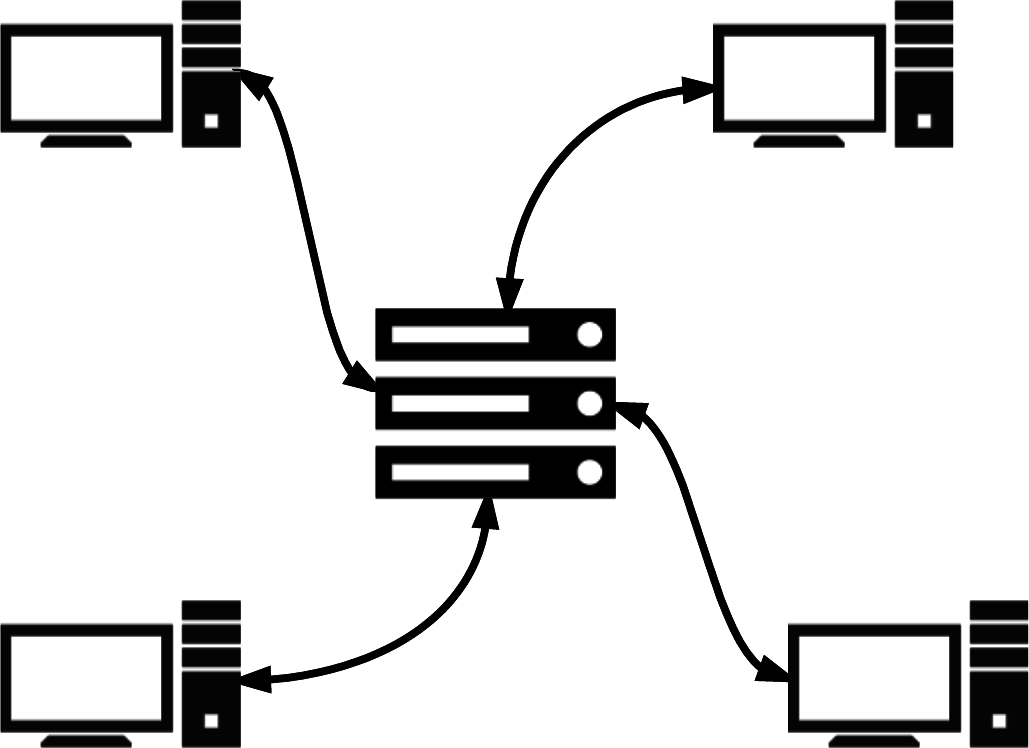
Figure 5-5. Star/centralized botnet C&C network diagram
Security researchers began detecting botnet zombies within the network by looking for suspicious-looking DNS queries.17 If you saw the following DNS query request served to the local DNS resolver, you might be tipped off to a problem:
Domain Name System (query)
    Questions: 1
    Answer RRs: 0
    Authority RRs: 0
    Additional RRs: 0
    Queries
        botnet-cnc-server.com: type A, class IN
            Name: botnet-cnc-server.com
            Type: A (Host address)
            Class: IN (0x0001)
As with families of malware that “phone home” to a central server, botnets had to adopt domain generation algorithms18 (DGAs) to obfuscate the DNS queries, making a resolution request instead to a DNS name like pmdhf98asdfn.com, which is more difficult to accurately flag as suspicious. Of course, security researchers then began to develop heuristics19 and statistical/machine learning models20 to detect these artificially generated DNS names, while botnet authors continued to try to make these domains look as innocuous as possible. This is another example of the typical cat-and-mouse game playing out.
- Multileader networks
-
The multileader botnet topology is quite similar to the centralized C&C topology, but is specifically engineered to remove the single point of failure. As we can see in Figure 5-6, this topology significantly increases the level of complexity of the network: C&C servers must frequently communicate between one another, synchronization becomes an issue, and coordination in general requires more effort. On the other hand, the multileader topology can also alleviate problems arising from physical distance. For botnets that span large geographical regions, having zombies that are constantly communicating with a C&C server halfway around the world is a source of inefficiency and increases the chance of detection because each communication consumes more system resources. Distributing C&C servers around the globe, as content delivery networks do with web assets, is a good way to remedy this problem. Yet, there still has to be some kind of DNS or server load balancing for zombies to communicate with the C&C cluster. Furthermore, this topology does not solve the problem of each zombie having to communicate with central command.
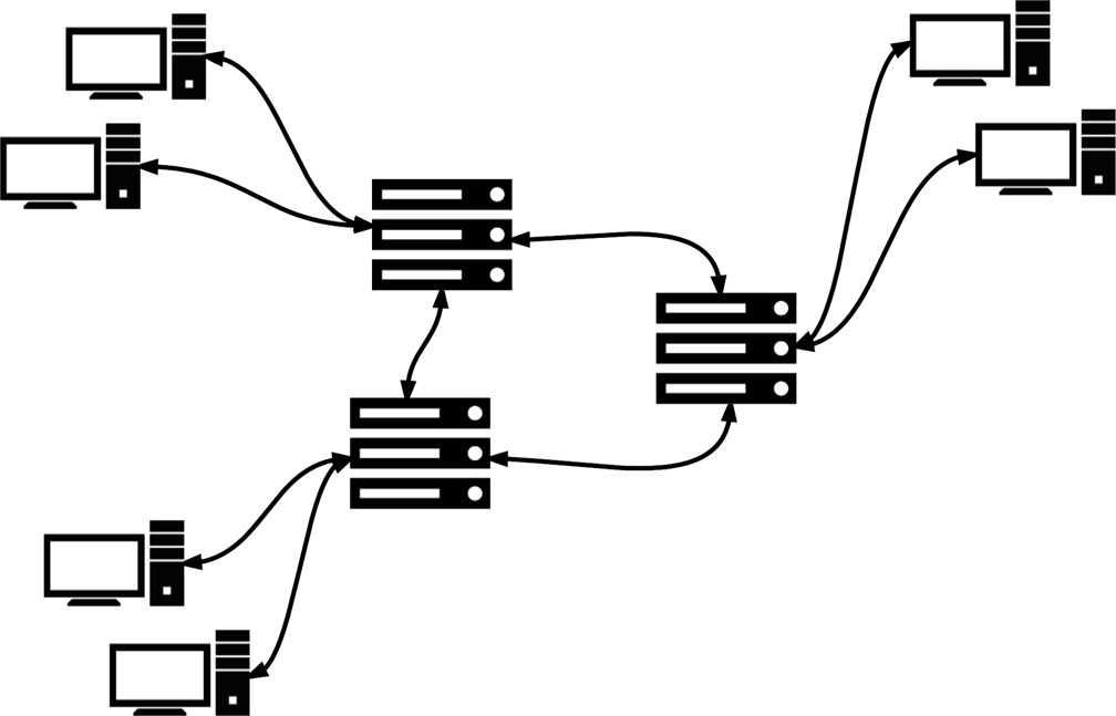
Figure 5-6. Multileader botnet C&C network diagram
- Hierarchical networks
-
Hierarchical C&C topologies were specifically designed to solve the problem of centralized command. As depicted in Figure 5-7, zombies are no longer just listeners, but can now also act as relays for upstream commands received. Botnet administrators can administer commands to a small group of directly connected zombies, which will then in turn propagate them to their child zombies, spreading the commands throughout the network. As you can imagine, tracing the source of commands is a gargantuan task, and this topology makes it very unlikely that the central C&C server(s) can be revealed. Nevertheless, because commands take time to propagate through the network, the topology might be unsuitable for activities that demand real-time reactions or responses. Furthermore, taking out a single zombie that happens to be high up in the propagation hierarchy can render a significant portion of the network unreachable by botnet administrators.
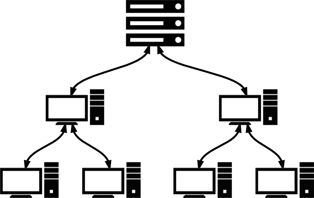
Figure 5-7. Hierarchical botnet C&C network diagram
- Randomized P2P networks
-
The next evolutionary step in botnet topology is a fully decentralized system of zombies, reminiscent of a peer-to-peer (P2P) network21 (see Figure 5-8). This topology removes any kind of central C&C mechanism and takes the concept of command relay to the extreme. Botnet administrators can issue commands to any bot or bots in the network and these commands are then propagated throughout the network, multicast style. This setup results in a highly resilient system because taking down an individual bot does not affect other bots in the network. That said, this topology does come with its fair share of complexities. The problem of command propagation latency is not solved, and it can be difficult to ensure that commands have been issued and acknowledged by all bots in the network because there is no centralized command or formal information flow protocol. In addition, botnet authors must design their command-issuing mechanism in a way that prevents their botnets from being taken over by rogue third parties. Because commands to control the botnet can be issued to any individual bot, including ones that might be located in unfavorable or untrusted execution environments (from the point of view of botnet administrators), a robust mechanism for ensuring the authenticity of the issued commands is important. A common way that this is achieved in modern P2P botnets is for administrators to sign commands with asymmetric cryptography, so authentication of commands can be performed in a decentralized and secure manner.
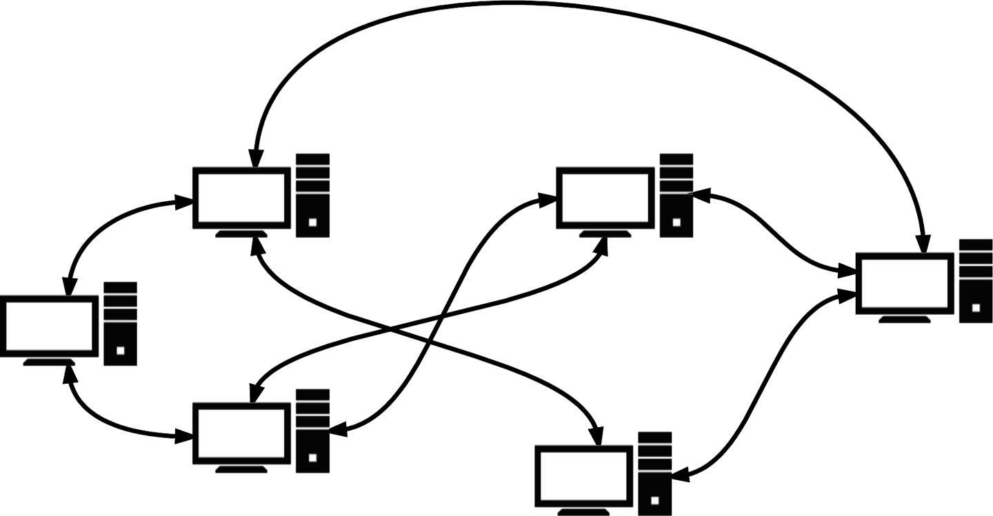
Figure 5-8. Randomized/P2P botnet C&C network diagram
Building a Predictive Model to Classify Network Attacks
In the remainder of this chapter, we demonstrate how to build a network attack classifier from scratch using machine learning. The dataset that we will use is the NSL-KDD dataset,22 which is an improvement to a classic network intrusion detection dataset used widely by security data science professionals.23 The original 1999 KDD Cup dataset was created for the DARPA Intrusion Detection Evaluation Program, prepared and managed by MIT Lincoln Laboratory. The data was collected over nine weeks and consists of raw tcpdump traffic in a local area network (LAN) that simulates the environment of a typical United States Air Force LAN. Some network attacks were deliberately carried out during the recording period. There were 38 different types of attacks, but only 24 are available in the training set. These attacks belong to four general categories:
dos-
Denial of service
r2l-
Unauthorized accesses from remote servers
u2r-
Privilege escalation attempts
probe-
Brute-force probing attacks
This dataset is somewhat artificial since is a labeled dataset consisting of pregenerated feature vectors. In many real scenarios, relevant labeled data might be difficult to come across, and engineering numerical features from the raw data will take up most of your effort.
Obtaining good training data is a perennial problem when using machine learning for security. Classifiers are only as good as the data used to train them, and reliably labeled data is especially important in supervised machine learning. Most organizations don’t have exposure to a large amount and wide variation of attack traffic, and must therefore figure out how to deal with the class imbalance problem. Data must be labeled by an oracle24 that can accurately classify a sample. In some cases, this labeling can be satisfied by operators without any special skills; for instance, labeling pictures of animals or sentiments of sentences. In the case of classifying network traffic, the task often must be carried out by experienced security analysts with investigative and forensic skills. The output of security operations centers can often be converted into some form of training data, but this process is very time consuming. In addition to using supervised learning methods to train our classifier, we will also experiment with using unsupervised methods, ignoring the training labels provided in the dataset.
With no good way to generate training data originating from the same source as the test data, another alternative is to train the classifier on a comparable dataset, often obtained from another source or an academic study. This method might perform well in some cases, but won’t in many. Transfer learning, or inductive transfer, is the process of taking a model trained on one dataset and then customizing it for another related problem. For example, transfer learning can take a generic image classifier25 that can distinguish a dress from a bag, and alter it to produce a classifier that can recognize different types of dresses. Transfer learning is currently an active research area, and there have been many successful applications of it in text classification,26 spam filtering,27 and Bayesian networks.28
As discussed in earlier chapters, building high-performing machine learning systems is a process filled with exploration and experimentation. In the next few sections, we walk through the process of understanding a dataset and preparing it for processing. Then, we present a few classification algorithms that we can apply to the problem. The focus of this exercise is not to bring you to the finish line of the task; rather, it is to get you through the heats and qualifiers, helping you get in shape to run the race.
Exploring the Data
Let’s begin by getting more intimate with the data on hand. The labeled training data as comma-separated values (CSV) looks like this:
0,tcp,ftp_data,SF,491,0,0,0,0,0,0,0,0,0,0,0,0,0,0,0,0,0,2,2,0.00,0.00,
0.00,0.00,1.00,0.00,0.00,150,25,0.17,0.03,0.17,0.00,0.00,0.00,0.05,
0.00,normal,20

0,icmp,eco_i,SF,8,0,0,0,0,0,0,0,0,0,0,0,0,0,0,0,0,0,1,21,0.00,0.00,
0.00,0.00,1.00,0.00,1.00,2,60,1.00,0.00,1.00,0.50,0.00,0.00,0.00,
0.00,ipsweep,17
The last value in each CSV record is an artifact of the NSL-KDD improvement that we can ignore. The class label is the second-to-last value in each record, and the other 41 values correspond to these features:
|
|
|
|
|
|
|
|
|
|
|
|
|
|
|
|
|
|
|
|
|
|
|
|
|
|
|
|
|
|
|
|
|
|
|
|
|
|
|
|
|
|
|
|
|
|
|
|
|
|
|
|
|
|
|
|
|
|
|
|
|
|
|
|
|
|
|
|
|
|
|
|
|
|
|
|
|
|
|
|
|
|
Our task is to devise a general classifier that categorizes each individual sample as one of five classes: benign, dos, r2l, u2r, or probe. The training dataset contains samples that are labeled with the specific attack: ftp_write and guess_passwd attacks correspond to the r2l category, smurf and udpstorm correspond to the dos category, and so on. The mapping from attack labels to attack categories is specified in the file training_attack_types.txt.29 Let’s do some preliminary data exploration to find out more about these labels. First, let’s take a look at the category distribution:30
fromcollectionsimportdefaultdict# The directory containing all of the relevant data filesdataset_root='datasets/nsl-kdd'category=defaultdict(list)category['benign'].append('normal')withopen(dataset_root+'training_attack_types.txt','r')asf:forlineinf.readlines():attack,cat=line.strip().split(' ')category[cat].append(attack)
Here’s what we find upon inspecting the contents of category:
{'benign':['normal'],'probe':['nmap','ipsweep','portsweep','satan','mscan','saint','worm'],'r2l':['ftp_write','guess_passwd','snmpguess','imap','spy','warezclient','warezmaster','multihop','phf','imap','named','sendmail','xlock','xsnoop','worm'],'u2r':['ps','buffer_overflow','perl','rootkit','loadmodule','xterm','sqlattack','httptunnel'],'dos':['apache2','back','mailbomb','processtable','snmpgetattack','teardrop','smurf','land','neptune','pod','udpstorm']}
We find that there are 41 attack types specified. This data structure is not very convenient for us to perform the mappings from attack labels to attack categories, so let’s invert this dictionary in preparation for data crunching:
attack_mapping=dict((v,k)forkincategoryforvincategory[k])
Now attack_mapping looks like this:
{'apache2':'dos','back':'dos','guess_passwd':'r2l','httptunnel':'u2r','imap':'r2l',...}
Here is the data that we are using:
train_file=os.path.join(dataset_root,'KDDTrain+.txt')test_file=os.path.join(dataset_root,'KDDTest+.txt')
It is always important to consider the class distribution within the training data and test data. In some scenarios, it can be difficult to accurately predict the class distribution of real-life data, but it is useful to have a general idea of what is expected. For instance, when designing a network attack classifier for deployment on a network that does not contain any database servers, we might expect to see very little sqlattack traffic. We can make this conjecture through educated guessing or based on past experience. In this particular example, we have access to the test data, so we can consume the data to get its distribution:
importpandasaspd# header_names is a list of feature names in the same order as the data# where the label (second-to-last value of the CSV) is named attack_type,# and the last value in the CSV is named success_pred# Read training datatrain_df=pd.read_csv(train_file,names=header_names)train_df['attack_category']=train_df['attack_type']\.map(lambdax:attack_mapping[x])train_df.drop(['success_pred'],axis=1,inplace=True)# Read test datatest_df=pd.read_csv(train_file,names=header_names)test_df['attack_category']=test_df['attack_type']\.map(lambdax:attack_mapping[x])test_df.drop(['success_pred'],axis=1,inplace=True)
Now let’s look at the attack_type and attack_category distributions:
importmatplotlib.pyplotasplttrain_attack_types=train_df['attack_type'].value_counts()train_attack_cats=train_df['attack_category'].value_counts()train_attack_types.plot(kind='barh')train_attack_cats.plot(kind='barh')
Figures 5-9 and 5-10 depict the training data class distributions.
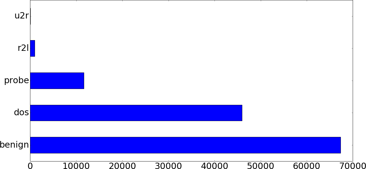
Figure 5-9. Training data class distribution (five-category breakdown)
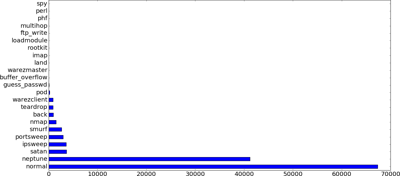
Figure 5-10. Training data class distribution (22-category breakdown)
The training data contains 22 types of attack traffic and the test data contains 37 types of attack traffic. The additional 15 types of attack traffic are not present in the training data. The dataset was designed in this way to test how well the trained classifier generalizes the training data. For example, let’s say that the classifier is able to correctly classify the worm attack into the r2l category even though the training data contained no worm attack samples. This means that this hypothetical classifier successfully learned some generalizable properties of the r2l category that allowed it to correctly classify previously unseen attack types belonging to this category.
One obvious observation is that the classes are tremendously imbalanced in both datasets. For instance, the u2r class is smaller than the dos class by three orders of magnitude in the training set. If we ignore this class imbalance and use the training data as is, there is a chance that the model will learn a lot more about the benign and dos classes compared to the u2r and r2l classes, which can result in an undesirable bias in the classifier. This is a very common problem in machine learning, and there are a few different ways to approach it. We will keep this drastic class imbalance in mind and address it later.
The original 1999 KDD Cup dataset was once widely used in network security and intrusion detection research but has since seen harsh criticism from researchers that found problems in using it for evaluating algorithms. Among these problems is the issue of high redundancy in the training and test datasets, causing artificially high accuracies in evaluating algorithms using this data. The NSL-KDD dataset that we are using addresses this issue. Another criticism is that this dataset is not a realistic representation of network traffic, so you should not use it for evaluating algorithms designed to be deployed in real network environments;31 the NSL-KDD dataset does not address this issue. For the purposes of this example, we are not concerned with how realistic this dataset is, because we are not evaluating algorithms to measure their effectiveness for use in real networks. The NSL-KDD dataset is a useful dataset for education and experimentation with data exploration and machine learning classification because it strikes a balance between simplicity and sophistication. The classification results that we get from the NSL-KDD dataset will not be as good as results that other publications using the original KDD dataset achieve (>90% classification accuracy).
Data Preparation
Let’s begin by splitting the test and training DataFrames into data and labels:
train_Y=train_df['attack_category']train_x_raw=train_df.drop(['attack_category','attack_type'],axis=1)test_Y=test_df['attack_category']test_x_raw=test_df.drop(['attack_category','attack_type'],axis=1)
Before we can apply any algorithms to the data, we need to prepare the data for consumption. Let’s first encode the categorical/dummy variables (referred to in the dataset as symbolic variables). For convenience, let’s generate the list of categorical variable names and a list of continuous variable names:32
feature_names=defaultdict(list)withopen(data_dir+'kddcup.names','r')asf:forlineinf.readlines()[1:]:name,nature=line.strip()[:-1].split(': ')feature_names[nature].append(name)
This gives us a dictionary containing two keys, continuous and symbolic, each mapping to a list of feature names:
{continuous:[duration,src_bytes,dst_bytes,wrong_fragment,...]symbolic:[protocol_type,service,flag,land,logged_in,...]}
We’ll further split the symbolic variables into nominal (categorical) and binary types because we will preprocess them differently.
Then, we use the pandas.get_dummies() function to convert the nominal variables into dummy variables. We combine train_x_raw and test_x_raw, run the dataset through this function, and then separate it into training and test sets again. This is necessary because there might be some symbolic variable values that appear in one dataset and not the other, and separately generating dummy variables for them would result in inconsistencies in the columns of both datasets.
It is typically not okay to perform preprocessing actions on a combination of training and test data, but it is acceptable in this scenario. We are neither doing anything that will prejudice the algorithm, nor mixing elements of the training and test sets. In typical cases, we will have full knowledge of all categorical variables either because we defined them or because the dataset provided this information. In our case, the dataset did not come with a list of possible values of each categorical variable, so we can preprocess as follows:33
# Concatenate DataFramescombined_df_raw=pd.concat([train_x_raw,test_x_raw])# Keep track of continuous, binary, and nominal featurescontinuous_features=feature_names['continuous']continuous_features.remove('root_shell')binary_features=['land','logged_in','root_shell','su_attempted','is_host_login','is_guest_login']nominal_features=list(set(feature_names['symbolic'])-set(binary_features))# Generate dummy variablescombined_df=pd.get_dummies(combined_df_raw,\columns=feature_names['symbolic'],\drop_first=True)# Separate into training and test sets againtrain_x=combined_df[:len(train_x_raw)]test_x=combined_df[len(train_x_raw):]# Keep track of dummy variablesdummy_variables=list(set(train_x)-set(combined_df_raw))
The function pd.get_dummies() applies one-hot encoding (discussed in Chapter 2) to categorical (nominal) variables such as flag, creating multiple binary variables for each possible value of flag that appears in the dataset. For instance, if a sample has value flag=S2, its dummy variable representation (for flag) will be:
# flag_S0, flag_S1, flag_S2, flag_S3, flag_SF, flag_SH[0,0,1,0,0,0]
For each sample, only one of these variables can have the value 1; hence the name “one-hot.” As mentioned in Chapter 2, the drop_first parameter is set to True to prevent perfect multicollinearity from occurring in the variables (the dummy variable trap) by removing one variable from the generated dummy variables.
Looking at the distribution of our training set features, we notice something that is potentially worrying:
train_x.describe()
| duration | src_bytes | … | hot | num_failed_logins | num_compromised | |
|---|---|---|---|---|---|---|
mean |
287.14465 |
4.556674e+04 |
0.204409 |
0.001222 |
0.279250 |
|
std |
2604.51531 |
5.870331e+06 |
2.149968 |
0.045239 |
23.942042 |
|
min |
0.00000 |
0.000000e+00 |
0.000000 |
0.000000 |
0.000000 |
|
… |
… |
… |
… |
… |
… |
|
max |
42908.00000 |
1.379964e+09 |
77.000000 |
5.000000 |
7479.000000 |
The distributions of each feature vary widely, which will affect our results if we use any distance-based methods for classification. For instance, the mean of src_bytes is larger than the mean of num_failed_logins by seven orders of magnitude, and its standard deviation is larger by eight orders of magnitude. Without performing feature value standardization/normalization, the src_bytes feature would dominate, causing the model to miss out on potentially important information in the num_failed_logins feature.
Standardization is a process that rescales a data series to have a mean of 0 and a standard deviation of 1 (unit variance). It is a common, but frequently overlooked, requirement for many machine learning algorithms, and useful whenever features in the training data vary widely in their distribution characteristics. The scikit-learn library includes the sklearn.preprocessing.StandardScaler class that provides this functionality. For example, let’s standardize the duration feature. As we just saw, the descriptive statistics for the duration feature are as follows:
> train_x['duration'].describe()

count    125973.00000
mean        287.14465
std        2604.51531
min           0.00000
25%           0.00000
50%           0.00000
75%           0.00000
max       42908.00000
Let’s apply standard scaling on it:
from sklearn.preprocessing import StandardScaler

# Reshape to signal to scaler that this is a single feature
durations = train_x['duration'].reshape(-1, 1)

standard_scaler = StandardScaler().fit(durations)
standard_scaled_durations = standard_scaler.transform(durations)
pd.Series(standard_scaled_durations.flatten()).describe()

> # Output:
count    1.259730e+05
mean     2.549477e-17
std      1.000004e+00
min     −1.102492e-01
25%     −1.102492e-01
50%     −1.102492e-01
75%     −1.102492e-01
max      1.636428e+01
Now, we see that the series has been scaled to have a mean of 0 (close enough: 2.549477 × 10⁻¹⁷) and standard deviation (std) of 1 (close enough: 1.000004).
An alternative to standardization is normalization, which rescales the data to a given range—frequently [0,1] or [−1,1]. The sklearn.preprocessing.MinMaxScaler class scales a feature from its original range to [min, max]. (The defaults are min=0, max=1 if not specified.) You might choose to use MinMaxScaler over StandardScaler if you want the scaling operation to preserve small standard deviations of the original series, or if you want to preserve zero entries in sparse data. This is how MinMaxScaler transforms the duration feature:
fromsklearn.preprocessingimportMinMaxScalermin_max_scaler=MinMaxScaler().fit(durations)min_max_scaled_durations=min_max_scaler.transform(durations)pd.Series(min_max_scaled_duration.flatten()).describe()># Output:count125973.000000mean0.006692std0.060700min0.00000025%0.00000050%0.00000075%0.000000max1.000000
Outliers in your data can severely and negatively skew standard scaling and normalization results. If the data contains outliers, sklearn.preprocessing.RobustScaler will be more suitable for the job. RobustScaler uses robust estimates such as the median and quantile ranges, so it will not be affected as much by outliers.
Whenever performing standardization or normalization of the data, you must apply consistent transformations to both the training and test sets (i.e., using the same mean, std, etc. to scale the data). Fitting a single Scaler to both test and training sets or having separate Scalers for test data and training data is incorrect, and will optimistically bias your classification results. When performing any data preprocessing, you should pay careful attention to leaking information about the test set at any point in time. Using test data to scale training data will leak information about the test set to the training operation and cause test results to be unreliable. Scikit-learn provides a convenient way to do proper normalization for cross-validation processes—after creating the Scaler object and fitting it to the training data, you can simply reuse the same object to transform the test data.
We finish off the data preprocessing phase by standardizing the training and test data:
fromsklearn.preprocessingimportStandardScaler# Fit StandardScaler to the training datastandard_scaler=StandardScaler().fit(train_x[continuous_features])# Standardize training datatrain_x[continuous_features]=\standard_scaler.transform(train_x[continuous_features])# Standardize test data with scaler fitted to training datatest_x[continuous_features]=\standard_scaler.transform(test_x[continuous_features])
Classification
Now that the data is prepared and ready to go, let’s look at a few different options for actually classifying attacks. To review, we have a five-class classification problem in which each sample belongs to one of the following classes: benign, u2r, r2l, dos, probe. There are many different classification algorithms suitable for a problem like this, and many different ways to approach the problem of multiclass classification. Many classification algorithms inherently support multiclass data (e.g., decision trees, nearest neighbors, Naive Bayes, multinomial logistic regression), whereas others do not (e.g., support vector machines). Even if our algorithm of choice does not inherently support multiple classes, there are some clever techniques for effectively achieving multiclass classification.
Choosing a suitable classifier for the task can be one of the more challenging parts of machine learning. For any one task, there are dozens of classifiers that could be a good choice, and the optimal one might not be obvious. In general, practitioners should not spend too much time deliberating over optimal algorithm choice. Developing machine learning solutions is an iterative process. Spending time and effort to iterate on a rough initial solution will almost always bring about surprising learnings and results. Knowledge and experience with different algorithms can help you to develop better intuition to cut down the iteration process, but it is rare, even for experienced practitioners, to immediately select the optimal algorithm, parameters, and training setup for arbitrary machine learning tasks. Scikit-learn provides a nifty machine learning algorithm cheatsheet gives a good overview of how to choose a machine learning algorithm.] that, though not complete, provides some intuition on algorithm selection. In general, here are some questions you should ask yourself when faced with machine learning algorithm selection:
-
What is the size of your training set?
-
Are you predicting a sample’s category or a quantitative value?
-
Do you have labeled data? How much labeled data do you have?
-
Do you know the number of result categories?
-
How much time and resources do you have to train the model?
-
How much time and resources do you have to make predictions?
Essentially, a multiclass classification problem can be split into multiple binary classification problems. A strategy known as one-versus-all, also called the binary relevance method, fits one classifier per class, with data belonging to the class fitted against the aggregate of all other classes. Another less commonly used strategy is one-versus-one, in which there are n_classes * (n_classes – 1) / 2 classifiers constructed, one for each unique pair of classes. In this case, during the prediction phase, each sample is run through all the classifiers, and the classification confidences for each of the classes are tallied. The class with the highest aggregate confidence is selected as the prediction result.
One-versus-all scales linearly with the number of classes and, in general, has better model interpretability because each class is only represented by one classifier (as opposed to each class being represented by n_classes – 1 classifiers for one-versus-one). In contrast, the one-versus-one strategy does not scale well with the number of classes because of its polynomial complexity. However, one-versus-one might perform better than one-versus-all with a classifier that doesn’t scale well with the number of samples, because each pairwise classifier contains a smaller number of samples. In one-versus-all, all classifiers each must deal with the entire dataset.
Besides its ability to deal with multiclass data, there are many other possible considerations when selecting a classifier for the task at hand, but we will leave it to other publications34 to go into these details. Having some intuition for matching algorithms to problems can help to greatly reduce the time spent searching for a good solution and optimizing for better results. In the rest of this section, we will give examples of applying different classification algorithms to our example. Even though it is difficult to make broad generalizations about when and how to use one algorithm over another, we will discuss some important considerations to have when evaluating these algorithms. By applying default or initial best-guess parameters to the algorithm, we can quickly obtain initial classification results. Even though these results might not be close to our target accuracy, they will usually give us a rough indication of the algorithm’s potential.
We first consider scenarios in which we have access to labeled training data and can use supervised classification methods. Then, we look at a semi-supervised and unsupervised classification methods, which are applicable whether or not we have labeled data.
Supervised Learning
Given that we have access to roughly 126,000 labeled training samples, supervised training methods seem like a good place to begin. In practical scenarios, model accuracy is not the only factor for which you need to account. With a large training set, training efficiency and runtime is also a big factor—you don’t want to find yourself spending too much time waiting for initial model experiment results. Decision trees or random forests are good places to begin because they are invariant to scaling of the data (preprocessing) and are relatively robust to uninformative features, and hence usually give good training performance.
If your data has hundreds of dimensions, using random forests can be much more efficient than other algorithms because of how well the model scales with high-dimensional data. Just to get a rough feel for how the algorithm does, we will look at the confusion matrix, using sklearn.metrics.confusion_matrix, and error rate, using sklearn.metrics.zero_one_loss. Let’s begin by throwing our data into a simple decision tree classifier, sklearn.tree.DecisionTreeClassifier:
fromsklearn.treeimportDecisionTreeClassifierfromsklearn.metricsimportconfusion_matrix,zero_one_lossclassifier=DecisionTreeClassifier(random_state=0)classifier.fit(train_x,train_Y)pred_y=classifier.predict(test_x)results=confusion_matrix(test_Y,pred_y)error=zero_one_loss(test_Y,pred_y)># Confusion matrix:[[93575929131][146760719800][696214151100][232541621912][17602715]]># Error:0.238245209368
With just a few lines of code and no tuning at all, a 76.2% classification accuracy (1 – error rate) in a five-class classification problem is not too shabby. However, this number is quite meaningless without considering the distribution of the test set (Figure 5-11).
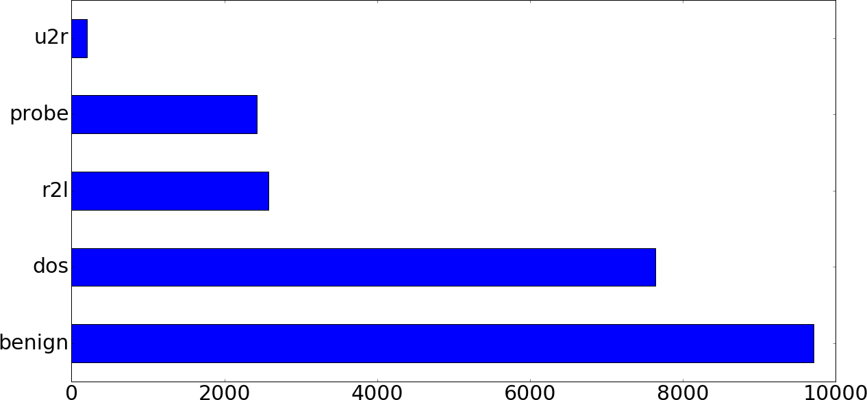
Figure 5-11. Test data class distribution (five-category breakdown)
The 5 × 5 confusion matrix might seem intimidating, but understanding it is well worth the effort. In a confusion matrix, the diagonal values (from the upper left to lower right) are the counts of the correctly classified samples. All the values in the matrix add up to 22,544, which is the size of the test set. Each row represents the true class, and each column represents the predicted class. For instance, the number in the first row and fifth column represents the number of samples that are actually of class 0 that were classified as class 4. (For symbolic labels like ours, sklearn assigns numbers in sorted ascending order: benign = 0, dos = 1, probe = 2, r2l = 3, and u2r = 4.)
Similar to the training set, the sample distribution is not balanced across categories:
>test_Y.value_counts().apply(lambdax:x/float(len(test_Y)))benign0.430758dos0.338715r2l0.114265probe0.107390u2r0.008872
We see that 43% of the test data belongs to the benign class, whereas only 0.8% of the data belongs to the u2r class. The confusion matrix shows us that although only 3.7% of benign test samples were wrongly classified, 62% of all test samples were classified as benign. Could we have trained a classifier that is just more likely to classify samples into the benign class? In the r2l and u2r rows, we see the problem in a more pronounced form: more samples were classified as benign than all other samples in those classes. Why could that be? Going back to look at our earlier analysis, we see that only 0.7% of the training data is r2l, and 0.04% is u2r. Compared with the 53.5% benign, 36.5% dos, and 9.3% probe, it seems unlikely that there would have been enough information for the trained model to learn enough information from the u2r and r2l classes to correctly identify them. To see whether this problem might be caused by the choice of the decision tree classifier, let’s look at how the k-nearest neighbors classifier, sklearn.neighbors.KNeighborsClassifier, does:
fromsklearn.neighborsimportKNeighborsClassifierclassifier=KNeighborsClassifier(n_neighbors=1,n_jobs=-1)classifier.fit(train_x,train_Y)pred_y=classifier.predict(test_x)results=confusion_matrix(test_Y,pred_y)error=zero_one_loss(test_Y,pred_y)># Confusion matrix:[[94555719324][167558946700][668156159700][234623715140][17704613]]># Error:0.240951029099
And here are the results for a linear support vector classifier, sklearn.svm.LinearSVC:
fromsklearn.svmimportLinearSVCclassifier=LinearSVC()classifier.fit(train_x,train_Y)pred_y=classifier.predict(test_x)results=confusion_matrix(test_Y,pred_y)error=zero_one_loss(test_Y,pred_y)># Confusion matrix:[[900629440533][196656601000][7141221497880][2464211090][17510816]]># Error:0.278167139815
The error rates are in the same ballpark, and the resulting confusion matrices show very similar characteristics to what we saw with the decision tree classifier results. At this point, it should be clear that continuing to experiment with classification algorithms might not be productive. What we can try to do is to remedy the class imbalance problem in the training data in hopes that resulting models will not be overly skewed to the dominant classes.
Class imbalance
Dealing with imbalanced classes is an art in and of itself. In general, there are two classes of remedies:
- Undersampling
-
Undersampling refers to sampling the overrepresented class(es) to reduce the number of samples. Undersampling strategies can be as simple as randomly selecting a fraction of samples, but this can cause information loss in certain datasets. In such cases, the sampling strategy should prioritize the removal of samples that are very similar to other samples that will remain in the dataset. For instance, the strategy might involve performing k-means clustering on the majority class and removing data points from high-density centroids. Other more sophisticated methods like removing Tomek’s links35 achieve a similar result. As with all data manipulations, be cautious of the side effects and implications of undersampling, and look out for potential effects of too much undersampling if you see prediction accuracies of the majority classes decrease significantly.
- Oversampling
-
Oversampling, which refers to intelligently generating synthetic data points for minority classes, is another method to decrease the class size disparity. Oversampling is essentially the opposite of undersampling, but is not as simple as arbitrarily generating artificial data and assigning it to the minority class. We want to be cautious of unintentionally imparting class characteristics that can misdirect the learning. For example, a naive way to oversample is to add random samples to the dataset. This would likely pollute the dataset and incorrectly influence the distribution. SMOTE36 and ADASYN37 are clever algorithms that attempt to generate synthetic data in a way that does not contaminate the original characteristics of the minority class.
Of course, you can apply combinations of oversampling and undersampling as desired, to mute the negative effects of each. A popular method is to first oversample the minority class and then undersample to tighten the class distribution discrepancy.
Class imbalance is such a ubiquitous problem that there are software libraries dedicated to it. Imbalanced-learn offers a wide range of data resampling techniques for different problems. Similar to classifiers, different resampling techniques have different characteristics and will vary in their suitability for different problems. Diving in and trying things out is a good strategy here. Note that some of the techniques offered in the imbalanced-learn library are not directly applicable to multiclass problems. Let’s first oversample using the imblearn.over_sampling.SMOTE class:
>(pd.Series(train_Y).value_counts())># Original training data class distribution:benign67343dos45927probe11656r2l995u2r52fromimblearn.over_samplingimportSMOTE# Apply SMOTE oversampling to the training datasm=SMOTE(ratio='auto',random_state=0)train_x_sm,train_Y_sm=sm.fit_sample(train_x,train_Y)(pd.Series(train_Y_sm).value_counts())># Training data class distribution after first SMOTE:benign67343dos67343probe67343u2r67343r2l67343
The ratio='auto' parameter passed into the imblearn.over_sampling.SMOTE constructor represents the strategy of oversampling all nonmajority classes to be the same size as the majority class.
With some experimentation, we find that random undersampling of our training data gives the best validation results. The imblearn.under_sampling.RandomUnderSampler class can help us out with this:
fromimblearn.under_samplingimportRandomUnderSamplermean_class_size=int(pd.Series(train_Y).value_counts().sum()/5)ratio={'benign':mean_class_size,'dos':mean_class_size,'probe':mean_class_size,'r2l':mean_class_size,'u2r':mean_class_size}rus=RandomUnderSampler(ratio=ratio,random_state=0)train_x_rus,train_Y_rus=rus.fit_sample(train_x,train_Y)>Originaltrainingdataclassdistribution:benign67343dos45927probe11656r2l995u2r52>AfterRandomUnderSamplertrainingdataclassdistribution:dos25194r2l25194benign25194probe25194u2r25194
Note that we calculated the mean class size across all 5 classes of samples and used that as the target size for undersampling. Now, let’s train the decision tree classifier with this resampled training data and see how it performs:
classifier=DecisionTreeClassifier(random_state=17)classifier.fit(train_x_rus,train_Y_rus)pred_y=classifier.predict(test_x)results=confusion_matrix(test_Y,pred_y)error=zero_one_loss(test_Y,pred_y)>Confusionmatrix:[[93697325865][1221576864700][270170198012][182923693695][620108219]]>Error:0.223962029808
Resampling helped us get from 76.2% accuracy to 77.6% accuracy. It’s not a huge improvement, but significant considering we haven’t started doing any parameter tuning or extensive experimentation yet.
Matching your task to the ideal classifier is sometimes tedious, but can also be fun. Through the process of experimentation, you will almost always find something unexpected and learn something new about your data, the classifier, or the task itself. However, iterating with different parameters and classifiers will not help if the dataset has fundamental limitations, such as a dearth of informative features.
As discussed earlier, labeled training data is expensive to generate because it typically requires the involvement of human experts or physical actions. Thus, it is very common for datasets to be unlabeled or consist only of a tiny fraction of labeled data. In such cases, supervised learning might work if you choose a classifier with high bias, such as Naive Bayes. However, your mileage will vary because high-bias algorithms are by definition susceptible to underfitting. You might then need to look to semi-supervised or fully unsupervised methods.
Semi-Supervised Learning
Semi-supervised learning is a class of supervised machine learning algorithms and training methods that are designed to work with very small sets of labeled training data. Self-training38 is a good example that we can use to illustrate semi-supervised techniques. In a nutshell, these algorithms go through an inductive training process, first training an initial estimator with the small set of training data, and then running it over unlabeled data. From these initial results, the highest confidence predictions are extracted and added to the training set, labeled with the results from the previous round of prediction. This process is then repeated until the training set contains a satisfactory number of samples.
Self-training produces a reasonably sized training set that often turns out to perform quite well. Some other semi-supervised learning techniques rely on generative approaches to create artificial labeled data from existing samples (the same idea as in oversampling, discussed earlier), or on density- and graph-based methods for learning the data manifold. These techniques infer labels for initially unlabeled data points with a reasonable degree of confidence.
Scikit-learn provides the sklearn.semi_supervised.LabelPropagation and sklearn.semi_supervised.LabelSpreading classes that can help you implement semi-supervised learning solutions.39
Unsupervised Learning
What if you have no labeled data at all? Especially in some use cases in security, labeled training data can be prohibitively difficult to generate (e.g., binary analysis requiring hours of fingerprinting and study per sample, or incident investigation requiring huge resources and bureaucratic layers to triage). In these cases, unsupervised learning is the only suitable option. This powerful statistical method infers hidden latent structure from unlabeled training data. In the classification space, the overwhelmingly dominant class of methods for unsupervised learning is clustering.
As we have discussed in earlier chapters, clustering refers to techniques that group similar data samples together, by some definition of similarity. Each group of similar points is called a cluster, and each cluster represents the learned model of a category. There are dozens of clustering models that might each be suitable in different scenarios. Some methods require you to know the number of classes or centroids ahead of time (e.g., k-means clustering, Gaussian mixture models), whereas others don’t (e.g., mean shift clustering). This distinction is the most important factor to consider when choosing which clustering method to use.
Going through a brief exercise of performing clustering on the NSL-KDD dataset will quickly allow us to see how clustering is different from the supervised techniques that we saw before. In our example, we know that our data contains five categories of samples, so we will choose the k-means clustering algorithm for the task with k (the number of clusters) equal to 5. (DBSCAN40 is another highly popular choice for clustering but is more suited for data containing clusters of similar density and hence is unsuitable for this task.) Note that k-means works only with continuous features (see Chapter 2 for details), so we use only the continuous features in our dataset. We use the sklearn.cluster.KMeans class:
fromsklearn.clusterimportKMeanskmeans=KMeans(n_clusters=5).fit(train_x)pred_y=kmeans.predict(test_x)# Inspect the clustering results(pd.Series(pred_y).value_counts())>115262252110206932
The results are visibly different from what we got with supervised techniques. What we get as a result of k-means clustering is a certain number of clusters, where each cluster is labeled with an arbitrary index. In this particular case, notice that the test set contains only four clusters even though we specified n_clusters=5. It seems that the last cluster did not gain membership of any of the test data points, which is unsurprising given our earlier discussion of class imbalance. What is more interesting is how we evaluate the results of clustering algorithms. None of the clusters have labels associated with them because we didn’t—and never needed to—pass in any label information to the algorithm. Thus, evaluating results of clustering is not as simple as just comparing expected and predicted labels.
To evaluate our model, we compute how many benign samples are grouped into the same cluster, and how many samples of other classes are grouped into that cluster. Specifically, we compute two metrics, the completeness score and the homogeneity score. A cluster is complete (has completeness score 1) if all data points belonging to the same class (i.e., with the same class label) are clustered together. On the other hand, a cluster is homogeneous (has homogeneity score 1) if all data points that are clustered together belong to the same class. The V-measure, defined to be the harmonic mean of homogeneity and completeness, provides a convenient single metric for evaluation:
v_measure_score=2*(homogeneity*completeness)/(homogeneity+completeness)
We generate the evaluation scores for our k-means clustering applied to the NSL-KDD dataset as follows:
fromsklearn.metricsimportcompleteness_score,\homogeneity_score,v_measure_score('Completeness: {}'.format(completeness_score(test_Y,pred_y)))('Homogeneity: {}'.format(homogeneity_score(test_Y,pred_y)))('V-measure: {}'.format(v_measure_score(test_Y,pred_y)))>Completeness:0.403815151707>Homogeneity:0.263893938589>V-measure:0.319194009471
A V-measure score of 0.32 is a really bad result. It looks like the data in its current state is not suitable for unsupervised classification. Indeed, class imbalance is problematic in clustering, where algorithms rely on shared properties of data points to form (in the ideal case) tight clusters of similar points. The lack of information about minority classes can lead to minority clusters not being correctly formed at all, instead resulting in “rogue” clusters siphoning away membership from otherwise well-formed clusters.
Experimenting with data resampling methods can help solve these problems, but it is important to note that some classes of problems are fundamentally unsuitable for unsupervised learning. If the data does not contain clearly separable clusters of samples, clustering will be an uphill task. How can we find out? Visualization is always useful for getting an intuition for the data, and is especially useful for clustering. We want to plot the samples in some space and visually observe the clusters formed. Before we attempt to plot our data on a chart, let’s check how many dimensions/features we have:
>('Total number of features: {}'.format(len(train_x.columns)))Totalnumberoffeatures:119
We can’t possibly plot all 119 dimensions, so we will perform dimensionality reduction to reduce the data to a more palatable set of two dimensions for representation on two-dimensional Cartesian axes. Principal component analysis41 (PCA) is one common dimensionality reduction method. It is difficult to explain this process accurately without diving into its mathematical formulation, but what PCA effectively does is find a set of axes (principal components) in high-dimensional space that are ordered by the amount of variance in the data that they explain, from greatest variance to smallest. It follows that projecting the dataset onto the first few axes captures most of the information in the dataset.
Performing dimensionality reduction after PCA is then as simple as picking out the top n principal components and representing your data in those n dimensions. In most cases, when performing PCA for the purposes of dimensionality reduction for downstream classification or processing, you should select a sufficient number of principal components to capture a large proportion of the variance in your data. For plotting purposes, however, choosing the top two principal components will often be sufficient to give a good representation for understanding the data. We use sklearn.decomposition.PCA on our training dataset, labeling data points with ground truth labels (see Figure 5-12):
fromsklearn.decompositionimportPCApca=PCA(n_components=2)train_x_pca=pca.fit_transform(train_x)plt.figure()colors=['navy','turquoise','darkorange','red','purple']forcolor,catinzip(colors,category.keys()):plt.scatter(train_x_pca[train_Y==cat,0],train_x_pca[train_Y==cat,1],color=color,alpha=.8,lw=2,label=cat)plt.legend(loc='best',shadow=False,scatterpoints=1)plt.show()
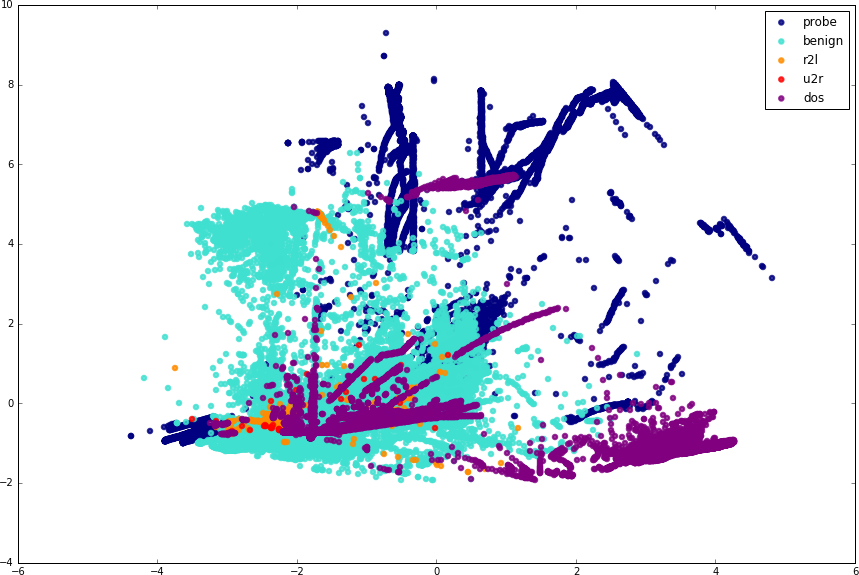
Figure 5-12. Scatter plot of training data with ground truth labels (transformed with PCA)
The first principal component is represented on the horizontal axis, and the second is represented on the vertical axis. It is easy to see that this dataset is not very suitable for clustering. The probe, dos, and r2l samples are scattered unpredictably, and do not form any strong clusters. Because there are few u2r samples, it is difficult to observe this class on the plot and it does not form any visible clusters. Only benign samples seem to form a strong cluster. To satisfy our curiosity, let’s plot these same points with the labels assigned after fitting them to the k-means clustering algorithm that we used earlier:
fromsklearn.clusterimportKMeans# Fit the training data to a k-means clustering estimator modelkmeans=KMeans(n_clusters=5,random_state=17).fit(train_x)# Retrieve the labels assigned to each training samplekmeans_y=kmeans.labels_# Plot in 2d with train_x_pca_contplt.figure()colors=['navy','turquoise','darkorange','red','purple']forcolor,catinzip(colors,range(5)):plt.scatter(train_x_pca_cont[kmeans_y==cat,0],train_x_pca_cont[kmeans_y==cat,1],color=color,alpha=.8,lw=2,label=cat)plt.legend(loc='best',shadow=False,scatterpoints=1)plt.show()
Figure 5-13 shows the result.
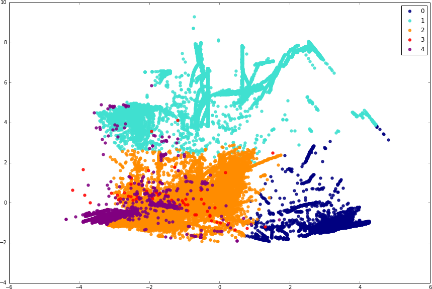
Figure 5-13. Scatter plot of training data with k-means predicted classes (k=5)
Now, remember that the k-means algorithm is unsupervised, so it is not aware of which label each formed cluster corresponds to. Immediately, in Figure 5-13, we can observe significant differences in the clusters formed by k-means and the ground truth clusters. The algorithm performs well in grouping certain sections of the data together, but it fails to group together clusters of the dos label and wrongly classifies a large section of “benign” traffic as attack traffic (the upper-left section of Figure 5-13). Tuning and experimenting with the value of k can help with this, but from this brief visual analysis, we see that there might be some fundamental problems with using only clustering methods to classify network attacks in this data.
Even when we are just using continuous features, we are still dealing with a dataset comprising 34 dimensions. Recall from Chapter 2 that k-means loses effectiveness in high dimensions. This is a problem that we can solve by feeding the algorithm with dimensionality-reduced (e.g., with PCA) data. However, something that is more difficult to solve is the inherent distribution characteristics. In Chapter 2, we also mentioned that k-means does not work well on nonspherical distributions. From Figure 5-12, it is difficult to argue that any of the classes have a spherical distribution. No wonder k-means does not work well here!
Advanced Ensembling
k-means works relatively well in assigning labels to some contiguous clusters of data. Trying out k-means with k=8, we get the result illustrated in Figure 5-14.
Comparing this plot with the ground truth labels in Figure 5-12, we notice that some clusters of data do mostly belong to the same class. Other clusters, such as cluster 2, seem to be made up of a mix of benign and probe traffic. If there were a way to perform further classification within clusters, we might be able to achieve better results. This intuition is leading us to a well-known class of techniques known as ensembling.
Ensembling techniques (or ensemble models) refer to the combination of two or more machine learning models (they could use the same underlying algorithm or altogether different algorithms) to form a single system.42 The goal is to combine the results of multiple weak models to form a single stronger learner.
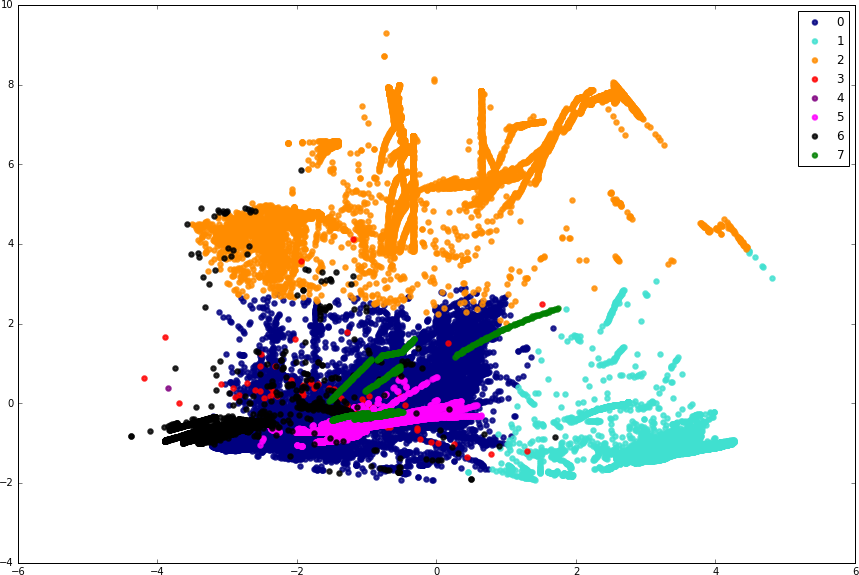
Figure 5-14. Scatter plot of training data with k-means predicted classes (k=8)
In our example, we are trying to perform further classification separately on some clusters that contain mixed labels, attempting to partition these clusters better than k-means would have been able to. To simplify the problem, let’s attempt to classify this network traffic into just the two classes that matter most: attack and benign traffic. We reduce the dimensionality of the problem by using a method of ranking features called the attribute ratio.43 We do not go into further detail here,44 but we used this feature ranking method to select the features with an attribute ratio greater than 0.01, which reduces the number of features we will use to 31. Let’s first define the labels for our task:
train_Y_bin=train_Y.apply(lambdax:'benign'ifx=='benign'else'attack')
Then, we select the subset of important features, apply k-means on it with k=8, and observe the cross-tabulation of the eight k-means clusters and the ground truth binary labels (Table 5-1):
kmeans=KMeans(n_clusters=8,random_state=17).fit(train_df_ar_trimmed[continuous_features_trimmed])kmeans_train_y=kmeans.labels_pd.crosstab(kmeans_train_y,train_Y_bin)
| attack category | attack | benign |
|---|---|---|
0 |
6457 |
63569 |
1 |
11443 |
2784 |
2 |
34700 |
126 |
3 |
0 |
1 |
4 |
4335 |
628 |
5 |
757 |
167 |
6 |
884 |
0 |
7 |
54 |
68 |
Looking at Table 5-1, we must consider how we want to deal with each cluster. Notice how clusters 2 and 6 have a very clear majority of attack traffic, clusters 3 and 7 seem to contain only low levels of noise, and the rest of the clusters are quite mixed. Developing a suitable result aggregation strategy from the training data is a crucial step in ensembling, and it is worthwhile spending time to experiment with which approach works best. For this example, we devise a three-path strategy for dealing with each cluster:
-
For clusters that have an aggregate size of fewer than 200 samples, we consider them outliers and assign them the
attacklabel. -
For clusters with more than 99% of samples belonging to a single class (either
attackorbenign), we assign the dominant label to the entire cluster. -
For each of the remaining clusters, we train a separate decision tree classifier.
According to this strategy, clusters 3 and 7 will be considered “noise” and be assigned the attack label. Clusters 2 and 6 both have more than 99% of the traffic classified as attacks so that label propagates to the entire cluster. We will train decision tree classifiers for each of clusters 0, 1, 4, and 5.
We evaluate our method by first running the test samples through the k-means model to obtain the test clusters. Then, all the test samples assigned to clusters 2, 3, 6, and 7 will immediately be labeled as attack. Test samples assigned to cluster 0 will be put through the decision tree classifiers trained on cluster 0 from the training set, and so on.
As an example, here is how we train cluster 4’s decision tree classifier and make predictions on test cluster 4’s samples:
train_y4=train_df[train_df.kmeans_y==4]test_y4=test_df[test_df.kmeans_y==4]dfc4=DecisionTreeClassifier(random_state=17).fit(train_y4.drop(['kmeans_y'],axis=1),train_y4['labels2'])dtc4_pred_y=dtc4.predict(test_y4.drop(['kmeans_y'],axis=1))
Following our aggregation strategy, Table 5-2 lists the combined test set confusion matrices for all eight clusters.
| Predicted benign | Predicted attack | |
|---|---|---|
Actual benign |
9,418 |
293 |
Actual attack |
4,020 |
8,813 |
Analyzing the classification report, we see the results listed in Table 5-3.
| Precision | Recall | F1 score | Support | |
|---|---|---|---|---|
benign |
0.70 |
0.97 |
0.81 |
9711 |
attack |
0.97 |
0.69 |
0.80 |
12833 |
Where:
-
Precision = True Positives / (True Positives + True Negatives)
-
Recall = True Positives/ (True Positives + False Negatives)
In other words, precision is the proportion of the predicted items that are relevant, and recall is the proportion of the relevant items that are correctly predicted.
We see that the precision for predicted attacks is 97%. This means that if the classifier predicts that a sample is an attack, there is a 97% chance that it actually is an attack. The recall for benign traffic is also 97%, which means that 97% of all actual benign traffic is correctly predicted as benign traffic.
The problematic parts of the results are the comparatively low precision for the benign traffic and low recall for attack traffic. In fact, 30% of the traffic that this classifier classifies as benign is actually an attack.
How can we explain these bad results for benign predictions? Let’s look at the k-means cross-tabulation for the test dataset and compare it with that of the training data:
# kmeans_test_y is clusters predicted by k-meanspd.crosstab(kmeans_test_y,test_Y_bin)
Table 5-4 shows the results.
| attack category | attack | benign |
|---|---|---|
0 |
9,515 |
4,795 |
1 |
87 |
5131 |
2 |
6 |
1,997 |
3 |
0 |
0 |
4 |
51 |
427 |
5 |
10 |
1 |
6 |
37 |
8 |
7 |
5 |
474 |
If we compare Table 5-1 to Table 5-4, we see that the biggest discrepancies between the attack/benign distributions within a single cluster come from cluster 0.45 In the training data, cluster 0 contains just 9% attack traffic, whereas in the test data, cluster 0 contains 66% attack traffic! It seems like the information that is captured by the k-means model for cluster 0 is insufficient to generalize to the test data. Let’s confirm this hypothesis by examining the confusion matrix for cluster 0’s decision tree classifier predictions, as shown in Table 5-5.
| Predicted benign | Predicted attack | |
|---|---|---|
Actual benign |
9,352 |
163 |
Actual attack |
3,062 |
1,733 |
Comparing Table 5-2 and Table 5-5, notice that 76% (3,062 out of 4,020) of the total false negative (predicted benign + actual attack) predictions made by the ensemble are caused by cluster 0’s decision tree classifier. If we could make cluster 0’s classifier better, we would greatly improve the ensemble classifier’s overall performance.
Now, you might be tempted to use these specific test results to improve your model. Perhaps you would be able to improve results by using a different algorithm just for cluster 0? In most cases, this kind of customization would be the cardinal sin of machine learning. You should be careful never to make adjustments to your model based on results from the test set.
However, consider the following scenario: suppose that you have this model in production for a month, and you observe that cluster 0’s decision tree classifier is consistently underperforming. Making changes to your model based on this information is okay—in fact, it is highly encouraged!
How is this different? Notice that in the latter case, you have expanded your training set to the data you have collected (and perhaps also labeled) over the course of the month. You can now use this newly defined training set to develop the next version of the classifier. However, note that you will also need to generate a test set corresponding to this new training set.
Conclusion
Having worked through the task in this chapter, it should be clear that machine learning—specifically, data correlation and classification—is about more than just choosing the right classifier and knowing about algorithms. Spending time to explore and understand the data is key, and can help save you precious time in getting to a desired classification accuracy. The security space provides some unique challenges when applying machine learning. More often than not, you will be faced with class imbalance and lack of training data. Sometimes, continuing to tune algorithms or the learning process may not be the answer—collecting more data, generating more descriptive features, changing class/category definitions, adjusting the learning goals, or all of the above might be what you need to obtain better results.
1 For the purposes of our discussion, we restrict the definition of “network” to be a system of connections that allows for the transmission of data between connected nodes. There is an enormous range of data transmission mediums, communication protocols, network topologies, and infrastructure setups that will affect any detailed discussion of network security, and we do not cover all this ground. Instead, we use a few important and common scenarios to drive the discussion. You will find that you can apply many of the general concepts and techniques discussed here to specific use cases and scenarios, even if there are some differences in the environment or protocols.
2 We use CIDR notation to refer to IP subnets.
3 David Wu, “Fully Homomorphic Encryption: Cryptography’s Holy Grail,” XRDS: Crossroads, The ACM Magazine for Students 21:3 (2015): 24–29.
4 Zvika Brakerski, Craig Gentry, and Vinod Vaikuntanathan, “Fully Homomorphic Encryption Without Bootstrapping,” Proceedings of the 3rd Innovations in Theoretical Computer Science Conference (2012): 309–325.
5 Packet analyzers exist in both hardware and software form and can capture either packet headers only or full contents.
6 See snakeoil2_070531.tgz, available at https://wiki.wireshark.org/SampleCaptures#Sample_Captures.
7 R.L. Rivest, A. Shamir, and L. Adleman, “A Method for Obtaining Digital Signatures and Public-Key Cryptosystems,” Communications of the ACM 21 (1978): 120–126.
8 In fact, many operating systems are still distributed with Telnet installed and activated by default. Administrators who intend to protect systems against Telnet attacks must explicitly disable the service or filter out Telnet traffic.
9 RFC 4987 describes SYN flooding attacks and recommends countermeasures to circumvent them.
10 Generating artificial clicks on an advertisement hosted on a website with the intention of generating fraudulent revenue for the host website and/or draining advertising budget from the advertiser.
11 Leyla Bilge et al., “EXPOSURE: A Passive DNS Analysis Service to Detect and Report Malicious Domains,” ACM Transactions on Information and System Security 16:4 (2014).
12 Z. Berkay Celik and Serna Oktug, “Detection of Fast-Flux Networks Using Various DNS Feature Sets,” IEEE Symposium on Computers and Communications (2013).
13 Guofei Gu et al., “BotMiner: Clustering Analysis of Network Traffic for Protocol- and Structure-Independent Botnet Detection”, Proceedings of the 17th USENIX Security symposium (2008): 139–154.
14 Florian Tegeler et al., “BotFinder: Finding Bots in Network Traffic Without Deep Packet Inspection”, Proceedings of the 8th International Conference on Emerging Networking Experiments and Technologies (2012): 349–360.
15 Examples of some IRC daemons are https://www.unrealircd.org/ and http://www.inspircd.org/.
16 Example botnet commands from Agobot, a popular IRC botnet, are described in “The Evolution of Malicious IRC Bots” by John Canavan of Symantec Security Response.
17 Christian Dietrich et al. “On Botnets That Use DNS for Command and Control,” Proceedings of the 7th European Conference on Computer Network Defense (2011): 9–16.
18 Phillip Porras, Hassen Saidi, and Vinod Yegneswaran, “An Analysis of Conficker’s Logic and Rendezvous Points,” SRI International Technical Report (2009).
19 Sandeep Yadav et al., “Detecting Algorithmically Generated Malicious Domain Names,” Proceedings of the 10th ACM SIGCOMM Conference on Internet Measurement (2010): 48–61.
20 Hyrum S. Anderson, Jonathan Woodbridge, and Bobby Filar, “DeepDGA: Adversarially-Tuned Domain Generation and Detection,” Proceedings of the 2016 ACM Workshop on Artificial Intelligence and Security (2016): 13–21.
21 Ping Wanget al., “A Systematic Study on Peer-to-Peer Botnets,” Proceedings of the 18th International Conference on Computer Communications and Networks (2009): 1–8.
22 Mahbod Tavallaee et al., “A Detailed Analysis of the KDD CUP 99 Data Set,” Proceedings of the 2nd IEEE Symposium on Computational Intelligence in Security and Defense Applications (2009): 53–58.
23 This is provided to you in chapter5/datasets in our code repository.
24 An oracle machine is defined in complexity and computability theory as an abstract entity that is able to solve problems with definitive correctness in a single operation.
25 The ImageNet deep neural network classifier has seen many successful applications using it as a base for transfer learning. For an exploration of what features about ImageNet make it so successful for this purpose, see Minyoung Huh, Pulkit Agrawal, and Alexei E. Efros, “What Makes ImageNet Good for Transfer Learning,” Berkeley Artificial Intelligence Laboratory, UC Berkeley (2016).
26 Chuong Do and Andrew Ng, “Transfer Learning for Text Classification,” Proceedings of the 18th International Conference on Neural Information Processing Systems (2005): 299–306.
27 Steffen Bickel, “ECML-PKDD Discovery Challenge 2006 Overview,” Proceedings of the ECML-PKDD Discovery Challenge Workshop (2006): 1–9.
28 Alexandru Niculescu-Mizil and Rich Caruana, “Inductive Transfer for Bayesian Network Structure Learning,” Proceedings of the 11th International Conference on Artificial Intelligence and Statistics (2007): 339–346.
29 This file is not included as part of the NSL-KDD dataset but is included in the original KDD 1999 dataset.
30 The code for the full example is provided as a Python Jupyter notebook at chapter5/nsl-kdd-classification.ipynb in our code repository.
31 John McHugh, “Testing Intrusion Detection Systems: A Critique of the 1998 and 1999 DARPA Intrusion Detection System Evaluations as Performed by Lincoln Laboratory,” ACM Transactions on Information and System Security 3 (2000): 262–294.
32 The kddcup.names file is not included in the NSL-KDD dataset, but only in the original KDD 1999 dataset.
33 We remove root_shell from the list of continuous features because this is an error in the dataset. The kddcup.names file wrongly marks “root_shell” as a continuous feature, whereas the dataset documentation clearly states that it is a binary feature. Furthermore, it is clear from exploring the data that this feature does not take on values other than 0 and 1. Hence, we treat this feature as a binary feature throughout this example.
34 A good reference is The Elements of Statistical Learning, 2nd ed., by Trevor Hastie, Robert Tibshirani, and Jerome Friedman (Springer).
35 Ivan Tomek, “Two Modifications of CNN,” IEEE Transactions on Systems, Man, and Cybernetics 6 (1976): 769–772.
36 N.V. Chawla et al., “SMOTE: Synthetic Minority Over-Sampling Technique,” Journal of Artificial Intelligence Research (2002): 321–357.
37 Haibo He et al., “ADASYN: Adaptive Synthetic Sampling Approach for Imbalanced Learning,” Proceedings of the IEEE International Joint Conference on Neural Networks (IEEE World Congress on Computational Intelligence) (2008): 1322–1328.
38 Yan Zhou, Murat Kantarcioglu, and Bhavani Thuraisingham, “Self-Training with Selection-by-Rejection,” Proceedings of the IEEE 12th International Conference on Data Mining (2012): 795–803.
39 We won’t be using semi-supervised learning in this example because it typically involves a lengthy process of analyzing similarities between clusters that is very specific to the dataset in use. For more details on semi-supervised learning, we highly recommend looking into Semi-Supervised Learning by Olivier Chapelle, Bernhard Schölkopf, and Alexander Zien (MIT Press).
40 Refer to Chapter 2 for more details. See also Martin Ester et al., “A Density-Based Algorithm for Discovering Clusters in Large Spatial Databases with Noise,” Proceedings of the 2nd ACM SIGKDD International Conference on Knowledge Discovery and Data Mining (1996): 226–231.
41 Svante Wold, Kim Esbensen, and Paul Geladi, “Principal Component Analysis,” Chemometrics and Intelligent Laboratory Systems 2 (1987): 37–52.
42 We do not go into all the details of ensembling techniques here. For a great reference on this subject, refer to Ensemble Machine Learning: Methods and Applications by Cha Zhang and Yunqian Ma (Springer Publishing).
43 Hee-su Chae and Sang Hyun Choi, “Feature Selection for Efficient Intrusion Detection Using Attribute Ratio,” International Journal of Computers and Communications 8 (2014): 134–139.
44 Complete implementation of the attribute ratio calculation is provided in the Using “Attribute Ratio” (AR) feature selection section of the Python Jupyter notebook found at chapter5/nsl-kdd-classification.ipynb in our code repository.
45 We acknowledge that there are also significant differences in the label distributions of clusters 5, 6, and 7, but the number of samples involved is relatively small compared with the size of the dataset. Hence, these discrepancies can be explained by noise in the dataset.