More About Metrics

In our discussion of clustering, we primarily used the standard Euclidean distance between vectors in a vector space:

Euclidean distance is also known as the L₂ norm. There are several other metrics that are commonly used in applications:

• One variation of Euclidean distance is the L₁ norm, also known as Manhattan distance (because it counts the number of “blocks” between two points on a grid):

  $$d(x,y)=\sum _i|(x_i-y_i)|$$

• Another is the L_∞ norm, defined as the following:

  $$d(x,y)=\underset{i}{\max }|(x_i-y_i)|$$

• For vectors of binary values or bits, you can use Hamming distance, which is the number of bits in common between x and y. This can be computed as:

  $$d(x,y)=H(\neg (x\oplus y\left)\right)$$

  where H(v) is the Hamming weight; that is, the number of “1” bits in v. If the points you compare are of different bit length, the shorter one will need to be prepended with zeros.

• For lists, you can use the Jaccard similarity:

  $$d(x,y)=\frac{|x\cap y|}{|x\cup y|}$$

  The Jaccard similarity computes the number of elements in common between x and y, normalized by the total number of elements in the intersection. One useful property of Jaccard similarity is that you can use it to compare lists of different lengths.

The L₁ and L₂ metrics in vector spaces suffer from what is known as the “curse of dimensionality.” This phrase refers to the principle that as the number of dimensions increases, all points seem to be roughly equally distant from one another. Thus, if you are trying to cluster items in high-dimensional space, you should either reduce the number of dimensions or use a different metric, such as the L_∞ norm. For a more formal treatment, see section 2.5 of The Elements of Statistical Learning, 2nd ed., by Trevor Hastie, Robert Tibshirani, and Jerome Friedman (Springer).

Size of Logistic Regression Models

Digging deeper into the contents of the LogisticRegression classifier object, you’ll notice that all that changed after the call to fit() is the assignment of the three attributes coef_, intercept_, and n_iter_. Let’s inspect these attributes and see what a logistic regression classifier model actually is:

print(clf.coef_)

> [[-7.44949492  0.26692309  1.39595031 −1.44011704  1.41274547
    1.32026309   0.20373255]]

print(clf.intercept_)

> [ 2.93674111]

print(clf.n_iter_)

> [19]

The n_iter_ attribute is irrelevant because it serves only to tell us the number of iterations of some training process that it took to train the classifier to its current state. This means that the entirety of the information learned from the training set is stored within the eight numpy.float64 numbers of coef_ and intercept_. Because each of the eight numpy.float64 objects is 8 bytes in size, the model can be fully represented using just 64 bytes of storage. The logistic regression model has managed to compress all the information about how to (almost) perfectly identify fraudulent transactions in this online retailer’s environment from the 26,728 data points in the training set into a mere 64 bytes.

Implementing the Logistic Regression Cost Function

The cost function for binary logistic regression is the product of the individual probabilities (or likelihoods) for each class:

This formula might look intimidating, but the general concept really isn’t that different from linear regression. Let’s break it down further.

Unlike linear regression, logistic regression is a regression model in which the dependent variable is categorical; that is, the value that we want to predict is discrete in nature. This is convenient for classification tasks because the output we want is one out of the n category labels. For example, the payment fraud classifier that we looked at a moment ago is a binary classifier whose output can be only either 0 or 1.

The error (derived from residuals) for a single point can then be expressed by using the log-likelihoods of the sigmoid function:

We can rewrite this expression as the following:

If h(x) is very close to 1, the loss is small when the true label is 1 and high when the true label is 0.

The cost function is simply the mean of all the errors in the training set:

When expanded, this gives us the aforementioned logistic regression cost function:

Minimizing the Cost Function

An intuitive way to think about minimizing the cost function is to consider a simpler form of supervised machine learning, linear regression, also known as least squares regression. Given a two-dimensional dataset, we want to fit a regression line (line of best fit, trend line) to capture the relationship between these two dimensions (on the x- and y-axes of the graph in Figure 2-4).

To do this, we first define a cost function that we will use as the objective in our optimization process. This cost function will give us a quantitative measure of how well this regression line is able to capture the linear relationship in the data. The cost function, as defined in the linear regression algorithm, is the sum of the squared residuals for every point in the dataset. The residual for a data point is the difference between the predicted and actual y-values, as illustrated in Figure A-1. Summing up all the squared residuals between a set of data points and a regression line gives us the cost of that particular line. The larger the value of the cost function, the worse the regression line is at capturing a linear relationship in the dataset. Hence, the optimization objective is to adjust the parameters of the linear regression model (i.e., the slope and intercept of the line) to minimize this cost function.

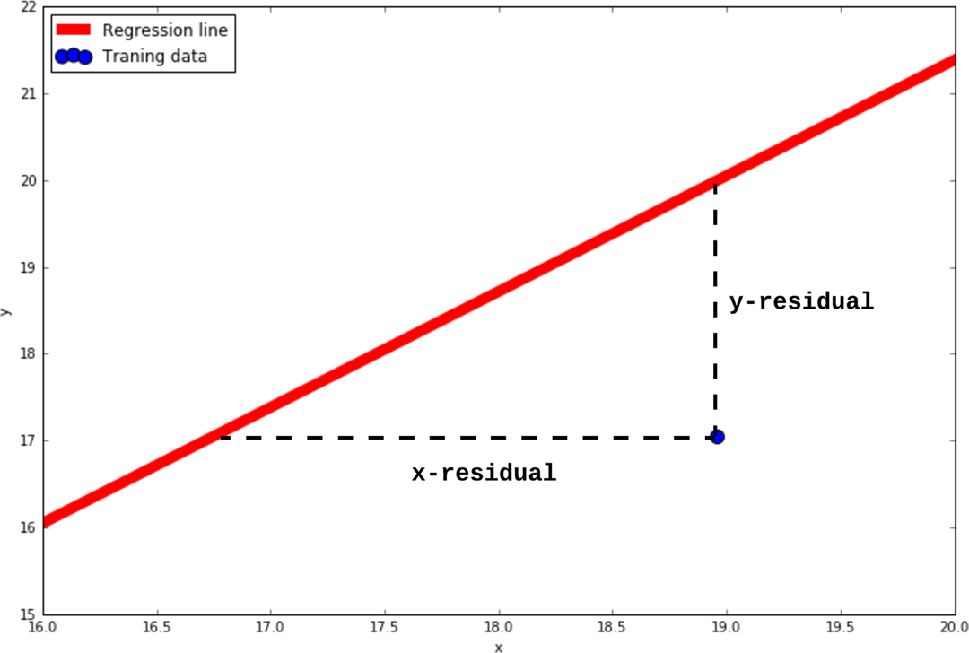
Figure A-1. Illustration of x- and y-residuals of a regression line for a single training data point

For gradient descent optimization algorithms, we need to find the gradient of this cost function by differentiating with respect to θ:

Now that you have some understanding of how the training of a regression model actually works, let’s try to implement our own version of scikit-learn’s fit() function. We begin by defining the logistic, cost, and gradient functions, as we just stated:

# Logistic function, also known as the sigmoid function
def logistic(x):
    return 1 / (1 + np.exp(-x))

# Logistic regression cost function
def cost(theta, X, y):
    X = X.values
    y = y.values

    # Note that we clip the minimum values to slightly above
    # zero to avoid throwing an error when logarithm is applied
    log_prob_zero = np.log(
        (1 - logistic(np.dot(X, theta))).clip(min=1e-10))
    log_prob_one = np.log(
        logistic(np.dot(X, theta)).clip(min=1e-10))

    # Calculate the log-likelihood terms
    zero_likelihood = (1 - y) * log_prob_zero
    one_likelihood = -y * log_prob_one

    # Sum across all the samples, then take the mean
    return np.sum(one_likelihood - zero_likelihood) / (len(X))


# Logistic regression gradient function
def gradient(theta, X, y):
    X = X.values
    y = y.values

    num_params = theta.shape[0]
    grad = np.zeros(num_params)
    err = logistic(np.dot(X, theta)) - y

    # Iterate through parameters and calculate
    # gradient for each given current error
    for i in range(num_params):
        term = np.multiply(err, X[:, i])
        grad[i] = np.sum(term) / len(X)

    return grad

Continuing from the payment fraud detection example in “Machine Learning in Practice: A Worked Example” (where the data has already been read and the training/test sets created), let’s further prepare the data for optimization. Note that we are trying to optimize eight model parameters. Having k + 1 model parameters, where k is the number of features in the training set (in this case, k = 7), is typical for logistic regression because we have a separate “weight” for each feature plus a “bias” term. For more convenient matrix multiplication shape-matching, we will insert a column of zeros into X:

# Insert column of zeros for more convenient matrix multiplication
X_train.insert(0, 'ones', 1)
X_test.insert(0, 'ones', 1)

Next, we randomly initialize our model parameters in a size-8 array and give it the name theta:

# Seed for reproducibility
np.random.seed(17)
theta = np.random.rand(8)

As a baseline, let’s evaluate the cost in the model’s current unoptimized state:

cost(theta, X_train, y_train)

> 20.38085906649756

Now, we use an implementation of the gradient descent algorithm provided by SciPy, scipy.optimize.fmin_tnc. The underlying optimization algorithm is the Newton Conjugate-Gradient method,¹ an optimized variant of the simple gradient descent that we described earlier (in scikit-learn, you can use this solver by specifying solver:'newton-cg'):

from scipy.optimize import fmin_tnc

res = fmin_tnc(func=cost, x0=theta, fprime=gradient,
               args=(X_train, y_train))

The results of the gradient descent optimization are stored in the res tuple object. Inspecting res (and consulting the function documentation), we see that the zeroth position in the tuple contains the solution (i.e., our eight trained model parameters), the first position contains the number of function evaluations, and the second position contains a return code:

> (array([ 19.25533094, −31.22002744,   0.55258124,   4.05403275,
           −3.85452354,  10.60442976,  10.39082921,  12.69257041]), 55, 0)

It looks like it took 55 iterations of the gradient descent algorithm to successfully reach the local minimum² (return code 0), and we have our optimized model parameters. Let’s see what the value of the cost function is now:

cost(res[0], X_train, y_train)

> 1.3380705016954436e-07

The optimization appears to have been quite successful, bringing down the cost from the initial value of 20.38 to the current value of 0.0000001338. Let’s evaluate these trained parameters on the test set and see how well the trained logistic regression model actually does. We first define a get_predictions() function, which simply does a matrix multiplication of the test data and theta before passing it into the logistic function to get a probability score:

def get_predictions(theta, X):
    return [1 if x >= 0.5 else 0 for x in logistic(X.values * theta.T)]

Then, let’s run a test by passing in the test data and comparing it to the test labels:

y_pred_new = get_predictions(np.matrix(res[0]), X_test)
print(accuracy_score(y_pred_new, y_test.values))

> 1.0

We achieved 100% accuracy on the test data! It seems like the optimization worked and we have successfully trained the logistic regression model.