Vladimir SilvaPractical Quantum Computing for Developershttps://doi.org/10.1007/978-1-4842-4218-6_7

7. Game Theory: With Quantum Mechanics, Odds Are Always in Your Favor

Vladimir Silva¹

(1)

CARY, NC, USA

This chapter explores two game puzzles that show the remarkable power of quantum algorithms over their classical counterparts:

The counterfeit coin puzzle: It is a classical balance puzzle proposed by mathematician E. D. Schell in 1945. It is about balancing coins to determine which holds a different value (counterfeit) using a balance scale and a limited number of tries.
The Mermin-Peres Magic Square game: This is an example of quantum pseudo-telepathy or the ability of players to achieve outcomes that would only be possible if they mysteriously communicate during the game.

In both cases, quantum computation gives quasi-magical abilities to the players, just as if they were cheating all along. Let’s see how.

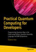
Counterfeit Coin Puzzle

In this puzzle, the player has eight coins and a beam balance. One of the coins is fake and thus underweight. The goal of the game is to figure out which coin is fake by using the balance only twice. Can you figure out how? Let’s run through the solution shown in Figure 7-1.

1.
Given eight coins, put coins 1-3 on the left side of the balance and 4-6 on the right side. Leave the last two coins 7 and 8 on the side and weight.
2.
If the balance leans right, the counterfeit is among 1-3 (left). Remember that the fake coin is lighter. Thus take out the last coin from the left (3) and weight again (for the second time).
- If the beam leans right, the counterfeit is 1. Stop.
- If the beam leans left, the counterfeit is 2. Stop.
- If the beam is balanced, the counterfeit is 3. Stop.
3.
If the balance leans left, the counterfeit is among 4-6. Take out the last coin (6) and weight again.
- If the beam leans right, the counterfeit is 4. Stop.
- If the beam leans left, the counterfeit is 5. Stop.
- If the beam is balanced, the counterfeit is 6. Stop.
4.
If the beam is balanced, the counterfeit is either 7 or 8. Put 7 and 8 in the balance and weight again.
- If the beam leans right, the counterfeit is 7. Stop.
- If the beam leans left, the counterfeit is 8. Stop.

../images/469026_1_En_7_Chapter/469026_1_En_7_Fig1_HTML.jpg — Figure 7-1
Counterfeit puzzle solution for eight coins

From the procedure in the previous section, a classical algorithm can be implemented independent of the total number of coins N and the number of counterfeit coins k. In general terms, the time complexity of the generalized counterfeit coin puzzle is given by

$O\left(k\log \left(N/k\right)\right)$

Tip

It has been proven that the minimal number of tries required to find a single counterfeit coin using the balance beam in a classical computer is two.

Counterfeit Coin, the Quantum Way

Believe it or not, there is a quantum algorithm that can find the counterfeit using a quantum balance only once, independent of the number of coins N! In general terms, for any number of counterfeit coins k, independent of N, the time complexity of such algorithm is given by

$O\left({k}^{1/4}\right)$

../images/469026_1_En_7_Chapter/469026_1_En_7_Fig2_HTML.jpg — Figure 7-2
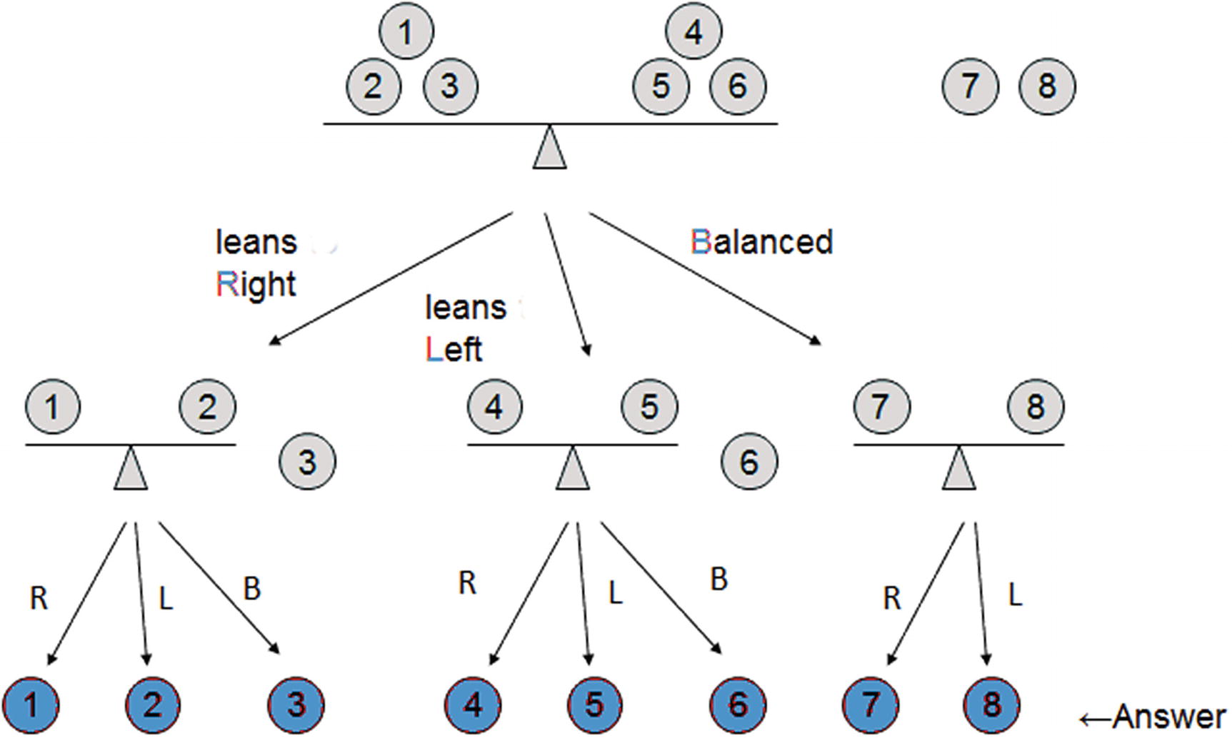
Quantum vs. classical time complexities for the counterfeit coin puzzle

Tip

The quantum counterfeit coin algorithm is an example of quartic speedup over its classical counterpart.

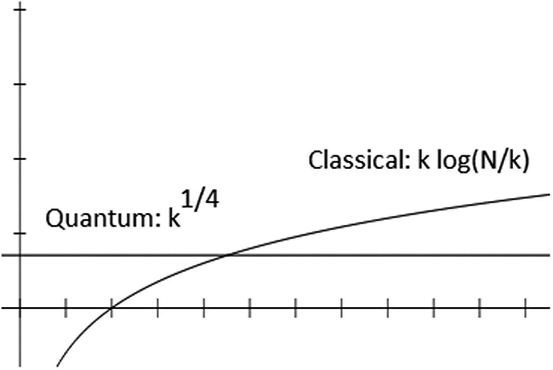
Thus Figure 7-2 shows the power of a quantum algorithm over its classical counterpart for the counterfeit coin puzzle. Now, let’s dig deeper. A quantum algorithm to find a single counterfeit coin (k = 1) can be summarized in three stages: query the quantum beam balance, construct the quantum balance, and identify the false coin.

Step 1: Query the Quantum Beam Balance

A quantum algorithm will query the beam balance in superposition. To do this, we use a binary query string to encode coins placed on the pans. For example, the query string 11101111 means all coins are on the beam except coin with index 3. The beam is balanced when no false coin is included and tilted otherwise. The next table illustrates this.

N (# of coins)	F (index of false coin)	Query string	Result
8	3	11101111	Balanced (0)
8	3	11111111	Tilted (1)

The procedure can be summarized as follows:

1.
Use two quantum registers to query the quantum balance, where the first register is for the query string and the second register for the result.
2.
Prepare the superposition of all binary query strings with even number of 1s.
3.
To obtain the superposition of states of even number of 1s, perform a Hadamard transform on the basis state |0>, and check if the Hamming weight of |x| is even. It can be shown that the Hamming weight of |x| is even if and only if x1 ⊕ x2 ⊕ … ⊕ xN = 0.

Tip

The Hamming weight (hw) of a string is the number of symbols that are different from the zero symbol of the alphabet used. For example, hw(11101) = 4, hw(11101000) = 4, hw(000000) = 0.

4.
Finally, measure the second register, and if |0> is observed, then the first register is the superposition of all binary query strings we want. If we get |1> then repeat the procedure until |0> is observed.

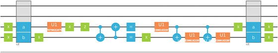
Note that each repetition is guaranteed to succeed with probability exactly half. Hence, after several repetitions, we should be able to obtain the desired superposition state. Listing 7-1 shows an implementation of a quantum program to query the beam balance with the corresponding graphical circuit shown in Figure 7-3.

Note

For the sake of clarity, the full counterfeit coin program has been broken in Listings 7-1 thru 7-3. Although you should be able to join the sections to run the program, a full listing is available from the source at Workspace\Ch07\p_counterfeitcoin.py.

# ------- Query the quantum beam balance

Q_program = QuantumProgram()

Q_program.set_api(Qconfig.APItoken, Qconfig.config["url"])

# Create numberOfCoins +1 quantum/classic registers

# 1 extra qubit for recording the result of quantum balance

qr = Q_program.create_quantum_register("qr", numberOfCoins +1 )

# for recording the measurement on qr

cr = Q_program.create_classical_register("cr", numberOfCoins + 1)

circuitName = "QueryStateCircuit"

circuit = Q_program.create_circuit(circuitName, [qr], [cr])

N = numberOfCoins

#Create uniform superposition of all strings of length N

for i in range(N):

circuit.h(qr[i])

#Perform XOR(x) by applying CNOT gates sequentially from qr[0] to qr[N-1]

# and storing the result to qr[N]

for i in range(N):

circuit.cx(qr[i], qr[N])

# Measure qr[N] and store the result to cr[N].

# continue if cr[N] is zero, or repeat otherwise

circuit.measure(qr[N], cr[N])

# query the quantum beam balance if the value of cr[0]...cr[N] is all 0

# by preparing the Hadamard state of |1>, i.e., |0> - |1> at qr[N]

circuit.x(qr[N]).c_if(cr, 0)

circuit.h(qr[N]).c_if(cr, 0)

# rewind the computation when cr[N] is not zero

for i in range(N):

circuit.h(qr[i]).c_if(cr, 2**N)

Listing 7-1

Script to Query the Quantum Beam Balance

Figure 7-3 shows a complete circuit for counterfeit coin puzzle for eight coins, one counterfeit at index 6. The circuit displays all the stages described here for the IBM Q Experience platform. The second stage in the algorithm is to construct the beam balance.

../images/469026_1_En_7_Chapter/469026_1_En_7_Fig3_HTML.jpg — Figure 7-3
Quantum circuit for the counterfeit coin puzzle with N = 8, k = 1, and fake at index 6 (Note: For full-size viewing, this graph is included in the source code download)

Step 2: Construct the Quantum Balance

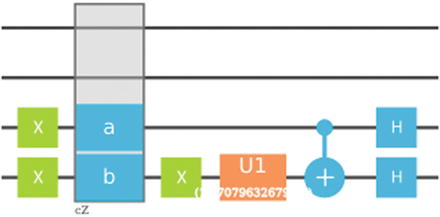
In the previous section, we constructed the superposition of all binary query strings whose Hamming weights are even. In this step, we construct the quantum beam by setting the position of the false coin. Thus given k is the position of the false coin with regard to the binary string |x1, x2, …, xN>|0>, the quantum beam balance returns

|x1, x2, … , xN> |0⊕xk>

This is implemented with a CNOT gate with xk as the control and the second register as the target (see partial Listing 7-2).

#----- Construct the quantum beam balance

k = indexOfFalseCoin

# Apply the quantum beam balance on the desired superposition state

#(marked by cr equal to zero)

circuit.cx(qr[k], qr[N]).c_if(cr, 0)

Listing 7-2

Construct the Quantum Beam Balance

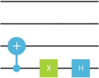
Step 3: Identify the False Coin

To identify the false coin after querying the balance, apply a Hadamard transform on the binary query string. Assuming that we query the quantum beam balance with binary strings of even Hamming weight, then by performing the measurement in the computational basis after the Hadamard transform, we can identify the false coin because it is the one whose label is different from the majority (see Listing 7-3).

# --- Identify the false coin

# Apply Hadamard transform on qr[0] ... qr[N-1]

for i in range(N):

circuit.h(qr[i]).c_if(cr, 0)

# Measure qr[0] ... qr[N-1]

for i in range(N):

circuit.measure(qr[i], cr[i])

results = Q_program.execute([circuitName], backend=backend, shots=shots)

answer = results.get_counts(circuitName)

print("Device " + backend + " counts " + str(answer))

# Get most common label

for key in answer.keys():

normalFlag, _ = Counter(key[1:]).most_common(1)[0]

for i in range(2,len(key)):

if key[i] != normalFlag:

print("False coin index is: ", len(key) - i - 1)

Listing 7-3

Identify the False Coin

When the leftmost bit is 0, the index of the false coin can be determined by finding the one whose values are different from others. For example, for N = 8, false index = 6, then the result should be 010111111 or 001000000. Note that because we use cr[N] to control the operation prior to and after the query to the balance, then

If the leftmost bit is 0, then we succeed in identifying the false coin.
If the leftmost bit is 1, we failed to obtain the desired superposition and must repeat the process from the beginning.

Running the program against the remote IBM Q Experience simulator gives the result (under book source Workspace\Ch07\p_counterfeitcoin.py). Note that I am using Windows in this instance:

c:\python36-64\python.exe p_counterfeitcoin.py

Device ibmq_qasm_simulator counts {'001000000': 1}

False coin index is: 6

If you don’t have access to the book source and still want to play with this script, paste the snippets in the previous sections inside the container script in Listing 7-4 (watch out for Python’s indentation idiosyncrasies; they will drive you nuts).

import sys

import matplotlib.pyplot as plt

import numpy as np

from math import pi, cos, acos, sqrt

from collections import Counter

from qiskit import QuantumProgram

sys.path.append('../Config/')

import Qconfig

# import basic plot tools

from qiskit.tools.visualization import plot_histogram

def main(M = 16, numberOfCoins = 8 , indexOfFalseCoin = 6

, backend = "local_qasm_simulator" , shots = 1 ):

if numberOfCoins < 4 or numberOfCoins >= M:

raise Exception("Please use numberOfCoins between 4 and ", M-1)

if indexOfFalseCoin < 0 or indexOfFalseCoin >= numberOfCoins:

raise Exception("indexOfFalseCoin must be between 0 and ", numberOfCoins-1)

// Paste listings 7-1 -> 7-3 here

#################################################

# main

#################################################

if __name__ == '__main__':

M = 8 #Maximum qubits available

numberOfCoins = 4 #Up to M-1, where M is the number of qubits available

indexOfFalseCoin = 2 #This should be 0, 1, ..., numberOfCoins - 1,

backend = "ibmq_qasm_simulator"

#backend = "ibmqx3"

shots = 1 # We perform a one-shot experiment

main(M, numberOfCoins, indexOfFalseCoin, backend, shots)

Listing 7-4

Counterfeit Coin Puzzle Main Container Script

Generalization for Any Number of False Coins

The counterfeit coin puzzle has been generalized by any number of fake coins (k>1) by mathematicians Terhal and Smolin in 1998. Their implementation uses a Balance Oracle model (B-Oracle) such that

Given an input of N bits x = x1x2…xn Є {0, 1}^N.
Construct a query string of N tri-bits such that q = q1q2…qn ∈ {0, 1, −1}^N with the same number of 1s and -1s.
The answer is 1 bit such that $\chi \left(x;q\right)=\Big\{{\displaystyle \begin{array}{c}0\kern0.28em if\kern0.28em q1x1+q2x2+\dots qnxn=0\kern0.28em (balanced)\kern1.75em \\ {}1\kern0.28em otherwise\kern8em (tilted)\kern3.25em \end{array}}$ .

Tip

An Oracle is the portion of an algorithm regarded as a black box. It is used to simplify circuits and provide complexity comparisons between quantum and classical algorithms. A good Oracle should provide speed, generality, and feasibility.

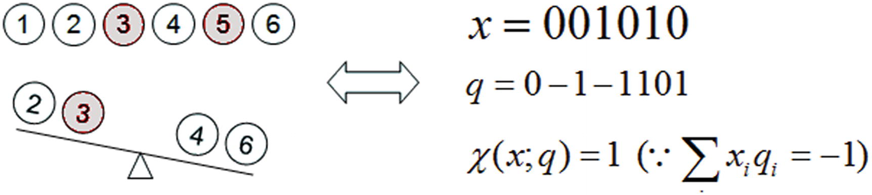
An example of the B-Oracle in action is shown in Figure 7-4 for two fake coins: k = 2 and N = 6.

../images/469026_1_En_7_Chapter/469026_1_En_7_Fig4_HTML.jpg — Figure 7-4
B-Oracle for N = 6 and k = 2 )

All in all, the counterfeit puzzle is the quintessential example of quartic speedup of a quantum algorithm over its classical counterpart. In the next section, we look at another bizarre quasi-magical puzzle called the Mermin-Peres Magic Square.

Mermin-Peres Magic Square

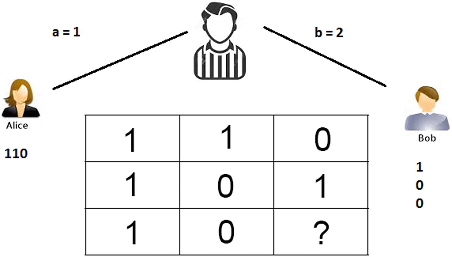
This is another classic puzzle first proposed by physicists David Mermin and A. Peres as an example of quantum pseudo-telepathy or the ability of two players to have some supernatural communication to outside observers. Thanks to the magic of entanglement, this is possible. Let’s take a closer look.

../images/469026_1_En_7_Chapter/469026_1_En_7_Fig5_HTML.jpg — Figure 7-5
Mermin-Peres Magic Square

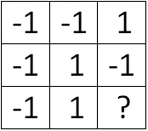
The game starts with two players Alice and Bob against a referee. The magic square is a 3x3 matrix with the following rules (see Figure 7-5):

All entries are either 0 or 1 such that the sum of entries on each row is even, and the sum of each column is odd. The game is called the magic square because such square is impossible; as shown in Figure 7-5, there is no valid combination where the sum of rows is even and the sum of columns is odd (try it yourself with pen and paper). This is due to the odd number of entries in the matrix.
The referee sends an integer a Є {1,2,3} to Alice and another b Є {1,2,3} to Bob. Alice must reply with the a-th row of the square. Bob must reply with the b-th column.
Alice and Bob win if the sum of Alice’s entries is even, the sum of Bob’s is odd, and their intersecting answer is the same. Otherwise, the referee wins.
Prior to the start, Alice and Bob can strategize and share information. For example, they could decide to answer using the matrix in Figure 7-5. However they are not allowed to communicate during the game.

For example, in the preceding matrix, if the referee sends a = 1 to Alice and b = 2 to Bob, Alice would reply with 110 (row 1) and Bob with 100 (column 2). The element in the intersection of the answers (row 1-column 2) is the same (1) so they win the game. It can be shown that in a classical setting, the winning probability for Alice and Bob is at most 8/9. That is, there are eight out of nine permutations in the square for victory. Therefore Alice and Bob’s winning probability is at most 88.8%.

Let’s put this assertion to the test with a neat exercise to prove that indeed the classical winning probability for the magic square is at most 8/9 (88.88%).

Mermin-Peres Magic Square Exercise

1.
Construct a magic square similar to Figure 7-5 using the binary code (1, -1) instead of (1, 0) where the product of the row elements is 1 (even), and the product of the column elements is -1 (odd). Confirm that in fact this is not possible.
2.
Create a permutation table for the referee values for a and b using the square in step 1 including
- A permutation count number.
- The values for a, b.
- Alice and Bob’s response.
- The intersection of Alice and Bob’s response. Remember that it must be equal for them to win.
- The result of the game iteration: Win = W, Loose = L.
3.
Finally calculate the winning probability and prove that it is at most 8/9. Note: Answers are at the end of the section .

Quantum Winning Strategy

Thanks to the power of quantum mechanics and the magic of entanglement, Alice and Bob can do much better. In fact they can win the game 100% of the time, as if they were communicating telepathically, hence the term pseudo-telepathy. A quantum winning strategy was first proposed by Brassard and colleagues¹ and it is divided in three stages:

Shared entangled state: This is the key for Alice and Bob to win 100% of the time.
Unitary transformations for Alice and Bob’s inputs: These provide the responses to be sent back to the referee.
Measure in the computational basis: The final stage to construct a final response.

Shared Entangled State

In the quantum winning strategy, Alice and Bob share the entangled state:

$\varPsi =\frac{1}{2}\mid 0011\left\rangle -\frac{1}{2}\mid 0110\right\rangle -\frac{1}{2}\mid 1001\left\rangle +\frac{1}{2}\mid 1100\right\rangle$

A circuit implementation requires 2 qubits for Alice and 2 for Bob as shown in Figure 7-6.

../images/469026_1_En_7_Chapter/469026_1_En_7_Fig6_HTML.jpg — Figure 7-6
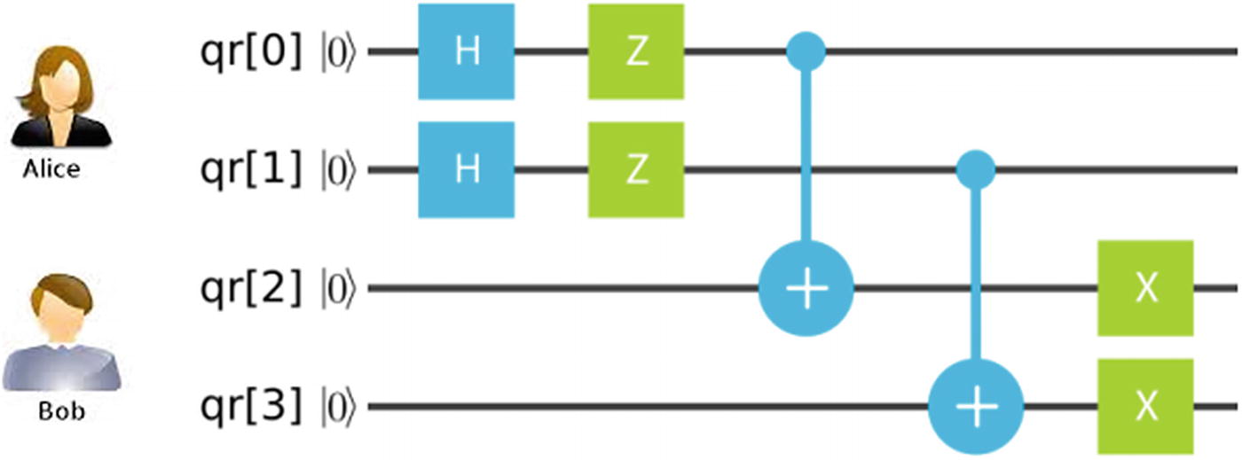
Entangled state for the magic square

We know that the Hadamard maps the basis state $H\mid 0\Big\rangle \to \frac{1}{\sqrt{2}}\left(\left|0\Big\rangle +|1\right\rangle \right)$ . Thus applying for the first 2 qubits yields $\varPsi =\frac{1}{2}\mid 00\left\rangle +\frac{1}{2}\mid 01\right\rangle +\frac{1}{2}\mid 10\left\rangle +\frac{1}{2}\mid 11\right\rangle$ .
Next apply a Z gate to the first 2 qubits. Remember that Z leaves the 0 state unchanged and maps 1 to -1 (flipping the sign of the preceding third term). At this stage the state becomes $\varPsi =\frac{1}{2}\mid 00\left\rangle +\frac{1}{2}\mid 01\right\rangle -\frac{1}{2}\mid 10\left\rangle +\frac{1}{2}\mid 11\right\rangle$ .
Next apply the CNOT gate to entangle qubits 0-2 and 1-3: $\varPsi =\frac{1}{2}\mid 0000\left\rangle -\frac{1}{2}\left\langle 0101|-\frac{1}{2}|1010\right\rangle +\frac{1}{2}\mid 1111\right\rangle$ .
Finally flip the last 2 qubits with the X gate for $\varPsi =\frac{1}{2}\mid 0011\left\rangle -\frac{1}{2}\mid 0110\right\rangle -\frac{1}{2}\mid 1001\left\rangle +\frac{1}{2}\mid 1100\right\rangle$ .

The Python script to construct the entangled state is given in Listing 7-5.

# Create the entangle state

Q_program = QuantumProgram()

Q_program.set_api(Qconfig.APItoken, Qconfig.config["url"])

# 4 qubits (Alice = 2, Bob = 2)

N = 4

# Creating registers

qr = Q_program.create_quantum_register("qr", N)

# for recording the measurement on qr

cr = Q_program.create_classical_register("cr", N)

circuitName = "sharedEntangled"

sharedEntangled = Q_program.create_circuit(circuitName, [qr], [cr])

#Create uniform superposition of all strings of length 2

for i in range(2):

sharedEntangled.h(qr[i])

#The amplitude is minus if there are odd number of 1s

for i in range(2):

sharedEntangled.z(qr[i])

#Copy the content of the first two qubits to the last two qubits

for i in range(2):

sharedEntangled.cx(qr[i], qr[i+2])

#Flip the last two qubits

for i in range(2,4):

sharedEntangled.x(qr[i])

Listing 7-5

Quantum Winning Strategy Entangled State

With the shared entangled state, Alice and Bob can now start the game and receive their inputs from the referee.

Unitary Transformations

Upon receiving their inputs a Є {1,2,3} and b Є {1,2,3}, Alice and Bob apply the following unitary transformations: A1, A2, A3 for Alice and B1, B2, B3 for Bob to the shared entangled states:

$A1=\frac{1}{\sqrt{2}}\left[\begin{array}{cccc}i& 0& 0& 1\\ {}0& -i& 1& 0\\ {}0& i& 1& 0\\ {}1& 0& 0& i\end{array}\right],A2=\frac{1}{2}\left[\begin{array}{cccc}i& 1& 1& i\\ {}-i& 1& -1& i\\ {}i& 1& 1& -i\\ {}-i& 1& -1& -i\end{array}\right],A3=\frac{1}{2}\left[\begin{array}{cccc}-1& -1& -1& 1\\ {}1& 1& -1& 1\\ {}1& -1& 1& 1\\ {}1& -1& -1& -1\end{array}\right]$

$B1=\frac{1}{2}\left[\begin{array}{cccc}i& -i& 1& 1\\ {}-i& -i& 1& -1\\ {}1& 1& -i& i\\ {}-i& i& 1& 1\end{array}\right],B2=\frac{1}{2}\left[\begin{array}{cccc}-1& i& 1& i\\ {}1& i& 1& -i\\ {}1& -i& 1& i\\ {}-1& -i& 1& -i\end{array}\right],B3=\frac{1}{\sqrt{2}}\left[\begin{array}{cccc}1& 0& 0& 1\\ {}-1& 0& 0& 1\\ {}0& 1& 1& 0\\ {}0& 1& -1& 0\end{array}\right]$

Note

Remember that by applying the preceding transformations to their entangled states, Alice and Bob are able to construct the first 2 bits of their respective responses to the referee.

Listing 7-6 shows the unitary transformations for Alice and Bob with equivalent graphical circuits in Table 7-1.

#------ circuits of Alice's and Bob's operations.

#we first define controlled-u gates required to assign phases

from math import pi

def ch(qProg, a, b):

""" Controlled-Hadamard gate """

qProg.h(b)

qProg.sdg(b)

qProg.cx(a, b)

qProg.h(b)

qProg.t(b)

qProg.cx(a, b)

qProg.t(b)

qProg.h(b)

qProg.s(b)

qProg.x(b)

qProg.s(a)

return qProg

def cu1pi2(qProg, c, t):

""" Controlled-u1(phi/2) gate """

qProg.u1(pi/4.0, c)

qProg.cx(c, t)

qProg.u1(-pi/4.0, t)

qProg.cx(c, t)

qProg.u1(pi/4.0, t)

return qProg

def cu3pi2(qProg, c, t):

""" Controlled-u3(pi/2, -pi/2, pi/2) gate """

qProg.u1(pi/2.0, t)

qProg.cx(c, t)

qProg.u3(-pi/4.0, 0, 0, t)

qProg.cx(c, t)

qProg.u3(pi/4.0, -pi/2.0, 0, t)

return qProg

#----------------------------------------------------------------------

# Define circuits used by Alice and Bob for each of their inputs: 1,2,3

# dictionary for Alice's operations/circuits

aliceCircuits = {}

# Quantum circuits for Alice 1, 2, 3

for idx in range(1, 4):

circuitName = "Alice"+str(idx)

aliceCircuits[circuitName]

= Q_program.create_circuit(circuitName, [qr], [cr])

theCircuit = aliceCircuits[circuitName]

if idx == 1:

#the circuit of A_1

theCircuit.x(qr[1])

theCircuit.cx(qr[1], qr[0])

theCircuit = cu1pi2(theCircuit, qr[1], qr[0])

theCircuit.x(qr[0])

theCircuit.x(qr[1])

theCircuit = cu1pi2(theCircuit, qr[0], qr[1])

theCircuit.x(qr[0])

theCircuit = cu1pi2(theCircuit, qr[0], qr[1])

theCircuit = cu3pi2(theCircuit, qr[0], qr[1])

theCircuit.x(qr[0])

theCircuit = ch(theCircuit, qr[0], qr[1])

theCircuit.x(qr[0])

theCircuit.x(qr[1])

theCircuit.cx(qr[1], qr[0])

theCircuit.x(qr[1])

elif idx == 2:

theCircuit.x(qr[0])

theCircuit.x(qr[1])

theCircuit = cu1pi2(theCircuit, qr[0], qr[1])

theCircuit.x(qr[0])

theCircuit.x(qr[1])

theCircuit = cu1pi2(theCircuit, qr[0], qr[1])

theCircuit.x(qr[0])

theCircuit.h(qr[0])

theCircuit.h(qr[1])

elif idx == 3:

theCircuit.cz(qr[0], qr[1])

theCircuit.swap(qr[0], qr[1]) # not supported in composer

theCircuit.h(qr[0])

theCircuit.h(qr[1])

theCircuit.x(qr[0])

theCircuit.x(qr[1])

theCircuit.cz(qr[0], qr[1])

theCircuit.x(qr[0])

theCircuit.x(qr[1])

#measure the first two qubits in the computational basis

theCircuit.measure(qr[0], cr[0])

theCircuit.measure(qr[1], cr[1])

# dictionary for Bob's operations/circuits

bobCircuits = {}

# Quantum circuits for Bob when receiving 1, 2, 3

for idx in range(1,4):

circuitName = "Bob"+str(idx)

bobCircuits[circuitName]

= Q_program.create_circuit(circuitName, [qr], [cr])

theCircuit = bobCircuits[circuitName]

if idx == 1:

theCircuit.x(qr[2])

theCircuit.x(qr[3])

theCircuit.cz(qr[2], qr[3])

theCircuit.x(qr[3])

theCircuit.u1(pi/2.0, qr[2])

theCircuit.x(qr[2])

theCircuit.z(qr[2])

theCircuit.cx(qr[2], qr[3])

theCircuit.cx(qr[3], qr[2])

theCircuit.h(qr[2])

theCircuit.h(qr[3])

theCircuit.x(qr[3])

theCircuit = cu1pi2(theCircuit, qr[2], qr[3])

theCircuit.x(qr[2])

theCircuit.cz(qr[2], qr[3])

theCircuit.x(qr[2])

theCircuit.x(qr[3])

elif idx == 2:

theCircuit.x(qr[2])

theCircuit.x(qr[3])

theCircuit.cz(qr[2], qr[3])

theCircuit.x(qr[3])

theCircuit.u1(pi/2.0, qr[3])

theCircuit.cx(qr[2], qr[3])

theCircuit.h(qr[2])

theCircuit.h(qr[3])

elif idx == 3:

theCircuit.cx(qr[3], qr[2])

theCircuit.x(qr[3])

theCircuit.h(qr[3])

#measure the third and fourth qubits in the computational basis

theCircuit.measure(qr[2], cr[2])

theCircuit.measure(qr[3], cr[3])

Listing 7-6

Unitary Transformations for Alice and Bob

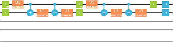
Table 7-1 shows quantum circuits for the unitary transformations A1-3, B1-3 for IBM Q Experience Composer.

Table 7-1

Quantum Circuits for the Unitary Transformations in Listing 7-6

Transformation	Circuit
$A1=\frac{1}{\sqrt{2}}\left[\begin{array}{cccc}i& 0& 0& 1\\ {}0& -i& 1& 0\\ {}0& i& 1& 0\\ {}1& 0& 0& i\end{array}\right]$
$A2=\frac{1}{2}\left[\begin{array}{cccc}i& 1& 1& i\\ {}-i& 1& -1& i\\ {}i& 1& 1& -i\\ {}-i& 1& -1& -i\end{array}\right]$
$B1=\frac{1}{2}\left[\begin{array}{cccc}i& -i& 1& 1\\ {}-i& -i& 1& -1\\ {}1& 1& -i& i\\ {}-i& i& 1& 1\end{array}\right]$
$B2=\frac{1}{2}\left[\begin{array}{cccc}-1& i& 1& i\\ {}1& i& 1& -i\\ {}1& -i& 1& i\\ {}-1& -i& 1& -i\end{array}\right]$
$B3=\frac{1}{\sqrt{2}}\left[\begin{array}{cccc}1& 0& 0& 1\\ {}-1& 0& 0& 1\\ {}0& 1& 1& 0\\ {}0& 1& -1& 0\end{array}\right]$

In Table 7-1 note that A3 is not included due to the fact that the Composer does not support the swap gate required by Listing 7-6. This does not mean the quantum program can’t be run in the simulator or real device however. It simply means the circuit cannot be created in the Composer. Thus for the final step, Alice and Bob measure their qubits in the computational basis .

Measure in the Computational Basis

After measurement, Alice and Bob end up with 2 bits each which represent their respective outputs. To obtain the third bit, and thus a final answer, they apply their parity rules. That is, Alice’s sum must be even, and Bob’s must be odd. For example, for a = 2, b = 3 (see Table 7-2)

$\begin{array}{l}\left(A2\otimes B3\right)\mid \psi \left\rangle =\frac{1}{2\sqrt{2}}\right[\mid 0000\left\rangle -\mid 0010\right\rangle -\mid 0101\left\rangle +\mid 0111\right\rangle +\mid 1001\Big\rangle \\ {}\kern7.25em -\mid 1011\left\rangle -\mid 1100\right\rangle -\mid 1110\Big\rangle \end{array}$

Table 7-2

Answer Permutations for a = 2, b =3 of the Magic Square

ψ	Alice’s answer	Bob’s answer	Square
\|0000>	000	001	$\left[0\kern0.375em 0\kern0.375em \begin{array}{l}0\\ {}0\\ {}1\end{array}\right]$
\|0010>	000	100	$\left[0\kern0.5em 0\kern0.5em \begin{array}{l}1\\ {}0\\ {}0\end{array}\right]$
\|0101>	011	010	$\left[0\kern0.5em 1\kern0.5em \begin{array}{l}1\\ {}1\\ {}0\end{array}\right]$
\|0111>	011	111	$\left[0\kern0.5em 1\kern0.5em \begin{array}{l}1\\ {}1\\ {}1\end{array}\right]$
\|1001>	101	010	$\left[1\kern0.5em 0\kern0.5em \begin{array}{l}0\\ {}1\\ {}0\end{array}\right]$
\|1011>	101	111	$\left[1\kern0.5em 0\kern0.5em \begin{array}{l}1\\ {}1\\ {}1\end{array}\right]$
\|1100>	110	001	$\left[1\kern0.5em 1\kern0.5em \begin{array}{l}0\\ {}0\\ {}1\end{array}\right]$
\|1110>	110	101	$\left[1\kern0.5em 1\kern0.5em \begin{array}{l}1\\ {}0\\ {}1\end{array}\right]$

Listing 7-7 shows a section of the script to loop through all the rounds of the magic square:

It loops through a[1,3] and b[1,3] inclusive.
For each (a, b), a circuit for Alice (Alice-a) and a circuit for Bob (Bob-b) are retrieved from Listing 7-6.
The shared entangled state ψ and Alice-a and Bob-b circuits are submitted for execution to the simulator or real quantum device.
Two bits are extracted for Alice and two for Bob from the answer such as {‘0011’: 1}.
The parity rules are applied: Alice’s sum must be even, and Bob’s sum must be odd.
Finally the answer is verified, and the winning probability is displayed.

def all_rounds(backend, real_dev, shots=10):

nWins = 0

nLost = 0

for a in range(1,4):

for b in range(1,4):

print("Asking Alice and Bob with a and b are: ", a,b)

rWins = 0

rLost = 0

aliceCircuit = aliceCircuits["Alice" + str(a)]

bobCircuit = bobCircuits["Bob" + str(b)]

circuitName = "Alice" + str(a) + "Bob"+str(b)

Q_program.add_circuit(circuitName, sharedEntangled+aliceCircuit+bobCircuit)

if real_dev:

ibmqx2_backend = Q_program.get_backend_configuration(backend)

ibmqx2_coupling = ibmqx2_backend['coupling_map']

results = Q_program.execute([circuitName], backend=backend, shots=shots

, coupling_map=ibmqx2_coupling, max_credits=3, wait=10, timeout=240)

else:

results = Q_program.execute([circuitName], backend=backend, shots=shots)

answer = results.get_counts(circuitName)

for key in answer.keys():

kfreq = answer[key] #frequencies of keys obtained from measurements

aliceAnswer = [int(key[-1]), int(key[-2])]

bobAnswer = [int(key[-3]), int(key[-4])]

if sum(aliceAnswer) % 2 == 0:

aliceAnswer.append(0)

else:

aliceAnswer.append(1)

if sum(bobAnswer) % 2 == 1:

bobAnswer.append(0)

else:

bobAnswer.append(1)

if(aliceAnswer[b-1] != bobAnswer[a-1]):

#print(a, b, "Alice and Bob lost")

nLost += kfreq

rLost += kfreq

else:

#print(a, b, "Alice and Bob won")

nWins += kfreq

rWins += kfreq

print("\t#wins = ", rWins, "out of ", shots, "shots")

print("Number of Games = ", nWins+nLost)

print("Number of Wins = ", nWins)

print("Winning probabilities = ", (nWins*100.0)/(nWins+nLost))

#################################################

# main

#################################################

if __name__ == '__main__':

backend = "ibmq_qasm_simulator"

#backend = "ibmqx2"

real_dev = False

all_rounds(backend, real_dev)

Listing 7-7

Script for All Rounds of the Magic Square

A run of Listing 7-7 against the IBM Q Experience remote simulator is shown in Listing 7-8.

c:\python36-64\python.exe p_magicsq.py

For a = 1 , b = 1

ibmq_qasm_simulator answer: 1000 Alice: [0, 0, 0] Bob:[0, 1, 0]

ibmq_qasm_simulator answer: 1010 Alice: [0, 1, 1] Bob:[0, 1, 0]

ibmq_qasm_simulator answer: 1111 Alice: [1, 1, 0] Bob:[1, 1, 1]

ibmq_qasm_simulator answer: 0111 Alice: [1, 1, 0] Bob:[1, 0, 0]

ibmq_qasm_simulator answer: 0000 Alice: [0, 0, 0] Bob:[0, 0, 1]

ibmq_qasm_simulator answer: 0101 Alice: [1, 0, 1] Bob:[1, 0, 0]

#wins = 10 out of 10 shots

For a = 1 , b = 2

ibmq_qasm_simulator answer: 1000 Alice: [0, 0, 0] Bob:[0, 1, 0]

ibmq_qasm_simulator answer: 1001 Alice: [1, 0, 1] Bob:[0, 1, 0]

ibmq_qasm_simulator answer: 1111 Alice: [1, 1, 0] Bob:[1, 1, 1]

ibmq_qasm_simulator answer: 0110 Alice: [0, 1, 1] Bob:[1, 0, 0]

ibmq_qasm_simulator answer: 0000 Alice: [0, 0, 0] Bob:[0, 0, 1]

ibmq_qasm_simulator answer: 0001 Alice: [1, 0, 1] Bob:[0, 0, 1]

#wins = 10 out of 10 shots

...

For a = 3 , b = 3

ibmq_qasm_simulator answer: 1000 Alice: [0, 0, 0] Bob:[0, 1, 0]

ibmq_qasm_simulator answer: 1011 Alice: [1, 1, 0] Bob:[0, 1, 0]

ibmq_qasm_simulator answer: 1101 Alice: [1, 0, 1] Bob:[1, 1, 1]

ibmq_qasm_simulator answer: 1110 Alice: [0, 1, 1] Bob:[1, 1, 1]

ibmq_qasm_simulator answer: 0111 Alice: [1, 1, 0] Bob:[1, 0, 0]

ibmq_qasm_simulator answer: 0010 Alice: [0, 1, 1] Bob:[0, 0, 1]

#wins = 10 out of 10 shots

Number of Games = 90

Number of Wins = 90

Winning probability = 100.0

Listing 7-8

Simplified Standard Output from a Run of All Rounds of the Magic Square

Note

If running in a real device, the winning probability will not be 100% due to environmental noise and gate error.

Answers for the Mermin-Peres Magic Square Exercise

1.
A magic square whose row product is even and whose column product is odd is given in the following presentation. Note that such square is not possible due to the odd number of cells.

../images/469026_1_En_7_Chapter/469026_1_En_7_Figf_HTML.jpg

2.
The permutation table for the square in answer 1 is

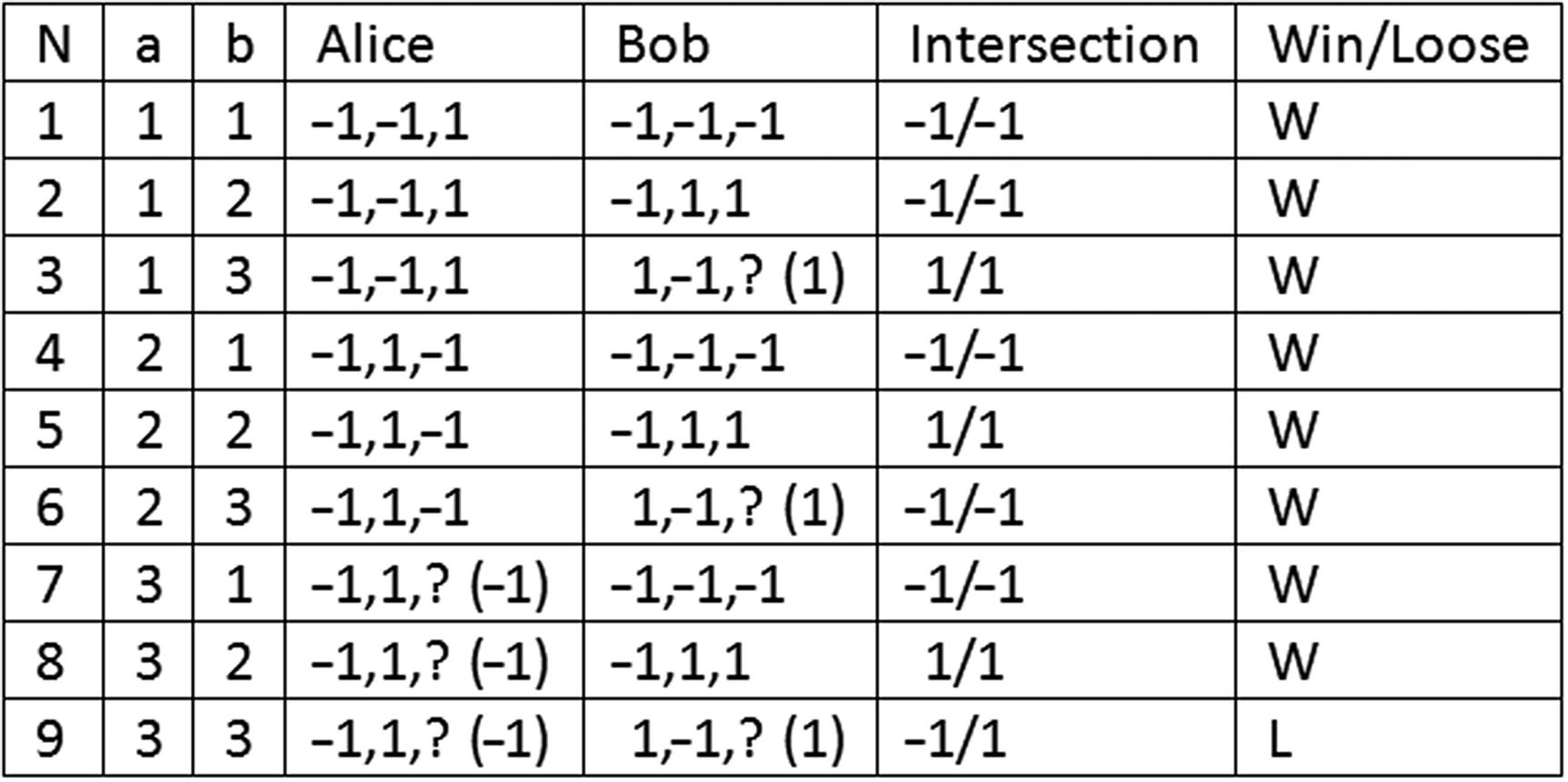
../images/469026_1_En_7_Chapter/469026_1_En_7_Figg_HTML.jpg

3.
Note that, in the previous step rows 7-9, Alice’s answer must be -1 so the product can be even (1). Plus, in columns 3, 6, and 9, Bob’s answer must be 1 so his product can be odd (−1). Finally, the probability is calculated by dividing the total number of wins by the total number of permutations. Thus

$P=\frac{\sum W}{N}=\frac{8}{9}=88.88\%$

In this chapter you have learned how the power of quantum entanglement can provide significant speedups over classical computation. With a quantum beam balance, it is possible to achieve quartic speedups for classical puzzles like the counterfeit coin problem. For others, such as the magic square, entanglement gives a quasi-magical telepathy among players. Now, if only Brassard and colleagues could come up with a quantum winning strategy for Black Jack or Poker, we will all be making a killing in Vegas right now. All in all, this chapter has shown how quantum mechanics is as confusing, bizarre, and fascinating as always. It never fails to deliver.

In the next and final chapter, you will learn about arguably the most famous quantum algorithm of them all: the notorious Shor’s integer factorization. An algorithm that may crumble asymmetric cryptography!

Previous Chapter

6. Fun with Quantum Games

Next Chapter

8. Faster Search plus Threatening the Foundation of Asymmetric Cryptography with Grover and Shor

Table of Contents for Practical Quantum Computing for Developers: Programming Quantum Rigs in the Cloud using Python, Quantum Assembly Language and IBM QExperience

7. Game Theory: With Quantum Mechanics, Odds Are Always in Your Favor

Counterfeit Coin Puzzle

Tip

Counterfeit Coin, the Quantum Way

Tip

Step 1: Query the Quantum Beam Balance

Tip

Note

Step 2: Construct the Quantum Balance

Step 3: Identify the False Coin

Generalization for Any Number of False Coins

Tip

Mermin-Peres Magic Square

Mermin-Peres Magic Square Exercise

Quantum Winning Strategy

Shared Entangled State

Unitary Transformations

Note

Measure in the Computational Basis

Note

Answers for the Mermin-Peres Magic Square Exercise

Table of Contents for
Practical Quantum Computing for Developers: Programming Quantum Rigs in the Cloud using Python, Quantum Assembly Language and IBM QExperience