Vladimir SilvaPractical Quantum Computing for Developershttps://doi.org/10.1007/978-1-4842-4218-6_4

4. QISKit, Awesome SDK for Quantum Programming in Python

Vladimir Silva¹

(1)

CARY, NC, USA

In this chapter you will get started with the QISKit, the best SDK out there for quantum programming. You will learn how easy it is to install the SDK in your local system. But before writing your first quantum program, it is always helpful to understand what quantum computation is and how it differs from classical computation. For this purpose, a very basic explanation of qubit states and quantum gates is presented using linear algebra. This section also shows how quantum computation can mirror its classical counterpart and furthermore find shortcuts to get results faster. Next, the chapter walks through the anatomy of a quantum program including system calls, circuit compilation formats, quantum assembly, and more.

QISKit packs a set of helpful simulators to execute your programs locally or remotely, but it also allows you to run in the real thing. Step by step, you will learn how to run your quantum programs in a real device provided by the awesome IBM Q Experience cloud platform. So start your desktop and let’s get to it.

Installing the QISKit

QISKit is the Quantum Information Software Kit, the de facto SDK for quantum programming in the cloud. It is written in Python, a powerful scripting language for scientific computing. My background has been mostly in business so I haven’t written much Python code over the years, so let’s see how the SDK can be installed both in Linux CentOS 6–7 and in Windows 64. We’ll begin with the easiest (Windows) and then jump to the trickiest (CentOS).

Setting Up in Windows

QISKit requires Python 3.5 or later. If you have a Windows system, chances are that you don’t have Python installed. If so, you can get the installers from the Python.org web site. Download the installer, run it, and verify your installation by running the following from the command window:

C:\>Python -V

Python 2.7.6

I have good old Python 2.7, yet you can have multiple versions of Python installed at the same time. In my case I downloaded the embeddable zip file and deployed to C:\Python36-64 so in my case:

C:\>C:\Python36-64\Python.exe -V

Python 3.6.4

Python features an amazing package manager called pip (preferred installer program) which makes installing modules very easy. Thus, to install QISKit, simply type at the console:

C:\>pip install qiskit

Your screen output should look similar to Listing 4-1. Make sure there are no error messages.

Collecting qiskit

Using cached qiskit-0.4.11.tar.gz

Collecting IBMQuantumExperience>=1.8.28 (from qiskit)

Using cached IBMQuantumExperience-1.9.0-py3-none-any.whl

Collecting matplotlib<2.2,>=2.1 (from qiskit)

Using cached matplotlib-2.1.2.tar.gz

Collecting networkx<2.1,>=2.0 (from qiskit)

Downloading networkx-2.0.zip (1.5MB)

100% |████████████████████| 1.6MB 400kB/s

Collecting numpy<1.15,>=1.13 (from qiskit)

Downloading numpy-1.14.2-cp36-cp36m-manylinux1_i686.whl (8.7MB)

100% |████████████████████| 8.7MB 105kB/s

...

Running setup.py install for pycparser ... done

Running setup.py install for matplotlib ... done

Running setup.py install for networkx ... done

Running setup.py install for ply ... done

Running setup.py install for mpmath ... done

Running setup.py install for sympy ... done

Running setup.py install for qiskit ... done

Successfully installed IBMQuantumExperience-1.9.0 qiskit-0.4.11 requests-2.18.4 ...

Listing 4-1

QISKit Installation in Windows 64 Bit

This is it; you have taken the first step in this journey as a quantum programmer. For the Linux user, let’s set things up in CentOS 6 or 7.

Setting Up in Linux CentOS

Things are a bit trickier to set up in CentOS 6 or 7. This is due to the fact that CentOS focuses mainly in stability than bleeding edge software. Thus CentOS comes with Python 2.7 out of the box; furthermore the official distribution does not provide packages for Python 3.5. This doesn’t mean however that Python 3.5 cannot be installed. Let’s see how.

Tip

The instructions in this section should work for any Linux flavor based on the Red Hat base such as RHEL 6–7, CentOS 6–7, and Fedora Core.

Step 1: Prepare Your System

First make sure that yum (the Linux Update Manager) is up to date by running the command:

$ sudo yum -y update

Next, install yum-utils, a collection of utilities and plugins that extend and supplement yum:

$ sudo yum -y install yum-utils

Install the CentOS development tools. These include compilers and libraries to allow for building and compiling many types of software:

$ sudo yum -y groupinstall development

Now, let’s install Python 3. Note that we’ll run multiple versions of Python: the official, 2.7, and 3.6 for development.

Step 2: Install Python 3

To break out of the chains of the default CentOS distribution, we can use a community project called Inline with Upstream Stable (IUS). This is a set of the latest development libraries for OSes that don’t provide them such as CentOS. Let’s install IUS in it through yum:

$ sudo yum -y install https://centos7.iuscommunity.org/ius-release.rpm (CentOS7)

$ sudo yum -y install https://centos6.iuscommunity.org/ius-release.rpm (CentOS6)

Once IUS is finished installing, we can install the most recent version of Python (3.6):

$ sudo yum -y install python36u

Check to make sure that the installation is correct:

$ python3.6 -V

Python 3.6.4

Now, let’s install pip and verify:

$ sudo yum -y install python36u-pip

$ pip3.6 -V

Finally, we will need to install the IUS package python36u-devel, which provides useful Python development libraries:

$ sudo yum -y install python36u-devel

Step 3: Don’t Disturb Others – Set Up a Virtual Environment

This step is useful only if you have a multiuser system running multiple versions of Python and don’t want to disturb other users. For example, to create a virtual environment in your home folder:

$ mkdir $HOME/qiskit

$ cd $HOME/qiskit

$ python3.6 -m venv qiskit

The preceding command sequence creates a folder called qiskit in the user’s home to contain all your quantum programs. Inside this folder, a virtual Python 3.6 environment called qiskit is also created. To activate the environment, run the command:

$ source qiskit/bin/activate

(qiskit) [centos@localhost qiskit]$

Within the virtual environment, you can use the command python instead of python3.6 and pip instead of pip3.6 if you prefer:

$ python -V

Python 3.6.4

Tip

If you don’t activate your virtual environment, then you must use python3.6 and pip3.6 instead of python and pip.

Step 4: Install QISKit

Activate your virtual environment and install QISKit with the command:

$ pip install qiskit

Listing 4-2 shows the standard output of the preceding command.

Collecting qiskit

Downloading qiskit-0.5.7.tar.gz (4.5MB)

100% |████████████████████| 4.5MB 183kB/s

Collecting IBMQuantumExperience>=1.8.28 (from qiskit)

Downloading IBMQuantumExperience-1.9.0-py3-none-any.whl

Collecting matplotlib<2.2,>=2.1 (from qiskit)

Downloading matplotlib-2.1.2.tar.gz (36.2MB)

100% |████████████████████| 36.2MB 18kB/s

Complete output from command python setup.py egg_info:

=======================================================================

Edit setup.cfg to change the build options

BUILDING MATPLOTLIB

matplotlib: yes [2.1.2]

python: yes [3.6.4 (default, Dec 19 2017, 14:48:15) [GCC

4.4.7 20120313 (Red Hat 4.4.7-18)]]

platform: yes [linux]

...

Installing collected packages: IBMQuantumExperience, numpy, python-dateutil, pytz, cycler, pyparsing, matplotlib, decorator, networkx, ply, scipy, mpmath, sympy, pillow, qiskit

Running setup.py install for pycparser ... done

Running setup.py install for matplotlib ... done

Running setup.py install for networkx ... done

Running setup.py install for ply ... done

Running setup.py install for mpmath ... done

Running setup.py install for sympy ... done

Running setup.py install for qiskit ... done

Successfully installed IBMQuantumExperience-1.9.0 qiskit-0.4.11 requests-2.18.4 requests-ntlm-1.1.0 scipy-1.0.1 six-1.11.0 sympy-1.1.1 urllib3-1.22

(qiskit) [centos@localhost qiskit]$

Listing 4-2

QISKit Installation in CentOS 6

Tip

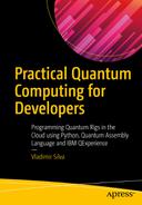
Under a virtual environment, Python packages will be installed in the environment’s home lib/python3.6/site-packages instead of the system’s path as shown in Figure 4-1.

../images/469026_1_En_4_Chapter/469026_1_En_4_Fig1_HTML.jpg — Figure 4-1
Python virtual environment folder layout

We are now ready to start writing quantum code. Let’s see how.

Qubit 101: It’s Just Basic Algebra

Before we start writing quantum programs, we need to refresh some fundamental mathematics to understand what goes on behind the scenes. In the previous chapter, you learned how a qubit is represented by the Bloch sphere: a geometrical representation of the pure state of a two-level quantum mechanical system (qubit). But perhaps a better way of understanding the basic model of the qubit and the effects of quantum gates is to use its algebraic representation. For this purpose you need to dust up some basic linear algebra concepts including

Linear vectors : Simple vectors such as $\left[\begin{array}{c}1\\ {}0\end{array}\right]$ which will be used to represent the basis states of the qubit.
Complex number : A complex number is a number composed of a real and imaginary parts denoted by a + bi where $i=\sqrt{-1}$ . Note that complex numbers cannot exist in our physical reality. The coefficients α, β of the super imposed state of a qubit ψ = α ∣ 0⟩+β ∣ 1⟩ are complex numbers.
Complex conjugate : A term that you will often hear when talking about quantum gates. To obtain a complex conjugate, simply flip the sign of the imaginary part; thus a + bi becomes a – bi and vice versa.
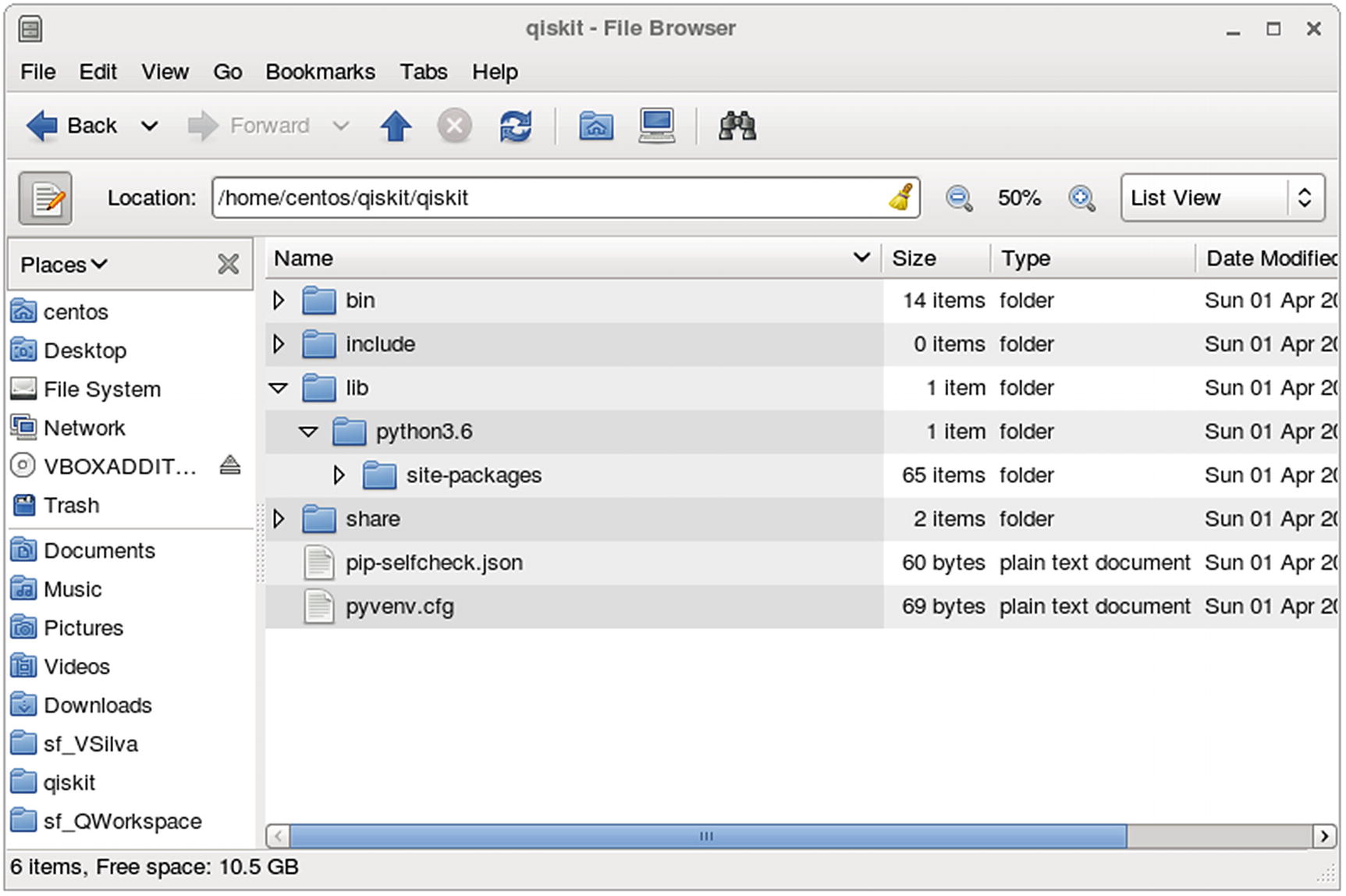
Matrix multiplication : If A is an n × m matrix and B is an m × p matrix, their product AB is an n × p matrix, in which the m entries across a row of A are multiplied with the m entries down a column of B and summed to produce an entry of AB. Take the first row from the first matrix and multiply each element for the first column of the second matrix, which becomes the first element in the result matrix (see Figure 4-2); but don’t panic, most of the matrices that we will be looking at are 2x2 consisting of 0 or 1 elements.

../images/469026_1_En_4_Chapter/469026_1_En_4_Fig2_HTML.jpg — Figure 4-2
Basic matrix multiplication operation

Algebraic Representation of a Quantum Bit

In the classical model, the fundamental unit of information is the bit which is represented by a 0 or 1. The bit physically translates to the voltage flow through a transistor. In quantum computation, the fundamental unit is the quantum bit (qubit) which physically translates to manipulations on photons, electrons, or atoms. Algebraically, the qubit is represented by the ket notation.

Tip

Ket notation was introduced in 1939 by physicist Paul Dirac and is also known as the Dirac notation. The ket is typically represented as a column vector and written as ∣φ⟩.

Dirac’s Ket Notation

Using Dirac’s notation, the basic quantum states of the qubit are represented by the vectors |0> and |1>. These are called the computational basis states.

Tip

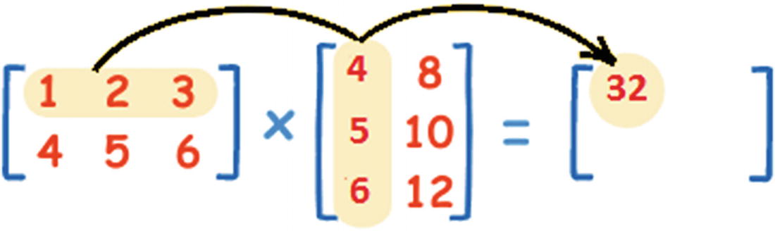
The quantum state of a qubit is a vector in a two-dimensional complex vector space. Let’s illustrate this with a simple graph.

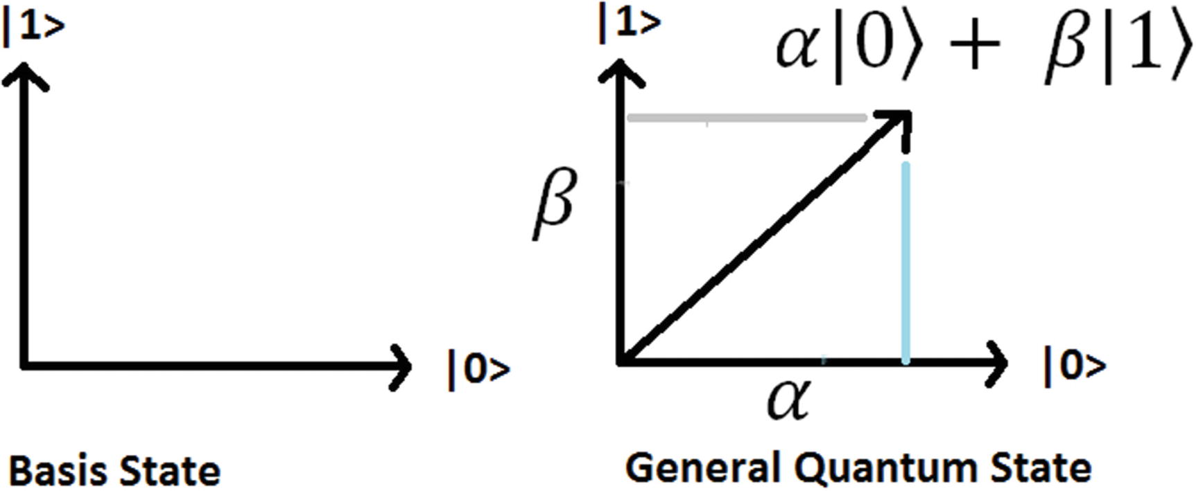
../images/469026_1_En_4_Chapter/469026_1_En_4_Fig3_HTML.jpg — Figure 4-3
Quantum states of the qubit

Figure 4-3 shows the complex vector space used to represent the state of a qubit. On the left side, the so-called basis state is made up of two unit vectors in the Dirac notation for the states |0> and |1>. On the right side, a general quantum state is made up of a linear combination of the two. Thus, the basis states and general quantum states can be written as vectors:

$\mid 0\left\rangle =\left[\begin{array}{c}1\\ {}0\end{array}\right],\mid 1\right\rangle =\left[\begin{array}{c}0\\ {}1\end{array}\right]$

$\alpha \mid 0\left\rangle +\beta \mid 1\right\rangle$

where α and β are amplitude coefficients of the unit vector. Note that a unit vector’s amplitude must be 1; therefore α and β must obey the constraint |α|² + |β|² = 1. This algebraic representation is the key to understanding the effect of a logic gate in the qubit as you will see later on.

So why is the state of a qubit represented as a vector in a seemly more complicated representation than its classical counterpart? Why vectors at all? The reason comes to that it allows for building a better model of computation as will be shown once we look at quantum gates and superposition of states. All in all, quantum mechanics is a theory that has evolved over many decades, and at the end of the day, a vector is a very simple mathematical object, easy to understand and manipulate. Probably the best tool for the job.

Superposition Is Just a Fancy Word

Superposition is defined by physicists as the property of atomic particles to exist in multiple states at the same time. If you find this concept difficult to grasp, then linear algebra can help.

Tip

Superposition is simply the linear combination of the |0> and |1> states. That is, α| 0⟩+β ∣ 1⟩ where the length of the state vector is 1 as shown in Figure 4-3.

Ket Notation Too Weird? Use Vectors Instead

If you like algebra and find the ket notation confusing, just use the familiar vector representation instead. Thus the superposition from the previous section can be written as

$\mid \varPsi \left\rangle =\alpha \mid 0\right\rangle +\beta \mid 1\Big\rangle =\alpha \left[\begin{array}{c}1\\ {}0\end{array}\right]+\beta \left[\begin{array}{c}0\\ {}1\end{array}\right]=\left[\begin{array}{c}\alpha \\ {}\beta \end{array}\right]$

Note that, because kets are vectors, they obey the same rules as vectors do, for example, multiplication by a scalar:

$2\left(\alpha |0\Big\rangle +\beta |1\Big\rangle \right)=2\left[\begin{array}{c}\alpha \\ {}\beta \end{array}\right]=\left[\begin{array}{c}2\alpha \\ {}2\beta \end{array}\right]$

Changing the State of a Qubit with Quantum Gates

The purpose of quantum gates is to manipulate the state of a qubit to achieve a desired result. They are the basic building blocks of quantum computation just as classic logic gates are for the classical world. Some the quantum gates are the equivalent of their classical counter parts. Let’s take a look.

NOT Gate (Pauli X)

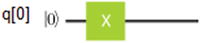
This is the simplest gate and it acts in a single qubit. It is the quantum equivalent of the classical NOT gate, and just like its counterpart, it flips the state of the qubit. Thus

|0⟩ → |1⟩, |1⟩ → |0⟩

For a superposition, the X gate acts linearly, meaning it flips the corresponding state; thus |0> becomes |1> and |1> becomes |0>:

$\alpha \mid 0\left\rangle +\beta \mid 1\right\rangle \to \alpha \mid 1\left\rangle +\beta \mid 0\right\rangle$

In a quantum circuit, the NOT gate is represented by the X also known as Pauli X, named after Austrian physicist Wolfgang Pauli, one of the fathers of quantum mechanics.

../images/469026_1_En_4_Chapter/469026_1_En_4_Figa_HTML.jpg

The circuit starts with the basis state |0> for qubit 0, the state flows through the quantum wire until a manipulation is done in the state, and then the output continues through the wire.

There is another way of looking at the X gate in action; by using its matrix representation, we can see exactly how the state is flipped by using the Pauli matrix

$X=\left[\begin{array}{cc}0& 1\\ {}1& 0\end{array}\right]$

The state of the qubit is flipped by using the matrix representation of X and the vectors for $\mid 0\Big\rangle =\left[\begin{array}{c}1\\ {}0\end{array}\right]$ and $\mid 1\Big\rangle =\left[\begin{array}{c}0\\ {}1\end{array}\right]$ ; thus

$X\kern0.28em \mid 0\left\rangle =\left[\begin{array}{cc}0& 1\\ {}1& 0\end{array}\right]\left[\begin{array}{c}1\\ {}0\end{array}\right]=\left[\begin{array}{c}0+0\\ {}1+0\end{array}\right]=\left[\begin{array}{c}0\\ {}1\end{array}\right]=\mid 1\right\rangle$

$X\kern0.28em \mid 1\left\rangle =\left[\begin{array}{cc}0& 1\\ {}1& 0\end{array}\right]\left[\begin{array}{c}0\\ {}1\end{array}\right]=\left[\begin{array}{c}0+1\\ {}0+0\end{array}\right]=\left[\begin{array}{c}1\\ {}0\end{array}\right]=\mid 0\right\rangle$

There is an even simpler quantum circuit, the simplest of them all, and it is the quantum wire denoted by the Greek symbol (Psi) ∣ψ⟩ _ _ _ _ _ _ _ _ _ ∣ ψ⟩ which describes the computational state over time. It may seem trivial, but physically this is the hardest thing to implement. Because of the atomic scale of the quantum wire (think photons, electrons, or single atoms), it is very fragile and prone to errors introduced by the environment.

Another interesting property of the X gate is that two NOT gates in a row give the identity matrix (I), a very important tool in linear transformations. Let’s do the math:

../images/469026_1_En_4_Chapter/469026_1_En_4_Figb_HTML.jpg

∣ψ⟩ → XX ∣ ψ⟩

To understand the effects of the circuit, let’s see what happens when we multiply two X matrices:

$XX=\left[\begin{array}{cc}0& 1\\ {}1& 0\end{array}\right]\left[\begin{array}{cc}0& 1\\ {}1& 0\end{array}\right]=\left[\begin{array}{cc}0+1& 0+0\\ {}0+0& 1+0\end{array}\right]=\left[\begin{array}{cc}1& 0\\ {}0& 1\end{array}\right]=I$

The X gate is the simplest example of a quantum logic gate, circuit, and computation. In the next section, we look at a truly quantum gate, Hadamard, and how it can trigger superpositions using circuits and algebra.

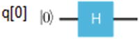
Truly Quantum: Superpositions with the Hadamard Gate

The effects of the Hadamard gate in the basis states are formally defined as

$\mid 0\left\rangle \to \frac{\left|0\Big\rangle +|1\right\rangle }{\sqrt{2}},\mid 1\right\rangle \to \frac{\left|0\Big\rangle -|1\right\rangle }{\sqrt{2}}$

Furthermore, for a superposition state α|0⟩+β|1⟩, the Hadamard maps to

$\alpha \mid 0\left\rangle +\beta \mid 1\right\rangle \to \alpha \left(\frac{\left|0\Big\rangle +|1\right\rangle }{\sqrt{2}}\right)+\beta \left(\frac{\left|0\Big\rangle -|1\right\rangle }{\sqrt{2}}\right)=\frac{\alpha +\beta }{\sqrt{2}}\mid 0\left\rangle +\frac{\alpha -\beta }{\sqrt{2}}\mid 1\right\rangle$

For the circuit and matrix presentation, the Hadamard acts on a single qubit.

../images/469026_1_En_4_Chapter/469026_1_En_4_Figc_HTML.jpg

$H=\frac{1}{\sqrt{2}}\left[\begin{array}{cc}1& 1\\ {}1& -1\end{array}\right]$

Applying H to the basis states $\mid 0\Big\rangle =\left[\begin{array}{c}1\\ {}0\end{array}\right]$ and $\mid 1\Big\rangle =\left[\begin{array}{c}0\\ {}1\end{array}\right]$ :

$H\mid 0\Big\rangle =\frac{1}{\sqrt{2}}\left[\begin{array}{cc}1& 1\\ {}1& -1\end{array}\right]\left[\begin{array}{c}1\\ {}0\end{array}\right]=\frac{1}{\sqrt{2}}\left[\begin{array}{c}1\\ {}1\end{array}\right]=\frac{1}{\sqrt{2}}\left(\left[\begin{array}{c}1\\ {}0\end{array}\right]+\left[\begin{array}{c}0\\ {}1\end{array}\right]\right)=\frac{\left|0\Big\rangle +|1\right\rangle }{\sqrt{2}}$

$H\mid 1\Big\rangle =\frac{1}{\sqrt{2}}\left[\begin{array}{cc}1& 1\\ {}1& -1\end{array}\right]\left[\begin{array}{c}0\\ {}1\end{array}\right]=\frac{1}{\sqrt{2}}\left[\begin{array}{c}1\\ {}-1\end{array}\right]=\frac{1}{\sqrt{2}}\left(\left[\begin{array}{c}1\\ {}0\end{array}\right]-\left[\begin{array}{c}0\\ {}1\end{array}\right]\right)=\frac{\left|0\Big\rangle -|1\right\rangle }{\sqrt{2}}$

So what is the computational reason for the Hadamard gate? What does this buy us? Without getting too technical, the answer is that the Hadamard gate expands the range of states that are possible for a quantum circuit. This is important because the expansion of states creates the possibility of finding shortcuts and therefore doing computations faster. An analogy would be to a game of chess. For example, if your knight was allowed to move like a queen and knight at the same time (an expansion of states), this will tilt the game in your favor and allow you to checkmate faster. This is what Hadamard gives: more horsepower to your quantum machine.

Measurement of a Quantum State Is Trickier Than You Think

Imagine you have a lab in the basement of your home. You are given a qubit in state |ψ⟩ = α|0⟩+β ∣ 1⟩ and a measurement apparatus and asked to calculate the α and β coefficients. That is, compute the quantum state. It may seem like a trivial task; however this is not possible. The principles of quantum mechanics state that the quantum state of a system is not directly observable. The best we can do is guess approximate information about α and β. This process is called measurement in the computational basis.

../images/469026_1_En_4_Chapter/469026_1_En_4_Figd_HTML.jpg

The outcome of a measurement on the quantum state |ψ⟩ = α|0⟩+β ∣ 1⟩ gives the classical bits:

α ∣ 0⟩+β ∣ 1⟩ → 0 with probality |∝²|

α ∣ 0⟩+β ∣ 1⟩ → 1 with probality |β²|

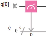
Thus the measurement process spits the probabilities of the classical bits 0 and 1 equal to the absolute values of the coefficients α and β squared. Physically, the way to imagine this process taking place is by observing a physical photon, atom, or electron with a measurement apparatus. This is the reason why measurement is often regarded as a quantum gate.

Measurement disturbs the state of the quantum system giving a classical bit outcome. The important thing to remember is that, after the process, the coefficients α and β are destroyed. This means that we cannot store large amounts of information in a qubit. Imagine if we could measure the exact values for α and β, then by using complex numbers it would be possible in theory to store infinite amounts of classical information in the qubit state. By calculating the exact values of α and β, we could extract all that classical information. However this is not possible. Quantum mechanics forbids it.

One final point on measurement is the normalization of the quantum state: given a measurement in the computational basis α ∣ 0⟩+β ∣ 1⟩, the probability of the classical bit 0 and 1 must add to 1. That is,

$Probality(0)+ Probality(1)=\mid {\propto}^2\mid +\mid {\beta}^2\mid =1$

This means that the length of the quantum state vector must be 1 (normalized). This comes from the fact that measurement probabilities add to 1. In the next section, we’ll talk about how single-qubit gates are generalized, what they are, and how they are used to build more complex circuits.

Generalized Single-Qubit Gates

So far we have seen two simple gates: X and H represented by the matrices:

$X=\left[\begin{array}{cc}0& 1\\ {}1& 0\end{array}\right],H=\frac{1}{\sqrt{2}}\left[\begin{array}{cc}1& 1\\ {}1& -1\end{array}\right]$

Remember also that the superposition of the quantum state is expressed as the vector $\mid \varPsi \Big\rangle =\left[\begin{array}{c}\alpha \\ {}\beta \end{array}\right]$ . Then applying both gates to the quantum state can be generalized for any unitary matrix:

$H\left[\begin{array}{c}\alpha \\ {}\beta \end{array}\right],\kern0.5em X\kern0.28em \left[\begin{array}{c}\alpha \\ {}\beta \end{array}\right],\kern0.5em U\left[\begin{array}{c}\alpha \\ {}\beta \end{array}\right]\kern0.28em where\kern0.28em U=H,X$

U is called the generalized single-qubit gate given the constraint that U must be unitary.

Tip

A matrix U is unitary if multiplied by its Hermitian transpose U ^† it gives the identity matrix: U ^† U = I. The Hermitian transpose or conjugate transpose is denoted by a dagger (†) symbol U ^† =(U^T )^∗, that is, the complex conjugate of the transposed.

The transpose of a matrix is a new matrix whose rows are the columns of the original. For example, if $A=\left[\begin{array}{cc}a& b\\ {}c& d\end{array}\right]\kern0.28em then\kern0.28em {A}^T=\left[\begin{array}{cc}a& c\\ {}b& d\end{array}\right]$ . Then, to obtain the Hermitian transpose A ^† $={\left[\begin{array}{cc}a& c\\ {}b& d\end{array}\right]}^{\ast }$ , take the complex conjugate of each entry. (The complex conjugate of a + bi, where a and b are real, is a – bi, that is, switch the sign of the imaginary part if any.)

Note that both gates H and X must be unitary. This can be easily verified by calculating X ^† X = I and H ^† H = I:

$X=\left[\begin{array}{cc}0& 1\\ {}1& 0\end{array}\right]$ X ^† = $\left[\begin{array}{cc}0& 1\\ {}1& 0\end{array}\right]\to$ X ^† X = XX = I

$H=\frac{1}{\sqrt{2}}\left[\begin{array}{cc}1& 1\\ {}1& -1\end{array}\right]$ H ^† = $\frac{1}{\sqrt{2}}\left[\begin{array}{cc}1& 1\\ {}1& -1\end{array}\right]\to$ H ^† H = HH = I

Unitary Matrices Are Good for Quantum Gates

A question that arises from the previous section: Why go through all the trouble? Why do X and H need to be unitary? The answer is that unitary matrices preserve vector length. This is useful for quantum gates because these require input and output states to be normalized (have a vector length of 1). In fact unitary matrices are the only type of matrices that preserve length and therefore the only type of matrix that can be used for quantum gates. All in all, a deeper question arises: why should quantum gates be linear in the first place and why use a matrix representation at all? We’ll try to answer this in a later section, but for now, we’ll just have to accept it.

Other Single-Qubit Gates

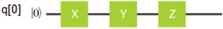
In the previous section, we saw the single-qubit gates X and H. At the same time, there are other single-qubit gates that are useful in quantum computation.

The X gate has two partners Y, Z. These form the trio known as the Pauli Sigma (σ) gates.

../images/469026_1_En_4_Chapter/469026_1_En_4_Fige_HTML.jpg

$X=\left[\begin{array}{cc}0& 1\\ {}0& 1\end{array}\right],Y=\left[\begin{array}{cc}0& -i\\ {}i& 1\end{array}\right],Z=\left[\begin{array}{cc}1& 0\\ {}0& -1\end{array}\right]$

These three matrices are useful for information processing tasks such as super dense coding (SDC), a process that seeks to store classical information efficiently in a qubit. They also come up when analyzing atomic properties such as electron spin. Plus they are closely related to the three dimensions of space XYZ.

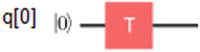
The rotation gate

../images/469026_1_En_4_Chapter/469026_1_En_4_Figf_HTML.jpg

$\left[\begin{array}{cc}\cos \kern0.28em \theta & -\sin \theta \\ {}\sin \theta & \cos \theta \end{array}\right]$

It is the familiar rotation on real space by an angle θ. This is a unitary matrix, and in this particular case, the T gate performs a Π/4 rotation around the Z-axis. This gate is required for universal control.

Gates can also manipulate many qubits as we’ll see in the next section.

Qubit Entanglement with the Controlled NOT Gate

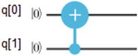
This gate completes the arsenal of quantum gates required for quantum computation. The controlled NOT (CNOT) is a 2-qubit gate with four computational basis states.

For a superposition, the four basis states CNOT gives

α ∣ 00⟩+β ∣ 01⟩+δ ∣ 10⟩+γ ∣ 11⟩

where α (alpha), β (beta), δ (delta), and γ (gamma) are the superposition coefficients. The quantum circuit is shown as follows:

../images/469026_1_En_4_Chapter/469026_1_En_4_Figg_HTML.jpg

The matrix representation of CNOT for the basis states is given by

$\left[\begin{array}{cccc}1& 0& 0& 0\\ {}0& 1& 0& 0\\ {}0& 0& 0& 1\\ {}0& 0& 1& 0\end{array}\right]$

∣00⟩

∣01⟩

∣10⟩

∣11⟩

The plus (+) symbol is called the target qubit, and the blue dot (below it) is the control qubit. What it does is simple:

• If the control qubit is set to 1, then it flips the target qubit.

• Otherwise it does nothing.

To be more precise, if the first bit is the control, then

∣00⟩ → ∣ 00⟩ contol 0 do nothing

∣01⟩ → ∣ 01⟩ contol 0 do nothing

∣10⟩ → ∣ 11⟩ control 1 flip 2nd

∣11⟩ → ∣ 10⟩ control 1 flip 2nd

An easy representation of the preceding states is ∣xy⟩ → ∣ x y ⊕ x⟩

Tip

The CNOT gate is required to generate entanglement, and it is critical in all kinds of tasks including quantum teleportation, super dense coding, and almost any quantum algorithm out there.

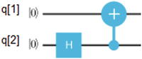
For example, to entangle 2 qubits, apply the Hadamard gate (H) to the first qubit and then apply the CNOT to the second qubit as shown in the following:

../images/469026_1_En_4_Chapter/469026_1_En_4_Figh_HTML.jpg

For the basis state in qubit (2), the Hadamard gives

$\mid 00\Big\rangle \to \frac{\left|00\Big\rangle +|10\right\rangle }{\sqrt{2}}$

After applying the CNOT, we flip the second qubit if the control is 1, thus

$\mid 00\Big\rangle \to \frac{\left|00\Big\rangle +|11\right\rangle }{\sqrt{2}}$

This effectively creates an entangled state between qubits 1 and 2.

All in all, CNOT and single-qubit gates are a powerful arsenal for quantum computation. Because they build up unitary operations on any number of qubits, they are said to be universal for quantum computation. This means that to build a quantum computer that can solve any quantum task, it is enough to use single-qubit gates along with CNOT and measurement gates.

Universal Quantum Computation Delivers Shortcuts over Classical Computation

You may wonder how all the circuits and algebra in the preceding section can help in solving computation tasks that can be easily performed, and probably cheaper, in a classical system. If you consider the so-called bit strength of a classical system

$x\to f(x)$

where, given some input x, the goal is to compute a function f(x) with at least 2^k-1 elementary operations (where k is the bit strength), then the universal quantum computation can provide an equivalent circuit of roughly the same size that contains the same classical model:

$\mid x\left\rangle, 0\to \mid x\right\rangle, f(x)$

What is exciting about the preceding circuit is that there are sometimes shortcuts provided by the greater power of quantum computation to get results faster. This means that you can compute f(x) in fewer than 2^k-1 operations. For some quantum algorithms such as factorization, the speedups are exponential! This is the true power of quantum systems. So now that you have explored the basic mathematical model of a quantum circuit, it is time to switch into programmatic mode and see how all this can be turned into an actual computer program to be executed on a real quantum device.

Your First Quantum Program

Let’s look at the anatomy of a quantum program with a bare-bones example. In this example, we create a single qubit, one classic register to measure the qubit, and then we apply the Pauli X gate (bit flip) on the qubit and finally measure its value. The basic pseudocode of the program can be resumed as follows:

1.
Create a quantum program.
2.
Create one or more qubits and classical registers to measure the qubits.
3.
Create a circuit which groups the qubits in a logical execution unit.
4.
Apply quantum gates on the qubits to achieve a desired result.
5.
Measure the qubits into the classical register to collect a final result.
6.
Compile the program. This step creates a JSON representation of the program in a specific format that will be described later on in this section.
7.
Run in the simulator or real quantum device.
8.
Fetch the results.

Now let’s look at the Python code as well as the Composer circuit in detail.

#############################

import sys

import qiskit

import logging

from qiskit import QuantumProgram

# Main sub

def main():

# create a program

qp = QuantumProgram()

# create 1 qubit

quantum_r = qp.create_quantum_register("qr", 1)

# create 1 classical register

classical_r = qp.create_classical_register("cr", 1)

# create a circuit

qp.create_circuit("Circuit", [quantum_r], [classical_r])

# get the circuit by name

circuit = qp.get_circuit('Circuit')

# enable logging

qp.enable_logs(logging.DEBUG);

# Pauli X gate to qubit 1 in the Quantum Register "qr"

circuit.x(quantum_r[0])

# measure gate from qubit 0 to classical bit 0

circuit.measure(quantum_r[0], classical_r[0])

# backend simulator

backend = 'local_qasm_simulator'

# Group of circuits to execute

circuits = ['Circuit']

# Compile your program

qobj = qp.compile(circuits, backend)

# run in simulator

result = qp.run(qobj, timeout=240)

# Show result counts

print (str(result.get_counts('Circuit')))

###########################################

# Linux :main()

# windows

if __name__ == '__main__':

main()

Listing 4-3

Anatomy of a Quantum Program

Let’s see what is going on in Listing 4-3:

Lines 2–5 import the required libraries: sys (system), qiskit (quantum classes), logging (for debugging), and QuantumProgram: the foundation class for all programs.
Next, line 11 creates a QuantumProgram. This is the access point to all operations.
To create a qubit list, use the quantum program create_quantum_register(NAME, SIZE) system call where NAME is the name of the register list and SIZE is the number of qubits. In this case 1 (line 14).
For each qubit, create a classical register to perform a measurement using the system call create_classical_register(NAME, SIZE).
Next, create a circuit with the system call create_circuit(NAME, QUANTUM_SET,CLASSIC_SET) where NAME is the name of the circuit, QUANTUM_SET is a list of qubits, and CLASSIC_SET is the list of classic registers. A circuit is the logical unit that holds all qubits and classical registers (line 20).
Optionally, enable debugging with the system call enable_logs(LEVEL) where LEVEL can be one of logging.DEBUG, logging.INFO, etc. (just the usual logging stuff).
Next, run the qubit(s) through quantum gates and perform measurements on the qubit(s) to collect results. In this case we apply the Pauli X gate which flips the qubit from its ground state |0> to |1> (lines 25–29).
Finally, compile the program and run the simulator or real device. In this case we run in the local Python simulator (local_qasm_simulator) (lines 37–41).

Windows developers watch out! You must wrap your program in a main function and then call it with

if __name__ == '__main__':

main()

This is required in Windows because QISKit executes the program using asynchronous tasks (executors), and when the task fires, the subprocess will execute the main module at startup. Thus you need to protect the main code to avoid creating subprocesses recursively. I found this out the hard way when my programs run properly in CentOS but failed in Windows with

RuntimeError:

An attempt has been made to start a new process before the

current process has finished its bootstrapping phase.

This probably means that you are not using fork to start your

child processes and you have forgotten to use the proper idiom

in the main module:

if __name__ == '__main__':

freeze_support()

...

The "freeze_support()" line can be omitted if the program

is not going to be frozen to produce an executable.

This can be a source of grief for the newcomer to Python. Now, run the program to see the output:

INFO:qiskit._jobprocessor:<qiskit._result.Result object at 0x000000000D99F470>

{'1': 1024}

The result is the JSON document {'1': 1024} where 1 is the measurement of the qubit (remember that we used an X gate to flip the bit) and 1024 is the number of iterations of that result. The probability of this result is calculated by dividing the number of the result iterations (1024) by the total number of iterations of the program (1024). In this case P = 1024/1024 = 1.

Tip

Quantum computers are probabilistic machines. Thus all measurements come attached with a probability for that specific result.

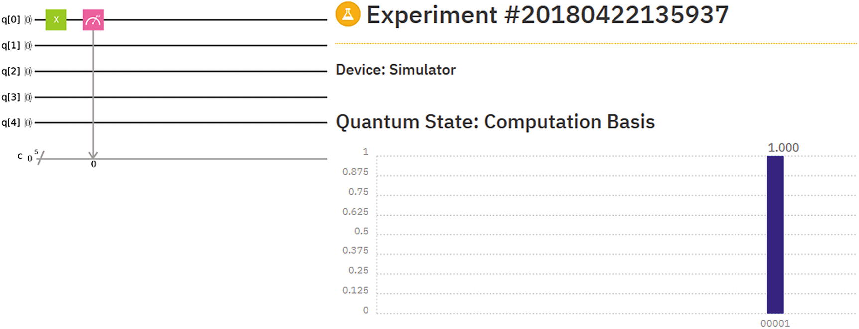
Listing 4-3 can also be described with an equivalent quantum circuit quickly constructed and executed in the IBM Q Experience Composer as shown in Figure 4-4.

../images/469026_1_En_4_Chapter/469026_1_En_4_Fig4_HTML.jpg — Figure 4-4
Composer experiment for Listing 4-3

Figure 4-4 shows the quantum circuit for Listing 4-3 including the result of the experiment as well as the attached probability. The circuit is very simple as you can see: in the Composer, drag an X gate over qubit 0, then perform a measurement on the same qubit. You will find the Composer a wonderful tool to construct relatively simple circuits, execute them, and visualize their results! Now let’s peek into the SDK internals to see how this code gets massaged behind the scenes.

SDK Internals: Circuit Compilation and QASM

Figure 4-5 shows what goes on behind the scenes when your program is run:

QISKit compiles your program’s circuit(s) into a JSON document to be submitted to the local simulator.
The simulator parses the document, runs the circuit, and returns an opaque JSON document (hidden from the developer).
QISKit wraps the results JSON document in an object available to the main program. For example, a call to result.get_counts('Circuit') extracts the count information from this document.

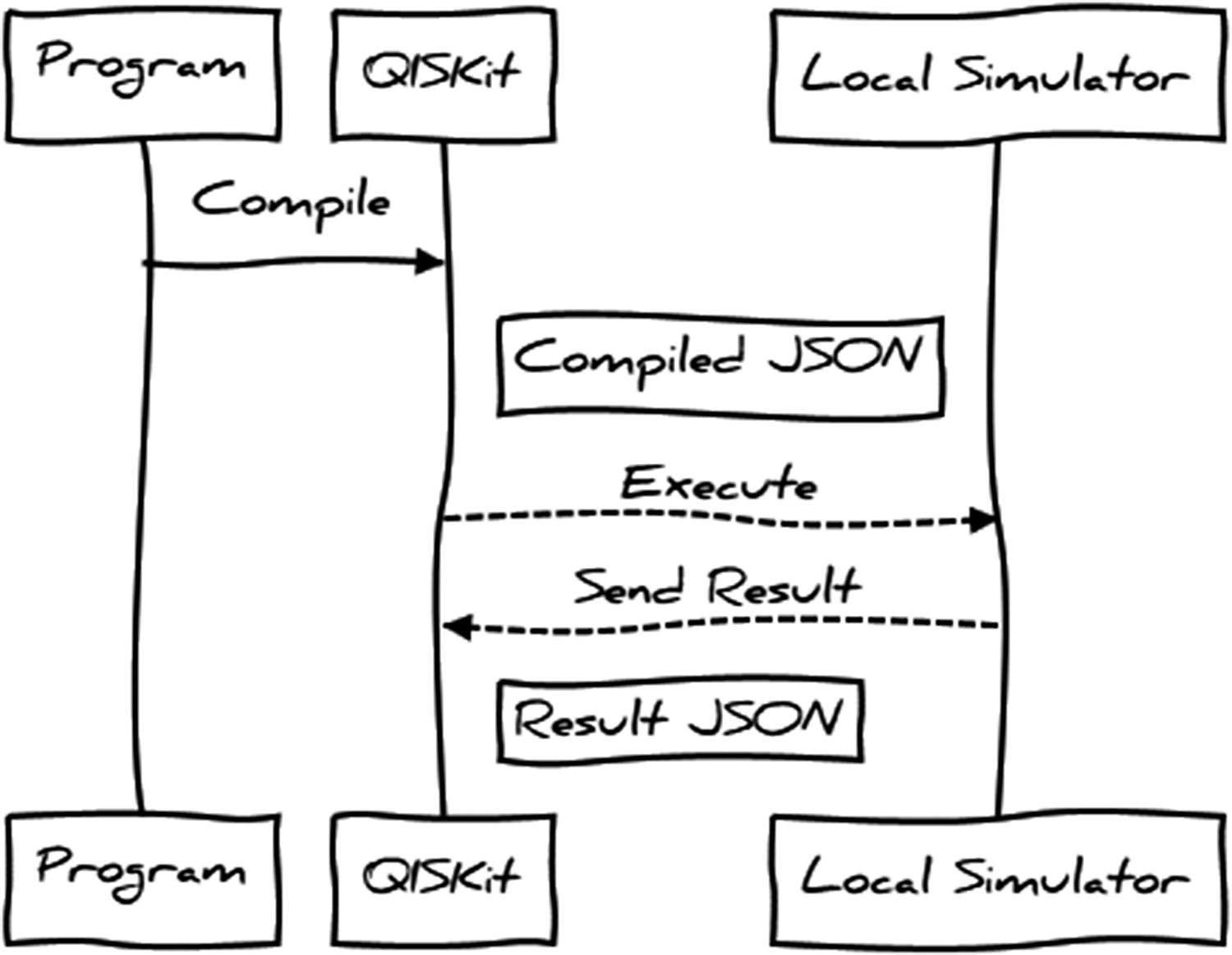
../images/469026_1_En_4_Chapter/469026_1_En_4_Fig5_HTML.jpg — Figure 4-5
Sequence diagram between the program, QISKit, and local simulator

Circuit Compilation

Listing 4-4 shows the format of the compiled program before submission to the simulator. The document is made up of

An execution id
A header with information about the simulator including name, number of credits used in the execution, plus number of run interactions (shots)
The circuit section contains an array of circuit objects. Each circuit is made of
- A circuit name
- A header (config) with information such as qubit coupling map, basis (physical) gates, runtime seed, and more
- A compiled circuit section with a header containing information about the qubits and classical registers, as well as an array of operation (or gates) applied to the circuit and their parameters

{

"id": "aA46vJHgnKQko3u5L1QqbUDk31sY2m",

"config": {

"max_credits": 10,

"backend": "local_qasm_simulator",

"shots": 1024

"circuits": [{

"name": "Circuit",

"config": {

"coupling_map": "None",

"layout": "None",

"basis_gates": "u1,u2,u3,cx,id",

"seed": "None"

"compiled_circuit": {

"operations": [{

"name": "u3",

"params": [3.141592653589793, 0.0, 3.141592653589793],

"texparams": ["\\pi", "0", "\\pi"],

"qubits": [0]

}, {

"name": "measure",

"qubits": [0],

"clbits": [0]

}],

"header": {

"number_of_qubits": 1,

"qubit_labels": [

["qr", 0]

"number_of_clbits": 1,

"clbit_labels": [

["cr", 1]

]

}

"compiled_circuit_qasm": "OPENQASM 2.0;\ninclude \"qelib1.inc \";\nqreg qr[1];\ncreg cr[1];\nu3(3.14159265358979,0,3.14159265358979) qr[0];\nmeasure qr[0] -> cr[0];\n"

}]

}

Listing 4-4

Compilation Format for Listing 4-3

To display the compiled circuit within your program, print the result of the compilation step as shown in the following command:

qobj = qp.compile(circuits, backend)

print(str(qobj))

Note

The compilation format is opaque to the programmer and not meant to be accessed directly, but via the SDK API. The reason is that its format may change from version to version. However it is always good to understand what occurs behind the scenes.

Execution Results

This is the response document from the local simulator to the QISKit. The format of this document is shown in Listing 4-5. Remarkable information includes

Status of the run, execution time, simulator name, and more.
Result data. This is the information available within your program with the call: print (str(result.get_counts('Circuit'))).

{

"backend": "local_qiskit_simulator",

"id": "aA46vJHgnKQko3u5L1QqbUDk31sY2m",

"result": [{

"data": {

"counts": {

"1": 1024

"time_taken": 0.0780002

"name": "Circuit",

"seed": 123,

"shots": 1024,

"status": "DONE",

"success": true,

"threads_shot": 4

}],

"simulator": "qubit",

"status": "COMPLETED",

"success": true,

"time_taken": 0.0780002

}

Listing 4-5

Results Document from Local Simulator

Obtaining the results document is a bit trickier because it is an opaque object not exposed to the user’s program. Nevertheless you could save the compiled circuit from the previous section and feed it to the simulator manually to obtain the result shown in Listing 4-5. This task is left to you however. The important thing to remember is that the results document (as well as the compilation format) is opaque to the programmer. The reason is that their formats may change over time; nonetheless it is always helpful to understand how things work behind the scenes.

Tip

The compilation and results formats are useful for simulator developers. For example, you could save compilation and results formats for a sample circuit, fix a bug in the C++ simulator, feed it, and compare its results. In this way, your simulator could be easily integrated with the SDK for the rest of us to play with.

Assembly Code

The compiled circuit in Listing 4-4 includes a section that contains a translation of the program into quantum assembly (QASM) as shown in the next paragraph.

OPENQASM 2.0;

include "qelib1.inc";

qreg qr[1];

creg cr[1];

x qr[0];

measure qr[0] -> cr[0];

Tip

QASM is useful only if running in the remote simulator provided by IBM Q Experience.

QISKit Local Simulators

Access to real quantum devices in IBM Q Experience is restricted by a credit system that diminishes with use; thus we shouldn’t run trivial programs such as Listing 4-3. For this purpose QISKit packs a plethora of simulators to satisfy all your testing needs. Table 4-1 provides a list of local and remote simulators available via QISKit and IBM Q Experience by the time of this writing.

Table 4-1

List of Local and Remote Simulators for IBM Q Experience

Name	Description
local_qasm_simulator	This is the default Python simulator bundled with QISKit. It is very slow but does the job.
local_clifford_simulator also known as local_qiskit_simulator	A high-performance simulator written in C++ with realistic noise and error simulation.
ibmqx_qasm_simulator	A 24-qubit high-performance remote QASM simulator provided by Q Experience. This is the default remote simulator.
ibmqx_hpc_qasm_simulator	A 32-qubit mega powerful parallel simulator provided by Q Experience. This is a backup to the default remote simulator.

As a simple exercise, obtain a list of IBM Q Experience simulators and real devices by pasting the following REST API URL into your browser:

https://quantumexperience.ng.bluemix.net/api/Backends?access_token=ACCESS_TOKEN.

Of course you need an access token which can be easily obtained using the Remote Access API from Chapter 3. Next, let’s run our program in other local simulators including the IBM Q Experience remote simulator. Finally let’s time our runs to see which simulator is the fastest.

Running in the Local C++ simulator

QISKit uses the pure Python simulator as default (local_qasm_simulator). However you can also use a fast C++ simulator with realistic noise and error rates by changing the backend name of your program to local_clifford_simulator or local_qiskit_simulator (line 35 in Listing 4-3). However there are some caveats you should keep in mind before using it:

Linux users: This simulator uses the C++11 standard which requires gcc 5.3 or later. As a matter of fact the simulator was not built in my CentOS 6 and 7 systems. (you may want to use Windows in this instance).
Windows users: Python uses the CMake utility to build the simulator on the fly. All in all, the default source does not provide a Visual Studio solution to build in Windows. Nevertheless I have taken the time to provide one and fix a couple of crashes I encountered in Windows 7.

Tip

A Windows 64-bit binary for the C++ simulator can be found in the book source under Ch04\qiskit-simulator\qiskit-simulator\x64\Debug. A Visual Studio 2017 solution is also provided if you wish to build it yourself. Make sure you copy all the files in this folder to PYTHON-HOME\Lib\site-packages\qiskit\backends if missing.

Running in a Remote Simulator

To run in the remote simulator provided by IBM Q Experience, Listing 4-3 needs to change a little bit. Let’s see how:

The first thing we need is an IBM Q Experience configuration descriptor with the execution parameters as shown in the next paragraph:

APItoken = 'YOU-API-TOKEN'

config = {

'url': 'https://quantumexperience.ng.bluemix.net/api',

# The following should only be needed for IBM Q users.

'hub': 'MY_HUB',

'group': 'MY_GROUP',

'project': 'MY_PROJECT'

}

Tip

The preceding code should be kept in a separate file (Qconfig.py) in the same folder as the main program. Get your API token from the IBM Q Experience web console (as shown in Chapter 3) and paste it in the code. Note that hub, group, and project are required for corporate customers only.

Next import the preceding descriptor into the main program:

# Q Experience config

import Qconfig

# Main sub

def main():

Finally switch the execution backend to the remote simulator:

1.
Change the backend name to ibmq_qasm_simulator.
2.
Tell the quantum program to use IBM Q Experience by setting the API parameters with the system call: qp.set_api(Qconfig.APItoken, Qconfig.config['url']) where APItoken and URL are the values from the configuration descriptor.
3.
Execute in IBM Q Experience with the system call: result = qp.execute(circuits, backend, shots=512, max_credits=3). Note that we do not compile and run the circuit as before. Therefore you must remove the calls to qobj = qp.compile(circuits, backend) and result = qp.run(qobj, wait=2, timeout=240).

The changes are shown in the following command. Make sure you remove the old compilation and run calls or the program will fail:

backend = 'ibmqx_qasm_simulator'

# Group of circuits to execute

circuits = ['Circuit']

# set the APIToken and Q Experience API url

qp.set_api(Qconfig.APItoken, Qconfig.config['url'])

result = qp.execute(circuits, backend, shots=512, max_credits=3, wait=10, timeout=240)

Finally, execute and test. The output should look something like

DEBUG:qiskit.backends._qeremote:Running on remote backend ibmq_qasm_simulator with job id: 3677ff592e5e5a6fd31a569b0b4faf92

INFO:qiskit._jobprocessor:<qiskit._result.Result object at 0x0000000004A35160>

{'1': 512}

Now let’s put all this together and see who the fastest simulator is. My money is in C++.

And the Fastest Simulator Is Comparing Execution Times

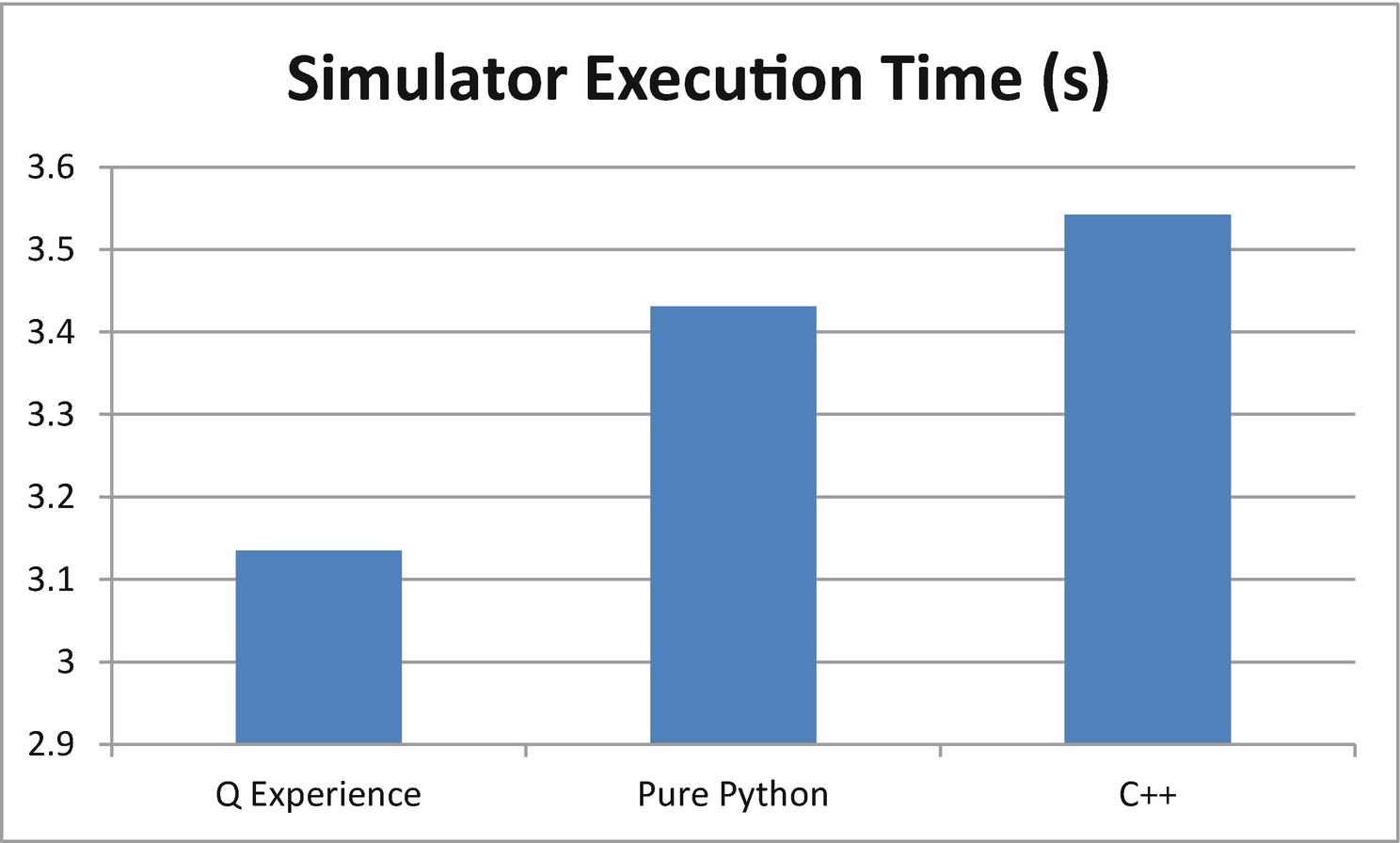
I have gathered execution times for all simulators in an x64 machine running Windows 7. Incredibly, the fastest simulator turned out to be the IBM Q Experience remote, followed closely by the pure Python, and lastly my personal favorite: C++ (see Figure 4-6).

../images/469026_1_En_4_Chapter/469026_1_En_4_Fig6_HTML.png — Figure 4-6
Execution times for QISKit simulators

Even though the call goes through the network, the IBM Q Experience remote simulator manages to outperform the others. What I found perplexing is how an interpreted Python simulator can be faster than a native code implementation. This is probably due to the fact that the native invocation uses asynchronous tasks to spawn the C++ simulator process, thus slowing things down enough for the Python code to outperform it. Now that you have learned how to run a program in the simulator, let’s do it in the real thing.

Running in a Real Quantum Device

Let’s modify the program from the previous section to make a more complex circuit instead. Listing 4-6 shows a sample circuit that performs a series of rotations on the first qubit of a quantum computer. The rotations demonstrate the use of the physical gates of the real quantum processor ibmqx4: u1, u2, and u3 to rotate a single qubit over the X-, Y-, and Z-axis of the Bloch sphere by theta, phi, or lambda degrees.

Tip

The Bloch sphere is the geometrical representation of a single qubit where the top of the Z-axis represents the basis state |0> and the bottom |1>. A rotation over a given axis represents the probability that the qubit will collapse in certain direction when a measurement is performed (see Figure 4-7).

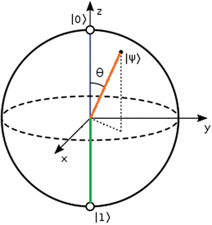
../images/469026_1_En_4_Chapter/469026_1_En_4_Fig7_HTML.jpg — Figure 4-7
Bloch sphere representation of a qubit

Physical gates (also known as basis gates) are important because they constitute the foundation under which more complex logical gates are constructed. Hence Listing 4-6 performs the following steps:

It allocates 5 qubits and five classical measurement registers corresponding to the 5 qubits available from the ibmqx4 processor in Q Experience (lines 17–20).
Next, a sequence of rotations on the first qubit are performed using the basis gates u1, u2, and u3 (lines 29–34).
Finally, a measurement is performed in the qubit and the result stored in the classical register.
Before execution the backend is set to ibmqx4 (a 5-qubit processor – line 42), and the authentication token and API URL are set via set_api(Qconfig.APItoken, Qconfig.config['url']).
To execute in the real quantum device, use the QuantumProgram execute system call execute(NAMES, BACKEND, shots=SHOTS, max_credits=CREDITS, timeout=TIMEOUT) where
- NAMES is a list of circuit names.
- SHOTS is the number of iterations performed in the circuit. The higher the number, the greater the accuracy.
- CREDITS is the maximum number of points that you wish to be deducted from your execution bank (15 is the default startup number). Note that the more shots are performed, the more credits will be deducted from your bank. Keep this in mind before you run out of credits.
- TIMEOUT is the read timeout from the remote end point.

Note

Python quantum programs/experiments executed against a real device are not recorded in the Composer-Scores section of IBM Q Experience. This is because Python uses the Jobs REST API behind the scenes which puts the experiment in an execution queue instead. If you wish to record your executions in the Composer, you could use the web console or REST APIs as shown in the next section.

import sys,time,math

import qiskit

import logging

from qiskit import QuantumProgram

# Q Experience config

import Qconfig

# Main sub

def main():

# create a program

qp = QuantumProgram()

# create 1 qubit

quantum_r = qp.create_quantum_register("qr", 5)

# create 1 classical register

classical_r = qp.create_classical_register("cr", 5)

# create a circuit

circuit = qp.create_circuit("Circuit", [quantum_r], [classical_r])

# enable logging

qp.enable_logs(logging.DEBUG);

# first physical gate: u1(lambda) to qubit 0

circuit.u2(-4 *math.pi/3, 2 * math.pi, quantum_r[0])

circuit.u2(-3 *math.pi/2, 2 * math.pi, quantum_r[0])

circuit.u3(-math.pi, 0, -math.pi, quantum_r[0])

circuit.u3(-math.pi, 0, -math.pi/2, quantum_r[0])

circuit.u2(math.pi, -math.pi/2, quantum_r[0])

circuit.u3(-math.pi, 0, -math.pi/2, quantum_r[0])

# measure gate from qubit 0 to classical bit 0

circuit.measure(quantum_r[0], classical_r[0])

circuit.measure(quantum_r[1], classical_r[1])

circuit.measure(quantum_r[2], classical_r[2])

# backend

backend = 'ibmqx4'

# Group of circuits to execute

circuits = ['Circuit']

# set the APIToken and Q Experience API url

qp.set_api(Qconfig.APItoken, Qconfig.config['url'])

result = qp.execute(circuits, backend, shots=512, max_credits=3, timeout=240)

# Show result counts

print ("Job id=" + str(result.get_job_id()) + " Status:" + result.get_status())

###########################################

if __name__ == '__main__':

start_time = time.time()

main()

print("--- %s seconds ---" % (time.time() - start_time))

Listing 4-6

Sample Circuit #2

Quantum Circuit for the Composer

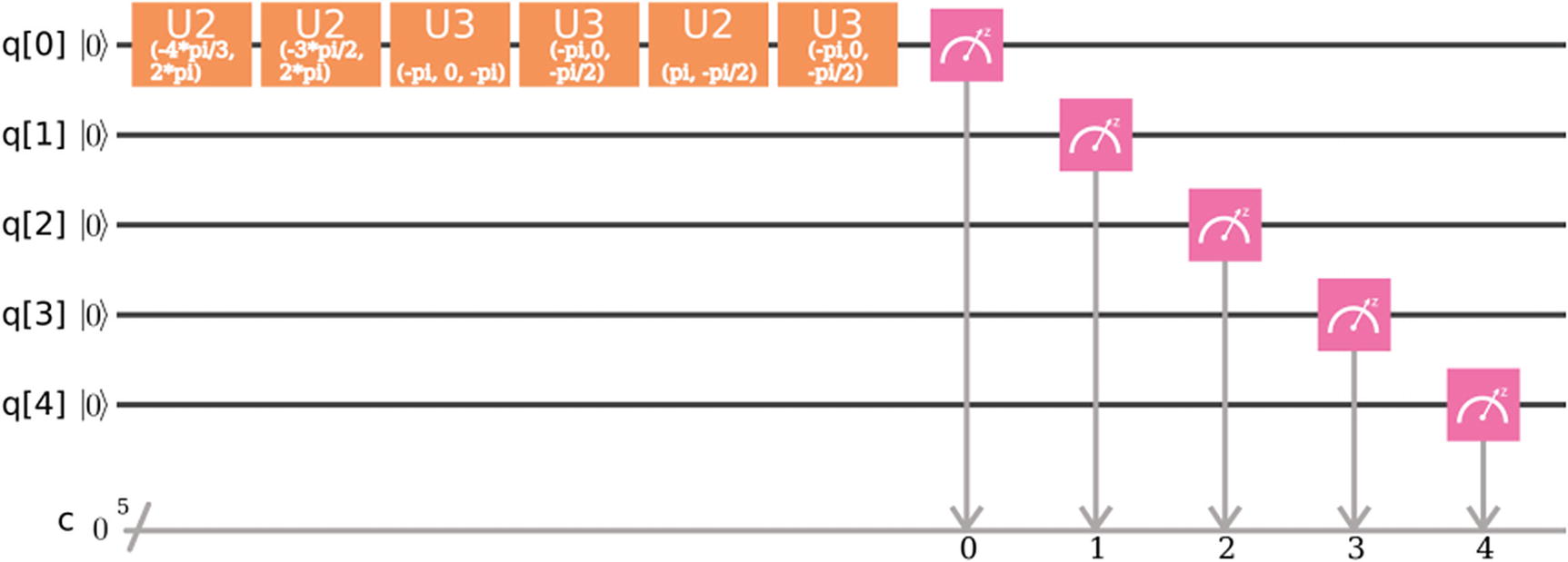
The program in Listing 4-6 can also be created in the IBM Q Experience Composer using their slick drag and drop user interface. Simply drag the gates into the qubit histogram as shown in Figure 4-8, set the parameters for the gate(s), and finally save and run in the simulator or real device.

../images/469026_1_En_4_Chapter/469026_1_En_4_Fig8_HTML.jpg — Figure 4-8
Q Experience Composer circuit for Listing 4-6

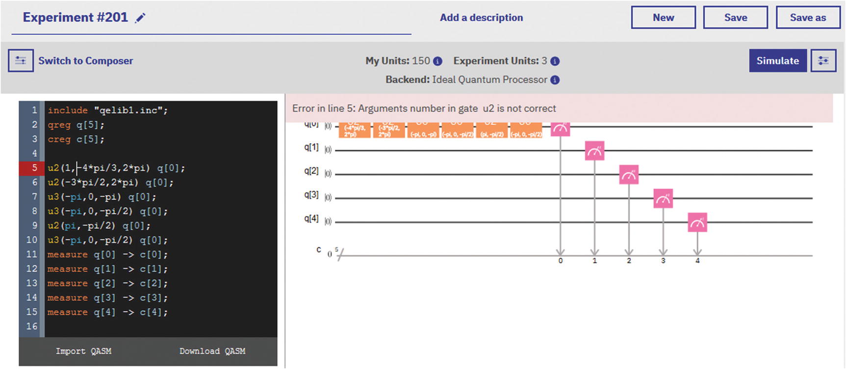
For those of you who prefer the raw power of assembly, the Composer allows to copy-paste code directly into the console in assembly mode as shown in Figure 4-9. It will even parse any syntax errors in your code and show you the offending line(s).

../images/469026_1_En_4_Chapter/469026_1_En_4_Fig9_HTML.jpg — Figure 4-9
Composer in assembly mode for circuit in Figure 4-8

There are multiple ways of executing your experiment in IBM Q Experience; one of the most interesting is using their awesome REST API.

Execution via Your Favorite REST Client

This is one of the most exciting ways to interact with Q Experience. By using simple REST requests, you can do pretty much anything you do in Python or the Composer:

List backend devices.
List hardware or calibration parameters for the real devices.
Get information about the job execution queue.
Get the status of a job or experiment.
Push or cancel jobs.
Execute an experiment and record it in the Scores section of the Composer.

Tip

The REST API allows you to use any language to create your own interface to Q Experience (even a web browser). This API is described in full detail in Chapter 3.

There are two ways of submitting experiments using REST: via the jobs and the execute APIs. Let’s see how.

Run via the Jobs API

You can use your favorite browser REST client to submit the experiment in Listing 4-6. For example, using Chrome’s YARC (Yet Another REST Client) create an HTTP POST request to the end point:

https://quantumexperience.ng.bluemix.net/api/Jobs?access_token=ACCESS_TOKEN

The tricky part is getting your access token or access key. For this part you must authenticate using your API token or username and password. Note that the API token is not to be confused with the access token. To obtain an access token, you must do an authentication request. (Take a look at Chapter 3 under “Remote Access via the REST API.”)

Tip

Chrome’s YARC allows you to construct REST requests and save them as favorites. Create an authentication request to IBM Q Experience as described in Chapter 3, save it as a favorite, and use it every time to obtain an access token to test other REST API calls.

The request payload is a JSON document shown in Listing 4-7. The format is described in Table 4-2.

Table 4-2

Request Format for the Jobs API

Key	Description
qasms	This is an array of assembly code programs all in one line separated by the line feed character (\n).
Shots	The number of iterations you code will go through.
backend	This is an object that describes the backend. In this case ibmqx4.
maxCredits	This is a hint of the number of credits to be deducted from your account balance.

{

"qasms": [{

"qasm": "\n\ninclude \"qelib1.inc\";\nqreg q[5];\ncreg c[5];\nu2(-4*pi/3,2*pi) q[0];\nu2(-3*pi/2,2*pi) q[0];\nu3(-pi,0,-pi) q[0];\nu3(-pi,0,-pi/2) q[0];\nu2(pi,-pi/2) q[0];\nu3(-pi,0,-pi/2) q[0];\nmeasure q -> c;\n"

}],

"shots": 1024,

"backend": {

"name": "ibmqx4"

"maxCredits": 3

}

Listing 4-7

HTTP Request for the Jobs API

Once you have obtained an access token, copy-paste the payload from Listing 4-7 into your REST client, submit, and wait for a response. If all goes well, you should see a response similar to Listing 4-8.

{

"qasms": [

{

"status": "WORKING_IN_PROGRESS",

"executionId": "e9d758c3480a54a6455f72c84c5cc2a6"

}

"shots": 1024,

"backend": {

"id": "c16c5ddebbf8922a7e2a0f5a89cac478",

"name": "ibmqx4"

"status": "RUNNING",

"maxCredits": 3,

"usedCredits": 3,

"creationDate": "2018-04-24T00:12:07.847Z",

"deleted": false,

"id": "33d58594fcb7204e4d2ccdb65cd3c88c",

"userId": "ef072577bd26831c59ddb212467821db"

}

Listing 4-8

HTTP Response from Q Experience

A partial response format is described in Table 4-3.

Table 4-3

Response Format for the Jobs API

Key	Description
qasms	An array of objects that includes The submitted code. The runtime status: WORKING_IN_PROGRESS, COMPLETED, or FAILED. An execution id for the code.
shots	The number of iterations of the experiment.
backend	An object with information about the backend such as name and id.
status	The overall status of the job: RUNNING, COMPLETED, or FAILED.
maxCredits	The maximum number of credits used for this run.
usedCredits	The actual number of credits spent in this run.
creationDate	Date the job was created.
deleted	True if a request to delete the job has been submitted, else false. Note: Canceled or deleted jobs will linger for a while before being purged from the queue.
id	Id of this job.
userId	User id of the owner.

Tip

The jobs (as well as the execute) APIs are undocumented and not meant to be accessed directly at this point. Thus the response format may vary over time. Perhaps this will change in the future and the REST API will be part of the official SDK. In the meantime however your results may be different from mine.

Run via the Execute API

The main difference between this and the jobs APIs is that the execute API registers the experiment in the Composer. To see how this is done, create an HTTP POST request to the end point:

https://quantumexperience.ng.bluemix.net/api/codes/execute?access_token=TOKEN&shots=1&seed=SEED&deviceRunType=ibmqx4

The arguments to the request are

access_token: Your access token
shots: The number of iterations of the experiment
seed: A random execution seed required only if running in the simulator
deviceRunType: The name of the device where the experiment will be run

The request payload is shown in Listing 4-9. Every experiment must include a name. The code type is QASM2, and the assembly code must be written in a single line separated by a line feed (\n).

{

"name": "Experiment #20180410193125",

"codeType": "QASM2",

}

Listing 4-9

HTTP Request Payload for the Execution API

Submit the request using your REST client and wait for a result. Listing 4-10 shows a reduced response format for the experiment.

Tip

Save yourself a lot of headaches. Always make sure the device is online and the qasm is written in a single line including line feeds (\n) before submission or you will have a lot of trouble. Double- and triple-check this or your request will fail most of the time.

{

"startDate": "2018-04-24T22:31:23.555Z",

"modificationDate": 1524609083555,

"typeCredits": "plan",

"status": {

"id": "WORKING_IN_PROGRESS"

"deviceRunType": "real",

"ip": {

"ip": "172.58.152.206",

"country": "United States",

"continent": "North America"

"shots": 1,

"paramsCustomize": {},

"deleted": false,

"userDeleted": false,

"id": "1203b1158e6ae537e8b770cb8049a6ae",

"codeId": "e0f5c573eef75581cf16bce4187ecab8",

"userId": "ef072577bd26831c59ddb212467821db",

"infoQueue": {

"status": "PENDING_IN_QUEUE",

"position": 108

"code": {

"type": "Algorithm",

"active": true,

"versionId": 1,

"idCode": "e86d38c389f4449e62756922a1aa5729",

"name": "Experiment #201",

"jsonQASM": {

"gateDefinitions": [],

"topology": "3b8e671a5a3b56899e6e601e6a3816a1",

"playground": [

{

"name": "q",

"line": 0,

"gates": [

...

]

{

"name": "q",

"line": 4,

"gates": [

{

"name": "measure",

"qasm": "measure",

"position": 10,

"measureCreg": {

"line": 5,

"bit": 4

}

]

{

"name": "c",

"line": 0

}

"numberGates": 7,

"hasMeasures": true,

"numberColumns": 11,

"include": "include \"qelib1.inc\";"

"codeType": "QASM2",

"creationDate": "2018-04-24T22:31:22.561Z",

"deleted": false,

"orderDate": 1524609083391,

"userDeleted": false,

"isPublic": false,

"id": "e0f5c573eef75581cf16bce4187ecab8",

"userId": "ef072577bd26831c59ddb212467821db"

}

Listing 4-10

Response Format for the Execute API

There is a lot of information returned by this response, and most of the data is straightforward. Nevertheless Table 4-4 describes the most important values.

Table 4-4

Miscellaneous Information Returned by the Execute API

Key	Description
status	The status of the execution. It can be one of the following: WORKING_IN_PROGRESS, COMPLETED, or FAILED.
deviceRunType	The device where the experiment has been run: real (for real devices) or simulator.
infoQueue	Information about the execution queue including • The status: PENDING_IN_QUEUE. • Position in the queue.
code	A very detailed description of the experiment including • Quantum gates, parameters, position, and more. • Assembly code. • Miscellaneous information such as name, type, status, version, and others.

Tip

After receiving a response, log in to the IBM Q Experience console. The experiment name should be displayed in the Quantum Scores section of the Composer.

Quantum Assembly: The Power Behind the Scenes

You have probably realized what goes behind the scenes when an experiment is executed within the Composer or a REST client. The circuit gets translated into quantum assembly (QASM) and then executed in the real device or simulator. Quantum assembly is an intermediate representation of the high-level Python code and is the result of the collaboration between IBM Q Experience and the open source community.

Tip

QASM is based on its classical cousin which has become sort of a lost art. It is not as scary as its cousin though. As a matter of fact, it is really based on a subset of the classical assembly grammar.

Formally, the life cycle of your Python program or Q Experience circuit can be described as a cross between quantum and classical parts of a computation with the following steps:

Compilation: This is an offline step that takes place in a classical computer. When a Python or Composer circuit runs, the classical compiler translates a high-level representation (e.g., Python) into the QASM intermediate representation. This step has the following characteristics:
- Specific problem parameters are not yet known.
- No interaction with the quantum computer is required.
- It is possible to compile classical procedures into object code and make initial optimizations. For example, the Python program in Listing 4-6 and corresponding Composer circuit are translated into the assembly shown in Listing 4-11.

include "qelib1.inc";

qreg qr[5];

creg cr[5];

u2(-4.18879020478639,6.28318530717959) qr[0];

u2(-4.71238898038469,6.28318530717959) qr[0];

u3(-3.14159265358979,0,-3.14159265358979) qr[0];

u3(-3.14159265358979,0,-1.57079632679490) qr[0];

u2(3.14159265358979,-1.57079632679490) qr[0];

u3(-3.14159265358979,0,-1.57079632679490) qr[0];

measure qr[0] -> cr[0];

measure qr[1] -> cr[1];

measure qr[2] -> cr[2];

Listing 4-11

QASM Code for Python in Listing 4-6

Circuit generation: The QASM from the previous step gets fed to the circuit generation phase. This step takes place on a classical computer where the specific problem parameters are known, and some interaction with the quantum computer may occur. This step has the following characteristics:
- This is an online phase (occurs in a quantum computer).
- The output is a collection of quantum circuits, or quantum basic blocks, together with associated classical control instructions and classical object code needed at runtime.
Execution: This step takes place on a physical quantum computer. The input is a collection of quantum circuits expressed using a quantum circuit intermediate representation. These are executed on a low-level controller, and the output is a collection of measurement results returned from the high-level controller.
Postprocessing: This step takes place on a classical computer and receives a collection of processed measurement results. The output is the final result of the quantum computation (see Figure 4-10).

../images/469026_1_En_4_Chapter/469026_1_En_4_Fig10_HTML.jpg — Figure 4-10
Postprocessing result from the circuit life cycle for Listing 4-6

All in all, quantum assembly syntax is not as scary as its classical counterpart; as a matter of fact, programming in quantum assembly directly turns out to be simpler and faster than using Python. The next section presents a set of simple tricks to use if you decide to code directly in QASM:

Always begin by including the header include "qelib1.inc". It contains Q Experience hardware primitives (quantum gates). The gates provided in this library are described in Table 4-5 for single-qubit gates and Table 4-6 for multiqubit gates.

Table 4-5

Single-Qubit Gates Provided by Quantum Assembly

Name	Description
u3(theta,phi,lambda)	3-parameter 2-pulse single qubit.
u2(phi,lambda)	2-parameter 1-pulse single qubit.
u1(lambda)	1-parameter 1-pulse single qubit.
Id	Equivalent to the identity matrix or u(0,0,0).
X	Pauli X or σ_x (sigma-x) or bit flip.
Y	Pauli Y or σ_y (sigma-y).
Z	Pauli Z or σ_z (sigma-y).
rx(theta)	Rotation around X-axis by theta degrees.
ry(theta)	Rotation around Y-axis by theta degrees.
rz(Phi)	Rotation around Z-axis by theta degrees.
H	Hadamard: Puts a single qubit in superposition of states.
S	Square root of Z: sqrt(Z) phase gate.
Sdg	S-dagger: The complex conjugate of S. Algebraically it is defined as the complex conjugate of the transpose matrix of sqrt(z).
T	The sqrt(S) phase gate.
Tdg	T-dagger or the complex conjugate of sqrt(S).

Table 4-6

Multiqubit Gates Provided by Quantum Assembly

Name	Description
cx c,t	Controlled NOT (CNOT): It flips the second qubit (t) only if the control qubit (c) is 1. It is used to entangle 2 qubits.
cz a,b	Controlled phase: Applies a phase rotation only if the control qubit (a) is 1.
cy a,b	Controlled Y: Applies a Pauli Y rotation only if the control qubit (a) is 1.
ch a,b	Controlled H: Puts qubit (b) in superposition only if control qubit (a) is 1.
ccx a,b,c	3-qubit Toffoli gate: It flips qubit c only if qubits a and b are 1.

Declaring qubit registers (arrays) is simple. For example, to declare a register consisting of 5 qubits: qreg qr[5]; Note: All instructions are separated by semicolon.
To declare a register consisting of 5 classical bits, use creg cr[5];
To apply a gate to a specific qubit, simply type the gate name and the target qubit. For example, to put the first qubit in superposition (for a quantum number generator), use h q[0];
The final step of your program should always be to perform a measurement on the qubit. For example, to measure our superimposed qubit and store it in the first classical register, use measure qr[0] -> cr[0];

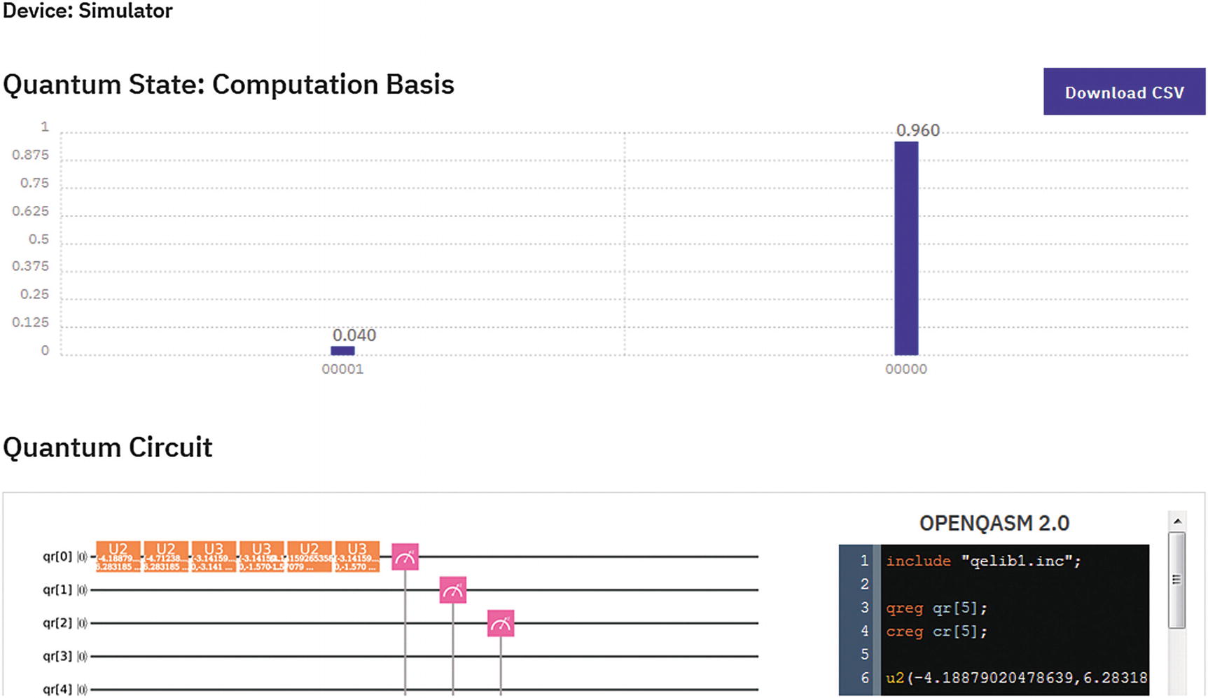
Note that quantum computers are probabilistic machines; therefore the definite state of the qubit cannot be known (it is forbidden by quantum mechanics). Thus all we get is the probability that the qubit is in state 0 or 1. For the simple quantum number generator on qubit zero h q[0] in the preceding paragraph, we can use the probability of state 1 as our random number. This can be seen as a neat graph shown by the IBM Q Experience Composer when the results are collected after the assembly code executes as shown in Figure 4-9.

You have taken the first step in this new career as a quantum programmer in the cloud. By using the high-level Python SDK and powerful quantum assembly engine, experiments can be run in the awesome IBM Q Experience platform. These skills will be valuable in a few years when quantum computers start to join the data center. In the next chapter, we take things to the next level with a set of algorithms that show the almost magical powers of quantum mechanics when applied to computation. So read on.

Previous Chapter

3. Enter the IBM Q Experience: A One-of-a-Kind Platform for Quantum Computing in the Cloud

Next Chapter

5. Start Your Engines: From Quantum Random Numbers to Teleportation, Pit Stop at Super Dense Coding

Table of Contents for Practical Quantum Computing for Developers: Programming Quantum Rigs in the Cloud using Python, Quantum Assembly Language and IBM QExperience

4. QISKit, Awesome SDK for Quantum Programming in Python

Installing the QISKit

Setting Up in Windows

Setting Up in Linux CentOS

Tip

Step 1: Prepare Your System

Step 2: Install Python 3

Step 3: Don’t Disturb Others – Set Up a Virtual Environment

Tip

Step 4: Install QISKit

Tip

Qubit 101: It’s Just Basic Algebra

Algebraic Representation of a Quantum Bit

Tip

Dirac’s Ket Notation

Tip

Superposition Is Just a Fancy Word

Tip

Ket Notation Too Weird? Use Vectors Instead

Changing the State of a Qubit with Quantum Gates

NOT Gate (Pauli X)

Truly Quantum: Superpositions with the Hadamard Gate

Measurement of a Quantum State Is Trickier Than You Think

Generalized Single-Qubit Gates

Tip

Unitary Matrices Are Good for Quantum Gates

Other Single-Qubit Gates

Qubit Entanglement with the Controlled NOT Gate

Tip

Universal Quantum Computation Delivers Shortcuts over Classical Computation

Your First Quantum Program

Tip

SDK Internals: Circuit Compilation and QASM

Circuit Compilation

Note

Execution Results

Tip

Assembly Code

Tip

QISKit Local Simulators

Running in the Local C++ simulator

Tip

Running in a Remote Simulator

Tip

And the Fastest Simulator Is Comparing Execution Times

Running in a Real Quantum Device

Tip

Note

Quantum Circuit for the Composer

Execution via Your Favorite REST Client

Tip

Run via the Jobs API

Tip

Tip

Run via the Execute API

Tip

Tip

Quantum Assembly: The Power Behind the Scenes

Tip

Table of Contents for
Practical Quantum Computing for Developers: Programming Quantum Rigs in the Cloud using Python, Quantum Assembly Language and IBM QExperience