This chapter takes you through a journey about three remarkable information processing capabilities of quantum systems. We start with one of the simplest procedures by exploring the fundamentally random nature of quantum mechanics as a source of true randomness. Next, the chapter looks at perhaps two exuberant but related procedures called super dense coding and quantum teleportation. In super dense coding, you will learn how it is possible to send 2 classical bits of information using a single qubit. In quantum teleportation, you will learn how the quantum state of a qubit can be recreated by a hybrid classical-quantum information transfer procedure. All algorithms include circuit design for the IBM Q Experience Composer as well as Python and QASM code. Results will be gathered for display and analysis, so let’s get started.
Quantum Random Number Generation
In this section you will learn how the probabilistic nature of a quantum computer can be exploited to generate random bits or numbers using the Hadamard gate.
Random Bit Generation Using the Hadamard Gate
![$$ H=\frac{1}{\sqrt{2}}\left[\begin{array}{cc}1& 1\\ {}1& -1\end{array}\right] $$](../images/469026_1_En_5_Chapter/469026_1_En_5_Chapter_TeX_Equa.png)
To understand better how this matrix puts a qubit in superposition, consider the geometrical representation of a single qubit:
![$$ \mid 0\Big\rangle =\left[\begin{array}{c}1\\ {}0\end{array}\right] $$](../images/469026_1_En_5_Chapter/469026_1_En_5_Chapter_TeX_IEq1.png) and
and ![$$ \mid 1\Big\rangle =\left[\begin{array}{c}0\\ {}1\end{array}\right] $$](../images/469026_1_En_5_Chapter/469026_1_En_5_Chapter_TeX_IEq2.png) . Remember from the previous chapter that a ket is simply a unitary vector (a vector of length 1). Thus the general (or superposition) state is then defined by the unitary vector ψ = α|0⟩+β|1⟩ where α and β are complex coefficients. Applying H to the basis states gives
. Remember from the previous chapter that a ket is simply a unitary vector (a vector of length 1). Thus the general (or superposition) state is then defined by the unitary vector ψ = α|0⟩+β|1⟩ where α and β are complex coefficients. Applying H to the basis states gives![$$ H\mid 0\Big\rangle =\frac{1}{\sqrt{2}}\left[\begin{array}{cc}1& 1\\ {}1& -1\end{array}\right]\left[\begin{array}{c}1\\ {}0\end{array}\right]=\frac{1}{\sqrt{2}}\left[\begin{array}{c}1\\ {}1\end{array}\right]=\frac{1}{\sqrt{2}}\left(\left[\begin{array}{c}1\\ {}0\end{array}\right]+\left[\begin{array}{c}0\\ {}1\end{array}\right]\right)=\frac{\left|0\Big\rangle +|1\right\rangle }{\sqrt{2}} $$](../images/469026_1_En_5_Chapter/469026_1_En_5_Chapter_TeX_Equb.png)
![$$ H\mid 1\Big\rangle =\frac{1}{\sqrt{2}}\left[\begin{array}{cc}1& 1\\ {}1& -1\end{array}\right]\left[\begin{array}{c}0\\ {}1\end{array}\right]=\frac{1}{\sqrt{2}}\left[\begin{array}{c}1\\ {}-1\end{array}\right]=\frac{1}{\sqrt{2}}\left(\left[\begin{array}{c}1\\ {}0\end{array}\right]-\left[\begin{array}{c}0\\ {}1\end{array}\right]\right)=\frac{\left|0\Big\rangle -|1\right\rangle }{\sqrt{2}} $$](../images/469026_1_En_5_Chapter/469026_1_En_5_Chapter_TeX_Equc.png)

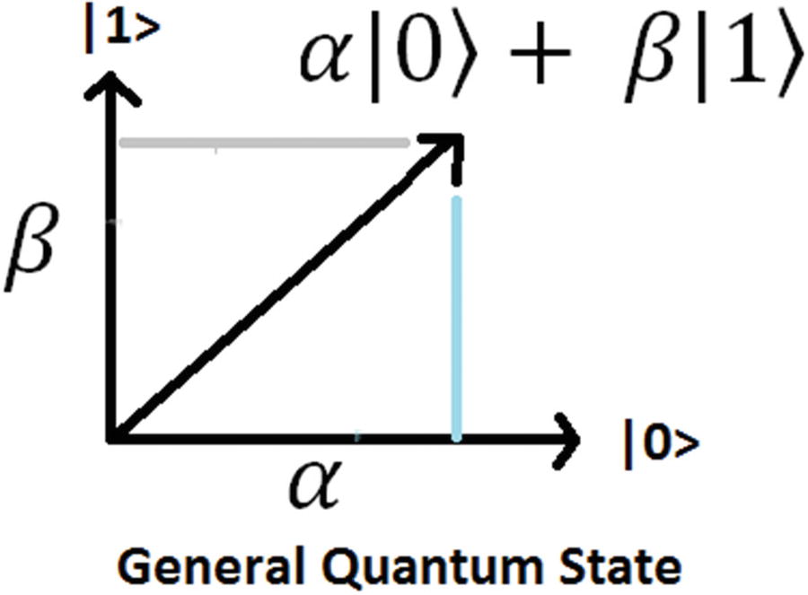
Geometrical representation of the general (superimposed) state ψ of a qubit
Tip
Quantum mechanics says that we can’t predict with certainty the values of coefficients α and β in the preceding basis states, even given complete knowledge of the laws of physics or a particle’s initial conditions. The best we can do is to calculate a probability.
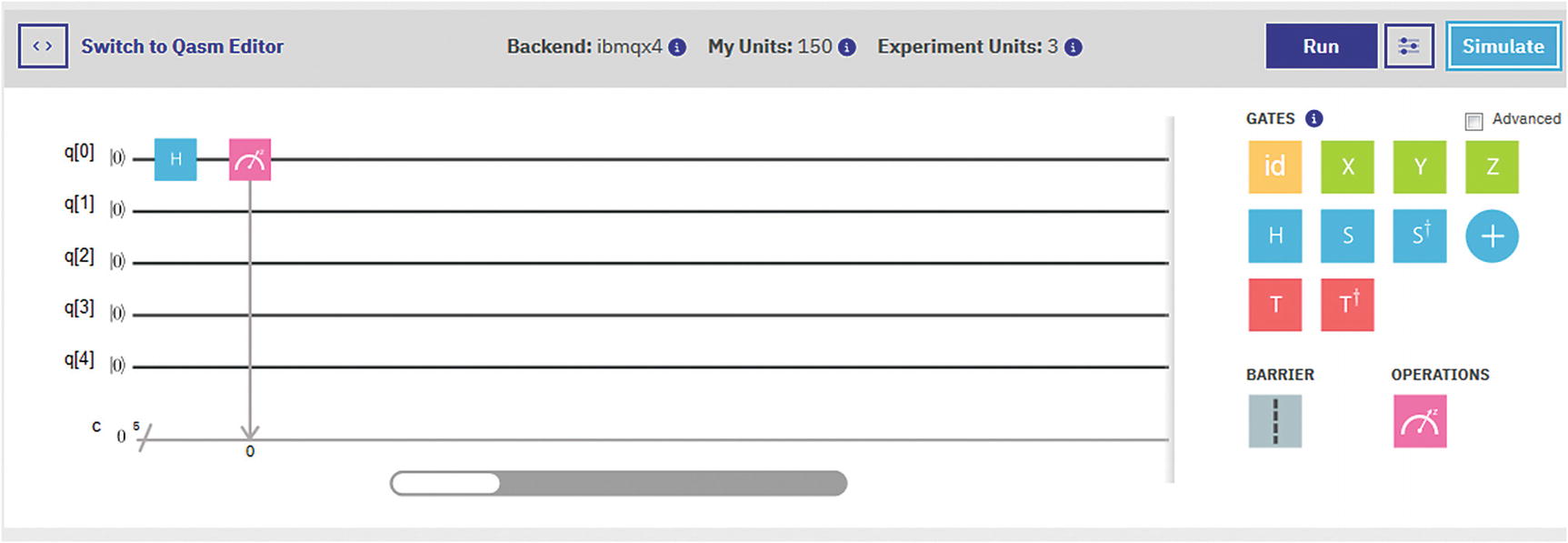
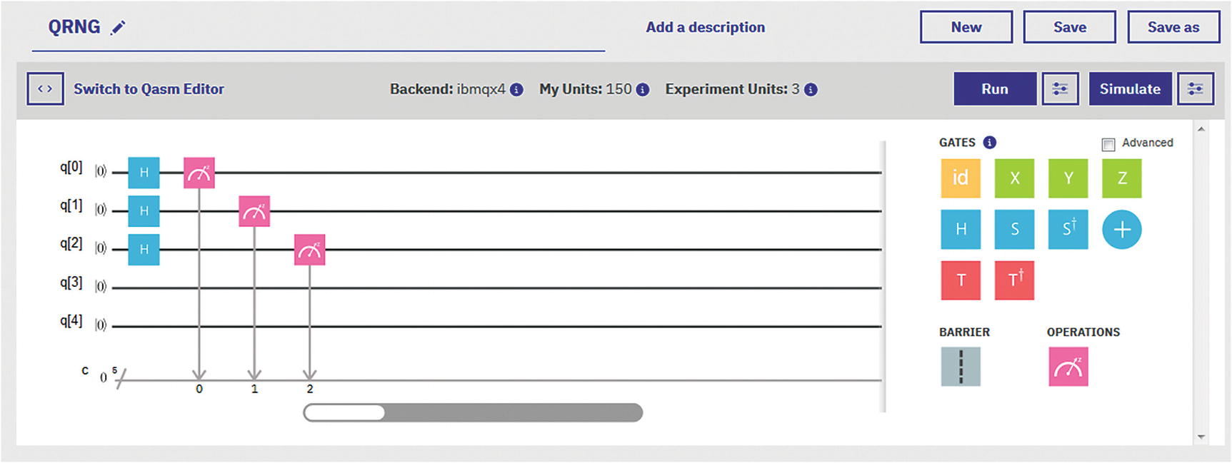
Circuit for a random bit generation
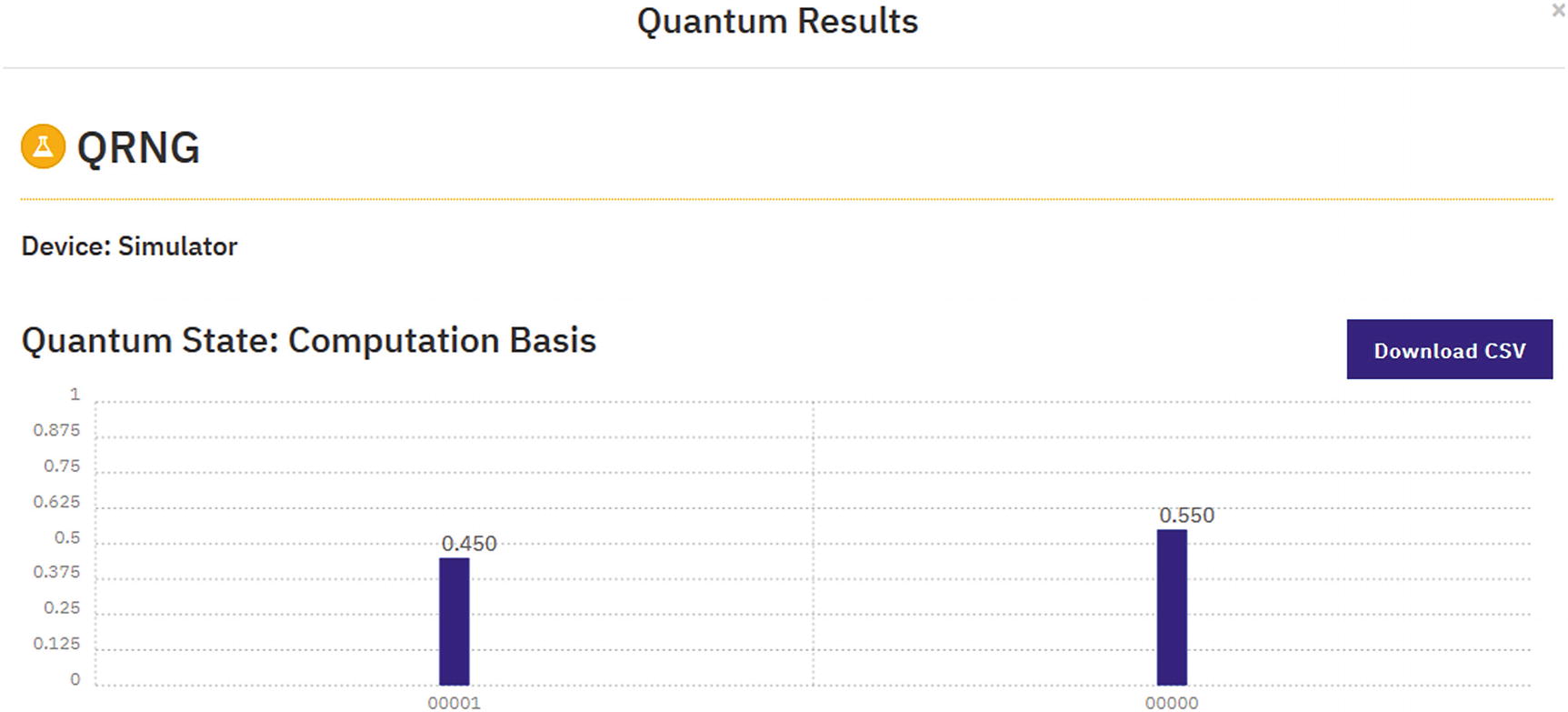
Execution results for circuit in Figure 5-2
Line 12 defines the function qrng to create a circuit using n qubits.
Using the QISKitAPI, lines 15-21 create a QuantumProgram with n qubits and n classical registers to store the measurements.
A Hadamard gate is applied to all qubits, then a measurement is performed on each, and finally the result is stored in classical register n (lines 30-35).
The circuit is compiled to run in the Q Experience remote simulator by using the system call set_api(API-TOKEN, URL). Note that you will need your configuration descriptor with the API token and end point URL. The circuit gets executed and the result counts are collected (lines 40-51).
- Finally to generate random bits, look at the outcome counts. For example, given the results {'100': 133, '101': 134, '011': 131, '110': 125, '001': 109, '111': 128, '010': 138, '000': 126}. For each outcome, if the count is greater than the average probability, then you get a 1, else you get a 0. The average probability is calculated by dividing the number of shots (1024 in this case) by the number of outcomes (2x where x is the number of qubits (default is 3) – 1024/8 = 128). Thus, for the preceding results
133
1
134
1
11100010 = 226
131
1
125
0
109
0
128
0
138
1
126
0
Quantum Program to Generate n Random Numbers of 2x Bits
Caution
Before executing any program, always make sure your configuration is correct including a valid API token and end point URL. This is a major source of headaches. Remember that your program will fail if you miss this crucial step.
Q Experience circuit for Listing 5-1
Let’s gather some data from multiple runs and put the results to the test.
Putting Randomness Results to the Test
Linux provides a neat program called ent (short for entropy) which is called a pseudorandom number sequence test program.1 We can use this command to test the numbers generated in the previous section.
Tip
Windows users – a Windows 32 binary is available for download from the project site. A binary is also included in the source for this chapter under Workspace\Ch05\ent.exe.
Randomness Test Results from Various Sources Gathered by ENT1
Source | Chi-square percentage |
|---|---|
UNIX rand() | 99.9% for 500,000 samples (bad) |
Improved UNIX generator by Park & Miller | 97.53% for 500,000 samples (better) |
HotBits: random numbers, generated by radioactive decay | 40.98% for 500,000 samples (the best) |
The preceding table clearly shows that UNIX rand() shouldn’t be trusted for random number generation. If you need lots of truly random numbers (e.g., to generate encryption keys), use a quantum source such as HotBits. All in all, the purpose of this section has been to get your feet wet with a simple quantum circuit for random number generation. The next section takes things to the next level with the bizarre quantum data transfer protocol dubbed super dense coding.
Super Dense Coding
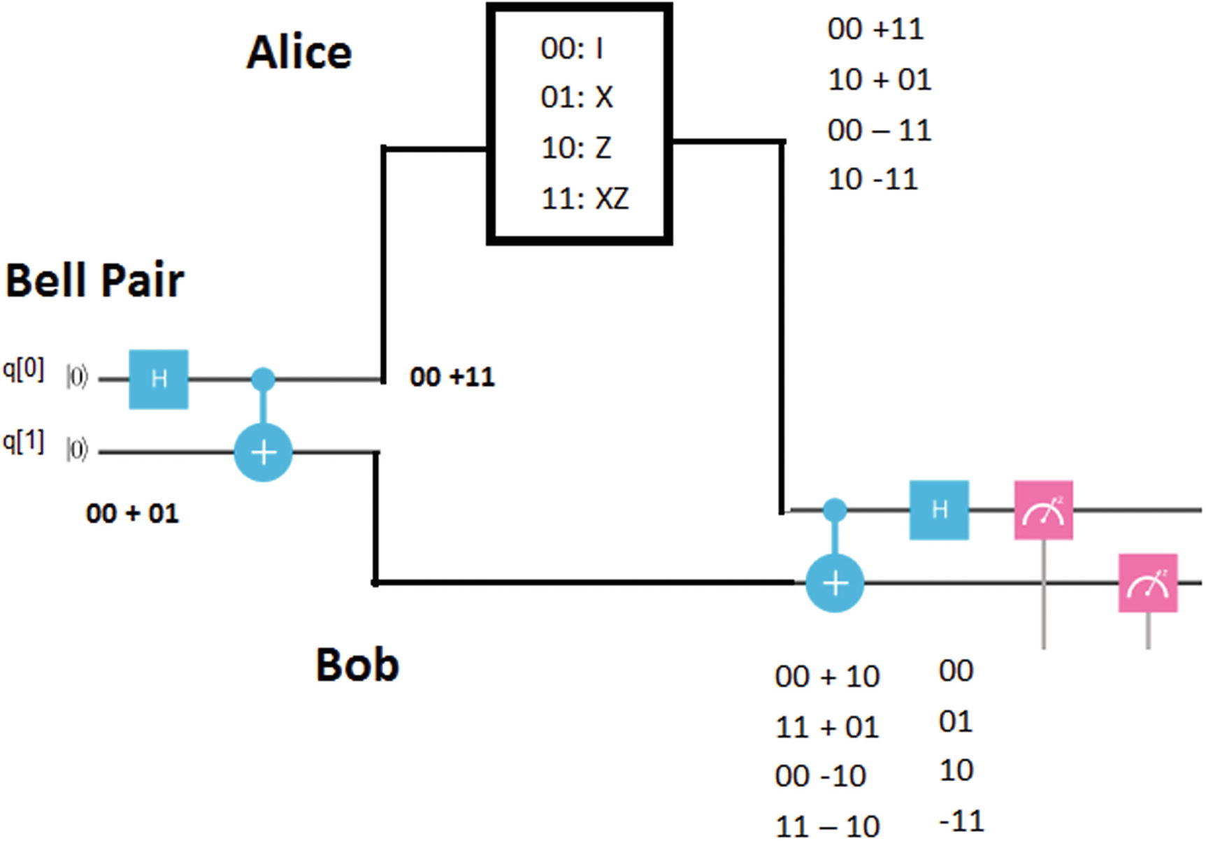
Super dense coding protocol
- 1.The process starts with a third party (Eve) generating what is called a Bell Pair. Eve starts with 2 qubits in the basis state |0>. She applies a Hadamard gate to the first qubit to create superposition. It then applies a CNOT gate using the first qubit as the control (dot) and the second as the target (+). This results in the states shown in Table 5-2.Table 5-2
Bell Pair States
Gate
Outcome states
Details
H
∣00⟩ → ∣ 00⟩+ ∣ 10⟩
When the H gate is applied to the first qubit, it enters superposition; thus we get the states 00 + 10 where the second qubit remains as 0. Note that the square root (2) from the Hadamard matrix has been omitted for simplicity.
CNOT
∣00⟩+ ∣ 10⟩ → ∣ 00⟩+ ∣ 11⟩
The CNOT gate entangles both qubits. In particular, it flips the target (+) if the control (.) is 1, else it leaves intact. Thus we flip the second qubit if the first is 1 resulting in 00 + 11.
- 2.In the second step of the process, the first qubit is sent to Alice and the second to Bob. Note that Alice and Bob may be in remote places. The goal of the protocol is for Alice to send 2 classical bits of information to Bob using her qubit. But before she does, she needs to apply a set of quantum rules (or gates) to her qubit depending on the 2 bits of information she wants to send. (See Table 5-3.)Table 5-3
Encoding Rules for Super Dense Coding
Rules
Outcome States
00: I (identity gate)
01: X
10: Z
11: ZX
I(00+11) = 00 + 11
X(00+11) = 10 + 01
Z(00+11) = 00 – 11
ZX(00+11) = 10 – 11
- 3.
Thus if she sends a 00, she does nothing to her qubit (applies the identity gate). If she sends a 01, then she applies the X gate (or bit flip). For a 10 she applies the Z gate. Note that the Z gate flips the sign (phase) of the qubit if the qubit is 1. Thus Z ∣ 0⟩ = |0⟩, Z| 1⟩ = − ∣ 1⟩. Finally, if she sends 11, then she applies gates XZ to her qubit. Alice then sends her qubit to Bob for the final step in the process.
- 4.Bob receives Alice’s qubit (qubit 0) and uses his qubit to reverse the process of the Bell state created by Eve. That is, he applies the CNOT gate to the first qubit followed by the Hadamard gate (H) and finally performs a measurement in both qubits to extract the 2 classical bits encoded in Alice’s qubit (see Table 5-4).Table 5-4
Qubit States After Recovery
Gate
Outcome States
Details
CNOT
00 +10
11 + 01
00 – 10
11 – 10
We start with Alice’s states from step 2:
00 + 11
10 + 01
00 – 11
10 – 11
The CNOT gate flips the second qubit if the first is 1 resulting in the states in column #2.
H
00
01
10
–11
Applying the Hadamard to the first qubit in the last row results in the outcomes in column #2. When Bob performs measurements in the computational basis states, he ends up with four possible outcomes with probability 1 each. These outcomes match what Alice meant to send in step 2 column #1. Note that the last outcome has a negative sign. Nevertheless, because the probability is calculated as the amplitude squared, the –1 becomes 1 which is correct.
Let’s put all this together in a circuit within the IBM Q Experience Composer.
Circuit for Composer
The circuit begins by creating a Bell Pair; that is, it puts qubit[0] in superposition (using the Hadamard gate) and then entangles it with qubit[1] via the CNOT gate.
The next two gates represent Alice’s encoding rules. Remember that she applies the identity (nothing) to encode bits 00, X to encode 01, Z to encode 10, and ZX to encode 11. In this particular case, the encoded bits are 11. This is shown left of the barrier symbol in Figure 5-6. Note that the barrier will block execution until all gates are consumed by both qubits.
To the right side of the barrier symbol, there is Bob’s protocol. He basically does the reverse operation as Alice’s. He applies the CNOT gate and then a Hadamard gate on the qubits. Finally a measurement is performed on both qubits to extract the 2 encoded classical bits.
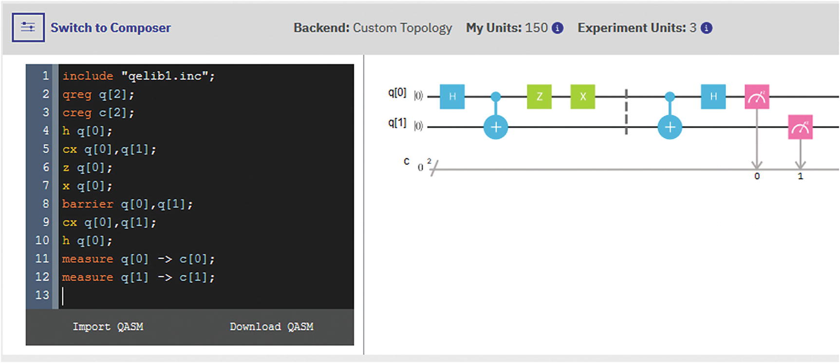
Superdense circuit for Q Experience
Run the preceding circuit in the simulator, and the result should be a bar graph with the probability for outcome 11 very close or equal to 1. This result should match the result obtained in the next section using a Python script.
Running Remotely Using Python
Lines 17–19 create 2 qubits and two classical registers to hold the outcomes.
Next the superdense circuit is created with the entangled Bell Pair (lines 22–14).
Alice encodes 11 by applying the ZX gates. Optionally, comment any of these statements to encode a different pair, and then make sure the result matches Alice’s encoding scheme (lines 32–35).
Bob reverses Alice’s operation and measures the qubits (lines 38–41).
Finally, the circuit gets executed in the remote simulator (ibmq_qasm_simulator) and the results displayed using Python’s excellent plotting support.
Super Dense Coding Python Script
Let’s look at the results of a single run of Listing 5-2 in the next section.
Looking at the Results
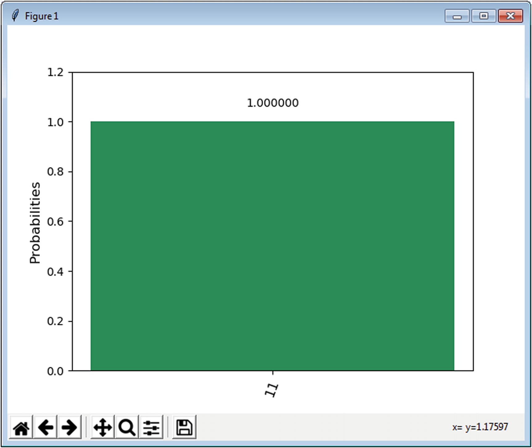
Super dense coding plot result
Thus super dense coding provides the means to encode 2 classical bits in a single qubit. Note that it is worth mentioning that quantum computation states that it is not possible to store more than a single classical bit per qubit which seems to contradict what has been shown in this protocol. As a matter of fact, there is no contradiction. The protocol works because Alice’s and Bob’s qubits are entangled via a Bell Pair. This allows for sending 2 classical bits in Alice’s entangled qubit. All in all, you can store at most 2 classical bits per qubit provided that your qubit is entangled to another via a Bell Pair.
In general terms, this protocol could be interpreted as a set of modularized abstractions: a Bell Pair generator module to create 2 entangled qubits, followed by an information encoder module which applies Alice’s rules to encode the 2 classical bits of information. Finally, a decoder module extracts the classical bits from the qubits provided by the Bell Pair as well as the encoder module (sort of a quantum zip/unzip tool if you will). Super dense coding provides a high-level picture for quantum information processing and will help you understand the next item in this chapter: quantum teleportation.
Tip
This simple protocol was developed in 1992 by physicist Charles Bennett almost 70 years after the discovery of quantum mechanics. Despite its relative simplicity, it is not an obvious procedure, and remarkable things can be learned by studying it in depth.
Quantum Teleportation
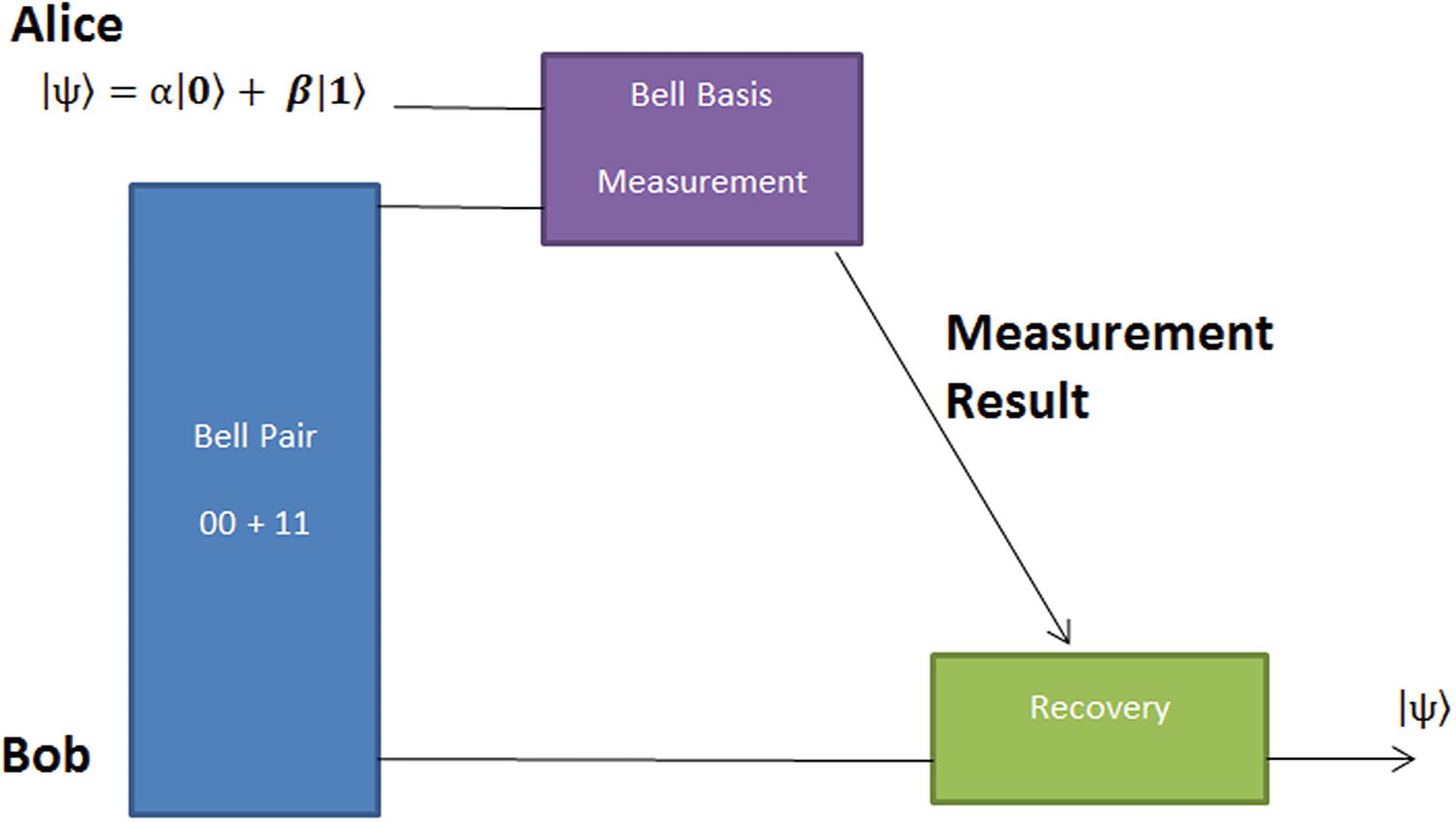
Quantum teleportation workflow
- 1.
Alice and Bob start by sharing a Bell Pair of entangled qubits. One goes to Alice and the other goes to Bob at separate remote locations. Imagine that the Bell Pair is prepared by a third party (Eve).
- 2.
Alice prepares her qubit to be teleported in state |ψ⟩ = α|0⟩+β ∣ 1⟩. She then performs a Bell basis measurement of her qubit and the entangled qubit from the Bell Pair provided by Eve. Alice then sends the measurement result by classical means to Bob.
- 3.
At this point there is a posterior state for Bob’s qubit as a function of the measurement performed by Alice. This is the key to understanding the procedure; remember that both share an entangled qubit. Thus we’ll see how Bob, by applying the appropriate quantum gate, can recover the original state ψ created by Alice.
B0 = 00 + 11 B1 = 10 + 01 B2 = 00 – 11 B3 = 10 – 01 | 00 = B0 – B1 01 = B1 – B3 10 = B1 – B3 11 = B0 – B2 |
Quantum Teleportation Recovery
Bell State | Posterior State | Bob’s Recovery Operation |
|---|---|---|
B0 | α0 + β1 | ψ |
B1 | α1 + β0 | Xψ |
B2 | α0 – β1 | Zψ |
B3 | –α1+ β0 | ZXψ |
All in all, the quantum teleportation protocol provides the means to recover the state ψ of any qubit by sharing an entangled Bell Pair between two remote parties, hence the name teleportation. Now let’s build a circuit for this protocol, run it in the simulator, and finally look at the results.
Circuit for Composer
The gates left of the barrier symbol (the dotted line) represent the Bell Pair prepared by the third party (Eve): qubits 1 and 2.
Alice prepares her qubit (0) to a given state ψ. The actual value of ψ is irrelevant as it will be recovered by Bob at the final stage of the process. Alice receives qubit[1] from Eve, and qubit[2] goes to Bob.
Alice performs a measurement on her qubits [0,1] (shown to the right of the dotted line) and sends the results by classical means to Bob.
Bob applies the recovery rules to his qubit (2) mentioned in the previous section depending on the outcomes sent by Alice. Finally, after a measurement of qubit[2], Bob recovers the state ψ originally created by Alice. All this is made possible by the fact that Alice and Bob share an entangled pair of qubits which makes the whole thing work.
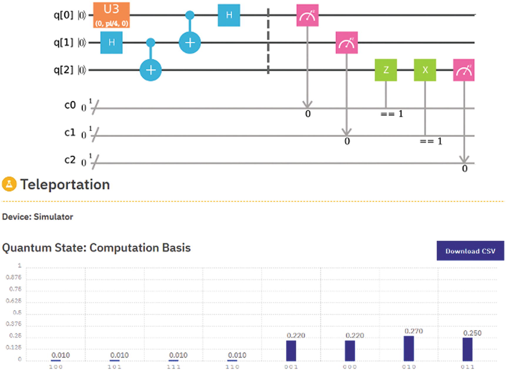
Quantum teleportation circuit for the Composer
Of course, the execution results in Figure 5-9 need to be massaged to verify that Bob’s ψ matches Alice’s. The best way to do this is to use a Python script. In the next section, we’ll run the same circuit remotely and look at the results to verify the protocol works.
Running Remotely Using Python
Three qubits are created to be shared by both parties: Alice and Bob, plus three classical registers (c0, c1, c2) to store Alice’s results (lines 20–23).
The Bell Pair is prepared by Eve by applying a Hadamard gate (H) followed by a controlled NOT (CNOT) gate in qubits 1 and 2 (lines 35–37).
Alice prepares her state ψ on qubit 0 by rotating on the Y-axis by π/4 radians (line 32).
Alice now entangles her qubit[0] with the Bell Pair qubit given to her, qubit[1], to entangle them. She then performs a measurement in both and stores the outcomes in classical registers 0, 1 (lines 35–41).
Now its Bob’s turn: He applies a Z or X gate on his qubit (2) depending on the outcomes sent by Alice – if classical register 0 is 1, then he applies a Z gate. If classical register 1 is 1, then he applies an X gate. Then he measures his qubit and stores the outcome in classical register 2 (lines 47–50).
The program is executed in the remote simulator (ibmq_qasm_simulator) and the results collected for display and verification (lines 58–79).
Tip
The source for this program is included in the book source under Workspace\Ch05\p05-teleport.py.
Python Script for Quantum Teleportation
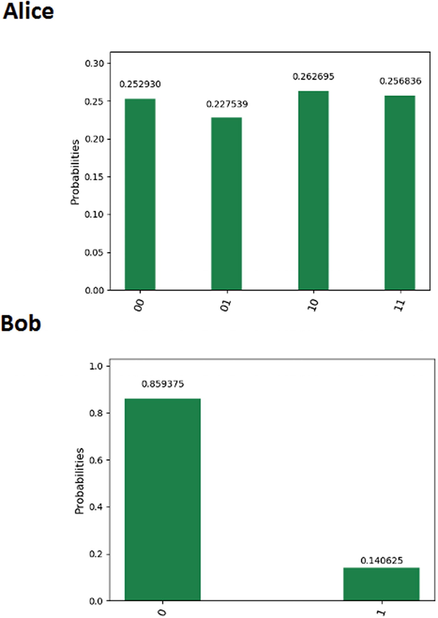
Probability results for Alice and Bob measurements
So what does this all mean? And how do we know that the state ψ has been recovered by Bob? Let’s look at these results in more detail.
Looking at the Results
Probability Results for the Quantum Teleportation Experiment
Row | Outcome | Count | Probability | Alice | Probability Sum | |||
|---|---|---|---|---|---|---|---|---|
0 | Alice(00) | Bob(0) | 0 0 0 | 206 | 0.201171875 | 0 0 | 0.237304688 | |
1 | Alice(01) | Bob(0) | 0 0 1 | 200 | 0.1953125 | 1 0 | 0.239257813 | |
2 | Alice(10) | Bob(0) | 0 1 0 | 230 | 0.224609375 | 0 1 | 0.271484375 | |
3 | Alice(11) | Bob(0) | 0 1 1 | 215 | 0.209960938 | 1 1 | 0.251953125 | |
4 | Alice(00) | Bob(1) | 1 0 0 | 37 | 0.036132813 | |||
5 | Alice(01) | Bob(1) | 1 0 1 | 45 | 0.043945313 | Bob | ||
6 | Alice(10) | Bob(1) | 1 1 0 | 48 | 0.046875 | 0 | 0.831054688 | |
7 | Alice(11) | Bob(1) | 1 1 1 | 43 | 0.041992188 | 1 | 0.168945313 |
Bob | |
0 | 0.20 + 0.19 + 0.22 + 0.20 = 0.83 |
1 | 0.036 + 0.043 + 0.046 + 0.041 = 0.168 |

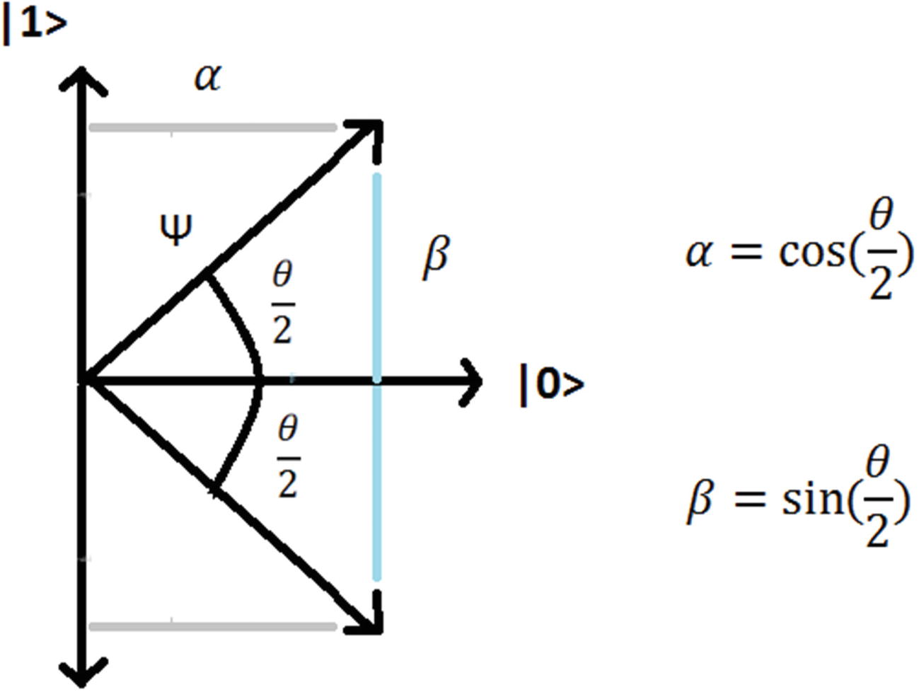
Superimposed state for Alice’s ψ


Probability (α) = |cos(π/8)|2 = 0.85
Probability (β) = |sin(π/8)|2 = 0.14
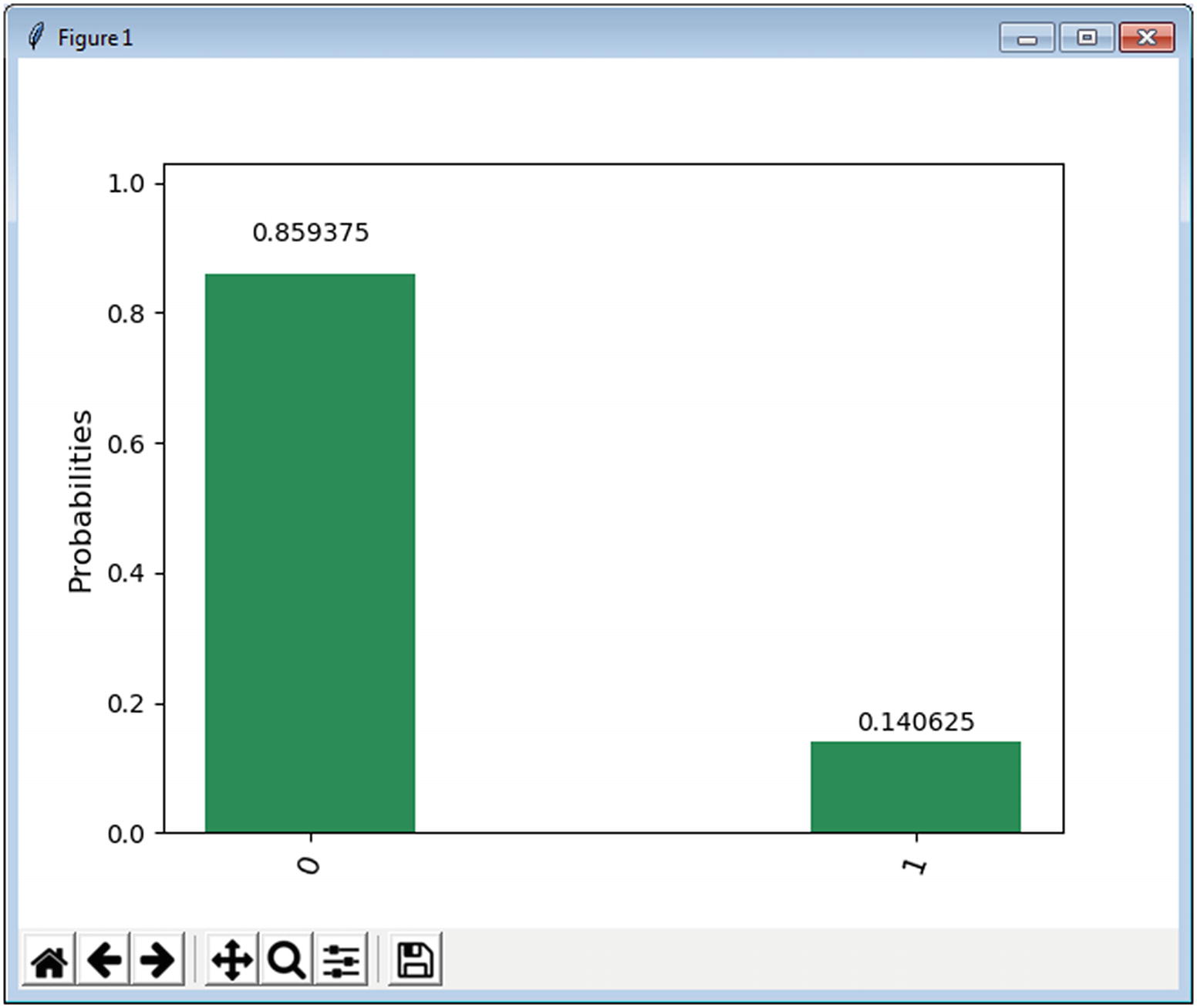
Teleportation results for Bob
You have taken the first step to understand the remarkable information processing capabilities of quantum systems. We started with a simple procedure to exploit the source of true randomness intrinsic to quantum mechanics to generate random numbers. We also explored two bizarre protocols: super dense coding to encode classical information and quantum teleportation to recover the state of a qubit by a remote party. These protocols have been described using circuits for the IBM Q Experience as well as Python scripts for remote execution in a simulator or real quantum device. Results have been collected and explained to understand what goes on behind the scenes. The next chapter explores the lighter side of quantum computing, by having fun creating a simple game using quantum gates: a needed break before we get to heavy stuff in later chapters.