In this chapter we take a look at quantum computing in the cloud with IBM Q Experience: the first platform of its kind. The chapter starts with an overview of the Composer, the web console used to visually create circuits, submit experiments, explore hardware devices, and more. Next, you will learn how to create your first experiment and submit it to the simulator or real quantum device. IBM Q Experience features a powerful REST API to control the life cycle of the experiment, and this chapter will show you how with detailed descriptions of the end points and request parameters. Finally, the chapter ends with a practical implementation of the official Python library (dubbed IBMQuantumExperience) for Node JS. This custom Node JS library will put your asynchronous Javascript and REST API skills to the test. Let’s get started.
IBM has certainly taken an early lead in the race for quantum computing in the cloud. They came up with a really cool platform to run experiments remotely called the Q Experience. But is it just me or the names of these tools make a lot of analogies to music theory? Check this out: the visual editor used to create quantum circuits is called the Composer. Not weird enough? The quantum circuits built with the editor are called scores (as in a music score), not to mention that visually the editor looks a lot like the written score of a musical composition. I say this because I’ve been playing the classical guitar for a long time and had an eerie familiarity with a guitar score the first time I looked at the Composer (with the gates looking a lot like music notes). Still think I am crazy? The platform is called the Q Experience; have you ever heard about the Jimi Hendrix Experience? Perhaps the Composer is the score workbook where you will create a great masterpiece for the rest of us to enjoy. Quantum computing does have the power to transform the status quo.
Getting Your Feet Wet with IBM Q Experience
Create an account in https://quantumexperience.ng.bluemix.net/qx/experience . You will need an email, wait for the approval, and confirm.
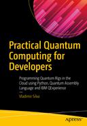
Log in to the web console and navigate to the Composer tab on the top (see Figure 3-1).
IBM Q Experience main window
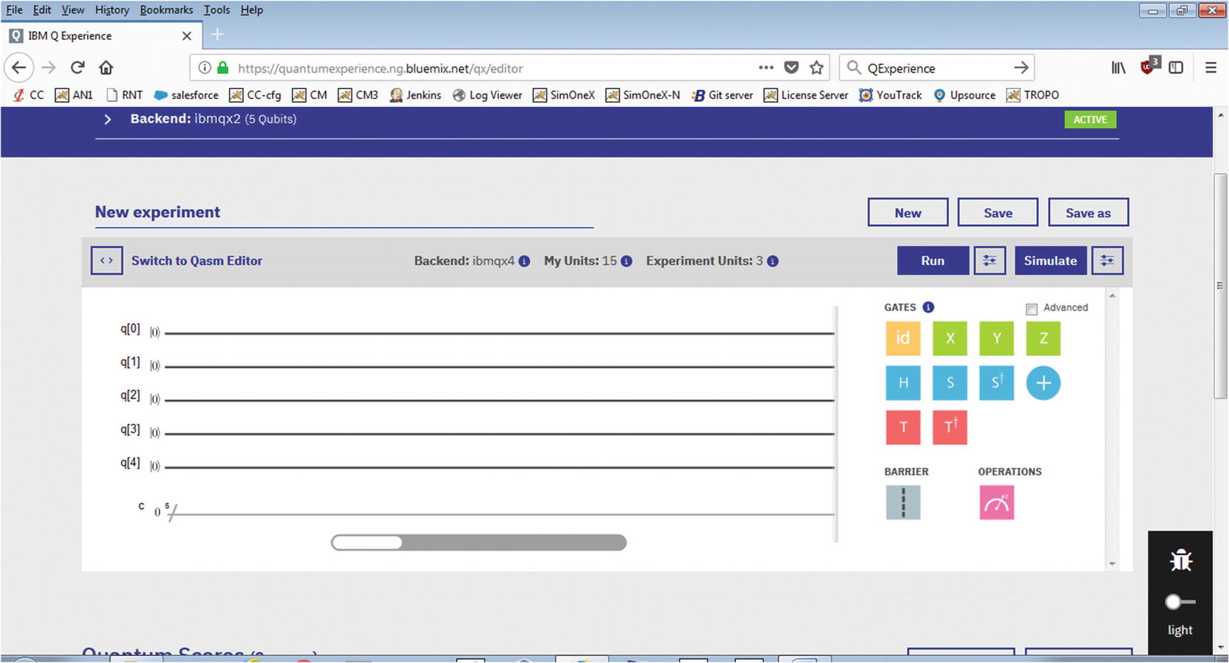
Quantum Composer
Experiment Composer
On the left side of the histogram, we see 5 qubits available from processor ibmqx4. They are all initialized to the ground state |0>. The line at the bottom is the measurement line where the results of the circuit will be collected. Remember that measurement should be the last thing done in the circuit as all gate operations execute in parallel and in superimposed states.
On the right side, we have the quantum gates. Drag gates into the histogram location of a specific qubit to start building a circuit.
Let’s look at the gates and their meaning.
Quantum Gates
Quantum Gates for IBM Q Experience
Gate | Description |
|---|---|
Pauli X
| It rotates the qubit 180 degrees in the X-axis. Maps |0> to |1> and |1> to |0>. Also it is known as the bit flip or NOT gate. It is represented by the matrix:
|
Pauli Y
| It rotates around the Y-axis of the Bloch sphere by π radians. It is represented by the Pauli matrix:
where |
Pauli Z
| It rotates around the Z-axis of the Bloch sphere by π radians. It is represented by the Pauli matrix:
|
Hadamard
| It represents a rotation of π on the axis • |0> to • |1> to This gate is required to make superpositions. |
Phase
| It has the property that it maps X→Y and Z→Z. This gate extends H to make complex superpositions. |
Transposed conjugate of S
| It maps X→-Y and Z→Z. |
Controlled NOT (CNOT)
| This is a 2-qubit gate that flips the target qubit (applies Pauli X) if the control is in state 1. This gate is required to generate entanglement. |
Phase
| The
|
Transposed conjugate of T or T-dagger
| Represented by the matrix:
|
Barrier
| It prevents transformations across its source line. |
Measurement
| The measurement gate takes a qubit in a superposition of states as input and spits either a 0 or 1. Furthermore, the output is not random. There is a probability of a 0 or 1 as output which depends on the original state of the qubit. |
Conditional
| Conditionally apply a quantum operation. |
Physical partial rotation (U gates)
| U1: It is a one parameter single-qubit phase gate with zero duration. U2: It is a two-parameter single-qubit gate with duration of one unit of gate time. U3: It is a three-parameter single-qubit gate with duration of two units of gate time. |
Identity
| The identity gate performs an idle operation on the qubit for a time equal to one unit of time. |

![$$ X=\left[\begin{array}{cc}0& 1\\ {}1& 0\end{array}\right] $$](../images/469026_1_En_3_Chapter/469026_1_En_3_Chapter_TeX_IEq1.png)

![$$ Y=\left[\begin{array}{cc}0& -i\\ {}-i& 0\end{array}\right] $$](../images/469026_1_En_3_Chapter/469026_1_En_3_Chapter_TeX_IEq2.png)


![$$ Z=\left[\begin{array}{cc}1& 0\\ {}0& -1\end{array}\right] $$](../images/469026_1_En_3_Chapter/469026_1_En_3_Chapter_TeX_IEq4.png)


![$$ \sqrt{S}=\left[\begin{array}{cccc}1& 0& 0& 0\\ {}0& 1/2\left(1+i\right)& 1/2\left(1-i\right)& 0\\ {}0& 1/2\left(1-i\right)& 1/2\left(1+i\right)& 0\\ {}0& 0& 0& 1\end{array}\right] $$](../images/469026_1_En_3_Chapter/469026_1_En_3_Chapter_TeX_IEq11.png)

![$$ \sqrt{S}=\left[\begin{array}{cccc}1& 0& 0& 0\\ {}0& 1/2\left(1-i\right)& 1/2\left(1+i\right)& 0\\ {}0& 1/2\left(1+i\right)& 1/2\left(1-i\right)& 0\\ {}0& 0& 0& 1\end{array}\right] $$](../images/469026_1_En_3_Chapter/469026_1_En_3_Chapter_TeX_IEq12.png)


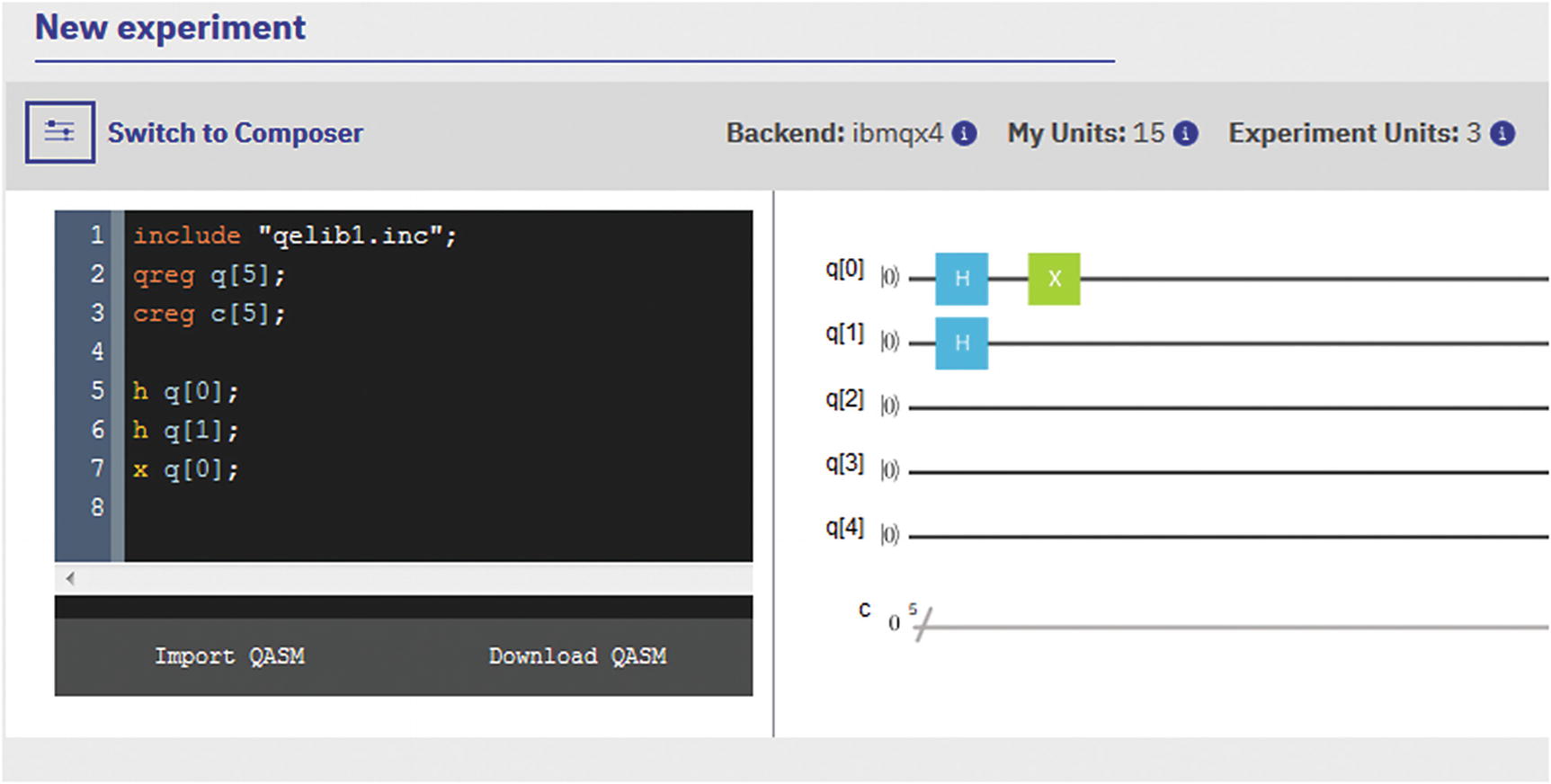
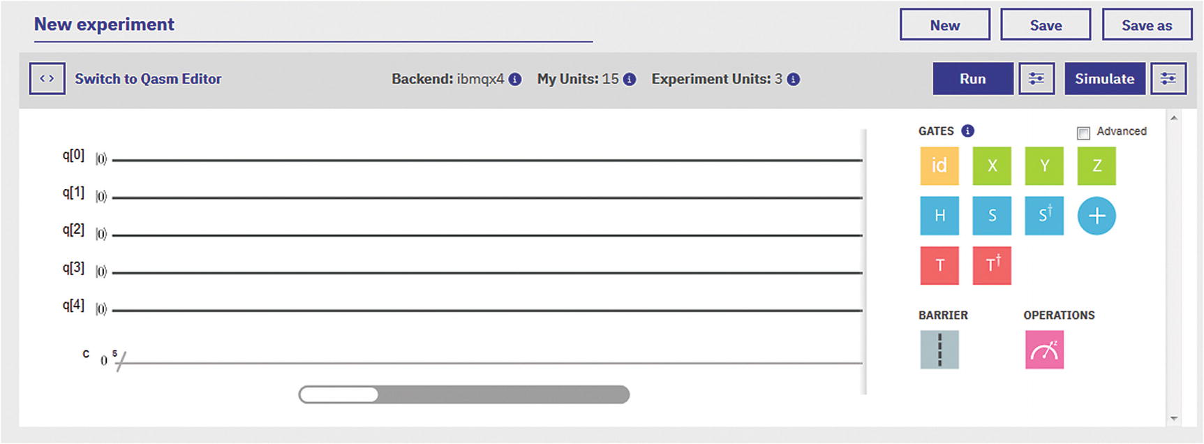
Experiment editor in QASM editor mode
Tip
QASM is the quantum assembly language, built on top of the OPENQASM platform, and it is used to implement experiments with low-depth quantum circuits. Even though assembler has become something of a lost art, some people may find its raw power more appealing than the Python SDK or even the visual editor.
Now let’s take a look at the various quantum processors available for use.
Quantum Backends Available for Use
Official List of Quantum Backends Available for IBM Q Experience Users
Name | Details |
|---|---|
Ibmqx2 | Code Name: Sparrow Qubits: 5 Online since January 24, 2017 |
Ibmqx4 | Code Name: Raven Qubits: 5 Online since September 25, 2017 |
Ibmqx3 | Code Name: Albatross Qubits: 16 Online since June 2017 |
Ibmqx5 | Code Name: Albatross Qubits: 16 Online since online September 28, 2017 This device is reconfigured version of ibmqx3. |
Table 3-2 shows the official list of processors available for use at the time of this writing, but there is a much interesting way to get an updated list of available machines in real time using the excellent REST API. This API is described in more detail on the “Remote Access via the REST API” section in this chapter, but for now let’s demonstrate how to obtain an always up-to-date list of backends using the Available Backend List REST end point:
https://quantumexperience.ng.bluemix.net/api/Backends?access_token=ACCESS-TOKEN
Tip
To obtain an access token, see the section “Authentication via API Token” under “Remote Access via the REST API” of this chapter. Note that an API token is not the same as an access token. API tokens are used to execute quantum programs via the Python SDK. Access tokens are used to invoke the REST API.
HTTP Response from the Backend Information REST API Call
- Extra processors and simulators:
It looks like there are two remote simulators available for use (ibmqx_qasm_simulator, ibmqx_hpc_qasm_simulator) even though the official documentation mentions only one: ibmqx_qasm_simulator. This information can come in handy when testing complex circuits: more simulators are always a good thing.
Rumors of a 20-qubit processor have been swirling around for some time. There is even talk of an upcoming 50-qubit monster processor by the end of 2018. This list seems to confirm the 20-qubit machine at least. But don’t get excited just yet; this machine is only available for corporate customers.
- Besides the usual information such as machine name, version, status, number of qubits, and others, there are some terms we should be familiarized with:
- basisGates : These are the physical qubit gates of the processor. They are the foundation under which more complex logical gates can be constructed. Most of the processors in the list use u1, u2, u3, cx, id.
Gates u1, u2, u3 are called partial NOT gates and perform rotations on axes X, Y, Z by theta, phi, or lambda radians of a qubit.
Cx is called the controlled NOT gate (CNOT or CX). It acts on 2 qubits and performs the NOT operation on the second qubit only when the first qubit is |1> and otherwise leaves it unchanged.
Id is the identity gate which performs an idle operation on a qubit for one unit of time.
couplingMap: The coupling map defines interactions between individual qubits while retaining quantum coherence (or a pure state – imagine a peloton of soldiers breaking step when crossing an old bridge so that the amplitude of their feet hitting the ground does not add up and destroy the bridge). Qubit coupling is used to simplify quantum circuitry and allow the system to be broken up into smaller units.
Now back to the Composer for our first quantum composition.
Opus 1: Variations on Bell and GHZ States
Bell states: They demonstrate that physics are not described by local reality. This is what Einstein called spooky action at a distance.
GHZ states: Even stranger than Bell states, GHZ states (named after their creators: Greenberger-Horne-Zeilinger) are the 3-qubit generalization of the Bell states.
Let’s look at them in more detail.
Bell States and Spooky Action at a Distance
Bell states are the experimental test of the famous Bell inequalities. In 1964 Irish physicist John Bell proposed a way to put quantum entanglement (spooky action at a distance) to the test. He came up with a set of inequalities which have become incredibly important in the physics community. This set of inequalities is known as Bell’s theorem, and it goes something like this.
Permutations for Photon Polarizations at Three Angles
Count | A(0) | B(120) | C(240) | [AB] | [BC] | [AC] | Sum | Average |
|---|---|---|---|---|---|---|---|---|
1 | A+ | B+ | C+ | 1(++) | 1(++) | 1(++) | 3 | 1 |
2 | A+ | B+ | C– | 1(++) | 0 | 0 | 1 | 1/3 |
3 | A+ | B– | C+ | 0 | 0 | 1(++) | 1 | 1/3 |
4 | A+ | B– | C– | 0 | 1(−−) | 0 | 1 | 1/3 |
5 | A− | B+ | C+ | 0 | 1(++) | 0 | 1 | 1/3 |
6 | A− | B+ | C− | 0 | 0 | 1(−−) | 1 | 1/3 |
7 | A− | B− | C+ | 1(−−) | 0 | 0 | 1 | 1/3 |
8 | A− | B− | C− | 1(−−) | 1(−−) | 1(−−) | 3 | 1 |
Now Bell’s theorem asks: what is the probability that the polarization at any neighbor will be the same as the first? We also calculate the sum and average of the polarizations. Assuming realism is true, then by looking at Table 3-3, the answer to the question is the probability must be >= 1/3. This is what Bell’s inequality gives: a means to put this assertion to the test. Here is the incredible part: believe it or not, quantum mechanics violates Bell’s inequality giving probabilities less than 1/3. This was proven experimentally for the first time in 1982 French physicist Alain Aspect.
Tip
A more detailed description of Aspect’s experiment and Bell’s inequality is described in Chapter 1, EPR Paradox Defeated: Bohr Has the Last Laugh.


A | B | 1 |
A | B' | 0 |
A' | B | 0 |
A' | B' | 1 |
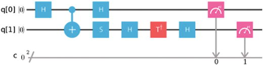
 , thus violating this inequality. This can be put to the test using four separate quantum circuits (one per measurement) with 2 qubits each. To simplify things, let measurements on Alice detector be A = Z and Aʹ = X, and Bob’s detector B = W and Bʹ = V (see Table 3-4). To begin the experiment, a basis Bell state must be constructed which matches the identity (see Figure 3-4):
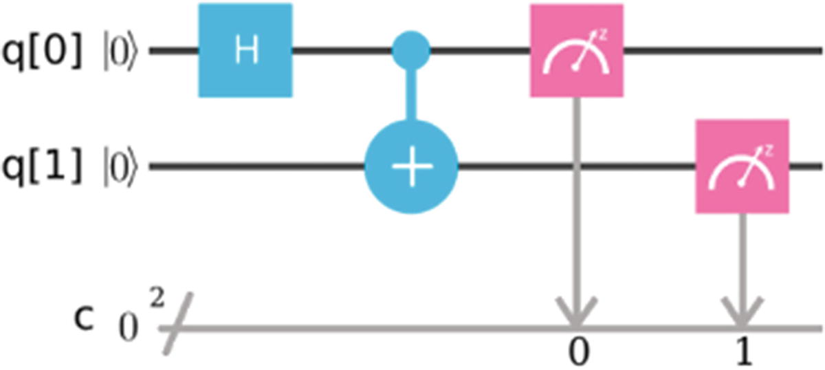
Basis Bell state
 . Next the CNOT gate flips the second qubit if the first is excited, making the state
  . This is the initial entangled state required for the four measurements in Table 3-4 (All reprints courtesy of International Business Machines Corporation, © International Business Machines Corporation).
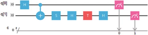
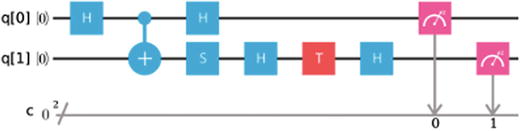
To rotate the measurement basis to the ZW axis, use the sequence of gates S-H-T-H.
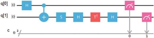
To rotate the measurement basis to the ZV axis, use the sequence of gates S-H-T’-H.
The XW and XV measurement is performed the same way as in the preceding text and the X via a Hadamard gate before a standard measurement.
Tip
Before performing the experiment in the Composer, make sure its topology (the number of qubits and target device) in the score is set to 2 over a simulator. Some topologies (like the 5 qubits in a real quantum device) do not support entanglement for qubits 0 and 1 giving errors at design. Note that the target device can be a real quantum processor or a simulator. All in all, as long as you use a simulator, you should be fine.
Quantum Circuits for Bell States
Bell state measurement | Result for 100 shots | ||||||||||
|---|---|---|---|---|---|---|---|---|---|---|---|
AB (ZW)
|
| ||||||||||
AB′ (ZV)
|
| ||||||||||
A′B (XW)
|
| ||||||||||
A′B′ (XV)
|
|

Compiled Results from the Bell Experiment
P(00) | P(11) | P(01) | P(10) | <AB> | |
|---|---|---|---|---|---|
AB (ZW) | 0.46 | 0.39 | 0.09 | 0.06 | 0.68 |
AB′ (ZV) | 0.36 | 0.49 | 0.08 | 0.07 | 0.73 |
A′B (XW) | 0.49 | 0.42 | 0.04 | 0.05 | 0.47 |
A′B′(XV) | 0.03 | 0.05 | 0.4 | 0.52 | −0.32 |
Add the absolute values of column <AB> and we obtain |S| = 2.2. These results violate Bell’s inequality (as predicted by quantum mechanics) and are pretty close to the official tests performed on May 2, 2017, by IBM scientists over 8192 shots.2 How about yours?
Even Spookier: GHZ States Tests

Note
The importance of the GHZ states is that they show that the entanglement of more than two particles is in conflict with local realism not only for statistical (probabilistic) but also nonstatistical (deterministic) predictions.
There is no solution because identity (4) XXX = –1 contradicts identity (5) XXX = 1. The scary part is that a GHZ state can indeed provide a solution to this problem, which seems impossible in the deterministic view of classical reality, but nothing is impossible in the world of quantum mechanics, just improbable.
Incredibly, GHZ tests can rule out the local reality description with certainty after a single run of the experiment, but first we must construct a GHZ basis state.
Table 3-6. Basis GHZ State
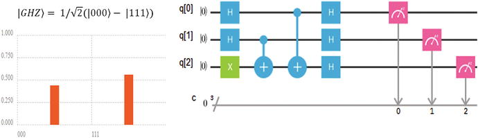
- 1.
In the basis circuit, Hadamard gates in qubits 1 and 2 put them in superposition |00,01,01,11>. At the same time, the X gate negates qubit 3; thus we end up with the states
 .
. - 2.
The two CNOT gates entangle all qubits into the state
 .
. - 3.
Finally the three Hadamard gates map step 2 to the state ½(| 000⟩ − | 111⟩).
Quantum Circuits for GHZ States
Measurement | Results for 100 shots | ||||||||||
|---|---|---|---|---|---|---|---|---|---|---|---|
YYX
|
| ||||||||||
YXY
|
| ||||||||||
XYY
|
| ||||||||||
XXX
|
|
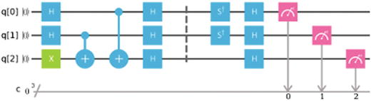
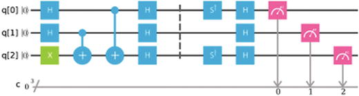
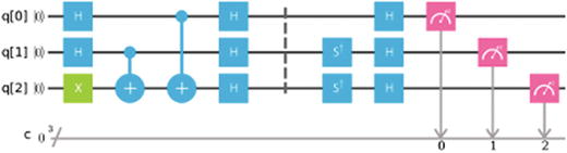
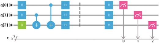
For the measurement of X, apply the H gate to the corresponding qubit.
For each instance of Y, apply the S† (S-dagger), and H gates to the corresponding qubit.
Finally compare the results of the preceding experiment against the official data from IBM Q Experience.3 How do your results stack up? All in all, the principles of quantum mechanics shown in this section have been challenged by a theory called super determinism which gives a way out.
Super Determinism: A Way Out of the Spookiness. Was Einstein Right All Along?
In an interview for BBC in 1969, physicist John Bell talked about his work on quantum mechanics. He said that we must accept the predictions that actions are transferred faster than the speed of light between entangled particles but at the same time we cannot do anything with it. Information cannot travel faster than the speed of light, a fact that is also predicted by quantum mechanics. As if nature is playing a trick on us. He also mentioned that there is a way out of this riddle through a principle called super determinism.
Particle entanglement implies that measurements performed in one particle affect the other instantaneously, even across large distances (think opposite sides of the galaxy or the universe), even across time. Einstein was an ardent opponent of this theory famously writing to Niels Bohr God does not throw dice. He could not accept the probabilistic nature of quantum mechanics, so in 1935, along with colleagues Podolsky and Rosen, they came up with the infamous EPR paradox to challenge its foundation. In the EPR paradox, if two entangled particles are separated by a tremendous distance, a measurement in one could not affect the other instantaneously as the event will have to travel faster than the speed of light (the ultimate speed limit in the universe). This will violate general relativity, thus creating a paradox: Nothing travels faster than the speed of light, that is, the absolute rule of relativity.
Nevertheless, in 1982 the predictions of quantum mechanics were confirmed by French physicist Alain Aspect. He devised an experiment that showed Bell’s inequality is violated by entangled photons. He also proved that a measurement in one of the entangled photons travels faster than the speed of light to signal its state to the other. Since then, Aspect’s results have been proven correct time and again (details on his experiment is shown in Chapter 1). The irony is that there is a chance that Einstein was right all along and entanglement is just an illusion. It is the principle of super determinism.
Tip
In simple terms super determinism says that freedom of choice has been removed since the beginning of the universe. All particle correlations and entanglements were established at the moment of the Big Bang. Thus there is no need for a faster-than-light signal to tell particle B what the outcome of particle A is.
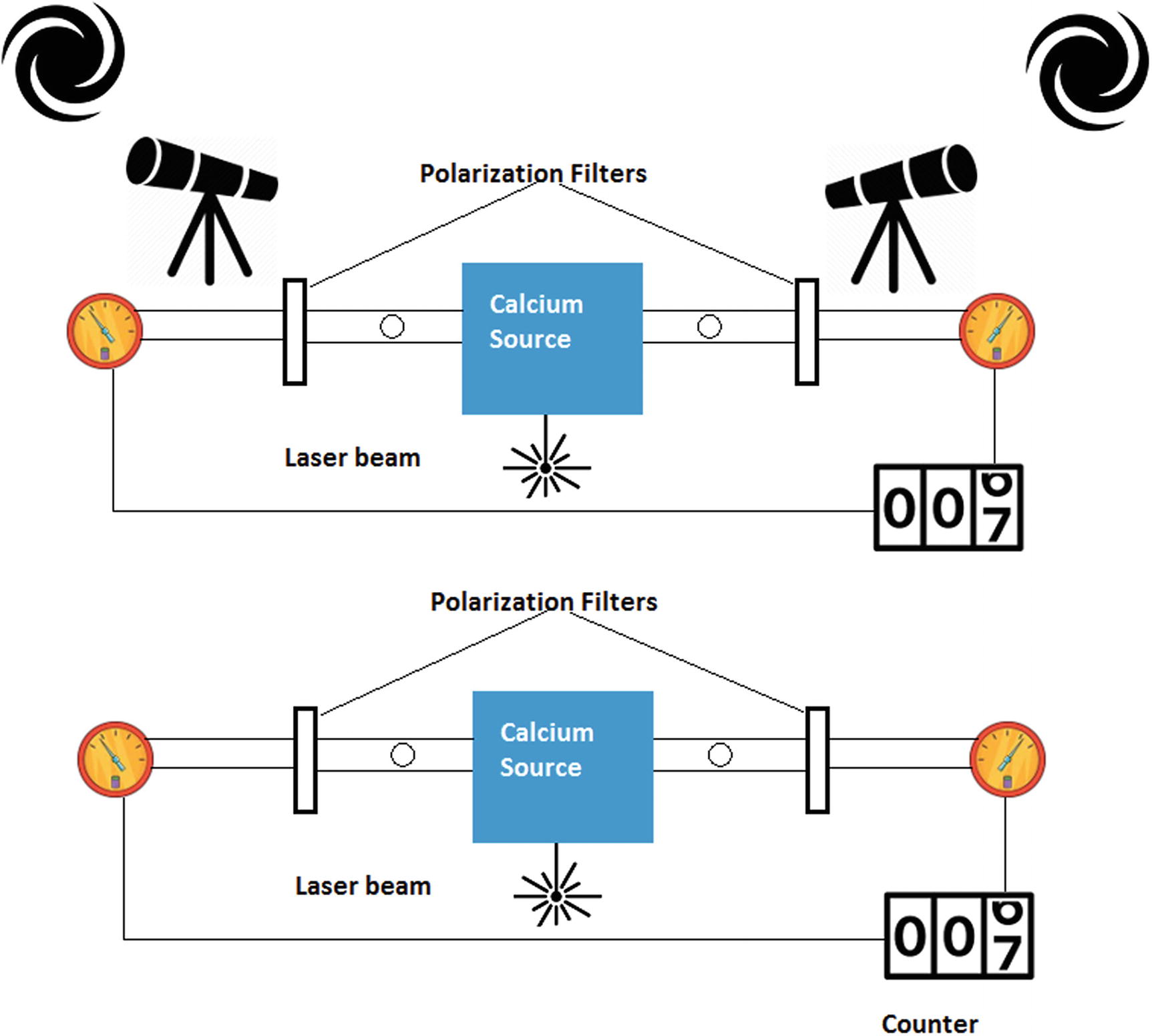
Bell’s inequality experiment using cosmic photons vs. the standard test
Figure 3-5 shows the standard Bell’s inequality test experiment (at the bottom) and a variation of the experiment using cosmic photons (at the top) by Andrew Friedman and colleagues at MIT.4
Tip
For a full description of the standard Bell’s inequality test, see Chapter 1, EPR Paradox Defeated: Bohr Has the Last Laugh.
Friedman and colleagues came up with a novel variation of the standard Bell experiment using cosmic rays. The idea is to use real-time astronomical observations of distant stars in our own galaxy, distant quasars, or patches of the cosmic microwave background, to essentially let the universe decide how to set up the experiment instead of using a standard quantum random number generator. That is, photons from the distant galaxies are used to control the orientation of the polarization filters just prior to the arrival of entangled photons.
If successful, the implications would be groundbreaking. If the results from such experiment do not violate Bell’s inequality, it would mean that super determinism could be true after all. Particle entanglement will be an illusion, and signal transfer between entangled particles could not travel faster than light as predicted by relativity. Einstein will be right and there is no spooky action at a distance.
Luckily for us, fans of quantum mechanics, no such thing has happened so far. Keep in mind that Friedman and colleagues are not the only team getting it on the action. There are multiple teams trying to crack this riddle. As a matter of fact, most of their results agree with quantum mechanics. That is, their results violate Bell’s inequality. So it seems that the rift created by Einstein and Bohr in their struggle between relativity and quantum mechanics long ago is alive and well. My money is in quantum mechanics though. Moving on, the next section shows how IBM Q Experience can be accessed remotely via its slick REST API.
Remote Access via the REST API
QISKit : The Quantum Information Software Kit is the de facto access tool for quantum programming in Python.
IBMQExperience : A lesser known library bundled with QISKit that wraps the REST API in a Python client.
In this section we peek inside IBMQExperience and look at the different REST end points for remote access. But first, authentication is required.
Authentication
Using your API token: To obtain the API token, log in to the IBM Q Experience console and follow the instructions in the following section.
Using your account username and password: Let’s see how this is done using REST.
Tip
To obtain your API token, log in to the IBM Q Experience console, click your username ➤ My Account, and then click the Advanced tab on the upper right. Finally click Generate and then Copy API Token (see Figure 3-6). Always keep your token secure.
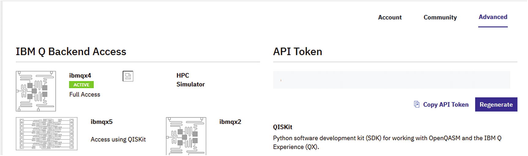
Obtain your API token from the console
Authentication via API Token
HTTP Method: POST
URL: https://quantumexperience.ng.bluemix.net/api/users/loginWithToken
Payload: {“apiToken”: “YOUR_API_TOKEN”}
Authentication via User-Password
HTTP Method: POST
URL: https://quantumexperience.ng.bluemix.net/api/users/login
Payload: {“email”: “USER-NAME”, “password”: “YOUR-PASSWORD”}
Where id is your access token, ttl is the time to live (or expiration time) in milliseconds, and userId is your user id. Save the access token and the user id for use in this section. Note that when your session expires, a new access token needs to be generated.
List Available Backends
HTTP Method: GET
URL: https://quantumexperience.ng.bluemix.net/api/Backends?access_token=ACESS-TOKEN
Request Parameters
Name | Value |
|---|---|
access_token | Your account access token |
HTTP Headers
Name | Value |
|---|---|
x-qx-client-application | Defaults to qiskit-api-py |
Response Sample
Available Backend Response Keys
Key | Description |
|---|---|
Name | The name id of the processor to be used when executing code against it. |
Version | A string or positive integer probably used to track changes to the processor. |
Description | This is probably a description of the hardware used to build the chip. You may see things like: • 5 transmon bowtie • 16 transmon 2x8 ladder Note: a transmon is defined as a type of noise-resistant superconducting charge qubit. It was developed by Robert J. Schoelkopf, Michel Devoret, Steven M. Girvin, and their colleagues at Yale University in 2007.5 |
basisGates | These are the physical qubit gates of the processor. They are the foundation under which more complex logical gates can be constructed. |
nQubits | The number of qubits used by the processor. |
couplingMap | The coupling map defines interactions between individual qubits while retaining quantum coherence. It is used to simplify quantum circuitry and allow the system to be broken up into smaller units. |
Get Calibration Information for a Given Processor
Request Parameters
Name | Value |
|---|---|
access_token | Your account access token. |
HTTP Headers
Name | Value |
|---|---|
x-qx-client-application | Defaults to qiskit-api-py (a default value for the official client although I suspect it can be anything). |
Response Sample
gateError: This is the error rate of a qubit gate operation at a given time.
readoutError: This is the error rate of a qubit readout operation at a given time.
Tip
Qubit quality evaluation involves four stages (operations): preparation, memory, gates, and readout. Error rates are calculated at the gate and readout stages to track the quality of the qubit. This is the information returned by this API call. Note that after usage qubits must be reset (cooled down) to a basis state.
Simplified Response for the Calibration Parameters If ibmqx4
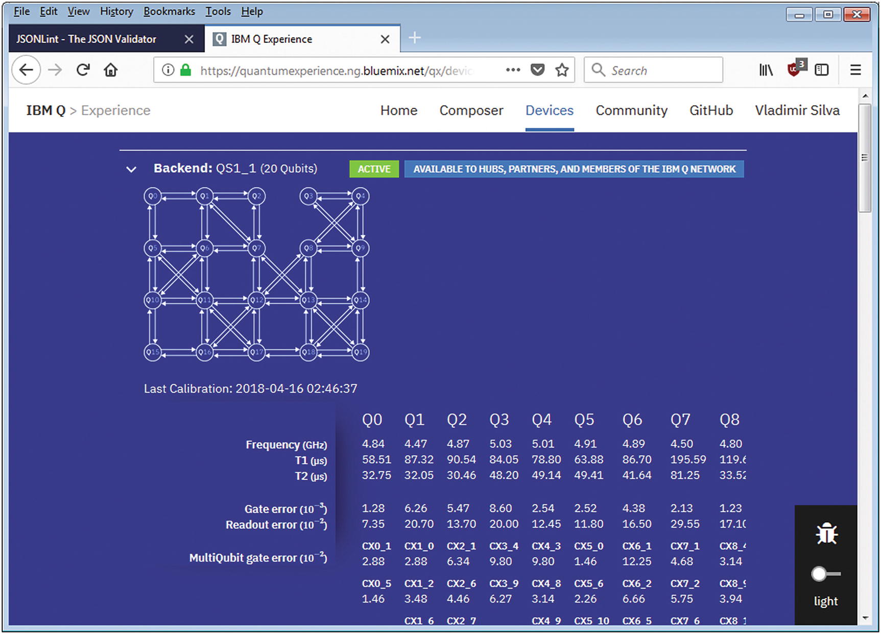
Calibration information reported by the web console
Get Backend Parameters
Qubit cooldown temperature in Kelvin degrees: For example, I got 0.021 K for ibmqx4 – that is, a super frosty –459.6 °F or –273.1 °C.
Buffer times in ns.
Gate times in ns.
Other quantum specs documented in more detail at the backend information site.7
Request Parameters
Name | Value |
|---|---|
access_token | Your account access token |
HTTP Headers
Name | Value |
|---|---|
x-qx-client-application | Defaults to qiskit-api-py |
Response Sample
Simplified Response for ibmqx4 Parameters
Get the Status of a Processor’s Queue
HTTP Method: GET
URL: https://quantumexperience.ng.bluemix.net/api/Backends/NAME/queue/status
Request Parameters
It seems strange but this API call appears not to ask for an access token.
HTTP Headers
Name | Value |
|---|---|
x-qx-client-application | Defaults to qiskit-api-py |
Response Sample
For example, to get the event queue for ibmqx4, paste the following URL in your browser:
https://quantumexperience.ng.bluemix.net/api/Backends/ibmqx4/queue/status
state: It is the status of the processor. If alive, true else false.
status: It is the status of the execution queue – active or busy.
lengthQueue: It is the size of the execution queue or the number of simulations waiting to be executed.
Tip
When you submit an experiment to IBM Q Experience, it will enter an execution queue. This API call is useful to monitor how busy the processor is at a given time.
List Jobs in the Execution Queue
Request Parameters
Name | Value |
|---|---|
access_token | Your account access token. |
filter | A result size hint in JSON. For example, {“limit”:2} returns a maximum of two entries. |
HTTP Headers
Name | Value |
|---|---|
x-qx-client-application | Defaults to qiskit-api-py |
Response Sample
Simplified Response for the Get Jobs API Call
Note
Depending on the size of the execution queue, you may get an empty result ([ ]) if there are no jobs in queue or a formal result as shown in Listing 3-4. Whatever the case make sure the HTTP response code is 200 (OK).
Get Account Credit Information
HTTP Method: GET
URL: https://quantumexperience.ng.bluemix.net/api/users/USER-ID?access_token=ACCESS-TOKEN
Tip
The user id can be obtained from the authentication response via API token or user-password. See the “Authentication” section for details.
Request Parameters
Name | Value |
|---|---|
access_token | Your account access token. |
HTTP Headers
Name | Value |
|---|---|
x-qx-client-application | Defaults to qiskit-api-py |
Response Sample
Credit Information Sample Response
List User’s Experiments
Request Parameters
Name | Value |
|---|---|
USER-ID | Your user id obtained from the authentication step. |
access_token | Your account access token. |
includeExecutions | If true, include executions in the result. |
HTTP Headers
Name | Value |
|---|---|
x-qx-client-application | Defaults to qiskit-api-py |
Response Sample
Experiment List Response
Run Experiment
Request Parameters
Name | Value |
|---|---|
shots | The number of shots to perform. The higher the number, the better the accuracy of your results will be. Note that this number depletes your credits at a rate of 3 credits per 1024 shots. Space is at a premium in the quantum world. |
access_token | Your account access token. |
deviceRunType | The device where to run the experiment. This could be • A real device name such as ibmqx2 and ibmqx3 for real processors. • For simulators: simulator or sim_trivial_2. |
seed (optional) | An optional random number required only for simulators. |
HTTP Headers
Name | Value |
|---|---|
x-qx-client-application | Defaults to qiskit-api-py |
Content-Type | application/json |
Payload Format
Response Sample
Bell State XW Measurement
Now we are ready to submit our experiment via REST. Don’t forget that you must authenticate first to obtain an access token.
Tip
REST clients are available for most if not all current browsers. Install your favorite browser REST client, and create an authentication request as described in the “Authentication” section. Save it and keep it handy to obtain your access token.
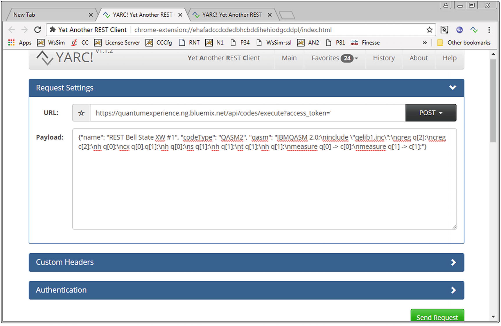
Chrome’s YARC REST client with payload for Bell state XW experiment
Submit to the Simulator
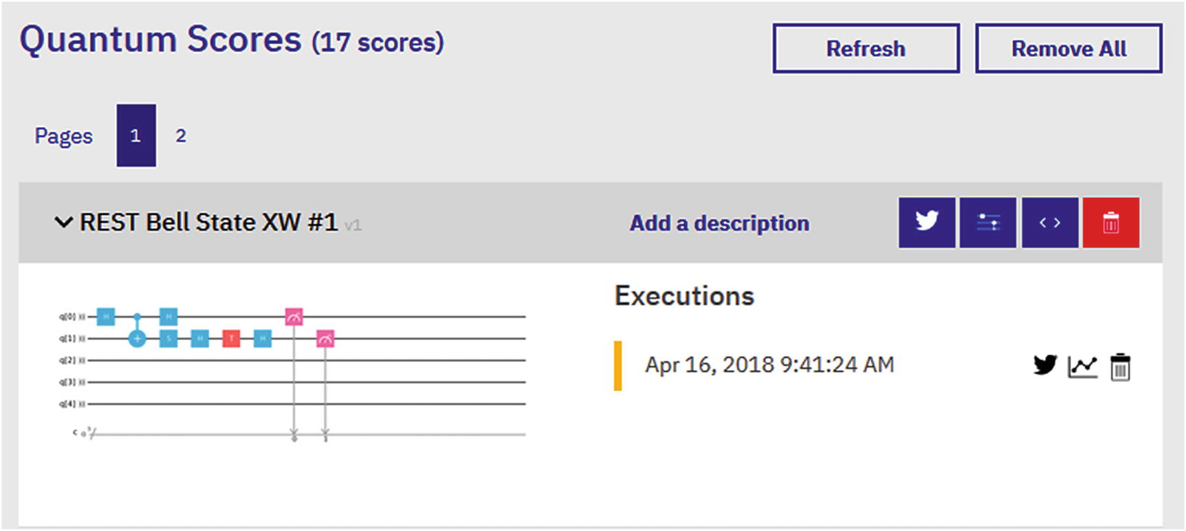
Web console showing the Bell state XW experiment submitted via REST
Submit to a Real Device
Note
Real quantum devices may be offline for maintenance or whatever reason. If that is the case, the submission will fail with a 400 (bad request) HTTP response. Make sure the device is online before submitting to a real quantum device!
Simplified HTTP Response from the Bell State XW Experiment Submitted via REST
At this point, you have succeeded submitting your first experiment via REST. Try playing by increasing the number of shots of your experiment to achieve greater accuracy.
Run a Job
End point 1: For regular users of the IBM Q Experience.
End point 2: For corporate customers. It requires a hub, group, and project ids.
HTTP Method: POST
URL 1: (5, 16 qubits) https://quantumexperience.ng.bluemix.net/api/Jobs?access_token=ACCESS-TOKEN
URL 2: (20+ qubits corporate) https://quantumexperience.ng.bluemix.net/api/Network/HUB/Groups/GROUP/Projects/PROJECT/jobs?access_token=ACCESS-TOKEN
Request Parameters
Name | Value |
|---|---|
access_token | Your account access token |
HTTP Headers
Name | Value |
|---|---|
x-qx-client-application | Defaults to qiskit-api-py |
Content-Type | application/json |
Payload Format
Tip
Experiments submitted through the Run Job end point are not recorded in the Scores section of the Composer but put in an execution queue for processing.
On the other hand, a submission via the Run Experiment end point will record an entry in the Composer. Also, note that any experiment submitted to the simulator will return results immediately. Experiments submitted to a real quantum device will always enter the execution queue in a PENDING state. On completion, a notification email will be sent to the user. Let’s send a quick job to the real device ibmqx4. Paste the following end point into your REST client:
https://quantumexperience.ng.bluemix.net/api/Jobs?access_token=access_token
Note that my job won’t show up in the Composer; however I will get an email with a link to the results.
Get the API Version
HTTP Method: GET
URL: https://quantumexperience.ng.bluemix.net/api/version?access_token=ACCESS-TOKEN
Request Parameters
Name | Value |
|---|---|
access_token | Your account access token |
HTTP Headers
Name | Value |
|---|---|
x-qx-client-application | Defaults to qiskit-api-py |
Response Format
It returns a string with the version of the API, by the time of this writing 6.4.8.
We have peaked inside the Python IBMQuantumExperience REST API to see what goes on behind the scenes. As an exercise let’s build a custom client for Node JS. Here is how.
A Node JS Client for the IBMQuantumExperience
IBMQuantumExperience : This is a REST client implementation in Python which I peeked into to present the REST API from the previous section. This library is not well documented. It makes sense as it is meant to be a modularized library that may change in the future.
QISKit SDK : This is the main entry point to all your quantum programs. It packs gate logic; assembly translation; simulators, a local python simulator and a fast C++ simulator; and much more. This library also invokes IBMQuantumExperience for all interactions via REST to the IBM Q Experience platform.
Node JS is a powerhouse for network I/O asynchronous calls. It is fast, and it is the perfect platform for REST clients.
Python is a good language, with a plethora of amazing numerical, math, chart libraries, but has some idiosyncrasies that some may find unattractive. For example, indentation is relevant in Python (you cannot mix TABS and spaces – there are no braces to differentiate blocks). This drove me crazy at the beginning and took me a while to figure out as almost all computer languages use braces to differentiate logic blocks. No such thing in Python, you must use spaces or TABS and you cannot mix them. I don’t like this. I think it is bad design because if you make a mistake, you don’t know where a logic block ends. That’s what braces are for.
Variety is always good: after all my troubles with Python, I thought this library could be the foundation for a QISKit clone for Node JS.
So let’s get started.
Build a Node Module for IBMQuantumExperience
Tip
Linux users: I have used Windows to write this section; furthermore I assume that you have installed Node JS, are familiar with Node modules, and can code in Javascript. All in all, you can get Node installers for all platforms at https://nodejs.org/en/ . Also note that Linux complains about uppercase names for package names. Save yourself a headache and use Windows to go thru this section.
index.js: This is your module code. Note for Linux users, this file may not be created. If so create it manually.
Package.json: This is the module descriptor with information such as name, version, author, dependencies, and more.
The second command installs the popular HTTP request package and all its dependencies in the current folder. Now we are ready to start implementing the REST API from the previous section. Open index.js in your favorite editor and let’s get started.
Export API Methods
Expose Public API Methods via Node
Line 2 imports the request HTTP client library to interact with Q Experience.
- Line 5 declares the public methods to be exposed by this module:
init: This method authenticates against the Q Experience platform as described in the previous section “Remote Access via the REST API.”
getCalibration: It returns the platform’s calibration parameters for a given device.
getBackends: It returns a list of quantum devices (and simulators) available for use.
getParameters: It returns the device parameters as described under the Devices section of the Composer web console.
runExperiment: It runs an experiment remotely in the simulator or real quantum device.
getJobs: It returns a list of current jobs in the experiment execution queue.
getMyCredits: It returns the user’s execution credit and other useful information.
Authenticate with a Token
Token Authentication via REST
The request.post system call is used to send an HTTP POST to the end point https://quantumexperience.ng.bluemix.net/api/users/loginWithToken using the JSON payload {'apiToken': 'YOUR_TOKEN'}. As described by the REST API, this call returns a new JSON document: {"id":"TOKEN","ttl":1209600,"created":"DATE","userId":"USERID"}. This document is parsed and the access token (id) and user id (userId) saved for later use.
Note that because all network I/O in Node is asynchronous, all methods return a Promise. This is basically an asynchronous task that encapsulates the difficulty of having to wait for the task to complete before reading results. Thus if the HTTP request call succeeds, the resolve callback from the Promise will fire with the HTTP response data; else the Promise reject callback will be invoked.
Tip
Promises are a compelling alternative to callbacks for asynchronous code. Nevertheless they can be confusing some times. All in all, Promises are becoming the de facto standard for asynchronous programming in Javascript.
Nevertheless if you find the Promise handling code convoluted, there is an even easier way to deal with this, and it is shown in the next section where we implement a method to fetch the list of backends.
List Backends
It sends an HTTP GET request to https://quantumexperience.ng.bluemix.net/api/Backends?access_token=TOKEN .
It returns a Promise which can be called within any asynchronous function by using the new async/await feature in Javascript.
Get Backend List via Node
Tip
An async function can contain an await expression that pauses the execution of the async function and waits for the passed Promise’s resolution and then resumes the async function’s execution and returns the resolved value.
List Calibration Parameters
Fetch calibration information by sending a GET request to https://quantumexperience.ng.bluemix.net/api/Backends/NAME/calibration?access_token=TOKEN where NAME is the backend you wish to query and TOKEN is the access token obtained from the authentication step.
Fetch backend parameters by sending a similar GET request to https://quantumexperience.ng.bluemix.net/api/Backends/NAME/parameters?access_token=TOKEN .
The response format for both requests is described in the Remote Access via the REST API section of this chapter.
Get Device Calibration and Parameter Data
For the final step, let’s see how an experiment can be run.
Run the Experiment
Remember that the assembly code must be formatted in a single line with line feeds (\n) to separate instructions. For example, the following code declares 5 qubits and 5 classical registers: "\n\ninclude \"qelib1.inc\";\nqreg q[5];\ncreg c[5];\n".
The name parameter defines the experiment name to be recorded in the web console.
The shots parameter is the number of shots executed by the quantum processor.
The device parameter can be simulator (for the remote simulator) or a real quantum device name such as ibmqx4.
Tip
If you run an experiment in a real device, it will enter an execution queue for future processing. You will receive an email on completion. On the other hand, if you run the experiment in the remote simulator, the results will be returned synchronously.
Run an Experiment
Tip
The code for the IBMQuantumExperience Node module is included in the book source under Workspace\Ch03\IBMQuantumExperience. The project has a test script under test/tests.js. Edit this file, add your API token, and execute it from IBMQuantumExperience with the command: node test/tests.js.
Debugging and Testing
To run the test, execute node test\tests.js within the IBMQuantumExperience folder. Note that I have left out two methods: getJobs and getMycredits as an exercise. With this foundation, you should be able to easily implement and test them.
Share with the World: Publish Your Module
In this chapter you have taken the first step in your new career as a quantum programmer. IBM has created an amazing cloud platform to learn about these incredible machines. We should thank the good folks at IBM for making this platform freely accessible to the masses. For now, quantum computers are experimental machines, so don’t expect to get one at the local hardware store. Nevertheless soon they will take over the data center, so now is the time to learn how to program them.