Vladimir SilvaPractical Quantum Computing for Developershttps://doi.org/10.1007/978-1-4842-4218-6_2

2. Quantum Computing: Bending the Fabric of Reality Itself

Vladimir Silva¹

(1)

CARY, NC, USA

Semiconductors have come a long way since the days of the vacuum tube. It is hard to believe that the transistor today is around 14 nanometers in size (i.e., close to a molecule). In this chapter you will learn about the origins of quantum computing starting with the fate of the transistor. It seems that the semiconductor process and the transistor are in a collision course with the laws of physics. Next, an in-depth look at the basic component of a quantum computer: the qubit including the strange effects of superposition, entanglement, and qubit manipulation using logic gates. Furthermore, qubit design is an important topic, and this chapter describes the leading prototypes by major IT companies including pros and cons of each.

You will also learn about how quantum computers stack against traditional ones at this point. Things are a little rough for quantum right now, but that is about to change in the next few years. Still, quantum computers face a few pitfalls inherit to the theory of quantum mechanics: they are fragile and error prone; find out why. This chapter also discusses the very interesting quest toward the so-called quantum supremacy. The battle is fierce between IT giants with no winner in sight. Another topic of discussion is the controversial field of quantum annealing and the difference with the standard quantum gate approach used all over this book.

The chapter ends with the path toward universal quantum computation including efforts by all major vendors: in the short term, expect to see quantum computers in the data center. In the long term, the future looks bright with significant resources being poured into fields such as aerospace, medicine, artificial intelligence, and others. The race is getting global. Let’s get started.

The Transistor Is in a Collision Course with the Laws of Physics

Out of curiosity, have you ever looked inside your home PC to see what it is made of? It is basically a silicon motherboard full of all kinds of electronic gizmos, and in the center rests the big black square that is the CPU. Depending on what kind of PC you have, there may be multiple CPUs, graphics processing units (GPUs), audio, network cards, and all sorts of modularized components. All these components are made of millions of transistors, the fundamental building block of many electronics. A transistor is essentially tiny switch with an on/off position allowing electrons to either pass or not. This property is in turn used to encode a 0 or 1, the basis of the binary language used by all electronics.

Transistors are combined to create logic gates (see Table 2-1). These gates, in turn, produce the fundamental arithmetic functions: addition, subtraction, multiplication, and division. These simple operations provide all the power we need to run powerful scientific simulations, play games, encrypt data, browse the Web, email friends, you name it.

Table 2-1

Basic Logic Gates

Type

Symbol

Description

Truth table

NOT

../images/469026_1_En_2_Chapter/469026_1_En_2_Figa_HTML.jpg

Negates the input.

A	~A
0	1
1	0

AND

../images/469026_1_En_2_Chapter/469026_1_En_2_Figb_HTML.jpg

Logical product.

A	B	A AND B
0	0	0
0	1	0
1	0	0
1	1	1

../images/469026_1_En_2_Chapter/469026_1_En_2_Figc_HTML.jpg

Logical addition.

A	B	A OR B
0	0	0
0	1	1
1	0	1
1	1	1

NAND

../images/469026_1_En_2_Chapter/469026_1_En_2_Figd_HTML.jpg

Negates the logical product.

A	B	A NAND B
0	0	1
0	1	1
1	0	1
1	1	0

NOR

../images/469026_1_En_2_Chapter/469026_1_En_2_Fige_HTML.jpg

Negates the logical addition.

A	B	A NOR B
0	0	1
0	1	0
1	0	0
1	1	0

XOR

../images/469026_1_En_2_Chapter/469026_1_En_2_Figf_HTML.jpg

Exclusive OR: The output of a two-input XOR is 1 only, when the two input values are different, and 0 if they are equal.

A	B	A XOR B
0	0	0
0	1	1
1	0	1
1	1	0

Transistors have given our society tremendous technological advances. They are everywhere: computers, communication devices, medicine equipment, aerospace hardware, and others. Whatever machine you can think of is probably made of transistors, yet the transistor is about to face an impassable barrier: the laws of physics, specifically quantum mechanics.

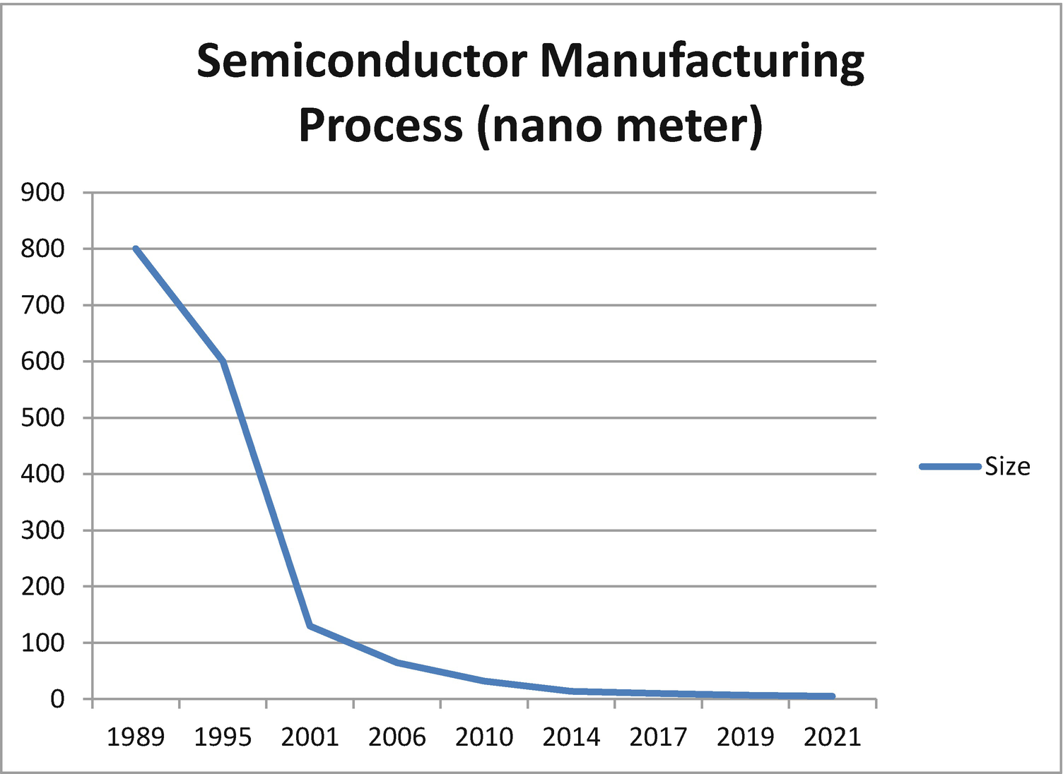
Five-Nanometer Transistor : Big Problem

Since the 1960s traditional computers have grown exponentially in power, at the same time becoming smaller and smaller. Today, computers are made of millions of transistors, but once a transistor starts to get close to the size of an atom, the bizarre world of quantum mechanics kicks in and all bets are off.

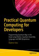
Consider Figures 2-1 and 2-2, showing the semiconductor manufacturing process sizes from 1970 to 2020. From a size of around 10 micrometers in the 1970s, sizes become smaller and smaller (at around 1 micrometer) by the late 1980s. Even scarier, there is a huge dip into the nanometer scale (1 nanometer = 10^-9 m) from the 1990s until the present and beyond (see Figure 2-2). We are talking about transistors approaching the size of molecules. By 2020 the size of a transistor will be around 5 nanometers . At this scale, the bizarre properties of quantum mechanics may start to wreak havoc in the classical computer.

../images/469026_1_En_2_Chapter/469026_1_En_2_Fig1_HTML.png — Figure 2-1
Semiconductor sizes from the 1970s through the 1980s

Table 2-2

Semiconductor Size Data for Figure 2-1

Year	Size in micrometers
1971	10
1974	6
1977	3
1982	1.5
1985	1

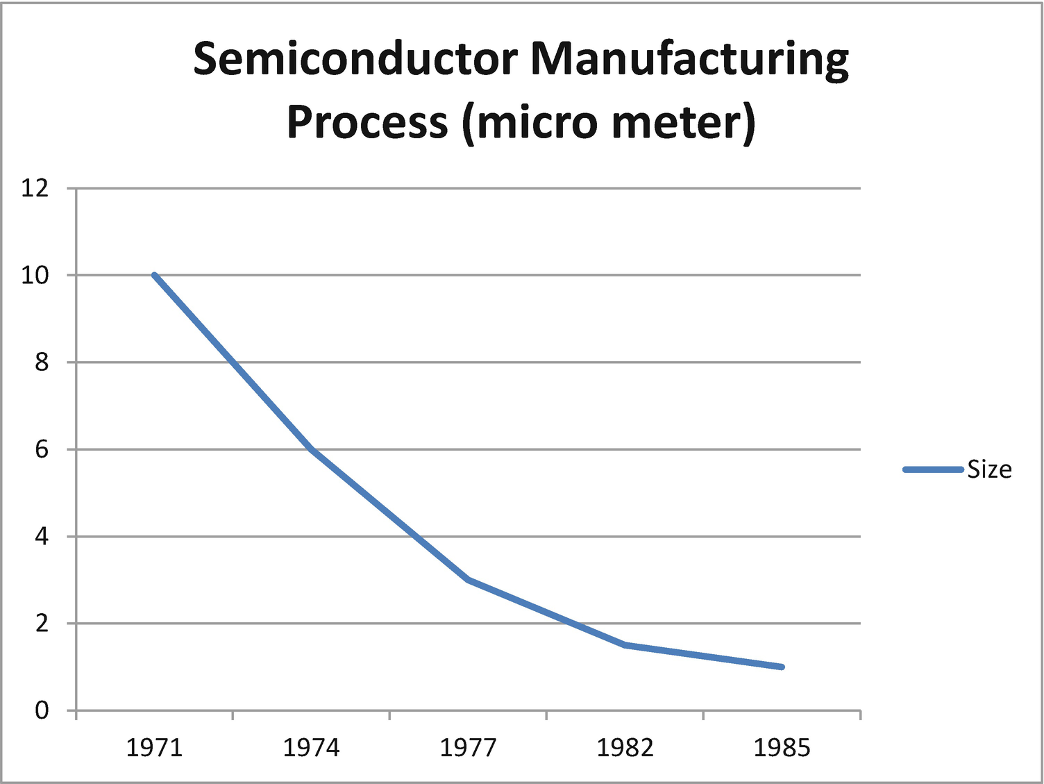
../images/469026_1_En_2_Chapter/469026_1_En_2_Fig2_HTML.png — Figure 2-2
Semiconductor sizes from the 1990s and beyond

Table 2-3

Semiconductor Size Data for Figure 2-2

Year	Size in nanometers
1995	600
2001	130
2010	32
2014	14
2019	7
2021	5

Figure 2-3 shows the size of a transistor by 2020 (around 5 nm) vs. a water molecule (0.275 nm). Unfortunately sizes can’t keep getting smaller forever. There is a threshold that will render classical computers useless, and it is called the quantum scale.

../images/469026_1_En_2_Chapter/469026_1_En_2_Fig3_HTML.jpg — Figure 2-3
Transistor size against a water molecule

Quantum Scale and the Demise of the Transistor

Perhaps the demise of the transistor will be an exaggeration. Nevertheless, what is not is the term quantum scale and its effects on it. In physics, quantum scale is the distance where quantum mechanical effects become apparent in an isolated system. This strange boundary lives at scales of 100 nm or less or at a very low temperature. Formally, the quantum scale is the distance at which the action or angular momentum is quantized.

Quantum effects can cascade into the microscale realm causing problems for current microelectronics. The most typical effects are electron tunnelling and interference as shown by the single-double slit experiment.

Electron Tunnelling

Electron tunnelling, also known as quantum tunnelling, is the phenomenon where a particle passes through a barrier that otherwise could not be surmounted at a classic scale. This spells trouble for the transistor and here is why.

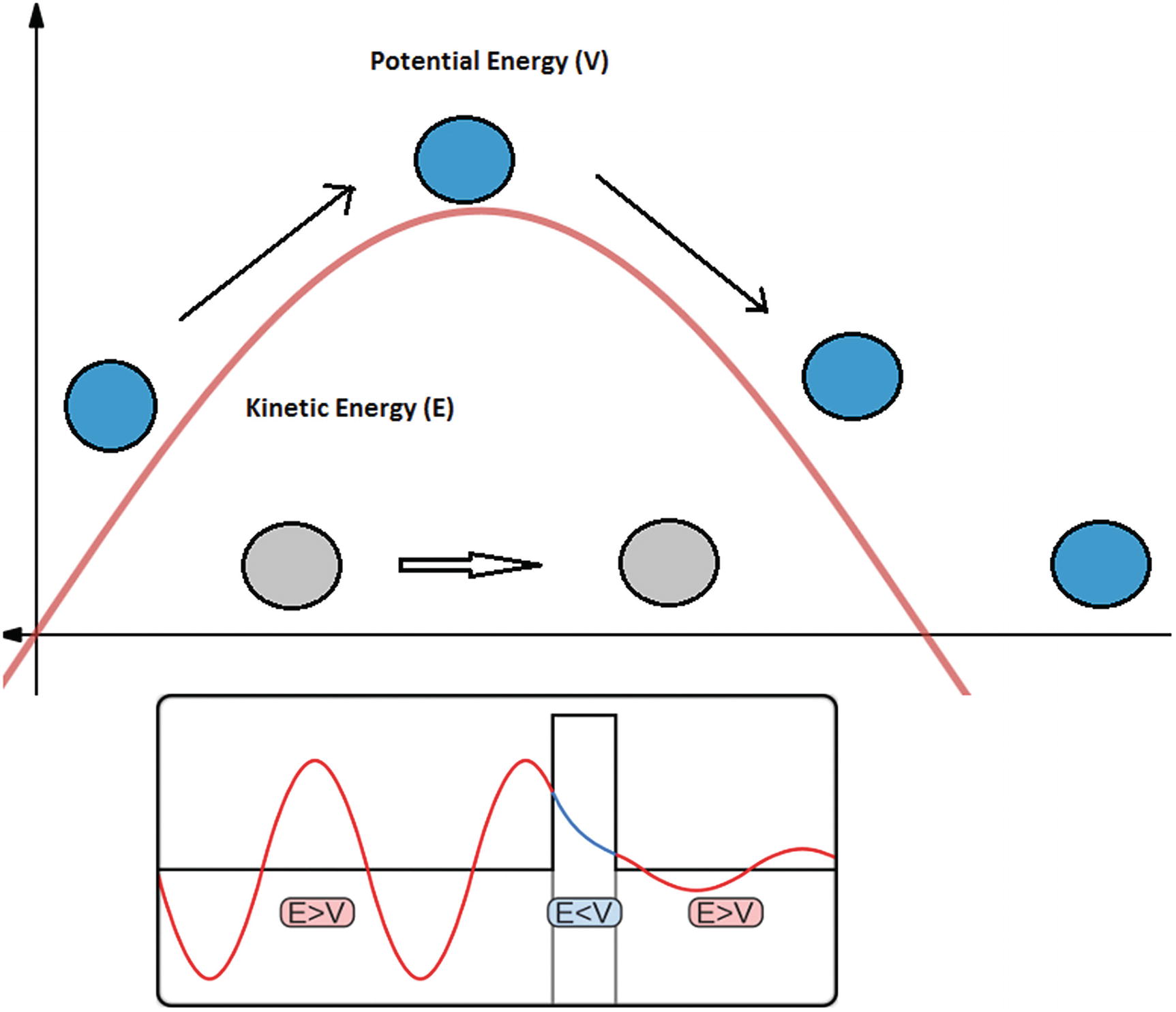
Assume that we have a particle with energy E trying to surmount a barrier with potential energy V at the top. According to the classical law of the conservation of energy, the particle needs its energy E > V to pass through, that is, the kinetic energy of the particle must be greater than the potential energy V (see Figure 2-4).

../images/469026_1_En_2_Chapter/469026_1_En_2_Fig4_HTML.jpg — Figure 2-4
Quantum tunnelling in action

Note

Electron tunnelling may spell doom for the transistor, yet one’s loss is someone else’s gain. This important property led to the development of the scanning tunnelling microscope (STM) which had a profound impact on chemical, biological, and materials science research.

Figure 4 shows the effects of classical mechanics as well as quantum tunnelling. According to quantum mechanics, there is a probability that the electron will pass through the barrier even if its kinetic energy is less than the potential energy of the barrier (E < V). This is due to Heisenberg uncertainty principle (HUP). In the previous chapter, you learned about the duality behavior of photons and other particles: both as waves and particles. For waves, Schrödinger’s wave function rules, for particles, Niels Bohr described changes in the state of an atom when it gains or losses energy (quantum jumps). The uncertainty principle bridges the gap by introducing the probability of the position and momentum of a particle at a given time.

When a particle such as an electron or photon approaches a barrier (such as a transistor), there is a probability it will go straight through it. This is because its wave function diminishes from sinusoidal to an exponential form,¹ and its solution becomes Equation 2.1.

$\varPsi =N{e}^{-\beta x}$

(2.1)

$P=\exp \left(-\frac{4 a\varPi}{\mathrm{h}}\sqrt{2m\kern0.28em \left(V-E\right)}\right)$

(2.2)

where

ψ is Schrödinger’s diminished wave function.
N is a normalization constant.
$\beta =\sqrt{2m\kern0.28em \left(V-E\right)/{h}^2}$
m is the mass of the particle.
V is the potential energy and E is the kinetic energy.
h is the Planck constant 6.626x10⁻³⁴ m²kg/s.
a is the thickness of the barrier.

According to Engel¹, the probability P that the particle will pass through the barrier can be calculated by formula 2.2. Furthermore for quantum tunnelling to occur, the following conditions must be met:

The height of the barrier must be finite and the thickness of the barrier should be thin.
The potential energy of the barrier exceeds its kinetic energy (E<V).
The particle has wave properties suggesting that quantum tunnelling only applies to nanoscale objects such as electrons, photons, etc.

Let’s have some fun by calculating quantum tunnelling probabilities for various barrier sizes of the current semiconductor manufacturing process. The next sections present a series of exercises to visualize this process in detail.

Exercise 1

Calculate the quantum tunnelling probability for the electron using your favorite tool (e.g., an Excel spreadsheet) for formula 2.2 assuming the following values:

Kinetic energy of the electron E = 4.5 eV.
Rectangular barrier with potential energy V = 5 eV. Remember that, for quantum tunnelling to occur, E < V.
Use the size of the barrier provided by the semiconductor manufacturing process in the previous section at the quantum scale; thus size < 100 nm for years 2000 and beyond (use Tables 2-2 and 2-3 from the previous section).
Don’t forget the Planck constant h = 6.626x10⁻³⁴ and the mass of the electron m = 9.1x10⁻³¹ kg.

Tip

eV is the electron volt, the basic unit of energy in quantum mechanics. 1 eV = 1.6X10^-19 joules (J). This value is required for unit conversion in the probability calculation.

Solution 1

I have used an Excel spreadsheet to easily calculate values from a table and formula which is included in the source code of this manuscript. Thus pick a cell in your Excel and type formula 2.2. Remember that the part (V-E) must be reduced by multiplication by 1.6X10⁻¹⁹ J/eV. Thus formula 2.2 in Excel becomes

EXP(((−4*D5*3.14)/(6.626E−34)) * SQRT(2 * (9.1E−31) * (5 − 4.5) * (1.6E−19)))

In the formula above, cell D5 contains the barrier size, and the rest are the constants π = 3.14, h = 6.626e⁻³⁴, m = 9.1e⁻³¹, and 1 eV =1.6x10¹⁹ J. With the formula in place, create a new table with the manufacturing year and barrier sizes in nanometers (from Tables 2-2 and 2-3). Finally, make a logic copy of the formula across the cell data for all years and barrier sizes (see Table 2-4).

Table 2-4

Electron Tunnelling Probabilities for the Semiconductor Process

Year	Barrier size (m)	Probability
1989	0.0000008	0
2001	1.30E−07	0
2006	0.000000065	6.5829E−205
2010	0.000000032	3.0188E−101
2014	0.000000014	1.053E−44
2017	1.00E−08	3.86767E−32
2019	7.00E−09	1.02616E−22
2021	5.00E−09	1.96664E−16
Beyond	5E−10	0.026876484

What conclusions can be drawn from this data?

The probability appears to be low, even for the 5 nm manufacturing process coming up in 2021 (1.9e−16). Remember that this value must be multiplied by 100 to obtain a percentage.
At a barrier size of around 500 picometers (pm), things start to get a little scary. The probability is 0.0268; thus there is 2.68% chance that an electron will pass through the barrier. This means that, for example, if you send some encoded message, 2.68% of the bits will be lost! Not good.

Tip

A picometer (pm) is 1/1000 of a nanometer or 10e⁻¹² meters.

Exercise 2

Write a tiny program, in your favorite programming language, to calculate the probability as shown in the previous exercise. Verify that the results are the same. Dump the results to standard output as shown in the paragraph below.

Quantum tunnelling probabilities for current semiconductor processes.

2001 1.30e-07 0.000e+00

2010 3.20e-08 2.684e-101

2014 1.40e-08 1.000e-44

2019 7.00e-09 1.000e-22

2021 5.00e-09 1.931e-16

Beyond 5.00e-10 2.683e-02

Solution 2

Listing 2-1 shows a small Java program to calculate the probability for the years and sizes of the current manufacturing process as done in the previous exercise.

public class Quantum Tunnelling {

/** Planck's constant */

static final double K_PLANK = 6.626e-34;

/** Mass of the electron (kg) */

static final double K_ELECTRON_MASS = 9.1e-31;

/** Electron volt */

static final double K_EV = 1.6e-19;

/**

* Engel's Quantum Tunnelling Probability

* @param size

* Size of the barrier in meters.

* @param E

* Kinetic energy in electron volts (eV).

* @param V

* Potential energy in eV.

* @return Quantum Tunnelling Probability

static double EngelProbability(double size, double E, double V) {

if (E > V) {

throw new IllegalArgumentException

("Potential energy (V) must be > Kinetic Energy (E)");

}

double delta = V - E;

double p1 = ((-4 * size * Math.PI) / K_PLANK);

double p2 = Math.sqrt(2 * K_ELECTRON_MASS * delta * K_EV);

return Math.exp(p1 * p2);

}

/** A simple test for current semiconductor processes */

public static void main(String[] args) {

try {

// Barrier sizes for current semiconductor processes (m)

final double[] SIZES = { 130e-9, 32e-9, 14e-9, 7e-9, 5e-9, 500e-12 };

// Dates for display purposes

final String[] DATES = { "2001", "2010", "2014", "2019", "2021", "Beyond" };

final double E = 4.5; // Kinetic energy of the electron (eV)

final double V = 5.0; // Potential energy (eV)

// Display them...

for (int i = 0; i < DATES.length; i++) {

double p = EngelProbability(SIZES[i], E, V);

System.out.println(String.format("%s\t%2.2e\t%2.3e", DATES[i], SIZES[i], p));

}

} catch (Exception e) {

e.printStackTrace();

}

Listing 2-1

Java Program to Calculate the Quantum Tunnelling Probability for the Semiconductor Manufacturing Process 2000 and Beyond

Listing 2-1 defines a function, EngelProbability, that takes three arguments: the size of the barrier in meters, the kinetic energy of the particle (E) in eV, and the potential energy (V) in eV. It applies formula 2.1 and returns the probability. The main program then simply loops through an array for the years of the manufacturing process, String[] DATES = { "2001", "2010", "2014", "2019", "2021", "Beyond"}, and corresponding sizes: double[] SIZES = { 130e-9, 32e-9, 14e-9, 7e-9, 5e-9, 500e-12}. The data is formatted as a table to standard output.

Exercise 3

Plot the data obtained in exercise 1 or 2 into a graph to better visualize the situation. Finally, bravely postulate the year of the demise of the transistor for the current semiconductor manufacturing process!

Solution 3

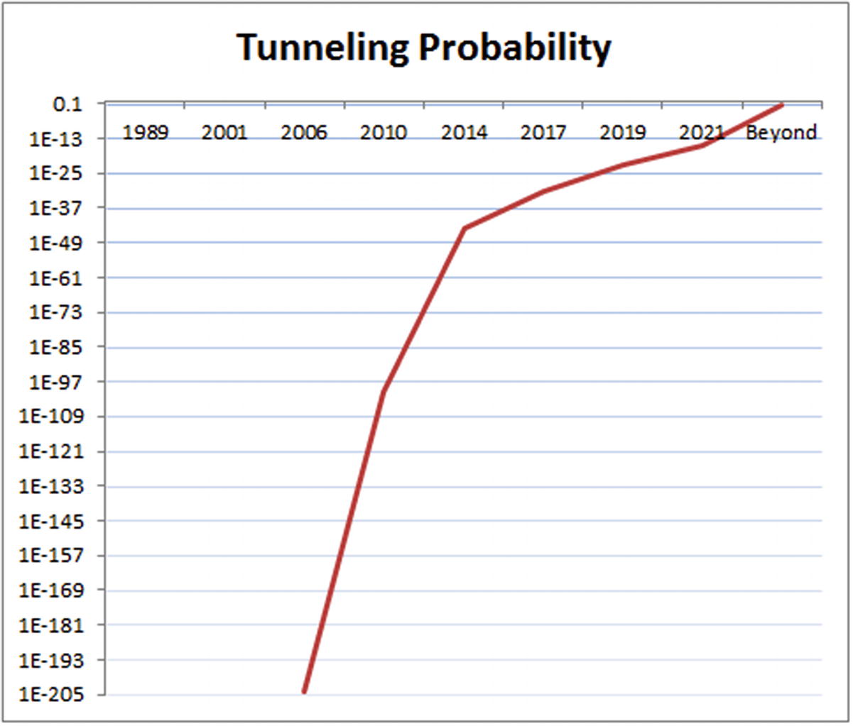
Spreadsheets are such great tools to manipulate statistical values. The previous data can be plotted in a snap into a cool line graph as shown in Figure 2-5.

../images/469026_1_En_2_Chapter/469026_1_En_2_Fig5_HTML.jpg — Figure 2-5
Quantum tunnelling probabilities for the semiconductor manufacturing process

Now for the grand finale, the demise of the transistor should come around year… I feel skeptical about estimating such year. Something I have learned about quantum mechanics is that everything is ruled by uncertainty. If we assume that a 1% probability for quantum tunnelling is unacceptable for the current manufacturing process, then the data above shows that around 2025, at a barrier size between 1 nanometer and 500 picometers, transistors and therefore all computers may become unusable, although my guess is that transistors will evolve into something else, perhaps something organic or weirder. Nevertheless, it is time to start learning to program a quantum computer just in case.

Now let’s look at the next quantum effect causing trouble for the transistor: the uncertainty of the position or momentum shown by basic slit experiments.

Slit Experiments

These experiments were performed many decades ago and are designed as a basic demonstration of the bizarre world of quantum mechanics. They come in many flavors: single slit, double slit, and others. In the single slit experiment, a laser passes through a vertical slit a few inches in width, and it is projected into a surface. The width of the slit can be decreased as desired. As expected we see a dot projected in the surface. Now, if the width of the slit is decreased, the projected dot becomes narrower and narrower; again this is the expected result. But wait, when the width of the slit decreases at about 1/100 of an inch, things get crazy. The dot doesn’t become narrower but explodes into a wide horizontal line-like shape. Extremely counterintuitive.

Tip

A more detailed and graphical description of this experiment can be seen in Chapter 1.

Slit experiments are important when talking about transistors because they show the strange effects of quantum mechanics at tiny scales. All in all, Newtonian and relativistic laws of time and space don’t make sense at this scale and will create trouble for the transistor.

Possible Futures for the Transistor

Perhaps I am speaking too soon about the demise of the transistor. As a matter of fact, science is already looking ahead at possible alternatives (besides quantum computing). There are some intriguing projects out there to deal with this issue:

Molecular electronics : A field that generates much excitement. It promises to extend the limit of small-scale silicon-based integrated circuits by using molecular building blocks for the fabrication of electronic components. This is an interdisciplinary field that spans physics, chemistry, and materials science.
Organic electronics : A term that sounds fascinating and out of a science fiction movie at the same time. This is a field of materials science concerning the design and application of organic molecules or polymers that show desirable electronic properties such as conductivity. Imagine transistors made of organic materials such as carbon. Not exactly living machines but getting close.

Enter Richard Feynman and the Quantum Computer

The idea of a computational system based on quantum properties comes from Nobel Prize winner physicist Richard Feynman. In 1982 he proposes a “quantum computer” capable of using the effects of quantum mechanics to its advantage.² For most of the time since then, interest in quantum computing was mostly theoretical, but things were about to change. In 1995, Peter Shor in his notorious paper “Polynomial-Time Algorithms for Prime Factorization and Discrete Logarithms on a Quantum Computer”³ proposes a large prime factorization algorithm to run on a quantum computer. This starts a race to create a practical quantum computer when it is proven mathematically that the time complexity (big “O” or execution time) of his algorithm is significantly faster than the current champ of classical computing: the Number Field Sieve.

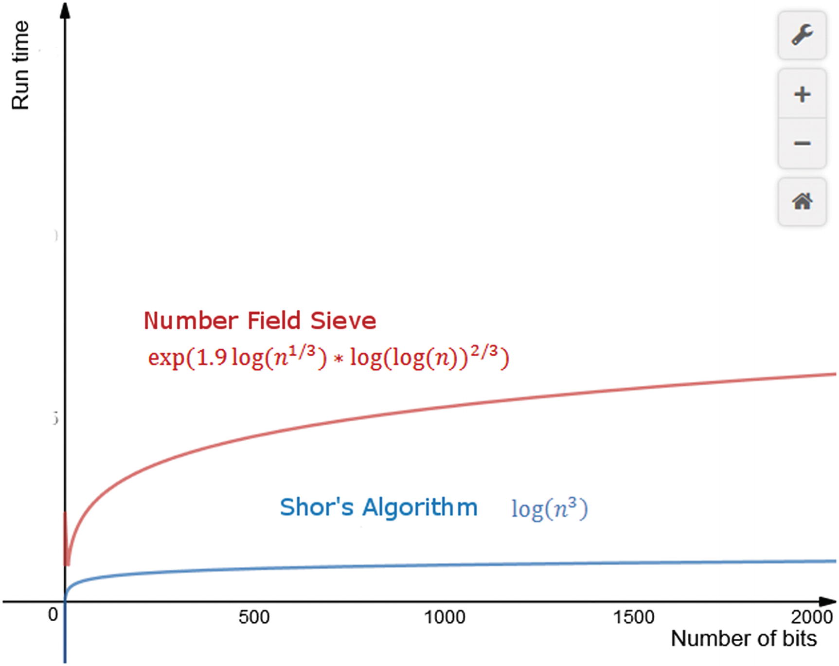
The significance of Shor’s algorithm is profound in its own right. Consider Figure 2-6 showing the time complexities of the Number Field Sieve against Shor’s algorithm.

../images/469026_1_En_2_Chapter/469026_1_En_2_Fig6_HTML.jpg — Figure 2-6
Number Field Sieve vs. Shor’s algorithm time complexity

It has been estimated mathematically that Shor’s algorithm could be able to factor a 232-digit integer (RSA-232), one of the current largest integers, in a matter of seconds. Thus a practical quantum computer that can execute Shor’s algorithm will render current asymmetric cryptography useless. Keep in mind that asymmetric cryptography is used all over society: at the bank, for example, to encrypt data and accounts, at the Web to browse, communicate, you name it.

But don’t rush to the bank, get all your money and put it under the mattress just yet. A practical implementation of this algorithm is decades away right now. This fascinating algorithm is discussed in more detail in a later chapter of this book.

Now back to Feynman and his quantum computer. In a classical computer, the basic unit is the bit (a 0 or 1). In Feynman’s computer, the basic unit is the qubit or quantum bit. A unit that is as bizarre as the theory is built upon.

The Qubit Is Weird and Awesome at the Same Time

Just like its classical cousin, the qubit can take a value of either 0 or 1. Physically, qubits can be represented as any two-level quantum systems such as

The spin of a particle in a magnetic field where up means 0 and down means 1 or
The polarization of a single photon where horizontal polarization means 1 and vertical polarization means 0. You can make a quantum computer out of light. How weird is that.

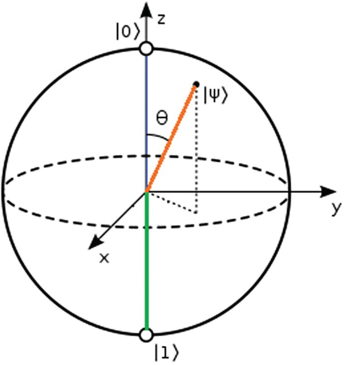
In both cases 0 and 1 are the only possible states. Geometrically, qubits can be visualized using a shape called the Bloch sphere, an instrument named after Swiss physicist Felix Bloch (see Figure 2-7).

../images/469026_1_En_2_Chapter/469026_1_En_2_Fig7_HTML.jpg — Figure 2-7
Geometrical representation of a quantum state using the Bloch sphere

Formally, the Bloch sphere is the geometrical representation in three-dimensional Hilbert space of the pure state of a two-level quantum system or qubit. The north and south poles of the sphere represent the standard basis vectors |0> and |1>, respectively; these in turn correspond to the spin-up and spin-down of the electron. Besides the basic vectors, the sphere can have something in between; this is called a superposition and it is essentially the probability for 0 or 1. The trick is that we can’t predict which it will be except at the instant of observation when the probability collapses into a definitive state.

Superposition of States

Imagine if you could flip a coin that could fall not only in a heads or tails position, but in both positions at the same time. Such a coin would be more powerful. Nevertheless there is a catch; the moment you observe this quantum coin, it is forced to take either heads or tails never knowing what position it was in before. This is one reason one needs to be careful when measuring qubits, because they change as soon as observed. All in all, superposition is a game changer. Let’s see why:

A 1-bit classical computer can be (or store) in 1 of 2 states at a time: 0 or 1. A 1-qubit quantum computer can be (or store) in 2 states at a time. That is 2¹ = 2.
A 2-bit classical computer can store only 1 out of 2² = 4 possible combinations. A 2-qubit quantum computer can store 2² = 4 possible values simultaneously.

Assuming that a byte (8 bits) is the basic unit used to store information in either system, then the number of values that can be stored simultaneously in a quantum computer would be 2ⁿ where n is the number of qubits. Compare this against the storage capacity of a classic computer (shown in Table 2-5) and you realize why qubits are powerful indeed.

Table 2-5

Qubit Simultaneous Storage Capacity

Bits/qubits	Classic storage (bytes)	Quantum storage (bits)	Quantum storage (bytes)
4	1	16	2
8	1	256	32
32	4	4294967296	536870912
64	8	1.84467E+19	2.30584E+18

Thus the amount of data that can be stored simultaneously in a quantum computer is astounding, so much so that a new term has popped up out there: quantum supremacy . This is the point at which a quantum computer will be able to solve all problems a classical computer cannot. More about this subject will be discussed in a further section of this chapter. But, for now, let’s look at the next strange property of the qubit: entanglement.

Entanglement: Observing a Qubit Reveals the State of Its Partner

Long ago, Albert Einstein called quantum entanglement Spooky action at a distance. Believe it or not, entanglement has been proved experimentally by French physicist Alain Aspect in 1982. He demonstrated how an effect in one of two correlated particles travels faster than the speed of light!

Tip

Ironically and in a sad twist of faith, humans cannot use entanglement to send messages faster than the speed of light as information cannot travel at such speed. This dichotomy, as well as Aspect’s experiment, is explained in more detail in Chapter 1.

If a set of qubits are entangled, then each will react to a change in the other instantaneously, no matter how far apart they are (in opposite sides of the galaxy, e.g., which sounds really unbelievable). This is useful in that, if we measure the properties in 1 qubit, then we can deduce the properties of its partner without having to look. Furthermore, entanglement can be measured without looking through a process called quantum tomography. Quantum tomography seeks to determine the state(s) of an entangled set prior to measurement by measurements of the systems coming from the source. In other words, it calculates the probability of measuring every possible state of the system.

Note

Multiqubit entanglement represents a step forward in realizing large-scale quantum computing. This is an area of active research. Currently, physicists in China have experimentally demonstrated quantum entanglement with 10 qubits on a superconducting circuit.⁴

Entanglement is one aspect of qubit manipulation; another mind-bending feature is manipulation via quantum gates.

Qubit Manipulation with Quantum Gates

Gates are the basic building blocks in a quantum computer. Just like their classic counterparts, they operate on a set of inputs to produce another set of outputs. Unlike their cousins however, they operate simultaneously in all possible states of the qubit which makes them really cool and weird at the same time. The basic gates of a quantum computer are:

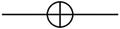
Measurement Gate

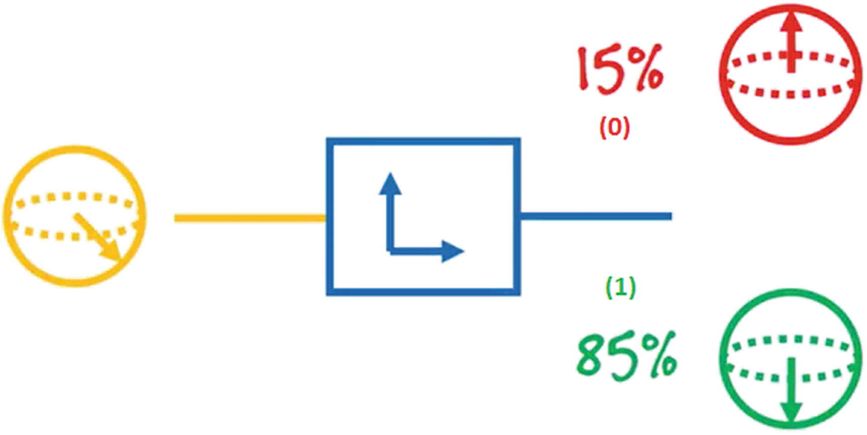
We know that the act of measuring or observing a qubit alters its state. This process is also considered a gate. The measurement gate takes a qubit in a superposition of states as input and spits either a 0 or 1. Furthermore, the output is not random. There is a probability of a 0 or 1 as output which depends on the state the qubit is originally in (see Figure 2-8).

../images/469026_1_En_2_Chapter/469026_1_En_2_Fig8_HTML.jpg — Figure 2-8
Measurement gate and its output probability

Note that the measurement gate should be the final act on a quantum circuit as quantum mechanics tells us that observing a qubit in the middle of a calculation will collapse its wave function and defeat the parallelism achieved by the superposition of states.

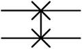
Swap Gate

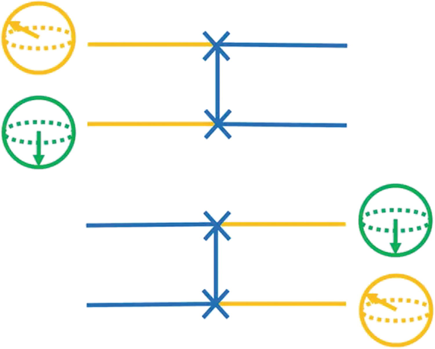
The swap gate takes 2 qubits and swaps its states as shown in Figure 2-9.

../images/469026_1_En_2_Chapter/469026_1_En_2_Fig9_HTML.jpg — Figure 2-9
Swap gate in action

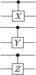
Pauli or X Gate

The Pauli gate is the quantum analog of the classic NOT gate. Formally, it rotates the qubit 180 degrees in the X-axis. Note that the X-axis points outside of the screen as shown in the Bloch sphere in Figure 2-7.

../images/469026_1_En_2_Chapter/469026_1_En_2_Fig10_HTML.jpg — Figure 2-10
Pauli X gate

Tip

The Pauli gate is named after one of the fathers of quantum physics: Austrian-born Wolfgang Ernst Pauli. In 1945 he won the Nobel Prize in Physics for developing the exclusion principle or Pauli principle which essentially says that no two electrons can exist in the same quantum state.⁵ He was highly admired by Albert Einstein and was close friends with giants of quantum mechanics: Niels Bohr and Bernard Heisenberg.

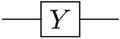
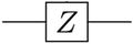
Rotation Gates: Y, Z

Rotation gates over the Y- and Z-axis are known as the Pauli Y and Pauli Z gates, respectively.

The Pauli Y gate acts on a single qubit. It rotates around the Y-axis of the Bloch sphere by π radians (180 degrees). It maps |0> to i|1> and |1> to –i|0>.
The Pauli Z gate acts on a single qubit. It rotates around the Z-axis of the Bloch sphere by π radians. It leaves the basis state |0> unchanged and maps |1> to –|1>.

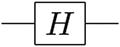
Hadamard Gate (H)

The Hadamard gate acts on a single qubit. It is the combination of two rotations:

1.
π over the X-axis
2.
π/2 over the Y-axis

The Hadamard gate is the quantum equivalent of the Hadamard matrix, a square matrix whose entries are either +1 or −1 and whose rows are mutually orthogonal.

$H=\frac{1}{\sqrt{2}}\left[\begin{array}{cc}1& 1\\ {}1& -1\end{array}\right]$

Tip

The Hadamard transform is useful in data encryption, as well as many signal processing and data compression algorithms.

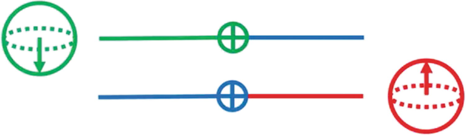
Controlled (cX cY cZ) Gates

Controlled gates act on 2 or more qubits, where 1 or more qubits act as a control for some operation. For example, the controlled NOT gate (CNOT or cX) acts on 2 qubits and performs the NOT operation on the second qubit only when the first qubit is |1> and otherwise leaves it unchanged.

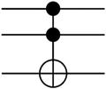
Toffoli (CCNOT) Gate

This is a controlled gate that operates in 3 qubits. If the first 2 qubits are in the state |1>, it applies a Pauli X (or NOT) on the third qubit; else it does nothing. This gate maps |a,b,c> to |a,b,c + ab>.

The quantum gates shown in Table 2-6 are the basic building blocks of quantum circuits, like the classical logic gates in Table 2-1 are for conventional digital circuits.

Table 2-6

Basic Quantum Gates

Gate name	Symbol	Details
Measurement		It takes a qubit in a superposition of states as input and spits either a 0 or 1.
X (NOT)		It rotates the qubit 180 degrees in the X-axis. Maps \|0> to \|1> and \|1> to \|0>.
Y		It rotates around the Y-axis of the Bloch sphere by π radians. It is represented by the Pauli matrix: $Y=\left[\begin{array}{cc}0& -i\\ {}-i& 0\end{array}\right]$ where $i=\sqrt{-1}$ is known as the imaginary unit.
Z		It rotates around the Z-axis of the Bloch sphere by π radians. It is represented by the Pauli matrix: $Y=\left[\begin{array}{cc}1& 0\\ {}0& -1\end{array}\right]$
Hadamard		It represents a rotation of π on the axis $\left(X+Z\right)/\sqrt{2}$ . In other words it maps the states: \|0> to $\left(\|0>+\|1>\right)/\sqrt{2}$ \|1> to $\left(\|0>-\|1>\right)/\sqrt{2}$
Swap (S)		It swaps 2 qubits with respect to the basis \|00>, \|01>, \|10>, \|11>. It is represented by the matrix: $S=\left[\begin{array}{cccc}1& 0& 0& 0\\ {}0& 0& 1& 0\\ {}0& 1& 0& 0\\ {}0& 0& 0& 1\end{array}\right]$
Controlled (cX cY cZ)		It acts on 2 or more qubits, where 1 or more qubits act as a control for some operation. Its generalized form is described by the matrix: $C(U)=\left[\begin{array}{cccc}1& 0& 0& 0\\ {}0& 1& 0& 0\\ {}0& 0& {u}_{00}& {u}_{01}\\ {}0& 0& {u}_{10}& {u}_{11}\end{array}\right]$ where U is one of the Pauli matrices σ_x, σ_y, or σ_z.
Toffoli (CCNOT)		This is a reversible gate, which means that its output can be reconstructed from its input (the states are moved around with no increase in physical entropy). It has 3-bit inputs and outputs; if the first 2 bits are both set to 1, it inverts the third bit; otherwise all bits stay the same. Reversible gates are important because they dissipate less heat. When a logic gate consumes its input, information is lost since less information is present in the output than the input. This loss of information dissipates energy to the surrounding area as heat. In quantum computing Toffoli gates are important because quantum mechanics requires transformations to be reversible and allows more general states (superpositions) of a computation than classical computers.

So a quantum gate manipulates the input of superpositions, rotates probabilities, and produces another superposition as its output. Physically, qubits can be constructed in many ways, with technology companies currently getting into the action in different directions, each design with its own strengths and weaknesses. Let’s take a look.

Qubit Design

When it comes to qubit design, only companies with big pockets can get into the race of constructing a practical quantum computer. Due to the weirdness and complexity of quantum mechanics, this is no easy task. In an article for Science Magazine⁶, writer Gabriel Popkin outlines these efforts from the titans of technology. It seems that all of them want in the action with different designs. Currently, there is no clear winner; nevertheless the race is on. According to Popkin, these are the most common types of qubits:

Superconducting Loops

When an electric current passes through a conductor, some of the energy is lost in the form of heat and light. This is called resistance, and it depends on the type of material; some metals like copper or gold are great conductors of electricity and thus have low resistance. Scientists discovered that the colder the material is, the better conductor of electricity it becomes. Thus the lower the temperature gets, the lower the resistance. Nevertheless, no matter how cold gold or copper gets, it will always show a level of resistance.

Mercury is different however. In 1911, scientists discovered that when cooling down mercury to 4.2 degrees Kelvin (above absolute zero), its resistance becomes zero. This experiment leads to the discovery of the superconductor, a material that has zero electrical resistance at very low temperatures. Since then many other superconducting materials have been found: aluminum, gallium, niobium, and others which show zero resistance at a critical temperature. The great thing about superconductors is that electricity flows without any loss, so a current in a close loop can theoretically flow forever.

Tip

This principle has been proved experimentally when scientists were able to maintain electricity flowing over superconducting rings for years.

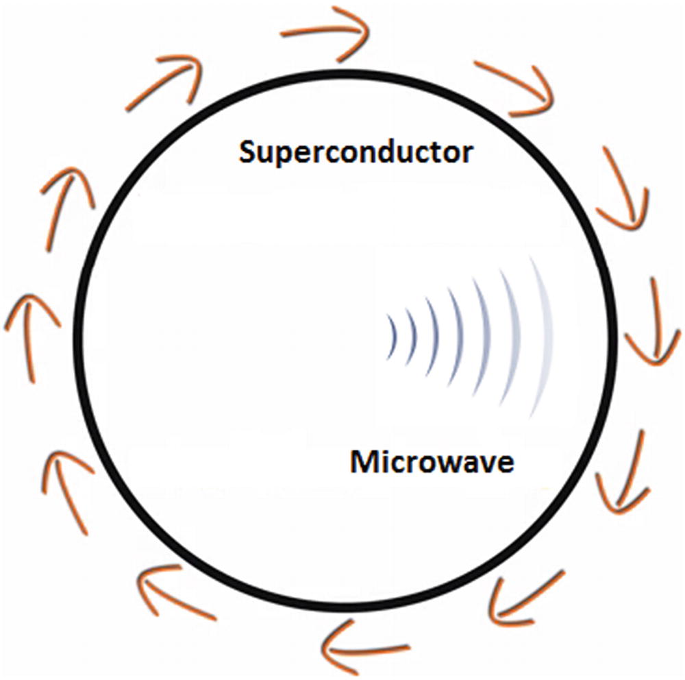
In a qubit made of a superconductor loop, a current oscillates back and forth around a loop. A microwave is injected which excites the current into a superposition of states (see Figure 2-11). Let’s look at the advantages and disadvantages of such design.

../images/469026_1_En_2_Chapter/469026_1_En_2_Fig11_HTML.jpg — Figure 2-11
Superconductor loop qubit

Pros:

Low error levels (around 99.4% logic success rates)
Fast, built on existing materials
Decent number of entangled qubits (9) capable of performing a 2-qubit operation

Cons:

Low longevity: 0.00005 s. That is, the minimum amount of time a superposition of states can be kept
Must be kept very cold, at a super frosty –271 °C

This design is used by IBM’s cloud platform Q Experience which is the basis for the code used in this book. It is also used by Google and a private venture called Quantum Circuits, Inc. (QCI) which seeks to manufacture a practical quantum computer based on superconductors .

Trapped Ions

An ion trap is a technique for controlling quantum states in a qubit. It uses a combination of electric or magnetic fields to capture charged particles (ions) in a system isolated from the external environment. Lasers are applied to couple qubit states for single operations or coupling between the internal states and the external motional states for entanglement.

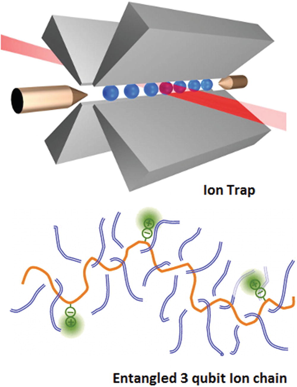
Ion traps seek to realize the dream of large-scale universal quantum computing by scaling with arrays of ion traps. This technique is also capable of building large entangled states via photonically connected networks of remotely entangled ion chains or combinations of these two ideas (see Figure 2-12).

../images/469026_1_En_2_Chapter/469026_1_En_2_Fig12_HTML.jpg — Figure 2-12
Ion traps and chains for large-scale quantum computing

Let’s look at the pros and cons of trapped ions:

Pros:

High longevity: Experts claim that trapped ions can hold entanglement for up to 1000 s which is huge compared to superconductor loops (0.00005 s).
Better success rates (99.9%) than superconductors (99.4%). Not much, but still.
Highest number so far (14) of entangled qubits capable of performing a 2-qubit operation.

Cons:

Slow operation. Requires lots of lasers.

The top company developing this technology is IonQ located in Maryland, USA.

Silicon Quantum Dots

Intel, the juggernaut of the PC CPU, is spearheading this design. In a silicon quantum dot, electrons are confined vertically to the ground state of a quantum gallium arsenide (GaAs) well, forming a two-dimensional electron gas (2DEG). A 2DEG electron gas is free to move in two dimensions, but tightly confined in the third (see Figure 2-13). This tight confinement leads to quantized energy levels for motion in the third direction which may be of high interest in quantum-based structures.

Tip

2DEG are currently found on transistors made from semiconductors. They also exhibit quantum effects such as the Hall effect, in which a two-dimensional electron conductance becomes quantized at low temperatures and strong magnetic fields.

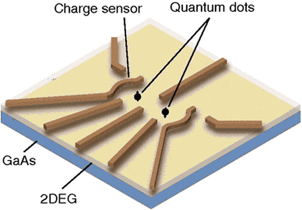
../images/469026_1_En_2_Chapter/469026_1_En_2_Fig13_HTML.jpg — Figure 2-13
Quantum dot made of gallium arsenide

The pros and cons of silicon quantum dots are

Pros:

Stable, built on existing semiconductor materials
Better longevity than superconductor loops, at 0.03 s

Cons:

Low number of entangled qubits (2) capable of performing a 2-qubit operation
Lower success rate than superconductor loops or trapped ions, but still high at 99%

Topological Qubits

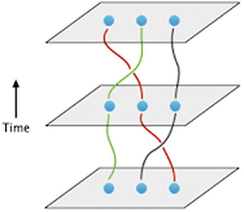
Topological qubits seek to eliminate error levels characteristic of quantum computers. Errors are due to the probabilistic nature of quantum mechanics and are described by the longevity or the duration of qubit entanglement. A topological qubit uses two-dimensional quasiparticles called anyons whose paths pass around one another to form braids in a three-dimensional space-time. These braids form the logic gates that make up the computer.

../images/469026_1_En_2_Chapter/469026_1_En_2_Fig14_HTML.jpg — Figure 2-14
Topological qubit with braids acting as logical gates

Pros:

Stable, error-free (longevity doesn’t apply)

Cons:

Purely theoretical at this point, although recent experiments indicate these elements may be created in the real world using semiconductors made of gallium arsenide at a temperature near absolute zero and subject to strong magnetic fields

Microsoft and Bell Labs are some of the companies that support this design.

Diamond Vacancies

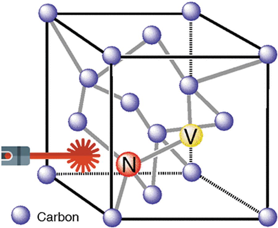
Diamond vacancies are locations in the diamond’s crystal lattice where there should be a carbon atom but there isn’t one. Diamond vacancies seek to harness nanometer-scale atomic defects in diamond materials to function as qubits. It has been observed using atomic force microscopy that the surface of natural diamonds reveals several types of defects. This defect, or vacancy, along with a Nitrogen atom adds an electron to a diamond lattice. The electron quantum spin can then be controlled with a laser as shown in Figure 2-15.

../images/469026_1_En_2_Chapter/469026_1_En_2_Fig15_HTML.jpg — Figure 2-15
Diamond vacancy qubit

According to Dirk Englund and colleagues at the MIT School of Electrical Engineering and Computer Science, diamond vacancies solve the perennial problem of reading information out of qubits in a simple way. Diamonds are natural light emitters, and as so, the light particles emitted by diamond vacancies preserve the superposition of states, so they could move information between quantum computing devices. Best of all, they work at room temperatures. No need to cool things down to –272 degrees!

One pitfall of diamond vacancies, says Englund, is that only about 2% of the surface of the diamond has them. Nevertheless researchers are developing processes for blasting the diamond with beams of electrons to produce more vacancies.

Pros:

High longevity: 10 s.
High success rate: 99.2%.
Decent number of entangled qubits (6) capable of performing a 2-qubit operation.
Qubits operate at room temperature. How incredible is that.

Cons:

Small number of vacancies in surface materials: about 2%
Difficult to entangle

All in all, quantum computers have come a long way since the days of Richard Feynman with some of the world’s biggest companies looking to cash in. Right now superconductor loops are leading the pack. However there are amazing new designs, such as diamond vacancies, that seek to realize the dream of large-scale quantum computing.

Quantum Computers vs. Traditional Hardware

Quantum computers outmuscle classical hardware for certain tasks. Consider Table 2-7 showing the time complexities for two specific tasks of a quantum vs. a classical computer.

Table 2-7

Quantum vs. Classical Time Complexities for Certain Tasks

Task	Quantum	Time complexity	Classical	Time complexity
Search	Grover’s algorithm	$\sqrt{n}$	Quick search	n/2
Large integer factorization	Shor’s algorithm	log(n³)	Number Field Sieve	$\exp \left(1.\mathrm{9log}\left({n}^{\frac{1}{3}}\right)\ast \log {\left(\log (n)\right)}^{\frac{2}{3}}\right)$

For search, Grover’s algorithm provides better performance than traditional search. This can have a profound impact in the data center for companies like Google, MS, and Yahoo. Imagine your web search powered by quantum processors in the cloud. We are long ways from that right now, but still. This is one of the reasons big tech companies are investing heavily in developing their quantum platforms.

Another task, and perhaps the main reason why quantum is picking up such steam, is large integer factorization. When Peter Shor came up with his quantum factorization algorithm, he punched a serious crack at the cryptographic security that is at the foundation of our society. Shor’s algorithm threatens current encryption systems by factorizing large integers quickly. These integers are used to create the cryptographic keys to encode all data in the Web: bank accounts, business transactions, chats, cat videos, you name it. Shor’s algorithm is so fast that, in fact, it could factorize the largest integers of todays in a matter of minutes. Compare that with the current classical champ, the Number Field Sieve, which may take billions of years to factorize such numbers.

Besides search and cryptography, quantum computers can be invaluable tools for simulations, molecular modelling, artificial intelligence, neural networks, and more. Let’s see how.

Complex Simulations

Physicists agree that simulations at the atomic level are the field where quantum machines excel. It is the perfect fit after all; a machine built around atoms would be able to simulate quantum mechanical systems with a much greater accuracy than a classical computer. It has been estimated that a quantum computer with a few tens of quantum bits could perform simulations that would take an unfeasible amount of time on a classical computer. For example, the Hubbard model, named after British physicist John Hubbard, which describes the movement of electrons within a crystal, can be simulated by a quantum computer.⁷ According to Hubbard, this is a task that is beyond the powers of a classical computer.

Molecular Modelling and New Materials

According to an article in Science Magazine, theoretical chemists at the Italian Institute of Technology in Genoa have modelled a molecule of beryllium hydride,⁸ a small compound made of two hydrogen and one beryllium atom, in a quantum computer. Not a big deal by today’s classical standards but nevertheless a stepping-stone in a future full of hope for new drug discoveries.

Molecular modelling is a virgin new field for quantum machines as physicists and chemists routinely use computers to simulate how atoms and molecules behave. Mathematicians claim that most simulations require massive amounts of computing power. This is especially true for molecular simulations due to the interactions of particles that become exponentially more complex as their numbers increase. Plus the weird laws of quantum mechanics make it hard to calculate the distribution of these electrons within a molecule. Table 2-8 shows some of the current experiments in this field.

Table 2-8

Quantum Experiments in Molecular Modelling

Year	Company	Experiment
2016	Google	Researchers at the quantum computing lab in Venice, California, used 3 qubits to calculate the lowest energy electron arrangement of a molecule of hydrogen.
2017	IBM	IBM develops an interactive algorithm to calculate the ground state of specific molecules. Scientists used up to 6 superconductor qubits to analyze hydrogen, lithium hydride, and beryllium hydride by encoding each molecule’s electron arrangement into the quantum computer and nudge the molecule into its ground state which they measured and encoded onto a conventional computer.

All in all, molecular modelling has a modest start, but still the future looks bright for chemistry and drug companies. Molecular simulation looks to be a killer application for quantum computing.

Sophisticated Deep Learning

When it comes to deep learning traditional problems fall into three categories: simulation, optimization, and sampling. We have seen in previous sections how a quantum computer excels at simulations, especially at the molecular and atomic levels, but what about optimization? Some optimization problems are not feasible in traditional hardware due to the extreme numbers of interacting variables required to solve them. Examples of these problems include protein folding, space craft flight simulations, and others. Quantum computers can tackle optimization efficiently using a technique called stochastic gradient descent . This is a technique for searching for the best solution among a large set of possible solutions, comparable to finding the lowest point on a landscape of hills and valleys.

Tip

As a matter of fact, a Canadian company called D-Wave already sells commercial quantum computers specifically designed to tackle optimization problems using stochastic gradient descent and other techniques. Some of their customers include defense contractor Lockheed Martin and Google.

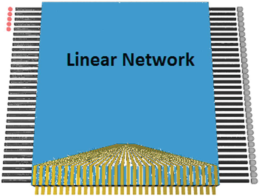
Quantum sampling problems fall under the set of computational problems that produce samples from probability distributions. Two classes of sampling problems that demonstrate the power of quantum algorithms are Boson sampling and instantaneous quantum polynomial time sampling. Several small-scale implementations of these two techniques have been performed with quantum optics.

../images/469026_1_En_2_Chapter/469026_1_En_2_Fig16_HTML.jpg — Figure 2-16
Schematic of the Boson sampling problem

Figure 2-16 shows a schematic of the Boson sampling problem for a 32 mode instance. Five photons (left) are injected into a linear network that has a scattering matrix (bottom), and all outputs are detected in the Fock basis (right). According to an article in the “Quantum Information” section of Nature by A. P. Lund, Michael J. Bremner, and T. C. Ralph, this problem is intractable for classical computers, even for medium-scale systems, such as 50 bosons in 2500 paths. Not even for smaller systems (20 bosons and 400 paths) a feasible classical algorithm is known which can perform this simulation.⁹

Not so much for quantum sampling problems though, which provide a path toward experimental demonstration of the supremacy of quantum algorithms in this field. Deep learning and artificial intelligence are two disciplines that go hand in hand in advanced computation with neural nets being the crown jewel of current research.

Quantum Neural Networks (QNN) and Artificial Intelligence (AI)

Quantum neural networks are the stuff of science fiction more than science fact right now. Nevertheless, the theoretical foundation has been there since the 1990s, and there is wide spread research being done in many directions including

The use of quantum information processing to improve existing neural network models¹⁰: It is all about boosting existing models with faster and more efficient algorithms. This is a field where quantum computation shines. The motivation for this research is the difficulty to train classical neural networks, especially for big data applications. The hope is that features of quantum computing such as parallelism or the effects of interference and entanglement can be used as resources.
Potential quantum effects in the brain¹¹: This path merges quantum physics and neuroscience with a vibrant debate beyond the borders of science. There are pioneers hard at work in the mostly theoretical field of quantum biology which has been gaining momentum by discoveries such as
- Signs of efficient energy transport in photosynthesis due to quantum effects
- Reports of “Mag-Lag” effects in MRI scanner patients suggesting that delicate interactions in the brain may be quantum in nature
Quantum associative memory : This is a new algorithm introduced by Dan Ventura and Tony Martinez in 1999.¹² They propose a circuit-based quantum computer that simulates associative memory. The algorithm writes memory states into superpositions, and then it uses a Grover-like quantum search to retrieve the memory state closest to a given input with the ultimate goal being to simulate features of the human brain.
Black holes : Believe it or not, ideas have been proposed about modelling black holes as QNNs and that black holes and brains may store memories in similar ways.¹³

All in all, if a SkyNet-like AI quantum computer is to enslave humanity in the future, chances are that it will be made of some sort of a QNN. It may sound like a joke right now, but giants of science such as Stephen Hawking have warned about this. We should be wise to listen. In the next section we look at the pitfalls that make quantum computers hard to build.

Pitfalls of Quantum Computers: Decoherence and Interference

Decoherence and interference are basic principles in quantum mechanics that cause trouble for large-scale quantum computing.

Decoherence (Longevity)

In quantum mechanics, particles are described by the wave function. A fundamental property of quantum mechanics is called coherence or the definite phase relation between states. This coherence is necessary for the functioning of quantum computers. However, when a quantum system is in contact with its surroundings, coherence decays with time, a process called quantum decoherence. Formally, decoherence is the time that takes for the superposition of states to disappear and is due to the probabilistic nature of the wave function. It can be viewed as the loss of information from a system into the environment.

Tip

Decoherence was introduced to understand the collapse of the wave function by German physicist H. Dieter Zeh in 1970.¹⁴

Decoherence can be tested experimentally: quantum mechanics says that particles can be in multiple states (not excited vs. excited or in two different locations) at the same time. Only the act of observation gives a random value for a particular state. If the excitation is measured by the energy levels of the particle (where low energy level means not excited and high energy means excited), when an electromagnetic wave is sent to the particle at a proper frequency, the particle will alternate between high and low energy levels. The state of the particle can then be measured and averaged producing what is called Rabi oscillations. Because the particle is never completely isolated due to atom collisions, electromagnetic fields, or thermal baths, for example, the superposition will stop and the oscillations will disappear.

Thus decoherence gives information about the interaction of a quantum object and its environment and it is crucial for quantum computing. That is, the higher the decoherence (the time it stays in superposition), the higher the quality of the qubit will be. Some qubit designs like superconductor loops have very low longevity and need to be kept at extremely low temperatures (-271 °C) to counter this effect. Others like trapped ions and diamond vacancies have very high longevity and can be kept at room temperatures. Technology companies working in quantum designs face a daunting challenge trying to wrestle with qubit longevity. For a more detailed description of these efforts, see the section under “Qubit Design.”

Quantum Error Correction (QEC)

Quantum error correction seeks to achieve fault-tolerant quantum computation by protecting information from errors due to decoherence and other environmental noise. When a quantum computer sets up some qubits, it applies quantum gates to entangle them and manipulate probabilities and then finally measures the output collapsing superpositions to a final sequence of 0s or 1s. This means that you get the entire lot of calculations with your circuits done at the same time. Ultimately, you can only measure one output from the entire range of possible solutions. Every possible solution has a probability to be correct so it may have to be rechecked and tried again. This process is called quantum error correction.

In the classical world, error correction is done with redundancy, that is, by creating copies of the data and then assigning probabilities to the possible error conditions and finally comparing the highest probable condition with the original message to determine if an error has occurred. To illustrate this process, consider the following table representing one bit of information:

Message	Redundant copies	Error (1)	Error (1,2)
0	0	1	1
	0	0	1
	0	0	0
Probability		(1/3) = 0.33	(1/3)*(1/3) = 0.11

Let’s say that we have a 1 bit message (0) and we create three redundant copies for error correction. Assuming that noisy errors are independent and occur with some probability, it is more likely that the error occurs in a single bit and the transmitted message is three 0s. It is also possible that a double-bit error occurs and the transmitted message is equal to three 1s, but this outcome is less likely. Thus we can use this method to correct the message in case of errors in a classical system. Unfortunately, this is not possible at quantum scales due to the no-cloning theorem.

Note

The no-cloning theorem states that it is impossible to create an identical copy of an arbitrary unknown quantum state. It was postulated and proved by Physicist James L. Park in 1970.¹⁵

The no-cloning theorem creates trouble for quantum computing as redundant copies of qubits cannot be created for error correction. Nevertheless it is possible to spread the information of 1 qubit onto a highly entangled state of several physical qubits . This technique was discovered by Peter Shor with a method of error correcting code by storing the information of 1 qubit onto 9 entangled qubits. However, this scheme only protects against errors of a limited form. Over time several schemes of quantum error correction codes have been developed. The most important are:

The 3-Qubit Code

This is the most basic and the starting point for quantum error correction. This method encodes a single logical qubit into three physical ones with the property that it can correct a single bit-flip error in the Pauli X matrix (σ_x). This code is able to correct errors without measuring the state of the original qubit by using 2 extra qubits to extract what is called syndrome information (information regarding possible errors) from the data block without disturbing the original state.

The caveat of this code is that it cannot correct for both bit and phase (sign) flips simultaneously, only a single bit flip. Peter Shor used this method to develop a 9-qubit error correction code.

Shor’s Code

This error correction code is based on the 3-qubit code, and it is capable of correcting bit flips, sign flips, or both simultaneously. Shor’s code works by encoding 1 single logical qubit into 9 physical qubits using this extra real state to store syndrome information about the possible errors. Note that this code can correct errors in a single qubit only. This code tends to be simpler, allowing for more cooperative circuit structures to the physical restrictions of computer architecture. Furthermore, other modern developments in quantum error correction include

Bosonic codes : These try to store error correction information in bosonic modes using the advantage that oscillators have infinitely many energy levels in a single physical system.¹⁶
Topological codes : These were introduced by physicist Alexei Kitaev with the development of his toric code for topological error correction. Its structure is defined on a two-dimensional lattice using error chains which define nontrivial topological paths over the code surface.¹⁷

All in all, decoherence and quantum error correction are not making things easy for IT companies seeking to realize the dream of large-scale fault-tolerant quantum computing. Nevertheless progress continues at a rapid pace thanks to new qubit designs with high levels of longevity and improved quantum error correction codes. In fact, the pace is so quick that experts in the field have coined a new catchy term for large-scale quantum computing: quantum supremacy.

The 50-Qubit Processor and the Quest for Quantum Supremacy

Quantum supremacy is a catchy term indeed. It was coined by physicist John Preskill to describe the point at which a quantum computer could solve problems that classical computers cannot. This is a very potent claim as it requires proof of super-polynomial speedups over their best classic counter parts.

Tip

A super-polynomial speedup is an improvement in the execution of an algorithm above the bounds of a polynomial. For example, an algorithm that runs at k1n^c1 + k2n^c2 +… where k and c are arbitrary constants and n is the size of the input is said to be of polynomial time. An algorithm that runs at 2ⁿ where n is the size of the input is said to be of super-polynomial time.

Researchers are hard at work on proving quantum supremacy with a few algorithms already in place that provide super-polynomial speedup over the classic champs. The following paragraphs detail a timeline of these efforts.

1982: Richard Feynman, the titan of quantum mechanics, proposes a quantum computer that can take advantage of the atomic principles of superposition, interference, and entanglement. Such a machine will be a game changer.
1994: Mathematician Peter Shor comes up with his notorious factorization algorithm for a quantum computer. The algorithm becomes a sensation when it is estimated that its time complexity crushes the classical super champ (the Number Field Sieve - NFS) by super-polynomial speedups. The algorithm has neither been implemented nor proved experimentally; nevertheless, the genie is out the bottle as excitement grows almost as fast as Shor’s algorithm speedup over NFS.
2012: Physicist John Preskill coins the term quantum supremacy in the paper “Quantum Computing and the Entanglement Frontier” to formally describe the point in time at which quantum computers will take over. The race is on among the giants of information technology.
2016: Google, the search giant, decides to take on the challenge of proving quantum supremacy by the end of 2017 by constructing a 49-qubit chip that will be able to sample distributions inaccessible to any current classical computers in a reasonable amount of time. The effort fails.
2017: Researchers at IBM T. J. Watson lab perform a simulation of 49- and 56-qubit circuits on a conventional Blue Gene/Q supercomputer at the Lawrence Livermore National Laboratory, increasing the number of qubits needed for quantum supremacy.¹⁸
2018: Skepticism grows on proving quantum supremacy as the pitfalls of quantum computing become more apparent: quantum error correction estimates get as high as 3% of the input on each cycle. Quantum computers are much noisier and error prone compared to their classical counter parts. The Holy Grail becomes a fault-tolerant quantum computer.

Although quantum supremacy is still a long way before a definitive proof, IT insiders predict companies will start seeing returns on their investment into quantum within a few years. Whenever or under which qubit count this so-called quantum supremacy arrives, not even supercomputers will be able to keep up. Believe it or not, there is a company in Canada called D-Wave Systems selling 2000-qubit computers commercially. Although their work remains controversial due to the use of a process called quantum annealing. The next section shows why.

Quantum Annealing (QA) and Energy Minimization Controversy

Quantum annealing sometimes called adiabatic quantum computation (AQC) is a form of quantum computing that relies in the adiabatic theorem to perform calculations. Without getting too technical, here is a list of concepts to better understand this process:

Adiabatic theorem : It was postulated by Max Born and Vladimir Fock in 1928 and states: A quantum mechanical system subjected to gradually changing external conditions adapts its functional form, but when subjected to rapidly varying conditions there is insufficient time for the functional form to adapt, so the spatial probability density remains unchanged.
Hamiltonian (H) : An important concept in quantum mechanics especially so for quantum annealing. In quantum mechanics, a Hamiltonian is an operator corresponding to the total energy of the system in most of the cases. In other words, it is the sum of the kinetic energies of all the particles, plus the potential energy of the particles associated with the system.

Tip

The adiabatic theorem is better understood by a simple example of a pendulum oscillating in a vertical plane. If the support of the pendulum is moved abruptly, the mode of oscillation of the pendulum will change. On the other hand, if the support is moved very slowly, the motion of the pendulum relative to the support will remain unchanged. This is the essence of the adiabatic process: A gradual change in external conditions allows the system to adapt, such that it retains its initial character.

In general terms, quantum annealing can be described by the following steps:

1.
Find a potentially complicated Hamiltonian whose ground state describes the solution to the problem of interest.
2.
Prepare a system with a simple Hamiltonian and initialize to the ground state.
3.
Use an adiabatic process to evolve the simple Hamiltonian into to the desired complicated Hamiltonian. By the adiabatic theorem, the system remains in the ground state, so at the end the state of the system describes the solution to the problem.

The pioneer in this form of quantum computing is a company called D-Wave Systems which has sold commercially several quantum computers with fairly large numbers of qubits.

2000 Qubits: Things Are Not As They Seem

Consider the following timeline for a series of quantum systems commercially sold by D-Wave.

2007: D-Wave demonstrates their first 16-qubit hardware.
2011: D-Wave One, a 128-qubit computer sold to Lockheed Martin for 10 million USD.
2013: D-Wave Two, a 512-qubit computer sold to Google for their Quantum Artificial Intelligence Lab seeking to prove quantum supremacy.
2015: D-Wave 2X, breaks the 1000-qubit barrier when sold to an unknown partner.
2017: D-Wave 2000Q, their latest 2000-qubit computer sold to a cybersecurity firm called Temporal Defense Systems for 15 million USD.

It may seem hard to believe that a 2000-qubit quantum computer has already been sold when giants like IBM and Google are just beginning to build 16-qubit systems. Considering that IBM is a company that specializes in large-scale hardware and has the deepest pockets of anybody out there. They would not simply let this happen. Well, the truth is that, in spite of the large number of qubits of the D-Wave 2000Q, it cannot tackle most of the problems that the IBM Q system can.

As a matter of fact, a D-Wave computer can only solve quantum annealing problems, that is, problems solvable by the adiabatic theorem.

Quantum Annealing: A Subset of Quantum Computing

Quantum annealing has been called restrictive by experts in the field generating some controversy due to the following facts:

Platform like IBM Q use logic gates to control the qubits, while quantum annealing computers don’t have logic gates and therefore cannot fully control the state of the qubits.
D-Wave Systems leverage the fact that their qubits tend to a minimum energy state. They cannot be controlled via quantum gates but their behavior can be predicted by the adiabatic theorem. This makes them good tools for solving energy minimization problems .
Quantum annealing is used mainly for combinatorial optimization problems where the search space is discrete with a local minimum (e.g., finding the ground state of a disordered magnet/spin glass).¹⁹ QA takes advantage of the notion that all physical systems tend toward a minimum energy state. To illustrate this, take a hot cup of coffee; when left over the counter for some time, it will start to cool down until it reaches a temperature equal to the surrounding environment. Thus, it tends toward a minimum energy state.

Tip

Mathematical optimization is a technique from the family of local search. It is an iterative method that starts with an arbitrary solution to a problem and then attempts to find a better solution by incrementally changing a single element of the solution. If the change produces a better solution, an incremental change is made to the new solution, repeating until no further improvements can be found.

The question of whether or not the D-Wave QA machine can outmuscle classical computers remains unanswered with several studies going either way: in January 2016, scientists at Google used a D-Wave system to perform a series of tests on finite-range tunnelling of a QA solver against simulated annealing (SA) and simulated quantum Monte Carlo (QMC) on a single-core classical processor.²⁰ Their results: The QA solver outperformed SA and QMC by a factor of 10⁸.

Pretty impressive, however others have said not so fast: Researchers from the Swiss Federal Institute of Technology claimed no quantum speedup for the D-Wave chip but didn’t rule out that there could be one in the future.

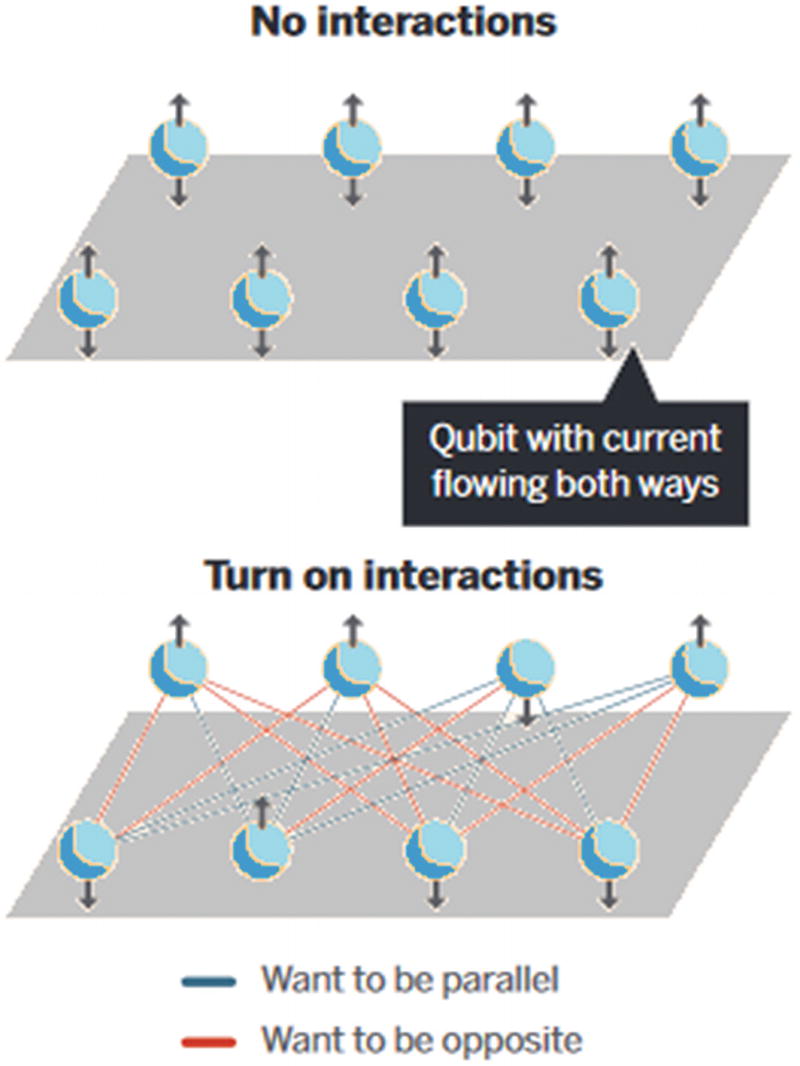
Figure 2-17 shows the basic inner workings of QA processor such as D-Wave’s. It consists of a 2D array of qubits made of superconducting loops which carry an electric current. The qubits act like magnets that can point up, down, or by the properties of quantum mechanics up and down at the same time. Each qubit in the array can interact with others through linkers that can be programmed so that they can lower their energy by either pointing in the same or opposite direction. The idea is to encode a problem by specifying all possible interactions in the chip and solve it by finding the qubit’s lowest energy or ground state.

../images/469026_1_En_2_Chapter/469026_1_En_2_Fig17_HTML.jpg — Figure 2-17
Schematic of a quantum annealing processor

To find the ground state, the machine starts the array in an entangled state and slowly turns on the interactions. The system then seeks the lowest energy state like a ball rolling thru a valley of peaks to find the deepest point. In classical physics the jiggling of thermal energy drives the ball through the valley to a low point; this is called thermal annealing . In quantum mechanics however, the ball can tunnel through low spots to find the lowest even faster. This is the reason why quantum annealing is believed to be faster for problems such as pattern recognition or machine learning.

Thus D-Wave’s architecture differs from traditional quantum computers in that it can only solve energy minimization problems . This has created a level of controversy with some at IBM calling it “a dead end.” Even the scientists at Google that performed the QA experiment in the D-Wave 2X for instances of K^th order binary optimization quip in their summary that simulated annealing is for the “ignorant or desperate.” Adding to the controversy is the fact that D-Wave cannot execute Shor’s algorithm because it is not an energy minimization process. Shor’s requires what is called a universal quantum computer, a computer that can execute any quantum algorithm.

Universal Quantum Computation and the Future

A universal quantum computer also known as a quantum Turing machine (QTM) is the ultimate quantum machine. It has been defined as an abstract machine capable of seizing all the power of quantum computation. That is, capable of executing any quantum algorithm. Although we are decades away from realizing this dream, a new global race has begun with both major IT industry players and governments pouring significant resources into R&D for these machines.

Google and Quantum Artificial Intelligence

Google has been an early customer of D-Wave and used their machines on a series of optimization experiments whose results showed that quantum annealing can be significantly faster than simulated annealing on a single-core processor. Furthermore, Google has announced that it is developing its own quantum computing technology, a move that makes perfect sense given the amount of resources at their command. Although nothing is available for demonstration at this time, it appears to be a hybrid between IBM’s gate-based approach and D-Wave’s quantum annealing.

As a matter of fact, Google announced in June 2017 that they are testing a 20-qubit quantum computer with hopes of building a 49-qubit machine by 2018. It seems that they want to give IBM a run for its money in the quest for quantum supremacy. Google has made their quantum wishes clear: artificial intelligence. In the paper “Commercialize Early Quantum Technologies” for Springer Nature, they present the Quantum AI Laboratory with the purpose of building a fault-tolerant quantum machine that can tackle any problem. Google’s efforts focus in three key areas of machine learning and artificial intelligence:

Simulation: One of the most anticipated applications is modelling of chemical reactions and materials: stronger polymers for aircraft, improved catalytic converters for cars, more efficient materials for solar, new pharmaceuticals, and breathable fabrics. Quantum computing promises to save untold amounts of money by taking the computer power required to create these materials to the next level. Computational materials are a large industry with a variety of business models built for quantum simulation: pay a subscription for access, consulting, equity exchange in return for quantum-assisted innovations, and others.
Optimization: Optimization problems are difficult to solve with conventional computers. The best classical methods use statistical methods such as energy minimization (thermal annealing). Quantum principles can provide significant speedups by tunnelling thru the thermal barriers in order to find the lowest possible point or best solution. Online recommendations and bidding strategies for advertisements are some of the tasks that require powerful optimization algorithms. In general most machine learning problems can benefit from quantum optimization. Logistics companies, patient diagnosis in health care, and web search companies could achieve tremendous innovation.
Sampling: Mostly related to machine learning tasks such as inference and pattern recognition. Quantum sampling can provide superior performance in probability distribution queries. Not only that, but the massive parallelism achieved by quantum computers can use sampling to provide definitive proof of quantum supremacy.

Google is betting heavily in the future of quantum optimization and risk management, but for now IBM has the advantage with their 20-qubit platform for commercial customers and a 16-qubit free for all cloud platform – the Q Experience. One thing is for sure ; expect to see cloud-based quantum platforms from every major vendor soon.

Quantum Machines in the Data Center

Qubit design and construction is based on extreme engineering. Because of the bizarre nature of quantum mechanics , qubits are highly susceptible to noise from the environment, error prone due to the principle of decoherence, and in general hard to control and build at a large scale. Thus don’t expect quantum computers at the counter of the local Best Buy any time soon. Don’t expect either that in the next decades your grandson will be able to buy a quantum computer and plug it in the middle of the family room. Unless a quantum leap in technology is achieved, this is unlikely to happen at all. This is in part because current qubits must be kept at ultrafrosty 0.015 K or around –273 °C to avoid noise from the environment. To have some perspective of this temperature, consider the following table showing average temperatures for different regions of the universe.

Location	Temperature Kelvin	Temperature Celsius
Qubit	0.015	–273
Vacuum of space (the temperature produced by the uniform background radiation or afterglow from the Big Bang)	2.7	–270
Average temperature of earth	331	58
Temperatures of the moon at daytime and night	373/100	100/–173

Tip

Kelvin is the primary unit of temperature in physics. Zero Kelvin is defined as the absolute zero or the temperature at which all thermal motion ceases in the classical description of thermodynamics.

What is very likely to happen in the short term is that quantum computers will take over the data center. This means quantum computers will not replace the desktop, but instead perform most of the heavy-duty tasks in the data center such as search, simulations, modelling, and others. Furthermore insiders expect that quantum computers will complement traditional computers offering new types of services such as encryption, scientific intelligence, and artificial intelligence.

So, in a few years, expect the digital assistant in your phone or at home to be powered by a quantum computer. Here is some food for thought: In a decade or so, we will spend most of our time talking to quantum computers.

The Race Is Going Global

Things reach a new level when entire governments get into the action with heavy investments in the field. According to a press release by Digital Single Market, the European Commission is planning to launch a €1 billion flagship initiative starting in 2018 with substantial funding for the next 20 years.²¹ This is a follow-up investment in addition to the €550 million spent on individual initiatives in order to put Europe at the forefront of what they consider the second quantum revolution.

Furthermore, according to a press release by Alibaba Cloud in July 2015, the Chinese Academy of Sciences (CAS) is teaming up with Alibaba, the largest e-commerce player in China to create the CAS Quantum Computing Laboratory. Quantum computing has turned into a global race and the implications will be profound.

Future Applications

There is no limit to the things that can be achieved by the tremendous potential of quantum computing. Here is a list of possible future applications and their impact in our society.

Aircraft industry : Aircraft companies are working in developing and using quantum algorithms for airflow simulations shaving years over their classical counterparts. This will result in more robust and efficient aircraft with low noise and emissions in a fraction of the time.
Space applications : NASA has been toying with the D-Wave system for tasks ranging from optimal structures to optimal packing of payload in a space craft. Other applications include quantum artificial intelligence algorithms and quantum-classical hybrid algorithms.
Medicine : Quantum computing can provide superior molecular simulations resulting in new medicines, lightning fast protein modelling, and faster drug testing. This will reduce the life cycle used to bring medicine to the patient. Next-generation drugs and cancer cures are at our grasp.

These are just some of the future applications of quantum computing. Note that we do not include current breakthroughs such as data encryption and security: quantum factorization and the possibility of defeating asymmetric cryptography are arguably the main reasons quantum computing has picked up so much steam lately. In the next chapter you will get your feet wet with the IBM Q Experience. This is the first quantum computing platform in the cloud that provides real quantum devices for use at our hearts’ desire.

Footnotes

Engel, Thomas. Quantum Chemistry and Spectroscopy. Upper Saddle River, NJ. Pearson, 2006. Print.

Quantum computation. David Deutsch, Physics World, 1/6/92. A comprehensive and inspiring guide to quantum computing.

Peter W. Shor. Polynomial-Time Algorithms for Prime Factorization and Discrete Logarithms on a Quantum Computer. https://arxiv.org/abs/quant-ph/9508027

Chao Song et al. “10-Qubit Entanglement and Parallel Logic Operations with a Superconducting Circuit.” Physical Review Letters. DOI: 10.1103/PhysRevLett.119.180511.

Nobel Lecture: Exclusion Principle and Quantum Mechanics Pauli’s own account of the development of the Exclusion Principle. www.nobelprize.org/nobel_prizes/physics/laureates/1945/pauli-lecture.html

“Scientists are close to building a quantum computer that can beat a conventional one.” http://www.sciencemag.org/news/2016/12/scientists-are-close-building-quantum-computer-can-beat-conventional-one

Hubbard, J. (1963). “Electron Correlations in Narrow Energy Bands”. Proceedings of the Royal Society of London. 276 (1365): 238–257. Bibcode:1963RSPSA.276..238H. doi:10.1098/rspa.1963.0204. JSTOR 2414761

“Quantum computer simulates largest molecule yet” By Gabriel Popkin Sep. 13, 2017 available at http://www.sciencemag.org/news/2017/09/quantum-computer-simulates-largest-molecule-yet-sparking-hope-future-drug-discoveries

A. P. Lund, Michael J. Bremner and T. C. Ralph. Quantum sampling problems, BosonSampling and quantum supremacy. Available at www.nature.com/articles/s41534-017-0018-2

M. Schuld, I. Sinayskiy, F. Petruccione: The quest for a Quantum Neural Network, Quantum Information Processing 13, 11, pp. 2567-2586 (2014).

W. Loewenstein: Physics in mind. A quantum view of the brain, Basic Books (2013).

D. Ventura, T. Martinez: A quantum associative memory based on Grover’s algorithm, Proceedings of the International Conference on Artificial Neural Networks and Genetics Algorithms, pp. 22-27 (1999).

Black Holes as Brains: Neural Networks with Area Law Entropy. Gia Dvali and colleagues. Available at https://arxiv.org/pdf/1801.03918.pdf .

Schlosshauer, Maximilian (2005). “Decoherence, the measurement problem, and interpretations of quantum mechanics”. Reviews of Modern Physics. 76 (4): 1267–1305. arXiv:quant-ph/0312059 Freely accessible. Bibcode:2004RvMP...76.1267S. doi:10.1103/RevModPhys.76.1267.

Wootters, William; Zurek, Wojciech (1982). “A Single Quantum Cannot be Cloned”. Nature. 299: 802–803. Bibcode:1982Natur.299..802W. doi:10.1038/299802a0.

Cochrane, P. T.; Milburn, G. J.; Munro, W. J. (1999-04-01). “Macroscopically distinct quantum-superposition states as a bosonic code for amplitude damping”. Physical Review A. 59 (4): 2631–2634. doi:10.1103/PhysRevA.59.2631.

A.Y. Kitaev. Quantum Computations: algorithms and error correction. 52:1191, 1997.

Edwin Pednault and colleagues. Breaking the 49-Qubit Barrier in the Simulation of Quantum Circuits available online at https://arxiv.org/pdf/1710.05867.pdf .

P Ray, BK Chakrabarti, A Chakrabarti “Sherrington-Kirkpatrick model in a transverse field: Absence of replica symmetry breaking due to quantum fluctuations” Phys. Rev. B 39, 11828 (1989).

What is the Computational Value of Finite Range Tunneling? Vasil S. Denchev and colleagues. Google Labs, Jan 2016. Available online at https://arxiv.org/pdf/1512.02206.pdf .

“European Commission will launch €1 billion quantum technologies flagship”. Digital Single Market available at https://ec.europa.eu/digital-single-market/en/news/european-commission-will-launch-eu1-billion-quantum-technologies-flagship

Previous Chapter

1. The Bizarre and Awesome World of Quantum Mechanics

Next Chapter

3. Enter the IBM Q Experience: A One-of-a-Kind Platform for Quantum Computing in the Cloud

Table of Contents for Practical Quantum Computing for Developers: Programming Quantum Rigs in the Cloud using Python, Quantum Assembly Language and IBM QExperience

2. Quantum Computing: Bending the Fabric of Reality Itself

The Transistor Is in a Collision Course with the Laws of Physics

Five-Nanometer Transistor : Big Problem

Quantum Scale and the Demise of the Transistor

Electron Tunnelling

Note

Exercise 1

Tip

Solution 1

Tip

Exercise 2

Solution 2

Exercise 3

Solution 3

Slit Experiments

Tip

Possible Futures for the Transistor

Enter Richard Feynman and the Quantum Computer

The Qubit Is Weird and Awesome at the Same Time

Superposition of States

Entanglement: Observing a Qubit Reveals the State of Its Partner

Tip

Note

Qubit Manipulation with Quantum Gates

Measurement Gate

Swap Gate

Pauli or X Gate

Tip

Rotation Gates: Y, Z

Hadamard Gate (H)

Tip

Controlled (cX cY cZ) Gates

Toffoli (CCNOT) Gate

Qubit Design

Superconducting Loops

Tip

Trapped Ions

Silicon Quantum Dots

Tip

Topological Qubits

Diamond Vacancies

Quantum Computers vs. Traditional Hardware

Complex Simulations

Molecular Modelling and New Materials

Sophisticated Deep Learning

Tip

Quantum Neural Networks (QNN) and Artificial Intelligence (AI)

Pitfalls of Quantum Computers: Decoherence and Interference

Decoherence (Longevity)

Tip

Quantum Error Correction (QEC)

Note

The 3-Qubit Code

Shor’s Code

The 50-Qubit Processor and the Quest for Quantum Supremacy

Tip

Quantum Annealing (QA) and Energy Minimization Controversy

Tip

2000 Qubits: Things Are Not As They Seem

Quantum Annealing: A Subset of Quantum Computing

Tip

Universal Quantum Computation and the Future

Google and Quantum Artificial Intelligence

Quantum Machines in the Data Center

Tip

The Race Is Going Global

Future Applications

Table of Contents for
Practical Quantum Computing for Developers: Programming Quantum Rigs in the Cloud using Python, Quantum Assembly Language and IBM QExperience