In this chapter, you learn how to use some of the instruction set extensions that were introduced in Chapter 8. The first section contains a couple of source code examples that exemplify use of the scalar and packed fused-multiply-add (FMA) instructions. The second section covers instructions that involve the general-purpose registers. This section includes source code examples that explain flagless multiplication and bit shifting. It also surveys some of the enhanced bit-manipulation instructions. The final section discusses the instructions that perform half-precision floating-point conversions.
The source code examples in the first two sections of this chapter execute correctly on most processors from AMD and Intel that that support AVX2. The half-precision floating-point source code example works on AMD and Intel processors that support AVX and the F16C instruction set extension. As a reminder, you should never assume that a specific instruction set extension is available based on whether the processor supports AVX or AVX2. Production code should always test for a specific instruction set extension using the cupid instruction. You learn how to do this in Chapter 16.
FMA Programming
A FMA calculation performs a floating-point multiplication followed by a floating-point addition using a single rounding operation. Chapter 8 introduced FMA operations and discusses the particulars in greater detail. In this section, you learn how to use FMA instructions to implement discrete convolution functions. The section begins with a brief overview of convolution mathematics. The purpose of this overview is to explain just enough theory to understand the source code examples. This is followed by a source code example that implements a practical discrete convolution function using scalar FMA instructions. The section concludes with a source code example that exploits packed FMA instructions to accelerate the performance of a function that performs discrete convolutions.
Convolutions

where h represents the output signal . The notation f ∗ g is commonly used to denote the convolution of signals (or functions) f and g.
![$$ h\;\left[i\right]=\sum \limits_{k=-M}^Mf\;\left[i-k\right]\;g\;\left[k\right] $$](../images/326959_2_En_11_Chapter/326959_2_En_11_Chapter_TeX_Equb.png)
where i = 0,1,…,N − 1 and M = ⌊Ng/2⌋. In the preceding equations, N denotes the number of elements in both the input and output signal arrays and Ng symbolizes the size of the response signal array. All of the explanations and source code examples in this section assume that N g is an odd integer greater than or equal to three. If you examine the discrete convolution equation carefully, you will notice that each element in output signal array h is computed using a relatively uncomplicated sum-of-products calculation that encompasses elements of input signal array f and response signal array g. These types of calculations are easy to implement using FMA instructions.
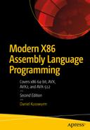
Raw data signal (top plot) and its smoothed counterpart (bottom plot)
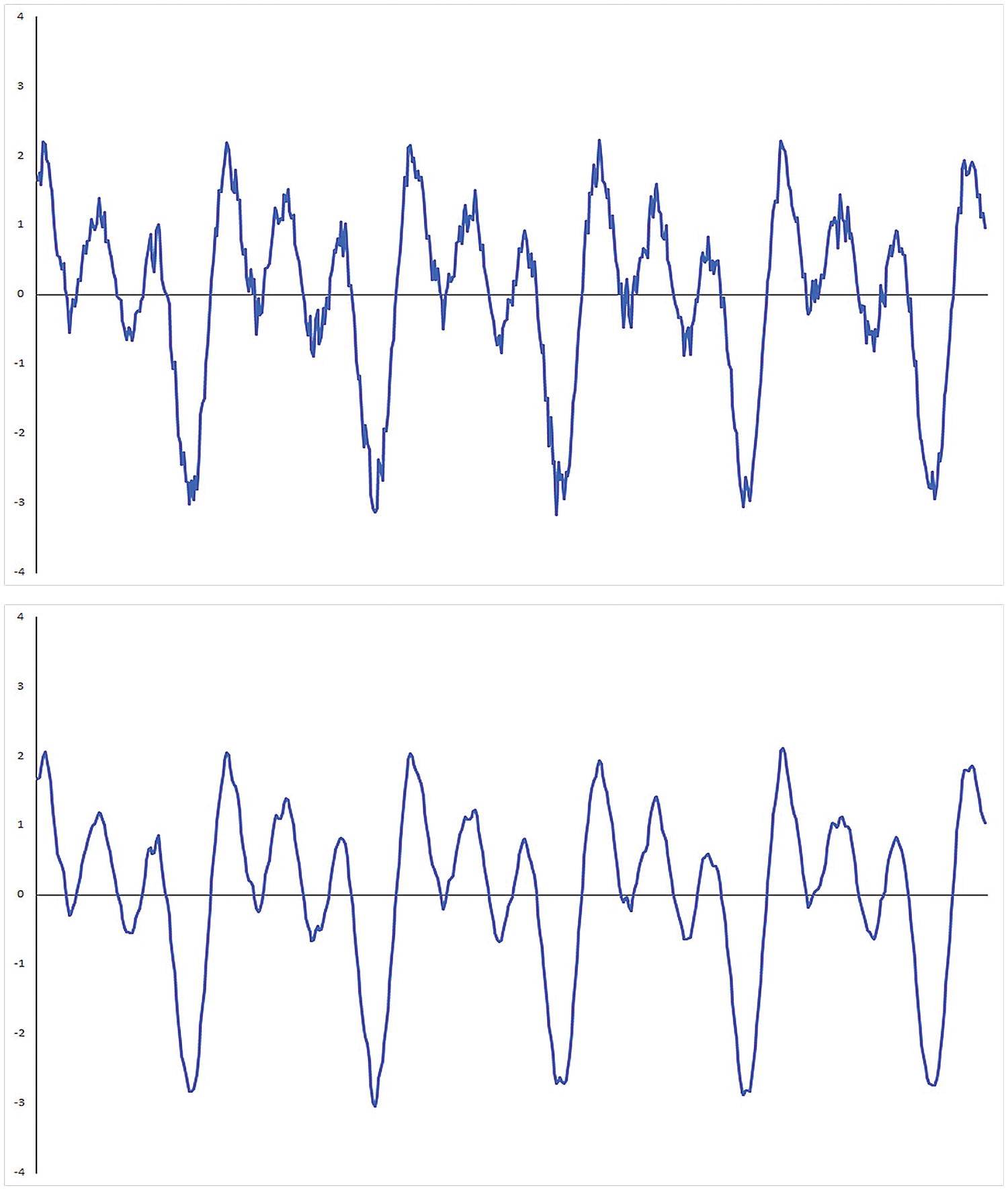
Application of a smoothing operator with an input signal element
The purpose of the preceding overview was to provide just enough background math to understand the source code examples. Numerous tomes have been published that explain convolution and signal processing theory in significantly greater detail. Appendix A contains a list of introductory references that you can consult for additional information about convolution and signal processing theory.
Scalar FMA
Example Ch11_01
The C++ code in Listing 11-1 begins with the header file Ch11_01.h, which contains the requisite function declarations for this example. The source code for function CreateSignal is next. This function constructs a synthetic input signal for test purposes. The synthetic input signal consists of three separate sinusoidal waveforms that are summed. Each waveform includes a small amount of random noise. The input signal generated by CreateSignal is the same signal that’s shown in the top plot of Figure 11-1.
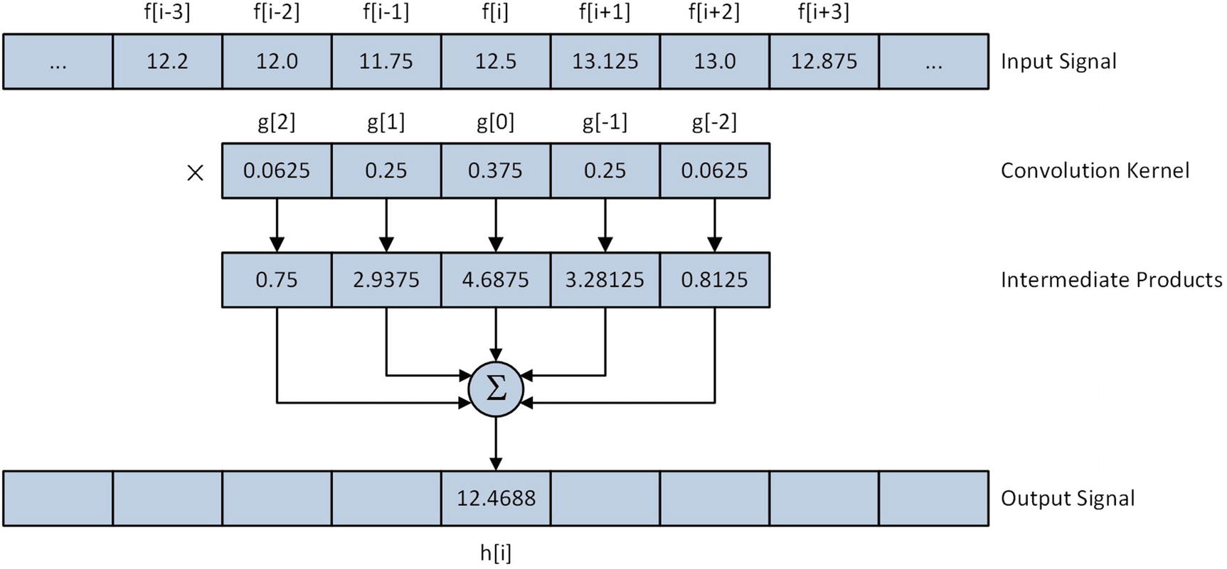
Padded input signal array following execution of PadSignal using a five-element convolution kernel
The C++ function Convolve1 contains code that exercises several different implementations of the discrete convolution algorithm. Near the top of this function is a single-precision floating-point array named kernel, which contains the convolution kernel coefficients. The coefficients in kernel represent a discrete approximation of a Gaussian (or low pass) filter. When convolved with an input signal array, these coefficients reduce the amount of noise that’s present in a signal, as shown in the bottom plot of Figure 11-1. The padded input signal array x2 is created next using the previously described functions CreateSignal and PadSignal. Note that the C++ template class unique_ptr<> is used to manage storage space for both x2 and the unpadded array x1.
Following the generation of the input signal array x2, Convolve1 allocates storage space for four output signal arrays. The functions that implement different variations of the convolution algorithms are then called. The first two functions, Convolve1Cpp and Convolve1_, contain C++ and assembly language code that carry out their convolutions using the nested for loop technique described earlier in this section. The functions Convolve1Ks5Cpp and Convolve1Ks5_ are optimized for convolution kernels containing five elements. Real-world signal processing software regularly employs convolution functions that are optimized for specific kernel sizes since they’re often significantly faster, as you will soon see.
The function Convolve1Cpp begins its execution by validating argument values kernel_size and num_pts. The next statement, x += ks2, adjusts the input signal array pointer so that it points to the first true input signal array element. Recall that the input signal array x is padded with extra values to ensure correct processing when the convolution kernel is superimposed over the first two and last two input signal elements. Following the pointer x adjustment is the actual code that performs the convolution. The nested for loops implement the discrete convolution equation that was described earlier in this section. Note that the index value used for kernel is offset by ks2 to account for the negative indices of the inner loop. Following function Convolve1Cpp is the function Convolve1Ks5Cpp, which uses explicit C++ statements to calculate convolution sum-of-products instead of a for loop.
The functions Convolve1_ and Convolve1Ks5_ are the assembly language counterparts of Convolve1Cpp and Convolve1Ks5Cpp, respectively. After its prolog, Convolve1_ validates argument values kernel_size and num_pts. This is followed by an initialization code block that begins by loading num_pts into R8. The ensuing shr r10d,1 instruction loads ks2 into register R10D. The final initialization code block instruction, lea rdx,[rdx+r10*4], loads register RDX with the address of the first input signal array element in x.
Similar to the C++ code, Convole1_ uses two nested for loops to perform the convolution. The outer loop, which is labeled LP1, starts with a vxorps xmm5,xmm5,xmm5 instruction that sets sum equal to 0.0. The ensuing mov r11,r10 and neg r11 instructions set inner loop index counter k (R11) to -ks2. The label LP2 marks the start of the inner loop. The mov rbx,rax and sub rbx,r11 instructions calculate the index, or i – k, of the next element in x. This is followed by a vmovss xmm0,real4 ptr [rdx+rbx*4] instruction that loads x[i - k] into XMM0. Next, the mov rsi,r11 and add rsi,r10 instructions calculate k + ks2. The subsequent vfmadd231ss xmm5,xmm0,[r9+rsi*4] instruction calculates sum += x[i - k] * kernel[k + ks2]. As discussed in Chapter 8, the FMA instruction vfmadd231ss carries out its operations using a single rounding operation. Depending on the algorithm, the use of a vfmadd231ss instruction instead of an equivalent sequence of vmulss and vaddss instructions may result in slightly faster execution times.
Following the execution of the vfmadd231ss instruction, the add r11,1 instruction computes k++ and the inner loop repeats until k > ks2 is true. Subsequent to the completion of the inner loop, the vmovss real4 ptr [rcx+rax*4],xmm5 instruction saves the current sum-of-products result to y[i]. The add rax,1 instruction updates index counter i, and the outer loop LP1 repeats until all of the input signal data points have been processed.
Mean Execution Times (Microseconds) for Convolution Functions Using Five-Element Convolution Kernel (2,000,000 Signal Points)
CPU | Convolve1Cpp | Convolve1_ | Convolve1Ks5Cpp | Convolve1Ks5_ |
|---|---|---|---|---|
i7-4790S | 6148 | 6844 | 2926 | 2841 |
i9-7900X | 5607 | 6072 | 2808 | 2587 |
i7-8700K | 5149 | 5576 | 2539 | 2394 |
Packed FMA
Example Ch11_02
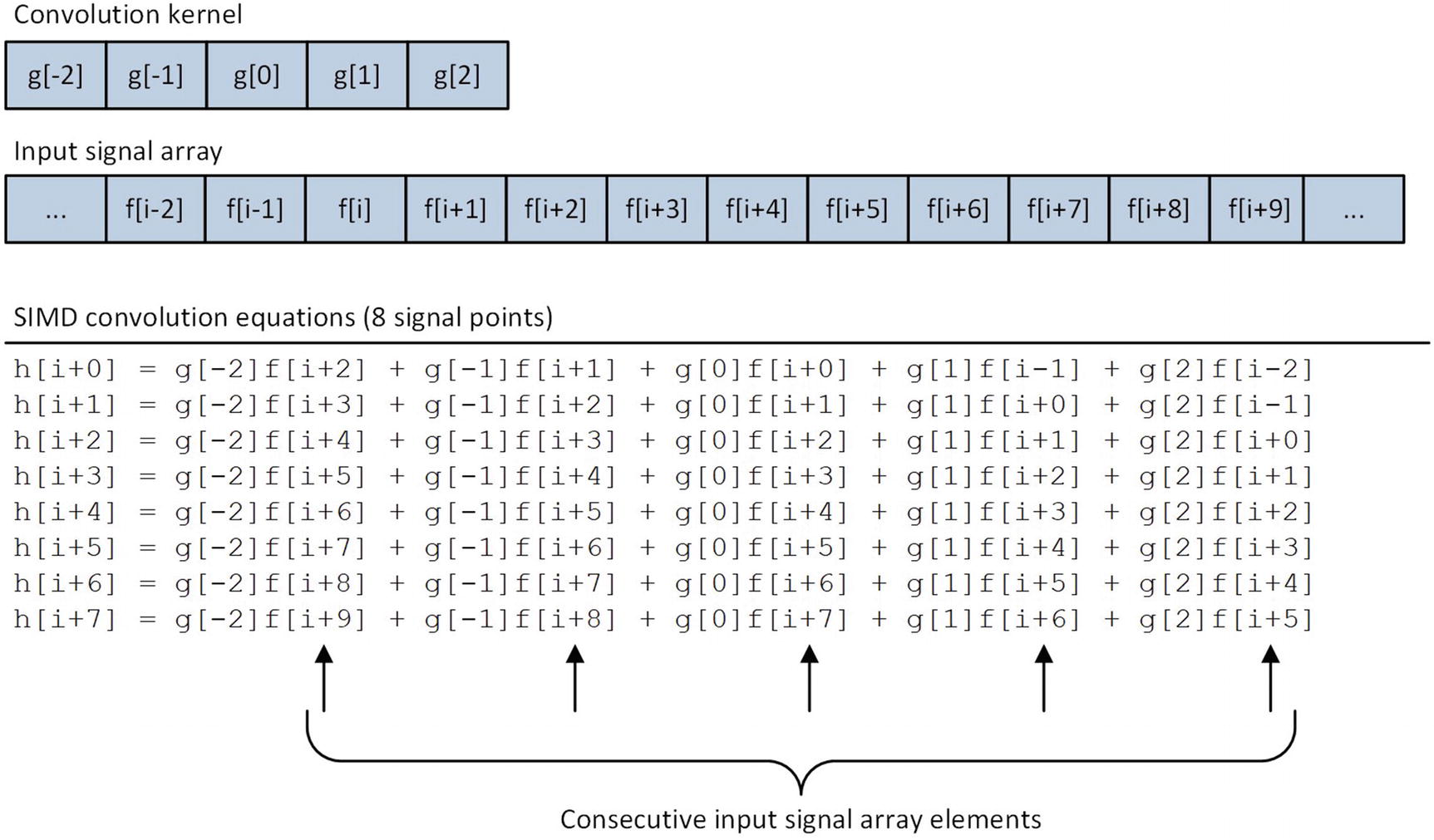
SIMD convolution equations for five-element convolution kernel
The C++ function Convolve2 is located near the top of Listing 11-2. This function creates and initializes the padded input signal array x2 using the same CreateSignal and PadSignal functions that were employed in example Ch11_01. It also uses the C++ template class AlignedArray to allocate storage for the output signal arrays y5 and y6. In this example, the output signal arrays must be properly aligned since the assembly language functions use the vmovaps instruction to save calculated results. Proper alignment of the input signal arrays x1 and x2 is optional and used here for consistency. Following the allocation of the signal arrays, Convolve2 invokes the assembly language functions Convolve2_ and ConvolveKs5_; it then saves the output signal array data to a CSV file.
The function Convolve2_ begins its execution by validating argument values kernel_size and num_pts. It also verifies that output signal array y is properly aligned. The convolution code block of Convolve2_ employs the same nested for loop construct that was used in example Ch11_01. Each outer loop LP1 iteration begins with a vxorps ymm0,ymm0,ymm0 instruction that initializes eight single-precision floating-point sum values to 0.0. The ensuing mov r11,r10 and neg r11 instructions initialize k with the value -ks2. The inner loop starts by calculating and saving i - k in register RAX. The subsequent vmovups ymm1,ymmword ptr [rdx+rax*4] instruction loads input signal array elements x[i - k]:x[i - k + 7] into register YMM1. This is followed by a vbroadcastss ymm2,real4 ptr [r9+rax*4] instruction that broadcasts kernel[k + ks2] to each single-precision floating-point element position in YMM2. The vfmadd231ps ymm0,ymm1,ymm2 instruction multiplies each input signal array element in YMM1 by kernel[k + ks2] and adds this intermediate result to the packed sums in register YMM0. The inner loop repeats until k > ks2 is true. Following the completion of the inner loop, the vmovaps ymmword ptr [rcx+rbx*4],ymm0 instruction saves the eight convolution results to output signal array elements y[i]:y[i + 7]. Outer loop index counter i is then updated and the loop repeats until all input signal elements have been processed.
The assembly language function Convolve2Ks5_ is optimized for five-element convolution kernels. Following the requisite argument validations, a series of vbroadcastss instructions load kernel coefficients kernel[0]–kernel[4] into registers YMM4–YMM8, respectively. The two vxorps instructions located at the top of the processing loop initialize the intermediate packed sums to 0.0. The array index j = i + ks2 is then calculated and saved in register R11. The ensuing vmovups ymm0,ymmword ptr [rdx+r11*4] instruction loads input signal array elements x[j]:x[j + 7] into register YMM0. This is followed by a vfmadd231ps ymm2,ymm0,ymm4 instruction that multiplies each input signal array element in YMM0 by kernel[0]; it then adds these values to the intermediate packed sums in YMM2. Convolve2Ks5_ then uses four additional sets of vmovups and vfmadd231ps instructions to compute results using coefficients kernel[1]–kernel[4]. Similar to the function Convolve1Ks5_ in source code example Ch11_01, Convolve2Ks5_ also uses two YMM registers for its intermediate FMA sums, which facilitates simultaneous execution of two vfmadd231ps instructions on processors with dual 256-bit wide FMA execution units. Following the FMA operations, a vmovaps ymmword ptr [rcx+rax*4],ymm0 instruction saves the eight output signal array elements to y[i]:y[i + 7].
Mean Execution Times (Microseconds) for SIMD Convolution Functions Using Five-Element Convolution Kernel (2,000,000 Signal Points)
CPU | Convolve2_ | Convolve2Ks5_ | Convolve2Ks5Test_ |
|---|---|---|---|
i7-4790S | 1244 | 1067 | 1074 |
i9-7900X | 956 | 719 | 709 |
i7-8700K | 859 | 595 | 597 |
Examples of Value Discrepancies Using FMA and Non-FMA Instruction Sequences
Index | x[] | Convolve2Ks5_ | Convolve2Ks5Test_ |
|---|---|---|---|
33 | 1.3856432 | 1.1940877 | 1.1940879 |
108 | 1.3655651 | 1.4466031 | 1.4466029 |
180 | -2.8778596 | -2.7348523 | -2.7348526 |
277 | -1.7654022 | -2.0587211 | -2.0587208 |
403 | 2.0683382 | 2.0299273 | 2.0299270 |
General-Purpose Register Instructions
As mentioned and discussed in Chapter 8, several general-purpose register instructions set extensions have been added to the x86 platform in recent years (see Tables 8-2 and 8-5). In this section, you learn how to use some of these instructions. The first source code example illustrates how to use the flagless multiplication and shift instructions. A flagless instruction executes its operation without modifying any of the status flags in RFLAGS, which can be faster than an equivalent flag-based instruction depending on the specific use case. The second source code example demonstrates several advanced bit-manipulation instructions. The source code examples of this section require a processor that supports the BMI1 , BMI2 , and LZCNT instruction set extensions.
Flagless Multiplication and Shifts
Example Ch11_03
The C++ code for example Ch11_03 contains two functions named GprMulx and GprShiftx. These functions initialize test cases that demonstrate flagless multiplication and shift operations, respectively. Note that both GprMulx and GprShiftx define an array of type uint64_t named flags. This array is used to show the contents of the status flags in RFLAGS before and after the execution of each flagless instruction. The remaining code in both GprMulx and GprShiftx format and stream results to cout.
The assembly language function GprMulx begins its execution by saving a copy of RFLAGS. The ensuing mulx r11d,r10d,ecx instruction performs a 32-bit unsigned integer multiplication using implicit source operand EDX (argument value b) with explicit source operand ECX (argument value a). The 64-bit product is then saved in register pair R11D:R10D. Following the execution of the mulx instruction, the contents of RFLAGS are saved again for comparison purposes. The mulx instruction also supports flagless multiplications using 64-bit operands. When used with 64-bit operands, register RDX is employed as the implicit operand and two 64-bit general-purpose registers must be used for the destination operands.
Enhanced Bit Manipulation
Example Ch11_04
The C++ code in Listing 11-4 contains three short functions that set up test cases for the assembly language functions. The first function, GprCountZeroBits, initializes a test array that’s used to demonstrate the lzcnt (Count the Number of Leading Zero Bits ) and tzcnt (Count the Number of Trailing Zero Bits ) instructions. The second function, GprExtractBitField, prepares test data for the bextr (Bit Field Extract) instruction. The final C++ function in Listing 11-4 is named GprAndNot. This function loads test arrays with data that’s used to illuminate execution of the andn (Bitwise AND NOT) instruction.
The BMI1 and BMI2 instruction set extensions also include other enhanced bit-manipulation instructions that can be used to implement specific algorithms or carry out specialized operations. These instructions are listed in Table 8-5.
Half-Precision Floating-Point Conversions
Example Ch11_05
The C++ function main starts its execution by loading single-precision floating-point test values into array x. It then exercises the half-precision floating-point conversion functions SingleToHalfPrecision_ and HalfToSinglePrecision_. Note that the function SingleToHalfPrecision_ requires a third argument, which specifies the rounding mode to use when converting floating-point values from single-precision to half-precision. Also note that an array type of uint16_t is used to store the half-precision floating-point results since C++ does not natively support a half-precision floating-point data type.
Rounding Mode Options for the vcvtps2ph Instruction
Immediate Operand Bits | Value | Description |
|---|---|---|
1:0 | 00b | Round to nearest |
01b | Round down (toward -∞) | |
10b | Round up (toward +∞) | |
11b | Round toward zero (truncate) | |
2 | 0 | Use rounding mode specified in immediate operand bits 1:0 |
1 | Use rounding mode specified in MXCSR.RC | |
7:3 | Ignored | Not used |
Summary
FMA instructions are often employed to implement numerically-oriented algorithms such as discrete convolutions, which are used extensively in a wide variety of problem domains, including signal processing and image processing.
Assembly language functions that employ sequences of consecutive FMA instructions should use multiple XMM or YMM registers to store intermediate sum products. Using multiple registers helps avoid data dependencies that can preclude the processor from executing multiple FMA instructions simultaneously.
Value discrepancies normally occur between functions that implement the exact same algorithm or operation using FMA and non-FMA instruction sequences. The significance of these discrepancies depends on the application.
Assembly language functions can use the mulx, sarx, shlx, and shrx instructions to carry out flagless unsigned integer multiplication and shifts. These instructions may yield slightly faster performance than their flag-based counterparts in algorithms that perform consecutive multiplication and shift operations.
Assembly language functions can use the lzcnt, tzcnt, bextr, and andn instructions to perform advanced bit-manipulation operations.
Assembly language functions can use the vcvtps2ph and vcvtph2ps instructions to perform conversions between single-precision and half-precision floating-point values.