Artificial Neural Network (ANN )

Before jumping into details of deep learning , I think it is very important to briefly understand how human vision works. The human brain is a complex connected neural network where different regions of the brain are responsible for different jobs, and these regions are machines of the brain that receive signals and processes it to take necessary action. Figure 6-1 shows the visual pathway of the human brain.

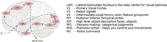
Figure 6-1. Visual pathway

Our brain is made up of a cluster of small connected units called neurons, which send electrical signals to one another. The long-term knowledge is represented by the strength of the connections between neurons. When we see objects, light travels through the retina and the visual information gets converted to electrical signals, and further on the electric signal passes through the hierarchy of connected neurons of different regions within the brain in a few milliseconds to decode signals/information.

What Goes Behind, When Computers Look at an Image?

In computers an image is represented as one large three-dimensional array of numbers. For example, consider Figure 6-2; it is the handwritten digit image of gray scale 28x28x1 (width x height x depth) size resulting in 784 data points. Each number in the array is an integer that ranges from 0 (black) to 255(white). In a typical classification problem the model has to turn this large matrix into a single label. For a color image additionally it will have three color channels: Red, Green, Blue (RGB) for each pixel, so the same image in color would be of size 28x28x3 = 2352 data points.

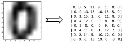
Figure 6-2. Handwritten digit(zero)image and correponding array

Why Not a Simple Classification Model for Images?

Image classification can be challenging for a computer as there are a variety of challenges associated with representation of the images. A simple classification model might not be able to address most of these issues without a lot of feature engineering effort. Let’s understand some of the key issues (refer to Table 6-2).

Table 6-2. Visual challenges in image data

Description	Example
View point variation : Same object can have different orientation.
Scale and illumination variation: Variation in object’s size and the level of illumination on pixel level can vary.
Deformation/twist and intra-class variation: Non-rigid bodies can be deformed in great ways and there can be different types of objects with varying appearance within a class.
Blockage: Only small portion of object in interest can be visible.
Background clutter : Objects can blend into their environment, which will make it hard to identify.

Perceptron – Single Artificial Neuron

Inspired by the biological neurons, McCulloch and Pitts in 1943 introduced the concept of perceptron as an artificial neuron that is the basic building block of the artificial neural network. They are not only named after their biological counterparts but also modeled after the behavior of the neurons in our brain. See Figure 6-3.

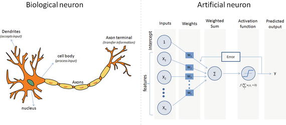
Figure 6-3. Biological vs. Artificial Neuron

Biological neurons have dendrites to receive signals, a cell body to process them, and an axon/axon terminal to transfer signals out to other neurons. Similarly an artificial neuron has multiple input channels to accept training samples represented as a vector, and a processing stage where the weights(w) are adjusted such that the output error (actual vs. predicted) is minimized. Then the result is fed into an activation function to produce output, for example, a classification label. The activation function for a classification problem is a threshold cutoff (standard is .5) above which class is 1 else 0. Let’s see how this can be implemented using scikit-learn. See Listing 6-1.

Listing 6-1. Example code for sklearn perceptron

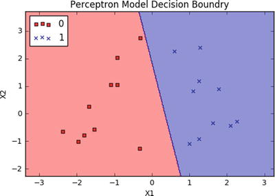
# import sklearn.linear_model.perceptron
from sklearn.linear_model import perceptron
import matplotlib.pyplot as plt
from matplotlib.colors import ListedColormap

# Let's use sklearn make_classification function to create some test data.
from sklearn.datasets import make_classification
X, y = make_classification(20, 2, 2, 0, weights=[.5, .5], random_state=2017)

# Create the model
clf = perceptron.Perceptron(n_iter=100, verbose=0, random_state=2017, fit_intercept=True, eta0=0.002)
clf.fit(X,y)

print "Prediction: " + str(clf.predict(X))
print "Actual:     " + str(y)
print "Accuracy:   " + str(clf.score(X, y)*100) + "%"

# Output the values
print "X1 Coefficient: " + str(clf.coef_[0,0])
print "X2 Coefficient: " + str(clf.coef_[0,1])
print "Intercept:      " + str(clf.intercept_)

# Plot the decision boundary using cusom function ‘plot_decision_regions’
plot_decision_regions(X, y, classifier=clf)
plt.title('Perceptron Model Decision Boundry')
plt.xlabel('X1')
plt.ylabel('X2')
plt.legend(loc='upper left')
plt.show()
#----output----
Prediction: [1 1 1 0 0 0 0 1 0 1 1 0 0 1 0 1 0 0 1 1]
Actual:     [1 1 1 0 0 0 0 1 0 1 1 0 0 1 0 1 0 0 1 1]
Accuracy:   100.0%
X1 Coefficient: 0.00575308754305
X2 Coefficient: 0.00107517941422
Intercept:      [-0.002]

Multilayer Perceptrons (Feedforward Neural Network)

To address the drawback of single perceptrons, multilayer perceptrons were proposed; also commonly known as a feedforward neural network, it is a composition of multiple perceptrons connected in different ways and operating on distinctive activation functions to enable improved learning mechanisms. The training sample propagates forward through the network and the output error is back propagated and the error is minimized using the gradient descent method, which will calculate a loss function for all the weights in the network. See Figure 6-4.

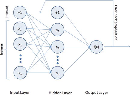
Figure 6-4. Multilayer perceptron representation

The activation function for a simple one-level hidden layer of a multilayer perceptron can be given by:

, where x _i is the input and W _ji ⁽¹⁾ is the input layer weights and W _kj ⁽²⁾ is the weight of hidden layer.

A multilayered neural network can have many hidden layers, where the network holds its internal abstract representation of the training sample. The upper layers will be building new abstractions on top of the previous layers. So having more hidden layers for a complex dataset will help the neural network to learn better.

As you can see from Figure 6-4, the MLP architecture has a minimum of three layers, that is, input, hidden, and output layers. The input layer’s neuron count will be equal to the total number of features and in some libraries an additional neuron for intercept/bias. These neurons are represented as nodes. The output layers will have a single neuron for regression models and binary classifier; otherwise it will be equal to the total number of class labels for multiclass classification models.

Note that using too few neurons for a complex dataset can result in an under-fitted model due to the fact that it might fail to learn the patterns in complex data. However, using too many neurons can result in an over-fitted model as it has capacity to capture patterns that might be noise or specific for the given training dataset. So to build an efficient multilayered neural network, the fundamental questions to be answered about hidden layers while implementation is 1) what is the ideal number of hidden layers?, and 2) what should be the number of neurons in hidden layers?

A widely accepted rule of thumb is that you can start with one hidden layer, as there is a theory that one hidden layer is sufficient for the majority of problems. Then, gradually increase the layers on a trial-and-error basis to see if there is any improvement in accuracy. The number of neurons in the hidden layer can ideally be the mean of the neurons in the input and output layers.

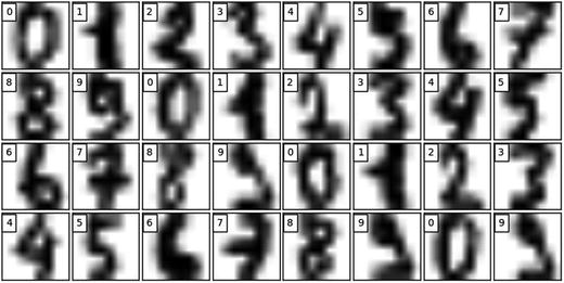
Let’s see an MLP algorithm in action from scikit-learn library on a classification problem. We’ll be using the digits dataset available as part of scikit-learn dataset, which is made up of 1797 samples (which is a subset of MNIST dataset) handwritten grayscale digit of 8x8 images.

Load MNIST Data

Listing 6-2. Example code for loading MNIST data for training MLP classifier

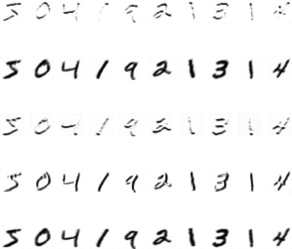
import pandas as pd
import numpy as np
import matplotlib.pyplot as plt

from sklearn.neural_network import MLPClassifier
from sklearn.model_selection import train_test_split
from sklearn.preprocessing import StandardScaler
from sklearn.metrics import confusion_matrix

from sklearn.datasets import load_digits
np.random.seed(seed=2017)

# load data
digits = load_digits()
print('We have %d samples'%len(digits.target))

## plot the first 32 samples to get a sense of the data
fig = plt.figure(figsize = (8,8))
fig.subplots_adjust(left=0, right=1, bottom=0, top=1, hspace=0.05, wspace=0.05)
for i in range(32):
    ax = fig.add_subplot(8, 8, i+1, xticks=[], yticks=[])
    ax.imshow(digits.images[i], cmap=plt.cm.gray_r)
ax.text(0, 1, str(digits.target[i]), bbox=dict(facecolor='white'))
#----output----
We have 1797 samples

Key Parameters for scikit-learn MLP

hidden_layer_sizes – You have to provide the number of hidden layers and neurons for each hidden layer. For example, hidden_layer_sizes – (5,3,3) means there are 3 hidden layers and the number of neurons for layer 1 is 5, layer 2 is 3, and for layer 3 is 3 respectively. The default value is (100,) that is, 1 hidden layer with 100 neurons.

Activation – This is the activation function for hidden layer, and there are four activation functions available for use, default is ‘relu’.

• relu: The rectified linear unit function, returns f(x) = max(0, x).

• logistic: The logistic sigmoid function, returns f(x) = 1 / (1 + exp(-x)).

• identity: No-op activation, useful to implement linear bottleneck, returns f(x) = x.

• tanh: The hyperbolic tan function, returns f(x) = tanh(x).

solver – This is for weight optimization’ there are three options available, the default being ‘adam’.

• adam: Stochastic gradient-based optimizer proposed by Kingma/Diederik/Jimmy Ba, which works well for large dataset.

• lbfgs: Belongs to family of quasi-Newton methods, works well for small datasets.

• sgd: Stochastic gradient descent.

max_iter – This is the maximum number of iterations for solver to converge, default is 200.

learning_rate_init – This is the initial learning rate to control step size for updating the weights (only applicable for solvers sgd/adam), default is 0.001.

It is recommended to scale or normalize your data before modeling as MLP is sensitive to feature scaling. See Listing 6-3.

Listing 6-3. Example code for sklearn MLP classifier

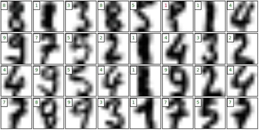
# split data to training and testing data
X_train, X_test, y_train, y_test = train_test_split(digits.data, digits.target, test_size=0.2, random_state=2017)
print 'Number of samples in training set: %d' %(len(y_train))
print 'Number of samples in test set: %d' %(len(y_test))

# Standardise data, and fit only to the training data
scaler = StandardScaler()
scaler.fit(X_train)

# Apply the transformations to the data
X_train_scaled = scaler.transform(X_train)
X_test_scaled = scaler.transform(X_test)

# Initialize ANN classifier
mlp = MLPClassifier(hidden_layer_sizes=(100), activation='logistic', max_iter = 100)

# Train the classifier with the traning data
mlp.fit(X_train_scaled,y_train)
#----output----
Number of samples in training set: 1437
Number of samples in test set: 360

MLPClassifier(activation='logistic', alpha=0.0001, batch_size='auto',
       beta_1=0.9, beta_2=0.999, early_stopping=False, epsilon=1e-08,
       hidden_layer_sizes=(30, 30, 30), learning_rate='constant',
       learning_rate_init=0.001, max_iter=100, momentum=0.9,
       nesterovs_momentum=True, power_t=0.5, random_state=None,
       shuffle=True, solver='adam', tol=0.0001, validation_fraction=0.1,
       verbose=False, warm_start=False)

print("Training set score: %f" % mlp.score(X_train_scaled, y_train))
print("Test set score: %f" % mlp.score(X_test_scaled, y_test))
#----output----
Training set score: 0.990953
Test set score: 0.983333

# predict results from the test data
X_test_predicted = mlp.predict(X_test_scaled)

fig = plt.figure(figsize=(8, 8))  # figure size in inches
fig.subplots_adjust(left=0, right=1, bottom=0, top=1, hspace=0.05, wspace=0.05)

# plot the digits: each image is 8x8 pixels
for i in range(32):
    ax = fig.add_subplot(8, 8, i + 1, xticks=[], yticks=[])
    ax.imshow(X_test.reshape(-1, 8, 8)[i], cmap=plt.cm.gray_r)

    # label the image with the target value
    if X_test_predicted[i] == y_test[i]:
        ax.text(0, 1, X_test_predicted[i], color='green', bbox=dict(facecolor='white'))
    else:
        ax.text(0, 1, X_test_predicted[i], color='red', bbox=dict(facecolor='white'))
#----output----

Restricted Boltzman Machines (RBM)

The RBM algorithm was proposed by Geoffrey Hinton (2007), which learns probability distribution over its sample training data inputs. It has seen wide applications in different areas of supervised/unsupervised machine learning such as feature learning, dimensionality reduction, classification, collaborative filtering, and topic modeling.

Consider the example movie rating discussed in the recommender system section. Movies like Avengers, Avatar, and Interstellar have strong associations with a latest fantasy and science fiction factor. Based on the user rating RBM will discover latent factors that can explain the activation of movie choices. In short, RBM describes variability among correlated variables of input dataset in terms of a potentially lower number of unobserved variables.

The energy function is given by E(v, h) = - a^Tv – b^Th – v^TWh

The probability function of a visible input layer can be given by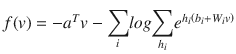

Let’s build a logistic regression model on a digits dataset with Bernoulli RBM and compare its accuracy with straight logistic regression (without Bernoulli RBM) model’s accuracy.

Let’s nudge the dataset set by moving the 8x8 images by 1 pixel on the left, right, down, and up to convolute the image. See Listing 6-4.

Listing 6-4. Function to nudge the dataset

# Function to nudge the dataset
def nudge_dataset(X, Y):
    """
    This produces a dataset 5 times bigger than the original one,
    by moving the 8x8 images in X around by 1px to left, right, down, up
    """
    direction_vectors = [
        [[0, 1, 0],
         [0, 0, 0],
         [0, 0, 0]],

        [[0, 0, 0],
         [1, 0, 0],
         [0, 0, 0]],

        [[0, 0, 0],
         [0, 0, 1],
         [0, 0, 0]],

        [[0, 0, 0],
         [0, 0, 0],
         [0, 1, 0]]]

    shift = lambda x, w: convolve(x.reshape((8, 8)), mode='constant',
                                 weights=w).ravel()
    X = np.concatenate([X] +
                       [np.apply_along_axis(shift, 1, X, vector)
        for vector in direction_vectors])
    Y = np.concatenate([Y for _ in range(5)], axis=0)
    return X, Y

The Bernoulli RBM assumes that the columns of our feature vectors fall within the range 0 to 1. However, the MNIST dataset is represented as unsigned 8-bit integers, falling within the range of 0 to 255.

Define a function to scale the columns into the range (0, 1). The scale function takes two parameters: our data matrix X and an epsilon value used to prevent division by zero errors. See Listing 6-5.

Listing 6-5. Example code for using Bernoulli RBM with classifier

# Example adapted from scikit-learn documentation
import numpy as np
import matplotlib.pyplot as plt
from sklearn import linear_model, datasets, metrics
from sklearn.model_selection import train_test_split
from sklearn.neural_network import BernoulliRBM
from sklearn.pipeline import Pipeline
from scipy.ndimage import convolve

# Load Data
digits = datasets.load_digits()
X = np.asarray(digits.data, 'float32')
y = digits.target

X, y = nudge_dataset(X, digits.target)

# Scale the features such that the values are between 0-1 scale
X = (X - np.min(X, 0)) / (np.max(X, 0) + 0.0001)

X_train, X_test, y_train, y_test = train_test_split(X, y, test_size=0.2, random_state=2017)
print X.shape
print y.shape
#----output----
(8985L, 64L)
(8985L,)

# Gridsearch for logistic regression
# perform a grid search on the 'C' parameter of Logistic
params = {"C": [1.0, 10.0, 100.0]}

Grid_Search = GridSearchCV(LogisticRegression(), params, n_jobs = -1, verbose = 1)
Grid_Search.fit(X_train, y_train)

# print diagnostic information to the user and grab the
print "Best Score: %0.3f" % (Grid_Search.best_score_)

# best model
bestParams = Grid_Search.best_estimator_.get_params()

print bestParams.items()
#----output----
Fitting 3 folds for each of 3 candidates, totalling 9 fits
Best Score: 0.774
[('warm_start', False), ('C', 100.0), ('n_jobs', 1), ('verbose', 0), ('intercept_scaling', 1), ('fit_intercept', True), ('max_iter', 100), ('penalty', 'l2'), ('multi_class', 'ovr'), ('random_state', None), ('dual', False), ('tol', 0.0001), ('solver', 'liblinear'), ('class_weight', None)]
# evaluate using Logistic Regression and only the raw pixel
logistic = LogisticRegression(C = 100)
logistic.fit(X_train, y_train)

print "Train accuracy: ", metrics.accuracy_score(y_train, logistic.predict(X_train))
print "Test accuracyL ", metrics.accuracy_score(y_test, logistic.predict(X_test))
#----output----
Train accuracy:  0.797440178075
Test accuracyL  0.800779076238

Let’s perform a grid search for RBM + Logistic Regression model. A grid search is on the learning rate, number of iterations, and number of components on the RBM and C for Logistic Regression. See Listing 6-6.

Listing 6-6. Example code for grid search with RBM + logistic regression

# initialize the RBM + Logistic Regression pipeline
rbm = BernoulliRBM()
logistic = LogisticRegression()
classifier = Pipeline([("rbm", rbm), ("logistic", logistic)])

params = {
    "rbm__learning_rate": [0.1, 0.01, 0.001],
    "rbm__n_iter": [20, 40, 80],
    "rbm__n_components": [50, 100, 200],
    "logistic__C": [1.0, 10.0, 100.0]}

# perform a grid search over the parameter
Grid_Search = GridSearchCV(classifier, params, n_jobs = -1, verbose = 1)
Grid_Search.fit(X_train, y_train)

# print diagnostic information to the user and grab the
# best model
print "Best Score: %0.3f" % (Grid_Search.best_score_)

print "RBM + Logistic Regression parameters"
bestParams = Grid_Search.best_estimator_.get_params()

# loop over the parameters and print each of them out
# so they can be manually set
for p in sorted(params.keys()):
    print "\t %s: %f" % (p, bestParams[p])
#----output----
Fitting 3 folds for each of 81 candidates, totalling 243 fits
Best Score: 0.505
RBM + Logistic Regression parameters
         logistic__C: 100.000000
         rbm__learning_rate: 0.001000
         rbm__n_components: 200.000000
         rbm__n_iter: 20.000000

# initialize the RBM + Logistic Regression classifier with
# the cross-validated parameters
rbm = BernoulliRBM(n_components = 200, n_iter = 20, learning_rate = 0.1, verbose = False)
logistic = LogisticRegression(C = 100)

# train the classifier and show an evaluation report
classifier = Pipeline([("rbm", rbm), ("logistic", logistic)])
classifier.fit(X_train, y_train)

print metrics.accuracy_score(y_train, classifier.predict(X_train))
print metrics.accuracy_score(y_test, classifier.predict(X_test))
#----output----
0.936839176405
0.932109070673

# plot RBM components
plt.figure(figsize=(15, 15))
for i, comp in enumerate(rbm.components_):
    plt.subplot(20, 20, i + 1)
    plt.imshow(comp.reshape((8, 8)), cmap=plt.cm.gray_r,
       interpolation='nearest')
    plt.xticks(())
    plt.yticks(())
plt.suptitle('200 components extracted by RBM', fontsize=16)
plt.show()
#----output----

Notice that the logistic regression model with RBM lifts the model score by more than 10% compared to the model without RBM.

Stacked RBM is known as Deep Believe Network (DBN), which is an initialization technique. However, this technique was popular during 2006-2007, and is reasonably outdated. So there is no out-of-box implementation of DBN in Keras. However if you are interested in a simple DBN implementation, I recommend you to have a look at https://github.com/albertbup/deep-belief-network , which has an MIT license.

MLP Using Keras

In Keras, neural networks are defined as a sequence of layers, and the container for these layers is the sequential class. The sequential models are linear stack of layers, and each layer is an object that feeds into the next.

The first layer in the neural network will define the number of inputs to expect. The activation functions that transform a summed signal from each neuron in a layer, the same can be extracted and added to the sequential as a layer-like object called activation. The choice of action depends on the type of problem (like regression or binary classification or multiclass classification) that we are trying to address. See Listing 6-7.

Listing 6-7. Example code for Keras MLP

from matplotlib import pyplot as plt
import numpy as np
np.random.seed(2017)

from keras.models import Sequential
from keras.datasets import mnist
from keras.layers import Dense, Activation, Dropout, Input
from keras.models import Model
from keras.utils import np_utils

# from keras.utils.visualize_util import plot
from IPython.display import SVG
from keras import backend as K
from keras.callbacks import EarlyStopping
from keras.utils.visualize_util import model_to_dot, plot

# load data
(X_train, y_train), (X_test, y_test) = mnist.load_data()

X_train = X_train.reshape(X_train.shape[0], input_unit_size)
X_test  = X_test.reshape(X_test.shape[0], input_unit_size)
X_train = X_train.astype('float32')
X_test  = X_test.astype('float32')

# Scale the values by dividing 255 i.e., means foreground (black)
X_train /= 255
X_test  /= 255

# one-hot representation, required for multiclass problems
y_train = np_utils.to_categorical(y_train, nb_classes)
y_test = np_utils.to_categorical(y_test, nb_classes)

print('X_train shape:', X_train.shape)
print(X_train.shape[0], 'train samples')
print(X_test.shape[0], 'test samples')
#----output----
('X_train shape:', (60000, 784))
(60000, 'train samples')
(10000, 'test samples')

nb_classes = 10 # class size
# flatten 28*28 images to a 784 vector for each image
input_unit_size = 28*28

# create model
model = Sequential()
model.add(Dense(input_unit_size, input_dim=input_unit_size, init='normal', activation='relu'))
model.add(Dense(nb_classes, init='normal', activation='softmax'))

Compilation is a model that is a pre-compute step that transforms the sequence of layers that we defined into a highly efficient series of matrix transforms. It takes three arguments: an optimizer, a loss function, and a list of evaluation metrics.

Unlike scikit-learn implementation, Keras provides a rich number of optimizers such as SGD (Stochastic gradient descent), RMSprop, Adagrad (Adaptive subgradient), Adadelta (adaptive learning rate), Adam, Adamax, Nadam, and TFOptimizer. For brevity, I won’t explain these here but recommend that you refer to the official Keras site for further reference.

Some standard loss functions are ‘mse’ for regression, binary_crossentropy (logarithmic loss) for binary classification, and categorical_crossentropy (multiclass logarithmic loss) for multiclassification problems.

The standard evaluation metrics for different types of problems are supported and you can pass a list for them to evaluate. See Listing 6-8.

Listing 6-8. Compile model

# Compile model
model.compile(loss='categorical_crossentropy', optimizer='adam', metrics=['accuracy'])

The network is trained using a back propogation algorithm, and optimized according to the specified method, loss function. Each epoch can be partitioned into batches. See Listing 6-9.

Listing 6-9. Train model and evaluate

# model training
model.fit(X_train, y_train, validation_data=(X_test, y_test), nb_epoch=5, batch_size=500, verbose=2)

# Final evaluation of the model
scores = model.evaluate(X_test, y_test, verbose=0)
print("Error: %.2f%%" % (100-scores[1]*100))
#----output----
Train on 60000 samples, validate on 10000 samples
Epoch 1/5
6s - loss: 0.3828 - acc: 0.8922 - val_loss: 0.1866 - val_acc: 0.9486
Epoch 2/5
6s - loss: 0.1561 - acc: 0.9559 - val_loss: 0.1274 - val_acc: 0.9630
Epoch 3/5
5s - loss: 0.1077 - acc: 0.9697 - val_loss: 0.0991 - val_acc: 0.9704
Epoch 4/5
6s - loss: 0.0803 - acc: 0.9777 - val_loss: 0.0842 - val_acc: 0.9747
Epoch 5/5
6s - loss: 0.0616 - acc: 0.9829 - val_loss: 0.0771 - val_acc: 0.9754
Error: 2.46%

Autoencoders

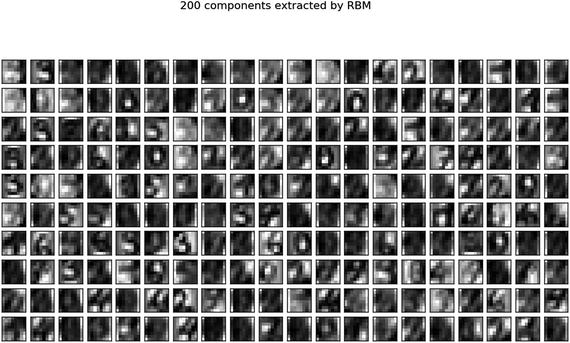
As the name suggests, an autoencoder aims to learn encoding as a representation of training sample data automatically without human intervention. The autoencoder is widely used for dimensionality reduction and data de-nosing. See Figure 6-5.

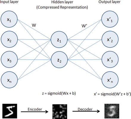
Figure 6-5. Autoencoder

Building an autoencoder will typically have three elements .

1. Encoding function to map input to a hidden representation through a nonlinear function, z = sigmoid (Wx + b).

2. A decoding function such as x’ = sigmoid(W’y + b’), which will map back into reconstruction x’ with same shape as x.

3. A loss function, which is a distance function to measure the information loss between the compressed representation of data and the decompressed representation. Reconstruction error can be measured using traditional squared error ||x-z||².

We’ll be using the well-known MNIST database of handwritten digits, which consists of approximately 70,000 total samples of handwritten grayscale digit images for numbers 0 to 9, each image of size is 28x28 and intensity level varies from 0 to 255 with accompanying label integer 0 to 9 for 60,000 of them and remaining ones without labels (test dataset).

Dimension Reduction Using Autoencoder

Listing 6-10. Example code for dimension reduction using autoencoder

import numpy as np
np.random.seed(2017)

from keras.datasets import mnist
from keras.models import Model
from keras.layers import Input, Dense
from keras.optimizers import Adadelta
from keras.utils import np_utils

# from keras.utils.visualize_util import plot
from IPython.display import SVG
from keras import backend as K
from keras.callbacks import EarlyStopping
from keras.utils.visualize_util import model_to_dot
from matplotlib import pyplot as plt

# Load mnist data
input_unit_size = 28*28
(X_train, y_train), (X_test, y_test) = mnist.load_data()

# function to plot digits
def draw_digit(data, row, col, n):
    size = int(np.sqrt(data.shape[0]))
    plt.subplot(row, col, n)
    plt.imshow(data.reshape(size, size))
    plt.gray()

# Normalize
X_train = X_train.reshape(X_train.shape[0], input_unit_size)
X_train = X_train.astype('float32')
X_train /= 255
print('X_train shape:', X_train.shape)
#----output----
('X_train shape:', (60000, 784))

# Autoencoder
inputs = Input(shape=(input_unit_size,))
x = Dense(144, activation='relu')(inputs)
outputs = Dense(input_unit_size)(x)
model = Model(input=inputs, output=outputs)
model.compile(loss='mse', optimizer='adadelta')

SVG(model_to_dot(model, show_shapes=True).create(prog='dot', format='svg'))
#----output----

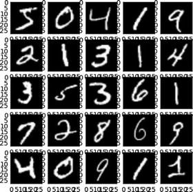
Note that the 784 dimension is reduced through encoding to 144 in the hidden layer and again in layer 3 constructed back to 784 using decoder.
model.fit(X_train, X_train, nb_epoch=5, batch_size=258)
#----output----
Epoch 1/5
60000/60000 [==============================] - 8s - loss: 0.0733
Epoch 2/5
60000/60000 [==============================] - 9s - loss: 0.0547
Epoch 3/5
60000/60000 [==============================] - 11s - loss: 0.0451
Epoch 4/5
60000/60000 [==============================] - 11s - loss: 0.0392
Epoch 5/5
60000/60000 [==============================] - 11s - loss: 0.0354

# plot the images from input layers
show_size = 5
total = 0
plt.figure(figsize=(5,5))
for i in range(show_size):
    for j in range(show_size):
        draw_digit(X_train[total], show_size, show_size, total+1)
        total+=1
plt.show()
#----output----

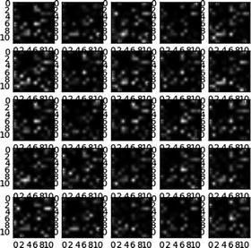
# plot the encoded (compressed) layer image
get_layer_output = K.function([model.layers[0].input],
                                 [model.layers[1].output])

hidden_outputs = get_layer_output([X_train[0:show_size**2]])[0]

total = 0
plt.figure(figsize=(5,5))
for i in range(show_size):
    for j in range(show_size):
        draw_digit(hidden_outputs[total], show_size, show_size, total+1)
        total+=1
plt.show()
#----output----

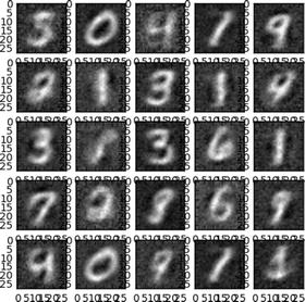
# Plot the decoded (de-compressed) layer images
get_layer_output = K.function([model.layers[0].input],
                                  [model.layers[2].output])

last_outputs = get_layer_output([X_train[0:show_size**2]])[0]

total = 0
plt.figure(figsize=(5,5))
for i in range(show_size):
    for j in range(show_size):
      draw_digit(last_outputs[total], show_size, show_size, total+1)
        total+=1
plt.show()
#----output----

De-noise Image Using Autoencoder

Discovering robust features from the compressed hidden layer is an important aspect to enable the autoencoder to efficiently reconstruct the input from a de-noised version or original image. This is addressed by the de-noising autoencoder, which is a stochastic version of autoencoder.

Let’s introduce some noise to the digit dataset and try to build a model to de-noise the image. See Listing 6-11.

Listing 6-11. Example code for de-noising using autoencoder

# Introducing noise to the image
noise_factor = 0.5
X_train_noisy = X_train + noise_factor * np.random.normal(loc=0.0, scale=1.0, size=X_train.shape)
X_train_noisy = np.clip(X_train_noisy, 0., 1.)

# Function for visualization
def draw(data, row, col, n):
    plt.subplot(row, col, n)
    plt.imshow(data, cmap=plt.cm.gray_r)
    plt.axis('off')

show_size = 10
plt.figure(figsize=(20,20))

for i in range(show_size):
    draw(X_train_noisy[i].reshape(28,28), 1, show_size, i+1)
plt.show()
#----output----

#Let’s fit a model on noisy training dataset.
model.fit(X_train_noisy, X_train, nb_epoch=5, batch_size=258)

# Prediction for denoised image
X_train_pred = model.predict(X_train_noisy)

show_size = 10
plt.figure(figsize=(20,20))

for i in range(show_size):
    draw(X_train_pred[i].reshape(28,28), 1, show_size, i+1)
plt.show()
#----output----

Note that we can tune the model to improve the sharpness of de-noised image.

Convolution Neural Network (CNN)

In the world of image classification, CNN has become the go-to algorithm to build efficient models. CNN’s are similar to ordinary neural networks, except that it explicitly assumes that the inputs are images, which allows us to encode certain properties into the architecture. These then make the forward function efficient to implement and reduces the parameters in the network. The neurons are arranged in three dimensions: width, height, and depth.

CNN on CIFAR10 Dataset

Let’s consider CIFAR-10 (Canadian Institute for Advanced Research), which is a standard computer vision and deep learning image dataset. It consists of 60,000 color photos of 32 by 32 pixel squared with RGB for each pixel, divided into 10 classes, which include common objects such as airplanes, automobiles, birds, cats, deer, dog, frog, horse, ship, and truck. Essentially each image is of size 32x32x3 (width x height x RGB color channels).

CNN consists of four main types of layers: input layer, convolution layer, pooling layer, fully connected layer.

The input layer will hold the raw pixel, so an image of CIFAR-10 will have 32x32x3 dimensions of input layer. The convolution layer will compute a dot product between the weights of small local regions from the input layer, so if we decide to have 5 filters the resulted reduced dimension will be 32x32x5. The RELU layer will apply an element-wise activation function that will not affect the dimension. The Pool layer will down sample the spatial dimension along width and height, resulting in dimension 16x16x5. Finally, the fully connected layer will compute the class score, and the resulted dimension will be a single vector 1x1x10 (10 class scores). Each neural in this layer is connected to all numbers in the previous volume. See Figure 6-6.

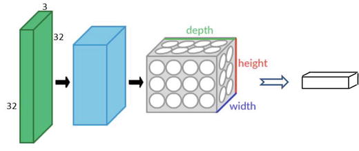
Figure 6-6. Convolution Neural Network

The next example illustration uses Keras with Theano aback end. To start Keras with Theano back end please run the following command while starting jupyter notebook, “KERAS_BACKEND=theano jupyter notebook.” See Listing 6-12 .

Listing 6-12. CNN using keras with theano backend on CIFAR10 dataset

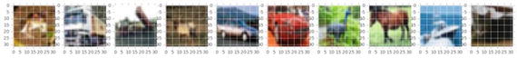
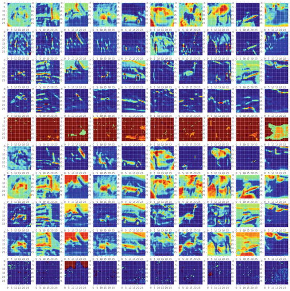
import keras
if K=='tensorflow':
    keras.backend.set_image_dim_ordering('tf')
else:
    keras.backend.set_image_dim_ordering('th')

from keras.models import Sequential
from keras.datasets import cifar10
from keras.layers import Dense, Activation, Flatten
from keras.optimizers import Adadelta
from keras.utils import np_utils
from keras.layers.convolutional import Convolution2D, MaxPooling2D
from keras.utils.visualize_util import model_to_dot, plot
from keras import backend as K
import numpy as np
from IPython.display import SVG

from matplotlib import pyplot as plt
import matplotlib.image as mpimg
%matplotlib inline

np.random.seed(2017)

batch_size = 256
nb_classes = 10
nb_epoch = 4
nb_filter = 10

img_rows, img_cols = 32, 32
img_channels = 3

# image dimension based on backend. 'th' = theano and 'tf' = tensorflow
if K.image_dim_ordering() == 'th':
    input_shape = (3, img_rows, img_cols)
else:
    input_shape = (img_rows, img_cols, 3)

(X_train, y_train), (X_test, y_test) = cifar10.load_data()
print('X_train shape:', X_train.shape)
print(X_train.shape[0], 'train samples')
print(X_test.shape[0], 'test samples')
X_train = X_train.astype('float32')
X_test = X_test.astype('float32')
X_train /= 255
X_test /= 255

Y_train = np_utils.to_categorical(y_train, nb_classes)
Y_test = np_utils.to_categorical(y_test, nb_classes)
#----output----
('X_train shape:', (50000, 3, 32, 32))
(50000, 'train samples')
(10000, 'test samples')

# Model Configuration
# define two groups of layers: feature (convolutions) and classification (dense)
feature_layers = [
    Convolution2D(nb_filters, nb_conv, nb_conv, input_shape=input_shape),
    Activation('relu'),
    Convolution2D(nb_filters, nb_conv, nb_conv),
    Activation('relu'),
    MaxPooling2D(pool_size=(nb_pool, nb_pool)),
    Flatten(),
]
classification_layers = [
    Dense(512),
    Activation('relu'),
    Dense(nb_classes),
    Activation('softmax')
]

# create complete model
model = Sequential(feature_layers + classification_layers)

model.compile(loss='categorical_crossentropy', optimizer="adadelta", metrics=['accuracy'])

# print model layer summary
print(model.summary())
#----output----
__________________________________________________________________________
Layer (type)                  Output Shape          Param #     Connected to
==========================================================================
convolution2d_1 (Convolution2D)  (None, 10, 30, 30) 280         convolution2d_input_1[0][0]
__________________________________________________________________________
activation_1 (Activation)        (None, 10, 30, 30) 0  convolution2d_1[0][0]
__________________________________________________________________________
convolution2d_2 (Convolution2D)  (None, 10, 28, 28) 910   activation_1[0][0]
__________________________________________________________________________
activation_2 (Activation)        (None, 10, 28, 28) 0  convolution2d_2[0][0]
__________________________________________________________________________
maxpooling2d_1 (MaxPooling2D)    (None, 10, 14, 14) 0     activation_2[0][0]
__________________________________________________________________________
flatten_1 (Flatten)              (None, 1960) 0         maxpooling2d_1[0][0]
__________________________________________________________________________
dense_1 (Dense)                  (None, 512) 1004032         flatten_1[0][0]
_________________________________________________________________________
activation_3 (Activation)        (None, 512) 0                 dense_1[0][0]
_______________________________________________________________________
dense_2 (Dense)                  (None, 10) 5130          activation_3[0][0]
__________________________________________________________________________
activation_4 (Activation)        (None, 10) 0                  dense_2[0][0]
=========================================================================
Total params: 1010352

# fit model
model.fit(X_train, Y_train, batch_size=batch_size, nb_epoch=nb_epoch, validation_data=(X_test, Y_test))
#----output----
Train on 50000 samples, validate on 10000 samples
Epoch 1/4
83s - loss: 1.9102 - acc: 0.3235 - val_loss: 1.5988 - val_acc: 0.4268
Epoch 2/4
90s - loss: 1.5174 - acc: 0.4671 - val_loss: 1.4651 - val_acc: 0.4846
Epoch 3/4
93s - loss: 1.3359 - acc: 0.5346 - val_loss: 1.4031 - val_acc: 0.5086
Epoch 4/4
85s - loss: 1.2222 - acc: 0.5739 - val_loss: 1.3008 - val_acc: 0.5483

Let’s visualize each layers. Note that we applied 10 filters.

# function for Visualization
def draw(data, row, col, n):
    plt.subplot(row, col, n)
    plt.imshow(data)

### Input layer (original image)
show_size = 10
plt.figure(figsize=(20,20))
for i in range(show_size):
    draw(X_train[i].reshape(3, 32, 32).transpose(1, 2, 0), 1, show_size, i+1)
plt.show()
#----output----

Notice below that in the hidden layers features are stored in 10 filters

# first layer
get_first_layer_output = K.function([model.layers[0].input], [model.layers[1].output])
first_layer = get_first_layer_output([X_train[0:show_size]])[0]

plt.figure(figsize=(20,20))

for img_index, filters in enumerate(first_layer, start=1):
    for filter_index, mat in enumerate(filters):
        pos = (filter_index)*show_size+img_index
        draw(mat, nb_filters, show_size, pos)
plt.show()
#----output----

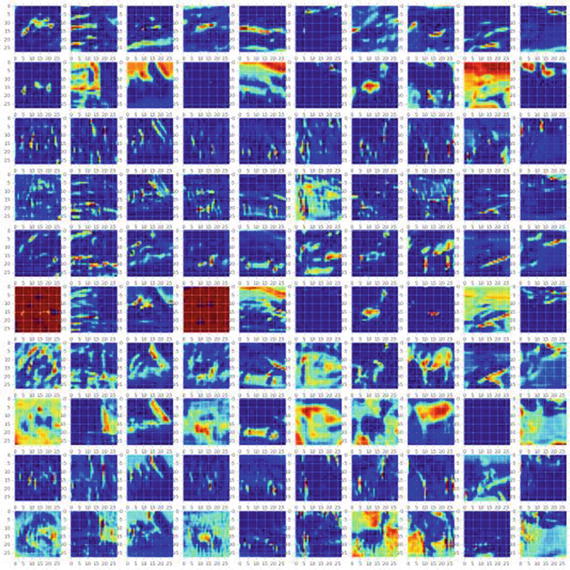
# second layer
get_second_layer_output = K.function([model.layers[0].input],
                          [model.layers[3].output])
second_layers = get_second_layer_output([X_train[0:show_size]])[0]

plt.figure(figsize=(20,20))

for img_index, filters in enumerate(second_layers, start=1):
    for filter_index, mat in enumerate(filters):
        pos = (filter_index)*show_size+img_index
        draw(mat, nb_filters, show_size, pos)
plt.show()
#----output----

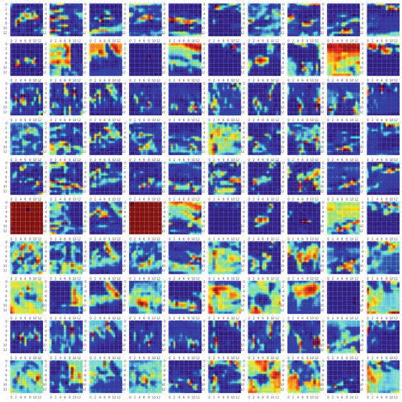
# third layer
get_third_layer_output = K.function([model.layers[0].input],
                  [model.layers[4].output])
third_layers = get_third_layer_output([X_train[0:show_size]])[0]

plt.figure(figsize=(20,20))

for img_index, filters in enumerate(third_layers, start=1):
    for filter_index, mat in enumerate(filters):
        pos = (filter_index)*show_size+img_index
        mat_size = mat.shape[1]
        draw(mat, nb_filters, show_size, pos)
plt.show()
#----output-----

CNN on MNIST Dataset

As an additional example, let’s look at how the CNN might look on a digits dataset. See Listing 6-13.

Listing 6-13. CNN using keras with theano back end on MNIST dataset

import keras
keras.backend.backend()
keras.backend.image_dim_ordering()

# using theano has backend
K = keras.backend.backend()
if K=='tensorflow':
    keras.backend.set_image_dim_ordering('tf')
else:
    keras.backend.set_image_dim_ordering('th')

from matplotlib import pyplot as plt
%matplotlib inline

import numpy as np
np.random.seed(2017)

from keras import backend as K
from keras.models import Sequential
from keras.datasets import mnist
from keras.layers import Dense, Dropout, Activation, Convolution2D, MaxPooling2D, Flatten
from keras.utils import np_utils
from keras.utils.visualize_util import plot
from keras.preprocessing import sequence

from keras import backend as K
from keras.utils.visualize_util import plot
from IPython.display import SVG, display
from keras.utils.visualize_util import model_to_dot, plot

img_rows, img_cols = 28, 28
nb_classes = 10

nb_filters = 5 # the number of filters
nb_pool = 2 # window size of pooling
nb_conv = 3 # window or kernel size of filter
nb_epoch = 5

# image dimension based on backend. ‘th’ = theano and ‘tf’ = tensorflow
if K.image_dim_ordering() == 'th':
    input_shape = (1, img_rows, img_cols)
else:
    input_shape = (img_rows, img_cols, 1)

# data
(X_train, y_train), (X_test, y_test) = mnist.load_data()

X_train = X_train.reshape(X_train.shape[0], 1, img_rows, img_cols)
X_test = X_test.reshape(X_test.shape[0], 1, img_rows, img_cols)
X_train = X_train.astype('float32')
X_test = X_test.astype('float32')
X_train /= 255
X_test /= 255
print('X_train shape:', X_train.shape)
print(X_train.shape[0], 'train samples')
print(X_test.shape[0], 'test samples')

# convert class vectors to binary class matrices
Y_train = np_utils.to_categorical(y_train, nb_classes)
Y_test = np_utils.to_categorical(y_test, nb_classes)
#----output----
('X_train shape:', (60000, 1, 28, 28))
(60000, 'train samples')
(10000, 'test samples')

# define two groups of layers: feature (convolutions) and classification (dense)
feature_layers = [
    Convolution2D(nb_filters, nb_conv, nb_conv, input_shape=input_shape),
    Activation('relu'),
    Convolution2D(nb_filters, nb_conv, nb_conv),
    Activation('relu'),
    MaxPooling2D(pool_size=(nb_pool, nb_pool)),
    Dropout(0.25),
    Flatten(),
]
classification_layers = [
    Dense(128),
    Activation('relu'),
    Dropout(0.5),
    Dense(nb_classes),
    Activation('softmax')
]

# create complete model
model = Sequential(feature_layers + classification_layers)

# define two groups of layers: feature (convolutions) and classification (dense)
feature_layers = [
    Convolution2D(nb_filters, nb_conv, nb_conv, input_shape=input_shape),
    Activation('relu'),
    Convolution2D(nb_filters, nb_conv, nb_conv),
    Activation('relu'),
    MaxPooling2D(pool_size=(nb_pool, nb_pool)),
    Dropout(0.25),
    Flatten(),
]
classification_layers = [
    Dense(128),
    Activation('relu'),
    Dropout(0.5),
    Dense(nb_classes),
    Activation('softmax')
]

# create complete model
model = Sequential(feature_layers + classification_layers)

print(model.summary())
#----output----
__________________________________________________________________________
Layer (type)                     Output ShapeParam #     Connected to
==========================================================================
convolution2d_1 (Convolution2D)  (None, 5, 26, 26) 50  
convolution2d_input_1[0][0]
__________________________________________________________________________
activation_1 (Activation)        (None, 5, 26, 26) 0   convolution2d_1[0][0]
__________________________________________________________________________
convolution2d_2 (Convolution2D)  (None, 5, 24, 24) 230 activation_1[0][0]
__________________________________________________________________________
activation_2 (Activation)        (None, 5, 24, 24) 0   convolution2d_2[0][0]
__________________________________________________________________________
maxpooling2d_1 (MaxPooling2D)    (None, 5, 12, 12) 0   activation_2[0][0]
__________________________________________________________________________
dropout_1 (Dropout)              (None, 5, 12, 12) 0   maxpooling2d_1[0][0]
__________________________________________________________________________
flatten_1 (Flatten)              (None, 720) 0         dropout_1[0][0]
__________________________________________________________________________
dense_1 (Dense)                  (None, 128) 92288     flatten_1[0][0]
__________________________________________________________________________
activation_3 (Activation)        (None, 128) 0         dense_1[0][0]
__________________________________________________________________________
dropout_2 (Dropout)              (None, 128) 0         activation_3[0][0]
__________________________________________________________________________
dense_2 (Dense)                  (None, 10) 1290       dropout_2[0][0]
__________________________________________________________________________
activation_4 (Activation)        (None, 10) 0          dense_2[0][0]
==========================================================================
Total params: 93858

model.fit(X_train, Y_train, nb_epoch=nb_epoch, batch_size=256, verbose=2,  validation_split=0.2)
#----output----
Train on 48000 samples, validate on 12000 samples
Epoch 1/5
24s - loss: 0.9369 - acc: 0.6947 - val_loss: 0.2509 - val_acc: 0.9260
Epoch 2/5
27s - loss: 0.3576 - acc: 0.8901 - val_loss: 0.1592 - val_acc: 0.9548
Epoch 3/5
27s - loss: 0.2714 - acc: 0.9173 - val_loss: 0.1254 - val_acc: 0.9629
Epoch 4/5
25s - loss: 0.2271 - acc: 0.9319 - val_loss: 0.1084 - val_acc: 0.9690
Epoch 5/5
25s - loss: 0.2070 - acc: 0.9376 - val_loss: 0.0967 - val_acc: 0.9722

Visualization of Layers

# visualization
def draw(data, row, col, n):
    plt.subplot(row, col, n)
    plt.imshow(data, cmap=plt.cm.gray_r)
    plt.axis('off')

# Sample input layer (original image)
show_size = 10
plt.figure(figsize=(20,20))

for i in range(show_size):
    draw(X_train[i].reshape(28,28), 1, show_size, i+1)
plt.show()
#----output----

# First layer with 5 filters
get_first_layer_output = K.function([model.layers[0].input], [model.layers[1].output])
first_layer = get_first_layer_output([X_train[0:show_size]])[0]

plt.figure(figsize=(20,20))
print 'first layer shape: ', first_layer.shape

for img_index, filters in enumerate(first_layer, start=1):
    for filter_index, mat in enumerate(filters):
        pos = (filter_index)*10+img_index
        draw(mat, nb_filters, show_size, pos)
plt.tight_layout()
plt.show()
#----output----

Recurrent Neural Network (RNN)

The MLP (feedforward network) is not known to do well on sequential events models such as the probabilistic language model of predicting the next word based on the previous word at every given point. RNN architecture addresses this issue. It is similar to MLP except that they have a feedback loop, which means they feed previous time steps into the current step. This type of architecture generates sequences to simulate situation and create synthetic data, making them the ideal modeling choice to work on sequence data such as speech text mining, image captioning, time series prediction, robot control, language modeling, etc. See Figure 6-7.

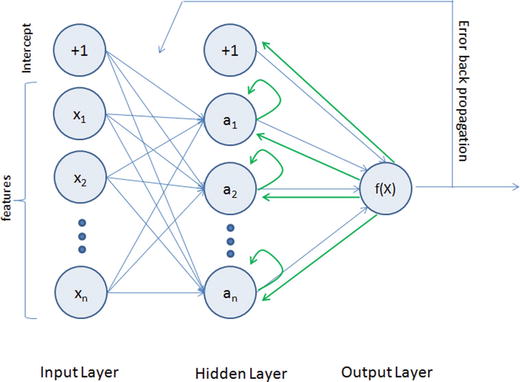
Figure 6-7. Recurrent Neural Network

The previous step’s hidden layer and final outputs are fed back into the network and will be used as input to the next steps’ hidden layer, which means the network will remember the past and it will repeatedly predict what will happen next. The drawback in the general RNN architecture is that it can be memory heavy, and hard to train for long-term temporal dependency (i.e., context of long text should be known at any given stage).

Long Short-Term Memory (LSTM)

LSTM is an implementation of improved RNN architecture to address the issues of general RNN, and it enables long-range dependencies. It is designed to have better memory through linear memory cells surrounded by a set of gate units used to control the flow of information, when information should enter the memory, when to forget, and when to output. It uses no activation function within its recurrent components, thus the gradient term does not vanish with back propagation. Figure 6-8 gives a comparison of simple multilayer perceptron vs. RNN vs. LSTM.

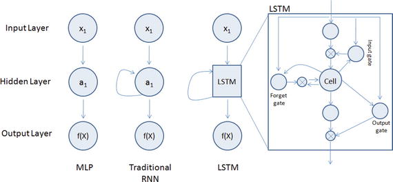
Figure 6-8. Simple MLP vs RNN vs LSTM

Please refer to Table 6-3 below to understand the key LSTM component formulas.

Table 6-3. LSTM Components

LSTM Component	Formula
Input gate layer: This decides which values to store in the cell state.	it = sigmoid(wixt + uiht-1 + bi)
Forget gate layer: As the name suggested this decides what information to throw away from the cell state.	ft = sigmoid(Wfxt + Ufht-1 + bf)
Output gate layer: Create a vector of values that can be added to the cell state.	Ot = sigmoid(Woxt + uiht-1 + bo)
Memory cell state vector.	ct = ft o ct-1+ ito * hyperbolic tangent(Wcxt + ucht-1 + bc)

Let’s look at an example of IMDB dataset that has a labeled sentiment (positive/negative) for movie reviews. The reviews have been preprocessed, and encoded as sequence of word indexes. See Listing 6-14.

Listing 6-14. Example code for Keras LSTM

import numpy as np
np.random.seed(2017)  # for reproducibility

from keras.preprocessing import sequence
from keras.models import Sequential
from keras.layers import Dense, Activation, Embedding
from keras.layers import LSTM
from keras.datasets import imdb

max_features = 20000
maxlen = 80  # cut texts after this number of words (among top max_features most common words)
batch_size = 32

# Load data
(X_train, y_train), (X_test, y_test) = imdb.load_data(nb_words=max_features)
print(len(X_train), 'train sequences')
print(len(X_test), 'test sequences')

print('Pad sequences (samples x time)')
X_train = sequence.pad_sequences(X_train, maxlen=maxlen)
X_test = sequence.pad_sequences(X_test, maxlen=maxlen)
print('X_train shape:', X_train.shape)
print('X_test shape:', X_test.shape)
#----output----
(25000, 'train sequences')
(25000, 'test sequences')
Pad sequences (samples x time)
('X_train shape:', (25000, 80))
('X_test shape:', (25000, 80))

#Model configuration
model = Sequential()
model.add(Embedding(max_features, 128, dropout=0.2))
model.add(LSTM(128, dropout_W=0.2, dropout_U=0.2))  # try using a GRU instead, for fun
model.add(Dense(1))
model.add(Activation('sigmoid'))

# try using different optimizers and different optimizer configs
model.compile(loss='binary_crossentropy', optimizer='adam', metrics=['accuracy'])

#Train
model.fit(X_train, y_train, batch_size=batch_size, nb_epoch=5,
#----output----
validation_data=(X_test, y_test))
Train on 25000 samples, validate on 25000 samples
Epoch 1/5
25000/25000 - 328s - loss: 0.5293 - acc: 0.7332 - val_loss: 0.4101 - val_acc: 0.8206
Epoch 2/5
25000/25000 - 305s - loss: 0.3805 - acc: 0.8354 - val_loss: 0.3814 - val_acc: 0.8297
Epoch 3/5
25000/25000 - 611s - loss: 0.3024 - acc: 0.8746 - val_loss: 0.4037 - val_acc: 0.8343
Epoch 4/5
25000/25000 - 352s - loss: 0.2454 - acc: 0.9016 - val_loss: 0.4397 - val_acc: 0.8304
Epoch 5/5
25000/25000 - 471s - loss: 0.2083 - acc: 0.9164 - val_loss: 0.4175 - val_acc: 0.8342
25000/25000 - 99s
Test score: 0.417513472309
Test accuracy: 0.83424

# Evaluate
train_score, train_acc = model.evaluate(X_train, y_train, batch_size=batch_size)
test_score, test_acc = model.evaluate(X_test, y_test, batch_size=batch_size)

print 'Train score:', train_score
print 'Train accuracy:', train_acc

print 'Test score:', test_score
print 'Test accuracy:', test_acc
#----output----
25000/25000 [==============================] - 83s
25000/25000 [==============================] - 83s
Train score: 0.0930857129323
Train accuracy: 0.97228
Test score: 0.417513472309
Test accuracy: 0.83424

Transfer Learning

Based on our past experience, we humans can learn a new skill easily. We are more efficient in learning, particularly if the task in hand is similar to what we have done in the past, for example, learning a new programming language for a computer professional or driving a new type of vehicle for a seasoned driver is relatively easy based on our past experience.

Transfer learning is an area in machine learning that aims to utilize the knowledge gained while solving one problem to solve a different but related problem. See Figure 6-9.

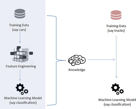
Figure 6-9. Transfer Learning

Nothing better than understanding through example, so let’s train a simple CNN model of two level layers, that is, a feature layer and a classification layer on the first 5 digits (0 to 4) of the MNIST dataset, then apply transfer learning to freeze the features layer and fine-tune dense layers for the classification of digits 5 to 9. See Listing 6-15.

Listing 6-15. Example code for transfer learning

import numpy as np
np.random.seed(2017)  # for reproducibility

from keras.datasets import mnist
from keras.models import Sequential
from keras.layers import Dense, Dropout, Activation, Flatten
from keras.layers import Convolution2D, MaxPooling2D
from keras.utils import np_utils
from keras import backend as K

batch_size = 128
nb_classes = 5
nb_epoch = 5

# input image dimensions
img_rows, img_cols = 28, 28

# number of convolutional filters to use
nb_filters = 32

# size of pooling area for max pooling
pool_size = 2

# convolution kernel size
kernel_size = 3

input_shape = (img_rows, img_cols, 1)
# the data, shuffled and split between train and test sets
(X_train, y_train), (X_test, y_test) = mnist.load_data()

# create two datasets one with digits below 5 and one with 5 and above
X_train_lt5 = X_train[y_train < 5]
y_train_lt5 = y_train[y_train < 5]
X_test_lt5 = X_test[y_test < 5]
y_test_lt5 = y_test[y_test < 5]

X_train_gte5 = X_train[y_train >= 5]
y_train_gte5 = y_train[y_train >= 5] - 5  # make classes start at 0 for
X_test_gte5 = X_test[y_test >= 5]         # np_utils.to_categorical
y_test_gte5 = y_test[y_test >= 5] - 5

# Train model for digits 0 to 4
def train_model(model, train, test, nb_classes):
    X_train = train[0].reshape((train[0].shape[0],) + input_shape)
    X_test = test[0].reshape((test[0].shape[0],) + input_shape)
    X_train = X_train.astype('float32')
    X_test = X_test.astype('float32')
    X_train /= 255
    X_test /= 255
    print('X_train shape:', X_train.shape)
    print(X_train.shape[0], 'train samples')
    print(X_test.shape[0], 'test samples')

    # convert class vectors to binary class matrices
    Y_train = np_utils.to_categorical(train[1], nb_classes)
    Y_test = np_utils.to_categorical(test[1], nb_classes)

    model.compile(loss='categorical_crossentropy',
                  optimizer='adadelta',
                  metrics=['accuracy'])

    model.fit(X_train, Y_train,
              batch_size=batch_size, nb_epoch=nb_epoch,
              verbose=1,
              validation_data=(X_test, Y_test))
    score = model.evaluate(X_test, Y_test, verbose=0)
    print('Test score:', score[0])
    print('Test accuracy:', score[1])

# define two groups of layers: feature (convolutions) and classification (dense)
feature_layers = [
    Convolution2D(nb_filters, kernel_size, kernel_size,
                  border_mode='valid',
                  input_shape=input_shape),
    Activation('relu'),
    Convolution2D(nb_filters, kernel_size, kernel_size),
    Activation('relu'),
    MaxPooling2D(pool_size=(pool_size, pool_size)),
    Dropout(0.25),
    Flatten(),
]
classification_layers = [
    Dense(128),
    Activation('relu'),
    Dropout(0.5),
    Dense(nb_classes),
    Activation('softmax')
]

# create complete model
model = Sequential(feature_layers + classification_layers)

# train model for 5-digit classification [0..4]
train_model(model, (X_train_lt5, y_train_lt5), (X_test_lt5, y_test_lt5), nb_classes)
#----output----
('X_train shape:', (30596, 28, 28, 1))
(30596, 'train samples')
(5139, 'test samples')
Train on 30596 samples, validate on 5139 samples
Epoch 1/5
30596/30596 [==============================] - 57s - loss: 0.2125 - acc: 0.9332 - val_loss: 0.0504 - val_acc: 0.9837
Epoch 2/5
30596/30596 [==============================] - 59s - loss: 0.0734 - acc: 0.9787 - val_loss: 0.0266 - val_acc: 0.9914
Epoch 3/5
30596/30596 [==============================] - 63s - loss: 0.0510 - acc: 0.9854 - val_loss: 0.0189 - val_acc: 0.9940
Epoch 4/5
30596/30596 [==============================] - 64s - loss: 0.0404 - acc: 0.9883 - val_loss: 0.0178 - val_acc: 0.9942
Epoch 5/5
30596/30596 [==============================] - 67s - loss: 0.0340 - acc: 0.9901 - val_loss: 0.0226 - val_acc: 0.9928
('Test score:', 0.022608739081115953)
('Test accuracy:', 0.99280015567230984)

Transfer existing trained model on 0 to 4 to build model for digits 5 to 9

# freeze feature layers and rebuild model
for layer in feature_layers:
    layer.trainable = False

# transfer: train dense layers for new classification task [5..9]
train_model(model, (X_train_gte5, y_train_gte5), (X_test_gte5, y_test_gte5), nb_classes)
#----output----
('X_train shape:', (29404, 28, 28, 1))
(29404, 'train samples')
(4861, 'test samples')
Train on 29404 samples, validate on 4861 samples
Epoch 1/5
29404/29404 [==============================] - 26s - loss: 0.4097 - acc: 0.8762 - val_loss: 0.1096 - val_acc: 0.9677
Epoch 2/5
29404/29404 [==============================] - 26s - loss: 0.1314 - acc: 0.9587 - val_loss: 0.0664 - val_acc: 0.9790
Epoch 3/5
29404/29404 [==============================] - 26s - loss: 0.0975 - acc: 0.9694 - val_loss: 0.0499 - val_acc: 0.9856
Epoch 4/5
29404/29404 [==============================] - 26s - loss: 0.0786 - acc: 0.9760 - val_loss: 0.0424 - val_acc: 0.9866
Epoch 5/5
29404/29404 [==============================] - 26s - loss: 0.0690 - acc: 0.9794 - val_loss: 0.0386 - val_acc: 0.9866
('Test score:', 0.038644227712815393)
('Test accuracy:', 0.98662826567857609)

Notice that we got 99.8% test accuracy after five epochs for the first five digits classifier and 99.2% for the last five digits after transfer and fine-tuning.

Reinforcement Learning

Reinforcement learning is a goal-oriented learning method based on interaction with its environment. The objective is getting an agent to act in an environment in order to maximize its rewards. Here the agent is an intelligent program, and environment is the external condition. See Figure 6-10.

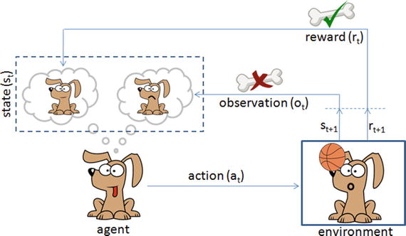
Figure 6-10. Reinforcement learning is like teaching your dog a trick

Let’s consider an example of a predefined system for teaching a new trick to a dog, where you do not have to tell the dog what to do. However, you can reward the dog, if it does it right or punish if it does wrong. With every step, it has to remember what made it get the reward or punishment; this is commonly known as a credit assignment problem. Similarly, we can train a computer agent such that its objective is to take action to move from state st to state st+1 and find behavior function to maximize the expected sum of discounted rewards and map the states to actions. According to the paper published by Deepmind Technologies in 2013, the Q-learning rule for updating status is given by: Q[s,a]_new = Q[s,a]_prev + α * (r + ƴ*max(s,a) – Q[s,a]_prev), where

α is the learning rate,

r is reward for latest action,

ƴ is the discounted factor, and

max(s,a) is the estimate of new value from best action.

If the optimal value Q[s,a] of the sequence s’ at the next time step was known for all possible actions a’, then the optimal strategy is to select the action a’ maximizing the expected value of r + ƴ*max(s,a) – Q[s,a]_prev.

Let’s consider an example where an agent is trying to come out of a maze. It can move one random square or area in any direction, and get a reward if exits. The most common way to formalize a reinforcement problem is to represent it as a Markov decision process. Assume the agent is in state b (maze area) and the target is to reach state f. So within one step agent can reach from b to f, let’s put a reward of 100 (otherwise 0) for links between nodes that allows agents to reach target state. See Figure 6-11 and Listing 6-16.

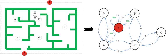
Figure 6-11. Left: Maze with 5 states, Right: Markov Decision process

Listing 6-16. Example code for q-learning

import numpy as np
import matplotlib.pyplot as plt
from matplotlib.collections import LineCollection

# defines the reward/link connection graph
R = np.array([[-1, -1, -1, -1,  0,  -1],
              [-1, -1, -1,  0, -1, 100],
              [-1, -1, -1,  0, -1,  -1],
              [-1,0,  0, -1,  0,  -1],
              [ 0, -1, -1,  0, -1, 100],
              [-1,  0, -1, -1,  0, 100]]).astype("float32")
Q = np.zeros_like(R)

The -1’s in the table means there isn’t a link between nodes. For example, State ‘a’ cannot go to State ‘b’.

# learning parameter
gamma = 0.8

# Initialize random_state
initial_state = randint(0,4)

# This function returns all available actions in the state given as an argument
def available_actions(state):
    current_state_row = R[state,]
    av_act = np.where(current_state_row >= 0)[1]
    return av_act

# This function chooses at random which action to be performed within the range
# of all the available actions.
def sample_next_action(available_actions_range):
    next_action = int(np.random.choice(available_act,1))
    return next_action

# This function updates the Q matrix according to the path selected and the Q
# learning algorithm
def update(current_state, action, gamma):

    max_index = np.where(Q[action,] == np.max(Q[action,]))[1]

    if max_index.shape[0] > 1:
        max_index = int(np.random.choice(max_index, size = 1))
    else:
        max_index = int(max_index)
    max_value = Q[action, max_index]

    # Q learning formula
    Q[current_state, action] = R[current_state, action] + gamma * max_value

# Get available actions in the current state
available_act = available_actions(initial_state)

# Sample next action to be performed
action = sample_next_action(available_act)

# Train over 100 iterations, re-iterate the process above).
for i in range(100):
    current_state = np.random.randint(0, int(Q.shape[0]))
    available_act = available_actions(current_state)
    action = sample_next_action(available_act)
    update(current_state,action,gamma)

# Normalize the "trained" Q matrix
print "Trained Q matrix: \n", Q/np.max(Q)*100

# Testing
current_state = 2
steps = [current_state]

while current_state != 5:
    next_step_index = np.where(Q[current_state,] == np.max(Q[current_state,]))[1]
    if next_step_index.shape[0] > 1:
        next_step_index = int(np.random.choice(next_step_index, size = 1))
    else:
        next_step_index = int(next_step_index)
    steps.append(next_step_index)
    current_state = next_step_index

# Print selected sequence of steps
print "Best sequence path: ", steps
#----output----
Best sequence path:  [2, 3, 1, 5]

Endnotes

In this chapter you have learned briefly about various topics of deep learning techniques using artificial neural networks, starting from single perceptron, multilayer perceptron, to more complex forms of deep neural networks such as CNN / RNN. You have learned about the various issues associated with image data and how researchers have tried to mimic the human brain for building models that can solve complex problems related to computer vision and text mining using the convolution neural network and recurrent neural network respectively. You also learned how autoencoders can be used to compress / de-compress data or remove noise from image data. You learned about the widely popular RBN, which can learn the probabilistic distribution in the input data enabling us to build better models. You learned about the transfer learn that helps us to use the knowledge from one model to another model of a similar nature. Finally, we briefly looked at a simple example of reinforcement learning using q-learning. Congratulations! With this you have reached the end of your six-step expedition of mastering machine learning.