
One of the key areas of artificial intelligence is Natural Language Processing (NLP) or text mining as it is generally known that deals with teaching computers how to extract meaning from text. Over the last two decades, with the explosion of the Internet world and rise of social media, there is plenty of valuable data being generated in the form of text. The process of unearthing meaningful patterns from text data is called Text Mining. In this chapter you’ll learn the high-level text mining process overview, key concepts, and common techniques involved.
Apart from scikit-learn, there is a number of established NLP-focused libraries available for Python, and the number has been growing over time. Refer to Table 5-1 for the most popular libraries based on their number of contributors as of 2016.
Table 5-1. Python popular text mining libraries
Package Name | # of contributors (2016) | License | Description |
|---|---|---|---|
NLTK | 187 | Apache | It’s the most popular and widely used toolkit predominantly built to support research and development of NLP. |
Gensim | 154 | LGPL-2 | Mainly built for large corpus topic modeling, document indexing, and similarity retrieval., |
spaCy | 68 | MIT | Built using Python + Cython for efficient production implementation of NLP concepts. |
Pattern | 20 | BSD-3 | It’s a web mining module for Python with capabilities included for scraping, NLP, machine learning and network analysis/visualization. |
Polyglot | 13 | GPL-3 | This is a multilingual text processing toolkit and supports massive multilingual applications. |
Textblob | 11 | MIT | It’s a wrapper around NLTK and Pattern libraries for easy accessibility of their capabilities. Suitable for fast prototyping. |
Note
Another well-known library is Stanford CoreNLP, a suite of the Java-based toolkit. There are number of Python wrappers available for the same; however, the number of contributors for these wrappers is on the lower side as of now .
Text Mining Process Overview
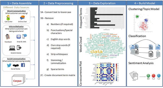
Figure 5-1. Text Mining Process Overview
The overall text mining process can be broadly categorized into four phases .
Text Data Assemble
Text Data Preprocessing
Data Exploration or Visualization
Model Building
Data Assemble (Text)
It is observed that 70% of data available to any business is unstructured. The first step is collating unstructured data from different sources such as open-ended feedback, phone calls, email support, online chat and social media networks like Twitter, LinkedIn, and Facebook. Assembling these data and applying mining/machine learning techniques to analyze them provides valuable opportunities for organizations to build more power into customer experience.
There are several libraries available for extracting text content from different formats discussed above. By far the best library that provides a simple and single interface for multiple formats is ‘textract’ (open source MIT license). Note that as of now this library/package is available for Linux, Mac OS but not Windows. Table 5-2 shows a list of supported formats .
Table 5-2. textract supported formats
Format | Supported Via | Additional Info |
|---|---|---|
.csv / .eml / .json / .odt / .txt / | Python built-ins | |
.doc | Antiword | |
.docx | Python-docx | |
.epub | Ebooklib | |
.gif / .jpg / .jpeg / .png / .tiff / .tif | tesseract-ocr | |
.html / .htm | Beautifulsoup4 | |
.mp3 / .ogg / .wav | SpeechRecongnition and sox | URL 1: https://pypi.python.org/pypi/SpeechRecognition/ URL 2: http://sox.sourceforge.net/ |
.msg | msg-extractor | |
pdftotext and pdfminer.six | ||
.pptx | Python-pptx | |
.ps | ps2text | |
.rtf | Unrtf | |
.xlsx / .xls | Xlrd |
Let’s look at the code for the most widespread formats in the business world: pdf, jpg, and audio file . Note that extracting text from other formats is also relatively simple. See Listing 5-1.
Listing 5-1. Example code for extracting data from pdf, jpg, audio
# You can read/learn more about latest updates about textract on their official documents site at http://textract.readthedocs.io/en/latest/import textract# Extracting text from normal pdftext = textract.process('Data/PDF/raw_text.pdf', language='eng')# Extracting text from two columned pdftext = textract.process('Data/PDF/two_column.pdf', language='eng')# Extracting text from scanned text pdftext = textract.process('Data/PDF/ocr_text.pdf', method='tesseract', language='eng')# Extracting text from jpgtext = textract.process('Data/jpg/raw_text.jpg', method='tesseract', language='eng')# Extracting text from audio filetext = textract.process('Data/wav/raw_text.wav', language='eng')
Social Media
Did you know that Twitter, the online news and social networking service provider, has 320 million users, with an average of 42 million active tweets every day! (Source: Global social media research summary 2016 by smartinsights).
Let’s understand how to explore the rich information of social media (I’ll consider Twitter as an example) to explore what is being spoken about a chosen topic. Most of these forums provide API for developers to access the posts. See Figure 5-2.
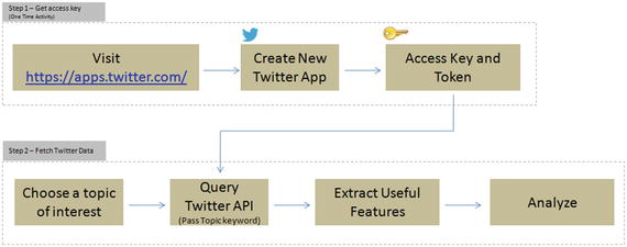
Figure 5-2. Pulling Twitter posts for analysis
Step 1 – Get Access Key (One-Time Activity)
Follow the below steps to set up a new Twitter app to get consumer/access key, secret, and token (do not share the key token with unauthorized persons).
Click on ‘Create New App’
Fill the required information and click on ‘Create your Twitter Application’
You’ll get the access details under ‘Keys and Access Tokens’ tab
Step 2 – Fetching Tweets
Once you have the authorization secret and access tokens, you can use the below code in Listing 5-2 to establish the connection.
Listing 5-2. Twitter authentication
#Import the necessary methods from tweepy libraryimport tweepyfrom tweepy.streaming import StreamListenerfrom tweepy import OAuthHandlerfrom tweepy import Stream#provide your access details belowaccess_token = "Your token goes here"access_token_secret = "Your token secret goes here"consumer_key = "Your consumer key goes here"consumer_secret = "Your consumer secret goes here"# establish a connectionauth = tweepy.auth.OAuthHandler(consumer_key, consumer_secret)auth.set_access_token(access_token, access_token_secret)api = tweepy.API(auth)
Let’s assume that you would like to understand what is being said about the iPhone 7 and its camera feature. So let’s pull the most recent 10 posts.
Note
You can pull historic user posts about a topic for a max of 10 to 15 days only, depending on the volume of the posts.
#fetch recent 10 tweets containing words iphone7, camerafetched_tweets = api.search(q=['iPhone 7','iPhone7','camera'], result_type='recent', lang='en', count=10)print “Number of tweets: ”,len(fetched_tweets)#----output----Number of tweets: 10# Print the tweet textfor tweet in fetched_tweets:print 'Tweet ID: ', tweet.idprint 'Tweet Text: ', tweet.text, '\n'#----output----Tweet ID: 825155021390049281Tweet Text: RT @volcanojulie: A Tau Emerald dragonfly. The iPhone 7 camera is exceptional!#nature #insect #dragonfly #melbourne #australia #iphone7 #...Tweet ID: 825086303318507520Tweet Text: Fuzzy photos? Protect your camera lens instantly with #iPhone7 Full Metallic Case. Buy now! https://t.co/d0dX40BHL6 https://t.co/AInlBoreht
You can capture useful features onto a dataframe for further analysis. See Listing 5-3.
Listing 5-3. Save features to dataframe
# function to save required basic tweets info to a dataframedef populate_tweet_df(tweets):#Create an empty dataframedf = pd.DataFrame()df['id'] = list(map(lambda tweet: tweet.id, tweets))df['text'] = list(map(lambda tweet: tweet.text, tweets))df['retweeted'] = list(map(lambda tweet: tweet.retweeted, tweets))df['place'] = list(map(lambda tweet: tweet.user.location, tweets))df['screen_name'] = list(map(lambda tweet: tweet.user.screen_name, tweets))df['verified_user'] = list(map(lambda tweet: tweet.user.verified, tweets))df['followers_count'] = list(map(lambda tweet: tweet.user.followers_count, tweets))df['friends_count'] = list(map(lambda tweet: tweet.user.friends_count, tweets))# Highly popular user's tweet could possibly seen by large audience, so lets check the popularity of userdf['friendship_coeff'] = list(map(lambda tweet: float(tweet.user.followers_count)/float(tweet.user.friends_count), tweets))return dfdf = populate_tweet_df(fetched_tweets)print df.head(10)#---output----id text0 825155021390049281 RT @volcanojulie: A Tau Emerald dragonfly. The...1 825086303318507520 Fuzzy photos? Protect your camera lens instant...2 825064476714098690 RT @volcanojulie: A Tau Emerald dragonfly. The...3 825062644986023936 RT @volcanojulie: A Tau Emerald dragonfly. The...4 824935025217040385 RT @volcanojulie: A Tau Emerald dragonfly. The...5 824933631365779458 A Tau Emerald dragonfly. The iPhone 7 camera i...6 824836880491483136 The camera on the IPhone 7 plus is fucking awe...7 823805101999390720 'Romeo and Juliet' Ad Showcases Apple's iPhone...8 823804251117850624 iPhone 7 Images Show Bigger Camera Lens - I ha...9 823689306376196096 RT @computerworks5: Premium HD Selfie Stick &a...retweeted place screen_name verified_user0 False Melbourne, Victoria MonashEAE False1 False California, USA ShopNCURV False2 False West Islip, Long Island, NY FusionWestIslip False3 False 6676 Fresh Pond Rd Queens, NY FusionRidgewood False4 False Iphone7review False5 False Melbourne; Monash University volcanojulie False6 False Hollywood, FL Hbk_Mannyp False7 False Toronto.NYC.the Universe AaronRFernandes False8 False Lagos, Nigeria moyinoluwa_mm False9 False Iphone7review Falsefollowers_count friends_count friendship_coeff0 322 388 0.8298971 279 318 0.8773582 13 193 0.0673583 45 218 0.2064224 199 1787 0.1113605 398 551 0.7223236 57 64 0.8906257 18291 7 2613.0000008 780 302 2.5827819 199 1787 0.111360
Instead of a topic you can also choose a screen_name focused on a topic; let’s look at the posts by the screen name Iphone7review. See Listing 5-4.
Listing 5-4. Example code for extracting tweets based on screen name
# For help about api look here http://tweepy.readthedocs.org/en/v2.3.0/api.htmlfetched_tweets = api.user_timeline(id='Iphone7review', count=5)# Print the tweet textfor tweet in fetched_tweets:print 'Tweet ID: ', tweet.idprint 'Tweet Text: ', tweet.text, '\n'#----output----Tweet ID: 825169063676608512Tweet Text: RT @alicesttu: iPhone 7S to get Samsung OLED display next year #iPhone https://t.co/BylKbvXgAG #iphoneTweet ID: 825169047138533376Tweet Text: Nothing beats the Iphone7! Who agrees? #Iphone7 https://t.co/e03tXeLOao
Glancing through the posts quickly can generally help you conclude that there are positive comments about the camera feature of iPhone 7.
Data Preprocessing (Text)
This step deals with cleansing the consolidated text to remove noise to ensure efficient syntactic, semantic text analysis for deriving meaningful insights from text. Some common cleaning steps are briefed below.
Convert to Lower Case and Tokenize
Here, all the data is converted into lowercase. This is carried out to prevent words like “LIKE” or “Like” being interpreted as different words. Python provides a function lower() to convert text to lowercase.
Tokenizing is the process of breaking a large set of texts into smaller meaningful chunks such as sentences, words, and phrases.
Sentence Tokenizing
The NLTK library provides a sent_tokenize for sentence-level tokenizing, which uses a pre-trained model PunktSentenceTokenize, to determine punctuation and characters marking the end of sentence for European languages. See Listing 5-5.
Listing 5-5. Example code for sentence tokenization
import nltkfrom nltk.tokenize import sent_tokenizetext='Statistics skills, and programming skills are equally important for analytics. Statistics skills, and domain knowledge are important for analytics. I like reading books and travelling.'sent_tokenize_list = sent_tokenize(text)print(sent_tokenize_list)#----output----['Statistics skills, and programming skills are equally important for analytics.', 'Statistics skills, and domain knowledge are important for analytics.', 'I like reading books and travelling.']
There are a total of 17 European languages that NLTK supports for sentence tokenization. You can load the tokenized model for specific language saved as a pickle file as part of nltk.data. see Listing 5-6.
Listing 5-6. Sentence tokenization for European languages
import nltk.dataspanish_tokenizer = nltk.data.load('tokenizers/punkt/spanish.pickle')spanish_tokenizer.tokenize('Hola. Esta es una frase espanola.')#----output----['Hola.', 'Esta es una frase espanola.']
Word Tokenizing
The word_tokenize function of NLTK is a wrapper function that calls tokenize by the TreebankWordTokenizer. See Listing 5-7.
Listing 5-7. Example code for word tokenizing
from nltk.tokenize import word_tokenizeprint word_tokenize(text)# Another equivalent call method using TreebankWordTokenizerfrom nltk.tokenize import TreebankWordTokenizertokenizer = TreebankWordTokenizer()print tokenizer.tokenize(text)#----output----
[‘Statistics’, ‘skills’, ‘ , ’, ‘and’, ‘programming’, ‘skills’, ‘are’, ‘equally’, ‘important’, ‘for’, ‘analytics’, ‘ . ’, ‘Statistics’, ‘skills’, ‘ , ’, ‘and’, ‘domain’, ‘knowledge’, ‘are’, ‘important’, ‘for’, ‘analytics’, ‘ . ‘, ‘I’, ‘like’, ‘reading’, ‘books’, ‘and’, ‘travelling’, ‘ . ’]
Removing Noise
You should remove all information that is not comparative or relevant to text analytics. These can be seen as noise to the text analytics. Most common noises are numbers, punctuations, stop words, white space, etc
Numbers: Numbers are removed as they may not be relevant and not hold valuable information. See Listing 5-8.
Listing 5-8. Example code for removing noise from text
def remove_numbers(text):return re.sub(r'\d+', '', text)text = 'This is a sample English sentence, \n with whitespace and numbers 1234!'print 'Removed numbers: ', remove_numbers(text)#----output----Removed numbers: This is a sample English sentence,with whitespace and numbers !
Punctuation: It is to be removed for better identifying each word and remove punctuation characters from the dataset. For example “like” and “like” or “coca-cola” and “cocacola” would be interpreted as different words if the punctuation was not removed. See Listing 5-9.
Listing 5-9. Example code for removing punctuation from text
import string# Function to remove punctuationsdef remove_punctuations(text):words = nltk.word_tokenize(text)punt_removed = [w for w in words if w.lower() not in string.punctuation]return " ".join(punt_removed)print remove_punctuations('This is a sample English sentence, with punctuations!')#----output----This is a sample English sentence with punctuations
Stop words: Words like “the,” “and,” “or” are uninformative and add unneeded noise to the analysis. For this reason they are removed. See Listing 5-10.
Listing 5-10. Example code for removing stop words from text
from nltk.corpus import stopwords# Function to remove stop wordsdef remove_stopwords(text, lang='english'):words = nltk.word_tokenize(text)lang_stopwords = stopwords.words(lang)stopwords_removed = [w for w in words if w.lower() not in lang_stopwords]return " ".join(stopwords_removed)print remove_stopwords('This is a sample English sentence')#----output----sample English sentence
Note
Remove own stop words (if required) – Certain words could be very commonly used in a particular domain. Along with English stop words, we could instead, or in addition, remove our own stop words. The choice of our own stop word might depend on the domain of discourse and might not become apparent until we’ve done some analysis.
Whitespace: Often in text analytics, an extra whitespace (space, tab, Carriage Return, Line Feed) becomes identified as a word. This anomaly is avoided through a basic programming procedure in this step. See Listing 5-11.
Listing 5-11. Example code for removing whitespace from text
# Function to remove whitespacedef remove_whitespace(text):return " ".join(text.split())text = 'This is a sample English sentence, \n with whitespace and numbers 1234!'print 'Removed whitespace: ', remove_whitespace(text)#----output----Removed whitespace: This is a sample English sentence, with whitespace and numbers 1234!
Part of Speech (PoS) Tagging
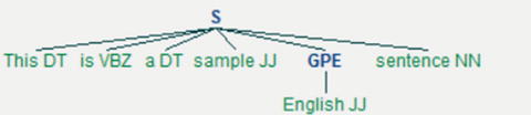
PoS tagging is the process of assigning language-specific parts of speech such as nouns, verbs, adjectives, and adverbs, etc., for each word in the given text.
NLTK supports multiple PoS tagging models, and the default tagger is maxent_treebank_pos_tagger, which uses Penn (Pennsylvania University) Tree bank corpus. The same has 36 possible parts of speech tags, a sentence (S) is represented by the parser as a tree having three children: a noun phrase (NP), a verbal phrase (VP), and the full stop (.). The root of the tree will be S. See Table 5-3 and Listings 5-12 and 5-13.
Table 5-3. NLTK PoS taggers
PoS Tagger | Short Description |
|---|---|
maxent_treebank_pos_tagger | It’s based on Maximum Entropy (ME) classification principles trained on Wall Street Journal subset of the Penn Tree bank corpus. |
BrillTagger | Brill’s transformational rule-based tagger. |
CRFTagger | Conditional Random Fields. |
HiddenMarkovModelTagger | Hidden Markov Models (HMMs) largely used to assign the correct label sequence to sequential data or assess the probability of a given label and data sequence. |
HunposTagge | A module for interfacing with the HunPos open source POS-tagger. |
PerceptronTagger | Based on averaged perceptron technique proposed by Matthew Honnibal. |
SennaTagger | Semantic/syntactic Extraction using a Neural Network Architecture. |
SequentialBackoffTagger | Classes for tagging sentences sequentially, left to right. |
StanfordPOSTagger | Researched and developed at Stanford University. |
TnT | Implementation of ‘TnT - A Statistical Part of Speech Tagger’ by Thorsten Brants. |
Listing 5-12. Example code for PoS, the sentence, and visualize sentence tree
from nltk import chunktagged_sent = nltk.pos_tag(nltk.word_tokenize('This is a sample English sentence'))print tagged_senttree = chunk.ne_chunk(tagged_sent)tree.draw() # this will draw the sentence tree#----output----[('This', 'DT'), ('is', 'VBZ'), ('a', 'DT'), ('sample', 'JJ'), ('English', 'JJ'), ('sentence', 'NN')]
Listing 5-13. Example code for using perceptron tagger and getting help on tags
# To use PerceptronTaggerfrom nltk.tag.perceptron import PerceptronTaggerPT = PerceptronTagger()print PT.tag('This is a sample English sentence'.split())#----output----[('This', 'DT'), ('is', 'VBZ'), ('a', 'DT'), ('sample', 'JJ'), ('English', 'JJ'), ('sentence', 'NN')]# To get help about tagsnltk.help.upenn_tagset('NNP')#----output----NNP: noun, proper, singular
Stemming
It is the process of transforming to the root word, that is, it uses an algorithm that removes common word endings from English words, such as “ly,” “es,” “ed,” and “s.” For example, assuming for an analysis you may want to consider “carefully,” “cared,” “cares,” “caringly” as “care” instead of separate words. There are three widely used stemming algorithms as listed in Figure 5-3. See Listing 5-14.
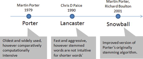
Figure 5-3. Most popular NLTK stemmers
Listing 5-14. Example code for stemming
from nltk import PorterStemmer, LancasterStemmer, SnowballStemmer# Function to apply stemming to a list of wordsdef words_stemmer(words, type="PorterStemmer", lang="english", encoding="utf8"):supported_stemmers = ["PorterStemmer","LancasterStemmer","SnowballStemmer"]if type is False or type not in supported_stemmers:return wordselse:stem_words = []if type == "PorterStemmer":stemmer = PorterStemmer()for word in words:stem_words.append(stemmer.stem(word).encode(encoding))if type == "LancasterStemmer":stemmer = LancasterStemmer()for word in words:stem_words.append(stemmer.stem(word).encode(encoding))if type == "SnowballStemmer":stemmer = SnowballStemmer(lang)for word in words:stem_words.append(stemmer.stem(word).encode(encoding))return " ".join(stem_words)words = 'caring cares cared caringly carefully'print "Original: ", wordsprint "Porter: ", words_stemmer(nltk.word_tokenize(words), "PorterStemmer")print "Lancaster: ", words_stemmer(nltk.word_tokenize(words), "LancasterStemmer")print "Snowball: ", words_stemmer(nltk.word_tokenize(words), "SnowballStemmer")#----output----Original: caring cares cared caringly carefullyPorter: care care care caringli careLancaster: car car car car carSnowball: care care care care care
Lemmatization
It is the process of transforming to the dictionary base form. For this you can use WordNet, which is a large lexical database for English words that are linked together by their semantic relationships. It works as a thesaurus, that is, it groups words together based on their meanings. See Listing 5-15.
Listing 5-15. Example code for lemmatization
from nltk.stem import WordNetLemmatizerwordnet_lemmatizer = WordNetLemmatizer()# Function to apply lemmatization to a list of wordsdef words_lemmatizer(text, encoding="utf8"):words = nltk.word_tokenize(text)lemma_words = []wl = WordNetLemmatizer()for word in words:pos = find_pos(word)lemma_words.append(wl.lemmatize(word, pos).encode(encoding))return " ".join(lemma_words)# Function to find part of speech tag for a worddef find_pos(word):# Part of Speech constants# ADJ, ADJ_SAT, ADV, NOUN, VERB = 'a', 's', 'r', 'n', 'v'# You can learn more about these at http://wordnet.princeton.edu/wordnet/man/wndb.5WN.html#sect3# You can learn more about all the penn tree tags at https://www.ling.upenn.edu/courses/Fall_2003/ling001/penn_treebank_pos.htmlpos = nltk.pos_tag(nltk.word_tokenize(word))[0][1]# Adjective tags - 'JJ', 'JJR', 'JJS'if pos.lower()[0] == 'j':return 'a'# Adverb tags - 'RB', 'RBR', 'RBS'elif pos.lower()[0] == 'r':return 'r'# Verb tags - 'VB', 'VBD', 'VBG', 'VBN', 'VBP', 'VBZ'elif pos.lower()[0] == 'v':return 'v'# Noun tags - 'NN', 'NNS', 'NNP', 'NNPS'else:return 'n'print "Lemmatized: ", words_lemmatizer(words)#----output----Lemmatized: care care care caringly carefullyIn the above case,‘caringly’/’carefully’ are inflected form of care and they are an entry word listed in WordNet Dictoinary so they are retained in their actual form itself.
NLTK English WordNet includes approximately 155,287 words and 117000 synonym sets. For a given word, WordNet includes/provides definition, example, synonyms (group of nouns, adjectives, verbs that are similar), atonyms (opposite in meaning to another), etc. See Listing 5-16.
Listing 5-16. Example code for wordnet
from nltk.corpus import wordnetsyns = wordnet.synsets("good")print "Definition: ", syns[0].definition()print "Example: ", syns[0].examples()synonyms = []antonyms = []# Print synonums and antonyms (having opposite meaning words)for syn in wordnet.synsets("good"):for l in syn.lemmas():synonyms.append(l.name())if l.antonyms():antonyms.append(l.antonyms()[0].name())print "synonyms: \n", set(synonyms)print "antonyms: \n", set(antonyms)#----output----Definition: benefitExample: [u'for your own good', u"what's the good of worrying?"]synonyms:set([u'beneficial', u'right', u'secure', u'just', u'unspoilt', u'respectable', u'good', u'goodness', u'dear', u'salutary', u'ripe', u'expert', u'skillful', u'in_force', u'proficient', u'unspoiled', u'dependable', u'soundly', u'honorable', u'full', u'undecomposed', u'safe', u'adept', u'upright', u'trade_good', u'sound', u'in_effect', u'practiced', u'effective', u'commodity', u'estimable', u'well', u'honest', u'near', u'skilful', u'thoroughly', u'serious'])antonyms:set([u'bad', u'badness', u'ill', u'evil', u'evilness'])
N-grams
One of the important concepts in text mining is n-grams, which are fundamentally a set of co-occurring or continuous sequence of n items from a given sequence of large text. The item here could be words, letters, and syllables. Let’s consider a sample sentence and try to extract n-grams for different values of n. See Listing 5-17.
Listing 5-17. Example code for extracting n-grams from sentence
from nltk.util import ngramsfrom collections import Counter# Function to extract n-grams from textdef get_ngrams(text, n):n_grams = ngrams(nltk.word_tokenize(text), n)return [ ' '.join(grams) for grams in n_grams]text = 'This is a sample English sentence'print "1-gram: ", get_ngrams(text, 1)print "2-gram: ", get_ngrams(text, 2)print "3-gram: ", get_ngrams(text, 3)print "4-gram: ", get_ngrams(text, 4)#----output----1-gram:['This', 'is', 'a', 'sample', 'English', 'sentence']2-gram:['This is', 'is a', 'a sample', 'sample English', 'English sentence']3-gram:['This is a', 'is a sample', 'a sample English', 'sample English sentence']4-gram: ['This is a sample', 'is a sample English', 'a sample English sentence']
Note
1-gram is also called as unigram, 2-gram, and 3-gram as bigram and trigram, respectively.
The N-gram technique is relatively simple and simply increasing the value of n will give us more contexts. It is widely used in the probabilistic language model of predicting the next item in a sequence: for example, search engines use this technique to predict/recommend the possibility of next character/words in the sequence to users as they type. See Listing 5-18.
Listing 5-18. Example code for extracting 2-grams from sentence and store it in a dataframe
text = 'Statistics skills, and programming skills are equally important for analytics. Statistics skills, and domain knowledge are important for analytics'# remove punctuationstext = remove_punctuations(text)# Extracting bigramsresult = get_ngrams(text,2)# Counting bigramsresult_count = Counter(result)# Converting to the result to a data frameimport pandas as pddf = pd.DataFrame.from_dict(result_count, orient='index')df = df.rename(columns={'index':'words', 0:'frequency'}) # Renaming index and column nameprint df#----output----frequencyare equally 1domain knowledge 1skills are 1knowledge are 1programming skills 1are important 1skills and 2for analytics 2and domain 1important for 2and programming 1Statistics skills 2equally important 1analytics Statistics 1
Bag of Words (BoW)
The texts have to be represented as numbers to be able to apply any algorithms. Bag of words is the method where you count the occurrence of words in a document without giving importance to the grammar and the order of words. This can be achieved by creating Term Document Matrix (TDM) . It is simply a matrix with terms as the rows and document names as the columns and a count of the frequency of words as the cells of the matrix. Let’s learn about creating DTM through an example; consider three text documents with some text in it. Sklearn provides good functions under feature_extraction.text to convert a collection of text documents to a matrix of word counts. See Listing 5-19 and Figure 5-4.
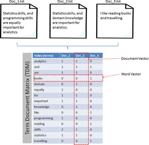
Figure 5-4. Document Term Matrix
Listing 5-19. Creating document term matrix from corpus of sample documents
import osimport pandas as pdfrom sklearn.feature_extraction.text import CountVectorizer# Function to create a dictionary with key as file names and values as text for all files in a given folderdef CorpusFromDir(dir_path):result = dict(docs = [open(os.path.join(dir_path,f)).read() for f in os.listdir(dir_path)],ColNames = map(lambda x: x, os.listdir(dir_path)))return resultdocs = CorpusFromDir('Data/')# Initializevectorizer = CountVectorizer()doc_vec = vectorizer.fit_transform(docs.get('docs'))#create dataFramedf = pd.DataFrame(doc_vec.toarray().transpose(), index = vectorizer.get_feature_names())# Change column headers to be file namesdf.columns = docs.get('ColNames')print df#----output----Doc_1.txt Doc_2.txt Doc_3.txtanalytics 1 1 0and 1 1 1are 1 1 0books 0 0 1domain 0 1 0equally 1 0 0for 1 1 0important 1 1 0knowledge 0 1 0like 0 0 1programming 1 0 0reading 0 0 1skills 2 1 0statistics 1 1 0travelling 0 0 1
Note
Document Term Matrix (DTM) is the transpose of Term Document Matrix. In DTM the rows will be the document names and column headers will be the terms. Both are in the matrix format and useful for carrying out analysis; however TDM is commonly used due to the fact that the number of terms tends to be way larger than the document count. In this case having more rows is better than having a large number of columns.
Term Frequency-Inverse Document Frequency (TF-IDF)
In the area of information retrieval, TF-IDF is a good statistical measure to reflect the relevance of the term to the document in a collection of documents or corpus. Let’s break TF_IDF and apply an example to understand it better. See Listing 5-20.
Term frequency will tell you how frequently a given term appears.
For example, consider a document containing 100 words wherein the word ‘ML’ appears 3 times, then TF (ML) = 3 / 100 =0.03
Document frequency will tell you how important a term is?
Assume we have 10 million documents and the word ML appears in one thousand of these, then DF (ML) = 1000/10,000,000 = 0.0001
To normalize let’s take a log (d/D), that is, log (0.0001) = -4
Quite often D > d and log (d/D) will give a negative value as seen in the above example. So to solve this problem let’s invert the ratio inside the log expression, which is known as Inverse document frequency (IDF). Essentially we are compressing the scale of values so that very large or very small quantities are smoothly compared.
Continuing with the above example, IDF(ML) = log(10,000,000 / 1,000) = 4
TF-IDF is the weight product of quantities, that is, for the above example TF-IDF (ML) = 0.03 * 4 = 0.12
sklearn provides provides a function TfidfVectorizer to calculate TF-IDF for text, however by default it normalizes the term vector using L2 normalization and also IDF is smoothed by adding one to the document frequency to prevent zero divisions.Listing 5-20. Create document term matrix with TF-IDF
from sklearn.feature_extraction.text import TfidfVectorizervectorizer = TfidfVectorizer()doc_vec = vectorizer.fit_transform(docs.get('docs'))#create dataFramedf = pd.DataFrame(doc_vec.toarray().transpose(), index = vectorizer.get_feature_names())# Change column headers to be file namesdf.columns = docs.get('ColNames')print df#----output----Doc_1.txt Doc_2.txt Doc_3.txtanalytics 0.276703 0.315269 0.000000and 0.214884 0.244835 0.283217are 0.276703 0.315269 0.000000books 0.000000 0.000000 0.479528domain 0.000000 0.414541 0.000000equally 0.363831 0.000000 0.000000for 0.276703 0.315269 0.000000important 0.276703 0.315269 0.000000knowledge 0.000000 0.414541 0.000000like 0.000000 0.000000 0.479528programming 0.363831 0.000000 0.000000reading 0.000000 0.000000 0.479528skills 0.553405 0.315269 0.000000statistics 0.276703 0.315269 0.000000travelling 0.000000 0.000000 0.479528
Data Exploration (Text)
In this stage the corpus is explored to understand the common key words, content, relationship, and presence of level of noise. This can be achieved by creating basic statistics and embracing visualization techniques such as word frequency count, word co-occurrence, or correlation plot, etc., which will help us to discover hidden patterns if any.
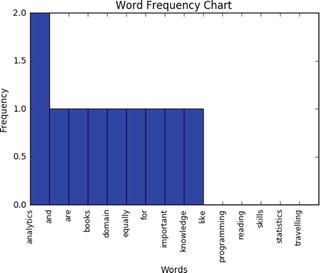
Frequency Chart
This visualization presents a bar chart whose length corresponds to the frequency a particular word occurred. Let’s plot a frequency chart for Doc_1.txt file. See Listing 5-21.
Listing 5-21. Example code for frequency chart
words = df.indexfreq = df.ix[:,0].sort(ascending=False, inplace=False)pos = np.arange(len(words))width=1.0ax=plt.axes(frameon=True)ax.set_xticks(pos)ax.set_xticklabels(words, rotation='vertical', fontsize=9)ax.set_title('Word Frequency Chart')ax.set_xlabel('Words')ax.set_ylabel('Frequency')plt.bar(pos, freq, width, color='b')plt.show()#----output----
Word Cloud
This is a visual representation of text data, which is helpful to get a high-level understanding about the important keywords from data in terms of its occurrence. ‘WordCloud’ package can be used to generate words whose font size relates to its frequency. See Listing 5-22.
Listing 5-22. Example code for wordcloud
from wordcloud import WordCloud# Read the whole text.text = open('Data/Text_Files/Doc_1.txt').read()# Generate a word cloud imagewordcloud = WordCloud().generate(text)# Display the generated image:# the matplotlib way:import matplotlib.pyplot as pltplt.imshow(wordcloud.recolor(random_state=2017))plt.title('Most Frequent Words')plt.axis("off")plt.show()#----output----
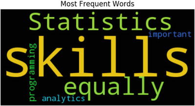
From the above chart we can see that ‘skills’ appear the most number of times comparatively.
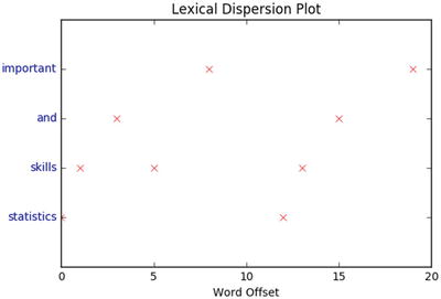
Lexical Dispersion Plot
This plot is helpful to determine the location of a word in a sequence of text sentences. On the x-axis you’ll have word offset numbers and on the y-axis each row is a representation of the entire text and the marker indicates an instance of the word of interest. See Listing 5-23.
Listing 5-23. Example code for lexical dispersion plot
from nltk import word_tokenizedef dispersion_plot(text, words):words_token = word_tokenize(text)points = [(x,y) for x in range(len(words_token)) for y in range(len(words)) if words_token[x] == words[y]]if points:x,y=zip(*points)else:x=y=()plt.plot(x,y,"rx",scalex=.1)plt.yticks(range(len(words)),words,color="b")plt.ylim(-1,len(words))plt.title("Lexical Dispersion Plot")plt.xlabel("Word Offset")plt.show()text = 'statistics skills, and programming skills are equally important for analytics. statistics skills, and domain knowledge are important for analytics'dispersion_plot(text, ['statistics', 'skills', 'and', 'important'])#----output----
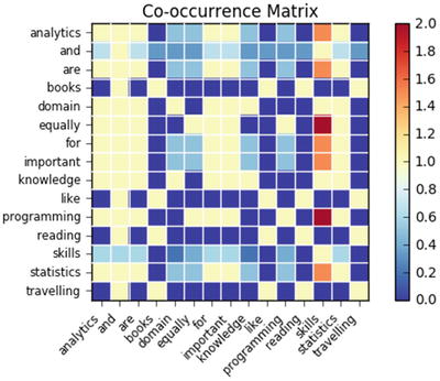
Co-occurrence Matrix
Calculating the co-occurrence between words in a sequence of text will be helpful matrices to explain the relationship between words. A co-occurrence matrix tells us how many times every word has co-occurred with the current word. Further plotting this matrix into a heat map is a powerful visual tool to spot the relationships between words efficiently. See Listing 5-24.
Listing 5-24. Example code for co-occurrence matrix
import statsmodels.api as smimport scipy.sparse as sp# default unigram modelcount_model = CountVectorizer(ngram_range=(1,1))docs_unigram = count_model.fit_transform(docs.get('docs'))# co-occurrence matrix in sparse csr formatdocs_unigram_matrix = (docs_unigram.T * docs_unigram)# fill same word cooccurence to 0docs_unigram_matrix.setdiag(0)# co-occurrence matrix in sparse csr formatdocs_unigram_matrix = (docs_unigram.T * docs_unigram) docs_unigram_matrix_diags = sp.diags(1./docs_unigram_matrix.diagonal())# normalized co-occurence matrixdocs_unigram_matrix_norm = docs_unigram_matrix_diags * docs_unigram_matrix# Convert to a dataframedf = pd.DataFrame(docs_unigram_matrix_norm.todense(), index = count_model.get_feature_names())df.columns = count_model.get_feature_names()# Plotsm.graphics.plot_corr(df, title='Co-occurrence Matrix', xnames=list(df.index))plt.show()#----output----
Model Building
As you might be familiar with by now, model building is the process of understanding and establishing relationships between variables. So far you have learned how to extract text content from various sources, preprocess to remove noise, and perform exploratory analysis to get basic understanding/statistics about the text data in hand. Now you’ll learn to apply machine learning techniques on the processed data to build models.
Text Similarity
A measure that indicates how similar two objects are is described through a distance measure with dimensions represented by features of the objects (here text). A smaller distance indicates a high degree of similarity and vice versa. Note that similarity is highly subjective and dependent on domain or application. For text similarity, it is important to choose the right distance measure to get better results. There are various distance measures available and Euclidian metric is the most common, which is a straight line distance between two points. However a significant amount of research has been carried out in the field of text mining to learn that cosine distance better suits for text similarity.
Let’s look at a simple example to understand similarity better. Consider three documents containing certain simple text keywords and assume that the top two keywords are accident and New York. For the moment ignore other keywords and let’s calculate the similarity of document based on these two keywords frequency. See Table 5-4.
Table 5-4. Sample document term matrix
Document # | Count of ‘Accident’ | Count of ‘New York’ |
|---|---|---|
1 | 2 | 8 |
2 | 3 | 7 |
3 | 7 | 3 |
Plotting the document word vector points on a two-dimensional chart is depicted on Figure 5-5. Notice that the cosine similarity equation is the representation of the angle between the two data points, whereas Euclidian distance is the square root of straight line differences between data points. The cosine similarity equation will result in a value between 0 and 1. The smaller cosine angle results in a bigger cosine value, indicating higher similarity. In this case Euclidean distance will result in a zero. Let’s put the values in the formula to find the similarity between documents 1 and 2.
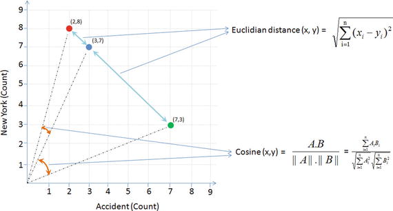
Figure 5-5. Euclidian vs. Cosine
Euclidian distance (doc1, doc2) = 
Cosine (doc1, doc2) =  , where
doc1 = (2,8)
doc2 = (3,7)
doc1 . doc2 = (2*3 + 8*7) = (56 + 6) = 62
||doc1|| = `
||doc2|| = 
Similarly let’s find the similarity between documents 1 and 3. See Figure 5-5.
Euclidian distance (doc1, doc3) =
Cosine (doc1, doc3)= 
According to the cosine equation, documents 1 and 2 are 98% similar; this could mean that these two documents may be talking about ‘New York’. Whereas document 3 can be assumed to be focused more about ‘Accident’, however, there is a mention of ‘New York’ a couple of times resulting in a similarity of 60% between documents 1 and 3.
Let’s apply cosine similarity for the example given in Figure 5-5. See Listing 5-25.
Listing 5-25. Example code for calculating cosine similarity for documents
from sklearn.metrics.pairwise import cosine_similarityprint "Similarity b/w doc 1 & 2: ", cosine_similarity(df['Doc_1.txt'], df['Doc_2.txt'])print "Similarity b/w doc 1 & 3: ", cosine_similarity(df['Doc_1.txt'], df['Doc_3.txt'])print "Similarity b/w doc 2 & 3: ", cosine_similarity(df['Doc_2.txt'], df['Doc_3.txt'])#----output----Similarity b/w doc 1 & 2: [[ 0.76980036]]Similarity b/w doc 1 & 3: [[ 0.12909944]]Similarity b/w doc 2 & 3: [[ 0.1490712]]
Text Clustering
As an example we’ll be using the 20 newsgroups dataset consisting of 18,000+ newsgroup posts on 20 topics. You can learn more about the dataset at http://qwone.com/~jason/20Newsgroups/ . Let’s load the data and check the topic names. See Listing 5-26.
Listing 5-26. Example code for text clustering
from sklearn.datasets import fetch_20newsgroupsfrom sklearn.feature_extraction.text import TfidfVectorizerfrom sklearn.preprocessing import Normalizerfrom sklearn import metricsfrom sklearn.cluster import KMeans, MiniBatchKMeansimport numpy as np# load data and print topic namesnewsgroups_train = fetch_20newsgroups(subset='train')print(list(newsgroups_train.target_names))#----output----['alt.atheism', 'comp.graphics', 'comp.os.ms-windows.misc', 'comp.sys.ibm.pc.hardware', 'comp.sys.mac.hardware', 'comp.windows.x', 'misc.forsale', 'rec.autos', 'rec.motorcycles', 'rec.sport.baseball', 'rec.sport.hockey', 'sci.crypt', 'sci.electronics', 'sci.med', 'sci.space', 'soc.religion.christian', 'talk.politics.guns', 'talk.politics.mideast', 'talk.politics.misc', 'talk.religion.misc']
To keep it simple, let’s filter only three topics. Assume that we do not know the topics, so let’s run a clustering algorithm and examine the keywords of each cluster.
categories = ['alt.atheism', 'comp.graphics', 'rec.motorcycles']dataset = fetch_20newsgroups(subset='all', categories=categories, shuffle=True, random_state=2017)print("%d documents" % len(dataset.data))print("%d categories" % len(dataset.target_names))labels = dataset.targetprint("Extracting features from the dataset using a sparse vectorizer")vectorizer = TfidfVectorizer(stop_words='english')X = vectorizer.fit_transform(dataset.data)print("n_samples: %d, n_features: %d" % X.shape)#----output----2768 documents3 categoriesExtracting features from the dataset using a sparse vectorizern_samples: 2768, n_features: 35311
Latent Semantic Analysis (LSA)
LSA is a mathematical method that tries to bring out latent relationships within a collection of documents. Rather than looking at each document isolated from the others, it looks at all the documents as a whole and the terms within them to identify relationships. Let’s perform LSA by running SVD on the data to reduce the dimensionality.
SVD of matrix A = U * ∑ * VTr = rank of matrix XU = column orthonormal m * r matrix∑ = diagonal r * r matrix with singular value sorted in descending orderV = column orthonormal r * n matrixIn our case we have 3 topics, 2768 documents and 35311 word vocabulary.* Original matrix = 2768*35311 ∼ 108* SVD = 3*2768 + 3 + 3*35311 ∼ 105.3
Resulted SVD is taking approximately 460 times less space than original matrix.
Note
“Latent Semantic Analysis (LSA)” and “Latent Semantic Indexing (LSI)” is the same thing, with the latter name being used sometimes when referring specifically to indexing a collection of documents for search (“Information Retrieval”). See Figure 5-6 and Listing 5-27.
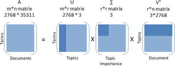
Figure 5-6. Singular Value Decomposition
Listing 5-27. Example code for LSA through SVD
from sklearn.decomposition import TruncatedSVD# Lets reduce the dimensionality to 2000svd = TruncatedSVD(2000)lsa = make_pipeline(svd, Normalizer(copy=False))X = lsa.fit_transform(X)explained_variance = svd.explained_variance_ratio_.sum()print("Explained variance of the SVD step: {}%".format(int(explained_variance * 100)))#----output----Explained variance of the SVD step: 95%
Let’s run k-means clustering on the SVD output as shown in Listing 5-28.
Listing 5-28. k-means clustering on SVD dataset
from __future__ import print_functionkm = KMeans(n_clusters=3, init='k-means++', max_iter=100, n_init=1)# Scikit learn provides MiniBatchKMeans to run k-means in batch mode suitable for a very large corpus# km = MiniBatchKMeans(n_clusters=5, init='k-means++', n_init=1, init_size=1000, batch_size=1000)print("Clustering sparse data with %s" % km)km.fit(X)print("Top terms per cluster:")original_space_centroids = svd.inverse_transform(km.cluster_centers_)order_centroids = original_space_centroids.argsort()[:, ::-1]terms = vectorizer.get_feature_names()for i in range(3):print("Cluster %d:" % i, end='')for ind in order_centroids[i, :10]:print(' %s' % terms[ind], end='')print()#----output----Top terms per cluster:Cluster 0: edu graphics university god subject lines organization com posting ukCluster 1: com bike edu dod ca writes article sun like organizationCluster 2: keith sgi livesey caltech com solntze wpd jon edu sandvik
Topic Modeling
Topic modeling algorithms enable you to discover hidden topical patterns or thematic structure in a large collection of documents. The most popular topic modeling techniques are Latent Dirichlet Allocation (LDA) and Non-negative Matrix Factorization (NMF).
Latent Dirichlet Allocation (LDA)
LDA was presented by David Blei, Andrew Ng, and Michael I.J in 2003 as a graphical model. See Figure 5-7.
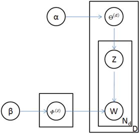
Figure 5-7. LDA graph model
LDA is given by 
Where, F(z) = word distribution for topic,
a = Dirichlet parameter prior the per-document topic distribution,
b = Dirichlet parameter prior the per-document word distribution,
q(d) = topic distribution for a document
LDA’s objective is to maximize separation between means of projected topics and minimize variance within each projected topic. So LDA defines each topic as a bag of words by carrying out three steps described below.
Step 1: Initialize k clusters and assign each word in the document to one of the k topics.
Step 2: Re-assign word to new topic based on a) how is the proportion of words for a document to a topic, and b) how is the proportion of a topic widespread across all documents.
Step 3: Repeat step 2 until coherent topics result. See Figure 5-8 and Listing 5-29.
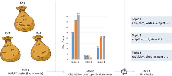
Figure 5-8. Latent Dirichlet Allocation (LDA)
Listing 5-29. Example code for LDA
from sklearn.decomposition import LatentDirichletAllocation# continuing with the 20 newsgroup dataset and 3 topicstotal_topics = 3lda = LatentDirichletAllocation(n_topics=total_topics,max_iter=100,learning_method='online',learning_offset=50.,random_state=2017)lda.fit(X)feature_names = np.array(vectorizer.get_feature_names())for topic_idx, topic in enumerate(lda.components_):print("Topic #%d:" % topic_idx)print(" ".join([feature_names[i] for i in topic.argsort()[:-20 - 1:-1]]))#----output----Topic #0:edu com writes subject lines organization article posting university nntp host don like god uk ca just bike know graphicsTopic #1:anl elliptical maier michael_maier qmgate separations imagesetter 5298 unscene appreshed linotronic l300 iici amnesia glued veiw halftone 708 252 dotTopic #2:hl7204 eehp22 raoul vrrend386 qedbbs choung qed daruwala ims kkt briarcliff kiat philabs col op_rows op_cols keeve 9327 lakewood gans
Non-negative Matrix Factorization
NMF is a decomposition method for multivariate data, and is given by V = MH, where V is the product of matrices W and H. W is a matrix of word rank in the features, and H is the coefficient matrix with each row being a feature. The three matrices have no negative elements. See Listing 5-30.
Listing 5-30. Example code for Non-negative matrix factorization
from sklearn.decomposition import NMFnmf = NMF(n_components=total_topics, random_state=2017, alpha=.1, l1_ratio=.5)nmf.fit(X)for topic_idx, topic in enumerate(nmf.components_):print("Topic #%d:" % topic_idx)print(" ".join([feature_names[i] for i in topic.argsort()[:-20 - 1:-1]]))#----output----Topic #0:edu com god writes article don subject lines organization just university bike people posting like know uk ca think hostTopic #1:sgi livesey keith solntze wpd jon caltech morality schneider cco moral com allan edu objective political cruel atheists gap writesTopic #2:sun east green ed egreen com cruncher microsystems ninjaite 8302 460 rtp 0111 nc 919 grateful drinking pixel biker showed
Text Classification
The ability of representing text features as numbers opens up the opportunity to run classification machine learning algorithms. Let’s use a subset of 20 newsgroups data to build a classification model and assess its accuracy. See Listing 5-31.
Listing 5-31. Example code text classification on 20 news groups dataset
categories = ['alt.atheism', 'comp.graphics', 'rec.motorcycles', 'sci.space', 'talk.politics.guns']newsgroups_train = fetch_20newsgroups(subset='train', categories=categories, shuffle=True, random_state=2017, remove=('headers', 'footers', 'quotes'))newsgroups_test = fetch_20newsgroups(subset='test', categories=categories,shuffle=True, random_state=2017, remove=('headers', 'footers', 'quotes'))y_train = newsgroups_train.targety_test = newsgroups_test.targetvectorizer = TfidfVectorizer(sublinear_tf=True, smooth_idf = True, max_df=0.5, ngram_range=(1, 2), stop_words='english')X_train = vectorizer.fit_transform(newsgroups_train.data)X_test = vectorizer.transform(newsgroups_test.data)print("Train Dataset")print("%d documents" % len(newsgroups_train.data))print("%d categories" % len(newsgroups_train.target_names))print("n_samples: %d, n_features: %d" % X_train.shape)print("Test Dataset")print("%d documents" % len(newsgroups_test.data))print("%d categories" % len(newsgroups_test.target_names))print("n_samples: %d, n_features: %d" % X_test.shape)#----output----Train Dataset2801 documents5 categoriesn_samples: 2801, n_features: 241036Test Dataset1864 documents5 categoriesn_samples: 1864, n_features: 241036
Let’s build a simple naïve Bayes classification model and assess the accuracy. Essentially we can replace naïve Bayes with any other classification algorithm or use an ensemble model to build an efficient model. See Listing 5-32.
Listing 5-32. Example code text classification using Multinomial naïve Bayes
from sklearn.naive_bayes import MultinomialNBfrom sklearn import metricsclf = MultinomialNB()clf = clf.fit(X_train, y_train)y_train_pred = clf.predict(X_train)y_test_pred = clf.predict(X_test)print 'Train accuracy_score: ', metrics.accuracy_score(y_train, y_train_pred)print 'Test accuracy_score: ',metrics.accuracy_score(newsgroups_test.target, y_test_pred)print "Train Metrics: ", metrics.classification_report(y_train, y_train_pred)print "Test Metrics: ", metrics.classification_report(newsgroups_test.target, y_test_pred)#----output----Train accuracy_score: 0.976079971439Test accuracy_score: 0.832081545064Train Metrics: precision recall f1-score support0 1.00 0.97 0.98 4801 1.00 0.97 0.98 5842 0.91 1.00 0.95 5983 0.99 0.97 0.98 5934 1.00 0.97 0.99 546avg / total 0.98 0.98 0.98 2801Test Metrics: precision recall f1-score support0 0.91 0.62 0.74 3191 0.90 0.90 0.90 3892 0.81 0.90 0.86 3983 0.80 0.84 0.82 3944 0.78 0.86 0.82 364avg / total 0.84 0.83 0.83 1864
Sentiment Analysis
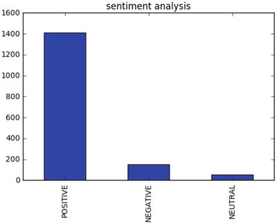
The procedure of discovering and classifying opinions expressed in a piece of text (like comments/feedback text) is called the sentiment analysis. The intended output of this analysis would be to determine whether the writer’s mindset toward a topic, product, service etc., is neutral, positive, or negative. See Listing 5-33.
Listing 5-33. Example code for sentiment analysis
from nltk.sentiment.vader import SentimentIntensityAnalyzerfrom nltk.sentiment.util import *data = pd.read_csv('Data/customer_review.csv')SIA = SentimentIntensityAnalyzer()data['polarity_score']=data.Review.apply(lambda x:SIA.polarity_scores(x)['compound'])data['neutral_score']=data.Review.apply(lambda x:SIA.polarity_scores(x)['neu'])data['negative_score']=data.Review.apply(lambda x:SIA.polarity_scores(x)['neg'])data['positive_score']=data.Review.apply(lambda x:SIA.polarity_scores(x)['pos'])data['sentiment']=''data.loc[data.polarity_score>0,'sentiment']='POSITIVE'data.loc[data.polarity_score==0,'sentiment']='NEUTRAL'data.loc[data.polarity_score<0,'sentiment']='NEGATIVE'data.head()data.sentiment.value_counts().plot(kind='bar',title="sentiment analysis")plt.show()#----output----ID Review polarity_score0 1 Excellent service my claim was dealt with very... 0.73461 2 Very sympathetically dealt within all aspects ... -0.81552 3 Having received yet another ludicrous quote fr... 0.97853 4 Very prompt and fair handling of claim. A mino... 0.14404 5 Very good and excellent value for money simple... 0.8610neutral_score negative_score positive_score sentiment0 0.618 0.000 0.382 POSITIVE1 0.680 0.320 0.000 NEGATIVE2 0.711 0.039 0.251 POSITIVE3 0.651 0.135 0.214 POSITIVE4 0.485 0.000 0.515 POSITIVE
Deep Natural Language Processing (DNLP )
First, let me clarify that DNLP is not to be mistaken for Deep Learning NLP. A technique such as topic modeling is generally known as shallow NLP where you try to extract knowledge from text through semantic or syntactic analysis approach, that is, try to form groups by retaining words that are similar and hold higher weight in a sentence/document. Shallow NLP is less noise than the n-grams; however the key drawback is that it does not specify the role of items in the sentence. In contrast, DNLP focuses on a semantic approach, that is, it detects relationships within the sentences, and further it can be represented or expressed as a complex construction of the form such as subject:predicate:object (known as triples or triplets) out of syntactically parsed sentences to retain the context. Sentences are made up of any combination of actor, action, object, and named entities (person, organizations, locations, dates, etc.). For example, consider the sentence "the flat tire was replaced by the driver." Here driver is the subject (actor), replaced is the predicate (action), and flat tire is the object (action). So the triples for would be driver:replaced:tire, which captures the context of the sentence. Note that triples are one of the forms widely used and you can form a similar complex structure based on the domain or problem at hand.
For demonstration I’ll use the sopex package , which uses Stanford Core NLP tree parser. See Listing 5-34.
Listing 5-34. Example code for Deep NLP
from chunker import PennTreebackChunkerfrom extractor import SOPExtractor# Initialize chunkerchunker = PennTreebackChunker()extractor = SOPExtractor(chunker)# function to extract triplesdef extract(sentence):sentence = sentence if sentence[-1] == '.' else sentence+'.'global extractorsop_triplet = extractor.extract(sentence)return sop_tripletsentences = ['The quick brown fox jumps over the lazy dog.','A rare black squirrel has become a regular visitor to a suburban garden','The driver did not change the flat tire',"The driver crashed the bike white bumper"]#Loop over sentence and extract triplesfor sentence in sentences:sop_triplet = extract(sentence)print sop_triplet.subject + ':' + sop_triplet.predicate + ':' + sop_triplet.object#----output----fox:jumps:dogsquirrel:become:visitordriver:change:tiredriver:crashed:bumper
Word2Vec
Tomas Mikolov’s lead team at Google created Word2Vec (word to vector) model in 2013, which uses documents to train a neural network model to maximize the conditional probability of a context given the word.
It utilizes two models: CBOW and skip-gram.
Continuous bag-of-words (CBOW) model predicts the current word from a window of surrounding context words or given a set of context words predict the missing word that is likely to appear in that context. CBOW is faster than skip-gram to train and gives better accuracy for frequently appearing words.
Continuous skip-gram model predicts the surrounding window of context words using the current word or given a single word, predict the probability of other words that are likely to appear near it in that context. Skip-gram is known to show good results for both frequent and rare words. Let’s look at an example sentence and create skip-gram for a window of 2 (refer to Figure 5-9). The word highlighted in yellow is the input word.
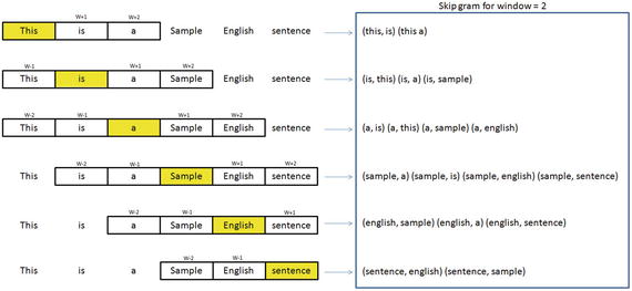
Figure 5-9. Skip-gram for window 2
You can download Google’s pre-trained model (from given link below) for word2vec, which includes a vocabulary of 3 million words/phrases taken from 100 billion words from a Google News dataset. See Listings 5-35 and 5-36.
URL: https://drive.google.com/file/d/0B7XkCwpI5KDYNlNUTTlSS21pQmM/edit
Listing 5-35. Example code for word2vec
import gensim# Load Google's pre-trained Word2Vec model.model = gensim.models.Word2Vec.load_word2vec_format('Data/GoogleNews-vectors-negative300.bin', binary=True)model.most_similar(positive=['woman', 'king'], negative=['man'], topn=5)#----output----[(u'queen', 0.7118192911148071),(u'monarch', 0.6189674139022827),(u'princess', 0.5902431607246399),(u'crown_prince', 0.5499460697174072),(u'prince', 0.5377321243286133)]model.most_similar(['girl', 'father'], ['boy'], topn=3)#----output----[(u'mother', 0.831214427947998),(u'daughter', 0.8000643253326416),(u'husband', 0.769158124923706)]model.doesnt_match("breakfast cereal dinner lunch".split())#----output----'cereal'You can train a word2vec model on your own data set. The key model parameters to be remembered are size, window, min_count and sg.size: The dimensionality of the vectors, the bigger size values require more training data, but can lead to more accurate modelssg = 0 for CBOW model and 1 for skip-gram modelmin_count: Ignore all words with total frequency lower than this.window: The maximum distance between the current and predicted word within a sentence
Listing 5-36. Example code for training word2vec on your own dataset
sentences = [['cigarette','smoking','is','injurious', 'to', 'health'],['cigarette','smoking','causes','cancer'],['cigarette','are','not','to','be','sold','to','kids']]# train word2vec on the two sentencesmodel = gensim.models.Word2Vec(sentences, min_count=1, sg=1, window = 3)model.most_similar(positive=['cigarette', 'smoking'], negative=['kids'], topn=1)#----output----[('injurious', 0.16142114996910095)]
Recommender Systems
Personalization of the user experience has been a high priority and has become the new mantra in the consumer-focused industry. You might have observed e-commerce companies casting personalized ads for you suggesting what to buy, which news to read, which video to watch, where/what to eat, and who you might be interested in networking (friends/professionals) on social media sites. Recommender systems are the core information filtering system designed to predict the user preference and help to recommend correct items to create a user-specific personalization experience. There are two types of recommendation systems: 1) content-based filtering and 2) collaborative filtering. See Figure 5-10.
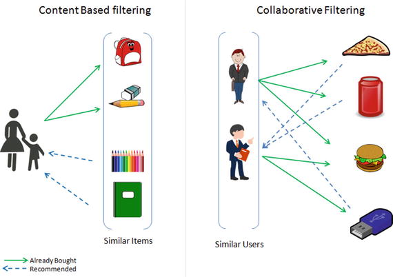
Figure 5-10. Recommender systems
Content-Based Filtering
This type of system focuses on the similarity attributes of the items to give you recommendations. This is best understood with an example, so if a user has purchased items of a particular category then other similar items from the same category are recommended to the user (refer to Figure 5-10).
An item-based similarity recommendation algorithm can be represented as shown here:
Collaborative Filtering (CF)
CF focuses on the similarity attribute of the users, that is,it finds people with similar tastes based on a similarity measure from the large group of users. There are two types of CF implementation in practice: memory-based and model-based.
The memory-based recommendation is mainly based on the similarity algorithm; the algorithm looks at items liked by similar people to create a ranked list of recommendations. You can then sort the ranked list to recommend the top n items to the user.
The user-based similarity recommendation algorithm can be represented as:
Let’s consider an example dataset of movie ratings (Figure 5-11) and apply item- and user-based recommendations to get a better understanding. See Listing 5-37.
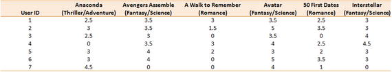
Figure 5-11. Movie rating sample dataset
Listing 5-37. Example code for recommender system
import numpy as npimport pandas as pddf = pd.read_csv('Data/movie_rating.csv')n_users = df.userID.unique().shape[0]n_items = df.itemID.unique().shape[0]print '\nNumber of users = ' + str(n_users) + ' | Number of movies = ' + str(n_items)#----output----Number of users = 7 | Number of movies = 6# Create user-item similarity matricesdf_matrix = np.zeros((n_users, n_items))for line in df.itertuples():df_matrix[line[1]-1, line[2]-1] = line[3]from sklearn.metrics.pairwise import pairwise_distancesuser_similarity = pairwise_distances(df_matrix, metric='cosine')item_similarity = pairwise_distances(df_matrix.T, metric='cosine')# Top 3 similar users for user id 7print "Similar users for user id 7: \n", pd.DataFrame(user_similarity).loc[6,pd.DataFrame(user_similarity).loc[6,:] > 0].sort_values(ascending=False)[0:3]#----output----Similar users for user id 7:3 8.0000000 6.0621785 5.873670# Top 3 similar items for item id 6print "Similar items for item id 6: \n", pd.DataFrame(item_similarity).loc[5,pd.DataFrame(item_similarity).loc[5,:] > 0].sort_values(ascending=False)[0:3]#----output----0 6.5574392 5.5226813 4.974937
Let’s build the user-based predict and item-based prediction for forumla as a function. Apply this function to predict ratings and use root mean squared error (RMSE) to evaluate the model performance.
See Listing 5-38.
Listing 5-38. Example code for recommender system & accuracy evaluation
# Function for item based rating predictiondef item_based_prediction(rating_matrix, similarity_matrix):return rating_matrix.dot(similarity_matrix) / np.array([np.abs(similarity_matrix).sum(axis=1)])# Function for user based rating predictiondef user_based_prediction(rating_matrix, similarity_matrix):mean_user_rating = rating_matrix.mean(axis=1)ratings_diff = (rating_matrix - mean_user_rating[:, np.newaxis])return mean_user_rating[:, np.newaxis] + similarity_matrix.dot(ratings_diff) / np.array([np.abs(similarity_matrix).sum(axis=1)]).Titem_based_prediction = item_based_prediction(df_matrix, item_similarity)user_based_prediction = user_based_prediction(df_matrix, user_similarity)# Calculate the RMSEfrom sklearn.metrics import mean_squared_errorfrom math import sqrtdef rmse(prediction, actual):prediction = prediction[actual.nonzero()].flatten()actual = actual[actual.nonzero()].flatten()return sqrt(mean_squared_error(prediction, actual))print 'User-based CF RMSE: ' + str(rmse(user_based_prediction, df_matrix))print 'Item-based CF RMSE: ' + str(rmse(item_based_prediction, df_matrix))#----output----User-based CF RMSE: 1.0705767849Item-based CF RMSE: 1.37392288971y_user_based = pd.DataFrame(user_based_prediction)# Predictions for movies that the user 6 hasn't rated yetpredictions = y_user_based.loc[6,pd.DataFrame(df_matrix).loc[6,:] == 0]top = predictions.sort_values(ascending=False).head(n=1)recommendations = pd.DataFrame(data=top)recommendations.columns = ['Predicted Rating']print recommendations#----output----Predicted Rating1 2.282415y_item_based = pd.DataFrame(item_based_prediction)# Predictions for movies that the user 6 hasn't rated yetpredictions = y_item_based.loc[6,pd.DataFrame(df_matrix).loc[6,:] == 0]top = predictions.sort_values(ascending=False).head(n=1)recommendations = pd.DataFrame(data=top)recommendations.columns = ['Predicted Rating']print recommendations#----output----Predicted Rating5 2.262497
Based on user based the recommended Intersellar is recommended (5th index). Based on item based the recommended movie is Avengers Assemble (index number 1).
Model-based CF is based on matrix factorization (MF) such as Singular Value Decomposition (SVD) and Non-nagative matrix factorization (NMF) etc. Let’s look how to implement using SVD.
See Listing 5-39.
Listing 5-39. Example code for recommender system using SVD
# calculate sparsity levelsparsity=round(1.0-len(df)/float(n_users*n_items),3)print 'The sparsity level of is ' + str(sparsity*100) + '%'import scipy.sparse as spfrom scipy.sparse.linalg import svds# Get SVD components from train matrix. Choose k.u, s, vt = svds(df_matrix, k = 5)s_diag_matrix=np.diag(s)X_pred = np.dot(np.dot(u, s_diag_matrix), vt)print 'User-based CF MSE: ' + str(rmse(X_pred, df_matrix))#----output----The sparsity level of is 0.0%User-based CF MSE: 0.015742898995
Note that, in our case the data set is small, hence sparsity level is 0%. I recommend you to try this method on the MovieLens 100k dataset which you can download from https://grouplens.org/datasets/movielens/100k/
Endnotes
In this step you have learned the fundamentals of the text mining process and different tools/techniques to extract text from various file formats. You also learned the basic text preprocessing steps to remove noise from data and different visualization techniques to better understand the corpus at hand. Then you learned various models that can be built to understand the relationship between the data and gain insight from it.
We also learned two important recommender system methods such as content-based filtering and collaborative filtering.