


In this chapter you will get a high-level overview of the Python language and its core philosophy, how to set up the Python development environment, and the key concepts around Python programming to get you started with basics. This chapter is an additional step or the prerequisite step for non-Python users. If you are already comfortable with Python, I would recommend that you quickly run through the contents to ensure you are aware of all of the key concepts.
The Best Things in Life Are Free
As the saying goes, “The best things in life are free!” Python is an open source, high-level, object-oriented, interpreted, and general-purpose dynamic programming language. It has a community-based development model. Its core design theory accentuates code readability, and its coding structure enables programmers to articulate computing concepts in fewer lines of code as compared to other high-level programming languages such as Java, C or C++.
The design philosophy of Python is well summarized by the document “The Zen of Python” (Python Enhancement Proposal, information entry number 20), which includes mottos such as the following:
Beautiful is better than ugly – be consistent.
Complex is better than complicated – use existing libraries.
Simple is better than complex – keep it simple and stupid (KISS).
Flat is better than nested – avoid nested ifs.
Explicit is better than implicit – be clear.
Sparse is better than dense – separate code into modules.
Readability counts – indenting for easy readability.
Special cases aren’t special enough to break the rules – everything is an object.
Errors should never pass silently – good exception handler.
Although practicality beats purity - if required, break the rules.
Unless explicitly silenced – error logging and traceability.
In ambiguity, refuse the temptation to guess – Python syntax is simpler; however, many times we might take a longer time to decipher it.
Although that way may not be obvious at first unless you’re Dutch – there is not only one of way of achieving something.
There should be preferably only one obvious way to do it – use existing libraries.
If the implementation is hard to explain, it’s a bad idea – if you can’t explain in simple terms then you don’t understand it well enough.
Now is better than never – there are quick/dirty ways to get the job done rather than trying too much to optimize.
Although never is often better than *right* now – although there is a quick/dirty way, don’t head in the path that will not allow a graceful way back.
Namespaces are one honking great idea, so let’s do more of those! – be specific.
If the implementation is easy to explain, it may be a good idea – simplicity.
The Rising Star
Python was officially born on February 20, 1991, with version number 0.9.0 and has taken a tremendous growth path to become the most popular language for the last 5 years in a row (2012 to 2016). Its application cuts across various areas such as website development, mobile apps development, scientific and numeric computing, desktop GUI, and complex software development. Even though Python is a more general-purpose programming and scripting language, it has been gaining popularity over the past 5 years among data scientists and Machine Learning engineers. See Figure 1-1.
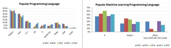
Figure 1-1. Popular Coding Language (Source: codeeval.com) and Popular Machine Learning Programming Language (Source:KDD poll)
There are well-designed development environments such as IPython Notebook and Spyder that allow for a quick introspection of the data and enable developing of machine learning models interactively.
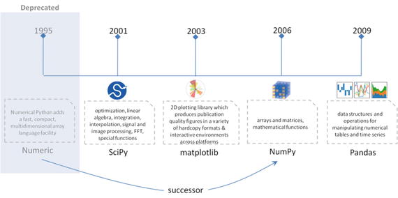
Powerful modules such as NumPy and Pandas exist for the efficient use of numeric data. Scientific computing is made easy with SciPy package. A number of primary machine learning algorithms have been efficiently implemented in scikit-learn (also known as sklearn). HadooPy, PySpark provides seamless work experience with big data technology stacks. Cython and Numba modules allow executing Python code in par with the speed of C code. Modules such as nosetest emphasize high-quality, continuous integration tests, and automatic deployment.
Combining all of the above has made many machine learning engineers embrace Python as the choice of language to explore data, identify patterns, and build and deploy models to the production environment. Most importantly the business-friendly licenses for various key Python packages are encouraging the collaboration of businesses and the open source community for the benefit of both worlds. Overall the Python programming ecosystem allows for quick results and happy programmers. We have been seeing the trend of developers being part of the open source community to contribute to the bug fixes and new algorithms for the use by the global community, at the same time protecting the core IP of the respective company they work for.
Python 2.7.x or Python 3.4.x?
Python 3.4.x is the latest version and comes with nicer, consistent functionalities! However, there is very limited third-party module support for it, and this will be the trend for at least a couple of more years. However, all major frameworks still run on version 2.7.x and are likely to continue to do so for a significant amount of time. Therefore, it is advised to start with Python 2, for the fact that it is the most widely used version for building machine learning systems as of today.
For an in-depth analysis of the differences between Python 2 vs. 3, you can refer to Wiki.python.org ( https://wiki.python.org/moin/Python2orPython3v ), which says that there are benefits to each.
I recommend Anaconda (Python distribution), which is BSD licensed and gives you permission to use it commercially and for redistribution. It has around 270 packages including the most important ones for most scientific applications, data analysis, and machine learning such as NumPy, SciPy, Pandas, IPython, matplotlib, and scikit-learn. It also provides a superior environment tool conda that allows you to easily switch between environments, even between Python 2 and 3 (if required). It is also updated very quickly as soon as a new version of a package is released and you can just use conda update <packagename> to update it.
You can download the latest version of Anaconda from their official website at https://www.continuum.io/downloads and follow the installation instructions.
Windows Installation
Download the installer depending on your system configuration (32 or 64 bit).
Double-click the .exe file to install Anaconda and follow the installation wizard on your screen.
OSX Installation
For Mac OS, you can install either through a graphical installer or from a command line.
Graphical Installer
Download the graphical installer.
Double-click the downloaded .pkg file and follow the installation wizard instructions on your screen.
Or
Command-Line Installer
Download the command-line installer.
In your terminal window type one of the below and follow the instructions: bash <Anaconda2-x.x.x-MacOSX-x86_64.sh>.
Linux Installation
Download the installer depending on your system configuration (32 or 64 bit).
In your terminal window type one of the below and follow the instructions: bash Anaconda2-x.x.x-Linux-x86_xx.sh.
Python from Official Website
For some reason if you don’t want to go with the Anaconda build pack, alternatively you can go to Python’s official website https://www.python.org/downloads/ and browse to the appropriate OS section and download the installer. Note that OSX and most of the Linux come with preinstalled Python so there is no need of additional configuring.
Setting up PATH for Windows: When you run the installer make sure to check the “Add Python to PATH option.” This will allow us to invoke the Python interpreter from any directory.
If you miss ticking “Add Python to PATH option,” follow these instructions:
Right-click on “My computer.”
Click “Properties.”
Click “Advanced system settings” in the side panel.
Click “Environment Variables.”
Click the “New” below system variables.
For the name, enter pythonexe (or anything you want).
For the value, enter the path to your Python (example: C:\Python32\).
Now edit the Path variable (in the system part) and add %pythonexe%; to the end of what’s already there.
Running Python
From the command line , type “Python” to open the interactive interpreter.
A Python script can be executed at the command line using the syntax here:
python <scriptname.py>
All the code used in this book are available as IPython Notebook (now known as the Jupyter Notebook), it is an interactive computational environment, in which you can combine code execution, rich text, mathematics, plots and rich media. You can launch the Jupyter Notebook by clicking on the icon installed by Anaconda in the start menu (Windows) or by typing ‘jupyter notebook’ in a terminal (cmd on Windows). Then browse for the relevant IPython Notebook file that you would like to paly with.
Note that the codes can break with change is package version, hence for reproducibility, I have shared my package version numbers, please refer Module_Versions IPython Notebook.
Key Concepts
There are a couple of fundamental concepts in Python, and understanding these are essential for a beginner to get started. A brief look at these concepts is to follow.
Python Identifiers
As the name suggests, identifiers help us to differentiate one entity from another. Python entities such as class, functions, and variables are called identifiers.
It can be a combination of upper- or lowercase letters (a to z or A to Z).
It can be any digits (0 to 9) or an underscore (_).
The general rules to be followed for writing identifiers in Python.
It cannot start with a digit. For example, 1variable is not valid, whereas variable1 is valid.
Python reserved keywords (refer to Table 1-1) cannot be used as identifiers.
Table 1-1. Python keywords
FALSE
Class
Finally
Is
return
None
Continue
For
Lambda
try
TRUE
Def
From
nonlocal
while
And
Del
Global
Not
with
As
Elif
If
Or
yield
Assert
Else
Import
Pass
Break
Except
In
Raise
Except for underscore (_), special symbols like !, @, #, $, % etc cannot be part of the identifiers.
Keywords
Table 1-1 lists the set of reserved words used in Python to define the syntax and structure of the language. Keywords are case sensitive, and all the keywords are in lowercase except True, False, and None.
My First Python Program
Launch the Python interactive on the command prompt, and then type the following text and press Enter.
>>> print "Hello, Python World!"If you are running Python 2.7.x from the Anaconda build pack, then you can also use the print statement with parentheses as in print (“Hello, Python World!”), which would produce the following result: Hello, Python World! See Figure 1-2.
Figure 1-2. Python vs. Others
Code Blocks (Indentation & Suites)
It is very important to understand how to write code blocks in Python. Let’s look at two key concepts around code blocks.
Indentation
One of the most unique features of Python is its use of indentation to mark blocks of code. Each line of code must be indented by the same amount to denote a block of code in Python. Unlike most other programming languages, indentation is not used to help make the code look pretty. Indentation is required to indicate which block of code a code or statement belongs to.
Suites
A collection of individual statements that makes a single code block are called suites in Python. A header line followed by a suite are required for compound or complex statements such as if, while, def, and class (we will understand each of these in details in the later sections). Header lines begin with a keyword, and terminate with a colon (:) and are followed by one or more lines that make up the suite. See Listings 1-1 and 1-2.
Listing 1-1. Example of correct indentation
# Correct indentationprint ("Programming is an important skill for Data Science")print ("Statistics is a important skill for Data Science")print ("Business domain knowledge is a important skill for Data Science")# Correct indentation, note that if statement here is an example of suitesx = 1if x == 1:print ('x has a value of 1')else:print ('x does NOT have a value of 1')
Listing 1-2. Example of incorrect indentation
# incorrect indentation, program will generate a syntax error# due to the space character inserted at the beginning of second lineprint ("Programming is an important skill for Data Science")print ("Statistics is a important skill for Data Science")print ("Business domain knowledge is a important skill for Data Science")3# incorrect indentation, program will generate a syntax error# due to the wrong indentation in the else statementx = 1if x == 1:print ('x has a value of 1')else:print ('x does NOT have a value of 1')
Basic Object Types
According to the Python data model reference, objects are Python’s notion for data. All data in a Python program is represented by objects or by relations between objects. In a sense, and in conformance to Von Neumann’s model of a “stored program computer,” code is also represented by objects.Every object has an identity, a type, and a value. See Table 1-2 and Listing 1-3.
Table 1-2. Python object types
Type | Examples | Comments |
|---|---|---|
None | None | # singleton null object |
Boolean | True, False | |
Integer | -1, 0, 1, sys.maxint | |
Long | 1L, 9787L | |
Float | 3.141592654 | |
inf, float(‘inf’) | # infinity | |
-inf | # neg infinity | |
nan, float(‘nan’) | # not a number | |
Complex | 2+8j | # note use of j |
String | ‘this is a string’, “also me” | # use single or double quote |
r‘raw string’, b‘ASCII string’ | ||
u‘unicode string’ | ||
Tuple | empty = () | # empty tuple |
(1, True, ‘ML’) | # immutable list or unalterable list | |
List | empty = [] | empty list |
[1, True, ‘ML’] | # mutable list or alterable list | |
Set | empty = set() | # empty set |
set(1, True, ‘ML’) | # mutable or alterable | |
dictionary | empty = {} {‘1’:‘A’, ‘2’:‘AA’, True = 1, False = 0} | # mutable object or alterable object |
File | f = open(‘filename’, ‘rb’) |
Listing 1-3. Code For Basic Object Types
none = None # singleton null objectboolean = bool(True)integer = 1Long = 3.14# floatFloat = 3.14Float_inf = float('inf')Float_nan = float('nan')# complex object type, note the usage of letter jComplex = 2+8j# string can be enclosed in single or double quotestring = 'this is a string'me_also_string = "also me"List = [1, True, 'ML'] # Values can be changedTuple = (1, True, 'ML') # Values can not be changedSet = set([1,2,2,2,3,4,5,5]) # Duplicates will not be stored# Use a dictionary when you have a set of unique keys that map to valuesDictionary = {'a':'A', 2:'AA', True:1, False:0}# lets print the object type and the valueprint type(none), noneprint type(boolean), booleanprint type(integer), integerprint type(Long), Longprint type(Float), Floatprint type(Float_inf), Float_infprint type(Float_nan), Float_nanprint type(Complex), Complexprint type(string), stringprint type(me_also_string), me_also_stringprint type(Tuple), Tupleprint type(List), Listprint type(Set), Setprint type(Dictionary), Dictionary----- output ------<type 'NoneType'> None<type 'bool'> True<type 'int'> 1<type 'float'> 3.14<type 'float'> 3.14<type 'float'> inf<type 'float'> nan<type 'complex'> (2+8j)<type 'str'> this is a string<type 'str'> also me<type 'tuple'> (1, True, 'ML')<type 'list'> [1, True, 'ML']<type 'set'> set([1, 2, 3, 4, 5])<type 'dict'> {'a': 'A', True: 1, 2: 'AA', False: 0}
When to Use List vs. Tuples vs. Set vs. Dictionary
List: Use when you need an ordered sequence of homogenous collections, whose values can be changed later in the program.
Tuple: Use when you need an ordered sequence of heterogeneous collections whose values need not be changed later in the program.
Set: It is ideal for use when you don’t have to store duplicates and you are not concerned about the order or the items. You just want to know whether a particular value already exists or not.
Dictionary: It is ideal for use when you need to relate values with keys, in order to look them up efficiently using a key.
Comments in Python
Single line comment: Any characters followed by the # (hash) and up to the end of the line are considered a part of the comment and the Python interpreter ignores them.
Multiline comments : Any characters between the strings """ (referred as multiline string), that is, one at the beginning and end of your comments will be ignored by the Python interpreter. See Listing 1-4.
Listing 1-4. Example code for comments
# This is a single line comment in Pythonprint "Hello Python World" # This is also a single line comment in Python""" This is an example of a multi linecomment that runs into multiple lines.Everything that is in between is considered as comments"""
Multiline Statement
Python’s oblique line continuation inside parentheses, brackets, and braces is the favorite way of casing longer lines. Using backslash to indicate line continuation makes readability better; however if needed you can add an extra pair of parentheses around the expression. It is important to correctly indent the continued line of your code. Note that the preferred place to break around the binary operator is after the operator, and not before it. See Listing 1-5.
Listing 1-5. Example code for multiline statements
# Example of implicit line continuationx = ('1' + '2' +'3' + '4')# Example of explicit line continuationy = '1' + '2' + \'11' + '12'weekdays = ['Monday', 'Tuesday', 'Wednesday','Thursday', 'Friday']weekend = {'Saturday','Sunday'}print ('x has a value of', x)print ('y has a value of', y)print daysprint weekend------ output -------('x has a value of', '1234')('y has a value of', '1234')['Monday', 'Tuesday', 'Wednesday', 'Thursday', 'Friday']set(['Sunday', 'Saturday'])
Multiple Statements on a Single Line
Python also allows multiple statements on a single line through usage of the semicolon (;), given that the statement does not start a new code block. See Listing 1-6.
Listing 1-6. Code example for multistatements on a single line
import os; x = 'Hello'; print xBasic Operators
In Python, operators are the special symbols that can manipulate the value of operands. For example, let’s consider the expression 1 + 2 = 3. Here, 1 and 2 are called operands, which are the value on which operators operate and the symbol + is called an operator.
Python language supports the following types of operators .
Arithmetic Operators
Comparison or Relational Operators
Assignment Operators
Bitwise Operators
Logical Operators
Membership Operators
Identity Operators
Let’s learn all operators through examples one by one.
Arithmetic Operators
Arithmetic operators are useful for performing mathematical operations on numbers such as addition, subtraction, multiplication, division, etc. See Table 1-3 and then Listing 1-7.
Table 1-3. Arithmetic operators
Operator | Description | Example |
|---|---|---|
+ | Addition | x + y = 30 |
- | Subtraction | x – y = -10 |
* | Multiplication | x * y = 200 |
/ | Division | y / x = 2 |
% | Modulus | y % x = 0 |
** Exponent | Exponentiation | x**b =10 to the power 20 |
// | Floor Division – Integer division rounded toward minus infinity | 9//2 = 4 and 9.0//2.0 = 4.0, -11//3 = -4, -11.0/ |
Listing 1-7. Example code for arithmetic operators
# Variable x holds 10 and variable y holds 5x = 10y = 5# Additionprint "Addition, x(10) + y(5) = ", x + y# Subtractionprint "Subtraction, x(10) - y(5) = ", x - y# Multiplicationprint "Multiplication, x(10) * y(5) = ", x * y# Divisionprint "Division, x(10) / y(5) = ",x / y# Modulusprint "Modulus, x(10) % y(5) = ", x % y# Exponentprint "Exponent, x(10)**y(5) = ", x**y# Integer division rounded towards minus infinityprint "Floor Division, x(10)//y(5) = ", x//y-------- output --------Addition, x(10) + y(5) = 15Subtraction, x(10) - y(5) = 5Multiplication, x(10) * y(5) = 50Divions, x(10) / y(5) = 2Modulus, x(10) % y(5) = 0Exponent, x(10)**y(5) = 100000Floor Division, x(10)//y(5) = 2
Comparison or Relational Operators
As the name suggests the comparison or relational operators are useful to compare values. It would return True or False as a result for a given condition. See Table 1-4 and Listing 1-8.
Table 1-4. Comparison or Relational operators
Operator | Description | Example |
|---|---|---|
== | The condition becomes True, if the values of two operands are equal. | (x == y) is not true. |
!= | The condition becomes True, if the values of two operands are not equal. | |
<> | The condition becomes True, if values of two operands are not equal. | (x<>y) is true. This is similar to != operator. |
> | The condition becomes True, if the value of left operand is greater than the value of right operand. | (x>y) is not true. |
< | The condition becomes True, if the value of left operand is less than the value of right operand. | (x<y) is true. |
>= | The condition becomes True, if the value of left operand is greater than or equal to the value of right operand. | (x>= y) is not true. |
<= | The condition becomes True, if the value of left operand is less than or equal to the value of right operand. | (x<= y) is true. |
Listing 1-8. Example code for comparision/relational operators
# Variable x holds 10 and variable y holds 5x = 10y = 5# Equal check operationprint "Equal check, x(10) == y(5) ", x == y# Not Equal check operationprint "Not Equal check, x(10) != y(5) ", x != y# Not Equal check operationprint "Not Equal check, x(10) <>y(5) ", x<>y# Less than check operationprint "Less than check, x(10) <y(5) ", x<y# Greater check operationprint "Greater than check, x(10) >y(5) ", x>y# Less than or equal check operationprint "Less than or equal to check, x(10) <= y(5) ", x<= y# Greater than or equal to check operationprint "Greater than or equal to check, x(10) >= y(5) ", x>= y-------- output --------Equal check, x(10) == y(5) FalseNot Equal check, x(10) != y(5) TrueNot Equal check, x(10) <>y(5) TrueLess than check, x(10) <y(5) FalseGreater than check, x(10) >y(5) TrueLess than or equal to check, x(10) <= y(5) FalseGreater than or equal to check, x(10) >= y(5) True
Assignment Operators
In Python, assignment operators are used for assigning values to variables. For example, consider x = 5; it is a simple assignment operator that assigns the numeric value 5, which is on the right side of the operator onto the variable x on the left side of operator. There is a range of compound operators in Python like x += 5 that add to the variable and later assign the same. It is as good as x = x + 5. See Table 1-5 and Listing 1-9.
Table 1-5. Assignment operators
Operator | Description | Example |
|---|---|---|
= | Assigns values from right side operands to left side operand. | z = x + y assigns value of x + y into z |
+= Add AND | It adds right operand to the left operand and assigns the result to left operand. | z += x is equivalent to z = z + x |
-= Subtract AND | It subtracts right operand from the left operand and assigns the result to left operand. | z -= x is equivalent to z = z - x |
*= Multiply AND | It multiplies right operand with the left operand and assigns the result to left operand. | z *= x is equivalent to z = z * x |
/= Divide AND | It divides left operand with the right operand and assigns the result to left operand. | z /= x is equivalent to z = z/ xz /= x is equivalent to z = z / x |
%= Modulus AND | It takes modulus using two operands and assigns the result to left operand. | z %= x is equivalent to z = z % x |
**= Exponent AND | Performs exponential (power) calculation on operators and assigns value to the left operand. | z **= x is equivalent to z = z ** x |
//= Floor Division | It performs floor division on operators and assigns value to the left operand. | z //= x is equivalent to z = z// x |
Listing 1-9. Example code for assignment operators
# Variable x holds 10 and variable y holds 5x = 5y = 10x += yprint "Value of a post x+=y is ", xx *= yprint "Value of a post x*=y is ", xx /= yprint "Value of a post x/=y is ", xx %= yprint "Value of a post x%=y is ", xx **= yprint "Value of x post x**=y is ", xx //= yprint "Value of a post x//=y is ", x-------- output --------Value of a post x+=y is 15Value of a post x*=y is 150Value of a post x/=y is 15Value of a post x%=y is 5Value of a post x**=y is 9765625Value of a post x//=y is 976562
Bitwise Operators
As you might be aware, everything in a computer is represented by bits, that is, a series of 0’s (zero) and 1’s (one). Bitwise operators enable us to directly operate or manipulate bits. Let’s understand the basic bitwise operations. One of the key usages of bitwise operators is for parsing hexadecimal colors.
Bitwise operators are known to be confusing for newbies to Python programming, so don’t be anxious if you don’t understand usability at first. The fact is that you aren’t really going to see bitwise operators in your everyday machine learning programming. However, it is good to be aware about these operators.
For example let’s assume that x = 10 (in binary 0000 1010) and y = 4 (in binary 0000 0100). See Table 1-6 and Listing 1-10.
Table 1-6. Bitwise operators
Operator | Description | Example |
|---|---|---|
& Binary AND | This operator copies a bit to the result if it exists in both operands. | (x&y) (means 0000 0000) |
| Binary OR | This operator copies a bit if it exists in either operand. | (x | y) = 14 (means 0000 1110) |
^ Binary XOR | This operator copies the bit if it is set in one operand but not both. | (x ^ y) = 14 (means 0000 1110) |
∼ Binary Ones Complement | This operator is unary and has the effect of ‘flipping’ bits. | (∼x ) = -11 (means 1111 0101) |
<< Binary Left Shift | The left operands value is moved left by the number of bits specified by the right operand. | x<< 2= 42 (means 0010 1000) |
>> Binary Right Shift | The left operands value is moved right by the number of bits specified by the right operand. | x>> 2 = 2 (means 0000 0010) |
Listing 1-10. Example code for bitwise operators
# Basic six bitwise operations# Let x = 10 (in binary0000 1010) and y = 4 (in binary0000 0100)x = 10y = 4print x >> y # Right Shiftprint x << y # Left Shiftprint x & y # Bitwise ANDprint x | y # Bitwise ORprint x ^ y # Bitwise XORprint ∼x # Bitwise NOT-------- output --------016001414-11
Logical Operators
The AND, OR, NOT operators are called logical operators. These are useful to check two variables against given condition and the result will be True or False appropriately. See Table 1-7 and Listing 1-11.
Table 1-7. Logical operators
Operator | Description | Example |
|---|---|---|
and Logical AND | If both the operands are true then condition becomes true. | (var1 and var2) is true. |
or Logical OR | If any of the two operands are non-zero then condition becomes true. | (var1 or var2) is true. |
not Logical NOT | Used to reverse the logical state of its operand. | Not (var1 and var2) is false. |
Listing 1-11. Example code for logical operators
var1 = Truevar2 = Falseprint('var1 and var2 is',var1and var2)print('var1 or var2 is',var1 or var2)print('not var1 is',not var1)-------- output --------('var1 and var2 is', False)('var1 or var2 is', True)('not var1 is', False)
Membership Operators
Membership operators are useful to test if a value is found in a sequence, that is, string, list, tuple, set, or dictionary. There are two membership operators in Python, ‘in’ and ‘not in’. Note that we can only test for presence of key (and not the value) in case of a dictionary. See Table 1-8 and Listing 1-12.
Table 1-8. Membership operators
Operator | Description | Example |
|---|---|---|
In | Results to True if a value is in the specified sequence and False otherwise. | var1 in var2 |
not in | Results to True, if a value is not in the specified sequence and False otherwise. | var1 not in var2 |
Listing 1-12. Example code for membership operators
var1 = 'Hello world' # stringvar1 = {1:'a',2:'b'}# dictionaryprint('H' in var1)print('hello' not in var2)print(1 in var2)print('a' in var2)-------- output --------TrueTrueTrueFalse
Identity Operators
Identity operators are useful to test if two variables are present on the same part of the memory. There are two identity operators in Python, ‘is’ and ‘is not’. Note that two variables having equal values do not imply they are identical. See Table 1-9 and Listing 1-13.
Table 1-9. Identity operators
Operator | Description | Example |
|---|---|---|
Is | Results to True, if the variables on either side of the operator point to the same object and False otherwise. | var1 is var2 |
is not | Results to False, if the variables on either side of the operator point to the same object and True otherwise. | Var1 is not var2 |
Listing 1-13. Example code for identity operators
var1 = 5var1 = 5var2 = 'Hello'var2 = 'Hello'var3 = [1,2,3]var3 = [1,2,3]print(var1 is not var1)print(var2 is var2)print(var3 is var3)-------- output --------FalseTrueFalse
Control Structure
A control structure is the fundamental choice or decision-making process in programming. It is a chunk of code that analyzes values of variables and decides a direction to go based on a given condition. In Python there are mainly two types of control structures: (1) selection and (2) iteration.
Selection
Selection statements allow programmers to check a condition and based on the result will perform different actions. There are two versions of this useful construct: (1) if and (2) if…else. See Listings 1-14, 1-15, and 1-16.
Listing 1-14. Example code for a simple ‘if’ statement
var = -1if var < 0:print varprint("the value of var is negative")# If there is only a signle cluse then it may go on the same line as the header statementif ( var == -1 ) : print "the value of var is negative"
Listing 1-15. Example code for ‘if else’ statement
var = 1if var < 0:print "the value of var is negative"print varelse:print "the value of var is positive"print var
Listing 1-16. Example code for nested if else statements
Score = 95if score >= 99:print('A')elif score >=75:print('B')elif score >= 60:print('C')elif score >= 35:print('D')else:print('F')
Iteration
A loop control statement enables us to execute a single or a set of programming statements multiple times until a given condition is satisfied. Python provides two essential looping statements: (1) for (2) while statement.
For loop: It allows us to execute code block for a specific number of times or against a specific condition until it is satisfied. See Listing 1-17.
Listing 1-17. Example codes for a ‘for loop’ statement
# First Exampleprint "First Example"for item in [1,2,3,4,5]:print 'item :', item# Second Exampleprint "Second Example"letters = ['A', 'B', 'C']for letter in letters:print ' First loop letter :', letter# Third Example - Iterating by sequency indexprint "Third Example"for index in range(len(letters)):print 'First loop letter :', letters[index]# Fourth Example - Using else statementprint "Fourth Example"for item in [1,2,3,4,5]:print 'item :', itemelse:print 'looping over item complete!'----- output ------First Exampleitem : 1item : 2item : 3item : 4item : 5Second ExampleFirst loop letter : AFirst loop letter : BFirst loop letter : CThird ExampleFirst loop letter : AFirst loop letter : BFirst loop letter : CFourth Exampleitem : 1item : 2item : 3item : 4item : 5looping over item complete!
While loop: The while statement repeats a set of code until the condition is true. See Listing 1-18.
Listing 1-18. Example code for while loop statement
count = 0while (count <3):print 'The count is:', countcount = count + 1
Caution
If a condition never becomes FALSE, a loop becomes an infinite loop.
An else statement can be used with a while loop and the else will be executed when the condition becomes false. See Listing 1-19.
Listing 1-19. example code for a ‘while with a else’ statement
count = 0while count <3:print count, " is less than 5"count = count + 1else:print count, " is not less than 5"
Lists
Python’s lists are the most flexible data type. It can be created by writing a list of comma-separated values between square brackets. Note that that the items in the list need not be of the same data type. See Table 1-10; and Listings 1-20, 1-21, 1-22, 1-23, and 1-24.
Table 1-10. Python list operations
Description | Python Expression | Example | Results |
|---|---|---|---|
Creating a list of items | [item1, item2, …] | list = [‘a’,‘b’,‘c’,‘d’] | [‘a’,‘b’,‘c’,‘d’] |
Accessing items in list | list[index] | list = [‘a’,‘b’,‘c’,‘d’] list[2] | c |
Length | len(list) | len([1, 2, 3]) | 3 |
Concatenation | list_1 + list_2 | [1, 2, 3] + [4, 5, 6] | [1, 2, 3, 4, 5, 6] |
Repetition | list * int | [‘Hello’] * 3 | [‘Hello’, ‘Hello’, ‘Hello’] |
Membership | item in list | 3 in [1, 2, 3] | TRUE |
Iteration | for x in list: print x | for x in [1, 2, 3]: print x, | 1 2 3 |
Count from the right | list[-index] | list = [1,2,3]; list[-2] | 2 |
Slicing fetches sections | list[index:] | list = [1,2,3]; list[1:] | [2,3] |
Comparing lists | cmp(list_1, list_2) | print cmp([1,2,3,4], [5,6,7]); print cmp([1,2,3], [5,6,7,8]) | 1 -1 |
Return max item | max(list) | max([1,2,3,4,5]) | 5 |
Return min item | min(list) | max([1,2,3,4,5]) | 1 |
Append object to list | list.append(obj) | [1,2,3,4].append(5) | [1,2,3,4,5] |
Count item occurrence | list.count(obj) | [1,1,2,3,4].count(1) | 2 |
Append content of sequence to list | list.extend(seq) | [‘a’, 1].extend([‘b’, 2]) | [‘a’, 1, ‘b’, 2] |
Return the first index position of item | list.index(obj) | [‘a’, ‘b’,‘c’,1,2,3].index(‘c’) | 2 |
Insert object to list at a desired index | list.insert(index, obj) | [‘a’, ‘b’,‘c’,1,2,3].insert(4, ‘d’) | [‘a’, ‘b’,‘c’,‘d’, 1,2,3] |
Remove and return last object from list | list.pop(obj=list[-1]) | [‘a’, ‘b’,‘c’,1,2,3].pop() [‘a’, ‘b’,‘c’,1,2,3].pop(2) | 3 c |
Remove object from list | list.remove(obj) | [‘a’, ‘b’,‘c’,1,2,3].remove(‘c’) | [‘a’, ‘b’, 1,2,3] |
Reverse objects of list in place | list.reverse() | [‘a’, ‘b’,‘c’,1,2,3].reverse() | [3,2,1,‘c’,‘b’,‘a’] |
Sort objects of list | list.sort() | [‘a’, ‘b’,‘c’,1,2,3].sort() [‘a’, ‘b’,‘c’,1,2,3].sort(reverse = True) | [1,2,3,‘a’, ‘b’,‘c’] [‘c’,‘b’,‘a’,3,2,1] |
Listing 1-20. Example code for accessing lists
# Create listslist_1 = ['Statistics', 'Programming', 2016, 2017, 2018];list_2 = ['a', 'b', 1, 2, 3, 4, 5, 6, 7 ];# Accessing values in listsprint "list_1[0]: ", list_1[0]print "list2_[1:5]: ", list_2[1:5]---- output ----list_1[0]: Statisticslist2_[1:5]: ['b', 1, 2, 3]
Listing 1-21. Example code for adding new values to lists
print "list_1 values: ", list_1# Adding new value to listlist_1.append(2019)print "list_1 values post append: ", list_1---- output ----list_1 values: ['c', 'b', 'a', 3, 2, 1]list_1 values post append: ['c', 'b', 'a', 3, 2, 1, 2019]
Listing 1-22. Example code for updating existing values of lists
print "Values of list_1: ", list_1# Updating existing value of listprint "Index 2 value : ", list_1[2]list_1[2] = 2015;print "Index 2's new value : ", list_1[2]---- output ----Values of list_1: ['c', 'b', 'a', 3, 2, 1, 2019]Index 2 value : aIndex 2's new value : 2015
Listing 1-23. Example code for deleting a list element
Print "list_1 values: ", list_1# Deleting list elementdel list_1[5];print "After deleting value at index 2 : ", list_1---- output ----list_1 values: ['c', 'b', 2015, 3, 2, 1, 2019]After deleting value at index 2 : ['c', 'b', 2015, 3, 2, 2019]
Listing 1-24. Example code for basic operations on lists
print "Length: ", len(list_1)print "Concatenation: ", [1,2,3] + [4, 5, 6]print "Repetition :", ['Hello'] * 4print "Membership :", 3 in [1,2,3]print "Iteration :"for x in [1,2,3]: print x# Negative sign will count from the rightprint "slicing :", list_1[-2]# If you dont specify the end explicitly, all elements from the specified start index will be printedprint "slicing range: ", list_1[1:]# Comparing elements of listsprint "Compare two lists: ", cmp([1,2,3, 4], [1,2,3])print "Max of list: ", max([1,2,3,4,5])print "Min of list: ", min([1,2,3,4,5])print "Count number of 1 in list: ", [1,1,2,3,4,5,].count(1)list_1.extend(list_2)print "Extended :", list_1print "Index for Programming : ", list_1.index( 'Programming')print list_1print "pop last item in list: ", list_1.pop()print "pop the item with index 2: ", list_1.pop(2)list_1.remove('b')print "removed b from list: ", list_1list_1.reverse()print "Reverse: ", list_1list_1 = ['a', 'b','c',1,2,3]list_1.sort()print "Sort ascending: ", list_1list_1.sort(reverse = True)print "Sort descending: ", list_1---- output ----Length: 5Concatenation: [1, 2, 3, 4, 5, 6]Repetition : ['Hello', 'Hello', 'Hello', 'Hello']Membership : TrueIteration :123slicing : 2017slicing range: ['Programming', 2015, 2017, 2018]Compare two lists: 1Max of list: 5Min of list: 1Count number of 1 in list: 2Extended : ['Statistics', 'Programming', 2015, 2017, 2018, 'a', 'b', 1, 2, 3, 4, 5, 6, 7]Index for Programming : 1['Statistics', 'Programming', 2015, 2017, 2018, 'a', 'b', 1, 2, 3, 4, 5, 6, 7]pop last item in list: 7pop the item with index 2: 2015removed b from list: ['Statistics', 'Programming', 2017, 2018, 'a', 1, 2, 3, 4, 5, 6]Reverse: [6, 5, 4, 3, 2, 1, 'a', 2018, 2017, 'Programming', 'Statistics']Sort ascending: [1, 2, 3, 'a', 'b', 'c']Sort descending: ['c', 'b', 'a', 3, 2, 1]
Tuple
A Python tuple is a sequences or series of immutable Python objects very much similar to the lists. However there exist some essential differences between lists and tuples, which are the following. See also Table 1-11; and Listings 1-25, 1-26, 1-27, and 1-28.
Unlike list, the objects of tuples cannot be changed.
Tuples are defined by using parentheses, but lists are defined by square brackets.
Table 1-11. Python Tuple operations
Description | Python Expression | Example | Results |
|---|---|---|---|
Creating a tuple | (item1, item2, …) () # empty tuple (item1,) # Tuple with one item, note comma is required | tuple = (‘a’,‘b’,‘c’,‘d’,1,2,3) tuple = () tuple = (1,) | (‘a’,‘b’,‘c’,‘d’,1,2,3) () 1 |
Accessing items in tuple | tuple[index] tuple[start_index:end_index] | tuple = (‘a’,‘b’,‘c’,‘d’,1,2,3) tuple[2] tuple[0:2] | c a, b, c |
Deleting a tuple | del tuple_name | del tuple | |
Length | len(tuple) | len((1, 2, 3)) | 3 |
Concatenation | tuple_1 + tuple_2 | (1, 2, 3) + (4, 5, 6) | (1, 2, 3, 4, 5, 6) |
Repetition | tuple * int | (‘Hello’,) * 4 | (‘Hello’, ‘Hello’, ‘Hello’, ‘Hello’) |
Membership | item in tuple | 3 in (1, 2, 3) | TRUE |
Iteration | for x in tuple: print x | for x in (1, 2, 3): print x | 1 2 3 |
Count from the right | tuple[-index] | tuple = (1,2,3); list[-2] | 2 |
Slicing fetches sections | tuple[index:] | tuple = (1,2,3); list[1:] | (2,3) |
Comparing lists | cmp(tuple_1, tuple_2) | print cmp((1,2,3,4), (5,6,7)); print cmp((1,2,3), (5,6,7,8)) | 1 -1 |
Return max item | max(tuple) | max((1,2,3,4,5)) | 5 |
Return min item | min(tuple) | max((1,2,3,4,5)) | 1 |
Convert a list to tuple | tuple(seq) | tuple([1,2,3,4]) | (1,2,3,4,5) |
Listing 1-25. Example code for creating tuple
# Creating a tupleTuple = ()print "Empty Tuple: ", TupleTuple = (1,)print "Tuple with single item: ", TupleTuple = ('a','b','c','d',1,2,3)print "Sample Tuple :", Tuple---- output ----Empty Tuple: ()Tuple with single item: (1,)Sample Tuple : ('a', 'b', 'c', 'd', 1, 2, 3)
Listing 1-26. Example code for accessing tuple
# Accessing items in tupleTuple = ('a', 'b', 'c', 'd', 1, 2, 3)print "3rd item of Tuple:", Tuple[2]print "First 3 items of Tuple", Tuple[0:2]---- output ----3rd item of Tuple: cFirst 3 items of Tuple ('a', 'b')
Listing 1-27. Example code for deleting tuple
# Deleting tupleprint "Sample Tuple: ", Tupledel Tupleprint Tuple # Will throw an error message as the tuple does not exist---- output ----Sample Tuple: ('a', 'b', 'c', 'd', 1, 2, 3)---------------------------------------------------------------------------NameError Traceback (most recent call last)<ipython-input-35-6a0deb3cfbcf> in <module>()3 print "Sample Tuple: ", Tuple4 del Tuple----> 5 print Tuple # Will throw an error message as the tuple does not existNameError: name 'Tuple' is not defined
Listing 1-28. Example code for basic operations on tupe (not exhaustive)
# Basic Tuple operationsTuple = ('a','b','c','d',1,2,3)print "Length of Tuple: ", len(Tuple)Tuple_Concat = Tuple + (7,8,9)print "Concatinated Tuple: ", Tuple_Concatprint "Repetition: ", (1, 'a',2, 'b') * 3print "Membership check: ", 3 in (1,2,3)# Iterationfor x in (1, 2, 3): print xprint "Negative sign will retrieve item from right: ", Tuple_Concat[-2]print "Sliced Tuple [2:] ", Tuple_Concat[2:]# Comparing two tuplesprint "Comparing tuples (1,2,3) and (1,2,3,4): ", cmp((1,2,3), (1,2,3,4))print "Comparing tuples (1,2,3,4) and (1,2,3): ", cmp((1,2,3,4), (1,2,3))# Find maxprint "Max of the Tuple (1,2,3,4,5,6,7,8,9,10): ", max((1,2,3,4,5,6,7,8,9,10))print "Min of the Tuple (1,2,3,4,5,6,7,8,9,10): ", min((1,2,3,4,5,6,7,8,9,10))print "List [1,2,3,4] converted to tuple: ", type(tuple([1,2,3,4]))---- output ----Length of Tuple: 7Concatinated Tuple: ('a', 'b', 'c', 'd', 1, 2, 3, 7, 8, 9)Repetition: (1, 'a', 2, 'b', 1, 'a', 2, 'b', 1, 'a', 2, 'b')Membership check: True123Negative sign will retrieve item from right: 8Sliced Tuple [2:] ('c', 'd', 1, 2, 3, 7, 8, 9)Comparing tuples (1,2,3) and (1,2,3,4): -1Comparing tuples (1,2,3,4) and (1,2,3): 1Max of the Tuple (1,2,3,4,5,6,7,8,9,10): 10Min of the Tuple (1,2,3,4,5,6,7,8,9,10): 1List [1,2,3,4] converted to tuple: <type 'tuple'>
Sets
As the name implies, sets are the implementations of mathematical sets. Three key characteristic of set are the following.
The collection of items is unordered.
No duplicate items will be stored, which means that each item is unique.
Sets are mutable, which means the items of it can be changed.
An item can be added or removed from sets. Mathematical set operations such as union, intersection, etc., can be performed on Python sets. See Table 1-12 and Listing 1-29.
Table 1-12. Python set operations
Description | Python Expression | Example | Results |
|---|---|---|---|
Creating a set. | set{item1, item2, …} set() # empty set | languages = set([‘Python’, ‘R’, ‘SAS’, ‘Julia’]) | set([‘SAS’, ‘Python’, ‘R’, ‘Julia’]) |
Add an item/element to a set. | add() | languages.add(‘SPSS’) | set([‘SAS’, ‘SPSS’, ‘Python’, ‘R’, ‘Julia’]) |
Remove all items/elements from a set. | clear() | languages.clear() | set([]) |
Return a copy of a set. | copy() | lang = languages.copy() print lang | set([‘SAS’, ‘SPSS’, ‘Python’, ‘R’, ‘Julia’]) |
Remove an item/element from set if it is a member. (Do nothing if the element is not in set). | discard() | languages = set([‘C’, ‘Java’, ‘Python’, ‘Data Science’, ‘Julia’, ‘SPSS’, ‘AI’, ‘R’, ‘SAS’, ‘Machine Learning’]) languages.discard(‘AI’) | set([‘C’, ‘Java’, ‘Python’, ‘Data Science’, ‘Julia’, ‘SPSS’, ‘R’, ‘SAS’, ‘Machine Learning’]) |
Remove an item/element from a set. If the element is not a member, raise a KeyError. | remove() | languages = set([‘C’, ‘Java’, ‘Python’, ‘Data Science’, ‘Julia’, ‘SPSS’, ‘AI’, ‘R’, ‘SAS’, ‘Machine Learning’]) languages.remove(‘AI’) | set([‘C’, ‘Java’, ‘Python’, ‘Data Science’, ‘Julia’, ‘SPSS’, ‘R’, ‘SAS’, ‘Machine Learning’]) |
Remove and return an arbitrary set element. RaiseKeyError if the set is empty. | pop() | languages = set([‘C’, ‘Java’, ‘Python’, ‘Data Science’, ‘Julia’, ‘SPSS’, ‘AI’, ‘R’, ‘SAS’, ‘Machine Learning’]) print “Removed:”, (languages.pop()) print(languages) | Removed: C set([‘Java’, ‘Python’, ‘Data Science’, ‘Julia’, ‘SPSS’, ‘R’, ‘SAS’, ‘Machine Learning’]) |
Return the difference of two or more sets as a new set. | difference() | # initialize A and B A = {1, 2, 3, 4, 5} B = {4, 5, 6, 7, 8} A.difference(B) | {1, 2, 3} |
Remove all item/elements of another set from this set. | difference_update() | # initialize A and B A = {1, 2, 3, 4, 5} B = {4, 5, 6, 7, 8} A.difference_update(B) print A | set([1, 2, 3]) |
Return the intersection of two sets as a new set. | intersection() | # initialize A and B A = {1, 2, 3, 4, 5} B = {4, 5, 6, 7, 8} A.intersection(B) | {4, 5} |
Update the set with the intersection of itself and another. | intersection_update() | # initialize A and B A = {1, 2, 3, 4, 5} B = {4, 5, 6, 7, 8} A.intersection_update B print A | set([4, 5]) |
Return True if two sets have a null intersection. | isdisjoint() | # initialize A and B A = {1, 2, 3, 4, 5} B = {4, 5, 6, 7, 8} A.isdisjoint(B) | FALSE |
Return True if another set contains this set. | issubset() | # initialize A and B A = {1, 2, 3, 4, 5} B = {4, 5, 6, 7, 8} print A.issubset(B) | FALSE |
Return True if this set contains another set. | issuperset() | # initialize A and B A = {1, 2, 3, 4, 5} B = {4, 5, 6, 7, 8} print A.issuperset(B) | FALSE |
Return the symmetric difference of two sets as a new set. | symmetric_difference() | # initialize A and B A = {1, 2, 3, 4, 5} B = {4, 5, 6, 7, 8} A. symmetric_difference(B) | {1, 2, 3, 6, 7, 8} |
Update a set with the symmetric difference of itself and another. | symmetric_difference_update() | # initialize A and B A = {1, 2, 3, 4, 5} B = {4, 5, 6, 7, 8} A.symmetric_difference(B) print A A.symmetric_difference_update(B) print A | set([1, 2, 3, 6, 7, 8]) |
Return the union of sets in a new set. | union() | # initialize A and B A = {1, 2, 3, 4, 5} B = {4, 5, 6, 7, 8} A.union(B) print A | set([1, 2, 3, 4, 5]) |
Update a set with the union of itself and others. | update() | # initialize A and B A = {1, 2, 3, 4, 5} B = {4, 5, 6, 7, 8} A.update(B) print A | set([1, 2, 3, 4, 5, 6, 7, 8]) |
Return the length (the number of items) in the set. | len() | A = {1, 2, 3, 4, 5} len(A) | 5 |
Return the largest item in the set. | max() | A = {1, 2, 3, 4, 5} max(A) | 1 |
Return the smallest item in the set. | min() | A = {1, 2, 3, 4, 5} min(A) | 5 |
Return a new sorted list from elements in the set. Does not sort the set. | sorted() | A = {1, 2, 3, 4, 5} sorted(A) | [4, 5, 6, 7, 8] |
Return the sum of all items/elements in the set. | sum() | A = {1, 2, 3, 4, 5} sum(A) | 15 |
Listing 1-29. Example code for creating sets
# Creating an empty setlanguages = set()print type(languages), languageslanguages = {'Python', 'R', 'SAS', 'Julia'}print type(languages), languages# set of mixed datatypesmixed_set = {"Python", (2.7, 3.4)}print type(mixed_set), languages---- output ----<type 'set'> set([])<type 'set'> set(['SAS', 'Python', 'R', 'Julia'])<type 'set'> set(['SAS', 'Python', 'R', 'Julia'])
Accessing Set Elements
See Listing 1-30.
Listing 1-30. Example code for accessing set elements
print list(languages)[0]print list(languages)[0:3]---- output ----C['C', 'Java', 'Python']
Changing a Set in Python
Although sets are mutable, indexing on them will have no meaning due to the fact that they are unordered. So sets do not support accessing or changing an item/element using indexing or slicing. The add() method can be used to add a single element and the update() method for adding multiple elements. Note that the update() method can take the argument in the format of tuples, lists, strings, or other sets. However, in all cases the duplicates are ignored. See Listing 1-31.
Listing 1-31. Example code for changing set elements
# initialize a setlanguages = {'Python', 'R'}print(languages)# add an elementlanguages.add('SAS')print(languages)# add multiple elementslanguages.update(['Julia','SPSS'])print(languages)# add list and setlanguages.update(['Java','C'], {'Machine Learning','Data Science','AI'})print(languages)---- output ----set(['Python', 'R'])set(['Python', 'SAS', 'R'])set(['Python', 'SAS', 'R', 'Julia', 'SPSS'])set(['C', 'Java', 'Python', 'Data Science', 'Julia', 'SPSS', 'AI', 'R', 'SAS', 'Machine Learning'])
Removing Items from Set
The discard() or remove() method can be used to remove a particular item from a set. The fundamental difference between discard() and remove() is that the first do not take any action if the item does not exist in the set, whereas remove() will raise an error in such a scenario. See Listing 1-32.
Listing 1-32. Example code for removing items from set
# remove an elementlanguages.remove('AI')print(languages)# discard an element, although AI has already been removed discard will not throw an errorlanguages.discard('AI')print(languages)# Pop will remove a random item from setprint "Removed:", (languages.pop()), "from", languages---- output ----set(['C', 'Java', 'Python', 'Data Science', 'Julia', 'SPSS', 'R', 'SAS', 'Machine Learning'])set(['C', 'Java', 'Python', 'Data Science', 'Julia', 'SPSS', 'R', 'SAS', 'Machine Learning'])Removed: C from set(['Java', 'Python', 'Data Science', 'Julia', 'SPSS', 'R', 'SAS', 'Machine Learning'])
Set Operations
As discussed earlier, sets allow us to use mathematical set operations such as union, intersection, difference, and symmetric difference. We can achieve this with the help of operators or methods.
Set Union
A union of two sets A and B will result in a set of all items combined from both sets. There are two ways to perform union operation: 1) Using | operator 2) using union() method. See Listing 1-33.
Listing 1-33. Example code for set union operation
# initialize A and BA = {1, 2, 3, 4, 5}B = {4, 5, 6, 7, 8}# use | operatorprint "Union of A | B", A|B# alternative we can use union()A.union(B)---- output ----Union of A | B set([1, 2, 3, 4, 5, 6, 7, 8])
Set Intersection
An intersection of two sets A and B will result in a set of items that exists or is common in both sets. There are two ways to achieve intersection operation: 1) using & operator 2) using intersection() method. See Listing 1-34.
Listing 1-34. Example code for set intersesction operation
# use & operatorprint "Intersection of A & B", A & B# alternative we can use intersection()print A.intersection(B)---- output ----Intersection of A & B set([4, 5])
Set Difference
The difference of two sets A and B (i.e., A - B) will result in a set of items that exists only in A and not in B. There are two ways to perform a difference operation: 1) using ‘–’ operator, and 2) using difference() method. See Listing 1-35.
Listing 1-35. Example code for set difference operation
# use - operator on Aprint "Difference of A - B", A - B# alternative we can use difference()print A.difference(B)---- output ----Difference of A - B set([1, 2, 3])
Set Symmetric Difference
A symmetric difference of two sets A and B is a set of items from both sets that are not common. There are two ways to perform a symmetric difference: 1) using ^ operator, and 2) using symmetric_difference()method . See Listing 1-36.
Listing 1-36. Example code for set symmetric difference operation
# use ^ operatorprint "Symmetric difference of A ^ B", A ^ B# alternative we can use symmetric_difference()A.symmetric_difference(B)---- output ----Symmetric difference of A ^ B set([1, 2, 3, 6, 7, 8])
Basic Operations
Let’s look at fundamental operations that can be performed on Python sets. See Listing 1-37.
Listing 1-37. Example code for basic operations on sets
# Return a shallow copy of a setlang = languages.copy()print languagesprint lang# initialize A and BA = {1, 2, 3, 4, 5}B = {4, 5, 6, 7, 8}print A.isdisjoint(B) # True, when two sets have a null intersectionprint A.issubset(B) # True, when another set contains this setprint A.issuperset(B) # True, when this set contains another setsorted(B) # Return a new sorted listprint sum(A) # Retrun the sum of all itemsprint len(A) # Return the lengthprint min(A) # Return the largestitemprint max(A) # Return the smallest item---- output ----set(['C', 'Java', 'Python', 'Data Science', 'Julia', 'SPSS', 'AI', 'R', 'SAS', 'Machine Learning'])set(['C', 'Java', 'Python', 'Data Science', 'Julia', 'SPSS', 'AI', 'R', 'SAS', 'Machine Learning'])FalseFalseFalse15515
Dictionary
The Python dictionary will have a key and value pair for each item that is part of it. The key and value should be enclosed in curly braces. Each key and value is separated using a colon (:), and further each item is separated by commas (,). Note that the keys are unique within a specific dictionary and must be immutable data types such as strings, numbers, or tuples, whereas values can take duplicate data of any type. See Table 1-13; and Listings 1-38, 1-39, 1-40, 1-41, and 1-42.
Table 1-13. Python Dictionary operations
Description | Python Expression | Example | Results |
|---|---|---|---|
Creating a dictionary | dict = {‘key1’:‘value1’, ‘key2’:‘value2’…..} | dict = {‘Name’: ‘Jivin’, ‘Age’: 6, ‘Class’: ‘First’} | {‘Name’: ‘Jivin’, ‘Age’: 6, ‘Class’: ‘First’} |
Accessing items in dictionary | dict [‘key’] | dict[‘Name’] | dict[‘Name’]: Jivin |
Deleting a dictionary | del dict[‘key’]; dict.clear(); del dict; | del dict[‘Name’]; dict.clear(); del dict; | {‘Age’:6, ‘Class’:‘First’}; {}; |
Updating a dictionary | dict[‘key’] = new_value | dict[‘Age’] = 6.5 | dict[‘Age’]: 6.5 |
Length | len(dict) | len({‘Name’: ‘Jivin’, ‘Age’: 6, ‘Class’: ‘First’}) | 3 |
Comparing elements of dicts | cmp(dict_1, dict_2) | dict1 = {‘Name’: ‘Jivin’, ‘Age’: 6}; dict2 = {‘Name’: ‘Pratham’, ‘Age’: 7}; dict3 = {‘Name’: ‘Pranuth’, ‘Age’: 7}; dict4 = {‘Name’: ‘Jivin’, ‘Age’: 6}; print “Return Value: ”, cmp (dict1, dict2) print “Return Value: ” , cmp (dict2, dict3) print “Return Value: ”, cmp (dict1, dict4) | Return Value : -1 Return Value : 1 Return Value : 0 |
String representation of dict | str(dict) | dict = {‘Name’: ‘Jivin’, ‘Age’: 6}; print “Equivalent String: ”, str (dict) | Equivalent String : {‘Age’: 6, ‘Name’: ‘Jivin’} |
Return the shallow copy of dict | dict.copy() | dict = {‘Name’: ‘Jivin’, ‘Age’: 6}; dict1 = dict.copy() print dict1 | {‘Age’: 6, ‘Name’: ‘Jivin’} |
Create a new dictionary with keys from seq and values set to value | dict.fromkeys() | seq = (‘name’, ‘age’, ‘sex’) dict = dict.fromkeys(seq) print “New Dictionary: ”, str(dict) dict = dict.fromkeys(seq, 10) print “New Dictionary: ”, str(dict) | New Dictionary : {‘age’: None, ‘name’: None, ‘sex’: None} New Dictionary : {‘age’: 10, ‘name’: 10, ‘sex’: 10} |
For key key, returns value or default if key not in dictionary | dict.get(key, default=None) | dict = {‘Name’: ‘Jivin’, ‘Age’: 6} print “Value for Age: ”, dict.get(‘Age’) print “Value for Education: ”, dict.get(‘Education’, “First Grade”) | Value : 6 Value : First Grade |
Returns true if key in dictionary dict, false otherwise | dict.has_key(key) | dict = {‘Name’: ‘Jivin’, ‘Age’: 6} print “Age exists? ”, dict.has_key(‘Age’) print “Sex exists? ”, dict.has_key(‘Sex’) | Value : True Value : False |
Returns a list of dict’s (key, value) tuple pairs | dict.items() | dict = {‘Name’: ‘Jivin’, ‘Age’: 6} print “dict items: ”, dict.items() | Value : [(‘Age’, 6), (‘Name’, ‘Jivin’)] |
Returns list of dictionary dict’s keys | dict.keys() | dict = {‘Name’: ‘Jivin‘, ‘Age’: 6} print “dict keys: ”, dict.keys() | Value : [‘Age’, ‘Name’] |
Similar to get(), but will set dict[key]=default if key is not already in dict | dict.setdefault(key, default=None) | dict = {‘Name’: ‘Jivin’, ‘Age’: 6} print “Value for Age: ”, dict.setdefault(‘Age’, None) print “Value for Sex: ”, dict.setdefault(‘Sex’, None) | Value : 6 Value : None |
Adds dictionary dict2’s key-values pairs to dict | dict.update(dict2) | dict = {‘Name’: ‘Jivin’, ‘Age’: 6} dict2 = {‘Sex’: ‘male’ } dict.update(dict2) print “dict.update(dict2) = ”, dict | Value : {‘Age’: 6, ‘Name’: ‘Jivin’, ‘Sex’: ‘male’} |
Returns list of dictionary dict’s values | dict.values() | dict = {‘Name’: ‘Jivin’, ‘Age’: 6} print “Value: ”, dict.values() | Value : [6, ‘Jivin’] |
Listing 1-38. Example code for creating dictionary
# Creating dictionarydict = {'Name': 'Jivin', 'Age': 6, 'Class': 'First'}print "Sample dictionary: ", dict---- output ----Sample dictionary: {'Age': 6, 'Name': 'Jivin', 'Class': 'First'}
Listing 1-39. Example code for accessing dictionary
# Accessing items in dictionaryprint "Value of key Name, from sample dictionary:", dict['Name']---- output ----Value of key Name, from sample dictionary: Jivin
Listing 1-40. Example for deleting dictionary
# Deleting a dictionarydict = {'Name': 'Jivin', 'Age': 6, 'Class': 'First'}print "Sample dictionary: ", dictdel dict['Name'] # Delete specific itemprint "Sample dictionary post deletion of item Name:", dictdict = {'Name': 'Jivin', 'Age': 6, 'Class': 'First'}dict.clear() # Clear all the contents of dictionaryprint "dict post dict.clear():", dictdict = {'Name': 'Jivin', 'Age': 6, 'Class': 'First'}del dict # Delete the dictionary---- output ----Sample dictionary: {'Age': 6, 'Name': 'Jivin', 'Class': 'First'}Sample dictionary post deletion of item Name: {'Age': 6, 'Class': 'First'}dict post dict.clear(): {}
Listing 1-41. Example code for updating dictionary
# Updating dictionarydict = {'Name': 'Jivin', 'Age': 6, 'Class': 'First'}print "Sample dictionary: ", dictdict['Age'] = 6.5print "Dictionary post age value update: ", dict---- output ----Sample dictionary: {'Age': 6, 'Name': 'Jivin', 'Class': 'First'}Dictionary post age value update: {'Age': 6.5, 'Name': 'Jivin', 'Class': 'First'}
Listing 1-42. Example code for basic operations on dictionary
# Basic operationsdict = {'Name': 'Jivin', 'Age': 6, 'Class': 'First'}print "Length of dict: ", len(dict)dict1 = {'Name': 'Jivin', 'Age': 6};dict2 = {'Name': 'Pratham', 'Age': 7};dict3 = {'Name': 'Pranuth', 'Age': 7};dict4 = {'Name': 'Jivin', 'Age': 6};print "Return Value: dict1 vs dict2", cmp (dict1, dict2)print "Return Value: dict2 vs dict3", cmp (dict2, dict3)print "Return Value: dict1 vs dict4", cmp (dict1, dict4)# String representation of dictionarydict = {'Name': 'Jivin', 'Age': 6}print "Equivalent String: ", str (dict)# Copy the dictdict1 = dict.copy()print dict1# Create new dictionary with keys from tuple and values to set valueseq = ('name', 'age', 'sex')dict = dict.fromkeys(seq)print "New Dictionary: ", str(dict)dict = dict.fromkeys(seq, 10)print "New Dictionary: ", str(dict)# Retrieve value for a given keydict = {'Name': 'Jivin', 'Age': 6};print "Value for Age: ", dict.get('Age')# Since the key Education does not exist, the second argument will be returnedprint "Value for Education: ", dict.get('Education', "First Grade")# Check if key in dictionaryprint "Age exists? ", dict.has_key('Age')print "Sex exists? ", dict.has_key('Sex')# Return items of dictionaryprint "dict items: ", dict.items()# Return items of keysprint "dict keys: ", dict.keys()# return values of dictprint "Value of dict: ", dict.values()# if key does not exists, then the arguments will be added to dict and returnedprint "Value for Age : ", dict.setdefault('Age', None)print "Value for Sex: ", dict.setdefault('Sex', None)# Concatenate dictsdict = {'Name': 'Jivin', 'Age': 6}dict2 = {'Sex': 'male' }dict.update(dict2)print "dict.update(dict2) = ", dict---- output ----Length of dict: 3Return Value: dict1 vs dict2 -1Return Value: dict2 vs dict3 1Return Value: dict1 vs dict4 0Equivalent String: {'Age': 6, 'Name': 'Jivin'}{'Age': 6, 'Name': 'Jivin'}New Dictionary: {'age': None, 'name': None, 'sex': None}New Dictionary: {'age': 10, 'name': 10, 'sex': 10}Value for Age: 6Value for Education: First GradeAge exists? TrueSex exists? Falsedict items: [('Age', 6), ('Name', 'Jivin')]dict keys: ['Age', 'Name']Value for Age : 6Value for Sex: Nonedict.update(dict2) = {'Age': 6, 'Name': 'Jivin', 'Sex': 'male'}Value of dict: [6, 'Jivin', 'male']
User-Defined Functions
A user-defined function is a block of related code statements that are organized to achieve a single related action. The key objective of the user-defined functions concept is to encourage modularity and enable reusability of code.
Defining a Function
Functions need to be defined, and below is the set of rules to be followed to define a function in Python.
The keyword def denotes the beginning of a function block, which will be followed by the name of the function and open, close parentheses. After this a colon (:) to be put to indicate the end of the function header.
Functions can accept arguments or parameters. Any such input arguments or parameters should be placed within the parentheses in the header of the parameter.
The main code statements are to be put below the function header and should be indented, which indicates that the code is part of the same function.
Functions can return an expression to the caller. If return method is not used at the end of the function, it will act as a subprocedure. The key difference between the function and the subprocedure is that a function will always return expression whereas a subprocedure will not. See Listings 1-43 and I-44.
Syntax for creating functions without argument:
def functoin_name():1st block line2nd block line...
Listing 1-43. Example code for creating functions without argument
# Simple functiondef someFunction():print "Hello World"# Call the functionsomeFunction()----- output -----Hello world
Syntax for Creating Functions with Argument
def functoin_name(parameters):1st block line2nd block line...return [expression]
Listing 1-44. Example code for creating functions with arguments
# Simple function to add two numbersdef sum_two_numbers(x, y):return x + y# after this line x will hold the value 3print sum_two_numbers(1,2)----- output -----3
Scope of Variables
The availability of a variable or identifier within the program during and after the execution is determined by the scope of a variable. There are two fundamental variable scopes in Python.
Global variables
Local variables
Note that Python does support global variables without you having to explicitly express that they are global variables. See Listing 1-45.
Listing 1-45. Example code for defining variable scopes
# Global variablex = 10# Simple function to add two numbersdef sum_two_numbers(y):return x + y# Call the function and print resultprint sum_two_numbers(10)----- output -----20
Default Argument
You can define a default value for an argument of function, which means the function will assume or use the default value in case any value is not provided in the function call for that argument. See Listing 1-46.
Listing 1-46. Example code for function with default argument
# Simple function to add two number with b having default value of 10def sum_two_numbers(x, y = 10):return x + y# Call the function and print resultprint sum_two_numbers(10)20print sum_two_numbers(10, 5)15
Variable Length Arguments
There are situations when you do not know the exact number of arguments while defining the function and would want the ability to process all the arguments dynamically. Python’s answer for this situation is the variable length argument that enables us to process more arguments than you specified while defining the function. The *args and **kwargs is a common idiom to allow a dynamic number of arguments.
The *args Will Provide All Function Parameters in the Form of a tuple
See Listing 1-47.
Listing 1-47. Example code for passing argumens as *args
# Simple function to loop through arguments and print themdef sample_function(*args):for a in args:print a# Call the functionSample_function(1,2,3)123
The **kwargs will give you the ability to handle named or keyword arguments keyword that you have not defined in advance. See Listing 1-48.
Listing 1-48. Example code for passing argumens as **kwargs
# Simple function to loop through arguments and print themdef sample_function(**kwargs):for a in kwargs:print a, kwargs[a]# Call the functionsample_function(name='John', age=27)age 27name 'John'
Module
A module is a logically organized multiple independent but related set of codes or functions or classes. The key principle behind module creating is it’s easier to understand, use, and has efficient maintainability. You can import a module and the Python interpreter will search for the module in interest in the following sequences.
Currently active directly, that is, the directory from which the Python your program is being called.
If the module isn’t found in currently active directory, Python then searches each directory in the path variable PYTHONPATH. If this fails then it searches in the default package installation path.
Note that the module search path is stored in the system module called sys as the sys.path variable, and this contains the current directory, PYTHONPATH, and the installation dependent default.
When you import a module, it’s loaded only once, regardless of the number of times it is imported. You can also import specific elements (functions, classes, etc.) from your module into the current namespace. See Listing 1-49.
Listing 1-49. Example code for importing modules
# Import all functions from a moduleimport module_namefrom modname import*# Import specific function from modulefrom module_name import function_name
Python has an internal dictionary known as namespace that stores each variable or identifier name as the key and their corresponding value is the respective Python object. There are two types of namespace, local and global. The local namespace gets created during execution of a Python program to hold all the objects that are being created by the program. The local and global variable have the same name and the local variable shadows the global variable. Each class and function has its own local namespace. Python assumes that any variable assigned a value in a function is local. For global variables you need to explicitly specify them.
Another key built-in function is the dir(), and running this will return a sorted list of strings containing the names of all the modules, variables, and functions that are defined in a module. See Listing 1-50.
Listing 1-50. Example code dir() operation
Import oscontent = dir(os)print content---- output ----['F_OK', 'O_APPEND', 'O_BINARY', 'O_CREAT', 'O_EXCL', 'O_NOINHERIT', 'O_RANDOM', 'O_RDONLY', 'O_RDWR', 'O_SEQUENTIAL', 'O_SHORT_LIVED', 'O_TEMPORARY', 'O_TEXT', 'O_TRUNC', 'O_WRONLY', 'P_DETACH', 'P_NOWAIT', 'P_NOWAITO', 'P_OVERLAY', 'P_WAIT', 'R_OK', 'SEEK_CUR', 'SEEK_END', 'SEEK_SET', 'TMP_MAX', 'UserDict', 'W_OK', 'X_OK', '_Environ', '__all__', '__builtins__', '__doc__', '__file__', '__name__', '__package__', '_copy_reg', '_execvpe', '_exists', '_exit', '_get_exports_list', '_make_stat_result', '_make_statvfs_result', '_pickle_stat_result', '_pickle_statvfs_result', 'abort', 'access', 'altsep', 'chdir', 'chmod', 'close', 'closerange', 'curdir', 'defpath', 'devnull', 'dup', 'dup2', 'environ', 'errno', 'error', 'execl', 'execle', 'execlp', 'execlpe', 'execv', 'execve', 'execvp', 'execvpe', 'extsep', 'fdopen', 'fstat', 'fsync', 'getcwd', 'getcwdu', 'getenv', 'getpid', 'isatty', 'kill', 'linesep', 'listdir', 'lseek', 'lstat', 'makedirs', 'mkdir', 'name', 'open', 'pardir', 'path', 'pathsep', 'pipe', 'popen', 'popen2', 'popen3', 'popen4', 'putenv', 'read', 'remove', 'removedirs', 'rename', 'renames', 'rmdir', 'sep', 'spawnl', 'spawnle', 'spawnv', 'spawnve', 'startfile', 'stat', 'stat_float_times', 'stat_result', 'statvfs_result', 'strerror', 'sys', 'system', 'tempnam', 'times', 'tmpfile', 'tmpnam', 'umask', 'unlink', 'unsetenv', 'urandom', 'utime', 'waitpid', 'walk', 'write']
Looking at the above output, __name__ is a special string variable name that denotes the module’s name and __file__is the filename from which the module was loaded.
File Input/Output
Python provides easy functions to read and write information to a file. To perform read or write operation on files we need to open them first. Once the required operation is complete, it needs to be closed so that all the resources tied to that file are freed. See Table 1-14.
Table 1-14. File input / output operations
Description | Syntax | Example |
|---|---|---|
Opening a file | obj=open(filename , access_mode , buffer) | f = open(‘vehicles.txt’, ‘w’) |
Reading from a file | fileobject.read(value) | f = open(‘vehicles.txt’) f.readlines() |
Closing a file | fileobject.close() | f.close() |
Writing to a file | fileobject.write(string str) | vehicles = [‘scooter\n’, ‘bike\n’, ‘car\n’] f = open(‘vehicles.txt’, ‘w’) f.writelines(vehicles)f.close() |
Below is the sequence of a file operation.
Open a file
Perform operations that are read or write
Close the file
Opening a File
While opening a file the access_mode will determine the file open mode that is read, write, append etc. Read (r) mode is the default file access mode and this is an optional parameter,
Please refer to Table 1-15 for a complete list of file opening modes. Also see Listing 1-51.
Table 1-15. File opening modes
Modes | Description |
|---|---|
R | reading only |
Rb | reading only in binary format |
r+ | file will be available for both read and write |
rb+ | file will be available for both read and write in binary format |
W | writing only |
Wb | writing only in binary format |
w+ | open for both writing and reading, if file existing overwrite else create |
wb+ | open for both writing and reading in binary format; if file existing, overwrite, else create |
A | Opens file in append mode. Creates a file if does not exist |
Ab | opens file in append mode. Creates a file if it does not exist |
a+ | opens file for both append and reading. Creates a file if does not exist |
ab+ | Opens file for both append and reading in binary format. Creates a file if it does not exist |
Listing 1-51. Example code for file operations
# Below code will create a file named vehicles and add the items. \n is a newline charactervehicles = ['scooter\n', 'bike\n', 'car\n']f = open('vehicles.txt', 'w')f.writelines(vehicles)# Reading from filef = open('vechicles.txt')print f.readlines()f.close()---- output ----['scooter\n', 'bike\n', 'car\n']
Exception Handling
Any error that happens while a Python program is being executed that will interrupt the expected flow of the program is called as exception. Your program should be designed to handle both expected and unexpected errors.
Python has rich set of built-in exceptions that forces your program to output an error when something in it goes wrong.
Below in Table 1-16 is the list of Python Standard Exceptions as described in Python’s official documentation ( https://docs.python.org/2/library/exceptions.html ).
Table 1-16. Python built-in exception handling
Exception name | Description |
|---|---|
Exception | Base class for all exceptions. |
StopIteration | Raised when the next() method of an iterator does not point to any object. |
SystemExit | Raised by the sys.exit() function. |
StandardError | Base class for all built-in exceptions except StopIteration and SystemExit. |
ArithmeticError | Base class for all errors that occur for numeric calculation. |
OverflowError | Raised when a calculation exceeds maximum limit for a numeric type. |
FloatingPointError | Raised when a floating point calculation fails. |
ZeroDivisonError | Raised when division or modulo by zero takes place for all numeric types. |
AssertionError | Raised in case of failure of the Assert statement. |
AttributeError | Raised in case of failure of attribute reference or assignment. |
EOFError | Raised when there is no input from either the raw_input() or input() function and the end of file is reached. |
ImportError | Raised when an import statement fails. |
KeyboardInterrupt | Raised when the user interrupts program execution, usually by pressing Ctrl+c. |
LookupError | Base class for all lookup errors. |
IndexError | Raised when an index is not found in a sequence. |
KeyError | Raised when the specified key is not found in the dictionary. |
NameError | Raised when an identifier is not found in the local or global namespace. |
UnboundLocalError | Raised when trying to access a local variable in a function or method but no value has been assigned to it. |
EnvironmentError | Base class for all exceptions that occur outside the Python environment. |
IOError | Raised when an input/ output operation fails, such as the print statement or the open() function when trying to open a file that does not exist. |
IOError | Raised for operating system-related errors. |
SyntaxError | Raised when there is an error in Python syntax. |
IndentationError | Raised when indentation is not specified properly. |
SystemError | Raised when the interpreter finds an internal problem, but when this error is encountered the Python interpreter does not exit. |
SystemExit | Raised when Python interpreter is quit by using the sys.exit() function. If not handled in the code, causes the interpreter to exit. |
Raised when Python interpreter is quit by using the sys.exit() function. If not handled in the code, causes the interpreter to exit. | Raised when an operation or function is attempted that is invalid for the specified data type. |
ValueError | Raised when the built-in function for a data type has the valid type of arguments, but the arguments have invalid values specified. |
RuntimeError | Raised when a generated error does not fall into any category. |
NotImplementedError | Raised when an abstract method that needs to be implemented in an inherited class is not actually implemented. |
You can handle exceptions in your Python program using try, raise, except, and finally statements.
try and except: try clause can be used to place any critical operation that can raise an exception in your program and an exception clause should have the code that will handle a raised exception. See Listing 1-52.
Listing 1-52. Example code for exception handling
try:x = 1y = 1print "Result of x/y: ", x / yexcept (ZeroDivisionError):print("Can not divide by zero")except (TypeError):print("Wrong data type, division is allowed on numeric data type only")except:print "Unexpected error occurred", '\n', "Error Type: ", sys.exc_info()[0], '\n', "Error Msg: ", sys.exc_info()[1]---- output ----Result of x/y: 1
Note
1) changing value of b to zero in the above code will print the statement “Can’t divide by zero.”
2) Replacing ‘a’ with ‘A’ in divide statement will print below output.
Unexpected error occurred
Error Type: <type ‘exceptions.NameError’>
Error Msg: name ‘A’ is not defined
Finally: This is an optional clause that is intended to define clean-up actions that must be executed under all circumstances. See Listing 1-53.
Listing 1-53. Example code for exception handling with file operations
# Below code will open a file and try to convert the content to integertry:f = open('vechicles.txt')print f.readline()i = int(s.strip())except IOError as e:print "I/O error({0}): {1}".format(e.errno, e.strerror)except ValueError:print "Could not convert data to an integer."except:print "Unexpected error occurred", '\n', "Error Type: ", sys.exc_info()[0], '\n', "Error Msg: ", sys.exc_info()[1]finally:f.close()print "file has been closed"---- output ----scooterCould not convert data to an integer.file has been closed
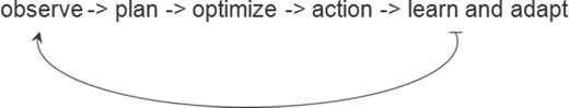
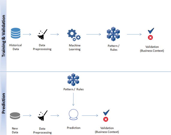
Python executes a finally clause always before leaving the try statement irrespective of an exception occurrence. If an exception clause not designed to handle the exception is raised in the try clause, the same is re-raised after the finally clause has been executed. If usage of statements such as break, continue, or return forces the program to exit the try clause, still the finally is executed on the way out. See Figure 1-3.
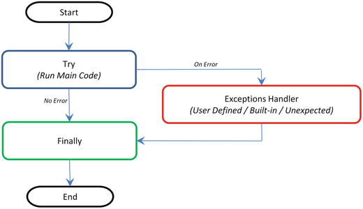
Figure 1-3. Code Flow for Error Handler
Note that generally it’s a best practice to follow a single exit point principle by using finally. This means that either after successful execution of your main code or your error handler has finished handling an error, it should pass through the finally so that the code will be exited at the same point under all circumstances.
Endnotes
With this we have reached the end of this chapter. So far I have tried to cover the basics and the essential topics to get you started in Python, and there is an abundance of online / offline resources available to increase your knowledge depth about Python as a programming language. On the same note, I would like to leave you with some useful resources for your future reference. See Table 1-17.
Table 1-17. Additional resources
Resource | Description | Mode |
|---|---|---|
This is the Python’s official tutorial, and it covers all the basics and offers a detailed tour of the language and standard libraries. | Online | |
A curated list of awesome Python frameworks, libraries, software, and resources. | Online | |
The Hacker's Guide to Python | This book is aimed at developers who already know Python but want to learn from more experienced Python developers. | Book |