Table of Contents for

Node.js in Action, Second Edition

Chapter 8. Storing application data

This chapter covers

• Relational databases: PostgreSQL
• NoSQL databases: MongoDB
• ACID categories
• Hosted cloud databases and storage services

Node.js serves an incredibly diverse set of developers with equally diverse needs. No single database or storage solution solves the number of use cases tackled by Node. This chapter provides a broad overview of the data storage possibilities, along with some important high-level concepts and terminology.

8.1. Relational databases

For most of the history of the web, relational databases have been the dominant choice for application data storage. This topic has been covered at length in many other texts and university programs, so we don’t spend too much time elaborating on this topic in this chapter.

Relational databases, built upon the mathematical ideas of relational algebra and set theory, have been around since the 1970s. A schema specifies the format of various data types and the relationships that exist among those types. For example, if you’re building a social network, you may have User and Post data types, and define a one-to-many relationship between User and Post. Then using Structured Query Language (SQL), you can issue queries on this data, such as, “Give me all posts belonging to a user with ID 123,” or in SQL: SELECT * FROM post WHERE user_id=123.

8.2. PostgreSQL

Both MySQL and PostgreSQL (Postgres) are popular relational database choices for Node applications. The differences between relational databases are mostly aesthetic, so for the most part, this section also applies to using other relational databases such as MySQL in Node. First, let’s look at how to install Postgres on your development machine.

8.2.1. Performing installation and setup

Postgres needs to be installed on your system. You can’t simply npm install it. Installation instructions vary from platform to platform. On macOS, installation is as simple as this:

brew update
brew install postgres

You may run into upgrade issues if you already have a Postgres installation. Follow the instructions for your platform to migrate your existing databases, or wipe the database directory:

# WARNING: will delete existing postgres configuration & data
rm –rf /usr/local/var/postgres

Then initialize and start Postgres:

initdb -D /usr/local/var/postgres
pg_ctl -D /usr/local/var/postgres -l logfile start

This starts a Postgres daemon. This daemon needs to be started every time you boot your computer. You may want to automatically boot the Postgres daemon on startup, and many online guides detail this process for your particular operating system.

Similarly, most Linux systems have a package for installing Postgres. With Windows, you should download the installer from postgresql.org (www.postgresql.org/download/windows/).

Several command-line administration utilities are installed with Postgres. You may want to familiarize yourself with some of them by reading their man pages.

8.2.2. Creating the database

After the Postgres daemon is running, you need to create a database to use. This needs to be done only once. The simplest way is to use createdb from the command line. Here you create a database named articles:

createdb articles

There is no output if this succeeds. If a database with this name already exists, this command does nothing and reports a failure.

Most applications connect to only a single database at a time, though multiple databases may be configured, depending on the environment the database is running in. Many applications have at least two environments: development and production.

To drop all the data from an existing database, you can run the dropdb command from a terminal, passing the database name as an argument:

dropdb articles

You need to run createdb before using this database again.

8.2.3. Connecting to Postgres from Node

The most popular package for interfacing with Postgres from node is pg. You can install pg by using npm:

npm install pg --save

With the Postgres server running, a database created, and the pg package installed, you’re ready to start using the database from Node. Before you can issue any commands against the server, you need to establish a connection to it, as shown in the next listing.

Listing 8.1. Connecting to the database

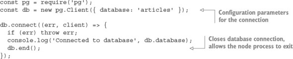
Comprehensive documentation for pg.Client and other methods can be found on the pg package’s wiki page on GitHub: https://github.com/brianc/node-postgres/wiki.

8.2.4. Defining tables

In order to store data in PostgreSQL, you first need to define some tables and the shape of the data to be stored within them, as shown in the following listing (ch08-databases/listing8_3 in the book’s source code).

Listing 8.2. Defining a schema

db.query(`
  CREATE TABLE IF NOT EXISTS snippets (
    id SERIAL,
    PRIMARY KEY(id),
    body text
  );
`, (err, result) => {
  if (err) throw err;
  console.log('Created table "snippets"');
  db.end();
});

8.2.5. Inserting data

After your table is defined, you can insert data into it by using INSERT queries, as shown in the next listing. If you don’t specify the id value, PostgreSQL will select an ID for you. To learn which ID was chosen for a particular row, you append RETURNING id to your query, and it appears in the rows of the result passed to the callback.

Listing 8.3. Inserting data

const body = 'hello world';
db.query(`
  INSERT INTO snippets (body) VALUES (
    '${body}'
  )
  RETURNING id
`, (err, result) => {
  if (err) throw err;
  const id = result.rows[0].id;
  console.log('Inserted row with id %s', id);
  db.query(`
    INSERT INTO snippets (body) VALUES (
      '${body}'
    )
    RETURNING id
  `, () => {
    if (err) throw err;
    const id = result.rows[0].id;
    console.log('Inserted row with id %s', id);
  });
});

8.2.6. Updating data

After data is inserted, you can update the data by using an UPDATE query, as shown in the next listing. The number of affected rows will be available in the rowCount property of the query result. You can find the full example for this listing in ch08-databases/listing8_4.

Listing 8.4. Updating data

const id = 1;
const body = 'greetings, world';
db.query(`
  UPDATE snippets SET (body) = (
    '${body}'
  ) WHERE id=${id};
`, (err, result) => {
  if (err) throw err;
  console.log('Updated %s rows.', result.rowCount);
});

8.2.7. Querying data

One of the most powerful features of a relational database is the ability to perform complex ad hoc queries on your data. Querying is performed by using SELECT statements, and the simplest example of this is shown in the following listing.

Listing 8.5. Querying data

db.query(`
  SELECT * FROM snippets ORDER BY id
`, (err, result) => {
  if (err) throw err;
  console.log(result.rows);
});

8.3. Knex

Many developers prefer to not work with SQL statements directly in their applications, instead using an abstraction over the top. This is understandable, given that concatenating strings into SQL statements can be a clunky process and that queries can grow hard to understand and maintain. This has been particularly true for JavaScript, which didn’t have a syntax for representing multiline strings until ES2015 introduced template literals (see https://developer.mozilla.org/en/docs/Web/JavaScript/Reference/Template_literals). Figure 8.1 shows Knex’s statistics, including the number of downloads, which demonstrates its popularity.

Figure 8.1. Knex’s usage statistics

Knex is a Node package implementing a type of lightweight abstraction over SQL, known as a query builder. A query builder constructs SQL strings though a declarative API that closely resembles the generated SQL. The Knex API is intuitive and unsurprising:

knex({ client: 'mysql' })
  .select()
  .from('users')
  .where({ id: '123' })
  .toSQL();

This produces a parameterized SQL query in the MySQL dialect of SQL:

select * from `users` where `id` = ?

8.3.1. jQuery for databases

Despite ANSI and ISO SQL standards existing since the mid-1980s, most databases still speak their own SQL dialects. PostgreSQL is a notable exception; it prides itself on adhering to the SQL:2008 standard. A query builder can normalize differences across SQL dialects, providing a single, unified interface for SQL generation for multiple technologies. This has clear benefits for teams that regularly context-switch between various database technologies.

Knex.js currently supports the following databases:

• PostgreSQL
• MSSQL
• MySQL
• MariaDB
• SQLite3
• Oracle

Table 8.1 compares the ways Knex generates an insert statement, depending on which database is selected.

Table 8.1. Comparing Knex-generated SQL for various databases

Database	SQL
PostgreSQL, SQLite, and Oracle	insert into "users" ("name", "age") values (?, ?)
MySQL and MariaDB	insert into `users` (`name`, `age`) values (?, ?)
Microsoft SQL Server	insert into [users] ([name], [age]) values (?, ?)

Knex supports promises and Node-style callbacks.

8.3.2. Connecting and running queries with Knex

Unlike many other query builders, Knex can also connect and execute queries for you against the selected database driver:

db('articles')
  .select('title')
  .where({ title: 'Today's News' })
  .then(articles => {
    console.log(articles);
  });

Knex queries return promises by default, but can also support Node’s callback convention with .asCallback:

db('articles')
  .select('title')
  .where({ title: 'Today's News' })
  .asCallback((err, articles) => {
    if (err) throw err;
    console.log(articles);
  });

In chapter 3, you interacted with a SQLite database by using the sqlite3 package directly. This API can be rewritten using Knex. To run this example, first ensure that both the knex and sqlite3 packages are installed from npm:

npm install knex@~0.12.0 sqlite3@~3.1.0 --save

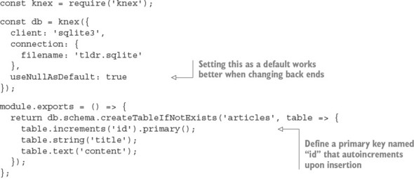
The next listing uses sqlite3 to implement a simple Article model. Save this file as db.js; you’ll use it in listing 8.7 to interact with the database.

Listing 8.6. Using Knex to connect and query sqlite3

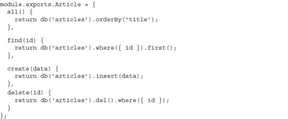
Now Article entries can be added by using db.Article. The following listing can be used with the previous one to create articles and then print them. See ch08-databases/listing8_7/index.js for the full example.

Listing 8.7. Interacting with the Knex-powered API

db().then(() => {
  db.Article.create({
    title: 'my article',
    content: 'article content'
  }).then(() => {
    db.Article.all().then(articles => {
      console.log(articles);
      process.exit();
    });
  });
})
.catch(err => { throw err });

SQLite requires minimal configuration: you don’t need to boot up a server daemon or create databases from outside the application. SQLite writes everything into a single file. If you run the preceding code, you’ll find an articles.sqlite file in your current directory. Wiping a SQLite database is as simple as deleting this one file:

rm articles.sqlite

SQLite also has an in-memory mode, which avoids writing to disk entirely. This mode is commonly used to decrease the running time of automated tests. You can configure in-memory mode by using the special :memory: filename. Opening multiple connections to the :memory: file gives each connection its own private database:

const db = knex({
  client: 'sqlite3',
  connection: {
    filename: ':memory:'
  },
  useNullAsDefault: true
});

8.3.3. Swapping the database back end

Because you’re using Knex, it’s trivial to change listings 8.6 and 8.7 to use PostgreSQL over sqlite3. Knex needs the pg package installed to talk to the PostgreSQL server, which you’ll need to have installed and running. Install the pg package into the folder with listing 8.7 (ch08-databases/listing8_7 in the book’s code) and remember to create the appropriate database by using PostgreSQL’s createdb command-line utility:

npm install pg --save
createdb articles

The only code changes required to use this new database are in the Knex configuration; otherwise, the consumer API and usage are identical:

const db = knex({
  client: 'pg',
  connection: {
    database: 'articles'
  }
})

Note that in a real-world scenario, you’d also need to migrate any existing data.

8.3.4. Beware of leaky abstractions

Query builders can normalize SQL syntax, but can do little to normalize behavior. Some features are supported in only particular databases, and some databases may exhibit entirely different behavior given identical queries. For example, the following are two methods of defining a primary key when using Knex:

• table.increments('id').primary();
• table.integer('id').primary();

Both options work as expected in SQLite3, but the second option will cause an error in PostgreSQL when inserting a new record:

"null value in column "id" violates not-null constraint"

Values inserted into SQLite with a null primary key will be assigned an automatically incremented ID, regardless of whether the primary-key column was explicitly configured to autoincrement. PostgreSQL, on the other hand, requires autoincrement columns to be defined explicitly. Many such behavioral differences exist between databases, and some differences may be subtle without visible errors. Thorough testing needs to be applied if you do choose to transition to a different database.

8.4. MySQL vs. PostgreSQL

Both MySQL and PostgreSQL are mature and powerful databases, and for many projects, there will be minimal differences when selecting one over the other. Many distinctions, which won’t be significant until the project needs to scale, exist below or at the edge of the interface exposed to the application developer.

An exhaustive comparison between relational databases is mostly beyond the scope of this book, as the topic is complicated. Some notable distinctions are listed here:

• PostgreSQL supports more-expressive data types, including arrays, JSON, and user-defined types.
• PostgreSQL has built-in full-text search.
• PostgreSQL supports the full ANSI SQL:2008 standard.
• PostgreSQL’s replication support isn’t as powerful or battle-tested as MySQL’s.
• MySQL is older and has a bigger community. More compatible tools and resources are available for MySQL.
• The MySQL community has more fragmentation through subtly different forks (for example, MariaDB and WebScaleSQL from Facebook, Google, Twitter, and so forth).
• MySQL’s pluggable storage engine can make it more complicated to understand, administer, and tune. On the other hand, this can be seen as an opportunity for more fine-grained control over performance.

MySQL and PostgreSQL express different performance characteristics at scale, depending on the type of workload. The subtleties of your workload may not become obvious until the project matures.

Many online resources provide far more in-depth comparisons between relational databases:

• www.digitalocean.com/community/tutorials/sqlite-vs-mysql-vs-postgresql-a-comparison-of-relational-database-management-systems
• https://blog.udemy.com/mysql-vs-postgresql/
• https://eng.uber.com/mysql-migration/

Which relational database you initially choose is unlikely to be a significant factor in the success of your project, so don’t worry about this decision too much. You can migrate to another database later, but Postgres should be powerful enough to provide most of the features and scalability that you’ll ever need. But if you’re in a position to evaluate several databases, you should familiarize yourself with the idea of ACID guarantees.

8.5. ACID guarantees

ACID describes a set of desirable properties for database transactions: atomicity, consistency, isolation, and durability. The exact definitions of these terms can vary. As a general rule, the more strictly a system guarantees ACID properties, the greater the performance compromise. This ACID categorization is a common way for developers to quickly communicate the trade-offs of a particular solution, such as those found in NoSQL systems.

8.5.1. Atomicity: transactions either succeed or fail in entirety

An atomic transaction can’t be partially executed: either the entire operation completes, or the database is left unchanged. For example, if a transaction is to delete all comments by a particular user, either all comments will be deleted, or none of them will be deleted. There is no way to end up with some comments deleted and some not. Atomicity should apply even in the case of system error or power failure. Atomic is used here with its original meaning of indivisible.

8.5.2. Consistency: constraints are always enforced

The completion of a successful transaction must maintain all data-integrity constraints defined in the system. Some example constraints are that primary keys must be unique, data conforms to a particular schema, or foreign keys must reference entities that exist. Transactions that would lead to inconsistent state typically result in transaction failures, though minor issues may be resolved automatically; for example, coercing data into the correct shape. This isn’t to be confused with the C of consistency in the CAP theorem, which refers to guaranteeing a single view of the data being presented to all readers of a distributed store.

8.5.3. Isolation: concurrent transactions don’t interfere

Isolated transactions should produce the same result, whether the same transactions are executed concurrently or sequentially. The level of isolation a system provides directly affects its ability to perform concurrent operations. A naïve isolation scheme is the use of a global lock, whereby the entire database is locked for the duration of a transaction, thus effectively processing all transactions in series. This gives a strong isolation guarantee but it’s also pathologically inefficient: transactions operating on entirely disjointed datasets are needlessly blocked (for example, a user adding a comment ideally doesn’t block another user updating their profile). In practice, systems provide various levels of isolation using more fine-grained and selective locking schemes (for example, by table, row, or field). More-sophisticated systems may even optimistically attempt all transactions concurrently with minimal locking, only to retry transactions by using increasingly coarse-grained locks in cases where conflicts are detected.

8.5.4. Durability: transactions are permanent

The durability of a transaction is the degree to which its effects are guaranteed to persist, even after restarts, power failures, system errors, or even hardware failures. For example, an application using the SQLite in-memory mode has no transaction durability; all data is lost when the process exits. On the other hand, SQLite persisting to disk will have good transaction durability, because data persists even after the machine is restarted.

This may seem like a no-brainer: just write the data to disk—and voila, you have durable transactions. But disk I/O is one of the slowest operations your application can perform and can quickly become a significant bottleneck in your application, even at moderate levels of scale. Some databases offer different durability trade-offs that can be employed to maintain acceptable system performance.

8.6. NoSQL

The umbrella term for data stores that don’t fit in the relational model is NoSQL. Today, because some NoSQL databases do speak SQL, the term NoSQL has a meaning closer to nonrelational or as the backronym not only SQL.

Here’s a subset of paradigms and example databases that can be considered NoSQL:

• Key-value/tuple— DynamoDB, LevelDB, Redis, etcd, Riak, Aerospike, Berkeley DB
• Graph— Neo4J, OrientDB
• Document— CouchDB, MongoDB, Elastic (formerly Elasticsearch)
• Column— Cassandra, HBase
• Time series— Graphite, InfluxDB, RRDtool
• Multiparadigm— Couchbase (document database, key/value store, distributed cache)

For a more comprehensive list of NoSQL databases, see http://nosql-database.org/.

NoSQL concepts can be difficult to digest if you’ve worked only with relational databases, because NoSQL usage often goes directly against well-established best practices: No defined schemas. Duplicate data. Loosely enforced constraints. NoSQL systems take responsibilities normally assigned to the database and place them in the realm of the application. It can all seem dirty.

Usually, only a small set of access patterns create the bulk of the workload for the database, such as the queries that generate the landing screen of your application, where multiple domain objects need to be fetched. A common technique for improving read performance in a relational database is denormalization, whereby domain queries are preprocessed and shaped into a form that reduces the number of reads required for consumption by the client.

NoSQL data is more frequently denormalized by default. The domain modeling step may be entirely skipped. This can discourage overengineering of the data model, allow changes to be executed more quickly, and lead to an overall simpler, better-performing design.

8.7. Distributed databases

An application can scale vertically by increasing the capacity of the machines running it, or horizontally by adding more machines. Vertical scaling is usually the less complicated option, but constraints borne by the hardware limit how far one machine can scale. Vertical scaling also tends to get expensive quickly. Horizontal scaling, on the other hand, has a far higher capacity for growth as you add capacity by adding more processes and more machines. This comes at the cost of complexity in orchestrating many more moving parts. All growing systems eventually reach a point where they must scale horizontally.

Distributed databases are designed from the outset with horizontal scaling as the premise. Data stored across multiple machines improves the durability of the data by removing any single point of failure. Many relational systems have some capacity to perform horizontal scaling in the form of sharding, master/slave, master/master replication, though even with these capacities, relational systems aren’t designed to scale beyond a few hundred nodes. For example, the upper limit for a MySQL cluster is 255 nodes. Distributed databases, on the other hand, can scale into the thousands of nodes by design.

8.8. MongoDB

MongoDB is a document-oriented, distributed database that’s hugely popular among Node developers. It’s the M in the fashionable MEAN stack (MongoDB, Express, Angular, Node) and is often one of the first databases people encounter when they start working with Node. Figure 8.2 shows how popular the mongodb module is on npm.

Figure 8.2. MongoDB’s usage statistics

MongoDB attracts more than its fair share of criticism and controversy; despite this, it remains a staple data store for many developers. MongoDB has known deployments in prominent companies including Adobe, LinkedIn, and eBay and is even used in a component of the Large Hadron Collider at the European Organization for Nuclear Research (CERN).

A MongoDB database stores documents in schemaless collections. Documents don’t need to have a predefined schema, and documents in a single collection needn’t share the same schema. This grants a lot of flexibility to MongoDB, though the burden is now upon the application to ensure that documents maintain a predictable structure (guaranteeing consistency—the C in ACID).

8.8.1. Performing installation and setup

MongoDB needs to be installed on your system. Installation varies between platforms. On macOS, installation is as simple as this:

brew install mongodb

The MongoDB server is started by using the mongod executable:

mongod --config /usr/local/etc/mongod.conf

The most popular MongoDB driver is the official mongodb package by Christian Amor Kvalheim:

npm install mongodb@^2.1.0 --save

Windows users should note that driver installation requires msbuild.exe, which is installed by Microsoft Visual Studio.

8.8.2. Connecting to MongoDB

After installing the mongodb package and starting the mongod server, you can connect as a client from Node, as shown in the following listing.

Listing 8.8. Connecting to MongoDB

const { MongoClient } = require('mongodb');

MongoClient.connect('mongodb://localhost:27017/articles')
  .then(db  => {
    console.log('Client ready');
    db.close();
  }, console.error);

The connection’s success handler is passed a database client instance, from which all database commands are executed.

Most interactions with the database are via the collection API:

• collection.insert(doc)—Insert one or more documents
• collection.find(query)—Find documents matching the query
• collection.remove(query)—Remove documents matching the query
• collection.drop()—Remove the entire collection
• collection.update(query)—Update documents matching the query
• collection.count(query)—Count documents matching the query

Operations such as find, insert, and delete come in a few flavors, depending on whether you’re operating on one or many values. For example:

• collection.insertOne(doc)—Insert a single document
• collection.insertMany([doc1, doc2])—Insert many documents
• collection.findOne(query)—Find a single document matching the query
• collection.updateMany(query)—Update all documents matching the query

8.8.3. Inserting documents

collection.insertOne places a single object into the collection as a document, as shown in the next listing. The success handler is passed an object containing metadata about the state of the operation.

Listing 8.9. Inserting a document

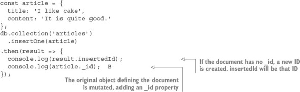
The insertMany call is similar, except it takes an array of multiple documents. The insertMany response will contain an array of insertedIds, in the order the documents were supplied, instead of a singular insertedId.

8.8.4. Querying

Methods that read documents from the collection (such as find, update, and remove) take a query argument that’s used to match documents. The simplest form of a query is an object with which MongoDB will match documents with the same structure and same values. For example, this finds all articles with the title “I like cake”:

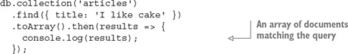
Queries can be used to match objects by their unique _id:

collection.findOne({ _id: someID })

Or match based on a query operator:

Many query operators exist in the MongoDB query language—for example:

• $eq—Equal to a particular value
• $neq—Not equal to a particular value
• $in—In array
• $nin—Not in array
• $lt, $lte, $gt, $gte—Greater/less than or equal to comparison
• $near—Geospatial value is near a certain coordinate
• $not, $and, $or, $nor—Logical operators

These can be combined to match almost any condition and create a highly readable, sophisticated, and expressive query language. See https://docs.mongodb.com/-manual/reference/operator/query/ for more information on queries and query operators.

The next listing shows an example that the previous Articles API implemented by using MongoDB, while maintaining a nearly identical external interface. Save this file as db.js (it’s listing8_10/db.js in the book’s sample code).

Listing 8.10. Implementing the Article API with MongoDB

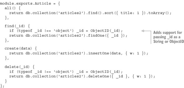
The following snippet shows how to use listing 8.10 (listing 8_10/index.js in the sample code):

const db = require('./db');

db().then(() => {
  db.Article.create({ title: 'An article!' }).then(() => {
    db.Article.all().then(articles => {
      console.log(articles);
      process.exit();
    });
  });
});

This uses a promise from listing 8.10 to connect to the database, then creates an article using Article’s create method. After that, it loads all articles and logs them out.

8.8.5. Using MongoDB identifiers

Identifiers from MongoDB are encoded in Binary JSON (BSON) format. The _id property on a document is a JavaScript Object that wraps a BSON-formatted ObjectID value. MongoDB uses BSON to represent documents internally and as a transmission format. BSON is more space-efficient than JSON and can be parsed more quickly, which means faster database interactions using less bandwidth.

A BSON ObjectID isn’t just a random sequence of bytes; it encodes metadata about where and when the ID was generated. For example, the first four bytes of an ObjectID are a timestamp. This removes the need to have to store a createdAt timestamp property in your documents:

See https://docs.mongodb.com/manual/reference/method/ObjectId/ for more information about the ObjectID format.

ObjectIDs may superficially appear to be strings because of the way they’re printed in the terminal, but they’re objects. ObjectIDs suffer from classic object comparison gotchas: seemingly totally equivalent values are reported as inequivalent because they reference different objects.

In the following snippet, we extract the same value twice. Using the node’s built-in assert module, we try to assert that the objects or the IDs are equivalent, but both result in failure:

const Articles = db.collection('articles');
Articles.find().then(articles => {
  const article1 = articles[0];
  return Articles
    .findOne({_id: article1._id})
    .then(article2 => {
      assert.equal(article2._id, article1._id);
    });
});

These assertions produce error messages that at first seem confusing, as the actual values appear to match the expected values:

operator: equal
expected: 577f6b45549a3b991e1c3c18
actual:   577f6b45549a3b991e1c3c18
operator: equal
expected:
  { _id: 577f6b45549a3b991e1c3c18, title: 'attractive-money' ... }
actual:
  { _id: 577f6b45549a3b991e1c3c18, title: 'attractive-money' ... }

Equivalence can be detected correctly by using the ObjectID’s equal method that’s available on every _id. Alternatively, you can coerce the identifiers and compare them as strings, or use a deepEquals method such as that found on Node’s built-in assert module:

Identifiers passed to the Node mongodb driver must be a BSON-formatted ObjectID. A string can be converted into an ObjectID by using the ObjectID constructor:

const { ObjectID } = require('mongodb');
const stringID = '577f6b45549a3b991e1c3c18';
const bsonID = new ObjectID(stringID);

Where possible, the BSON form should be maintained; the cost of marshalling to and from strings works against the potential performance gains MongoDB hopes to achieve by serving client identifiers as BSON. See http://bsonspec.org/ for detailed information about the BSON format.

8.8.6. Using replica sets

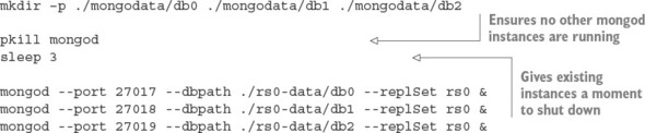
The distributed features of MongoDB are mostly beyond the scope of this book, but in this section we quickly cover the basics of replica sets. Many mongod processes can be run as nodes/members of a replica set. A replica set consists of a single primary node and numerous secondary nodes. Each member of a replica set needs to be allocated a unique port and directory to store its data. Instances can’t share ports or directories, and the directories must already exist before startup.

In the following listing, you create a unique directory for each member and start them on a sequential port number starting from 27017. You may want to run each of the mongod commands in a new terminal tab without backgrounding them (without the trailing &).

Listing 8.11. Starting a replica set

After the replica set is running, MongoDB needs to perform some initiation. You need to connect to the port of the instance that you want to become the first primary node (27017 by default) and call rs.initiate(), as shown in the following listing. Then you need to add each instance as a member of the replica set. Note that you need to supply the hostname of the machine you’re connecting to.

Listing 8.12. Initiating a replica set

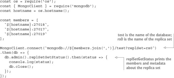
MongoDB clients need to know about all the possible replica set members when they connect, though not all members need to currently be online. After connecting, you may use the MongoDB client as usual. Listing 8.13 shows how to create a replica set with three members.

Listing 8.13. Connecting to a replica set

If any of the mongod nodes crash, the system will continue working, as long as at least two instances are running. If the primary node crashes, a secondary node will automatically be elected to be promoted into the primary.

8.8.7. Understanding write concerns

MongoDB gives the developer fine-grained control over which performance and safety trade-offs are acceptable for various areas of your application. It’s important to understand the concepts of both write and read concerns in order to use MongoDB without surprises, especially as the number of nodes in your replica set increases. In this section, we touch only on write concerns, as they’re the most important.

Write concerns dictate the number of mongod instances that the data needs to be successfully written to before the overall operation responds with a success. If not explicitly specified, the default write concern is 1, which ensures that the data has been written to at least one node. It may not provide an adequate level of assurance for critical data; data may be lost if the node goes down before replicating to other nodes.

It’s possible and often desirable to set a zero write concern, whereby the application doesn’t wait for any response:

db.collection('data').insertOne(data, { w: 0 });

A zero write concern grants the highest performance but provides the least durability assurances, and is typically used for only temporary or unimportant data (such as the writing of logs or caches).

If you’re connected to a replica set, you can indicate a write concern greater than 1. Replicating to more nodes decreases the likelihood of data loss, at the expense of more latency when performing operations:

db.collection('data').insertOne(data, { w: 2 });
db.collection('data').insertOne(data, { w: 5 });

You may want to scale the write concern as the number of nodes in the cluster changes. This can be done dynamically by MongoDB itself if you set the write concern to majority. This ensures that data is written to more than 50% of the available nodes:

db.collection('data').insertOne(data, { w: 'majority' });

The default write concern of 1 may not provide an adequate level of assurance for critical data. Data may be lost if the node goes down before replicating to other nodes.

Setting a write concern higher than 1 ensures that the data exists across multiple mongod instances before continuing. Running multiple instances on the same machine adds protection but doesn’t help in the case of systemwide failures such as running out of disk space or RAM. You can protect against machine failure by running instances across multiple machines and ensuring that writes propagate to these nodes, but this again will be slower and doesn’t protect against datacenter-wide failure. Running nodes across different datacenters protects against datacenter outage, but ensuring that data is replicated across datacenters will greatly impact performance.

As always, the more assurances you add, the slower and more complicated the system becomes. This isn’t an issue specific to MongoDB; it’s an issue with any and all data storage. No perfect solution exists, and you’ll need to decide the acceptable level of risk for the various parts of your application.

For more information about how MongoDB replication works, see the following resources:

• https://docs.mongodb.com/manual/faq/replica-sets/
• https://docs.mongodb.com/manual/faq/concurrency/

8.9. Key/value stores

Each record in a key/value store comprises a single key and a single value. In many key/value systems, values can be of any data type, of any length or structure. From the perspective of the database, values are opaque atoms: the database doesn’t know or care about the type of the data and can’t be subdivided or accessed other than in its entirety. Contrast this with value storage in a relational database: data is stored in a series of tables, which contain rows of data separated into predefined columns. In a key/value store, the responsibility of managing the format of the data is handed to the application.

Key/value stores can often be found in performance-critical paths of an application. Ideally, values are laid out in a manner such that the absolute minimum number of reads is required to fulfill a task. Key/value stores come with simpler querying capabilities than other database types. Ideally, complex queries are precalculated; otherwise, they need to be performed within the application rather than the database. This constraint can lead to easily understood and predictable performance characteristics.

The most popular key/value stores, such as Redis and Memcached, are often used for volatile storage (if the process exits, the data is lost). Avoiding writing to disk is one of the best ways to improve performance. This can be an acceptable trade-off for features when data can be regenerated or loss is of little concern; for example, caches and user sessions.

Key/value stores may carry a stigma that they can’t be used for primary storage, but this isn’t always true. Many key/value stores provide just as much durability as a “real” database.

8.10. Redis

Redis is a popular in-memory, data-structure store. Although many consider Redis to be a key/value store, keys and values represent only a subset of the features Redis supports across a variety of useful, basic data structures. Figure 8.3 shows the usage statistics for the redis package on npm.

Figure 8.3. The redis package’s statistics on npm

The data structures built into Redis include the following:

• Strings
• Hashes
• List
• Set
• Sorted set

Redis also comes with many other useful features out of the box:

• Bitmap data— Direct bit manipulation in values.
• Geospatial indexes— Storing geospatial data with radius queries.
• Channels— A publish/subscribe data-delivery mechanism.
• TTLs— Values can be configured with an expiry time, after which they’re automatically removed.
• LRU eviction— Optionally removes values that haven’t been recently used in order to maintain maximum memory usage.
• HyperLogLog— High-performing approximation of set cardinality, while maintaining a low-memory footprint (doesn’t need to store every member).
• Replication, clustering, and partitioning— Horizontal scaling and data durability.
• Lua scripting— Extend Redis with custom commands.

In this section, you’ll find several bulleted lists of Redis commands. They’re not intended to be a reference, but rather to give some insight into what’s possible with Redis. It’s an incredibly powerful and versatile tool. See http://redis.io/commands for more details.

8.10.1. Performing installation and setup

Redis can be installed through your system’s package management tool. On macOS, you can easily install it with Homebrew:

brew install redis

Starting the server is done using the redis-server executable:

redis-server /usr/local/etc/redis.conf

The server listens on port 6379 by default.

8.10.2. Performing initialization

A Redis client instance is created with the createClient function from the redis npm package:

const redis = require('redis');
const db = redis.createClient(6379, '127.0.0.1');

This function takes the port and a host as arguments. But if you’re running the Redis server on the default port on your local machine, you don’t need to supply any arguments at all:

const db = redis.createClient();

The Redis client instance is an EventEmitter, so you can attach listeners for various Redis status events, as shown in the next listing. You can immediately start issuing commands to the client, and they’ll be buffered until the connection is ready.

Listing 8.14. Connecting to Redis and listening for status events

const redis = require('redis');

const db = redis.createClient();
db.on('connect', () => console.log('Redis client connected to server.'));
db.on('ready', () => console.log('Redis server is ready.'));
db.on('error', err => console.error('Redis error', err));

The error handler will fire if a connection or client problem occurs. If an error event is fired and no error handler is attached, the application process will throw the error and crash; this is a feature of all EventEmitters in Node. If the connection fails and an error handler is supplied, the Redis client will attempt to retry the connection.

8.10.3. Working with key/value pairs

Redis can be used as a generic key/value store for strings and arbitrary binary data. Reading and writing a key/value pair can be done using the set and get methods, respectively:

db.set('color', 'red', err => {
  if (err) throw err;
});

db.get('color', (err, value) => {
  if (err) throw err;
  console.log('Got:', value);
});

If you set an existing key, the value will be overwritten. If you try to get a key that doesn’t exist, the value will be null; it’s not considered an error.

The following commands can be used to retrieve and manipulate values:

• append
• decr
• decrby
• get
• getrange
• getset
• incr
• incrby
• incrbyfloat
• mget
• mset
• msetnx
• psetex
• set
• setex
• setnx
• setrange
• strlen

8.10.4. Working with keys

You can check whether a key exists by using exists. This works with any data type:

db.exists('users', (err, doesExist) => {
  if (err) throw err;   console.log('users exists:', doesExist);
});

Along with exists, the following commands can all be used with any key, regardless of the type of the value (these commands work with strings, sets, lists, and so forth):

• del
• exists
• rename
• renamenx
• sort
• scan
• type

8.10.5. Encoding and data types

The Redis server stores keys and values as binary objects; it’s not dependent on the encoding of the value passed to the client. Any valid JavaScript string (UCS2/UTF16) can be used as a valid key or value:

db.set('greeting', '你好', redis.print);
db.get('greeting', redis.print);
db.set('icon', '?', redis.print);
db.get('icon', redis.print);

By default, keys and values are coerced to strings as they’re written. For example, if you set a key with a number, it will be a string when you try to get that same key:

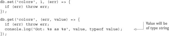
The Redis client silently coerces numbers, Booleans, and dates into strings, and it also happily accepts buffer objects. Trying to set any other JavaScript type as a value (for example, Object, Array, RegExp) prints a warning that should be heeded:

db.set('users', {}, redis.print);

Deprecated: The SET command contains a argument of type Object.
This is converted to "[object Object]" by using .toString() now
  and will return an error from v.3.0 on.
Please handle this in your code to make sure everything works
  as you intended it to.

In the future, this will be an error, so the calling application must be responsible for ensuring that the correct types are passed to the Redis client.

Gotcha: single vs. multiple value arrays

The client produces a cryptic error, “ReplyError: ERR syntax error,” if you try to set an array of values:

db.set('users', ['Alice', 'Bob'], redis.print);

But note that no error occurs when the array contains only a single value:

db.set('user', ['Alice'], redis.print);
db.get('user', redis.print);

This type of bug may show symptoms only when you’re running it in production, as it can easily elude detection if the test suite happens to produce only single-valued arrays, which is common for stripped-down test data. Be aware!

Binary data with buffers

Redis is capable of storing arbitrary byte data, which means you can store any type of data in it. The Node client supports this feature with special handling for Node’s Buffer type. When a buffer is passed to the Redis client as a key or value, the bytes are sent unmodified to the Redis server. This avoids accidental data corruption and performance penalties of unnecessary marshalling between strings and buffers. For example, if you want to write data from disk or network directly into Redis, it’s more efficient to write the buffers directly to Redis than to convert them into strings first.

Redis has recently added commands for manipulating individual bits of string values, which can be of use when working with buffers:

• bitcount
• bitfield
• bitop
• setbit
• bitpos

8.10.6. Using hashes

A hash is a collection of key/value pairs. The hmset command takes a key and an object representing the key/value pairs of the hash. You can get the key/value pairs back as an object by using hmget, as shown in the next listing.

Listing 8.15. Storing data in elements of Redis hashes

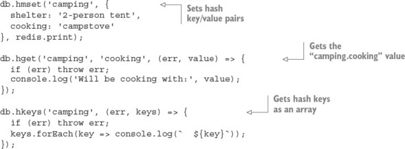
You can’t store nested objects in a Redis hash. It provides only a single level of keys and values.

The following commands operate on hashes:

• hdel
• hexists
• hget
• hgetall
• hincrby
• hincrbyfloat
• hkeys
• hlen
• hmget
• hmset
• hset
• hsetnx
• hstrlen
• hvals
• hscan

8.10.7. Using lists

A list is an ordered collection of string values. A list can contain multiple copies of the same value. Lists are conceptually similar to arrays. Lists are best used for their ability to behave as a stack (LIFO: last in, first out) or queue (FIFO: first in, first out) data structures.

The following code shows the storage and retrieval of values in a list. The lpush command adds a value to a list. The lrange command retrieves a range of values, using start and end indices. The -1 argument in the following code signifies the last item of the list, so this use of lrange retrieves all list items:

client.lpush('tasks', 'Paint the bikeshed red.', redis.print);
client.lpush('tasks', 'Paint the bikeshed green.', redis.print);
client.lrange('tasks', 0, -1, (err, items) => {
  if (err) throw err;
  items.forEach(item => console.log(`  ${item}`));
});

Lists don’t contain any built-in means to determine whether a value is in the list, or any means of discovering the index of a particular value in the list. You can manually iterate over the list to obtain this information, but this is a highly inefficient approach that should be avoided. If you need these types of features, you should consider a different data structure, such as a set, perhaps even used in addition to a list. Duplicating data across multiple data structures is often desirable in order to take advantage of various performance characteristics.

The following commands operate on lists:

• blpop
• brpop
• lindex
• linsert
• llen
• lpop
• lpush
• lpushx
• lrange
• lrem
• lset
• ltrim
• rpop
• rpush
• rpushx

8.10.8. Using sets

A set is an unordered collection of unique values. Testing membership, and adding and removing items from a set can be performed in O(1) time, making it a high-performing structure suitable for many tasks:

db.sadd('admins', 'Alice', redis.print);
db.sadd('admins', 'Bob', redis.print);
db.sadd('admins', 'Alice', redis.print);
db.smembers('admins', (err, members) => {
  if (err) throw err;
  console.log(members);
});

The following commands operate on Redis sets:

• sadd
• scard
• sdiff
• sdiffstore
• sinter
• sinterstore
• sismember
• smembers
• spop
• srandmember
• srem
• sunion
• sunionstore
• sscan

8.10.9. Providing pub/sub with channels

Redis goes beyond the traditional role of a data store by providing channels. Channels are a data-delivery mechanism that provides publish/subscribe functionality, as shown conceptually in figure 8.4. They can be useful for real-time applications such as chat and gaming.

Figure 8.4. Redis channels provide an easy solution to a common data-delivery scenario.

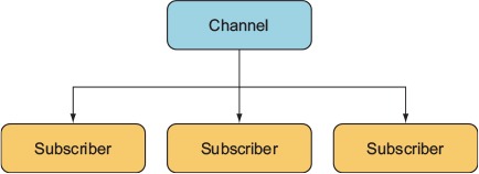
A Redis client can subscribe or publish to a channel. A message published to a channel will be delivered to all subscribers. A publisher doesn’t need to know about the subscribers, nor the subscribers about the publishers. This decoupling of publishers and subscribers is what makes this a powerful and clean pattern.

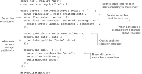
The following listing shows an example of how Redis’s publish/subscribe functionality can be used to implement a TCP/IP chat server.

Listing 8.16. A simple chat server implemented with Redis pub/sub functionality

8.10.10. Improving Redis performance

The hiredis npm package is a native binding from JavaScript to the protocol parser in the official Hiredis C library. Hiredis can significantly improve the performance of Node Redis applications, particularly if you’re using sunion, sinter, lrange, and zrange operations with large datasets.

To use hiredis, simply install it alongside the redis package in your application, and the Node redis package will detect it and use it automatically the next time it starts:

npm install hiredis --save

There are few downsides to using hiredis, but because it’s compiled from C code, some complications or limitations may arise when building hiredis for some platforms. As with all native add-ons, you may need to rebuild hiredis with npm rebuild after updating Node.

8.11. Embedded databases

An embedded database doesn’t require the installation or administration of an external server. It runs embedded within your application process itself. Communication with an embedded database usually occurs via direct procedure calls in your application, rather than across an interprocess communication (IPC) channel or a network.

In many situations, an application needs to be self-contained, so an embeddable database is the only option (for example, mobile or desktop applications). Embedded databases can also be used on web servers, often found powering high-throughput features such as user sessions or caching, and sometimes even as the primary storage.

Some embeddable databases commonly used in Node and Electron apps are as follows:

• SQLite
• LevelDB
• RocksDB
• Aerospike
• EJDB
• NeDB
• LokiJS
• Lowdb

NeDB, LokiJS, and Lowdb are all written in pure JavaScript, which by nature makes them embeddable into Node/Electron applications. Most embedded databases are simple key/value or document stores, though SQLite is a notable exception as an embeddable relational store.

8.12. LevelDB

LevelDB is an embeddable, persistent key/value store developed in early 2011 by Google, initially for use as the backing store for the IndexedDB implementation in Chrome. LevelDB’s design is built on concepts from Google’s Bigtable database. LevelDB is comparable to databases such as Berkley DB, Tokyo/Kyoto Cabinet, and Aerospike, but in the context of this book, you can think of LevelDB as an embeddable Redis with only the bare minimum of features. Like many embedded databases, LevelDB isn’t multithreaded and doesn’t support multiple instances using the same underlying file storage, so it doesn’t work in a distributed setting without a wrapping application.

LevelDB stores arbitrary byte arrays, sorted lexicographically by key. Values are compressed by using Google’s Snappy compression algorithm. Data is always persisted to disk; the total data capacity isn’t constrained by the amount of RAM on the machine, unlike an in-memory store such as Redis.

Only a small set of self-explanatory operations are provided with LevelDB: Get, Put, Del, and Batch. LevelDB can also capture snapshots of the current database state and create bidirectional iterators for moving forward or backward through the dataset. Creating an iterator creates an implicit snapshot; the data an iterator can see can’t be changed by subsequent writes.

LevelDB forms the foundation for other databases, in the form of LevelDB forks. The number of significant LevelDB offshoots could be attributed to the simplicity of LevelDB itself:

• RocksDB by Facebook
• HyperLevelDB by Hyperdex
• Riak by Basho
• leveldb-mcpe by Mojang (creators of Minecraft)
• bitcoin/leveldb for the bitcoind project

For more information about LevelDB, see http://leveldb.org/.

8.12.1. LevelUP and LevelDOWN

LevelDB support in Node is provided by the LevelUP and LevelDOWN packages written by Node foundation chair and prolific Australian developer Rod Vagg. LevelDOWN is a simple, sugar-free C++ binding to LevelDB for Node, and it’s unlikely you’ll interface with it directly. LevelUP wraps the LevelDOWN API with a more convenient, idiomatic node interface, adding support for key/value encodings, JSON, buffering writes until the database is open, and wrapping the LevelDB iterator interface in a Node stream. Figure 8.5 shows levelup’s popularity on npm.

Figure 8.5. The levelup package’s statistics on npm

8.12.2. Installation

A major convenience of using LevelDB in your Node application is that it’s embedded: you can install everything you need solely with npm. You don’t need to install any additional software; just issue the following command and you’re ready to start using LevelDB:

npm install level --save

The level package is a simple convenience wrapper around the LevelUP and LevelDOWN packages, providing a LevelUP API preconfigured to use a LevelDown back end. Documentation for the LevelUP API exposed by the level package can be found on the LevelUP readme:

• www.npmjs.com/package/levelup
• www.npmjs.com/package/leveldown

8.12.3. API overview

The LevelDB client’s main methods for storing and retrieving values are as follows:

• db.put(key, value, callback—Store a value under key
• db.get(key, callback)—Get the value under key
• db.del(key, callback)—Remove the value under key
• db.batch().write()—Perform batch operations
• db.createKeyStream(options)—Stream of keys in database
• db.createValueStream(options)—Stream of values in database

8.12.4. Initialization

When you initialize level, you need to provide a path to the directory that will store the data, as shown in the following listing; the directory will be created if it doesn’t already exist. There’s a loose community convention of giving this directory a .db extension (for example, ./app.db).

Listing 8.17. Initializing a level database

const level = require('level');

const db = level('./app.db', {
  valueEncoding: 'json'
});

After level() is called, the returned LevelUP instance is immediately ready to start accepting commands, synchronously. Commands issued before the LevelDB store is open will be buffered until the store is open.

8.12.5. Key/value encodings

Because LevelDB can store arbitrary data of any type for both keys and values, it’s up to the calling application to handle data serialization and deserialization. LevelUp can be configured to encode keys and values by using the following data types out of the box:

• utf8
• json
• binary
• id
• hex
• ascii
• base64
• ucs2
• utf16le

By default, both keys and values are encoded as UTF-8 strings. In listing 8.17, keys will remain as UTF-8 strings, but values are encoded/decoded as JSON. JSON encoding permits storage and retrieval of structured values such as objects or arrays in a somewhat similar fashion to that of a document store such as MongoDB. But note that unlike a real document store, there’s no way to access keys within values with vanilla LevelDB; values are opaque. Users can also supply their own custom encodings—for example, to support a different structured data format such as MessagePack.

8.12.6. Reading and writing key/value pairs

The core API is simple: use put(key, value) to write a value, get(key) to read a value, and del(key) to delete a value, as shown in the next listing. The code in listing 8.18 should be appended to the code in listing 8.17; for a full example, see ch08-databases/listing8_18/index.js in the book’s sample code.

Listing 8.18. Reading and writing values

const key = 'user';
const value = {
  name: 'Alice'
};

db.put(key, value, err => {
  if (err) throw err;
  db.get(key, (err, result) => {
    if (err) throw err;
    console.log('got value:', result);
    db.del(key, (err) => {
      if (err) throw err;
      console.log('value was deleted');
    });
  });
});

If you put a value on a key that already exists, the old value will be overwritten. Trying to get a key that doesn’t exist will result in an error. This error object will be of a particular type, NotFoundError, and has a special property, err.notFound, that can be used to differentiate it from other types of errors. This may seem unusual, but because LevelDB doesn’t have a built-in method to check for existence, LevelUp needs to be able to disambiguate nonexistent values and values that are undefined. Unlike with get, trying to del a nonexistent key will not cause an error.

Listing 8.19. Getting keys that don’t exist

db.get('this-key-does-not-exist', (err, value) => {
  if (err && !err.notFound) throw err;
  if (err && err.notFound) return console.log('Value was not found.');
  console.log('Value was found:', value);
});

All data reading and writing operations take an optional options argument for overriding the encoding options of the current operation, as shown in the next listing.

Listing 8.20. Overriding encoding for specific operations

const options = {
  keyEncoding: 'binary',
  valueEncoding: 'hex'
};

db.put(new Uint8Array([1, 2, 3]), '0xFF0099', options, (err) => {
  if (err) throw err;
  db.get(new Uint8Array([1, 2, 3]), options, (err, value) => {
    if (err) throw err;
    console.log(value);
  });
});

8.12.7. Pluggable back ends

A happy side effect of the separation of LevelUP/LevelDOWN is that LevelUP isn’t restricted to using LevelDB as the storage back end. Anything you can wrap with the MemDown API can be used as a storage back end for LevelUP, allowing you to use the exact same API to interface with many data stores.

Some examples of alternative back ends are as follows:

• MySQL
• Redis
• MongoDB
• JSON files
• Google spreadsheets
• AWS DynamoDB
• Windows Azure table storage
• Browser web storage (IndexedDB/localStorage)

This ability to easily swap out the storage medium or even write your own custom back end means you can use a single, consistent set of database APIs and tooling across many situations and environments. One database API to rule them all!

A commonly used alternative back end is memdown, which stores values entirely in memory rather than disk, akin to using SQLite in-memory mode. This can be particularly useful in a test environment to reduce the cost of test setup and teardown.

To run the following listing, make sure you have the LevelUP and memdown packages installed:

npm install --save levelup memdown

Listing 8.21. Using memdown with LevelUP

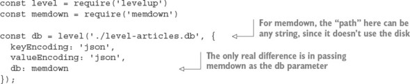
In this sample, you could’ve used the same level package you used before, because it’s just a wrapper for LevelUP. But if you’re not using the LevelDB-backed LevelDOWN that comes bundled with level, you can just use LevelUP and avoid the binary dependency on LevelDB via LevelDOWN.

8.12.8. The modular database

LevelDB’s performance and minimalism resonate with many Node developers, and it has fostered a modular database movement within the Node community. The concept is to be able to pick and choose exactly which features your application needs and tailor a database for your specific use case.

Here are just a few examples of modular LevelDB functionality available through npm packages:

• Atomic updates
• Autoincrementing keys
• Geospatial queries
• Live update streams
• LRU eviction
• Map/reduce jobs
• Master/master replication
• Master/slave replication
• SQL queries
• Secondary indexes
• Triggers
• Versioned data

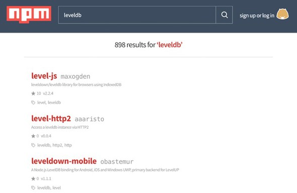
The LevelUP wiki maintains a fairly comprehensive overview of the LevelDB ecosystem: https://github.com/Level/levelup/wiki/Modules, or you can search for leveldb on npm, for which there are 898 packages at the time of this writing. Figure 8.6 shows how popular LevelDB is on npm.

Figure 8.6. Examples of third-party LevelDB packages on npm

8.13. Serialization and deserialization are expensive

It’s important to remember that the built-in JSON operations are both expensive and blocking; your process can’t do anything else while it’s marshalling data to and from JSON. The same goes for most other serialization formats. It’s common for serialization to be a key bottleneck on a web server. The best way to reduce its impact is to minimize how often it’s performed and how much data it needs to handle.

You may experience some speed improvement by using a different serialization format (for example, MessagePack or Protocol Buffers), but alternative formats should be considered only after you've squeezed the possible gains out of reducing the payload sizes and unnecessary serialization/deserialization steps.

JSON.stringify and JSON.parse are native functions and have been thoroughly optimized, but they can easily be overwhelmed when needing to handle megabytes of data. To demonstrate, the following listing benchmarks serializing and deserializing about 10 MB of data.

Listing 8.22. Serialization benchmarking

const bytes = require('pretty-bytes');
const obj = {};
for (let i = 0; i < 200000; i++) {
  obj[i] = {
    [Math.random()]: Math.random()
  };
}

console.time('serialise');
const jsonString = JSON.stringify(obj);
console.timeEnd('serialise');
console.log('Serialised Size', bytes(Buffer.byteLength(jsonString)));
console.time('deserialise');
const obj2 = JSON.parse(jsonString);
console.timeEnd('deserialise');

On a 2015 3.1 GHz Intel Core i7 MacBook Pro running Node 6.2.2, it takes roughly 140 ms to serialize, and 335 ms to deserialize, the approximately 10 MB of data. This would be a disaster if such a load were to occur on a web server, because these steps are totally blocking and have to be processed in series. Such a server would be able to handle only about a dismal seven requests a second when serializing, and about three requests a second when deserializing.

8.14. In-browser storage

The asynchronous programming model used in Node works well for many use cases because the assumption holds that I/O is the single biggest bottleneck for most web applications. The single most significant thing you can do to simultaneously reduce server workload and improve user experience is to take advantage of client-side data storage. A happy user is one who doesn’t have to wait for a full network round-trip to get results. Client-side storage can also facilitate improved application availability by allowing your application to remain at least semifunctional while the user or your service is offline.

8.14.1. Web storage: localStorage and sessionStorage

Web storage defines a simple key/value store and has great support across both desktop and mobile browsers. Using web storage, a domain can persist a moderate amount of data in the browser and retrieve it at a later time, even after the website has been refreshed, the tab closed, or the browser shut down. Web storage is your first resort for client-side persistence. Its winning feature is its bare simplicity.

There are two web storage APIs: localStorage and sessionStorage. sessionStorage implements an identical API to localStorage, though it differs in its persistence behavior. Like localStorage, data stored in sessionStorage is persisted across page reloads, but unlike localStorage, all sessionStorage data expires when the page session ends (when the tab or browser is closed). sessionStorage data can’t be accessed from different browser windows.

The web storage APIs were developed to overcome limitations with browser cookies. Specifically, cookies aren’t well suited for sharing data between multiple active tabs on the same domain. If a user is performing an activity across multiple tabs, sessionStorage can be used for sharing state between those tabs, without requiring the use of the network.

Cookies are also ill-suited for handling more long-term data that should live across multiple sessions, tabs, and windows; for example, user-authored documents or email. This is the use case that localStorage was designed to handle. Depending on the particular browser, varying upper limits exist for the amount of data that can be stored in web storage. Mobile browsers are limited to just 5 MB of storage.

API overview

The localStorage API provides the following methods for working with keys and values:

• localStorage.setItem(key, value)—Store a value under key
• localStorage.getItem(key)—Get the value under key
• localStorage.removeItem(key)—Remove the value under key
• localStorage.clear()—Remove all keys and values
• localStorage.key(index)—Get value at index
• localStorage.length—Total number of keys in localStorage

8.14.2. Reading and writing values

Both keys and values must be strings. If you pass a value that isn’t a string, it’ll be coerced into a string for you. This conversion doesn’t produce JSON strings; instead, it’s a naïve conversion using .toString. Objects will end up serialized as the string [object Object]. The application must serialize values to and from strings in order to store more-complicated data types in web storage. The next listing shows how to store JSON in localStorage.

Listing 8.23. Storing JSON in web storage

const examplePreferences = {
  temperature: 'Celcius'
};

// serialize on write
localStorage.setItem('preferences', JSON.stringify(examplePreferences));

// deserialize on read
const preferences = JSON.parse(localStorage.getItem('preferences'));
console.log('Loaded preferences:', preferences);

Access to web storage data is reasonably fast, though it’s also synchronous. Web storage blocks the UI thread while performing read and write operations. For small workloads, this overhead will be unnoticeable, but care should be taken to avoid excessive reads or writes, especially with large quantities of data. Unfortunately, web storage is also unavailable from web workers, so all reads and writes must happen on the main UI thread. For a detailed analysis of the performance impact of various client-side storage technologies, see this post by Nolan Lawson, author of PouchDB: http://nolanlawson.com/2015/09/29/indexeddb-websql-localstorage-what-blocks-the-dom/.

Web storage APIs provide no built-in facilities to perform queries, select keys by range, or search through values. You’re limited to accessing items key by key. To perform searches, you can set up and maintain your own indexes; or if your dataset is small enough, you can iterate over it in its entirety. The following listing iterates over all the keys in localStorage.

Listing 8.24. Iterating over entire dataset in localStorage

function getAllKeys() {
  return Object.keys(localStorage);
}

function getAllKeysAndValues() {
  return getAllKeys()
    .reduce((obj, str) => {
      obj[str] = localStorage.getItem(str);
      return obj;
    }, {});
}

// Get all values
const allValues = getAllKeys().map(key => localStorage.getItem(key));

// As an object
console.log(getAllKeysAndValues());

As in most key/value stores, there’s only a single namespace for keys. For example, if you have posts and comments, there’s no way to create separate stores for posts and comments. It’s easy enough to create your own “namespace” by using a prefix on each key to delineate namespaces, as shown in the next listing.

Listing 8.25. Namespacing keys

localStorage.setItem(`/posts/${post.id}`, post);
localStorage.setItem(`/comments/${comment.id}`, comment);

To get all items within a namespace, you can filter through all items using the preceding getAllKeys function, as shown in the next listing.

Listing 8.26. Getting all items in a namespace

function getNamespaceItems(namespace) {
  return getAllKeys().filter(key => key.startsWith(namespace));
}
console.log(getNamespaceItems('/exampleNamespace'));

Note that this loops over every single key in localStorage, so be wary of performance when iterating over many items.

As a result of the localStorage API being synchronous, a few restrictions exist on when and where it can be used. For example, you could use localStorage to permanently memoize the result of any function that takes and returns JSON-serializable data, as shown in the following listing.

Listing 8.27. Using localStorage for persistent memoization

// subsequent calls with the same argument will fetch the memoized result
function memoizedExpensiveOperation(data) {
  const key = `/memoized/${JSON.stringify(data)}`;
  const memoizedResult = localStorage.getItem(key);
  if (memoizedResult != null) return memoizedResult;
  // do expensive work
  const result = expensiveWork(data);
  // save result to localStorage, never calculate again
  localStorage.setItem(key, result);
  return result;
}

Note that an operation would need to be particularly slow in order for the memoization benefits to outweigh the overhead of the serialization/deserialization process (for example, a cryptographic algorithm). As such, localStorage works best when it’s saving time spent moving data across a network.

Web storage does have limitations, but for the right tasks, it can be a powerful and simple tool. Other in-browser storage topics to investigate are as follows:

• IndexedDB
• Service workers
• Offline-first

8.14.3. localForage

Web storage’s main drawbacks are its blocking, synchronous API and limited storage capacity in some browsers. In addition to web storage, most modern browsers also support one or both of WebSQL and IndexedDB. Both data stores are nonblocking and can reliably hold far more data than web storage.

But using either of these databases directly, as we did with the web storage APIs, is inadvisable. WebSQL is deprecated, and its successor, IndexedDB, has a particularly unfriendly and verbose API, not to mention patchier browser support. To conveniently and reliably store data in the browser without blocking, we’re relegated to using a nonstandard tool to “normalize” the landscape. The localForage library from Mozilla (http://mozilla.github.io/localForage/) is one such normalizing tool.

API overview

Conveniently, the localForage interface closely mirrors that of web storage, though in an asynchronous, nonblocking form:

• localforage.setItem(key, value, callback)—Store a value under key
• localforage.getItem(key, callback)—Get the value under key
• localforage.removeItem(key, callback)—Remove the value under key
• localforage.clear(callback)—Remove all keys and values
• localforage.key(index, callback)—Get value at index
• localforage.length(callback)—Number of keys in localForage

The localForage API also includes useful additions with no web storage equivalent:

• localforage.keys(callback)—Remove all keys and values
• localforage.iterate(iterator, callback)—Iterate over keys and values

8.14.4. Reading and writing

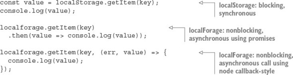
The localForage API supports both promises and Node’s error-first callback convention.

Listing 8.28. Comparison of getting data with localStorage vs. localForage

Under the hood, localForage utilizes the best storage mechanism available in the current browser environment. If IndexedDB is available, localForage will use that. Otherwise, it’ll try to fall back to WebSQL or even using web storage if required. You can configure the order in which the stores will be tried and even blacklist certain options:

Unlike localStorage, localForage isn’t limited to storing just strings. It supports most JavaScript primitives such as arrays and objects, as well as binary data types: Typed-Arrays, ArrayBuffers, and Blobs. Note that IndexedDB is the only back end that can store binary data natively: the WebSQL and localStorage back ends will incur marshalling overheads:

Promise.all([
  localforage.setItem('number', 3),
  localforage.setItem('object', { key: 'value' }),
  localforage.setItem('typedarray', new Uint32Array([1,2,3]))
]);

Mirroring the web storage APIs makes localForage intuitive to use, while also overcoming many of the shortcomings and compatibility issues when trying to store data in the browser.

8.15. Hosted storage

Hosted storage is another tactic you can use to avoid managing your own server-side storage. Hosted infrastructure services such as those provided by Amazon Web Services (AWS) are often considered as only a scaling and performance optimization, but smart usage of hosted services early on can save a lot of time implementing unnecessary infrastructure poorly.

Many, if not all, of the databases listed in this chapter have a hosted offering. Hosted services allow you to try tools quickly and even deploy publicly accessible production applications without the hassles of setting up your own database hosting. But hosting your own is becoming increasingly easy. Many cloud services provide prebuilt server images, loaded with all the right software and configurations needed to run a machine hosting the database of your choosing.

8.15.1. Simple Storage Service

Amazon Simple Storage Service (S3) is a remote file-hosting service provided as a part of the popular AWS suite. S3 is a cost-effective means of storing and hosting network-accessible files. It’s a filesystem in the cloud. Using RESTful HTTP calls, files can be uploaded into buckets, along with up to 2 KB of metadata. Bucket contents can then be accessed via HTTP GET or the BitTorrent protocol.

Buckets and their contents can be configured with various permissions, including time-based access. You can also specify a time to live (TTL) on bucket contents themselves, after which they’ll become inaccessible and be removed from your bucket. It’s easy to promote your S3 data up to a content delivery network (CDN). AWS provides the CloudFront CDN, which can be easily connected to your files and will be accessible with low latency from around the world.

Not all data needs to be or should be stored in a database. Are there components of your data that could be treated as files? After you’ve generated the results of an expensive calculation for a user, perhaps you can push those results up to S3 then forever step out of the way.

A common and obvious use for S3 is the hosting of user-uploaded assets such as images. Uploaded assets live in a temporary directory on the application machine, processed by using a tool such as ImageMagick to reduce the file size, and then uploaded to S3 for hosting to web browsers. This process can be simplified even further by streaming uploads directly to S3, where they can trigger further processing. The client-side applications can also upload to S3 directly. Some more developer-centric services even opt for providing absolutely zero storage, requiring users to provide access tokens so the application can use their S3 buckets.

S3 isn’t limited to the storage of images

S3 can be used to store any type of file, up to 5 terabytes in size, of any format. S3 works best for large blobs of data that change infrequently and need to be accessed as a single atom.

Storing data in S3 steps around the complications and complexity of setting up and maintaining a server for the hosting and storage of files. It’s great for instances where writes are infrequent, large chunks of data need to be accessed as a single atom, and there are many reads and potentially many read locations.

8.16. Which database?

In this chapter, we’ve covered just a few of the many databases commonly used in Node applications. Successful applications can be and have been built using any of these databases. Within a single application, there’s not always one ideal data storage solution; there’s no silver bullet. Each database presents its own unique set of trade-offs, and it’s up to the developer to evaluate which trade-offs make sense for the current state of the project. A hybrid of technologies is frequently the most appropriate.

Rather than asking, “What database should I use?” you could be asking, “How far can I go without using a database at all?” How much of your project can you build with the fewest long-lasting decisions? It’s often best to defer decisions; you’ll always be able to make a better decision later, when you have more information.

8.17. Summary

• Both relational and NoSQL databases can be used with Node.
• The simple pg Node module is great for working with the SQL language.
• The Knex module allows you to use several databases with Node.
• ACID is a set of properties for database transactions and ensures safety.
• MongoDB is a NoSQL database that uses JavaScript.
• Redis is a data-structure store that can be used as a database and cache.
• LevelDB is a fast key/value store by Google that maps from strings to values.
• LevelDB is a modular database.
• Web-based storage, including localForage and localStorage, can be used to save data in browsers.
• Storage services, such as Amazon S3, can be used to persist data to cloud providers.