Table of Contents for
Programming Quantum Computers
 Programming Quantum Computers
Published by
O'Reilly Media, Inc., 2019
Programming Quantum Computers
Published by
O'Reilly Media, Inc., 2019
Chapter 3. Multiple Qubits
As useful as qubits are individually, they are much more useful (and more intriguing) in groups. We’ve already seen in Chapter 2 how the distinctly quantum phenomenon of superposition introduces new parameters that we can use for computation (magnitude and phase). But when our QPU has access to more than one qubit, we can also start to make use of a second powerful quantum phenomenon known as quantum entanglement. Quantum entanglement is a very particular kind of powerful interaction between qubits. In this chapter, we’ll see entanglement in action, and develop complex and sophisticated ways to utilize it.
But before we can explore some of the abilities groups of multiple qubits have to offer, we’ll need ways to visualize them.
Circle notation for multi-qubit registers
How can we extend our circle notation to multiple qubits? If we were only ever interested in qubits that didn’t interact with one another, then we could simply employ the representation we used for a single qubits, but multiple times - using a pair of circles for the ∣0〉 and ∣1〉 states of each qubit. Although this naive representation allows us to describe a superposition of any one individual qubit, there’s are ways we might superpose groups of qubits that it cannot represent (as we’ll see below).
So how else could we represent the state of a register of multiple qubits? Just as is the case with conventional bits, a register of N qubits can be used to represent one of  different values. For example, a register of three qubits, having qubits in the states ∣0〉∣1〉∣1〉 can represent a decimal value of 3. When talking about multi-qubit registers, we’ll often describe the decimal value that the register represents in the same quantum notation that we used for a single qubit. So whereas a single qubit can be in the states ∣0〉 and ∣1〉, a two-qubit register has possible states ∣0〉, ∣1〉, ∣2〉 and ∣3〉. Making use of the quantum nature of our qubits we can also create superpositions of these different values. This being the case, to represent N qubits, let’s use a separate circle for each of the 2N different values that an N-bit number can assume.
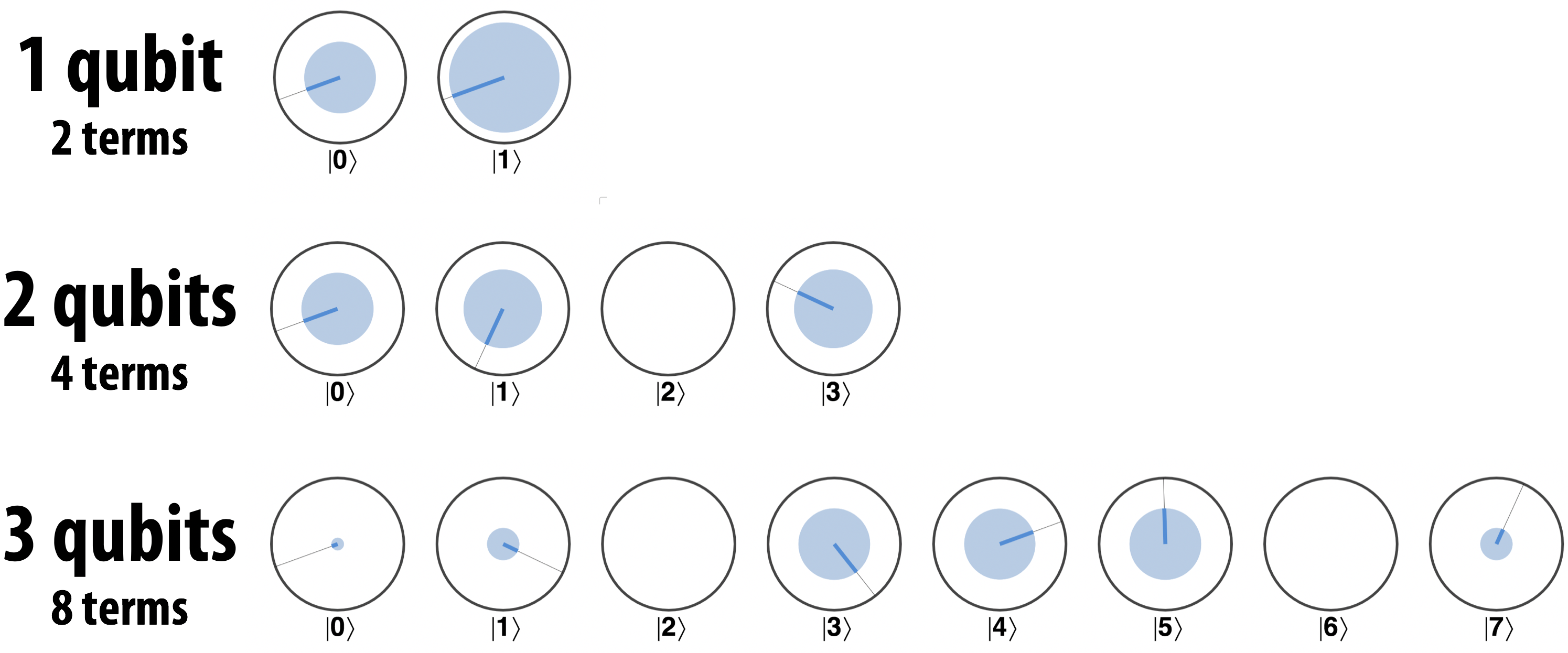
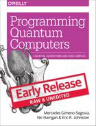
Figure 3-1. Circle notation for various numbers of multiple qubits
In Figure 3-1, we see the familiar 2-circle ∣0〉, ∣1〉 representation for a single qubit. For two qubits we have circles for ∣0〉, ∣1〉, ∣2〉, ∣3〉. This is not “one pair of terms per qubit”; instead, it is one term for each possible two-bit number you may get by reading these qubits. For four qubits, the terms are ∣0〉 … ∣7〉. As shown above, this means that we can now associate a magnitude and relative phase with each of these 2N values. In the case of the 3-qubit example, the magnitude of each of the circles represents the probability that a specific 3-bit value (0-7) will be observed when all three qubits are read.
You may be wondering what such a superposition of a registers value looks like in terms of the states of the individual qubits making up the register. In some cases we can easily see what the individual qubit states must be. For example, in Figure 3-2 the three-qubit register superposition of the states ∣0〉, ∣2〉, ∣4〉 and ∣6〉 can easily be expressed in terms of each individual qubit’s state.
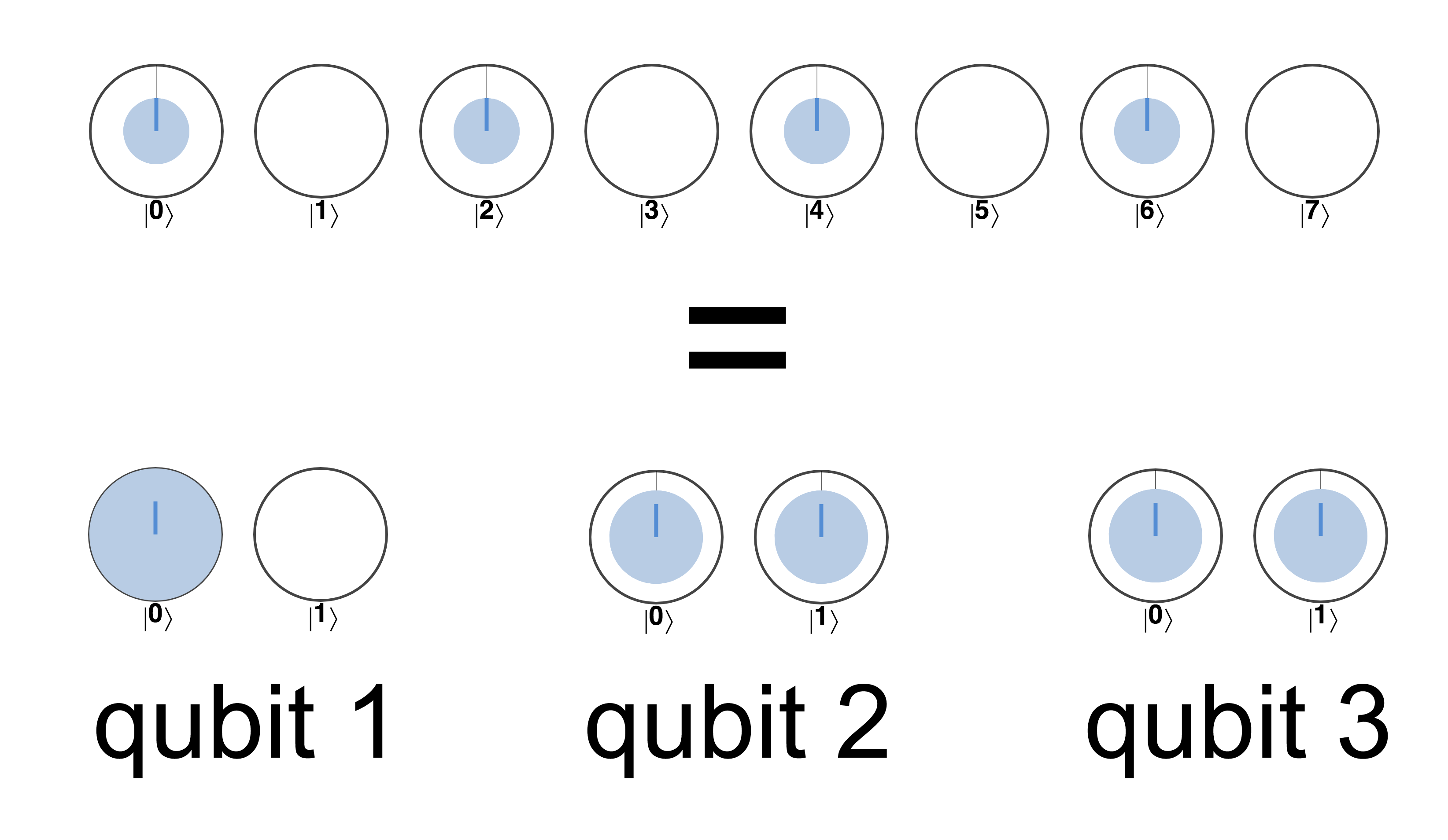
Figure 3-2. Some multi-qubit quantum states can be understood in terms of single qubit states
In fact, this multiqubit state can be cenerated simply using two single-qubit HAD operations, as shown by the following code snippet:
Tip
Example 3-1 introduces some new QCEngine notation. When dealing with multi-qubit registers we’ll have a lot of qubits to keep track of. The qint object allows us to label our qubits and treat them more like a standard programming variable. Once we’ve setup our register with some qubits (using qc.reset), qint.new() allows us to assign them to qint`s. The first argument to `qint.new() specifies how many qubits to assign to this qint from the stack created by qc.reset() (we’ll later find it useful to sometimes group sub-registers of qubits). The second argument takes a label that is used in the circuit visualizer. qint objects have many methods allowing us to apply QPU operations directly to a given qubit. For example, above we use qint.had().
So we can understand the multi-qubit state in Figure 3-2 in terms of its constituent qubits. But take a look at the state of a three-qubit register shown in Figure 3-3.
Figure 3-3. Quantum relationships between multiple qubits.
This represents the state of a three qubits in equal superposition of ∣0〉 and |7>. Can we visualize this state in terms of what each individual qubit is doing like we did in Figure 3-2? Since 0 and 7 are 000 and 111 in binary, we have a superposition of all three qubits being in the state ∣0〉 (∣0〉∣0〉∣0〉) and all three qubits being in state ∣1〉 (∣1〉∣1〉∣1〉)). Surprisingly, in this case, there is no way to write down circle representations for the individual qubits! Notice that for this three qubit state a readout of the qubits always results in us finding them to have the same values (with 50% probability that value will be 0, and with 50% probability it will be 1). So clearly the three qubits must, in some sense, be linked - to ensure that their outcomes are the same.
This link is the new and powerful entanglement phenomenon that we previously mentioned. Entangled states can’t be described only in terms of what the individual qubits are doing - although you’re welcome to try! The entanglement link is only describable in the configuration of the whole multi-qubit register. It also turns out to be impossible to produce entangled states from only single-qubit operations. So to explore entanglement in more detail, we’ll need to introduce multi-qubit operations, and for that we’ll need to be able to deftly apply everything we’ve learned so far to circuits containing registers of many qubits.
How many bits per qubit?
In articles about quantum computing, be wary when authors make assertions such as “…12 qubits, the equivalent of 4096 bits…”. As you have hopefully discovered already, bits and qubits are different units, and there is no straightforward conversion.
Drawing a Multi-Qubit Register
We now know how to describe the configuration of N qubits in circle notation using 2N circles, but what about drawing multi-qubit quantum circuits? Since our multi-qubit circle notation considers each qubit to take a position in a length N bit-string, it will be convenient to label each qubit according to it’s binary value.
As an example, let’s take another look at the random qubyte circuit we introduced in Chapter 2. There we simply labelled the eight qubits as qubit 1, qubit 2, etc… But here’s how that circuit looks if we properly label each qubit with the binary value it represents. Note that we follow the standard memory addressing practise of using hexadecimal:
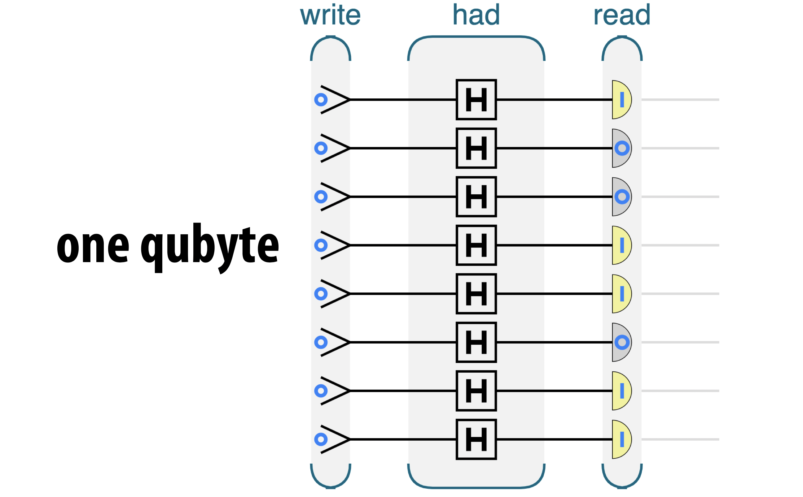
Figure 3-4. One random byte
Naming qubits
Note that in Figure 3-5 we write our qubit values in hexadecimal, using notation such as 0x1 and 0x2. This is standard programmer notation for hexadecimal values, and we’ll use this throughout the book as a very convenient notation to clarify when we’re talking about a specific qubit - even in cases when we have large numbers of them.
Single-qubit Operations in Multi-Qubit Registers
Now we know how to draw circuits of multiple qubits, and how to represent them in circle notation, let’s start doing something with them. Starting with the operations we’ve already covered, what happens (in circle notation) when we apply single-qubit operations such as NOT, HAD and PHASE to a multi-qubit register? The operation is almost identical to the single-qubit case. The only difference is that the circles are operated on in certain operator pairs specific to the qubit that the operation acts on.
To identify a qubit’s operator pairs, match each circle with the one whose value differs by the qubit’s bit-value, as shown in Figure 3-5.
Once these operator pairs have been identified, the operation is performed on each pair, just as if the members of a pair were the ∣0〉 and ∣1〉 values of a single-qubit register. For a NOT operation, the circles in each pair are simply swapped as in Figure 3-5.
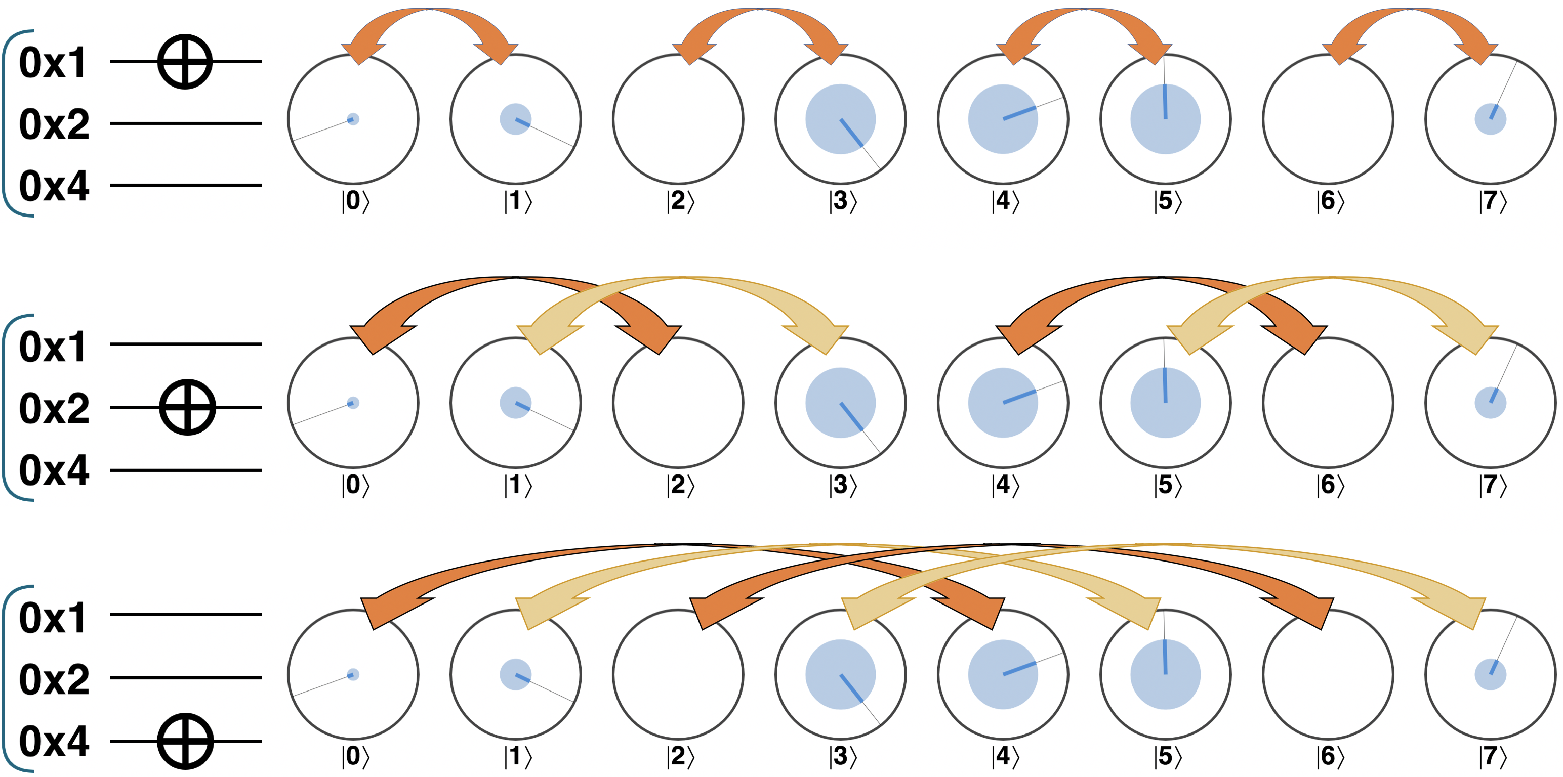
Figure 3-5. The NOT operation swaps terms in each of the qubit’s operator pairs.
For a single-qubit PHASE operation, the right-hand circle of each pair is rotated by the phase angle, as in Figure 3-6
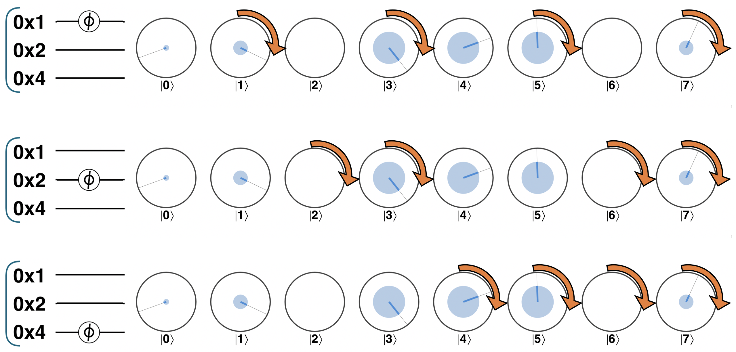
Figure 3-6. Single-qubit phase in a multi-qubit register.
Thinking in terms of operator pairs is a good way to quickly visualize the action of single-qubit operations on a register. For a deeper understanding of why this works we need to think about the effect that an operation on a given qubit has on the binary representation of the whole register. For example, the circle-swapping action of a NOT on the second qubit in Figure 3-5 corresponds to simply flipping the second bit in each term’s binary representation. Similarly, a single-qubit PHASE operation on (for example) the third qubit rotates each circle for which the third bit is 1. A single-qubit PHASE will always cause exactly half of the terms to be rotated, and which half just depends on which qubit is the target of the operation.
The same kind of reasoning helps us think about the action of any other single qubit operation on qubits from larger registers.
Reading a qubit in a multi-qubit register
What should we expect when we perform a READ operation on a single qubit from a multi-qubit register? A READ operation also functions using operator pairs. If we have a multi-qubit circle representation then we can determine the probability of obtaining a “0” outcome for one single qubit by adding the magnitudes of all of the circles on the ∣0〉 (left-hand) side of that qubits operator pairs. Similarly we can determine the probability of “1” by adding the magnitudes of all of the circles on the ∣1〉 (right-hand) side of the qubits operator pairs.
Following a READ, the state of our multi-qubit register will change to reflect which outcome occurred. All circles which do not agree with the result, will be eliminated as shown in Figure 3-7 (following this elimination, the state will also have the remaining terms ‘renormalized’ so that their magnitudes add up to 100%). Figure 3-7 below illustrates how the READ operation affects a multi-qubit register in circle notation:
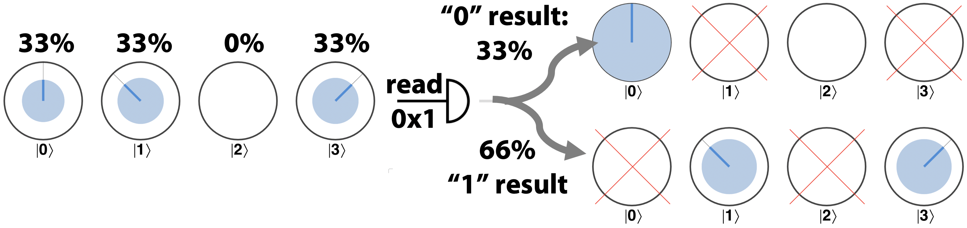
Figure 3-7. Reading one qubit in a multi-qubit register
To read more than one qubit, each single-qubit read operation can be performed individually according to this operator pair prescription.
Visualizing Larger Numbers of Qubits
Since N qubits require 2N terms (circles in circle notation), each additional qubit we might add to our QPU doubles the number of terms (or circles) we need to keep track of. As Figure 3-8 shows, the number of terms quite quickly increases to the point where our circle notation circles become vanishingly small.
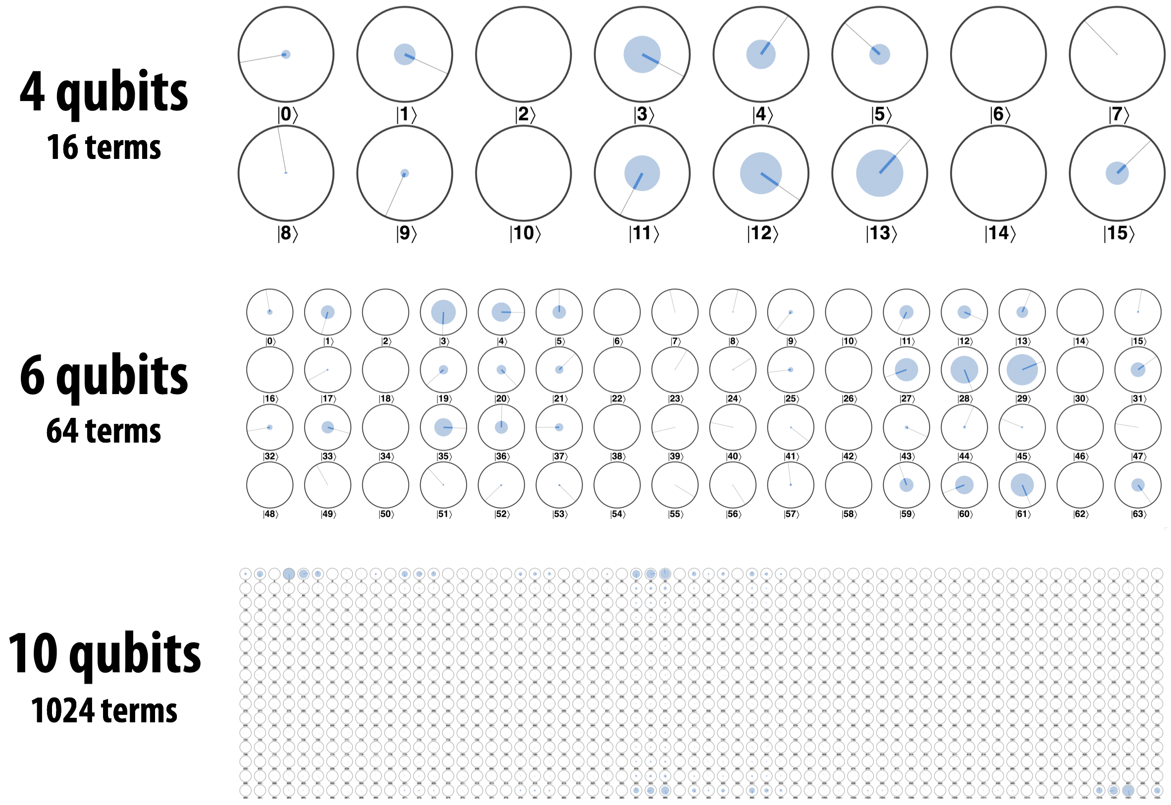
Figure 3-8. Circle notation for larger qubit counts
With so many tiny circles, the circle-notation visualization becomes useful for seeing patterns instead of individual values, and we can zoom in to any areas we want a more quantitative view of. Nevertheless, we can improve clarity in these situations by exaggerating the amplitudes, making the phase-needles bold, and also using differences in color or shading to emphasize differences in phase as shown in Figure 3-9.
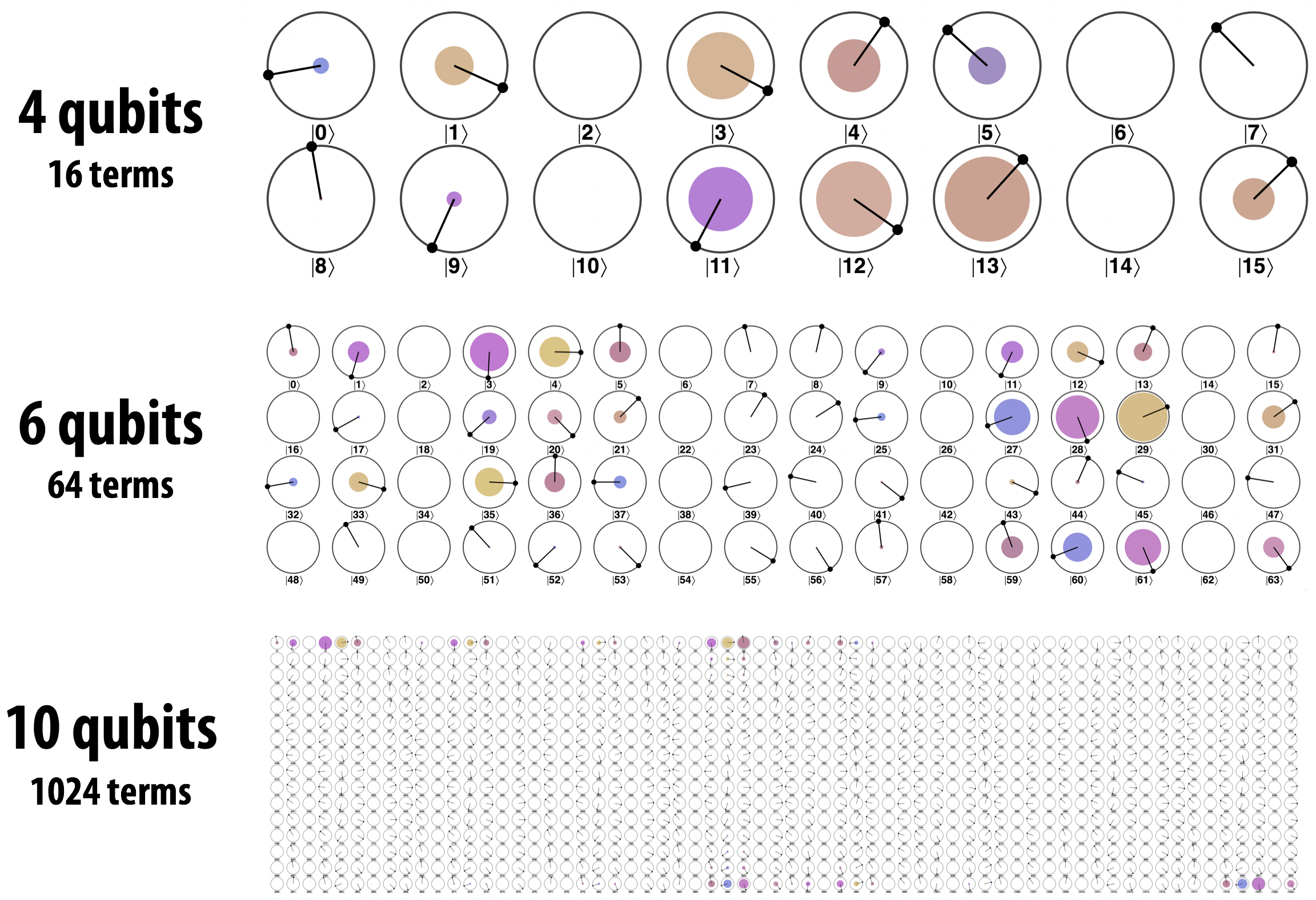
Figure 3-9. Sometimes exaggeration is warranted
In the chapters ahead, we will sometimes make use of these techniques to illustrate aspects of quantum states. But even these eyeball-hacks are only useful to a point; for a 32-qubit system there are 4,294,967,296 circles. Displaying them in a 65,536x65,536 grid of circles is too much information for most displays and eyes alike.
Tip
In your own QCEngine programs you can add the line qc_options.color_by_phase = true; to the very beginning to enable the phase coloring shown in Figure 3-9. The bold needles can also be toggled by including the line qc_options.book_render = true;.
QPU Instruction: CNOT
Now we’ve flexed our multi-qubit muscles implementing our familiar single qubit operations on larger QPU registers, it’s time to introduce some definitively multi-qubit QPU operations. By multi-qubit operations we mean ones that have mult-qubit inputs, requiring more than one qubit to operate. The first of these we’ll consider is the powerful CNOT operation. CNOT works on two qubits and can be thought of as an “if” programming construct with the following condition: “Apply the NOT operation normally to a target qubit, but only if a condition qubit has the value 1.” The circuit symbol used for CNOT shows this logic by connecting two qubits with a line. A filled dot represents the control qubit whilst a NOT symbol show the target qubit to be conditionally operated on.
The idea of using condition qubits to selectively apply actions is used in many other QPU operations, but CNOT is perhaps the most basic example. Figure 3-10 illustrates the difference between applying a NOT operation to a qubit within a register versus applying CNOT (conditioned on some other control qubit).
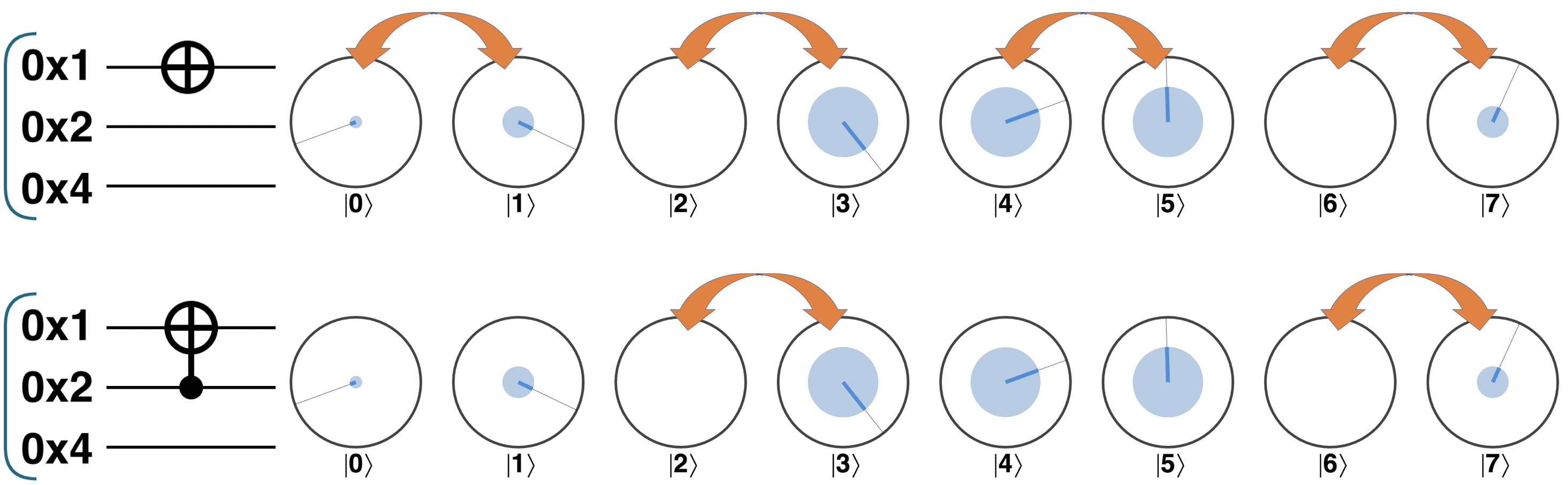
Figure 3-10. CNOT in operation
The orange arrows show which operator pairs have their circles swapped in circle notation. We can see that the essential operation of CNOT is the same as that of NOT, only more selective - applying the NOT operation only to terms whose binary representations (in this example) have a 1 in the second bit (eg: 2=010, 3=011, 6=110 and 7=111).
Reversibility: Like the NOT operation, CNOT is its own inverse; applying the CNOT operation twice will return the multi-qubit register state that we began with.
On its own there’s nothing particularly quantum about CNOT (conditional logic is of course a fundamental feature of conventional CPU’s). But armed with the conditional logic of the CNOT we can now ask an interesting and distinctly quantum question. What would happen if the control qubit of a CNOT operation is in a superposition? We can simulate this situation for a 2 qubit register using the circuit in Figure 3-11.
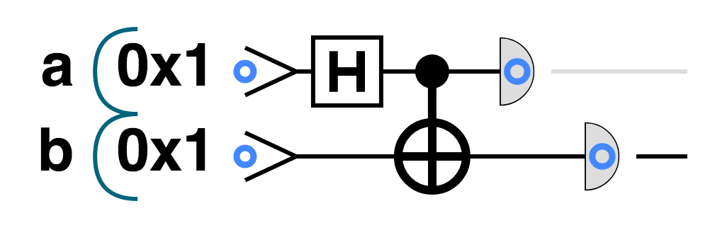
Figure 3-11. CNOT with a target qubit in superposition
Note that, for ease of reference, we’ve temporarily labeled our two qubits as a and b (rather than using hexadecimal). Starting with our register in the ∣0〉 state, let’s walk through the circuit and see what happens.
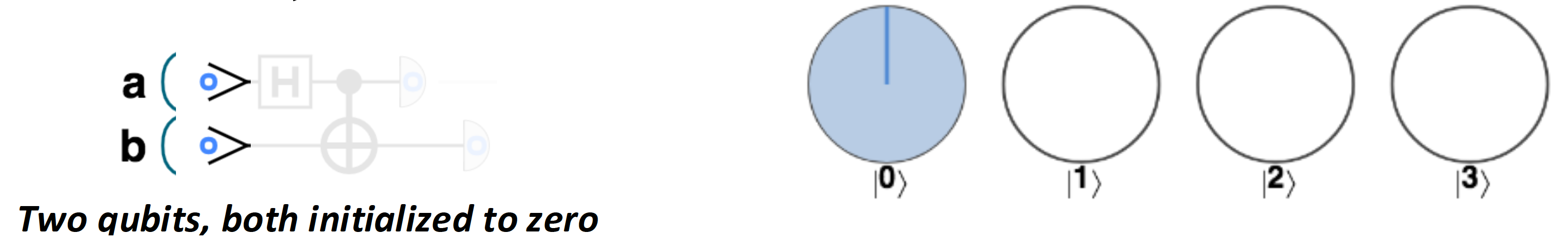
Figure 3-12. Bell Pair step 1
First we apply HAD to qubit a. Since a is the lowest weight qubit in the register, this creates a superposition of the terms ∣0〉 and ∣1〉, visualized below in circle notation:
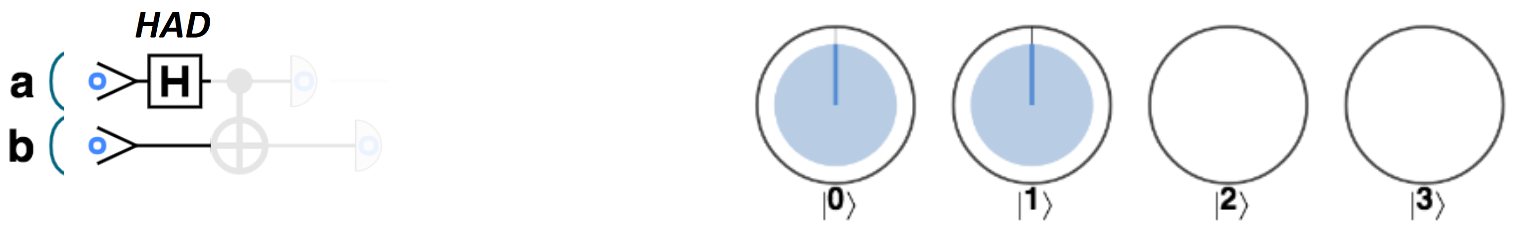
Figure 3-13. Bell Pair step 2
Next we apply the CNOT operation such that qubit b is conditionally flipped, dependent on the state of
qubit a.
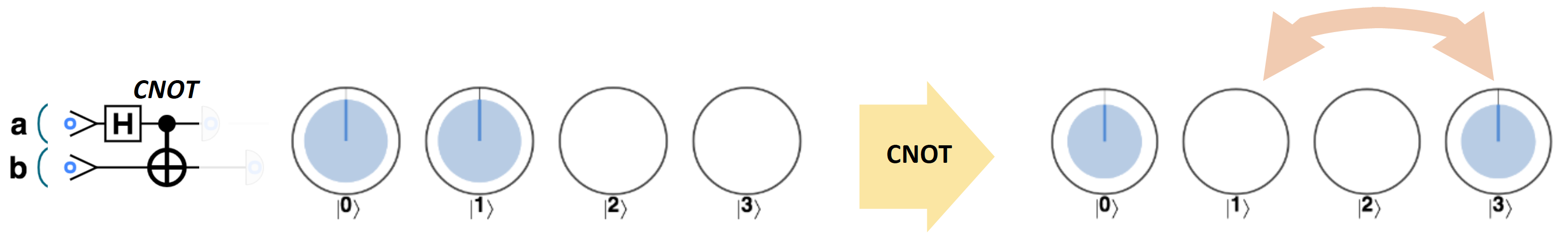
Figure 3-14. Bell Pair step 3
The result is a superposition of ∣0〉 and ∣3〉. This makes sense, since if qubit a had taken value ∣0〉 then no action would occur on b, and it would remain in the state ∣0〉 - leaving the register in a total state of ∣0〉∣0〉. However, if a had been in state ∣1〉 then a NOT would be applied to b and the register would have a value of ∣1〉∣1〉=∣3〉. Another, way to understand the CNOT’s operation in Figure 3-14 is that it simply follows the rule of changing the value of qubit b - which implies swapping the states ∣1〉 and ∣3〉 (as is shown by the orange arrow in Figure 3-14). In this case, one of these circles just so happens to be in superposition.
What we obtain in Figure 3-14 turns out to be a very powerful resource. In fact, it’s the two-qubit equivalent of the entangled state we first saw in Figure 3-3. We’ve already noted that these entangled states demonstrate a kind of interdependence between qubits - if we read out the two qubits shown in Figure 3-14, then although the outcomes will be random they will always agree (i.e. be either 00 or 11, but with 50% chance for each). And we’ve also mentioned that these states can’t be described only in terms of the individual qubits making up the register.
The one exception we made so far to our mantra of “avoid physics at all costs”, was to give a slightly deeper insight into superposition. The phenomenon of entanglement is equally important within a QPU, and so - for one final time - we’ll indulge ourselves in a few sentences of physics to give you a better feel for why entanglement is so powerful. Again, if you prefer code samples over physics insight, then you can happily skip the next couple of paragraphs without side effect.
Tip
If you want to steer clear of physics altogether then you can skip the next couple of paragraphs explaining entanglement without any ill effect.
From what we’ve seen so far, entanglement might not necessarily strike you as strange. Finding agreement between the values of bits certainly isn’t cause for concern - not even if they randomly assume correlated values. In conventional computing if two otherwise random bits are always found to agree on readout then there are two entirely rational possible explanations.
-
Some mechanism in the past has coerced their values to be equal (which we simply discover on reading them out) - what we might call a common cause. Their randomness is therefore illusory.
-
The two bits truly do randomly assume particular values at the very moment of readout, but by some method they are able to communicate with each other, to ensure they correlate.
In fact, with a bit of thought is possible to see that - for conventional bits - these are the only two ways we could explain how two bits can randomly agree.
Yet through a clever experiment, initially proposed by the great Irish physicist John Bell, it’s possible to conclusively demonstrate that entanglement allows such agreement, but without either of these two reasonable explanations being responsible! This is the sense in which you may hear it said that entanglement is a kind of distinctly quantum link between qubits that is stronger than could ever be conventionally possible. As we start programming more complex QPU applications, entanglement will begin popping up everywhere. You won’t need to explicitly think about it too hard, but it’s helpful to have a litle insight into what’s going on under the hood.
Hands-on: Using Bell Pairs for shared randomness
The entangled state we created in Figure 3-14 is commonly referred to as a Bell pair1. Let’s see a quick and easy way to put the powerful link within this state to use.
We saw in the previous chapter how simply measuring a qubit in superposition provides us with a Quantum Random Number Generator. Similarly, the reading out of a Bell pair acts like a QRNG, only now we will obtain agreeing random values on two qubits.
A surprising fact about entanglement is that the qubits involved remain entangled no matter how far apart we may move them. Thus we can easily use Bell pairs to generate correlated random bits at different locations. Such bits can be the basis for establishing secure shared randomness - something that critically underlies the modern internet.
The below code snippet shows how we can implement this prescription to generate shared randomness, by creating a Bell pair and then reading out a value from each qubit.
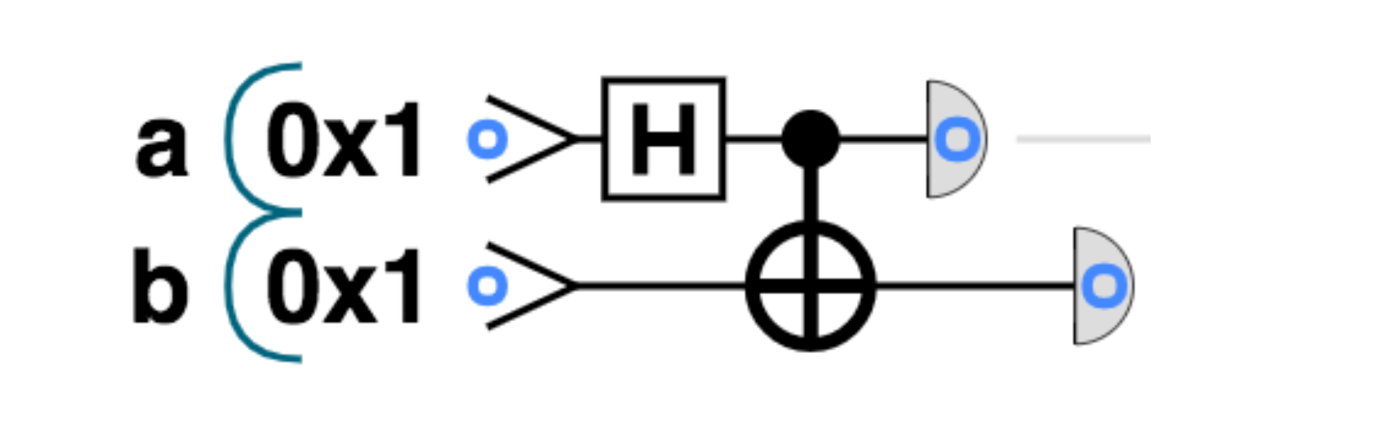
Figure 3-15. Bell Pair circuit
QPU Instruction: CPHASE and CZ
Another very common two-qubit operation is CPHASE( ). Like the CNOT operation, CPHASE employs a kind of conditional logic that can generate entanglement between qubits. Recall from Figure 3-6 that the single-qubit PHASE(
 ) operation acts on a register to rotate (by angle
  ) the ∣1〉 values in that qubits operator pairs. As CNOT did for NOT, CPHASE restricts this action on some target qubit to only occur when another control qubit assumes a value ∣1〉. Note that CPHASE only acts when its control qubit is ∣1〉, and when acting only affects target qubit states having value ∣1〉. This means that a CPHASE(
 ) applied to, say, qubits
 0x1 and 0x4 results in the rotation (by  ) of all circles for which both these two qubits have a value of 1. Because of this particular propert of the action of PHASE, CPHASE has a symmetry between its inputs not shared by CNOT. Unlike most other controlled operations, it’s irrelevant which qubit we consider to be the target and which we consider to be the control for CPHASE.
Below we compare the operation of a CPHASE between the 0x1 and 0x4 qubits with individual PHASE operations on these qubits:
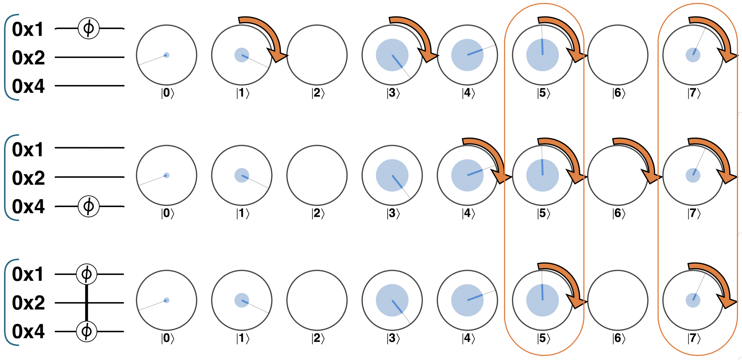
Figure 3-16. Applying CPHASE in circle notation
On their own, single-qubit PHASE operations will rotate the relative phase of half of the circles associated with a QPU register. Adding a condition cuts the number of rotated circles in half. We can also add further conditional qubits to our CPHASE, each time cutting the number of terms we act on in half again. In general, the more that we condition QPU operations, the more selective we can be with which terms of a QPU we manipulate.
QPU programs very frequently employ the CPHASE( ) operation with a phase of
 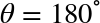 , and consequently this particular implementation of CPHASE is given its own name: CZ, along with its own simplified symbol shown in Figure 3-17. Interestingly, CZ can be constructed from HAD and CNOT very easily. Recall from Figure 2-16 that the Z operation can be made from two HAD operations and a NOT. Similarly, CZ can be made from two HAD operations and a CNOT, as shown in Figure 3-17
Figure 3-17. CZ, CPHASE and CNOT
Phase kickback
Once we start thinking about altering the phase of one QPU register conditioned on the values of qubits in some other register we can produce a surprising and useful effect known as phase kickback. Take a look at the below circuit:
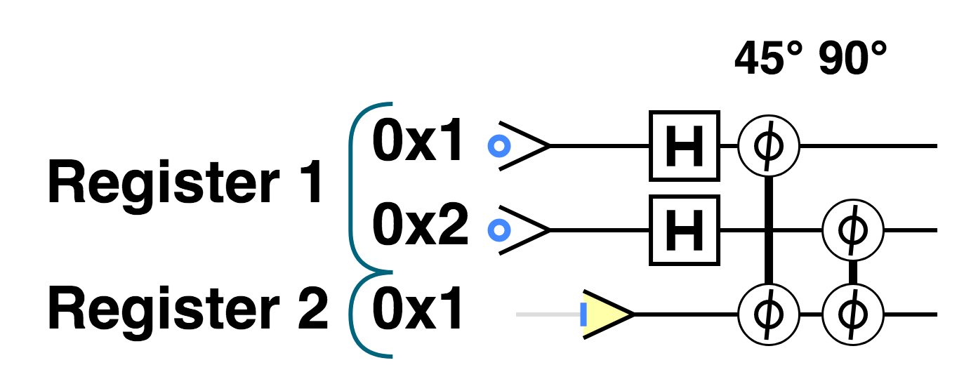
Figure 3-18. Circuit for demonstrating phase kickback trick
One way to think of this circuit is that, after placing Register 1 in a superposition of all of its  possible values, we’ve rotated the phase of
 Register 2 conditional on the values taken by Register 1`s qubits. However, looking at the resulting individual states of _both_ registers in circle notation we see that something interesting has also happened to the state of `Register 1:
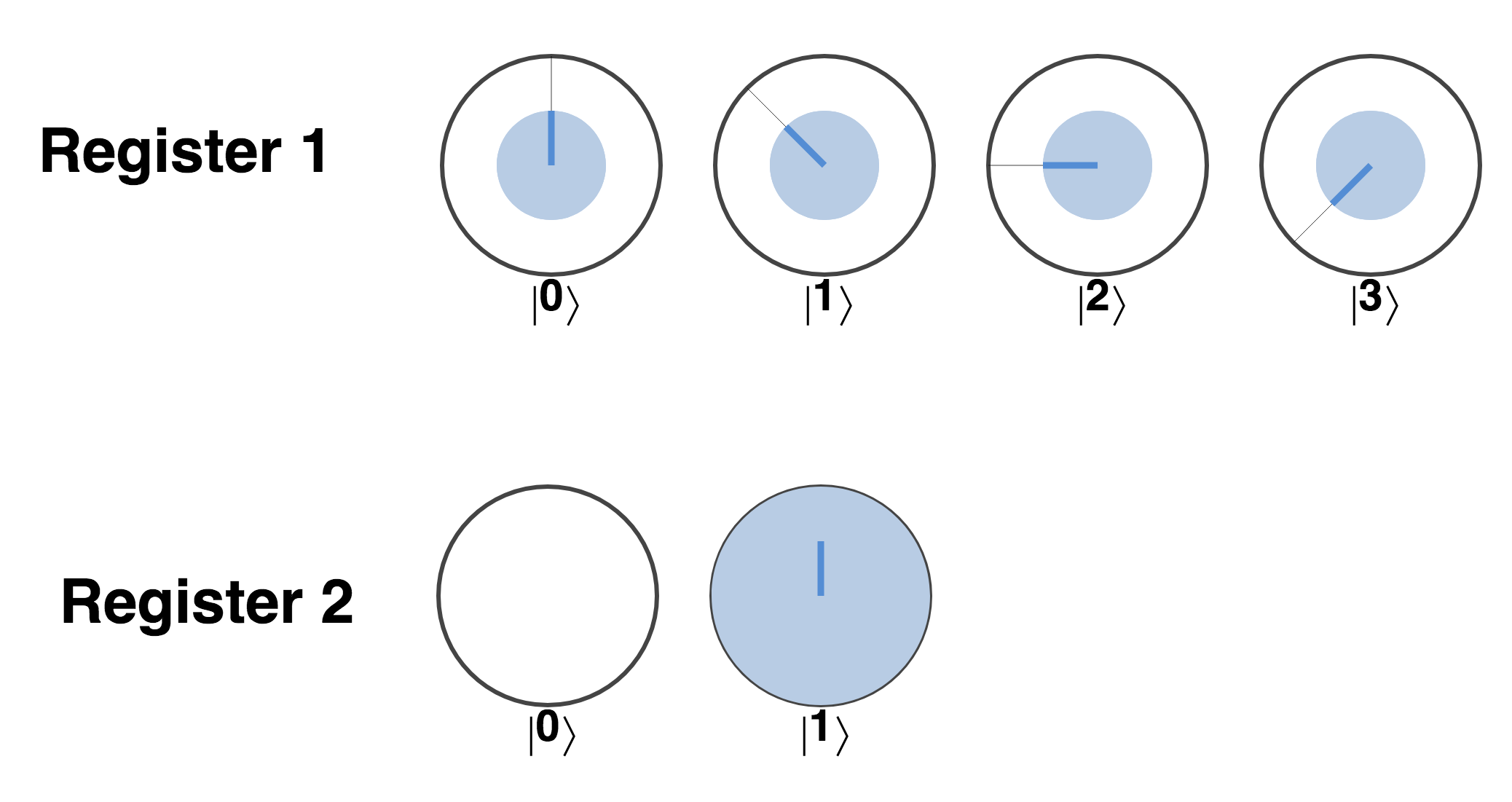
Figure 3-19. States of both registers involved in phase kickback
The phase rotations we tried to apply to the whole of the second register (conditioned on qubits from the first) have also affected different terms from the first register! More specifically, here’s what we’re seeing happen in the above circle notation representations:
-
The
 rotation we performed on
 Register 2conditioned on the lowest weight qubit fromRegister 1has also rotated every term inRegister 1for which this lowest weight qubit is activated (the ∣1〉 and ∣3〉 terms). -
The
 phase rotation conditioned on
 Register 1`s highest weight qubit has also been 'kicked-back' onto all terms in `Register 1having this qubit activated (∣2〉 and ∣3〉).
The net result that we see on Register 1 is the combination of these phase rotations that have been kicked back onto it from our intended target of Register 2.
Phase kickback is a very useful idea, as rather than seeing it as an unfortunate side-effect, we can use it to apply phase rotations to specific terms in a register (Register 1 in the above example). We can do this by performing a phase rotation on some other register conditioned on qubits from the register we really care about that chosen to specifically pick out the terms we want to rotate.
Don’t feel bad if this phase-kickback trick initially strikes you as a little mind-bending, it can take a while to get used to. The easiest way to get a feel for it is to play around with some examples to build intuition for how entanglement is linking the two registers phases. To get you started, here’s QCEngine code for reproducing the two register example we described above.
// Initialize our qubitsqc.reset(3);// Create two registersreg1=qint.new(2,'Register 1');reg2=qint.new(1,'Register 2');reg1.write(0);reg2.write(1);// Place the first register in superpositionreg1.had();// Perform phase rotations on second register,//conditioned on qubits from the firstqc.phase(45,0x1|0x4);qc.phase(90,0x2|0x4);
We’ll make use of phase-kickback in [Link to Come] to understand the inner workings of a QPU primitive, and again in <<>> to explain how a QPU circuit can help us solve systems of linear equations. The wide utility of phase kickback stems from the fact that it doesn’t only work for CPHASE operations, but any conditional operation that generates a change in phase on a register (even if the phase is a global, unREADable one). This is as good a reason as any to understand how we might construct more general conditional operations.
Constructing Any Conditional Operation
We’ve introduced CNOT and CPHASE operations, but is there such thing as a CHAD (conditional HAD), or a CRNOT (conditional RNOT)? There are, and even if a conditional version of some single qubit operation is missing from the instruction set of a particular QPU, there’s a process by which we can “convert” single qubit operations into a multi-qubit conditional ones.
The general prescription for conditioning a single qubit operation involves a little more mathematics than we want to cover here, but seeing a couple of examples will help us feel more comfortable with the idea (and also be useful to us later on). The key idea is breaking our single qubit operation into smaller steps. It turns out that it’s always possible to break a single qubit operation into a set of steps such that we can use CNOTs to conditionally undo our operation.
This is much easier to see with a simple example: suppose we are writing software for a QPU whose instruction set includes CNOT, CZ and PHASE, but no instruction to perform CPHASE. This is actually a very common case with modern QPUs, but fortunately we can easily add a CPHASE at the compiler stage.
Recall that the desired effect for a 2-qubit CPHASE is to rotate the phase for any term for which both qubits are take value ∣1〉 (in this example we consider CPHASE(90)):
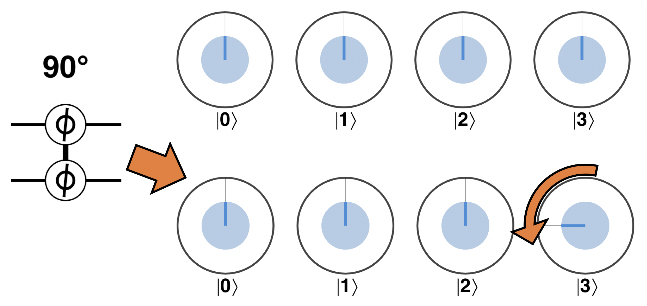
Figure 3-20. Desired operation of a CPHASE(90) operation
We can easily break down a PHASE(90) operation into smaller pieces by rotating through smaller angles. For example, PHASE(90)=PHASE(45)PHASE(45). We can also undo a rotation by rotating in the opposite direction, for example the operation PHASE(45)PHASE(-45) is the same as doing nothing to our qubit. With these facts in mind, we can construct the CPHASE(90) operation described in Figure 3-20 as follows:
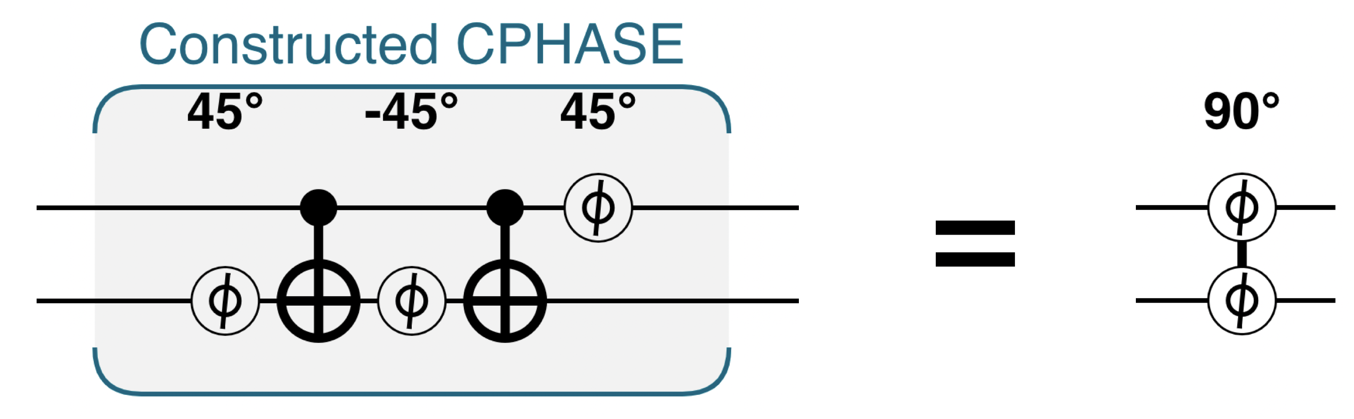
Figure 3-21. Constructing a CPHASE operation
theta=90;// Using two CNOTs and three PHASEs...qc.phase(theta/2,0x2);qc.cnot(0x2,0x1);qc.phase(-theta/2,0x2);qc.cnot(0x2,0x1);qc.phase(theta/2,0x1);// Builds the same operation as a 2-qubit CPHASEqc.phase(theta,0x1|0x2);
Following this circuit through for different possible inputs we can see how it works to only apply PHASE(90) when both qubits are 1 (an input of 11). To see this it helps to recall that PHASE has no effect on a qubit in the state ∣0〉. Alternatively, we can follow the action of Figure 3-22 using circle notation.
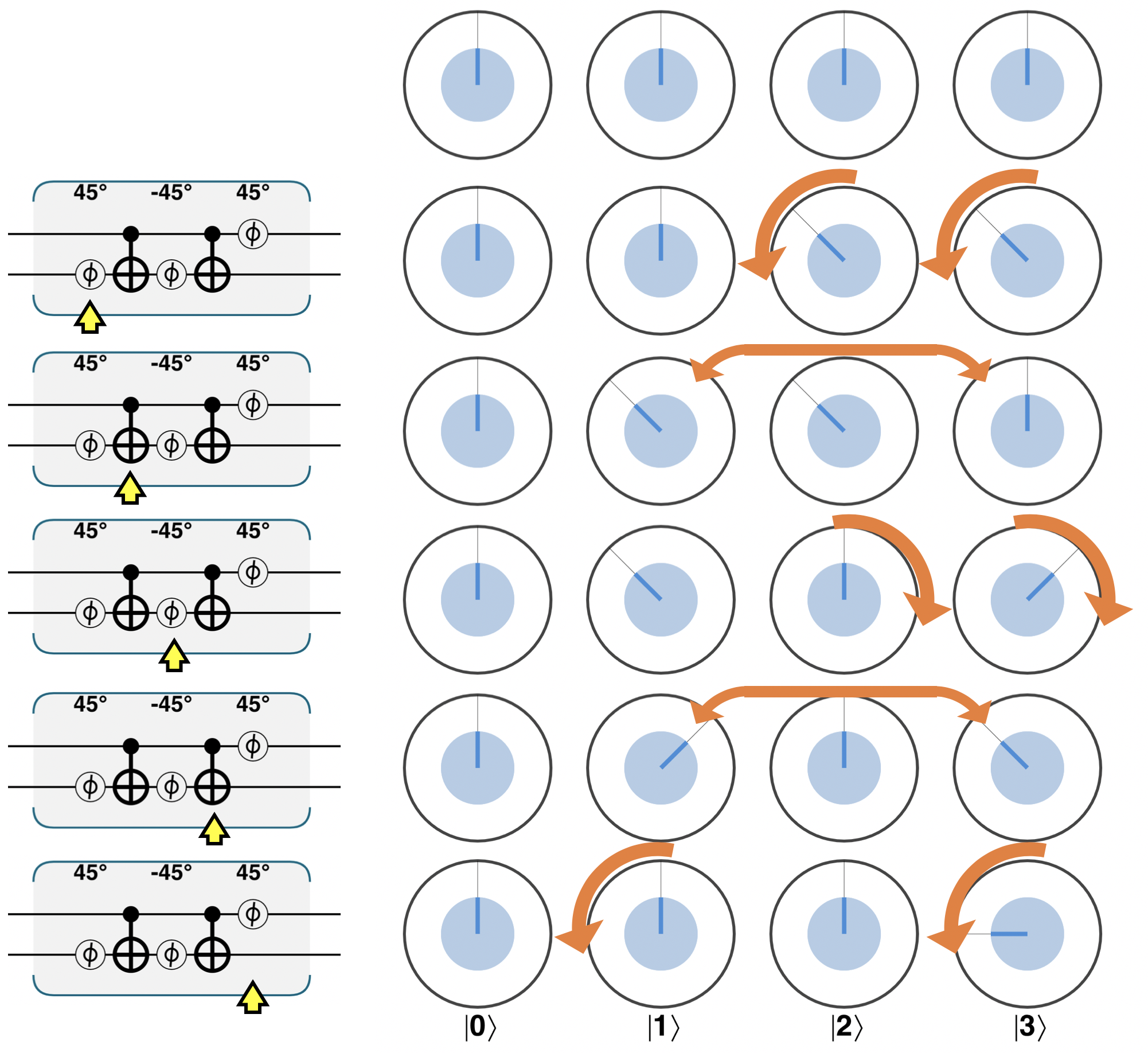
Figure 3-22. Step-by-step through the constructed CPHASE operation
Another example of conditioning a single qubit operation that will be useful to us in later chapters is ROTY…
[[ Example of conditioning ROTY to be added]]
QPU Instruction: CCNOT (Toffoli)
We’ve previously noted that multi-qubit conditional operations can be made more selective by performing operations conditioned on more than one qubit. Let’s see this in action and generalize the CNOT operation by adding multiple conditions. A CNOT with two condition qubits is commonly referred to as a CCNOT operation. The CCNOT is also sometimes called a Toffoli gate, after the eponymously titled equivalent gate from conventional computing
With each condition added, the NOT operation stays the same, but the number of operator pairs affected in the registers circle notation is reduced by half. We show this below by comparing a NOT operation on the first qubit in a three-qubit register alongside the associated CNOT and CCNOT operations.
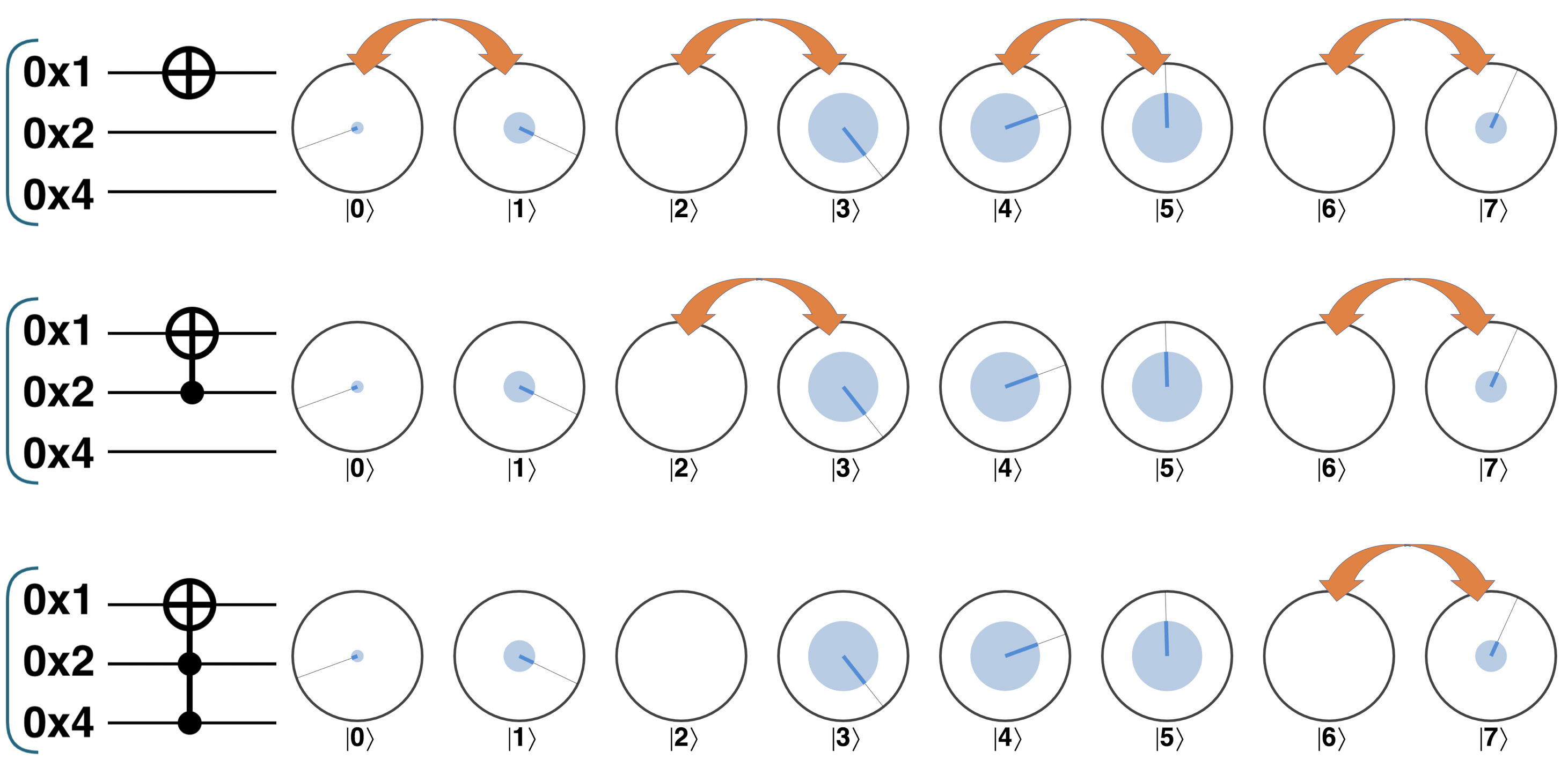
Figure 3-23. Adding conditions makes the NOT operation more selective
In a sense, a Toffoli can be interpreted as an operation implementing “if A AND B then flip C”. For performing basic logic, the Toffoli gate is arguably the single most useful QPU operation. Multiple Toffoli gates can be combined and cascaded to produce a wide variety of logic functions, as we will explore in [Link to Come].
Fan in and Fan out
The number of condition qubits which may be applied to a single CNOT-style operation on a QPU is sometimes referred to as the fan in of the QPU. The number of target qubits is referred to as the fan out.
QPU Instruction: SWAP and CSWAP
Another very common operation in quantum computation is SWAP (also called exchange), which simply exchanges two qubits. If the architecture of a QPU allows it then SWAP may be a truly fundamental operation in which the physical objects representing qubits are actually moved to swap their positions. Alternatively, a SWAP can be performed by exchanging the information contained in two qubits (rather than the qubits themselves) using three CNOT operations, as shown in Figure 3-24.
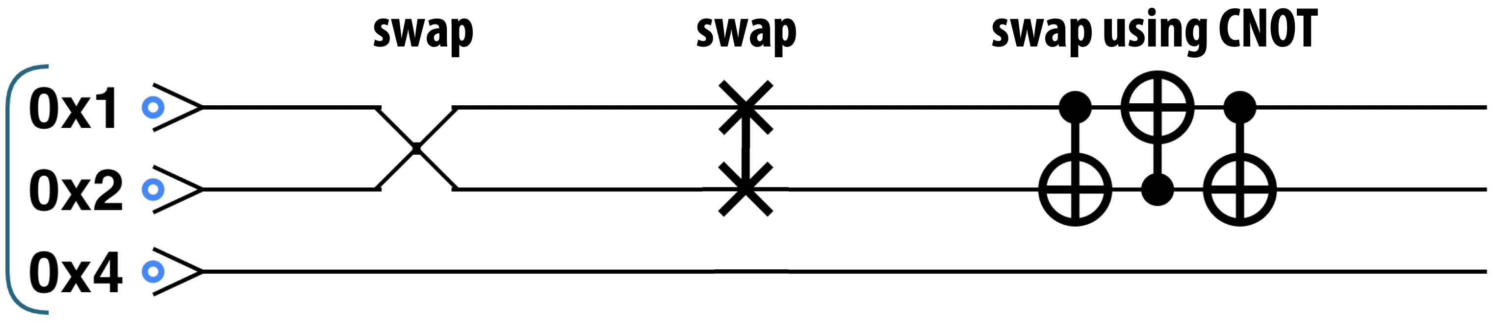
Figure 3-24. Swap can be made from CNOT operations
A digital parallel
In this book we have two ways to indicate swap operations. In the general case we use a pair of connected X’s. When the swapped qubits are adjacent to one another, it is often simpler and more intuitive to cross the qubit lines. The operation is identical in both cases.
You may be wondering why SWAP is a useful operation. Why not simply re-name our qubits instead? On a QPU, SWAP comes into its own when we consider generalizing it to a conditional operation called CSWAP, or conditional exchange. CSWAP can be implemented using three Toffoli gates, as shown in Figure 3-25.
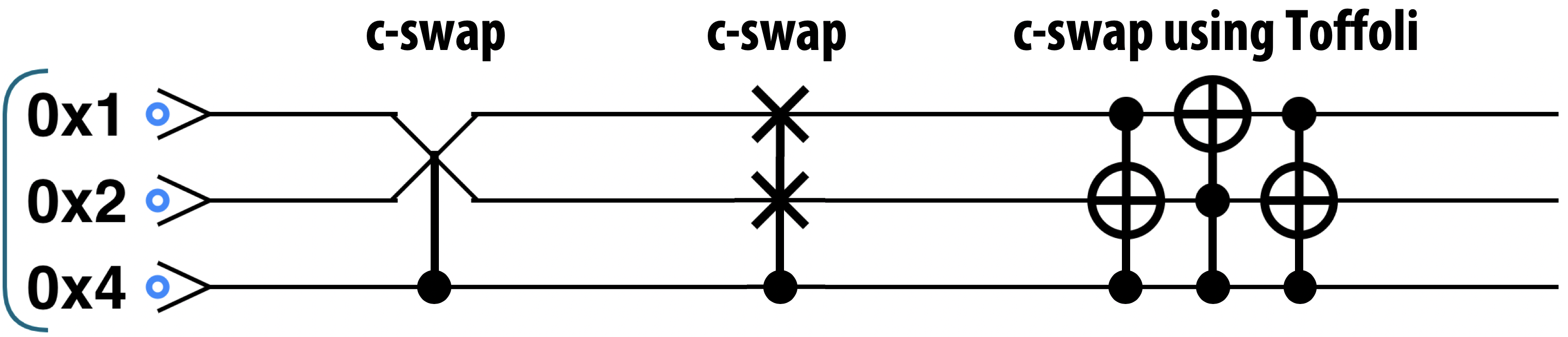
Figure 3-25. CSWAP constructed from Toffoli gates
If the condition qubit for a CSWAP operation is in superposition then we end up with a superposition of our two qubits being exchanged, and also being not exchanged. In [Link to Come] and [Link to Come], we’ll see how this feature of CSWAP allows us to perform multiplication-by-2 in quantum superposition.
Hands-on: Remote-controlled randomness
Armed with multi-qubit operations we’re now in a position to start making use of the power of quantum entanglement. We can explore some interesting and non-obvious properties of entanglement using a small QPU program for remote controlled random number generation. This program will generate two qubits, such that reading out one instantly affects the probabilities for obtaining a random bit read out from the other. Moreover, this effect occurs over any distance of space or time. This seemingly impossible task, enabled by a QPU, is surprisingly simple to implement.
Here’s how the remote control will work: We will manipulate a pair of qubits such that reading one qubit (either one) returns a 50/50 random bit which tells you the “modified” probability of the other. If the result is 0, then the other qubit will have 15% probability of being 1. Otherwise, if the qubit you read returns 1, then the other one will have 85% probability of being 1.
The sample code in Example 3-3 shows how to implement this remote controlled random number generator. As in Example 3-1 we make use of the QCEngine qint object to be able to properly address different qubits directly as objects:
We can follow the effect of each operation within this circuit in circle notation:
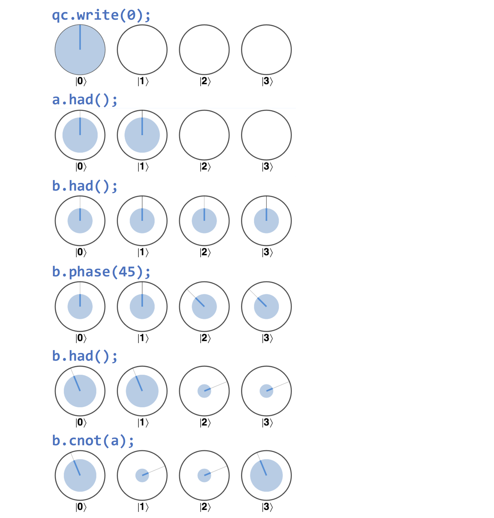
Figure 3-26. The remote-random sample, step by step
After these steps are completed we’re left with an entangled state of the two qubits shown at the end of Figure 3-26 - for which we have amplitudes in each possible state ∣0〉, ∣1〉, ∣2〉 and ∣3〉.
Let’s consider what would happen if we prepare this state and then read out qubit a. If qubit a were read out to have value 0 (as it will with 50% probability), then only the circles compatible with this state of affairs would remain. These are the terms for ∣0〉∣0〉 = ∣0〉 and ∣1〉∣0〉 = ∣2〉, and so the state of the two qubits becomes the following:
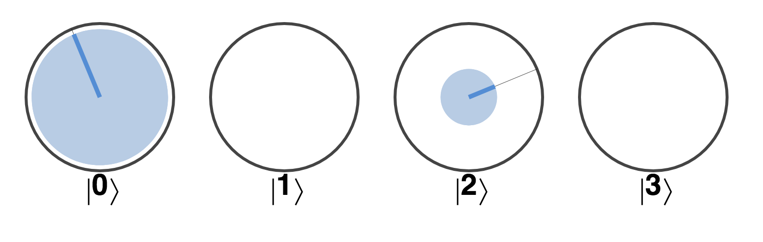
Figure 3-27. The state of one qubit in the remote control after the other is READ to be 0.
The two terms in this state have non-zero probabilities, both for obtaining 0 and for obtaining 1 when reading out qubit +b+. In particular, qubit a has 70%/30% probabilities of reading out 0/1:
However, suppose that our initial measurement on qubit a had yielded 1 (which also occurs with 50% probability). Then only the ∣0〉∣1〉=∣1〉 and ∣1〉∣1〉=∣3〉 terms will remain after the readout:
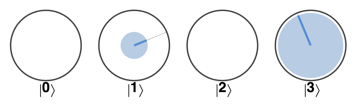
Figure 3-28. The state of one qubit in the remote control after the other is READ to be 1.
And the probabilities for reading out the 0/1 outcomes on qubit b are now 30%/70%.
Note that although we were able to change the probability distribution of readout values for qubit b instantaneously, we’re unable to do so with any intent - we can’t choose whether to cause the 70%/30% or the 30%/70% distribution - since the outcome we get when measuring qubit a is obtained randomly. It’s a good job too, since if we could make this change deterministically then we could send information instantaneously using entanglement - i.e. faster than light. Although sending signals faster than light sounds like fun, were this possible, bad things would happen2. In fact one of the strangest things about entanglement is that although it allows us to change the states of qubits instantaneously across arbitrary distances, it always does so in such way that we can never use the effect to send intelligible, pre-determined information. It would seem that the universe isn’t a big fan of sci-fi.
Conclusions
We’ve seen how single and multi-qubit operations can allow us to manipulate the properties of superposition and entanglement in the qubits of a QPU. With these operations at our disposal we’re ready to see how they can really allow us compute with a QPU in new and powerful ways. In [Link to Come] we’ll see how fundamental digital logic can be re-imagined within a QPU, but first in the next chapter we take a hands-on exploration of quantum teleportation. Not only is quantum teleportation a fundamental component of many quantum applications, but exploring it will also put to the test everything we’ve learned so far about describing and manipulating registers of qubits.
1 This, along with several other states carry that name because they were in fact the states that John Bell used in his proposed experiment for demonstrating the inexplicable nature of the correlations in entangled states
2 Sending-information-back-in-time-causality-violating kinds of bad things. The venerated work of Dr Emmett Brown attests to the dangers of such hijinks.