Table of Contents for
Programming Quantum Computers
 Programming Quantum Computers
Published by
O'Reilly Media, Inc., 2019
Programming Quantum Computers
Published by
O'Reilly Media, Inc., 2019
Chapter 1. Introduction
Quantum computers are no longer theoretical devices.
The authors of this book believe that the best uses for a new technology are not necessarily discovered by its inventors, but by domain experts experimenting with it as a new tool for their work. Discovering new applications for quantum computing means making tools accessible to these experts. With that in mind, this book is a hands-on programmer’s guide to using quantum computing technology.
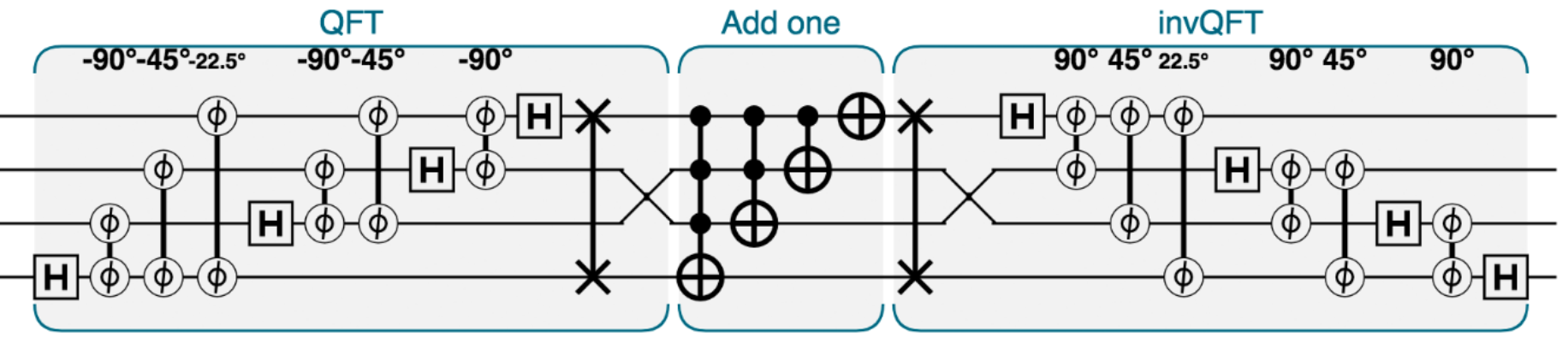
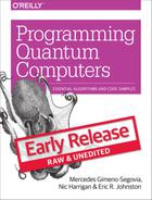
Figure 1-1. Quantum logic can look a bit like sheet music
Whether you’re an expert in software engineering, computer graphics, data science, or just a curious computerphile, this book is designed to let you learn how the power of quantum computing might be relevant to you, by actually starting to use it. In the chapters ahead, you will become familiar with symbols such as those in Figure 1-1, and the code used in applying them to problems you care about.
To facilitate this, the following chapters do not contain thorough explanations of quantum physics (the laws underlying quantum computing) or even quantum information theory (how those laws talk about processing information). Instead, they provide working examples demonstrating capabilities of this exciting new technology. Most importantly, the code we present for these examples can be tweaked and adapted. This allows you to learn from them in the most effective way possible - by being hands-on and trying things out. Along the way, core concepts are explained as they are used, and only in so far as they build an intuition for writing quantum programs.
While quantum computing technologies span a very wide range of applications such as quantum chemistry and physical simulation, this book will focus on computational primitives.
Our humble hope is that interested readers might be able to wield these insights to apply and augment applications of quantum computing in fields that physicists may not even have heard of. Admittedly, hoping to help spark a quantum revolution isn’t that humble, but it’s definitely exciting to be a pioneer.
Required background
The physics underlying the qubits of quantum computing is full of dense mathematics. But then so is the physics underlying the transistor, and yet learning C++ needn’t involve a single physics equation. In this book we take a similarly programmer-centric approach, circumventing any significant mathematical background. That said, here is a short list of background knowledge that may be helpful in digesting the new concepts that we introduce:
-
Familiarity with programming control structures (
if,while, etc.). JavaScript is used in this book to provide lightweight access to samples which can be run online. If you’re new to JavaScript but have some prior programming experience then the level of background you need could likely be picked up in less than an hour. For a more thorough introduction to JavaScript see [Learning Javascript](http://shop.oreilly.com/product/0636920035534.do). -
Occasionally we will employ some relevant programmer-level mathematics, such as:
-
An understanding of using mathematical functions.
-
Familiarity with trigonometric functions.
-
Comfort manipulating binary numbers and converting between binary and decimal representations.
-
-
A very elementary understanding of how to assess the computational complexity of an algorithm (i.e. big-o notation).
One part of the book that reaches beyond these requirements is [Link to Come] - where we survey a number of applications of quantum computing to machine learning. Due to space constraints our survey gives only very cursory introductions to each machine learning application before showing how a quantum computer can provide an advantage. Although we intend the content to be understandable to a general reader, those wishing to really experiment with these applications will require a bit more of a machine learning background (for any reader interested in developing this, we provide some introductory references in ???).
This book is about programming (not building, nor researching) quantum computers, which is why we can do without advanced mathematics and quantum theory. However, for those interested in exploring the more academic literature on quantum computing, ??? provides some good initial references and shows how you can begin to link the concepts we introduce to the mathematical notations commonly used by the quantum computing research community.
What is a QPU?
Despite its ubiquity, the term “Quantum Computer” can be a bit misleading. It conjures images of an entirely new kind of machine, probably having some kind of glowing liquid keyboard and trans-dimensional display - one that supplants all existing computing software with a futuristic alternative.
At the time of writing this is a common, albeit huge, misconception. The promise of quantum computers stems not from them being a conventional computer killer, but rather from their ability to dramatically extend the kind of problems that are tractable within computing. There are some specific, yet important, computational problems that are easily calculable on a quantum computer, but that would quite literally be impossible on any conceivable standard computing device that we could ever hope to build1.
But crucially, these kind of speedups have only been seen for certain problems (many of which we later elucidate on), and although it is anticipated that more will be discovered, it’s highly unlikely that it would ever make sense to run all computations on a quantum computer. For most of the tasks taking up your laptop’s clock-cycles a quantum computer would perform no better.
In other words - from the programmer’s point of view - a quantum computer is really a co-processor. In the past, computers have used a wide variety of co-processors, each suited to their own specialties, such as floating-point arithmetic, signal processing, and real-time graphics. With this in mind, we will use the term QPU (Quantum Processing Unit) to refer to the device on which our code samples run. We feel this reinforces the important context within which quantum computing should be placed.
As with other co-processors such as the GPU (Graphics Processing Unit), programming for a QPU involves the programmer writing code which will primarily run on the CPU of a normal computer. The CPU issues the QPU co-processor commands only to initiate tasks suited to its capabilities.
A Hands-on Approach
The hands-on samples we present form the backbone of this book. But at the time of writing a full-blown general purpose QPU does not exist - so how can you hope to ever run the code that we present? Fortunately (and excitingly), even in 2019 a few prototype QPUs are currently available from companies such as IBM, and can be accessed on the cloud. Furthermore, for smaller problems it’s possible to simulate the behavior of a QPU on conventional computing hardware. Although simulating larger QPU programs becomes impossible, for smaller code snippets it’s a much more convenient way to learn how we might control an actual QPU. The code samples in this book are compatible with both of these scenarios, and will remain both usable and pedagogical even as more sophisticated QPUs become available.
To ensure that our code samples are widely employable we provide them, whenever possible, in each of the following languages:
-
QASM: QASM is a quantum assembly language, which can run directly on hardware and simulators available from IBM, and is provided online for free public use.
-
Python: Qiskit is a free and open source Python library for quantum computation. Programs can be run in simulation as well as on IBM’s more advanced hardware.
-
JavaScript: QCEngine is a free online quantum computation simulator, allowing users to run samples in a browser, with no software installation at all. This simulator was developed by the authors, initially for their own use and now as a companion for this book. QCEngine is especially useful for us, both because it can be run without the need to download any software, and also because it incorporates the circle notation that we use as a visualization tool throughout the book.
There are many other QC simulators, libraries, and systems available. A list of links to several well-supported systems is available at [http://oreilly.machinelevel.com](http://oreilly.machinelevel.com). The three primary platforms chosen for the book represent a balance between ease-of-reading and ability to run on actual hardware available at the time of publication.
To prevent code samples from overwhelming the text, we provide samples only in JavaScript for QCEngine. This simulation engine has the advantages of being easily available online, very fast, and tailored to our approach. Full implementations of the books code samples in the other languages can be found online at [oreilly.machinelevel.com](http://oreilly.machinelevel.com).
It’s worth noting that the quantum languages we include are by no means an exhaustive list of all those available at the time of writing. While the syntax may differ, most quantum languages share the common structure and operations of the QPU. The intuitions and core concepts built by this book can readily be applied to other existing (and future) quantum programming languages.
A QCEngine primer
Since we’ll use QCEngine throughout the book, it’s worth spending a little time to see how to navigate the simulator - which may be found at http::oreilly.machinelevel.com (TODO: Finalize the URL), along with more detail its use.
Running code
The QCEngine web interface shown in Figure 1-2 allows you to easily produce the various visualizations we rely on throughout the book to get to grips with the unintuitive nature of qubits. With zero install and minimal friction, you can create these visualizations simply by entering code into the QCEngine code editor:
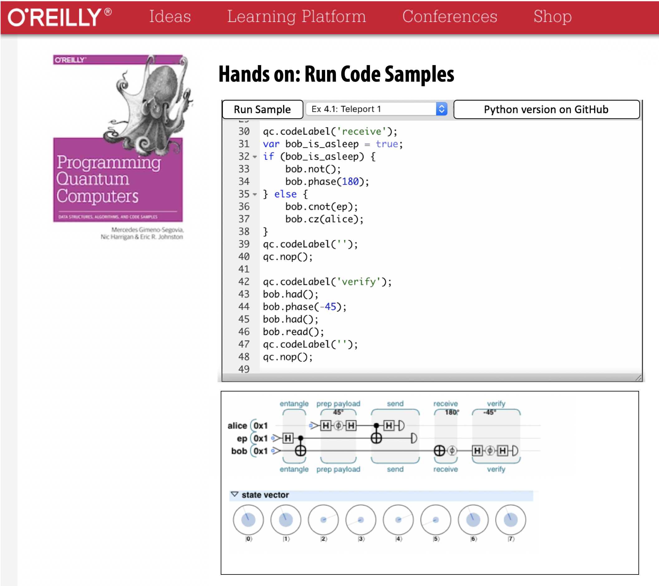
Figure 1-2. The QCEngine UI
You can also find the code samples from the book already online. To run one as-is, select it from the list at the top of the editor and click Run Sample in order to execute the code using the QCEngine. The quantum simulation will then run locally on your machine.
After clicking the Run Sample button, some new interactive UI elements will appear for visualizing the results of running your code:
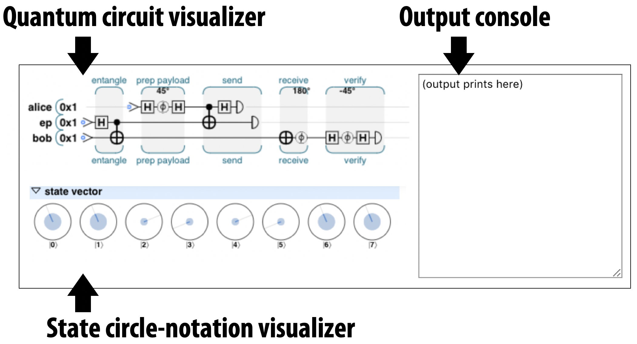
Figure 1-3. QCEngine UI elements for visualizing QPU results
Circuit visualizer: This element presents a visual representation of the circuit that your code represents. We’ll introduce the symbols used in these circuits in Chapter 2 and Chapter 3. As we describe below, this view can also be used to interactively step through the program.
State circle-notation visualizer: This displays the so-called circle-notation visualization of qubits in the QPU (or simulator) that’s running your code. We explain how to read and use this notation in Chapter 2.
QCEngine output console: This is where any text appears that may have been printed from within your code (i.e. for debugging) using the qc.print() command. Anything printed with the standard JavaScript console.log() function will still go to your web browser’s JavaScript console. As an example, if you add qc.print("No cat puns allowed"); to the end of the default QCEngine code snippet and click Run Sample again, then you should see this text in the output console.
Debugging code
Debugging QPU programs can be tough. As each line of code executes, the configuration of qubits inside the QPU changes, and quite often the easiest way to understand what a program is doing is to slowly step through it, inspecting a qubit visualization at each step. Hovering your mouse over the circuit visualizer, you should see a vertical orange line appear at a fixed position and a gray vertical line wherever in the circuit your cursor happens to be. The orange line shows which position in the circuit (and therefore the code) the circle notation visualizer currently represents. By default this is the end of the program, but by clicking on other parts of the circuit, you can have the circle-notation visualizer show the configuration of qubits at that point in the program. For example, here’s how the circle-notation visualizer changes as we switch between two different steps in the default QCEngine program:
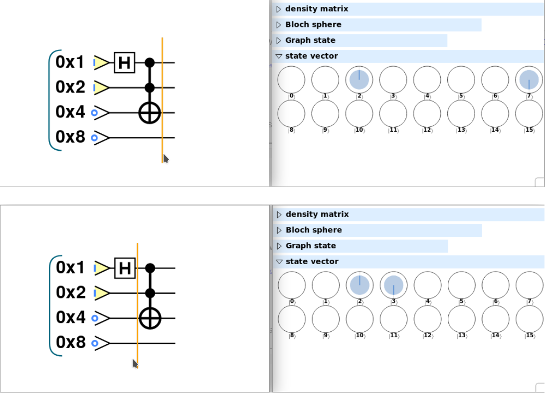
Figure 1-4. Stepping through a QCEngine progam using the circuit and circle-notation visualizers
Now that you have access to a QPU simulator, you’re probably keen to start tinkering. Don’t let us stop you! In Chapter 2 we’ll start to walk through the code for increasingly complex QPU programs.
Native QPU Instructions
QCEngine is one of several tools that allow us to run and inspect QPU code, but what will QPU code actually look like? In conventional CPU programming, software stacks connect many layers of abstractions and tools, from raw hardware controls, to assembly-language instructions, right through to applications written in high-level languages. A similar stack exist for programming a QPU, one that incorporates both quantum and classical elements. Conventional high-level languages are commonly used to control lower level QPU instructions (as we’ve already seen with JavaScript-based QCEngine). In this book we’ll regularly cross between these layers. Describing the programming of a QPU with machine-level operations helps us get to grips with fundamental novel logic of a QPU, whilst seeing how we to manipulate these operations from higher level conventional languages like JavaScript, Python or {cpp} gives us a more pragmatic paradigm for actually writing code.
To whet your appetite, we list some of the fundamental QPU instructions in Table 1-1 below - each of which will be explained in more detail within the chapters ahead. It is worth noting that it is not necessary for a QPU to natively feature all of these instructions; in fact all quantum algorithms can be implemented with a very small set of native gates, in the same way as any classical computation can be made exclusively from NAND gates. However, most QPUs will have an extended set of gate available for use, and this list contains the most common ones.
| Symbol | Name | Usage | Description |
|---|---|---|---|
NOT (also X) |
|
Logical bitwise NOT |
|
CNOT |
|
Controlled NOT: If (c) then NOT(t) |
|
CCNOT (Toffoli) |
|
If (c1 and c2) then NOT(t) |
|
HAD (Hadamard) |
|
Hadamard gate (normally used to create quantum superposition) |
|
PHASE |
|
Relative phase rotation |
|
Z |
|
Relative phase rotation by 180 degrees |
|
S |
|
Relative phase rotation by 90 degrees |
|
T |
|
Relative phase rotation by 45 degrees |
|
CPHASE |
|
Conditional phase rotation |
|
CZ |
|
Conditional phase rotation by 180 degrees |
|
READ |
|
Read and collapse qubits, returning digital data |
|
WRITE |
|
Write digital data to qubits |
|
ROOTNOT |
|
Root-of-NOT operation. |
|
SWAP (EXCHANGE) |
|
Exchange two qubits |
|
CSWAP |
|
Conditonal exchange: if (c) then SWAP(t1 |
With each of these operations, the specific instructions and timing will depend on the processor brand and architecture. However, this is an essential set of basic operations expected to be available on all machines, and these operations form the basis of our QPU programming, just as instructions like MOV and ADD do for CPU programmers.
Simulator Limitations
Although simulators offer us a fantastic opportunity to prototype small QPU programs built from the kind of operations described above, when compared to real QPUs they are hopelessly under-powered. One measure of the power of a QPU is the number of qubits it has available to operate on2 (the quantum equivalent of bits, on which we’ll have much more to say shortly).
At the time of this book’s publication, the world record for the largest QPU that can be simulated with a conventional computer stands at 51 qubits. That’s sort of like simulating a digital computer with 51 total bits of RAM (just over 6 bytes). In practice, the simulations and resources available to most readers of this book will typically be able to handle 26 or so qubits before grinding to a halt.
The examples in this book have been written with these limitations in mind. They make a great starting point, but each qubit added to them will double the memory required to run the simulation, cutting its speed in half.
Hardware Limitations
Conversely, at the time this book is being written, the largest actual QPU hardware available has around 70 physical qubits, whilst the largest QPU available to the public (through the [QISKit](https://qiskit.org/) project) is 16 physical qubits3. By physical, as opposed to logical, we mean that these 70 qubits have no error correction - making them noisy and unstable. Qubits are much more fragile than their conventional counterparts - the slightest interaction with the environment (even something as unassuming as the absorption of a single photon or a collision with a single atom) can derail the computation. What seems an insurmountable hurdle can be overcome by one of the most remarkable results in the field of quantum computing: the threshold theorem. This theorem proves that there exist quantum error correction protocols that allow us to build clean logical qubits from noisy imperfect ones, as long as the imperfections in our hardware are below a certain threshold value.
Dealing with logical qubits allows a programmer can be agnostic about the QPU hardware, and implement any textbook algorithm without having to worry about specific hardware constraints4. In this book, we focus solely on programming with logical qubits, and while the examples we provide are small enough to be run on smaller QPUs (such as the ones available at the time of publication), abstracting away physical hardware details means that the skills and intuitions you develop will remain invaluable as future hardware develops5.
QPU vs. GPU: Some Common Characteristics
The idea of programming an entirely new kind of processor can be intimidating (even if it does already have its own [StackExchange community](https://quantumcomputing.stackexchange.com/). Here’s a list of pertinent facts about what it’s like to program a QPU:
-
It is very rare that a program will run entirely on a QPU. Usually, a program running on the CPU will issue QPU instructions, and later retrieve the results.
-
Some tasks are very well suited to the QPU, and others are not.
-
The QPU runs on a separate clock from the CPU, and usually has its own dedicated hardware interfaces to external devices (optical outputs and such).
-
A typical QPU has its own special RAM which the CPU cannot efficiently access.
-
A simple QPU will be one chip accessed by a laptop, or even perhaps eventually an area within another chip. A more advanced QPU is a large and expensive add-on, and always requires special cooling.
-
Early QPUs, even simple ones, are the size of refrigerators and require special high-amperage power outlets.
-
When a computation is done, a projection of the result is returned to the CPU, and most of the QPU’s internal working data is discarded.
-
QPU debugging can be very tricky, requiring special tools and techniques. Single-stepping a program is sometimes not possible, and often the best approach is to make changes to the program and observe their effect on the output.
-
Optimizations which speed up one QPU may slow down another.
Sounds pretty challenging. But here’s the thing, you can replace QPU with GPU in each and every one of those statements and they’re still entirely valid.
Although QPUs are an almost alien technology of incredible power, when it comes to the problems we might face in learning to program them, a generation of software engineers have seen it all before. It’s true of course that there are some nuances to QPU programming that are genuinely novel (this book wouldn’t be necessary otherwise!), but the uncanny number of similarities should be reassuring. We can do this!
How this book is structured
A tried-and-tested approach for getting hands-on with new programming paradigms is to learn a set of conceptual primitives. For example, anyone learning GPU programming should focus on mastering parallelism and pixel shader concepts, rather than on syntax or hardware specifics.
The heart of our book focuses on building an intuition for a set of quantum primitives – ideas forming a toolbox of building-blocks for problem solving with a QPU. To prepare us for these primitives we first introduce the basic concepts of qubits (the rules of the game if you like). Following outlining the primitives we show how they can be used as building blocks within useful QPU applications
As a consequence, this book is divided into three parts. The reader is encouraged to become familiar with Part I and gain some hands-on experience before proceeding to more advanced parts.
-
Part I: Programming for a QPU - Here we introduce the core concepts required to program a QPU, such as qubit essentials, instructions, superposition logic and even quantum teleportation. Examples are provided, which can be easily run using simulators or a physical QPU.
-
Part II: QPU Primitives - The next part provides detail on some essential algorithms and techniques at a higher level. These include amplitude amplification, the Quantum Fourier Transform, phase estimation, and linear equation solving. These can be considered “library functions” that programmers will call to build applications. Understanding how they work is essential to becoming a skilled QPU programmer. There is an active community of researchers developing new QPU Primitives, therefore we expect this library to grow in the future. An appendix with resources from the research literature is provided for the interested reader who wants to keep up with the state-of-the-art.
-
Part III: QPU Applications - The world of QPU applications is evolving as rapidly as the machines themselves. Here we introduce a few examples of existing applications, as well as some fun speculation on others.
By the end of these three parts of the book we hope to provide the reader with an understanding of what quantum applications can do, what makes them powerful, and how to identify the kinds of problems that they can solve.
Enough introduction. Let’s begin!
1 One of our favorite ways to drive this point home is the following result of a back-of-the-envelope calculation: Suppose conventional transistors could be made atom-sized, and we aimed to build a warehouse-sized conventional computer able to match even a modest quantum computers performance at factoring prime integers. We would need to pack transistors so densely that we would create a gravitational singularity. Gravitational singularities make computing (and existing) very hard.
2 Despite its popularity in the media as a benchmark for quantum computing, counting the number of qubits that a piece of hardware can handle is really an oversimplification, and much subtler considerations are necessary to assess a QPU’s true power.
3 Although it’s possible this figure may even become out of date whilst this book is in press!
4 For example, as well as performing no error correction, current 70 qubit QPUs have restrictions on which qubits can interact with each other - requiring special care if one is working with that particular piece of hardware.
5 Circa 2019, QPUs with logical (error-corrected) qubits do not yet exist. As a consequence discussions of quantum computing sometimes center on applications specifically contrived for less powerful (noisier) QPUs. These are commonly referred to as Noisy Intermediate-Scale Quantum, or NISQ, applications. We will not cover these applications, but rather focus on programming a fully functioning QPU.