Qubits vs. Bits

Conventional bits have one binary parameter that we can play with - we can initialize a bit in either state 0 or state 1. This makes the mathematics of binary logic simple enough to use as-is, but we could visually represent the possible 0/1 values of a bit, using two separate filled/empty circles.

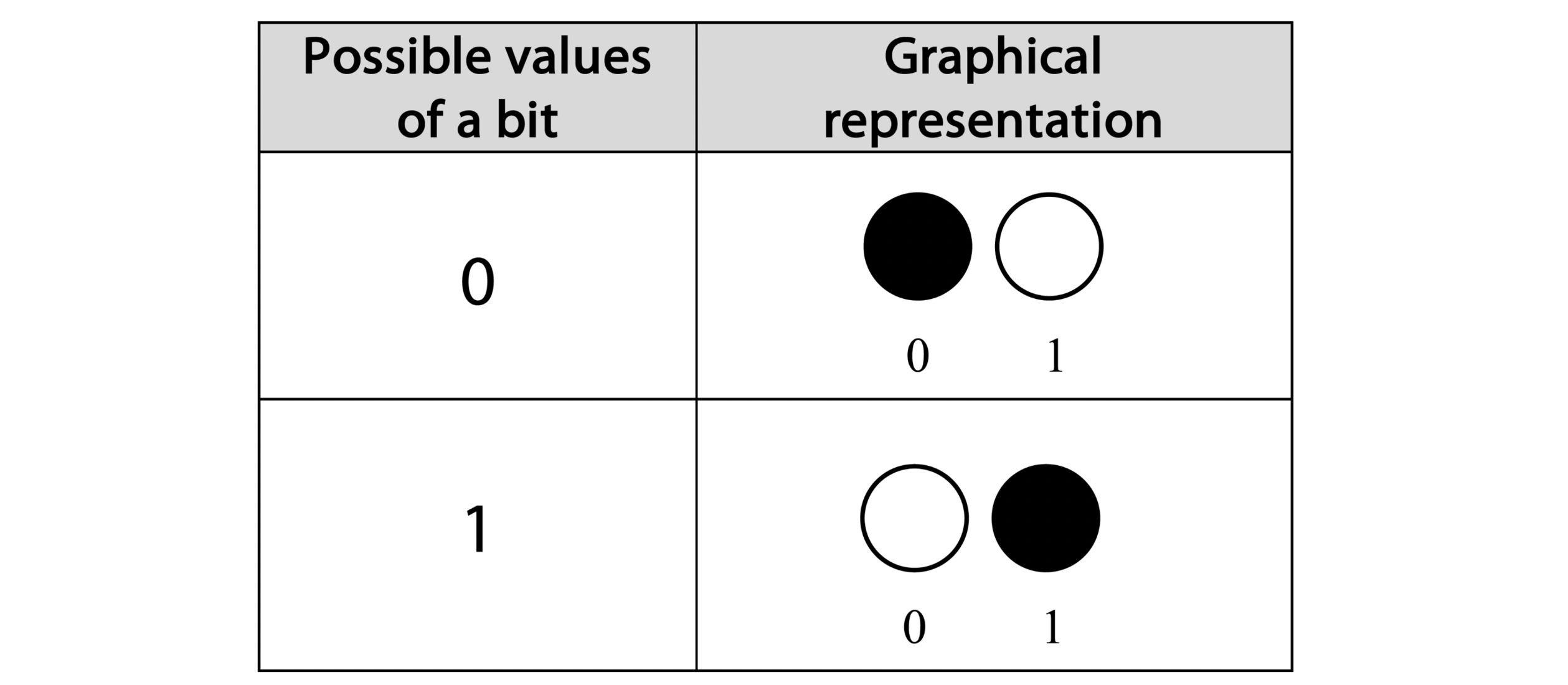
Figure 2-1. Possible values of a conventional bit - a graphical representation

Now onto qubits. In some sense, qubits are very similar to bits – whenever you read the value on a qubit, you’ll always find a value of either 0 or 1. So after the readout of a qubit, we can always describe it as shown in Figure 2-1.

But characterizing qubits before readout isn’t so black and white, and requires a more sophisticated description. Recall from our photon example that we can generate a multitude of different kinds of superpositions by tweaking the parameters of a qubits amplitudes. In fact, the number of possible superpositions that a qubit can exist in before being read forms an infinite continuum. Figure 2-2 lists just some of the variations we could dial up with particular choices of the magnitudes and relative phases of a superposition. Although we’ll always end up reading out 0 or 1 at the end, if we’re clever then it’s the availability of these extra states that will allow us to perform some very powerful computing.

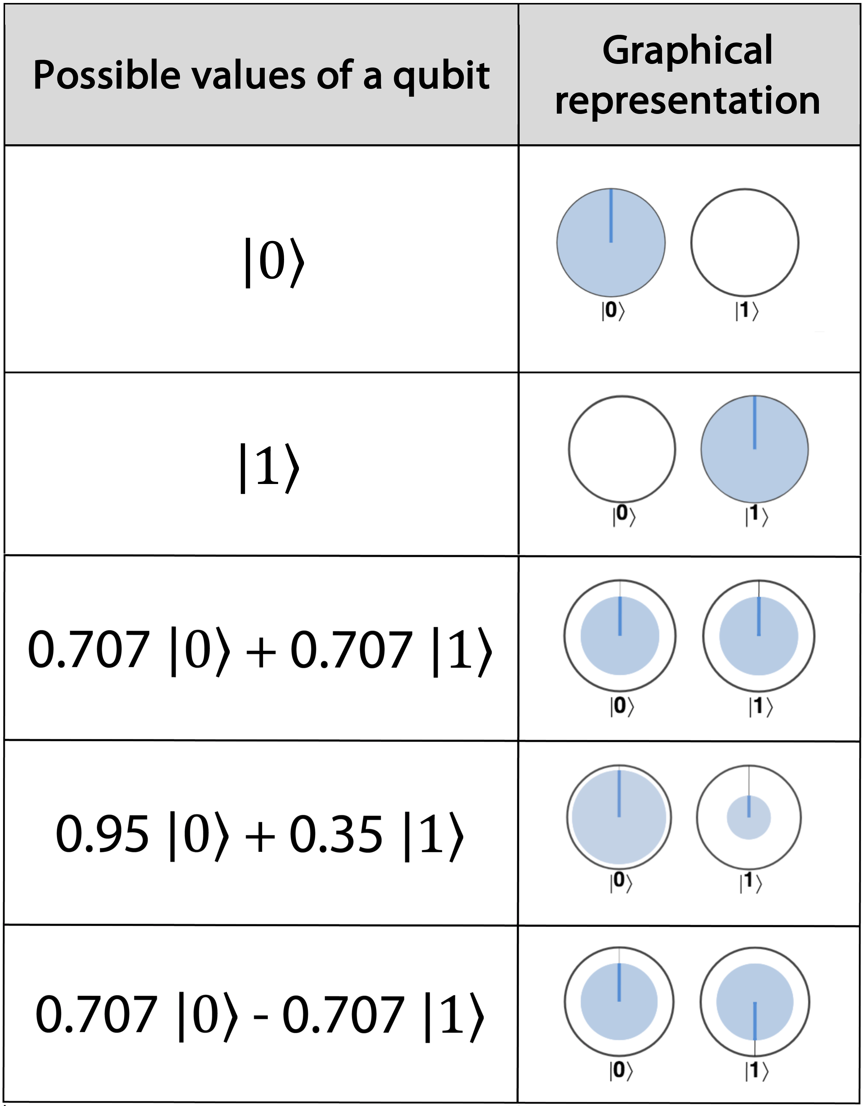
Figure 2-2. Some possible values of a qubit

The first two rows in Figure 2-2 show the quantum equivalents of the states of a conventional bit - with no superposition at all. A qubit prepared in state ∣0〉 is equivalent to a conventional bit being 0 - it will always give a value 0 on read-out - and similarly for ∣1〉. If our qubits were only ever in states ∣0〉 or ∣1〉 (and none of the more exotic combinations illustrated in the other rows) then we’d just have a very expensive conventional bit.

But as soon as we start considering superpositions, the mathematical representations of our qubit shown in the left-hand column of Figure 2-2 begin getting much more involved than the simple binary logic of conventional bits. Fortunately, the right-hand column also presents an equivalent pictorial circle notation. Since our goal is building a fluent and pragmatic intuition for what goes on inside a QPU without needing to entrench ourselves in opaque mathematics, from now on we’ll think of qubits entirely in terms of this circle notation. Let’s see how this notation represents the amplitudes of a qubit in superposition¹.

Introducing Circle Notation

From experimenting with photons we’ve seen that there are two aspects of a qubits general state that we need to keep track of in a QPU - the magnitude of its superposition amplitudes and the relative phase between them. Circle notation displays these parameters as follows:

• The magnitude of the amplitude associated with each value a qubit can assume (∣0〉 or ∣1〉) is related to the fraction of filled-in area shown for each of the ∣0〉 or ∣1〉 circles - or more colloquially, the size of each circle.

• The relative phase between these values amplitudes is indicated by the rotation of the ∣1〉 circle relative to the ∣0〉 circle (a darker line is drawn in the circles to make this rotation apparent).

We’ll be relying on circle notation throughout the book, so it’s worth taking a little more care to see precisely how the sizes and rotations of these circles capture these concepts.

Size of the circles:

The area shaded in each of the circles is directly proportional to the probability of obtaining that circle’s value (0 or 1) if we read out the qubit. The examples in Figure 2-3 show the circle notation for different qubit states and the chance of reading out a 1 in each case.

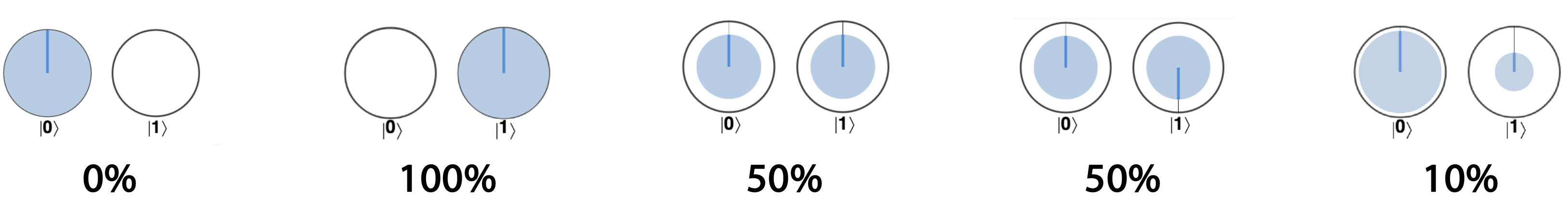
Figure 2-3. Probability of reading the value 1 for different superpositions represented in circle notation

Destructive observation

Reading a qubit destroys information. In all of the above cases, reading the qubit will produce either a 0 or a 1, and when that happens, the qubit will change its state to match the observed value. So even if a qubit was initially in a more sophisticated state, once you readout 1 you’ll always get 1 if you immediately continue to try and read it again.

Notice that as the area shaded in the ∣0〉 circle gets larger, there’s more chance you’ll read out a 0, and of course that means that the chance of getting a 1 outcome decreases (being whatever is left over). In the last example in Figure 2-3, there is a 90% of reading out the qubit as 0, and therefore a corresponding 10% chance of reading out a 1.

It’s easy to forget, although important to remember that in circle notation the size of a circle associated with a given outcome does not represent the full superposition amplitude. The important additional information that we’re missing is the relative phase of our superposition.

Relative rotation of the circles:

Some QPU instructions will also allow us to alter the relative rotations of a qubits ∣0〉 and ∣1〉 circles. This represents the relative phase of the qubit. The relative phase between a qubits state can take any value from to , and a few examples are shown below.

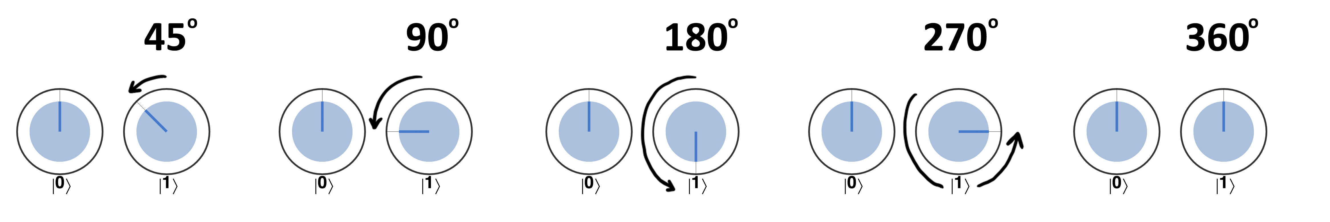
Figure 2-4. Example relative phases in a single qubit

Warning

Our convention for rotating the circles in circle notation within this book is that a positive angle rotates the relevant circle counter-clockwise, as illustrated above.

In all the above example we have only rotated the ∣1〉 circle. Why not the ∣0〉 circle as well? As the name suggests, it’s only the relative phase in a qubit’s superposition that ever makes any difference. And consequently only the relative rotation between our circles² is of interest³. If a QPU operation were to apply a rotation to both circles then we can always consider them both to be rotated such that only the ∣1〉 circle is rotated - making the relative rotation more readily apparent:

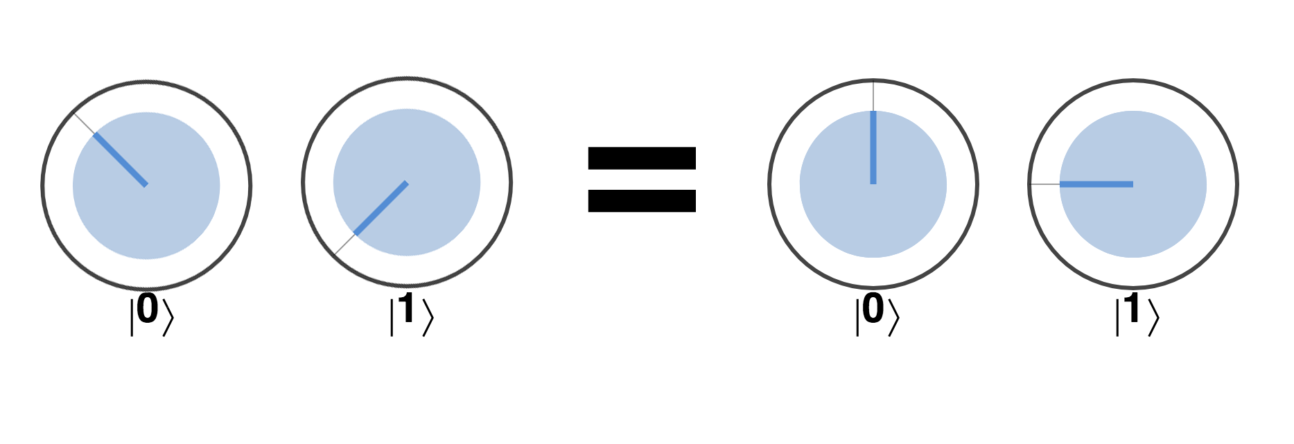
Figure 2-5. Only relative rotations matter in circle notation.

So although sometimes a simulation might show both circles rotated, it’s worth bearing in mind that we can imagine rotating all the circles if it helps us make sense of things.

Note that the relative phase can be varied independently of the magnitude of a superposition (the one exception being that it doesn’t make sense to talk about relative phase if a qubit state is entirely either ∣0〉 or ∣1〉). This independence also works the other way, comparing the third and fourth examples in Figure 2-3 we can see that the relative phase between outcomes for a single qubit has no direct effect on the chances of us reading them out.

The fact that the relative phase of a single qubit has no effect on the magnitudes in a superposition means that it has no influence on observable readout results. Although this may make the relative phase property seem inconsequential, this could not be further from the truth. In quantum computations involving multiple qubits, we can crucially take advantage of this rotation to cleverly and indirectly affect the chances we will eventually read out different values. In fact, by manipulating qubits with carefully chosen operations, well engineered relative phases can provide an astonishing computational advantage. We’ll now introduce some of these operations - in particular those that act only on a single qubit - and we’ll visualize their effects using circle notation.

A Quick Look at a Physical Qubit

Conventional programming guides almost never mention the physical nature of bits and bytes, despite the fascinating truth behind modern silicon fabrication. In fact, the ability to abstract away the physical nature of information is what makes writing complex programs of any kind possible. Similarly, this book will focus on what qubits do rather than what they physically are.

That said, we’d be remiss if we didn’t give some idea of what a qubit actually looks like. Although the transistor has won its way to modern-day ubiquity, a visit to any computer history museum will testify that there are many ways to build digital bits. Similarly, there are many ways to physically create qubits (although at the time of writing we don’t yet know which will become ubiquitous). Any physical object that can be isolated enough from the rest of the universe to display some of the more delicate phenomena of quantum physics can, in principle, be used as a qubit⁴.

One object that readily demonstrates the quantum effects required of a qubit is a single photon. To illustrate this, let’s take a step back and suppose we tried to use the location of a photon to represent a conventional digital bit. In the device shown in Figure 2-6, a switchable mirror (that can be set as either reflective or transparent) allows us to control whether a photon ends in up in one of two paths - corresponding to an encoding of either 0 or 1.

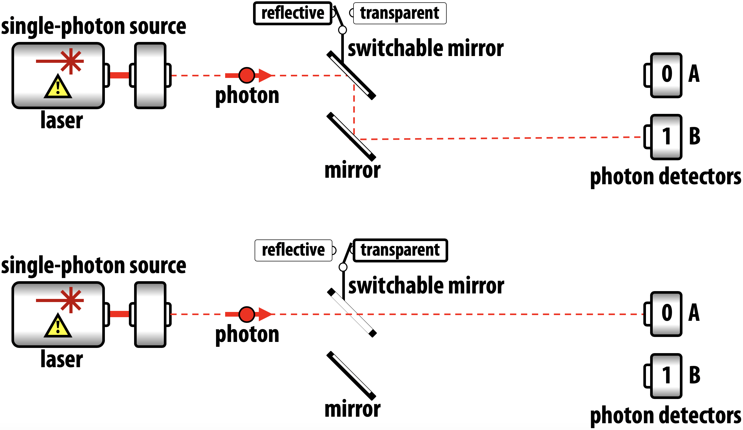
Figure 2-6. Using a photon as a conventional bit

Devices like this actually exist in digital communication technology, but nevertheless a single photon clearly makes a very fiddly bit (for starters, it won’t stay in any one place for very long). To use this setup to demonstrate some qubit properties, suppose we replace the switch we use to set the photon as 0 or 1 with a half-silvered mirror.

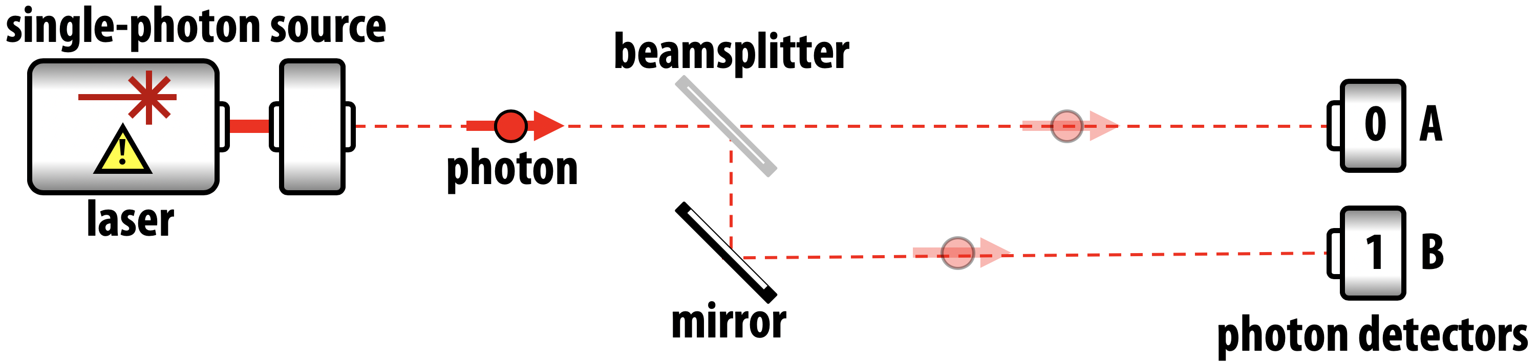
Figure 2-7. A simple implementation of one photonic qubit

A half silvered mirror, as shown in Figure 2-7 (also known as a beamsplitter), is a semi-reflective surface that would, with a 50% chance, either deflect light into the path we associate with 1, or allow it to pass straight through to the path we associate with 0. There are no other options.

When a single, indivisible, photon hits this surface it suffers a sort of identity crisis. In a sense that has no digital equivalent, it ends up existing in a state where it can be influenced by effects in both the 0 path and the 1 path. We say that the photon is in a superposition of traveling in each possible path. In other words, we no longer have a conventional bit, but a qubit that can be in a superposition of values 0 and 1.

It’s very easy to misunderstand the nature of superposition (as many popular quantum computing articles do). It’s not correct to say that the photon is in both the 0 and 1 paths at the same time. There is only one photon, so if we put detectors in each path, as shown in Figure 2-7, only one will go off. When this happens, it will reduce the quantum state of the photon into a digital bit and give a definitive 0 or 1 result. Yet, as we’ll explore shortly, there are computationally useful ways a QPU can interact with a qubit in superposition before we need to read it out through such a detection.

The kind of quantum superposition shown in Figure 2-7 will be central to leveraging the quantum power of a QPU. As such, we’ll need to describe and control quantum superpositions a little more quantitatively. When our photon is in a superposition of paths, we say it has an amplitude associated with each path. There are two important aspects to these amplitudes - two knobs we can twiddle to alter the particular configuration of a qubit’s superposition:

• The magnitude associated with each path of the photon’s superposition is an analog value determining the probability that the photon will be detected in that path. This magnitude is a measure of how much the photon has spread into each path. In Figure 2-7 we could twiddle the magnitudes of the amplitudes associated with each path by altering the reflectivity of the beamsplitter.

• The relative phase between the different paths in the photon’s superposition captures the amount by which the photon is delayed on one path relative to the other. This is also an analog value which can be controlled by the path length difference. Note that we could change the relative phase without affecting the change of the photon being detected in each path.

The magnitude and relative phase are values available for us to exploit when computing, and we can think of them as being encoded in our qubit. But if we’re ever to readout any information from it, the photon must eventually strike a detector. At this point both these analog values vanish - the quantumness of the qubit is gone. Herein lies the crux of quantum computing - finding a way to exploit these ethereal quantities such that some useful remnant remains after the destructive act of readout.

Everything we’ve discussed so far has been specifically related to photons, and we’re in danger of getting a little too attached to the idea of them forming our qubits. There are many physical ways to implement qubits, so we’d like to have a functional model of superposition, magnitude, and relative phase which is not tied to any particular implementation.

This is a programmer’s guide, not a physics textbook, let’s abstract away the physics and see how we can describe and visualize qubits in a manner as detached from photons and quantum physics as binary logic is from semiconductor physics.

The First Few QPU Operations

Like their CPU counterparts, single-qubit QPU instructions take an input and transform it into an output. Only now of course our inputs and outputs are qubits rather than bits. Many QPU instructions have an associated inverse, which can be useful to know about. In this case a QPU operation is said to be reversible, which ultimately means that no information is lost or discarded when it is applied. Some QPU operations however are irreversible and have no inverse (somehow they result in the loss of information). We’ll eventually come to see that whether or not an operation is reversible can have important ramifications for how we make use of it.

Some of these QPU instructions may seem strange and of questionable use - but after only introducing a handful of them we’ll quickly begin putting them to use.

QPU Instruction: NOT

The NOT is the quantum equivalent of a digital NOT operation on a bit. Zero becomes one, and vice versa. However, unlike its conventional cousin the QPU NOT operation also works on a qubit in superposition.

In circle notation this results, very simply, in the swapping of the ∣0〉 and ∣1〉 circles, as in Figure 2-8.

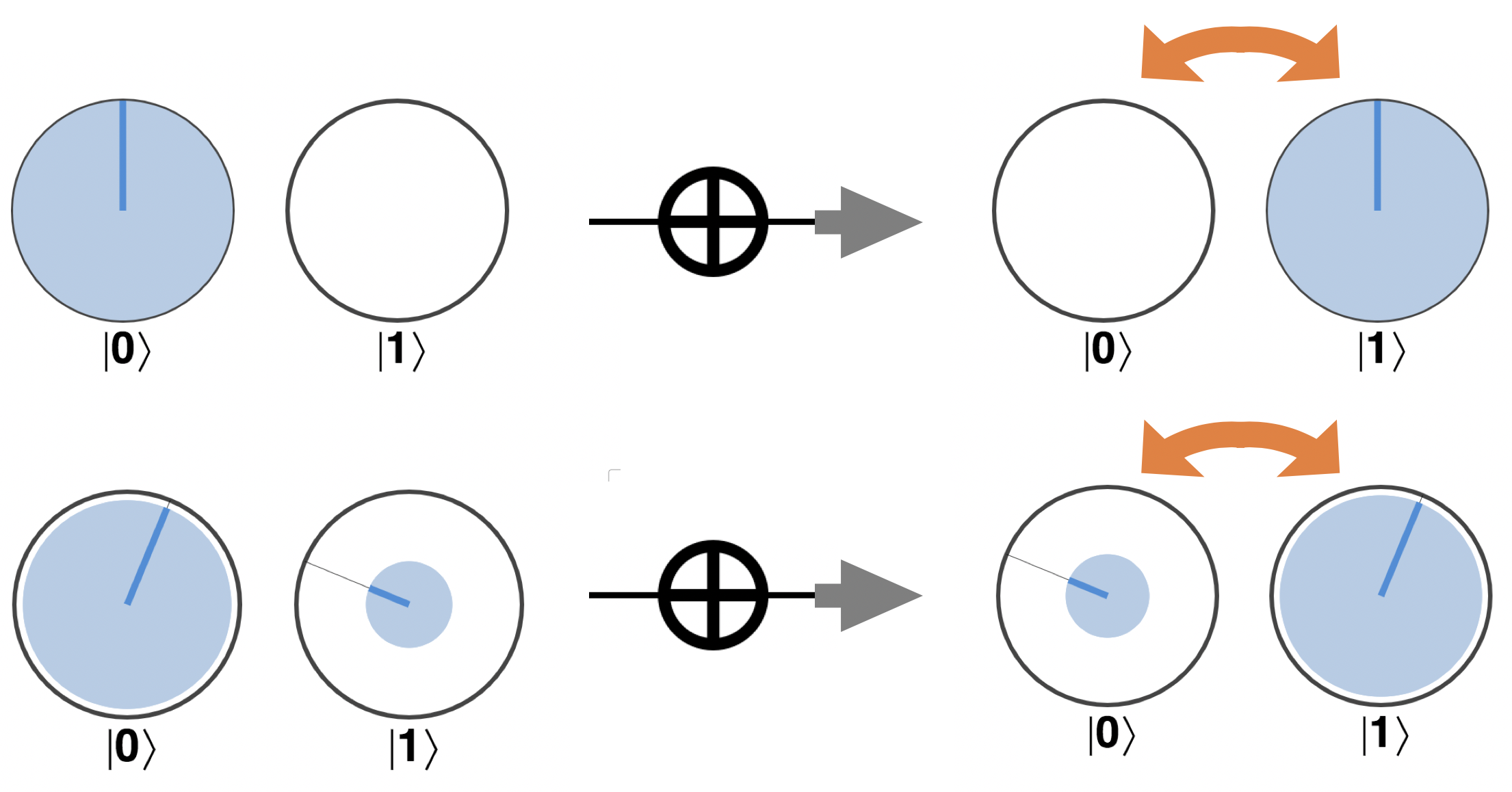
Figure 2-8. The NOT operator in circle notation

Reversibility: Just as in digital logic, the NOT operation is its own inverse; applying it twice returns the qubit to its original value.

QPU Instruction: HAD

The HAD operation (short for Hadamard) is the first QPU instruction we will encounter that cannot be performed on a digital bit.

HAD essentially creates an equal superposition when presented with either a ∣0〉 or ∣1〉 state. This operation is our gateway drug into using the bizarre and delicate parallelism of quantum superposition!

In circle notation, this results in the output qubit having the same amount of area filled-in for both ∣0〉 and ∣1〉, as in Figure 2-9.

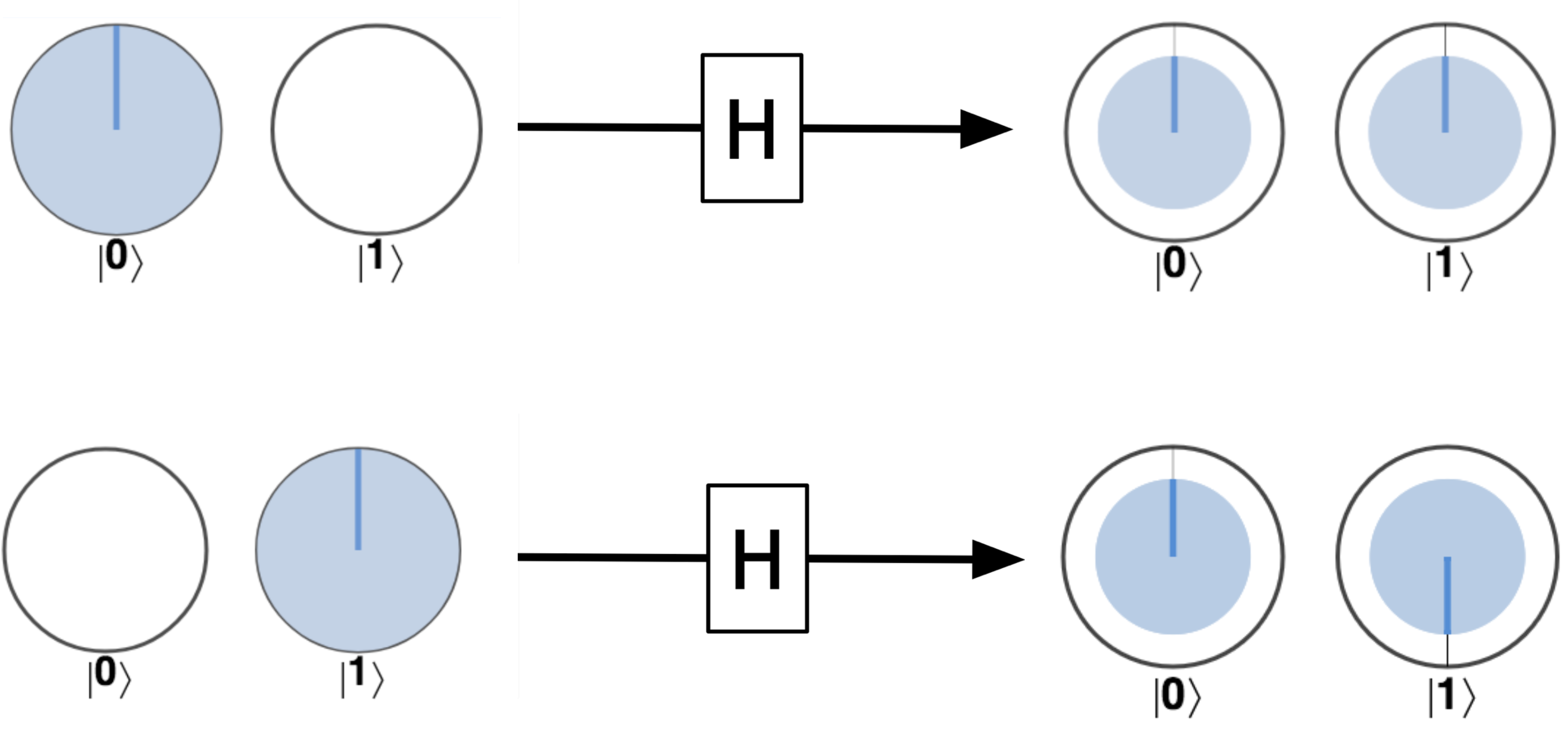
Figure 2-9. Hadamard applied to some basic states

This allows HAD to often be used to produce uniform superpositions of outcomes in a qubit - i.e. a superposition where each outcome is equally likely. Notice also that the action on qubits initially in the states ∣0〉 and ∣1〉 is slightly different - the output of acting HAD on ∣1〉 yields a non-zero rotation (relative phase) of one of the circles, whereas the output from acting it on ∣0〉 doesn’t.

We can also apply HAD to qubits which are already in a superposition. In this case the ∣0〉 value of the output is the sum of the amplitudes from the two input states, and the ∣1〉 value of the output is the difference between these amplitudes - each part being weighted by the original superpositions amplitudes (note that amplitudes are not the same as magnitudes).

We won’t worry about being able to reproduce this example with the (complex) mathematics of superposition amplitudes. In practice we’ll rely on a simulator such as QCEngine to determine the actions of HAD for us in such situations.

Reversibility: Similar to NOT, the HAD operation is its own inverse; applying it twice returns the qubit to its original value.

QPU Instruction: READ and WRITE

The READ operation is the formal expression of the readout process on a qubit that we’ve talked about previously. READ is unique in being the only part of a QPU’s instruction set that potentially returns a random result.

READ will return a value of either 0 or 1 with a probability determined by the magnitude associated with each outcome in a qubits state (ignoring the relative phase). Following a READ operation a qubit is left in a state ∣0〉 if the 0 outcome is obtained and state ∣1〉 if the 1 outcome is obtained. In other words, any superposition is irreversibly destroyed.

In circle notation an outcome occurs with a probability determined by the filled area in each associated circle. We then shift the filled in area between circles to reflect this result - the circle associated with the occurring outcome becomes entirely filled-in, whilst the remaining circle becomes empty. This is illustrated in Figure 2-10 for READ being performed on two different example superpositions.

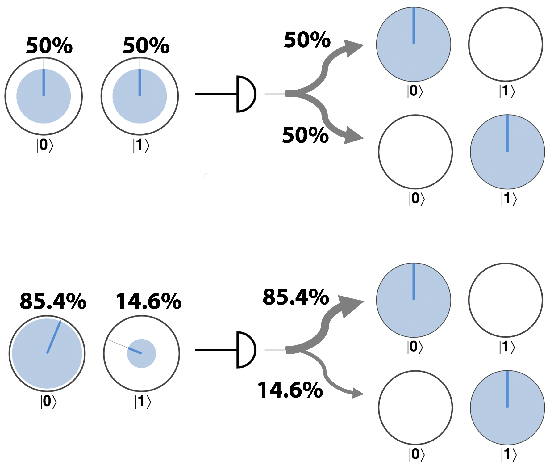
Figure 2-10. The READ operator produces random results

What happened to the phase?

In the second example of Figure 2-10, the READ operation removes all meaningful amplitude and phase information. As a result, we are free to draw the remaining circle at any orientation.

Using READ, we can also construct a simple WRITE operation that allows us to prepare a qubit in a desired state of either ∣0〉 or ∣1〉. This may be performed by combining READ and NOT. First we READ the qubit, and then if the value does not match the value we plan to WRITE, we perform a NOT operation. On some QPU hardware, qubits are initialized to ∣0〉, so simply applying a NOT will set the value to ∣1〉. Note that this WRITE operation does not allow us to prepare a qubit in an arbitrary superposition (with arbitrary magnitude and relative phase), but only in either state ∣0〉 or state ∣1〉⁵

Reversibility: The READ and WRITE ops are not reversible. They cause the quantum state to collapse, and lose information. Once that is done, the analog values of the qubit (both amplitude and phase) are gone forever.

Hands-on: A perfectly random bit

Before moving on to introduce a few more single qubit operations, let’s pause to see how - armed with the HAD, READ and WRITE operations - we can already perform a task that is impossible on any conventional computer. We will generate a truly random bit.

Throughout the history of computation, a vast amount of time and effort has gone into developing PRNG (Pseudo-Random Number Generator) systems, which find usage in applications ranging from cryptography to weather forecasting. PRNGs are pseudo in the sense that if you know the contents of the computer’s memory and the PRNG algorithm, you can predict the next number in the sequence.

According to the known laws of physics the readout behavior of a qubit in superposition is fundamentally and perfectly unpredictable. This allows a QPU to create the worlds greatest random number generator by simply preparing a qubit in state ∣0〉, applying the HAD instruction, and then reading out the qubit. We can illustrate this combination of QPU operations using a quantum circuit diagram, where a line moving left to right illustrates the sequence of different operations that are performed on our (single) qubit.

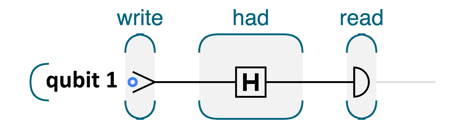
Figure 2-11. Generating a perfectly random bit with a QPU

It might not look like much, but there we have it, our first quantum application - a Quantum Random Number Generator (QRNG)! We can simulate this using the code snippet given below. If you repeatedly run these four lines of code on the QCEngine simulator, you’ll receive a binary random string. Of course CPU-powered simulators like QCEngine are approximating our QRNG with a PRNG, but running the equivalent code on a real QPU will produce a perfectly random binary string.

About these code samples

All of the code samples in this book can be found online at [http://oreilly.machinelevel.com](http://oreilly.machinelevel.com), and may be run either on QPU simulators, or else on actual QPU hardware. Running these samples is an essential part of learning to program a QPU! For more information on running them, see the notes online, or Chapter 1.

Since it might be your first quantum program (congratulations!), let’s break it down just to be sure each step makes sense:

• qc.reset(1) sets up our simulation of the QPU, requesting one qubit. All the programs we write for QCEngine will initialize a set of qubits with a line like this.

• qc.write(0) simply initializes our single qubit in the ∣0〉 state – the equivalent of a conventional bit being set to the value 0.

• qc.had() applies HAD to our qubit, placing it into a superposition of ∣0〉 and ∣1〉, just as in Figure 2-9.

• var result = qc.read() reads out the value of our qubit at the end of the computation, as a random digital bit - assigning the value to the result variable.

Since HAD leaves our qubit with its weighting equally spread over ∣0〉 and ∣1〉, then – pragmatically - after applying HAD to a qubit and reading it out we receive either a 0 or 1 with precisely 50% probability – i.e. we randomly read out a 0 or 1.

It might look like all we’ve really done here is find a very expensive way of flipping a coin, but this underestimates the power of HAD. If you could somehow look inside HAD you would find neither a pseudo nor hardware random generator. Unlike these, HAD is guaranteed unpredictable by the laws of quantum physics. Nobody in the known universe can do any better than a hopeless random guess as to whether a qubit’s value following a HAD will be read to be 0 or 1 – even if they know exactly the instructions we are using to generate our random numbers.

So, a QPU’s instruction set contains a fundamental single instruction that can produce truly random bits for us - straight out of the box!

In fact, although we’ll properly introduce dealing with multiple qubits in the next chapter, we can easily see, how by running our program for a single random qubit in parallel eight times, we can produce a random qubyte. Example 2-2 shows what this looks like.

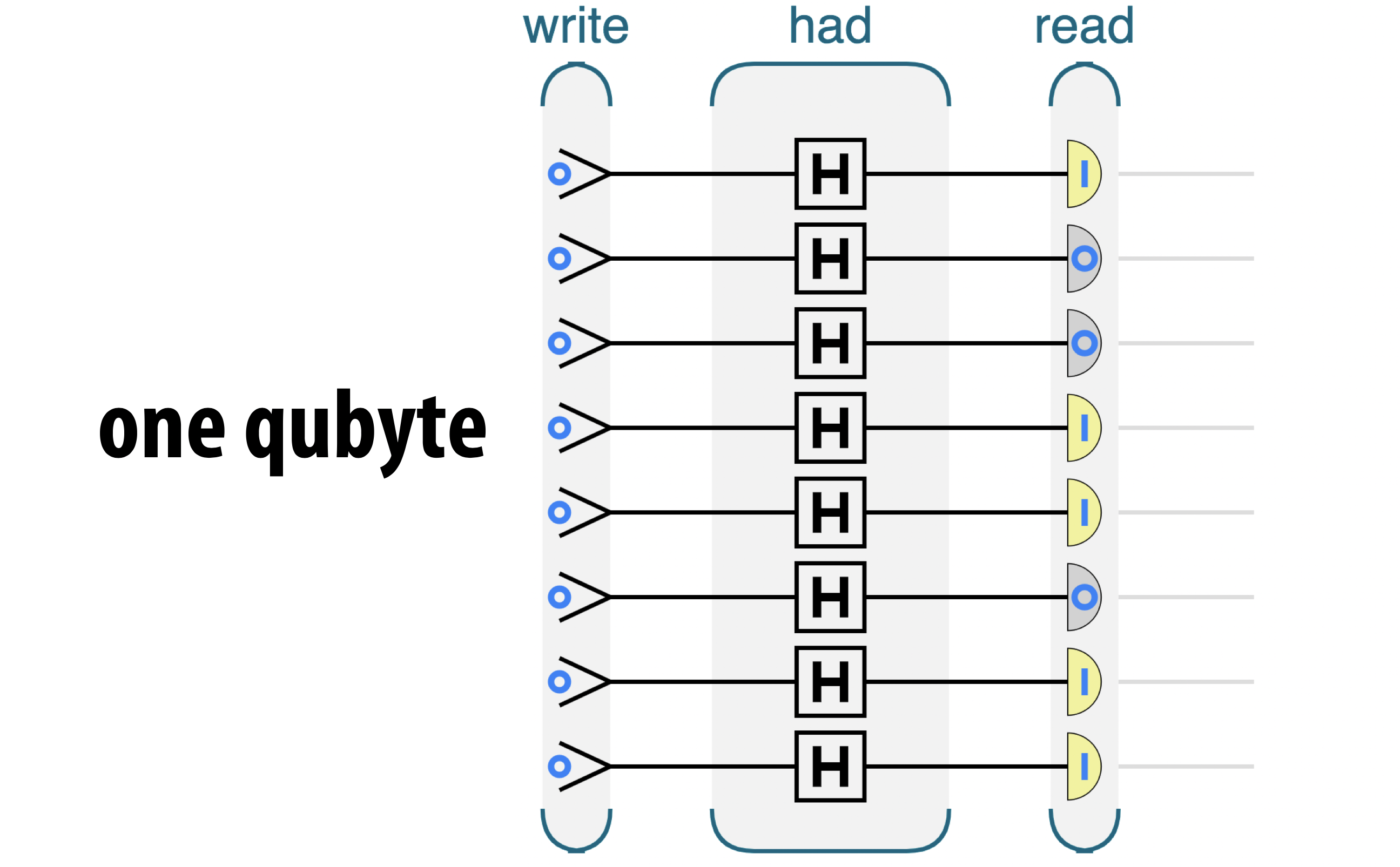
Figure 2-12. One random byte

This code for creating a random qubyte is of course almost identical to Example 2-1, just expanded to eight qubits:

Note that above we make use of the fact that in QCEngine operations like WRITE and HAD default to being applied to all qubits that we have initialized, unless we explicitly pass specific qubits for them to act on.

Eight separate qubits

Although Example 2-2 uses multiple qubits, there are no actual multi-qubit operations that take more than on of the qubits as input. The same program could be run on a simple 1-qubit processor, by generating random bits one at a time.

QPU Instruction: PHASE()

The PHASE() operator, like HAD, has no classical-bit equivalent. This instruction allows us to directly manipulate the relative phase of a qubit - changing it by some specified angle. Consequently, as well as a qubit to operate on, the PHASE() operation also takes an additional (conventional) parameter as an input - the angle to rotate by. For example, PHASE(45), denotes a PHASE operation that performs a 45 degree rotation.

In circle notation the effect of PHASE() is to simply rotate the circle associated with ∣1〉 by the angle we specify. This is shown in Figure 2-13 for the case of PHASE(45).

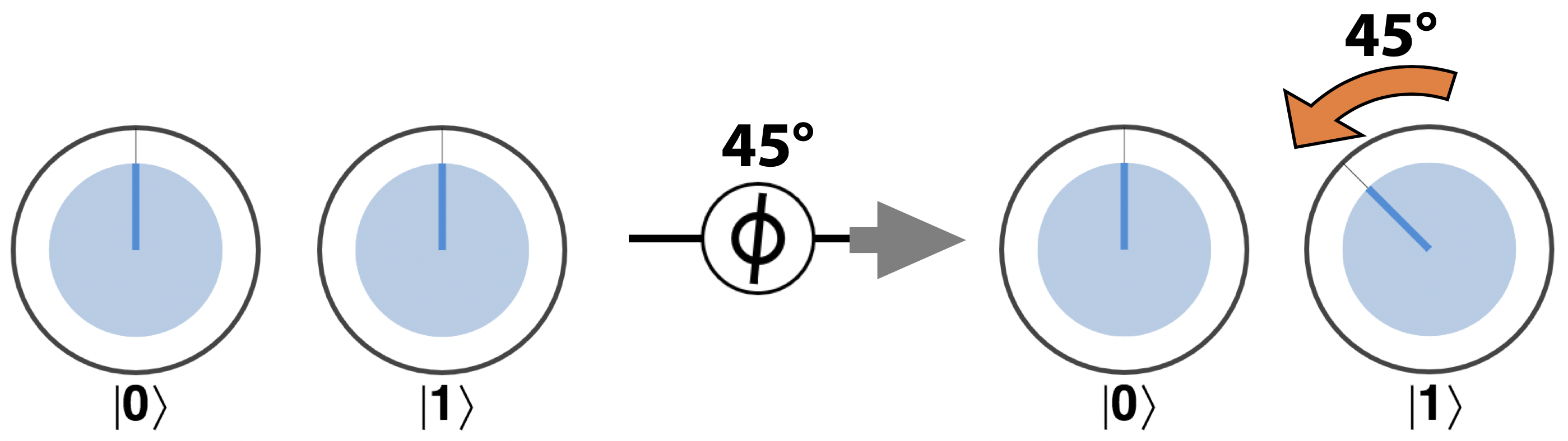
Figure 2-13. Operation of a PHASE gate

Note that the PHASE operation only rotates the circle associated with the ∣1〉 state, and has no effect on a qubit in the ∣0〉 state.

Reversibility: PHASE operations are reversible, although they are not generally their own inverse. The PHASE operation may be reversed by applying a PHASE with the negative of the original angle. In circle notation, this corresponds to undoing the rotation, by rotating in the opposite direction.

Using HAD and PHASE, we can produce some single-qubit quantum states which are so commonly used that they’ve been named: ∣+〉, ∣-〉, ∣+Y〉, and ∣-Y〉, as seen in Figure 2-14. If you’re feeling like flexing your QPU muscles, see whether you can determine how to produce these states using HAD and PHASE operations (each superposition shown has an equal magnitude in each of the ∣0〉 and ∣1〉 states).

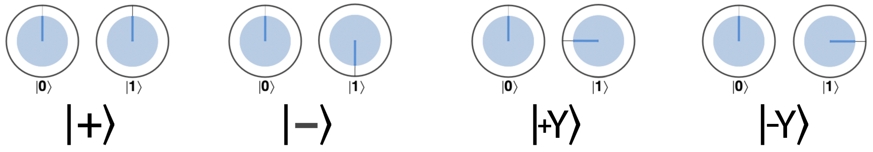
Figure 2-14. Four very commonly used single-qubit states

These four states will be used in Example 2-4, and in fact although they can be produced using HAD and PHASE, we can also understand them as being the result of so-called single-qubit rotation operations. These rotations do not correspond to rotations in the circle notation, but to rotations in a different visualization of qubits that is used in the academic literature (if you want to learn about it, you can check chapter ).

One final note on PHASE() - At a glance, the ability of PHASE to rotate a term may seem less powerful than HAD’s ability to create superposition and allow a sort of parallel computation. This is far from the truth, as a computation that only involves HAD gates and not PHASE can be efficiently simulated on a classical computer. It is only when those gates are combined (together with the two qubit gates that we will see in Chapter 3) that the full computational power of the quantum computer can be attained.

QPU Instructions: ROTX() and ROTY() rotation operations

We’ve seen that PHASE rotates the relative phase of a qubit - and that in circle notation this corresponds to rotating the circle associated with the ∣1〉 value. There are two other common operations related to PHASE called ROTX() and ROTY(), which also perform kinds of rotations on our qubit.

Here’s what the application of ROTX(45) and ROTY(45) looks like on the ∣0〉 and ∣1〉 states in our circle notation:

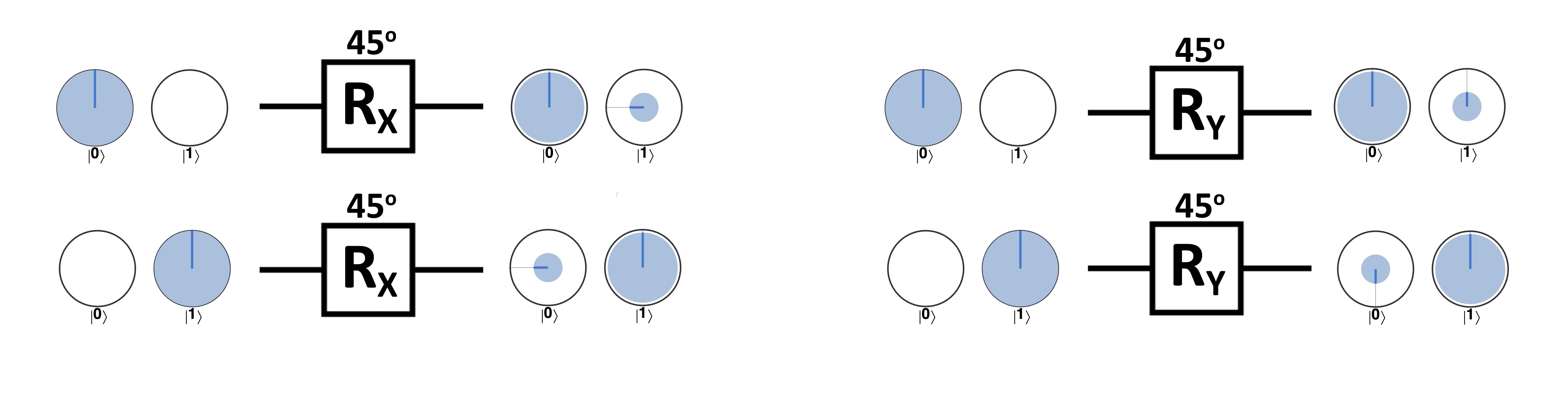
Figure 2-15. ROTX and ROTY actions on 0 and 1 input states.

In our circle notation these operations don’t look like very intuitive rotations, at least not as obviously as PHASE did. However, their rotation names stem from their action in another common visual representation of a single qubits state, known as the Bloch sphere. In the Bloch sphere representation, a qubit is visualized by a point somewhere on the surface of three-dimensional sphere. We use circle notation instead of the Bloch sphere visualization in this book as the Bloch sphere doesn’t scale up well when dealing with multiple qubits. But to satisfy any etymological curiosity, if we were to represent a qubit on the Bloch sphere then ROTY and ROTX operations would correspond to rotating the point representing the qubit about the sphere’s Y and X axes respectively⁶]:] - although this meaning is lost in our circle notation, since we use two 2D circles rather than a three dimensional sphere. In fact, the PHASE operation actually corresponds to a rotation about the Z axis when visualizing qubits in the Bloch sphere, and so you may also here it referred to as ROTZ.

2D rotations on a 4D object

If you do want to try visualizing ROTX and ROTY as rotations similar to PHASE (also called ROTZ), consider this: In circle notation, each of our 2D circles for ∣0〉 and ∣1〉 has two axes. PHASE performs a 2D rotation using the two axes in the ∣1〉 circle, while ROTX and ROTY do the same thing, but using one axis from each circle.

You may have noticed that the states in Figure 2-15 are precisely those we highlighted in Figure 2-14. In fact the states ∣+〉, ∣-〉, ∣+Y〉, and ∣-Y〉 are precisely what we obtain by rotating our the states ∣0〉 and ∣1〉 with ROTX and ROTY through 90 degrees.

The missing operation

Looking at all the single qubit operations we have presented so far, it might look like the gateset for quantum computation is simply an advanced package of the gateset available to conventional computer. This is not true, as there is one operation that not only quantum computers cannot do better, they cannot do at all: COPY. A strange consequence from the nature of the physical laws that govern quantum systems, the no-cloning theorem states that it is impossible to replicate an unknown quantum state. Of course through repeated preparation, we can make many copies of a known state, but there is no way of copying a state without first determining what that state is.

This is a bit of an inconvenience at first, but as we will learn in the following chapters, the possibilities available with the new gates make up for loosing COPY.

Combining QPU operations

We now have NOT, HAD, PHASE, READ and WRITE at our disposal. It’s worth mentioning that, just like digital logic, combining these operations can allow us to find alternative ways to realize operations, and even allow us to create entirely new ones. For example, suppose your QPU has the HAD and PHASE instructions, but the NOT is missing. A PHASE(180) gate can be combined with two HADs to produce the exact equivalent of a NOT gate, as shown in Figure 2-16

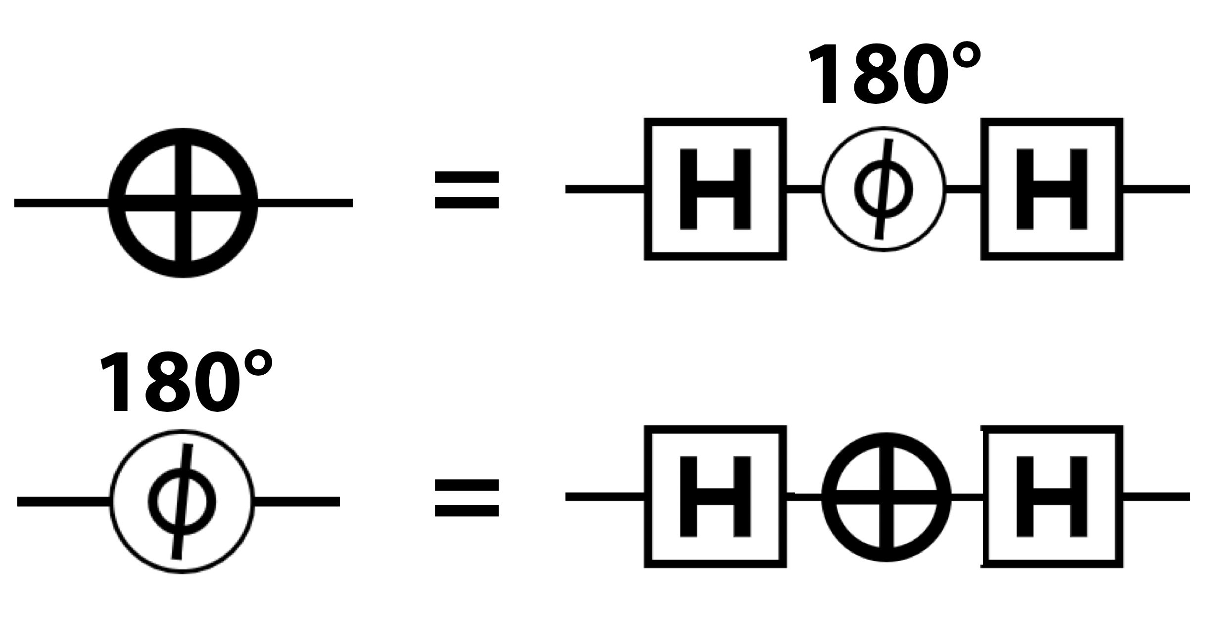
Figure 2-16. Building equivalent gates

See whether you can program the above combination of operations in QCEngine and setup through the resulting circle notation to see how HAD, followed by a PHASE(180) and another HAD results in the same action as a simple NOT.

QPU Combo Instruction: ROOT-of-NOT

Combining gates also lets us produce interesting new gates which do not exist at all in the world of digital logic. The ROOT-of-NOT gate (RNOT) is a great example. It’s quite literally the square-root of the NOT gate, in the sense that, when applied twice, it performs a single NOT operation:

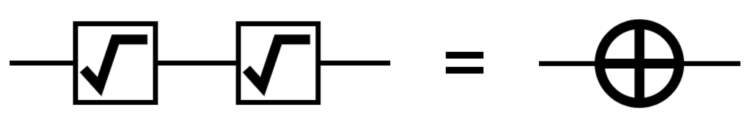
Figure 2-17. An impossible operation for classical bits

There’s more than one way to construct this gate, but here’s one simple implementation:

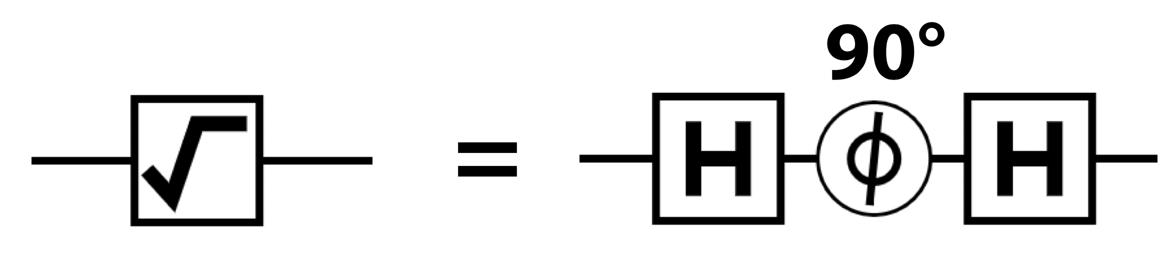
Figure 2-18. Recipe for root-of-not

We can check that applying this set of gates twice does indeed yield the same result as a NOT by running it in our simulator:

Note

qc.codelabel("op1") is a QCEngine function that allowing us to tag blocks of code with the label specified inside (op1 in this case). The labels show up in QCEngines quantum circuit visualizer and can be useful for making sense of large quantum circuits. Any code following a qc.codelabel("op1") call will be assigned the label we pass to the function. To end the block of code that is tagged, sinply use qc.codelabel().

In circle notation we can visualize each step involved in implementing an RNOT operation (a PHASE(90) between two HADs):

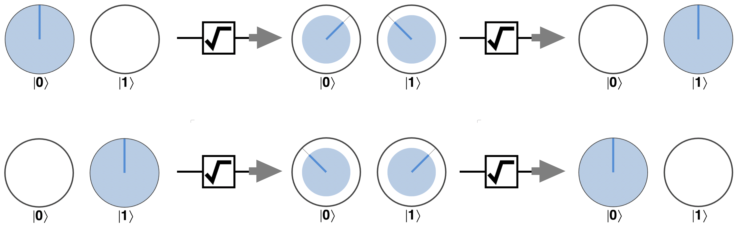
Figure 2-19. Operation of the ROOT-of-NOT gate

Following the evolution of our qubit in circle notation helps us see how RNOT is able to get us halfway to a NOT operation. Recall from Figure 2-16 that if we HAD a qubit, then rotate its relative phase by 180 degrees, another HAD would result in a NOT operation. RNOT performs half of this rotation (a PHASE(90)), so that two applications will result in the HAD-PHASE(180)-HAD sequence that is equivalent to a NOT. It might be a bit mind-bending at first, but see if you can piece together how the RNOT gate cleverly performs this feat when applied twice (it might help to remember that HAD is it’s own inverse, so a sequence of two HADs does nothing at all).

Reversibility: While RNOT operations are never their own inverse, the inverse of the operation in Figure 2-18 may be constructed by using the negative phase value, as shown in Figure 2-20.

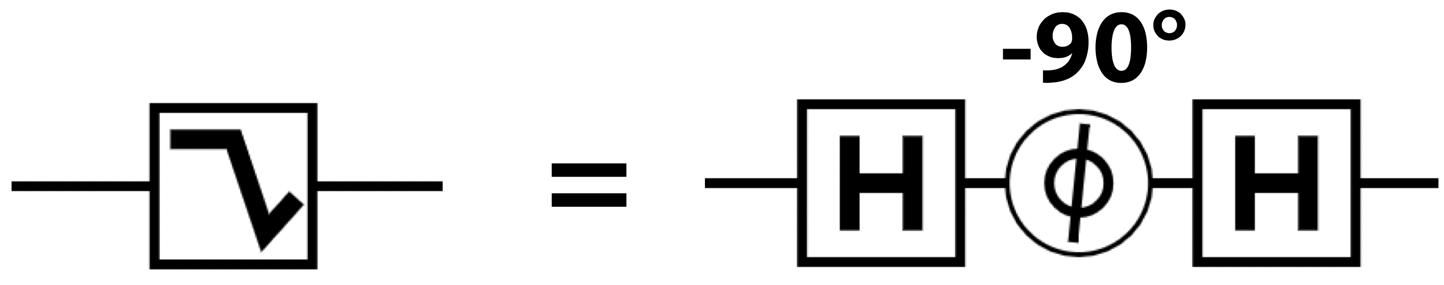
Figure 2-20. Inverse of root-of-not

Although it might seem like an esoteric curiosity, the RNOT gate teaches us the important lesson that by carefully placing information in the relative phase of a qubit we can perform entirely new kinds of computation.

Hands-on: Quantum Spy Hunter

To give a more practical demonstration of the power in manipulating the relative phases of qubits, let’s finish this chapter with a more complex program. One that uses some of the simple single-qubit QPU operations that we’ve learned so far to detect a spy. This technique is a simplified version of QKD (quantum key distribution) which is the core of so-called quantum encryption. The main feature of quantum (as opposed to conventional) key distribution, is that we have the ability to unambiguously detect when a key has been compromised.

We suppose that two QPU programmers, Alice and Bob, are sending data to each other via a communication channel capable of transmitting qubits (turns out that a fiber-optic link will do the job). Once in a while, they send the specially constructed “spy hunter” qubit shown in this example, which they use to test whether their communication channel has been compromised.

Any spy who tries to read one of these qubits has a 25% chance of getting caught. So even if Alice and Bob only use 50 of them in the whole transfer, the spy’s chances of getting away are far less than one in a million.

Alice and Bob can then detect whether their key has been compromised by exchanging some digital (non-quantum) information, which does not need to be private or encrypted. After exchanging their message they test a few of their qubits by reading them out and checking that they agree with the digital in a certain expected way. If any disagree, then they know someone was listening in.

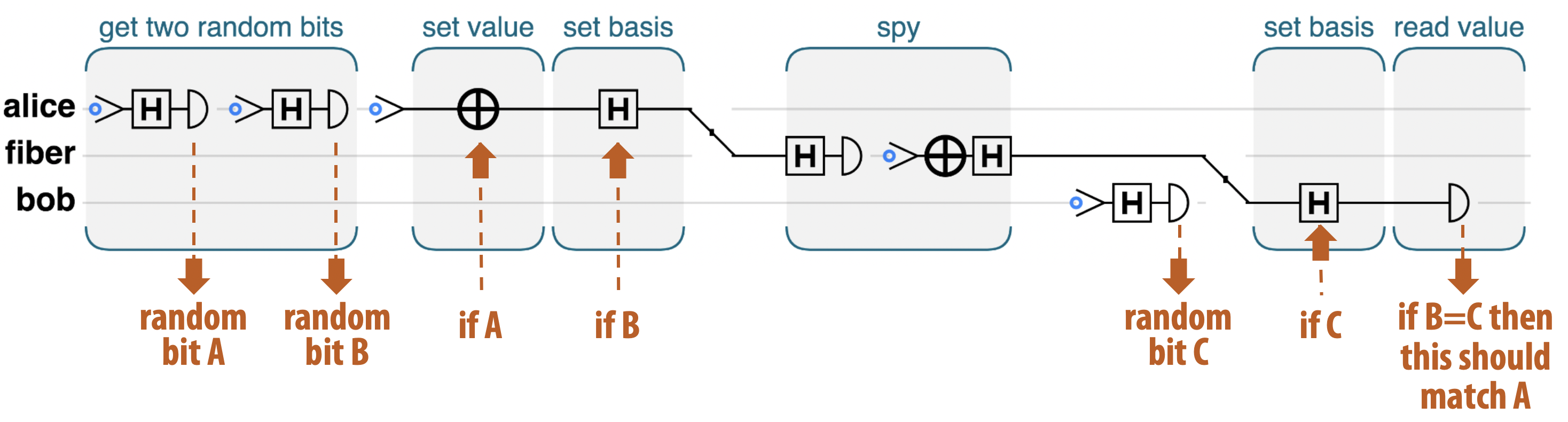
Figure 2-21. Quantum spy hunter

Here’s the code. We strongly recommend trying it out on your own, by pasting the code into the QCEngine workbench link, and tweaking and testing like you would with any other code snippet.

In Example 2-4, Alice and Bob each have access to a simple QPU containing a single qubit, and can send their qubits along a fiber-optic link. There might be a spy listening to that link; in the sample code you can control whether or not a spy is present by toggling the spy_is_present variable.

The fact that quantum cryptography can be performed with such relatively small QPU’s is one of the reasons why it has begun to see commercial application far before more powerful general purpose QPU’s are available.

Let’s walk through the code one step at a time to see how Alice and Bob’s simple QPU’s allow them to perform this feat. We’ll use the comments from the code-snippet as markers:

// Generate two random bits

Alice uses her one-qubit QPU as a simple QRNG, exactly as we did in Example 2-2, to generate two secret random bits known only to her, which we label as basis and value.

// Prepare Alice’s qubit

Using her two random bits, Alice prepares the “spy hunter” qubit. She sets it to value, and then uses basis to decide whether to apply a HAD. In effect, she is preparing her qubit randomly into one of the states ∣0〉, ∣1〉, ∣+〉, ∣-〉, and not (yet) telling anyone which of the states it is. If she does decide to apply a HAD then if Bob wants to extract whether she intended a 0 or 1, he will have to apply the inverse of HAD (another HAD) before performing a READ.

// Send the qubit!

Alice sends her qubit into the fiber connection, on its way to Bob. For clarity in this example, we are using another qubit to represent the fiber.

// Activate the spy

If this were non-quantum digital data, the spy would simply make a copy of the bit. Mission accomplished! With qubits, that’s not possible. Recall that there is no copy operation, so the only thing the spy can do is READ the qubit Alice sent, and then carefully send one just like it to Bob to avoid detection. Remember that reading a qubit destroys information, we are only left with the classical bit of the readout. The spy doesn’t know whether or not Alice performed a HAD. As a result he won’t know whether to apply a second (inverting) HAD before performing his READ. If he simply performs a READ he won’t know whether he’s receiving a random value from a qubit in superposition or a value actually encoded by Alice. Not only does this mean he won’t be able to reliably extract Alice’s bit, but he also won’t know what the right state is to send on to Bob to avoid detection.

// Receive the qubit

Like Alice, Bob randomly generates a basis bit, and uses that to decide whether to apply a HAD before applying a READ to Alice’s qubit, resulting in his value bit. This means that sometimes Bob will (by chance) correctly decode a binary value from Alice and other times he won’t.

// If the basis matches and the value does not, there’s a spy!

Now that the qubit has been received, Alice and Bob can openly compare in which cases their choices of applying HAD’s or not correctly matched up. If they randomly happened to both apply (or not apply) a HAD (this will be about half the time) then their value bits should match - i.e. Bob correctly decoded Alice’s message. If, in these correctly decoded messages their values don’t agree, then they can conclude that the spy must have READ their message and sent on an incorrect replacement qubit to Bob - messing up his decoding.

Conclusion

In this chapter we have introduced a logical model for a single qubit, as well as a variety of QPU instructions used to manipulate it. The quantum random property of the READ operation was used to construct a random number generator, and control over the phase of a qubit was used to detect a spy.

The ability to combine single-qubit operations into new operations is important to understand, and can be critical when using a QPU program on hardware or simulators with differing instruction sets. Similar construction methods will be used to build new operations in the chapters ahead.

The circle notation used to visualize the state of a qubit is also used extensively in the chapters ahead, where it is expanded to display the state of multi-qubit systems. In the next chapter, we will explore the logical behavior of these multi-qubit systems, and also introduce new QPU operations used to work with them.