Set up the execution environment

The first thing a Flink application needs to do is set up its execution environment. The execution environment determines whether the program is running on a local machine or on a cluster. In the DataStream API, the execution environment of an application is represented by the StreamExecutionEnvironment. In our example, we retrieve the execution environment by calling the getExecutionEnvironment(). This method returns a local or remote environment, depending on the context in which the method is invoked. If the method is invoked from a submission client with a connection to a remote cluster, a remote execution environment is returned. Otherwise, it returns a local environment.

It is also possible to explicitly create local or remote execution environments as follows:

// create a local stream execution environment
val localEnv: StreamExecutionEnvironment.createLocalEnvironment()

// create a remote stream execution environment
val remoteEnv = StreamExecutionEnvironment.createRemoteEnvironment(
  "host",                // hostname of JobManager
  1234,                  // port of JobManager process
  "path/to/jarFile.jar)  // JAR file to ship to the JobManager

The JAR file that is shipped to the JobManager must contain all resources that are required to execute the streaming application. 

Next, we use env.setStreamTimeCharacteristic(TimeCharacteristic.EventTime) to instruct our program to interpret time semantics using event time. The execution environment allows for more configuration options, such as setting the program parallelism and enabling fault tolerance.

Read an input stream

Once the execution environment has been configured, it is time to do some actual work and start processing streams. The StreamExecutionEnvironment provides methods to create a stream source that ingests data streams into the application. Data streams can be ingested from sources such as message queues, files, or also be generated on the fly.

In our example, we use

val sensorData: DataStream[SensorReading] = 
  env.addSource(new SensorSource)

to connect to the source of the sensor measurements and create an initial DataStream of type SensorReading. Flink supports many data types which we describe in the next section. Here, we use a Scala case class as the data type that we defined before. A SensorReading contains the sensor id, a timestamp denoting when the measurement was taken, and the measured temperature. The following two methods configure the input data source to be executed with a parallelism of 4 by calling setParallelism(4) and assign timestamps and watermarks, which are required for event time using assignTimestampsAndWatermarks(new SensorTimeAssigner). The implementation details of SensorTimeAssigner should not concern us for the moment.

Apply transformations

Once we have a DataStream, we can apply a transformation on it. There are different types of transformations. Some transformations can produce a new DataStream, possibly of a different type, while other transformations do not modify the records of the DataStream but reorganize it by partitioning or grouping. The logic of an application is defined by chaining transformations.

In our example, we first apply a map() transformation, which converts the temperature of each sensor reading to celsius. Then, we use the keyBy() transformation to partition the sensor readings by their sensor id. Subsequently, we define a timeWindow() transformation, which groups the sensor readings of each sensor id partition into tumbling windows of 5 seconds. Window transformations are described in detail in the next chapter. Finally, we apply a user-defined function (UDF) that computes the average temperature on each window. We discuss more about defining UDFs in the DataStream API later in this chapter.

Output the result

Streaming applications usually emit their result to some external system, such as Apache Kafka, a file system, or a database. Flink provides a well maintained collection of stream sinks that can be used to write data to different systems. It is also possible to implement own streaming sinks. There are also applications that do not emit results but keep them internally to serve them via Flink’s queryable state feature.

In our example, the result is a DataStream[SensorReading] with the average measured temperature over 5 seconds of each sensor. The result stream is written to the standard output by calling print(). 

Please note that the choice of a streaming sink affects the end-to-end consistency of an application, i.e., whether the result of the application is provided with at-least once or exactly-once semantics. The end-to-end consistency of the application depends on the integration of the chosen stream sinks with Flink’s checkpointing algorithm. We will discuss this topic in more detail in Chapter 7.

Execute

When the application has been completely defined, it can be executed by calling StreamExecutionEnvironment.execute(). Flink programs are lazy executed. That is, that all methods to create stream sources and transformation have not resulted in any data processing so far. Instead, the execution environment constructs an execution plan which starts from all stream sources created from the environment and includes all transformations which are transitively applied to these sources.

Only when execute() is called, the system triggers the execution of the constructed plan. Depending on the type of execution environment, an application is locally executed or sent to a remote JobManager for execution.

Supported Data Types

Flink supports the many common data types that you are used to working with already. The most widely used types can be grouped into the following categories:

• Primitives
• Java and Scala tuples
• Scala case classes
• POJOs, including classes generated by Apache Avro
• Flink Value types
• Some special types

Types that are not especially handled are treated as generic types and serialized using the Kryo serialization framework. 

Let us look into each type category by example.

Primitives

All Java and Scala primitive types, such as Int  (or Integer for Java), String, and Double, are supported as DataStream types. Here is an example that processes a stream of Long values and increments each element:

val numbers: DataStream[Long] = env.fromElements(1L, 2L, 3L, 4L)
numbers.map( n => n + 1)

Java and Scala tuples

Tuples are composite data types that consist of a fixed number of typed fields.

The Scala DataStream API uses regular Scala tuples. Below is an example that filters a DataStream of tuples with two fields. We will discuss the semantics of the filter transformation in the next section: 

// DataStream of Tuple2[String, Integer] for Person(name, age)
val persons: DataStream[(String, Integer)] = env.fromElements(
  ("Adam", 17), 
  ("Sarah", 23))

// filter for persons of age > 18
persons.filter(p => p._2 > 18)

Flink provides efficient implementations of Java tuples. Flink’s Java tuples can have up to 25 fields and each length is implemented as a separate class, i.e., Tuple1, Tuple2, up to, Tuple25. The tuple classes are strongly typed.

We can rewrite the filtering example in the Java DataStream API as follows:

// DataStream of Tuple2<String, Integer> for Person(name, age)
DataStream<Tuple2<String, Integer>> persons = env.fromElements(
  Tuple2.of("Adam", 17), 
  Tuple2.of("Sarah", 23));

// filter for persons of age > 18
persons.filter(new FilterFunction<Tuple2<String, Integer>() {
   @Override
   public boolean filter(Tuple2<String, Integer> p) throws Exception {
       return p.f1 > 18;
   }
})

Tuple fields can be accessed by the name of their public fields f0, f1, f2, etc. as above or by position using the Object getField(int pos) method, where indexes start at 0:

Tuple2<String, Integer> personTuple = Tuple2.of("Alex", "42");
Integer age = personTuple.getField(1); // age = 42

In contrast to their Scala counterparts, Flink’s Java tuples are mutable, such that the values of fields can be reassigned. Hence, functions can reuse Java tuples in order to reduce the pressure on the garbage collector.

personTuple.f1 = 42;         // set the 2nd field to 42
personTuple.setField(43, 1); // set the 2nd field to 43

Scala case classes

Flink supports Scala case classes; classes that can be decomposed by pattern matching. Case class fields are accessed by name. In the following example, we define a case class Person with two fields, name and age. Similar as for the tuples, we filter the DataStream by age.

case class Person(name: String, age: Int)

val persons: DataStream[Person] = env.fromElements(
  Person("Adam", 17), 
  Person("Sarah", 23))

// filter for persons with age > 18
persons.filter(p => p.age > 18)

POJOs

Flink analyzes each type that does not fall into any category and checks if it can be identified and handled as a POJO type. Flink accepts a class as POJO if it satisfies the following conditions:

• It is a public class
• It has a public constructor without any arguments, a.k.a. default constructor.
• All fields are public or accessible through getters and setters. The getter and setter functions must follow the default naming scheme, i.e., Y getX() and setX(Y x) for a field x of type Y.
• All fields have types that are supported by Flink.

For example, the following Java class will be identified as a POJO by Flink:

public class Person {
  // both fields are public
  public String name;
  public int age;

  // default constructor is present
  public Person() {}

  public Person(String name, int age) {
      this.name = name;
      this.age = age;
  }
}

DataStream<Person> persons = env.fromElements(
   new Person("Alex", 42),
   new Person("Wendy", 23)); 

Avro generated classes are automatically identified by Flink and handled as POJOs.

Flink Value types

Value types implement the org.apache.flink.types.Value interface. The interface consists of two methods read() and write() to implement serialization and deserialization logic. For example, the methods can be leveraged to encode common values more efficiently than general-purpose serializers. 

Flink comes with a few built-in Value types, such as IntValue, DoubleValue, and StringValue, that provide mutable alternatives for Java’s and Scala’s immutable primitive types.

Special types

Flink supports several special-purpose types, such as Scala’s Either, Option, and Try types, and Flink’s Java version of the Either type. Similarly to Scala’s Either, it represents a value of one of two possible types, Left or Right. In addition, Flink supports primitive and object Array types, Java Enum types and Hadoop Writable types.

Type Hints

In many cases, Flink is able to automatically infer types and choose the appropriate serializers and comparators. Sometimes, though, this is not a straightforward task. For example, Java erases generic type information. Flink tries to reconstruct as much type information as possible via reflection, using function signatures and subclass information. Type inference is as well possible when the return type of a function depends on its input type. If a function uses generic type variables in the return type that cannot be inferred from the input type, you can give Flink hints about your types using the returns() method.

You can provide type hints with a class, as in the following example:

DataStream<MyType> result = input
   .map(new MyMapFunction<Long, MyType>())
   .returns(MyType.class);

If the function uses generic type variables in the return type that cannot be inferred from the input type, you need to provide a TypeHint instead:

DataStream<Integer> result = input
   .flatMap(new MyFlatMapFunction<String, Integer>())
   .returns(new TypeHint<Integer>(){});

class MyFlatMapFunction<T, O> implements FlatMapFunction<T, O> {

   public void flatMap(T value, Collector<O> out) { ... }
}

TypeInformation

The central class in Flink’s type system is TypeInformation. It provides the system with the necessary information it needs to generate serialiazers and comparators. For instance, when you join or group by some key, this is the class that allows Flink to perform the semantic check of whether the fields used as keys are valid. 

You might in fact use Flink for a while without ever needing to worry about this class, as it usually does all type handling for you automatically. However, when you start writing more advanced applications, you might want to define your own types and tell Flink how to handle them efficiently. In such cases, it is helpful to be familiar with some of the class details.

TypeInformation maps fields from the types to fields in a flat schema. Basic types are mapped to single fields and tuples and case classes are mapped to as many fields as the class has. The flat schema must be valid for all type instances, thus variable length types like collections and arrays are not assigned to individual fields, but they are considered to be one field as a whole.

The following example defines a TypeInformation and a TypeSerializer for a 2-tuple:

// get the execution config
val config = inputStream.executionConfig

...

// create the type information
val tupleInfo: TypeInformation[(String, Double)] =
    createTypeInformation[(String, Double)

// create a serializer
val tupleSerializer = typeInfo.createSerializer(config)

import org.apache.flink.streaming.api.scala._

Basic transformations

Basic transformations process individual events. We explain their semantics and show code examples.

filter [DataStream -> DataStream]

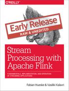
The filter transformation drops or forwards events of a stream by evaluating a boolean condition on each input event. A return value of true preserves the input event and forwards it to the output, false results in dropping the event. A filter transformation is specified by calling the DataStream.filter() method. Figure 5.2 shows a filter operation that only preserves white squares.

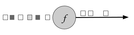
Figure 5-1. A filter operation that only retains white values.

The boolean condition is implemented as an UDF either using the FilterFunction interface or a lambda function. The FilterFunction interface is typed on the type of the input stream and defines the filter() method that is called with an input event and returns a boolean. 

// T: the type of elements
FilterFunction[T]
    > filter(T): Boolean

The following example shows a filter that drops all sensor measurements with temperature below 25 degrees:

val readings: DataStream[SensorReadings] = ...
val filteredSensors = readings
    .filter( r =>  r.temperature >= 25 )

map [DataStream -> DataStream]

The map transformation is specified by calling the DataStream.map() method. It passes each incoming event to a user-defined mapper that returns exactly one output event, possibly of a different type. Figure 5.1 shows a map transformation that converts every square into a circle.

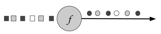
Figure 5-2. A map operation that transforms every square into a circle of the same color.

The mapper is typed to the types of the input and output events and can be specified using the MapFunction interface. It defines the map() method that transforms an input event into exactly one output event.

// T: the type of input elements
// O: the type of output elements
MapFunction[T, O]
    > map(T): O

Below is a simple mapper that projects the first field (id) of each ATLAS-CURSOR-SensorReading in the input stream:

val readings: DataStream[SensorReading] = ...
val sensorIds: DataStream[String] = readings.map(new MyMapFunction)

class MyMapFunction extends ProjectionMap[SensorReading, String] {
  override def map(r: SensorReading): String = r.id
}

When using the Scala API or Java 8, the mapper can also be expressed as a lambda function.

val readings: DataStream[SensorReading] = ...
val sensorIds: DataStream[String] = readings.map(r => r.id)

flatMap [DataStream -> DataStream]

FlatMap is similar to map, but it can produce zero, one, or more output events for each incoming event. In fact, flatMap is a generalization of filter and map and it can be used to implement both those operations. Figure 5.3 shows a flatMap operation that differentiates its output based on the color of the incoming event. If the input is a white square, it outputs the event unmodified. Black squares are duplicated, and gray squares are filtered out.

Figure 5-3. A flatMap operation that outputs white squares, duplicates black squares, and drops gray squares.

The flatMap transformation applies a UDF on each incoming event. The corresponding FlatMapFunction defines the flatMap() method, which may return none, one, or more events as result by passing them to the Collector object.

// T: the type of input elements
// O: the type of output elements
FlatMapFunction[T, O]
    > flatMap(T, Collector[O]): Unit

The example below shows a flatMap transformation that transforms the stream of sensor String ids. Our simple event source for sensor readings produces sensor ids of the form “sensor_N”, where N is an integer. The flatMap function below separates each id into its prefix, “sensor_” and the sensor number and emits them both:

val sensorIds: DataStream[String] = ...
val splitIds: DataStream[String] = sensorIds
  .flatMap(id => id.split("_"))

Note that each word will be emitted as an individual record, that is flatMap flattens the output collection.

KeyedStream transformations

A common requirement of many applications is to process groups of events together that share a certain property. The DataStream API features the abstraction of a KeyedStream, which is a DataStream that has been logically partitioned into disjoint substreams of events that share the same key.

Stateful transformations that are applied on a KeyedStream read from and write to state in the context of the currently processed event’s key. This means that all events with the same key can access the same state and thereby be processed together. Please note that stateful transformations and keyed aggregates have to be used with care. If the key domain is continuously growing, for example because the key is a unique transaction ID, then the application might eventually suffer from memory problems. Please refer to Chapter 8 which discusses stateful functions in detail. 

A KeyedStream can be processed using the map, flatMap, and filter transformations that you saw before. In the following you will see how to use a keyBy transformation to convert a DataStream into a KeyedStream and keyed transformations such as rolling aggregations and reduce. 

keyBy [DataStream -> KeyedStream]

The keyBy transformation converts a DataStream into a KeyedStream using a specified key. Based on the key, it assigns events to partitions. Events with different keys can be assigned to the same partition, but it is guaranteed that elements with the same key will always be in the same partition. Hence, a partition consists of possibly multiple logical substreams, each having a unique key. 

Considering the color of the input event as the key, Figure 5.4 below assigns white and gray events to one partition and black events to the other:

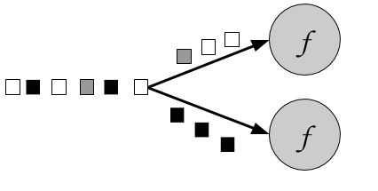
Figure 5-4. A keyBy operation that partitions together events based on their color.

The keyBy() method receives an argument that specifies the key (or keys) to group by and returns a KeyedStream. There are different ways to specify keys. We look into them in the section “Defining Keys" later in the chapter. The following example groups the sensor readings stream by id:

val readings: DataStream[SensorReading] = ...
val keyed: KeyedStream[SensorReading, String] = readings
  .keyBy(_.id)

Rolling aggregations [KeyedStream -> DataStream]

Rolling aggregation transformations are applied on a KeyedStream and produce a stream of aggregates, such as sum, minimum, and maximum. A rolling aggregate operator keeps an aggregated value for every observed key. For each incoming event, the operator updates the corresponding aggregate value and emits an event with the updated value. A rolling aggregation does not require an user-defined function but receives an argument that specifies on which field the aggregate is computed. The DataStream API provides the following rolling aggregation methods:

• sum():  a rolling sum of the input stream on the specified field
• min(): a rolling minimum of the input stream on the specified field
• max(): a rolling maximum of the input stream on the specified field
• minBy(): a rolling minimum of the input stream that returns the event with the lowest value observed so far
• maxBy(): a rolling maximum of the input stream that returns the event with the highest value observed so far

It is not possible to combine multiple rolling aggregation methods, i.e., only a single rolling aggregate can be computed at a time. 

Consider the following example:

val inputStream: DataStream[(Int, Int, Int)] = env.fromElements(
  (1, 2, 2), (2, 3, 1), (2, 2, 4), (1, 5, 3))

val resultStream: DataStream[(Int, Int, Int)] = inputStream
  .keyBy(0) // key on first field of the tuple
  .sum(1)   // sum the second field of the tuple

resultStream.print()

In the example the tuple input stream is keyed by the first field and the rolling sum is computed on the second field. The output of the example is (1,2,2) followed by (1,7,2) for the key “1” and (2,3,1) followed by (2,5,1) for the key “2”. The first field is the common key, the second field is the sum and the third field is not defined.

reduce [KeyedStream -> DataStream]

The reduce transformation is a generalization of the rolling aggregations. It applies a user-defined function on a KeyedStream, which combines each incoming event with the current reduced value. A reduce transformation does not change the type of the stream, i.e., the type of the output stream is the same as the type of the input stream.

The UDF can be specified with a class that implements the ReduceFunction interface. ReduceFunction defines the reduce() method which takes two input events and returns an event of the same type. 

// T: the element type
ReduceFunction[T]
    > reduce(T, T): T

In the example below, the stream is keyed by language and the result is a continuously updated list of words per language:

val inputStream = env.fromElements(

("en", List("tea")), ("fr", List("vin")), ("fr", List("fromage")),   

("en", List("cake")))

inputStream.keyBy(0).reduce((x, y) => (x._1, x._2 ::: y._2)).print()

Multi-stream transformations

Many applications ingest multiple streams that need to be jointly processed or have the requirement to split a stream in order to apply different logic to different substreams. In the following, we discuss the DataStream API transformations that process multiple input streams or emit multiple output streams.

union [DataStream* -> DataStream]

Union merges one or more input streams into one output stream. Figure 5.5 shows a union operation that merges black and white events into a single output stream.

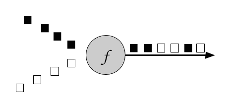
Figure 5-5. A union operation that merges two input streams into one.

The DataStream.union() method receives one or more DataStreams of the same type as input and produces a new DataStream of the same type. Subsequent transformations process the elements of all input streams.

val parisStream: DataStream[SensorReading] = ...
val tokyoStream: DataStream[SensorReading] = ...
val rioStream: DataStream[SensorReading] = ...
val allCities = parisStream.union(tokyoStream, rioStream)

connect, coMap, and coFlatMap [ConnectedStreams -> DataStream]

Sometimes it is necessary to associate two input streams that are not of the same type. A very common requirement is to join events of two streams. Consider an application that monitors a forest area and outputs an alert whenever there is a high risk of fire. The application receives the stream of temperature sensor readings you have seen previously and an additional stream of smoke level measurements. When the temperature is over a given threshold and the smoke level is high, the application emits a fire alert.

The DataStream API provides the connect transformation to support such use-cases. The DataStream.connect() method receives a DataStream and returns a ConnectedStreams object, which represents the two connected streams. 

// first stream
val first: DataStream[Int] = ...
// second stream
val second: DataStream[String] = ...

// connect streams
val connected: ConnectedStreams[Int, String] = first.connect(second)

The ConnectedStreams provides map() and flatMap() methods that expect a CoMapFunction and CoFlatMapFunction as argument respectively.

Both functions are typed on the types of the first and second input stream and on the type of the output stream and define two methods, one for each input. map1() and flatMap1() are called to process an event of the first input and map2() and flatMap2() are invoked to process an event of the second input.

// IN1: the type of the first input stream
// IN2: the type of the second input stream
// OUT: the type of the output elements
CoMapFunction[IN1, IN2, OUT]
    > map1(IN1): OUT
    > map2(IN2): OUT

// IN1: the type of the first input stream
// IN2: the type of the second input stream
// OUT: the type of the output elements
CoFlatMapFunction[IN1, IN2, OUT]
    > flatMap1(IN1, Collector[OUT]): Unit
    > flatMap2(IN2, Collector[OUT]): Unit

Please note that it is not possible to control the order in which the methods of CoMapFunction and CoFlatMapFunction are called. Instead a method is  called as soon as an event has arrived via the corresponding input.

Joint processing of two streams usually requires that events of both streams are deterministically routed based on some condition to be processed by the same parallel instance of an operator. By default, connect() does not establish a relationship between the events of both streams such that the events of both streams are randomly assigned to operator instances. This behavior yields non-deterministic results and is usually not desired. In order to achieve deterministic transformations on ConnectedStreams , connect() can be combined with keyBy() or broadcast() as follows:

// first stream
val first: DataStream[(Int, Long)] = ...
// second stream
val second: DataStream[(Int, String)] = ...

// connect streams with keyBy
val keyedConnect: ConnectedStreams[(Int, Long), (Int, String)] = first
  .connect(second)
  .keyBy(0, 0) // key both input streams on first attribute

// connect streams with broadcast
val keyedConnect: ConnectedStreams[(Int, Long), (Int, String)] = first
  .connect(second.broadcast()) // broadcast second input stream

Using keyBy() with connect() will route all events from both streams with the same key to the same operator instance. An operator that is applied on a connected and keyed stream has access to keyed state ¹. All events of a stream, which is broadcasted before it is connected with another stream, are replicated and sent to all parallel operator instances. Hence, all elements of both input streams can be jointly processed. In fact, the combinations of connect() with keyBy() and broadcast() resemble the two most common shipping strategies for distributed joins: repartition-repartition and broadcast-forward. 

The following example code shows a possible simplifiecd implementation of the fire alert scenario:

// ingest sensor stream
val tempReadings: DataStream[SensorReading] = env
  .addSource(new SensorSource)
  .assignTimestampsAndWatermarks(new SensorTimeAssigner)

// ingest smoke level stream
val smokeReadings: DataStream[SmokeLevel] = env
  .addSource(new SmokeLevelSource)
  .setParallelism(1)

// group sensor readings by their id
val keyed: KeyedStream[SensorReading, String] = tempReadings
  .keyBy(_.id)

// connect the two streams and raise an alert
// if the temperature and smoke levels are high
val alerts = keyed
  .connect(smokeReadings.broadcast)
  .flatMap(new RaiseAlertFlatMap)

alerts.print()

class RaiseAlertFlatMap extends CoFlatMapFunction[SensorReading, SmokeLevel, Alert] {

  var smokeLevel = SmokeLevel.Low

  override def flatMap1(in1: SensorReading, collector: Collector[Alert]): Unit = {
    // high chance of fire => true
    if (smokeLevel.equals(SmokeLevel.High) && in1.temperature > 100) {
      collector.collect(Alert("Risk of fire!", in1.timestamp))
    }
  }

  override def flatMap2(in2: SmokeLevel, collector: Collector[Alert]): Unit = {
    smokeLevel = in2
  }
}

Please note that the state (smokeLevel) in this example is not checkpointed and would be lost in case of a failure.

split [DataStream -> SplitStream] and select [SplitStream -> DataStream]

Split is the inverse transformation to the union transformation. It divides an input stream into two or more output streams. Each incoming event, can be routed to none, one, or more output streams. Hence, split can also be used to filter or replicate events. Figure 5.6 shows an operator all white events into a separate stream than the rest.

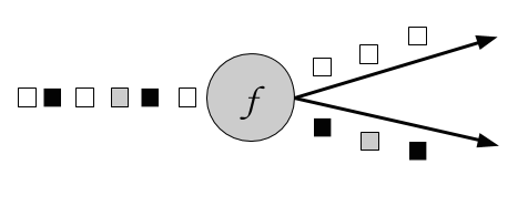
Figure 5-6. A split operation that splits the input stream into a stream of white events and a stream of others.

The DataStream.split() method receives an OutputSelector which defines how stream elements are assigned to named outputs. The OutputSelector defines the select() method which is called for each input event and returns a java.lang.Iterable[String]. The strings represent the names of the outputs to which the element is routed.

// IN: the type of the split elements
OutputSelector[IN]
    > select(IN): Iterable[String]

The DataStream.split() method returns a SplitStream, which provides a select() method to select one or more streams from the SplitStream by specifying listing the output names.

The following example splits a stream of numbers into a stream of large numbers and a stream small numbers.

val inputStream: DataStream[(Int, String)] = ...

val splitted: SplitStream[(Int, String)] = inputStream
  .split(t => if (t._1 > 1000) Seq("large") else Seq("small"))

val large: DataStream[(Int, String)] = splitted.select("large")
val small: DataStream[(Int, String)] = splitted.select("small")
val all: DataStream[(Int, String)] = splitted.select("small", "large") 

Partitioning transformations

Partitioning transformations correspond to the data exchange strategies that we introduced in Chapter 2. These operations define how events are assigned to tasks. When building applications with the DataStream API the system automatically chooses data partitioning strategies and routes data to the correct destination depending on the operation semantics and the configured parallelism. Sometimes, it is necessary or desirable to control the partitioning strategies in the application level or define custom partitioners. For instance, if we know that the load of the parallel partitions of a DataStream is skewed, we might want to rebalance the data to evenly distribute the computation load of subsequent operators. Alternatively, the application logic might require that all tasks of an operation receive the same data or that events are distributed following a custom strategy. In this section, we present DataStream methods that enable users to control partitioning strategies or define their own.

Note that keyBy() is different from the partitioning transformations discussed in this section. All transformation in this section produce a DataStream whereas  keyBy() results in a KeyedStream, on which transformation with access to keyed state can be applied.

Random

The random data exchange strategy is implemented by the shuffle() method of the DataStream API. The method distributes data events randomly according to a uniform distribution to the parallel tasks of the following operator.

Round-Robin

The rebalance() method partitions the input stream so that events are evenly distributed to successor tasks in a round-robin fashion.

Rescale

The rescale() method also distributes events in a round-robin fashion, but only to a subset of successor tasks. In essence, the rescale partitioning strategy offers a way to perform a lightweight load rebalance when the dataflow graph contains fan-out patterns. The fundamental difference between rebalance() and rescale() lies in the way task connections are formed. While rebalance() will create communication channels between all sending tasks to all receiving tasks, rescale() will only create channels from each task to some of the tasks of the downstream operator. The connection pattern difference between rebalance and rescale is shown in the following figures:

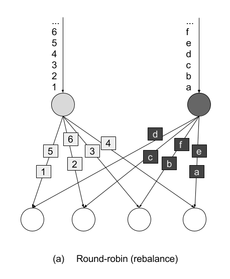
Figure 5-7. Rebalance transformation

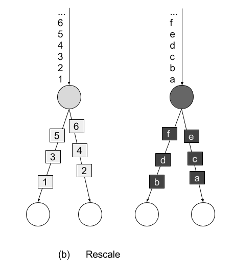
Figure 5-8. Rescale transformation

Broadcast

Global

The global() method sends all events of the input data stream to the first parallel task of the downstream operator. This partitioning strategy must be used with care, as routing all events to the same task might impact the application performance.

Custom

When none of the predefined partitioning strategies is suitable, you can define your own custom partitioning strategy using the partitionCustom() method. The method receives a Partitioner object that implements the partitioning logic and the field or key position on which the stream is to be partitioned. The following example partitions a stream of integers so that all negative numbers are sent to the first task and all other numbers are sent to a random task:

val numbers: DataStream[(Int)] = ...
numbers.partitionCustom(myPartitioner, 0)

object myPartitioner extends Partitioner[Int] {
  val r = scala.util.Random

  override def partition(key: Int, numPartitions: Int): Int = {
    if (key < 0) 0 else r.nextInt(numPartitions)
  }
}