First Edition
Fundamentals, Implementation, and Operation of Streaming Applications
Copyright © 2019 Fabian Hueske, Vasiliki Kalavri. All rights reserved.
Printed in the United States of America.
Published by O’Reilly Media, Inc., 1005 Gravenstein Highway North, Sebastopol, CA 95472.
O’Reilly books may be purchased for educational, business, or sales promotional use. Online editions are also available for most titles (http://oreilly.com/safari). For more information, contact our corporate/institutional sales department: 800-998-9938 or corporate@oreilly.com.
See http://oreilly.com/catalog/errata.csp?isbn=XXXXXXXXXXXXX for release details.
The O’Reilly logo is a registered trademark of O’Reilly Media, Inc. Stream Processing with Apache Flink, the cover image, and related trade dress are trademarks of O’Reilly Media, Inc.
While the publisher and the authors have used good faith efforts to ensure that the information and instructions contained in this work are accurate, the publisher and the authors disclaim all responsibility for errors or omissions, including without limitation responsibility for damages resulting from the use of or reliance on this work. Use of the information and instructions contained in this work is at your own risk. If any code samples or other technology this work contains or describes is subject to open source licenses or the intellectual property rights of others, it is your responsibility to ensure that your use thereof complies with such licenses and/or rights.
9781491974223
[???]
Apache Flink is a distributed stream processor with intuitive and expressive APIs to implement stateful stream processing applications. It efficiently runs such applications at large scale in a fault-tolerant manner. Flink joined the Apache Software Foundation as an incubating project in April 2014 and became a top-level project in January 2015. Since its beginning, Flink has a very active and continuously growing community of users and contributors. Until today, more than 350 individuals have contributed to Flink and it has evolved into one of the most sophisticated open source stream processing engines as proven by its widespread adoption. Flink powers large-scale business-critical applications in many companies and enterprises across different industries and around the globe.
Stream processing technology is being rapidly adopted by companies and enterprises of any size because it provides superior solutions for many established use cases but also facilitates novel applications, software architectures, and business opportunities. In this chapter we discuss why stateful stream processing is becoming so popular and assess its potential. We start reviewing conventional data processing application architectures and point out their limitations. Next, we introduce application designs based on stateful stream processing that exhibit many interesting characteristics and benefits over traditional approaches. We briefly discuss the evolution of open source stream processors and help you to run a first streaming application on a local Flink instance. Finally, we tell you what you will learn when reading this book.
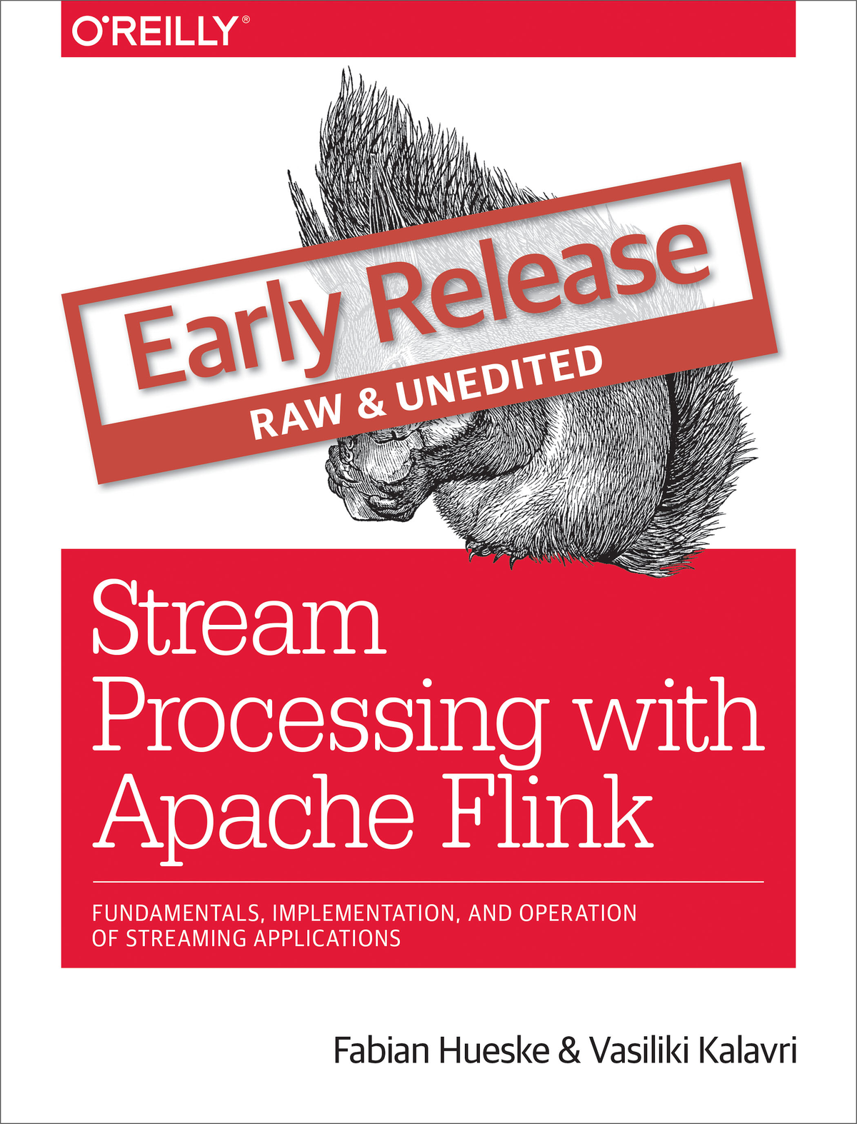
Companies employ many different applications to run their business, such as enterprise resource planning (ERP) systems, customer relationship management (CRM) software, or web-based applications. All of these systems are typically designed with separate tiers for data processing (the application itself) and data storage (a transactional database system) as shown in Figure 1-1.
The applications are usually connected to external services or face human users and continuously process incoming events such as orders, or mails, or clicks on a website. When an event is processed, an application reads its state or updates its state by running transactions against the remote database system. Typically, a database system serves multiple applications which often even access the same databases or tables.
This design can cause problems when applications need to evolve or scale. Since, multiple applications might work on the same data representation or share the same infrastructure, changing the schema of a table or scaling a database system requires careful planning and a lot of effort. A recent approach to overcome the tight bundling of applications is the microservice design pattern. Microservices are designed as small, self-contained, and independent applications. They follow the UNIX philosophy of doing a single thing and doing it well. More complex applications are built by connecting several microservices with each other that only communicate over standardized interfaces such as RESTful HTTP connections. Because microservices are strictly decoupled from each other and only communicate over well defined interfaces, each microservice can be implemented with a custom technology stack including programming language, libraries, and data stores. Microservices and all required software and services are typically bundled and deployed in independent containers. Figure 1-2 depicts a microservice architecture.
The data that is stored in the various transactional database systems of a company can provide valuable insights about various aspects of the company’s business. For example, the data of an order processing system can be analyzed to obtain sales growth over time, to identify reasons for delayed shipments, or to predict future sales in order to adjust the inventory. However, transactional data is often distributed across several disconnected database systems and becomes more valuable when it can be jointly analyzed. Moreover, it is often required to transform the data into a common format.
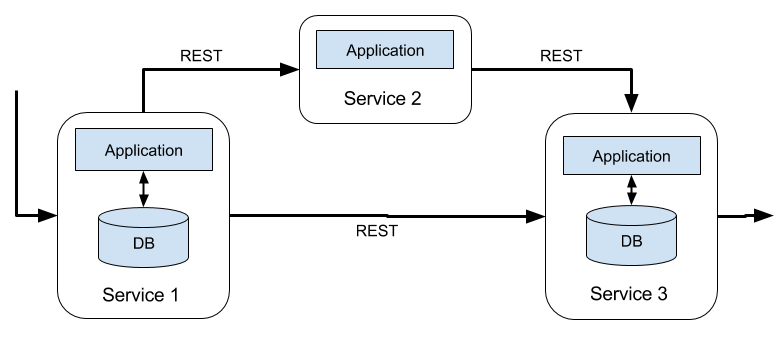
Instead of running analytical queries directly on the transactional databases, a common component in IT systems is a data warehouse. A data warehouse is a specialized database system for analytical query workloads. In order to populate a data warehouse, the data managed by the transactional database systems needs to be copied to it. The process of copying data to the data warehouse is called extract-transform-load (ETL). An ETL process extracts data from a transactional database, transforms it into a common representation which might include validation, value normalization, encoding, de-duplication, and schema transformation, and finally loads it into the analytical database. ETL processes can be quite complex and often require technically sophisticated solutions to meet performance requirements. In order to keep the data of the data warehouse up-to-date, ETL processes need to run periodically.
Once the data has been imported into the data warehouse it can be queried and analyzed. Typically, there are two classes of queries executed on a data warehouse. The first type are periodic report queries that compute business relevant statistics such as revenue, user growth, or production output. These metrics are assembled into reports that help to assess the situation of the business. The second type are ad-hoc queries that aim to provide answers to specific questions and support business-critical decisions. Both kinds of queries are executed by a data warehouse in a batch processing fashion, i.e., the data input of a query is fully available and the query terminates after it returned the computed result. The architecture is depicted in Figure 1-3.
Until the rise of Apache Hadoop, specialized analytical database systems and data warehouses were the predominant solutions for data analytics workloads. However, with the growing popularity of Hadoop, companies realized that a lot of valuable data was excluded from their data analytics process. Often, this data was either unstructured, i.e., not strictly following a relational schema, or too voluminous to be cost-effectively stored in a relational database system. Today, components of the Apache Hadoop ecosystem are integral parts in the IT infrastructures of many enterprises and companies. Instead of inserting all data into a relational database system, significant amounts of data, such as, log files, social media, or web click logs, are written into Hadoop’s distributed file system (HDFS) or other bulk data stores, like Apache HBase, which provide massive storage capacity at small cost. Data that resides in such storage systems is accessible to several SQL-on-Hadoop engines, as for example Apache Hive, Apache Drill, or Apache Impala. However, also with storage systems and execution engines of the Hadoop ecosystem the overall mode of operation of the infrastructure remains basically the same as the traditional data warehouse architecture, i.e., data is periodically extracted and loaded into to a data store and processed by periodic or ad-hoc queries in a batch fashion.
An important observation is that virtually all data is created as continuous streams of events. Think of user interactions on websites or in mobile apps, placements of orders, server logs, or sensor measurements; all of these data are streams of events. In fact, it is difficult to find examples of finite, complete data sets that are generated all at once. Stateful stream processing is an application design pattern for processing unbounded streams of events and is applicable to many different use cases in the IT infrastructure of a company. Before we discuss its use cases, we briefly explain what stateful stream processing is and how it works.
Any application that processes a stream of events and does not just perform trivial record-at-a-time transformations needs to be stateful, i.e., have the ability to store and access intermediate data. When an application receives an event, it can perform arbitrary computations that involve reading data from or writing data to the state. In principle, state can be stored and accessed in many different places including program variables, local files, or embedded or external databases.
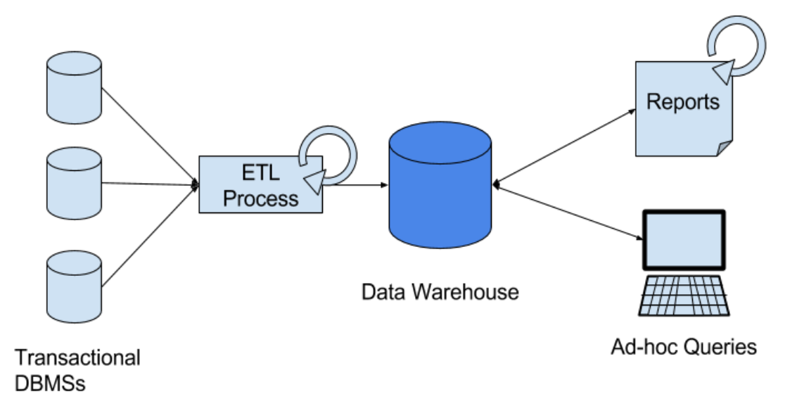
Apache Flink stores application state locally in memory or in an embedded database and not in a remote database. Since Flink is a distributed system, the local state needs to be protected against failures to avoid data loss in case of application or machine failures. Flink guarantees this by periodically writing a consistent checkpoint of the application state to a remote and durable storage. State, state consistency, and Flink’s checkpointing mechanism will be discussed in more detail in the following chapters. Figure 1-4 shows a stateful Flink application.
Stateful stream processing applications often ingest their incoming events from an event log. An event log stores and distributes event streams. Events are written to a durable, append-only log which means that the order of written events cannot be changed. A stream that is written to an event log can be read many times by the same or different consumers. Due to the append-only property of the log, events are always published to all consumers in exactly the same order. There are several event log systems available as open source software, Apache Kafka being the most popular, or as integrated services offered by cloud computing providers.
Connecting a stateful streaming application running on Flink and an event log is interesting for multiple reasons. In this architecture the event log acts as a source of truth because it persists the input events and can replay them in an deterministic order. In case of a failure, Flink restores a stateful streaming application by recovering its state from a previously taken checkpoint and resets the read position on the event log.The application will replay (and fast forward) the input events from the event log until it reaches the tail of the stream. This technique is used to recover from failures but can also be leveraged to update an application, fix bugs and repair previously emitted results, migrate an application to a different cluster, or perform A/B tests with different application versions.
As previously stated, stateful streaming processing is a versatile and flexible design pattern and can be used to address many different use cases. In the following we present three classes of applications that are commonly implemented using stateful stream processing, 1) event-driven applications, 2) data pipeline applications, and 3) data analytics applications and give examples of real-world applications. We describe these classes as distinct patterns to emphasize the versatility of stateful stream processing. However, most real-world applications combine characteristics of more than one class which again shows the flexibility of this application design pattern.
Event-driven applications are stateful streaming applications that ingest event streams and apply business logic on the received events. Depending on the business logic, an event-driven application can trigger actions such as sending an alert or an email or write events to an outgoing event stream that is possibly consumed by another event-driven application.
Typical use cases for event-driven applications include
Real-time recommendations, e.g., for recommending products while customers browse on a retailer’s website,
Pattern detection or complex event processing (CEP), e.g., for fraud detection in credit card transactions, and
Anomaly detection, e.g., to detect attempts to intrude a computer network.
Event-driven applications are an evolution of the previously discussed microservices. They communicate via event logs instead of REST calls and hold application data as local state instead of writing it to and reading it from an external data store, such as a transactional database or key-value store. Figure 1-5 sketches a service architecture composed of event-driven streaming applications.
Event-driven applications are an interesting design pattern because they offer several benefits compared to the traditional architecture of separate storage and compute tiers or the popular microservice architectures. Local state accesses, i.e., reading from or writing to memory or local disk, provide very good performance compared to read and write queries against remote data stores. Scaling and fault-tolerance do not need special consideration because these aspects are handled by the stream processor. Finally, by leveraging an event log as input source the complete input of an application is reliably stored and can be deterministically replayed. This is very attractive especially in combination with Flink’s savepoint feature which can reset the state of an application to a previous consistent savepoint. By resetting the state of a (possibly modified) application and replaying the input, it is possible to fix a bug of the application and repair its effects, deploy new versions of an application without losing its state, or run what-if or A/B tests. We know of a company that decided to built the backend of a social network based on an event log and event-driven applications because of these features.
Event-driven applications have quite high requirements on the stream processor that runs them. The business logic is constrained by how much it can control state and time. This aspect depends on the APIs of the stream processor, what kinds of state primitives it provides, and on the quality of its support for event-time processing. Moreover, exactly-once state consistency and the ability to scale an application are fundamental requirements. Apache Flink checks all these boxes and is a very good choice to run event-driven applications.
Today’s IT architectures include many different data stores, such as relational and special-purpose database systems, event logs, distributed file systems, in-memory caches, and search indexes. All of these systems store data in different representations and data structures that provide the best performance for their specific purpose. Subsets of an organization’s data are stored in multiple of these systems. For example, information for a product that is offered in a webshop can be stored in a transactional database, a web cache, and a search index. Due to this replication of data, the data stores must be kept in sync.
The traditional approach of a periodic ETL job to move data between storage systems is typically not able to propagate updates fast enough. Instead a common approach is to write all changes into an event log that serves as source of truth. The event log publishes the changes to consumers that incorporate the updates into the affected data stores. Depending on the use case and data store, the updates need to be processed before they can be incorporated. For example they need to be normalized, joined or enriched with additional data, or pre-aggregated, i.e., transformations that are also commonly performed by ETL processes.
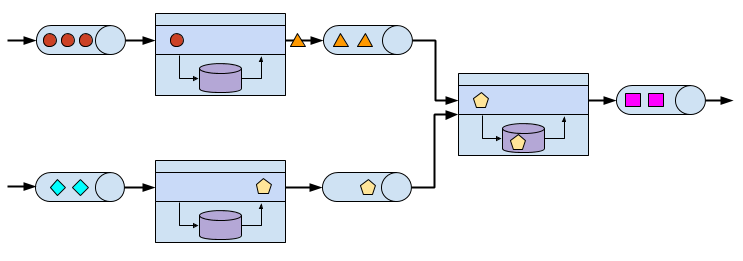
Ingesting, transforming, and inserting data with low latency is another common use case for stateful stream processing applications. We call this type of applications data pipelines. Additional requirements for data pipelines are the ability to process large amounts of data in short time, i.e., support for high throughput, and the capability to scale an application. A stream processor that operates data pipelines should also feature many source and sink connectors to read data from and write data to various storage systems and formats. Again, Flink provides all required features to successfully operate data pipelines and includes many connectors.
Previously in this chapter, we described the common architecture for data analytics pipelines. ETL jobs periodically import data into a data store and the data is processed by ad-hoc or scheduled queries. The fundamental mode of operation - batch processing - is the same regardless whether the architecture is based on a data warehouse or components of the Hadoop ecosystem. While the approach of periodically loading data into data analysis systems has been the state-of-the-art for many years, it suffers from a notable drawback.
Obviously, the periodic nature of the ETL jobs and reporting queries induce a considerable latency. Depending on the scheduling intervals it may take hours or days until a data point is included in a report. To some extent, the latency can be reduced by importing data into the data store with data pipeline applications. However, even with continuous ETL there will always be a certain delay until an event is processed by a query. In the past, analyzing data with a few hours or even days delay was often acceptable because a prompt reaction to new results or insights did not yield a significant advantage. However, this has dramatically changed in the last decade. The rapid digitalization and emergence of connected systems made it possible to collect much more data in real-time and immediately act on this data for example by adjusting to changing conditions or by personalizing user experiences. An online retailer is able to recommend products to users while they are browsing on the retailer’s website; mobile games can give virtual gifts to users to keep them in a game or offer in-game purchases at the right moment; manufacturers can monitor the behavior of machines and trigger maintenance actions to reduce production outages. All these use cases require collecting real-time data, analyzing it with low latency, and immediately reacting to the result. Traditional batch oriented architectures are not able to address such use cases.
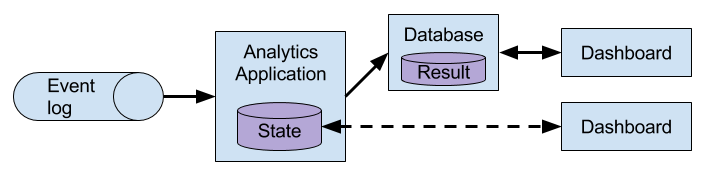
You are probably not surprised that stateful stream processing is the right technology to build low-latency analytics pipelines. Instead of waiting to be periodically triggered, a streaming analytics application continuously ingests streams of events and maintains an updating result by incorporating the latest events with low latency. This is similar to view maintenance techniques that database systems use to update materialized views. Typically, streaming applications store their result in an external data store that supports efficient updates, such as a database or key-value store. Alternatively, Flink provides a feature called queryable state which allows users to expose the state of an application as a key-lookup table and make it accessible for external applications. The live updated results of a streaming analytics applications can be used to power dashboard applications as shown in Figure 1-6.
Besides the much smaller time for an event to be incorporated into an analytics result, there is another, less obvious, advantage of streaming analytics applications. Traditional analytics pipelines consist of several individual components such as an ETL process, a storage system, and in case of a Hadoop-based environment also a data processor and scheduler to trigger jobs or queries. These components need to be carefully orchestrated and especially error handling and failure recovery can become challenging.
In contrast, a stream processor that runs a stateful streaming application takes care of all processing steps, including event ingestion, continuous computation including state maintenance, and updating the result. Moreover, the stream processor is responsible to recover from failures with exactly-once state consistency guarantees and should be capable of adjusting the parallelism of an application. Additional requirements to successfully support streaming analytics applications are support for event-time processing in order to produce correct and deterministic results and the ability to process large amounts of data in little time, i.e., high throughput. Flink offers good answers to all of these requirements.
Typical use cases for streaming analytics applications are
Monitoring the quality of cellphone networks.
Analyzing user behavior in mobile applications.
Ad-hoc analysis of live data in consumer technology.
Although not being covered in this book but certainly worth mentioning is that Flink also provides support for analytical SQL queries over streams. Multiple companies have built streaming analytics services based on Flink’s SQL support both for internal use or to publicly offer them to paying customers.
Data stream processing is not a novel technology. First research prototypes and commercial products date back to the late 1990s. However, the growing adoption of stream processing technology in the recent past is driven to a large extent by the availability of mature open source stream processors. Today, distributed open source stream processors power business-critical applications in many enterprises across different industries such as (online) retail, social media, telecommunication, gaming, and banking. Open source software is a major driver of this trend, mainly due to two reasons.
The Apache Software Foundation alone is the home of more than a dozen projects that are related to stream processing. New distributed stream processing projects are continuously entering the open source stage and are challenging the state-of-the-art with new features and capabilities. Often are features of these newcomers being adopted by more stream processors of earlier generations. Moreover, users of open source software request or contribute new features that are missing to support their use cases. This way, open source communities are constantly improving the capabilities of their projects and are pushing the technical boundaries of stream processing further. We will take a brief look into the past to see where open source stream processing came from and where it is today.
The first generation of distributed open source stream processors that got substantial adoption focused on event processing with millisecond latencies and provided guarantees that events would never be lost in case of a failure. These systems had rather low-level APIs and did not provide built-in support for accurate and consistent results of streaming applications because the results depended on the timing and order of arriving events. Moreover, even though events would not be lost in case of a failure, they could be processed more than once. In contrast to batch processors that guarantee accurate results, the first open source stream processors traded result accuracy for much better latency. The observation that data processing systems (at this point in time) could either provide fast or accurate results led to the design of the so-called Lambda architecture which is depicted in Figure 1-7.
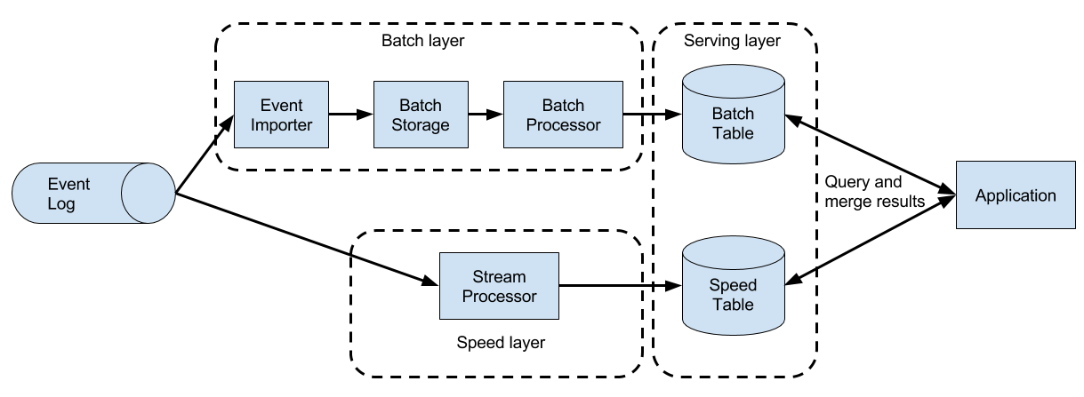
The Lambda architecture augments the traditional periodic batch processing architecture with a Speed Layer that is powered by a low-latency stream processor. Data arriving to the Lambda architecture is ingested by the stream processor as well as written to a batch storage such as HDFS. The stream processor computes possibly inaccurate results in near real-time and writes the results into a speed table. The data written to the batch storage is periodically processed by a batch processor. The exact results are written into a batch table and the corresponding inaccurate results from the speed table are dropped. Applications consume the results from the Serving Layer by merging the most recent but only approximated results from the speed table and the older but accurate result from the batch table. The Lambda architecture aimed to improve the high result latency of the original batch analytics architecture. However, the approach had a few notable drawbacks. First of all, it requires two semantically equivalent implementations of the application logic for two separate processing systems with different APIs. Second, the latest results computed by the stream processor are not accurate but only approximated. Third, the Lambda architecture is hard to setup and maintain. A textbook setup consists of a stream processor, a batch processor, a speed store, a batch store, and tools to ingest data for the batch processor and scheduling batch jobs.
Improving on the first generation, the next generation of distributed open source stream processors provided better failure guarantees and ensured that in case of a failure each record contributes exactly once to the result. In addition, programming APIs evolved from rather low-level operator interfaces to high-level APIs with more built-in primitives. However, some improvements such as higher throughput and better failure guarantees came at the cost of increasing processing latencies from milliseconds to seconds. Moreover, results were still dependent on timing and order of arriving events, i.e., the results did not depend solely on the data but also on external conditions such as the hardware utilization.
The third generation of distributed open source stream processors fixed the dependency of results on the timing and order of arriving events. In combination with exactly-once failure semantics, systems of this generation are the first open source stream processors that are capable of computing consistent and accurate results. By computing results only based on the actual data, these systems are also able to process historical data in the same way as “live” data, i.e., data which is ingested as soon as it is produced. Another improvement was the dissolution of the latency-throughput trade-off. While previous stream processors only provided either high throughput or low latency, systems of the third generation are able to serve both ends of the spectrum. Stream processors of this generation made the lambda architecture obsolete.
In addition to the system properties discussed so far, such as failure tolerance, performance, and result accuracy, stream processors also continuously added new operational features. Since streaming applications are often required to run 24/7 with minimum downtime, many stream processors added features such as highly-available setups, tight integration with resource managers, such as YARN or Mesos, and the ability to dynamically scale streaming applications. Other features include support to upgrade application code or migrating a job to a different cluster or a new version of the stream processor without losing the current state of an application.
Apache Flink is a distributed stream processor of the third generation with a competitive feature set. It provides accurate stream processing with high throughput and low latency at scale. In particular the following features let it stand out:
Flink supports event-time and processing-time semantics. Event-time provides consistent and accurate results despite out-of-order events. Processing-time can be applicable for applications with very low latency requirements.
Flink supports exactly-once state consistency guarantees.
Flink achieves millisecond latencies and is able to process millions of events per second. Flink applications can be scaled to run on thousands of cores.
Flink features layered APIs with varying tradeoffs for expressiveness and ease-of-use. This book covers the DataStream API and the ProcessFunction which provide primitives for common stream processing operations, such as windowing and asynchronous operations, and interfaces to precisely control state and time. Flink’s relational APIs, SQL and the LINQ-style Table API, are not discussed in this book.
Flink provides connectors to the most commonly used storage systems such as Apache Kafka, Apache Cassandra, Elasticsearch, JDBC, Kinesis, and (distributed) file systems such as HDFS and S3.
Flink is able to run streaming applications 24/7 with very little downtime due to its highly-available setup (no single point of failure), a tight integration with YARN and Apache Mesos, fast recovery from failures, and the ability to dynamically scale jobs.
Flink allows for updating the application code of jobs and migrating jobs to different Flink clusters without losing the state of the application.
Detailed and customizable collection of system and application metrics help to identify and react to problems ahead of time.
Last but not least, Flink is also a full-fledged batch processor.
In addition to these features, Flink is a very developer-friendly framework due to its easy-to-use APIs. An embedded execution mode starts Flink applications as a single JVM process which can be used to run and debug Flink jobs within an IDE. This feature comes in handy when developing and testing Flink applications.
Next, we will guide you through the process of starting a local cluster and executing a first streaming application in order to give you a first impression of Flink. The application we are going to run converts and aggregates randomly generated temperature sensor readings by time. For this your system needs to have Java 8 (or a later version) installed. We describe the steps for a UNIX environment. If you are running Windows, we recommend to set up a virtual machine with Linux, Cygwin (a Linux environment for Windows), or the Windows Subsystem for Linux, which was introduced with Windows 10.
Go to the Apache Flink webpage flink.apache.org and download the Hadoop-free binary distribution of Apache Flink 1.4.0.
Extract the archive file
tar xvfz flink-1.4.0-bin-scala_2.11.tgz
Start a local Flink cluster
cd flink-1.4.0

	./bin/start-cluster.sh
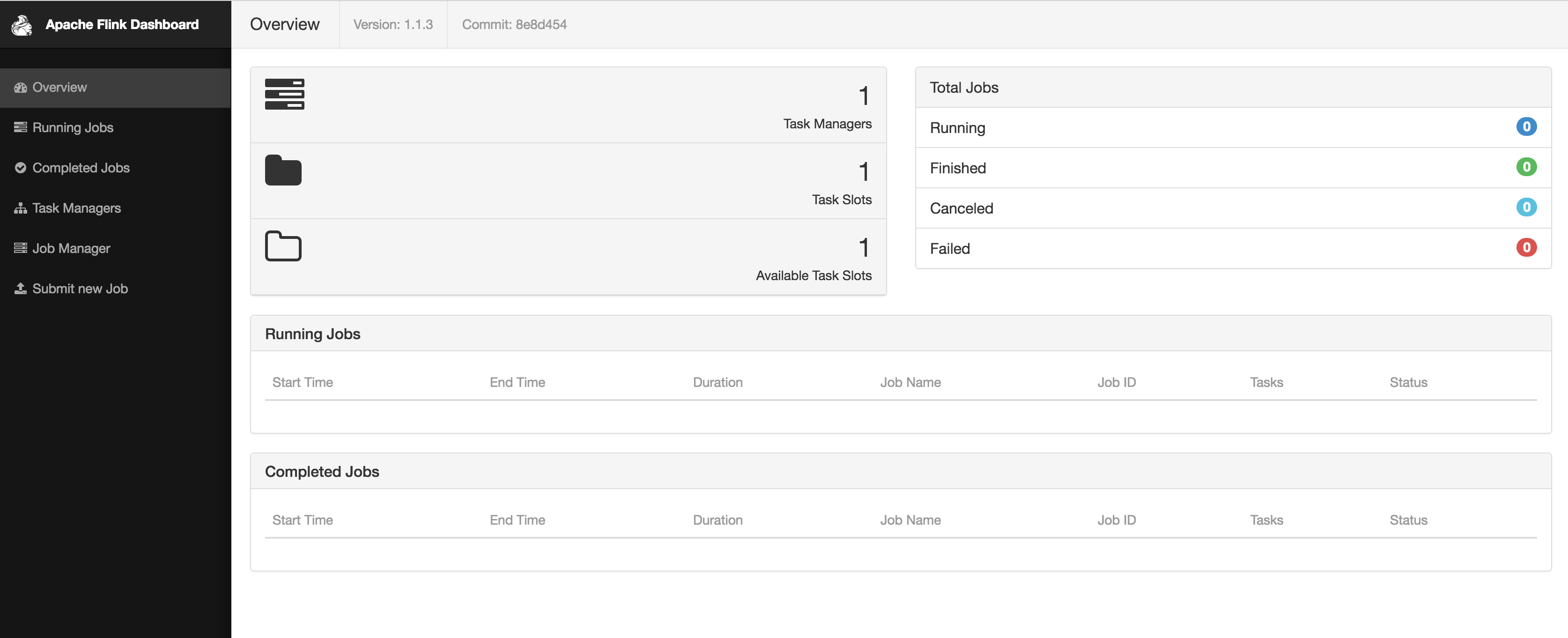
Open the web dashboard on by entering the URL http://localhost:8081 in your browser. As shown in Figure 1-8, you will see some statistics about the local Flink cluster you just started. It will show that a single Task Manager (Flink’s worker processes) is connected and that a single Task Slot (resource units provided by a Task Manager) is available.
Download the JAR file that includes all example programs of this book.
wget https://streaming-with-flink.github.io/examples/download/examples-scala.jar
Note: you can also build the JAR file yourself by following the steps on the repository’s README file.
Run the example on your local cluster by specifying the applications entry class and the JAR file
./bin/flink run -c io.github.streamingwithflink.AverageSensorReadings examples-scala.jar
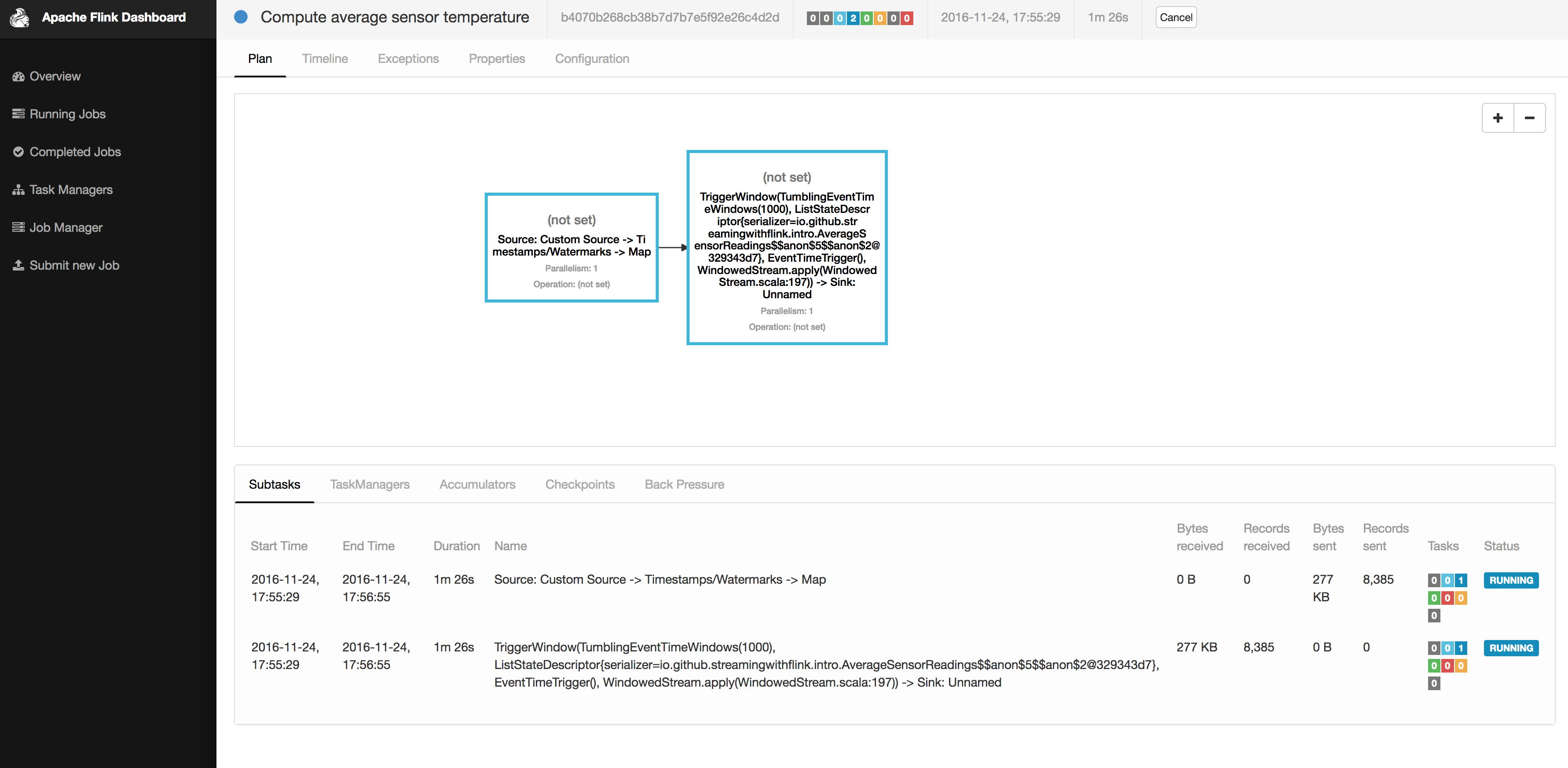
Inspect the web dashboard. You should see a job listed under “Running Jobs”. If you click on that job you will see the data flow and live metrics about the operators of the running job similar to the screenshot in Figure 1-9.
The output of the job is written to the standard out of Flink’s worker process which is by default redirected into a file in the ./log folder. You can monitor the constantly produced output using the tail command for example as follows
tail -f ./log/flink-<user>-jobmanager-<hostname>.out
You should see lines as the following ones being written to the file
SensorReading(sensor_2,1480005737000,18.832819812267438)

	SensorReading(sensor_5,1480005737000,52.416477673987856)

	SensorReading(sensor_3,1480005737000,50.83979980099426)

	SensorReading(sensor_4,1480005737000,-17.783076985394775)
The output can be read as follows: the first field of the SensorReading is a sensorId, the second field is the timestamp as milliseconds since 1970-01-01-00:00, and the third field is an average temperature computed over five seconds.
Since you are running a streaming application, it will continue to run until you cancel it. You can do this by selecting the job in the web dashboard and clicking on the CANCEL button on the top of the page.
Finally, you should stop the local Flink cluster
./bin/stop-cluster.sh
That’s it. You just installed and started your first local Flink cluster and ran your first Flink DataStream program! Of course there is much more to learn about stream processing with Apache Flink and that’s what this book is about.
This book will teach you everything to know about stream processing with Apache Flink. Chapter 2 discusses fundamental concepts and challenges of stream processing and Chapter 3 the system architecture of Flink to address these requirements. Chapters 4 to 8 guide you through setting up a development environment, cover the basics of the DataStream API, and go into the details of Flink’s time semantics and window operators, its connectors to external systems, and the details of Flink’s fault-tolerant operator state. Chapter 9 discusses how to setup and configure Flink clusters in various environments and finally Chapter 10 how to operate, monitor, and maintain streaming applications that run 24/7.
So far, you have seen how stream processing addresses limitations of traditional batch processing and how it enables new applications and architectures. You have become familiar with the evolution of the open-source stream processing space and you have got a brief taste of what a Flink streaming application looks like. In this chapter, you will enter the streaming world for good and you will get the necessary background for the rest of this book.
This chapter is still rather independent of Flink. Its goal is to introduce the fundamental concepts of stream processing and discuss the requirements of stream processing frameworks. We hope that after reading this chapter, you will have gained a better understanding of stream applications requirements and you will be able to evaluate the features of modern stream processing systems.
Before we delve into the fundamentals of stream processing, we must first introduce the necessary background on dataflow programming and establish the terminology that we will use throughout this book.
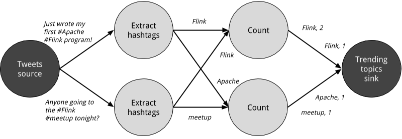
As the name suggests, a dataflow program describes how data flows between operations. Dataflow programs are commonly represented as directed graphs, where nodes are called operators and represent computations and edges represent data dependencies. Operators are the basic functional units of a dataflow application. They consume data from inputs, perform a computation on them, and produce data to outputs for further processing. Operators without input ports are called data sources and operators without output ports are called data sinks. A dataflow graph must have at least one data source and one data sink. Figure 2.1 shows a dataflow program that extracts and counts hashtags from an input stream of tweets.

Dataflow graphs like the one of Figure 2.1 are called logical because they convey a high-level view of the computation logic. In order to execute a dataflow program, its logical graph is converted into a physical dataflow graph, which includes details about how the computation is going to be executed. For instance, if we are using a distributed processing engine, each operator might have several parallel tasks running on different physical machines. Figure 2.2 shows a physical dataflow graph for the logical graph of Figure 2.1. While in the logical dataflow graph the nodes represent operators, in the physical dataflow, the nodes are tasks. The “Extract hashtags” and “Count” operators have two parallel operator tasks, each performing a computation on a subset of the input data.
You can exploit parallelism in dataflow graphs in different ways. First, you can partition your input data and have tasks of the same operation execute on the data subsets in parallel. This type of parallelism is called data parallelism. Data parallelism is useful because it allows for processing large volumes of data and spreading the computation load across several computing nodes. Second, you can have tasks from different operators performing computations on the same or different data in parallel. This type of parallelism is called task parallelism. Using task parallelism you can better utilize the computing resources of a cluster.
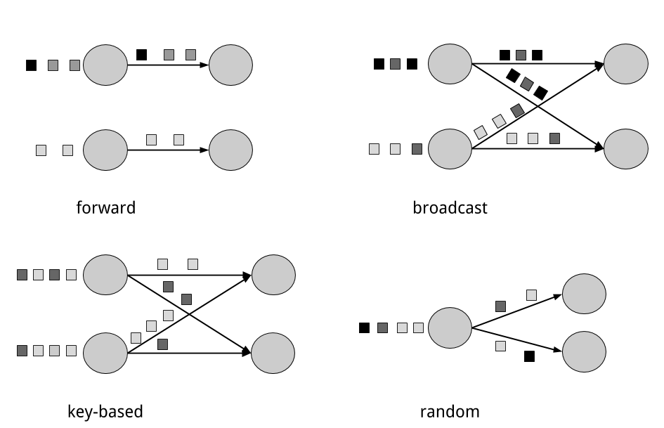
Data exchange strategies define how data items are assigned to tasks in a physical dataflow graph. Data exchange strategies can be automatically chosen by the execution engine depending on the semantics of the operators or explicitly imposed by the dataflow programmer. Here, we briefly review some common data exchange strategies, as shown in Figure 2.3.
The forward strategy and the random strategy can also be viewed as variations of the key-based strategy, where the first preserves the key of the upstream tuple while the latter performs a random re-assignment of keys.
Now that you have become familiar with the basics of dataflow programming, it’s time to see how these concepts apply to processing data streams in parallel. But first, we define the term data stream:
A data stream is a potentially unbounded sequence of events
Events in a data stream can represent monitoring data, sensor measurements, credit card transactions, weather station observations, online user interactions, web searches, etc. In this section, you are going to learn the concepts of processing infinite streams in parallel, using the dataflow programming paradigm.
In the previous chapter, you saw how streaming applications have different operational requirements from traditional batch programs. Requirements also differ when it comes to evaluating performance. For batch applications, we usually care about the total execution time of a job, or how long it takes for our processing engine to read the input, perform the computation, and write back the result. Since streaming applications run continuously and the input is potentially unbounded, there is no notion of total execution time in data stream processing. Instead, streaming applications must provide results for incoming data as fast as possible while being able to handle high ingest rates of events. We express these performance requirements in terms of latency and throughput.
Latency indicates how long it takes for an event to be processed. Essentially, it is the time interval between receiving an event and seeing the effect of processing this event in the output. To understand latency intuitively, consider your daily visit to your favorite coffee shop. When you enter the coffee shop, there might be other customers inside already. Thus, you wait in line and when it is your turn you make an order. The cashier receives your payment and passes your order to the barista who prepares your beverage. Once your coffee is ready, the barista calls your name and you can pick up your coffee from the bench. Your service latency is the time you spend in the coffee shop, from the moment you enter until you have the first sip of coffee.
In data streaming, latency is measured in units of time, such as milliseconds. Depending on the application, you might care about average latency, maximum latency, or percentile latency. For example, an average latency value of 10ms means that events are processed within 10ms on average. Instead, a 95th-percentile latency value of 10ms means that 95% of events are processed within 10ms. Average values hide the true distribution of processing delays and might make it hard to detect problems. If the barista runs out of milk right before preparing your cappuccino, you will have to wait until they bring some from the supply room. While you might get annoyed by this delay, most other customers will still be happy.
Ensuring low latency is critical for many streaming applications, such as fraud detection, raising alarms, network monitoring, and offering services with strict service level agreements (SLAs). Low latency is a key characteristic of stream processing and it enables what we call real-time applications. Modern stream processors, like Apache Flink, can offer latencies as low as a few milliseconds. In contrast, traditional batch processing latencies typically range from a few minutes to several hours. In batch processing you first need to gather the events in batches and only then you are able to process them. Thus, the latency is bounded by the arrival time of the last event in each batch and naturally depends on the batch size. True stream processing does not introduce such artificial delays and therefore can achieve really low latencies. In a true streaming model, events can be processed as soon as they arrive in the system and latency more closely reflects the actual work that has to performed on each event.
Throughput is a measure of the system’s processing capacity, i.e. its rate of processing. That is, throughput tells us how many events the system can process per time unit. Revisiting the coffee shop example, if the shop is open from 7am to 7pm and it serves 600 customers in one day, then its average throughput would be 50 customers per hour. While you want latency to be as low as possible, you generally want throughput to be as high as possible.
Throughput is measured in events or operations per time unit. It is important to note that the rate of processing depends on the rate of arrival; low throughput does not necessarily indicate bad performance. In streaming systems you usually want to ensure that your system can handle the maximum expected rate of events. That is, you are primarily concerned with determining the peak throughput, i.e. the performance limit when your system is at its maximum load. To better understand the concept of peak throughput, let us consider that system resources are completely unused. As the first event comes in, it will be immediately processed with the minimum latency possible. If you are the first customer showing up at the coffee shop right after it opened its doors in the morning, you will be served immediately. Ideally, you would like this latency to remain constant and independent of the rate of the incoming events. However, once we reach a rate of incoming events such that the system resources are fully used, we will have to start buffering events. In the coffee shop example, you will probably see this happening right after lunch. Many people show up at the same time and you have to wait in line to place your order. At this point the system has reached the peak throughput and further increasing the event rate will only result in worse latency. If the system continues to receive data at a higher rate than it can handle, buffers might become unavailable and data might get lost. This situation is commonly known as backpressure and there exist different strategies to deal with it. In Chapter 3, we look at Flink’s backpressure mechanism in detail.
At this point, it should be quite clear that latency and throughput are not independent metrics. If events take long to travel in the data processing pipeline, we cannot easily ensure high throughput. Similarly, if a system’s capacity is small, events will be buffered and have to wait before they get processed.
Let us revisit the coffee shop example to clarify how latency and throughput affect each other. First, it should be clear that there is an optimal latency in the case of no load. That is, you will get the fastest service if you are the only customer in the coffee shop. However, during busy times, customers will have to wait in line and latency will increase. Another factor that affects latency and consequently throughput is the time it takes to process an event, or the time it takes for each customer to be served in the coffee shop. Imagine that during Christmas holiday season, baristas have to draw a Santa Claus on the cup of each coffee they serve. This way, the time to prepare a single beverage will increase, causing each person to spend more time in the coffee shop, thus lowering the overall throughput.
Then, can you somehow get both low latency and high throughput or is this a hopeless endeavour? One way you can lower latency is by hiring a more skilled barista, i.e. one that prepares coffees faster. At high load, this change will also increase throughput, because more customers will be served in the same amount of time. Another way to achieve the same result is to hire a second barista, that is, to exploit parallelism. The main take-away here is that lowering latency actually increases throughput. Naturally, if a system can perform operations faster, it can perform more operations at the same amount of time. In fact, that is what you achieve by exploiting parallelism in a stream processing pipeline. By processing several streams in parallel, you can lower the latency while processing more events at the same time.
Stream processing engines usually provide a set of built-in operations to ingest, transform, and output streams. These operators can be combined into dataflow processing graphs to implement the logic of streaming applications. In this section, we describe the most common streaming operations.
Operations can be either stateless or stateful. Stateless operations do not maintain any internal state. That is, the processing of an event does not depend on any events seen in the past and no history is kept. Stateless operations are easy to parallelize, since events can be processed independently of each other and of their arriving order. Moreover, in the case of a failure, a stateless operator can be simply restarted and continue processing from where it left off. On the contrary, stateful operators may maintain information about the events they have received before. This state can be updated by incoming events and can be used in the processing logic of future events. Stateful stream processing applications are more challenging to parallelize and operate in a fault tolerant manner because state needs to be efficiently partitioned and reliably recovered in the case of failures. You will learn more about stateful stream processing, failure scenarios, and consistency in the end of this chapter.
Data ingestion and data egress operations allow the stream processor to communicate with external systems. Data ingestion is the operation of fetching raw data from external sources and converting it into a format that is suitable for processing. Operators that implement data ingestion logic are called data sources. A data source can ingest data from a TCP socket, a file, a Kafka topic, or a sensor data interface. Data egress is the operation of producing output in a form that is suitable for consumption by external systems. Operators that perform data egress are called data sinks and examples include files, databases, message queues, and monitoring interfaces.
Transformation operations are single-pass operations that process each event independently. These operations consume one event after the other and apply some transformation to the event data, producing a new output stream. The transformation logic can be either integrated in the operator or provided by a user-defined function (UDF), as shown in Figure 2.4. UDFs are written by the application programmer and implement custom computation logic.

Operators can accept multiple inputs and produce multiple output streams. They can also modify the structure of the dataflow graph by either splitting a stream into multiple streams or merging streams into a single flow. We discuss the semantics of all operators available in Flink in Chapter 5.
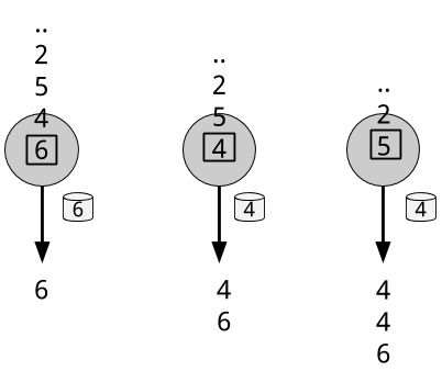
A rolling aggregation is an aggregation, such as sum, minimum, and maximum, that is continuously updated for each input event. Aggregation operations are stateful and combine the current state with the incoming event to produce an updated aggregate value. Note that to be able to efficiently combine the current state with an event and produce a single value, the aggregation function must be associative and commutative. Otherwise, the operator would have to store the complete stream history. Figure 2.5 shows a rolling minimum aggregation. The operator keeps the current minimum value and accordingly updates it for each incoming event.
Transformations and rolling aggregations process one event at a time to produce output events and potentially update state. However, some operations must collect and buffer records to compute their result. Consider for example a streaming join operation or a holistic aggregate, such as median. In order to evaluate such operations efficiently on unbounded streams, you need to limit the amount of data these operations maintain. In this section, we discuss window operations, which provide such a mechanism.
Apart from having a practical value, windows also enable semantically interesting queries on streams. You have seen how rolling aggregations encode the history of the whole stream in an aggregate value and provide us with a low-latency result for every event. This is fine for some applications, but what if you are only interested in the most recent data? Consider an application that provides real-time traffic information to drivers so that they can avoid congested routes. In this scenario, you want to know if there has been an accident in a certain location within the last few minutes. On the other hand, knowing about all accidents that have ever happened might not be so interesting in this case. What’s more, by reducing the stream history to a single aggregate, you lose the information about how your data varies over time. For instance, you might want to know how many vehicles cross an intersection every 5 minutes.
Window operations continuously create finite sets of events called buckets from an unbounded event stream and let us perform computations on these finite sets. Events are usually assigned to buckets based on data properties or based on time. To properly define window operator semantics, we need to answer two main questions: “how are events assigned to buckets?” and “how often does the window produce a result?”. The behavior of windows is defined by a set of policies. Window policies decide when new buckets are created, which events are assigned to which buckets, and when the contents of a bucket get evaluated. The latter decision is based on a trigger condition. When the trigger condition is met, the bucket contents are sent to an evaluation function that applies the computation logic on the bucket elements. Evaluation functions can be aggregations like sum or minimum or custom operations applied on the bucket’s collected elements. Policies can be based on time (e.g. events received in the last 5 seconds), on count (e.g. the last 100 events), or on a data property. In this section, we describe the semantics of common window types.

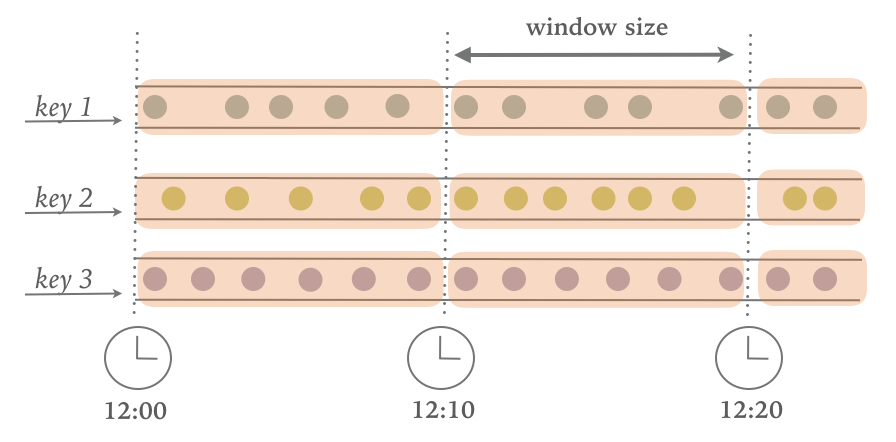


All the window types that you have seen so far are global windows and operate on the full stream. In practice though you might want to partition a stream into multiple logical streams and define parallel windows. For instance, if you are receiving measurements from different sensors, you probably want to group the stream by sensor id before applying a window computation. In parallel windows, each partition applies the window policies independently of other partitions. Figure 2.10 shows a parallel count-based tumbling window of length 2 which is partitioned by event color.

Window operations are closely related to two dominant concepts in stream processing: time semantics and state management. Time is perhaps the most important aspect of stream processing. Even though low latency is an attractive feature of stream processing, its true value is way beyond just offering fast analytics. Real-world systems, networks, and communication channels are far from perfect, thus streaming data can often be delayed or arrive out-of-order. It is crucial to understand how you can deliver accurate and deterministic results under such conditions. What’s more, streaming applications that process events as they are produced should also be able to process historical events in the same way, thus enabling offline analytics or even time travel analyses. Of course, none of this matters if your system cannot guard state against failures. All the window types that you have seen so far need to buffer data before performing an operation. In fact, if you want to compute anything interesting in a streaming application, even a simple count, you need to maintain state. Considering that streaming applications might run for several days, months, or even years, you need to make sure that state can be reliably recovered under failures and that your system can guarantee accurate results even if things break. In the rest of this chapter, we are going to look deeper into the concepts of time and state guarantees under failures in data stream processing.
In this section, we introduce time semantics and describe the different notions of time in streaming. We discuss how a stream processor can provide accurate results with out-of-order events and how you can perform historical event processing and time travel with streaming.
When dealing with a potentially unbounded stream of continuously arriving events, time becomes a central aspect of applications. Let’s assume you want to compute results continuously, for example every one minute. What would one minute really mean in the context of our streaming application?
Consider a program that analyzes events generated by users playing online mobile games. Users are organized in teams and the application collects a team’s activity and provides rewards in the game, such as extra lives and level-ups, based on how fast the team’s members meet the game’s goals. For example, if all users in a team pop 500 bubbles within one minute, they get a level-up. Alice is a devoted player who plays the game every morning during her commute to work. The problem is that Alice lives in Berlin and she takes the subway to work. And everyone knows that the mobile internet connection in the Berlin subway is lousy. Consider the case where Alice starts popping bubbles while her phone is connected to the network and sends events to the analysis application. Then suddenly, the train enters a tunnel and her phone gets disconnected. Alice keeps on playing and the game events are buffered in her phone. When the train exits the tunnel, she comes back online, and pending events are sent to the application. What should the application do? What’s the meaning of one minute in this case? Does it include the time Alice was offline or not?
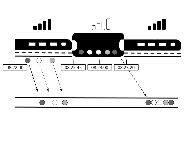
Online gaming is a simple scenario showing how operator semantics should depend on the time when events actually happen and not the time when the application receives the events. In the case of a mobile game, consequences can be as bad as Alice and her team getting disappointed and never playing again. But there are much more time-critical applications whose semantics we need to guarantee. If we only consider how much data we receive within one minute, our results will vary and depend on the speed of the network connection or the speed of the processing. Instead, what really defines the amount of events in one minute is the time of the data itself.
In Alice’s game example, the streaming application could operate with two different notions of time, Processing time or Event time. We describe both notions in the following sections.
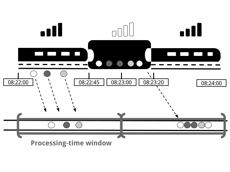
Processing time is the time of the local clock on the machine where the operator processing the stream is being executed. A processing-time window includes all events that happen to have arrived at the window operator within a time period, as measured by the wall-clock of its machine. As shown in Figure 2-12, in Alice’s case, a processing-time window would continue counting time when her phone gets disconnected, thus not accounting for her game activity during that time.
Event-time is the time when an event in the stream actually happened. Event time is based on a timestamp that is attached on the events of the stream. Timestamps usually exist inside the event data before they enter the processing pipeline (e.g. event creation time). Figure 2-13 shows that an event-time window would correctly place events in a window, reflecting the reality of how things happened, even though some events were delayed.
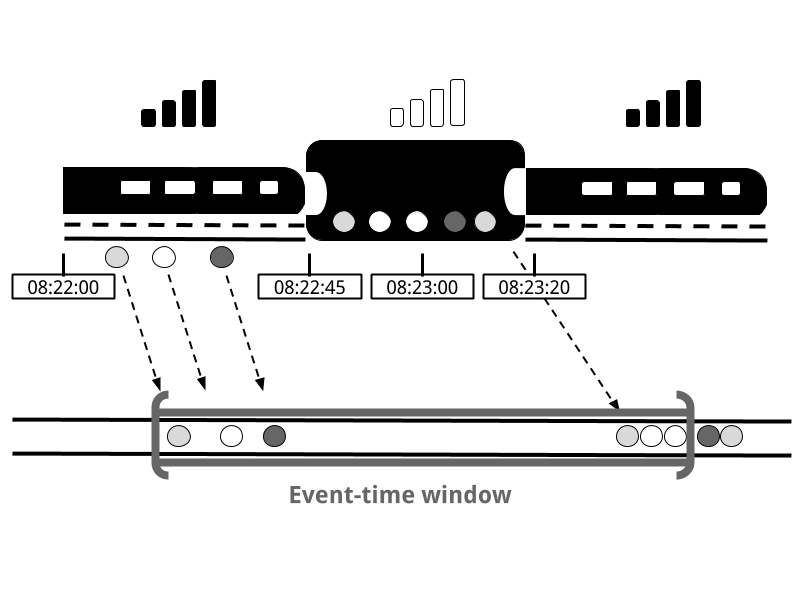
Event-time completely decouples the processing speed from the results. Operations based on event-time are predictable and their results deterministic. An event-time window computation will yield the same result no matter how fast the stream is processed or when the events arrive at the operator.
Handling delayed events is only one of the challenges that you can overcome with event time. Except from experiencing network delays, streams might be affected by many other factors resulting in events arriving out-of-order. Consider Bob, another player of the online mobile game, who happens to be on the same train as Alice. Bob and Alice play the same game but they have different mobile providers. While Alice’s phone loses connection when inside the tunnel, Bob’s phone remains connected and delivers events to the gaming application.
By relying on event time, we can guarantee result correctness even in such cases. What’s more, when combined with replayable streams, the determinism of timestamps gives you the ability to fast-forward the past. That is, you can re-play a stream and analyze historic data as if events are happening in real-time. Additionally, you can fast-forward the computation to the present so that once your program catches up with the events happening now, it can continue as a real-time application using exactly the same program logic.
In our discussion about event-time windows so far, we have overlooked one very important aspect: how do we decide when to trigger an event-time window? That is, how long do we have to wait before we can be certain that we have received all events that happened before a certain point of time? And how do we even know that data will be delayed? Given the unpredictable reality of distributed systems and arbitrary delays that might be caused by external components, there is no categorically correct answer to these questions. In this section, we will see how we can use the concept of watermarks to configure event-time window behavior.
A watermark is a global progress metric that indicates a certain point in time when we are confident that no more delayed events will arrive. In essence, watermarks provide a logical clock which informs the system about the current event time. When an operator receives a watermark with time T, it can assume that no further events with timestamp less than T will be received. Watermarks are essential to both event-time windows and operators handling out-of-order events. Once a watermark has been received, operators are signaled that all timestamps for a certain time interval have been observed and either trigger computation or order received events.
Watermarks provide a configurable trade-off between results confidence and latency. Eager watermarks ensure low latency but provide lower confidence. In this case, late events might arrive after the watermark and we should provide some code to handle them. On the other hand, if watermarks are too slow to arrive, you have high confidence but you might unnecessarily increase processing latency.
In many real-world applications, the system does not have enough knowledge to perfectly determine watermarks. In the mobile gaming case for example, it is practically impossible to know for how long a user might remain disconnected; they could be going through a tunnel, boarding a plane, or never playing again. No matter if watermarks are user-defined or automatically generated, tracking global progress in a distributed system might be problematic in the presence of straggler tasks. Hence, simply relying on watermarks might not always be a good idea. Instead, it is crucial that the stream processing system provides some mechanism to deal with events that might arrive after the watermark. Depending on the application requirements, you might want to ignore such events, log them, or use them to correct previous results.
At this point, you might be wondering: Since event time solves all of our problems, why even bother considering processing time? The truth is that processing time can indeed be useful in some cases. Processing-time windows introduce the lowest latency possible. Since you do not take into consideration late events and out-of-order events, a window simply needs to buffer up events and immediately trigger computation once the specified time length is reached. Thus, for applications where speed is more important than accuracy, processing time comes handy. Another case is when you need to periodically report results in real-time, independently of their accuracy. An example application would be a real-time monitoring dashboard that displays event aggregates as they are received. Finally, processing time windows offer a faithful representation of the streams themselves, might also be a desirable property for some use-cases. To recap, processing time offers low latency but results depend on the speed of processing and are not deterministic. On the other hand, event time guarantees deterministic results and allows you to deal with events that are late or even out-of-order.
We now turn to examine another extremely important aspect of stream processing, state. State is ubiquitous in data processing. It is required by any non-trivial computation. To produce a result, a UDF accumulates state over a period or number of events, e.g. to compute an aggregation or detect a pattern. Stateful operators use both incoming events and internal state to compute their output. Take for example a rolling aggregation operator that outputs the current sum of all the events it has seen so far. The operator keeps the current value of the sum as its internal state and updates it every time it receives a new event. Similarly, consider an operator that raises an alert when it detects a “high temperature” event followed by a “smoke” event within 10 minutes. The operator needs to store the “high temperature” event in its internal state, until it sees the “smoke” event or the until 10-minute time period expires.
The importance of state becomes even more evident if we consider the case of using a batch processing system to analyze an unbounded data set. In fact, this has been a common implementation choice before the rise of modern stream processors. In such a case, a job is executed repeatedly over batches of incoming events. When the job finishes, the result is written to persistent storage, and all operator state is lost. Once the job is scheduled for execution on the next batch, it cannot access the state of the previous job. This problem is commonly solved by delegating state management to an external system, such as a database. On the contrary, with continuously running streaming jobs, manipulating state in the application code is substantially simplified. In streaming we have durable state across events and we can expose it as a first-class citizen in the programming model. Arguably, one could use an external system to also manage streaming state, even though this design choice might introduce additional latency.
Since streaming operators process potentially unbounded data, caution should be taken to not allow internal state to grow indefinitely. To limit the state size, operators usually maintain some kind of summary or synopsis of the events seen so far. Such a summary can be a count, a sum, a sample of the events seen so far, a window buffer, or a custom data structure that preserves some property interesting to the running application.
As one could imagine, supporting stateful operators comes with a few implementation challenges. First, the system needs to efficiently manage the state and make sure it is protected from concurrent updates. Second, parallelization becomes complicated, since results depend on both the state and incoming events. Fortunately, in many cases, you can partition the state by a key and manage the state of each partition independently. For example, if you are processing a stream of measurements from a set of sensors, you can use partitioned operator state to maintain state for each sensor independently. The third and biggest challenge that comes with stateful operators is ensuring that the state can be recovered and that results will be correct in the presence of failures. In the next section, you will learn about task failures and result guarantees in detail.
Operator state in streaming jobs is very valuable and should be guarded against failures. If state gets lost during a failure, results will be incorrect after recovery. Streaming jobs run for long periods of time, thus state might be collected over several days or even months. Reprocessing all input to reproduce lost state in the case of failures would be both very expensive and time-consuming.
In the beginning of this chapter, you saw how you can model streaming programs as dataflow graphs. Before execution, these are translated into physical dataflow graphs of many connected parallel tasks, each running some operator logic, consuming input streams and producing output streams for other tasks. Typical real-world setups can easily have hundreds of such tasks running in parallel on many physical machines. In long-running, streaming jobs, each of these tasks can fail at any time. How can you ensure that such failures are handled transparently so that your streaming job can continue to run? In fact, you would like your stream processor to not only continue the processing in the case of task failures, but also provide correctness guarantees about the result and operator state. We discuss all these matters in this section.
For each event in the input stream, a task performs the following steps: (1) receive the event, i.e. store it in a local buffer, (2) possibly update internal state, and (3) produce an output record. A failure can occur during any of these steps and the system has to clearly define its behavior in a failure scenario. If the task fails during the first step, will the event get lost? If it fails after it has updated its internal state, will it update it again after it recovers? And in those cases, will the output be deterministic?
We assume reliable network connections, such that no records are dropped or duplicated and all events are eventually delivered to their destination in FIFO order. Note that Flink uses TCP connections, thus these requirements are guaranteed. We also assume perfect failure detectors and that no task will intentionally act maliciously; that is, all non-failed tasks follow the above steps.
In a batch processing scenario, you can solve all these problems easily since all the input data is available. The most trivial way would be to simply restart the job, but then we would have to replay all data. In the streaming world, however, dealing with failures is not a trivial problem. Streaming systems define their behavior in the presence of failures by offering result guarantees. Next, we review the types of guarantees offered by modern stream processors and some mechanisms that systems implement to achieve those guarantees.
The simplest thing to do when a task fails is to do nothing to recover lost state and replay lost events. At-most-once is the trivial case that guarantees processing of each event at-most-once. In other words, events can be simply dropped and there is no mechanism to ensure result correctness. This type of guarantee is also known as “no-guarantee” since even a system that drops every event can fulfil it. Having no guarantees whatsoever sounds like a terrible idea, but it might be fine, if you can live with approximate results and all you care about is providing the lowest latency possible.
In most real-world applications, the minimum requirement is that events do not get lost. This type of guarantee is called at-least-once and it means that all events will definitely be processed, even though some of them might be processed more than once. Duplicate processing might be acceptable if application correctness only depends on the completeness of information. For example, determining whether a specific event occurs in the input stream can be correctly realized with at-least-once guarantees. In the worst case, you will locate the event more than once. However, counting how many times a specific event occurs in the input stream might return the wrong result under at-least-once guarantees.
In order to ensure at-least-once result correctness, you need to have a mechanism to replay events, either from the source or from some buffer. Persistent event logs write all events to durable storage, so that they can be replayed if a task fails. Another way to achieve equivalent functionality is using record acknowledgements. This method stores every event in a buffer until its processing has been acknowledged by all tasks in the pipeline, at which point the event can be discarded.
This is the strictest and most challenging to achieve type of guarantee. Exactly-once result guarantees means that not only there will be no event loss, but also updates on the internal state will be applied exactly once for each event. In essence, exactly-once guarantees mean that our application will provide the correct result, as if a failure never happened.
Providing exactly-once guarantees requires at-least-once guarantees, thus a data replay mechanism is again necessary. Additionally, the stream processor needs to ensure internal state consistency. That is, after recovery, it should know whether an event update has already been reflected on the state or not. Transactional updates is one way to achieve this result, however, it can incur substantial performance overhead. Instead, Flink uses a lightweight snapshotting mechanism to achieve exactly-once result guarantees. We discuss Flink’s fault-tolerance algorithm in Chapter 3.
The types of guarantees you have seen so far refer to the stream processor component only. In a real-word streaming architecture however, it is common to have several connected components. In the very simple case, there will be at least one source and one sink apart from the stream processor. End-to-end guarantees refer to result correctness across the data processing pipeline. To assess end-to-end guarantees, one has to consider all the components of an application pipeline. Each component provides its own guarantees and the end-to-end guarantee of the complete pipeline would be the weakest of each of its components. It is important to note that sometimes you can get stronger semantics with weaker guarantees. A common case is when a task performs idempotent operations, like maximum or minimum. In this case, you can achieve exactly-once semantics with at-least-once guarantees.
In this chapter, you have learned the fundamental concepts and ideas of data stream processing. You have seen the dataflow programming model and learned how streaming applications can be expressed as distributed dataflow graphs. Next, you have looked into the requirements of processing infinite streams in parallel and you have realized the importance of latency and throughput for stream applications. You have learned basic streaming operations and how you can compute meaningful results on unbounded input data using windows. You have wondered about the meaning of time in stream processing and you have compared the notions of event time and processing time. Finally, you have seen why state is important in streaming applications and how you can guard it against failures and guarantee correct results.
Up to this point, we have considered streaming concepts independently of Apache Flink. In the rest of this book, we are going to see how Flink actually implements these concepts and how you can use its DataStream APIs to write applications that use all of the features that we have introduced so far.
The previous chapter discussed important concepts of distributed stream processing, such as parallelization, time, and state. In this chapter we give a high-level introduction to Flink’s architecture and describe how Flink addresses the aspects of stream processing that we discussed before. In particular, we explain Flink’s process architecture and the design of its networking stack. We show how Flink handles time and state in streaming applications and discuss its fault tolerance mechanisms. This chapter provides relevant background information to successfully implement and operate advanced streaming applications with Apache Flink. It will help you to understand Flink’s internals and to reason about the performance and behavior of streaming applications.
Flink is a distributed system for stateful parallel data stream processing. A Flink setup consists of multiple processes that run distributed across multiple machines. Common challenges that distributed systems need to address are allocation and management of compute resources in a cluster, process coordination, durable and available data storage, and failure recovery.
Flink does not implement all the required functionality by itself. Instead, it focuses on its core function - distributed data stream processing - and leverages existing cluster infrastructure and services. Flink is tightly integrated with cluster resource managers, such as Apache Mesos, YARN, and Kubernetes, but can also be configured to run as a stand-alone cluster. Flink does not provide durable, distributed storage. Instead it supports distributed file systems like HDFS or object stores such as S3. For leader election in highly-available setups, Flink depends on Apache ZooKeeper.
In this section we describe the different components that a Flink setup consists of and discuss their responsibilities and how they interact with each other to execute an application. We present two different styles of deploying Flink applications and discuss how tasks are distributed and executed. Finally, we explain how Flink’s highly-available mode works.
A Flink setup consists for four different components that work together to execute streaming applications. These components are a JobManager, a ResourceManager, a TaskManager, and a Dispatcher. Since Flink is implemented in Java and Scala, all components run on a Java Virtual Machine (JVM). We discuss the responsibilities of each component and how it interacts with the other components in the following.
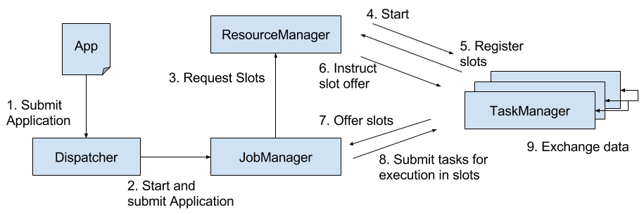
Please note that Figure 3-1 is a high-level sketch to visualize the responsibilities and interactions of the components. Depending on the the environment (YARN, Mesos, Kubernetes, stand-alone cluster), some steps can be omitted or components might run in the same process. For instance, in a stand-alone setup, i.e., a setup without a resource provider, the ResourceManager can only distribute the slots of manually started TaskManagers and cannot start new TaskManagers. In Chapter 9, we will discuss how to setup and configure Flink for different environments.
Flink applications can be deployed in two different styles.
The framework style is follows the traditional approach of submitting an application (or query) via a client to a running service. In the library mode, there is no Flink service continuously running. Instead, Flink is bundled as a library together with the application in a container image. This deployment mode is also common for microservice architectures. We discuss the topic of application deployment in more detail in Chapter 10.
A TaskManager can execute several tasks at the same time. These tasks can be of the same operator (data parallelism), a different operator (task parallelism), or even from a different application (job parallelism). A TaskManager provides a certain number of processing slots to control the number of tasks that it can concurrently execute. A processing slot is able to execute one slice of an application, i.e., one task of each operator of the application. Figure 3-2 visualizes the relationship of TaskManagers, slots, tasks, and operators.
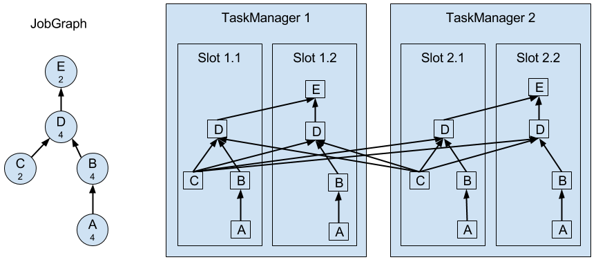
On the left hand side you see a JobGraph - the non-parallel representation of an application - consisting of five operators. Operators A and C are sources and operator E is a sink. Operators C and E have a parallelism of two. The other operators have a parallelism of four. Since the maximum operator parallelism is four, the application requires at least four available processing slots to be executed. Given two TaskManagers with two processing slots each, this requirement is fulfilled. The JobManager parallelizes the JobGraph into an ExecutionGraph and assigns the tasks to the four available slots. The tasks of the operators with a parallelism of four are assigned to each slot. The two tasks of operators C and E are assigned to slots 1.1 and 2.1 and slots 1.2 and 2.2, respectively1. Scheduling tasks as slices to slots has the advantage that many tasks are co-located on the TaskManager which means that they can efficiently exchange data without accessing the network.
A TaskManager executes its tasks multi-threaded in the same JVM process. Threads are more lightweight than individual processes and have lower communication costs but do not strictly isolate tasks from each other. Hence, a single misbehaving task can kill the whole TaskManager process and all tasks which run on the TaskManager. Therefore, it is possible to isolate applications across TaskManagers, i.e., a TaskManager runs only tasks of one application. By leveraging thread-parallelism inside of a TaskManager and the option to deploy several TaskManager processes per host, Flink offers a lot of flexibility to trade off performance and resource isolation when deploying applications. We will discuss the configuration and setup of Flink clusters in detail in Chapter 9.
Streaming applications are typically designed to run 24/7. Hence, it is important that their execution does not stop even if an involved process fails. Recovery from failures consists of two aspects, first restarting failed processes and second restarting the application and recovering its state. In this section, we explain how Flink restarts failed processes. Restoring the state of an application is discussed in a later section of this chapter.
As discussed before, Flink requires a sufficient amount of processing slots in order to execute all tasks of an application. Given a Flink setup with four TaskManagers that provide two slots each, a streaming application can be executed with a maximum parallelism of eight. If one of the TaskManagers fails, the number of available slots is reduced to six. In this situation, the JobManager will ask the ResourceManager to provide more processing slots. If this is not possible, for example because the application runs in a stand-alone cluster, the JobManager scales the application down and executes it on fewer slots until more slots become available.
A more challenging problem than TaskManager failures are JobManager failures. The JobManager controls the execution of a streaming application and keeps metadata about its execution, such as pointers to completed checkpoints. A streaming application cannot continue processing if the associated JobManager process disappears which makes the JobManager a single-point-of-failure in Flink. To overcome this problem, Flink features a high-availability mode that migrates the responsibility and metadata for a job to another JobManager in case that the original JobManager disappears.
Flink’s high-availability mode is based on Apache ZooKeeper, a system for distributed services that require coordination and consensus. Flink uses ZooKeeper for leader election and as a highly-available and durable data store. When operating in high-availability mode, the JobManager writes the JobGraph and all required metadata such as the application’s JAR file into a remote persistent storage system. In addition, the JobManager writes a pointer to the storage location into ZooKeeper’s data store. During the execution of an application, the JobManager receives the state handles (storage locations) of the individual task checkpoints. Upon the completion of a checkpoint, i.e., when all tasks have successfully written their state into the remote storage, the JobManager writes the state handles to the remote storage and a pointer to this location to ZooKeeper. Hence, all data that is required to recover from a JobManager failure is stored in the remote storage and ZooKeeper holds pointers to the storage locations. Figure 3-3 illustrates this design.
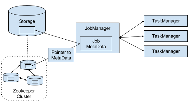
When a JobManager fails, all tasks that belong to its application are automatically cancelled. A new JobManager that takes over the work of the failed master performs the following steps.
When running an application as a library deployment in a container environment, such as Kubernetes, failed JobManager or TaskManager containers can be automatically restarted. When running on YARN or on Mesos, Flink’s remaining processes trigger the restart of JobManager or TaskManager processes. Flink does not provide tooling to restart failed processes when running in a stand-alone cluster. Hence, it can be useful to run stand-by JobManagers and TaskManager that can take over the work of failed processes. We will discuss the configuration of highly available Flink setups later in Chapter 9.
The tasks of a running application are continuously exchanging data. The TaskManagers take care of shipping data from sending tasks to receiving tasks. The network component of a TaskManager collect records in buffers before they are shipped, i.e., records are not shipped one-by-one but batched into buffers. This technique is fundamental to effectively utilize the networking resource and achieve high throughput. The mechanism is similar to buffering techniques used in networking or disk IO protocols. Note shipping records in buffers does imply that Flink’s processing model is based on micro-batches.
Each TaskManager has a pool of network buffers (by default 32KB in size) which are used to send and receive data. If the sender and receiver tasks run in separate TaskManager processes, they communicate via the network stack of the operating system. Streaming applications need to exchange data in a pipelined fashion, i.e., each pair of TaskManagers maintains a permanent TCP connection to exchange data2. In case of a shuffle connection pattern, each sender task needs to be able to send data to each receiving task. A TaskManager needs one dedicated network buffer for each receiving task that any of its tasks need to send data to. Once a buffer is filled, it is shipped over the network to the receiving task. On the receiver side, each receiving task needs one network buffer for each of its connected sending tasks. Figure 3-4 visualizes this architecture.
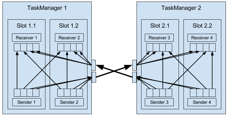
The figure shows four sender and four receiver tasks. Each sender task has four network buffers to send data to each receiver task and each receiver task has four buffers to receive data. Buffers which need to be sent to the other TaskManager are multiplexed over the same network connection. In order to enable a smooth pipelined data exchange, a TaskManager must be able to provide enough buffers to serve all outgoing and incoming connections concurrently. In case of a shuffle or broadcast connection, each sending task needs a buffer for each receiving task, i.e, the number of required buffers is quadratic to the parallelism of the involved operators.
If the sender and receiver task run in the same TaskManager process, the sender task serializes the outgoing records into a byte buffer and puts the buffer into a queue once it is filled. The receiving task takes the buffer from the queue and deserializes the incoming records. Hence, no network communication is involved. Serializing records between TaskManager-local tasks has the advantage that it decouples the tasks and allows to use mutable objects in tasks which can considerably improve the performance because it reduces object instantiations and garbage collection. Once an object has been serialized, it can be safely modified.
On the other hand, serialization can cause significant computational overhead. Therefore, Flink can - under certain conditions - chain multiple DataStream operators into a single task. Operators in the same task communicate by passing objects through nested function calls which avoids serialization. The concept of operator chaining is discussed in more detail in Chapter 10.
Sending individual records over a network connection is inefficient and causes significant overhead. Buffering is a mandatory technique to fully utilize the bandwidth of network connections. In the context of stream processing, one disadvantage of buffering is that it adds latency because records are collected in a buffer instead of being immediately shipped. If a sender task only rarely produces records for a specific receiving task, it might take a long time until the respective buffer is filled and shipped. Because this would cause high processing latencies, Flink ensures that each buffer is shipped after a certain period of time regardless of how much it is filled. This timeout can be interpreted as an upper bound for the latency added by a network connection. However, the threshold does not serve as a strict latency SLA for the job as a whole because a job might involve multiple network connections and it does also not account for delays caused by the actual processing.
Streaming applications that ingest streams with high volume can easily come to a point where a task is not able to process its input data at the rate at which it arrives. This might happen if the volume of an input stream is too high for the amount of resources allocated to a certain operator or if the input rate of an operator significantly varies and causes spikes of high load. Regardless of the reason why an operator cannot handle its input, this situation should never be a reason for a stream processor to terminate an application. Instead the stream processor should gracefully throttle the rate at which a streaming application ingests its input to the maximum speed at which the application can process the data. With a decent monitoring infrastructure in place, a throttling situation can be easily detected and usually resolved by adding more compute resources and increasing the parallelism of the bottleneck operator. The described flow control technique is called backpressure and an important feature of stream processors.
Flink naturally supports backpressure due to the design of its network layer. Figure 3-5 illustrates the behavior of the network stack when a receiving task is not able to process its input data at the rate at which it is emitted by the sender task.
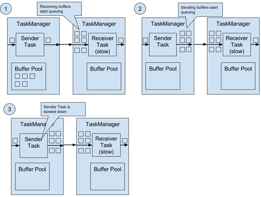
The figure shows a sender and a receiver task running on different machines.
In Chapter 2, we highlighted the importance of time semantics for stream processing applications and explained the differences between processing-time and event-time. While processing-time is easy to understand because it is based on the local time of the processing machine, it produces somewhat arbitrary, inconsistent, and non-reproducible results. In contrast, event-time semantics yield reproducible and consistent results which is a hard requirement for many stream processing use cases. However, event-time applications require some additional configuration compared to applications with processing-time semantics. Also the internals of a stream processor that supports event-time are more involved than the internals of a system that purely operates in processing-time.
Flink provides intuitive and easy-to-use primitives for common event-time processing operations but also exposes expressive APIs to implement more advanced event-time applications with custom operators. For such advanced applications, a good understanding of Flink’s internal time handling is often helpful and sometimes required. The previous chapter introduced two concepts that Flink leverages to provide event-time semantics: record timestamps and watermarks. In the following we will describe how Flink internally implements and handles timestamps and watermarks to support streaming applications with event-time semantics.
All records that are processed by a Flink event-time streaming application must have a timestamp. A timestamp associates the record with a specific point in time. Usually, the timestamp references the point in time at which the event that is encoded by the record happened. However, applications can freely choose the meaning of the timestamps as long as the timestamps of the stream records are roughly ascending as the stream is advancing. As motivated in Chapter 2, a certain degree of timestamp out-of-orderness is given in basically all real-world use cases.
When Flink processes a data stream in event-time mode, it evaluates time-based operators based on the timestamps of records. For example, a time-window operator assigns records to windows according to their associated timestamp. Flink encodes timestamps as 16-byte long values and attaches them as metadata to records. Its built-in operators interpret the long value as a Unix timestamp with millisecond precision, i.e., the number of milliseconds since 1970-01-01-00:00:00.000. However, custom operators can have their own interpretation and, for example, adjust the precision to microseconds.
In addition to record timestamps, a Flink event-time application must also provide watermarks. Watermarks are used to derive the current event-time at each task in an event-time application. Time-based operators use this time to trigger computations and make progress. For example, a time-window operator finalizes a window computation and emits the result when the operator event-time passes the window’s end boundary.
In Flink, watermarks are implemented as special records holding a timestamp long value. Watermarks flow in a stream of regular records with annotated timestamps as Figure 3-6 shows.
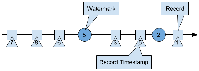
Watermarks have two basic properties.
The second property is used to handle streams with out-of-order record timestamps, such as the records with timestamps 3 and 5 in Figure 3-6. Tasks of time-based operators collect and process records with possibly unordered timestamps and finalize a computation when their event-time clock, which is advanced by received watermarks, indicates that no more records with relevant timestamps have to be expected. When a task receives a record that violates the watermark property and has smaller timestamps than a previously received watermark, it might be the case that the computation it would belong to has already been completed. Such records are called late records. Flink provides different mechanisms to deal with late records which are discussed in Chapter 6.
A very interesting property of watermarks is that they allow an application to control result completeness and latency. Watermarks that are very tight, i.e., close to the record timestamps, result in low processing latency because a task will only briefly wait for more records to arrive before finalizing a computation. At the same time, the result completeness might suffer because more records might not be included in the result and would be considered as late records. Inversely, very wide watermarks increase processing latency but improve result completeness.
In this section, we discuss how operators process watermark records. Watermarks are implemented in Flink as special records that are received and emitted by operator tasks. Tasks have an internal time service that maintains timers. A timer can be registered at the timer service to perform a computation at a specific point in time in the future. For example, a time-window task registers a timer for the ending time of each of its active windows in order to finalize a window when the event-time passed the window’s end boundary.
When a task receives a watermark, it performs the following steps.
The time service of the task identifies all timers with a time smaller than the updated event-time. The task invokes for each expired timer a call-back function that can perform a computation and emit records.
The task emits a watermark with the updated event-time.
Flink restricts the access to timestamps or watermarks through the DataStream API. Except for the ProcessFunction, functions are not able to read or modify record timestamps or watermarks. The ProcessFunction can read the timestamp of a currently processed record, request the current event-time of the operator, and register timers4. None of the functions exposes an API to set the timestamps of emitted records, manipulate the event-time clock of a task, or emit watermarks. Instead, time-based DataStream operator tasks internally set the timestamps of emitted records to ensure that they are properly aligned with the emitted watermarks. For instance, a time-window operator task attaches the end time of a window as timestamp to all records emitted by the window computation before it emits the watermark with the timestamp that triggered the computation of the window.
We explained before that a task emits watermarks and updates its event-time clock when it receives a new watermark. How this is actually done deserves a detailed discussion. As discussed in Chapter 2, Flink processes a data stream in parallel by partitioning the stream and processing each partition by a separate operator task. A partition is a stream of timestamped records and watermarks. Depending on how an operator is connected with its predecessor or successor operators, the tasks of the operator can receive records and watermarks from one or more input partitions and emit records and watermarks to one or more output partitions. In the following we describe in detail how a task emits watermarks to multiple output tasks and how it computes its event-time clock from the watermarks it received from its input tasks.
A task maintains for each input partition a partition watermark. When it receives a watermark from a partition, it updates the respective partition watermark to be the maximum of the received watermark and the current partition watermark. Subsequently the task updates its event-time clock to be the minimum of all partition watermarks. If the event-time clock advances, the task processes all triggered timers and finally broadcasts its new event-time to all downstream tasks by emitting a corresponding watermark to all connected output partitions.
Figure 3-7 visualizes how a task with four input partitions and three output partitions receives watermarks, updates its partition watermarks and event-time clock, and emits watermarks.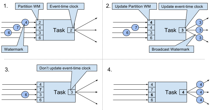
The tasks of operators with two or more input streams such as Union or CoFlatMap operators (see Chapter 5) also compute their event-time clock as the minimum of all partition watermarks, i.e., they do not distinguish between partition watermarks of different input streams. Consequently, records of both inputs are processed based on the same event-time clock.
The watermark handling and propagation algorithm of Flink ensures that operator tasks emit properly aligned timestamped records and watermarks. However, it relies on the fact that all partitions continuously provide increasing watermarks. As soon as one partition does not advance its watermarks or becomes completely idle and does not ship any records or watermarks, the event-time clock of a task will not advance and the timers of the task will not trigger. This situation is problematic for time-based operators that rely on an advancing clock to perform computations and clean up their state. Consequently, the processing latencies and state size of time-based operators can significantly increase if a task does not receive new watermarks from all input tasks in regular intervals.
A similar effect appears for operators with two input streams whose watermarks significantly diverge. The event-time clocks of a task with two input streams will correspond to the watermarks of the slower stream and usually the records or intermediate results of the faster stream are buffered in state before the event-time clock allows to process them.
So far we have explained what timestamps and watermarks are and how they are internally handled by Flink. However, we have not discussed yet where they originate from. Timestamps and watermarks are usually assigned and generated when a stream is ingested by a streaming application. Because the choice of the timestamp is application-specific and the watermarks depend on the timestamps and characteristics of the stream, applications have to explicitly assign timestamps and generate watermarks. A Flink DataStream application can assign timestamps and generate watermarks to a stream in three ways.
AssignerWithPeriodicWatermarks that extracts a timestamp from each record and is periodically queried for the current watermark. The extracted timestamps are assigned to the respective record and the queried watermarks are ingested into the stream. This function will be discussed in Chapter 6.AssignerWithPeriodicWatermarks function, this function can, but does not need to, extract a watermark from each record. The function is called AssignerWithPunctuatedWatermarks and can be used to generate watermarks that are encoded in the input records. This function will be discussed in Chapter 6 as well.User-defined timestamp assignment functions to are usually applied as closed to a source operator as possible because it is usually easier to reason about the out-of-orderness of timestamps before the stream was processed by a operator. This is also the reason why it is often not a good idea to override existing timestamps and watermarks in the middle of a streaming applications, although this is possible with the user-defined functions.
In Chapter 2 we pointed out that most streaming applications are stateful. Many operators continuously read and update some kind of state such as records collected in a window, reading positions of an input source, or custom, application-specific operator state like machine learning models. Flink treats all state - regardless of built-in or user-defined operators - the same. In this section we discuss the different types of state that Flink supports. We explain how state is stored and maintained by state backends and how stateful applications can be scaled by redistributing state.
In general, all data which are maintained by task and which are used to compute the results of the function belong to the state of the task. You can think of state as any local or instance variable that is accessed by a task’s business logic. Figure 3-8 visualizes the interaction of a task and its state.
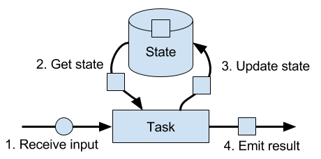
A task receives some input data. While processing the data, the task can read and update its state and compute its result based on its input data and state. A simple example is a task that continuously counts how many records it receives. When the task receives a new record, it accesses the state to get the current count, increments the count, updates the state, and emits the new count.
The application logic to read from and write to state is often straightforward. However, efficient and reliable management of state is more challenging. This includes handling of very large state, possibly exceeding memory, and ensuring that no state is lost in case of failures. All issues related to state consistency, failure handling, and efficient storage and retrieval are the responsibility and taken care of by Flink such that developers can focus on the logic of their applications.
In Flink, state is always associated with a specific operator. In order to make Flink’s runtime aware of the state of an operator, the operator needs to register its state. There are two types of state, Operator State and Keyed State, that are accessible from different scopes and which are discussed in the following sections.
Operator state is scoped to an operator task. This means that all records which are processed by the same parallel task have access to the same state. Operator state cannot be accessed by another task of the same or a different operator. Figure 3-9 visualizes how tasks access operator state.
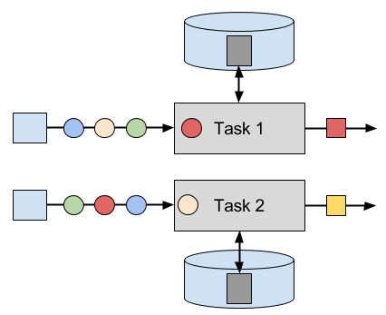
Flink offers three primitives for operator state.
Union List State represents state as a list of entries as well. It differs from regular list state in how it is restored in case of a failure or if an application is started from a savepoint. We discussed this difference later in this section.
Broadcast State is designed for the special case where the state of each task of an operator is identical. This property can be leveraged during checkpoints and when rescaling an operator. Both aspects are discussed in later sections of this chapter.
Keyed state is scoped to a key that is defined on the records of an operator’s input stream. Flink maintains one state instance per key value and partitions all records with the same key to the operator task that maintains the state for this key. When a task processes a record, it automatically scopes the state access to the key of the current record. Consequently, all records with the same key access the same state. Figure 3-10 shows how tasks interact with keyed state.
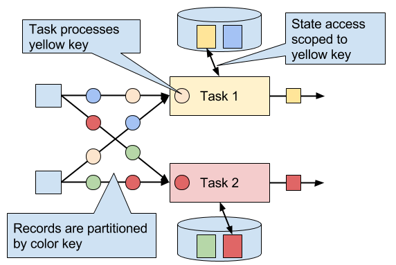
You can think of keyed state as a key-value map that is partitioned (or sharded) on the key across all parallel tasks of an operator. Flink provides a different primitives for keyed state that determine the type of the value that is stored for each key in this distribute map. We will briefly discuss the most common keyed state primitives.
State primitives expose the structure of the state to Flink and enable more efficient state accesses.
A task of a stateful operator commonly reads and updates its state for each incoming record. Because efficient state access is crucial to process records with low latency, each parallel task locally maintains its state to ensure local state accesses. How exactly the state is stored, accessed, and maintained is determined by a pluggable component that is called state backend. A state backend is responsible for mainly two aspects, local state management and checkpointing state to a remote location.
For local state management, a state backend ensures that keyed state is correctly scoped to the current key and stores and accesses all keyed state. Flink provides state backends that manage keyed state as objects stored in in-memory data structures on the JVM heap. Another state backend serializes state objects and puts them into RocksDB which writes them local hard disks. While the first option gives very fast state accesses, it is bound to the size of the memory. Accessing state stored by the RocksDB state backend is slower but its state may grow very large.
State checkpointing is important because Flink is a distributed system and state is only locally maintained. A TaskManager process (and with it all tasks running on it) may fail at any point in time such that its storage must be considered as volatile. A state backends takes care of checkpointing the state of a task to a remote and persistent storage. The remote storage for checkpointing can be a distributed file system or a database system. State backends differ in how the state is checkpointed. For instance the RocksDB state backend supports asynchronous and incremental checkpoints which significantly reduces the checkpointing overhead for very large state sizes.
We will discuss the different state backends and their pros and cons in more detail in Chapter 8.
A common requirement for streaming applications is to adjust the parallelism of operators due to increasing or decreasing input rates. While scaling stateless operators is trivial, changing the parallelism of stateful operators is much more challenging because their state needs to be re-partitioned and assigned to more or fewer parallel tasks. Flink supports four patterns to scale different types of state.
Operators with keyed state are scaled by re-partitioning keys to fewer or more tasks. However, to improve the efficiency of the necessary state transfer between tasks, Flink does not re-distributed individual keys. Instead, Flink organizes keys in so-called Key Groups. A key group is a partition of keys and Flink’s unit to assign keys to tasks. Figure 3-11 visualizes how keyed state is repartitioned in key groups.
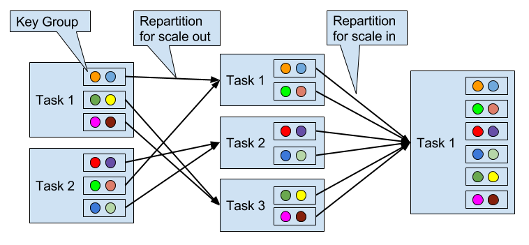
Operators with operator list state are scaled by redistributing the list entries. Conceptually, the list entries of all parallel operator tasks are collected and evenly re-distributed to a smaller or larger number of tasks. If there are fewer list entries than the new parallelism of an operator, some tasks will not receive state and have to rebuilt it from scratch. Figure 3-12 shows the redistribution of operator list state.
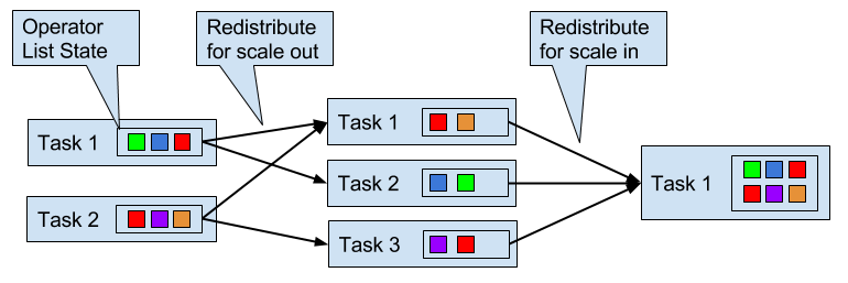
Operators with operator union list state are scaled by broadcasting the full list of state entries to each task. The task can then choose which entries to use and which to discard. Figure 3-13 shows how operator union list state is redistributed.
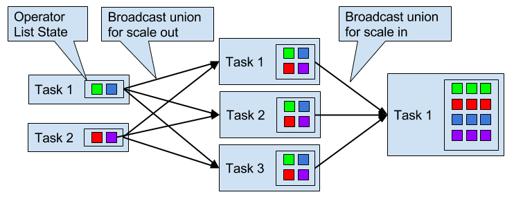
Operators with operator broadcast state are scaled up by copying the state to new tasks. This works because broadcasting state ensures that all tasks have the same state. In case of down scaling, the surplus tasks are simply canceled since state is already replicated and will not be lost. Figure 3-14 visualizes the redistribution of operator broadcast state.
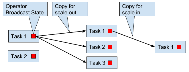
Flink is a distributed data processing system and has as such to deal with failures such as killed processes, failing machines, and interrupted network connections. Since tasks maintain their state locally, Flink has to ensure that this state does not get lost and remains consistent in case of a failure.
In this section, we present Flink’s lightweight checkpointing and recovery mechanism to guarantee exactly-once state consistency. We also discuss Flink’s unique savepoint feature, a “swiss army knife”-like tool that addresses many challenges of operating streaming applications.
Flink’s recovery mechanism is based on consistent checkpoints of application state. A consistent checkpoint of a stateful streaming application is a copy of the state of each of its tasks at a point when all tasks have processed exactly the same input. What this means can be explained by going through the steps of a naive algorithm that takes a consistent checkpoint of an application.
Note that Flink does not implement this naive algorithm. We will present Flink’s more sophisticated checkpointing algorithm later in this section.
Figure 3-15 shows a consistent checkpoint of a simple example application.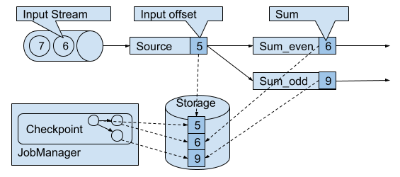
The application has a single source task that consumes a stream of increasing numbers, i.e., 1, 2, 3, and so on. The stream of numbers is partitioned into a stream of even and odd numbers. A sum operator computes with two tasks the running sums of all even and odd numbers. The source task stores the current offset of its input stream as state, the sum tasks persist the current sum value as state. In Figure 3-15, Flink took a checkpoint when the input offset was 5, and the sums were 6 and 9.
During the execution of a streaming application, Flink periodically takes consistent checkpoints of the applications state. In case of a failure, Flink uses the latest checkpoint to consistently restore the applications state and restarts the processing. Figure 3-16 visualizes the recovery process.
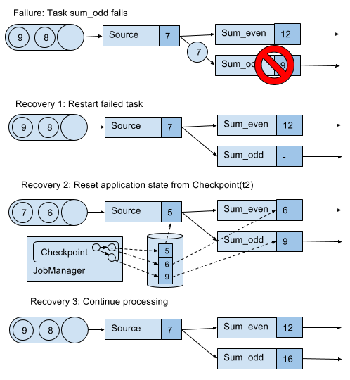
An application is recovered in three steps.
Restart all failed tasks.
Reset the state of the whole application to the latest checkpoint, i.e., resetting the state of each task.
Resume the processing of all tasks.
This checkpointing and recovery mechanism is able to provide exactly-once consistency for application state, given that all operators checkpoint and restore all of their state and that all input streams are reset to the position up to which they were consumed when the checkpoint was taken. Whether a data source can reset its input stream depends on its implementation and the external system or interface from which the stream is consumed. For instance, event logs like Apache Kafka can provide records from a previous offset of the stream. In contrast, a stream consumed from a socket cannot be reset because sockets discard data once it has been consumed. Consequently, an application can only be operated under exactly-once state consistency if all input streams are consumed by resettable data sources.
After an application is restarted from a checkpoint, its internal state is exactly the same as when the checkpoint was taken. It then starts to consume and process all data that was processed between the checkpoint and the failure. Although this means that some messages are processed twice (before and after the failure) by Flink operators, the mechanism still achieves exactly-once state consistency because the state of all operators was reset to a point that had not seen this data yet.
We also need to point out that Flink’s checkpointing and recovery mechanism only resets the internal state of a streaming application. Once the recovery completed, some records have been processed more than once. Depending on the sink operators of an applications, it might happen that some result records are emitted multiple times to downstream systems, such as an event log, a file system, or a database. For selected systems, Flink provides sink functions that feature exactly-once output for example by committing emitted records on checkpoint completion. Another approach that works for many common sink systems are idempotent updates. The challenge of end-to-end exactly-once applications and approaches to address it are discussed in detail in Chapter 7.
Flink’s recovery mechanism is based on consistent application checkpoints. The naive approach to take a checkpoint from a streaming application, i.e, to pause, checkpoint, and resume the application, suffers from its “stop-the-world” behavior which is not acceptable for applications that have even moderate latency requirements. Instead, Flink implements an algorithm which is based on the well-known Chandy-Lamport algorithm for distributed snapshots. The algorithm does not pause the complete application but decouples the checkpointing of individual tasks such that some tasks continue processing while others persist their state.In the following we explain how this algorithm works.
Flink’s checkpointing algorithm is based on a special type of record that is called checkpoint barrier. Similar to watermarks, checkpoint barriers are injected by source operators into the regular stream of records and cannot overtake or be passed by any other record. A checkpoint barrier carries a checkpoint ID to identify the checkpoint it belongs to and logically splits a stream into two parts. All state modifications due to records that precede a barrier are included in the checkpoint and all modifications due to records that follow the barrier are included in a later checkpoint.
We use an example of a simple streaming application to explain the algorithm step-by-step. The application consists of two source tasks which consume a stream of increasing numbers. The output of the source tasks is partitioned into streams of even and odd numbers. Each partition is processed by a task that computes the sum of all received number and forwards the updated sum to a sink. The application is depicted in Figure 3-17.
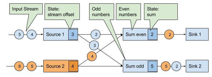
A checkpoint is initiated by the JobManager by sending a message with a new checkpoint ID to each data source task as shown in Figure 3-18.
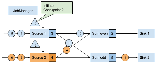
When a data source task receives the message, it pauses emitting records, triggers a checkpoint of its local state at the state backend, and broadcasts checkpoint barriers with the checkpoint ID via all outgoing stream partitions. The state backend notifies the task once the task checkpoint is complete and the task acknowledges the checkpoint at the JobManager. After all barriers are sent out, the source continues its regular operations. By injecting the barrier into its output stream, the source function defines the stream position on which the checkpoint is taken. Figure 3-19 shows the streaming application after both source tasks checkpointed their local state and emitted checkpoint barriers.
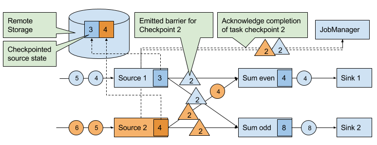
The checkpoint barriers emitted by the source tasks are shipped to the subsequent tasks. Similar to watermarks, checkpoint barriers are broadcasted to all connected parallel tasks. Checkpoint barriers must be broadcasted to ensure that each task receives a checkpoint from each of its input streams, i.e., all downstream connected tasks. When a task receives a barrier for a new checkpoint, it waits for the arrival of all barriers for the checkpoint. While it is waiting, it continues processing records from stream partitions that did not provided a barrier yet. Records which arrive via partitions that forwarded a barrier already must not be processed and need to be buffered. The process of waiting for all barriers to arrive is called barrier alignment and depicted in Figure 3-20.
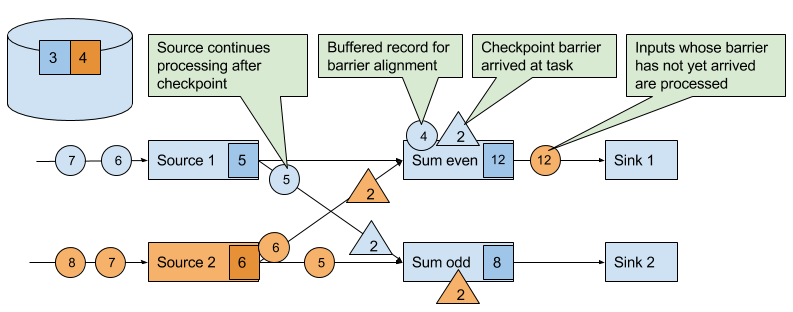
As soon as all barriers have arrived, the task initiates a checkpoint at the state backend and broadcasts the checkpoint barrier to all of its downstream connected tasks as shown in Figure 3-21.
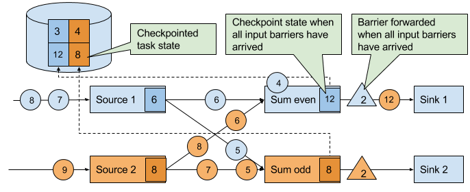
Once all checkpoint barriers have been emitted, the task starts to process the buffered records. After all buffered records have been emitted, the task continues processing its input streams. Figure 3-22 shows the application at this point.
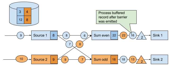
Eventually, the checkpoint barriers arrive at a sink task. When a sink task receives a barrier, it performs a barrier alignment, checkpoints its own state, and acknowledges the reception of the barrier to the JobManager. The JobManager records the checkpoint of an application as completed once it received a checkpoint acknowledgement from all tasks of the application. Figure 3-23 shows the final step of the checkpointing algorithm. The completed checkpoint can be used to recover the application from a failure as described before.
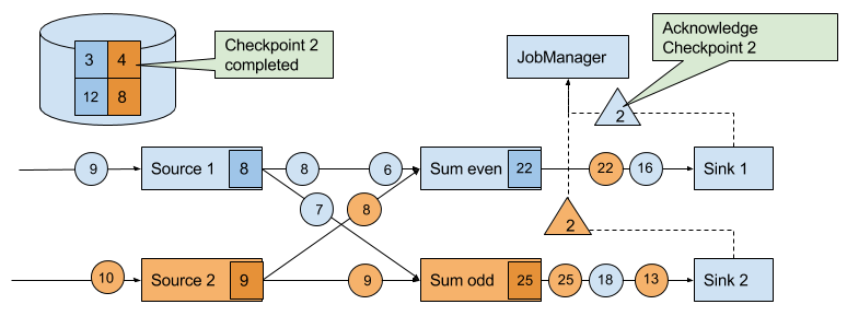
The discussed algorithm produces consistent distributed checkpoints from streaming applications without stopping the whole application. However, it has two properties that can increase the latency of an application. Flink’s implementation features tweaks that improve the performance of the application under certain conditions.
The first spot is the process of checkpointing the state of a task. During this step, a task is blocked and its input is buffered. Since operator state can become quite large and checkpointing means sending the data over the network to a remote storage system, taking a checkpoint can easily take several seconds, much too long for latency sensitive applications. In Flink’s design it is the responsibility of the state backend to perform a checkpoint. How exactly the state of a task is copied depends on the implementation of the state backend and can be optimized. For example, the RocksDB state backend supports asynchronous and incremental checkpoints. When a checkpoint is triggered, the RocksDB state backend, locally snapshots all state modifications since the last checkpoint (a very lightweight and fast operation due to RocksDBs design) and immediately returns such that the task can continue processing. A background thread asynchronously copies the local snapshot to the remote storage and notifies the task once it completed the checkpoint. Asynchronous checkpointing significantly reduces the latency of copying state to remote storage. Incremental checkpointing reduces the amount of data to transfer.
Another reason for increased latency can result from the record buffering during the barrier alignment step. For applications that require consistently very low latency and can tolerate at-least-once state guarantees, Flink can be configured to process all arriving records during buffer alignment instead of buffering those for which the barrier has already arrived. Once all barriers for a checkpoint have arrived, the operator checkpoints the state, which might now also include modifications cause by records that would usually belong to the next checkpoint. In case of a failure, these records will be processed again which means that the checkpoint provides at-least-once instead of exactly-once consistency guarantees.
Flink’s recovery algorithm is based on state checkpoints. Checkpoints are periodically taken and automatically discarded when a new checkpoint completes. Their sole purpose is to ensure that in case of a failure an application can be restarted without losing state. However, consistent snapshots of the state of an application can be used for many more purposes.
One of Flink’s most valuable and unique features are savepoints. In principle, savepoints are checkpoints with some additional metadata and are created using the same algorithm as checkpoints. Flink does not automatically take a savepoint, but a user (or external scheduler) has to trigger its creation. Flink does also not automatically clean up savepoints.
Given an application and a compatible savepoint, you can start the application from the savepoint which will initialize state of the application to the state of the savepoint and run the application from the point at which the savepoint was taken. While this sounds basically the same as recovering an application from a failure using a checkpoint, failure recovery is actually just a special case because it starts the same application with the same configuration on the same cluster. Starting an application from a savepoint allows you to do much more.
Since savepoints are such a powerful feature, many users periodically take savepoints to be able to go back in time. One of the most interesting applications of savepoints we have seen in the wild is to migrate streaming applications to the data center that provides the lowest instance prices.
In this chapter we have discussed Flink’s high-level architecture and the internals of its networking stack, event-time processing mode, state management, and failure recovery mechanism. You will find knowledge about these internals helpful when designing advanced streaming applications, setting up and configuring clusters, and operating streaming applications as well as reasoning about their performance.
1 Chapter 10 will discuss how the DataStream API allows to control the assignment and grouping of tasks.
2 Batch applications can - in addition to pipelined communication - exchange data by collecting outgoing data at the sender. Once the sender task completes, the data is sent as a batch over a temporary TCP connection to the receiver
3 A TaskManager ensures that each task has at least one incoming and one outgoing buffer and respects additional buffer assignment constraints to avoid deadlocks and maintain smooth communication.
4 The ProcessFunction is discussed in more detail in Chapter 6.
Time to get our hands dirty and start developing Flink applications! In this chapter, you will learn how to setup an environment to develop, run, and debug Flink applications.
We will start discussing required software and explain how to obtain the code examples of this book. Using these examples, we will show how Flink applications are executed and debugged in an IDE. Finally, we show how to bootstrap a Flink Maven project that serves as a starting point for a new application.
First, let’s discuss the software that is required to develop Flink applications. You can develop and execute Flink applications on Linux, macOS, and Windows. However, UNIX-based setups enjoy the richest tooling support because this environment is preferred by most Flink developers. We will be assuming a UNIX-based setup in the rest of this chapter. As a Windows user you can use Windows subsystem for Linux (WSL), Cygwin, or a Linux virtual machine to run Flink in a UNIX environment.
Flink’s DataStream API is available for Java and Scala. Hence, a Java JDK is required to implement Flink DataStream applications:
We assume that the following software is installed as well, although it is not strictly required to develop Flink applications:
Even though Flink is a distributed data processing system, you will typically develop and run initial tests on your local machine. This makes development easier and simplifies cluster deployment, as you can run the exact same code in a cluster environment without making any changes. In the following, we describe how to obtain the code examples of the book, how to import them into IntelliJ, how to run an example application, and how to debug it.
The code examples of this book are hosted on GitHub. At https://github.com/streaming-with-flink, you will find one repository with Scala examples and one repository with Java examples. We will be using the Scala repository for the setup, but you should be able to follow the same instructions if you prefer Java.
Open a terminal and run the following Git command to clone the examples repository to your local machine.
> git clone https://github.com/streaming-with-flink/examples-scala
You can also download the source code of the examples as a zip-archive from Github.
> wget https://github.com/streaming-with-flink/examples-scala/archive/master.zip
> unzip master.zip
The book examples are provided as a Maven project. You will find the source code in the src/ directory, grouped by chapter:
.
└── main
    └── scala
        └── io
            └── github
                └── streamingwithflink
                    ├── chapter1
                    │   └── AverageSensorReadings.scala
                    ├── chapter4
                    │   └── ...
                    ├── chapter5
                    │   └── ...
                    ├── ...
                    │   └── ...
                    └── util
                        ├── SensorReading.scala
                        ├── SensorSource.scala
                        └── SensorTimeAssigner.scala
Now open your IDE and import the Maven project. The import steps are similar for most IDEs. In the following, we explain this step in detail for IntelliJ.
Select Import Project. Find the book examples folder and hit Open -> Import project from external model -> Maven and click Next. Select the project to import (there should be only one) and set up your SDK, give your project a name, and click Finish:
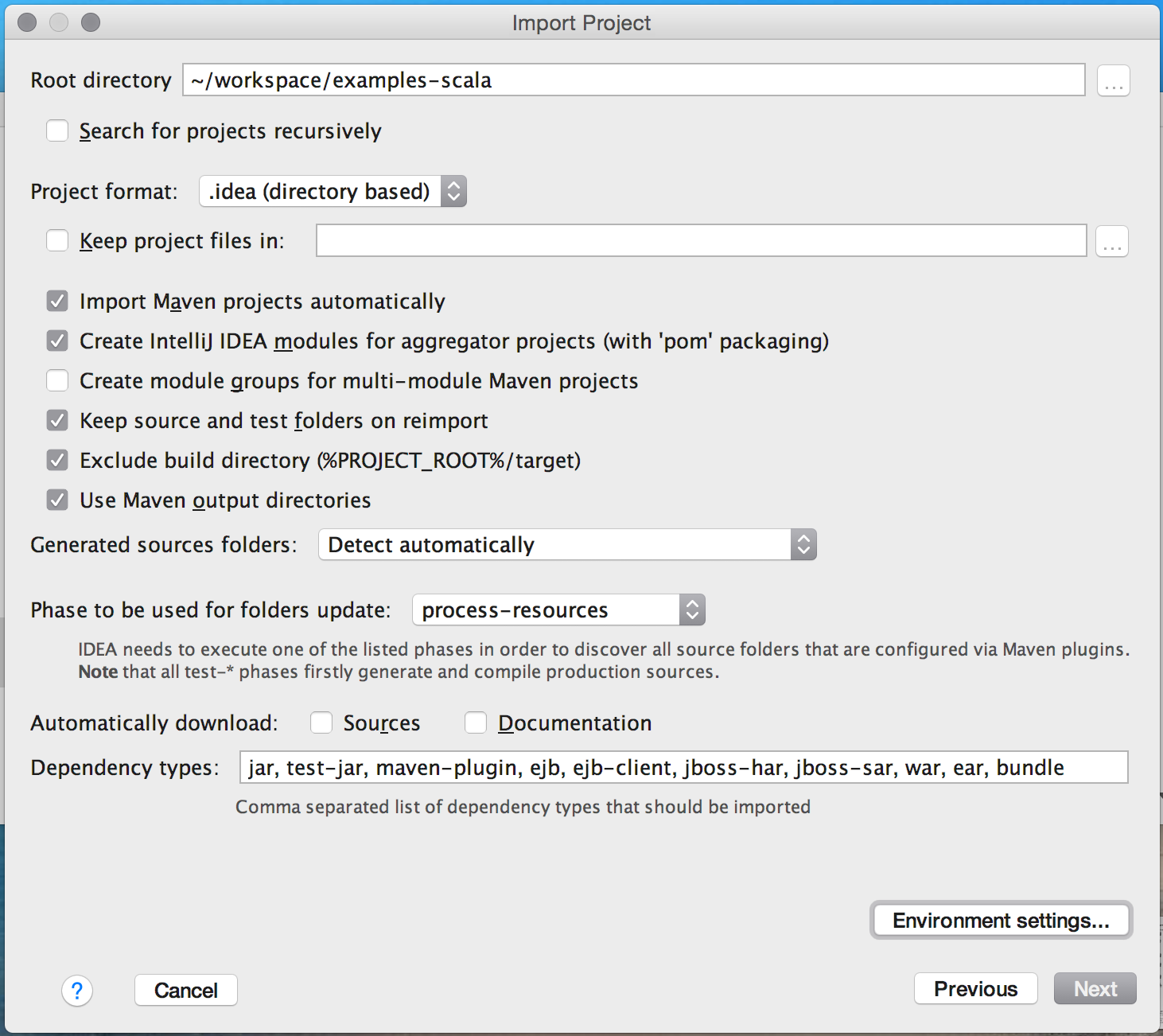
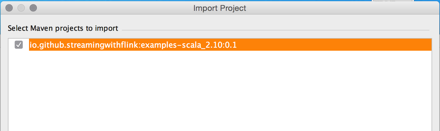
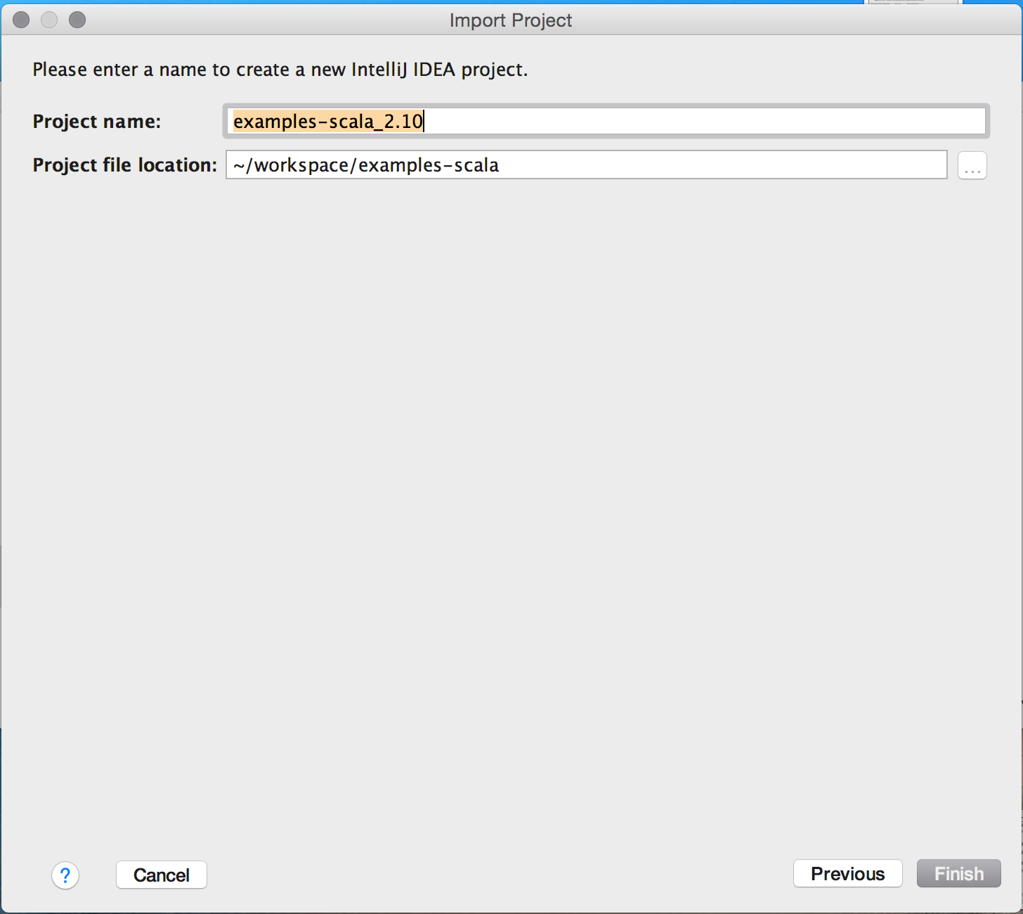
That’s it! You should now be able to browse and inspect the code of the book examples.
Next, let’s run one of the book example applications in your IDE. Search for the AverageSensorReadings class and open it. As discussed in Chapter 1, the program generates read events for multiple thermal sensors, converts the temperature of the events from Fahrenheit to Celsius, and computes the average temperature of each sensor every second. The results of the program are emitted to standard-out. Just like many DataStream applications, the source, sink, and operators of the program are assembled in the main() method of the AverageSensorReadings class.
To start the the application, run the main() method. The output of the program is written to the standard-out (or console) window of your IDE. The output starts with a few log statements about the states that parallel operator tasks go through, such as SCHEDULING, DEPLOYING, and RUNNING. Once all tasks are up and running, the program starts to produce its results that should look similar to the following lines:
2> SensorReading(sensor_31,1515014051000,23.924656183848732)
4> SensorReading(sensor_32,1515014051000,4.118569049862492)
1> SensorReading(sensor_38,1515014051000,14.781835420242471)
3> SensorReading(sensor_34,1515014051000,23.871433252250583)
The program will continue to generate new events, process them, and emit new results every second until you terminate it.
Now let’s quickly discuss what is happening under the hood. As explained in Chapter 3, a Flink application is submitted to the JobManager (master) which distributes execution tasks to one or more TaskManagers (workers). Since Flink is a distributed system, the JobManager and TaskManagers typically run as separate JVM processes on different machines. Usually, the program’s main() method assembles the dataflow and submits it to a remote JobManager when the StreamExecutionEnvironment.execute() method is called.
However, there is also a mode in which the call of the execute() method starts a JobManager and a TaskManager (by default with as many slots as available CPU threads) as separate threads within the same JVM. Consequently, the whole Flink application is multi-threaded and executed within the same JVM process. This mode is used to execute a Flink program within an IDE.
Due to the single JVM execution mode, it is also possible to debug Flink applications in an IDE almost like any other program in your IDE. You can define breakpoints in the code and debug your application as you would normally do.
However, there are a few aspects to consider when debugging a Flink application in an IDE:
Importing the book examples repository into your IDE to experiment with Flink is a good first step. However, you should also know how to create a new Flink project from scratch.
Flink provides Maven archetypes to generate Maven projects for Java or Scala Flink applications. Open a terminal and run the following command to create a Flink Maven Quickstart Scala project as a starting point for your Flink application:
mvn archetype:generate                            \
   -DarchetypeGroupId=org.apache.flink            \
   -DarchetypeArtifactId=flink-quickstart-scala   \
   -DarchetypeVersion=1.5.2                       \
   -DgroupId=org.apache.flink.quickstart          \
   -DartifactId=flink-scala-project               \
   -Dversion=0.1                                  \
   -Dpackage=org.apache.flink.quickstart          \
   -DinteractiveMode=false
This will generate a Maven project for Flink 1.5.2 in a folder called flink-scala-project. You can change the Flink version, group and artifact IDs, version, and generated package by changing the respective parameters of the above mvn command. The generated folder contains a src/ folder and a pom.xml file. The src/ folder has the following structure:
src/
└── main
    ├── resources
    │   └── log4j.properties
    └── scala
        └── org
            └── apache
                └── flink
                    └── quickstart
                        ├── BatchJob.scala
                        ├── SocketTextStreamWordCount.scala
                        ├── StreamingJob.scala
                        └── WordCount.scala
The project contains two example applications and two skeleton files which you can use as templates for your own programs or simply delete. WordCount.scala contains an implementation of the popular WordCount example using Flink’s DataSet API. SocketStreamWordCount.scala uses the DataStream API to implement a streaming WordCount program that reads words from a text socket. BatchJob.scala and StreamingJob.scala provide skeleton code for a batch and a streaming Flink program respectively.
You can import the project in your IDE following the steps we described in the previous section or you can execute the following command to build a jar:
mvn clean package -Pbuild-jar
If the command is completed successfully, you will find a new target folder in your project folder which contains a jar file called flink-scala-project-0.1.jar. The generated pom.xml file also contains instructions on how to add new dependencies to your project.
This chapter introduces the basics of Flink’s DataStream API. We show the structure and components of a typical Flink streaming application, we discuss Flink’s type systems and the supported data types, and we present data and partitioning transformations. Window operators, time-based transformations, stateful operators, and connectors are discussed in the next chapters. After reading this chapter, you will have learned how to implement a stream processing application with basic functionality. We use Scala for the code examples, but the Java API is mostly analogous (exceptions or special cases will be pointed out).
Let’s start with a simple example to get a first impression of what it is like to write streaming applications with the DataStream API. We will use this example to showcase the basic structure of a Flink program and introduce some important features of the DataStream API. Our example application ingests a stream of temperature measurements from multiple sensors.
First, let’s have a look at the data type we will be using to represent sensor readings:
caseclassSensorReading(id:String,timestamp:Long,temperature:Double)
The following program converts the temperatures from Fahrenheit degrees to Celsius degrees and computes the average temperature every five seconds for each sensor.
// Scala object that defines the DataStream program in the// main() method.objectAverageSensorReadings{// main() defines and executes the DataStream programdefmain(args:Array[String]){// set up the streaming execution environmentvalenv=StreamExecutionEnvironment.getExecutionEnvironment// use event time for the applicationenv.setStreamTimeCharacteristic(TimeCharacteristic.EventTime)// create a DataStream[SensorReading] from a stream sourcevalsensorData:DataStream[SensorReading]=env// ingest sensor readings with a SensorSource SourceFunction.addSource(newSensorSource).setParallelism(4)// assign timestamps and watermarks (required for event time).assignTimestampsAndWatermarks(newSensorTimeAssigner)valavgTemp:DataStream[SensorReading]=sensorData// convert Fahrenheit to Celsius with an inline// lambda function.map(r=>{valcelsius=(r.temperature-32)*(5.0/9.0)SensorReading(r.id,r.timestamp,celsius)})// organize readings by sensor id.keyBy(_.id)// group readings in 5 second tumbling windows.timeWindow(Time.seconds(5))// compute average temperature using a user-defined function.apply(newTemperatureAverager)// print result stream to standard outavgTemp.()// execute applicationenv.execute("Compute average sensor temperature")}}
You have probably already noticed that Flink programs are defined and submitted for execution in regular Scala or Java methods. Most commonly, this is done in a static main method. In our example, we define the AverageSensorReadings object and include most of the application logic inside main().
The structure of a typical Flink streaming application consists of the following parts:
We now look into these parts in detail using the above example.
The first thing a Flink application needs to do is set up its execution environment. The execution environment determines whether the program is running on a local machine or on a cluster. In the DataStream API, the execution environment of an application is represented by the StreamExecutionEnvironment. In our example, we retrieve the execution environment by calling the getExecutionEnvironment(). This method returns a local or remote environment, depending on the context in which the method is invoked. If the method is invoked from a submission client with a connection to a remote cluster, a remote execution environment is returned. Otherwise, it returns a local environment.
It is also possible to explicitly create local or remote execution environments as follows:
// create a local stream execution environmentvallocalEnv:StreamExecutionEnvironment.createLocalEnvironment()// create a remote stream execution environmentvalremoteEnv=StreamExecutionEnvironment.createRemoteEnvironment("host",// hostname of JobManager1234,// port of JobManager process"path/to/jarFile.jar)// JAR file to ship to the JobManager
The JAR file that is shipped to the JobManager must contain all resources that are required to execute the streaming application.
Next, we use env.setStreamTimeCharacteristic(TimeCharacteristic.EventTime) to instruct our program to interpret time semantics using event time. The execution environment allows for more configuration options, such as setting the program parallelism and enabling fault tolerance.
Once the execution environment has been configured, it is time to do some actual work and start processing streams. The StreamExecutionEnvironment provides methods to create a stream source that ingests data streams into the application. Data streams can be ingested from sources such as message queues, files, or also be generated on the fly.
In our example, we use
val sensorData: DataStream[SensorReading] =
  env.addSource(new SensorSource)
to connect to the source of the sensor measurements and create an initial DataStream of type SensorReading. Flink supports many data types which we describe in the next section. Here, we use a Scala case class as the data type that we defined before. A SensorReading contains the sensor id, a timestamp denoting when the measurement was taken, and the measured temperature. The following two methods configure the input data source to be executed with a parallelism of 4 by calling setParallelism(4) and assign timestamps and watermarks, which are required for event time using assignTimestampsAndWatermarks(new SensorTimeAssigner). The implementation details of SensorTimeAssigner should not concern us for the moment.
Once we have a DataStream, we can apply a transformation on it. There are different types of transformations. Some transformations can produce a new DataStream, possibly of a different type, while other transformations do not modify the records of the DataStream but reorganize it by partitioning or grouping. The logic of an application is defined by chaining transformations.
In our example, we first apply a map() transformation, which converts the temperature of each sensor reading to celsius. Then, we use the keyBy() transformation to partition the sensor readings by their sensor id. Subsequently, we define a timeWindow() transformation, which groups the sensor readings of each sensor id partition into tumbling windows of 5 seconds. Window transformations are described in detail in the next chapter. Finally, we apply a user-defined function (UDF) that computes the average temperature on each window. We discuss more about defining UDFs in the DataStream API later in this chapter.
Streaming applications usually emit their result to some external system, such as Apache Kafka, a file system, or a database. Flink provides a well maintained collection of stream sinks that can be used to write data to different systems. It is also possible to implement own streaming sinks. There are also applications that do not emit results but keep them internally to serve them via Flink’s queryable state feature.
In our example, the result is a DataStream[SensorReading] with the average measured temperature over 5 seconds of each sensor. The result stream is written to the standard output by calling print().
Please note that the choice of a streaming sink affects the end-to-end consistency of an application, i.e., whether the result of the application is provided with at-least once or exactly-once semantics. The end-to-end consistency of the application depends on the integration of the chosen stream sinks with Flink’s checkpointing algorithm. We will discuss this topic in more detail in Chapter 7.
When the application has been completely defined, it can be executed by calling StreamExecutionEnvironment.execute(). Flink programs are lazy executed. That is, that all methods to create stream sources and transformation have not resulted in any data processing so far. Instead, the execution environment constructs an execution plan which starts from all stream sources created from the environment and includes all transformations which are transitively applied to these sources.
Only when execute() is called, the system triggers the execution of the constructed plan. Depending on the type of execution environment, an application is locally executed or sent to a remote JobManager for execution.
In Flink, type information is required to properly choose serializers, deserializers, and comparators, to efficiently execute functions, and to correctly manage state. For instance, records of a DataStream need to be serialized in order to transfer them over the network or write them to a storage system, for example during checkpointing. The more the system knows about the types of the data it processes the better optimization it can perform.
Flink supports the many common data types that you are used to working with already. The most widely used types can be grouped into the following categories:
Types that are not especially handled are treated as generic types and serialized using the Kryo serialization framework.
Let us look into each type category by example.
All Java and Scala primitive types, such as Int (or Integer for Java), String, and Double, are supported as DataStream types. Here is an example that processes a stream of Long values and increments each element:
valnumbers:DataStream[Long]=env.fromElements(1L,2L,3L,4L)numbers.map(n=>n+1)
Tuples are composite data types that consist of a fixed number of typed fields.
The Scala DataStream API uses regular Scala tuples. Below is an example that filters a DataStream of tuples with two fields. We will discuss the semantics of the filter transformation in the next section:
// DataStream of Tuple2[String, Integer] for Person(name, age)valpersons:DataStream[(String,Integer)]=env.fromElements(("Adam",17),("Sarah",23))// filter for persons of age > 18persons.filter(p=>p._2>18)
Flink provides efficient implementations of Java tuples. Flink’s Java tuples can have up to 25 fields and each length is implemented as a separate class, i.e., Tuple1, Tuple2, up to, Tuple25. The tuple classes are strongly typed.
We can rewrite the filtering example in the Java DataStream API as follows:
// DataStream of Tuple2<String, Integer> for Person(name, age)DataStream<Tuple2<String,Integer>>persons=env.fromElements(Tuple2.of("Adam",17),Tuple2.of("Sarah",23));// filter for persons of age > 18persons.filter(newFilterFunction<Tuple2<String,Integer>(){@Overridepublicbooleanfilter(Tuple2<String,Integer>p)throwsException{returnp.f1>18;}})
Tuple fields can be accessed by the name of their public fields f0, f1, f2, etc. as above or by position using the Object getField(int pos) method, where indexes start at 0:
Tuple2<String,Integer>personTuple=Tuple2.of("Alex","42");Integerage=personTuple.getField(1);// age = 42
In contrast to their Scala counterparts, Flink’s Java tuples are mutable, such that the values of fields can be reassigned. Hence, functions can reuse Java tuples in order to reduce the pressure on the garbage collector.
personTuple.f1=42;// set the 2nd field to 42personTuple.setField(43,1);// set the 2nd field to 43
Flink supports Scala case classes; classes that can be decomposed by pattern matching. Case class fields are accessed by name. In the following example, we define a case class Person with two fields, name and age. Similar as for the tuples, we filter the DataStream by age.
caseclassPerson(name:String,age:Int)valpersons:DataStream[Person]=env.fromElements(Person("Adam",17),Person("Sarah",23))// filter for persons with age > 18persons.filter(p=>p.age>18)
Flink analyzes each type that does not fall into any category and checks if it can be identified and handled as a POJO type. Flink accepts a class as POJO if it satisfies the following conditions:
Y getX() and setX(Y x) for a field x of type Y.For example, the following Java class will be identified as a POJO by Flink:
publicclassPerson{// both fields are publicpublicStringname;publicintage;// default constructor is presentpublicPerson(){}publicPerson(Stringname,intage){this.name=name;this.age=age;}}DataStream<Person>persons=env.fromElements(newPerson("Alex",42),newPerson("Wendy",23));
Avro generated classes are automatically identified by Flink and handled as POJOs.
Value types implement the org.apache.flink.types.Value interface. The interface consists of two methods read() and write() to implement serialization and deserialization logic. For example, the methods can be leveraged to encode common values more efficiently than general-purpose serializers.
Flink comes with a few built-in Value types, such as IntValue, DoubleValue, and StringValue, that provide mutable alternatives for Java’s and Scala’s immutable primitive types.
Flink supports several special-purpose types, such as Scala’s Either, Option, and Try types, and Flink’s Java version of the Either type. Similarly to Scala’s Either, it represents a value of one of two possible types, Left or Right. In addition, Flink supports primitive and object Array types, Java Enum types and Hadoop Writable types.
In many cases, Flink is able to automatically infer types and choose the appropriate serializers and comparators. Sometimes, though, this is not a straightforward task. For example, Java erases generic type information. Flink tries to reconstruct as much type information as possible via reflection, using function signatures and subclass information. Type inference is as well possible when the return type of a function depends on its input type. If a function uses generic type variables in the return type that cannot be inferred from the input type, you can give Flink hints about your types using the returns() method.
You can provide type hints with a class, as in the following example:
DataStream<MyType> result = input
   .map(new MyMapFunction<Long, MyType>())
   .returns(MyType.class);
If the function uses generic type variables in the return type that cannot be inferred from the input type, you need to provide a TypeHint instead:
DataStream<Integer>result=input.flatMap(newMyFlatMapFunction<String,Integer>()).returns(newTypeHint<Integer>(){});
classMyFlatMapFunction<T,O>implementsFlatMapFunction<T,O>{publicvoidflatMap(Tvalue,Collector<O>out){...}}
The central class in Flink’s type system is TypeInformation. It provides the system with the necessary information it needs to generate serialiazers and comparators. For instance, when you join or group by some key, this is the class that allows Flink to perform the semantic check of whether the fields used as keys are valid.
You might in fact use Flink for a while without ever needing to worry about this class, as it usually does all type handling for you automatically. However, when you start writing more advanced applications, you might want to define your own types and tell Flink how to handle them efficiently. In such cases, it is helpful to be familiar with some of the class details.
TypeInformation maps fields from the types to fields in a flat schema. Basic types are mapped to single fields and tuples and case classes are mapped to as many fields as the class has. The flat schema must be valid for all type instances, thus variable length types like collections and arrays are not assigned to individual fields, but they are considered to be one field as a whole.
The following example defines a TypeInformation and a TypeSerializer for a 2-tuple:
// get the execution configvalconfig=inputStream.executionConfig...// create the type informationvaltupleInfo:TypeInformation[(String,Double)]=createTypeInformation[(String,Double)//createaserializervaltupleSerializer=typeInfo.createSerializer(config)
In the Scala API, Flink uses macros that run at compile time. To access the ‘createTypeInformation’ macro function, make sure to always add the following import statement:
import org.apache.flink.streaming.api.scala._
In this section we give an overview of the basic transformations for the DataStream API. Time-related operators, such as window operators, and further specialized transformations are described in the following chapters. Stream transformations are applied on one or more input streams and transform them into one ore more output streams. Writing a DataStream API program essentially boils down to combining such transformations to create a dataflow graph that implements the application logic.
Most stream transformations are based on user-defined functions (UDF). UDFs encapsulate the user application logic and define how the elements of the input stream(s) are transformed into the elements of the output stream. UDFs are defined as classes that extend a transformation-specific function interface, such as FilterFunction in the following example:
classMyFilterFunctionextendsFilterFunction[Int]{overridedeffilter(value:Int):Boolean={value>0;}}
The function interface defines the transformation method that needs to be implemented by the user, such as filter() in the example above.
Most function interfaces are designed as SAM (single abstract method) interfaces. Hence they can be implemented as lambda functions in Java 8. The Scala DataStream API also has built-in support for lambda functions. When presenting the transformations of the DataStream API, we show the interfaces for all function classes, but mostly use lambda functions instead of function classes in code examples for brevity.
The DataStream API provides transformations for the most common data transformation operations. If you are familiar with batch data processing APIs, functional programming languages, or SQL you will find the API concepts very easy to grasp. In the following, we present the transformations of the DataStream API in four groups:
Basic transformations process individual events. We explain their semantics and show code examples.
DataStream -> DataStream]The filter transformation drops or forwards events of a stream by evaluating a boolean condition on each input event. A return value of true preserves the input event and forwards it to the output, false results in dropping the event. A filter transformation is specified by calling the DataStream.filter() method. Figure 5.2 shows a filter operation that only preserves white squares.

The boolean condition is implemented as an UDF either using the FilterFunction interface or a lambda function. The FilterFunction interface is typed on the type of the input stream and defines the filter() method that is called with an input event and returns a boolean.
// T: the type of elements
FilterFunction[T]
    > filter(T): Boolean
The following example shows a filter that drops all sensor measurements with temperature below 25 degrees:
valreadings:DataStream[SensorReadings]=...valfilteredSensors=readings.filter(r=>r.temperature>=25)
DataStream -> DataStream]The map transformation is specified by calling the DataStream.map() method. It passes each incoming event to a user-defined mapper that returns exactly one output event, possibly of a different type. Figure 5.1 shows a map transformation that converts every square into a circle.

The mapper is typed to the types of the input and output events and can be specified using the MapFunction interface. It defines the map() method that transforms an input event into exactly one output event.
// T: the type of input elements
// O: the type of output elements
MapFunction[T, O]
    > map(T): O
Below is a simple mapper that projects the first field (id) of each ATLAS-CURSOR-SensorReading in the input stream:
valreadings:DataStream[SensorReading]=...valsensorIds:DataStream[String]=readings.map(newMyMapFunction)classMyMapFunctionextendsProjectionMap[SensorReading,String]{overridedefmap(r:SensorReading):String=r.id}
When using the Scala API or Java 8, the mapper can also be expressed as a lambda function.
valreadings:DataStream[SensorReading]=...valsensorIds:DataStream[String]=readings.map(r=>r.id)
DataStream -> DataStream]FlatMap is similar to map, but it can produce zero, one, or more output events for each incoming event. In fact, flatMap is a generalization of filter and map and it can be used to implement both those operations. Figure 5.3 shows a flatMap operation that differentiates its output based on the color of the incoming event. If the input is a white square, it outputs the event unmodified. Black squares are duplicated, and gray squares are filtered out.

The flatMap transformation applies a UDF on each incoming event. The corresponding FlatMapFunction defines the flatMap() method, which may return none, one, or more events as result by passing them to the Collector object.
// T: the type of input elements
// O: the type of output elements
FlatMapFunction[T, O]
    > flatMap(T, Collector[O]): Unit
The example below shows a flatMap transformation that transforms the stream of sensor String ids. Our simple event source for sensor readings produces sensor ids of the form “sensor_N”, where N is an integer. The flatMap function below separates each id into its prefix, “sensor_” and the sensor number and emits them both:
valsensorIds:DataStream[String]=...valsplitIds:DataStream[String]=sensorIds.flatMap(id=>id.split("_"))
Note that each word will be emitted as an individual record, that is flatMap flattens the output collection.
A common requirement of many applications is to process groups of events together that share a certain property. The DataStream API features the abstraction of a KeyedStream, which is a DataStream that has been logically partitioned into disjoint substreams of events that share the same key.
Stateful transformations that are applied on a KeyedStream read from and write to state in the context of the currently processed event’s key. This means that all events with the same key can access the same state and thereby be processed together. Please note that stateful transformations and keyed aggregates have to be used with care. If the key domain is continuously growing, for example because the key is a unique transaction ID, then the application might eventually suffer from memory problems. Please refer to Chapter 8 which discusses stateful functions in detail.
A KeyedStream can be processed using the map, flatMap, and filter transformations that you saw before. In the following you will see how to use a keyBy transformation to convert a DataStream into a KeyedStream and keyed transformations such as rolling aggregations and reduce.
DataStream -> KeyedStream]The keyBy transformation converts a DataStream into a KeyedStream using a specified key. Based on the key, it assigns events to partitions. Events with different keys can be assigned to the same partition, but it is guaranteed that elements with the same key will always be in the same partition. Hence, a partition consists of possibly multiple logical substreams, each having a unique key.
Considering the color of the input event as the key, Figure 5.4 below assigns white and gray events to one partition and black events to the other:
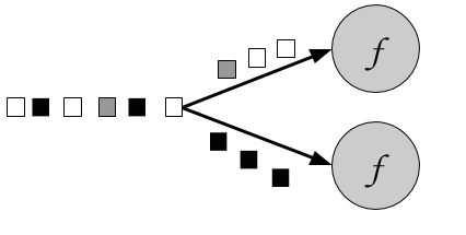
The keyBy() method receives an argument that specifies the key (or keys) to group by and returns a KeyedStream. There are different ways to specify keys. We look into them in the section “Defining Keys" later in the chapter. The following example groups the sensor readings stream by id:
valreadings:DataStream[SensorReading]=...valkeyed:KeyedStream[SensorReading,String]=readings.keyBy(_.id)
KeyedStream -> DataStream]Rolling aggregation transformations are applied on a KeyedStream and produce a stream of aggregates, such as sum, minimum, and maximum. A rolling aggregate operator keeps an aggregated value for every observed key. For each incoming event, the operator updates the corresponding aggregate value and emits an event with the updated value. A rolling aggregation does not require an user-defined function but receives an argument that specifies on which field the aggregate is computed. The DataStream API provides the following rolling aggregation methods:
sum(): a rolling sum of the input stream on the specified fieldmin(): a rolling minimum of the input stream on the specified fieldmax(): a rolling maximum of the input stream on the specified fieldminBy(): a rolling minimum of the input stream that returns the event with the lowest value observed so farmaxBy(): a rolling maximum of the input stream that returns the event with the highest value observed so farIt is not possible to combine multiple rolling aggregation methods, i.e., only a single rolling aggregate can be computed at a time.
Consider the following example:
valinputStream:DataStream[(Int,Int,Int)]=env.fromElements((1,2,2),(2,3,1),(2,2,4),(1,5,3))valresultStream:DataStream[(Int,Int,Int)]=inputStream.keyBy(0)// key on first field of the tuple.sum(1)// sum the second field of the tupleresultStream.()
In the example the tuple input stream is keyed by the first field and the rolling sum is computed on the second field. The output of the example is (1,2,2) followed by (1,7,2) for the key “1” and (2,3,1) followed by (2,5,1) for the key “2”. The first field is the common key, the second field is the sum and the third field is not defined.
KeyedStream -> DataStream]The reduce transformation is a generalization of the rolling aggregations. It applies a user-defined function on a KeyedStream, which combines each incoming event with the current reduced value. A reduce transformation does not change the type of the stream, i.e., the type of the output stream is the same as the type of the input stream.
The UDF can be specified with a class that implements the ReduceFunction interface. ReduceFunction defines the reduce() method which takes two input events and returns an event of the same type.
// T: the element type
ReduceFunction[T]
    > reduce(T, T): T
In the example below, the stream is keyed by language and the result is a continuously updated list of words per language:
valinputStream=env.fromElements(("en",List("tea")),("fr",List("vin")),("fr",List("fromage")),("en",List("cake")))inputStream.keyBy(0).reduce((x,y)=>(x._1,x._2:::y._2)).()
Many applications ingest multiple streams that need to be jointly processed or have the requirement to split a stream in order to apply different logic to different substreams. In the following, we discuss the DataStream API transformations that process multiple input streams or emit multiple output streams.
DataStream* -> DataStream]Union merges one or more input streams into one output stream. Figure 5.5 shows a union operation that merges black and white events into a single output stream.

The DataStream.union() method receives one or more DataStreams of the same type as input and produces a new DataStream of the same type. Subsequent transformations process the elements of all input streams.
valparisStream:DataStream[SensorReading]=...valtokyoStream:DataStream[SensorReading]=...valrioStream:DataStream[SensorReading]=...valallCities=parisStream.union(tokyoStream,rioStream)
ConnectedStreams -> DataStream]Sometimes it is necessary to associate two input streams that are not of the same type. A very common requirement is to join events of two streams. Consider an application that monitors a forest area and outputs an alert whenever there is a high risk of fire. The application receives the stream of temperature sensor readings you have seen previously and an additional stream of smoke level measurements. When the temperature is over a given threshold and the smoke level is high, the application emits a fire alert.
The DataStream API provides the connect transformation to support such use-cases. The DataStream.connect() method receives a DataStream and returns a ConnectedStreams object, which represents the two connected streams.
// first streamvalfirst:DataStream[Int]=...// second streamvalsecond:DataStream[String]=...// connect streamsvalconnected:ConnectedStreams[Int,String]=first.connect(second)
The ConnectedStreams provides map() and flatMap() methods that expect a CoMapFunction and CoFlatMapFunction as argument respectively.
Both functions are typed on the types of the first and second input stream and on the type of the output stream and define two methods, one for each input. map1() and flatMap1() are called to process an event of the first input and map2() and flatMap2() are invoked to process an event of the second input.
// IN1: the type of the first input stream
// IN2: the type of the second input stream
// OUT: the type of the output elements
CoMapFunction[IN1, IN2, OUT]
    > map1(IN1): OUT
    > map2(IN2): OUT
// IN1: the type of the first input stream
// IN2: the type of the second input stream
// OUT: the type of the output elements
CoFlatMapFunction[IN1, IN2, OUT]
    > flatMap1(IN1, Collector[OUT]): Unit
    > flatMap2(IN2, Collector[OUT]): Unit
Please note that it is not possible to control the order in which the methods of CoMapFunction and CoFlatMapFunction are called. Instead a method is called as soon as an event has arrived via the corresponding input.
Joint processing of two streams usually requires that events of both streams are deterministically routed based on some condition to be processed by the same parallel instance of an operator. By default, connect() does not establish a relationship between the events of both streams such that the events of both streams are randomly assigned to operator instances. This behavior yields non-deterministic results and is usually not desired. In order to achieve deterministic transformations on ConnectedStreams , connect() can be combined with keyBy() or broadcast() as follows:
// first streamvalfirst:DataStream[(Int,Long)]=...// second streamvalsecond:DataStream[(Int,String)]=...// connect streams with keyByvalkeyedConnect:ConnectedStreams[(Int,Long),(Int,String)]=first.connect(second).keyBy(0,0)// key both input streams on first attribute// connect streams with broadcastvalkeyedConnect:ConnectedStreams[(Int,Long),(Int,String)]=first.connect(second.broadcast())// broadcast second input stream
Using keyBy() with connect() will route all events from both streams with the same key to the same operator instance. An operator that is applied on a connected and keyed stream has access to keyed state 1. All events of a stream, which is broadcasted before it is connected with another stream, are replicated and sent to all parallel operator instances. Hence, all elements of both input streams can be jointly processed. In fact, the combinations of connect() with keyBy() and broadcast() resemble the two most common shipping strategies for distributed joins: repartition-repartition and broadcast-forward.
The following example code shows a possible simplifiecd implementation of the fire alert scenario:
// ingest sensor streamvaltempReadings:DataStream[SensorReading]=env.addSource(newSensorSource).assignTimestampsAndWatermarks(newSensorTimeAssigner)// ingest smoke level streamvalsmokeReadings:DataStream[SmokeLevel]=env.addSource(newSmokeLevelSource).setParallelism(1)// group sensor readings by their idvalkeyed:KeyedStream[SensorReading,String]=tempReadings.keyBy(_.id)// connect the two streams and raise an alert// if the temperature and smoke levels are highvalalerts=keyed.connect(smokeReadings.broadcast).flatMap(newRaiseAlertFlatMap)alerts.()
class RaiseAlertFlatMap extends CoFlatMapFunction[SensorReading, SmokeLevel, Alert] {

  var smokeLevel = SmokeLevel.Low

  override def flatMap1(in1: SensorReading, collector: Collector[Alert]): Unit = {
    // high chance of fire => true
    if (smokeLevel.equals(SmokeLevel.High) && in1.temperature > 100) {
      collector.collect(Alert("Risk of fire!", in1.timestamp))
    }
  }

  override def flatMap2(in2: SmokeLevel, collector: Collector[Alert]): Unit = {
    smokeLevel = in2
  }
}
Please note that the state (smokeLevel) in this example is not checkpointed and would be lost in case of a failure.
DataStream -> SplitStream] and select [SplitStream -> DataStream]Split is the inverse transformation to the union transformation. It divides an input stream into two or more output streams. Each incoming event, can be routed to none, one, or more output streams. Hence, split can also be used to filter or replicate events. Figure 5.6 shows an operator all white events into a separate stream than the rest.

The DataStream.split() method receives an OutputSelector which defines how stream elements are assigned to named outputs. The OutputSelector defines the select() method which is called for each input event and returns a java.lang.Iterable[String]. The strings represent the names of the outputs to which the element is routed.
// IN: the type of the split elements
OutputSelector[IN]
    > select(IN): Iterable[String]
The DataStream.split() method returns a SplitStream, which provides a select() method to select one or more streams from the SplitStream by specifying listing the output names.
The following example splits a stream of numbers into a stream of large numbers and a stream small numbers.
valinputStream:DataStream[(Int,String)]=...valsplitted:SplitStream[(Int,String)]=inputStream.split(t=>if(t._1>1000)Seq("large")elseSeq("small"))vallarge:DataStream[(Int,String)]=splitted.select("large")valsmall:DataStream[(Int,String)]=splitted.select("small")valall:DataStream[(Int,String)]=splitted.select("small","large")
Partitioning transformations correspond to the data exchange strategies that we introduced in Chapter 2. These operations define how events are assigned to tasks. When building applications with the DataStream API the system automatically chooses data partitioning strategies and routes data to the correct destination depending on the operation semantics and the configured parallelism. Sometimes, it is necessary or desirable to control the partitioning strategies in the application level or define custom partitioners. For instance, if we know that the load of the parallel partitions of a DataStream is skewed, we might want to rebalance the data to evenly distribute the computation load of subsequent operators. Alternatively, the application logic might require that all tasks of an operation receive the same data or that events are distributed following a custom strategy. In this section, we present DataStream methods that enable users to control partitioning strategies or define their own.
Note that keyBy() is different from the partitioning transformations discussed in this section. All transformation in this section produce a DataStream whereas keyBy() results in a KeyedStream, on which transformation with access to keyed state can be applied.
The random data exchange strategy is implemented by the shuffle() method of the DataStream API. The method distributes data events randomly according to a uniform distribution to the parallel tasks of the following operator.
The rebalance() method partitions the input stream so that events are evenly distributed to successor tasks in a round-robin fashion.
The rescale() method also distributes events in a round-robin fashion, but only to a subset of successor tasks. In essence, the rescale partitioning strategy offers a way to perform a lightweight load rebalance when the dataflow graph contains fan-out patterns. The fundamental difference between rebalance() and rescale() lies in the way task connections are formed. While rebalance() will create communication channels between all sending tasks to all receiving tasks, rescale() will only create channels from each task to some of the tasks of the downstream operator. The connection pattern difference between rebalance and rescale is shown in the following figures:
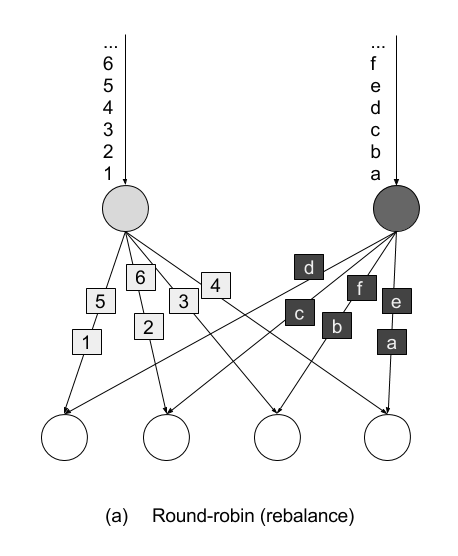
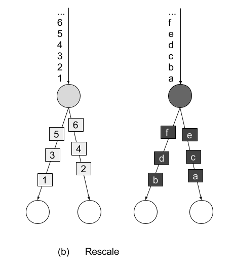
broadcast() method replicates the input data stream so that all events are sent to all parallel tasks of the downstream operator.
The global() method sends all events of the input data stream to the first parallel task of the downstream operator. This partitioning strategy must be used with care, as routing all events to the same task might impact the application performance.
When none of the predefined partitioning strategies is suitable, you can define your own custom partitioning strategy using the partitionCustom() method. The method receives a Partitioner object that implements the partitioning logic and the field or key position on which the stream is to be partitioned. The following example partitions a stream of integers so that all negative numbers are sent to the first task and all other numbers are sent to a random task:
val numbers: DataStream[(Int)] = ...
numbers.partitionCustom(myPartitioner, 0)

object myPartitioner extends Partitioner[Int] {
  val r = scala.util.Random

  override def partition(key: Int, numPartitions: Int): Int = {
    if (key < 0) 0 else r.nextInt(numPartitions)
  }
}
Flink applications are typically executed in a parallel environment, such as a cluster of machines. When a DataStream program is submitted to the JobManager for execution the system creates a dataflow graph and prepares the operators for execution. Each operator is split into one or multiple parallel tasks and each task processes a subset of the input stream. The number of parallel tasks of an operator is called the parallelism of the operator. You can control the operator parallelism of your Flink applications either by setting the parallelism at the execution environment or by setting the parallelism of individual operators.
The execution environment defines a default parallelism for all operators, data sources, and data sinks it executes. It is set using the StreamExecutionEnvironment.setParallelism() method. The following example shows how to set the default parallelism for all operators to 4:
// set up the streaming execution environmentvalenv=StreamExecutionEnvironment.getExecutionEnvironment// set default parallelism to 4env.setParallelism(4)
You can override the default parallelism of the execution environment by setting the parallelism of individual operators. In the following example, the source operator will be executed by 4 parallel tasks, the map transformation has parallelism 8, and the sink operation will be executed by 2 parallel tasks:
// set up the streaming execution environmentvalenv=StreamExecutionEnvironment.getExecutionEnvironment// set default parallelism to 4env.setParallelism(4)// the source has parallelism 4valresult:=env.addSource(newCustomSource)// set the map parallelism to 8.map(newMyMapper).setParallelism(8)// set the print sink parallelism to 2.().setParallelism(2)
Some of the transformations you have seen in the previous section require a key specification or field reference on the input stream type. In Flink, keys are not predefined in the input types like in systems that work with key-value pairs. Instead, keys are defined as functions over the input data. Therefore, it is not necessary to define data types to hold keys and values which avoids a lot of boilerplate code.
In the following we discuss different methods to reference fields and define keys on data types.
If the data type is a tuple, keys can be defined by simply using the field position of the corresponding tuple element. The following example keys the input stream by the second field of the input tuple:
valinput:DataStream[(Int,String,Long)]=...valkeyed=input.keyBy(1)
Composite keys consisting of more than one tuple fields can also be defined. In this case, the positions are provided as a list, one after the other. We can key the input stream by the second and third field as follows:
valkeyed2=input.keyBy(1,2)
Another way to define keys and select fields is by using String-based field expressions. Field expressions work for tuples, POJOs, and case classes. They also support the selection of nested fields.
In the introductory example of this chapter, we defined the following case class:
caseclassSensorReading(id:String,timestamp:Long,temperature:Double)
To key the stream by sensor id we can pass the field name “id" to the keyBy() function:
valsensorStream:DataStream[SensorReading]=...valkeyedSensors=sensorStream.keyBy("id")
POJO or case class fields are selected by their field name like in the above example. Tuple fields are referenced either by their field name (1-offset for Scala tuples, 0-offset of Java tuples) or by their 0-offset field index:
valinput:DataStream[(Int,String,Long)]=...valkeyed1=input.keyBy("2")// key by 3rd fieldvalkeyed2=input.keyBy("_1")// key by 1st field
DataStream<Tuple3<Integer,String,Long>>javaInput=...javaInput.keyBy(“f2”)// key Java tuple by 3rd field
Nested fields in POJOs and tuples are selected by denoting the nesting level with a “.”. Consider the following case classes for example:
caseclassAddress(address:String,zip:Stringcountry:String)caseclassPerson(name:String,birthday:(Int,Int,Int),// year, month, dayaddress:Address)
If we want to reference a person’s ZIP code, we can use the fields expression address.zip. It is also possible to nest expressions on mixed types: a fields expressions of birthday._1 references the first field of the birthday tuple, i.e., the year of birth. The full data type can be selected using the wildcard field expression _. For example birthday._ references the whole birthday tuple. The wildcard field expression is valid for all supported data types.
A third option to specify keys are KeySelector functions. A KeySelector function extracts a key from an input event.
// T: the type of input elements
// KEY: the type of the key
KeySelector[IN, KEY]
  > getKey(IN): KEY
The introductory example actually uses a simple KeySelector function in the keyBy() method:
valsensorData:DataStream[SensorReading]=...valbyId:KeyedStream[SensorReading,String]=sensorData.keyBy(_.id)
A KeySelector function receives an input item and returns a key. The key does not necessarily have to be a field of the input event but can be derived using arbitrary computations. In the following code example, the KeySelector function returns the maximum of the tuple fields as the key:
valinput:DataStream[(Int,Int)]=...valkeyedStream=input.keyBy(value=>math.max(value._1,value._2))
Compared to field positions and field expressions, an advantage of KeySelector functions is that the resulting key is strongly typed due to the generic types of the KeySelector class.
Most DataStream API methods accept UDFs in the form of lambda functions. Lambda functions are available for Scala and Java 8 and offer a simple and concise way to implement application logic when no advanced operations such as accessing state and configuration are required:
valtweets:DataStream[String]=...// a filter lambda function that checks if tweets contains the// word “flink”valflinkTweets=tweets.filter(_.contains("flink"))
A more powerful way to define UDFs are rich functions. Rich functions define additional methods for UDF initialization and teardown and provide hooks to access the context in which UDFs are executed. The previous lambda function example can be written using a rich function as follows:
classFlinkFilterFunctionextendsRichFilterFunction[String]{overridedeffilter(value:String):Boolean={value.contains("flink")}}
An instance of the rich function implementation can then be passed as an argument to the filter transformation:
valflinkTweets=tweets.filter(newFlinkFilterFunction)
Another way to define rich functions is as anonymous classes:
valflinkTweets=tweets.filter(newRichFilterFunction[String]{overridedeffilter(value:String):Boolean={value.contains(“flink”)}})
There exist rich versions of all the DataStream API transformation functions, so that you can use them in the same places where you can use a lambda function. The naming convention is that the function name starts with Rich followed by the transformation name, e.g. Filter and ends with Function, i.e. RichMapFunction, RichFlatMapFunction, and so on.
UDFs can receive parameters through their constructor. The parameters will be serialized with regular Java serialization as part of the function object and shipped to all the parallel task instances that will execute the function.
Flink serializes all UDFs with Java Serialization to ship them to the worker processes. Everything contained in a user function must be Serializable.
We can parametrize the above example and pass the string "flink" as a parameter to the FlinkFilterFunction constructor as shown below:
valtweets:DataStream[String]=…valflinkTweets=tweets.filter(newMyFilterFunction(“flink”))classMyFilterFunction(keyWord:String)extendsRichFilterFunction[String]{overridedeffilter(value:String):Boolean={value.contains(keyWord)}}
When using a rich function, you can implement two additional methods that provide access to the function’s lifecycle:
open() method is an initialization method for the rich function. It is called once per task before the transformation methods like filter, map, and fold are called. open() is typically used for setup work that needs to be done only once. Please note that the Configuration parameter is only used by the DataSet API and not by the DataStream API. Hence, it should be ignored.close() method is a finalization method for the function and it is called once per task after the last call of the transformation method. Thus, it is commonly used for cleanup and releasing resources.In addition, the method getRuntimeContext() provides access to the function’s RuntimeContext. The RuntimeContext can be used to retrieve information such as the function parallelism, its subtask index, and the name of the task where the UDF is currently being executed. Further, it includes methods for accessing partitioned state. Stateful stream processing in Flink is discussed in detail in Chapter 8. The following example code shows how to use the methods of a RichFlatMapFunction:
classMyFlatMapextendsRichFlatMapFunction[Int,(Int,Int)]{varsubTaskIndex=0overridedefopen(configuration:Configuration):Unit={subTaskIndex=getRuntimeContext.getIndexOfThisSubtask// do some initialization// e.g. establish a connection to an external system}overridedefflatMap(in:Int,out:Collector[(Int,Int)]):Unit={// subtasks are 0-indexedif(in%2==subTaskIndex){out.collect((subTaskIndex,in))}// do some more processing}overridedefclose():Unit={// do some cleanup, e.g. close connections to external systems}}
The open() and getRuntimeContext() methods can also be used for configuration via the environment ExecutionConfig. The ExecutionConfig can be retrieved using RuntimeContext’s getExecutionConfig() method and allows setting global configuration options which are accessible in all rich UDFs.
The following example program uses the global configuration to set the parameter keyWord to “flink" and then reads this parameter in a RichFilterFunction:
defmain(args:Array[String]):Unit={valenv=StreamExecutionEnvironment.getExecutionEnvironment// create a configuration objectvalconf=newConfiguration()// set the parameter “keyWord” to “flink”conf.setString("keyWord","flink")// set the configuration as globalenv.getConfig.setGlobalJobParameters(conf)// create some datavalinput:DataStream[String]=env.fromElements("I love flink","bananas","apples","flinky")// filter the input stream and print it to stdoutinput.filter(newMyFilterFunction).()env.execute()}classMyFilterFunctionextendsRichFilterFunction[String]{varkeyWord=""overridedefopen(configuration:Configuration):Unit={// retrieve the global configurationvalglobalParams=getRuntimeContext.getExecutionConfig.getGlobalJobParameters// cast to a Configuration objectvalglobConf=globalParams.asInstanceOf[Configuration]// retrieve the keyWord parameterkeyWord=globConf.getString("keyWord",null)}overridedeffilter(value:String):Boolean={// use the keyWord parameter to filter out elementsvalue.contains(keyWord)}}
Adding external dependencies is a common requirement when implementing Flink applications. There are many popular libraries out there, such as Apache Commons or Google Guava, which address and ease various use cases. Moreover, most Flink applications depend on one or more of Flink’s connectors to ingest data from or emit data to external systems, like Apache Kafka, file systems, or Apache Cassandra. Some applications also leverage Flink’s domain-specific libraries, such as the Table API, SQL, or the CEP library. Consequently, most Flink applications do not only depend on Flink’s DataStream API dependency and the Java SDK but also on additional third-party and Flink-internal dependencies.
When an application is executed, all its dependencies must be available to the application. By default, only the core API dependencies (DataStream and DataSet APIs) are loaded by a Flink cluster. All other dependencies that an application requires must be explicitly provided.
The reason for this design is to keep the number of default dependencies low2. Most connectors and libraries rely on one or more libraries, which typically have several additional transitive dependencies. Often, these include frequently used libraries, such as Apache Commons or Google’s Guava. Many problems originate from incompatibilities among different versions of the same library which are pulled in from different connectors or directly from the user application.
There are two approaches to ensure that all dependencies are available to an application when it is executed.
./lib folder of a Flink setup. In this case, the dependencies are loaded into the classpath when Flink processes are started. A dependency that is added to the classpath like this is available to (and might interfere with) all applications that run on the Flink setup.Building a so-called fat JAR file is the preferred way to handle application dependencies. Flink’s Maven archetypes that we introduced in Chapter 4 generate Maven projects that are configured to produce application fat JARs which include all required dependencies. Dependencies which are included in the classpath of Flink processes by default are automatically excluded from the JAR file. The pom.xml file contains comments that explain how to add additional dependencies.
In this chapter we have introduced the basics of Flink’s DataStream API. You have examined the structure of Flink programs and you have learnt how to combine data and partitioning transformations to build streaming applications. You have also looked into supported data types and different ways to specify keys and user-defined functions. If you now take a step back and read the introductory example once more, you hopefully have a clear idea about what is going on. In the next chapter, things are going to get even more interesting, as you learn how to enrich our programs with window operators and time semantics.
In this chapter, you will get an introduction to the DataStream API methods for time handling and time-based operators, as for example windows. As you learned in Chapter 2, Flink’s time-based operators can be applied with different notions of time.
In this chapter, you will first learn how to define time characteristics, timestamps, and watermarks. Then, you will learn about the ProcessFunction, a low-level transformation that provides access to record timestamps and watermarks and can register timers. Next, you will get to use Flink’s window API which provides built-in implementations of the most common window types. You will also get an introduction to custom, user-defined window operations and core windowing constructs, such as assigners, triggers, and evictors. Finally, we will discuss strategies to handle late events.
As you saw in Chapter 2, when defining time window operations in a distributed stream processing application, it is important to understand the meaning of time. When you specify a window to collect events in one-minute buckets, which events exactly will each bucket contain? In the DataStream API, you can use the time characteristic to instruct Flink how to reason about time when creating windows. The time characteristic is a property of the StreamExecutionEnvironment and it takes the following values:
ProcessingTime means that operators use the system clock of the machine where they are being executed to determine the current time of the data stream. Processing-time windows trigger based on machine time and include whatever elements happen to have arrived at the operator until that point in time. In general, using processing time for window operations results in non-deterministic results because the contents of the windows depend on the speed in which elements arrive. On the plus side, this setting offers very low latency because there is no such thing as out of order data for which operations would have to wait for.
EventTime means that operators determine the current time by using information from the data itself. Each event carries a timestamp and the logical time of the system is defined by watermarks. As you saw in Chapter 3, timestamps either exist in the data before entering the data processing pipeline, or they are assigned by the application at the sources. An event-time window triggers when a watermark informs it that all timestamps for a certain time interval have been received. Event-time windows compute deterministic results even when events arrive out-of-order. The window result will be the same and independent of how fast the stream is read or processed.
IngestionTime is a hybrid of of EventTime and ProcessingTime. The ingestion time of an event is the time when it entered the stream processor. You can think of ingestion time as assigning the processing time of the source operator as an event time timestamp to each ingested record. Ingestion time does not offer much practical value compared to event time as it does not provide deterministic results but has similar performance implications as event time.
We can see in Example 6-1 how to set the time characteristic by revisiting the sensor streaming application code you wrote in Chapter 5.
objectAverageSensorReadings{// main() defines and executes the DataStream programdefmain(args:Array[String]){// set up the streaming execution environmentvalenv=StreamExecutionEnvironment.getExecutionEnvironment// use event time for the applicationenv.setStreamTimeCharacteristic(TimeCharacteristic.EventTime)// ingest sensor streamvalsensorData:DataStream[SensorReading]=env.addSource(...)}}
Setting the time characteristic to EventTime enables record timestamps and watermark handling, and as a result event-time windows or operations. Of course, one can still use processing-time windows and timers if you choose the EventTime time characteristic.
To use processing time replace TimeCharacteristic.EventTime by TimeCharacteristic.ProcessingTime.
As discussed in Chapter 3, your application needs to provide two important pieces of information to Flink in order to operate in event time. Each event must be associated with a timestamp that typically indicates when the event actually happened. Moreover, event-time streams needs to carry watermarks from which operators infer the current event time.
Timestamps and watermarks are specified in milliseconds since the epoch of 1970-01-01T00:00:00Z. A watermark tells operators that no more events with a timestamp smaller or equal to the watermark must be expected. Timestamps and watermarks can be either assigned and generated by a SourceFunction or using an explicit user-defined timestamp assigner and watermark generator. Assigning timestamps and generating watermarks in a SourceFunction is discussed in Chapter 8. Here we explain how to do this with a user-defined function.
If a timestamp assigner is used, any existing timestamps and watermarks will be overwritten.
The DataStream API provides the TimestampAssigner interface to extract timestamps from elements after they have been ingested into the streaming application. Typically, the timestamp assigner is called right after the source function. That is because most assigners make assumption about the order of elements with respect to their timestamps to generate watermarks. Since elements are typically ingested in parallel, any operation that causes Flink to redistribute elements across parallel stream partitions, such as parallelism changes, keyBy(), or other explicit redistributions, mixes up the timestamp order of the elements.
It is best practice to assign timestamps and generate watermarks as close to the sources as possible or even within the SourceFunction. Depending on the use case, it is possible to apply an initial filtering or transformation on the input stream before assigning timestamp if such operations do not induce a redistribution of elements, e.g., by change the parallelism.
To ensure that event time operations behave as expected, the assigner should be called before any event-time dependent transformation, e.g. before the first event-time window.
Timestamp assigners behave like other transformation operators. They are called on a stream of elements and they produce a new stream of timestamped elements and watermarks. Note that if the input stream already contains timestamps and watermarks, those will be replaced by the timestamp assigner.
The code in Example 6-2 shows how to use timestamp assigners. In this example, after reading the stream, we first apply a filter transformation and then call the assignTimestampsAndWatermarks() method where we define the timestamp assigner MyAssigner(). Note how assigning timestamps and watermarks does not changes the type of the data stream.
valenv=StreamExecutionEnvironment.getExecutionEnvironment// set the event time characteristicenv.setStreamTimeCharacteristic(TimeCharacteristic.EventTime)// ingest sensor streamvalreadings:DataStream[SensorReading]=env.addSource(newSensorSource)// assign timestamps and generate watermarks.assignTimestampsAndWatermarks(newMyAssigner())
In the example above, MyAssigner can either be of type AssignerWithPeriodicWatermarks or AssignerWithPunctuatedWatermarks. These two interfaces extend the TimestampAssigner provided by the DataStream API. The first interface allows defining assigners that emit watermarks periodically while the second allows to inject watermarks based on a property of the input events. We describe both interfaces in detail next.
Assigning watermarks periodically means that we instruct the system to check the progress of event time in fixed intervals of machine time. The default interval is set to 200 milliseconds but it can be configured using the ExecutionConfig.setAutoWatermarkInterval() method as shown in Example 6-3.
valenv=StreamExecutionEnvironment.getExecutionEnvironmentenv.setStreamTimeCharacteristic(TimeCharacteristic.EventTime)// generate watermarks every 5 secondsenv.getConfig.setAutoWatermarkInterval(5000)
In the above example, you instruct the program to check the current watermark value every 5 seconds. What actually happens is that every 5 seconds Flink invokes the getCurrentWatermark() method of AssignerWithPeriodicWatermarks. If the method returns a non-null value with a timestamp larger than the timestamp of the previous watermark, then the new watermark is forwarded. Note that this check is necessary to ensure that event time continuously increases. Otherwise, if the method returns a null value or the timestamp of the returned watermark is smaller than that of the last emitted one, no watermark is produced.
Example 6-4 shows an assigner with periodic timestamps which produces watermarks by keeping track of the maximum element timestamp it has seen so far. When being asked for a new watermark, the assigner returns a watermark with the maximum timestamp minus a 1 minute tolerance interval.
classPeriodicAssignerextendsAssignerWithPeriodicWatermarks[SensorReading]{valbound:Long=60*1000// 1 min in msvarmaxTs:Long=Long.MinValue// the maximum observed timestampoverridedefgetCurrentWatermark:Watermark={// generated watermark with 1 min tolerancenewWatermark(maxTs-bound)}overridedefextractTimestamp(r:SensorReading,previousTS:Long):Long={// update maximum timestampmaxTs=maxTs.max(r.timestamp)// return record timestampr.timestamp}}
The DataStream API provides implementations for two common cases of timestamp assigners with periodic watermarks. If your input elements have timestamps which are monotonously increasing, you can use the shortcut method assignAscendingTimestamps. This method uses the current timestamp to generate watermarks, since no earlier timestamps can appear. Example 6-5 shows how to generate watermarks for ascending timestamps.
valstream:DataStream[MyEvent]=...valwithTimestampsAndWatermarks=stream.assignAscendingTimestamps(e=>e.getCreationTime)
The other common case of periodic watermark generation is when you know the maximum lateness that you will encounter in the input stream, that is the maximum difference between an element’s timestamp and the largest timestamp of all perviously ingested elements. For such cases, Flink provides the BoundedOutOfOrdernessTimestampExtractor which takes the maximum expected lateness as an argument.
valstream:DataStream[MyEvent]=...valoutput=stream.assignTimestampsAndWatermarks(newBoundedOutOfOrdernessTimestampExtractor[MyEvent](Time.seconds(10))(_.getCreationTime)
In Example 6-6 elements are allowed to be late for 10 seconds. That is, if the difference between an element’s event time and the maximum timestamp of all previous elements is greater than 10 seconds, the element might arrive after a related computation has completed and result has been emitted. Flink offers different strategies to handle such late events and we discuss those later in this chapter.
Sometimes the input stream contains special tuples or markers that indicate the stream’s progress. For such cases or when watermarks can be defined based on some other property of the input elements, Flink provides the AssignerWithPunctuatedWatermarks. The interface contains the checkAndGetNextWatermark() method which is called for each event right after extractTimestamp(). The method can decide to generate a new watermark or not. A new watermark is emitted if the method returns a non-null watermark which is larger than the latest emitted watermark.
Example 6-7 shows a punctuated watermark assigner that emits a watermark for every reading that it rececives from the sensor with the id "sensor_1".
classPunctuatedAssignerextendsAssignerWithPunctuatedWatermarks[SensorReading]{valbound:Long=60*1000// 1 min in msoverridedefcheckAndGetNextWatermark(r:SensorReading,extractedTS:Long):Watermark={if(r.id=="sensor_1"){// emit watermark if reading is from sensor_1newWatermark(extractedTS-bound)}else{// do not emit a watermarknull}}overridedefextractTimestamp(r:SensorReading,previousTS:Long):Long={// assign record timestampr.timestamp}}
So far we discussed how to generate watermarks using a TimestampAssigner. What we have not discussed yet is the effect that watermarks have on your streaming application.
Watermarks are a mechanism to trade-off result latency and result completeness. They control how long to wait for data to arrive before performing a computation, such as finalizing a window computation and emitting the result. An operator that is based on event time uses watermarks to determine the completeness of its ingested records and the progress of its operation. Based on watermarks the operator computes a point in time up at which it expects to have received all records with a smaller timestamp.
However, the distributed systems’ reality is that we can never have perfect watermarks. That would mean we are always certain that there are no delayed records. In practice, you need to make an educated guess and use heuristics to generate watermarks in your applications. Commonly, you need to use whatever information you have about the sources, the network, the partitions to estimate progress and probably also an upper bound of lateness for your input records. Estimates mean there is room for errors in which case you might generate watermarks that are inaccurate, resulting into late data or unnecessary increase in the application’s latency. With this in mind, you can use watermarks to trade-off the result latency and result completeness of an application.
If you generate loose watermarks, i.e., the watermarks are far behind the timestamps of the processed records, you increase the latency of produced results. You could have generated a result earlier but you had to wait for the watermark. Moreover the state size typically increases because the application needs to buffer more data until it can perform a computation. However, you can be quite certain that all relevant data is available when you perform a computation.
On the other hand, if you generate very tight watermark, i.e., watermarks that might be larger than the timestamps of some later arriving records, time-based operations might be performed before all relevant data has arrived. You should have waited longer to receive delayed events before performing the computation. While this might yield incomplete or inaccurate results, the results are produced in a timely fashion with lower latency.
The latency-completeness tradeoff is a fundamental charateristic of stream processing that is not relevant for batch applications, which are built around the premise that all data is available. Watermarks are a powerful feature to control the behavior of an application with respect to time. Besides watermarks, Flink provides many knobs to tweak the exact behavior of time-based operations, such as window Triggers and the ProcessFunction, and offers different ways to handle late data, i.e., elements that arrived after a computation was performed. We will discuss these features in a dedicated section at the end of this chapter.
Even though time information and watermarks are crucial to many streaming applications, you might have noticed that we cannot access them through the basic DataStream API transformations that we have seen so far. For example, a MapFunction does not have access to time-related constructs.
The DataStream API provides a family of low-level transformations, the process functions, which can also access record timestamps and watermarks and register timers that trigger at a specific time in the future. Moreover, process functions feature side outputs to emit records to multiple output streams. Process functions are commonly used to build event-driven applications and to implement custom logic for which predefined windows and transformations might not be suitable. For example most of operators for Flink’s SQL support are implemented using process functions.
Currently, Flink provides seven different process functions: ProcessFunction, KeyedProcessFunction, CoProcessFunction, BroadcastProcessFunction, KeyedBroadcastProcessFunction, ProcessWindowFunction, and ProcessAllWindowFunction. As indicated by the name, these functions are applicable in different contexts. However, they have a very similar features set. We continue discussing the common features by looking in detail at the ProcessFunction.
The ProcessFunction is a very versatile function and can be applied to a regular DataStream and to a KeyedStream. The function is called for each record of the stream and can return zero, one, or more records. All process functions implement the RichFunction interface and hence offer its open() and close() methods. Additionally, the ProcessFunction provides the following two methods:
processElement(v: IN, ctx: Context, out: Collector[OUT]) is called for each record of the stream. As usual, result records are emitted by passing them to the Collector. The Context object is what makes the ProcessFunction special. It gives access to the timestamp of the current record and to a TimerService. Moreover, the Context can emit records to side outputs.
onTimer(timestamp: Long, ctx: OnTimerContext, out: Collector[OUT]) is a callback function that is invoked when a previously registered timer triggers. The timestamp argument gives the timestamp of the firing timer and the Collector allows to emit records. The OnTimerContext provides the same services as the Context object of the processElement() method and it returns the time domain (processing time or event time) of the firing trigger in addition.
The TimerService of the Context and OnTimerContext objects offer the following methods:
currentProcessingTime(): Long returns the current processing time.currentWatermark(): Long returns the timestamp of the current watermark.registerProcessingTimeTimer(timestamp: Long): Unit registers a processing time timer. The timer will fire when the processing time of the executing machine reaches the provided timestamp.registerEventTimeTimer(timestamp: Long): Unit registers an event time timer. The timer will fire when the watermark is updated to a timestamp that is equal to or larger than the timer’s timestamp.When a timer fires, the onTimer() callback function is called. The processElement() and onTimer() methods are synchronized to prevent concurrent access and manipulation of state. Note that timers can only be registered on keyed streams.
To use timers on a non-keyed stream, you can create a keyed stream by using a KeySelector with a constant dummy key. Note that this will move all data to a single task such that the operator would be effectively executed with a parallelism of 1.
For each key and timestamp, one timer can be registered, i.e., each key can have multiple timers but only one for each timestamp. It is not possible to delete registered timers. Internally, a ProcessFunction holds the timestamps of all timers in a priority queue on the heap and persists them as function state of type Long. A common use case for timers is to clear keyed state after some period of inactivity for a key or to implement custom time-based windowing logic.
Timers are checkpointed along with any other state of the function. If an application needs to recover from a failure, all processing time timers that expired while the application was restarting will fire immediately when the application resumes. This is also true for processing time timers that are persisted in a savepoint. Note that timers are currently not asynchronously checkpointed. Hence, a ProcessFunction with many timers can significantly increase the checkpointing time. It is best practice to not use timers overly excessive.
Example 6-8 shows a ProcessFunction that monitors the temperatures of sensors and emits a warning if the temperature of a sensor monotonically increases for a period of 1 second in processing time.
valwarnings=readings// key by sensor id.keyBy(_.id)// apply ProcessFunction to monitor temperatures.process(newTempIncreaseAlertFunction)// =================== ///** Emits a warning if the temperature of a sensor* monotonically increases for 1 second (in processing time).*/classTempIncreaseAlertFunctionextendsKeyedProcessFunction[String,SensorReading,String]{// hold temperature of last sensor readinglazyvallastTemp:ValueState[Double]=getRuntimeContext.getState(newValueStateDescriptor[Double]("lastTemp",Types.of[Double]))// hold timestamp of currently active timerlazyvalcurrentTimer:ValueState[Long]=getRuntimeContext.getState(newValueStateDescriptor[Long]("timer",Types.of[Long]))overridedefprocessElement(r:SensorReading,ctx:KeyedProcessFunction[String,SensorReading,String]#Context,out:Collector[String]):Unit={// get previous temperaturevalprevTemp=lastTemp.value()// update last temperaturelastTemp.update(r.temperature)if(prevTemp==0.0||r.temperature<prevTemp){// temperature decreased. Invalidate current timercurrentTimer.update(0L)}elseif(r.temperature>prevTemp&¤tTimer.value()==0){// temperature increased and we have not set a timer yet.// set processing time timer for now + 1 secondvaltimerTs=ctx.timerService().currentProcessingTime()+1000ctx.timerService().registerProcessingTimeTimer(timerTs)// remember current timercurrentTimer.update(timerTs)}}overridedefonTimer(ts:Long,ctx:KeyedProcessFunction[String,SensorReading,String]#OnTimerContext,out:Collector[String]):Unit={// check if firing timer is current timerif(ts==currentTimer.value()){out.collect("Temperature of sensor '"+ctx.getCurrentKey+"' monotonically increased for 1 second.")// reset current timercurrentTimer.update(0)}}}
Most operators of the DataStream API have a single output, i.e, they produce one result stream with a specific data type. Only the split operator allows to split a stream into multiple streams of the same type. Side outputs are a mechanism to emit multiple streams from a function with possibly different types. The number of side outputs besides the primary output is not limited. Each individual side output is identified by an OutputTag[X] object which is instantiated with a name and the type X of the side output stream. A ProcessFunction can emit a record to one or more side outputs via a Context object.
Example 6-9 shows a ProcessFunction that monitors a stream of sensor readings and emits a warning to a side output for readings with a temperature below 32F.
// define a side output tagvalfreezingAlarmOutput:OutputTag[String]=newOutputTag[String]("freezing-alarms")// =================== //valmonitoredReadings:DataStream[SensorReading]=readings// monitor stream for readings with freezing temperatures.process(newFreezingMonitor)// retrieve and print the freezing alarmsmonitoredReadings.getSideOutput(freezingAlarmOutput).()// print the main outputreadings.()// =================== ///** Emits freezing alarms to a side output for readings* with a temperature below 32F. */classFreezingMonitorextendsProcessFunction[SensorReading,SensorReading]{overridedefprocessElement(r:SensorReading,ctx:ProcessFunction[SensorReading,SensorReading]#Context,out:Collector[SensorReading]):Unit={// emit freezing alarm if temperature is below 32F.if(r.temperature<32.0){ctx.output(freezingAlarmOutput,s"Freezing Alarm for${r.id}")}// forward all readings to the regular outputout.collect(r)}}
For low-level operations on two inputs, the Datastream API also provides the CoProcessFunction. Similar to a CoFlatMapFunction, a CoProcessFunction offers a transformation method for each input, processElement1() and processElement2(). Similar to the ProcessFunction, both methods are called with a Context object that gives access to the element or timer timestamp, a TimerService, and side outputs. The CoProcessFunction also provides a onTimer() callback method.
Example 6-10shows a CoProcessFunction that dynamically filters a stream of sensor readings based on a stream of filter switches.
// ingest sensor streamvalsensorData:DataStream[SensorReading]=...// filter switches enable forwarding of readingsvalfilterSwitches:DataStream[(String,Long)]=env.fromCollection(Seq(("sensor_2",10*1000L),// forward sensor_2 for 10 seconds("sensor_7",60*1000L))// forward sensor_7 for 1 minute)valforwardedReadings=readings// connect readings and switches.connect(filterSwitches)// key by sensor ids.keyBy(_.id,_._1)// apply filtering CoProcessFunction.process(newReadingFilter)// =============== //classReadingFilterextendsCoProcessFunction[SensorReading,(String,Long),SensorReading]{// switch to enable forwardinglazyvalforwardingEnabled:ValueState[Boolean]=getRuntimeContext.getState(newValueStateDescriptor[Boolean]("filterSwitch",Types.of[Boolean]))// hold timestamp of currently active disable timerlazyvaldisableTimer:ValueState[Long]=getRuntimeContext.getState(newValueStateDescriptor[Long]("timer",Types.of[Long]))overridedefprocessElement1(reading:SensorReading,ctx:CoProcessFunction[SensorReading,(String,Long),SensorReading]#Context,out:Collector[SensorReading]):Unit={// check if we may forward the readingif(forwardingEnabled.value()){out.collect(reading)}}overridedefprocessElement2(switch:(String,Long),ctx:CoProcessFunction[SensorReading,(String,Long),SensorReading]#Context,out:Collector[SensorReading]):Unit={// enable reading forwardingforwardingEnabled.update(true)// set disable forward timervaltimerTimestamp=ctx.timerService().currentProcessingTime()+switch._2ctx.timerService().registerProcessingTimeTimer(timerTimestamp)disableTimer.update(timerTimestamp)}overridedefonTimer(ts:Long,ctx:CoProcessFunction[SensorReading,(String,Long),SensorReading]#OnTimerContext,out:Collector[SensorReading]):Unit={if(ts==disableTimer.value()){// remove all state. Forward switch will be false by default.forwardingEnabled.clear()disableTimer.clear()}}}
Windows are common operations in streaming applications. Windows enable transformations on bounded intervals of an unbounded stream, such as aggregations. Typically, these intervals are defined using time-based logic. Window operators provide a way to group events in buckets of finite size and apply computations on the bounded contents of these buckets. For example, a window operator can group the events of a stream into windows of 5 minutes and count for each window how many events have been received.
The DataStream API provides built-in methods for the most common window operations as well as a very flexible windowing mechanism to define custom windowing logic. In this section we show you how to define window operators, present the built-in window types of the DataStream API, discuss the functions that can be applied on a window, and finally explain how to define custom windowing logic.
Window operators can be applied on a keyed or a non-keyed stream. Window operators on keyed windows are evaluated in parallel, non-keyed windows are processed in a single thread.
To create a window operator, you need to specify two window components.
WindowedStream (or AllWindowedStream if applied on a non-keyed DataStream).WindowedStream (or AllWindowedStream) and processes the elements which are assigned to a window.// define a keyed window operatorstream.keyBy(...).window(...)// specify the window assigner.reduce/aggregate/process(...)// specify the window function// define a non-keyed window-all operatorstream.windowAll(...)// specify the window assigner.reduce/aggregate/process(...)// specify the window function
In the remainder of the chapter we focus on keyed windows only. Non-keyed windows (also called all-windows in the DataStream API) behave exactly the same, except that they are not evaluated in parallel.
Note that you can customize a window operator by providing a custom Trigger or Evictor and declaring strategies for how to deal with late elements. Custom window operators are dicussed in detail later in this section.
Flink provides built-in window assigners for the most common windowing use cases. All assigners that we discuss here are time-based and were introduced in Chapter 2. Time-based window assigners assign an element based on its the event-time timestamp or the current processing time to windows. Time windows have a start and an end timestamp.
All built-in windows assigners provide a default trigger that triggers the evaluation of a window once the (processing or event) time passes the end of the window. It is important to note that a window is created when the first element is assigned to it. Hence, Flink will never evaluate empty windows.
In addition to time-based windows, Flink also supports count-based windows, i.e., windows that group a fixed number of elements in the order in which they arrive at the window operator. Since they depend on the ingestion order, count-based windows are not deterministic. Moreover, they can cause issues if they are used without a custom Trigger that discards incomplete and stale windows at some point.
Flink’s built-in window assigners create windows of type TimeWindow. This window type essentially represents a time interval between the two timestamps, where start is inclusive and end is exclusive. It exposes methods to retrieve the window boundaries, to check whether windows intersect, and to merge overlapping windows.
In the following, we show the different built-in window assigners of the DataStream API and how to use them to define window operators.
A tumbling window assigner places elements to non-overlapping, fixed-size windows, as shown in the Figure Figure 6-1.
The Datastream API provides two assigners, TumblingEventTimeWindows and TumblingProcessingTimeWindows for tumbling event-time and processing-time windows, respectively. A tumbling windows assigner receives one parameter which is the window size in time units and can be specified using the of(Time size) method of the assigner. The time interval can be set in milliseconds, seconds, minutes, hours, or days.
Example 6-12 and Example 6-13 show how to define event-time and processing-time tumbling windows on a stream of sensor data measurements.
valsensorData:DataStream[SensorReading]=...valavgTemp=sensorData.keyBy(_.id)// group readings in 1s event-time windows.window(TumblingEventTimeWindows.of(Time.seconds(1))).process(newTemperatureAverager)
valavgTemp=sensorData.keyBy(_.id)// group readings in 1s processing-time windows.window(TumblingProcessingTimeWindows.of(Time.seconds(1))).process(newTemperatureAverager)
If you remember this example when we first encountered it in Chapter 2, the window definition looked a bit different. Back then, we defined an event-time tumbling window using the timeWindow(size) method, which is a shortcut for window.(TumblingEventTimeWindows.of(size)) or window.(TumblingProcessingTimeWindows.of(size)) depending on the configured time characteristic.
valavgTemp=sensorData.keyBy(_.id)// shortcut for window.(TumblingEventTimeWindows.of(size)).timeWindow(Time.seconds(1)).process(newTemperatureAverager)
By default, tumbling windows are aligned to the epoch time, i.e., 1970-01-01-00:00:00.000. For example, an assigner with a size of one hour will define windows at 00:00:00, 01:00:00, 02:00:00 and so on. Alternatively, you can specify an offset as a second parameter in the assigner. The example in Example 6-15 shows windows with an offset of 15 minutes that start at 00:15:00, 01:15:00, 02:15:00, etc.
valavgTemp=sensorData.keyBy(_.id)// group readings in 1 hour windows with 15 min offset.window(TumblingEventTimeWindows.of(Time.hours(1),Time.minutes(15))).process(newTemperatureAverager
The sliding window assigner places stream elements to possibly overlapping, fixed-size windows, as shown in Figure Figure 6-2.
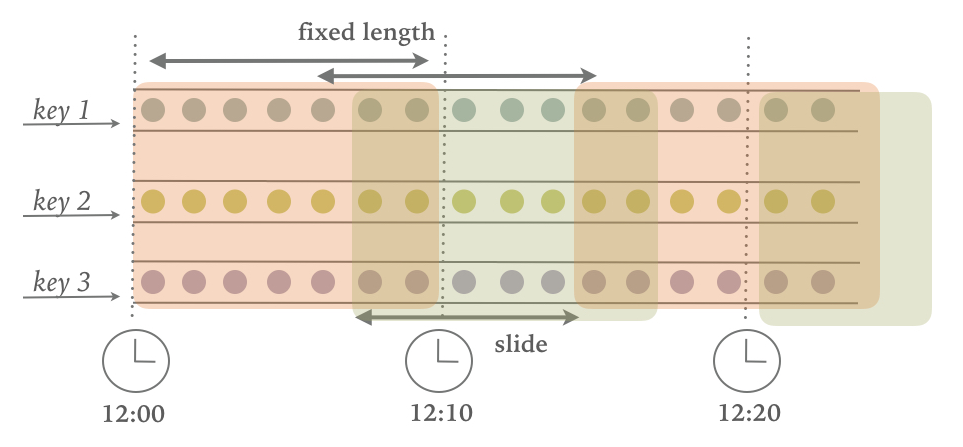
For a sliding window, you have to specify a window size and a slide interval that defines how frequently a new window is started. When the slide interval is smaller than the window size, the windows overlap and elements be assigned to more than one window. If the slide is larger than the window size, some elements might not be assigned to any window and hence be dropped.
Example 6-16 shows how to group the sensor readings in sliding windows of 1 hour and 15 minutes slide. Each reading will be added to four windows. The DataStream API provides event-time and processing-time assigners, as well as shortcut methods, while a time interval offset can be set as the third parameter to the window assigner.
// event-time sliding windows assignervalslidingAvgTemp=sensorData.keyBy(_.id)// create 1h event-time windows every 15 minutes.window(SlidingEventTimeWindows.of(Time.hours(1),Time.minutes(15))).process(newTemperatureAverager)// processing-time sliding windows assignervalslidingAvgTemp=sensorData.keyBy(_.id)// create 1h processing-time windows every 15 minutes.window(SlidingProcessingTimeWindows.of(Time.hours(1),Time.minutes(15))).process(newTemperatureAverager)// sliding windows assigner using a shortcut methodvalslidingAvgTemp=sensorData.keyBy(_.id)// shortcut for window.(TumblingEventTimeWindows.of(size)).timeWindow(Time.hours(1),Time(minutes(15))).process(newTemperatureAverager
A session window assigner places elements into non-overlapping windows of activity that have no fixed size. The boundaries of a session windows are defined by gaps of inactivity, i.e., time intervals in which no record is received. Figure Figure 6-3illustrates how elements are assigned to session windows.
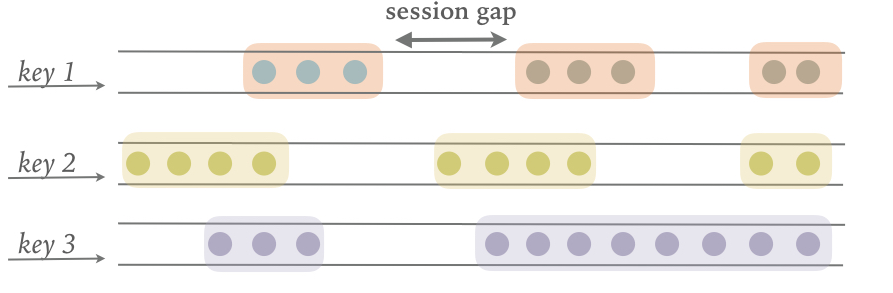
The following examples show how to group the sensor readings into session windows where a session is defined by a 15 min period of inactivity:
// event-time session windows assignervalsessionWindows=sensorData.keyBy(_.id)// create event-time session windows with a 15 min gap.window(EventTimeSessionWindows.withGap(Time.minutes(15))).process(...)// processing-time session windows assignervalsessionWindows=sensorData.keyBy(_.id)// create processing-time session windows with a 15 min gap.window(ProcessingTimeSessionWindows.withGap(Time.minutes(15))).process(...)
Since session windows do not have predefined start and end timestamps, a window assigner cannot immediately assign them to the correct window. Therefore, the SessionWindows assigner initially maps each incoming element into its own window with the element’s timestamp as the start time and the session gap as the window size. Subsequently, it merges all windows with overlapping ranges
Window functions define the computation that is performed on the elements of a window. There are two types of functions that can be applied on window.
ReduceFunction and AggregateFunction are incremental aggregation functions.ProcessWindowFunction is a full window function.In this section, we discuss the different types of functions that can be applied on a window to perform aggregations or arbitrary computations on the window’s contents. We also show how to jointly apply incremental aggregation and full window functions in a window operator.
The ReduceFunction was introduced in Chapter 5 when discussing running aggregations on keyed streams. A ReduceFunction accepts two values of the same type and combines them into a single value of the same type. When being applied on a windowed stream, a ReduceFunction incrementally aggregates the elements that are assigned to a window. A window only stores the current result of the aggregation, i.e., a single value of the ReduceFunction’s input (and output) type. When a new element is received, the ReduceFunction is called with the new element and the result that is read from the window’s state. The window’s state is replaced by the ReduceFunction’s result.
The advantages of applying a ReduceFunction on a window is the constant and small state size per window and the simple function interface. However, the applications for a ReduceFunction are limited and usually restricted to simple aggregations since the input and output type must be the same.
ReduceFunction that computes the mininum temperature per sensor and 15 seconds window.
valminTempPerWindow:DataStream[(String,Double)]=sensorData.map(r=>(r.id,r.temperature)).keyBy(_._1).timeWindow(Time.seconds(15)).reduce((r1,r2)=>(r1._1,r1._2.min(r2._2)))
For Example 6-18, we use a lambda function to specify how two elements of a window can be combined to produce an output of the same type. The same example can also be implemented with a class that implements the ReduceFunction interface as shows in Example 6-19.
valminTempPerWindow:DataStream[(String,Double)]=sensorData.map(r=>(r.id,r.temperature)).keyBy(_._1).timeWindow(Time.seconds(15)).reduce(newMinTempFunction)// ================ //// A reduce function to compute the minimum temperature per sensor.classMinTempFunctionextendsReduceFunction[(String,Double)]{overridedefreduce(r1:(String,Double),r2:(String,Double))={(r1._1,r1._2.min(r2._2))}}
Similar to a ReduceFunction, an AggregateFunction is also incrementally applied to the elements that are applied to a window. Moreover, also the state of a window with an AggregateFunction consists of a single value.
However, the interface of the AggregateFunction is much more flexible but also more complex to implement compared to the interface of the ReduceFunction. Example 6-20 shows the interface of the AggregateFunction.
publicinterfaceAggregateFunction<IN,ACC,OUT>extendsFunction,Serializable{// create a new accumulator to start a new aggregate.ACCcreateAccumulator();// add an input element to the accumulator and return the accumulator.ACCadd(INvalue,ACCaccumulator);// compute the result from the accumulator and return it.OUTgetResult(ACCaccumulator);// merge two accumulators and return the result.ACCmerge(ACCa,ACCb);}
The interface defines a type for input elements, IN, an accumulator of type ACC, and a result type OUT. In contrast to the ReduceFunction, the intermediate data type and the output type do not depend on the input type.
AggregateFunction to compute the average temperature of sensor readings per window. The accumulator maintains a running sum and count and the getResult() method computes the average value.
valavgTempPerWindow:DataStream[(String,Double)]=sensorData.map(r=>(r.id,r.temperature)).keyBy(_._1).timeWindow(Time.seconds(15)).aggregate(newAvgTempFunction)// ========= //// An AggregateFunction to compute the average tempeature per sensor.// The accumulator holds the sum of temperatures and an event count.classAvgTempFunctionextendsAggregateFunction[(String,Double),(String,Double,Int),(String,Double)]{overridedefcreateAccumulator()={("",0.0,0)}overridedefadd(in:(String,Double),acc:(String,Double,Int))={(in._1,in._2+acc._2,1+acc._3)}overridedefgetResult(acc:(String,Double,Int))={(acc._1,acc._2/acc._3)}overridedefmerge(acc1:(String,Double,Int),acc2:(String,Double,Int))={(acc1._1,acc1._2+acc2._2,acc1._3+acc2._3)}}
ReduceFunction and AggregateFunction are incrementally applied on events that are assigned to a window. However, sometimes we need access to all elements of a window to perform more complex computations, such as computing the the median of values in a window or the most frequently occurring value. For such applications, neither the ReduceFunction nor the AggregateFunction are suitable. Flink’s DataStream API offers the ProcessWindowFunction to perform arbitrary computations on the contents of a window.
The DataStream API of Flink 1.5 features the WindowFunction interface. WindowFunction has been superseded by ProcessWindowFunction and will not be discussed here.
ProcessWindowFunction.
publicabstractclassProcessWindowFunction<IN,OUT,KEY,WextendsWindow>extendsAbstractRichFunction{// Evaluates the window.voidprocess(KEYkey,Contextctx,Iterable<IN>vals,Collector<OUT>out)throwsException;// Deletes any custom per-window state when the window is purged.publicvoidclear(Contextctx)throwsException{}// The context holding window metadata.publicabstractclassContextimplementsSerializable{// Returns the metadata of the windowpublicabstractWwindow();// Returns the current processing time.publicabstractlongcurrentProcessingTime();// Returns the current event-time watermark.publicabstractlongcurrentWatermark();// State accessor for per-window state.publicabstractKeyedStateStorewindowState();// State accessor for per-key global state.publicabstractKeyedStateStoreglobalState();// Emits a record to the side output identified by the OutputTag.publicabstract<X>voidoutput(OutputTag<X>outputTag,Xvalue);}}
The process() method is called with the key of the window, an Iterable to access the elements of the window, and a Collector to emit results. Moreover, the method has a Context parameter similar to other process methods. The Context object of the ProcessWindowFunction gives access to meta data of the window, the current processing time and watermark, state stores to manage per-window and per-key global state, as well as side outputs to emit records.
We already discussed some of the features of the Context object when introducing the ProcessFunction, such as access to the current processing and event time and side outputs. However, ProcessWindowFunction’s Context object also offers a unique feature. The meta data of the window typically contains information that can be used as an identifier for a window, such as the start and end timestamps in case of a time window.
Another feature are per-window and per-key global state. Global state refers to the keyed state that is not scoped to any window, while per-window state refers to the window instance that is currently being evaluated. Per-window state is useful to maintain information that should be shared between multiple invocations of the process() method on the same window, which can happen due to configuring allowed lateness or using a custom Trigger. A ProcessWindowFunction that utilizes per-window state needs to implement its clear() method to clean up any window-specific state before the window is purged. Global state can be used to share information between multiple windows on the same key.
ProcessWindowFunction to compute the lowest and the highest temperature that occurs within the window. It then outputs the start and end timestamp of each window, followed by these two temperature values:
// output the lowest and highest temperature reading every 5 secondsvalminMaxTempPerWindow:DataStream[MinMaxTemp]=sensorData.keyBy(_.id).timeWindow(Time.seconds(5)).process(newHighAndLowTempProcessFunction)// ========= //caseclassMinMaxTemp(id:String,min:Double,max:Double,endTs:Long)/*** A ProcessWindowFunction that computes the lowest and highest temperature* reading per window and emits a them together with the* end timestamp of the window.*/classHighAndLowTempProcessFunctionextendsProcessWindowFunction[SensorReading,MinMaxTemp,String,TimeWindow]{overridedefprocess(key:String,ctx:Context,vals:Iterable[SensorReading],out:Collector[MinMaxTemp]):Unit={valtemps=vals.map(_.temperature)valwindowEnd=ctx.window.getEndout.collect(MinMaxTemp(key,temps.min,temps.max,windowEnd))}}
Internally, a window that is evaluated by ProcessWindowFunction stores all assigned events in a ListState1. By collecting all events and providing access to window meta data and other features, the ProcessWindowFunction can address many more use cases than a ReduceFunction or AggregateFunction. However, the state of a window that collects all events can become significantly larger than the state of a window whose elements are incrementally aggregated.
The ProcessWindowFunction is a very powerful window function but you need to use it with caution since it typically holds more data in state than incrementally aggregating functions. In fact it is quite common, that most of the logic that needs be applied on a window can be expressed as an incremental aggregation but it also need access to window metadata or state.
In such a case, you can combine a ReduceFunction or AggregateFunction, which performs incremental aggreagtion, with a ProcessWindowFunction that provides access to more functionality. Elements that are assigned to a window will be immediately processed and when the Trigger of the window fires, the aggregated result will be handed to the ProcessWindowFunction. The Iterable parameter of the ProcessWindowFunction.process() method will only provide a single value, the incrementally aggregated result.
In the DataStream API this is done by providing a ProcessWindowFunction as a second parameter to the reduce() or aggregate() methods as shown in Example 6-24 and Example 6-25.
input.keyBy(...).timeWindow(...).reduce(incrAggregator:ReduceFunction[IN],function:ProcessWindowFunction[IN,OUT,K,W])
input.keyBy(...).timeWindow(...).aggregate(incrAggregator:AggregateFunction[IN,ACC,V],windowFunction:ProcessWindowFunction[V,OUT,K,W])
The example in Example 6-26 shows how to solve the same use case as the code in Example 6-23 with a combination of a ReduceFunction and a ProcessWindowFunction, i.e., how to emit every 5 seconds the minimun and maximum temperature per sensor and the end timestamp of each window.
valminMaxTempPerWindow2:DataStream[MinMaxTemp]=sensorData.map(r=>(r.id,r.temperature,r.temperature)).keyBy(_._1).timeWindow(Time.seconds(5)).reduce(// incrementally compute min and max temperature(r1:(String,Double,Double),r2:(String,Double,Double))=>{(r1._1,r1._2.min(r2._2),r1._3.max(r2._3))},// finalize result in ProcessWindowFunctionnewAssignWindowEndProcessFunction())// ========= //caseclassMinMaxTemp(id:String,min:Double,max:Double,endTs:Long)classAssignWindowEndProcessFunctionextendsProcessWindowFunction[(String,Double,Double),MinMaxTemp,String,TimeWindow]{overridedefprocess(key:String,ctx:Context,minMaxIt:Iterable[(String,Double,Double)],out:Collector[MinMaxTemp]):Unit={valminMax=minMaxIt.headvalwindowEnd=ctx.window.getEndout.collect(MinMaxTemp(key,minMax._2,minMax._3,windowEnd))}}
Window operators that are defined using Flink’s built-in window assigners can address many common business use cases. However, as you start writing more advanced streaming applications, you might find yourself in the need to implement more complex windowing logic, such as windows that emit early results, update their result if late elements are encountered, or windows that start and end when specific records are received.
The DataStream API exposes interfaces and methods to define custom window operators by implementing your own assigners, triggers, and evictors. Together with the previously discussed window functions, these components work together in a window operator to group and process elements in windows.
When an element arrives at a window operator, it is handed to the WindowAssigner. The assigner determines to which windows the element needs to be routed. If a window does not exist yet, it is created.
If the window operator is configured with an incremental aggregation function, such as a ReduceFunction or AggregateFunction, the newly added element is immediately aggregated and the result is stored as the contents of the window. If the window operator does not have an incremental aggregation function, the new element is appended to a ListState that holds all assigned elements.
Everytime an element is added to a window, it is also passed to the Trigger of the window. The trigger defines (fires) when a window is considered ready for evaluation and when a window is purged and its contents is cleared. A trigger can decide based on assigned elements or register timers (similar to a process function) to evaluate or purge the content of its window at specific points in time.
What happens when a trigger fires, depends on the configured functions of the window operator. If the operator is configured just with an incremental aggregation function, the current aggregation result is emitted. This case is visualized in Figure Figure 6-4.
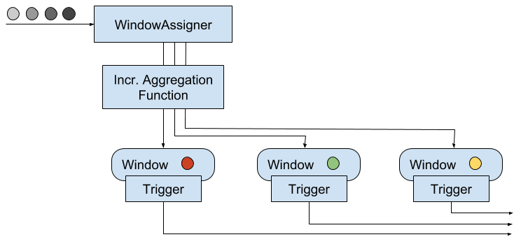
If the operator only has a full window function, the function is applied on all elements of the window and the result is emitted as shown by Figure Figure 6-5.
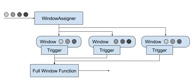
Finally, if the operator has an incremental aggregation function and a full window function, the full window function is applied on the aggregated value and the result is emitted. Figure Figure 6-6 depicts this case.
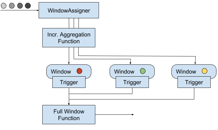
The Evictor is an optional component, that can be injected before or after a ProcessWindowFunction is called. An evictor can remove collected elements from the content of a window. Since it has to iterate over all elements, it can only be used if no incremental aggregation function is specified.
Example 6-27 shows how to define a window operator with a custom trigger and evictor.
stream.keyBy(...).window(...)// specify the window assigner[.trigger(...)]// optional: specify the trigger[.evictor(...)]// optional: specify the evictor.reduce/aggregate/process(...)// specify the window function
While evictors are optional components, each window operator needs a trigger to decide when to evaluate its windows. In order to provide a concise window operator API, each WindowAssigner has a default Trigger that is used unless an explicit trigger is defined. Note that an explicitly specified trigger overrides the existing trigger and does not complement it, i.e., the window will only be evaluated based on the trigger that was last defined.
In the following sections, we discuss the lifecycle of windows and introduce the interfaces to define custom window assigners, triggers, and evictors.
A window operator creates and typically also deletes windows while it processes incoming stream elements. As discussed before, elements are assigned to windows by a WindowAssigner, a Trigger decides when to evalute a window, and a window function performs the actual window evaluation. In this section, we discuss the lifecycle of a window, i.e., when it is created, what information it consists of, and when it is deleted.
A window is created when a WindowAssigner assigns the first element to it. Consequently, there is no window without at least one element. A window consists of different pieces of state.
ReduceFunction or AggregateFunction.WindowAssigner returns one, none, or multiple window objects. The window operator groups elements based on the returned objects. Hence, a window object holds the information to distinguish windows from each other. Each window object has an end timestamp that defines the point in time after which the window can be deleted.Trigger can register timers to be called back at certain points in time, for example to evaluate a window or purge its content. These timers are maintained by the window operator.The window operator deletes a window, when the end time of the window, defined by the end timestamp of the window object, is reached. Whether this happens with processing time or event time semantics, depends on the value returned by the WindowAssigner.isEventTime() method.
When a window is deleted, the window operator automatically clears the window content and discards the window object. Custom-defined trigger state and registered trigger timers are not cleared because this state is opaque to the window operator. Hence, a trigger must clear all of its state in the Trigger.clear() method to prevent leaking state.
A WindowAssigner determines for each arriving element to which windows it is assigned. An element can be added to one, none, but also multiple windows.
WindowAssigner.
publicabstractclassWindowAssigner<T,WextendsWindow>implementsSerializable{// Returns a collection of windows to which the element is assigned.publicabstractCollection<W>assignWindows(Telement,longtimestamp,WindowAssignerContextcontext);// Returns the default Trigger of the WindowAssigner.publicabstractTrigger<T,W>getDefaultTrigger(StreamExecutionEnvironmentenv);// Returns the TypeSerializer for the windows of this WindowAssigner.publicabstractTypeSerializer<W>getWindowSerializer(ExecutionConfigexecutionConfig);// Indicates whether this assigner creates event-time windows.publicabstractbooleanisEventTime();// A context that gives access to the current processing time.publicabstractstaticclassWindowAssignerContext{// Returns the current processing time.publicabstractlonggetCurrentProcessingTime();}}
A WindowAssigner is typed to the type of the incoming elements and the type of the windows to which the elements are assigned. It also needs to provide a default Trigger that is used if no explicit trigger is specified.
The code in Example 6-29 creates a custom assigner for 30 seconds tumbling event-time windows.
/** A custom window that groups events into 30 second tumbling windows. */classThirtySecondsWindowsextendsWindowAssigner[Object,TimeWindow]{valwindowSize:Long=30*1000LoverridedefassignWindows(o:Object,ts:Long,ctx:WindowAssigner.WindowAssignerContext):java.util.List[TimeWindow]={// rounding down by 30 secondsvalstartTime=ts-(ts%windowSize)valendTime=startTime+windowSize// emitting the corresponding time windowCollections.singletonList(newTimeWindow(startTime,endTime))}overridedefgetDefaultTrigger(env:environment.StreamExecutionEnvironment):Trigger[Object,TimeWindow]={EventTimeTrigger.create()}overridedefgetWindowSerializer(executionConfig:ExecutionConfig):TypeSerializer[TimeWindow]={newTimeWindow.Serializer}overridedefisEventTime=true}
The DataStream API also provides a built-in window assigner that has not been discussed yet. The GlobalWindows assigner maps all elements to the same global window. Its default trigger is the NeverTrigger that, as the name suggests, never fires. Consequently, a global windows assigner requires a custom trigger and potentially an evictor to selectively remove elements from the window state.
The end timestamp of a GlobalWindow is Long.MAX_VALUE. Consequently, a global window will never be completely cleaned up. When being applied on a KeyedStream with an evolving key space, a GlobalWindow will leave on each key some state behind. Hence, it should only be used with care.
In addition to the WindowAssigner interface there is also the MergingWindowAssigner interface that extends the WindowAssigner. The MergingWindowAssigner is used for window operators that need to merge existing windows. One example for such an assigner is the EventTimeSessionWindows assigner that we discussed before and which works by creating a new window for each arriving element and merging overlapping windows afterwards.
When merging windows, you need to ensure that the state of all merging windows and their triggers is also approriately merged. The Trigger interface features a callback method that is invoked when windows are merged to merge state that is associated to the windows. Merging of windows is discussed in more detail in the next section.
Triggers define when a window is evaluated and its results are emitted. A trigger can decide to fire based on progress in time or data-specific conditions, such as element count or certain observed element values. For example, the default triggers of the previously discussed time-windows fire when the processing time or the watermark exceed the timestamp of the window’s end boundary.
Triggers have access to time properties, timers, and can work with state. Hence, they are similarly powerful as process functions. For example you can implement triggering logic to fire when the window received a certain number of elements, when an element with a specific value is added to the window, or after detecting a pattern on added elements like “two events of the same type within 5 seconds”. A custom trigger can also be used to compute and emit early results from an event-time window, i.e., before the watermark reaches the window’s end timestamp. This is a common strategy to produce (incomplete) low-latency results despite a conservative watermarking strategy.
Everytime a trigger is called it produces a TriggerResult that determines what should happend to the window. A TriggerResult can take one of the following values:
CONTINUE: No action is taken.
FIRE: If the window operator has a ProcessWindowFunction, the function is called and the result is emitted. If the window only has an incremetal aggregation function (ReduceFunction or AggregateFunction) the current aggregation result is emitted. The state of the window is not changed.
PURGE: The content of the window is completely discarded and the window including all metadata is removed. Also the ProcessWindowFunction.clear() method is invoked to clean up all custom per-window state.
FIRE_AND_PURGE: Evaluates the window first (FIRE) and subsequently removes all state and metadata (PURGE).
The possible TriggerResult values enable you to implement sophisticated windowing logic. A custom trigger may fire several times computing new or updated results or also purge a window without emitting a result if a certain condition is fulfilled.
Example 6-30shows the Trigger API.
publicabstractclassTrigger<T,WextendsWindow>implementsSerializable{// Called for every element that gets added to a window.TriggerResultonElement(Telement,longtimestamp,Wwindow,TriggerContextctx);// Called when a processing-time timer fires.publicabstractTriggerResultonProcessingTime(longtimestamp,Wwindow,TriggerContextctx);// Called when an event-time timer fires.publicabstractTriggerResultonEventTime(longtimestamp,Wwindow,TriggerContextctx);// Returns true if this trigger supports merging of trigger state.publicbooleancanMerge();// Called when several windows have been merged into one window// and the state of the triggers needs to be merged.publicvoidonMerge(Wwindow,OnMergeContextctx);// Clears any state that the trigger might hold for the given window.// This method is called when a window is purged.publicabstractvoidclear(Wwindow,TriggerContextctx);}// A context object that is given to Trigger methods to allow them// to register timer callbacks and deal with state.publicinterfaceTriggerContext{// Returns the current processing time.longgetCurrentProcessingTime();// Returns the current watermark time.longgetCurrentWatermark();// Registers a processing-time timer.voidregisterProcessingTimeTimer(longtime);// Registers an event-time timervoidregisterEventTimeTimer(longtime);// Deletes a processing-time timervoiddeleteProcessingTimeTimer(longtime);// Deletes an event-time timer.voiddeleteEventTimeTimer(longtime);// Retrieves a state object that is scoped to the window and the key of the trigger.<SextendsState>SgetPartitionedState(StateDescriptor<S,?>stateDescriptor);}// Extension of TriggerContext that is given to the Trigger.onMerge() method.publicinterfaceOnMergeContextextendsTriggerContext{.reduce/aggregate/process()// define the window function// Merges per-window state of the trigger.// The state to be merged must support merging.voidmergePartitionedState(StateDescriptor<S,?>stateDescriptor);}
As you see, the Trigger API can be used to implement sophisticated logic by providing access to time and state. There are two aspects about triggers that require special care, cleaning up state and merging triggers.
When using per-window state in a trigger, you need to ensure that this state is properly deleted when the window is deleted. Otherwise, the window operator will accumulate more and more state over time and your application will probably fail at some point in the future. In order to clean up all state when a window is deleted, the clear() method of a trigger needs to remove all custom per-window state and delete all processing-time and event-time timers using the TriggerContext object. It is not possible to clean up state in a timer callback method, since these methods are not called after a window was deleted.
If a trigger is applied together with a MergingWindowAssigner, it needs to be able to handle the situation when two windows are merged. In this case, also any custom state of their triggers need to be merged. The canMerge() declares that a trigger supports merging and the onMerge() method needs to implement the logic to perform the merge. If a trigger does not support merging it cannot be used in combination with a MergingWindowAssigner.
Merging of timers requires to provide the state descriptors of all custom state to the mergePartitionedState() method of the OnMergeContext object. Note that mergable triggers may only use state primitives that can be automatically merged, i.e., ListState, ReduceState, or AggregatingState.
/** A trigger that fires early. The trigger fires at most every second. */classOneSecondIntervalTriggerextendsTrigger[SensorReading,TimeWindow]{overridedefonElement(r:SensorReading,timestamp:Long,window:TimeWindow,ctx:Trigger.TriggerContext):TriggerResult={// firstSeen will be false if not set yetvalfirstSeen:ValueState[Boolean]=ctx.getPartitionedState(newValueStateDescriptor[Boolean]("firstSeen",createTypeInformation[Boolean]))// register initial timer only for first elementif(!firstSeen.value()){// compute time for next early firing by rounding watermark to secondvalt=ctx.getCurrentWatermark+(1000-(ctx.getCurrentWatermark%1000))ctx.registerEventTimeTimer(t)// register timer for the window endctx.registerEventTimeTimer(window.getEnd)firstSeen.update(true)}// Continue. Do not evaluate per elementTriggerResult.CONTINUE}overridedefonEventTime(timestamp:Long,window:TimeWindow,ctx:Trigger.TriggerContext):TriggerResult={if(timestamp==window.getEnd){// final evaluation and purge window stateTriggerResult.FIRE_AND_PURGE}else{// register next early firing timervalt=ctx.getCurrentWatermark+(1000-(ctx.getCurrentWatermark%1000))if(t<window.getEnd){ctx.registerEventTimeTimer(t)}// fire trigger to evaluate windowTriggerResult.FIRE}}overridedefonProcessingTime(timestamp:Long,window:TimeWindow,ctx:Trigger.TriggerContext):TriggerResult={// Continue. We don't use processing time timersTriggerResult.CONTINUE}overridedefclear(window:TimeWindow,ctx:Trigger.TriggerContext):Unit={// clear trigger statevalfirstSeen:ValueState[Boolean]=ctx.getPartitionedState(newValueStateDescriptor[Boolean]("firstSeen",createTypeInformation[Boolean]))firstSeen.clear()}}
Note that the trigger uses custom state which is cleaned up in the clear() method. Since we are using a simple non-mergable ValueState, the trigger is not mergable as well.
The Evictor is an optional component in Flink’s windowing mechanism. It can remove elements from a window before or after the window function is evaluated.
Evictor interface.
publicinterfaceEvictor<T,WextendsWindow>extendsSerializable{// Optionally evicts elements. Called before windowing function.voidevictBefore(Iterable<TimestampedValue<T>>elements,intsize,Wwindow,EvictorContextevictorContext);// Optionally evicts elements. Called after windowing function.voidevictAfter(Iterable<TimestampedValue<T>>elements,intsize,Wwindow,EvictorContextevictorContext);// A context object that is given to Evictor methods.interfaceEvictorContext{// Returns the current processing time.longgetCurrentProcessingTime();// Returns the current event time watermark.longgetCurrentWatermark();}
The evictBefore() and evictAfter() methods are called before and after a window function is applied on the content of a window, respectively. Both methods are called with an Iterable that serves all elements that were added to the window, the number of elements in the window (size), the window object, and an EvictorContext that provides access to the current processing time and watermark. Elements are removed from a window by calling the remove() method on the Iterator that can be obtained from the Iterable.
Evictors iterate over a list of elements in a window. They can only be applied if the window collects all added events and does not apply a ReduceFunction or AggregateFunction to incrementally aggregate the window content.
Evictors are often applied on a GlobalWindow for partial cleaning of the window, i.e., without purging the complete window state.
A common requirement when working with streams is to connect or join the events of two streams. In the following we describe the use case of joining two streams on time-constraint, i.e., the timestamps of the elements of both streams should be somehow correlated.
The DataStream API of Flink 1.5 supports joining or co-grouping of two windowed streams. Example 6-33 shows how to join two windowed streams.
input1.join(input2).where(...)// specify key attributes for input1.equalTo(...)// specify key attributes for input2.window(...)// specify the WindowAssigner[.trigger(...)]// optional: specify a Trigger[.evictor(...)]// optional: specify an Evictor.apply(...)// specify the JoinFunction
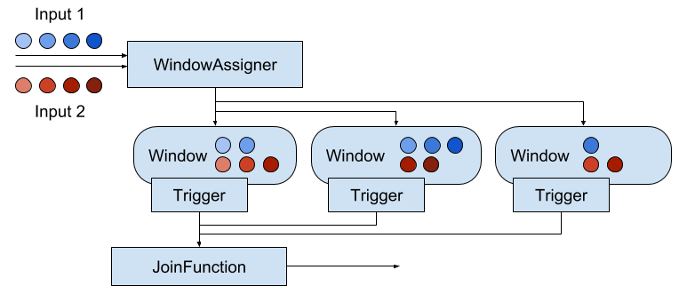
Both input streams are keyed on their key attributes and the common window assigner maps events of both streams to common windows, i.e., a window stores the events of both inputs. When the timer of a window fires, the JoinFunction is called for each combination of elements from the first and the second input, i.e., the cross product. It is also possible to specify a custom trigger and evictor. Since the events of both streams are mapped into the same windows, triggers and evictors behave exactly as in regular window operators.
In addition to joining two streams, it is also possible to co-group two streams on a window by starting the operator definition with coGroup() instead of join(). The overall logic is the same, but instead of calling a JoinFunction for every pair of events from both inputs, a CoGroupFunction is called once per window with iterators over the elements from both inputs.
It should be noted that the joining windowed streams can have unexpected semantics. For instance, assume you join two streams with a join operator that is configured with a one hour tumbling window. An element of the first input will not be joined with an element of the second input even if they are just one second aparat from each other but assigned to two different windows.
In case you cannot express your required join semantics using Flink’s window-based joins, you can implement a lot of custom join logic using a CoProcessFunction. For instance, you can implement an operator that joins all events with timestamps that are not more than a certain time interval apart from each other. Note that you should design such an operator with efficient state access patterns and effective state cleanup strategies.
Flink’s event-time processing is based on the concept of watermarks to reason about the progress in event-time. As discussed before, watermarks are a mechanism to trade off result completeness and result latency. Unless you opt for a very conservative watermark strategy that guarantees to include all relevant records at the cost of high latency, your application will most likely have to handle late elements.
A late element is an element that arrives at an operator when a computation to which it would need to contribute has already been performed. In the context of an event-time window operator an event is late if it arrives at the operator and the window assigner maps it to a window that has already been computed because the operator’s watermark passed the end timestamp of the window.
The DataStream API provides different options for how to handle late events.
In the following, we discuss these options in detail and show how they are applied for process functions and window operators.
The easiest way to handle late events is to simply discard them. Dropping late events is the default behavior for event-time window operators. Hence, a late arriving element will not create a new window.
Process functions can easily filter out late events by comparing their timestamp with the current watermark.
Late events can also be redirected into another DataStream using the side output feature. From there, the late events can be emitted using a regular sink function. Depending on the business requirements, late data can later be integrated into the results of the streaming application with a periodic backfill process.
Example 6-34 shows how to specify a window operator with a side output for late events.
// define an output tag for late sensor readingsvallateReadingsOutput:OutputTag[SensorReading]=newOutputTag[SensorReading]("late-readings")valreadings:DataStream[SensorReading]=???valcountPer10Secs:DataStream[(String,Long,Int)]=readings.keyBy(_.id).timeWindow(Time.seconds(10))// emit late readings to a side output.sideOutputLateData(lateReadingsOutput)// count readings per window.process(newCountFunction())// retrieve the late events from the side output as a streamvallateStream:DataStream[SensorReading]=countPer10Secs.getSideOutput(lateReadingsOutput)
A process function can identify late events by comparing event timestamps with the current watermark and emit them using the regular side output API. Example 6-35 shows a ProcessFunction that filters out late sensor readings from its input and redirects them to a side output stream.
// define a side output tagvallateReadingsOutput:OutputTag[SensorReading]=newOutputTag[SensorReading]("late-readings")// =================== //valreadings:DataStream[SensorReading]=???valfilteredReadings:DataStream[SensorReading]=readings.process(newLateReadingsFilter)// retrieve late readingsvallateReadings:DataStream[SensorReading]=filteredReadings.getSideOutput(lateReadingsOutput)// =================== ///** A ProcessFunction that filters out late sensor readings and* re-directs them to a side output */classLateReadingsFilterextendsProcessFunction[SensorReading,SensorReading]{overridedefprocessElement(r:SensorReading,ctx:ProcessFunction[SensorReading,SensorReading]#Context,out:Collector[SensorReading]):Unit={// compare record timestamp with current watermarkif(r.timestamp<ctx.timerService().currentWatermark()){// this is a late reading => redirect it to the side outputctx.output(lateReadingsOutput,r)}else{out.collect(r)}}}
Late events arrive at an operator after a computation was completed to which they should have contributed. Therefore, the operator emitted a result that is incomplete or inaccurate. Instead of dropping or redirecting late events, another strategy is to recompute an incomplete result and emit an update. However, there are a few issues that need to be taken into account in order to be able to recompute and update results.
An operator that supports recomputing and updating of emitted results needs to preserve all state that is required for the computation after the first result was emitted. However, since it is typically not possible for an operator to retain all state forever, it needs to purge state at some point. Once the state for a certain result was purged the result cannot be updated anymore and late events can only be dropped or redirected.
In addition to keeping state around, the downstream operators or external systems that follow an operator that produces results, which update previously emitted results, need to be able to handle them. For example, a sink operator that writes the results and updates of a keyed window operator to a key-value store could do this by overriding inaccurate results with the latest update using upsert writes. For some use cases it might also be necessary to distinguish between the first result and an update due to a late event.
The window operator API provides a method to explicitly declare that you expect late elements. When using event-time windows, you can specify an additional time period called allowed lateness. A window operator with allowed lateness will not delete a window and its state after the watermark passed the window’s end timestamp. Instead, the operator continues to maintain the complete window for the allowed lateness period. When a late element arrives within the allowed lateness period it is handled like on-time elements and handed to the trigger. When the watermark passes the window end timestamp plus the lateness interval, the window is finally deleted and all subsequent late elements are discarded.
Allowed lateness can be specified using the allowedLateness() method as Example 6-36 demonstrates.
valreadings:DataStream[SensorReading]=???valcountPer10Secs:DataStream[(String,Long,Int,String)]=readings.keyBy(_.id).timeWindow(Time.seconds(10))// process late readings for 5 additional seconds.allowedLateness(Time.seconds(5))// count readings and update results if late readings arrive.process(newUpdatingWindowCountFunction)// =================== ///** A counting WindowProcessFunction that distinguishes between* first results and updates. */classUpdatingWindowCountFunctionextendsProcessWindowFunction[SensorReading,(String,Long,Int,String),String,TimeWindow]{overridedefprocess(id:String,ctx:Context,elements:Iterable[SensorReading],out:Collector[(String,Long,Int,String)]):Unit={// count the number of readingsvalcnt=elements.count(_=>true)// state to check if this is the first evaluation of the window or not.valisUpdate=ctx.windowState.getState(newValueStateDescriptor[Boolean]("isUpdate",Types.of[Boolean]))if(!isUpdate.value()){// first evaluation, emit first resultout.collect((id,ctx.window.getEnd,cnt,"first"))isUpdate.update(true)}else{// not the first evaluation, emit an updateout.collect((id,ctx.window.getEnd,cnt,"update"))}}}
Process functions can also be implemented such that they support late data. Since state management is always custom and manually done in process functions, Flink does not provide a built-in API to support late data. Instead, you can implement the necessary logic using the building blocks of record timestamps, watermarks, and timers.
In this chapter you learned how to implement streaming applications that operate on time. We explained how to configure the time characteristics of a streaming application and how to assign timestamps and watermarks. You learned about time-based operators, including Flink’s process functions, built-in windows, and custom windows. We also discussed the semantics of watermarks, how to trade-off result completeness and result latency, and strategies to handle late events.
1 ListState and its performance characteristics are discussed in detail in Chapter 7.
Stateful operators and user functions are common building blocks of stream processing applications. In fact, most non-trivial operations need to memorize records or partial results because data is streamed and arrives over time1. Many of Flink’s built-in DataStream operators, sources, and sinks are stateful and buffer records or maintain partial results or metadata. For instance, a window operator collects input records for a ProcessWindowFunction or the result of applying a ReduceFunction, a ProcessFunction memorizes scheduled timers, and some sink functions maintain state about transactions to provide exactly-once functionality. In addition to built-in operators and provided sources and sinks, Flink’s DataStream API exposes interfaces to register, maintain, and access state in user-defined functions.
Stateful stream processing has implications on many aspects of a stream processor, such as failure recovery and memory management as well as the maintenance of streaming applications. Chapters 2 and 3 discussed the foundations of stateful stream processing and related details of Flink’s architecture, respectively. Chapter 9 explains how to setup and configure Flink to reliably process stateful applications including configuration of state backends and checkpointing configuration. Chapter 10 gives guidance for how to operate stateful applications, i.e., taking and restoring from application savepoints, rescaling applications, and application upgrades.
This chapter focuses on the implementation of stateful user-defined functions and discusses the performance and robustness of stateful applications. Specifically, we explain how to define and interact with different types of state in user-defined functions. We discuss performance aspects and how to control the size of function state. Finally, we show how to configure keyed state as queryable and how to access it from an external application.
In Chapter 3, we explained that functions can have two types of state, keyed state and operator state. Flink provides multiple interfaces to define stateful functions. In this section, we show how functions with keyed and operator state are implemented.
User functions can employ keyed state to store and access state in the context of a key attribute. For each distinct value of the key attribute, Flink maintains one state instance. The keyed state instances of a function are distributed across all parallel instances of the function, i.e., each parallel instance of the function is responsible for a range of the key domain and maintains the corresponding state instances. Hence, keyed state is very similar to a distributed key-value map. Please consult Chapter 3 for more details on the concepts of keyed state.
Keyed state can only be used by functions which are applied on a KeyedStream. A keyed stream is constructed by calling the DataStream.keyBy(key) method which defines a key on a stream. A KeyedStream is partitioned on the specified key and remembers the key definition. An operator that is applied on a KeyedStream is applied in the context of its key definition.
Flink provides multiple primitives for keyed state. The state primitives define the structure of the state for each individual key. The choice of the right state primitive depends on how the function interacts with the state. The choice also affects the performance of a function because each state backend provides its own implementations for these primitives. The following state primitives are supported by Flink:
ValueState[T]: ValueState[T] holds a single value of type T. The value can be read using ValueState.value() and updated with ValueState.update(value: T).
ListState[T]: ListState[T] holds a list of elements of type T. New elements can be appended to the list by calling ListState.add(value: T) or ListState.addAll(values: java.util.List[T]). The state elements can be accessed by calling ListState.get() which returns an Iterable[T] over all state elements. It is not possible to remove individual elements from ListState, however the list can be updated by calling ListState.update(values: java.util.List[T]).
MapState[K, V]: MapState[K, V] holds a map of keys and values. The state primitive offers many methods of a regular Java Map such as get(key: K), put(key: K, value: V), contains(key: K), remove(key: K), and iterators over the contained entries, keys, and values.
ReducingState[T]: ReducingState[T] offers the same methods as ListState[T] (except for addAll() and update()) but instead of appending values to a list, ReducingState.add(value: T) immediately aggregates value using a ReduceFunction. The iterator returned by get() returns an Iterable with a single entry, which is the reduced value.
AggregatingState[I, O]: AggregatingState[I, O] behaves similar as ReducingState. However, it uses the more general AggregateFunction to aggregate values. AggregatingState.get() computes the final result and returns it as an Iterable with a single element.
All state primitives can be cleared by calling State.clear().
ValueState to compare sensor temperature measurements and raise an alert if the temperature increased significantly between the current and the last measurement.
val sensorData: DataStream[SensorReading]  = ???
// partition and key the stream on the sensor ID
val keyedData: KeyedStream[SensorReading, String] = sensorData
  .keyBy(_.id)


// apply a stateful FlatMapFunction on the keyed stream which
// compares the temperature readings and raises alerts.
val alerts: DataStream[(String, Double, Double)] = keyedSensorData
  .flatMap(new TemperatureAlertFunction(1.1))

// --------------------------------------------------------------

class TemperatureAlertFunction(val threshold: Double)
    extends RichFlatMapFunction[SensorReading, (String, Double, Double)] {

  // the state handle object
  private var lastTempState: ValueState[Double] = _

  override def open(parameters: Configuration): Unit = {
    // create state descriptor
    val lastTempDescriptor =
      new ValueStateDescriptor[Double]("lastTemp", classOf[Double])
    // obtain the state handle
    lastTempState = getRuntimeContext
      .getState[Double](lastTempDescriptor)
  }

  override def flatMap(
      in: SensorReading,
      out: Collector[(String, Double, Double)]): Unit = {
    // fetch the last temperature from state
    val lastTemp = lastTempState.value()
    // check if we need to emit an alert
    if (lastTemp > 0d && (in.temperature / lastTemp) > threshold) {
      // temperature increased by more than the threshold
      out.collect((in.id, in.temperature, lastTemp))
    }
    // update lastTemp state
    this.lastTempState.update(in.temperature)
  }
}
In order to create a state object, we have to register a StateDescriptor with Flink’s runtime via the RuntimeContext which is exposed by a RichFunction (see Chapter 5 for a discussion of the RichFunction interface). The StateDescriptor is specific to the state primitive and includes the name of the state and the data types of the state. The descriptors for ReducingState and AggregatingState also need a ReduceFunction or AggregateFunction object to aggregate the added values. The state name is scoped to the operator such that a function can have more than one state object by registering multiple state descriptors. The data types handled by the state are specified as Class or TypeInformation objects (see Chapter 5 for a discussion of Flink’s type handling). The data type must be specified because Flink needs to create a suitable serializer. Alternatively, it is also possible to explicitly specify a TypeSerializer to control how state is written into a state backend, checkpoint, and savepoint2.
Typically, the state handle object is created in the open() method of the RichFunction. open() is called before any processing methods, such as flatMap() in case of a FlatMapFunction, are called. The state handle object (lastTempState in the example above) is a regular member variable of the function class. Note that the state handle object only provides access to the state but does not hold the state itself.
When a function registers a StateDescriptor, Flink checks if the state backend has data for the function and a state with the given name and type. This might happen if a parallel instance of a stateful function is restarted to recover from a failure or when an application is started from a savepoint. In both cases, Flink links the newly registered state handle object to the existing state. If the state backend does not contain state for the given descriptor, the state that is linked to the handle is initialized as empty.
State can be read and updated in a processing method of a function, such as the flatMap() method of a FlatMapFunction. When the processing method of a function is called with a record, Flink’s runtime automatically puts all keyed state objects of the function into the context of the record’s key as specified by the KeyedStream. Therefore, a function can only access the state which belongs to the record that it currently processes.
The Scala DataStream API offers syntactic shortcuts to define map and flatMap functions with a single ValueState. Example 7-2 shows how to implement the previous example with the shortcut.
val alerts: DataStream[(String, Double, Double)] = keyedSensorData
  .flatMapWithState[(String, Double, Double), Double] {
    case (in: SensorReading, None) =>
      // no previous temperature defined.
      // Just update the last temperature
      (List.empty, Some(in.temperature))
    case (in: SensorReading, lastTemp: Some[Double]) =>
      // compare temperature difference with threshold
      if (lastTemp.get > 0 && (in.temperature / lastTemp.get) > 1.4) {
        // threshold exceeded. Emit an alert and update the last temperature
        (List((in.id, in.temperature, lastTemp.get)), Some(in.temperature))
      } else {
        // threshold not exceeded. Just update the last temperature
        (List.empty, Some(in.temperature))
      }
  }
The flatMapWithState() method expects a function that accepts a Tuple2. The first field of the tuple holds the input record to flatMap, the second field holds an Option of the retrieved state for the key of the processed record. The Option is not defined if the state has not been initialized yet. The function also returns a Tuple2. The first field is a list of the flatMap results, the second field is the new value of the state.Operator state is managed per parallel instance of an operator. All events that are processed in the same parallel subtask of an operator have access to the same state. In Chapter 3, we discussed that Flink supports three types of operator state, list state, list union state, and broadcast state.
A function can work with operator list state by implementing the ListCheckpointed interface. The ListCheckpointed interface does not work with state handles like ValueState or ListState, which are registered at the state backend. Instead, functions implement operator state as regular member variables and interact with the state backend via callback functions of the ListCheckpointed interface. The interface provides two methods:
snapshotState(checkpointId: Long, timestamp: Long): java.util.List[T]
restoreState(java.util.List[T] state): Unit
The snapshotState() method is invoked when Flink requests a checkpoint from the stateful function. The method has two parameters, checkpointId, which is a unique, monotonically increasing identifier for checkpoints, and timestamp, which is the wall clock time when the master initiated the checkpoint. The method has to return the operator state as a list of serializable state objects.
The restoreState() method is always invoked when the state of a function needs to be initialized, i.e., when the job is started (from a savepoint or not) or in case of a failure. The method is called with a list of state objects and has to restore state of the operator based on these objects.
ListCheckpointed interface for a function that counts temperature measurements that exceed a threshold per partition, i.e., for each parallel instance of the operator.
class HighTempCounter(val threshold: Double)
    extends RichFlatMapFunction[SensorReading, (Int, Long)]
    with ListCheckpointed[java.lang.Long] {

  // index of the subtask
  private lazy val subtaskIdx = getRuntimeContext
    .getIndexOfThisSubtask
  // local count variable
  private var highTempCnt = 0L

  override def flatMap(
      in: SensorReading,
      out: Collector[(Int, Long)]): Unit = {
    if (in.temperature > threshold) {
      // increment counter if threshold is exceeded
      highTempCnt += 1
      // emit update with subtask index and counter
      out.collect((subtaskIdx, highTempCnt))
    }
  }

  override def restoreState(
      state: util.List[java.lang.Long]): Unit = {
    highTempCnt = 0
    // restore state by adding all longs of the list
    for (cnt <- state.asScala) {
      highTempCnt += cnt
    }
  }

  override def snapshotState(
      chkpntId: Long,
      ts: Long): java.util.List[java.lang.Long] = {
    // snapshot state as list with a single count
    java.util.Collections.singletonList(highTempCnt)
  }
}
The function in the above example counts per parallel instance how many temperature measurements exceeded a configured threshold . The function uses operator state and has a single state variable for each parallel operator instance that is checkpointed and restored using the methods of the ListCheckpointed interface. Note that the ListCheckpointed interface is implemented in Java and expects java.util.List instead of a Scala native list.
Looking at the example, you might wonder why operator state is handled as a list of state objects. As discussed in Chapter 3, the list structure supports changing the parallelism of functions with operator state. In order to increase or decrease the parallelism of a function with operator state, the operator state needs to be redistributed to a larger or smaller number of task instances. This requires splitting or merging of state objects. Since the logic for splitting and merging of state is custom for every stateful function, this cannot be automatically done for arbitrary types of state.
By providing a list of state objects, functions with operator state can implement this logic in thesnapshotState() and restoreState() methods. The snapshotState() method splits the operator state into multiple parts and the restoreState() method assembles the operator state from possibly multiple parts. When the state of a function is restored, the parts of the state are distributed among all parallel subtasks of the function and handed to the restoreState() method. In case that there are more parallel subtasks than state objects, some subtasks are started with no state, i.e., the restoreState() method is called with an empty list.
Looking again at the example of the HighTempCounter function in Example 7-3, we see that each parallel instance of the operator exposes its state as a list with a single entry. If we would increase the parallelism of this operator, some of the new subtasks would be initialized with an empty state, i.e., start summing from zero. In order to achieve a better state distribution behavior when the HighTempCounter function is rescaled, we can implement the snapshotState() method such that it splits its count into multiple partial counts as shown in Example 7-4.
override def snapshotState(
    chkpntId: Long,
    ts: Long): java.util.List[java.lang.Long] = {
  // split count into ten partial counts
  val div = highTempCnt / 10
  val mod = (highTempCnt % 10).toInt
  // return count as ten parts
  (List.fill(mod)(new java.lang.Long(div + 1)) ++
    List.fill(10 - mod)(new java.lang.Long(div))).asJava
}
A common requirement in streaming applications is to distribute the same information to all parallel instances of a function and maintain it as recoverable state. An example is a stream of rules and a stream of events on which the rules are applied. The operator that applies the rules ingests two input streams, the event stream and the rules stream, and remembers the rules in an operator state in order to apply them to all events of the event stream. Since each parallel instance of the operator must hold all rules in its operator state, the rules stream needs to be broadcasted to ensure that each instance of the operator receives all rules.
In Flink such a state is called broadcast state. Broadcast state can only be combined with a regular DataStream or a KeyedStream. Example 7-5 shows how to implement the temperature alert application with a rules stream to dynamically adjust the alert thresholds.
val keyedSensorData: KeyedStream[SensorReading, String] =
  sensorData.keyBy(_.id)

// the descriptor of the broadcast state
val broadcastStateDescriptor =
  new MapStateDescriptor[String, Double](
    "thresholds",
    classOf[String],
    classOf[Double])

val broadcastThresholds: BroadcastStream[ThresholdUpdate] =
  thresholds.broadcast(broadcastStateDescriptor)

// connect keyed sensor stream and broadcasted rules stream
val alerts: DataStream[(String, Double, Double)] = keyedSensorData
  .connect(broadcastThresholds)
  .process(new UpdatableTempAlertFunction(4.0d))

// --------------------------------------------------------------

class UpdatableTempAlertFunction(val defaultThreshold: Double)
    extends KeyedBroadcastProcessFunction[String, SensorReading, ThresholdUpdate, (String, Double, Double)] {

  // the descriptor of the broadcast state
  private lazy val thresholdStateDescriptor =
    new MapStateDescriptor[String, Double](
      "thresholds",
      classOf[String],
      classOf[Double])

  // the keyed state handle
  private var lastTempState: ValueState[Double] = _

  override def open(parameters: Configuration): Unit = {
    // create keyed state descriptor
    val lastTempDescriptor = new ValueStateDescriptor[Double](
      "lastTemp",
      classOf[Double])

    // obtain the keyed state handle
    lastTempState = getRuntimeContext
      .getState[Double](lastTempDescriptor)
  }

  override def processBroadcastElement(
      update: ThresholdUpdate,
      keyedCtx: KeyedBroadcastProcessFunction[String, SensorReading, ThresholdUpdate, (String, Double, Double)]#KeyedContext,
      out: Collector[(String, Double, Double)]): Unit = {
    // get broadcasted state handle
    val thresholds: MapState[String, Double] = keyedCtx
      .getBroadcastState(thresholdStateDescriptor)

    if (update.threshold >= 1.0d) {
      // configure a new threshold of the sensor
      thresholds.put(update.id, update.threshold)
    } else {
      // remove sensor specific threshold
      thresholds.remove(update.id)
    }
  }

  override def processElement(
      reading: SensorReading,
      keyedReadOnlyCtx: KeyedBroadcastProcessFunction[String, SensorReading, ThresholdUpdate, (String, Double, Double)]#KeyedReadOnlyContext,
      out: Collector[(String, Double, Double)]): Unit = {
    // get read-only broadcast state
    val thresholds: MapState[String, Double] = keyedReadOnlyCtx
      .getBroadcastState(thresholdStateDescriptor)

    // get threshold for sensor
    val sensorThreshold: Double =
      if (thresholds.contains(reading.id)) {
        thresholds.get(reading.id)
      } else {
        defaultThreshold
      }

    // fetch the last temperature from keyed state
    val lastTemp = lastTempState.value()

    // check if we need to emit an alert
    if (lastTemp > 0 &&
         (reading.temperature / lastTemp) > sensorThreshold) {
      // temperature increased by more than the threshold
      out.collect((reading.id, reading.temperature, lastTemp))
    }

    // update lastTemp state
    this.lastTempState.update(reading.temperature)
  }
}
A function with broadcast state is defined in three steps.
You create a BroadcastStream by calling DataStream.broadcast() and provide one or more MapStateDescriptor objects. Each descriptor defines a separate broadcast state of the function that is later applied on the BroadcastStream.
You connect the BroadcastStream with a DataStream or KeyedStream. Note, that the BroadcastStream must be put as an argument in the connect() method.
You apply a function on the connected streams. Depending on whether the other stream was keyed or not, a KeyedBroadcastProcessFunction or BroadcastProcessFunction can be applied.
The BroadcastProcessFunction and KeyedBroadcastProcessFunction differ from a regular CoProcessFunction because the element processing methods are not symmetric. The methods are named processElement() and processBroadcastElement() and called with different context objects. Both context objects offer a method getBroadcastState(MapStateDescriptor) that provides access to a broadcast state handle. However, the broadcast state handle that is returned in the processElement() method provides read-only access to the broadcast state. This is a safety mechanism to ensure that the broadcast state holds the same information in all parallel instances. In addition, both context objects also provide access to the event-time timestamp, the current watermark, the current processing-time, and side outputs, similar to the context objects of a regular ProcessFunction.
The BroadcastProcessFunction and KeyedBroadcastProcessFunction differ from each other as well. The BroadcastProcessFunction does not expose a timer service to register timers and consequently does not offer an onTimer() method. Note that you should not access keyed state from the processBroadcastElement() of the KeyedBroadcastProcessFunction. Since the broadcast input does not specify a key, the state backend cannot access a keyed value and will throw an exception. Instead, the context of the KeyedBroadcastProcessFunction.processBroadcastElement() method provides a method applyToKeyedState(StateDescriptor, KeyedStateFunction) to apply a KeyedStateFunction to the value of each key in the keyed state that is referenced by the StateDescriptor.
The CheckpointedFunction interface is the lowest-level interface to specify stateful functions. It provides hooks to register and maintain keyed state and operator state and is the only interface that gives access to operator list union state, i.e., operator state that is fully replicated in case of a recovery or savepoint restart3.
The CheckpointedFunction interface defines two methods, initializeState() and snapshotState(), which work similarly to the methods of the ListCheckpointed interface for operator list state. The initializeState() method is called when a parallel instance of a CheckpointedFunction is created. This happens when an application is started or when a task is restarted due to a failure. The method is called with a FunctionInitializationContext object which provides access to an OperatorStateStore and an KeyedStateStore object. The state stores are responsible for registering function state with Flink’s runtime and returning the state objects, such as ValueState, ListState, or BroadcastState. Each state is registered with a name that must be unique for the function. When a function registers state, the state store tries to initialize the state by checking if the state backend holds state for the function registered under the given name. If the task was restarted due to a failure or from a savepoint, the state will be initialized from the saved data. If the application was not started from a checkpoint or savepoint, the state will be initially empty.
The snapshotState() method is called immediately before a checkpoint is taken and receives a FunctionSnapshotContext object as parameter. The FunctionSnapshotContext gives access to the unique identifier of the checkpoint and the timestamp when the JobManager initiated the checkpoint. The purpose of the snapshotState() method is to ensure that all state objects are updated before the checkpoint is done. Moreover, in combination with the CheckpointListener interface, the snapshotState() method can be used to consistently write data to external data stores by synchronizing with Flink’s checkpoints.
CheckpointedFunction interface is used to create a function with keyed and operator state that counts per key and operator instance how many sensor readings exceed a specified threshold.
class HighTempCounter(val threshold: Double)
    extends FlatMapFunction[SensorReading, (String, Long, Long)]
    with CheckpointedFunction {

  // local variable for the operator high temperature cnt
  var opHighTempCnt: Long = 0
  var keyedCntState: ValueState[Long] = _
  var opCntState: ListState[Long] = _

  override def flatMap(
      v: SensorReading,
      out: Collector[(String, Long, Long)]): Unit = {
    // check if temperature is high
    if (v.temperature > threshold) {
      // update local operator high temp counter
      opHighTempCnt += 1
      // update keyed high temp counter
      val keyHighTempCnt = keyedCntState.value() + 1
      keyedCntState.update(keyHighTempCnt)
      // emit new counters
      out.collect((v.id, keyHighTempCnt, opHighTempCnt))
    }
  }

  override def initializeState(
      initContext: FunctionInitializationContext): Unit = {
    // initialize keyed state
    val keyCntDescriptor = new ValueStateDescriptor[Long](
      "keyedCnt",
      createTypeInformation[Long])
    keyedCntState = initContext.getKeyedStateStore
      .getState(keyCntDescriptor)

    // initialize operator state
    val opCntDescriptor = new ListStateDescriptor[Long](
      "opCnt",
      createTypeInformation[Long])
    opCntState = initContext.getOperatorStateStore
      .getListState(opCntDescriptor)

    // initialize local variable with state
    opHighTempCnt = opCntState.get().asScala.sum
  }

  override def snapshotState(
      snapshotContext: FunctionSnapshotContext): Unit = {
    // update operator state with local state
    opCntState.clear()
    opCntState.add(opHighTempCnt)
  }
}
Frequent synchronization is a major reason for performance limitations in distributed systems. Flink’s design aims to reduce synchronization points. Checkpoints are implemented based on barriers that flow with the data and therefore avoid global synchronization across all operators of an application.
Due to its checkpointing mechanism, Flink is able to achieve very good performance. However, another implication is that the state of an application is never in a consistent state except for the logical points in time when a checkpoint is taken. For some operators it can be important to know whether a checkpoint completed or not. For example, sink functions that aim write data to external systems with exactly-once guarantees must only emit records that were received before a successful checkpoint to ensure that the received data will not be recomputed in case of a failure.
As discussed in Chapter 3, a checkpoint is only successful if all operator tasks successfully checkpointed their state to the checkpoint storage. Hence, only the JobManager can determine whether a checkpoint is successful or not. Operators that need to be notified about completed checkpoints can implement the CheckpointListener interface. The interface provides the notifyCheckpointComplete(long chkpntId) method, which might be called when the JobManager registers a checkpoint as completed, i.e., when all operators successfully copied their state to the remote storage.
notifyCheckpointComplete() method is called for each completed checkpoint. It is possible that a task misses the notification. This needs to be taken into account when implementing the interface.The way that operators interact with state has implications on the robustness and performance of applications. There are several aspects that affect the behavior of an application such as the choice of the state backend that locally maintains the state and performs checkpoints, the configuration of the checkpointing algorithm, and the size of the application’s state. In this section, we discuss aspects that need to be taken into account in order to ensure robust execution behavior and consistent performance of long-running applications.
In Chapter 3, we explained that Flink maintains operator state of streaming applications in a state backend. The state backend is responsible for storing the local state of each task instance and persisting it to a remote storage when a checkpoint is taken. Because local state can be maintained and checkpointed in different ways, state backends are pluggable, i.e., two applications can use different state backend implementations to maintain their state. Currently, Flink offers three state backends, the InMemoryStateBackend, the FsStateBackend, and the RocksDBStateBackend. Moreover, StateBackend is a public interface such that it is possible to implement custom state backends.
ValueState, ListState, and MapState. The InMemoryStateBackend and the FsStateBackend store state as regular objects on the heap of the TaskManager JVM process. For example, a MapState is backed by a Java HashMap object. While this approach provides very low latencies to read or write state, it has implications on the robustness of an application. If the state of a task instance grows too large, the JVM and all task instances running on it can be killed due to an OutOfMemoryError. Moreover, this approach can suffer from garbage collection pauses because it puts many objects on the heap.
In contrast, the RocksDBStateBackend serializes all state into a RocksDB instance. RocksDB is an embedded key-value store, which persists data to disk. By writing data to disk and supporting incremental checkpoints (see Chapter 3), the RocksDBStateBackend is a good choice for applications with large state. Users reported applications with state sizes of multiple terabytes running on the RocksDBStateBackend. However, reading and writing data to disk and the overhead of de/serializing objects result in lower read and write performance compared to organizing state on the heap. Chapter 3 discussed the differences between Flink’s state backends in more detail.
val env = StreamExecutionEnvironment.getExecutionEnvironment

val checkpointPath: String = ???
val incrementalCheckpoints: Boolean = true
// configure path for checkpoints on the remote filesystem
val backend = new RocksDBStateBackend(
  checkpointPath,
  incrementalCheckpoints)

// configure path for local RocksDB instance on worker
backend.setDbStoragePath(dbPath)
// configure RocksDB options
backend.setOptions(optionsFactory)

// configure state backend
env.setStateBackend(backend)
Please note that the RocksDBStateBackend is an optional module of Flink and not included in Flink’s default classpath. Chapter 5 discusses how to add optional modules to Flink.
Many streaming applications require that failures, such as a failed TaskManager, must not affect the correctness of the computed result. Moreover, application state can be a valuable asset, which must not be lost in case of a failure because it is expensive or impossible to recompute.
In Chapter 3, we explained Flink’s mechanism to create consistent checkpoints of a stateful application, i.e., a snapshot of the state of all built-in and user-defined stateful functions at a point in time when all operators processed all events up to a specific point in the application’s input streams. Flink’s checkpointing technique and the corresponding failure recovery mechanism guarantee exactly-once consistency for state, i.e., the state of an application is same regardless whether failures occurred or not.When an application enables checkpointing, the JobManager initiates checkpoints in regular intervals. The checkpointing interval determines the overhead of the checkpointing mechanism during regular processing and the time it takes to recover from a failure. A shorter checkpointing interval causes higher overhead during regular processing but a faster recovery because less data needs to be reprocessed.
An application enables checkpointing via the StreamExecutionEnvironment shown in Example 7-8.
val env = StreamExecutionEnvironment.getExecutionEnvironment

// set checkpointing interval to 10 seconds (10000 milliseconds)
env.enableCheckpointing(10000L)
Flink provides more tuning knobs to configure the checkpointing behavior, such as the choice of consistency guarantees (exactly-once or at-least-once), the maximum number of checkpoints to preserve, and a timeout to cancel long-running checkpoints. All these options are discussed in detail in Chapter 9.
Stateful streaming applications are often designed to run for a long time but also need to be maintained. For example it might be necessary to fix a bug or to evolve an application by implementing a new feature. In either case, a currently running application needs to be replaced by a new version without losing the state of the application.
Flink supports such updates by taking a savepoint of the running application, stopping it, and starting the new version from the savepoint. However, application updates cannot be supported for arbitrary changes. The original application and its new version need to be savepoint compatible which means that the new version needs to be able to deserialize the data of the savepoint that was taken from the old version and correctly map the data into the state of the its operators.It is important to note that the design of the original version of the application defines if and how the application can be modified in the future. It will not be easy or not even possible to update an application if the original version was not designed with updates in mind. The problem of savepoint compatibility boils down to two issues.
Mapping the individual operator states in a savepoint to the operators of a new application.
Reading the serialized state of the original application with the deserializers of the new version.
When an application is started from a savepoint, Flink associates the state in the savepoint with the operators in the application based on unique identifiers. This matching of state and operators is important, because an updated application might have a different structure, e.g., it might have additional operators or operators have been removed. Each operator has an operator identifier that is serialized into the savepoint along with its state. By default, the identifier is computed as a unique hash based on the operator’s properties and the properties of its predecessors. Hence, the identifier will inevitably change if the operator or its predecessors change and Flink will not be able to map the state of a previous savepoint. The default identifiers are a conservative mechanism to avoid state corruption but prevent many types of application updates. In order to ensure that you can add or remove of operators from your application, you should always manually assign unique identifiers to all of your operators. This is done as shown in Example 7-9.
val alerts: DataStream[(String, Double, Double)] = sensorData
  .keyBy(_.id)
  // apply stateful FlatMap and set unique ID
  .flatMap(new TemperatureAlertFunction(1.1)).uid("alertFunc")
When starting an updated stateful application from a savepoint it might happen that the new version does not require all state that was written into the savepoint because a stateful operator was removed. By default, Flink will not allow to restart an application that does not read all state of a savepoint to prevent state loss. However, it is possible to disable this safety check.
While addressing the problem of matching savepoint state and operators is rather easy to solve by adding unique identifiers, ensuring the compatibility of serializers is more challenging. The best approach here is to configure state serializers for data encodings that support versioning, such as Avro, Protobuf, or Thrift. You should also be aware that serialization compatibility does not only affect state that is explicitly defined in a user-defined function (as discussed in this chapter) but also the internal state of stateful DataStream operators such as window operators or running aggregates. All these functions store intermediate data in state. The type of the state usually depends on the input type of the operator. Consequently, also changing the input and output types of functions affects the savepoint compatibility of an application. Therefore, we also recommend to use data types with encodings that support versioning as input types for built-in DataStream operators with state.An operator with state that is serialized using a versioned encoding can be modified by updating the data type and the schema of its encoding. When the state is read from the savepoint, new fields will be initialized as empty and fields that got dropped will not be read.
If you have already a running application that you need to update but did not use serializers with versioned encodings, Flink offers a migration path for the serialized savepoint data. This functionality is based on two methods in theTypeSerializer interface, snapshotConfiguration() and ensureCompatibility(). Since, serializer compatibility is a fairly advanced and detailed topic, it is not in the scope of this book. We refer you to the documentation of the TypeSerializer interface.The performance of a stateful operator (built-in or user-defined) depends on several aspects, including the data types of the state, the state backend of the application, and the chosen state primitives.
For state backends that de/serialize state objects when reading or writing, such as theRocksDBStateBackend, the choice of the state primitive (ValueState, ListState, or MapState) can have a major impact on the performance of an application. For instance, ValueState is completely deserialized when it is accessed and serialized when it is updated. The ListState implementation of the RocksDBStateBackend deserializes all list entries before constructing the Iterable to read the values. However, adding a single value to the ListState, i.e., appending it to the end of the list, is a cheap operation because only the appended value is serialized. The MapState of the RocksDBStateBackend allows to read and write values per key, i.e., only those keys and values are de/serialized that are read or written. When iterating over the entry set of a MapState, the serialized entries are pre-fetched from RocksDB and only deserialized when a key or value is actually accessed.
For example, with the RocksDBStateBackend it is more efficient to use MapState[X, Y] instead of ValueState[HashMap[X, Y]]. ListState[X] has an advantage over ValueState[List[X]] if elements are frequently appended to the list and the elements of the list are less frequently accessed.
Streaming applications are often designed to run continuously for months or years. If the state of an application is continuously increasing, it will at some point grow too large and kill the application unless action is taken to scale the application to more resources. In order to prevent increasing resource consumption of an application over time, it is important that the size of operator state is controlled. Since the handling of state directly affects the semantics of an operator, Flink cannot automatically clean up state and free storage. Instead, all stateful operators must control the size of their state and have to ensure that it is not infinitely growing.
A common reason for growing state is keyed state on an evolving key domain. In this scenario, a stateful function receives records with keys that are only active for a certain period of time and are never received after that. A typical example is a stream of click events where clicks have a session id attribute that expires after some time. In such a case, a function with keyed state would accumulate state for more and more keys. As the key space evolves, the state of expired keys becomes stale and useless. A solution for this problem is to remove the state of expired keys. However, a function with keyed state can only access the state of a key if it received a record with that key. In many cases, a function does not know if a record will be the last one for a key. Hence, it will not be able to evict the state for the key because it might receive another record for the key.This problem does not only exist for custom stateful functions but also for some of the built-in operators of the DataStream API. For example, computing running aggregates on a KeyedStream, either with the build-in aggregations functions such as min, max, sum, minBy, or maxBy or with a custom ReduceFunction or AggregateFunction, keeps the state for each key and never discards it. Consequently, these functions should only be used if the key values are from a constant and bounded domain. Other examples are windows with count-based triggers, which process and clean their state when a certain number of records has been received. Windows with time-based triggers (both, processing time and event time) are not affected by this because they trigger and purge their state based on time.
This means that you should take application requirements and the properties of its input data, such as key domain, into account when designing and implementing stateful operators. If your application requires keyed state for a moving key domain, it should ensure that the state of keys is cleared when it is not needed anymore. This can be done by registering timers for a point of time in the future4. Similar to state, timers are registered in the context of the currently active key. When the timer fires, a callback method is called and the context of timer’s key is loaded. Hence, the callback method has full access to the key’s state and can also clear it. There are currently two functions that offer support to register timers, the Trigger interface for windows and the ProcessFunction. Both have been introduced in Chapter 6.
ProcessFunction that compares two subsequent temperature measurements and raises an alert if the difference is greater than a threshold. This is the same use case as in the keyed state example before, but the ProcessFunction also clears the state for keys (i.e., sensors) that have not provided any new temperature measurement within one hour of event-time.
class StateCleaningTemperatureAlertFunction(val threshold: Double)
    extends ProcessFunction[SensorReading, (String, Double, Double)] {

  // the keyed state handle for the last temperature
  private var lastTempState: ValueState[Double] = _
  // the keyed state handle for the last registered timer
  private var lastTimerState: ValueState[Long] = _

  override def open(parameters: Configuration): Unit = {
    // register state for last temperature
    val lastTempDescriptor =
      new ValueStateDescriptor[Double]("lastTemp", classOf[Double])
    lastTempState = getRuntimeContext
      .getState[Double](lastTempDescriptor)

    // register state for last timer
    val timerDescriptor: ValueStateDescriptor[Long] =
      new ValueStateDescriptor[Long]("timerState", classOf[Long])
    lastTimerState = getRuntimeContext
      .getState(timerDescriptor)
  }

  override def processElement(
      in: SensorReading,
      ctx: ProcessFunction[SensorReading, (String, Double, Double)]#Context,
      out: Collector[(String, Double, Double)]) = {
    // get current watermark and add one hour
    val checkTimestamp =
      ctx.timerService().currentWatermark() + (3600 * 1000)
    // register new timer.
    // Only one timer per timestamp will be registered.
    ctx.timerService().registerEventTimeTimer(checkTimestamp)
    // update timestamp of last timer
    lastTimerState.update(checkTimestamp)

    // fetch the last temperature from state
    val lastTemp = lastTempState.value()
    // check if we need to emit an alert
    if (lastTemp > 0.0d && (in.temperature / lastTemp) > threshold) {
      // temperature increased by more than the threshold
      out.collect((in.id, in.temperature, lastTemp))
    }

    // update lastTemp state
    this.lastTempState.update(in.temperature)
  }

  override def onTimer(
      ts: Long,
      ctx: ProcessFunction[SensorReading, (String, Double, Double)]#OnTimerContext,
      out: Collector[(String, Double, Double)]): Unit = {
    // get timestamp of last registered timer
    val lastTimer = lastTimerState.value()

    // check if the last registered timer fired
    if (lastTimer != null.asInstanceOf[Long] && lastTimer == ts) {
      // clear all state for the key
      lastTempState.clear()
      lastTimerState.clear()
    }
  }
}
The state-cleaning mechanism implemented by the above ProcessFunction works as follows. For each input event, the processElement() method is called. Before comparing the temperature measurements and updating the last temperature, the method registers a clean-up timer. The clean-up time is computed by reading the timestamp of the current watermark and adding one hour. The timestamp of the latest registered timer is held in an additional ValueState[Long] named lastTimerState. After that, the method compares the temperatures, possibly emits an alert, and updates its state.
While being executed, a ProcessFunction maintains a list of all registered timers, i.e., registering a new timer does not override previously registered timers5. As soon as the internal event-time clock of the operator (driven by the watermarks) exceeds the timestamp of a registered timer, the onTimer() method is called. The method validates if the fired timer was the last registered timer by comparing the timestamp of the fired timer with the timestamp held in the lastTimerState. If this is the case, the method removes all managed state, i.e., the last temperature and the last timer state.
Many stream processing applications need to share their results with other applications. A common pattern is to write results into a database or key-value store and other applications retrieve the result from that data store. Such an architecture implies that a separate system needs to be setup and maintained which can be a major effort, especially if this needs to be a distributed system as well.
Apache Flink features queryable state to address use cases that usually would require an external data store to share data. In Flink, any keyed state can be exposed to external applications as queryable state and act as a read-only key-value store. The stateful streaming application processes events as usual and stores and updates its intermediate or final results in an queryable state. External applications request the state for each key while the streaming application is running. Note that only key-point-queries are supported. It is not possible to request key ranges or even run more complex queries.
Queryable state does not address all use cases that require an external data store. For example, the queryable state is only accessible while the application is running. It is not accessible while the application is restarted due to an error, for rescaling the application, or to migrate it to another cluster. However, it makes many other applications much easier to realize, such as real-time dashboards or other monitoring applications.
In the following, we will discuss the architecture of Flink’s queryable state service and explain how streaming applications can expose queryable state and external applications can query it.
Flink’s queryable state service consists of three processes.
The QueryableStateClient is used by an external application to submit queries and retrieve results.
The QueryableStateClientProxy accepts and serves client requests. Each TaskManager runs a client proxy. Since keyed state is distributed across all parallel instances of an operator, the proxy needs to identify the TaskManager that maintains the state for the requested key. This information is requested from the JobManager, which manages the key group assignment6, and cached. The client proxy retrieves the state from the state server of the respective TaskManager and serves the result to the client.
The QueryableStateServer serves the requests of a client proxy. Each TaskManager runs a state server which fetches the state of a queried key from the local state backend and returns it to the requesting client proxy.
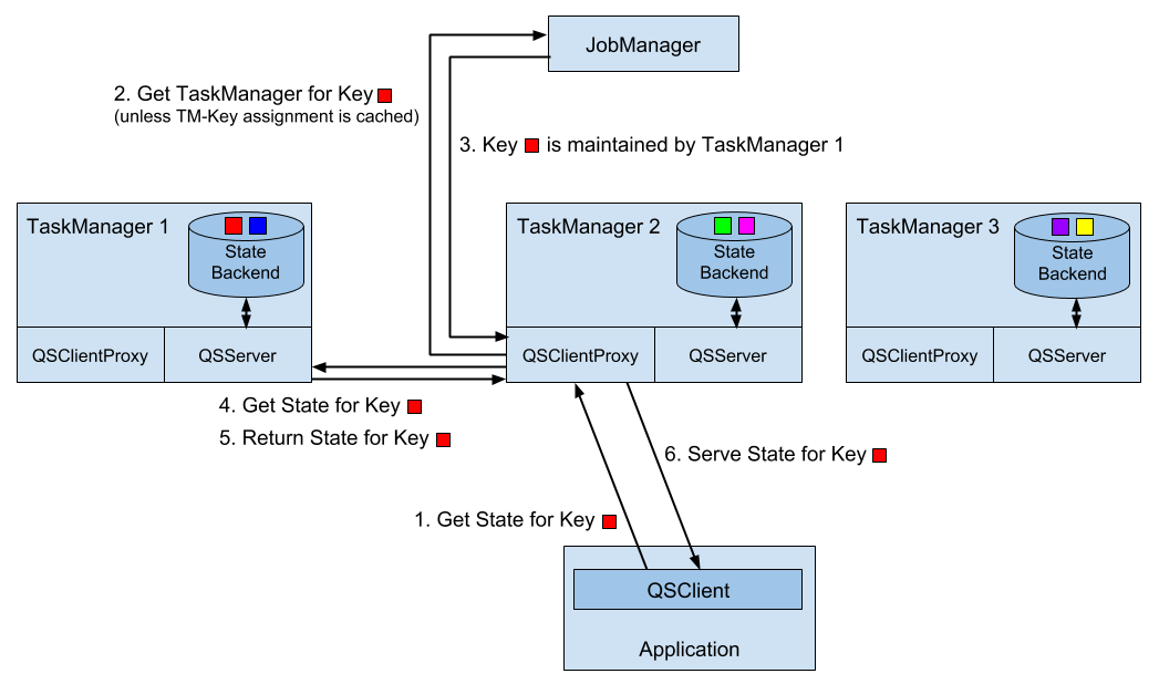
In order to enable the queryable state service in a Flink setup, i.e., to start client proxy and server threads within the TaskManagers, you need to add the flink-queryable-state-runtime JAR file to the classpath of the TaskManager process. This is done by copying it from the ./opt folder of you installation into the ./lib folder. When the JAR file is in the classpath, the queryable state threads are automatically started and can serve requests of the queryable state client. When properly configured, you will find the following log message in the TaskManager logs.
Started the Queryable State Proxy Server @ …
The ports used by the client proxy and server and additional parameters can be configured in the ./conf/flink-conf.yaml file.
Implementing a streaming application with queryable state is easy. All you have to do is to define a function with keyed state and enable the state as queryable by calling the setQueryable(String) method on the StateDescriptor before obtaining the state handle. Example 7-11 shows how to make the lastTempState queryable that we used in the example to illustrate the usage of the keyed state.
 override def open(parameters: Configuration): Unit = {

  // create state descriptor
  val lastTempDescriptor =
    new ValueStateDescriptor[Double]("lastTemp", classOf[Double])
  // enable queryable state and set its external identifier
  lastTempDescriptor.setQueryable("lastTemperature")
  // obtain the state handle
  lastTempState = getRuntimeContext
    .getState[Double](lastTempDescriptor)
}
The external identifier that is passed with the setQueryable() method can be freely chosen and is only used to configure the queryable state client.
In addition to the generic way of enabling queries on any type of keyed state, Flink also offers shortcuts to define stream sinks that store the events of a stream in queryable state. Example 7-12 shows how to use a queryable state sink.
val tenSecsMaxTemps: DataStream[(String, Double)] = sensorData
  // project to sensor id and temperature
  .map(r => (r.id, r.temperature))
  // compute every 10 seconds the max temperature per sensor
  .keyBy(_._1)
  .timeWindow(Time.seconds(10))
  .max(1)

// store max temperature of the last 10 secs for each sensor
// in a queryable state.
tenSecsMaxTemps
  // key by sensor id
  .keyBy(_._1)
  .asQueryableState("maxTemperature")
The asQueryableState() method appends a queryable state sink to the stream. The type of the queryable state is a ValueState that holds values of the type of the input stream, i.e., in case of our example (String, Double). For each received record, the queryable state sink upserts the record into the ValueState, such that always the latest event per key is stored. The asQueryableState() method is overloaded with two more methods.
asQueryableState(id: String, stateDescriptor: ValueStateDescriptor[T]) can be used to configure the ValueState in more detail, e.g., to configure a custom serializer.
asQueryableState(id: String, stateDescriptor: ReducingStateDescriptor[T]) configures a ReducingState instead of a ValueState. The ReducingState is also updated for each incoming record. However, in contrast to the ValueState, the new record does not replace the existing value but is instead combined with the previous version using the state’s ReduceFunction.
An application with a function that has queryable state is executed just like any other application. You only have to ensure that the TaskManagers are configured to start their queryable state services as discussed in the previous section.
Any JVM-based application can query queryable state of a running Flink application by using the QueryableStateClient. This class is provided by the flink-queryable-state-client-java dependency, that you can add to your project as follows.
<dependency>
  <groupid>org.apache.flink</groupid>
  <artifactid>flink-queryable-state-client-java_2.11</artifactid>
  <version>1.5.0</version>
</dependency>
The QueryableStateClient is initialized with the hostname of any TaskManager and the port on which the queryable state client proxy is listening. By default, the client proxy listens on port 9067 but the port can be configured in the ./conf/flink-conf.yaml file.
val client: QueryableStateClient =
  new QueryableStateClient(tmHostname, proxyPort)
Once you obtained a state client, you can query the state of an application by calling the getKvState() method. The method takes several parameters, such as the JobID of the running application, the state identifier, the key for which the state should be fetched, the TypeInformation for the key, and the StateDescriptor of the queried state. The JobID can be obtained via the REST API, the web UI, or the log files. The getKvState() method returns a CompletableFuture[S] where S is the type of the state, e.g., ValueState[_] or MapState[_, _]. Hence, the client can send out multiple asynchronous queries and wait for their results.
object TemperatureDashboard {

  // assume local setup and TM runs on same machine as client
  val proxyHost = "127.0.0.1"
  val proxyPort = 9069

  // jobId of running QueryableStateJob.
  // can be looked up in logs of running job or the web UI
  val jobId = "d2447b1a5e0d952c372064c886d2220a"

  // how many sensors to query
  val numSensors = 5
  // how often to query the state
  val refreshInterval = 10000

  def main(args: Array[String]): Unit = {
    // configure client with host and port of queryable state proxy
    val client = new QueryableStateClient(proxyHost, proxyPort)

    val futures = new Array[
      CompletableFuture[ValueState[(String, Double)]]](numSensors)
    val results = new Array[Double](numSensors)

    // print header line of dashboard table
    val header =
      (for (i <- 0 until numSensors) yield "sensor_" + (i + 1))
        .mkString("\t| ")
    println(header)

    // loop forever
    while (true) {
      // send out async queries
      for (i <- 0 until numSensors) {
        futures(i) = queryState("sensor_" + (i + 1), client)
      }
      // wait for results
      for (i <- 0 until numSensors) {
        results(i) = futures(i).get().value()._2
      }
      // print result
      val line = results.map(t => f"$t%1.3f").mkString("\t| ")
      println(line)

      // wait to send out next queries
      Thread.sleep(refreshInterval)
    }
    client.shutdownAndWait()
  }

  def queryState(
      key: String,
      client: QueryableStateClient)
    : CompletableFuture[ValueState[(String, Double)]] = {

    client
      .getKvState[String, ValueState[(String, Double)], (String, Double)](
        JobID.fromHexString(jobId),
        "maxTemperature",
        key,
        Types.STRING,
        new ValueStateDescriptor[(String, Double)](
          "", // state name not relevant here
          createTypeInformation[(String, Double)]))
  }
}
In order to run the example, you have to start the streaming application with the queryable state first. Once it is running, look for the JobID in the log file or the web UI, set the JobID in the code of the dashboard and run it as well. The dashboard will then start querying the state of the running streaming application.
Basically every non-trivial streaming application is stateful. The DataStream API provides powerful yet easy-to-use tooling to access and maintain operator state. It offers different types of state primitives and supports pluggable state backends. While developers have lots of flexibility to interact with state, Flink’s runtime manages Terabytes of state and ensures exactly-once semantics in case of failures. The combination of time-based computations as discussed in Chapter 6 and scalable state management, empowers developers to realize sophisticated streaming applications. Queryable state is an easy-to-use feature and can save you the effort of setting up and maintaining a database or key-value store to expose the results of a streaming application to external applications.
1 This differs from batch processing where user-defined functions, such as a GroupReduceFunction, are called when all data to be processed has been collected.
2 The serialization format of state is an important aspect when updating an application and discussed later in this chapter.
3 See Chapter 3 for details on how operator list union state is distributed.
4 Timers can be based on event-time or processing-time.
5 Timers with identical timestamps are deduplicated. That is also the reason why we compute the clean-up time based on the watermark and not on the record timestamp.
6 Key Groups are discussed in Chapter 3.
Data can be stored in many different systems, such as file systems, object stores, relational database systems, key-value stores, search indexes, event logs, and message queues, and so on. Each class of systems has been designed for specific access patterns and excels at serving a certain purpose. Consequently, today’s data infrastructures often consist of many different storage systems. Before adding a new component into the mix, a natural question to ask is “How well does it work with the other components in my stack?”
Adding a data processing system, such as Apache Flink, requires careful considerations because it does not include its own storage layer but relies on external storage systems to ingest and persist data. Hence, it is important for data processors like Flink to provide a well-equipped library of connectors to read data from and write data to external systems as well as an API to implement custom connectors. However, just being able to read or write data to external data stores is not sufficient for a stream processor that wants to provide meaningful consistency guarantees in case of failures.
In this chapter, we discuss how source and sink connectors affect the consistency guarantees of Flink streaming applications and present Flink’s most popular connectors to read and write data. You will learn how to implement custom source and sink connectors and how to implement functions that send asynchronous read or write requests to external data stores.
In Chapter 3, you learned that Flink’s checkpointing and recovery mechanism periodically takes consistent checkpoints of an application’s state. In case of a failure, the state of the application is restored from the latest completed checkpoint and processing continues. However, being able to reset the state of an application to a consistent point is not sufficient to achieve satisfying processing guarantees for an application. Instead, the source and sink connectors of an application need to be integrated with Flink’s checkpointing and recovery mechanism and provide certain properties to be able to give meaningful guarantees.
In order to provide exactly-once state consistency for an application1, each source connector of the application needs to be able to be reset to a previously checkpointed read position. When taking a checkpoint, a source operator persists its reading positions and restores these positions during recovery. Examples for source connectors that support the checkpointing of reading positions are file-based sources that store the reading offset in the byte stream of the file or a Kafka source that stores the reading offsets in the topic partitions it consumes. If an application ingests data from a source connector that is not able to store and reset a reading position, it might suffer from data loss in case of a failure and only provide at-most-once guarantees.
The combination of Flink’s checkpointing and recovery mechanism and resettable source connectors guarantees that an application will not lose any data. However, the application might emit results twice because all results that have been emitted after the last successful checkpoint (the one to which the application falls back in case of a recovery) will be emitted again. Therefore, resettable sources and Flink’s recovery mechanism, are not sufficient to provide end-to-end exactly-once guarantees even though the application state is exactly-once consistent.
An application that aims to provide end-to-end exactly-once guarantees requires special sink connectors. There are two techniques that sink connectors can apply in different situations to achieve exactly-once guarantees, idempotent writes and transactional writes.
An idempotent operation can be performed several times but will only result in a single change. For example, repeatedly inserting the same key-value pair into a hashmap is an idempotent operation because the first insert operation adds the value for the key into the map and all following insertions will not change the map since it already contains the key-value pair. On the other hand, an append operation is not an idempotent operation, because appending an element multiple times results in multiple appends. Idempotent write operations are interesting for streaming applications because they can be performed multiple times without changing the result. Hence, they can to some extend mitigate the effect of replayed results as caused by Flink’s checkpointing mechanism.
It should be noted an application that relies on idempotent sinks to achieve exactly-once results must guarantee that it overrides previously written results while it replays. For example, an application with a sink that upserts into a key-value store must ensure that it deterministically computes the keys that are used to upsert. Moreover, applications that read from the sink system might observe unexpected results during the time when an application recovers. When the replay starts, previously emitted results might be overridden by earlier results. Hence, an application that consumes the output of the recovering application might witness a jump back in time, e.g., read a smaller count than before. Also, the overall result of the streaming application will be in an inconsistent state while the replay is in progress because some results will be overridden but others not yet. Once the replay completes and the application is past the point at which it previously failed, the result will be consistent again.
The second approach to achieve end-to-end exactly-once consistency is based on transactional writes. The idea here is to only write those results to an external sink system that have been computed before the last successful checkpoint. This behavior guarantees end-to-end exactly-once because in case of a failure, the application is reset to the last checkpoint and no results have been emitted to the sink system after that checkpoint. By only writing data once a checkpoint is completed, the transactional approach does not suffer from the replay inconsistency of the idempotent writes. However, it adds latency because results only become visible when a checkpoint completes.
Flink provides two building blocks to implement transactional sink connectors, a generic Write-Ahead-Log (WAL) sink and a Two-Phase-Commit (2PC) sink. The WAL sink writes all result records into application state and emits them to the sink system once it received the notification that a checkpoint was completed. Since the sink buffers records in the state backend, the WAL sink can be used with any kind of sink system. However, it cannot provide bulletproof exactly-once guarantees2, adds to the state size of an application, and the sink system has to deal with a spikey writing pattern.
In contrast, the 2PC sink requires a sink system that offers transactional support or exposes building blocks to emulate transactions. For each checkpoint, the sink starts a transaction and appends all received records to the transaction, i.e., writing them to the sink system without committing them. When it receives the notification that a checkpoint completed, it commits the transaction and materializes the written results. The mechanism relies on the ability of a sink to commit a transaction after recovering from a failure that was opened before a completed checkpoint.
The 2PC protocol piggybacks on Flink’s existing checkpointing mechanism. The checkpoint barriers are notifications to start a new transaction, the notifications of all operators about the success of their individual checkpoint are their commit votes, and the messages of the JobManager that notify about the success of a checkpoint are the instructions to commit the transactions. In contrast to WAL sinks, 2PC sinks can achieve exactly-once output depending on the sink system and the sink’s implementation. Moreover, a 2PC sink continuously writes records to the sink system compared to the spiky writing pattern of a WAL sink.
Table 8-0 shows the end-to-end consistency guarantees for different types of source and sink connectors that can be achieved in the best case, i.e., depending on the implementation of the sink, the actual consistency might be worse.
| Non-resettable source | Resettable source | |
| Any sink | At-most-once | At-least-once |
| Idempotent sink | At-most-once | Exactly-once* (temporary inconsistencies during recovery) |
| WAL sink | At-most-once | At-least-once |
| 2PC sink | At-most-once | Exactly-once |
Apache Flink provides connectors to read data from and write data to a variety of different storage systems. Message queues and event logs, such as Apache Kafka, Kinesis, or RabbitMQ, are common sources to ingest data streams. In batch processing dominated environments, data streams are also often ingested by monitoring a file system directory and reading files as they appear.
On the sink side, data streams are often produced into message queues to make the events available to subsequent streaming applications, written to file systems for archiving or making the data available for offline analytics or batch applications, or inserted into key-value stores or relational database systems, like Cassandra, ElasticSearch, or MySQL, to make the data searchable and queryable, or to serve dashboard applications.
Unfortunately, there are no standard interfaces for most of these storage systems, except JDBC for relational DBMS. Instead, every system features its own connector library with a proprietary protocol. As a consequence, processing systems like Flink need several dedicated connectors to be able to read events from and write events to the most commonly used message queues, event logs, file systems, key-value stores, and database systems.
Flink provides connectors for Apache Kafka, Kinesis, RabbitMQ, Apache Nifi, various file systems, Cassandra, ElasticSearch, and JDBC. In addition, the Apache Bahir project provides additional Flink connectors for ActiveMQ, Akka, Flume, Netty, and Redis.
In order to use provided connectors in your application, you need to add their dependencies to the build file of your project. We explained how to add connector dependencies in Chapter 5.
In the following, we discuss the connectors for Apache Kafka, file-based sources and sinks, and Apache Cassandra. These are the most widely used connectors and they also represent important types of source and sink systems. You can find more information about the other connectors in Apache Flink’s or Apache Bahir’s documentation.
Apache Kafka is a distributed streaming platform. Its core is a distributed publish-subscribe messaging system that is widely adopted to ingest and distribute event streams. We briefly explain the main concepts of Kafka before we dive into the details of Flink’s Kafka connector.
Kafka organizes event streams as so-called topics. A topic is an event log, which guarantees that events are read in the same order in which they were written. In order to scale writing to and reading from a topic, it can be split into partitions which are distributed across a cluster. The ordering guarantee is limited to a partition, i.e., Kafka does not provide ordering guarantees when reading from different partitions. The reading position in a Kafka partition is called an offset.
Flink provides source connectors for Kafka versions from 0.8.x to 1.1.x (the latest version as of this writing). Until Kafka 0.11.x, the API of the client library evolved and new features were added. For instance, Kafka 0.10.0 added support for record timestamps. Since release 1.0.x, the API remained stable such that Flink’s connector for Kafka 0.11.x works as well for Kafka 1.0.x and 1.1.x. The dependency for the Flink Kafka 0.11 connector is added to a Maven project as shown in Example 8-1.
<dependency>
   <groupId>org.apache.flink</groupId>
   <artifactId>flink-connector-kafka-0.11_2.11</artifactId>
   <version>1.5.0</version>
</dependency>
A Flink Kafka connector ingests an event stream in parallel. Each parallel instance of the source operator may read from multiple partitions or no partition if the number of partitions is less than the number of source instances. A source instance tracks for each partition its current reading offset and includes it into its checkpoint data. When recovering from a failure, the offsets are restored and the source instance continues reading from the checkpointed offset. The Flink Kafka connector does not rely on Kafka’s own offset tracking mechanism which is based on so-called consumer groups. Figure 8-1 shows the assignment of partitions to source instances.
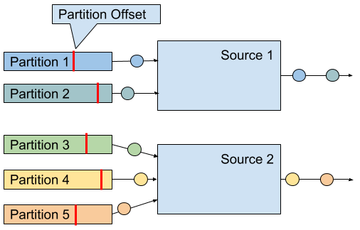
A Kafka 0.11.x source connector is created as shown in Example 8-2.
val properties = new Properties()
properties.setProperty("bootstrap.servers", "localhost:9092")
properties.setProperty("group.id", "test")

val stream: DataStream[String] = env.addSource(
 new FlinkKafkaConsumer011[String](
   "topic",
   new SimpleStringSchema(),
   properties))
The constructor takes three arguments. First argument defines the topics to read from. This can be a single topic, a list of topics, or a regular expression pattern that matches all topics to read from. When reading from multiple topics, the Kafka connector treats all partitions of all topics the same and multiplexes their events into a single stream.
The second argument is a DeserializationSchema or KeyedDeserializationSchema. Kafka messages are stored as raw byte messages and need to be deserialized into Java or Scala objects. The SimpleStringSchema, which is used in Example 8-2, is a built-in DeserializationSchema that simply deserializes a byte array into a String. In addition, Flink provides implementations for Apache Avro and String-based JSON encodings. DeserializationSchema and KeyedDeserializationSchema are public interfaces such that you can always implement custom deserialization logic.
The third parameter is a Properties object that configures the Kafka client which is internally used to connect to and read from Kafka. A minimum Properties configuration consists of two entries, "bootstrap.servers" and "group.id". The Kafka 0.8 connector needs in addition the "zookeeper.connect" property. Please consult the Kafka documentation for additional configuration properties.
In order to extract event-time timestamps and generate watermarks, you can provide an AssignerWithPeriodicWatermarks or AssignerWithPunctuatedWatermarks to a Kafka consumer by calling FlinkKafkaConsumer011.assignTimestampsAndWatermarks() 3. An assigner is applied to each partition to leverage the per partition ordering guarantees and the source instance merges the partition watermarks according to the watermark propagation protocol (see Chapter 3). Note that the watermarks of a source instance cannot make progress if a partition becomes inactive and does not provide messages. As a consequence, a single inactive partition can stall a whole application because the application’s watermarks do not make progress.
Since version 0.10.0, Kafka supports message timestamps. When reading from Kafka version 0.10 or later, the consumer will automatically extract the message timestamp as event-time timestamp if the application runs in event-time mode. In this case, you still need to generate watermarks and should apply a AssignerWithPeriodicWatermarks or AssignerWithPunctuatedWatermarks that forwards the previously assigned Kafka timestamp.
There are a few more configuration options that we would like to briefly mention. It is possible to configure the starting position from which the partitions of a topic are initially read. Valid options are listed below.
The last reading position as known by Kafka for the consumer group that was configured via the “group.id” parameter. This is the default behavior:
FlinkKafkaConsumer011.setStartFromGroupOffsets()
The earliest offset of each individual partition:
FlinkKafkaConsumer011.setStartFromEarliest()
The latest offset of each individual partition:
FlinkKafkaConsumer011.setStartFromLatest()
All records with a timestamp greater than a given timestamp (requires Kafka 0.10.x or later):
FlinkKafkaConsumer011.setStartFromTimestamp()
Specific reading positions for all partitions as provided by a Map object:
FlinkKafkaConsumer011.setStartFromSpecificOffsets()
Note that this configuration only affects the first reading positions. In case of a recovery or when starting from a savepoint, an application will start reading from the offsets that are stored in the checkpoint or savepoint.
A Flink Kafka consumer can be configured to automatically discover new partitions that were added to a topic or topics that match a regular expression. These features are disabled by default and can be enabled by adding the parameter flink.partition-discovery.interval-millis with a non-negative value to the Properties object.
Flink provides sink connectors for Kafka versions from 0.8.x to 1.1.x (the latest version as of this writing). Until Kafka 0.11.x, the API of the client library evolved and new features were added, such as record timestamp support with Kafka 0.10.0 and transactional writes with Kafka 0.11.0 Since release 1.0.x, the API remained stable such that Flink’s connector for Kafka 0.11.x works as well for Kafka 1.0.x and 1.1.x. The dependency for the Flink Kafka 0.11 connector is added to a Maven project as shown in Example 8-3.
<dependency>
   <groupId>org.apache.flink</groupId>
   <artifactId>flink-connector-kafka-0.11_2.11</artifactId>
   <version>1.5.0</version>
</dependency>
A Kafka sink is added to a DataStream application as shown in Example 8-4.
val stream: DataStream[String] = ...

val myProducer = new FlinkKafkaProducer011[String](
       "localhost:9092",         // broker list
       "topic",                  // target topic
       new SimpleStringSchema)   // serialization schema

stream.addSink(myProducer)
The constructor, which is used in Example 8-4, receives three parameters. The first parameter is a comma-separated String of Kafka broker addresses. The second parameter is the name of the topic to which the data is written and the last parameter is a SerializationSchema that converts the input types of the sink (String in Example 8-4) into a byte array. A SerializationSchema is the counterpart of the DeserializationSchema that we discussed in the Kafka source section.
The different Flink Kafka producer classes provide more constructors with different combinations of arguments. The following arguments can be provided.
Similar to the Kafka source connector, you can pass a Properties object to pass custom options to the internal Kafka client. When using Properties, the list of brokers has to be provided as "bootstrap.servers" property. Please have a look at the Kafka documentation for a comprehensive list of parameters.
You can specify a FlinkKafkaPartitioner to control how records are mapped to Kafka partitions. We will discuss this feature in more depth later in this section.
Instead of using a SerializationSchema to convert records into byte arrays, you can also specify a KeyedSerializationSchema, which serializes a record into two byte arrays, one for the key and one for the value of a Kafka message. Moreover, KeyedSerializationSchema also exposes more Kafka specific functionality, such as overriding the target topic to write to multiple topics.
The consistency guarantees that Flink’s Kafka sink can provide depend on the version of the Kafka cluster into which the sink produces. For Kafka 0.8.x, the Kafka sink does not provide any guarantees, i.e., records might be written zero, one, or multiple times.
For Kafka 0.9.x and 0.10.x, Flink’s Kafka sink can provide at-least-once guarantees for an application, if the following aspects are correctly configured.
Flink’s checkpointing is enabled and all sources of the application are resettable.
The sink connector throws an exception if a write does not succeed, causing the application to fail and recover. This is the default behavior. The internal Kafka client can be configured to retry writes before declaring them as failed by setting the retries property to a value larger than 0 (which is the default). You can also configure the sink to only log write failures by calling setLogFailuresOnly(true) on the sink object. Note that this will void any output guarantees of the application.
The sink connector waits for Kafka to acknowledge in-flight records before completing its checkpoint. This is the default behavior. By calling setFlushOnCheckpoint(false) on the sink object, you can disable this waiting. However, this will also disable any output guarantees.
Kafka 0.11.x introduced support for transactional writes. Due to this feature, Flink’s Kafka sink is also able to provide exactly-once output guarantees given that the sink and Kafka are properly configured. Again, a Flink application must enable checkpointing and consume from resettable sources. Moreover, the FlinkKafkaProducer011 provides a constructor with a Semantic parameter, which controls the consistency guarantees provided by the sink. Possible values are
Semantic.NONE, which provides no guarantees, i.e., records might be lost or written multiple times.
Semantic.AT_LEAST_ONCE, which guarantees that no write is lost but it might be duplicated. This is the default setting.
Semantic.EXACTLY_ONCE, which builds on Kafka’s transactions to write each record exactly once.
There are a few things to consider, when running a Flink application with a Kafka sink that operates in exactly-once mode and it helps to roughly understand how Kafka processes transactions. In a nutshell, Kafka’s transactions work by appending all messages to the log of a partition and marking messages of open transactions as uncommitted. Once a transaction is committed, the markers are changed to committed. A consumer that reads from a topic can be configured with an isolation level (via the isolation.level property) to declare whether it can read uncommitted messages (read_uncommitted, the default) or not (read_committed). If the consumer is configured to read_committed, it stops consuming from a partition once it encounters an uncommitted message. Hence, open transactions can block consumers from reading a partition and introduce significant delays. Kafka guards against this effect by rejecting and closing transactions after a timeout interval, which is configured with the transaction.timeout.ms property.
In the context of Flink’s Kafka sink, this is important, because transactions that time out, for example due to too long recovery cycles, lead to data loss. Hence, it is crucial to configure the transaction timeout property appropriately. By default, the Flink Kafka sink sets transaction.timeout.ms to one hour, which means that you probably need to adjust the transaction.max.timeout.ms property of your Kafka setup, which is set to 15 minutes by default. Moreover, the visibility of committed messages depends on the checkpoint interval of a Flink application. Please refer to the Flink documentation to learn about a few other corner cases when enabling exactly-once consistency.
The default configuration of a Kafka cluster can still lead to data loss, even after a write was acknowledged. You should carefully revise the configuration of your Kafka setup, paying special attention to the following parameters:
acks
log.flush.interval.messages
log.flush.interval.ms
log.flush.*
We refer you to the Kafka documentation for details about its configuration parameters and guidelines for a suitable configuration.
When writing messages to a Kafka topic, a Flink Kafka sink task can choose to which partition of the topic to write to. A FlinkKafkaPartitioner can be defined in some constructors of the Flink Kafka sink. If not specified, the default partitioner maps each sink task to a single Kafka partition, i.e., all records that are emitted by the same sink task are written to the same partition and a single partition may contain the records of multiple sink tasks if there are more tasks than partitions. If the number of partitions is larger than the number of subtasks, the default configuration results in empty partitions which can cause problems for applications consuming the topic in event-time mode.
By providing a custom FlinkKafkaPartitioner, you can control how records are routed to topic partitions. For example, you can create a partitioner that is based on a key attribute of the records or a round-robin partitioner for even distribution. There is also the option to let Kafka partition the messages based on the message key. This requires to provide a KeyedSerializationSchema in order to extract the message keys and configure the FlinkKafkaPartitioner parameter with null to disable the default partitioner.
Finally, Flink’s Kafka sink can be configured to write message timestamps as supported since Kafka 0.10.0. Write the event-time timestamp of a record to Kafka is enabled by calling setWriteTimestampToKafka(true) on the sink object.
File systems are commonly used to store large amount of data in a cost efficient way. In big data architectures they often serve as data source and data sink for batch processing applications. In combination with advanced file formats, such as Apache Parquet or Apache ORC, file systems can efficiently serve analytical query engines such as Apache Hive, Apache Impala, or Presto. Therefore, file systems are commonly used to “connect” streaming and batch applications.
Apache Flink features a resettable source connector to read streams from files. The file system source is part of the flink-streaming-java module. Hence, you do not need to add any other dependency to use this feature. Flink supports different types of file systems, such as local file system (including locally mounted NFS or SAN shares, Hadoop HDFS, Amazon S3, and OpenStack Swift FS). Please refer to Chapter 9 to learn how to configure file systems in Flink.
val lineReader = new TextInputFormat(null)

val lineStream: DataStream[String] = env.readFile[String](
  lineReader,                 // The FileInputFormat
  "hdfs:///path/to/my/data",  // The path to read
  FileProcessingMode
    .PROCESS_CONTINUOUSLY,    // The processing mode
  30000L)                     // The monitoring interval in ms
The arguments of the StreamExecutionEnvironment.readFile() method are
A FileInputFormat that is responsible for reading the content of the files. We discuss the details of this interface in more detail later in this section. The null parameter of TextInputFormat the example in Example 8-5, defines the path which is separately set.
The path that should be read. If the path refers to a file, the single file is read. If the path refers to a directory, the FileInputFormat scans the directory for files to read.
The mode in which the path should be read. The mode can either be PROCESS_ONCE or PROCESS_CONTINUOUSLY. In PROCESS_ONCE mode, the read path is scanned once when the job is started and all matching files are read. In PROCESS_CONTINUOUSLY, the path is periodically scanned (after an initial scan) and new files are continuously read.
The interval in which the path is periodically scanned in milliseconds. The parameter is ignored in PROCESS_ONCE mode.
A FileInputFormat is a specialized InputFormat to read files from a file system4. A FileInputFormat reads files in two steps. First it scans a file system path and creates so-called input splits for all matching files. An input split defines a range on a file, typically via a start offset and a length. After dividing a large file into multiple splits, the splits can be distributed to multiple reader tasks to read the file in parallel. Depending on the encoding of a file, it can be necessary to only generate a single split to read the file as a whole. The second step of a FileInputFormat is to receive an input split, read the file region that is defined by the split, and return all corresponding records.
A FileInputFormat that is used in a DataStream application should also implement the CheckpointableInputFormat interface, which defines methods to checkpoint and reset the the current reading position of an InputFormat within a file split. The file system source connector provides only at-least-once guarantees when checkpointing is enabled if the FileInputFormat does not implement the CheckpointableInputFormat interface because the input format will start reading from the beginning of the split that was processed when the last complete checkpoint was taken.
In version 1.5.0, Flink provides three FileInputFormat types that implement CheckpointableInputFormat. TextInputFormat reads text files line-wise (split by newline characters), subclasses of CsvInputFormat read files with comma-separated values, and AvroInputFormat reads files with Avro encoded records.
In PROCESS_CONTINUOUSLY mode, the file system source connector identifies new files based on their modification timestamp. This means that a file is completely reprocessed if it is modified, which includes appending writes. Therefore, a common technique to continuously ingest files is to write them in a temporary directory and atomically moving them to the monitored directory once they are finalized. When a file was completely ingested and a checkpoint completed, it can be removed from the directory. Monitoring ingested files by tracking the modification timestamp also has implications if you read from file stores with eventually-consistent list operations, such as S3. Since files might not appear in order of their modification timestamps, they may be ignored by the file system source connector.
Note that in PROCESS_ONCE mode, no checkpoints are taken after the file system path was scanned and all splits were created.
If you want to use a file system source connector in an event-time application, you should be aware that it can be challenging to generate watermarks due to the mechanism that distributes generated input splits. Input splits are generated in a single process and round-robin distributed to all parallel readers which process them in order of the modification timestamp of the referenced file and file name. In order to generate satisfying watermarks you need to reason about the smallest timestamp of a record that is included in a split which is later processed by the task.
Writing a stream into files is a common requirement, for example to prepare data with low-latency for offline ad-hoc analysis. Since most applications can only read files once they are finalized and streaming applications run for long periods of time, streaming sink connectors typically chunk their output into multiple files. Moreover, it is common that records are organized into so-called buckets, such that consuming applications have more control which data to read.
In contrast to the file system source connector, the Flink sink connector is not contained in the flink-streaming-java module and needs to be added by declaring a dependency in your build file. Example 8-6 shows the corresponding entry in a Maven pom.xml file.
<dependency>
  <groupId>org.apache.flink</groupId>
  <artifactId>flink-connector-filesystem_2.11</artifactId>
  <version>1.5.0</version>
</dependency>
Flink’s file system sink connector provides end-to-end exactly-once guarantees for an application given that the application is configured with exactly-once checkpoints and all its sources are reseted in case of a failure. We will discuss the recovery mechanism in more detail later in this section.
Flink’s file system sink connector is called BucketingSink. Example 8-7 shows how to create a BucketingSink with minimal configuration and append it to a stream.
val input: DataStream[String] = …
val fileSink = new BucketingSink[String]("/base/path")

input.addSink(fileSink)
When the BucketingSink receives a record, the record is assigned to a bucket. A bucket is a subdirectory of the base path that is configured in the constructor of the BucketingSink, i.e., "/base/path" in Example 8-7. The bucket is chosen by a Bucketer, which is a public interface and returns the path to the directory to which the record will be written. The Bucketer is configured with the BucketingSink.setBucketer() method. If no Bucketer is explicitly specified, a DateTimeBucketer is used that creates hourly buckets based on the processing time when a record is written.
Each bucket directory contains multiple part files that can be concurrently written by multiple parallel instances of the BucketingSink. Moreover, each parallel instance chunks its output into multiple part files. The path of a part file has the following format
[base-path]/[bucket-path]/[part-prefix]-[task-no]-[task-file-count]
For example given a base path of "/johndoe/demo" and a part prefix of "part", the path "/johndoe/demo/2018-07-22--17/part-4-8" points to the 8th file that was written by the 5th (0-indexed) sink task to bucket "2018-07-22--17", i.e., the 5pm bucket of July 22nd, 2018.
A task creates a new part file, when the current file exceeds a size threshold (default is 384 MB) or if no record was appended for a certain period of time (default is one minute). Both thresholds can be configured with the methods BucketingSink.setBucketSize() and BucketingSink.setInactiveBucketThreshold().
Records are written to a part file using a Writer. The default writer is the StringWriter, which calls the toString() method of a record and writes records newline separated into the part file. A custom Writer can be configured with the BucketingSink.setWriter() method. Flink provides writers that produce Hadoop sequence files (SequenceFileWriter) or Hadoop Avro Key/Value files (AvroKeyValueSinkWriter).
The BucketingSink provides exactly-once output guarantees. The sink achieves this by a commit protocol that moves files through different stages, in-progress, pending, and finished, and which is based on Flink’s checkpointing mechanism. While a sink writes to a file, the file is in the in-progress state. Once a file reaches the size limit or its inactivity threshold is exceeded, it is closed and moved into the pending state by renaming it. Pending files are moved into the finished state (again by renaming) when the next checkpoint completes. The BucketingSink provides setter methods to configure prefixes and suffixes for files in the different stages, i.e., in-progress, pending, finished.
In case of a failure, a sink task needs to reset its current in-progress file to its writing offset at the last successful checkpoint. This can be done in two ways. Typically, the sink task closes the current in-progress file and removes the invalid tail of a file with the file system’s truncate operation. However, if the file system does not support truncating a file (such as older versions of HDFS), the sink task closes the current in-progress file and writes a valid-length file, that contains the valid length of the oversized in-progress file. An application that reads files produced by a BucketingSink on a file system that does not support truncate, must respect the valid-length file to ensure that each output record is only read once.
Note that the BucketingSink will never move files from pending into finished state if checkpointing is not enabled. If you would like to use the sink without consistency guarantees, you can set the prefix and suffix for pending files to an empty string.
We would like to point out that the BucketingSink in Flink 1.5.0 has a few limitations. First, it is restricted to file systems which are directly supported by Hadoop’s FileSystem abstraction. Second, the Writer interface is not able to support batched output formats such as Apache Parquet and Apache ORC. Both limitations are on the roadmap to be fixed in a future Flink version.
Apache Cassandra is a popular, scalable, and highly available column store database system. Cassandra models data sets as tables of rows that consist of multiple typed columns. One or more columns have to be defined as (composite) primary key. Each row can be uniquely identified by its primary key. Among other APIs, Cassandra features the Cassandra Query Language (CQL), a SQL-like language to read and write records and create, modify, and delete database objects, such as keyspaces and tables.
Flink provides a sink connector to write data streams to Cassandra. Cassandra’s data model is based on primary keys and all writes to Cassandra happen with upsert semantics. In combination with exactly-once checkpointing, resettable sources, and deterministic application logic, upsert writes yield eventually exactly-once output consistency. The output is only eventually consistent, because results are reset to a previous version during recovery, i.e., consumers might read older results than they had read before. Also the versions of values for multiple keys might be out of sync.
In order to prevent temporal inconsistencies during recovery and provide exactly-once output guarantees also for applications with non-deterministic application logic, Flink’s Cassandra connector can be configured to leverage a write-ahead log. We will discuss the write-ahead log mode in more detail later in this section.
Example 8-8 shows the dependency that you need to add to the build file of your application in order to use the Cassandra sink connector.<dependency> <groupId>org.apache.flink</groupId> <artifactId>flink-connector-cassandra_2.11</artifactId> <version>1.5.0</version> </dependency>
To illustrate the usage of the Cassandra sink connector, we use the simple example of a Cassandra table that holds data about sensor readings and consists of two columns, sensorId and temperature. The CQL statements in Example 8-9 create a keyspace “example” and a table “sensors” in that keyspace.
CREATE KEYSPACE IF NOT EXISTS example
 WITH replication = {'class': 'SimpleStrategy', 'replication_factor': '1'};

CREATE TABLE IF NOT EXISTS example.sensors (
 sensorId VARCHAR,
 temperature FLOAT,
 PRIMARY KEY(name)
);
Flink provides different sink implementations to write data streams of different data types to Cassandra. Flink’s Java tuples and Row type, Scala’s built-in tuples and case classes are handled differently than user-defined Pojo types. We discuss both cases separately.
Example 8-10 shows how to create a sink that writes a DataStream of tuple, case class, or row types into a Cassandra table. In this example, aDataStream[(String, Float)] is written into the “sensors” table.
val readings: DataStream[(String, Float)] = ???

val sinkBuilder: CassandraSinkBuilder[(String, Float)] =
 CassandraSink.addSink(readings)
sinkBuilder
 .setHost("localhost")
 .setQuery(
   "INSERT INTO example.sensors(sensorId, temperature) VALUES (?, ?);")
 .build()
Cassandra sinks are created and configured using a builder that is obtained by calling the CassandraSink.addSink() method with the DataStream object that should be emitted. The method returns a builder which corresponds to the data type of the DataStream. In Example 8-10, it returns a builder for a Cassandra sink that handles Scala tuples.
The Cassandra sink builders for tuples, case classes, and rows require the specification of a CQL INSERT query5. The query is configured using the CassandraSinkBuilder.setQuery() method. During execution, the sink registers the query as prepared statement and converts the fields of tuples, case classes, or rows into parameters for the prepared statement. The fields are mapped to the parameters based on their position, i.e., the first value is converted into the first parameter and so on.
Since Pojo fields do not have a natural order, Pojos need to be treated differently. Example 8-11 shows how to configure a Cassandra sink for a Pojo of type SensorReading.
val readings: DataStream[SensorReading] = ???

CassandraSink.addSink(readings)
 .setHost("localhost")
 .build()
As you can see in Example 8-11, we do not specify an INSERT query. Instead, Pojos are handed to Cassandra’s Object Mapper which automatically maps Pojo fields to fields of a Cassandra table. In order for this to work, the Pojo class and its fields need to be annotated with Cassandra annotations and provide setters and getters for all fields as shown in Example 8-12. The default constructor is required by Flink as mentioned in Chapter 5 when discussing supported data types.
@Table(keyspace = "example", name = "sensors")
class SensorReadings(
 @Column(name = "sensorId") var id: String,
 @Column(name = "temperature") var temp: Float) {

 def this() = {
    this("", 0.0)
 }

 def setId(id: String): Unit = this.id = id
 def getId: String = id
 def setTemp(temp: Float): Unit = this.temp = temp
 def getTemp: Float = temp
}
In addition to configuration options of the examples in Example 8-10 and Example 8-11, a Cassandra sink builder provides a few more methods to configure the sink connector.
setClusterBuilder(ClusterBuilder): The ClusterBuilder builds a Cassandra Cluster which manages the connection to Cassandra. Among other options, it can configure the hostnames and ports of one or more contact points, define load balancing, retry, and reconnection policies, and provide access credentials.
setHost(String, [Int]): This method is a shortcut for a simple ClusterBuilder that is configured with the hostname and port of a single contact point. If no port is configured, Cassandra’s default port 9042 is used.
setQuery(String): Specifies the CQL INSERT query to write tuples, case classes, or rows to Cassandra. A query must not be configured to emit Pojos.
setMapperOptions(MapperOptions): Provides options for Cassandra’s object mapper, such as configurations for consistency, TTL, null field handling. The options are ignored if the sink emits tuples, case classes, or rows.
enableWriteAheadLog([CheckpointCommitter]): Enables the write-ahead log to provide exactly-once output guarantees in case of non-deterministic application logic. The CheckpointCommitter is used to store information about completed checkpoints in an external data store. If no CheckpointCommitter is configured, the information is written into a specific Cassandra table.
The Cassandra sink connector with write-ahead log is implemented based on Flink’s GenericWriteAheadSink operator. How this operator works, including the role of the CheckpointCommitter, and which consistency guarantees it provides is described in more detail in a dedicated section later in this chapter.
The DataStream API provides two interfaces to implement source connectors along with corresponding RichFunction abstract classes:
SourceFunction and RichSourceFunction can be used to define non-parallel source connectors, i.e., sources that run with a single task.ParallelSourceFunction and RichParallelSourceFunction can be used to define source connectors that run with multiple parallel task instances.Besides their difference in being non-parallel and parallel, both interfaces are identical. Just like the rich variants of processing functions6, subclasses of RichSourceFunction and RichParallelSourceFunction can override the open() and close() methods and access a RuntimeContext that provides the number of parallel task instances and the index of the current instance, among other things.
SourceFunction and ParallelSourceFunction define two methods:
void run(SourceContext<T> ctx)void cancel()The run() method is doing the actual work of reading or receiving records and ingesting them into a Flink application. Depending on the system from which the data is received, the data might be pushed or pulled. The run() method is just called once by Flink and runs in a dedicated source thread, typically reading or receiving data and emits records in an endless loop (infinite stream). The task can be explicitly canceled at some point in time or terminate in case of a finite stream when the input is fully consumed.
The cancel() method is invoked by Flink when the application is cancelled and shut down. In order to perform a graceful shutdown, the run() method, which runs in a separate thread, should terminate as soon as the cancel() method was called.
Example 8-13 shows a simple source function that counts from 0 to Long.MaxValue.
class CountSource extends SourceFunction[Long] {
  var isRunning: Boolean = true

  override def run(ctx: SourceFunction.SourceContext[Long]) = {

    var cnt: Long = -1
    while (isRunning && cnt < Long.MaxValue) {
      cnt += 1
      ctx.collect(cnt)
    }
  }

  override def cancel() = isRunning = false
}
Earlier in this chapter, we explained that Flink can only provide satisfying consistency guarantees for applications that use source connectors which are able to replay their output data. A source function can replay its output if the external system that provides the data exposes an API to retrieve and reset a reading offset. Examples for such systems are filesystems that provide the offset of a file stream and a seek method to move a file stream to a specific position or Apache Kafka, which provides offsets for each partition of a topic and can set the reading position of a partition. A counterexample is a source connector that reads data from a network socket, which immediately discards delivered data.
A source function that supports output replay needs to be integrated with Flink’s checkpointing mechanism and must persist all current reading positions when a checkpoint is taken. When the application is started or recovers from a failure, the reading offsets are retrieved from the latest checkpoint or savepoint. If the application is started without existing state, the reading offsets should be set to a default value. A resettable source function needs to implement the CheckpointedFunction interface and should store the reading offsets and all related meta information, such as file paths or partition ids, in operator list state or operator union list state depending on how the offsets should be distributed to parallel task instances in case of a rescaled application. See Chapter 3 for details on the distribution behavior of operator list state and union list state.
In addition, it is important to ensure that the SourceFunction.run() method, which runs in a separate thread, does not advance the reading offset and emit data, while a checkpoint is taken, i.e., while the CheckpointedFunction.snapshotState() method is called. This is done by guarding the code in run() that advances the reading position and emits records in a block that synchronizing on a lock object, which is obtained from the SourceContext.getCheckpointLock() method.
CountSource of Example 8-13 to be resettable.
class ResettableCountSource
    extends SourceFunction[Long] with CheckpointedFunction {

  var isRunning: Boolean = true
  var cnt: Long = _
  var offsetState: ListState[Long] = _

  override def run(ctx: SourceFunction.SourceContext[Long]) = {
    while (isRunning && cnt < Long.MaxValue) {
      // synchronize data emission and checkpoints
      ctx.getCheckpointLock.synchronized {
        cnt += 1
        ctx.collect(cnt)
      }
    }
  }

  override def cancel() = isRunning = false

  override def snapshotState(snapshotCtx: FunctionSnapshotContext): Unit = {
    // remove previous cnt
    offsetState.clear()
    // add current cnt
    offsetState.add(cnt)
  }

  override def initializeState(
      initCtx: FunctionInitializationContext): Unit = {

    val desc = new ListStateDescriptor[Long]("offset", classOf[Long])
    offsetState = initCtx.getOperatorStateStore.getListState(desc)
    // initialize cnt variable
    val it = offsetState.get()
    cnt = if (null == it || !it.iterator().hasNext) {
      -1L
    } else {
      it.iterator().next()
    }
  }
}
Another important aspect of source functions are timestamps and watermarks. As pointed out in Chapters 3 and 6, the DataStream API provides two options to assign timestamps and generate watermarks. Timestamps and watermarks can be assigned and generate by a dedicated TimestampAssigner (see Chapter 6 for details) or be assigned and generated by a source function.
A source function assigns timestamps and emits watermarks through its SourceContext object. The SourceContext provides the following methods:
def collectWithTimestamp(T record, long timestamp): Unitdef emitWatermark(Watermark watermark): UnitcollectWithWatermark() emits a record with its associated timestamp and emitWatermark() emits the provided watermark.
Besides removing the need for an additional operator, assigning timestamps and generating watermarks in a source function can be beneficial if one parallel instance of a source function consumes records from multiple stream partitions, such as partitions of a Kafka topic. Typically, external systems, such as Kafka, only guarantee message order within a stream partition. Given the case of a source function operator that runs with a parallelism of two and which reads data from a Kafka topic with six partitions, each parallel instance of the source function will read records from three Kafka topic partitions. Consequently, each instance of the source function multiplexes the records of three stream partitions to emit them. Multiplexing records most likely introduces additional out-of-orderness with respect to the event-time timestamps such that a downstream timestamp assigner might produce more late records than expected.
To avoid such behavior, a source function can generate watermarks for each stream partition independently and always emit the smallest watermark of each partition as its watermark. This way, it can ensure that the order guarantees on each partition is leveraged and no unnecessary late records are emitted.
Another problem that source functions have to deal with are instances that become idle and do not emit any more data. This can be very problematic, because it may prevent the whole application from advancing its watermarks and hence lead to a stalling application. Since watermarks should be data driven, a watermark generator (either being integrated in a source function or in a timestamp assigner) will not emit new watermarks if it does not receive input records. If you look at how Flink propagates and updates watermarks (see Chapter 3), you can see that a single operator that does not advance watermarks can put all watermarks of an application to an halt if the application involves a shuffle operation (keyBy(), rebalance(), etc.).
Flink provides a mechanism to avoid such situations by marking source functions as temporarily idle. While being idle, Flink’s watermark propagation mechanism will ignore the idle stream partition. The source is automatically set as active as soon as it starts to emit records again. A source function can decide on its own when it marks itself as idle and does so by calling the method SourceContext.markAsTemporarilyIdle().
In Flink’s DataStream API, any operator or function can send data to an external system or application. It is not required that a DataStream eventually flows into a sink operator. For instance, you could implement a FlatMapFunction that emits each incoming record via an HTTP POST call and not via its Collector. Nonetheless, the DataStream API provides a dedicated SinkFunction interface and a corresponding RichSinkFunction abstract class7.
The SinkFunction interface provides a single method:
void invoke(IN value, Context ctx)The Context object of the SinkFunction provides access to the current processing time, the current watermark, i.e., the current event time at the sink, and the timestamp of the record.
Example 8-15 shows the example of a simple SinkFunction that writes sensor readings to a socket. Note that you need to start a process that listens on the socket before starting the program. Otherwise, the program fails with a ConnectException because a connection to the socket could not be opened. On Linux you can run the command nc -l localhost 9191 to listen on port localhost:9191.
val readings: DataStream[SensorReading] = ???

// write the sensor readings to a socket
readings.addSink(new SimpleSocketSink("localhost", 9191))
  // set parallelism to 1 because only one thread can write to a socket
  .setParallelism(1)

// -----

class SimpleSocketSink(val host: String, val port: Int)
    extends RichSinkFunction[SensorReading] {

  var socket: Socket = _
  var writer: PrintStream = _

  override def open(config: Configuration): Unit = {
    // open socket and writer
    socket = new Socket(InetAddress.getByName(host), port)
    writer = new PrintStream(socket.getOutputStream)
  }

  override def invoke(
      value: SensorReading,
      ctx: SinkFunction.Context[_]): Unit = {
    // write sensor reading to socket
    writer.println(value.toString)
    writer.flush()
  }

  override def close(): Unit = {
    // close writer and socket
    writer.close()
    socket.close()
  }
}
As discussed previously in this chapter, the end-to-end consistency guarantees of an application depend on the properties of its sink connectors. In order to achieve end-to-end exactly-once semantics, an application requires either idempotent or transactional sink connectors. The SinkFunction in Example 8-15 does neither perform idempotent writes nor feature transactional writes. Due to the append-only characteristic of a socket, it is not possible to perform idempotent writes. Since a socket does not have built-in transactional support, transactional writes could only be done using Flink’s generic Write-Ahead-Log (WAL) sink. In the following sections, you will learn how to implement idempotent or transactional sink connectors.
For many applications, the SinkFunction interface is sufficient to implement an idempotent sink connector. Whether this is possible depends on 1) the result data of the application and 2) the external sink system.
The example shown in Example 8-16 illustrates how to implement and use an idempotent SinkFunction that writes to a JDBC database, in this case an embedded Apache Derby database.
val readings: DataStream[SensorReading] = ???

// write the sensor readings to a Derby table
readings.addSink(new DerbyUpsertSink)

// -----

class DerbyUpsertSink extends RichSinkFunction[SensorReading] {
  var conn: Connection = _
  var insertStmt: PreparedStatement = _
  var updateStmt: PreparedStatement = _

  override def open(parameters: Configuration): Unit = {
    // connect to embedded in-memory Derby
    conn = DriverManager.getConnection(
       "jdbc:derby:memory:flinkExample",
       new Properties())
    // prepare insert and update statements
    insertStmt = conn.prepareStatement(
      "INSERT INTO Temperatures (sensor, temp) VALUES (?, ?)")
    updateStmt = conn.prepareStatement(
      "UPDATE Temperatures SET temp = ? WHERE sensor = ?")
  }

  override def invoke(r: SensorReading, context: Context[_]): Unit = {
    // set parameters for update statement and execute it
    updateStmt.setDouble(1, r.temperature)
    updateStmt.setString(2, r.id)
    updateStmt.execute()
    // execute insert statement if update statement did not update any row
    if (updateStmt.getUpdateCount == 0) {
      // set parameters for insert statement
      insertStmt.setString(1, r.id)
      insertStmt.setDouble(2, r.temperature)
      // execute insert statement
      insertStmt.execute()
    }
  }

  override def close(): Unit = {
    insertStmt.close()
    updateStmt.close()
    conn.close()
  }
}
Since Apache Derby does not provide a built-in UPSERT statement, the example sink performs UPSERT writes by first trying to update a row and inserting a new row if no row with the given key exists. The Cassandra sink connector follows the same approach when the write-ahead log is not enabled.
Whenever an idempotent sink connector is not suitable, either due to the characteristics of the application’s output, the properties of the required sink system, or due to stricter consistency requirements, transactional sink connectors can be an alternative. As described before, transactional sink connectors need to be integrated with Flink’s checkpointing mechanism because they may only commit data to the external system when a checkpoint completed successfully.
In order to ease the implementation of transactional sinks, Flink’s DataStream API provides two templates that can be extended to implement custom sink operators. Both templates implement the CheckpointListener interface to receive notifications from the JobManager about completed checkpoints (see Chapter 7 for details about the interface).
The GenericWriteAheadSink collects all outgoing records per checkpoint and stores them in the operator state of the sink task. The state is checkpointed and recovered in case of a failure. When a task receives a checkpoint completion notification, it writes the records of the completed checkpoints to the external system. The Cassandra sink connector with enabled write-ahead log implements this interface.
The TwoPhaseCommitSinkFunction leverages transactional features of the external sink system. For every checkpoint, it starts a new transaction and writes all following records to the sink system in the context the current transaction. The sink commits a transaction when it receives the completion notification of the corresponding checkpoint.
In the following, we describe both interfaces and their consistency guarantees in more detail.
The GenericWriteAheadSink eases the implementation of sink operators with improved consistency properties. The operator is integrated with Flink checkpointing mechanism and aims to write each record exactly-once to an external system. However, you should be aware that failure scenarios exist in which a write-ahead log sink emits records more than once. Hence, the GenericWriteAheadSink does not provide bulletproof exactly-once guarantees but only at-least-once guarantees. We will discuss these scenarios in more detail later in this section.
GenericWriteAheadSink works be appending all received records to a write-ahead log that is segmented by checkpoints. Everytime the sink operator receives a checkpoint barrier, it starts a new section and all following records are appended to the new section. The write-ahead log is stored and checkpointed as operator state. Since the log will be recovered, no records will be lost in case of a failure.
When the GenericWriteAheadSink receives a notification about a completed checkpoint, it emit all records that are stored in the write-ahead log in the segment corresponding to the successful checkpoint. Depending on the concrete implementation of the sink operator, the records can be written to any kind of storage or message system. When all records have been successfully emitted, the corresponding checkpoint must be internally committed.
A checkpoint is committed in two steps. First, the sink persistently stores the information that the checkpoint was committed and secondly it removes the records from the write-ahead log. It is not possible to store the commit information in Flink’s application state because it is not persistent and would be reset in case of a failure. Instead, the GenericWriteAheadSink relies on a pluggable component called CheckpointCommitter to store and lookup information about committed checkpoints in an external persistent storage. For example, the Cassandra sink connector by default uses a CheckpointCommitter that writes to Cassandra.
Thanks to the built-in logic of GenericWriteAheadSink, it is not difficult to implement a sink that leverages a write-ahead log. Operators that extend GenericWriteAheadSink need to provide three constructor parameters:
CheckpointCommitter as discussed before,TypeSerializer to serialize the input records, andCheckpointCommitter to identify commit information across application restarts.Moreover, the write-ahead operator needs to implement a single method.
boolean sendValues(Iterable<IN> values, long chkpntId, long timestamp)
The GenericWriteAheadSink calls the sendValues() method to write the records of a completed checkpoint to the external storage system. The method receives an Iterable over all records of a checkpoint, the id of the checkpoint, and the timestamp of when the checkpoint was taken. The method must return true if all writes succeeded and false if a write failed.
FileCheckpointCommitter that we do not discuss here. You can look up its implementation in the repository that contains the examples of the book.
Note that the GenericWriteAheadSink does not implement the SinkFunction interface. Therefore, sinks that extend GenericWriteAheadSink cannot be added using DataStream.addSink() but are attached using the DataStream.transform() method.
val readings: DataStream[SensorReading] = ???

// write the sensor readings to the standard out via a write-ahead log
readings.transform(
  "WriteAheadSink", new SocketWriteAheadSink)

// -----

class StdOutWriteAheadSink extends GenericWriteAheadSink[SensorReading](
    // CheckpointCommitter that commits checkpoints to the local file system
    new FileCheckpointCommitter(System.getProperty("java.io.tmpdir")),
    // Serializer for records
    createTypeInformation[SensorReading]
      .createSerializer(new ExecutionConfig),
    // Random JobID used by the CheckpointCommitter
    UUID.randomUUID.toString) {

  override def sendValues(
      readings: Iterable[SensorReading],
      checkpointId: Long,
      timestamp: Long): Boolean = {

    for (r <- readings.asScala) {
      // write record to standard out
      println(r)
    }
    true
  }
}
The examples repository contains an application that fails and recovers in regular intervals to demonstrate the behavior of the StdOutWriteAheadSink and a regular DataStream.print() sink in case of failures.
We have mentioned before, that the GenericWriteAheadSink cannot provide bulletproof exactly-once guarantees for all that are built with it. There are two failure cases that can result in records being emitted more than once.
The program fails while a task is current running the sendValues() method. If the external sink system cannot atomically write multiple records, i.e., either all or none, some records might have been written and others not. Since the checkpoint was not committed yet, the sink will write all records again during recovery.
All records are correctly written and the sendValues() method returns with true, however, the program fails before the CheckpointCommitter is called or the CheckpointCommitter fails to commit the checkpoint. During recovery, all records of not yet committed checkpoints will be written again.
Please note, that these discussed failure scenarios do not affect the exactly-once guarantees of the Cassandra sink connector because it performs UPSERT writes. The Cassandra sink connector benefits from the write-ahead log because it guards from non-deterministically keys and prevents inconsistent writes to Cassandra.
Flink provides the TwoPhaseCommitSinkFunction interface to ease the implementation of sink functions that provide end-to-end exactly-once guarantees. However as usual, it depends on the details whether a 2-phase-commit (2PC) sink function provides such guarantees or not. We start the discussion of this interface with a question, “Isn’t the two phase commit protocol too expensive?”.
TwoPhaseCommitSinkFunction piggybacks on Flink’s regular checkpointing mechanism and therefore adds only very little overhead. The 2PC sink function works quite similar to the WAL sink, however it does not collect records in Flink application state but writes them in an open transaction to an external sink system.
The TwoPhaseCommitSinkFunction implements the protocol as described in the following. Before a sink task emits its first record, it starts a transaction on the external sink system. All subsequently received records are written in the context of the transaction. The voting phase of the 2PC protocol starts when the JobManager initiates a checkpoint and injects barriers in the sources of the application. When an operator receives the barrier, it checkpoints it state and sends an acknowledgement message to the JobManager once it is done. When a sink task receives the barrier, it persists its state, prepares the current transaction for committing, and acknowledges the checkpoint at the JobManager. The acknowledgement messages to the JobManager is analogue to the task’s commit vote of the textbook 2PC protocol. The sink task must not yet commit the transaction, because it is not guaranteed that all tasks of the job complete their checkpoint. The sink task also starts a new transaction for all records that arrive before the next checkpoint barrier.
When the JobManager received successful checkpoint notifications from all task instances, it sends the checkpoint completion notification to all interested tasks. This notification corresponds to the 2PC protocol’s commit command. When a sink task receives the notification, it commits all open transactions of previous checkpoints8. Once a sink task acknowledged its checkpoint, i.e., voted to commit, it must be able to commit the corresponding transaction, even in case of a failure. If the transaction cannot be committed, the sink loses data. An iteration of the 2PC protocol succeeds when all sink tasks committed their transactions.
Now let us summarize the requirements for the external sink system.
The description of the protocol and the requirements of the sink system might be easier to understand by looking at a concrete example. Example 8-18 shows a 2PC sink function that writes with exactly-once guarantees to a file system. Essentially, this is a simplified version of the BucketingFileSink that was discussed earlier in this chapter.
class TransactionalFileSink(val targetPath: String, val tempPath: String)
    extends TwoPhaseCommitSinkFunction[(String, Double), String, Void](
      createTypeInformation[String].createSerializer(new ExecutionConfig),
      createTypeInformation[Void].createSerializer(new ExecutionConfig)) {

  var transactionWriter: BufferedWriter = _

  /** Creates a temporary file for a transaction into which the records are
    * written.
    */
  override def beginTransaction(): String = {
    // path of transaction file is built from current time and task index
    val timeNow = LocalDateTime.now(ZoneId.of("UTC"))
      .format(DateTimeFormatter.ISO_LOCAL_DATE_TIME)
    val taskIdx = this.getRuntimeContext.getIndexOfThisSubtask
    val transactionFile = s"$timeNow-$taskIdx"

    // create transaction file and writer
    val tFilePath = Paths.get(s"$tempPath/$transactionFile")
    Files.createFile(tFilePath)
    this.transactionWriter = Files.newBufferedWriter(tFilePath)
    println(s"Creating Transaction File: $tFilePath")
    // name of transaction file is returned to later identify the transaction
    transactionFile
  }

  /** Write record into the current transaction file. */
  override def invoke(
      transaction: String,
      value: (String, Double),
      context: Context[_]): Unit = {
    transactionWriter.write(value.toString)
    transactionWriter.write('\n')
  }

  /** Flush and close the current transaction file. */
  override def preCommit(transaction: String): Unit = {
    transactionWriter.flush()
    transactionWriter.close()
  }

  /** Commit a transaction by moving the pre-committed transaction file
    * to the target directory.
    */
  override def commit(transaction: String): Unit = {
    val tFilePath = Paths.get(s"$tempPath/$transaction")
    // check if the file exists to ensure that the commit is idempotent.
    if (Files.exists(tFilePath)) {
      val cFilePath = Paths.get(s"$targetPath/$transaction")
      Files.move(tFilePath, cFilePath)
    }
  }

  /** Aborts a transaction by deleting the transaction file. */
  override def abort(transaction: String): Unit = {
    val tFilePath = Paths.get(s"$tempPath/$transaction")
    if (Files.exists(tFilePath)) {
      Files.delete(tFilePath)
    }
  }
}
The TwoPhaseCommitSinkFunction[IN, TXN, CONTEXT] has three type parameters.
IN specifies the type of the input records, a Tuple2 with a String and a Double field in Example 8-18.TXN defines a transaction identifier that can be used to identify and recover a transaction after a failure. In Example 8-18 a String holding the name of the transaction file.CONTEXT defines an optional custom context which is stored in operator list state. The TransactionalFileSink in Example 8-18 does not need the context and hence set the type to Void.The constructor of a TwoPhaseCommitSinkFunction requires two TypeSerializer, one for the TXN type and the other for the CONTEXT type.
Finally, the TwoPhaseCommitSinkFunction defines five functions that need to be implemented.
beginTransaction(): TXN starts a new transaction and returns the transaction identifier. The TransactionalFileSink in Example 8-18 creates a new transaction file and returns its name as identifier.
invoke(txn: TXN, value: IN, context: Context[_]): Unit writes a value to the current transaction. The sink in Example 8-18 appends the value as String to the transaction file.
preCommit(txn: TXN): Unit pre-commits a transaction. A pre-committed transaction may not receive further writes. Our implementation in Example 8-18 flushes and closes the transaction file.
commit(txn: TXN): Unit commits a transaction. This operation must be idempotent, i.e., records must not be written twice to the output system if this method is called twice. In Example 8-18, we check if the transaction file still exists and move it to the target directory if that is the case.
abort(txn: TXN): Unit aborts a transaction. This method may also be called twice for a transaction. Our TransactionalFileSink in Example 8-18 checks if the transaction file still exists and delete if that is the case.
As you can see, the implementation of the interface is not too involved. However, the complexity and consistency guarantees of an implementation depend among other things on the features and capabilities of the sink system. For instance, Flink’s Kafka 0.11 producer implements the TwoPhaseCommitSinkFunction interface. As mentioned before, the connector might lose data if a transaction is rolled back due to a timeout9. Hence it does not offer definitive exactly-once guarantees even though it implements the TwoPhaseCommitSinkFunction interface.
Besides ingesting or emitting data streams, enriching a data stream by looking up information in a remote database is another common use case that requires to interact with an external storage system. An example is the well-known Yahoo! stream processing benchmark which is based on a stream of advertisement clicks that need to be enriched with details about their corresponding campaign which are stored in a key value store.
The straightforward approach for such use cases is to implement aMapFunction that queries the data store for every processed records, waits for the query to return a result, enriches the record, and emits the result. While this approach is easy to implement, it suffers from a major issue. Each request to the external data store adds significant latency (a request/response involves two network messages) and the MapFunction spends most of its time waiting for query results.
Apache Flink provides the AsyncFunction to mitigate the latency of remote IO calls. The AsyncFunction concurrently sends multiple queries and processes their results asynchronously. The AsyncFunction can be configured to preserve the order of records (requests might return in a different order than the order in which they were sent out) or return the results in order of the query results to further reduce the latency. The function is also properly integrated with Flink’s checkpointing mechanism, i.e., input record which are currently waiting for a response are checkpointed and queries are repeated in case of a recovery. Moreover, the AsyncFunction properly works with event-time processing because it ensures that watermarks are not overtaken by records even if out-of-order results are enabled.
In order to take advantage of the AsyncFunction, the external system should provide a client that supports asynchronous calls, which is the case for many systems. If a system only provides a synchronous client, you can spawn threads to send requests and handle them.
The interface of the AsyncFunction is shown in Example 8-19.
trait AsyncFunction[IN, OUT] extends Function {
  def asyncInvoke(input: IN, resultFuture: ResultFuture[OUT]): Unit
}
The type parameters of the function define its input and output types. The asyncInvoke() method is called for each input record with two parameters. The first parameter is the input record and the second parameter is a callback object to return the result of the function or an exception.
AsyncFunction on a DataStream.
val readings: DataStream[SensorReading] = ???

val sensorLocations: DataStream[(String, String)] = AsyncDataStream
  .orderedWait(
    readings,
    new DerbyAsyncFunction,
    5, TimeUnit.SECONDS,    // timeout requests after 5 seconds
    100)                    // at most 100 concurrent requests
The asynchronous operator that applies the AsyncFunction is configured with the AsyncDataStream object which provides two static methods, orderedWait() and unorderedWait(). Both methods are overloaded for different combinations of parameters. orderedWait() applies an asynchronous operator that emits results in the order of the input records, while the operator of unorderWait() only ensures that watermarks and checkpoint barriers remain aligned. Additional parameters specify when to timeout the asynchronous call for a record and how many concurrent requests to start.
DerbyAsyncFunction which queries an embedded Derby database via its JDBC interface.
class DerbyAsyncFunction
    extends AsyncFunction[SensorReading, (String, String)] {

  // caching execution context used to handle the query threads
  private lazy val cachingPoolExecCtx =
    ExecutionContext.fromExecutor(Executors.newCachedThreadPool())
  // direct execution context to forward result future to callback object
  private lazy val directExecCtx =
    ExecutionContext.fromExecutor(
      org.apache.flink.runtime.concurrent.Executors.directExecutor())

  /**
    * Executes JDBC query in a thread and handles the resulting Future
    * with an asynchronous callback.
    */
  override def asyncInvoke(
      reading: SensorReading,
      resultFuture: ResultFuture[(String, String)]): Unit = {

    val sensor = reading.id
    // get room from Derby table as Future
    val room: Future[String] = Future {
      // Creating a new connection and statement for each record.
      // Note: This is NOT best practice!
      // Connections and prepared statements should be cached.
      val conn = DriverManager
        .getConnection(
          "jdbc:derby:memory:flinkExample",
          new Properties())
      val query = conn.createStatement()

      // submit query and wait for result. this is a synchronous call.
      val result = query.executeQuery(
        s"SELECT room FROM SensorLocations WHERE sensor = '$sensor'")

      // get room if there is one
      val room = if (result.next()) {
        result.getString(1)
      } else {
        "UNKNOWN ROOM"
      }

      // close resultset, statement, and connection
      result.close()
      query.close()
      conn.close()
      // return room
      room
    }(cachingPoolExecCtx)

    // apply result handling callback on the room future
    room.onComplete {
      case Success(r) => resultFuture.complete(Seq((sensor, r)))
      case Failure(e) => resultFuture.completeExceptionally(e)
    }(directExecCtx)
  }
}
The asyncInvoke() method of the DerbyAsyncFunction in Example 8-21 wraps the blocking JDBC query in a Future which is executed via a CachedThreadPool. To keep the example concise, we create a new JDBC connection for each record, which is of course quite inefficient and should be avoided. The Future[String] holds the result of the JDBC query.
Finally, we apply an onComplete() callback on the Future and pass the result (or a possible exception) to the ResultFuture handler. In contrast to the JDBC query Future, the onComplete() callback is processed by a DirectExecutor because passing the result to the ResultFuture is a lightweight operation that does not require a dedicated thread. Note that all operations are done in a non-blocking fashion.
It is important to point out, that an AsyncFunction instance is sequentially called for each of its input records, i.e., a function instance is not called in a multi-threaded fashion. Therefore, the asyncInvoke() method should quickly return by starting an asynchronous request and handle the result with a callback that forwards the result to the ResultFuture. Common anti-patterns that must be avoided are
Sending a request that blocks the asyncInvoke() method.
Sending an asynchronous request but waiting inside the asyncInvoke() method for the request to complete.
In this chapter we discussed how Flink DataStream applications can read data from and write data to external systems and explained the requirements for an application to achieve different end-to-end consistency guarantees. We presented Flink’s most commonly used built-in source and sink connectors which also serve as representatives for different types of storage systems, such as message queues, file systems, and key-value stores.
Subsequently, we showed how to implement custom source and sink connectors, including write-ahead log and two-phase-commit sink connectors, providing detailed examples. Finally, we discussed Flink’s AsyncFunction, which can significantly improve the performance of interacting with external systems by performing and handling requests asynchronously.
1 Exactly-once state consistency is a requirement for end-to-end exactly-once consistency but not the same.
2 We will discuss the consistency guarantees of a WAL sink in more detail in a later section.
3 See Chapter 6 for details about the timestamp assigner interfaces.
4 InputFormat is Flink’s interface to define data sources in the DataSet API.
5 In contrast to SQL INSERT statements, CQL INSERT statements behave like upsert queries, i.e., they override existing rows with the same primary key.
6 Rich functions are discussed in Chapter 5.
7 Usually the RichSinkFunction interface is used because sink functions typically need to setup a connection to an external system in the RichFunction.open() method. See Chapter 5 for details on the RichFunction interface.
8 A task might need to commit multiple transactions if an acknowledgement message got lost.
9 See details in the Kafka sink connector section.
Today’s data infrastructures are very diverse. Distributed data processing frameworks like Apache Flink need to be set up to interact with several components, such as resource managers, file systems, and services for distributed coordination.
In this chapter, we discuss the different options to deploy Flink clusters and how to configure them securely and highly available. We explain Flink setups for different Hadoop versions and file systems and discuss the most important configuration parameters of Flink’s master and worker processes. After reading this chapter, you will know how to setup and configure a Flink cluster.
Flink can be deployed in different environments, such as a local machine, a bare-metal cluster, a Hadoop Yarn cluster or a Kubernetes cluster. In Chapter 3, we introduced the different components that a Flink setup consists of, i.e., JobManager, TaskManager, ResourceManager, and Dispatcher. In this section, we explain how to configure and start Flink in different environments and how Flink’s components are assembled in each setup.
A stand-alone Flink cluster consists of at least one master process and at least one TaskManager process that run on one or more machines. All processes run as regular Java JVM processes. Figure 9-1 shows a stand-alone Flink setup.
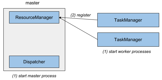
The master process runs a Dispatcher and a ResourceManager in separate threads. Upon start, the TaskManagers register themselves at the ResourceManager.
Figure 9-2 shows how a job is submitted to a stand-alone cluster.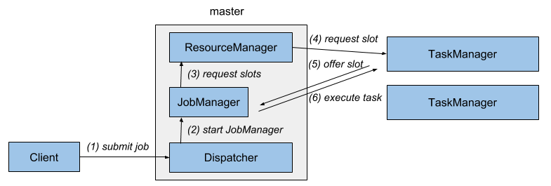
A client submits a job to the dispatcher, which internally starts a JobManager thread and provides the JobGraph for execution. The JobManager requests the necessary processing slots from the ResourceManager and deploys the job for execution once the requested slots have been received.
In a stand-alone deployment, the master and workers are not automatically restarted in case of a failure. A job can recover from a worker failure if a sufficient number of processing slots is available. This can be ensured by running one or more stand-by workers. Job recovery from a master failure requires a highly-available setup as discussed later in this chapter.In order to setup a stand-alone Flink cluster, download a binary distribution from the Apache Flink website and extract the tar archive with the command
tar xfz ./flink-1.5.4-bin-scala_2.11.tgz
The extracted directory includes a ./bin folder with bash scripts1 to start and stop Flink processes. The ./bin/start-cluster.sh script starts a master process on the local machine and one or more TaskManagers on the local or remote machines.
Flink is preconfigured to run a local setup and start a single master and a single TaskManager on the local machine. The start scripts must to be able to start a Java process. If the java binary is not on the PATH, the base folder of a Java installation can be specified by exporting the JAVA_HOME environment variable or setting the env.java.home parameter in ./conf/flink-conf.yaml. A local Flink cluster is started by calling ./bin/start-cluster.sh. You can visit Flink’s WebUI at http://localhost:8081 with your browser and check the number of connected TaskManagers and available slots.
In order to start a distributed Flink cluster that runs on multiple machines, you need to adjust the default configuration and complete a few more setup steps.
The hostnames (or IP addresses) of all machines that should run TaskManagers need to be listed in the ./conf/slaves file.
The start-cluster.sh script requires a passwordless SSH configuration on all machines to be able to start the TaskManager processes.
The Flink distribution folder must be located on all machines at the same path. A common approach is to mount a network-shared directory with the Flink distribution on each machine.
The hostname (or IP address) of the machine that runs the master process needs to be configured in the ./conf/flink-conf.yaml file with the config key jobmanager.rpc.address.
./bin/start-cluster.sh. The script will start a local JobManager and start one TaskManager for each entry in the slaves file. You can check if the master process was started and all TaskManager successfully registered by accessing the WebUI on the machine that runs the master process.
A local or distributed stand-alone cluster is stopped by calling ./bin/stop-cluster.sh.
Docker is a popular platform to package and run applications in containers. Docker containers are run by the operating system kernel of the host system and are therefore more lightweight than virtual machines. Moreover, they are isolated and communicate only through well-defined channels. A container is started from an image which defines the software in the container.
Members of the Flink community configure, build, and upload Docker images for Apache Flink to Docker Hub, a public repository for Docker images2. The repository hosts Docker images for the most recent Flink versions.
Running Flink in Docker is an easy way to setup a Flink cluster on your local machine. For a local Docker setup you have to start two types of containers, a master container which runs the Dispatcher and ResourceManager, and one or more worker containers that run the TaskManagers. The containers work together like a stand-alone deployment (see previous section). Upon start a TaskManager registers itself at the ResourceManager. When a job is submitted to the Dispatcher, it spawns a JobManager thread, which requests processing slots from the ResourceManager. The ResourceManager assigns TaskManagers to the JobManager, which deploys the job once all required resources are available.
Master and worker containers are started from the same Docker image with different parameters as shown in Example 9-1.
// start master process
docker run -d --name flink-jobmanager \
  -e JOB_MANAGER_RPC_ADDRESS=jobmanager \
  -p 8081:8081 flink:1.5 jobmanager

// start worker process (adjust the name to start more than one TM)
docker run -d --name flink-taskmanager-1 \
  --link flink-jobmanager:jobmanager \
  -e JOB_MANAGER_RPC_ADDRESS=jobmanager flink:1.5 taskmanager
Docker will download the requested image and its dependencies from Docker Hub and start the containers running Flink. The Docker internal hostname of the JobManager is passed to the containers via the JOB_MANAGER_RPC_ADDRESS variable, which is used in the entrypoint of the container to adjust Flink’s configuration.
The -p 8081:8081 parameter of the first command maps port 8081 of the master container to port 8081 of the host machine to make the WebUI accessible from the host. You can access the WebUI by opening http://localhost:8081 in your browser. The WebUI can be used to upload application JAR files and run the application. The port also exposes Flink’s REST API. Hence, you can also submit applications using Flink’s CLI client at (./bin/flink), manage running applications, or request information about the cluster or running applications.
Please note that it is currently not possible to pass a custom configuration into the Flink Docker images. You need to build your own Docker image if you want to adjust some parameters. The build scripts of the available Docker Flink images are a good starting point for customized images.
Instead of manually starting two (or more) containers, you can also create a Docker Compose configuration script which automatically starts and configures a Flink custer running in Docker containers and possibly other services such as Zookeeper and Kafka. We will not go into the details of this mode, but among other things, a Docker Compose configuration needs to specify the network configuration such that Flink processes that run in isolated containers can communicate with each other. We refer you to Apache Flink’s documentation for details.
YARN is the resource manager component of Apache Hadoop. It manages compute resources of a cluster environment, i.e., CPU and memory of the cluster’s machines, and provides them to applications that request resources. YARN grants resources as containers3 that are distributed in the cluster and in which applications run their processes. Due to its origin in the Hadoop ecosystem, YARN is typically used by data processing frameworks.
Flink can run on YARN in two modes, the job mode and the session mode. In job mode, a Flink cluster is started to run a single job. Once the job terminates, the Flink cluster is stopped and all resources are returned. Figure 9-3 shows how a Flink job is submitted to a YARN cluster.
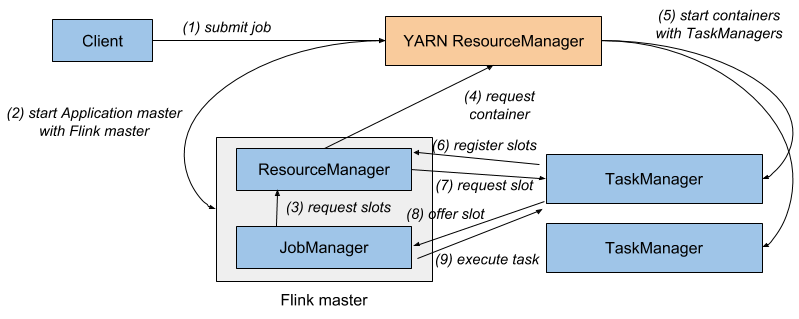
When the client submits a job for execution, it connects to the YARN ResourceManager to start a new YARN application master process that consists of a JobManager thread and a ResourceManager. The JobManager requests the required slots from the ResourceManager to run the Flink job. Subsequently, Flink’s ResourceManager requests containers from YARN’s ResourceManager and starts TaskManager processes. Once started, the TaskManagers register their slots at Flink’s ResourceManager which provides them to the JobManager. Finally, the JobManager submits the job’s tasks to the TaskManagers for execution.
The session mode starts a long-running Flink cluster that can run multiple jobs and needs to be manually stopped. If started in session mode, Flink connects to YARN’s ResourceManager to start an application master that runs of a Dispatcher thread and a Flink ResourceManager thread. Figure 9-4 shows an idle Flink YARN session setup.
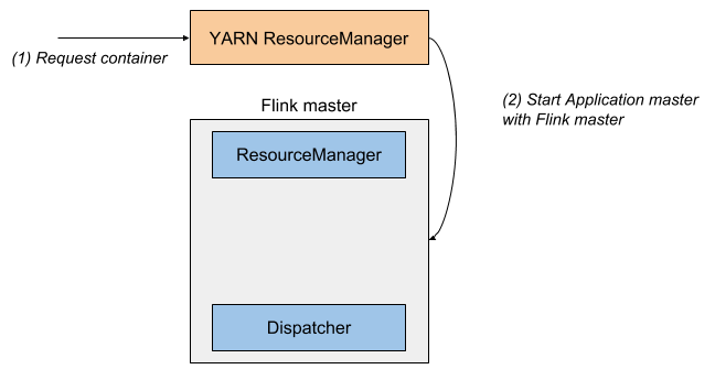
When a job is submitted for execution, the Dispatcher starts a JobManager thread, which requests slots from Flink’s ResourceManager. If not enough slots are available, Flink’s ResourceManager requests additional containers from the YARN ResourceManager to start TaskManager processes which register themselves at the Flink ResourceManager. Once enough slots are available, Flink’s ResourceManager assigns them to the JobManager and the job execution starts. Figure 9-5 shows how a job is executed in Flink’s YARN session mode.
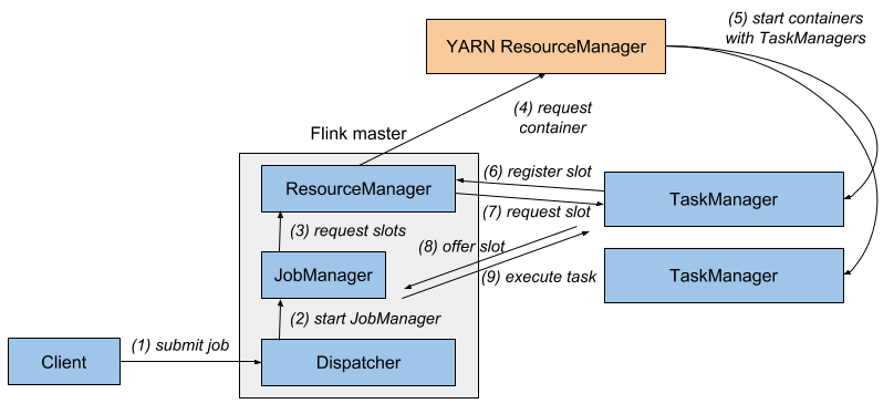
For both setups - job and session mode - failed TaskManagers will be automatically restarted by Flink’s ResourceManager. There are a few parameters in the ./conf/flink-conf.yaml configuration file to control Flink’s recovery behavior on YARN. For example, you can configure the maximum number of failed containers until an application is terminated. In order to recover from master failures, a highly-available setup needs to be configured as described in a later section.
Regardless of whether you run Flink in job or session mode on YARN, it needs to have access to Hadoop dependencies in the correct version and the path to the Hadoop configuration. The later section “Integration with Hadoop Components” describes the required configuration in detail.
Given a working and well configured YARN and HDFS setup, a Flink job can be submitted to be executed on YARN using Flink’s command line client with the following command.
./bin/flink run -m yarn-cluster ./path/to/job.jar
The parameter -m defines the host to which the job is submitted. If set to the keyword yarn-cluster, the client submits the job the the YARN cluster as identified by the Hadoop configuration. Flink’s CLI client supports many more parameters, for example to control the memory of TaskManager containers. Please the check the documentation for a reference. The WebUI of the started Flink cluster is served by the master process runing on some node in the YARN cluster. You can access it via YARN’s WebUI, which provides a link on the Application Overview page under “Tracking URL: ApplicationMaster”.
A Flink YARN session is started with the ./bin/yarn-session.sh script, which also takes various parameters to control the size of containers, the name of the YARN application, or provide dynamic properties. By default, the script prints the connection information of the session cluster and does not return. The session is stopped and all resources are freed when the script is terminated. It is also possible to start a YARN session in detached mode using the -d flag. A detached Flink session can be terminated using YARN’s application utilities.
Once a Flink YARN session is running, you can submit jobs to the session with the following command.
./bin/flink run ./path/to/job.jarNote that you do not need to provide connection information, as Flink memorized the connection details of the Flink session running on YARN. Similar to the job mode, Flink’s WebUI is linked from the Application Overview of YARN’s WebUI.
Kubernetes is an open-source platform to deploy and scale containerized applications in a distributed environment. Given a Kubernetes cluster and an application that is packaged into a container image, you can create a deployment of the application that tells Kubernetes how many instances of the application to start. Kubernetes will run the requested number of containers anywhere on its resources and restart them in case of a failure. Kubernetes can also take care of opening network ports for internal and external communication and can provide services for process discovery and load balancing. Kubernetes runs on on-premise, cloud environment, or hybrid infrastructure.
Deploying data processing frameworks and applications on Kubernetes has become very popular. Apache Flink can be deployed on Kubernetes as well. Before diving into the details of how to setup Flink on Kubernetes, we need to briefly explain a few Kubernetes terms that we will use.A pod is a container [Footnote: Kubernetes also supports pods consisting of multiple tightly-linked containers.] that is started and managed by Kubernetes.
A deployment defines a specific number of pods, i.e., containers to run. Kubernetes ensures that the requested number of pods is continuously running, i.e., automatically restarts failed pods. Deployments can be scaled up or down.
Kubernetes may run a pod anywhere on its cluster. When a pod is restarted after a failure or when deployments are scaled up or down, the IP addresses of pods can change. This is obviously is a problem if pods need to communicate with each other. Kubernetes provides services to overcome the issue of unknown IP addresses. A service defines a policy how a certain group of pods can be accessed. It takes care of updating the routing when a pod is started on a different node in the cluster.
Kubernetes is designed for cluster operations. However, the Kubernetes project provides Minikube, an environment to run a single-node Kubernetes cluster locally on a single machine for testing or daily development. We recommend to setup Minikube if you would like to try to run Flink on Kubernetes and do not have a Kubernetes cluster at hand.
NOTE: In order to successfully run applications on a Flink cluster that is deployed on Minikube, you need to run the following command before deploying Flink.minikube ssh 'sudo ip link set docker0 promisc on'
A Flink setup for Kubernetes is defined with two deployments, one for the pod running the master process and the other for the worker process pods, and a service that exposes the ports of the master pod to the worker pods. The two types of pods, master and worker, behave just like the processes of a stand-alone or Docker deployment that we described before.
The master deployment configuration is shown in Example 9-2.
apiVersion: extensions/v1beta1
kind: Deployment
metadata:
  name: flink-master
spec:
  replicas: 1
  template:
    metadata:
      labels:
        app: flink
        component: master
    spec:
      containers:
      - name: master
        image: flink:1.5
        args:
        - jobmanager
        ports:
        - containerPort: 6123
          name: rpc
        - containerPort: 6124
          name: blob
        - containerPort: 6125
          name: query
        - containerPort: 8081
          name: ui
        env:
        - name: JOB_MANAGER_RPC_ADDRESS
          value: flink-master
The deployment specifies that a single master container should be run (replicas: 1). The master container is started from the Flink 1.5 Docker image (image: flink:1.5) with an argument that starts the master process (args: - jobmanager). Moreover, the deployment configures which ports of the container to open for RPC communication, the blob manager (to exchange large files), the queryable state server, and the Web UI and REST interface.
apiVersion: extensions/v1beta1
kind: Deployment
metadata:
  name: flink-worker
spec:
  replicas: 2
  template:
    metadata:
      labels:
        app: flink
        component: worker
    spec:
      containers:
      - name: worker
        image: flink:1.5
        args:
        - taskmanager
        ports:
        - containerPort: 6121
          name: data
        - containerPort: 6122
          name: rpc
        - containerPort: 6125
          name: query
        env:
        - name: JOB_MANAGER_RPC_ADDRESS
          value: flink-master
The worker deployment looks almost identical to the master deployment with a few differences. First of all, the worker deployment specifies two replicas, which means that two worker containers are started. The worker containers are based on the same Flink Docker image but started with a different argument (args: -taskmanager). Moreover, the deployment also opens a few ports and passes the service name of the Flink master deployment such that the workers can access the master.
The service definition that exposes the master process and makes it accessible to the worker containers is shown in Example 9-4.
apiVersion: v1
kind: Service
metadata:
  name: flink-master
spec:
  ports:
  - name: rpc
    port: 6123
  - name: blob
    port: 6124
  - name: query
    port: 6125
  - name: ui
    port: 8081
  selector:
    app: flink
    component: master
You can create a Flink deployment for Kubernetes by storing each definition in a separate file, such as master-deployment.yaml, worker-deployment.yaml, and master-service.yaml. The files are also provided in our repository. Once you have the definition files, you can register them to Kubernetes using the kubectl command.
kubectl create -f master-deployment.yaml
kubectl create -f worker-deployment.yaml
kubectl create -f master-service.yaml
When running these commands, Kubernetes starts to deploy the requested containers. You can show the status of all deployments by running the following command.
kubectl get deployments
When you create the deployments for the first time, it will take a while until the Flink container image is downloaded. Once all pods are up, you have a Flink cluster running on Kubernetes. However with the given configuration, Kubernetes does not export any port to the outside. Hence, you cannot access the master container to submit an application or access the Web UI. You first need to tell Kubernetes to create a port-forwarding from the master container to your local machine. This is done by running the following command.
kubectl port-forward deployment/flink-master 8081:8081
When the port forwarding is running, you can access the Web UI at the URL http://localhost:8081.
Now you can upload and submit jobs to the Flink cluster running on Kubernetes. Moreover, you can submit applications using the Flink CLI client (./bin/flink) and access the REST interface to request information about the Flink cluster or manage running applications.
When a worker pod fails, Kubernetes will automatically restart the failed pod and the application is recovered (given that checkpointing was activated and properly configured). In order to recover from a master pod failure, you need to configure a highly-available setup.
You can shutdown a Flink cluster running on Kubernetes by running the following commands.
kubectl delete -f master-deployment.yaml
kubectl delete -f worker-deployment.yaml
kubectl delete -f master-service.yaml
Please note that it is not possible to customize the configuration of the Flink deployment with the Flink Docker images that we used in this section. You would need to build custom Docker images with an adjusted configuration. The build script for the provided image ia a good starting point for a custom image.
The support for Kubernetes deployments is still being improved by the Flink community. Flink 1.6 supports an application deployment mode similar to the Yarn job submission mode. In this mode, the Flink application is packaged into a custom container image together with the Flink dependencies. When the application image is deployed to Kubernetes, the Flink processes bootstrap and automatically coordinate themselves.
Most streaming applications are ideally executed continuously with as little downtime as possible. Therefore, many applications must be able to automatically recover from failures of any process that is involved in the execution. While worker failures are handled by the ResourceManager, failures of the JobManager component require the configuration of a highly-available (HA) setup.
Flink’s JobManager holds metadata about an application and its execution, such as the application JAR file, the JobGraph, and pointers to completed checkpoints. This information needs to be recovered in case of a master failure. Flink’s HA mode relies on Apache ZooKeeper, a service for distributed coordination and consistent storage, and a persistent remote storage, such as HDFS, NFS, or S3. The JobManager stores all relevant data in the persistent storage and writes a pointer to the information, i.e., the storage path, to ZooKeeper. In case of a failure, a new JobManager looks up the pointer from ZooKeeper and loads the metadata from the persistent storage. We presented the mode of operation and internals of Flink’s highly-available setup in more detail in Chapter 3. In this section, you will learn how to configure this mode for different deployment options.
A Flink HA setup requires a running Apache ZooKeeper cluster and a persistent remote storage, such as an HDFS, an NFS share, or S3. To help users start a ZooKeeper cluster quickly for testing purposes, Flink provides a helper script for bootstrapping. First, you need to configure the hosts and ports of all ZooKeeper processes involved in the cluster by adjusting the ./conf/zoo.cfg file. Once that is done, you can call ./bin/start-zookeeper-quorum.sh to start a ZooKeeper process on each configured node. Please note that you should not use Flink’s ZooKeeper script for production environments but instead carefully configure and deploy a ZooKeeper cluster yourself.
The Flink HA mode is configured in the ./conf/flink-conf.yaml file by setting the parameters as shown in Example 9-5.
# REQUIRED: enable HA mode via ZooKeeper
high-availability: zookeeper

# REQUIRED: provide a list of all ZooKeeper servers of the quorum
high-availability.zookeeper.quorum: address1:2181[,...],addressX:2181

# REQUIRED: set storage location for job metadata in remote storage
high-availability.zookeeper.storageDir: hdfs:///flink/recovery

# RECOMMENDED: set the base path for all Flink clusters in ZooKeeper.
# Isolates Flink from other frameworks using the ZooKeeper cluster.
high-availability.zookeeper.path.root: /flink
A Flink stand-alone deployment does not rely on a resource provider, such as Yarn or Kubernetes. All processes are manually started and there is no component that monitors these processes and restarts them in case of a failure. Therefore, a stand-alone Flink cluster requires stand-by Dispatcher and TaskManager processes that can take over the work of failed processes.
Besides starting stand-by TaskManagers, a stand-alone deployment does not need additional configuration to be able to recover from TaskManager failures. All started TaskManager processes register themselves at the active ResourceManager. An application can recover from a TaskManager failure as long as enough processing slots are on standby to compensate for the lost TaskManager. The ResourceManager hands out the previously idling processing slots and the application restarts.If configured for high-availability, all Dispatchers of a stand-alone setup register at ZooKeeper. ZooKeeper elects a leader Dispatcher that is responsible for executing applications. When an application is submitted, the responsible Dispatcher starts a JobManager thread which stores its meta data in the configured persistent storage and a pointer in ZooKeeper as discussed before. If the master process that runs the active Dispatcher and JobManager fails, ZooKeeper elects a new Dispatcher as leader. The leading Dispatcher recovers the failed application by starting a new JobManager thread which looks up the metadata pointer in ZooKeeper and loads the metadata from the persistent storage.
In addition to the previously discussed configuration, a highly-available stand-alone deployment requires the following configuration changes. In ./conf/flink-conf.yaml you need to set a cluster identifier for each running cluster. This is required if multiple Flink clusters rely on the same ZooKeeper instance for failure recovery.
# RECOMMENDED: set the path for the Flink cluster in ZooKeeper.
# Isolates multiple Flink clusters from each other.
# The cluster id is required to look up the metadata of a failed cluster.
High-availability.cluster-id: /cluster-1
If you have a ZooKeeper quorum running and Flink properly configured, you can use the regular ./bin/start-cluster.sh script to start a highly-available stand-alone cluster by adding additional hostnames and ports to the ./conf/masters file.
YARN is a cluster resource and container manager. By default, it automatically restarts failed master and TaskManager containers. Hence, you do not need to run standby processes in a YARN setup to achieve high-availability.
Flink’s master process is started as a YARN ApplicationMaster4. YARN automatically restarts a failed ApplicationMaster but tracks and limits the number of restarts to prevent infinite recovery cycles. You need to configure the number of maximum ApplicationManager restarts in the YARN configuration file yarn-site.xml as shown below.
<property>
 <name>yarn.resourcemanager.am.max-attempts</name>
 <value>4</value>
 <description>
   The maximum number of application master execution attempts.
   Default value is 2, i.e., an application is restarted at most once.
 </description>
</property>
Moreover, you need to adjust Flink’s configuration file ./conf/flink-conf.yaml and configure the number of application restart attempts.
# Restart an application at most 3 times (+ the initial start).
# Must be less or equal to the configured maximum number of attempts.
yarn.application-attempts: 4
YARN only counts the number of restarts due to application failures, i.e., restarts due to preemption, hardware failures, or reboots are not taken into account for the number of application attempts. If you run Hadoop YARN version 2.6 or later, Flink automatically configures an attempt failures validity interval. This parameter specifies that an application is only completely canceled if it exceeded its restart attempts within the validity interval, i.e., attempts that predate the interval are not taken into account. Flink configures the interval to the same value as the akka.ask.timeout parameter in ./conf/flink-yaml with a default values of 10 seconds.
./bin/flink run -m yarn-cluster and ./bin/yarn-session.sh. Note that you must configure different cluster-ids for all Flink session clusters that connect to the same ZooKeeper cluster. When starting a Flink cluster in job mode, the cluster-id is automatically set to the id of the started application and is therefore unique.When running Flink on Kubernetes with a master deployment and a worker deployment as described in a previous section, Kubernetes will automatically restart failed containers to ensure that the right number of pods is up and running. This is sufficient to recover from worker failures, which are handed by the ResourceManager. However, recovering from master failures requires additional configuration as discussed before.
In order to enable Flink’s high-availability mode, you need to adjust Flink’s configuration and provide information, such as the hostnames of the ZooKeeper quorum nodes, a path to a persistent storage, and a cluster id for Flink. All of these parameters need to be added to Flink’s configuration file (./conf/flink-conf.yaml). Unfortunately, the Flink Docker image that we used in the Docker and Kubernetes examples before does not support setting custom configuration parameters. Hence, the image cannot be used to setup a highly-available Flink cluster on Kubernetes. Instead you need to build a custom image that either “hardcodes” the required parameters or is flexible enough to adjust the configuration dynamically through parameters or environment variables. The standard Flink Docker images are a good starting point to customize your own Flink images.
Apache Flink can be easily integrated with Hadoop YARN and HDFS, Hadoop’s file system connectors, and other components of the Hadoop ecosystem, such as HBase. In all of these cases, Flink requires Hadoop dependencies on its classpath.
There are three ways to provide Flink with Hadoop dependencies.Use a binary distribution of Flink that was built for a particular Hadoop version. Flink provides builds for the most commonly used vanilla Hadoop versions.
Build Flink for a specific Hadoop version. This is useful if none of Flink’s binary distributions works with the Hadoop version that is deployed in your environment, for example if you run a patched Hadoop version or a Hadoop version of a distributor, such as Cloudera, Hortonworks, or MapR.
In order to build Flink for a specific Hadoop version, you need Flink’s source code, which can be obtained by downloading the source distribution from the website or cloning a stable release branch from the project’s Git repository, a Java JDK of at least version 8, and Apache Maven 3.2. Enter the base folder of Flink’s source code and run one of the commands in the following.
// build Flink for a specific official Hadoop version
mvn clean install -DskipTests -Dhadoop.version=2.6.1

// build Flink for a Hadoop version of a distributor
mvn clean install -DskipTests -Pvendor-repos -Dhadoop.version=2.6.1-cdh5.0.0
The completed build is located in the ./build-target folder.
Use the Hadoop-free distribution of Flink and manually configure the classpath for Hadoop’s dependencies. This approach is useful if none of the provided builds works for your setup. The classpath of the Hadoop dependencies must be declared in the HADOOP_CLASSPATH environment variable. If the variable is not configured, you can automatically set it with the following command if the hadoop command is accessible.
export HADOOP_CLASSPATH=`hadoop classpath`
The classpath option of the hadoop command prints its configured classpath.
HADOOP_CONF_DIR (preferred) or HADOOP_CONF_PATH environment variable. Once Flink knows about Hadoop’s configuration, it is able to connect to YARN’s ResourceManager and HDFS.Apache Flink uses file systems for various tasks. Applications can read their input from and write their results to files (see Chapter 8), application checkpoints and metadata are persisted in remote file systems for recovery (see Chapters 3 and 7), and some internal components leverage file systems to distribute data to tasks, such application JAR files or larger configuration files.
Flink supports a wide variety of file systems. Since Flink is a distributed system and runs processes on cluster or cloud environments, file systems typically need to be globally accessible. Hence, Hadoop HDFS, S3, or NFS and commonly used file systems.Similar to other data processing systems, Flink looks at the URI scheme of a path to identify the file system that the path refers. For example file:///home/user/data.txt points to a file in the local file system and hdfs:///namenode:50010/home/user/data.txt to a file in the specified HDFS cluster.
A file system is represented in Flink by an implementation of the org.apache.flink.core.fs.FileSystem class. The FileSystem class implements file system operations, such as reading from and writing to files, creating directories or files, and listing the content of a directory. A Flink process (JobManager or TaskManager) instantiates one FileSystem object for each configured file system and shares it across all local tasks to guarantee that configured constraints such as limits on the number of open connections are enforced.
Flink provides implementations for the most commonly used file systems.
Local file system, including locally mounted network file systems, such as NFS or SAN. Flink has built-in support for local file systems and does not require additional configuration. Local file systems are referenced by the file:// URI scheme.
Hadoop HDFS. Flink’s connector for HDFS is always in the classpath of Flink. However, it requires Hadoop dependencies on the classpath in order to work. The previous “Integration with Hadoop Components” section explains how to ensure that Hadoop dependencies are loaded. HDFS paths are prefixed with the hdfs:// scheme.
Amazon S3. Flink provides two alternative file system connectors to connect to S3, which are based on Apache Hadoop and Presto. Both connectors are fully self-contained and do not expose any dependencies. To install either of both connectors, move the respective JAR file from the ./opt folder into the ./lib folder. The Flink documentation provides more details on the configuration of S3 file systems. S3 paths are specified with the s3:// scheme.
OpenStack Swift FS. Flink provides a connector to Swift FS which is based on Apache Hadoop. The connector is fully self-contained and does not expose any dependencies. It is installed by moving the respectived JAR file from the ./opt to the ./lib folder. Swift FS paths are identified by the swift:// scheme.
Flink provides a few configuration options in ./conf/flink-conf.yaml to specify a default file system and limit the number of file system connections. You can specify a default file system scheme (fs.default-scheme) that is automatically added as a prefix if a path does not provide a scheme. If you, for example, specify
fs.default-scheme: hdfs://nnode1:9000
the path /result will be extended to hdfs://nnode1:9000/result.
You can limit the number of connections that read from (input) and write to (output) a file system. The configuration can be defined per URI scheme. The relevant configuration keys are listed next.
fs.<scheme>.limit.total: (number, 0/-1 mean no limit)
fs.<scheme>.limit.input: (number, 0/-1 mean no limit)
fs.<scheme>.limit.output: (number, 0/-1 mean no limit)
fs.<scheme>.limit.timeout: (milliseconds, 0 means infinite)
fs.<scheme>.limit.stream-timeout: (milliseconds, 0 means infinite)
The number of connections are tracked per TaskManager process and path authority, i.e.,
hdfs://nnode1:50010 and hdfs://nnode2:50010 are separately tracked. The connection limits can be configured either separately for input and output connections or as total number of connections. When a the file system reached its connection limit and tries to open an new connection, it will block and wait for another connection to close. The timeout parameters define how long to wait until a connection request fails (fs.<scheme>.limit.timeout) and how long to wait until an idle connection is closed (fs.<scheme>.limit.stream-timeout).
You can also provide a custom file system connector. Please have a look at the Flink documentation to learn how to implement and register a custom file system.
Apache Flink offers many parameters to configure behavior and tweak its performance. All parameters can be defined in the ./conf/flink-config.yaml file, which is organized as a flat YAML file of key-value pairs. The configuration file is read by different components, such as the start scripts, the master and worker JVM processes, and the CLI client. For example, the start scripts, like ./bin/start-cluster.sh, parse the configuration file to extract JVM parameters and heap size settings and the CLI client (./bin/flink) extracts the connection information to access the master process. Please note that changes in the configuration file are not effective until Flink is restarted.
To improve the out-of-the-box experience, Flink is pre-configured for a local setup. You need to adjust the configuration to successfully run Flink in distributed environments. In this section, we discuss different aspects that typically need to be configured when setting up a Flink cluster. We refer you to the official documentation for a comprehensive list and detailed description of all parameters.
By default, Flink starts JVM processes using the Java executable that is linked by the PATH environment variable. If Java is not on the PATH or if you want to use a different Java version you can specify the root folder of a Java installation via the JAVA_HOME environment variable or the env.java.home key in the configuration file. Flink’s JVM processes can be started with custom Java options, for example to specify the garbage collector or to enable remote debugging, with the keys env.java.opts, env.java.opts.jobmanager, and env.java.opts.taskmanager.
./lib folder and the user-code classloaders are derived from the system classloader.
By default, Flink looks up user-code classes first in the child (user-code) classloader and then in parent (system) classloader to prevent version clashes in case that a job uses the same dependency as Flink. However, you can also invert the look-up order with the classloader.resolve-order configuration key. Note that some classes are always resolved first in the parent classloader (classloader.parent-first-patterns.default). You can extend the list by providing a whitelist of classname patterns that are first resolved from the parent classloader (classloader.parent-first-patterns.additional).
Flink does not actively limit the amount of CPU resources it consumes. However, it features the concept of processing slots (see Chapter 3 for a detailed discussion) to control the number of tasks that can be assigned to a worker process (TaskManager).
A TaskManager provides a certain number of slots which are registered at and governed by the ResourceManager, A JobManager requests one or more slots to execute an application. Each slot can process one slice of an application, i.e., one parallel task of every operator of the application. Hence, the JobManager needs to acquire at least as many slots as the application’s maximum operator parallelism [footnote: It is possible to assign operators to different slot sharing groups and thereby assign their tasks to distinct slots.]. Tasks are executed as threads within the worker (TaskManager) process and take as much CPU resources as they need.The number of slots that a TaskManager offers is controlled with the taskmanager.numberOfSlots key in the configuration file. The default is 1 slot per TaskManager. The number of slots usually only needs to be configured for stand-alone setups as running Flink on a cluster resource manager (YARN, Kubernetes, Mesos) makes it easy to spin up multiple TaskManagers (each with one slot) per compute node.
Flink’s master and worker processes have different memory requirements. A master process mainly tracks compute resources (ResourceManager) and coordinates the execution of applications (JobManager), while a worker process takes care of the heavy lifting and processes potentially large amounts of data.
Usually, the master process has moderate memory requirements. By default it is started with 1GB JVM heap memory. If a master process needs to execute several applications or an application with many operators, you might need to increase the JVM heap size with thejobmanager.heap.mb configuration key.
Configuring the memory of a worker process is a bit more involved because there are multiple components that need to allocate different types of memory. The most important parameter is the size of the JVM heap memory which is set with the key taskmanager.heap.mb. The heap memory is used for all objects, including the TaskManager runtime, operators and functions of the application, and in-flight data. The state of an application that uses the in-memory of filesystem state backend is also stored on the JVM. You should be aware that a task can consume the whole heap memory of the JVM that it is running on, i.e., Flink does not guarantee or assign heap memory per task or slot. Configurations with a single slot per TaskManager have better resource isolation and can prevent a misbehaving application from interfering with unrelated applications. If you run applications with many dependencies, also the JVM’s non-heap memory can grow to significant size because it stores all TaskManager and user-code classes.
Flink’s default configuration is only suitable for a smaller scale distributed setup and needs to be adjusted for more serious scale. If the number of buffers is not appropriately configured, a job submission will fail with a java.io.IOException: Insufficient number of network buffers. In this case, you should provide more memory to the network stack.
taskmanager.network.memory.fraction key, which determines the fraction of the JVM size that is allocated for network buffers. By default, 10% of the JVM heap size is used. Since the buffers are allocated as off-heap memory, the JVM heap is reduced by that amount. The configuration key taskmanager.memory.segment-size determines the size of a network buffer which is 32KB by default. Reducing the size of a network buffer, increases the number of buffers but can reduce the efficiency of the network stack. You can also specify a minimum and a maximum amount of memory that is used for network buffers (64MB and 1GB by default) to bound the relative configuration value.
RocksDB is another memory consumer that needs to be taken into consideration when configuring the memory of a worker process. Unfortunately, reasoning about the memory consumption of RocksDB is not straightforward because it depends on the number of keyed states in an application. Flink creates a separate (embedded) RocksDB instance for each task of a keyed operator. Within each instance, every distinct state of the operator is stored in a separate column family (or table). With the default configuration, each column family requires about 200MB to 240MB of off-heap memory. You can adjust RocksDB’s configuration and tweak its performance with many parameters.
When configuring the memory setting of a TaskManager, you should size the JVM heap memory such that there is enough memory left for the JVM non-heap memory (classes and meta data) and RocksDB if it is configured as a state backend. Network memory is automatically subtracted from the configured JVM heap size. Keep in mind that some resource managers, such as YARN, will immediately kill a container if it exceeds its memory budget.A Flink worker process stores data on the local file system for multiple reasons, including receiving application JAR files, writing log files, and maintaining application state if the RocksDB state backend is configured. With the io.tmp.dirs configuration key, you can specify one or more directories (separated by colons) that are used to store data in the local file system. By default, data is written to the default temporary directory as determined by the Java system property java.io.tmpdir, i.e., /tmp on Linux and MacOS. The io.tmp.dirs parameter is used as the default value for the local storage path of most components of Flink. However, these paths can also be individually configured.
blob.storage.directory key configures the local storage directory of the blob server, which is used to exchange larger files such as the application JAR files. The env.log.dir key configures the directory into which a TaskManager writes its log files (by default the ./log directory in the Flink setup). Finally, the RocksDB state backend maintains application state in the local file system. The directory is configured using the state.backend.rocksdb.localdir key. If the storage directory is not explicitly configured, RocksDB uses the value of the io.tmp.dirs parameter.Failure recovery is an important aspect of a distributed system. Flink provides several parameters to configure its checkpointing and recovery behavior. Although most options can be explicitly specified within the code of an application, you can also provide default settings through Flink’s configuration file that are applied if job-specific options are not declared.
An important choice that affects the performance of an application is the state backend that is used to maintain the state of the application. You can define the state backend that is used by default with thestate.backend key. Moreover, you can enable asynchronous checkpointing (state.backend.async), incremental checkpointing (state.backend.incremental), and local recovery (state.backend.local-recovery). Note that some options are not supported by all backends. Finally, you can configure the root directories to which checkpoints (state.checkpoints.dir) and savepoints (state.savepoints.dir) are written.
It is also possible to configure the default strategy to restart a failed application (restart-strategy). Possible options are fixed-delay, failure-rate, and none. The strategies can be tuned with additional parameters, such as the number of restart attempts and the delay between restart attempts.
Data processing frameworks are sensitive components of a company’s IT infrastructure and need to be secured against unauthorized access and data retrieval. Apache Flink supports Kerberos authentication and can be configured to encrypt the communication between its processes.
Flink features Kerberos integration with Hadoop and its components (YARN, HDFS, HBase), ZooKeeper, and Kafka. You can enable and configure the Kerberos support for each service separately. Flink supports two authentication modes, keytabs and Hadoop delegation tokens. Keytabs are the preferred approach because tokens expire after some time which can cause problems for long-running stream processing applications. Note that the credentials are tied to a Flink cluster and not to a running job, i.e., all applications that run on the same cluster use the same authentication token. If you need to work with different credentials, you should start a new cluster.While authentication prevents unauthorized access of data or compute resources, encryption ensures that communication partners can trust each other and can share data privately without others being able to listen. Flink supports SSL encryption for the communication between its processes, i.e., the data transfer between TaskManagers, the RPC calls between JobManager and TaskManagers, the blob service transfer, and communication via REST. In order to enable SSL encryption, you need to deploy SSL keystores and truststores on each node that runs a Flink process. Please consult the Flink documentation for detailed instructions to enable and configure Kerberos authentication and SSL encryption.
In this chapter we discussed how Flink is setup in different environments and how to configure highly-available setups. We explained how to enable support for various file systems and how to integrate it with Hadoop and its components. Finally, we discussed the most important configuration options. Note that we did not provide a comprehensive configuration guide. We refer you to the official documentation of Apache Flink for a complete list and detailed descriptions of all configuration options.
1 In order to run Flink on Windows, you can use a provided bat script or you can use the regular bash scripts on the Windows Subsystem for Linux (WSL) or Cygwin. Please note that all scripts only work for local setups.
2 Note that the Flink Docker images are not part of the official Apache Flink release.
3 Note that the concept of a container in YARN is very different from a container in Docker.
4 ApplicationMaster is YARN’s concept for the master process of an application.
Streaming applications are long-running and often their workloads are unpredictable. It is not uncommon for a streaming job to be continuously running for months, so its operational needs are quite different than those of short-lived batch jobs. Consider a scenario where you detect a bug in your deployed application. If your application is a batch job, you can easily fix the bug offline and then re-deploy the new application code once the current job instance finishes. But what if your job is a long-running streaming job? How do you apply a re-configuration with low effort and while guaranteeing correctness?
If you are using Flink, then you have nothing to worry about. Flink will do all the hard work so you can easily monitor, operate, and re-configure your jobs with minimal effort and preserving exactly-once state semantics. In this chapter, we present the tools Flink offers for operating and maintaining continuously running streaming applications. We discuss how you can collect metrics and monitor your applications and how you can preserve result consistency when you want to update application code or adjust the resources of your application.
One would expect that maintaining streaming applications is more challenging than maintaining batch applications. While streaming applications are stateful and continuously running, batch applications are periodically executed. Reconfiguring, scaling, or updating a batch application can be done between executions which seems to be a lot easier than upgrading an application that is continuously ingesting, processing, and emitting data.
However, Apache Flink has many features to significantly ease the maintenance of streaming applications. Most of these features are based on Savepoints. [Footnote: In Chapter 3 we discussed what savepoint are and what you can do with them.]. Flink exposes different interfaces to monitor and control its master and worker processes, and applications.
The command-line client is a tool to submit and control applications.
The REST API is the underlying interface that is used by the command-line client and the WebUI. It can be accessed by users and scripts and provides access to all system and application metrics as well as endpoints to submit and manage applications.
The WebUI is a web interface that provides many details and metrics about a Flink cluster and running applications. It also offers basic functionality to submit and manage applications. The WebUI was described in a later section of this chapter.
In this section, we explain the practical aspects of savepoints and discuss how to start, stop, pause and resume, scale, and upgrade stateful streaming applications using Flink’s command-line client and Flink’s REST API.
A savepoint is basically identical to a checkpoint, i.e., it is a consistent and complete snapshot of an application’s state. However, the life cycles of checkpoints and savepoints differ. Checkpoints are automatically created, loaded in case of a failure, and automatically removed by Flink (depending on the configuration of the application). Moreover, checkpoints are automatically deleted when an application is canceled, unless the application explicitly enabled checkpoint retention. In contrast, savepoints must be manually triggered by a user or an external service and are never automatically removed by Flink.
A savepoint is a directory in a persistent data storage. It consists of a subdirectory that holds the data files containing the state of all tasks and a binary metadata file that includes absolute paths to all data files. Because the paths in the metadata file are absolute, moving a savepoint to a different path will render it unusable. The structure of a savepoint is shown below.
# Savepoint root path
/savepoints/

# Path of a particular savepoint
/savepoints/savepoint-:shortjobid-:savepointid/

# Binary metadata file of a savepoint
/savepoints/savepoint-:shortjobid-:savepointid/_metadata

# Checkpointed operator states
/savepoints/savepoint-:shortjobid-:savepointid/:xxx
Flink’s command-line client provides the functionality to start, stop, and manage Flink applications. It reads its configuration from the ./conf/flink-conf.yaml file (see Chapter 9). You can call it from the root directory of a Flink setup with the command:
./bin/flink
When run without additional parameters, the client prints a help message.
The command-line client is based on a Bash script. Therefore, it does not work with the Windows command-line. The ./bin/flink.bat script for the Windows command-line provides only very limited functionality. If you are a Windows user, we recommend to use the regular command-line client and run it on the Windows Subsystem for Linux (WSL) or Cygwin.
You can start an application with the run command of the command-line client. The command
./bin/flink run ~/myApp.jar
starts the application from the main() method of the class that is referenced in the program-class property of the JAR file’s META-INF/MANIFEST.MF file without passing any arguments to the application. The client submits the JAR file to the master process which distributes it to the worker nodes.
You can pass arguments to the main() method of an application by appending them at the end of the command as shown in the following.
./bin/flink run ~/myApp.jar my-arg1 my-arg2 my-arg3
By default, the client does not return after submitting the application but waits for it to terminate. You can submit an application in detached mode with the -d flag as shown below.
./bin/flink run -d ~/myApp.jar
Instead of waiting for the application to terminate, the client returns and prints the JobID of the submitted job. The JobID is used to specify the job when taking a savepoint, canceling, or rescaling an application.
You can specify the default parallelism of an application with the -p flag.
./bin/flink run -p 16 ~/myApp.jar
The above command sets the default parallelism of the execution environment to 16. The default parallelism of an execution environment is overwritten by all settings that are explicitly specified by the source code of the application, i.e., the parallelism that is defined by calling setParallelism() on the StreamExecutionEnvironment or on an operator has precedence over the default value.
In case the manifest file of your application JAR file does not specify an entry class, you can specify the class using the -c parameter as shown below.
./bin/flink run -c my.app.MainClass ~/myApp.jar
The client will try to start the static main() method of the my.app.MainClass class.
By default, the client submits an application to the Flink master that is specified by the ./conf/flink-conf.yaml file (see the configuration for different setups in Chapter 9). You can submit an application to a specific master process using the -m flag.
./bin/flink run -m myMasterHost:9876 ~/myApp.jar
The above command submits the application to the master that runs on host myMasterHost at port 9876.
Note that the state of an application will be empty if you start it for the first time or do not provide a savepoint or checkpoint to initialize the state. In this case, some stateful operators run special logic to initialize their state. For example, a Kafka source needs to choose the partition offsets from which it consumes a topic if no restored read positions are available.
For all actions that you want to apply to a running job, you need to provide a JobID that identifies the application. The id of a job can be obtained from the WebUI, the REST API, or using the command-line client. The client prints a list of all running jobs, including their JobIDs, when you run the following command.
$ ./bin/flink list -r Waiting for response... ------------------ Running/Restarting Jobs ------------------- 17.10.2018 21:13:14 : bc0b2ad61ecd4a615d92ce25390f61ad : Socket Window WordCount (RUNNING) --------------------------------------------------------------
In the example above the JobID is bc0b2ad61ecd4a615d92ce25390f61ad.
A savepoint can be taken for a running application with the command-line client as follows:
$ ./bin/flink savepoint <jobId> [savepointPath]
The command triggers a savepoint for the job with the provided JobId. If you explicitly specify a savepoint path, the savepoint is stored in the provided directory. Otherwise the default savepoint directory as configured in the flink-conf.yaml file is used.
In order to trigger a savepoint for the job bc0b2ad61ecd4a615d92ce25390f61ad and store it in the directory hdfs:///xxx:50070/savepoints, we call the command-line client as shown below.
$ ./bin/flink savepoint bc0b2ad61ecd4a615d92ce25390f61ad hdfs:///xxx:50070/savepoints
Triggering savepoint for job bc0b2ad61ecd4a615d92ce25390f61ad.
Waiting for response...
Savepoint completed. Path: hdfs:///xxx:50070/savepoints/savepoint-bc0b2a-63cf5d5ccef8
You can resume your program from this savepoint with the run command.
Savepoints can occupy a significant amount of space and are not automatically deleted by Flink. You need to manually remove them to free the consumed storage. A savepoint is removed with the following command.
$ ./bin/flink savepoint -d <savepointPath>
In order to remove the savepoint that we triggered before, call the command as
$ ./bin/flink savepoint -d hdfs:///xxx:50070/savepoints/savepoint-bc0b2a-63cf5d5ccef8 Disposing savepoint 'hdfs:///xxx:50070/savepoints/savepoint-bc0b2a-63cf5d5ccef8'. Waiting for response... Savepoint 'hdfs:///xxx:50070/savepoints/savepoint-bc0b2a-63cf5d5ccef8' disposed.
Note that you must not delete a savepoint before another checkpoint or savepoint completed. Since savepoints are handled by the system very similarly to regular checkpoints, operators also receive checkpoint completion notifications for completed savepoints and act on them. For example, transactional sinks commit changes to external systems when a savepoint completes. In order to guarantee exactly-once output, Flink must recover from the latest completed checkpoint or savepoint. A failure recovery would fail if Flink would attempt to recover from a savepoint that was removed before. Once another checkpoint (or savepoint) completed, you can safely remove a savepoint.
An application can be canceled in two ways, either with or without taking a savepoint. To cancel a running application without taking a savepoint run the following command.
./bin/flink cancel <jobId>
In order to take a savepoint before canceling a running application add the -s flag to the cancel command as shown below.
./bin/flink cancel -s [savepointPath] <jobId>
If you do not specify a savepointPath, the default savepoint directory as configured in ./conf/flink-conf.yaml file is used (see Chapter 9). The command fails if the savepoint folder is neither explicitly specified in the command nor available from the configuration. In order to cancel the application with the JobId bc0b2ad61ecd4a615d92ce25390f61ad and store the savepoint at hdfs:///xxx:50070/savepoints, run the command as shown below.
$ ./bin/flink cancel -s hdfs:///xxx:50070/savepoints d5fdaff43022954f5f02fcd8f25ef855
Cancelling job bc0b2ad61ecd4a615d92ce25390f61ad with savepoint to hdfs:///xxx:50070/savepoints.
Cancelled job bc0b2ad61ecd4a615d92ce25390f61ad. Savepoint stored in hdfs:///xxx:50070/savepoints/savepoint-bc0b2a-d08de07fbb10.</p>
Note that the job will continue to run if taking the savepoint fails. You will need to make another attempt to cancel the job.
Starting an application from a savepoint is fairly simple. All you have to do is to start an application with the run command as discussed before and additionally provide a path to a savepoint with the -s option as show by the command below.
./bin/flink run -s <savepointPath> [options] <jobJar> [arguments]
When the job is started, Flink matches the individual state snapshots of the savepoint to all states of the started application. This matching is done in two steps. First, Flink compares the unique operator identifiers of the savepoint and application’s operators. Second, it matches for each operator the state identifiers (see Chapter 7 for details) of the savepoint and the application.
Note, if you do not assign unique ids to your operators with the uid() method, Flink assigns default identifiers which are hash values that depend on the type of the operator and its predecessors, i.e., all previous operators. Since it is not possible to change the identifiers in a savepoint, you will have much fewer options to update and evolve your application if you do not manually assign operator identifiers using uid().
As mentioned before, an application can only be started from a savepoint if it is compatible with the savepoint. An unmodified application can always be restarted from its savepoint. However if the restarted application is not identical to the application from which the savepoint was taken, there are three cases to consider.
Decreasing or increasing the parallelism of an application is not hard. You need to take a savepoint, cancel the application, and restart it with an adjusted parallelism from the savepoint. The state of the application is automatically redistributed to the larger or smaller number of parallel operator tasks. See the section on “Scaling Stateful Operators” in Chapter 3 for details on how the different types of operator state and keyed state are scaled. However, there are a few things to consider.
If you require exactly-once results, you should take the savepoint and stop the application with the integrated savepoint-and-cancel command. This prevent that another checkpoint completes after the savepoint, which would trigger exactly-once sinks to emit data after the savepoint.
As discussed in the section ”Setting the Parallelism” in Chapter 5, the parallelism of an application and its operators can be specified in different ways. By default, operators run with the default parallelism of their associated StreamExecutionEnvironment. The default parallelism can be specified when starting an application, for example using the -p parameter in the CLI client. If you implement the application such that the parallelism of its operators depends on the default environment parallelism, you can simply scale an application by starting it from the same JAR file and specifying a new parallelism. However, if you hardcoded the parallelism on the StreamExecutionEnvironment or on some of the operators, you might need to adjust the source code, recompile and repackage your application, before submitting it for execution.
If the parallelism of your application depends on the environment’s default parallelism, Flink provides an atomic rescale command which takes a savepoint, cancels the application, and restarts it with a new default parallelism.
./bin/flink modify <jobId> -p <newParallelism>
To rescale the application with the jobId bc0b2ad61ecd4a615d92ce25390f61ad to a parallelism of 16, run the command as shown below.
./bin/flink modify bc0b2ad61ecd4a615d92ce25390f61ad -p 16 Modify job bc0b2ad61ecd4a615d92ce25390f61ad. Rescaled job bc0b2ad61ecd4a615d92ce25390f61ad. Its new parallelism is 16.
As described in Chapter 3, Flink distributes keyed state on the granularity of so-called key groups. Consequently, the number of key groups of a stateful operator determines its maximum parallelism. The number of key groups is configured per operator using the setMaxParallelism() method. Please see Chapter 7 for details.
The REST API can be directly accessed by users or scripts and exposes information about the Flink cluster and its applications, including metrics, as well as endpoints to submit and control applications. Flink serves the REST API and the Web UI from the same web server which runs as part of the Dispatcher process. By default, both are exposed on port 8081. You can configure a different port at the ./conf/flink-conf.yaml file with the configuration key rest.port. A value of -1 disables the REST API and Web UI.
You can access the REST API using the command-line tool curl. curl is commonly used to transfer data from or to a server and supports the HTTP protocol. A typical curl REST command looks as follows.
$ curl -X <HTTP-Method> [-d <parameters>] http://hostname:port/<REST-point>
Assuming that you are running a local Flink setup that exposes its REST API on port 8081, the following curl command submits a GET request to the /overview REST point.
$ curl -X GET http://localhost:8081/overview
The command returns some basic information about the cluster, such as the Flink version, the number of taskmanager, slots, and jobs that are running, finished, cancelled, or failed.
{
 "taskmanagers":2,
 "slots-total":8,
 "slots-available":6,
 "jobs-running":1,
 "jobs-finished":2,
 "jobs-cancelled":1,
 "jobs-failed":0,
 "flink-version":"1.5.3",
 "flink-commit":"614f216"
}
In the following, we list and briefly describe the most important REST calls. Please refer to the official documentation of Apache Flink for a complete list of supported calls. Please note that the previous section about the command-line client provides more details about some of the operations, such as upgrading or scaling an application.
The REST API exposes endpoints to query information about a running cluster and to shut it down.
Get basic information about the cluster
| Request |
GET /overview |
| Response | Basic information about the cluster as shown above. |
Get the configuration of the JobManager
| Request |
GET /jobmanager/config |
| Response | Returns the configuration of the JobManager as defined in the ./conf/flink-conf.yaml. |
Get a list of all connected TaskManagers
| Request |
GET /taskmanagers |
| Response | Returns a list of all TaskManagers including their ids and basic information, such as memory statistics and connection ports. |
Get a list of available JobManager metrics
| Request |
GET /jobmanager/metrics |
| Response | Returns a list of metrics that are available for the JobManager. |
In order to retrieve one or more JobManager metrics, add the get query parameter with all requested metrics to the request as shown below.
curl -X GET http://hostname:port/jobmanager/metrics?get=metric1,metric2,metric3
Get a list of available TaskManager metrics
| Request |
GET /taskmanagers/<tmId>/metrics |
| Parameters | tmId: The ID of a connected TaskManager. |
| Response | Returns a list of metrics that are available for the chosen TaskManager. |
In order to retrieve one or more metrics for a TaskManager, add the get query parameter with all requested metrics to the request as shown below.
curl -X GET http://hostname:port/taskmanagers/<tmId>/metrics?get=metric1,metric2,metric3
Shutdown the cluster
| Request |
DELETE /cluster |
| Action | Shuts down the Flink cluster. Note that in stand-alone mode, only the master process will be terminated and the worker processes will continue to run. |
The REST API can also be used to manage and monitor Flink applications. In order to start an application, you first need to upload the application’s JAR file to the cluster. The REST API provides endpoints to manage these JAR files.
Upload a JAR file
| Request |
POST /jars/upload |
| Parameters | The file must be sent as multi-part data. |
| Action | Uploads a JAR file to the cluster. |
| Response |
The storage location of the uploaded JAR file. |
The curl command to upload a JAR file is shown below.
curl -X POST -H "Expect:" -F "jarfile=@path/to/flink-job.jar" http://hostname:port/jars/upload
List all uploaded JAR files
| Request |
GET /jars |
| Response | A list of all uploaded JAR files. The list includes the internal ID of a JAR file, its original name, and the time when it was uploaded. |
Delete a JAR file
| Request |
DELETE /jars/<jarId> |
| Parameters | jarId: The ID of the JAR file as provided by the list JAR file command. |
| Action |
Deletes the JAR file the is referenced by the provided ID. |
Start an application
| Request |
POST /jars/<jarId>/run |
| Parameters | jarId: The ID of the JAR file from which the application is started.You can pass additional parameters such as the job arguments, the entry-class, the default parallelism, a savepoint path, and the allow-non-restored-state flag as a JSON object. |
| Action | Starts the application defined by the JAR file (and entry-class) with the provided parameters. If a savepoint path is provided, the application state is initialized from the savepoint. |
| Response |
The job ID of the started application. |
The curl command to start an application with a default parallelism of 4 is shown below.
curl -d '{"parallelism":"4"}' -X POST http://localhost:8081/jars/43e844ef-382f-45c3-aa2f-00549acd961e_App.jar/run
List all applications
| Request |
GET /jobs |
| Response | Lists the job IDs of all running applications and the job IDs of the most recently failed, canceled, and finished applications. |
Show details of an application
| Request |
GET /jobs/<jobId> |
| Parameters | jobId: The ID of a job as provided by the list application command. |
| Response | Basic statistics such as the name of the application, the start time (and end time), as well as information about the executed tasks including the number of ingested and emitted records and bytes. |
The REST API also provides more detailed information about the following aspects of an application.
Please have a look at the official documentation for details how to access this information.
Cancel an application
| Request |
PATCH /jobs/<jobId> |
| Parameters | jobId: The ID of a job as provided by the list application command. |
| Action | Cancels the application. |
Take a savepoint of an application
| Request |
POST /jobs/<jobId>/savepoints |
| Parameters | jobId: The ID of a job as provided by the list application command.In addition, you need to provide a JSON object with the path to the savepoint folder and a flag whether or not to terminate the application with the savepoint. |
| Action | Takes a savepoint of the application. |
| Response |
A request ID to check whether the savepoint trigger action completed successfully. |
The curl command to trigger a savepoint without canceling the job looks as follows.
$ curl -d '{"target-directory":"file:///savepoints", "cancel-job":"false"}' -X POST http://localhost:8081/jobs/e99cdb41b422631c8ee2218caa6af1cc/savepoints
{"request-id":"ebde90836b8b9dc2da90e9e7655f4179"}
A request to cancel the application will only succeed if the savepoint was successfully taken, i.e., the application will continue running if the savepoint command failed.
To check if the request with the ID ebde90836b8b9dc2da90e9e7655f4179 was successful and to retrieve the path of the savepoint run the following command.
$ curl -X GET http://localhost:8081/jobs/e99cdb41b422631c8ee2218caa6af1cc/savepoints/ebde90836b8b9dc2da90e9e7655f4179
{"status":{"id":"COMPLETED"}, "operation":{"location":"file:///savepoints/savepoint-e99cdb-34410597dec0"}}
Dispose a savepoint
| Request |
POST /savepoint-disposal |
| Parameters | The path of the savepoint to dispose needs to be provided as a parameter in a JSON object. |
| Action | Disposes a savepoint. |
| Response |
A request ID to check whether the savepoint was successfully disposed or not. |
To dispose a savepoint with curl, run the following command.
$ curl -d '{"savepoint-path":"file:///savepoints/savepoint-e99cdb-34410597dec0"}' -X POST http://localhost:8081/savepoint-disposal
{"request-id":"217a4ffe935ceac2c281bdded76729d6"}
Rescale an application
| Request |
PATCH /jobs/<jobID>/rescaling |
| Parameters |
|
| Action | Takes a savepoint, cancels the application, and restarts it with the new default parallelism from the savepoint. |
| Response | A request ID to check whether the rescaling request was successful or not. |
To rescale an application with curl to a new default parallelism of 16 run the following command.
$ curl -X PATCH http://localhost:8081/jobs/129ced9aacf1618ebca0ba81a4b222c6/rescaling?parallelism=16
{"request-id":"39584c2f742c3594776653f27833e3eb"}
The application will continue to run with the original parallelism if the triggered savepoint failed. You can check the status of the rescale request using
Monitoring your streaming job is essential to ensure its healthy operation and early detect potential symptoms of misconfigurations, under-provisioning, or unexpected behavior. Especially when a streaming job is part of a larger data processing pipeline or event-driven service in a user-facing application, you probably want to monitor its performance as precisely as possible and make sure it meets certain targets for latency, throughput, resource utilization, etc.
Flink gathers a set of pre-defined metrics during runtime and also provides a framework that allows you to define and track your own metrics.
The simplest way to get an overview of your Flink cluster, as well as a glimpse of what your jobs are doing internally is to use Flink’s Web Dashboard. You can access the dashboard by visiting the URL http://<jobmanager-hostname>:8081.
On the home screen, you will see an overview of your cluster configuration including the number of TaskManagers, number of configured, and available task slots, running, and completed jobs. Figure Figure 10-1 shows an instance of the dashboard home screen. The menu on the left links to more detailed information on jobs and configuration parameters and it also allows job submission by uploading a jar.
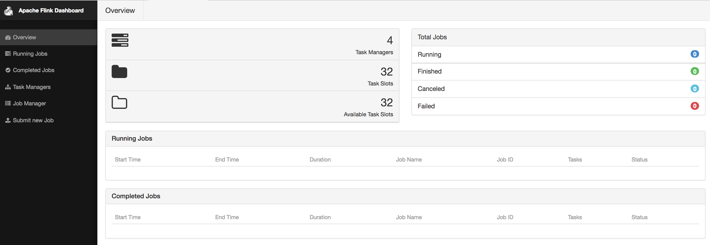
If you click on a running job, you can get a quick glimpse of running statistics per task or subtask as shown in Figure Figure 10-2. You can inspect the duration, bytes and records exchanged, and aggregate those per TaskManager if you prefer.
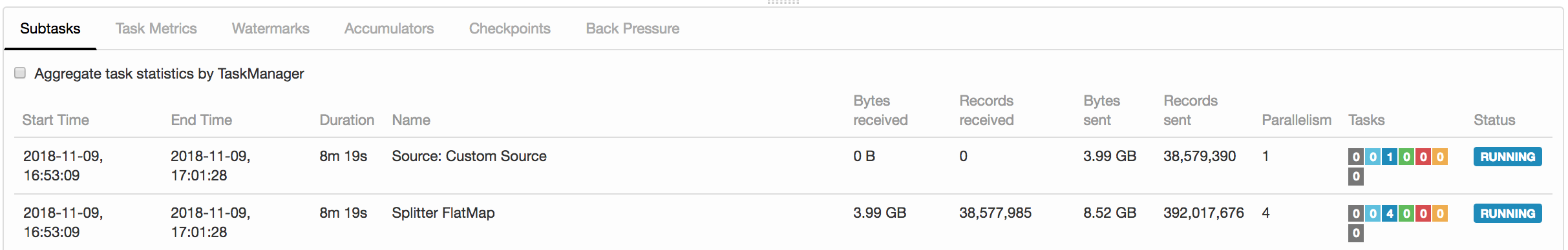
If you click on the Task Metrics tab, you can select more metrics from a drop-down menu, as shown in Figure Figure 10-3. These include more fine-grained statistics about your tasks, such as buffer usage, watermarks, and input/output rates.
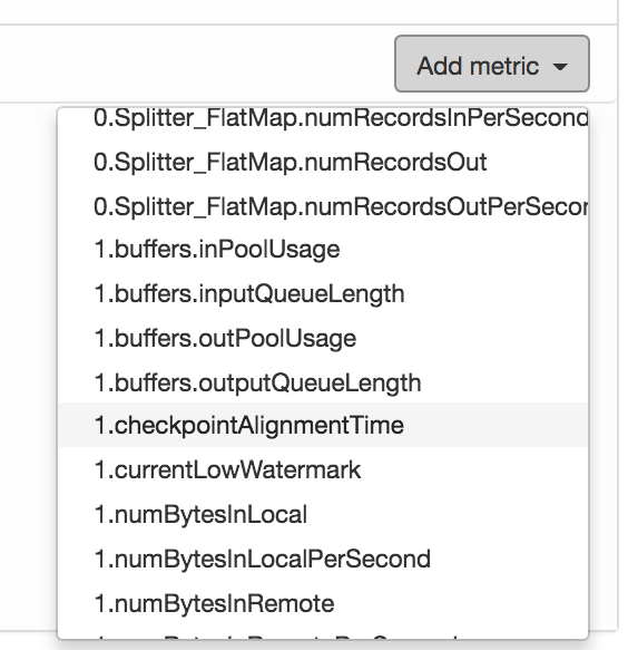
Figure Figure 10-4 shows how selected metrics are visualized as continuously updated charts.
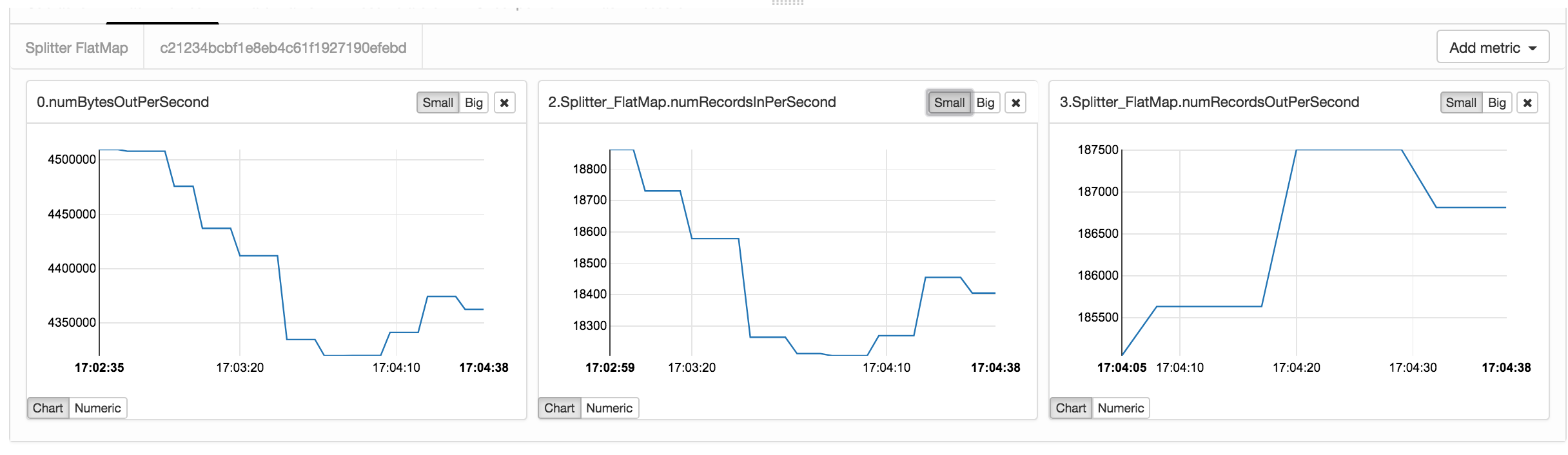
The Checkpoints tab (Figure Figure 10-2) displays statistics about previous and current checkpoints. Under Overview you can see how many checkpoints have been triggered, are in progress, have completed successfully, or have failed. If you click on the History view, you can retrieve more fine-grained information, such as the status, trigger time, state size, and how many bytes where buffered during the checkpoint’s alignment phase. The Summary view aggregates checkpoints statistics and provides minimum, maximum, and average values over all completed checkpoints. Finally, under Configuration, you can inspect the configuration properties of checkpoints, such as the interval and the timeout values set.
Similarly, the Back Pressure tab displays back pressure statistics per operator and subtask. If you click on a row, you trigger back pressure sampling and you will see the message Sampling in progress... for about five seconds. Once sampling is complete, you will see the back pressure status in the second column. Back pressured tasks will display a HIGH sign, otherwise you should see a nice green OK message displayed.
When running a data processing system such as Flink in production, it is essential to monitor its behavior to be able to discover and diagnose the cause for performance degradations. Flink collects several system and application metrics by default. Metrics are gathered per operator, TaskManager, or JobManager. Here we describe some of the most commonly used metrics and refer you to Flink’s documentation for a full list of available metrics.
Categories include CPU utilization, memory used, number of active threads, garbage collection statistics, network metrics such as number of queued input/output buffers, cluster-wide metrics such as number or running jobs and available resources, job metrics including runtime, number of retries and checkpointing information, I/O statistics including number of records exchanges locally and remotely, watermark information, connector-specific metrics, e.g. for Kafka.
Flink metrics are registered and accessed through the MetricGroup interface. The MetricGroup provides ways to create nested, named metrics hierarchies and provides methods to register the following metric types:
Counter
A org.apache.flink.metrics.Counter metric measures a count and provides methods for increment and decrement. You can register a counter metrics using the counter(String name, Counter counter) method on a MetricGroup.
Gauge
A Gauge metric calculates a value of any type at a point in time. To use a Gauge you implement the org.apache.flink.metrics.Gauge interface and register it using the gauge(String name, Gauge gauge) method on a MetricGroup.
The code in Example Example 10-1 shows the implementation of the WatermarkGauge metric which exposes the current watermark:
publicclassWatermarkGaugeimplementsGauge<Long>{privatelongcurrentWatermark=Long.MIN_VALUE;publicvoidsetCurrentWatermark(longwatermark){this.currentWatermark=watermark;}@OverridepublicLonggetValue(){returncurrentWatermark;}}
Metrics reporters will turn the Gauge value into a String, so make sure you provide a meaningful toString() implementation if not provided by the type you use.
Histogram
You can use a histogram to represent the distribution of numerical data. Flink’s histogram is especially implemented for reporting metrics on long values. The org.apache.flink.metrics.Histogram interface allows to collect values, get the current count of collected values, and create statistics, such as min, max, standard deviation, and mean, for the values seen so far.
Apart from creating your own histogram implementation, Flink also allows you to use a DropWizard histogram, by adding the following dependency in pom.xml:
<dependency>
     <groupId>org.apache.flink</groupId>
     <artifactId>flink-metrics-dropwizard</artifactId>
     <version>flink-version</version>
</dependency>
You can then register a DropWizard histogram in your Flink program using the DropwizardHistogramWrapper class as shown in the following example:
DropwizardHistogramWrapperhistogramWrapper=newDropwizardHistogramWrapper(newcom.codahale.metrics.Histogram(newSlidingWindowReservoir(500)))metricGroup.histogram(“myHistogram”,histogramWrapper)…histogramWrapper.update(i)…valminValue=histogramWrapper.getStatistics().getMin()
Meter
You can use a Meter metric to measure the rate (in events per second) at which certain events happen. The org.apache.flink.metrics.Meter interface provides methods to mark the occurrence of one or more events, get the current rate of events per second, and the current number of events marked on the meter.
As with histograms, you can use DropWizard meters by adding the flink-metrics-dropwizard dependency in your pom and wrapping the meter in a DropwizardMeterWrapper class.
In order to register any of the above metrics, you have to retrieve a MetricGroup by calling the getMetrcisGroup() method on the RuntimeContext, as shown in the Example Example 10-4:
classPositiveFilterextendsRichFilterFunction[Int]{@transientprivatevarcounter:Counter=_overridedefopen(parameters:Configuration):Unit={counter=getRuntimeContext.getMetricGroup.counter("droppedElements")}overridedeffilter(value:Int):Boolean={if(value>0){true}else{counter.inc()false}}}
Flink metrics belong to a scope, which can be either the system scope, for system-provided metrics, or the user scope for custom, user-defined metrics.
Metrics are referenced by a unique identifier which contains up to three parts:
For instance, the name “myCounter”, the user scope “MyMetrics”, and the system scope “localhost.taskmanager.512”, would result into the identifier “localhost.taskmanager.512.MyMetrics.myCounter”. You can change the default “." delimiter by setting the metrics.scope.delimiter configuration option.
The system scope declares what component of the system the metric refers to and what context information it should include. Metrics can be scoped to the JobManager, a TaskManager, a job, an operator, or a task. You can configure which context information the metric should contain by setting the corresponding metric options in the flink-conf.yaml file. We list some of these configuration options and their default values in Table Table 10-1:
| Scope | Configuration Key | Default value |
| JobManager | metrics.scope.jm | <host>.jobmanager |
| JobManager and job | metrics.scope.jm.job | <host>.jobmanager.<job_name> |
| TaskManager | metrics.scope.tm | <host>.taskmanager.<tm_id> |
| TaskManager and job | metrics.scope.tm.job |
<host>.taskmanager.<tm_id>.<job_name> |
| Task | metrics.scope.task | <host>.taskmanager.<tm_id>.<job_name>.<task_name>.<subtask_index> |
| Operator | metrics.scope.operator | <host>.taskmanager.<tm_id>.<job_name>.<operator_name>.<subtask_index> |
The configuration keys contain constant strings, such as “taskmanager”, and variables shown in angle brackets. The latter will be replaced at runtime with actual values. For instance, the default scope for TaskManager metrics might create the scope “localhost.taskmanager.512”, where “localhost” and “512" are parameter values. Apart from the ones in the table, the following parameters can also be used:
If multiple copies of the same job are run concurrently, metrics might become inaccurate, due to string conflicts. To avoid such risk, you should make sure that scope identifiers per job are unique. For instance, this can be easily handled by including the job ID.
You can also define a user scope for metrics by calling the addGroup() method of the MetricGroup, as shown in Example Example 10-5:
counter = getRuntimeContext
 .getMetricGroup
 .addGroup("MyMetrics")
 .counter("myCounter")
Now that you have learnt how to register, define, and group metrics, you might be wondering how to access them from external systems. After all, you most probably gather metrics because you want to create a real-time dashboard or feed the measurements to another application. You can expose metrics to external backends through reporters and Flink provides implementation for several of them:
If you want to use a metrics backend that is not included in the above list, you can also define your own reporter by implementing the org.apache.flink.metrics.reporter.MetricReporter interface.
Reporters need to be configured in flink-conf.yaml. Adding the following lines to your configuration will define a JMX reporter “my_reporter" which listens to ports 9020-9040:
metrics.reporters: my_reporter

Metrics.reporter.my_jmx_reporter.class: org.apache.flink.metrics.jmx.JMXReporter

metrics.reporter.my_jmx_reporter.port: 9020-9040
Please consult the Flink documentation for a full list of configuration options per supported reporter.
Latency is probably one of the first metrics you want to monitor to assess the performance characteristics of your streaming job. At the same time, it is also one of the trickiest metrics to even define in a distributed streaming engine with rich semantics such as Flink. In Chapter 2, we defined latency broadly, as the time it takes to process an event. You can imagine how a precise implementation of this definition can get problematic in practice if we try to track the latency per event in a high-rate streaming job with a complex dataflow. Considering window operators complicates latency tracking even further. If an event contributes to several windows, do we need to report the latency of the first invocation or do we need to wait until we evaluate all windows an event might belong to? And what if a window triggers multiple times?
Flink follows a simple and low-overhead approach to provide useful latency metric measurements. Instead of trying to strictly measure latency for each and every event, it approximates latency by periodically emitting a special record at the sources and allowing users to track how long it takes for this record to arrive at the sinks. This special record is called a latency marker and it bears a timestamp indicating when it was emitted.
To enable latency tracking, you need to configure how often latency markers are emitted from the sources. You can do this by setting the latencyTrackingInterval in the ExecutionConfig as shown below:
env.getConfig.setLatencyTrackingInterval(500L
Note that the interval is in specified in milliseconds. Upon receiving a latency marker, all operators except sinks forward it downstream. Latency markers use the same dataflow channels and queues as normal stream records, thus their tracked latency reflects the time records wait to be processed. However, they do not measure the time it takes for records to be processed or the time that records wait in window buffers until they are processed.
Operators keep latency statistics in a latency gauge which contains min, max, and mean values, as well as 50, 95, and 99-percentile values. Sink operators keep statistics on latency markers received per parallel source instance, thus checking the latency marker at sinks can be used to approximate how long it takes for records to traverse the dataflow. If you would like to customly handle the latency marker at operators, you can override the processLatencyMarker() method and retrieve the relevant information using the LatencyMarker’s methods getMarkedTime(), getVertexId(), and getSubTaskIndex().
Note that if you are not using any automatic clock synchronization services such as NTP, your machines' clocks might suffer from clock skew. In this case, latency tracking estimation will not be reliable, as its current implementation assumes synchronized clocks.
Logging is another essential tool for debugging and understanding the behavior of your applications. By default, Flink uses the SLF4J logging abstraction together with the log4j logging framework.
The following example shows a MapFunction that logs every input record conversion:
importorg.apache.flink.api.common.functions.MapFunctionimportorg.slf4j.LoggerFactoryimportorg.slf4j.LoggerclassMyMapFunctionextendsMapFunction[Int,String]{LoggerLOG=LoggerFactory.getLogger(MyMapFunction.class)overridedefmap(value:Int):String={LOG.info("Converting value {} to string.",value)value.toString}}
To change the properties of log4j loggers, you can modify the log4j.properties file in the conf/ folder. For instance, the following line sets the root logging level to “warning”:
log4j.rootLogger=WARN
You can set a custom filename and location of this file passing the -Dlog4j.configuration= parameter to the JVM. Flink also provides the log4j-cli.properties file used by the command-line client and log4j-yarn-session.properties used by the command-line client when starting a YARN session.
An alternative to log4j is logback and Flink provides default configuration files for this backend as well. To use logback instead of log4j, you will need to remove log4j from the lib/ folder. We refer you to Flink’s documentation and the logback manual for details on how to setup and configure the backend.
In this chapter we discussed how to run, manage, and monitor Flink applications in production. We explained the Flink component that collects and exposes system and application metrics, how to configure an logging system, and how to start, stop, resume, and rescale applications with the command line client the the REST API.
First Edition
Fundamentals, Implementation, and Operation of Streaming Applications
Copyright © 2019 Fabian Hueske, Vasiliki Kalavri. All rights reserved.
Printed in the United States of America.
Published by O’Reilly Media, Inc., 1005 Gravenstein Highway North, Sebastopol, CA 95472.
O’Reilly books may be purchased for educational, business, or sales promotional use. Online editions are also available for most titles (http://oreilly.com/safari). For more information, contact our corporate/institutional sales department: 800-998-9938 or corporate@oreilly.com.
See http://oreilly.com/catalog/errata.csp?isbn=XXXXXXXXXXXXX for release details.
The O’Reilly logo is a registered trademark of O’Reilly Media, Inc. Stream Processing with Apache Flink, the cover image, and related trade dress are trademarks of O’Reilly Media, Inc.
While the publisher and the authors have used good faith efforts to ensure that the information and instructions contained in this work are accurate, the publisher and the authors disclaim all responsibility for errors or omissions, including without limitation responsibility for damages resulting from the use of or reliance on this work. Use of the information and instructions contained in this work is at your own risk. If any code samples or other technology this work contains or describes is subject to open source licenses or the intellectual property rights of others, it is your responsibility to ensure that your use thereof complies with such licenses and/or rights.
9781491974223
[???]
Apache Flink is a distributed stream processor with intuitive and expressive APIs to implement stateful stream processing applications. It efficiently runs such applications at large scale in a fault-tolerant manner. Flink joined the Apache Software Foundation as an incubating project in April 2014 and became a top-level project in January 2015. Since its beginning, Flink has a very active and continuously growing community of users and contributors. Until today, more than 350 individuals have contributed to Flink and it has evolved into one of the most sophisticated open source stream processing engines as proven by its widespread adoption. Flink powers large-scale business-critical applications in many companies and enterprises across different industries and around the globe.
Stream processing technology is being rapidly adopted by companies and enterprises of any size because it provides superior solutions for many established use cases but also facilitates novel applications, software architectures, and business opportunities. In this chapter we discuss why stateful stream processing is becoming so popular and assess its potential. We start reviewing conventional data processing application architectures and point out their limitations. Next, we introduce application designs based on stateful stream processing that exhibit many interesting characteristics and benefits over traditional approaches. We briefly discuss the evolution of open source stream processors and help you to run a first streaming application on a local Flink instance. Finally, we tell you what you will learn when reading this book.
Companies employ many different applications to run their business, such as enterprise resource planning (ERP) systems, customer relationship management (CRM) software, or web-based applications. All of these systems are typically designed with separate tiers for data processing (the application itself) and data storage (a transactional database system) as shown in Figure 1-1.
The applications are usually connected to external services or face human users and continuously process incoming events such as orders, or mails, or clicks on a website. When an event is processed, an application reads its state or updates its state by running transactions against the remote database system. Typically, a database system serves multiple applications which often even access the same databases or tables.
This design can cause problems when applications need to evolve or scale. Since, multiple applications might work on the same data representation or share the same infrastructure, changing the schema of a table or scaling a database system requires careful planning and a lot of effort. A recent approach to overcome the tight bundling of applications is the microservice design pattern. Microservices are designed as small, self-contained, and independent applications. They follow the UNIX philosophy of doing a single thing and doing it well. More complex applications are built by connecting several microservices with each other that only communicate over standardized interfaces such as RESTful HTTP connections. Because microservices are strictly decoupled from each other and only communicate over well defined interfaces, each microservice can be implemented with a custom technology stack including programming language, libraries, and data stores. Microservices and all required software and services are typically bundled and deployed in independent containers. Figure 1-2 depicts a microservice architecture.
The data that is stored in the various transactional database systems of a company can provide valuable insights about various aspects of the company’s business. For example, the data of an order processing system can be analyzed to obtain sales growth over time, to identify reasons for delayed shipments, or to predict future sales in order to adjust the inventory. However, transactional data is often distributed across several disconnected database systems and becomes more valuable when it can be jointly analyzed. Moreover, it is often required to transform the data into a common format.
Instead of running analytical queries directly on the transactional databases, a common component in IT systems is a data warehouse. A data warehouse is a specialized database system for analytical query workloads. In order to populate a data warehouse, the data managed by the transactional database systems needs to be copied to it. The process of copying data to the data warehouse is called extract-transform-load (ETL). An ETL process extracts data from a transactional database, transforms it into a common representation which might include validation, value normalization, encoding, de-duplication, and schema transformation, and finally loads it into the analytical database. ETL processes can be quite complex and often require technically sophisticated solutions to meet performance requirements. In order to keep the data of the data warehouse up-to-date, ETL processes need to run periodically.
Once the data has been imported into the data warehouse it can be queried and analyzed. Typically, there are two classes of queries executed on a data warehouse. The first type are periodic report queries that compute business relevant statistics such as revenue, user growth, or production output. These metrics are assembled into reports that help to assess the situation of the business. The second type are ad-hoc queries that aim to provide answers to specific questions and support business-critical decisions. Both kinds of queries are executed by a data warehouse in a batch processing fashion, i.e., the data input of a query is fully available and the query terminates after it returned the computed result. The architecture is depicted in Figure 1-3.
Until the rise of Apache Hadoop, specialized analytical database systems and data warehouses were the predominant solutions for data analytics workloads. However, with the growing popularity of Hadoop, companies realized that a lot of valuable data was excluded from their data analytics process. Often, this data was either unstructured, i.e., not strictly following a relational schema, or too voluminous to be cost-effectively stored in a relational database system. Today, components of the Apache Hadoop ecosystem are integral parts in the IT infrastructures of many enterprises and companies. Instead of inserting all data into a relational database system, significant amounts of data, such as, log files, social media, or web click logs, are written into Hadoop’s distributed file system (HDFS) or other bulk data stores, like Apache HBase, which provide massive storage capacity at small cost. Data that resides in such storage systems is accessible to several SQL-on-Hadoop engines, as for example Apache Hive, Apache Drill, or Apache Impala. However, also with storage systems and execution engines of the Hadoop ecosystem the overall mode of operation of the infrastructure remains basically the same as the traditional data warehouse architecture, i.e., data is periodically extracted and loaded into to a data store and processed by periodic or ad-hoc queries in a batch fashion.
An important observation is that virtually all data is created as continuous streams of events. Think of user interactions on websites or in mobile apps, placements of orders, server logs, or sensor measurements; all of these data are streams of events. In fact, it is difficult to find examples of finite, complete data sets that are generated all at once. Stateful stream processing is an application design pattern for processing unbounded streams of events and is applicable to many different use cases in the IT infrastructure of a company. Before we discuss its use cases, we briefly explain what stateful stream processing is and how it works.
Any application that processes a stream of events and does not just perform trivial record-at-a-time transformations needs to be stateful, i.e., have the ability to store and access intermediate data. When an application receives an event, it can perform arbitrary computations that involve reading data from or writing data to the state. In principle, state can be stored and accessed in many different places including program variables, local files, or embedded or external databases.
Apache Flink stores application state locally in memory or in an embedded database and not in a remote database. Since Flink is a distributed system, the local state needs to be protected against failures to avoid data loss in case of application or machine failures. Flink guarantees this by periodically writing a consistent checkpoint of the application state to a remote and durable storage. State, state consistency, and Flink’s checkpointing mechanism will be discussed in more detail in the following chapters. Figure 1-4 shows a stateful Flink application.
Stateful stream processing applications often ingest their incoming events from an event log. An event log stores and distributes event streams. Events are written to a durable, append-only log which means that the order of written events cannot be changed. A stream that is written to an event log can be read many times by the same or different consumers. Due to the append-only property of the log, events are always published to all consumers in exactly the same order. There are several event log systems available as open source software, Apache Kafka being the most popular, or as integrated services offered by cloud computing providers.
Connecting a stateful streaming application running on Flink and an event log is interesting for multiple reasons. In this architecture the event log acts as a source of truth because it persists the input events and can replay them in an deterministic order. In case of a failure, Flink restores a stateful streaming application by recovering its state from a previously taken checkpoint and resets the read position on the event log.The application will replay (and fast forward) the input events from the event log until it reaches the tail of the stream. This technique is used to recover from failures but can also be leveraged to update an application, fix bugs and repair previously emitted results, migrate an application to a different cluster, or perform A/B tests with different application versions.
As previously stated, stateful streaming processing is a versatile and flexible design pattern and can be used to address many different use cases. In the following we present three classes of applications that are commonly implemented using stateful stream processing, 1) event-driven applications, 2) data pipeline applications, and 3) data analytics applications and give examples of real-world applications. We describe these classes as distinct patterns to emphasize the versatility of stateful stream processing. However, most real-world applications combine characteristics of more than one class which again shows the flexibility of this application design pattern.
Event-driven applications are stateful streaming applications that ingest event streams and apply business logic on the received events. Depending on the business logic, an event-driven application can trigger actions such as sending an alert or an email or write events to an outgoing event stream that is possibly consumed by another event-driven application.
Typical use cases for event-driven applications include
Real-time recommendations, e.g., for recommending products while customers browse on a retailer’s website,
Pattern detection or complex event processing (CEP), e.g., for fraud detection in credit card transactions, and
Anomaly detection, e.g., to detect attempts to intrude a computer network.
Event-driven applications are an evolution of the previously discussed microservices. They communicate via event logs instead of REST calls and hold application data as local state instead of writing it to and reading it from an external data store, such as a transactional database or key-value store. Figure 1-5 sketches a service architecture composed of event-driven streaming applications.
Event-driven applications are an interesting design pattern because they offer several benefits compared to the traditional architecture of separate storage and compute tiers or the popular microservice architectures. Local state accesses, i.e., reading from or writing to memory or local disk, provide very good performance compared to read and write queries against remote data stores. Scaling and fault-tolerance do not need special consideration because these aspects are handled by the stream processor. Finally, by leveraging an event log as input source the complete input of an application is reliably stored and can be deterministically replayed. This is very attractive especially in combination with Flink’s savepoint feature which can reset the state of an application to a previous consistent savepoint. By resetting the state of a (possibly modified) application and replaying the input, it is possible to fix a bug of the application and repair its effects, deploy new versions of an application without losing its state, or run what-if or A/B tests. We know of a company that decided to built the backend of a social network based on an event log and event-driven applications because of these features.
Event-driven applications have quite high requirements on the stream processor that runs them. The business logic is constrained by how much it can control state and time. This aspect depends on the APIs of the stream processor, what kinds of state primitives it provides, and on the quality of its support for event-time processing. Moreover, exactly-once state consistency and the ability to scale an application are fundamental requirements. Apache Flink checks all these boxes and is a very good choice to run event-driven applications.
Today’s IT architectures include many different data stores, such as relational and special-purpose database systems, event logs, distributed file systems, in-memory caches, and search indexes. All of these systems store data in different representations and data structures that provide the best performance for their specific purpose. Subsets of an organization’s data are stored in multiple of these systems. For example, information for a product that is offered in a webshop can be stored in a transactional database, a web cache, and a search index. Due to this replication of data, the data stores must be kept in sync.
The traditional approach of a periodic ETL job to move data between storage systems is typically not able to propagate updates fast enough. Instead a common approach is to write all changes into an event log that serves as source of truth. The event log publishes the changes to consumers that incorporate the updates into the affected data stores. Depending on the use case and data store, the updates need to be processed before they can be incorporated. For example they need to be normalized, joined or enriched with additional data, or pre-aggregated, i.e., transformations that are also commonly performed by ETL processes.
Ingesting, transforming, and inserting data with low latency is another common use case for stateful stream processing applications. We call this type of applications data pipelines. Additional requirements for data pipelines are the ability to process large amounts of data in short time, i.e., support for high throughput, and the capability to scale an application. A stream processor that operates data pipelines should also feature many source and sink connectors to read data from and write data to various storage systems and formats. Again, Flink provides all required features to successfully operate data pipelines and includes many connectors.
Previously in this chapter, we described the common architecture for data analytics pipelines. ETL jobs periodically import data into a data store and the data is processed by ad-hoc or scheduled queries. The fundamental mode of operation - batch processing - is the same regardless whether the architecture is based on a data warehouse or components of the Hadoop ecosystem. While the approach of periodically loading data into data analysis systems has been the state-of-the-art for many years, it suffers from a notable drawback.
Obviously, the periodic nature of the ETL jobs and reporting queries induce a considerable latency. Depending on the scheduling intervals it may take hours or days until a data point is included in a report. To some extent, the latency can be reduced by importing data into the data store with data pipeline applications. However, even with continuous ETL there will always be a certain delay until an event is processed by a query. In the past, analyzing data with a few hours or even days delay was often acceptable because a prompt reaction to new results or insights did not yield a significant advantage. However, this has dramatically changed in the last decade. The rapid digitalization and emergence of connected systems made it possible to collect much more data in real-time and immediately act on this data for example by adjusting to changing conditions or by personalizing user experiences. An online retailer is able to recommend products to users while they are browsing on the retailer’s website; mobile games can give virtual gifts to users to keep them in a game or offer in-game purchases at the right moment; manufacturers can monitor the behavior of machines and trigger maintenance actions to reduce production outages. All these use cases require collecting real-time data, analyzing it with low latency, and immediately reacting to the result. Traditional batch oriented architectures are not able to address such use cases.
You are probably not surprised that stateful stream processing is the right technology to build low-latency analytics pipelines. Instead of waiting to be periodically triggered, a streaming analytics application continuously ingests streams of events and maintains an updating result by incorporating the latest events with low latency. This is similar to view maintenance techniques that database systems use to update materialized views. Typically, streaming applications store their result in an external data store that supports efficient updates, such as a database or key-value store. Alternatively, Flink provides a feature called queryable state which allows users to expose the state of an application as a key-lookup table and make it accessible for external applications. The live updated results of a streaming analytics applications can be used to power dashboard applications as shown in Figure 1-6.
Besides the much smaller time for an event to be incorporated into an analytics result, there is another, less obvious, advantage of streaming analytics applications. Traditional analytics pipelines consist of several individual components such as an ETL process, a storage system, and in case of a Hadoop-based environment also a data processor and scheduler to trigger jobs or queries. These components need to be carefully orchestrated and especially error handling and failure recovery can become challenging.
In contrast, a stream processor that runs a stateful streaming application takes care of all processing steps, including event ingestion, continuous computation including state maintenance, and updating the result. Moreover, the stream processor is responsible to recover from failures with exactly-once state consistency guarantees and should be capable of adjusting the parallelism of an application. Additional requirements to successfully support streaming analytics applications are support for event-time processing in order to produce correct and deterministic results and the ability to process large amounts of data in little time, i.e., high throughput. Flink offers good answers to all of these requirements.
Typical use cases for streaming analytics applications are
Monitoring the quality of cellphone networks.
Analyzing user behavior in mobile applications.
Ad-hoc analysis of live data in consumer technology.
Although not being covered in this book but certainly worth mentioning is that Flink also provides support for analytical SQL queries over streams. Multiple companies have built streaming analytics services based on Flink’s SQL support both for internal use or to publicly offer them to paying customers.
Data stream processing is not a novel technology. First research prototypes and commercial products date back to the late 1990s. However, the growing adoption of stream processing technology in the recent past is driven to a large extent by the availability of mature open source stream processors. Today, distributed open source stream processors power business-critical applications in many enterprises across different industries such as (online) retail, social media, telecommunication, gaming, and banking. Open source software is a major driver of this trend, mainly due to two reasons.
The Apache Software Foundation alone is the home of more than a dozen projects that are related to stream processing. New distributed stream processing projects are continuously entering the open source stage and are challenging the state-of-the-art with new features and capabilities. Often are features of these newcomers being adopted by more stream processors of earlier generations. Moreover, users of open source software request or contribute new features that are missing to support their use cases. This way, open source communities are constantly improving the capabilities of their projects and are pushing the technical boundaries of stream processing further. We will take a brief look into the past to see where open source stream processing came from and where it is today.
The first generation of distributed open source stream processors that got substantial adoption focused on event processing with millisecond latencies and provided guarantees that events would never be lost in case of a failure. These systems had rather low-level APIs and did not provide built-in support for accurate and consistent results of streaming applications because the results depended on the timing and order of arriving events. Moreover, even though events would not be lost in case of a failure, they could be processed more than once. In contrast to batch processors that guarantee accurate results, the first open source stream processors traded result accuracy for much better latency. The observation that data processing systems (at this point in time) could either provide fast or accurate results led to the design of the so-called Lambda architecture which is depicted in Figure 1-7.
The Lambda architecture augments the traditional periodic batch processing architecture with a Speed Layer that is powered by a low-latency stream processor. Data arriving to the Lambda architecture is ingested by the stream processor as well as written to a batch storage such as HDFS. The stream processor computes possibly inaccurate results in near real-time and writes the results into a speed table. The data written to the batch storage is periodically processed by a batch processor. The exact results are written into a batch table and the corresponding inaccurate results from the speed table are dropped. Applications consume the results from the Serving Layer by merging the most recent but only approximated results from the speed table and the older but accurate result from the batch table. The Lambda architecture aimed to improve the high result latency of the original batch analytics architecture. However, the approach had a few notable drawbacks. First of all, it requires two semantically equivalent implementations of the application logic for two separate processing systems with different APIs. Second, the latest results computed by the stream processor are not accurate but only approximated. Third, the Lambda architecture is hard to setup and maintain. A textbook setup consists of a stream processor, a batch processor, a speed store, a batch store, and tools to ingest data for the batch processor and scheduling batch jobs.
Improving on the first generation, the next generation of distributed open source stream processors provided better failure guarantees and ensured that in case of a failure each record contributes exactly once to the result. In addition, programming APIs evolved from rather low-level operator interfaces to high-level APIs with more built-in primitives. However, some improvements such as higher throughput and better failure guarantees came at the cost of increasing processing latencies from milliseconds to seconds. Moreover, results were still dependent on timing and order of arriving events, i.e., the results did not depend solely on the data but also on external conditions such as the hardware utilization.
The third generation of distributed open source stream processors fixed the dependency of results on the timing and order of arriving events. In combination with exactly-once failure semantics, systems of this generation are the first open source stream processors that are capable of computing consistent and accurate results. By computing results only based on the actual data, these systems are also able to process historical data in the same way as “live” data, i.e., data which is ingested as soon as it is produced. Another improvement was the dissolution of the latency-throughput trade-off. While previous stream processors only provided either high throughput or low latency, systems of the third generation are able to serve both ends of the spectrum. Stream processors of this generation made the lambda architecture obsolete.
In addition to the system properties discussed so far, such as failure tolerance, performance, and result accuracy, stream processors also continuously added new operational features. Since streaming applications are often required to run 24/7 with minimum downtime, many stream processors added features such as highly-available setups, tight integration with resource managers, such as YARN or Mesos, and the ability to dynamically scale streaming applications. Other features include support to upgrade application code or migrating a job to a different cluster or a new version of the stream processor without losing the current state of an application.
Apache Flink is a distributed stream processor of the third generation with a competitive feature set. It provides accurate stream processing with high throughput and low latency at scale. In particular the following features let it stand out:
Flink supports event-time and processing-time semantics. Event-time provides consistent and accurate results despite out-of-order events. Processing-time can be applicable for applications with very low latency requirements.
Flink supports exactly-once state consistency guarantees.
Flink achieves millisecond latencies and is able to process millions of events per second. Flink applications can be scaled to run on thousands of cores.
Flink features layered APIs with varying tradeoffs for expressiveness and ease-of-use. This book covers the DataStream API and the ProcessFunction which provide primitives for common stream processing operations, such as windowing and asynchronous operations, and interfaces to precisely control state and time. Flink’s relational APIs, SQL and the LINQ-style Table API, are not discussed in this book.
Flink provides connectors to the most commonly used storage systems such as Apache Kafka, Apache Cassandra, Elasticsearch, JDBC, Kinesis, and (distributed) file systems such as HDFS and S3.
Flink is able to run streaming applications 24/7 with very little downtime due to its highly-available setup (no single point of failure), a tight integration with YARN and Apache Mesos, fast recovery from failures, and the ability to dynamically scale jobs.
Flink allows for updating the application code of jobs and migrating jobs to different Flink clusters without losing the state of the application.
Detailed and customizable collection of system and application metrics help to identify and react to problems ahead of time.
Last but not least, Flink is also a full-fledged batch processor.
In addition to these features, Flink is a very developer-friendly framework due to its easy-to-use APIs. An embedded execution mode starts Flink applications as a single JVM process which can be used to run and debug Flink jobs within an IDE. This feature comes in handy when developing and testing Flink applications.
Next, we will guide you through the process of starting a local cluster and executing a first streaming application in order to give you a first impression of Flink. The application we are going to run converts and aggregates randomly generated temperature sensor readings by time. For this your system needs to have Java 8 (or a later version) installed. We describe the steps for a UNIX environment. If you are running Windows, we recommend to set up a virtual machine with Linux, Cygwin (a Linux environment for Windows), or the Windows Subsystem for Linux, which was introduced with Windows 10.
Go to the Apache Flink webpage flink.apache.org and download the Hadoop-free binary distribution of Apache Flink 1.4.0.
Extract the archive file
tar xvfz flink-1.4.0-bin-scala_2.11.tgz
Start a local Flink cluster
cd flink-1.4.0

	./bin/start-cluster.sh
Open the web dashboard on by entering the URL http://localhost:8081 in your browser. As shown in Figure 1-8, you will see some statistics about the local Flink cluster you just started. It will show that a single Task Manager (Flink’s worker processes) is connected and that a single Task Slot (resource units provided by a Task Manager) is available.
Download the JAR file that includes all example programs of this book.
wget https://streaming-with-flink.github.io/examples/download/examples-scala.jar
Note: you can also build the JAR file yourself by following the steps on the repository’s README file.
Run the example on your local cluster by specifying the applications entry class and the JAR file
./bin/flink run -c io.github.streamingwithflink.AverageSensorReadings examples-scala.jar
Inspect the web dashboard. You should see a job listed under “Running Jobs”. If you click on that job you will see the data flow and live metrics about the operators of the running job similar to the screenshot in Figure 1-9.
The output of the job is written to the standard out of Flink’s worker process which is by default redirected into a file in the ./log folder. You can monitor the constantly produced output using the tail command for example as follows
tail -f ./log/flink-<user>-jobmanager-<hostname>.out
You should see lines as the following ones being written to the file
SensorReading(sensor_2,1480005737000,18.832819812267438)

	SensorReading(sensor_5,1480005737000,52.416477673987856)

	SensorReading(sensor_3,1480005737000,50.83979980099426)

	SensorReading(sensor_4,1480005737000,-17.783076985394775)
The output can be read as follows: the first field of the SensorReading is a sensorId, the second field is the timestamp as milliseconds since 1970-01-01-00:00, and the third field is an average temperature computed over five seconds.
Since you are running a streaming application, it will continue to run until you cancel it. You can do this by selecting the job in the web dashboard and clicking on the CANCEL button on the top of the page.
Finally, you should stop the local Flink cluster
./bin/stop-cluster.sh
That’s it. You just installed and started your first local Flink cluster and ran your first Flink DataStream program! Of course there is much more to learn about stream processing with Apache Flink and that’s what this book is about.
This book will teach you everything to know about stream processing with Apache Flink. Chapter 2 discusses fundamental concepts and challenges of stream processing and Chapter 3 the system architecture of Flink to address these requirements. Chapters 4 to 8 guide you through setting up a development environment, cover the basics of the DataStream API, and go into the details of Flink’s time semantics and window operators, its connectors to external systems, and the details of Flink’s fault-tolerant operator state. Chapter 9 discusses how to setup and configure Flink clusters in various environments and finally Chapter 10 how to operate, monitor, and maintain streaming applications that run 24/7.
So far, you have seen how stream processing addresses limitations of traditional batch processing and how it enables new applications and architectures. You have become familiar with the evolution of the open-source stream processing space and you have got a brief taste of what a Flink streaming application looks like. In this chapter, you will enter the streaming world for good and you will get the necessary background for the rest of this book.
This chapter is still rather independent of Flink. Its goal is to introduce the fundamental concepts of stream processing and discuss the requirements of stream processing frameworks. We hope that after reading this chapter, you will have gained a better understanding of stream applications requirements and you will be able to evaluate the features of modern stream processing systems.
Before we delve into the fundamentals of stream processing, we must first introduce the necessary background on dataflow programming and establish the terminology that we will use throughout this book.
As the name suggests, a dataflow program describes how data flows between operations. Dataflow programs are commonly represented as directed graphs, where nodes are called operators and represent computations and edges represent data dependencies. Operators are the basic functional units of a dataflow application. They consume data from inputs, perform a computation on them, and produce data to outputs for further processing. Operators without input ports are called data sources and operators without output ports are called data sinks. A dataflow graph must have at least one data source and one data sink. Figure 2.1 shows a dataflow program that extracts and counts hashtags from an input stream of tweets.
Dataflow graphs like the one of Figure 2.1 are called logical because they convey a high-level view of the computation logic. In order to execute a dataflow program, its logical graph is converted into a physical dataflow graph, which includes details about how the computation is going to be executed. For instance, if we are using a distributed processing engine, each operator might have several parallel tasks running on different physical machines. Figure 2.2 shows a physical dataflow graph for the logical graph of Figure 2.1. While in the logical dataflow graph the nodes represent operators, in the physical dataflow, the nodes are tasks. The “Extract hashtags” and “Count” operators have two parallel operator tasks, each performing a computation on a subset of the input data.
You can exploit parallelism in dataflow graphs in different ways. First, you can partition your input data and have tasks of the same operation execute on the data subsets in parallel. This type of parallelism is called data parallelism. Data parallelism is useful because it allows for processing large volumes of data and spreading the computation load across several computing nodes. Second, you can have tasks from different operators performing computations on the same or different data in parallel. This type of parallelism is called task parallelism. Using task parallelism you can better utilize the computing resources of a cluster.
Data exchange strategies define how data items are assigned to tasks in a physical dataflow graph. Data exchange strategies can be automatically chosen by the execution engine depending on the semantics of the operators or explicitly imposed by the dataflow programmer. Here, we briefly review some common data exchange strategies, as shown in Figure 2.3.
The forward strategy and the random strategy can also be viewed as variations of the key-based strategy, where the first preserves the key of the upstream tuple while the latter performs a random re-assignment of keys.
Now that you have become familiar with the basics of dataflow programming, it’s time to see how these concepts apply to processing data streams in parallel. But first, we define the term data stream:
A data stream is a potentially unbounded sequence of events
Events in a data stream can represent monitoring data, sensor measurements, credit card transactions, weather station observations, online user interactions, web searches, etc. In this section, you are going to learn the concepts of processing infinite streams in parallel, using the dataflow programming paradigm.
In the previous chapter, you saw how streaming applications have different operational requirements from traditional batch programs. Requirements also differ when it comes to evaluating performance. For batch applications, we usually care about the total execution time of a job, or how long it takes for our processing engine to read the input, perform the computation, and write back the result. Since streaming applications run continuously and the input is potentially unbounded, there is no notion of total execution time in data stream processing. Instead, streaming applications must provide results for incoming data as fast as possible while being able to handle high ingest rates of events. We express these performance requirements in terms of latency and throughput.
Latency indicates how long it takes for an event to be processed. Essentially, it is the time interval between receiving an event and seeing the effect of processing this event in the output. To understand latency intuitively, consider your daily visit to your favorite coffee shop. When you enter the coffee shop, there might be other customers inside already. Thus, you wait in line and when it is your turn you make an order. The cashier receives your payment and passes your order to the barista who prepares your beverage. Once your coffee is ready, the barista calls your name and you can pick up your coffee from the bench. Your service latency is the time you spend in the coffee shop, from the moment you enter until you have the first sip of coffee.
In data streaming, latency is measured in units of time, such as milliseconds. Depending on the application, you might care about average latency, maximum latency, or percentile latency. For example, an average latency value of 10ms means that events are processed within 10ms on average. Instead, a 95th-percentile latency value of 10ms means that 95% of events are processed within 10ms. Average values hide the true distribution of processing delays and might make it hard to detect problems. If the barista runs out of milk right before preparing your cappuccino, you will have to wait until they bring some from the supply room. While you might get annoyed by this delay, most other customers will still be happy.
Ensuring low latency is critical for many streaming applications, such as fraud detection, raising alarms, network monitoring, and offering services with strict service level agreements (SLAs). Low latency is a key characteristic of stream processing and it enables what we call real-time applications. Modern stream processors, like Apache Flink, can offer latencies as low as a few milliseconds. In contrast, traditional batch processing latencies typically range from a few minutes to several hours. In batch processing you first need to gather the events in batches and only then you are able to process them. Thus, the latency is bounded by the arrival time of the last event in each batch and naturally depends on the batch size. True stream processing does not introduce such artificial delays and therefore can achieve really low latencies. In a true streaming model, events can be processed as soon as they arrive in the system and latency more closely reflects the actual work that has to performed on each event.
Throughput is a measure of the system’s processing capacity, i.e. its rate of processing. That is, throughput tells us how many events the system can process per time unit. Revisiting the coffee shop example, if the shop is open from 7am to 7pm and it serves 600 customers in one day, then its average throughput would be 50 customers per hour. While you want latency to be as low as possible, you generally want throughput to be as high as possible.
Throughput is measured in events or operations per time unit. It is important to note that the rate of processing depends on the rate of arrival; low throughput does not necessarily indicate bad performance. In streaming systems you usually want to ensure that your system can handle the maximum expected rate of events. That is, you are primarily concerned with determining the peak throughput, i.e. the performance limit when your system is at its maximum load. To better understand the concept of peak throughput, let us consider that system resources are completely unused. As the first event comes in, it will be immediately processed with the minimum latency possible. If you are the first customer showing up at the coffee shop right after it opened its doors in the morning, you will be served immediately. Ideally, you would like this latency to remain constant and independent of the rate of the incoming events. However, once we reach a rate of incoming events such that the system resources are fully used, we will have to start buffering events. In the coffee shop example, you will probably see this happening right after lunch. Many people show up at the same time and you have to wait in line to place your order. At this point the system has reached the peak throughput and further increasing the event rate will only result in worse latency. If the system continues to receive data at a higher rate than it can handle, buffers might become unavailable and data might get lost. This situation is commonly known as backpressure and there exist different strategies to deal with it. In Chapter 3, we look at Flink’s backpressure mechanism in detail.
At this point, it should be quite clear that latency and throughput are not independent metrics. If events take long to travel in the data processing pipeline, we cannot easily ensure high throughput. Similarly, if a system’s capacity is small, events will be buffered and have to wait before they get processed.
Let us revisit the coffee shop example to clarify how latency and throughput affect each other. First, it should be clear that there is an optimal latency in the case of no load. That is, you will get the fastest service if you are the only customer in the coffee shop. However, during busy times, customers will have to wait in line and latency will increase. Another factor that affects latency and consequently throughput is the time it takes to process an event, or the time it takes for each customer to be served in the coffee shop. Imagine that during Christmas holiday season, baristas have to draw a Santa Claus on the cup of each coffee they serve. This way, the time to prepare a single beverage will increase, causing each person to spend more time in the coffee shop, thus lowering the overall throughput.
Then, can you somehow get both low latency and high throughput or is this a hopeless endeavour? One way you can lower latency is by hiring a more skilled barista, i.e. one that prepares coffees faster. At high load, this change will also increase throughput, because more customers will be served in the same amount of time. Another way to achieve the same result is to hire a second barista, that is, to exploit parallelism. The main take-away here is that lowering latency actually increases throughput. Naturally, if a system can perform operations faster, it can perform more operations at the same amount of time. In fact, that is what you achieve by exploiting parallelism in a stream processing pipeline. By processing several streams in parallel, you can lower the latency while processing more events at the same time.
Stream processing engines usually provide a set of built-in operations to ingest, transform, and output streams. These operators can be combined into dataflow processing graphs to implement the logic of streaming applications. In this section, we describe the most common streaming operations.
Operations can be either stateless or stateful. Stateless operations do not maintain any internal state. That is, the processing of an event does not depend on any events seen in the past and no history is kept. Stateless operations are easy to parallelize, since events can be processed independently of each other and of their arriving order. Moreover, in the case of a failure, a stateless operator can be simply restarted and continue processing from where it left off. On the contrary, stateful operators may maintain information about the events they have received before. This state can be updated by incoming events and can be used in the processing logic of future events. Stateful stream processing applications are more challenging to parallelize and operate in a fault tolerant manner because state needs to be efficiently partitioned and reliably recovered in the case of failures. You will learn more about stateful stream processing, failure scenarios, and consistency in the end of this chapter.
Data ingestion and data egress operations allow the stream processor to communicate with external systems. Data ingestion is the operation of fetching raw data from external sources and converting it into a format that is suitable for processing. Operators that implement data ingestion logic are called data sources. A data source can ingest data from a TCP socket, a file, a Kafka topic, or a sensor data interface. Data egress is the operation of producing output in a form that is suitable for consumption by external systems. Operators that perform data egress are called data sinks and examples include files, databases, message queues, and monitoring interfaces.
Transformation operations are single-pass operations that process each event independently. These operations consume one event after the other and apply some transformation to the event data, producing a new output stream. The transformation logic can be either integrated in the operator or provided by a user-defined function (UDF), as shown in Figure 2.4. UDFs are written by the application programmer and implement custom computation logic.
Operators can accept multiple inputs and produce multiple output streams. They can also modify the structure of the dataflow graph by either splitting a stream into multiple streams or merging streams into a single flow. We discuss the semantics of all operators available in Flink in Chapter 5.
A rolling aggregation is an aggregation, such as sum, minimum, and maximum, that is continuously updated for each input event. Aggregation operations are stateful and combine the current state with the incoming event to produce an updated aggregate value. Note that to be able to efficiently combine the current state with an event and produce a single value, the aggregation function must be associative and commutative. Otherwise, the operator would have to store the complete stream history. Figure 2.5 shows a rolling minimum aggregation. The operator keeps the current minimum value and accordingly updates it for each incoming event.
Transformations and rolling aggregations process one event at a time to produce output events and potentially update state. However, some operations must collect and buffer records to compute their result. Consider for example a streaming join operation or a holistic aggregate, such as median. In order to evaluate such operations efficiently on unbounded streams, you need to limit the amount of data these operations maintain. In this section, we discuss window operations, which provide such a mechanism.
Apart from having a practical value, windows also enable semantically interesting queries on streams. You have seen how rolling aggregations encode the history of the whole stream in an aggregate value and provide us with a low-latency result for every event. This is fine for some applications, but what if you are only interested in the most recent data? Consider an application that provides real-time traffic information to drivers so that they can avoid congested routes. In this scenario, you want to know if there has been an accident in a certain location within the last few minutes. On the other hand, knowing about all accidents that have ever happened might not be so interesting in this case. What’s more, by reducing the stream history to a single aggregate, you lose the information about how your data varies over time. For instance, you might want to know how many vehicles cross an intersection every 5 minutes.
Window operations continuously create finite sets of events called buckets from an unbounded event stream and let us perform computations on these finite sets. Events are usually assigned to buckets based on data properties or based on time. To properly define window operator semantics, we need to answer two main questions: “how are events assigned to buckets?” and “how often does the window produce a result?”. The behavior of windows is defined by a set of policies. Window policies decide when new buckets are created, which events are assigned to which buckets, and when the contents of a bucket get evaluated. The latter decision is based on a trigger condition. When the trigger condition is met, the bucket contents are sent to an evaluation function that applies the computation logic on the bucket elements. Evaluation functions can be aggregations like sum or minimum or custom operations applied on the bucket’s collected elements. Policies can be based on time (e.g. events received in the last 5 seconds), on count (e.g. the last 100 events), or on a data property. In this section, we describe the semantics of common window types.
All the window types that you have seen so far are global windows and operate on the full stream. In practice though you might want to partition a stream into multiple logical streams and define parallel windows. For instance, if you are receiving measurements from different sensors, you probably want to group the stream by sensor id before applying a window computation. In parallel windows, each partition applies the window policies independently of other partitions. Figure 2.10 shows a parallel count-based tumbling window of length 2 which is partitioned by event color.
Window operations are closely related to two dominant concepts in stream processing: time semantics and state management. Time is perhaps the most important aspect of stream processing. Even though low latency is an attractive feature of stream processing, its true value is way beyond just offering fast analytics. Real-world systems, networks, and communication channels are far from perfect, thus streaming data can often be delayed or arrive out-of-order. It is crucial to understand how you can deliver accurate and deterministic results under such conditions. What’s more, streaming applications that process events as they are produced should also be able to process historical events in the same way, thus enabling offline analytics or even time travel analyses. Of course, none of this matters if your system cannot guard state against failures. All the window types that you have seen so far need to buffer data before performing an operation. In fact, if you want to compute anything interesting in a streaming application, even a simple count, you need to maintain state. Considering that streaming applications might run for several days, months, or even years, you need to make sure that state can be reliably recovered under failures and that your system can guarantee accurate results even if things break. In the rest of this chapter, we are going to look deeper into the concepts of time and state guarantees under failures in data stream processing.
In this section, we introduce time semantics and describe the different notions of time in streaming. We discuss how a stream processor can provide accurate results with out-of-order events and how you can perform historical event processing and time travel with streaming.
When dealing with a potentially unbounded stream of continuously arriving events, time becomes a central aspect of applications. Let’s assume you want to compute results continuously, for example every one minute. What would one minute really mean in the context of our streaming application?
Consider a program that analyzes events generated by users playing online mobile games. Users are organized in teams and the application collects a team’s activity and provides rewards in the game, such as extra lives and level-ups, based on how fast the team’s members meet the game’s goals. For example, if all users in a team pop 500 bubbles within one minute, they get a level-up. Alice is a devoted player who plays the game every morning during her commute to work. The problem is that Alice lives in Berlin and she takes the subway to work. And everyone knows that the mobile internet connection in the Berlin subway is lousy. Consider the case where Alice starts popping bubbles while her phone is connected to the network and sends events to the analysis application. Then suddenly, the train enters a tunnel and her phone gets disconnected. Alice keeps on playing and the game events are buffered in her phone. When the train exits the tunnel, she comes back online, and pending events are sent to the application. What should the application do? What’s the meaning of one minute in this case? Does it include the time Alice was offline or not?
Online gaming is a simple scenario showing how operator semantics should depend on the time when events actually happen and not the time when the application receives the events. In the case of a mobile game, consequences can be as bad as Alice and her team getting disappointed and never playing again. But there are much more time-critical applications whose semantics we need to guarantee. If we only consider how much data we receive within one minute, our results will vary and depend on the speed of the network connection or the speed of the processing. Instead, what really defines the amount of events in one minute is the time of the data itself.
In Alice’s game example, the streaming application could operate with two different notions of time, Processing time or Event time. We describe both notions in the following sections.
Processing time is the time of the local clock on the machine where the operator processing the stream is being executed. A processing-time window includes all events that happen to have arrived at the window operator within a time period, as measured by the wall-clock of its machine. As shown in Figure 2-12, in Alice’s case, a processing-time window would continue counting time when her phone gets disconnected, thus not accounting for her game activity during that time.
Event-time is the time when an event in the stream actually happened. Event time is based on a timestamp that is attached on the events of the stream. Timestamps usually exist inside the event data before they enter the processing pipeline (e.g. event creation time). Figure 2-13 shows that an event-time window would correctly place events in a window, reflecting the reality of how things happened, even though some events were delayed.
Event-time completely decouples the processing speed from the results. Operations based on event-time are predictable and their results deterministic. An event-time window computation will yield the same result no matter how fast the stream is processed or when the events arrive at the operator.
Handling delayed events is only one of the challenges that you can overcome with event time. Except from experiencing network delays, streams might be affected by many other factors resulting in events arriving out-of-order. Consider Bob, another player of the online mobile game, who happens to be on the same train as Alice. Bob and Alice play the same game but they have different mobile providers. While Alice’s phone loses connection when inside the tunnel, Bob’s phone remains connected and delivers events to the gaming application.
By relying on event time, we can guarantee result correctness even in such cases. What’s more, when combined with replayable streams, the determinism of timestamps gives you the ability to fast-forward the past. That is, you can re-play a stream and analyze historic data as if events are happening in real-time. Additionally, you can fast-forward the computation to the present so that once your program catches up with the events happening now, it can continue as a real-time application using exactly the same program logic.
In our discussion about event-time windows so far, we have overlooked one very important aspect: how do we decide when to trigger an event-time window? That is, how long do we have to wait before we can be certain that we have received all events that happened before a certain point of time? And how do we even know that data will be delayed? Given the unpredictable reality of distributed systems and arbitrary delays that might be caused by external components, there is no categorically correct answer to these questions. In this section, we will see how we can use the concept of watermarks to configure event-time window behavior.
A watermark is a global progress metric that indicates a certain point in time when we are confident that no more delayed events will arrive. In essence, watermarks provide a logical clock which informs the system about the current event time. When an operator receives a watermark with time T, it can assume that no further events with timestamp less than T will be received. Watermarks are essential to both event-time windows and operators handling out-of-order events. Once a watermark has been received, operators are signaled that all timestamps for a certain time interval have been observed and either trigger computation or order received events.
Watermarks provide a configurable trade-off between results confidence and latency. Eager watermarks ensure low latency but provide lower confidence. In this case, late events might arrive after the watermark and we should provide some code to handle them. On the other hand, if watermarks are too slow to arrive, you have high confidence but you might unnecessarily increase processing latency.
In many real-world applications, the system does not have enough knowledge to perfectly determine watermarks. In the mobile gaming case for example, it is practically impossible to know for how long a user might remain disconnected; they could be going through a tunnel, boarding a plane, or never playing again. No matter if watermarks are user-defined or automatically generated, tracking global progress in a distributed system might be problematic in the presence of straggler tasks. Hence, simply relying on watermarks might not always be a good idea. Instead, it is crucial that the stream processing system provides some mechanism to deal with events that might arrive after the watermark. Depending on the application requirements, you might want to ignore such events, log them, or use them to correct previous results.
At this point, you might be wondering: Since event time solves all of our problems, why even bother considering processing time? The truth is that processing time can indeed be useful in some cases. Processing-time windows introduce the lowest latency possible. Since you do not take into consideration late events and out-of-order events, a window simply needs to buffer up events and immediately trigger computation once the specified time length is reached. Thus, for applications where speed is more important than accuracy, processing time comes handy. Another case is when you need to periodically report results in real-time, independently of their accuracy. An example application would be a real-time monitoring dashboard that displays event aggregates as they are received. Finally, processing time windows offer a faithful representation of the streams themselves, might also be a desirable property for some use-cases. To recap, processing time offers low latency but results depend on the speed of processing and are not deterministic. On the other hand, event time guarantees deterministic results and allows you to deal with events that are late or even out-of-order.
We now turn to examine another extremely important aspect of stream processing, state. State is ubiquitous in data processing. It is required by any non-trivial computation. To produce a result, a UDF accumulates state over a period or number of events, e.g. to compute an aggregation or detect a pattern. Stateful operators use both incoming events and internal state to compute their output. Take for example a rolling aggregation operator that outputs the current sum of all the events it has seen so far. The operator keeps the current value of the sum as its internal state and updates it every time it receives a new event. Similarly, consider an operator that raises an alert when it detects a “high temperature” event followed by a “smoke” event within 10 minutes. The operator needs to store the “high temperature” event in its internal state, until it sees the “smoke” event or the until 10-minute time period expires.
The importance of state becomes even more evident if we consider the case of using a batch processing system to analyze an unbounded data set. In fact, this has been a common implementation choice before the rise of modern stream processors. In such a case, a job is executed repeatedly over batches of incoming events. When the job finishes, the result is written to persistent storage, and all operator state is lost. Once the job is scheduled for execution on the next batch, it cannot access the state of the previous job. This problem is commonly solved by delegating state management to an external system, such as a database. On the contrary, with continuously running streaming jobs, manipulating state in the application code is substantially simplified. In streaming we have durable state across events and we can expose it as a first-class citizen in the programming model. Arguably, one could use an external system to also manage streaming state, even though this design choice might introduce additional latency.
Since streaming operators process potentially unbounded data, caution should be taken to not allow internal state to grow indefinitely. To limit the state size, operators usually maintain some kind of summary or synopsis of the events seen so far. Such a summary can be a count, a sum, a sample of the events seen so far, a window buffer, or a custom data structure that preserves some property interesting to the running application.
As one could imagine, supporting stateful operators comes with a few implementation challenges. First, the system needs to efficiently manage the state and make sure it is protected from concurrent updates. Second, parallelization becomes complicated, since results depend on both the state and incoming events. Fortunately, in many cases, you can partition the state by a key and manage the state of each partition independently. For example, if you are processing a stream of measurements from a set of sensors, you can use partitioned operator state to maintain state for each sensor independently. The third and biggest challenge that comes with stateful operators is ensuring that the state can be recovered and that results will be correct in the presence of failures. In the next section, you will learn about task failures and result guarantees in detail.
Operator state in streaming jobs is very valuable and should be guarded against failures. If state gets lost during a failure, results will be incorrect after recovery. Streaming jobs run for long periods of time, thus state might be collected over several days or even months. Reprocessing all input to reproduce lost state in the case of failures would be both very expensive and time-consuming.
In the beginning of this chapter, you saw how you can model streaming programs as dataflow graphs. Before execution, these are translated into physical dataflow graphs of many connected parallel tasks, each running some operator logic, consuming input streams and producing output streams for other tasks. Typical real-world setups can easily have hundreds of such tasks running in parallel on many physical machines. In long-running, streaming jobs, each of these tasks can fail at any time. How can you ensure that such failures are handled transparently so that your streaming job can continue to run? In fact, you would like your stream processor to not only continue the processing in the case of task failures, but also provide correctness guarantees about the result and operator state. We discuss all these matters in this section.
For each event in the input stream, a task performs the following steps: (1) receive the event, i.e. store it in a local buffer, (2) possibly update internal state, and (3) produce an output record. A failure can occur during any of these steps and the system has to clearly define its behavior in a failure scenario. If the task fails during the first step, will the event get lost? If it fails after it has updated its internal state, will it update it again after it recovers? And in those cases, will the output be deterministic?
We assume reliable network connections, such that no records are dropped or duplicated and all events are eventually delivered to their destination in FIFO order. Note that Flink uses TCP connections, thus these requirements are guaranteed. We also assume perfect failure detectors and that no task will intentionally act maliciously; that is, all non-failed tasks follow the above steps.
In a batch processing scenario, you can solve all these problems easily since all the input data is available. The most trivial way would be to simply restart the job, but then we would have to replay all data. In the streaming world, however, dealing with failures is not a trivial problem. Streaming systems define their behavior in the presence of failures by offering result guarantees. Next, we review the types of guarantees offered by modern stream processors and some mechanisms that systems implement to achieve those guarantees.
The simplest thing to do when a task fails is to do nothing to recover lost state and replay lost events. At-most-once is the trivial case that guarantees processing of each event at-most-once. In other words, events can be simply dropped and there is no mechanism to ensure result correctness. This type of guarantee is also known as “no-guarantee” since even a system that drops every event can fulfil it. Having no guarantees whatsoever sounds like a terrible idea, but it might be fine, if you can live with approximate results and all you care about is providing the lowest latency possible.
In most real-world applications, the minimum requirement is that events do not get lost. This type of guarantee is called at-least-once and it means that all events will definitely be processed, even though some of them might be processed more than once. Duplicate processing might be acceptable if application correctness only depends on the completeness of information. For example, determining whether a specific event occurs in the input stream can be correctly realized with at-least-once guarantees. In the worst case, you will locate the event more than once. However, counting how many times a specific event occurs in the input stream might return the wrong result under at-least-once guarantees.
In order to ensure at-least-once result correctness, you need to have a mechanism to replay events, either from the source or from some buffer. Persistent event logs write all events to durable storage, so that they can be replayed if a task fails. Another way to achieve equivalent functionality is using record acknowledgements. This method stores every event in a buffer until its processing has been acknowledged by all tasks in the pipeline, at which point the event can be discarded.
This is the strictest and most challenging to achieve type of guarantee. Exactly-once result guarantees means that not only there will be no event loss, but also updates on the internal state will be applied exactly once for each event. In essence, exactly-once guarantees mean that our application will provide the correct result, as if a failure never happened.
Providing exactly-once guarantees requires at-least-once guarantees, thus a data replay mechanism is again necessary. Additionally, the stream processor needs to ensure internal state consistency. That is, after recovery, it should know whether an event update has already been reflected on the state or not. Transactional updates is one way to achieve this result, however, it can incur substantial performance overhead. Instead, Flink uses a lightweight snapshotting mechanism to achieve exactly-once result guarantees. We discuss Flink’s fault-tolerance algorithm in Chapter 3.
The types of guarantees you have seen so far refer to the stream processor component only. In a real-word streaming architecture however, it is common to have several connected components. In the very simple case, there will be at least one source and one sink apart from the stream processor. End-to-end guarantees refer to result correctness across the data processing pipeline. To assess end-to-end guarantees, one has to consider all the components of an application pipeline. Each component provides its own guarantees and the end-to-end guarantee of the complete pipeline would be the weakest of each of its components. It is important to note that sometimes you can get stronger semantics with weaker guarantees. A common case is when a task performs idempotent operations, like maximum or minimum. In this case, you can achieve exactly-once semantics with at-least-once guarantees.
In this chapter, you have learned the fundamental concepts and ideas of data stream processing. You have seen the dataflow programming model and learned how streaming applications can be expressed as distributed dataflow graphs. Next, you have looked into the requirements of processing infinite streams in parallel and you have realized the importance of latency and throughput for stream applications. You have learned basic streaming operations and how you can compute meaningful results on unbounded input data using windows. You have wondered about the meaning of time in stream processing and you have compared the notions of event time and processing time. Finally, you have seen why state is important in streaming applications and how you can guard it against failures and guarantee correct results.
Up to this point, we have considered streaming concepts independently of Apache Flink. In the rest of this book, we are going to see how Flink actually implements these concepts and how you can use its DataStream APIs to write applications that use all of the features that we have introduced so far.
The previous chapter discussed important concepts of distributed stream processing, such as parallelization, time, and state. In this chapter we give a high-level introduction to Flink’s architecture and describe how Flink addresses the aspects of stream processing that we discussed before. In particular, we explain Flink’s process architecture and the design of its networking stack. We show how Flink handles time and state in streaming applications and discuss its fault tolerance mechanisms. This chapter provides relevant background information to successfully implement and operate advanced streaming applications with Apache Flink. It will help you to understand Flink’s internals and to reason about the performance and behavior of streaming applications.
Flink is a distributed system for stateful parallel data stream processing. A Flink setup consists of multiple processes that run distributed across multiple machines. Common challenges that distributed systems need to address are allocation and management of compute resources in a cluster, process coordination, durable and available data storage, and failure recovery.
Flink does not implement all the required functionality by itself. Instead, it focuses on its core function - distributed data stream processing - and leverages existing cluster infrastructure and services. Flink is tightly integrated with cluster resource managers, such as Apache Mesos, YARN, and Kubernetes, but can also be configured to run as a stand-alone cluster. Flink does not provide durable, distributed storage. Instead it supports distributed file systems like HDFS or object stores such as S3. For leader election in highly-available setups, Flink depends on Apache ZooKeeper.
In this section we describe the different components that a Flink setup consists of and discuss their responsibilities and how they interact with each other to execute an application. We present two different styles of deploying Flink applications and discuss how tasks are distributed and executed. Finally, we explain how Flink’s highly-available mode works.
A Flink setup consists for four different components that work together to execute streaming applications. These components are a JobManager, a ResourceManager, a TaskManager, and a Dispatcher. Since Flink is implemented in Java and Scala, all components run on a Java Virtual Machine (JVM). We discuss the responsibilities of each component and how it interacts with the other components in the following.
Please note that Figure 3-1 is a high-level sketch to visualize the responsibilities and interactions of the components. Depending on the the environment (YARN, Mesos, Kubernetes, stand-alone cluster), some steps can be omitted or components might run in the same process. For instance, in a stand-alone setup, i.e., a setup without a resource provider, the ResourceManager can only distribute the slots of manually started TaskManagers and cannot start new TaskManagers. In Chapter 9, we will discuss how to setup and configure Flink for different environments.
Flink applications can be deployed in two different styles.
The framework style is follows the traditional approach of submitting an application (or query) via a client to a running service. In the library mode, there is no Flink service continuously running. Instead, Flink is bundled as a library together with the application in a container image. This deployment mode is also common for microservice architectures. We discuss the topic of application deployment in more detail in Chapter 10.
A TaskManager can execute several tasks at the same time. These tasks can be of the same operator (data parallelism), a different operator (task parallelism), or even from a different application (job parallelism). A TaskManager provides a certain number of processing slots to control the number of tasks that it can concurrently execute. A processing slot is able to execute one slice of an application, i.e., one task of each operator of the application. Figure 3-2 visualizes the relationship of TaskManagers, slots, tasks, and operators.
On the left hand side you see a JobGraph - the non-parallel representation of an application - consisting of five operators. Operators A and C are sources and operator E is a sink. Operators C and E have a parallelism of two. The other operators have a parallelism of four. Since the maximum operator parallelism is four, the application requires at least four available processing slots to be executed. Given two TaskManagers with two processing slots each, this requirement is fulfilled. The JobManager parallelizes the JobGraph into an ExecutionGraph and assigns the tasks to the four available slots. The tasks of the operators with a parallelism of four are assigned to each slot. The two tasks of operators C and E are assigned to slots 1.1 and 2.1 and slots 1.2 and 2.2, respectively1. Scheduling tasks as slices to slots has the advantage that many tasks are co-located on the TaskManager which means that they can efficiently exchange data without accessing the network.
A TaskManager executes its tasks multi-threaded in the same JVM process. Threads are more lightweight than individual processes and have lower communication costs but do not strictly isolate tasks from each other. Hence, a single misbehaving task can kill the whole TaskManager process and all tasks which run on the TaskManager. Therefore, it is possible to isolate applications across TaskManagers, i.e., a TaskManager runs only tasks of one application. By leveraging thread-parallelism inside of a TaskManager and the option to deploy several TaskManager processes per host, Flink offers a lot of flexibility to trade off performance and resource isolation when deploying applications. We will discuss the configuration and setup of Flink clusters in detail in Chapter 9.
Streaming applications are typically designed to run 24/7. Hence, it is important that their execution does not stop even if an involved process fails. Recovery from failures consists of two aspects, first restarting failed processes and second restarting the application and recovering its state. In this section, we explain how Flink restarts failed processes. Restoring the state of an application is discussed in a later section of this chapter.
As discussed before, Flink requires a sufficient amount of processing slots in order to execute all tasks of an application. Given a Flink setup with four TaskManagers that provide two slots each, a streaming application can be executed with a maximum parallelism of eight. If one of the TaskManagers fails, the number of available slots is reduced to six. In this situation, the JobManager will ask the ResourceManager to provide more processing slots. If this is not possible, for example because the application runs in a stand-alone cluster, the JobManager scales the application down and executes it on fewer slots until more slots become available.
A more challenging problem than TaskManager failures are JobManager failures. The JobManager controls the execution of a streaming application and keeps metadata about its execution, such as pointers to completed checkpoints. A streaming application cannot continue processing if the associated JobManager process disappears which makes the JobManager a single-point-of-failure in Flink. To overcome this problem, Flink features a high-availability mode that migrates the responsibility and metadata for a job to another JobManager in case that the original JobManager disappears.
Flink’s high-availability mode is based on Apache ZooKeeper, a system for distributed services that require coordination and consensus. Flink uses ZooKeeper for leader election and as a highly-available and durable data store. When operating in high-availability mode, the JobManager writes the JobGraph and all required metadata such as the application’s JAR file into a remote persistent storage system. In addition, the JobManager writes a pointer to the storage location into ZooKeeper’s data store. During the execution of an application, the JobManager receives the state handles (storage locations) of the individual task checkpoints. Upon the completion of a checkpoint, i.e., when all tasks have successfully written their state into the remote storage, the JobManager writes the state handles to the remote storage and a pointer to this location to ZooKeeper. Hence, all data that is required to recover from a JobManager failure is stored in the remote storage and ZooKeeper holds pointers to the storage locations. Figure 3-3 illustrates this design.
When a JobManager fails, all tasks that belong to its application are automatically cancelled. A new JobManager that takes over the work of the failed master performs the following steps.
When running an application as a library deployment in a container environment, such as Kubernetes, failed JobManager or TaskManager containers can be automatically restarted. When running on YARN or on Mesos, Flink’s remaining processes trigger the restart of JobManager or TaskManager processes. Flink does not provide tooling to restart failed processes when running in a stand-alone cluster. Hence, it can be useful to run stand-by JobManagers and TaskManager that can take over the work of failed processes. We will discuss the configuration of highly available Flink setups later in Chapter 9.
The tasks of a running application are continuously exchanging data. The TaskManagers take care of shipping data from sending tasks to receiving tasks. The network component of a TaskManager collect records in buffers before they are shipped, i.e., records are not shipped one-by-one but batched into buffers. This technique is fundamental to effectively utilize the networking resource and achieve high throughput. The mechanism is similar to buffering techniques used in networking or disk IO protocols. Note shipping records in buffers does imply that Flink’s processing model is based on micro-batches.
Each TaskManager has a pool of network buffers (by default 32KB in size) which are used to send and receive data. If the sender and receiver tasks run in separate TaskManager processes, they communicate via the network stack of the operating system. Streaming applications need to exchange data in a pipelined fashion, i.e., each pair of TaskManagers maintains a permanent TCP connection to exchange data2. In case of a shuffle connection pattern, each sender task needs to be able to send data to each receiving task. A TaskManager needs one dedicated network buffer for each receiving task that any of its tasks need to send data to. Once a buffer is filled, it is shipped over the network to the receiving task. On the receiver side, each receiving task needs one network buffer for each of its connected sending tasks. Figure 3-4 visualizes this architecture.
The figure shows four sender and four receiver tasks. Each sender task has four network buffers to send data to each receiver task and each receiver task has four buffers to receive data. Buffers which need to be sent to the other TaskManager are multiplexed over the same network connection. In order to enable a smooth pipelined data exchange, a TaskManager must be able to provide enough buffers to serve all outgoing and incoming connections concurrently. In case of a shuffle or broadcast connection, each sending task needs a buffer for each receiving task, i.e, the number of required buffers is quadratic to the parallelism of the involved operators.
If the sender and receiver task run in the same TaskManager process, the sender task serializes the outgoing records into a byte buffer and puts the buffer into a queue once it is filled. The receiving task takes the buffer from the queue and deserializes the incoming records. Hence, no network communication is involved. Serializing records between TaskManager-local tasks has the advantage that it decouples the tasks and allows to use mutable objects in tasks which can considerably improve the performance because it reduces object instantiations and garbage collection. Once an object has been serialized, it can be safely modified.
On the other hand, serialization can cause significant computational overhead. Therefore, Flink can - under certain conditions - chain multiple DataStream operators into a single task. Operators in the same task communicate by passing objects through nested function calls which avoids serialization. The concept of operator chaining is discussed in more detail in Chapter 10.
Sending individual records over a network connection is inefficient and causes significant overhead. Buffering is a mandatory technique to fully utilize the bandwidth of network connections. In the context of stream processing, one disadvantage of buffering is that it adds latency because records are collected in a buffer instead of being immediately shipped. If a sender task only rarely produces records for a specific receiving task, it might take a long time until the respective buffer is filled and shipped. Because this would cause high processing latencies, Flink ensures that each buffer is shipped after a certain period of time regardless of how much it is filled. This timeout can be interpreted as an upper bound for the latency added by a network connection. However, the threshold does not serve as a strict latency SLA for the job as a whole because a job might involve multiple network connections and it does also not account for delays caused by the actual processing.
Streaming applications that ingest streams with high volume can easily come to a point where a task is not able to process its input data at the rate at which it arrives. This might happen if the volume of an input stream is too high for the amount of resources allocated to a certain operator or if the input rate of an operator significantly varies and causes spikes of high load. Regardless of the reason why an operator cannot handle its input, this situation should never be a reason for a stream processor to terminate an application. Instead the stream processor should gracefully throttle the rate at which a streaming application ingests its input to the maximum speed at which the application can process the data. With a decent monitoring infrastructure in place, a throttling situation can be easily detected and usually resolved by adding more compute resources and increasing the parallelism of the bottleneck operator. The described flow control technique is called backpressure and an important feature of stream processors.
Flink naturally supports backpressure due to the design of its network layer. Figure 3-5 illustrates the behavior of the network stack when a receiving task is not able to process its input data at the rate at which it is emitted by the sender task.
The figure shows a sender and a receiver task running on different machines.
In Chapter 2, we highlighted the importance of time semantics for stream processing applications and explained the differences between processing-time and event-time. While processing-time is easy to understand because it is based on the local time of the processing machine, it produces somewhat arbitrary, inconsistent, and non-reproducible results. In contrast, event-time semantics yield reproducible and consistent results which is a hard requirement for many stream processing use cases. However, event-time applications require some additional configuration compared to applications with processing-time semantics. Also the internals of a stream processor that supports event-time are more involved than the internals of a system that purely operates in processing-time.
Flink provides intuitive and easy-to-use primitives for common event-time processing operations but also exposes expressive APIs to implement more advanced event-time applications with custom operators. For such advanced applications, a good understanding of Flink’s internal time handling is often helpful and sometimes required. The previous chapter introduced two concepts that Flink leverages to provide event-time semantics: record timestamps and watermarks. In the following we will describe how Flink internally implements and handles timestamps and watermarks to support streaming applications with event-time semantics.
All records that are processed by a Flink event-time streaming application must have a timestamp. A timestamp associates the record with a specific point in time. Usually, the timestamp references the point in time at which the event that is encoded by the record happened. However, applications can freely choose the meaning of the timestamps as long as the timestamps of the stream records are roughly ascending as the stream is advancing. As motivated in Chapter 2, a certain degree of timestamp out-of-orderness is given in basically all real-world use cases.
When Flink processes a data stream in event-time mode, it evaluates time-based operators based on the timestamps of records. For example, a time-window operator assigns records to windows according to their associated timestamp. Flink encodes timestamps as 16-byte long values and attaches them as metadata to records. Its built-in operators interpret the long value as a Unix timestamp with millisecond precision, i.e., the number of milliseconds since 1970-01-01-00:00:00.000. However, custom operators can have their own interpretation and, for example, adjust the precision to microseconds.
In addition to record timestamps, a Flink event-time application must also provide watermarks. Watermarks are used to derive the current event-time at each task in an event-time application. Time-based operators use this time to trigger computations and make progress. For example, a time-window operator finalizes a window computation and emits the result when the operator event-time passes the window’s end boundary.
In Flink, watermarks are implemented as special records holding a timestamp long value. Watermarks flow in a stream of regular records with annotated timestamps as Figure 3-6 shows.
Watermarks have two basic properties.
The second property is used to handle streams with out-of-order record timestamps, such as the records with timestamps 3 and 5 in Figure 3-6. Tasks of time-based operators collect and process records with possibly unordered timestamps and finalize a computation when their event-time clock, which is advanced by received watermarks, indicates that no more records with relevant timestamps have to be expected. When a task receives a record that violates the watermark property and has smaller timestamps than a previously received watermark, it might be the case that the computation it would belong to has already been completed. Such records are called late records. Flink provides different mechanisms to deal with late records which are discussed in Chapter 6.
A very interesting property of watermarks is that they allow an application to control result completeness and latency. Watermarks that are very tight, i.e., close to the record timestamps, result in low processing latency because a task will only briefly wait for more records to arrive before finalizing a computation. At the same time, the result completeness might suffer because more records might not be included in the result and would be considered as late records. Inversely, very wide watermarks increase processing latency but improve result completeness.
In this section, we discuss how operators process watermark records. Watermarks are implemented in Flink as special records that are received and emitted by operator tasks. Tasks have an internal time service that maintains timers. A timer can be registered at the timer service to perform a computation at a specific point in time in the future. For example, a time-window task registers a timer for the ending time of each of its active windows in order to finalize a window when the event-time passed the window’s end boundary.
When a task receives a watermark, it performs the following steps.
The time service of the task identifies all timers with a time smaller than the updated event-time. The task invokes for each expired timer a call-back function that can perform a computation and emit records.
The task emits a watermark with the updated event-time.
Flink restricts the access to timestamps or watermarks through the DataStream API. Except for the ProcessFunction, functions are not able to read or modify record timestamps or watermarks. The ProcessFunction can read the timestamp of a currently processed record, request the current event-time of the operator, and register timers4. None of the functions exposes an API to set the timestamps of emitted records, manipulate the event-time clock of a task, or emit watermarks. Instead, time-based DataStream operator tasks internally set the timestamps of emitted records to ensure that they are properly aligned with the emitted watermarks. For instance, a time-window operator task attaches the end time of a window as timestamp to all records emitted by the window computation before it emits the watermark with the timestamp that triggered the computation of the window.
We explained before that a task emits watermarks and updates its event-time clock when it receives a new watermark. How this is actually done deserves a detailed discussion. As discussed in Chapter 2, Flink processes a data stream in parallel by partitioning the stream and processing each partition by a separate operator task. A partition is a stream of timestamped records and watermarks. Depending on how an operator is connected with its predecessor or successor operators, the tasks of the operator can receive records and watermarks from one or more input partitions and emit records and watermarks to one or more output partitions. In the following we describe in detail how a task emits watermarks to multiple output tasks and how it computes its event-time clock from the watermarks it received from its input tasks.
A task maintains for each input partition a partition watermark. When it receives a watermark from a partition, it updates the respective partition watermark to be the maximum of the received watermark and the current partition watermark. Subsequently the task updates its event-time clock to be the minimum of all partition watermarks. If the event-time clock advances, the task processes all triggered timers and finally broadcasts its new event-time to all downstream tasks by emitting a corresponding watermark to all connected output partitions.
Figure 3-7 visualizes how a task with four input partitions and three output partitions receives watermarks, updates its partition watermarks and event-time clock, and emits watermarks.
The tasks of operators with two or more input streams such as Union or CoFlatMap operators (see Chapter 5) also compute their event-time clock as the minimum of all partition watermarks, i.e., they do not distinguish between partition watermarks of different input streams. Consequently, records of both inputs are processed based on the same event-time clock.
The watermark handling and propagation algorithm of Flink ensures that operator tasks emit properly aligned timestamped records and watermarks. However, it relies on the fact that all partitions continuously provide increasing watermarks. As soon as one partition does not advance its watermarks or becomes completely idle and does not ship any records or watermarks, the event-time clock of a task will not advance and the timers of the task will not trigger. This situation is problematic for time-based operators that rely on an advancing clock to perform computations and clean up their state. Consequently, the processing latencies and state size of time-based operators can significantly increase if a task does not receive new watermarks from all input tasks in regular intervals.
A similar effect appears for operators with two input streams whose watermarks significantly diverge. The event-time clocks of a task with two input streams will correspond to the watermarks of the slower stream and usually the records or intermediate results of the faster stream are buffered in state before the event-time clock allows to process them.
So far we have explained what timestamps and watermarks are and how they are internally handled by Flink. However, we have not discussed yet where they originate from. Timestamps and watermarks are usually assigned and generated when a stream is ingested by a streaming application. Because the choice of the timestamp is application-specific and the watermarks depend on the timestamps and characteristics of the stream, applications have to explicitly assign timestamps and generate watermarks. A Flink DataStream application can assign timestamps and generate watermarks to a stream in three ways.
AssignerWithPeriodicWatermarks that extracts a timestamp from each record and is periodically queried for the current watermark. The extracted timestamps are assigned to the respective record and the queried watermarks are ingested into the stream. This function will be discussed in Chapter 6.AssignerWithPeriodicWatermarks function, this function can, but does not need to, extract a watermark from each record. The function is called AssignerWithPunctuatedWatermarks and can be used to generate watermarks that are encoded in the input records. This function will be discussed in Chapter 6 as well.User-defined timestamp assignment functions to are usually applied as closed to a source operator as possible because it is usually easier to reason about the out-of-orderness of timestamps before the stream was processed by a operator. This is also the reason why it is often not a good idea to override existing timestamps and watermarks in the middle of a streaming applications, although this is possible with the user-defined functions.
In Chapter 2 we pointed out that most streaming applications are stateful. Many operators continuously read and update some kind of state such as records collected in a window, reading positions of an input source, or custom, application-specific operator state like machine learning models. Flink treats all state - regardless of built-in or user-defined operators - the same. In this section we discuss the different types of state that Flink supports. We explain how state is stored and maintained by state backends and how stateful applications can be scaled by redistributing state.
In general, all data which are maintained by task and which are used to compute the results of the function belong to the state of the task. You can think of state as any local or instance variable that is accessed by a task’s business logic. Figure 3-8 visualizes the interaction of a task and its state.
A task receives some input data. While processing the data, the task can read and update its state and compute its result based on its input data and state. A simple example is a task that continuously counts how many records it receives. When the task receives a new record, it accesses the state to get the current count, increments the count, updates the state, and emits the new count.
The application logic to read from and write to state is often straightforward. However, efficient and reliable management of state is more challenging. This includes handling of very large state, possibly exceeding memory, and ensuring that no state is lost in case of failures. All issues related to state consistency, failure handling, and efficient storage and retrieval are the responsibility and taken care of by Flink such that developers can focus on the logic of their applications.
In Flink, state is always associated with a specific operator. In order to make Flink’s runtime aware of the state of an operator, the operator needs to register its state. There are two types of state, Operator State and Keyed State, that are accessible from different scopes and which are discussed in the following sections.
Operator state is scoped to an operator task. This means that all records which are processed by the same parallel task have access to the same state. Operator state cannot be accessed by another task of the same or a different operator. Figure 3-9 visualizes how tasks access operator state.
Flink offers three primitives for operator state.
Union List State represents state as a list of entries as well. It differs from regular list state in how it is restored in case of a failure or if an application is started from a savepoint. We discussed this difference later in this section.
Broadcast State is designed for the special case where the state of each task of an operator is identical. This property can be leveraged during checkpoints and when rescaling an operator. Both aspects are discussed in later sections of this chapter.
Keyed state is scoped to a key that is defined on the records of an operator’s input stream. Flink maintains one state instance per key value and partitions all records with the same key to the operator task that maintains the state for this key. When a task processes a record, it automatically scopes the state access to the key of the current record. Consequently, all records with the same key access the same state. Figure 3-10 shows how tasks interact with keyed state.
You can think of keyed state as a key-value map that is partitioned (or sharded) on the key across all parallel tasks of an operator. Flink provides a different primitives for keyed state that determine the type of the value that is stored for each key in this distribute map. We will briefly discuss the most common keyed state primitives.
State primitives expose the structure of the state to Flink and enable more efficient state accesses.
A task of a stateful operator commonly reads and updates its state for each incoming record. Because efficient state access is crucial to process records with low latency, each parallel task locally maintains its state to ensure local state accesses. How exactly the state is stored, accessed, and maintained is determined by a pluggable component that is called state backend. A state backend is responsible for mainly two aspects, local state management and checkpointing state to a remote location.
For local state management, a state backend ensures that keyed state is correctly scoped to the current key and stores and accesses all keyed state. Flink provides state backends that manage keyed state as objects stored in in-memory data structures on the JVM heap. Another state backend serializes state objects and puts them into RocksDB which writes them local hard disks. While the first option gives very fast state accesses, it is bound to the size of the memory. Accessing state stored by the RocksDB state backend is slower but its state may grow very large.
State checkpointing is important because Flink is a distributed system and state is only locally maintained. A TaskManager process (and with it all tasks running on it) may fail at any point in time such that its storage must be considered as volatile. A state backends takes care of checkpointing the state of a task to a remote and persistent storage. The remote storage for checkpointing can be a distributed file system or a database system. State backends differ in how the state is checkpointed. For instance the RocksDB state backend supports asynchronous and incremental checkpoints which significantly reduces the checkpointing overhead for very large state sizes.
We will discuss the different state backends and their pros and cons in more detail in Chapter 8.
A common requirement for streaming applications is to adjust the parallelism of operators due to increasing or decreasing input rates. While scaling stateless operators is trivial, changing the parallelism of stateful operators is much more challenging because their state needs to be re-partitioned and assigned to more or fewer parallel tasks. Flink supports four patterns to scale different types of state.
Operators with keyed state are scaled by re-partitioning keys to fewer or more tasks. However, to improve the efficiency of the necessary state transfer between tasks, Flink does not re-distributed individual keys. Instead, Flink organizes keys in so-called Key Groups. A key group is a partition of keys and Flink’s unit to assign keys to tasks. Figure 3-11 visualizes how keyed state is repartitioned in key groups.
Operators with operator list state are scaled by redistributing the list entries. Conceptually, the list entries of all parallel operator tasks are collected and evenly re-distributed to a smaller or larger number of tasks. If there are fewer list entries than the new parallelism of an operator, some tasks will not receive state and have to rebuilt it from scratch. Figure 3-12 shows the redistribution of operator list state.
Operators with operator union list state are scaled by broadcasting the full list of state entries to each task. The task can then choose which entries to use and which to discard. Figure 3-13 shows how operator union list state is redistributed.
Operators with operator broadcast state are scaled up by copying the state to new tasks. This works because broadcasting state ensures that all tasks have the same state. In case of down scaling, the surplus tasks are simply canceled since state is already replicated and will not be lost. Figure 3-14 visualizes the redistribution of operator broadcast state.
Flink is a distributed data processing system and has as such to deal with failures such as killed processes, failing machines, and interrupted network connections. Since tasks maintain their state locally, Flink has to ensure that this state does not get lost and remains consistent in case of a failure.
In this section, we present Flink’s lightweight checkpointing and recovery mechanism to guarantee exactly-once state consistency. We also discuss Flink’s unique savepoint feature, a “swiss army knife”-like tool that addresses many challenges of operating streaming applications.
Flink’s recovery mechanism is based on consistent checkpoints of application state. A consistent checkpoint of a stateful streaming application is a copy of the state of each of its tasks at a point when all tasks have processed exactly the same input. What this means can be explained by going through the steps of a naive algorithm that takes a consistent checkpoint of an application.
Note that Flink does not implement this naive algorithm. We will present Flink’s more sophisticated checkpointing algorithm later in this section.
Figure 3-15 shows a consistent checkpoint of a simple example application.
The application has a single source task that consumes a stream of increasing numbers, i.e., 1, 2, 3, and so on. The stream of numbers is partitioned into a stream of even and odd numbers. A sum operator computes with two tasks the running sums of all even and odd numbers. The source task stores the current offset of its input stream as state, the sum tasks persist the current sum value as state. In Figure 3-15, Flink took a checkpoint when the input offset was 5, and the sums were 6 and 9.
During the execution of a streaming application, Flink periodically takes consistent checkpoints of the applications state. In case of a failure, Flink uses the latest checkpoint to consistently restore the applications state and restarts the processing. Figure 3-16 visualizes the recovery process.
An application is recovered in three steps.
Restart all failed tasks.
Reset the state of the whole application to the latest checkpoint, i.e., resetting the state of each task.
Resume the processing of all tasks.
This checkpointing and recovery mechanism is able to provide exactly-once consistency for application state, given that all operators checkpoint and restore all of their state and that all input streams are reset to the position up to which they were consumed when the checkpoint was taken. Whether a data source can reset its input stream depends on its implementation and the external system or interface from which the stream is consumed. For instance, event logs like Apache Kafka can provide records from a previous offset of the stream. In contrast, a stream consumed from a socket cannot be reset because sockets discard data once it has been consumed. Consequently, an application can only be operated under exactly-once state consistency if all input streams are consumed by resettable data sources.
After an application is restarted from a checkpoint, its internal state is exactly the same as when the checkpoint was taken. It then starts to consume and process all data that was processed between the checkpoint and the failure. Although this means that some messages are processed twice (before and after the failure) by Flink operators, the mechanism still achieves exactly-once state consistency because the state of all operators was reset to a point that had not seen this data yet.
We also need to point out that Flink’s checkpointing and recovery mechanism only resets the internal state of a streaming application. Once the recovery completed, some records have been processed more than once. Depending on the sink operators of an applications, it might happen that some result records are emitted multiple times to downstream systems, such as an event log, a file system, or a database. For selected systems, Flink provides sink functions that feature exactly-once output for example by committing emitted records on checkpoint completion. Another approach that works for many common sink systems are idempotent updates. The challenge of end-to-end exactly-once applications and approaches to address it are discussed in detail in Chapter 7.
Flink’s recovery mechanism is based on consistent application checkpoints. The naive approach to take a checkpoint from a streaming application, i.e, to pause, checkpoint, and resume the application, suffers from its “stop-the-world” behavior which is not acceptable for applications that have even moderate latency requirements. Instead, Flink implements an algorithm which is based on the well-known Chandy-Lamport algorithm for distributed snapshots. The algorithm does not pause the complete application but decouples the checkpointing of individual tasks such that some tasks continue processing while others persist their state.In the following we explain how this algorithm works.
Flink’s checkpointing algorithm is based on a special type of record that is called checkpoint barrier. Similar to watermarks, checkpoint barriers are injected by source operators into the regular stream of records and cannot overtake or be passed by any other record. A checkpoint barrier carries a checkpoint ID to identify the checkpoint it belongs to and logically splits a stream into two parts. All state modifications due to records that precede a barrier are included in the checkpoint and all modifications due to records that follow the barrier are included in a later checkpoint.
We use an example of a simple streaming application to explain the algorithm step-by-step. The application consists of two source tasks which consume a stream of increasing numbers. The output of the source tasks is partitioned into streams of even and odd numbers. Each partition is processed by a task that computes the sum of all received number and forwards the updated sum to a sink. The application is depicted in Figure 3-17.
A checkpoint is initiated by the JobManager by sending a message with a new checkpoint ID to each data source task as shown in Figure 3-18.
When a data source task receives the message, it pauses emitting records, triggers a checkpoint of its local state at the state backend, and broadcasts checkpoint barriers with the checkpoint ID via all outgoing stream partitions. The state backend notifies the task once the task checkpoint is complete and the task acknowledges the checkpoint at the JobManager. After all barriers are sent out, the source continues its regular operations. By injecting the barrier into its output stream, the source function defines the stream position on which the checkpoint is taken. Figure 3-19 shows the streaming application after both source tasks checkpointed their local state and emitted checkpoint barriers.
The checkpoint barriers emitted by the source tasks are shipped to the subsequent tasks. Similar to watermarks, checkpoint barriers are broadcasted to all connected parallel tasks. Checkpoint barriers must be broadcasted to ensure that each task receives a checkpoint from each of its input streams, i.e., all downstream connected tasks. When a task receives a barrier for a new checkpoint, it waits for the arrival of all barriers for the checkpoint. While it is waiting, it continues processing records from stream partitions that did not provided a barrier yet. Records which arrive via partitions that forwarded a barrier already must not be processed and need to be buffered. The process of waiting for all barriers to arrive is called barrier alignment and depicted in Figure 3-20.
As soon as all barriers have arrived, the task initiates a checkpoint at the state backend and broadcasts the checkpoint barrier to all of its downstream connected tasks as shown in Figure 3-21.
Once all checkpoint barriers have been emitted, the task starts to process the buffered records. After all buffered records have been emitted, the task continues processing its input streams. Figure 3-22 shows the application at this point.
Eventually, the checkpoint barriers arrive at a sink task. When a sink task receives a barrier, it performs a barrier alignment, checkpoints its own state, and acknowledges the reception of the barrier to the JobManager. The JobManager records the checkpoint of an application as completed once it received a checkpoint acknowledgement from all tasks of the application. Figure 3-23 shows the final step of the checkpointing algorithm. The completed checkpoint can be used to recover the application from a failure as described before.
The discussed algorithm produces consistent distributed checkpoints from streaming applications without stopping the whole application. However, it has two properties that can increase the latency of an application. Flink’s implementation features tweaks that improve the performance of the application under certain conditions.
The first spot is the process of checkpointing the state of a task. During this step, a task is blocked and its input is buffered. Since operator state can become quite large and checkpointing means sending the data over the network to a remote storage system, taking a checkpoint can easily take several seconds, much too long for latency sensitive applications. In Flink’s design it is the responsibility of the state backend to perform a checkpoint. How exactly the state of a task is copied depends on the implementation of the state backend and can be optimized. For example, the RocksDB state backend supports asynchronous and incremental checkpoints. When a checkpoint is triggered, the RocksDB state backend, locally snapshots all state modifications since the last checkpoint (a very lightweight and fast operation due to RocksDBs design) and immediately returns such that the task can continue processing. A background thread asynchronously copies the local snapshot to the remote storage and notifies the task once it completed the checkpoint. Asynchronous checkpointing significantly reduces the latency of copying state to remote storage. Incremental checkpointing reduces the amount of data to transfer.
Another reason for increased latency can result from the record buffering during the barrier alignment step. For applications that require consistently very low latency and can tolerate at-least-once state guarantees, Flink can be configured to process all arriving records during buffer alignment instead of buffering those for which the barrier has already arrived. Once all barriers for a checkpoint have arrived, the operator checkpoints the state, which might now also include modifications cause by records that would usually belong to the next checkpoint. In case of a failure, these records will be processed again which means that the checkpoint provides at-least-once instead of exactly-once consistency guarantees.
Flink’s recovery algorithm is based on state checkpoints. Checkpoints are periodically taken and automatically discarded when a new checkpoint completes. Their sole purpose is to ensure that in case of a failure an application can be restarted without losing state. However, consistent snapshots of the state of an application can be used for many more purposes.
One of Flink’s most valuable and unique features are savepoints. In principle, savepoints are checkpoints with some additional metadata and are created using the same algorithm as checkpoints. Flink does not automatically take a savepoint, but a user (or external scheduler) has to trigger its creation. Flink does also not automatically clean up savepoints.
Given an application and a compatible savepoint, you can start the application from the savepoint which will initialize state of the application to the state of the savepoint and run the application from the point at which the savepoint was taken. While this sounds basically the same as recovering an application from a failure using a checkpoint, failure recovery is actually just a special case because it starts the same application with the same configuration on the same cluster. Starting an application from a savepoint allows you to do much more.
Since savepoints are such a powerful feature, many users periodically take savepoints to be able to go back in time. One of the most interesting applications of savepoints we have seen in the wild is to migrate streaming applications to the data center that provides the lowest instance prices.
In this chapter we have discussed Flink’s high-level architecture and the internals of its networking stack, event-time processing mode, state management, and failure recovery mechanism. You will find knowledge about these internals helpful when designing advanced streaming applications, setting up and configuring clusters, and operating streaming applications as well as reasoning about their performance.
1 Chapter 10 will discuss how the DataStream API allows to control the assignment and grouping of tasks.
2 Batch applications can - in addition to pipelined communication - exchange data by collecting outgoing data at the sender. Once the sender task completes, the data is sent as a batch over a temporary TCP connection to the receiver
3 A TaskManager ensures that each task has at least one incoming and one outgoing buffer and respects additional buffer assignment constraints to avoid deadlocks and maintain smooth communication.
4 The ProcessFunction is discussed in more detail in Chapter 6.
Time to get our hands dirty and start developing Flink applications! In this chapter, you will learn how to setup an environment to develop, run, and debug Flink applications.
We will start discussing required software and explain how to obtain the code examples of this book. Using these examples, we will show how Flink applications are executed and debugged in an IDE. Finally, we show how to bootstrap a Flink Maven project that serves as a starting point for a new application.
First, let’s discuss the software that is required to develop Flink applications. You can develop and execute Flink applications on Linux, macOS, and Windows. However, UNIX-based setups enjoy the richest tooling support because this environment is preferred by most Flink developers. We will be assuming a UNIX-based setup in the rest of this chapter. As a Windows user you can use Windows subsystem for Linux (WSL), Cygwin, or a Linux virtual machine to run Flink in a UNIX environment.
Flink’s DataStream API is available for Java and Scala. Hence, a Java JDK is required to implement Flink DataStream applications:
We assume that the following software is installed as well, although it is not strictly required to develop Flink applications:
Even though Flink is a distributed data processing system, you will typically develop and run initial tests on your local machine. This makes development easier and simplifies cluster deployment, as you can run the exact same code in a cluster environment without making any changes. In the following, we describe how to obtain the code examples of the book, how to import them into IntelliJ, how to run an example application, and how to debug it.
The code examples of this book are hosted on GitHub. At https://github.com/streaming-with-flink, you will find one repository with Scala examples and one repository with Java examples. We will be using the Scala repository for the setup, but you should be able to follow the same instructions if you prefer Java.
Open a terminal and run the following Git command to clone the examples repository to your local machine.
> git clone https://github.com/streaming-with-flink/examples-scala
You can also download the source code of the examples as a zip-archive from Github.
> wget https://github.com/streaming-with-flink/examples-scala/archive/master.zip
> unzip master.zip
The book examples are provided as a Maven project. You will find the source code in the src/ directory, grouped by chapter:
.
└── main
    └── scala
        └── io
            └── github
                └── streamingwithflink
                    ├── chapter1
                    │   └── AverageSensorReadings.scala
                    ├── chapter4
                    │   └── ...
                    ├── chapter5
                    │   └── ...
                    ├── ...
                    │   └── ...
                    └── util
                        ├── SensorReading.scala
                        ├── SensorSource.scala
                        └── SensorTimeAssigner.scala
Now open your IDE and import the Maven project. The import steps are similar for most IDEs. In the following, we explain this step in detail for IntelliJ.
Select Import Project. Find the book examples folder and hit Open -> Import project from external model -> Maven and click Next. Select the project to import (there should be only one) and set up your SDK, give your project a name, and click Finish:
That’s it! You should now be able to browse and inspect the code of the book examples.
Next, let’s run one of the book example applications in your IDE. Search for the AverageSensorReadings class and open it. As discussed in Chapter 1, the program generates read events for multiple thermal sensors, converts the temperature of the events from Fahrenheit to Celsius, and computes the average temperature of each sensor every second. The results of the program are emitted to standard-out. Just like many DataStream applications, the source, sink, and operators of the program are assembled in the main() method of the AverageSensorReadings class.
To start the the application, run the main() method. The output of the program is written to the standard-out (or console) window of your IDE. The output starts with a few log statements about the states that parallel operator tasks go through, such as SCHEDULING, DEPLOYING, and RUNNING. Once all tasks are up and running, the program starts to produce its results that should look similar to the following lines:
2> SensorReading(sensor_31,1515014051000,23.924656183848732)
4> SensorReading(sensor_32,1515014051000,4.118569049862492)
1> SensorReading(sensor_38,1515014051000,14.781835420242471)
3> SensorReading(sensor_34,1515014051000,23.871433252250583)
The program will continue to generate new events, process them, and emit new results every second until you terminate it.
Now let’s quickly discuss what is happening under the hood. As explained in Chapter 3, a Flink application is submitted to the JobManager (master) which distributes execution tasks to one or more TaskManagers (workers). Since Flink is a distributed system, the JobManager and TaskManagers typically run as separate JVM processes on different machines. Usually, the program’s main() method assembles the dataflow and submits it to a remote JobManager when the StreamExecutionEnvironment.execute() method is called.
However, there is also a mode in which the call of the execute() method starts a JobManager and a TaskManager (by default with as many slots as available CPU threads) as separate threads within the same JVM. Consequently, the whole Flink application is multi-threaded and executed within the same JVM process. This mode is used to execute a Flink program within an IDE.
Due to the single JVM execution mode, it is also possible to debug Flink applications in an IDE almost like any other program in your IDE. You can define breakpoints in the code and debug your application as you would normally do.
However, there are a few aspects to consider when debugging a Flink application in an IDE:
Importing the book examples repository into your IDE to experiment with Flink is a good first step. However, you should also know how to create a new Flink project from scratch.
Flink provides Maven archetypes to generate Maven projects for Java or Scala Flink applications. Open a terminal and run the following command to create a Flink Maven Quickstart Scala project as a starting point for your Flink application:
mvn archetype:generate                            \
   -DarchetypeGroupId=org.apache.flink            \
   -DarchetypeArtifactId=flink-quickstart-scala   \
   -DarchetypeVersion=1.5.2                       \
   -DgroupId=org.apache.flink.quickstart          \
   -DartifactId=flink-scala-project               \
   -Dversion=0.1                                  \
   -Dpackage=org.apache.flink.quickstart          \
   -DinteractiveMode=false
This will generate a Maven project for Flink 1.5.2 in a folder called flink-scala-project. You can change the Flink version, group and artifact IDs, version, and generated package by changing the respective parameters of the above mvn command. The generated folder contains a src/ folder and a pom.xml file. The src/ folder has the following structure:
src/
└── main
    ├── resources
    │   └── log4j.properties
    └── scala
        └── org
            └── apache
                └── flink
                    └── quickstart
                        ├── BatchJob.scala
                        ├── SocketTextStreamWordCount.scala
                        ├── StreamingJob.scala
                        └── WordCount.scala
The project contains two example applications and two skeleton files which you can use as templates for your own programs or simply delete. WordCount.scala contains an implementation of the popular WordCount example using Flink’s DataSet API. SocketStreamWordCount.scala uses the DataStream API to implement a streaming WordCount program that reads words from a text socket. BatchJob.scala and StreamingJob.scala provide skeleton code for a batch and a streaming Flink program respectively.
You can import the project in your IDE following the steps we described in the previous section or you can execute the following command to build a jar:
mvn clean package -Pbuild-jar
If the command is completed successfully, you will find a new target folder in your project folder which contains a jar file called flink-scala-project-0.1.jar. The generated pom.xml file also contains instructions on how to add new dependencies to your project.
This chapter introduces the basics of Flink’s DataStream API. We show the structure and components of a typical Flink streaming application, we discuss Flink’s type systems and the supported data types, and we present data and partitioning transformations. Window operators, time-based transformations, stateful operators, and connectors are discussed in the next chapters. After reading this chapter, you will have learned how to implement a stream processing application with basic functionality. We use Scala for the code examples, but the Java API is mostly analogous (exceptions or special cases will be pointed out).
Let’s start with a simple example to get a first impression of what it is like to write streaming applications with the DataStream API. We will use this example to showcase the basic structure of a Flink program and introduce some important features of the DataStream API. Our example application ingests a stream of temperature measurements from multiple sensors.
First, let’s have a look at the data type we will be using to represent sensor readings:
caseclassSensorReading(id:String,timestamp:Long,temperature:Double)
The following program converts the temperatures from Fahrenheit degrees to Celsius degrees and computes the average temperature every five seconds for each sensor.
// Scala object that defines the DataStream program in the// main() method.objectAverageSensorReadings{// main() defines and executes the DataStream programdefmain(args:Array[String]){// set up the streaming execution environmentvalenv=StreamExecutionEnvironment.getExecutionEnvironment// use event time for the applicationenv.setStreamTimeCharacteristic(TimeCharacteristic.EventTime)// create a DataStream[SensorReading] from a stream sourcevalsensorData:DataStream[SensorReading]=env// ingest sensor readings with a SensorSource SourceFunction.addSource(newSensorSource).setParallelism(4)// assign timestamps and watermarks (required for event time).assignTimestampsAndWatermarks(newSensorTimeAssigner)valavgTemp:DataStream[SensorReading]=sensorData// convert Fahrenheit to Celsius with an inline// lambda function.map(r=>{valcelsius=(r.temperature-32)*(5.0/9.0)SensorReading(r.id,r.timestamp,celsius)})// organize readings by sensor id.keyBy(_.id)// group readings in 5 second tumbling windows.timeWindow(Time.seconds(5))// compute average temperature using a user-defined function.apply(newTemperatureAverager)// print result stream to standard outavgTemp.()// execute applicationenv.execute("Compute average sensor temperature")}}
You have probably already noticed that Flink programs are defined and submitted for execution in regular Scala or Java methods. Most commonly, this is done in a static main method. In our example, we define the AverageSensorReadings object and include most of the application logic inside main().
The structure of a typical Flink streaming application consists of the following parts:
We now look into these parts in detail using the above example.
The first thing a Flink application needs to do is set up its execution environment. The execution environment determines whether the program is running on a local machine or on a cluster. In the DataStream API, the execution environment of an application is represented by the StreamExecutionEnvironment. In our example, we retrieve the execution environment by calling the getExecutionEnvironment(). This method returns a local or remote environment, depending on the context in which the method is invoked. If the method is invoked from a submission client with a connection to a remote cluster, a remote execution environment is returned. Otherwise, it returns a local environment.
It is also possible to explicitly create local or remote execution environments as follows:
// create a local stream execution environmentvallocalEnv:StreamExecutionEnvironment.createLocalEnvironment()// create a remote stream execution environmentvalremoteEnv=StreamExecutionEnvironment.createRemoteEnvironment("host",// hostname of JobManager1234,// port of JobManager process"path/to/jarFile.jar)// JAR file to ship to the JobManager
The JAR file that is shipped to the JobManager must contain all resources that are required to execute the streaming application.
Next, we use env.setStreamTimeCharacteristic(TimeCharacteristic.EventTime) to instruct our program to interpret time semantics using event time. The execution environment allows for more configuration options, such as setting the program parallelism and enabling fault tolerance.
Once the execution environment has been configured, it is time to do some actual work and start processing streams. The StreamExecutionEnvironment provides methods to create a stream source that ingests data streams into the application. Data streams can be ingested from sources such as message queues, files, or also be generated on the fly.
In our example, we use
val sensorData: DataStream[SensorReading] =
  env.addSource(new SensorSource)
to connect to the source of the sensor measurements and create an initial DataStream of type SensorReading. Flink supports many data types which we describe in the next section. Here, we use a Scala case class as the data type that we defined before. A SensorReading contains the sensor id, a timestamp denoting when the measurement was taken, and the measured temperature. The following two methods configure the input data source to be executed with a parallelism of 4 by calling setParallelism(4) and assign timestamps and watermarks, which are required for event time using assignTimestampsAndWatermarks(new SensorTimeAssigner). The implementation details of SensorTimeAssigner should not concern us for the moment.
Once we have a DataStream, we can apply a transformation on it. There are different types of transformations. Some transformations can produce a new DataStream, possibly of a different type, while other transformations do not modify the records of the DataStream but reorganize it by partitioning or grouping. The logic of an application is defined by chaining transformations.
In our example, we first apply a map() transformation, which converts the temperature of each sensor reading to celsius. Then, we use the keyBy() transformation to partition the sensor readings by their sensor id. Subsequently, we define a timeWindow() transformation, which groups the sensor readings of each sensor id partition into tumbling windows of 5 seconds. Window transformations are described in detail in the next chapter. Finally, we apply a user-defined function (UDF) that computes the average temperature on each window. We discuss more about defining UDFs in the DataStream API later in this chapter.
Streaming applications usually emit their result to some external system, such as Apache Kafka, a file system, or a database. Flink provides a well maintained collection of stream sinks that can be used to write data to different systems. It is also possible to implement own streaming sinks. There are also applications that do not emit results but keep them internally to serve them via Flink’s queryable state feature.
In our example, the result is a DataStream[SensorReading] with the average measured temperature over 5 seconds of each sensor. The result stream is written to the standard output by calling print().
Please note that the choice of a streaming sink affects the end-to-end consistency of an application, i.e., whether the result of the application is provided with at-least once or exactly-once semantics. The end-to-end consistency of the application depends on the integration of the chosen stream sinks with Flink’s checkpointing algorithm. We will discuss this topic in more detail in Chapter 7.
When the application has been completely defined, it can be executed by calling StreamExecutionEnvironment.execute(). Flink programs are lazy executed. That is, that all methods to create stream sources and transformation have not resulted in any data processing so far. Instead, the execution environment constructs an execution plan which starts from all stream sources created from the environment and includes all transformations which are transitively applied to these sources.
Only when execute() is called, the system triggers the execution of the constructed plan. Depending on the type of execution environment, an application is locally executed or sent to a remote JobManager for execution.
In Flink, type information is required to properly choose serializers, deserializers, and comparators, to efficiently execute functions, and to correctly manage state. For instance, records of a DataStream need to be serialized in order to transfer them over the network or write them to a storage system, for example during checkpointing. The more the system knows about the types of the data it processes the better optimization it can perform.
Flink supports the many common data types that you are used to working with already. The most widely used types can be grouped into the following categories:
Types that are not especially handled are treated as generic types and serialized using the Kryo serialization framework.
Let us look into each type category by example.
All Java and Scala primitive types, such as Int (or Integer for Java), String, and Double, are supported as DataStream types. Here is an example that processes a stream of Long values and increments each element:
valnumbers:DataStream[Long]=env.fromElements(1L,2L,3L,4L)numbers.map(n=>n+1)
Tuples are composite data types that consist of a fixed number of typed fields.
The Scala DataStream API uses regular Scala tuples. Below is an example that filters a DataStream of tuples with two fields. We will discuss the semantics of the filter transformation in the next section:
// DataStream of Tuple2[String, Integer] for Person(name, age)valpersons:DataStream[(String,Integer)]=env.fromElements(("Adam",17),("Sarah",23))// filter for persons of age > 18persons.filter(p=>p._2>18)
Flink provides efficient implementations of Java tuples. Flink’s Java tuples can have up to 25 fields and each length is implemented as a separate class, i.e., Tuple1, Tuple2, up to, Tuple25. The tuple classes are strongly typed.
We can rewrite the filtering example in the Java DataStream API as follows:
// DataStream of Tuple2<String, Integer> for Person(name, age)DataStream<Tuple2<String,Integer>>persons=env.fromElements(Tuple2.of("Adam",17),Tuple2.of("Sarah",23));// filter for persons of age > 18persons.filter(newFilterFunction<Tuple2<String,Integer>(){@Overridepublicbooleanfilter(Tuple2<String,Integer>p)throwsException{returnp.f1>18;}})
Tuple fields can be accessed by the name of their public fields f0, f1, f2, etc. as above or by position using the Object getField(int pos) method, where indexes start at 0:
Tuple2<String,Integer>personTuple=Tuple2.of("Alex","42");Integerage=personTuple.getField(1);// age = 42
In contrast to their Scala counterparts, Flink’s Java tuples are mutable, such that the values of fields can be reassigned. Hence, functions can reuse Java tuples in order to reduce the pressure on the garbage collector.
personTuple.f1=42;// set the 2nd field to 42personTuple.setField(43,1);// set the 2nd field to 43
Flink supports Scala case classes; classes that can be decomposed by pattern matching. Case class fields are accessed by name. In the following example, we define a case class Person with two fields, name and age. Similar as for the tuples, we filter the DataStream by age.
caseclassPerson(name:String,age:Int)valpersons:DataStream[Person]=env.fromElements(Person("Adam",17),Person("Sarah",23))// filter for persons with age > 18persons.filter(p=>p.age>18)
Flink analyzes each type that does not fall into any category and checks if it can be identified and handled as a POJO type. Flink accepts a class as POJO if it satisfies the following conditions:
Y getX() and setX(Y x) for a field x of type Y.For example, the following Java class will be identified as a POJO by Flink:
publicclassPerson{// both fields are publicpublicStringname;publicintage;// default constructor is presentpublicPerson(){}publicPerson(Stringname,intage){this.name=name;this.age=age;}}DataStream<Person>persons=env.fromElements(newPerson("Alex",42),newPerson("Wendy",23));
Avro generated classes are automatically identified by Flink and handled as POJOs.
Value types implement the org.apache.flink.types.Value interface. The interface consists of two methods read() and write() to implement serialization and deserialization logic. For example, the methods can be leveraged to encode common values more efficiently than general-purpose serializers.
Flink comes with a few built-in Value types, such as IntValue, DoubleValue, and StringValue, that provide mutable alternatives for Java’s and Scala’s immutable primitive types.
Flink supports several special-purpose types, such as Scala’s Either, Option, and Try types, and Flink’s Java version of the Either type. Similarly to Scala’s Either, it represents a value of one of two possible types, Left or Right. In addition, Flink supports primitive and object Array types, Java Enum types and Hadoop Writable types.
In many cases, Flink is able to automatically infer types and choose the appropriate serializers and comparators. Sometimes, though, this is not a straightforward task. For example, Java erases generic type information. Flink tries to reconstruct as much type information as possible via reflection, using function signatures and subclass information. Type inference is as well possible when the return type of a function depends on its input type. If a function uses generic type variables in the return type that cannot be inferred from the input type, you can give Flink hints about your types using the returns() method.
You can provide type hints with a class, as in the following example:
DataStream<MyType> result = input
   .map(new MyMapFunction<Long, MyType>())
   .returns(MyType.class);
If the function uses generic type variables in the return type that cannot be inferred from the input type, you need to provide a TypeHint instead:
DataStream<Integer>result=input.flatMap(newMyFlatMapFunction<String,Integer>()).returns(newTypeHint<Integer>(){});
classMyFlatMapFunction<T,O>implementsFlatMapFunction<T,O>{publicvoidflatMap(Tvalue,Collector<O>out){...}}
The central class in Flink’s type system is TypeInformation. It provides the system with the necessary information it needs to generate serialiazers and comparators. For instance, when you join or group by some key, this is the class that allows Flink to perform the semantic check of whether the fields used as keys are valid.
You might in fact use Flink for a while without ever needing to worry about this class, as it usually does all type handling for you automatically. However, when you start writing more advanced applications, you might want to define your own types and tell Flink how to handle them efficiently. In such cases, it is helpful to be familiar with some of the class details.
TypeInformation maps fields from the types to fields in a flat schema. Basic types are mapped to single fields and tuples and case classes are mapped to as many fields as the class has. The flat schema must be valid for all type instances, thus variable length types like collections and arrays are not assigned to individual fields, but they are considered to be one field as a whole.
The following example defines a TypeInformation and a TypeSerializer for a 2-tuple:
// get the execution configvalconfig=inputStream.executionConfig...// create the type informationvaltupleInfo:TypeInformation[(String,Double)]=createTypeInformation[(String,Double)//createaserializervaltupleSerializer=typeInfo.createSerializer(config)
In the Scala API, Flink uses macros that run at compile time. To access the ‘createTypeInformation’ macro function, make sure to always add the following import statement:
import org.apache.flink.streaming.api.scala._
In this section we give an overview of the basic transformations for the DataStream API. Time-related operators, such as window operators, and further specialized transformations are described in the following chapters. Stream transformations are applied on one or more input streams and transform them into one ore more output streams. Writing a DataStream API program essentially boils down to combining such transformations to create a dataflow graph that implements the application logic.
Most stream transformations are based on user-defined functions (UDF). UDFs encapsulate the user application logic and define how the elements of the input stream(s) are transformed into the elements of the output stream. UDFs are defined as classes that extend a transformation-specific function interface, such as FilterFunction in the following example:
classMyFilterFunctionextendsFilterFunction[Int]{overridedeffilter(value:Int):Boolean={value>0;}}
The function interface defines the transformation method that needs to be implemented by the user, such as filter() in the example above.
Most function interfaces are designed as SAM (single abstract method) interfaces. Hence they can be implemented as lambda functions in Java 8. The Scala DataStream API also has built-in support for lambda functions. When presenting the transformations of the DataStream API, we show the interfaces for all function classes, but mostly use lambda functions instead of function classes in code examples for brevity.
The DataStream API provides transformations for the most common data transformation operations. If you are familiar with batch data processing APIs, functional programming languages, or SQL you will find the API concepts very easy to grasp. In the following, we present the transformations of the DataStream API in four groups:
Basic transformations process individual events. We explain their semantics and show code examples.
DataStream -> DataStream]The filter transformation drops or forwards events of a stream by evaluating a boolean condition on each input event. A return value of true preserves the input event and forwards it to the output, false results in dropping the event. A filter transformation is specified by calling the DataStream.filter() method. Figure 5.2 shows a filter operation that only preserves white squares.
The boolean condition is implemented as an UDF either using the FilterFunction interface or a lambda function. The FilterFunction interface is typed on the type of the input stream and defines the filter() method that is called with an input event and returns a boolean.
// T: the type of elements
FilterFunction[T]
    > filter(T): Boolean
The following example shows a filter that drops all sensor measurements with temperature below 25 degrees:
valreadings:DataStream[SensorReadings]=...valfilteredSensors=readings.filter(r=>r.temperature>=25)
DataStream -> DataStream]The map transformation is specified by calling the DataStream.map() method. It passes each incoming event to a user-defined mapper that returns exactly one output event, possibly of a different type. Figure 5.1 shows a map transformation that converts every square into a circle.
The mapper is typed to the types of the input and output events and can be specified using the MapFunction interface. It defines the map() method that transforms an input event into exactly one output event.
// T: the type of input elements
// O: the type of output elements
MapFunction[T, O]
    > map(T): O
Below is a simple mapper that projects the first field (id) of each ATLAS-CURSOR-SensorReading in the input stream:
valreadings:DataStream[SensorReading]=...valsensorIds:DataStream[String]=readings.map(newMyMapFunction)classMyMapFunctionextendsProjectionMap[SensorReading,String]{overridedefmap(r:SensorReading):String=r.id}
When using the Scala API or Java 8, the mapper can also be expressed as a lambda function.
valreadings:DataStream[SensorReading]=...valsensorIds:DataStream[String]=readings.map(r=>r.id)
DataStream -> DataStream]FlatMap is similar to map, but it can produce zero, one, or more output events for each incoming event. In fact, flatMap is a generalization of filter and map and it can be used to implement both those operations. Figure 5.3 shows a flatMap operation that differentiates its output based on the color of the incoming event. If the input is a white square, it outputs the event unmodified. Black squares are duplicated, and gray squares are filtered out.
The flatMap transformation applies a UDF on each incoming event. The corresponding FlatMapFunction defines the flatMap() method, which may return none, one, or more events as result by passing them to the Collector object.
// T: the type of input elements
// O: the type of output elements
FlatMapFunction[T, O]
    > flatMap(T, Collector[O]): Unit
The example below shows a flatMap transformation that transforms the stream of sensor String ids. Our simple event source for sensor readings produces sensor ids of the form “sensor_N”, where N is an integer. The flatMap function below separates each id into its prefix, “sensor_” and the sensor number and emits them both:
valsensorIds:DataStream[String]=...valsplitIds:DataStream[String]=sensorIds.flatMap(id=>id.split("_"))
Note that each word will be emitted as an individual record, that is flatMap flattens the output collection.
A common requirement of many applications is to process groups of events together that share a certain property. The DataStream API features the abstraction of a KeyedStream, which is a DataStream that has been logically partitioned into disjoint substreams of events that share the same key.
Stateful transformations that are applied on a KeyedStream read from and write to state in the context of the currently processed event’s key. This means that all events with the same key can access the same state and thereby be processed together. Please note that stateful transformations and keyed aggregates have to be used with care. If the key domain is continuously growing, for example because the key is a unique transaction ID, then the application might eventually suffer from memory problems. Please refer to Chapter 8 which discusses stateful functions in detail.
A KeyedStream can be processed using the map, flatMap, and filter transformations that you saw before. In the following you will see how to use a keyBy transformation to convert a DataStream into a KeyedStream and keyed transformations such as rolling aggregations and reduce.
DataStream -> KeyedStream]The keyBy transformation converts a DataStream into a KeyedStream using a specified key. Based on the key, it assigns events to partitions. Events with different keys can be assigned to the same partition, but it is guaranteed that elements with the same key will always be in the same partition. Hence, a partition consists of possibly multiple logical substreams, each having a unique key.
Considering the color of the input event as the key, Figure 5.4 below assigns white and gray events to one partition and black events to the other:
The keyBy() method receives an argument that specifies the key (or keys) to group by and returns a KeyedStream. There are different ways to specify keys. We look into them in the section “Defining Keys" later in the chapter. The following example groups the sensor readings stream by id:
valreadings:DataStream[SensorReading]=...valkeyed:KeyedStream[SensorReading,String]=readings.keyBy(_.id)
KeyedStream -> DataStream]Rolling aggregation transformations are applied on a KeyedStream and produce a stream of aggregates, such as sum, minimum, and maximum. A rolling aggregate operator keeps an aggregated value for every observed key. For each incoming event, the operator updates the corresponding aggregate value and emits an event with the updated value. A rolling aggregation does not require an user-defined function but receives an argument that specifies on which field the aggregate is computed. The DataStream API provides the following rolling aggregation methods:
sum(): a rolling sum of the input stream on the specified fieldmin(): a rolling minimum of the input stream on the specified fieldmax(): a rolling maximum of the input stream on the specified fieldminBy(): a rolling minimum of the input stream that returns the event with the lowest value observed so farmaxBy(): a rolling maximum of the input stream that returns the event with the highest value observed so farIt is not possible to combine multiple rolling aggregation methods, i.e., only a single rolling aggregate can be computed at a time.
Consider the following example:
valinputStream:DataStream[(Int,Int,Int)]=env.fromElements((1,2,2),(2,3,1),(2,2,4),(1,5,3))valresultStream:DataStream[(Int,Int,Int)]=inputStream.keyBy(0)// key on first field of the tuple.sum(1)// sum the second field of the tupleresultStream.()
In the example the tuple input stream is keyed by the first field and the rolling sum is computed on the second field. The output of the example is (1,2,2) followed by (1,7,2) for the key “1” and (2,3,1) followed by (2,5,1) for the key “2”. The first field is the common key, the second field is the sum and the third field is not defined.
KeyedStream -> DataStream]The reduce transformation is a generalization of the rolling aggregations. It applies a user-defined function on a KeyedStream, which combines each incoming event with the current reduced value. A reduce transformation does not change the type of the stream, i.e., the type of the output stream is the same as the type of the input stream.
The UDF can be specified with a class that implements the ReduceFunction interface. ReduceFunction defines the reduce() method which takes two input events and returns an event of the same type.
// T: the element type
ReduceFunction[T]
    > reduce(T, T): T
In the example below, the stream is keyed by language and the result is a continuously updated list of words per language:
valinputStream=env.fromElements(("en",List("tea")),("fr",List("vin")),("fr",List("fromage")),("en",List("cake")))inputStream.keyBy(0).reduce((x,y)=>(x._1,x._2:::y._2)).()
Many applications ingest multiple streams that need to be jointly processed or have the requirement to split a stream in order to apply different logic to different substreams. In the following, we discuss the DataStream API transformations that process multiple input streams or emit multiple output streams.
DataStream* -> DataStream]Union merges one or more input streams into one output stream. Figure 5.5 shows a union operation that merges black and white events into a single output stream.
The DataStream.union() method receives one or more DataStreams of the same type as input and produces a new DataStream of the same type. Subsequent transformations process the elements of all input streams.
valparisStream:DataStream[SensorReading]=...valtokyoStream:DataStream[SensorReading]=...valrioStream:DataStream[SensorReading]=...valallCities=parisStream.union(tokyoStream,rioStream)
ConnectedStreams -> DataStream]Sometimes it is necessary to associate two input streams that are not of the same type. A very common requirement is to join events of two streams. Consider an application that monitors a forest area and outputs an alert whenever there is a high risk of fire. The application receives the stream of temperature sensor readings you have seen previously and an additional stream of smoke level measurements. When the temperature is over a given threshold and the smoke level is high, the application emits a fire alert.
The DataStream API provides the connect transformation to support such use-cases. The DataStream.connect() method receives a DataStream and returns a ConnectedStreams object, which represents the two connected streams.
// first streamvalfirst:DataStream[Int]=...// second streamvalsecond:DataStream[String]=...// connect streamsvalconnected:ConnectedStreams[Int,String]=first.connect(second)
The ConnectedStreams provides map() and flatMap() methods that expect a CoMapFunction and CoFlatMapFunction as argument respectively.
Both functions are typed on the types of the first and second input stream and on the type of the output stream and define two methods, one for each input. map1() and flatMap1() are called to process an event of the first input and map2() and flatMap2() are invoked to process an event of the second input.
// IN1: the type of the first input stream
// IN2: the type of the second input stream
// OUT: the type of the output elements
CoMapFunction[IN1, IN2, OUT]
    > map1(IN1): OUT
    > map2(IN2): OUT
// IN1: the type of the first input stream // IN2: the type of the second input stream // OUT: the type of the output elements CoFlatMapFunction[IN1, IN2, OUT] > flatMap1(IN1, Collector[OUT]): Unit > flatMap2(IN2, Collector[OUT]): Unit
Please note that it is not possible to control the order in which the methods of CoMapFunction and CoFlatMapFunction are called. Instead a method is called as soon as an event has arrived via the corresponding input.
Joint processing of two streams usually requires that events of both streams are deterministically routed based on some condition to be processed by the same parallel instance of an operator. By default, connect() does not establish a relationship between the events of both streams such that the events of both streams are randomly assigned to operator instances. This behavior yields non-deterministic results and is usually not desired. In order to achieve deterministic transformations on ConnectedStreams , connect() can be combined with keyBy() or broadcast() as follows:
// first streamvalfirst:DataStream[(Int,Long)]=...// second streamvalsecond:DataStream[(Int,String)]=...// connect streams with keyByvalkeyedConnect:ConnectedStreams[(Int,Long),(Int,String)]=first.connect(second).keyBy(0,0)// key both input streams on first attribute// connect streams with broadcastvalkeyedConnect:ConnectedStreams[(Int,Long),(Int,String)]=first.connect(second.broadcast())// broadcast second input stream
Using keyBy() with connect() will route all events from both streams with the same key to the same operator instance. An operator that is applied on a connected and keyed stream has access to keyed state 1. All events of a stream, which is broadcasted before it is connected with another stream, are replicated and sent to all parallel operator instances. Hence, all elements of both input streams can be jointly processed. In fact, the combinations of connect() with keyBy() and broadcast() resemble the two most common shipping strategies for distributed joins: repartition-repartition and broadcast-forward.
The following example code shows a possible simplifiecd implementation of the fire alert scenario:
// ingest sensor streamvaltempReadings:DataStream[SensorReading]=env.addSource(newSensorSource).assignTimestampsAndWatermarks(newSensorTimeAssigner)// ingest smoke level streamvalsmokeReadings:DataStream[SmokeLevel]=env.addSource(newSmokeLevelSource).setParallelism(1)// group sensor readings by their idvalkeyed:KeyedStream[SensorReading,String]=tempReadings.keyBy(_.id)// connect the two streams and raise an alert// if the temperature and smoke levels are highvalalerts=keyed.connect(smokeReadings.broadcast).flatMap(newRaiseAlertFlatMap)alerts.()
class RaiseAlertFlatMap extends CoFlatMapFunction[SensorReading, SmokeLevel, Alert] {
var smokeLevel = SmokeLevel.Low
override def flatMap1(in1: SensorReading, collector: Collector[Alert]): Unit = {
// high chance of fire => true
if (smokeLevel.equals(SmokeLevel.High) && in1.temperature > 100) {
collector.collect(Alert("Risk of fire!", in1.timestamp))
}
}
override def flatMap2(in2: SmokeLevel, collector: Collector[Alert]): Unit = {
smokeLevel = in2
}
}
Please note that the state (smokeLevel) in this example is not checkpointed and would be lost in case of a failure.
DataStream -> SplitStream] and select [SplitStream -> DataStream]Split is the inverse transformation to the union transformation. It divides an input stream into two or more output streams. Each incoming event, can be routed to none, one, or more output streams. Hence, split can also be used to filter or replicate events. Figure 5.6 shows an operator all white events into a separate stream than the rest.
The DataStream.split() method receives an OutputSelector which defines how stream elements are assigned to named outputs. The OutputSelector defines the select() method which is called for each input event and returns a java.lang.Iterable[String]. The strings represent the names of the outputs to which the element is routed.
// IN: the type of the split elements OutputSelector[IN] > select(IN): Iterable[String]
The DataStream.split() method returns a SplitStream, which provides a select() method to select one or more streams from the SplitStream by specifying listing the output names.
The following example splits a stream of numbers into a stream of large numbers and a stream small numbers.
valinputStream:DataStream[(Int,String)]=...valsplitted:SplitStream[(Int,String)]=inputStream.split(t=>if(t._1>1000)Seq("large")elseSeq("small"))vallarge:DataStream[(Int,String)]=splitted.select("large")valsmall:DataStream[(Int,String)]=splitted.select("small")valall:DataStream[(Int,String)]=splitted.select("small","large")
Partitioning transformations correspond to the data exchange strategies that we introduced in Chapter 2. These operations define how events are assigned to tasks. When building applications with the DataStream API the system automatically chooses data partitioning strategies and routes data to the correct destination depending on the operation semantics and the configured parallelism. Sometimes, it is necessary or desirable to control the partitioning strategies in the application level or define custom partitioners. For instance, if we know that the load of the parallel partitions of a DataStream is skewed, we might want to rebalance the data to evenly distribute the computation load of subsequent operators. Alternatively, the application logic might require that all tasks of an operation receive the same data or that events are distributed following a custom strategy. In this section, we present DataStream methods that enable users to control partitioning strategies or define their own.
Note that keyBy() is different from the partitioning transformations discussed in this section. All transformation in this section produce a DataStream whereas keyBy() results in a KeyedStream, on which transformation with access to keyed state can be applied.
The random data exchange strategy is implemented by the shuffle() method of the DataStream API. The method distributes data events randomly according to a uniform distribution to the parallel tasks of the following operator.
The rebalance() method partitions the input stream so that events are evenly distributed to successor tasks in a round-robin fashion.
The rescale() method also distributes events in a round-robin fashion, but only to a subset of successor tasks. In essence, the rescale partitioning strategy offers a way to perform a lightweight load rebalance when the dataflow graph contains fan-out patterns. The fundamental difference between rebalance() and rescale() lies in the way task connections are formed. While rebalance() will create communication channels between all sending tasks to all receiving tasks, rescale() will only create channels from each task to some of the tasks of the downstream operator. The connection pattern difference between rebalance and rescale is shown in the following figures:
broadcast() method replicates the input data stream so that all events are sent to all parallel tasks of the downstream operator.
The global() method sends all events of the input data stream to the first parallel task of the downstream operator. This partitioning strategy must be used with care, as routing all events to the same task might impact the application performance.
When none of the predefined partitioning strategies is suitable, you can define your own custom partitioning strategy using the partitionCustom() method. The method receives a Partitioner object that implements the partitioning logic and the field or key position on which the stream is to be partitioned. The following example partitions a stream of integers so that all negative numbers are sent to the first task and all other numbers are sent to a random task:
val numbers: DataStream[(Int)] = ...
numbers.partitionCustom(myPartitioner, 0)
object myPartitioner extends Partitioner[Int] {
val r = scala.util.Random
override def partition(key: Int, numPartitions: Int): Int = {
if (key < 0) 0 else r.nextInt(numPartitions)
}
}
Flink applications are typically executed in a parallel environment, such as a cluster of machines. When a DataStream program is submitted to the JobManager for execution the system creates a dataflow graph and prepares the operators for execution. Each operator is split into one or multiple parallel tasks and each task processes a subset of the input stream. The number of parallel tasks of an operator is called the parallelism of the operator. You can control the operator parallelism of your Flink applications either by setting the parallelism at the execution environment or by setting the parallelism of individual operators.
The execution environment defines a default parallelism for all operators, data sources, and data sinks it executes. It is set using the StreamExecutionEnvironment.setParallelism() method. The following example shows how to set the default parallelism for all operators to 4:
// set up the streaming execution environmentvalenv=StreamExecutionEnvironment.getExecutionEnvironment// set default parallelism to 4env.setParallelism(4)
You can override the default parallelism of the execution environment by setting the parallelism of individual operators. In the following example, the source operator will be executed by 4 parallel tasks, the map transformation has parallelism 8, and the sink operation will be executed by 2 parallel tasks:
// set up the streaming execution environmentvalenv=StreamExecutionEnvironment.getExecutionEnvironment// set default parallelism to 4env.setParallelism(4)// the source has parallelism 4valresult:=env.addSource(newCustomSource)// set the map parallelism to 8.map(newMyMapper).setParallelism(8)// set the print sink parallelism to 2.().setParallelism(2)
Some of the transformations you have seen in the previous section require a key specification or field reference on the input stream type. In Flink, keys are not predefined in the input types like in systems that work with key-value pairs. Instead, keys are defined as functions over the input data. Therefore, it is not necessary to define data types to hold keys and values which avoids a lot of boilerplate code.
In the following we discuss different methods to reference fields and define keys on data types.
If the data type is a tuple, keys can be defined by simply using the field position of the corresponding tuple element. The following example keys the input stream by the second field of the input tuple:
valinput:DataStream[(Int,String,Long)]=...valkeyed=input.keyBy(1)
Composite keys consisting of more than one tuple fields can also be defined. In this case, the positions are provided as a list, one after the other. We can key the input stream by the second and third field as follows:
valkeyed2=input.keyBy(1,2)
Another way to define keys and select fields is by using String-based field expressions. Field expressions work for tuples, POJOs, and case classes. They also support the selection of nested fields.
In the introductory example of this chapter, we defined the following case class:
caseclassSensorReading(id:String,timestamp:Long,temperature:Double)
To key the stream by sensor id we can pass the field name “id" to the keyBy() function:
valsensorStream:DataStream[SensorReading]=...valkeyedSensors=sensorStream.keyBy("id")
POJO or case class fields are selected by their field name like in the above example. Tuple fields are referenced either by their field name (1-offset for Scala tuples, 0-offset of Java tuples) or by their 0-offset field index:
valinput:DataStream[(Int,String,Long)]=...valkeyed1=input.keyBy("2")// key by 3rd fieldvalkeyed2=input.keyBy("_1")// key by 1st field
DataStream<Tuple3<Integer,String,Long>>javaInput=...javaInput.keyBy(“f2”)// key Java tuple by 3rd field
Nested fields in POJOs and tuples are selected by denoting the nesting level with a “.”. Consider the following case classes for example:
caseclassAddress(address:String,zip:Stringcountry:String)caseclassPerson(name:String,birthday:(Int,Int,Int),// year, month, dayaddress:Address)
If we want to reference a person’s ZIP code, we can use the fields expression address.zip. It is also possible to nest expressions on mixed types: a fields expressions of birthday._1 references the first field of the birthday tuple, i.e., the year of birth. The full data type can be selected using the wildcard field expression _. For example birthday._ references the whole birthday tuple. The wildcard field expression is valid for all supported data types.
A third option to specify keys are KeySelector functions. A KeySelector function extracts a key from an input event.
// T: the type of input elements // KEY: the type of the key KeySelector[IN, KEY] > getKey(IN): KEY
The introductory example actually uses a simple KeySelector function in the keyBy() method:
valsensorData:DataStream[SensorReading]=...valbyId:KeyedStream[SensorReading,String]=sensorData.keyBy(_.id)
A KeySelector function receives an input item and returns a key. The key does not necessarily have to be a field of the input event but can be derived using arbitrary computations. In the following code example, the KeySelector function returns the maximum of the tuple fields as the key:
valinput:DataStream[(Int,Int)]=...valkeyedStream=input.keyBy(value=>math.max(value._1,value._2))
Compared to field positions and field expressions, an advantage of KeySelector functions is that the resulting key is strongly typed due to the generic types of the KeySelector class.
Most DataStream API methods accept UDFs in the form of lambda functions. Lambda functions are available for Scala and Java 8 and offer a simple and concise way to implement application logic when no advanced operations such as accessing state and configuration are required:
valtweets:DataStream[String]=...// a filter lambda function that checks if tweets contains the// word “flink”valflinkTweets=tweets.filter(_.contains("flink"))
A more powerful way to define UDFs are rich functions. Rich functions define additional methods for UDF initialization and teardown and provide hooks to access the context in which UDFs are executed. The previous lambda function example can be written using a rich function as follows:
classFlinkFilterFunctionextendsRichFilterFunction[String]{overridedeffilter(value:String):Boolean={value.contains("flink")}}
An instance of the rich function implementation can then be passed as an argument to the filter transformation:
valflinkTweets=tweets.filter(newFlinkFilterFunction)
Another way to define rich functions is as anonymous classes:
valflinkTweets=tweets.filter(newRichFilterFunction[String]{overridedeffilter(value:String):Boolean={value.contains(“flink”)}})
There exist rich versions of all the DataStream API transformation functions, so that you can use them in the same places where you can use a lambda function. The naming convention is that the function name starts with Rich followed by the transformation name, e.g. Filter and ends with Function, i.e. RichMapFunction, RichFlatMapFunction, and so on.
UDFs can receive parameters through their constructor. The parameters will be serialized with regular Java serialization as part of the function object and shipped to all the parallel task instances that will execute the function.
Flink serializes all UDFs with Java Serialization to ship them to the worker processes. Everything contained in a user function must be Serializable.
We can parametrize the above example and pass the string "flink" as a parameter to the FlinkFilterFunction constructor as shown below:
valtweets:DataStream[String]=…valflinkTweets=tweets.filter(newMyFilterFunction(“flink”))classMyFilterFunction(keyWord:String)extendsRichFilterFunction[String]{overridedeffilter(value:String):Boolean={value.contains(keyWord)}}
When using a rich function, you can implement two additional methods that provide access to the function’s lifecycle:
open() method is an initialization method for the rich function. It is called once per task before the transformation methods like filter, map, and fold are called. open() is typically used for setup work that needs to be done only once. Please note that the Configuration parameter is only used by the DataSet API and not by the DataStream API. Hence, it should be ignored.close() method is a finalization method for the function and it is called once per task after the last call of the transformation method. Thus, it is commonly used for cleanup and releasing resources.In addition, the method getRuntimeContext() provides access to the function’s RuntimeContext. The RuntimeContext can be used to retrieve information such as the function parallelism, its subtask index, and the name of the task where the UDF is currently being executed. Further, it includes methods for accessing partitioned state. Stateful stream processing in Flink is discussed in detail in Chapter 8. The following example code shows how to use the methods of a RichFlatMapFunction:
classMyFlatMapextendsRichFlatMapFunction[Int,(Int,Int)]{varsubTaskIndex=0overridedefopen(configuration:Configuration):Unit={subTaskIndex=getRuntimeContext.getIndexOfThisSubtask// do some initialization// e.g. establish a connection to an external system}overridedefflatMap(in:Int,out:Collector[(Int,Int)]):Unit={// subtasks are 0-indexedif(in%2==subTaskIndex){out.collect((subTaskIndex,in))}// do some more processing}overridedefclose():Unit={// do some cleanup, e.g. close connections to external systems}}
The open() and getRuntimeContext() methods can also be used for configuration via the environment ExecutionConfig. The ExecutionConfig can be retrieved using RuntimeContext’s getExecutionConfig() method and allows setting global configuration options which are accessible in all rich UDFs.
The following example program uses the global configuration to set the parameter keyWord to “flink" and then reads this parameter in a RichFilterFunction:
defmain(args:Array[String]):Unit={valenv=StreamExecutionEnvironment.getExecutionEnvironment// create a configuration objectvalconf=newConfiguration()// set the parameter “keyWord” to “flink”conf.setString("keyWord","flink")// set the configuration as globalenv.getConfig.setGlobalJobParameters(conf)// create some datavalinput:DataStream[String]=env.fromElements("I love flink","bananas","apples","flinky")// filter the input stream and print it to stdoutinput.filter(newMyFilterFunction).()env.execute()}classMyFilterFunctionextendsRichFilterFunction[String]{varkeyWord=""overridedefopen(configuration:Configuration):Unit={// retrieve the global configurationvalglobalParams=getRuntimeContext.getExecutionConfig.getGlobalJobParameters// cast to a Configuration objectvalglobConf=globalParams.asInstanceOf[Configuration]// retrieve the keyWord parameterkeyWord=globConf.getString("keyWord",null)}overridedeffilter(value:String):Boolean={// use the keyWord parameter to filter out elementsvalue.contains(keyWord)}}
Adding external dependencies is a common requirement when implementing Flink applications. There are many popular libraries out there, such as Apache Commons or Google Guava, which address and ease various use cases. Moreover, most Flink applications depend on one or more of Flink’s connectors to ingest data from or emit data to external systems, like Apache Kafka, file systems, or Apache Cassandra. Some applications also leverage Flink’s domain-specific libraries, such as the Table API, SQL, or the CEP library. Consequently, most Flink applications do not only depend on Flink’s DataStream API dependency and the Java SDK but also on additional third-party and Flink-internal dependencies.
When an application is executed, all its dependencies must be available to the application. By default, only the core API dependencies (DataStream and DataSet APIs) are loaded by a Flink cluster. All other dependencies that an application requires must be explicitly provided.
The reason for this design is to keep the number of default dependencies low2. Most connectors and libraries rely on one or more libraries, which typically have several additional transitive dependencies. Often, these include frequently used libraries, such as Apache Commons or Google’s Guava. Many problems originate from incompatibilities among different versions of the same library which are pulled in from different connectors or directly from the user application.
There are two approaches to ensure that all dependencies are available to an application when it is executed.
./lib folder of a Flink setup. In this case, the dependencies are loaded into the classpath when Flink processes are started. A dependency that is added to the classpath like this is available to (and might interfere with) all applications that run on the Flink setup.Building a so-called fat JAR file is the preferred way to handle application dependencies. Flink’s Maven archetypes that we introduced in Chapter 4 generate Maven projects that are configured to produce application fat JARs which include all required dependencies. Dependencies which are included in the classpath of Flink processes by default are automatically excluded from the JAR file. The pom.xml file contains comments that explain how to add additional dependencies.
In this chapter we have introduced the basics of Flink’s DataStream API. You have examined the structure of Flink programs and you have learnt how to combine data and partitioning transformations to build streaming applications. You have also looked into supported data types and different ways to specify keys and user-defined functions. If you now take a step back and read the introductory example once more, you hopefully have a clear idea about what is going on. In the next chapter, things are going to get even more interesting, as you learn how to enrich our programs with window operators and time semantics.
In this chapter, you will get an introduction to the DataStream API methods for time handling and time-based operators, as for example windows. As you learned in Chapter 2, Flink’s time-based operators can be applied with different notions of time.
In this chapter, you will first learn how to define time characteristics, timestamps, and watermarks. Then, you will learn about the ProcessFunction, a low-level transformation that provides access to record timestamps and watermarks and can register timers. Next, you will get to use Flink’s window API which provides built-in implementations of the most common window types. You will also get an introduction to custom, user-defined window operations and core windowing constructs, such as assigners, triggers, and evictors. Finally, we will discuss strategies to handle late events.
As you saw in Chapter 2, when defining time window operations in a distributed stream processing application, it is important to understand the meaning of time. When you specify a window to collect events in one-minute buckets, which events exactly will each bucket contain? In the DataStream API, you can use the time characteristic to instruct Flink how to reason about time when creating windows. The time characteristic is a property of the StreamExecutionEnvironment and it takes the following values:
ProcessingTime means that operators use the system clock of the machine where they are being executed to determine the current time of the data stream. Processing-time windows trigger based on machine time and include whatever elements happen to have arrived at the operator until that point in time. In general, using processing time for window operations results in non-deterministic results because the contents of the windows depend on the speed in which elements arrive. On the plus side, this setting offers very low latency because there is no such thing as out of order data for which operations would have to wait for.
EventTime means that operators determine the current time by using information from the data itself. Each event carries a timestamp and the logical time of the system is defined by watermarks. As you saw in Chapter 3, timestamps either exist in the data before entering the data processing pipeline, or they are assigned by the application at the sources. An event-time window triggers when a watermark informs it that all timestamps for a certain time interval have been received. Event-time windows compute deterministic results even when events arrive out-of-order. The window result will be the same and independent of how fast the stream is read or processed.
IngestionTime is a hybrid of of EventTime and ProcessingTime. The ingestion time of an event is the time when it entered the stream processor. You can think of ingestion time as assigning the processing time of the source operator as an event time timestamp to each ingested record. Ingestion time does not offer much practical value compared to event time as it does not provide deterministic results but has similar performance implications as event time.
We can see in Example 6-1 how to set the time characteristic by revisiting the sensor streaming application code you wrote in Chapter 5.
objectAverageSensorReadings{// main() defines and executes the DataStream programdefmain(args:Array[String]){// set up the streaming execution environmentvalenv=StreamExecutionEnvironment.getExecutionEnvironment// use event time for the applicationenv.setStreamTimeCharacteristic(TimeCharacteristic.EventTime)// ingest sensor streamvalsensorData:DataStream[SensorReading]=env.addSource(...)}}
Setting the time characteristic to EventTime enables record timestamps and watermark handling, and as a result event-time windows or operations. Of course, one can still use processing-time windows and timers if you choose the EventTime time characteristic.
To use processing time replace TimeCharacteristic.EventTime by TimeCharacteristic.ProcessingTime.
As discussed in Chapter 3, your application needs to provide two important pieces of information to Flink in order to operate in event time. Each event must be associated with a timestamp that typically indicates when the event actually happened. Moreover, event-time streams needs to carry watermarks from which operators infer the current event time.
Timestamps and watermarks are specified in milliseconds since the epoch of 1970-01-01T00:00:00Z. A watermark tells operators that no more events with a timestamp smaller or equal to the watermark must be expected. Timestamps and watermarks can be either assigned and generated by a SourceFunction or using an explicit user-defined timestamp assigner and watermark generator. Assigning timestamps and generating watermarks in a SourceFunction is discussed in Chapter 8. Here we explain how to do this with a user-defined function.
If a timestamp assigner is used, any existing timestamps and watermarks will be overwritten.
The DataStream API provides the TimestampAssigner interface to extract timestamps from elements after they have been ingested into the streaming application. Typically, the timestamp assigner is called right after the source function. That is because most assigners make assumption about the order of elements with respect to their timestamps to generate watermarks. Since elements are typically ingested in parallel, any operation that causes Flink to redistribute elements across parallel stream partitions, such as parallelism changes, keyBy(), or other explicit redistributions, mixes up the timestamp order of the elements.
It is best practice to assign timestamps and generate watermarks as close to the sources as possible or even within the SourceFunction. Depending on the use case, it is possible to apply an initial filtering or transformation on the input stream before assigning timestamp if such operations do not induce a redistribution of elements, e.g., by change the parallelism.
To ensure that event time operations behave as expected, the assigner should be called before any event-time dependent transformation, e.g. before the first event-time window.
Timestamp assigners behave like other transformation operators. They are called on a stream of elements and they produce a new stream of timestamped elements and watermarks. Note that if the input stream already contains timestamps and watermarks, those will be replaced by the timestamp assigner.
The code in Example 6-2 shows how to use timestamp assigners. In this example, after reading the stream, we first apply a filter transformation and then call the assignTimestampsAndWatermarks() method where we define the timestamp assigner MyAssigner(). Note how assigning timestamps and watermarks does not changes the type of the data stream.
valenv=StreamExecutionEnvironment.getExecutionEnvironment// set the event time characteristicenv.setStreamTimeCharacteristic(TimeCharacteristic.EventTime)// ingest sensor streamvalreadings:DataStream[SensorReading]=env.addSource(newSensorSource)// assign timestamps and generate watermarks.assignTimestampsAndWatermarks(newMyAssigner())
In the example above, MyAssigner can either be of type AssignerWithPeriodicWatermarks or AssignerWithPunctuatedWatermarks. These two interfaces extend the TimestampAssigner provided by the DataStream API. The first interface allows defining assigners that emit watermarks periodically while the second allows to inject watermarks based on a property of the input events. We describe both interfaces in detail next.
Assigning watermarks periodically means that we instruct the system to check the progress of event time in fixed intervals of machine time. The default interval is set to 200 milliseconds but it can be configured using the ExecutionConfig.setAutoWatermarkInterval() method as shown in Example 6-3.
valenv=StreamExecutionEnvironment.getExecutionEnvironmentenv.setStreamTimeCharacteristic(TimeCharacteristic.EventTime)// generate watermarks every 5 secondsenv.getConfig.setAutoWatermarkInterval(5000)
In the above example, you instruct the program to check the current watermark value every 5 seconds. What actually happens is that every 5 seconds Flink invokes the getCurrentWatermark() method of AssignerWithPeriodicWatermarks. If the method returns a non-null value with a timestamp larger than the timestamp of the previous watermark, then the new watermark is forwarded. Note that this check is necessary to ensure that event time continuously increases. Otherwise, if the method returns a null value or the timestamp of the returned watermark is smaller than that of the last emitted one, no watermark is produced.
Example 6-4 shows an assigner with periodic timestamps which produces watermarks by keeping track of the maximum element timestamp it has seen so far. When being asked for a new watermark, the assigner returns a watermark with the maximum timestamp minus a 1 minute tolerance interval.
classPeriodicAssignerextendsAssignerWithPeriodicWatermarks[SensorReading]{valbound:Long=60*1000// 1 min in msvarmaxTs:Long=Long.MinValue// the maximum observed timestampoverridedefgetCurrentWatermark:Watermark={// generated watermark with 1 min tolerancenewWatermark(maxTs-bound)}overridedefextractTimestamp(r:SensorReading,previousTS:Long):Long={// update maximum timestampmaxTs=maxTs.max(r.timestamp)// return record timestampr.timestamp}}
The DataStream API provides implementations for two common cases of timestamp assigners with periodic watermarks. If your input elements have timestamps which are monotonously increasing, you can use the shortcut method assignAscendingTimestamps. This method uses the current timestamp to generate watermarks, since no earlier timestamps can appear. Example 6-5 shows how to generate watermarks for ascending timestamps.
valstream:DataStream[MyEvent]=...valwithTimestampsAndWatermarks=stream.assignAscendingTimestamps(e=>e.getCreationTime)
The other common case of periodic watermark generation is when you know the maximum lateness that you will encounter in the input stream, that is the maximum difference between an element’s timestamp and the largest timestamp of all perviously ingested elements. For such cases, Flink provides the BoundedOutOfOrdernessTimestampExtractor which takes the maximum expected lateness as an argument.
valstream:DataStream[MyEvent]=...valoutput=stream.assignTimestampsAndWatermarks(newBoundedOutOfOrdernessTimestampExtractor[MyEvent](Time.seconds(10))(_.getCreationTime)
In Example 6-6 elements are allowed to be late for 10 seconds. That is, if the difference between an element’s event time and the maximum timestamp of all previous elements is greater than 10 seconds, the element might arrive after a related computation has completed and result has been emitted. Flink offers different strategies to handle such late events and we discuss those later in this chapter.
Sometimes the input stream contains special tuples or markers that indicate the stream’s progress. For such cases or when watermarks can be defined based on some other property of the input elements, Flink provides the AssignerWithPunctuatedWatermarks. The interface contains the checkAndGetNextWatermark() method which is called for each event right after extractTimestamp(). The method can decide to generate a new watermark or not. A new watermark is emitted if the method returns a non-null watermark which is larger than the latest emitted watermark.
Example 6-7 shows a punctuated watermark assigner that emits a watermark for every reading that it rececives from the sensor with the id "sensor_1".
classPunctuatedAssignerextendsAssignerWithPunctuatedWatermarks[SensorReading]{valbound:Long=60*1000// 1 min in msoverridedefcheckAndGetNextWatermark(r:SensorReading,extractedTS:Long):Watermark={if(r.id=="sensor_1"){// emit watermark if reading is from sensor_1newWatermark(extractedTS-bound)}else{// do not emit a watermarknull}}overridedefextractTimestamp(r:SensorReading,previousTS:Long):Long={// assign record timestampr.timestamp}}
So far we discussed how to generate watermarks using a TimestampAssigner. What we have not discussed yet is the effect that watermarks have on your streaming application.
Watermarks are a mechanism to trade-off result latency and result completeness. They control how long to wait for data to arrive before performing a computation, such as finalizing a window computation and emitting the result. An operator that is based on event time uses watermarks to determine the completeness of its ingested records and the progress of its operation. Based on watermarks the operator computes a point in time up at which it expects to have received all records with a smaller timestamp.
However, the distributed systems’ reality is that we can never have perfect watermarks. That would mean we are always certain that there are no delayed records. In practice, you need to make an educated guess and use heuristics to generate watermarks in your applications. Commonly, you need to use whatever information you have about the sources, the network, the partitions to estimate progress and probably also an upper bound of lateness for your input records. Estimates mean there is room for errors in which case you might generate watermarks that are inaccurate, resulting into late data or unnecessary increase in the application’s latency. With this in mind, you can use watermarks to trade-off the result latency and result completeness of an application.
If you generate loose watermarks, i.e., the watermarks are far behind the timestamps of the processed records, you increase the latency of produced results. You could have generated a result earlier but you had to wait for the watermark. Moreover the state size typically increases because the application needs to buffer more data until it can perform a computation. However, you can be quite certain that all relevant data is available when you perform a computation.
On the other hand, if you generate very tight watermark, i.e., watermarks that might be larger than the timestamps of some later arriving records, time-based operations might be performed before all relevant data has arrived. You should have waited longer to receive delayed events before performing the computation. While this might yield incomplete or inaccurate results, the results are produced in a timely fashion with lower latency.
The latency-completeness tradeoff is a fundamental charateristic of stream processing that is not relevant for batch applications, which are built around the premise that all data is available. Watermarks are a powerful feature to control the behavior of an application with respect to time. Besides watermarks, Flink provides many knobs to tweak the exact behavior of time-based operations, such as window Triggers and the ProcessFunction, and offers different ways to handle late data, i.e., elements that arrived after a computation was performed. We will discuss these features in a dedicated section at the end of this chapter.
Even though time information and watermarks are crucial to many streaming applications, you might have noticed that we cannot access them through the basic DataStream API transformations that we have seen so far. For example, a MapFunction does not have access to time-related constructs.
The DataStream API provides a family of low-level transformations, the process functions, which can also access record timestamps and watermarks and register timers that trigger at a specific time in the future. Moreover, process functions feature side outputs to emit records to multiple output streams. Process functions are commonly used to build event-driven applications and to implement custom logic for which predefined windows and transformations might not be suitable. For example most of operators for Flink’s SQL support are implemented using process functions.
Currently, Flink provides seven different process functions: ProcessFunction, KeyedProcessFunction, CoProcessFunction, BroadcastProcessFunction, KeyedBroadcastProcessFunction, ProcessWindowFunction, and ProcessAllWindowFunction. As indicated by the name, these functions are applicable in different contexts. However, they have a very similar features set. We continue discussing the common features by looking in detail at the ProcessFunction.
The ProcessFunction is a very versatile function and can be applied to a regular DataStream and to a KeyedStream. The function is called for each record of the stream and can return zero, one, or more records. All process functions implement the RichFunction interface and hence offer its open() and close() methods. Additionally, the ProcessFunction provides the following two methods:
processElement(v: IN, ctx: Context, out: Collector[OUT]) is called for each record of the stream. As usual, result records are emitted by passing them to the Collector. The Context object is what makes the ProcessFunction special. It gives access to the timestamp of the current record and to a TimerService. Moreover, the Context can emit records to side outputs.
onTimer(timestamp: Long, ctx: OnTimerContext, out: Collector[OUT]) is a callback function that is invoked when a previously registered timer triggers. The timestamp argument gives the timestamp of the firing timer and the Collector allows to emit records. The OnTimerContext provides the same services as the Context object of the processElement() method and it returns the time domain (processing time or event time) of the firing trigger in addition.
The TimerService of the Context and OnTimerContext objects offer the following methods:
currentProcessingTime(): Long returns the current processing time.currentWatermark(): Long returns the timestamp of the current watermark.registerProcessingTimeTimer(timestamp: Long): Unit registers a processing time timer. The timer will fire when the processing time of the executing machine reaches the provided timestamp.registerEventTimeTimer(timestamp: Long): Unit registers an event time timer. The timer will fire when the watermark is updated to a timestamp that is equal to or larger than the timer’s timestamp.When a timer fires, the onTimer() callback function is called. The processElement() and onTimer() methods are synchronized to prevent concurrent access and manipulation of state. Note that timers can only be registered on keyed streams.
To use timers on a non-keyed stream, you can create a keyed stream by using a KeySelector with a constant dummy key. Note that this will move all data to a single task such that the operator would be effectively executed with a parallelism of 1.
For each key and timestamp, one timer can be registered, i.e., each key can have multiple timers but only one for each timestamp. It is not possible to delete registered timers. Internally, a ProcessFunction holds the timestamps of all timers in a priority queue on the heap and persists them as function state of type Long. A common use case for timers is to clear keyed state after some period of inactivity for a key or to implement custom time-based windowing logic.
Timers are checkpointed along with any other state of the function. If an application needs to recover from a failure, all processing time timers that expired while the application was restarting will fire immediately when the application resumes. This is also true for processing time timers that are persisted in a savepoint. Note that timers are currently not asynchronously checkpointed. Hence, a ProcessFunction with many timers can significantly increase the checkpointing time. It is best practice to not use timers overly excessive.
Example 6-8 shows a ProcessFunction that monitors the temperatures of sensors and emits a warning if the temperature of a sensor monotonically increases for a period of 1 second in processing time.
valwarnings=readings// key by sensor id.keyBy(_.id)// apply ProcessFunction to monitor temperatures.process(newTempIncreaseAlertFunction)// =================== ///** Emits a warning if the temperature of a sensor* monotonically increases for 1 second (in processing time).*/classTempIncreaseAlertFunctionextendsKeyedProcessFunction[String,SensorReading,String]{// hold temperature of last sensor readinglazyvallastTemp:ValueState[Double]=getRuntimeContext.getState(newValueStateDescriptor[Double]("lastTemp",Types.of[Double]))// hold timestamp of currently active timerlazyvalcurrentTimer:ValueState[Long]=getRuntimeContext.getState(newValueStateDescriptor[Long]("timer",Types.of[Long]))overridedefprocessElement(r:SensorReading,ctx:KeyedProcessFunction[String,SensorReading,String]#Context,out:Collector[String]):Unit={// get previous temperaturevalprevTemp=lastTemp.value()// update last temperaturelastTemp.update(r.temperature)if(prevTemp==0.0||r.temperature<prevTemp){// temperature decreased. Invalidate current timercurrentTimer.update(0L)}elseif(r.temperature>prevTemp&¤tTimer.value()==0){// temperature increased and we have not set a timer yet.// set processing time timer for now + 1 secondvaltimerTs=ctx.timerService().currentProcessingTime()+1000ctx.timerService().registerProcessingTimeTimer(timerTs)// remember current timercurrentTimer.update(timerTs)}}overridedefonTimer(ts:Long,ctx:KeyedProcessFunction[String,SensorReading,String]#OnTimerContext,out:Collector[String]):Unit={// check if firing timer is current timerif(ts==currentTimer.value()){out.collect("Temperature of sensor '"+ctx.getCurrentKey+"' monotonically increased for 1 second.")// reset current timercurrentTimer.update(0)}}}
Most operators of the DataStream API have a single output, i.e, they produce one result stream with a specific data type. Only the split operator allows to split a stream into multiple streams of the same type. Side outputs are a mechanism to emit multiple streams from a function with possibly different types. The number of side outputs besides the primary output is not limited. Each individual side output is identified by an OutputTag[X] object which is instantiated with a name and the type X of the side output stream. A ProcessFunction can emit a record to one or more side outputs via a Context object.
Example 6-9 shows a ProcessFunction that monitors a stream of sensor readings and emits a warning to a side output for readings with a temperature below 32F.
// define a side output tagvalfreezingAlarmOutput:OutputTag[String]=newOutputTag[String]("freezing-alarms")// =================== //valmonitoredReadings:DataStream[SensorReading]=readings// monitor stream for readings with freezing temperatures.process(newFreezingMonitor)// retrieve and print the freezing alarmsmonitoredReadings.getSideOutput(freezingAlarmOutput).()// print the main outputreadings.()// =================== ///** Emits freezing alarms to a side output for readings* with a temperature below 32F. */classFreezingMonitorextendsProcessFunction[SensorReading,SensorReading]{overridedefprocessElement(r:SensorReading,ctx:ProcessFunction[SensorReading,SensorReading]#Context,out:Collector[SensorReading]):Unit={// emit freezing alarm if temperature is below 32F.if(r.temperature<32.0){ctx.output(freezingAlarmOutput,s"Freezing Alarm for${r.id}")}// forward all readings to the regular outputout.collect(r)}}
For low-level operations on two inputs, the Datastream API also provides the CoProcessFunction. Similar to a CoFlatMapFunction, a CoProcessFunction offers a transformation method for each input, processElement1() and processElement2(). Similar to the ProcessFunction, both methods are called with a Context object that gives access to the element or timer timestamp, a TimerService, and side outputs. The CoProcessFunction also provides a onTimer() callback method.
Example 6-10shows a CoProcessFunction that dynamically filters a stream of sensor readings based on a stream of filter switches.
// ingest sensor streamvalsensorData:DataStream[SensorReading]=...// filter switches enable forwarding of readingsvalfilterSwitches:DataStream[(String,Long)]=env.fromCollection(Seq(("sensor_2",10*1000L),// forward sensor_2 for 10 seconds("sensor_7",60*1000L))// forward sensor_7 for 1 minute)valforwardedReadings=readings// connect readings and switches.connect(filterSwitches)// key by sensor ids.keyBy(_.id,_._1)// apply filtering CoProcessFunction.process(newReadingFilter)// =============== //classReadingFilterextendsCoProcessFunction[SensorReading,(String,Long),SensorReading]{// switch to enable forwardinglazyvalforwardingEnabled:ValueState[Boolean]=getRuntimeContext.getState(newValueStateDescriptor[Boolean]("filterSwitch",Types.of[Boolean]))// hold timestamp of currently active disable timerlazyvaldisableTimer:ValueState[Long]=getRuntimeContext.getState(newValueStateDescriptor[Long]("timer",Types.of[Long]))overridedefprocessElement1(reading:SensorReading,ctx:CoProcessFunction[SensorReading,(String,Long),SensorReading]#Context,out:Collector[SensorReading]):Unit={// check if we may forward the readingif(forwardingEnabled.value()){out.collect(reading)}}overridedefprocessElement2(switch:(String,Long),ctx:CoProcessFunction[SensorReading,(String,Long),SensorReading]#Context,out:Collector[SensorReading]):Unit={// enable reading forwardingforwardingEnabled.update(true)// set disable forward timervaltimerTimestamp=ctx.timerService().currentProcessingTime()+switch._2ctx.timerService().registerProcessingTimeTimer(timerTimestamp)disableTimer.update(timerTimestamp)}overridedefonTimer(ts:Long,ctx:CoProcessFunction[SensorReading,(String,Long),SensorReading]#OnTimerContext,out:Collector[SensorReading]):Unit={if(ts==disableTimer.value()){// remove all state. Forward switch will be false by default.forwardingEnabled.clear()disableTimer.clear()}}}
Windows are common operations in streaming applications. Windows enable transformations on bounded intervals of an unbounded stream, such as aggregations. Typically, these intervals are defined using time-based logic. Window operators provide a way to group events in buckets of finite size and apply computations on the bounded contents of these buckets. For example, a window operator can group the events of a stream into windows of 5 minutes and count for each window how many events have been received.
The DataStream API provides built-in methods for the most common window operations as well as a very flexible windowing mechanism to define custom windowing logic. In this section we show you how to define window operators, present the built-in window types of the DataStream API, discuss the functions that can be applied on a window, and finally explain how to define custom windowing logic.
Window operators can be applied on a keyed or a non-keyed stream. Window operators on keyed windows are evaluated in parallel, non-keyed windows are processed in a single thread.
To create a window operator, you need to specify two window components.
WindowedStream (or AllWindowedStream if applied on a non-keyed DataStream).WindowedStream (or AllWindowedStream) and processes the elements which are assigned to a window.// define a keyed window operatorstream.keyBy(...).window(...)// specify the window assigner.reduce/aggregate/process(...)// specify the window function// define a non-keyed window-all operatorstream.windowAll(...)// specify the window assigner.reduce/aggregate/process(...)// specify the window function
In the remainder of the chapter we focus on keyed windows only. Non-keyed windows (also called all-windows in the DataStream API) behave exactly the same, except that they are not evaluated in parallel.
Note that you can customize a window operator by providing a custom Trigger or Evictor and declaring strategies for how to deal with late elements. Custom window operators are dicussed in detail later in this section.
Flink provides built-in window assigners for the most common windowing use cases. All assigners that we discuss here are time-based and were introduced in Chapter 2. Time-based window assigners assign an element based on its the event-time timestamp or the current processing time to windows. Time windows have a start and an end timestamp.
All built-in windows assigners provide a default trigger that triggers the evaluation of a window once the (processing or event) time passes the end of the window. It is important to note that a window is created when the first element is assigned to it. Hence, Flink will never evaluate empty windows.
In addition to time-based windows, Flink also supports count-based windows, i.e., windows that group a fixed number of elements in the order in which they arrive at the window operator. Since they depend on the ingestion order, count-based windows are not deterministic. Moreover, they can cause issues if they are used without a custom Trigger that discards incomplete and stale windows at some point.
Flink’s built-in window assigners create windows of type TimeWindow. This window type essentially represents a time interval between the two timestamps, where start is inclusive and end is exclusive. It exposes methods to retrieve the window boundaries, to check whether windows intersect, and to merge overlapping windows.
In the following, we show the different built-in window assigners of the DataStream API and how to use them to define window operators.
A tumbling window assigner places elements to non-overlapping, fixed-size windows, as shown in the Figure Figure 6-1.
The Datastream API provides two assigners, TumblingEventTimeWindows and TumblingProcessingTimeWindows for tumbling event-time and processing-time windows, respectively. A tumbling windows assigner receives one parameter which is the window size in time units and can be specified using the of(Time size) method of the assigner. The time interval can be set in milliseconds, seconds, minutes, hours, or days.
Example 6-12 and Example 6-13 show how to define event-time and processing-time tumbling windows on a stream of sensor data measurements.
valsensorData:DataStream[SensorReading]=...valavgTemp=sensorData.keyBy(_.id)// group readings in 1s event-time windows.window(TumblingEventTimeWindows.of(Time.seconds(1))).process(newTemperatureAverager)
valavgTemp=sensorData.keyBy(_.id)// group readings in 1s processing-time windows.window(TumblingProcessingTimeWindows.of(Time.seconds(1))).process(newTemperatureAverager)
If you remember this example when we first encountered it in Chapter 2, the window definition looked a bit different. Back then, we defined an event-time tumbling window using the timeWindow(size) method, which is a shortcut for window.(TumblingEventTimeWindows.of(size)) or window.(TumblingProcessingTimeWindows.of(size)) depending on the configured time characteristic.
valavgTemp=sensorData.keyBy(_.id)// shortcut for window.(TumblingEventTimeWindows.of(size)).timeWindow(Time.seconds(1)).process(newTemperatureAverager)
By default, tumbling windows are aligned to the epoch time, i.e., 1970-01-01-00:00:00.000. For example, an assigner with a size of one hour will define windows at 00:00:00, 01:00:00, 02:00:00 and so on. Alternatively, you can specify an offset as a second parameter in the assigner. The example in Example 6-15 shows windows with an offset of 15 minutes that start at 00:15:00, 01:15:00, 02:15:00, etc.
valavgTemp=sensorData.keyBy(_.id)// group readings in 1 hour windows with 15 min offset.window(TumblingEventTimeWindows.of(Time.hours(1),Time.minutes(15))).process(newTemperatureAverager
The sliding window assigner places stream elements to possibly overlapping, fixed-size windows, as shown in Figure Figure 6-2.
For a sliding window, you have to specify a window size and a slide interval that defines how frequently a new window is started. When the slide interval is smaller than the window size, the windows overlap and elements be assigned to more than one window. If the slide is larger than the window size, some elements might not be assigned to any window and hence be dropped.
Example 6-16 shows how to group the sensor readings in sliding windows of 1 hour and 15 minutes slide. Each reading will be added to four windows. The DataStream API provides event-time and processing-time assigners, as well as shortcut methods, while a time interval offset can be set as the third parameter to the window assigner.
// event-time sliding windows assignervalslidingAvgTemp=sensorData.keyBy(_.id)// create 1h event-time windows every 15 minutes.window(SlidingEventTimeWindows.of(Time.hours(1),Time.minutes(15))).process(newTemperatureAverager)// processing-time sliding windows assignervalslidingAvgTemp=sensorData.keyBy(_.id)// create 1h processing-time windows every 15 minutes.window(SlidingProcessingTimeWindows.of(Time.hours(1),Time.minutes(15))).process(newTemperatureAverager)// sliding windows assigner using a shortcut methodvalslidingAvgTemp=sensorData.keyBy(_.id)// shortcut for window.(TumblingEventTimeWindows.of(size)).timeWindow(Time.hours(1),Time(minutes(15))).process(newTemperatureAverager
A session window assigner places elements into non-overlapping windows of activity that have no fixed size. The boundaries of a session windows are defined by gaps of inactivity, i.e., time intervals in which no record is received. Figure Figure 6-3illustrates how elements are assigned to session windows.
The following examples show how to group the sensor readings into session windows where a session is defined by a 15 min period of inactivity:
// event-time session windows assignervalsessionWindows=sensorData.keyBy(_.id)// create event-time session windows with a 15 min gap.window(EventTimeSessionWindows.withGap(Time.minutes(15))).process(...)// processing-time session windows assignervalsessionWindows=sensorData.keyBy(_.id)// create processing-time session windows with a 15 min gap.window(ProcessingTimeSessionWindows.withGap(Time.minutes(15))).process(...)
Since session windows do not have predefined start and end timestamps, a window assigner cannot immediately assign them to the correct window. Therefore, the SessionWindows assigner initially maps each incoming element into its own window with the element’s timestamp as the start time and the session gap as the window size. Subsequently, it merges all windows with overlapping ranges
Window functions define the computation that is performed on the elements of a window. There are two types of functions that can be applied on window.
ReduceFunction and AggregateFunction are incremental aggregation functions.ProcessWindowFunction is a full window function.In this section, we discuss the different types of functions that can be applied on a window to perform aggregations or arbitrary computations on the window’s contents. We also show how to jointly apply incremental aggregation and full window functions in a window operator.
The ReduceFunction was introduced in Chapter 5 when discussing running aggregations on keyed streams. A ReduceFunction accepts two values of the same type and combines them into a single value of the same type. When being applied on a windowed stream, a ReduceFunction incrementally aggregates the elements that are assigned to a window. A window only stores the current result of the aggregation, i.e., a single value of the ReduceFunction’s input (and output) type. When a new element is received, the ReduceFunction is called with the new element and the result that is read from the window’s state. The window’s state is replaced by the ReduceFunction’s result.
The advantages of applying a ReduceFunction on a window is the constant and small state size per window and the simple function interface. However, the applications for a ReduceFunction are limited and usually restricted to simple aggregations since the input and output type must be the same.
ReduceFunction that computes the mininum temperature per sensor and 15 seconds window.
valminTempPerWindow:DataStream[(String,Double)]=sensorData.map(r=>(r.id,r.temperature)).keyBy(_._1).timeWindow(Time.seconds(15)).reduce((r1,r2)=>(r1._1,r1._2.min(r2._2)))
For Example 6-18, we use a lambda function to specify how two elements of a window can be combined to produce an output of the same type. The same example can also be implemented with a class that implements the ReduceFunction interface as shows in Example 6-19.
valminTempPerWindow:DataStream[(String,Double)]=sensorData.map(r=>(r.id,r.temperature)).keyBy(_._1).timeWindow(Time.seconds(15)).reduce(newMinTempFunction)// ================ //// A reduce function to compute the minimum temperature per sensor.classMinTempFunctionextendsReduceFunction[(String,Double)]{overridedefreduce(r1:(String,Double),r2:(String,Double))={(r1._1,r1._2.min(r2._2))}}
Similar to a ReduceFunction, an AggregateFunction is also incrementally applied to the elements that are applied to a window. Moreover, also the state of a window with an AggregateFunction consists of a single value.
However, the interface of the AggregateFunction is much more flexible but also more complex to implement compared to the interface of the ReduceFunction. Example 6-20 shows the interface of the AggregateFunction.
publicinterfaceAggregateFunction<IN,ACC,OUT>extendsFunction,Serializable{// create a new accumulator to start a new aggregate.ACCcreateAccumulator();// add an input element to the accumulator and return the accumulator.ACCadd(INvalue,ACCaccumulator);// compute the result from the accumulator and return it.OUTgetResult(ACCaccumulator);// merge two accumulators and return the result.ACCmerge(ACCa,ACCb);}
The interface defines a type for input elements, IN, an accumulator of type ACC, and a result type OUT. In contrast to the ReduceFunction, the intermediate data type and the output type do not depend on the input type.
AggregateFunction to compute the average temperature of sensor readings per window. The accumulator maintains a running sum and count and the getResult() method computes the average value.
valavgTempPerWindow:DataStream[(String,Double)]=sensorData.map(r=>(r.id,r.temperature)).keyBy(_._1).timeWindow(Time.seconds(15)).aggregate(newAvgTempFunction)// ========= //// An AggregateFunction to compute the average tempeature per sensor.// The accumulator holds the sum of temperatures and an event count.classAvgTempFunctionextendsAggregateFunction[(String,Double),(String,Double,Int),(String,Double)]{overridedefcreateAccumulator()={("",0.0,0)}overridedefadd(in:(String,Double),acc:(String,Double,Int))={(in._1,in._2+acc._2,1+acc._3)}overridedefgetResult(acc:(String,Double,Int))={(acc._1,acc._2/acc._3)}overridedefmerge(acc1:(String,Double,Int),acc2:(String,Double,Int))={(acc1._1,acc1._2+acc2._2,acc1._3+acc2._3)}}
ReduceFunction and AggregateFunction are incrementally applied on events that are assigned to a window. However, sometimes we need access to all elements of a window to perform more complex computations, such as computing the the median of values in a window or the most frequently occurring value. For such applications, neither the ReduceFunction nor the AggregateFunction are suitable. Flink’s DataStream API offers the ProcessWindowFunction to perform arbitrary computations on the contents of a window.
The DataStream API of Flink 1.5 features the WindowFunction interface. WindowFunction has been superseded by ProcessWindowFunction and will not be discussed here.
ProcessWindowFunction.
publicabstractclassProcessWindowFunction<IN,OUT,KEY,WextendsWindow>extendsAbstractRichFunction{// Evaluates the window.voidprocess(KEYkey,Contextctx,Iterable<IN>vals,Collector<OUT>out)throwsException;// Deletes any custom per-window state when the window is purged.publicvoidclear(Contextctx)throwsException{}// The context holding window metadata.publicabstractclassContextimplementsSerializable{// Returns the metadata of the windowpublicabstractWwindow();// Returns the current processing time.publicabstractlongcurrentProcessingTime();// Returns the current event-time watermark.publicabstractlongcurrentWatermark();// State accessor for per-window state.publicabstractKeyedStateStorewindowState();// State accessor for per-key global state.publicabstractKeyedStateStoreglobalState();// Emits a record to the side output identified by the OutputTag.publicabstract<X>voidoutput(OutputTag<X>outputTag,Xvalue);}}
The process() method is called with the key of the window, an Iterable to access the elements of the window, and a Collector to emit results. Moreover, the method has a Context parameter similar to other process methods. The Context object of the ProcessWindowFunction gives access to meta data of the window, the current processing time and watermark, state stores to manage per-window and per-key global state, as well as side outputs to emit records.
We already discussed some of the features of the Context object when introducing the ProcessFunction, such as access to the current processing and event time and side outputs. However, ProcessWindowFunction’s Context object also offers a unique feature. The meta data of the window typically contains information that can be used as an identifier for a window, such as the start and end timestamps in case of a time window.
Another feature are per-window and per-key global state. Global state refers to the keyed state that is not scoped to any window, while per-window state refers to the window instance that is currently being evaluated. Per-window state is useful to maintain information that should be shared between multiple invocations of the process() method on the same window, which can happen due to configuring allowed lateness or using a custom Trigger. A ProcessWindowFunction that utilizes per-window state needs to implement its clear() method to clean up any window-specific state before the window is purged. Global state can be used to share information between multiple windows on the same key.
ProcessWindowFunction to compute the lowest and the highest temperature that occurs within the window. It then outputs the start and end timestamp of each window, followed by these two temperature values:
// output the lowest and highest temperature reading every 5 secondsvalminMaxTempPerWindow:DataStream[MinMaxTemp]=sensorData.keyBy(_.id).timeWindow(Time.seconds(5)).process(newHighAndLowTempProcessFunction)// ========= //caseclassMinMaxTemp(id:String,min:Double,max:Double,endTs:Long)/*** A ProcessWindowFunction that computes the lowest and highest temperature* reading per window and emits a them together with the* end timestamp of the window.*/classHighAndLowTempProcessFunctionextendsProcessWindowFunction[SensorReading,MinMaxTemp,String,TimeWindow]{overridedefprocess(key:String,ctx:Context,vals:Iterable[SensorReading],out:Collector[MinMaxTemp]):Unit={valtemps=vals.map(_.temperature)valwindowEnd=ctx.window.getEndout.collect(MinMaxTemp(key,temps.min,temps.max,windowEnd))}}
Internally, a window that is evaluated by ProcessWindowFunction stores all assigned events in a ListState1. By collecting all events and providing access to window meta data and other features, the ProcessWindowFunction can address many more use cases than a ReduceFunction or AggregateFunction. However, the state of a window that collects all events can become significantly larger than the state of a window whose elements are incrementally aggregated.
The ProcessWindowFunction is a very powerful window function but you need to use it with caution since it typically holds more data in state than incrementally aggregating functions. In fact it is quite common, that most of the logic that needs be applied on a window can be expressed as an incremental aggregation but it also need access to window metadata or state.
In such a case, you can combine a ReduceFunction or AggregateFunction, which performs incremental aggreagtion, with a ProcessWindowFunction that provides access to more functionality. Elements that are assigned to a window will be immediately processed and when the Trigger of the window fires, the aggregated result will be handed to the ProcessWindowFunction. The Iterable parameter of the ProcessWindowFunction.process() method will only provide a single value, the incrementally aggregated result.
In the DataStream API this is done by providing a ProcessWindowFunction as a second parameter to the reduce() or aggregate() methods as shown in Example 6-24 and Example 6-25.
input.keyBy(...).timeWindow(...).reduce(incrAggregator:ReduceFunction[IN],function:ProcessWindowFunction[IN,OUT,K,W])
input.keyBy(...).timeWindow(...).aggregate(incrAggregator:AggregateFunction[IN,ACC,V],windowFunction:ProcessWindowFunction[V,OUT,K,W])
The example in Example 6-26 shows how to solve the same use case as the code in Example 6-23 with a combination of a ReduceFunction and a ProcessWindowFunction, i.e., how to emit every 5 seconds the minimun and maximum temperature per sensor and the end timestamp of each window.
valminMaxTempPerWindow2:DataStream[MinMaxTemp]=sensorData.map(r=>(r.id,r.temperature,r.temperature)).keyBy(_._1).timeWindow(Time.seconds(5)).reduce(// incrementally compute min and max temperature(r1:(String,Double,Double),r2:(String,Double,Double))=>{(r1._1,r1._2.min(r2._2),r1._3.max(r2._3))},// finalize result in ProcessWindowFunctionnewAssignWindowEndProcessFunction())// ========= //caseclassMinMaxTemp(id:String,min:Double,max:Double,endTs:Long)classAssignWindowEndProcessFunctionextendsProcessWindowFunction[(String,Double,Double),MinMaxTemp,String,TimeWindow]{overridedefprocess(key:String,ctx:Context,minMaxIt:Iterable[(String,Double,Double)],out:Collector[MinMaxTemp]):Unit={valminMax=minMaxIt.headvalwindowEnd=ctx.window.getEndout.collect(MinMaxTemp(key,minMax._2,minMax._3,windowEnd))}}
Window operators that are defined using Flink’s built-in window assigners can address many common business use cases. However, as you start writing more advanced streaming applications, you might find yourself in the need to implement more complex windowing logic, such as windows that emit early results, update their result if late elements are encountered, or windows that start and end when specific records are received.
The DataStream API exposes interfaces and methods to define custom window operators by implementing your own assigners, triggers, and evictors. Together with the previously discussed window functions, these components work together in a window operator to group and process elements in windows.
When an element arrives at a window operator, it is handed to the WindowAssigner. The assigner determines to which windows the element needs to be routed. If a window does not exist yet, it is created.
If the window operator is configured with an incremental aggregation function, such as a ReduceFunction or AggregateFunction, the newly added element is immediately aggregated and the result is stored as the contents of the window. If the window operator does not have an incremental aggregation function, the new element is appended to a ListState that holds all assigned elements.
Everytime an element is added to a window, it is also passed to the Trigger of the window. The trigger defines (fires) when a window is considered ready for evaluation and when a window is purged and its contents is cleared. A trigger can decide based on assigned elements or register timers (similar to a process function) to evaluate or purge the content of its window at specific points in time.
What happens when a trigger fires, depends on the configured functions of the window operator. If the operator is configured just with an incremental aggregation function, the current aggregation result is emitted. This case is visualized in Figure Figure 6-4.
If the operator only has a full window function, the function is applied on all elements of the window and the result is emitted as shown by Figure Figure 6-5.
Finally, if the operator has an incremental aggregation function and a full window function, the full window function is applied on the aggregated value and the result is emitted. Figure Figure 6-6 depicts this case.
The Evictor is an optional component, that can be injected before or after a ProcessWindowFunction is called. An evictor can remove collected elements from the content of a window. Since it has to iterate over all elements, it can only be used if no incremental aggregation function is specified.
Example 6-27 shows how to define a window operator with a custom trigger and evictor.
stream.keyBy(...).window(...)// specify the window assigner[.trigger(...)]// optional: specify the trigger[.evictor(...)]// optional: specify the evictor.reduce/aggregate/process(...)// specify the window function
While evictors are optional components, each window operator needs a trigger to decide when to evaluate its windows. In order to provide a concise window operator API, each WindowAssigner has a default Trigger that is used unless an explicit trigger is defined. Note that an explicitly specified trigger overrides the existing trigger and does not complement it, i.e., the window will only be evaluated based on the trigger that was last defined.
In the following sections, we discuss the lifecycle of windows and introduce the interfaces to define custom window assigners, triggers, and evictors.
A window operator creates and typically also deletes windows while it processes incoming stream elements. As discussed before, elements are assigned to windows by a WindowAssigner, a Trigger decides when to evalute a window, and a window function performs the actual window evaluation. In this section, we discuss the lifecycle of a window, i.e., when it is created, what information it consists of, and when it is deleted.
A window is created when a WindowAssigner assigns the first element to it. Consequently, there is no window without at least one element. A window consists of different pieces of state.
ReduceFunction or AggregateFunction.WindowAssigner returns one, none, or multiple window objects. The window operator groups elements based on the returned objects. Hence, a window object holds the information to distinguish windows from each other. Each window object has an end timestamp that defines the point in time after which the window can be deleted.Trigger can register timers to be called back at certain points in time, for example to evaluate a window or purge its content. These timers are maintained by the window operator.The window operator deletes a window, when the end time of the window, defined by the end timestamp of the window object, is reached. Whether this happens with processing time or event time semantics, depends on the value returned by the WindowAssigner.isEventTime() method.
When a window is deleted, the window operator automatically clears the window content and discards the window object. Custom-defined trigger state and registered trigger timers are not cleared because this state is opaque to the window operator. Hence, a trigger must clear all of its state in the Trigger.clear() method to prevent leaking state.
A WindowAssigner determines for each arriving element to which windows it is assigned. An element can be added to one, none, but also multiple windows.
WindowAssigner.
publicabstractclassWindowAssigner<T,WextendsWindow>implementsSerializable{// Returns a collection of windows to which the element is assigned.publicabstractCollection<W>assignWindows(Telement,longtimestamp,WindowAssignerContextcontext);// Returns the default Trigger of the WindowAssigner.publicabstractTrigger<T,W>getDefaultTrigger(StreamExecutionEnvironmentenv);// Returns the TypeSerializer for the windows of this WindowAssigner.publicabstractTypeSerializer<W>getWindowSerializer(ExecutionConfigexecutionConfig);// Indicates whether this assigner creates event-time windows.publicabstractbooleanisEventTime();// A context that gives access to the current processing time.publicabstractstaticclassWindowAssignerContext{// Returns the current processing time.publicabstractlonggetCurrentProcessingTime();}}
A WindowAssigner is typed to the type of the incoming elements and the type of the windows to which the elements are assigned. It also needs to provide a default Trigger that is used if no explicit trigger is specified.
The code in Example 6-29 creates a custom assigner for 30 seconds tumbling event-time windows.
/** A custom window that groups events into 30 second tumbling windows. */classThirtySecondsWindowsextendsWindowAssigner[Object,TimeWindow]{valwindowSize:Long=30*1000LoverridedefassignWindows(o:Object,ts:Long,ctx:WindowAssigner.WindowAssignerContext):java.util.List[TimeWindow]={// rounding down by 30 secondsvalstartTime=ts-(ts%windowSize)valendTime=startTime+windowSize// emitting the corresponding time windowCollections.singletonList(newTimeWindow(startTime,endTime))}overridedefgetDefaultTrigger(env:environment.StreamExecutionEnvironment):Trigger[Object,TimeWindow]={EventTimeTrigger.create()}overridedefgetWindowSerializer(executionConfig:ExecutionConfig):TypeSerializer[TimeWindow]={newTimeWindow.Serializer}overridedefisEventTime=true}
The DataStream API also provides a built-in window assigner that has not been discussed yet. The GlobalWindows assigner maps all elements to the same global window. Its default trigger is the NeverTrigger that, as the name suggests, never fires. Consequently, a global windows assigner requires a custom trigger and potentially an evictor to selectively remove elements from the window state.
The end timestamp of a GlobalWindow is Long.MAX_VALUE. Consequently, a global window will never be completely cleaned up. When being applied on a KeyedStream with an evolving key space, a GlobalWindow will leave on each key some state behind. Hence, it should only be used with care.
In addition to the WindowAssigner interface there is also the MergingWindowAssigner interface that extends the WindowAssigner. The MergingWindowAssigner is used for window operators that need to merge existing windows. One example for such an assigner is the EventTimeSessionWindows assigner that we discussed before and which works by creating a new window for each arriving element and merging overlapping windows afterwards.
When merging windows, you need to ensure that the state of all merging windows and their triggers is also approriately merged. The Trigger interface features a callback method that is invoked when windows are merged to merge state that is associated to the windows. Merging of windows is discussed in more detail in the next section.
Triggers define when a window is evaluated and its results are emitted. A trigger can decide to fire based on progress in time or data-specific conditions, such as element count or certain observed element values. For example, the default triggers of the previously discussed time-windows fire when the processing time or the watermark exceed the timestamp of the window’s end boundary.
Triggers have access to time properties, timers, and can work with state. Hence, they are similarly powerful as process functions. For example you can implement triggering logic to fire when the window received a certain number of elements, when an element with a specific value is added to the window, or after detecting a pattern on added elements like “two events of the same type within 5 seconds”. A custom trigger can also be used to compute and emit early results from an event-time window, i.e., before the watermark reaches the window’s end timestamp. This is a common strategy to produce (incomplete) low-latency results despite a conservative watermarking strategy.
Everytime a trigger is called it produces a TriggerResult that determines what should happend to the window. A TriggerResult can take one of the following values:
CONTINUE: No action is taken.
FIRE: If the window operator has a ProcessWindowFunction, the function is called and the result is emitted. If the window only has an incremetal aggregation function (ReduceFunction or AggregateFunction) the current aggregation result is emitted. The state of the window is not changed.
PURGE: The content of the window is completely discarded and the window including all metadata is removed. Also the ProcessWindowFunction.clear() method is invoked to clean up all custom per-window state.
FIRE_AND_PURGE: Evaluates the window first (FIRE) and subsequently removes all state and metadata (PURGE).
The possible TriggerResult values enable you to implement sophisticated windowing logic. A custom trigger may fire several times computing new or updated results or also purge a window without emitting a result if a certain condition is fulfilled.
Example 6-30shows the Trigger API.
publicabstractclassTrigger<T,WextendsWindow>implementsSerializable{// Called for every element that gets added to a window.TriggerResultonElement(Telement,longtimestamp,Wwindow,TriggerContextctx);// Called when a processing-time timer fires.publicabstractTriggerResultonProcessingTime(longtimestamp,Wwindow,TriggerContextctx);// Called when an event-time timer fires.publicabstractTriggerResultonEventTime(longtimestamp,Wwindow,TriggerContextctx);// Returns true if this trigger supports merging of trigger state.publicbooleancanMerge();// Called when several windows have been merged into one window// and the state of the triggers needs to be merged.publicvoidonMerge(Wwindow,OnMergeContextctx);// Clears any state that the trigger might hold for the given window.// This method is called when a window is purged.publicabstractvoidclear(Wwindow,TriggerContextctx);}// A context object that is given to Trigger methods to allow them// to register timer callbacks and deal with state.publicinterfaceTriggerContext{// Returns the current processing time.longgetCurrentProcessingTime();// Returns the current watermark time.longgetCurrentWatermark();// Registers a processing-time timer.voidregisterProcessingTimeTimer(longtime);// Registers an event-time timervoidregisterEventTimeTimer(longtime);// Deletes a processing-time timervoiddeleteProcessingTimeTimer(longtime);// Deletes an event-time timer.voiddeleteEventTimeTimer(longtime);// Retrieves a state object that is scoped to the window and the key of the trigger.<SextendsState>SgetPartitionedState(StateDescriptor<S,?>stateDescriptor);}// Extension of TriggerContext that is given to the Trigger.onMerge() method.publicinterfaceOnMergeContextextendsTriggerContext{.reduce/aggregate/process()// define the window function// Merges per-window state of the trigger.// The state to be merged must support merging.voidmergePartitionedState(StateDescriptor<S,?>stateDescriptor);}
As you see, the Trigger API can be used to implement sophisticated logic by providing access to time and state. There are two aspects about triggers that require special care, cleaning up state and merging triggers.
When using per-window state in a trigger, you need to ensure that this state is properly deleted when the window is deleted. Otherwise, the window operator will accumulate more and more state over time and your application will probably fail at some point in the future. In order to clean up all state when a window is deleted, the clear() method of a trigger needs to remove all custom per-window state and delete all processing-time and event-time timers using the TriggerContext object. It is not possible to clean up state in a timer callback method, since these methods are not called after a window was deleted.
If a trigger is applied together with a MergingWindowAssigner, it needs to be able to handle the situation when two windows are merged. In this case, also any custom state of their triggers need to be merged. The canMerge() declares that a trigger supports merging and the onMerge() method needs to implement the logic to perform the merge. If a trigger does not support merging it cannot be used in combination with a MergingWindowAssigner.
Merging of timers requires to provide the state descriptors of all custom state to the mergePartitionedState() method of the OnMergeContext object. Note that mergable triggers may only use state primitives that can be automatically merged, i.e., ListState, ReduceState, or AggregatingState.
/** A trigger that fires early. The trigger fires at most every second. */classOneSecondIntervalTriggerextendsTrigger[SensorReading,TimeWindow]{overridedefonElement(r:SensorReading,timestamp:Long,window:TimeWindow,ctx:Trigger.TriggerContext):TriggerResult={// firstSeen will be false if not set yetvalfirstSeen:ValueState[Boolean]=ctx.getPartitionedState(newValueStateDescriptor[Boolean]("firstSeen",createTypeInformation[Boolean]))// register initial timer only for first elementif(!firstSeen.value()){// compute time for next early firing by rounding watermark to secondvalt=ctx.getCurrentWatermark+(1000-(ctx.getCurrentWatermark%1000))ctx.registerEventTimeTimer(t)// register timer for the window endctx.registerEventTimeTimer(window.getEnd)firstSeen.update(true)}// Continue. Do not evaluate per elementTriggerResult.CONTINUE}overridedefonEventTime(timestamp:Long,window:TimeWindow,ctx:Trigger.TriggerContext):TriggerResult={if(timestamp==window.getEnd){// final evaluation and purge window stateTriggerResult.FIRE_AND_PURGE}else{// register next early firing timervalt=ctx.getCurrentWatermark+(1000-(ctx.getCurrentWatermark%1000))if(t<window.getEnd){ctx.registerEventTimeTimer(t)}// fire trigger to evaluate windowTriggerResult.FIRE}}overridedefonProcessingTime(timestamp:Long,window:TimeWindow,ctx:Trigger.TriggerContext):TriggerResult={// Continue. We don't use processing time timersTriggerResult.CONTINUE}overridedefclear(window:TimeWindow,ctx:Trigger.TriggerContext):Unit={// clear trigger statevalfirstSeen:ValueState[Boolean]=ctx.getPartitionedState(newValueStateDescriptor[Boolean]("firstSeen",createTypeInformation[Boolean]))firstSeen.clear()}}
Note that the trigger uses custom state which is cleaned up in the clear() method. Since we are using a simple non-mergable ValueState, the trigger is not mergable as well.
The Evictor is an optional component in Flink’s windowing mechanism. It can remove elements from a window before or after the window function is evaluated.
Evictor interface.
publicinterfaceEvictor<T,WextendsWindow>extendsSerializable{// Optionally evicts elements. Called before windowing function.voidevictBefore(Iterable<TimestampedValue<T>>elements,intsize,Wwindow,EvictorContextevictorContext);// Optionally evicts elements. Called after windowing function.voidevictAfter(Iterable<TimestampedValue<T>>elements,intsize,Wwindow,EvictorContextevictorContext);// A context object that is given to Evictor methods.interfaceEvictorContext{// Returns the current processing time.longgetCurrentProcessingTime();// Returns the current event time watermark.longgetCurrentWatermark();}
The evictBefore() and evictAfter() methods are called before and after a window function is applied on the content of a window, respectively. Both methods are called with an Iterable that serves all elements that were added to the window, the number of elements in the window (size), the window object, and an EvictorContext that provides access to the current processing time and watermark. Elements are removed from a window by calling the remove() method on the Iterator that can be obtained from the Iterable.
Evictors iterate over a list of elements in a window. They can only be applied if the window collects all added events and does not apply a ReduceFunction or AggregateFunction to incrementally aggregate the window content.
Evictors are often applied on a GlobalWindow for partial cleaning of the window, i.e., without purging the complete window state.
A common requirement when working with streams is to connect or join the events of two streams. In the following we describe the use case of joining two streams on time-constraint, i.e., the timestamps of the elements of both streams should be somehow correlated.
The DataStream API of Flink 1.5 supports joining or co-grouping of two windowed streams. Example 6-33 shows how to join two windowed streams.
input1.join(input2).where(...)// specify key attributes for input1.equalTo(...)// specify key attributes for input2.window(...)// specify the WindowAssigner[.trigger(...)]// optional: specify a Trigger[.evictor(...)]// optional: specify an Evictor.apply(...)// specify the JoinFunction
Both input streams are keyed on their key attributes and the common window assigner maps events of both streams to common windows, i.e., a window stores the events of both inputs. When the timer of a window fires, the JoinFunction is called for each combination of elements from the first and the second input, i.e., the cross product. It is also possible to specify a custom trigger and evictor. Since the events of both streams are mapped into the same windows, triggers and evictors behave exactly as in regular window operators.
In addition to joining two streams, it is also possible to co-group two streams on a window by starting the operator definition with coGroup() instead of join(). The overall logic is the same, but instead of calling a JoinFunction for every pair of events from both inputs, a CoGroupFunction is called once per window with iterators over the elements from both inputs.
It should be noted that the joining windowed streams can have unexpected semantics. For instance, assume you join two streams with a join operator that is configured with a one hour tumbling window. An element of the first input will not be joined with an element of the second input even if they are just one second aparat from each other but assigned to two different windows.
In case you cannot express your required join semantics using Flink’s window-based joins, you can implement a lot of custom join logic using a CoProcessFunction. For instance, you can implement an operator that joins all events with timestamps that are not more than a certain time interval apart from each other. Note that you should design such an operator with efficient state access patterns and effective state cleanup strategies.
Flink’s event-time processing is based on the concept of watermarks to reason about the progress in event-time. As discussed before, watermarks are a mechanism to trade off result completeness and result latency. Unless you opt for a very conservative watermark strategy that guarantees to include all relevant records at the cost of high latency, your application will most likely have to handle late elements.
A late element is an element that arrives at an operator when a computation to which it would need to contribute has already been performed. In the context of an event-time window operator an event is late if it arrives at the operator and the window assigner maps it to a window that has already been computed because the operator’s watermark passed the end timestamp of the window.
The DataStream API provides different options for how to handle late events.
In the following, we discuss these options in detail and show how they are applied for process functions and window operators.
The easiest way to handle late events is to simply discard them. Dropping late events is the default behavior for event-time window operators. Hence, a late arriving element will not create a new window.
Process functions can easily filter out late events by comparing their timestamp with the current watermark.
Late events can also be redirected into another DataStream using the side output feature. From there, the late events can be emitted using a regular sink function. Depending on the business requirements, late data can later be integrated into the results of the streaming application with a periodic backfill process.
Example 6-34 shows how to specify a window operator with a side output for late events.
// define an output tag for late sensor readingsvallateReadingsOutput:OutputTag[SensorReading]=newOutputTag[SensorReading]("late-readings")valreadings:DataStream[SensorReading]=???valcountPer10Secs:DataStream[(String,Long,Int)]=readings.keyBy(_.id).timeWindow(Time.seconds(10))// emit late readings to a side output.sideOutputLateData(lateReadingsOutput)// count readings per window.process(newCountFunction())// retrieve the late events from the side output as a streamvallateStream:DataStream[SensorReading]=countPer10Secs.getSideOutput(lateReadingsOutput)
A process function can identify late events by comparing event timestamps with the current watermark and emit them using the regular side output API. Example 6-35 shows a ProcessFunction that filters out late sensor readings from its input and redirects them to a side output stream.
// define a side output tagvallateReadingsOutput:OutputTag[SensorReading]=newOutputTag[SensorReading]("late-readings")// =================== //valreadings:DataStream[SensorReading]=???valfilteredReadings:DataStream[SensorReading]=readings.process(newLateReadingsFilter)// retrieve late readingsvallateReadings:DataStream[SensorReading]=filteredReadings.getSideOutput(lateReadingsOutput)// =================== ///** A ProcessFunction that filters out late sensor readings and* re-directs them to a side output */classLateReadingsFilterextendsProcessFunction[SensorReading,SensorReading]{overridedefprocessElement(r:SensorReading,ctx:ProcessFunction[SensorReading,SensorReading]#Context,out:Collector[SensorReading]):Unit={// compare record timestamp with current watermarkif(r.timestamp<ctx.timerService().currentWatermark()){// this is a late reading => redirect it to the side outputctx.output(lateReadingsOutput,r)}else{out.collect(r)}}}
Late events arrive at an operator after a computation was completed to which they should have contributed. Therefore, the operator emitted a result that is incomplete or inaccurate. Instead of dropping or redirecting late events, another strategy is to recompute an incomplete result and emit an update. However, there are a few issues that need to be taken into account in order to be able to recompute and update results.
An operator that supports recomputing and updating of emitted results needs to preserve all state that is required for the computation after the first result was emitted. However, since it is typically not possible for an operator to retain all state forever, it needs to purge state at some point. Once the state for a certain result was purged the result cannot be updated anymore and late events can only be dropped or redirected.
In addition to keeping state around, the downstream operators or external systems that follow an operator that produces results, which update previously emitted results, need to be able to handle them. For example, a sink operator that writes the results and updates of a keyed window operator to a key-value store could do this by overriding inaccurate results with the latest update using upsert writes. For some use cases it might also be necessary to distinguish between the first result and an update due to a late event.
The window operator API provides a method to explicitly declare that you expect late elements. When using event-time windows, you can specify an additional time period called allowed lateness. A window operator with allowed lateness will not delete a window and its state after the watermark passed the window’s end timestamp. Instead, the operator continues to maintain the complete window for the allowed lateness period. When a late element arrives within the allowed lateness period it is handled like on-time elements and handed to the trigger. When the watermark passes the window end timestamp plus the lateness interval, the window is finally deleted and all subsequent late elements are discarded.
Allowed lateness can be specified using the allowedLateness() method as Example 6-36 demonstrates.
valreadings:DataStream[SensorReading]=???valcountPer10Secs:DataStream[(String,Long,Int,String)]=readings.keyBy(_.id).timeWindow(Time.seconds(10))// process late readings for 5 additional seconds.allowedLateness(Time.seconds(5))// count readings and update results if late readings arrive.process(newUpdatingWindowCountFunction)// =================== ///** A counting WindowProcessFunction that distinguishes between* first results and updates. */classUpdatingWindowCountFunctionextendsProcessWindowFunction[SensorReading,(String,Long,Int,String),String,TimeWindow]{overridedefprocess(id:String,ctx:Context,elements:Iterable[SensorReading],out:Collector[(String,Long,Int,String)]):Unit={// count the number of readingsvalcnt=elements.count(_=>true)// state to check if this is the first evaluation of the window or not.valisUpdate=ctx.windowState.getState(newValueStateDescriptor[Boolean]("isUpdate",Types.of[Boolean]))if(!isUpdate.value()){// first evaluation, emit first resultout.collect((id,ctx.window.getEnd,cnt,"first"))isUpdate.update(true)}else{// not the first evaluation, emit an updateout.collect((id,ctx.window.getEnd,cnt,"update"))}}}
Process functions can also be implemented such that they support late data. Since state management is always custom and manually done in process functions, Flink does not provide a built-in API to support late data. Instead, you can implement the necessary logic using the building blocks of record timestamps, watermarks, and timers.
In this chapter you learned how to implement streaming applications that operate on time. We explained how to configure the time characteristics of a streaming application and how to assign timestamps and watermarks. You learned about time-based operators, including Flink’s process functions, built-in windows, and custom windows. We also discussed the semantics of watermarks, how to trade-off result completeness and result latency, and strategies to handle late events.
1 ListState and its performance characteristics are discussed in detail in Chapter 7.
Stateful operators and user functions are common building blocks of stream processing applications. In fact, most non-trivial operations need to memorize records or partial results because data is streamed and arrives over time1. Many of Flink’s built-in DataStream operators, sources, and sinks are stateful and buffer records or maintain partial results or metadata. For instance, a window operator collects input records for a ProcessWindowFunction or the result of applying a ReduceFunction, a ProcessFunction memorizes scheduled timers, and some sink functions maintain state about transactions to provide exactly-once functionality. In addition to built-in operators and provided sources and sinks, Flink’s DataStream API exposes interfaces to register, maintain, and access state in user-defined functions.
Stateful stream processing has implications on many aspects of a stream processor, such as failure recovery and memory management as well as the maintenance of streaming applications. Chapters 2 and 3 discussed the foundations of stateful stream processing and related details of Flink’s architecture, respectively. Chapter 9 explains how to setup and configure Flink to reliably process stateful applications including configuration of state backends and checkpointing configuration. Chapter 10 gives guidance for how to operate stateful applications, i.e., taking and restoring from application savepoints, rescaling applications, and application upgrades.
This chapter focuses on the implementation of stateful user-defined functions and discusses the performance and robustness of stateful applications. Specifically, we explain how to define and interact with different types of state in user-defined functions. We discuss performance aspects and how to control the size of function state. Finally, we show how to configure keyed state as queryable and how to access it from an external application.
In Chapter 3, we explained that functions can have two types of state, keyed state and operator state. Flink provides multiple interfaces to define stateful functions. In this section, we show how functions with keyed and operator state are implemented.
User functions can employ keyed state to store and access state in the context of a key attribute. For each distinct value of the key attribute, Flink maintains one state instance. The keyed state instances of a function are distributed across all parallel instances of the function, i.e., each parallel instance of the function is responsible for a range of the key domain and maintains the corresponding state instances. Hence, keyed state is very similar to a distributed key-value map. Please consult Chapter 3 for more details on the concepts of keyed state.
Keyed state can only be used by functions which are applied on a KeyedStream. A keyed stream is constructed by calling the DataStream.keyBy(key) method which defines a key on a stream. A KeyedStream is partitioned on the specified key and remembers the key definition. An operator that is applied on a KeyedStream is applied in the context of its key definition.
Flink provides multiple primitives for keyed state. The state primitives define the structure of the state for each individual key. The choice of the right state primitive depends on how the function interacts with the state. The choice also affects the performance of a function because each state backend provides its own implementations for these primitives. The following state primitives are supported by Flink:
ValueState[T]: ValueState[T] holds a single value of type T. The value can be read using ValueState.value() and updated with ValueState.update(value: T).
ListState[T]: ListState[T] holds a list of elements of type T. New elements can be appended to the list by calling ListState.add(value: T) or ListState.addAll(values: java.util.List[T]). The state elements can be accessed by calling ListState.get() which returns an Iterable[T] over all state elements. It is not possible to remove individual elements from ListState, however the list can be updated by calling ListState.update(values: java.util.List[T]).
MapState[K, V]: MapState[K, V] holds a map of keys and values. The state primitive offers many methods of a regular Java Map such as get(key: K), put(key: K, value: V), contains(key: K), remove(key: K), and iterators over the contained entries, keys, and values.
ReducingState[T]: ReducingState[T] offers the same methods as ListState[T] (except for addAll() and update()) but instead of appending values to a list, ReducingState.add(value: T) immediately aggregates value using a ReduceFunction. The iterator returned by get() returns an Iterable with a single entry, which is the reduced value.
AggregatingState[I, O]: AggregatingState[I, O] behaves similar as ReducingState. However, it uses the more general AggregateFunction to aggregate values. AggregatingState.get() computes the final result and returns it as an Iterable with a single element.
All state primitives can be cleared by calling State.clear().
ValueState to compare sensor temperature measurements and raise an alert if the temperature increased significantly between the current and the last measurement.
val sensorData: DataStream[SensorReading] = ???
// partition and key the stream on the sensor ID
val keyedData: KeyedStream[SensorReading, String] = sensorData
.keyBy(_.id)
// apply a stateful FlatMapFunction on the keyed stream which
// compares the temperature readings and raises alerts.
val alerts: DataStream[(String, Double, Double)] = keyedSensorData
.flatMap(new TemperatureAlertFunction(1.1))
// --------------------------------------------------------------
class TemperatureAlertFunction(val threshold: Double)
extends RichFlatMapFunction[SensorReading, (String, Double, Double)] {
// the state handle object
private var lastTempState: ValueState[Double] = _
override def open(parameters: Configuration): Unit = {
// create state descriptor
val lastTempDescriptor =
new ValueStateDescriptor[Double]("lastTemp", classOf[Double])
// obtain the state handle
lastTempState = getRuntimeContext
.getState[Double](lastTempDescriptor)
}
override def flatMap(
in: SensorReading,
out: Collector[(String, Double, Double)]): Unit = {
// fetch the last temperature from state
val lastTemp = lastTempState.value()
// check if we need to emit an alert
if (lastTemp > 0d && (in.temperature / lastTemp) > threshold) {
// temperature increased by more than the threshold
out.collect((in.id, in.temperature, lastTemp))
}
// update lastTemp state
this.lastTempState.update(in.temperature)
}
}
In order to create a state object, we have to register a StateDescriptor with Flink’s runtime via the RuntimeContext which is exposed by a RichFunction (see Chapter 5 for a discussion of the RichFunction interface). The StateDescriptor is specific to the state primitive and includes the name of the state and the data types of the state. The descriptors for ReducingState and AggregatingState also need a ReduceFunction or AggregateFunction object to aggregate the added values. The state name is scoped to the operator such that a function can have more than one state object by registering multiple state descriptors. The data types handled by the state are specified as Class or TypeInformation objects (see Chapter 5 for a discussion of Flink’s type handling). The data type must be specified because Flink needs to create a suitable serializer. Alternatively, it is also possible to explicitly specify a TypeSerializer to control how state is written into a state backend, checkpoint, and savepoint2.
Typically, the state handle object is created in the open() method of the RichFunction. open() is called before any processing methods, such as flatMap() in case of a FlatMapFunction, are called. The state handle object (lastTempState in the example above) is a regular member variable of the function class. Note that the state handle object only provides access to the state but does not hold the state itself.
When a function registers a StateDescriptor, Flink checks if the state backend has data for the function and a state with the given name and type. This might happen if a parallel instance of a stateful function is restarted to recover from a failure or when an application is started from a savepoint. In both cases, Flink links the newly registered state handle object to the existing state. If the state backend does not contain state for the given descriptor, the state that is linked to the handle is initialized as empty.
State can be read and updated in a processing method of a function, such as the flatMap() method of a FlatMapFunction. When the processing method of a function is called with a record, Flink’s runtime automatically puts all keyed state objects of the function into the context of the record’s key as specified by the KeyedStream. Therefore, a function can only access the state which belongs to the record that it currently processes.
The Scala DataStream API offers syntactic shortcuts to define map and flatMap functions with a single ValueState. Example 7-2 shows how to implement the previous example with the shortcut.
val alerts: DataStream[(String, Double, Double)] = keyedSensorData
.flatMapWithState[(String, Double, Double), Double] {
case (in: SensorReading, None) =>
// no previous temperature defined.
// Just update the last temperature
(List.empty, Some(in.temperature))
case (in: SensorReading, lastTemp: Some[Double]) =>
// compare temperature difference with threshold
if (lastTemp.get > 0 && (in.temperature / lastTemp.get) > 1.4) {
// threshold exceeded. Emit an alert and update the last temperature
(List((in.id, in.temperature, lastTemp.get)), Some(in.temperature))
} else {
// threshold not exceeded. Just update the last temperature
(List.empty, Some(in.temperature))
}
}
The flatMapWithState() method expects a function that accepts a Tuple2. The first field of the tuple holds the input record to flatMap, the second field holds an Option of the retrieved state for the key of the processed record. The Option is not defined if the state has not been initialized yet. The function also returns a Tuple2. The first field is a list of the flatMap results, the second field is the new value of the state.Operator state is managed per parallel instance of an operator. All events that are processed in the same parallel subtask of an operator have access to the same state. In Chapter 3, we discussed that Flink supports three types of operator state, list state, list union state, and broadcast state.
A function can work with operator list state by implementing the ListCheckpointed interface. The ListCheckpointed interface does not work with state handles like ValueState or ListState, which are registered at the state backend. Instead, functions implement operator state as regular member variables and interact with the state backend via callback functions of the ListCheckpointed interface. The interface provides two methods:
snapshotState(checkpointId: Long, timestamp: Long): java.util.List[T]
restoreState(java.util.List[T] state): Unit
The snapshotState() method is invoked when Flink requests a checkpoint from the stateful function. The method has two parameters, checkpointId, which is a unique, monotonically increasing identifier for checkpoints, and timestamp, which is the wall clock time when the master initiated the checkpoint. The method has to return the operator state as a list of serializable state objects.
The restoreState() method is always invoked when the state of a function needs to be initialized, i.e., when the job is started (from a savepoint or not) or in case of a failure. The method is called with a list of state objects and has to restore state of the operator based on these objects.
ListCheckpointed interface for a function that counts temperature measurements that exceed a threshold per partition, i.e., for each parallel instance of the operator.
class HighTempCounter(val threshold: Double)
extends RichFlatMapFunction[SensorReading, (Int, Long)]
with ListCheckpointed[java.lang.Long] {
// index of the subtask
private lazy val subtaskIdx = getRuntimeContext
.getIndexOfThisSubtask
// local count variable
private var highTempCnt = 0L
override def flatMap(
in: SensorReading,
out: Collector[(Int, Long)]): Unit = {
if (in.temperature > threshold) {
// increment counter if threshold is exceeded
highTempCnt += 1
// emit update with subtask index and counter
out.collect((subtaskIdx, highTempCnt))
}
}
override def restoreState(
state: util.List[java.lang.Long]): Unit = {
highTempCnt = 0
// restore state by adding all longs of the list
for (cnt <- state.asScala) {
highTempCnt += cnt
}
}
override def snapshotState(
chkpntId: Long,
ts: Long): java.util.List[java.lang.Long] = {
// snapshot state as list with a single count
java.util.Collections.singletonList(highTempCnt)
}
}
The function in the above example counts per parallel instance how many temperature measurements exceeded a configured threshold . The function uses operator state and has a single state variable for each parallel operator instance that is checkpointed and restored using the methods of the ListCheckpointed interface. Note that the ListCheckpointed interface is implemented in Java and expects java.util.List instead of a Scala native list.
Looking at the example, you might wonder why operator state is handled as a list of state objects. As discussed in Chapter 3, the list structure supports changing the parallelism of functions with operator state. In order to increase or decrease the parallelism of a function with operator state, the operator state needs to be redistributed to a larger or smaller number of task instances. This requires splitting or merging of state objects. Since the logic for splitting and merging of state is custom for every stateful function, this cannot be automatically done for arbitrary types of state.
By providing a list of state objects, functions with operator state can implement this logic in thesnapshotState() and restoreState() methods. The snapshotState() method splits the operator state into multiple parts and the restoreState() method assembles the operator state from possibly multiple parts. When the state of a function is restored, the parts of the state are distributed among all parallel subtasks of the function and handed to the restoreState() method. In case that there are more parallel subtasks than state objects, some subtasks are started with no state, i.e., the restoreState() method is called with an empty list.
Looking again at the example of the HighTempCounter function in Example 7-3, we see that each parallel instance of the operator exposes its state as a list with a single entry. If we would increase the parallelism of this operator, some of the new subtasks would be initialized with an empty state, i.e., start summing from zero. In order to achieve a better state distribution behavior when the HighTempCounter function is rescaled, we can implement the snapshotState() method such that it splits its count into multiple partial counts as shown in Example 7-4.
override def snapshotState(
chkpntId: Long,
ts: Long): java.util.List[java.lang.Long] = {
// split count into ten partial counts
val div = highTempCnt / 10
val mod = (highTempCnt % 10).toInt
// return count as ten parts
(List.fill(mod)(new java.lang.Long(div + 1)) ++
List.fill(10 - mod)(new java.lang.Long(div))).asJava
}
A common requirement in streaming applications is to distribute the same information to all parallel instances of a function and maintain it as recoverable state. An example is a stream of rules and a stream of events on which the rules are applied. The operator that applies the rules ingests two input streams, the event stream and the rules stream, and remembers the rules in an operator state in order to apply them to all events of the event stream. Since each parallel instance of the operator must hold all rules in its operator state, the rules stream needs to be broadcasted to ensure that each instance of the operator receives all rules.
In Flink such a state is called broadcast state. Broadcast state can only be combined with a regular DataStream or a KeyedStream. Example 7-5 shows how to implement the temperature alert application with a rules stream to dynamically adjust the alert thresholds.
val keyedSensorData: KeyedStream[SensorReading, String] =
sensorData.keyBy(_.id)
// the descriptor of the broadcast state
val broadcastStateDescriptor =
new MapStateDescriptor[String, Double](
"thresholds",
classOf[String],
classOf[Double])
val broadcastThresholds: BroadcastStream[ThresholdUpdate] =
thresholds.broadcast(broadcastStateDescriptor)
// connect keyed sensor stream and broadcasted rules stream
val alerts: DataStream[(String, Double, Double)] = keyedSensorData
.connect(broadcastThresholds)
.process(new UpdatableTempAlertFunction(4.0d))
// --------------------------------------------------------------
class UpdatableTempAlertFunction(val defaultThreshold: Double)
extends KeyedBroadcastProcessFunction[String, SensorReading, ThresholdUpdate, (String, Double, Double)] {
// the descriptor of the broadcast state
private lazy val thresholdStateDescriptor =
new MapStateDescriptor[String, Double](
"thresholds",
classOf[String],
classOf[Double])
// the keyed state handle
private var lastTempState: ValueState[Double] = _
override def open(parameters: Configuration): Unit = {
// create keyed state descriptor
val lastTempDescriptor = new ValueStateDescriptor[Double](
"lastTemp",
classOf[Double])
// obtain the keyed state handle
lastTempState = getRuntimeContext
.getState[Double](lastTempDescriptor)
}
override def processBroadcastElement(
update: ThresholdUpdate,
keyedCtx: KeyedBroadcastProcessFunction[String, SensorReading, ThresholdUpdate, (String, Double, Double)]#KeyedContext,
out: Collector[(String, Double, Double)]): Unit = {
// get broadcasted state handle
val thresholds: MapState[String, Double] = keyedCtx
.getBroadcastState(thresholdStateDescriptor)
if (update.threshold >= 1.0d) {
// configure a new threshold of the sensor
thresholds.put(update.id, update.threshold)
} else {
// remove sensor specific threshold
thresholds.remove(update.id)
}
}
override def processElement(
reading: SensorReading,
keyedReadOnlyCtx: KeyedBroadcastProcessFunction[String, SensorReading, ThresholdUpdate, (String, Double, Double)]#KeyedReadOnlyContext,
out: Collector[(String, Double, Double)]): Unit = {
// get read-only broadcast state
val thresholds: MapState[String, Double] = keyedReadOnlyCtx
.getBroadcastState(thresholdStateDescriptor)
// get threshold for sensor
val sensorThreshold: Double =
if (thresholds.contains(reading.id)) {
thresholds.get(reading.id)
} else {
defaultThreshold
}
// fetch the last temperature from keyed state
val lastTemp = lastTempState.value()
// check if we need to emit an alert
if (lastTemp > 0 &&
(reading.temperature / lastTemp) > sensorThreshold) {
// temperature increased by more than the threshold
out.collect((reading.id, reading.temperature, lastTemp))
}
// update lastTemp state
this.lastTempState.update(reading.temperature)
}
}
A function with broadcast state is defined in three steps.
You create a BroadcastStream by calling DataStream.broadcast() and provide one or more MapStateDescriptor objects. Each descriptor defines a separate broadcast state of the function that is later applied on the BroadcastStream.
You connect the BroadcastStream with a DataStream or KeyedStream. Note, that the BroadcastStream must be put as an argument in the connect() method.
You apply a function on the connected streams. Depending on whether the other stream was keyed or not, a KeyedBroadcastProcessFunction or BroadcastProcessFunction can be applied.
The BroadcastProcessFunction and KeyedBroadcastProcessFunction differ from a regular CoProcessFunction because the element processing methods are not symmetric. The methods are named processElement() and processBroadcastElement() and called with different context objects. Both context objects offer a method getBroadcastState(MapStateDescriptor) that provides access to a broadcast state handle. However, the broadcast state handle that is returned in the processElement() method provides read-only access to the broadcast state. This is a safety mechanism to ensure that the broadcast state holds the same information in all parallel instances. In addition, both context objects also provide access to the event-time timestamp, the current watermark, the current processing-time, and side outputs, similar to the context objects of a regular ProcessFunction.
The BroadcastProcessFunction and KeyedBroadcastProcessFunction differ from each other as well. The BroadcastProcessFunction does not expose a timer service to register timers and consequently does not offer an onTimer() method. Note that you should not access keyed state from the processBroadcastElement() of the KeyedBroadcastProcessFunction. Since the broadcast input does not specify a key, the state backend cannot access a keyed value and will throw an exception. Instead, the context of the KeyedBroadcastProcessFunction.processBroadcastElement() method provides a method applyToKeyedState(StateDescriptor, KeyedStateFunction) to apply a KeyedStateFunction to the value of each key in the keyed state that is referenced by the StateDescriptor.
The CheckpointedFunction interface is the lowest-level interface to specify stateful functions. It provides hooks to register and maintain keyed state and operator state and is the only interface that gives access to operator list union state, i.e., operator state that is fully replicated in case of a recovery or savepoint restart3.
The CheckpointedFunction interface defines two methods, initializeState() and snapshotState(), which work similarly to the methods of the ListCheckpointed interface for operator list state. The initializeState() method is called when a parallel instance of a CheckpointedFunction is created. This happens when an application is started or when a task is restarted due to a failure. The method is called with a FunctionInitializationContext object which provides access to an OperatorStateStore and an KeyedStateStore object. The state stores are responsible for registering function state with Flink’s runtime and returning the state objects, such as ValueState, ListState, or BroadcastState. Each state is registered with a name that must be unique for the function. When a function registers state, the state store tries to initialize the state by checking if the state backend holds state for the function registered under the given name. If the task was restarted due to a failure or from a savepoint, the state will be initialized from the saved data. If the application was not started from a checkpoint or savepoint, the state will be initially empty.
The snapshotState() method is called immediately before a checkpoint is taken and receives a FunctionSnapshotContext object as parameter. The FunctionSnapshotContext gives access to the unique identifier of the checkpoint and the timestamp when the JobManager initiated the checkpoint. The purpose of the snapshotState() method is to ensure that all state objects are updated before the checkpoint is done. Moreover, in combination with the CheckpointListener interface, the snapshotState() method can be used to consistently write data to external data stores by synchronizing with Flink’s checkpoints.
CheckpointedFunction interface is used to create a function with keyed and operator state that counts per key and operator instance how many sensor readings exceed a specified threshold.
class HighTempCounter(val threshold: Double)
extends FlatMapFunction[SensorReading, (String, Long, Long)]
with CheckpointedFunction {
// local variable for the operator high temperature cnt
var opHighTempCnt: Long = 0
var keyedCntState: ValueState[Long] = _
var opCntState: ListState[Long] = _
override def flatMap(
v: SensorReading,
out: Collector[(String, Long, Long)]): Unit = {
// check if temperature is high
if (v.temperature > threshold) {
// update local operator high temp counter
opHighTempCnt += 1
// update keyed high temp counter
val keyHighTempCnt = keyedCntState.value() + 1
keyedCntState.update(keyHighTempCnt)
// emit new counters
out.collect((v.id, keyHighTempCnt, opHighTempCnt))
}
}
override def initializeState(
initContext: FunctionInitializationContext): Unit = {
// initialize keyed state
val keyCntDescriptor = new ValueStateDescriptor[Long](
"keyedCnt",
createTypeInformation[Long])
keyedCntState = initContext.getKeyedStateStore
.getState(keyCntDescriptor)
// initialize operator state
val opCntDescriptor = new ListStateDescriptor[Long](
"opCnt",
createTypeInformation[Long])
opCntState = initContext.getOperatorStateStore
.getListState(opCntDescriptor)
// initialize local variable with state
opHighTempCnt = opCntState.get().asScala.sum
}
override def snapshotState(
snapshotContext: FunctionSnapshotContext): Unit = {
// update operator state with local state
opCntState.clear()
opCntState.add(opHighTempCnt)
}
}
Frequent synchronization is a major reason for performance limitations in distributed systems. Flink’s design aims to reduce synchronization points. Checkpoints are implemented based on barriers that flow with the data and therefore avoid global synchronization across all operators of an application.
Due to its checkpointing mechanism, Flink is able to achieve very good performance. However, another implication is that the state of an application is never in a consistent state except for the logical points in time when a checkpoint is taken. For some operators it can be important to know whether a checkpoint completed or not. For example, sink functions that aim write data to external systems with exactly-once guarantees must only emit records that were received before a successful checkpoint to ensure that the received data will not be recomputed in case of a failure.
As discussed in Chapter 3, a checkpoint is only successful if all operator tasks successfully checkpointed their state to the checkpoint storage. Hence, only the JobManager can determine whether a checkpoint is successful or not. Operators that need to be notified about completed checkpoints can implement the CheckpointListener interface. The interface provides the notifyCheckpointComplete(long chkpntId) method, which might be called when the JobManager registers a checkpoint as completed, i.e., when all operators successfully copied their state to the remote storage.
notifyCheckpointComplete() method is called for each completed checkpoint. It is possible that a task misses the notification. This needs to be taken into account when implementing the interface.The way that operators interact with state has implications on the robustness and performance of applications. There are several aspects that affect the behavior of an application such as the choice of the state backend that locally maintains the state and performs checkpoints, the configuration of the checkpointing algorithm, and the size of the application’s state. In this section, we discuss aspects that need to be taken into account in order to ensure robust execution behavior and consistent performance of long-running applications.
In Chapter 3, we explained that Flink maintains operator state of streaming applications in a state backend. The state backend is responsible for storing the local state of each task instance and persisting it to a remote storage when a checkpoint is taken. Because local state can be maintained and checkpointed in different ways, state backends are pluggable, i.e., two applications can use different state backend implementations to maintain their state. Currently, Flink offers three state backends, the InMemoryStateBackend, the FsStateBackend, and the RocksDBStateBackend. Moreover, StateBackend is a public interface such that it is possible to implement custom state backends.
ValueState, ListState, and MapState. The InMemoryStateBackend and the FsStateBackend store state as regular objects on the heap of the TaskManager JVM process. For example, a MapState is backed by a Java HashMap object. While this approach provides very low latencies to read or write state, it has implications on the robustness of an application. If the state of a task instance grows too large, the JVM and all task instances running on it can be killed due to an OutOfMemoryError. Moreover, this approach can suffer from garbage collection pauses because it puts many objects on the heap.
In contrast, the RocksDBStateBackend serializes all state into a RocksDB instance. RocksDB is an embedded key-value store, which persists data to disk. By writing data to disk and supporting incremental checkpoints (see Chapter 3), the RocksDBStateBackend is a good choice for applications with large state. Users reported applications with state sizes of multiple terabytes running on the RocksDBStateBackend. However, reading and writing data to disk and the overhead of de/serializing objects result in lower read and write performance compared to organizing state on the heap. Chapter 3 discussed the differences between Flink’s state backends in more detail.
val env = StreamExecutionEnvironment.getExecutionEnvironment val checkpointPath: String = ??? val incrementalCheckpoints: Boolean = true // configure path for checkpoints on the remote filesystem val backend = new RocksDBStateBackend( checkpointPath, incrementalCheckpoints) // configure path for local RocksDB instance on worker backend.setDbStoragePath(dbPath) // configure RocksDB options backend.setOptions(optionsFactory) // configure state backend env.setStateBackend(backend)
Please note that the RocksDBStateBackend is an optional module of Flink and not included in Flink’s default classpath. Chapter 5 discusses how to add optional modules to Flink.
Many streaming applications require that failures, such as a failed TaskManager, must not affect the correctness of the computed result. Moreover, application state can be a valuable asset, which must not be lost in case of a failure because it is expensive or impossible to recompute.
In Chapter 3, we explained Flink’s mechanism to create consistent checkpoints of a stateful application, i.e., a snapshot of the state of all built-in and user-defined stateful functions at a point in time when all operators processed all events up to a specific point in the application’s input streams. Flink’s checkpointing technique and the corresponding failure recovery mechanism guarantee exactly-once consistency for state, i.e., the state of an application is same regardless whether failures occurred or not.When an application enables checkpointing, the JobManager initiates checkpoints in regular intervals. The checkpointing interval determines the overhead of the checkpointing mechanism during regular processing and the time it takes to recover from a failure. A shorter checkpointing interval causes higher overhead during regular processing but a faster recovery because less data needs to be reprocessed.
An application enables checkpointing via the StreamExecutionEnvironment shown in Example 7-8.
val env = StreamExecutionEnvironment.getExecutionEnvironment // set checkpointing interval to 10 seconds (10000 milliseconds) env.enableCheckpointing(10000L)
Flink provides more tuning knobs to configure the checkpointing behavior, such as the choice of consistency guarantees (exactly-once or at-least-once), the maximum number of checkpoints to preserve, and a timeout to cancel long-running checkpoints. All these options are discussed in detail in Chapter 9.
Stateful streaming applications are often designed to run for a long time but also need to be maintained. For example it might be necessary to fix a bug or to evolve an application by implementing a new feature. In either case, a currently running application needs to be replaced by a new version without losing the state of the application.
Flink supports such updates by taking a savepoint of the running application, stopping it, and starting the new version from the savepoint. However, application updates cannot be supported for arbitrary changes. The original application and its new version need to be savepoint compatible which means that the new version needs to be able to deserialize the data of the savepoint that was taken from the old version and correctly map the data into the state of the its operators.It is important to note that the design of the original version of the application defines if and how the application can be modified in the future. It will not be easy or not even possible to update an application if the original version was not designed with updates in mind. The problem of savepoint compatibility boils down to two issues.
Mapping the individual operator states in a savepoint to the operators of a new application.
Reading the serialized state of the original application with the deserializers of the new version.
When an application is started from a savepoint, Flink associates the state in the savepoint with the operators in the application based on unique identifiers. This matching of state and operators is important, because an updated application might have a different structure, e.g., it might have additional operators or operators have been removed. Each operator has an operator identifier that is serialized into the savepoint along with its state. By default, the identifier is computed as a unique hash based on the operator’s properties and the properties of its predecessors. Hence, the identifier will inevitably change if the operator or its predecessors change and Flink will not be able to map the state of a previous savepoint. The default identifiers are a conservative mechanism to avoid state corruption but prevent many types of application updates. In order to ensure that you can add or remove of operators from your application, you should always manually assign unique identifiers to all of your operators. This is done as shown in Example 7-9.
val alerts: DataStream[(String, Double, Double)] = sensorData
.keyBy(_.id)
// apply stateful FlatMap and set unique ID
.flatMap(new TemperatureAlertFunction(1.1)).uid("alertFunc")
When starting an updated stateful application from a savepoint it might happen that the new version does not require all state that was written into the savepoint because a stateful operator was removed. By default, Flink will not allow to restart an application that does not read all state of a savepoint to prevent state loss. However, it is possible to disable this safety check.
While addressing the problem of matching savepoint state and operators is rather easy to solve by adding unique identifiers, ensuring the compatibility of serializers is more challenging. The best approach here is to configure state serializers for data encodings that support versioning, such as Avro, Protobuf, or Thrift. You should also be aware that serialization compatibility does not only affect state that is explicitly defined in a user-defined function (as discussed in this chapter) but also the internal state of stateful DataStream operators such as window operators or running aggregates. All these functions store intermediate data in state. The type of the state usually depends on the input type of the operator. Consequently, also changing the input and output types of functions affects the savepoint compatibility of an application. Therefore, we also recommend to use data types with encodings that support versioning as input types for built-in DataStream operators with state.An operator with state that is serialized using a versioned encoding can be modified by updating the data type and the schema of its encoding. When the state is read from the savepoint, new fields will be initialized as empty and fields that got dropped will not be read.
If you have already a running application that you need to update but did not use serializers with versioned encodings, Flink offers a migration path for the serialized savepoint data. This functionality is based on two methods in theTypeSerializer interface, snapshotConfiguration() and ensureCompatibility(). Since, serializer compatibility is a fairly advanced and detailed topic, it is not in the scope of this book. We refer you to the documentation of the TypeSerializer interface.The performance of a stateful operator (built-in or user-defined) depends on several aspects, including the data types of the state, the state backend of the application, and the chosen state primitives.
For state backends that de/serialize state objects when reading or writing, such as theRocksDBStateBackend, the choice of the state primitive (ValueState, ListState, or MapState) can have a major impact on the performance of an application. For instance, ValueState is completely deserialized when it is accessed and serialized when it is updated. The ListState implementation of the RocksDBStateBackend deserializes all list entries before constructing the Iterable to read the values. However, adding a single value to the ListState, i.e., appending it to the end of the list, is a cheap operation because only the appended value is serialized. The MapState of the RocksDBStateBackend allows to read and write values per key, i.e., only those keys and values are de/serialized that are read or written. When iterating over the entry set of a MapState, the serialized entries are pre-fetched from RocksDB and only deserialized when a key or value is actually accessed.
For example, with the RocksDBStateBackend it is more efficient to use MapState[X, Y] instead of ValueState[HashMap[X, Y]]. ListState[X] has an advantage over ValueState[List[X]] if elements are frequently appended to the list and the elements of the list are less frequently accessed.
Streaming applications are often designed to run continuously for months or years. If the state of an application is continuously increasing, it will at some point grow too large and kill the application unless action is taken to scale the application to more resources. In order to prevent increasing resource consumption of an application over time, it is important that the size of operator state is controlled. Since the handling of state directly affects the semantics of an operator, Flink cannot automatically clean up state and free storage. Instead, all stateful operators must control the size of their state and have to ensure that it is not infinitely growing.
A common reason for growing state is keyed state on an evolving key domain. In this scenario, a stateful function receives records with keys that are only active for a certain period of time and are never received after that. A typical example is a stream of click events where clicks have a session id attribute that expires after some time. In such a case, a function with keyed state would accumulate state for more and more keys. As the key space evolves, the state of expired keys becomes stale and useless. A solution for this problem is to remove the state of expired keys. However, a function with keyed state can only access the state of a key if it received a record with that key. In many cases, a function does not know if a record will be the last one for a key. Hence, it will not be able to evict the state for the key because it might receive another record for the key.This problem does not only exist for custom stateful functions but also for some of the built-in operators of the DataStream API. For example, computing running aggregates on a KeyedStream, either with the build-in aggregations functions such as min, max, sum, minBy, or maxBy or with a custom ReduceFunction or AggregateFunction, keeps the state for each key and never discards it. Consequently, these functions should only be used if the key values are from a constant and bounded domain. Other examples are windows with count-based triggers, which process and clean their state when a certain number of records has been received. Windows with time-based triggers (both, processing time and event time) are not affected by this because they trigger and purge their state based on time.
This means that you should take application requirements and the properties of its input data, such as key domain, into account when designing and implementing stateful operators. If your application requires keyed state for a moving key domain, it should ensure that the state of keys is cleared when it is not needed anymore. This can be done by registering timers for a point of time in the future4. Similar to state, timers are registered in the context of the currently active key. When the timer fires, a callback method is called and the context of timer’s key is loaded. Hence, the callback method has full access to the key’s state and can also clear it. There are currently two functions that offer support to register timers, the Trigger interface for windows and the ProcessFunction. Both have been introduced in Chapter 6.
ProcessFunction that compares two subsequent temperature measurements and raises an alert if the difference is greater than a threshold. This is the same use case as in the keyed state example before, but the ProcessFunction also clears the state for keys (i.e., sensors) that have not provided any new temperature measurement within one hour of event-time.
class StateCleaningTemperatureAlertFunction(val threshold: Double)
extends ProcessFunction[SensorReading, (String, Double, Double)] {
// the keyed state handle for the last temperature
private var lastTempState: ValueState[Double] = _
// the keyed state handle for the last registered timer
private var lastTimerState: ValueState[Long] = _
override def open(parameters: Configuration): Unit = {
// register state for last temperature
val lastTempDescriptor =
new ValueStateDescriptor[Double]("lastTemp", classOf[Double])
lastTempState = getRuntimeContext
.getState[Double](lastTempDescriptor)
// register state for last timer
val timerDescriptor: ValueStateDescriptor[Long] =
new ValueStateDescriptor[Long]("timerState", classOf[Long])
lastTimerState = getRuntimeContext
.getState(timerDescriptor)
}
override def processElement(
in: SensorReading,
ctx: ProcessFunction[SensorReading, (String, Double, Double)]#Context,
out: Collector[(String, Double, Double)]) = {
// get current watermark and add one hour
val checkTimestamp =
ctx.timerService().currentWatermark() + (3600 * 1000)
// register new timer.
// Only one timer per timestamp will be registered.
ctx.timerService().registerEventTimeTimer(checkTimestamp)
// update timestamp of last timer
lastTimerState.update(checkTimestamp)
// fetch the last temperature from state
val lastTemp = lastTempState.value()
// check if we need to emit an alert
if (lastTemp > 0.0d && (in.temperature / lastTemp) > threshold) {
// temperature increased by more than the threshold
out.collect((in.id, in.temperature, lastTemp))
}
// update lastTemp state
this.lastTempState.update(in.temperature)
}
override def onTimer(
ts: Long,
ctx: ProcessFunction[SensorReading, (String, Double, Double)]#OnTimerContext,
out: Collector[(String, Double, Double)]): Unit = {
// get timestamp of last registered timer
val lastTimer = lastTimerState.value()
// check if the last registered timer fired
if (lastTimer != null.asInstanceOf[Long] && lastTimer == ts) {
// clear all state for the key
lastTempState.clear()
lastTimerState.clear()
}
}
}
The state-cleaning mechanism implemented by the above ProcessFunction works as follows. For each input event, the processElement() method is called. Before comparing the temperature measurements and updating the last temperature, the method registers a clean-up timer. The clean-up time is computed by reading the timestamp of the current watermark and adding one hour. The timestamp of the latest registered timer is held in an additional ValueState[Long] named lastTimerState. After that, the method compares the temperatures, possibly emits an alert, and updates its state.
While being executed, a ProcessFunction maintains a list of all registered timers, i.e., registering a new timer does not override previously registered timers5. As soon as the internal event-time clock of the operator (driven by the watermarks) exceeds the timestamp of a registered timer, the onTimer() method is called. The method validates if the fired timer was the last registered timer by comparing the timestamp of the fired timer with the timestamp held in the lastTimerState. If this is the case, the method removes all managed state, i.e., the last temperature and the last timer state.
Many stream processing applications need to share their results with other applications. A common pattern is to write results into a database or key-value store and other applications retrieve the result from that data store. Such an architecture implies that a separate system needs to be setup and maintained which can be a major effort, especially if this needs to be a distributed system as well.
Apache Flink features queryable state to address use cases that usually would require an external data store to share data. In Flink, any keyed state can be exposed to external applications as queryable state and act as a read-only key-value store. The stateful streaming application processes events as usual and stores and updates its intermediate or final results in an queryable state. External applications request the state for each key while the streaming application is running. Note that only key-point-queries are supported. It is not possible to request key ranges or even run more complex queries.
Queryable state does not address all use cases that require an external data store. For example, the queryable state is only accessible while the application is running. It is not accessible while the application is restarted due to an error, for rescaling the application, or to migrate it to another cluster. However, it makes many other applications much easier to realize, such as real-time dashboards or other monitoring applications.
In the following, we will discuss the architecture of Flink’s queryable state service and explain how streaming applications can expose queryable state and external applications can query it.
Flink’s queryable state service consists of three processes.
The QueryableStateClient is used by an external application to submit queries and retrieve results.
The QueryableStateClientProxy accepts and serves client requests. Each TaskManager runs a client proxy. Since keyed state is distributed across all parallel instances of an operator, the proxy needs to identify the TaskManager that maintains the state for the requested key. This information is requested from the JobManager, which manages the key group assignment6, and cached. The client proxy retrieves the state from the state server of the respective TaskManager and serves the result to the client.
The QueryableStateServer serves the requests of a client proxy. Each TaskManager runs a state server which fetches the state of a queried key from the local state backend and returns it to the requesting client proxy.
In order to enable the queryable state service in a Flink setup, i.e., to start client proxy and server threads within the TaskManagers, you need to add the flink-queryable-state-runtime JAR file to the classpath of the TaskManager process. This is done by copying it from the ./opt folder of you installation into the ./lib folder. When the JAR file is in the classpath, the queryable state threads are automatically started and can serve requests of the queryable state client. When properly configured, you will find the following log message in the TaskManager logs.
Started the Queryable State Proxy Server @ …
The ports used by the client proxy and server and additional parameters can be configured in the ./conf/flink-conf.yaml file.
Implementing a streaming application with queryable state is easy. All you have to do is to define a function with keyed state and enable the state as queryable by calling the setQueryable(String) method on the StateDescriptor before obtaining the state handle. Example 7-11 shows how to make the lastTempState queryable that we used in the example to illustrate the usage of the keyed state.
override def open(parameters: Configuration): Unit = {
// create state descriptor
val lastTempDescriptor =
new ValueStateDescriptor[Double]("lastTemp", classOf[Double])
// enable queryable state and set its external identifier
lastTempDescriptor.setQueryable("lastTemperature")
// obtain the state handle
lastTempState = getRuntimeContext
.getState[Double](lastTempDescriptor)
}
The external identifier that is passed with the setQueryable() method can be freely chosen and is only used to configure the queryable state client.
In addition to the generic way of enabling queries on any type of keyed state, Flink also offers shortcuts to define stream sinks that store the events of a stream in queryable state. Example 7-12 shows how to use a queryable state sink.
val tenSecsMaxTemps: DataStream[(String, Double)] = sensorData
// project to sensor id and temperature
.map(r => (r.id, r.temperature))
// compute every 10 seconds the max temperature per sensor
.keyBy(_._1)
.timeWindow(Time.seconds(10))
.max(1)
// store max temperature of the last 10 secs for each sensor
// in a queryable state.
tenSecsMaxTemps
// key by sensor id
.keyBy(_._1)
.asQueryableState("maxTemperature")
The asQueryableState() method appends a queryable state sink to the stream. The type of the queryable state is a ValueState that holds values of the type of the input stream, i.e., in case of our example (String, Double). For each received record, the queryable state sink upserts the record into the ValueState, such that always the latest event per key is stored. The asQueryableState() method is overloaded with two more methods.
asQueryableState(id: String, stateDescriptor: ValueStateDescriptor[T]) can be used to configure the ValueState in more detail, e.g., to configure a custom serializer.
asQueryableState(id: String, stateDescriptor: ReducingStateDescriptor[T]) configures a ReducingState instead of a ValueState. The ReducingState is also updated for each incoming record. However, in contrast to the ValueState, the new record does not replace the existing value but is instead combined with the previous version using the state’s ReduceFunction.
An application with a function that has queryable state is executed just like any other application. You only have to ensure that the TaskManagers are configured to start their queryable state services as discussed in the previous section.
Any JVM-based application can query queryable state of a running Flink application by using the QueryableStateClient. This class is provided by the flink-queryable-state-client-java dependency, that you can add to your project as follows.
<dependency> <groupid>org.apache.flink</groupid> <artifactid>flink-queryable-state-client-java_2.11</artifactid> <version>1.5.0</version> </dependency>
The QueryableStateClient is initialized with the hostname of any TaskManager and the port on which the queryable state client proxy is listening. By default, the client proxy listens on port 9067 but the port can be configured in the ./conf/flink-conf.yaml file.
val client: QueryableStateClient = new QueryableStateClient(tmHostname, proxyPort)
Once you obtained a state client, you can query the state of an application by calling the getKvState() method. The method takes several parameters, such as the JobID of the running application, the state identifier, the key for which the state should be fetched, the TypeInformation for the key, and the StateDescriptor of the queried state. The JobID can be obtained via the REST API, the web UI, or the log files. The getKvState() method returns a CompletableFuture[S] where S is the type of the state, e.g., ValueState[_] or MapState[_, _]. Hence, the client can send out multiple asynchronous queries and wait for their results.
object TemperatureDashboard {
// assume local setup and TM runs on same machine as client
val proxyHost = "127.0.0.1"
val proxyPort = 9069
// jobId of running QueryableStateJob.
// can be looked up in logs of running job or the web UI
val jobId = "d2447b1a5e0d952c372064c886d2220a"
// how many sensors to query
val numSensors = 5
// how often to query the state
val refreshInterval = 10000
def main(args: Array[String]): Unit = {
// configure client with host and port of queryable state proxy
val client = new QueryableStateClient(proxyHost, proxyPort)
val futures = new Array[
CompletableFuture[ValueState[(String, Double)]]](numSensors)
val results = new Array[Double](numSensors)
// print header line of dashboard table
val header =
(for (i <- 0 until numSensors) yield "sensor_" + (i + 1))
.mkString("\t| ")
println(header)
// loop forever
while (true) {
// send out async queries
for (i <- 0 until numSensors) {
futures(i) = queryState("sensor_" + (i + 1), client)
}
// wait for results
for (i <- 0 until numSensors) {
results(i) = futures(i).get().value()._2
}
// print result
val line = results.map(t => f"$t%1.3f").mkString("\t| ")
println(line)
// wait to send out next queries
Thread.sleep(refreshInterval)
}
client.shutdownAndWait()
}
def queryState(
key: String,
client: QueryableStateClient)
: CompletableFuture[ValueState[(String, Double)]] = {
client
.getKvState[String, ValueState[(String, Double)], (String, Double)](
JobID.fromHexString(jobId),
"maxTemperature",
key,
Types.STRING,
new ValueStateDescriptor[(String, Double)](
"", // state name not relevant here
createTypeInformation[(String, Double)]))
}
}
In order to run the example, you have to start the streaming application with the queryable state first. Once it is running, look for the JobID in the log file or the web UI, set the JobID in the code of the dashboard and run it as well. The dashboard will then start querying the state of the running streaming application.
Basically every non-trivial streaming application is stateful. The DataStream API provides powerful yet easy-to-use tooling to access and maintain operator state. It offers different types of state primitives and supports pluggable state backends. While developers have lots of flexibility to interact with state, Flink’s runtime manages Terabytes of state and ensures exactly-once semantics in case of failures. The combination of time-based computations as discussed in Chapter 6 and scalable state management, empowers developers to realize sophisticated streaming applications. Queryable state is an easy-to-use feature and can save you the effort of setting up and maintaining a database or key-value store to expose the results of a streaming application to external applications.
1 This differs from batch processing where user-defined functions, such as a GroupReduceFunction, are called when all data to be processed has been collected.
2 The serialization format of state is an important aspect when updating an application and discussed later in this chapter.
3 See Chapter 3 for details on how operator list union state is distributed.
4 Timers can be based on event-time or processing-time.
5 Timers with identical timestamps are deduplicated. That is also the reason why we compute the clean-up time based on the watermark and not on the record timestamp.
6 Key Groups are discussed in Chapter 3.
Data can be stored in many different systems, such as file systems, object stores, relational database systems, key-value stores, search indexes, event logs, and message queues, and so on. Each class of systems has been designed for specific access patterns and excels at serving a certain purpose. Consequently, today’s data infrastructures often consist of many different storage systems. Before adding a new component into the mix, a natural question to ask is “How well does it work with the other components in my stack?”
Adding a data processing system, such as Apache Flink, requires careful considerations because it does not include its own storage layer but relies on external storage systems to ingest and persist data. Hence, it is important for data processors like Flink to provide a well-equipped library of connectors to read data from and write data to external systems as well as an API to implement custom connectors. However, just being able to read or write data to external data stores is not sufficient for a stream processor that wants to provide meaningful consistency guarantees in case of failures.
In this chapter, we discuss how source and sink connectors affect the consistency guarantees of Flink streaming applications and present Flink’s most popular connectors to read and write data. You will learn how to implement custom source and sink connectors and how to implement functions that send asynchronous read or write requests to external data stores.
In Chapter 3, you learned that Flink’s checkpointing and recovery mechanism periodically takes consistent checkpoints of an application’s state. In case of a failure, the state of the application is restored from the latest completed checkpoint and processing continues. However, being able to reset the state of an application to a consistent point is not sufficient to achieve satisfying processing guarantees for an application. Instead, the source and sink connectors of an application need to be integrated with Flink’s checkpointing and recovery mechanism and provide certain properties to be able to give meaningful guarantees.
In order to provide exactly-once state consistency for an application1, each source connector of the application needs to be able to be reset to a previously checkpointed read position. When taking a checkpoint, a source operator persists its reading positions and restores these positions during recovery. Examples for source connectors that support the checkpointing of reading positions are file-based sources that store the reading offset in the byte stream of the file or a Kafka source that stores the reading offsets in the topic partitions it consumes. If an application ingests data from a source connector that is not able to store and reset a reading position, it might suffer from data loss in case of a failure and only provide at-most-once guarantees.
The combination of Flink’s checkpointing and recovery mechanism and resettable source connectors guarantees that an application will not lose any data. However, the application might emit results twice because all results that have been emitted after the last successful checkpoint (the one to which the application falls back in case of a recovery) will be emitted again. Therefore, resettable sources and Flink’s recovery mechanism, are not sufficient to provide end-to-end exactly-once guarantees even though the application state is exactly-once consistent.
An application that aims to provide end-to-end exactly-once guarantees requires special sink connectors. There are two techniques that sink connectors can apply in different situations to achieve exactly-once guarantees, idempotent writes and transactional writes.
An idempotent operation can be performed several times but will only result in a single change. For example, repeatedly inserting the same key-value pair into a hashmap is an idempotent operation because the first insert operation adds the value for the key into the map and all following insertions will not change the map since it already contains the key-value pair. On the other hand, an append operation is not an idempotent operation, because appending an element multiple times results in multiple appends. Idempotent write operations are interesting for streaming applications because they can be performed multiple times without changing the result. Hence, they can to some extend mitigate the effect of replayed results as caused by Flink’s checkpointing mechanism.
It should be noted an application that relies on idempotent sinks to achieve exactly-once results must guarantee that it overrides previously written results while it replays. For example, an application with a sink that upserts into a key-value store must ensure that it deterministically computes the keys that are used to upsert. Moreover, applications that read from the sink system might observe unexpected results during the time when an application recovers. When the replay starts, previously emitted results might be overridden by earlier results. Hence, an application that consumes the output of the recovering application might witness a jump back in time, e.g., read a smaller count than before. Also, the overall result of the streaming application will be in an inconsistent state while the replay is in progress because some results will be overridden but others not yet. Once the replay completes and the application is past the point at which it previously failed, the result will be consistent again.
The second approach to achieve end-to-end exactly-once consistency is based on transactional writes. The idea here is to only write those results to an external sink system that have been computed before the last successful checkpoint. This behavior guarantees end-to-end exactly-once because in case of a failure, the application is reset to the last checkpoint and no results have been emitted to the sink system after that checkpoint. By only writing data once a checkpoint is completed, the transactional approach does not suffer from the replay inconsistency of the idempotent writes. However, it adds latency because results only become visible when a checkpoint completes.
Flink provides two building blocks to implement transactional sink connectors, a generic Write-Ahead-Log (WAL) sink and a Two-Phase-Commit (2PC) sink. The WAL sink writes all result records into application state and emits them to the sink system once it received the notification that a checkpoint was completed. Since the sink buffers records in the state backend, the WAL sink can be used with any kind of sink system. However, it cannot provide bulletproof exactly-once guarantees2, adds to the state size of an application, and the sink system has to deal with a spikey writing pattern.
In contrast, the 2PC sink requires a sink system that offers transactional support or exposes building blocks to emulate transactions. For each checkpoint, the sink starts a transaction and appends all received records to the transaction, i.e., writing them to the sink system without committing them. When it receives the notification that a checkpoint completed, it commits the transaction and materializes the written results. The mechanism relies on the ability of a sink to commit a transaction after recovering from a failure that was opened before a completed checkpoint.
The 2PC protocol piggybacks on Flink’s existing checkpointing mechanism. The checkpoint barriers are notifications to start a new transaction, the notifications of all operators about the success of their individual checkpoint are their commit votes, and the messages of the JobManager that notify about the success of a checkpoint are the instructions to commit the transactions. In contrast to WAL sinks, 2PC sinks can achieve exactly-once output depending on the sink system and the sink’s implementation. Moreover, a 2PC sink continuously writes records to the sink system compared to the spiky writing pattern of a WAL sink.
Table 8-0 shows the end-to-end consistency guarantees for different types of source and sink connectors that can be achieved in the best case, i.e., depending on the implementation of the sink, the actual consistency might be worse.
| Non-resettable source | Resettable source | |
| Any sink | At-most-once | At-least-once |
| Idempotent sink | At-most-once | Exactly-once* (temporary inconsistencies during recovery) |
| WAL sink | At-most-once | At-least-once |
| 2PC sink | At-most-once | Exactly-once |
Apache Flink provides connectors to read data from and write data to a variety of different storage systems. Message queues and event logs, such as Apache Kafka, Kinesis, or RabbitMQ, are common sources to ingest data streams. In batch processing dominated environments, data streams are also often ingested by monitoring a file system directory and reading files as they appear.
On the sink side, data streams are often produced into message queues to make the events available to subsequent streaming applications, written to file systems for archiving or making the data available for offline analytics or batch applications, or inserted into key-value stores or relational database systems, like Cassandra, ElasticSearch, or MySQL, to make the data searchable and queryable, or to serve dashboard applications.
Unfortunately, there are no standard interfaces for most of these storage systems, except JDBC for relational DBMS. Instead, every system features its own connector library with a proprietary protocol. As a consequence, processing systems like Flink need several dedicated connectors to be able to read events from and write events to the most commonly used message queues, event logs, file systems, key-value stores, and database systems.
Flink provides connectors for Apache Kafka, Kinesis, RabbitMQ, Apache Nifi, various file systems, Cassandra, ElasticSearch, and JDBC. In addition, the Apache Bahir project provides additional Flink connectors for ActiveMQ, Akka, Flume, Netty, and Redis.
In order to use provided connectors in your application, you need to add their dependencies to the build file of your project. We explained how to add connector dependencies in Chapter 5.
In the following, we discuss the connectors for Apache Kafka, file-based sources and sinks, and Apache Cassandra. These are the most widely used connectors and they also represent important types of source and sink systems. You can find more information about the other connectors in Apache Flink’s or Apache Bahir’s documentation.
Apache Kafka is a distributed streaming platform. Its core is a distributed publish-subscribe messaging system that is widely adopted to ingest and distribute event streams. We briefly explain the main concepts of Kafka before we dive into the details of Flink’s Kafka connector.
Kafka organizes event streams as so-called topics. A topic is an event log, which guarantees that events are read in the same order in which they were written. In order to scale writing to and reading from a topic, it can be split into partitions which are distributed across a cluster. The ordering guarantee is limited to a partition, i.e., Kafka does not provide ordering guarantees when reading from different partitions. The reading position in a Kafka partition is called an offset.
Flink provides source connectors for Kafka versions from 0.8.x to 1.1.x (the latest version as of this writing). Until Kafka 0.11.x, the API of the client library evolved and new features were added. For instance, Kafka 0.10.0 added support for record timestamps. Since release 1.0.x, the API remained stable such that Flink’s connector for Kafka 0.11.x works as well for Kafka 1.0.x and 1.1.x. The dependency for the Flink Kafka 0.11 connector is added to a Maven project as shown in Example 8-1.
<dependency> <groupId>org.apache.flink</groupId> <artifactId>flink-connector-kafka-0.11_2.11</artifactId> <version>1.5.0</version> </dependency>
A Flink Kafka connector ingests an event stream in parallel. Each parallel instance of the source operator may read from multiple partitions or no partition if the number of partitions is less than the number of source instances. A source instance tracks for each partition its current reading offset and includes it into its checkpoint data. When recovering from a failure, the offsets are restored and the source instance continues reading from the checkpointed offset. The Flink Kafka connector does not rely on Kafka’s own offset tracking mechanism which is based on so-called consumer groups. Figure 8-1 shows the assignment of partitions to source instances.
A Kafka 0.11.x source connector is created as shown in Example 8-2.
val properties = new Properties()
properties.setProperty("bootstrap.servers", "localhost:9092")
properties.setProperty("group.id", "test")
val stream: DataStream[String] = env.addSource(
new FlinkKafkaConsumer011[String](
"topic",
new SimpleStringSchema(),
properties))
The constructor takes three arguments. First argument defines the topics to read from. This can be a single topic, a list of topics, or a regular expression pattern that matches all topics to read from. When reading from multiple topics, the Kafka connector treats all partitions of all topics the same and multiplexes their events into a single stream.
The second argument is a DeserializationSchema or KeyedDeserializationSchema. Kafka messages are stored as raw byte messages and need to be deserialized into Java or Scala objects. The SimpleStringSchema, which is used in Example 8-2, is a built-in DeserializationSchema that simply deserializes a byte array into a String. In addition, Flink provides implementations for Apache Avro and String-based JSON encodings. DeserializationSchema and KeyedDeserializationSchema are public interfaces such that you can always implement custom deserialization logic.
The third parameter is a Properties object that configures the Kafka client which is internally used to connect to and read from Kafka. A minimum Properties configuration consists of two entries, "bootstrap.servers" and "group.id". The Kafka 0.8 connector needs in addition the "zookeeper.connect" property. Please consult the Kafka documentation for additional configuration properties.
In order to extract event-time timestamps and generate watermarks, you can provide an AssignerWithPeriodicWatermarks or AssignerWithPunctuatedWatermarks to a Kafka consumer by calling FlinkKafkaConsumer011.assignTimestampsAndWatermarks() 3. An assigner is applied to each partition to leverage the per partition ordering guarantees and the source instance merges the partition watermarks according to the watermark propagation protocol (see Chapter 3). Note that the watermarks of a source instance cannot make progress if a partition becomes inactive and does not provide messages. As a consequence, a single inactive partition can stall a whole application because the application’s watermarks do not make progress.
Since version 0.10.0, Kafka supports message timestamps. When reading from Kafka version 0.10 or later, the consumer will automatically extract the message timestamp as event-time timestamp if the application runs in event-time mode. In this case, you still need to generate watermarks and should apply a AssignerWithPeriodicWatermarks or AssignerWithPunctuatedWatermarks that forwards the previously assigned Kafka timestamp.
There are a few more configuration options that we would like to briefly mention. It is possible to configure the starting position from which the partitions of a topic are initially read. Valid options are listed below.
The last reading position as known by Kafka for the consumer group that was configured via the “group.id” parameter. This is the default behavior:
FlinkKafkaConsumer011.setStartFromGroupOffsets()
The earliest offset of each individual partition:
FlinkKafkaConsumer011.setStartFromEarliest()
The latest offset of each individual partition:
FlinkKafkaConsumer011.setStartFromLatest()
All records with a timestamp greater than a given timestamp (requires Kafka 0.10.x or later):
FlinkKafkaConsumer011.setStartFromTimestamp()
Specific reading positions for all partitions as provided by a Map object:
FlinkKafkaConsumer011.setStartFromSpecificOffsets()
Note that this configuration only affects the first reading positions. In case of a recovery or when starting from a savepoint, an application will start reading from the offsets that are stored in the checkpoint or savepoint.
A Flink Kafka consumer can be configured to automatically discover new partitions that were added to a topic or topics that match a regular expression. These features are disabled by default and can be enabled by adding the parameter flink.partition-discovery.interval-millis with a non-negative value to the Properties object.
Flink provides sink connectors for Kafka versions from 0.8.x to 1.1.x (the latest version as of this writing). Until Kafka 0.11.x, the API of the client library evolved and new features were added, such as record timestamp support with Kafka 0.10.0 and transactional writes with Kafka 0.11.0 Since release 1.0.x, the API remained stable such that Flink’s connector for Kafka 0.11.x works as well for Kafka 1.0.x and 1.1.x. The dependency for the Flink Kafka 0.11 connector is added to a Maven project as shown in Example 8-3.
<dependency> <groupId>org.apache.flink</groupId> <artifactId>flink-connector-kafka-0.11_2.11</artifactId> <version>1.5.0</version> </dependency>
A Kafka sink is added to a DataStream application as shown in Example 8-4.
val stream: DataStream[String] = ... val myProducer = new FlinkKafkaProducer011[String]( "localhost:9092", // broker list "topic", // target topic new SimpleStringSchema) // serialization schema stream.addSink(myProducer)
The constructor, which is used in Example 8-4, receives three parameters. The first parameter is a comma-separated String of Kafka broker addresses. The second parameter is the name of the topic to which the data is written and the last parameter is a SerializationSchema that converts the input types of the sink (String in Example 8-4) into a byte array. A SerializationSchema is the counterpart of the DeserializationSchema that we discussed in the Kafka source section.
The different Flink Kafka producer classes provide more constructors with different combinations of arguments. The following arguments can be provided.
Similar to the Kafka source connector, you can pass a Properties object to pass custom options to the internal Kafka client. When using Properties, the list of brokers has to be provided as "bootstrap.servers" property. Please have a look at the Kafka documentation for a comprehensive list of parameters.
You can specify a FlinkKafkaPartitioner to control how records are mapped to Kafka partitions. We will discuss this feature in more depth later in this section.
Instead of using a SerializationSchema to convert records into byte arrays, you can also specify a KeyedSerializationSchema, which serializes a record into two byte arrays, one for the key and one for the value of a Kafka message. Moreover, KeyedSerializationSchema also exposes more Kafka specific functionality, such as overriding the target topic to write to multiple topics.
The consistency guarantees that Flink’s Kafka sink can provide depend on the version of the Kafka cluster into which the sink produces. For Kafka 0.8.x, the Kafka sink does not provide any guarantees, i.e., records might be written zero, one, or multiple times.
For Kafka 0.9.x and 0.10.x, Flink’s Kafka sink can provide at-least-once guarantees for an application, if the following aspects are correctly configured.
Flink’s checkpointing is enabled and all sources of the application are resettable.
The sink connector throws an exception if a write does not succeed, causing the application to fail and recover. This is the default behavior. The internal Kafka client can be configured to retry writes before declaring them as failed by setting the retries property to a value larger than 0 (which is the default). You can also configure the sink to only log write failures by calling setLogFailuresOnly(true) on the sink object. Note that this will void any output guarantees of the application.
The sink connector waits for Kafka to acknowledge in-flight records before completing its checkpoint. This is the default behavior. By calling setFlushOnCheckpoint(false) on the sink object, you can disable this waiting. However, this will also disable any output guarantees.
Kafka 0.11.x introduced support for transactional writes. Due to this feature, Flink’s Kafka sink is also able to provide exactly-once output guarantees given that the sink and Kafka are properly configured. Again, a Flink application must enable checkpointing and consume from resettable sources. Moreover, the FlinkKafkaProducer011 provides a constructor with a Semantic parameter, which controls the consistency guarantees provided by the sink. Possible values are
Semantic.NONE, which provides no guarantees, i.e., records might be lost or written multiple times.
Semantic.AT_LEAST_ONCE, which guarantees that no write is lost but it might be duplicated. This is the default setting.
Semantic.EXACTLY_ONCE, which builds on Kafka’s transactions to write each record exactly once.
There are a few things to consider, when running a Flink application with a Kafka sink that operates in exactly-once mode and it helps to roughly understand how Kafka processes transactions. In a nutshell, Kafka’s transactions work by appending all messages to the log of a partition and marking messages of open transactions as uncommitted. Once a transaction is committed, the markers are changed to committed. A consumer that reads from a topic can be configured with an isolation level (via the isolation.level property) to declare whether it can read uncommitted messages (read_uncommitted, the default) or not (read_committed). If the consumer is configured to read_committed, it stops consuming from a partition once it encounters an uncommitted message. Hence, open transactions can block consumers from reading a partition and introduce significant delays. Kafka guards against this effect by rejecting and closing transactions after a timeout interval, which is configured with the transaction.timeout.ms property.
In the context of Flink’s Kafka sink, this is important, because transactions that time out, for example due to too long recovery cycles, lead to data loss. Hence, it is crucial to configure the transaction timeout property appropriately. By default, the Flink Kafka sink sets transaction.timeout.ms to one hour, which means that you probably need to adjust the transaction.max.timeout.ms property of your Kafka setup, which is set to 15 minutes by default. Moreover, the visibility of committed messages depends on the checkpoint interval of a Flink application. Please refer to the Flink documentation to learn about a few other corner cases when enabling exactly-once consistency.
The default configuration of a Kafka cluster can still lead to data loss, even after a write was acknowledged. You should carefully revise the configuration of your Kafka setup, paying special attention to the following parameters:
acks
log.flush.interval.messages
log.flush.interval.ms
log.flush.*
We refer you to the Kafka documentation for details about its configuration parameters and guidelines for a suitable configuration.
When writing messages to a Kafka topic, a Flink Kafka sink task can choose to which partition of the topic to write to. A FlinkKafkaPartitioner can be defined in some constructors of the Flink Kafka sink. If not specified, the default partitioner maps each sink task to a single Kafka partition, i.e., all records that are emitted by the same sink task are written to the same partition and a single partition may contain the records of multiple sink tasks if there are more tasks than partitions. If the number of partitions is larger than the number of subtasks, the default configuration results in empty partitions which can cause problems for applications consuming the topic in event-time mode.
By providing a custom FlinkKafkaPartitioner, you can control how records are routed to topic partitions. For example, you can create a partitioner that is based on a key attribute of the records or a round-robin partitioner for even distribution. There is also the option to let Kafka partition the messages based on the message key. This requires to provide a KeyedSerializationSchema in order to extract the message keys and configure the FlinkKafkaPartitioner parameter with null to disable the default partitioner.
Finally, Flink’s Kafka sink can be configured to write message timestamps as supported since Kafka 0.10.0. Write the event-time timestamp of a record to Kafka is enabled by calling setWriteTimestampToKafka(true) on the sink object.
File systems are commonly used to store large amount of data in a cost efficient way. In big data architectures they often serve as data source and data sink for batch processing applications. In combination with advanced file formats, such as Apache Parquet or Apache ORC, file systems can efficiently serve analytical query engines such as Apache Hive, Apache Impala, or Presto. Therefore, file systems are commonly used to “connect” streaming and batch applications.
Apache Flink features a resettable source connector to read streams from files. The file system source is part of the flink-streaming-java module. Hence, you do not need to add any other dependency to use this feature. Flink supports different types of file systems, such as local file system (including locally mounted NFS or SAN shares, Hadoop HDFS, Amazon S3, and OpenStack Swift FS). Please refer to Chapter 9 to learn how to configure file systems in Flink.
val lineReader = new TextInputFormat(null) val lineStream: DataStream[String] = env.readFile[String]( lineReader, // The FileInputFormat "hdfs:///path/to/my/data", // The path to read FileProcessingMode .PROCESS_CONTINUOUSLY, // The processing mode 30000L) // The monitoring interval in ms
The arguments of the StreamExecutionEnvironment.readFile() method are
A FileInputFormat that is responsible for reading the content of the files. We discuss the details of this interface in more detail later in this section. The null parameter of TextInputFormat the example in Example 8-5, defines the path which is separately set.
The path that should be read. If the path refers to a file, the single file is read. If the path refers to a directory, the FileInputFormat scans the directory for files to read.
The mode in which the path should be read. The mode can either be PROCESS_ONCE or PROCESS_CONTINUOUSLY. In PROCESS_ONCE mode, the read path is scanned once when the job is started and all matching files are read. In PROCESS_CONTINUOUSLY, the path is periodically scanned (after an initial scan) and new files are continuously read.
The interval in which the path is periodically scanned in milliseconds. The parameter is ignored in PROCESS_ONCE mode.
A FileInputFormat is a specialized InputFormat to read files from a file system4. A FileInputFormat reads files in two steps. First it scans a file system path and creates so-called input splits for all matching files. An input split defines a range on a file, typically via a start offset and a length. After dividing a large file into multiple splits, the splits can be distributed to multiple reader tasks to read the file in parallel. Depending on the encoding of a file, it can be necessary to only generate a single split to read the file as a whole. The second step of a FileInputFormat is to receive an input split, read the file region that is defined by the split, and return all corresponding records.
A FileInputFormat that is used in a DataStream application should also implement the CheckpointableInputFormat interface, which defines methods to checkpoint and reset the the current reading position of an InputFormat within a file split. The file system source connector provides only at-least-once guarantees when checkpointing is enabled if the FileInputFormat does not implement the CheckpointableInputFormat interface because the input format will start reading from the beginning of the split that was processed when the last complete checkpoint was taken.
In version 1.5.0, Flink provides three FileInputFormat types that implement CheckpointableInputFormat. TextInputFormat reads text files line-wise (split by newline characters), subclasses of CsvInputFormat read files with comma-separated values, and AvroInputFormat reads files with Avro encoded records.
In PROCESS_CONTINUOUSLY mode, the file system source connector identifies new files based on their modification timestamp. This means that a file is completely reprocessed if it is modified, which includes appending writes. Therefore, a common technique to continuously ingest files is to write them in a temporary directory and atomically moving them to the monitored directory once they are finalized. When a file was completely ingested and a checkpoint completed, it can be removed from the directory. Monitoring ingested files by tracking the modification timestamp also has implications if you read from file stores with eventually-consistent list operations, such as S3. Since files might not appear in order of their modification timestamps, they may be ignored by the file system source connector.
Note that in PROCESS_ONCE mode, no checkpoints are taken after the file system path was scanned and all splits were created.
If you want to use a file system source connector in an event-time application, you should be aware that it can be challenging to generate watermarks due to the mechanism that distributes generated input splits. Input splits are generated in a single process and round-robin distributed to all parallel readers which process them in order of the modification timestamp of the referenced file and file name. In order to generate satisfying watermarks you need to reason about the smallest timestamp of a record that is included in a split which is later processed by the task.
Writing a stream into files is a common requirement, for example to prepare data with low-latency for offline ad-hoc analysis. Since most applications can only read files once they are finalized and streaming applications run for long periods of time, streaming sink connectors typically chunk their output into multiple files. Moreover, it is common that records are organized into so-called buckets, such that consuming applications have more control which data to read.
In contrast to the file system source connector, the Flink sink connector is not contained in the flink-streaming-java module and needs to be added by declaring a dependency in your build file. Example 8-6 shows the corresponding entry in a Maven pom.xml file.
<dependency> <groupId>org.apache.flink</groupId> <artifactId>flink-connector-filesystem_2.11</artifactId> <version>1.5.0</version> </dependency>
Flink’s file system sink connector provides end-to-end exactly-once guarantees for an application given that the application is configured with exactly-once checkpoints and all its sources are reseted in case of a failure. We will discuss the recovery mechanism in more detail later in this section.
Flink’s file system sink connector is called BucketingSink. Example 8-7 shows how to create a BucketingSink with minimal configuration and append it to a stream.
val input: DataStream[String] = …
val fileSink = new BucketingSink[String]("/base/path")
input.addSink(fileSink)
When the BucketingSink receives a record, the record is assigned to a bucket. A bucket is a subdirectory of the base path that is configured in the constructor of the BucketingSink, i.e., "/base/path" in Example 8-7. The bucket is chosen by a Bucketer, which is a public interface and returns the path to the directory to which the record will be written. The Bucketer is configured with the BucketingSink.setBucketer() method. If no Bucketer is explicitly specified, a DateTimeBucketer is used that creates hourly buckets based on the processing time when a record is written.
Each bucket directory contains multiple part files that can be concurrently written by multiple parallel instances of the BucketingSink. Moreover, each parallel instance chunks its output into multiple part files. The path of a part file has the following format
[base-path]/[bucket-path]/[part-prefix]-[task-no]-[task-file-count]
For example given a base path of "/johndoe/demo" and a part prefix of "part", the path "/johndoe/demo/2018-07-22--17/part-4-8" points to the 8th file that was written by the 5th (0-indexed) sink task to bucket "2018-07-22--17", i.e., the 5pm bucket of July 22nd, 2018.
A task creates a new part file, when the current file exceeds a size threshold (default is 384 MB) or if no record was appended for a certain period of time (default is one minute). Both thresholds can be configured with the methods BucketingSink.setBucketSize() and BucketingSink.setInactiveBucketThreshold().
Records are written to a part file using a Writer. The default writer is the StringWriter, which calls the toString() method of a record and writes records newline separated into the part file. A custom Writer can be configured with the BucketingSink.setWriter() method. Flink provides writers that produce Hadoop sequence files (SequenceFileWriter) or Hadoop Avro Key/Value files (AvroKeyValueSinkWriter).
The BucketingSink provides exactly-once output guarantees. The sink achieves this by a commit protocol that moves files through different stages, in-progress, pending, and finished, and which is based on Flink’s checkpointing mechanism. While a sink writes to a file, the file is in the in-progress state. Once a file reaches the size limit or its inactivity threshold is exceeded, it is closed and moved into the pending state by renaming it. Pending files are moved into the finished state (again by renaming) when the next checkpoint completes. The BucketingSink provides setter methods to configure prefixes and suffixes for files in the different stages, i.e., in-progress, pending, finished.
In case of a failure, a sink task needs to reset its current in-progress file to its writing offset at the last successful checkpoint. This can be done in two ways. Typically, the sink task closes the current in-progress file and removes the invalid tail of a file with the file system’s truncate operation. However, if the file system does not support truncating a file (such as older versions of HDFS), the sink task closes the current in-progress file and writes a valid-length file, that contains the valid length of the oversized in-progress file. An application that reads files produced by a BucketingSink on a file system that does not support truncate, must respect the valid-length file to ensure that each output record is only read once.
Note that the BucketingSink will never move files from pending into finished state if checkpointing is not enabled. If you would like to use the sink without consistency guarantees, you can set the prefix and suffix for pending files to an empty string.
We would like to point out that the BucketingSink in Flink 1.5.0 has a few limitations. First, it is restricted to file systems which are directly supported by Hadoop’s FileSystem abstraction. Second, the Writer interface is not able to support batched output formats such as Apache Parquet and Apache ORC. Both limitations are on the roadmap to be fixed in a future Flink version.
Apache Cassandra is a popular, scalable, and highly available column store database system. Cassandra models data sets as tables of rows that consist of multiple typed columns. One or more columns have to be defined as (composite) primary key. Each row can be uniquely identified by its primary key. Among other APIs, Cassandra features the Cassandra Query Language (CQL), a SQL-like language to read and write records and create, modify, and delete database objects, such as keyspaces and tables.
Flink provides a sink connector to write data streams to Cassandra. Cassandra’s data model is based on primary keys and all writes to Cassandra happen with upsert semantics. In combination with exactly-once checkpointing, resettable sources, and deterministic application logic, upsert writes yield eventually exactly-once output consistency. The output is only eventually consistent, because results are reset to a previous version during recovery, i.e., consumers might read older results than they had read before. Also the versions of values for multiple keys might be out of sync.
In order to prevent temporal inconsistencies during recovery and provide exactly-once output guarantees also for applications with non-deterministic application logic, Flink’s Cassandra connector can be configured to leverage a write-ahead log. We will discuss the write-ahead log mode in more detail later in this section.
Example 8-8 shows the dependency that you need to add to the build file of your application in order to use the Cassandra sink connector.<dependency> <groupId>org.apache.flink</groupId> <artifactId>flink-connector-cassandra_2.11</artifactId> <version>1.5.0</version> </dependency>
To illustrate the usage of the Cassandra sink connector, we use the simple example of a Cassandra table that holds data about sensor readings and consists of two columns, sensorId and temperature. The CQL statements in Example 8-9 create a keyspace “example” and a table “sensors” in that keyspace.
CREATE KEYSPACE IF NOT EXISTS example
WITH replication = {'class': 'SimpleStrategy', 'replication_factor': '1'};
CREATE TABLE IF NOT EXISTS example.sensors (
sensorId VARCHAR,
temperature FLOAT,
PRIMARY KEY(name)
);
Flink provides different sink implementations to write data streams of different data types to Cassandra. Flink’s Java tuples and Row type, Scala’s built-in tuples and case classes are handled differently than user-defined Pojo types. We discuss both cases separately.
Example 8-10 shows how to create a sink that writes a DataStream of tuple, case class, or row types into a Cassandra table. In this example, aDataStream[(String, Float)] is written into the “sensors” table.
val readings: DataStream[(String, Float)] = ???
val sinkBuilder: CassandraSinkBuilder[(String, Float)] =
CassandraSink.addSink(readings)
sinkBuilder
.setHost("localhost")
.setQuery(
"INSERT INTO example.sensors(sensorId, temperature) VALUES (?, ?);")
.build()
Cassandra sinks are created and configured using a builder that is obtained by calling the CassandraSink.addSink() method with the DataStream object that should be emitted. The method returns a builder which corresponds to the data type of the DataStream. In Example 8-10, it returns a builder for a Cassandra sink that handles Scala tuples.
The Cassandra sink builders for tuples, case classes, and rows require the specification of a CQL INSERT query5. The query is configured using the CassandraSinkBuilder.setQuery() method. During execution, the sink registers the query as prepared statement and converts the fields of tuples, case classes, or rows into parameters for the prepared statement. The fields are mapped to the parameters based on their position, i.e., the first value is converted into the first parameter and so on.
Since Pojo fields do not have a natural order, Pojos need to be treated differently. Example 8-11 shows how to configure a Cassandra sink for a Pojo of type SensorReading.
val readings: DataStream[SensorReading] = ???
CassandraSink.addSink(readings)
.setHost("localhost")
.build()
As you can see in Example 8-11, we do not specify an INSERT query. Instead, Pojos are handed to Cassandra’s Object Mapper which automatically maps Pojo fields to fields of a Cassandra table. In order for this to work, the Pojo class and its fields need to be annotated with Cassandra annotations and provide setters and getters for all fields as shown in Example 8-12. The default constructor is required by Flink as mentioned in Chapter 5 when discussing supported data types.
@Table(keyspace = "example", name = "sensors")
class SensorReadings(
@Column(name = "sensorId") var id: String,
@Column(name = "temperature") var temp: Float) {
def this() = {
this("", 0.0)
}
def setId(id: String): Unit = this.id = id
def getId: String = id
def setTemp(temp: Float): Unit = this.temp = temp
def getTemp: Float = temp
}
In addition to configuration options of the examples in Example 8-10 and Example 8-11, a Cassandra sink builder provides a few more methods to configure the sink connector.
setClusterBuilder(ClusterBuilder): The ClusterBuilder builds a Cassandra Cluster which manages the connection to Cassandra. Among other options, it can configure the hostnames and ports of one or more contact points, define load balancing, retry, and reconnection policies, and provide access credentials.
setHost(String, [Int]): This method is a shortcut for a simple ClusterBuilder that is configured with the hostname and port of a single contact point. If no port is configured, Cassandra’s default port 9042 is used.
setQuery(String): Specifies the CQL INSERT query to write tuples, case classes, or rows to Cassandra. A query must not be configured to emit Pojos.
setMapperOptions(MapperOptions): Provides options for Cassandra’s object mapper, such as configurations for consistency, TTL, null field handling. The options are ignored if the sink emits tuples, case classes, or rows.
enableWriteAheadLog([CheckpointCommitter]): Enables the write-ahead log to provide exactly-once output guarantees in case of non-deterministic application logic. The CheckpointCommitter is used to store information about completed checkpoints in an external data store. If no CheckpointCommitter is configured, the information is written into a specific Cassandra table.
The Cassandra sink connector with write-ahead log is implemented based on Flink’s GenericWriteAheadSink operator. How this operator works, including the role of the CheckpointCommitter, and which consistency guarantees it provides is described in more detail in a dedicated section later in this chapter.
The DataStream API provides two interfaces to implement source connectors along with corresponding RichFunction abstract classes:
SourceFunction and RichSourceFunction can be used to define non-parallel source connectors, i.e., sources that run with a single task.ParallelSourceFunction and RichParallelSourceFunction can be used to define source connectors that run with multiple parallel task instances.Besides their difference in being non-parallel and parallel, both interfaces are identical. Just like the rich variants of processing functions6, subclasses of RichSourceFunction and RichParallelSourceFunction can override the open() and close() methods and access a RuntimeContext that provides the number of parallel task instances and the index of the current instance, among other things.
SourceFunction and ParallelSourceFunction define two methods:
void run(SourceContext<T> ctx)void cancel()The run() method is doing the actual work of reading or receiving records and ingesting them into a Flink application. Depending on the system from which the data is received, the data might be pushed or pulled. The run() method is just called once by Flink and runs in a dedicated source thread, typically reading or receiving data and emits records in an endless loop (infinite stream). The task can be explicitly canceled at some point in time or terminate in case of a finite stream when the input is fully consumed.
The cancel() method is invoked by Flink when the application is cancelled and shut down. In order to perform a graceful shutdown, the run() method, which runs in a separate thread, should terminate as soon as the cancel() method was called.
Example 8-13 shows a simple source function that counts from 0 to Long.MaxValue.
class CountSource extends SourceFunction[Long] {
var isRunning: Boolean = true
override def run(ctx: SourceFunction.SourceContext[Long]) = {
var cnt: Long = -1
while (isRunning && cnt < Long.MaxValue) {
cnt += 1
ctx.collect(cnt)
}
}
override def cancel() = isRunning = false
}
Earlier in this chapter, we explained that Flink can only provide satisfying consistency guarantees for applications that use source connectors which are able to replay their output data. A source function can replay its output if the external system that provides the data exposes an API to retrieve and reset a reading offset. Examples for such systems are filesystems that provide the offset of a file stream and a seek method to move a file stream to a specific position or Apache Kafka, which provides offsets for each partition of a topic and can set the reading position of a partition. A counterexample is a source connector that reads data from a network socket, which immediately discards delivered data.
A source function that supports output replay needs to be integrated with Flink’s checkpointing mechanism and must persist all current reading positions when a checkpoint is taken. When the application is started or recovers from a failure, the reading offsets are retrieved from the latest checkpoint or savepoint. If the application is started without existing state, the reading offsets should be set to a default value. A resettable source function needs to implement the CheckpointedFunction interface and should store the reading offsets and all related meta information, such as file paths or partition ids, in operator list state or operator union list state depending on how the offsets should be distributed to parallel task instances in case of a rescaled application. See Chapter 3 for details on the distribution behavior of operator list state and union list state.
In addition, it is important to ensure that the SourceFunction.run() method, which runs in a separate thread, does not advance the reading offset and emit data, while a checkpoint is taken, i.e., while the CheckpointedFunction.snapshotState() method is called. This is done by guarding the code in run() that advances the reading position and emits records in a block that synchronizing on a lock object, which is obtained from the SourceContext.getCheckpointLock() method.
CountSource of Example 8-13 to be resettable.
class ResettableCountSource
extends SourceFunction[Long] with CheckpointedFunction {
var isRunning: Boolean = true
var cnt: Long = _
var offsetState: ListState[Long] = _
override def run(ctx: SourceFunction.SourceContext[Long]) = {
while (isRunning && cnt < Long.MaxValue) {
// synchronize data emission and checkpoints
ctx.getCheckpointLock.synchronized {
cnt += 1
ctx.collect(cnt)
}
}
}
override def cancel() = isRunning = false
override def snapshotState(snapshotCtx: FunctionSnapshotContext): Unit = {
// remove previous cnt
offsetState.clear()
// add current cnt
offsetState.add(cnt)
}
override def initializeState(
initCtx: FunctionInitializationContext): Unit = {
val desc = new ListStateDescriptor[Long]("offset", classOf[Long])
offsetState = initCtx.getOperatorStateStore.getListState(desc)
// initialize cnt variable
val it = offsetState.get()
cnt = if (null == it || !it.iterator().hasNext) {
-1L
} else {
it.iterator().next()
}
}
}
Another important aspect of source functions are timestamps and watermarks. As pointed out in Chapters 3 and 6, the DataStream API provides two options to assign timestamps and generate watermarks. Timestamps and watermarks can be assigned and generate by a dedicated TimestampAssigner (see Chapter 6 for details) or be assigned and generated by a source function.
A source function assigns timestamps and emits watermarks through its SourceContext object. The SourceContext provides the following methods:
def collectWithTimestamp(T record, long timestamp): Unitdef emitWatermark(Watermark watermark): UnitcollectWithWatermark() emits a record with its associated timestamp and emitWatermark() emits the provided watermark.
Besides removing the need for an additional operator, assigning timestamps and generating watermarks in a source function can be beneficial if one parallel instance of a source function consumes records from multiple stream partitions, such as partitions of a Kafka topic. Typically, external systems, such as Kafka, only guarantee message order within a stream partition. Given the case of a source function operator that runs with a parallelism of two and which reads data from a Kafka topic with six partitions, each parallel instance of the source function will read records from three Kafka topic partitions. Consequently, each instance of the source function multiplexes the records of three stream partitions to emit them. Multiplexing records most likely introduces additional out-of-orderness with respect to the event-time timestamps such that a downstream timestamp assigner might produce more late records than expected.
To avoid such behavior, a source function can generate watermarks for each stream partition independently and always emit the smallest watermark of each partition as its watermark. This way, it can ensure that the order guarantees on each partition is leveraged and no unnecessary late records are emitted.
Another problem that source functions have to deal with are instances that become idle and do not emit any more data. This can be very problematic, because it may prevent the whole application from advancing its watermarks and hence lead to a stalling application. Since watermarks should be data driven, a watermark generator (either being integrated in a source function or in a timestamp assigner) will not emit new watermarks if it does not receive input records. If you look at how Flink propagates and updates watermarks (see Chapter 3), you can see that a single operator that does not advance watermarks can put all watermarks of an application to an halt if the application involves a shuffle operation (keyBy(), rebalance(), etc.).
Flink provides a mechanism to avoid such situations by marking source functions as temporarily idle. While being idle, Flink’s watermark propagation mechanism will ignore the idle stream partition. The source is automatically set as active as soon as it starts to emit records again. A source function can decide on its own when it marks itself as idle and does so by calling the method SourceContext.markAsTemporarilyIdle().
In Flink’s DataStream API, any operator or function can send data to an external system or application. It is not required that a DataStream eventually flows into a sink operator. For instance, you could implement a FlatMapFunction that emits each incoming record via an HTTP POST call and not via its Collector. Nonetheless, the DataStream API provides a dedicated SinkFunction interface and a corresponding RichSinkFunction abstract class7.
The SinkFunction interface provides a single method:
void invoke(IN value, Context ctx)The Context object of the SinkFunction provides access to the current processing time, the current watermark, i.e., the current event time at the sink, and the timestamp of the record.
Example 8-15 shows the example of a simple SinkFunction that writes sensor readings to a socket. Note that you need to start a process that listens on the socket before starting the program. Otherwise, the program fails with a ConnectException because a connection to the socket could not be opened. On Linux you can run the command nc -l localhost 9191 to listen on port localhost:9191.
val readings: DataStream[SensorReading] = ???
// write the sensor readings to a socket
readings.addSink(new SimpleSocketSink("localhost", 9191))
// set parallelism to 1 because only one thread can write to a socket
.setParallelism(1)
// -----
class SimpleSocketSink(val host: String, val port: Int)
extends RichSinkFunction[SensorReading] {
var socket: Socket = _
var writer: PrintStream = _
override def open(config: Configuration): Unit = {
// open socket and writer
socket = new Socket(InetAddress.getByName(host), port)
writer = new PrintStream(socket.getOutputStream)
}
override def invoke(
value: SensorReading,
ctx: SinkFunction.Context[_]): Unit = {
// write sensor reading to socket
writer.println(value.toString)
writer.flush()
}
override def close(): Unit = {
// close writer and socket
writer.close()
socket.close()
}
}
As discussed previously in this chapter, the end-to-end consistency guarantees of an application depend on the properties of its sink connectors. In order to achieve end-to-end exactly-once semantics, an application requires either idempotent or transactional sink connectors. The SinkFunction in Example 8-15 does neither perform idempotent writes nor feature transactional writes. Due to the append-only characteristic of a socket, it is not possible to perform idempotent writes. Since a socket does not have built-in transactional support, transactional writes could only be done using Flink’s generic Write-Ahead-Log (WAL) sink. In the following sections, you will learn how to implement idempotent or transactional sink connectors.
For many applications, the SinkFunction interface is sufficient to implement an idempotent sink connector. Whether this is possible depends on 1) the result data of the application and 2) the external sink system.
The example shown in Example 8-16 illustrates how to implement and use an idempotent SinkFunction that writes to a JDBC database, in this case an embedded Apache Derby database.
val readings: DataStream[SensorReading] = ???
// write the sensor readings to a Derby table
readings.addSink(new DerbyUpsertSink)
// -----
class DerbyUpsertSink extends RichSinkFunction[SensorReading] {
var conn: Connection = _
var insertStmt: PreparedStatement = _
var updateStmt: PreparedStatement = _
override def open(parameters: Configuration): Unit = {
// connect to embedded in-memory Derby
conn = DriverManager.getConnection(
"jdbc:derby:memory:flinkExample",
new Properties())
// prepare insert and update statements
insertStmt = conn.prepareStatement(
"INSERT INTO Temperatures (sensor, temp) VALUES (?, ?)")
updateStmt = conn.prepareStatement(
"UPDATE Temperatures SET temp = ? WHERE sensor = ?")
}
override def invoke(r: SensorReading, context: Context[_]): Unit = {
// set parameters for update statement and execute it
updateStmt.setDouble(1, r.temperature)
updateStmt.setString(2, r.id)
updateStmt.execute()
// execute insert statement if update statement did not update any row
if (updateStmt.getUpdateCount == 0) {
// set parameters for insert statement
insertStmt.setString(1, r.id)
insertStmt.setDouble(2, r.temperature)
// execute insert statement
insertStmt.execute()
}
}
override def close(): Unit = {
insertStmt.close()
updateStmt.close()
conn.close()
}
}
Since Apache Derby does not provide a built-in UPSERT statement, the example sink performs UPSERT writes by first trying to update a row and inserting a new row if no row with the given key exists. The Cassandra sink connector follows the same approach when the write-ahead log is not enabled.
Whenever an idempotent sink connector is not suitable, either due to the characteristics of the application’s output, the properties of the required sink system, or due to stricter consistency requirements, transactional sink connectors can be an alternative. As described before, transactional sink connectors need to be integrated with Flink’s checkpointing mechanism because they may only commit data to the external system when a checkpoint completed successfully.
In order to ease the implementation of transactional sinks, Flink’s DataStream API provides two templates that can be extended to implement custom sink operators. Both templates implement the CheckpointListener interface to receive notifications from the JobManager about completed checkpoints (see Chapter 7 for details about the interface).
The GenericWriteAheadSink collects all outgoing records per checkpoint and stores them in the operator state of the sink task. The state is checkpointed and recovered in case of a failure. When a task receives a checkpoint completion notification, it writes the records of the completed checkpoints to the external system. The Cassandra sink connector with enabled write-ahead log implements this interface.
The TwoPhaseCommitSinkFunction leverages transactional features of the external sink system. For every checkpoint, it starts a new transaction and writes all following records to the sink system in the context the current transaction. The sink commits a transaction when it receives the completion notification of the corresponding checkpoint.
In the following, we describe both interfaces and their consistency guarantees in more detail.
The GenericWriteAheadSink eases the implementation of sink operators with improved consistency properties. The operator is integrated with Flink checkpointing mechanism and aims to write each record exactly-once to an external system. However, you should be aware that failure scenarios exist in which a write-ahead log sink emits records more than once. Hence, the GenericWriteAheadSink does not provide bulletproof exactly-once guarantees but only at-least-once guarantees. We will discuss these scenarios in more detail later in this section.
GenericWriteAheadSink works be appending all received records to a write-ahead log that is segmented by checkpoints. Everytime the sink operator receives a checkpoint barrier, it starts a new section and all following records are appended to the new section. The write-ahead log is stored and checkpointed as operator state. Since the log will be recovered, no records will be lost in case of a failure.
When the GenericWriteAheadSink receives a notification about a completed checkpoint, it emit all records that are stored in the write-ahead log in the segment corresponding to the successful checkpoint. Depending on the concrete implementation of the sink operator, the records can be written to any kind of storage or message system. When all records have been successfully emitted, the corresponding checkpoint must be internally committed.
A checkpoint is committed in two steps. First, the sink persistently stores the information that the checkpoint was committed and secondly it removes the records from the write-ahead log. It is not possible to store the commit information in Flink’s application state because it is not persistent and would be reset in case of a failure. Instead, the GenericWriteAheadSink relies on a pluggable component called CheckpointCommitter to store and lookup information about committed checkpoints in an external persistent storage. For example, the Cassandra sink connector by default uses a CheckpointCommitter that writes to Cassandra.
Thanks to the built-in logic of GenericWriteAheadSink, it is not difficult to implement a sink that leverages a write-ahead log. Operators that extend GenericWriteAheadSink need to provide three constructor parameters:
CheckpointCommitter as discussed before,TypeSerializer to serialize the input records, andCheckpointCommitter to identify commit information across application restarts.Moreover, the write-ahead operator needs to implement a single method.
boolean sendValues(Iterable<IN> values, long chkpntId, long timestamp)
The GenericWriteAheadSink calls the sendValues() method to write the records of a completed checkpoint to the external storage system. The method receives an Iterable over all records of a checkpoint, the id of the checkpoint, and the timestamp of when the checkpoint was taken. The method must return true if all writes succeeded and false if a write failed.
FileCheckpointCommitter that we do not discuss here. You can look up its implementation in the repository that contains the examples of the book.
Note that the GenericWriteAheadSink does not implement the SinkFunction interface. Therefore, sinks that extend GenericWriteAheadSink cannot be added using DataStream.addSink() but are attached using the DataStream.transform() method.
val readings: DataStream[SensorReading] = ???
// write the sensor readings to the standard out via a write-ahead log
readings.transform(
"WriteAheadSink", new SocketWriteAheadSink)
// -----
class StdOutWriteAheadSink extends GenericWriteAheadSink[SensorReading](
// CheckpointCommitter that commits checkpoints to the local file system
new FileCheckpointCommitter(System.getProperty("java.io.tmpdir")),
// Serializer for records
createTypeInformation[SensorReading]
.createSerializer(new ExecutionConfig),
// Random JobID used by the CheckpointCommitter
UUID.randomUUID.toString) {
override def sendValues(
readings: Iterable[SensorReading],
checkpointId: Long,
timestamp: Long): Boolean = {
for (r <- readings.asScala) {
// write record to standard out
println(r)
}
true
}
}
The examples repository contains an application that fails and recovers in regular intervals to demonstrate the behavior of the StdOutWriteAheadSink and a regular DataStream.print() sink in case of failures.
We have mentioned before, that the GenericWriteAheadSink cannot provide bulletproof exactly-once guarantees for all that are built with it. There are two failure cases that can result in records being emitted more than once.
The program fails while a task is current running the sendValues() method. If the external sink system cannot atomically write multiple records, i.e., either all or none, some records might have been written and others not. Since the checkpoint was not committed yet, the sink will write all records again during recovery.
All records are correctly written and the sendValues() method returns with true, however, the program fails before the CheckpointCommitter is called or the CheckpointCommitter fails to commit the checkpoint. During recovery, all records of not yet committed checkpoints will be written again.
Please note, that these discussed failure scenarios do not affect the exactly-once guarantees of the Cassandra sink connector because it performs UPSERT writes. The Cassandra sink connector benefits from the write-ahead log because it guards from non-deterministically keys and prevents inconsistent writes to Cassandra.
Flink provides the TwoPhaseCommitSinkFunction interface to ease the implementation of sink functions that provide end-to-end exactly-once guarantees. However as usual, it depends on the details whether a 2-phase-commit (2PC) sink function provides such guarantees or not. We start the discussion of this interface with a question, “Isn’t the two phase commit protocol too expensive?”.
TwoPhaseCommitSinkFunction piggybacks on Flink’s regular checkpointing mechanism and therefore adds only very little overhead. The 2PC sink function works quite similar to the WAL sink, however it does not collect records in Flink application state but writes them in an open transaction to an external sink system.
The TwoPhaseCommitSinkFunction implements the protocol as described in the following. Before a sink task emits its first record, it starts a transaction on the external sink system. All subsequently received records are written in the context of the transaction. The voting phase of the 2PC protocol starts when the JobManager initiates a checkpoint and injects barriers in the sources of the application. When an operator receives the barrier, it checkpoints it state and sends an acknowledgement message to the JobManager once it is done. When a sink task receives the barrier, it persists its state, prepares the current transaction for committing, and acknowledges the checkpoint at the JobManager. The acknowledgement messages to the JobManager is analogue to the task’s commit vote of the textbook 2PC protocol. The sink task must not yet commit the transaction, because it is not guaranteed that all tasks of the job complete their checkpoint. The sink task also starts a new transaction for all records that arrive before the next checkpoint barrier.
When the JobManager received successful checkpoint notifications from all task instances, it sends the checkpoint completion notification to all interested tasks. This notification corresponds to the 2PC protocol’s commit command. When a sink task receives the notification, it commits all open transactions of previous checkpoints8. Once a sink task acknowledged its checkpoint, i.e., voted to commit, it must be able to commit the corresponding transaction, even in case of a failure. If the transaction cannot be committed, the sink loses data. An iteration of the 2PC protocol succeeds when all sink tasks committed their transactions.
Now let us summarize the requirements for the external sink system.
The description of the protocol and the requirements of the sink system might be easier to understand by looking at a concrete example. Example 8-18 shows a 2PC sink function that writes with exactly-once guarantees to a file system. Essentially, this is a simplified version of the BucketingFileSink that was discussed earlier in this chapter.
class TransactionalFileSink(val targetPath: String, val tempPath: String)
extends TwoPhaseCommitSinkFunction[(String, Double), String, Void](
createTypeInformation[String].createSerializer(new ExecutionConfig),
createTypeInformation[Void].createSerializer(new ExecutionConfig)) {
var transactionWriter: BufferedWriter = _
/** Creates a temporary file for a transaction into which the records are
* written.
*/
override def beginTransaction(): String = {
// path of transaction file is built from current time and task index
val timeNow = LocalDateTime.now(ZoneId.of("UTC"))
.format(DateTimeFormatter.ISO_LOCAL_DATE_TIME)
val taskIdx = this.getRuntimeContext.getIndexOfThisSubtask
val transactionFile = s"$timeNow-$taskIdx"
// create transaction file and writer
val tFilePath = Paths.get(s"$tempPath/$transactionFile")
Files.createFile(tFilePath)
this.transactionWriter = Files.newBufferedWriter(tFilePath)
println(s"Creating Transaction File: $tFilePath")
// name of transaction file is returned to later identify the transaction
transactionFile
}
/** Write record into the current transaction file. */
override def invoke(
transaction: String,
value: (String, Double),
context: Context[_]): Unit = {
transactionWriter.write(value.toString)
transactionWriter.write('\n')
}
/** Flush and close the current transaction file. */
override def preCommit(transaction: String): Unit = {
transactionWriter.flush()
transactionWriter.close()
}
/** Commit a transaction by moving the pre-committed transaction file
* to the target directory.
*/
override def commit(transaction: String): Unit = {
val tFilePath = Paths.get(s"$tempPath/$transaction")
// check if the file exists to ensure that the commit is idempotent.
if (Files.exists(tFilePath)) {
val cFilePath = Paths.get(s"$targetPath/$transaction")
Files.move(tFilePath, cFilePath)
}
}
/** Aborts a transaction by deleting the transaction file. */
override def abort(transaction: String): Unit = {
val tFilePath = Paths.get(s"$tempPath/$transaction")
if (Files.exists(tFilePath)) {
Files.delete(tFilePath)
}
}
}
The TwoPhaseCommitSinkFunction[IN, TXN, CONTEXT] has three type parameters.
IN specifies the type of the input records, a Tuple2 with a String and a Double field in Example 8-18.TXN defines a transaction identifier that can be used to identify and recover a transaction after a failure. In Example 8-18 a String holding the name of the transaction file.CONTEXT defines an optional custom context which is stored in operator list state. The TransactionalFileSink in Example 8-18 does not need the context and hence set the type to Void.The constructor of a TwoPhaseCommitSinkFunction requires two TypeSerializer, one for the TXN type and the other for the CONTEXT type.
Finally, the TwoPhaseCommitSinkFunction defines five functions that need to be implemented.
beginTransaction(): TXN starts a new transaction and returns the transaction identifier. The TransactionalFileSink in Example 8-18 creates a new transaction file and returns its name as identifier.
invoke(txn: TXN, value: IN, context: Context[_]): Unit writes a value to the current transaction. The sink in Example 8-18 appends the value as String to the transaction file.
preCommit(txn: TXN): Unit pre-commits a transaction. A pre-committed transaction may not receive further writes. Our implementation in Example 8-18 flushes and closes the transaction file.
commit(txn: TXN): Unit commits a transaction. This operation must be idempotent, i.e., records must not be written twice to the output system if this method is called twice. In Example 8-18, we check if the transaction file still exists and move it to the target directory if that is the case.
abort(txn: TXN): Unit aborts a transaction. This method may also be called twice for a transaction. Our TransactionalFileSink in Example 8-18 checks if the transaction file still exists and delete if that is the case.
As you can see, the implementation of the interface is not too involved. However, the complexity and consistency guarantees of an implementation depend among other things on the features and capabilities of the sink system. For instance, Flink’s Kafka 0.11 producer implements the TwoPhaseCommitSinkFunction interface. As mentioned before, the connector might lose data if a transaction is rolled back due to a timeout9. Hence it does not offer definitive exactly-once guarantees even though it implements the TwoPhaseCommitSinkFunction interface.
Besides ingesting or emitting data streams, enriching a data stream by looking up information in a remote database is another common use case that requires to interact with an external storage system. An example is the well-known Yahoo! stream processing benchmark which is based on a stream of advertisement clicks that need to be enriched with details about their corresponding campaign which are stored in a key value store.
The straightforward approach for such use cases is to implement aMapFunction that queries the data store for every processed records, waits for the query to return a result, enriches the record, and emits the result. While this approach is easy to implement, it suffers from a major issue. Each request to the external data store adds significant latency (a request/response involves two network messages) and the MapFunction spends most of its time waiting for query results.
Apache Flink provides the AsyncFunction to mitigate the latency of remote IO calls. The AsyncFunction concurrently sends multiple queries and processes their results asynchronously. The AsyncFunction can be configured to preserve the order of records (requests might return in a different order than the order in which they were sent out) or return the results in order of the query results to further reduce the latency. The function is also properly integrated with Flink’s checkpointing mechanism, i.e., input record which are currently waiting for a response are checkpointed and queries are repeated in case of a recovery. Moreover, the AsyncFunction properly works with event-time processing because it ensures that watermarks are not overtaken by records even if out-of-order results are enabled.
In order to take advantage of the AsyncFunction, the external system should provide a client that supports asynchronous calls, which is the case for many systems. If a system only provides a synchronous client, you can spawn threads to send requests and handle them.
The interface of the AsyncFunction is shown in Example 8-19.
trait AsyncFunction[IN, OUT] extends Function {
def asyncInvoke(input: IN, resultFuture: ResultFuture[OUT]): Unit
}
The type parameters of the function define its input and output types. The asyncInvoke() method is called for each input record with two parameters. The first parameter is the input record and the second parameter is a callback object to return the result of the function or an exception.
AsyncFunction on a DataStream.
val readings: DataStream[SensorReading] = ??? val sensorLocations: DataStream[(String, String)] = AsyncDataStream .orderedWait( readings, new DerbyAsyncFunction, 5, TimeUnit.SECONDS, // timeout requests after 5 seconds 100) // at most 100 concurrent requests
The asynchronous operator that applies the AsyncFunction is configured with the AsyncDataStream object which provides two static methods, orderedWait() and unorderedWait(). Both methods are overloaded for different combinations of parameters. orderedWait() applies an asynchronous operator that emits results in the order of the input records, while the operator of unorderWait() only ensures that watermarks and checkpoint barriers remain aligned. Additional parameters specify when to timeout the asynchronous call for a record and how many concurrent requests to start.
DerbyAsyncFunction which queries an embedded Derby database via its JDBC interface.
class DerbyAsyncFunction
extends AsyncFunction[SensorReading, (String, String)] {
// caching execution context used to handle the query threads
private lazy val cachingPoolExecCtx =
ExecutionContext.fromExecutor(Executors.newCachedThreadPool())
// direct execution context to forward result future to callback object
private lazy val directExecCtx =
ExecutionContext.fromExecutor(
org.apache.flink.runtime.concurrent.Executors.directExecutor())
/**
* Executes JDBC query in a thread and handles the resulting Future
* with an asynchronous callback.
*/
override def asyncInvoke(
reading: SensorReading,
resultFuture: ResultFuture[(String, String)]): Unit = {
val sensor = reading.id
// get room from Derby table as Future
val room: Future[String] = Future {
// Creating a new connection and statement for each record.
// Note: This is NOT best practice!
// Connections and prepared statements should be cached.
val conn = DriverManager
.getConnection(
"jdbc:derby:memory:flinkExample",
new Properties())
val query = conn.createStatement()
// submit query and wait for result. this is a synchronous call.
val result = query.executeQuery(
s"SELECT room FROM SensorLocations WHERE sensor = '$sensor'")
// get room if there is one
val room = if (result.next()) {
result.getString(1)
} else {
"UNKNOWN ROOM"
}
// close resultset, statement, and connection
result.close()
query.close()
conn.close()
// return room
room
}(cachingPoolExecCtx)
// apply result handling callback on the room future
room.onComplete {
case Success(r) => resultFuture.complete(Seq((sensor, r)))
case Failure(e) => resultFuture.completeExceptionally(e)
}(directExecCtx)
}
}
The asyncInvoke() method of the DerbyAsyncFunction in Example 8-21 wraps the blocking JDBC query in a Future which is executed via a CachedThreadPool. To keep the example concise, we create a new JDBC connection for each record, which is of course quite inefficient and should be avoided. The Future[String] holds the result of the JDBC query.
Finally, we apply an onComplete() callback on the Future and pass the result (or a possible exception) to the ResultFuture handler. In contrast to the JDBC query Future, the onComplete() callback is processed by a DirectExecutor because passing the result to the ResultFuture is a lightweight operation that does not require a dedicated thread. Note that all operations are done in a non-blocking fashion.
It is important to point out, that an AsyncFunction instance is sequentially called for each of its input records, i.e., a function instance is not called in a multi-threaded fashion. Therefore, the asyncInvoke() method should quickly return by starting an asynchronous request and handle the result with a callback that forwards the result to the ResultFuture. Common anti-patterns that must be avoided are
Sending a request that blocks the asyncInvoke() method.
Sending an asynchronous request but waiting inside the asyncInvoke() method for the request to complete.
In this chapter we discussed how Flink DataStream applications can read data from and write data to external systems and explained the requirements for an application to achieve different end-to-end consistency guarantees. We presented Flink’s most commonly used built-in source and sink connectors which also serve as representatives for different types of storage systems, such as message queues, file systems, and key-value stores.
Subsequently, we showed how to implement custom source and sink connectors, including write-ahead log and two-phase-commit sink connectors, providing detailed examples. Finally, we discussed Flink’s AsyncFunction, which can significantly improve the performance of interacting with external systems by performing and handling requests asynchronously.
1 Exactly-once state consistency is a requirement for end-to-end exactly-once consistency but not the same.
2 We will discuss the consistency guarantees of a WAL sink in more detail in a later section.
3 See Chapter 6 for details about the timestamp assigner interfaces.
4 InputFormat is Flink’s interface to define data sources in the DataSet API.
5 In contrast to SQL INSERT statements, CQL INSERT statements behave like upsert queries, i.e., they override existing rows with the same primary key.
6 Rich functions are discussed in Chapter 5.
7 Usually the RichSinkFunction interface is used because sink functions typically need to setup a connection to an external system in the RichFunction.open() method. See Chapter 5 for details on the RichFunction interface.
8 A task might need to commit multiple transactions if an acknowledgement message got lost.
9 See details in the Kafka sink connector section.
Today’s data infrastructures are very diverse. Distributed data processing frameworks like Apache Flink need to be set up to interact with several components, such as resource managers, file systems, and services for distributed coordination.
In this chapter, we discuss the different options to deploy Flink clusters and how to configure them securely and highly available. We explain Flink setups for different Hadoop versions and file systems and discuss the most important configuration parameters of Flink’s master and worker processes. After reading this chapter, you will know how to setup and configure a Flink cluster.
Flink can be deployed in different environments, such as a local machine, a bare-metal cluster, a Hadoop Yarn cluster or a Kubernetes cluster. In Chapter 3, we introduced the different components that a Flink setup consists of, i.e., JobManager, TaskManager, ResourceManager, and Dispatcher. In this section, we explain how to configure and start Flink in different environments and how Flink’s components are assembled in each setup.
A stand-alone Flink cluster consists of at least one master process and at least one TaskManager process that run on one or more machines. All processes run as regular Java JVM processes. Figure 9-1 shows a stand-alone Flink setup.
The master process runs a Dispatcher and a ResourceManager in separate threads. Upon start, the TaskManagers register themselves at the ResourceManager.
Figure 9-2 shows how a job is submitted to a stand-alone cluster.
A client submits a job to the dispatcher, which internally starts a JobManager thread and provides the JobGraph for execution. The JobManager requests the necessary processing slots from the ResourceManager and deploys the job for execution once the requested slots have been received.
In a stand-alone deployment, the master and workers are not automatically restarted in case of a failure. A job can recover from a worker failure if a sufficient number of processing slots is available. This can be ensured by running one or more stand-by workers. Job recovery from a master failure requires a highly-available setup as discussed later in this chapter.In order to setup a stand-alone Flink cluster, download a binary distribution from the Apache Flink website and extract the tar archive with the command
tar xfz ./flink-1.5.4-bin-scala_2.11.tgz
The extracted directory includes a ./bin folder with bash scripts1 to start and stop Flink processes. The ./bin/start-cluster.sh script starts a master process on the local machine and one or more TaskManagers on the local or remote machines.
Flink is preconfigured to run a local setup and start a single master and a single TaskManager on the local machine. The start scripts must to be able to start a Java process. If the java binary is not on the PATH, the base folder of a Java installation can be specified by exporting the JAVA_HOME environment variable or setting the env.java.home parameter in ./conf/flink-conf.yaml. A local Flink cluster is started by calling ./bin/start-cluster.sh. You can visit Flink’s WebUI at http://localhost:8081 with your browser and check the number of connected TaskManagers and available slots.
In order to start a distributed Flink cluster that runs on multiple machines, you need to adjust the default configuration and complete a few more setup steps.
The hostnames (or IP addresses) of all machines that should run TaskManagers need to be listed in the ./conf/slaves file.
The start-cluster.sh script requires a passwordless SSH configuration on all machines to be able to start the TaskManager processes.
The Flink distribution folder must be located on all machines at the same path. A common approach is to mount a network-shared directory with the Flink distribution on each machine.
The hostname (or IP address) of the machine that runs the master process needs to be configured in the ./conf/flink-conf.yaml file with the config key jobmanager.rpc.address.
./bin/start-cluster.sh. The script will start a local JobManager and start one TaskManager for each entry in the slaves file. You can check if the master process was started and all TaskManager successfully registered by accessing the WebUI on the machine that runs the master process.
A local or distributed stand-alone cluster is stopped by calling ./bin/stop-cluster.sh.
Docker is a popular platform to package and run applications in containers. Docker containers are run by the operating system kernel of the host system and are therefore more lightweight than virtual machines. Moreover, they are isolated and communicate only through well-defined channels. A container is started from an image which defines the software in the container.
Members of the Flink community configure, build, and upload Docker images for Apache Flink to Docker Hub, a public repository for Docker images2. The repository hosts Docker images for the most recent Flink versions.
Running Flink in Docker is an easy way to setup a Flink cluster on your local machine. For a local Docker setup you have to start two types of containers, a master container which runs the Dispatcher and ResourceManager, and one or more worker containers that run the TaskManagers. The containers work together like a stand-alone deployment (see previous section). Upon start a TaskManager registers itself at the ResourceManager. When a job is submitted to the Dispatcher, it spawns a JobManager thread, which requests processing slots from the ResourceManager. The ResourceManager assigns TaskManagers to the JobManager, which deploys the job once all required resources are available.
Master and worker containers are started from the same Docker image with different parameters as shown in Example 9-1.
// start master process docker run -d --name flink-jobmanager \ -e JOB_MANAGER_RPC_ADDRESS=jobmanager \ -p 8081:8081 flink:1.5 jobmanager // start worker process (adjust the name to start more than one TM) docker run -d --name flink-taskmanager-1 \ --link flink-jobmanager:jobmanager \ -e JOB_MANAGER_RPC_ADDRESS=jobmanager flink:1.5 taskmanager
Docker will download the requested image and its dependencies from Docker Hub and start the containers running Flink. The Docker internal hostname of the JobManager is passed to the containers via the JOB_MANAGER_RPC_ADDRESS variable, which is used in the entrypoint of the container to adjust Flink’s configuration.
The -p 8081:8081 parameter of the first command maps port 8081 of the master container to port 8081 of the host machine to make the WebUI accessible from the host. You can access the WebUI by opening http://localhost:8081 in your browser. The WebUI can be used to upload application JAR files and run the application. The port also exposes Flink’s REST API. Hence, you can also submit applications using Flink’s CLI client at (./bin/flink), manage running applications, or request information about the cluster or running applications.
Please note that it is currently not possible to pass a custom configuration into the Flink Docker images. You need to build your own Docker image if you want to adjust some parameters. The build scripts of the available Docker Flink images are a good starting point for customized images.
Instead of manually starting two (or more) containers, you can also create a Docker Compose configuration script which automatically starts and configures a Flink custer running in Docker containers and possibly other services such as Zookeeper and Kafka. We will not go into the details of this mode, but among other things, a Docker Compose configuration needs to specify the network configuration such that Flink processes that run in isolated containers can communicate with each other. We refer you to Apache Flink’s documentation for details.
YARN is the resource manager component of Apache Hadoop. It manages compute resources of a cluster environment, i.e., CPU and memory of the cluster’s machines, and provides them to applications that request resources. YARN grants resources as containers3 that are distributed in the cluster and in which applications run their processes. Due to its origin in the Hadoop ecosystem, YARN is typically used by data processing frameworks.
Flink can run on YARN in two modes, the job mode and the session mode. In job mode, a Flink cluster is started to run a single job. Once the job terminates, the Flink cluster is stopped and all resources are returned. Figure 9-3 shows how a Flink job is submitted to a YARN cluster.
When the client submits a job for execution, it connects to the YARN ResourceManager to start a new YARN application master process that consists of a JobManager thread and a ResourceManager. The JobManager requests the required slots from the ResourceManager to run the Flink job. Subsequently, Flink’s ResourceManager requests containers from YARN’s ResourceManager and starts TaskManager processes. Once started, the TaskManagers register their slots at Flink’s ResourceManager which provides them to the JobManager. Finally, the JobManager submits the job’s tasks to the TaskManagers for execution.
The session mode starts a long-running Flink cluster that can run multiple jobs and needs to be manually stopped. If started in session mode, Flink connects to YARN’s ResourceManager to start an application master that runs of a Dispatcher thread and a Flink ResourceManager thread. Figure 9-4 shows an idle Flink YARN session setup.
When a job is submitted for execution, the Dispatcher starts a JobManager thread, which requests slots from Flink’s ResourceManager. If not enough slots are available, Flink’s ResourceManager requests additional containers from the YARN ResourceManager to start TaskManager processes which register themselves at the Flink ResourceManager. Once enough slots are available, Flink’s ResourceManager assigns them to the JobManager and the job execution starts. Figure 9-5 shows how a job is executed in Flink’s YARN session mode.
For both setups - job and session mode - failed TaskManagers will be automatically restarted by Flink’s ResourceManager. There are a few parameters in the ./conf/flink-conf.yaml configuration file to control Flink’s recovery behavior on YARN. For example, you can configure the maximum number of failed containers until an application is terminated. In order to recover from master failures, a highly-available setup needs to be configured as described in a later section.
Regardless of whether you run Flink in job or session mode on YARN, it needs to have access to Hadoop dependencies in the correct version and the path to the Hadoop configuration. The later section “Integration with Hadoop Components” describes the required configuration in detail.
Given a working and well configured YARN and HDFS setup, a Flink job can be submitted to be executed on YARN using Flink’s command line client with the following command.
./bin/flink run -m yarn-cluster ./path/to/job.jar
The parameter -m defines the host to which the job is submitted. If set to the keyword yarn-cluster, the client submits the job the the YARN cluster as identified by the Hadoop configuration. Flink’s CLI client supports many more parameters, for example to control the memory of TaskManager containers. Please the check the documentation for a reference. The WebUI of the started Flink cluster is served by the master process runing on some node in the YARN cluster. You can access it via YARN’s WebUI, which provides a link on the Application Overview page under “Tracking URL: ApplicationMaster”.
A Flink YARN session is started with the ./bin/yarn-session.sh script, which also takes various parameters to control the size of containers, the name of the YARN application, or provide dynamic properties. By default, the script prints the connection information of the session cluster and does not return. The session is stopped and all resources are freed when the script is terminated. It is also possible to start a YARN session in detached mode using the -d flag. A detached Flink session can be terminated using YARN’s application utilities.
Once a Flink YARN session is running, you can submit jobs to the session with the following command.
./bin/flink run ./path/to/job.jarNote that you do not need to provide connection information, as Flink memorized the connection details of the Flink session running on YARN. Similar to the job mode, Flink’s WebUI is linked from the Application Overview of YARN’s WebUI.
Kubernetes is an open-source platform to deploy and scale containerized applications in a distributed environment. Given a Kubernetes cluster and an application that is packaged into a container image, you can create a deployment of the application that tells Kubernetes how many instances of the application to start. Kubernetes will run the requested number of containers anywhere on its resources and restart them in case of a failure. Kubernetes can also take care of opening network ports for internal and external communication and can provide services for process discovery and load balancing. Kubernetes runs on on-premise, cloud environment, or hybrid infrastructure.
Deploying data processing frameworks and applications on Kubernetes has become very popular. Apache Flink can be deployed on Kubernetes as well. Before diving into the details of how to setup Flink on Kubernetes, we need to briefly explain a few Kubernetes terms that we will use.A pod is a container [Footnote: Kubernetes also supports pods consisting of multiple tightly-linked containers.] that is started and managed by Kubernetes.
A deployment defines a specific number of pods, i.e., containers to run. Kubernetes ensures that the requested number of pods is continuously running, i.e., automatically restarts failed pods. Deployments can be scaled up or down.
Kubernetes may run a pod anywhere on its cluster. When a pod is restarted after a failure or when deployments are scaled up or down, the IP addresses of pods can change. This is obviously is a problem if pods need to communicate with each other. Kubernetes provides services to overcome the issue of unknown IP addresses. A service defines a policy how a certain group of pods can be accessed. It takes care of updating the routing when a pod is started on a different node in the cluster.
Kubernetes is designed for cluster operations. However, the Kubernetes project provides Minikube, an environment to run a single-node Kubernetes cluster locally on a single machine for testing or daily development. We recommend to setup Minikube if you would like to try to run Flink on Kubernetes and do not have a Kubernetes cluster at hand.
NOTE: In order to successfully run applications on a Flink cluster that is deployed on Minikube, you need to run the following command before deploying Flink.minikube ssh 'sudo ip link set docker0 promisc on'
A Flink setup for Kubernetes is defined with two deployments, one for the pod running the master process and the other for the worker process pods, and a service that exposes the ports of the master pod to the worker pods. The two types of pods, master and worker, behave just like the processes of a stand-alone or Docker deployment that we described before.
The master deployment configuration is shown in Example 9-2.
apiVersion: extensions/v1beta1 kind: Deployment metadata: name: flink-master spec: replicas: 1 template: metadata: labels: app: flink component: master spec: containers: - name: master image: flink:1.5 args: - jobmanager ports: - containerPort: 6123 name: rpc - containerPort: 6124 name: blob - containerPort: 6125 name: query - containerPort: 8081 name: ui env: - name: JOB_MANAGER_RPC_ADDRESS value: flink-master
The deployment specifies that a single master container should be run (replicas: 1). The master container is started from the Flink 1.5 Docker image (image: flink:1.5) with an argument that starts the master process (args: - jobmanager). Moreover, the deployment configures which ports of the container to open for RPC communication, the blob manager (to exchange large files), the queryable state server, and the Web UI and REST interface.
apiVersion: extensions/v1beta1 kind: Deployment metadata: name: flink-worker spec: replicas: 2 template: metadata: labels: app: flink component: worker spec: containers: - name: worker image: flink:1.5 args: - taskmanager ports: - containerPort: 6121 name: data - containerPort: 6122 name: rpc - containerPort: 6125 name: query env: - name: JOB_MANAGER_RPC_ADDRESS value: flink-master
The worker deployment looks almost identical to the master deployment with a few differences. First of all, the worker deployment specifies two replicas, which means that two worker containers are started. The worker containers are based on the same Flink Docker image but started with a different argument (args: -taskmanager). Moreover, the deployment also opens a few ports and passes the service name of the Flink master deployment such that the workers can access the master.
The service definition that exposes the master process and makes it accessible to the worker containers is shown in Example 9-4.
apiVersion: v1 kind: Service metadata: name: flink-master spec: ports: - name: rpc port: 6123 - name: blob port: 6124 - name: query port: 6125 - name: ui port: 8081 selector: app: flink component: master
You can create a Flink deployment for Kubernetes by storing each definition in a separate file, such as master-deployment.yaml, worker-deployment.yaml, and master-service.yaml. The files are also provided in our repository. Once you have the definition files, you can register them to Kubernetes using the kubectl command.
kubectl create -f master-deployment.yaml kubectl create -f worker-deployment.yaml kubectl create -f master-service.yaml
When running these commands, Kubernetes starts to deploy the requested containers. You can show the status of all deployments by running the following command.
kubectl get deployments
When you create the deployments for the first time, it will take a while until the Flink container image is downloaded. Once all pods are up, you have a Flink cluster running on Kubernetes. However with the given configuration, Kubernetes does not export any port to the outside. Hence, you cannot access the master container to submit an application or access the Web UI. You first need to tell Kubernetes to create a port-forwarding from the master container to your local machine. This is done by running the following command.
kubectl port-forward deployment/flink-master 8081:8081
When the port forwarding is running, you can access the Web UI at the URL http://localhost:8081.
Now you can upload and submit jobs to the Flink cluster running on Kubernetes. Moreover, you can submit applications using the Flink CLI client (./bin/flink) and access the REST interface to request information about the Flink cluster or manage running applications.
When a worker pod fails, Kubernetes will automatically restart the failed pod and the application is recovered (given that checkpointing was activated and properly configured). In order to recover from a master pod failure, you need to configure a highly-available setup.
You can shutdown a Flink cluster running on Kubernetes by running the following commands.
kubectl delete -f master-deployment.yaml kubectl delete -f worker-deployment.yaml kubectl delete -f master-service.yaml
Please note that it is not possible to customize the configuration of the Flink deployment with the Flink Docker images that we used in this section. You would need to build custom Docker images with an adjusted configuration. The build script for the provided image ia a good starting point for a custom image.
The support for Kubernetes deployments is still being improved by the Flink community. Flink 1.6 supports an application deployment mode similar to the Yarn job submission mode. In this mode, the Flink application is packaged into a custom container image together with the Flink dependencies. When the application image is deployed to Kubernetes, the Flink processes bootstrap and automatically coordinate themselves.
Most streaming applications are ideally executed continuously with as little downtime as possible. Therefore, many applications must be able to automatically recover from failures of any process that is involved in the execution. While worker failures are handled by the ResourceManager, failures of the JobManager component require the configuration of a highly-available (HA) setup.
Flink’s JobManager holds metadata about an application and its execution, such as the application JAR file, the JobGraph, and pointers to completed checkpoints. This information needs to be recovered in case of a master failure. Flink’s HA mode relies on Apache ZooKeeper, a service for distributed coordination and consistent storage, and a persistent remote storage, such as HDFS, NFS, or S3. The JobManager stores all relevant data in the persistent storage and writes a pointer to the information, i.e., the storage path, to ZooKeeper. In case of a failure, a new JobManager looks up the pointer from ZooKeeper and loads the metadata from the persistent storage. We presented the mode of operation and internals of Flink’s highly-available setup in more detail in Chapter 3. In this section, you will learn how to configure this mode for different deployment options.
A Flink HA setup requires a running Apache ZooKeeper cluster and a persistent remote storage, such as an HDFS, an NFS share, or S3. To help users start a ZooKeeper cluster quickly for testing purposes, Flink provides a helper script for bootstrapping. First, you need to configure the hosts and ports of all ZooKeeper processes involved in the cluster by adjusting the ./conf/zoo.cfg file. Once that is done, you can call ./bin/start-zookeeper-quorum.sh to start a ZooKeeper process on each configured node. Please note that you should not use Flink’s ZooKeeper script for production environments but instead carefully configure and deploy a ZooKeeper cluster yourself.
The Flink HA mode is configured in the ./conf/flink-conf.yaml file by setting the parameters as shown in Example 9-5.
# REQUIRED: enable HA mode via ZooKeeper high-availability: zookeeper # REQUIRED: provide a list of all ZooKeeper servers of the quorum high-availability.zookeeper.quorum: address1:2181[,...],addressX:2181 # REQUIRED: set storage location for job metadata in remote storage high-availability.zookeeper.storageDir: hdfs:///flink/recovery # RECOMMENDED: set the base path for all Flink clusters in ZooKeeper. # Isolates Flink from other frameworks using the ZooKeeper cluster. high-availability.zookeeper.path.root: /flink
A Flink stand-alone deployment does not rely on a resource provider, such as Yarn or Kubernetes. All processes are manually started and there is no component that monitors these processes and restarts them in case of a failure. Therefore, a stand-alone Flink cluster requires stand-by Dispatcher and TaskManager processes that can take over the work of failed processes.
Besides starting stand-by TaskManagers, a stand-alone deployment does not need additional configuration to be able to recover from TaskManager failures. All started TaskManager processes register themselves at the active ResourceManager. An application can recover from a TaskManager failure as long as enough processing slots are on standby to compensate for the lost TaskManager. The ResourceManager hands out the previously idling processing slots and the application restarts.If configured for high-availability, all Dispatchers of a stand-alone setup register at ZooKeeper. ZooKeeper elects a leader Dispatcher that is responsible for executing applications. When an application is submitted, the responsible Dispatcher starts a JobManager thread which stores its meta data in the configured persistent storage and a pointer in ZooKeeper as discussed before. If the master process that runs the active Dispatcher and JobManager fails, ZooKeeper elects a new Dispatcher as leader. The leading Dispatcher recovers the failed application by starting a new JobManager thread which looks up the metadata pointer in ZooKeeper and loads the metadata from the persistent storage.
In addition to the previously discussed configuration, a highly-available stand-alone deployment requires the following configuration changes. In ./conf/flink-conf.yaml you need to set a cluster identifier for each running cluster. This is required if multiple Flink clusters rely on the same ZooKeeper instance for failure recovery.
# RECOMMENDED: set the path for the Flink cluster in ZooKeeper. # Isolates multiple Flink clusters from each other. # The cluster id is required to look up the metadata of a failed cluster. High-availability.cluster-id: /cluster-1
If you have a ZooKeeper quorum running and Flink properly configured, you can use the regular ./bin/start-cluster.sh script to start a highly-available stand-alone cluster by adding additional hostnames and ports to the ./conf/masters file.
YARN is a cluster resource and container manager. By default, it automatically restarts failed master and TaskManager containers. Hence, you do not need to run standby processes in a YARN setup to achieve high-availability.
Flink’s master process is started as a YARN ApplicationMaster4. YARN automatically restarts a failed ApplicationMaster but tracks and limits the number of restarts to prevent infinite recovery cycles. You need to configure the number of maximum ApplicationManager restarts in the YARN configuration file yarn-site.xml as shown below.
<property> <name>yarn.resourcemanager.am.max-attempts</name> <value>4</value> <description> The maximum number of application master execution attempts. Default value is 2, i.e., an application is restarted at most once. </description> </property>
Moreover, you need to adjust Flink’s configuration file ./conf/flink-conf.yaml and configure the number of application restart attempts.
# Restart an application at most 3 times (+ the initial start). # Must be less or equal to the configured maximum number of attempts. yarn.application-attempts: 4
YARN only counts the number of restarts due to application failures, i.e., restarts due to preemption, hardware failures, or reboots are not taken into account for the number of application attempts. If you run Hadoop YARN version 2.6 or later, Flink automatically configures an attempt failures validity interval. This parameter specifies that an application is only completely canceled if it exceeded its restart attempts within the validity interval, i.e., attempts that predate the interval are not taken into account. Flink configures the interval to the same value as the akka.ask.timeout parameter in ./conf/flink-yaml with a default values of 10 seconds.
./bin/flink run -m yarn-cluster and ./bin/yarn-session.sh. Note that you must configure different cluster-ids for all Flink session clusters that connect to the same ZooKeeper cluster. When starting a Flink cluster in job mode, the cluster-id is automatically set to the id of the started application and is therefore unique.When running Flink on Kubernetes with a master deployment and a worker deployment as described in a previous section, Kubernetes will automatically restart failed containers to ensure that the right number of pods is up and running. This is sufficient to recover from worker failures, which are handed by the ResourceManager. However, recovering from master failures requires additional configuration as discussed before.
In order to enable Flink’s high-availability mode, you need to adjust Flink’s configuration and provide information, such as the hostnames of the ZooKeeper quorum nodes, a path to a persistent storage, and a cluster id for Flink. All of these parameters need to be added to Flink’s configuration file (./conf/flink-conf.yaml). Unfortunately, the Flink Docker image that we used in the Docker and Kubernetes examples before does not support setting custom configuration parameters. Hence, the image cannot be used to setup a highly-available Flink cluster on Kubernetes. Instead you need to build a custom image that either “hardcodes” the required parameters or is flexible enough to adjust the configuration dynamically through parameters or environment variables. The standard Flink Docker images are a good starting point to customize your own Flink images.
Apache Flink can be easily integrated with Hadoop YARN and HDFS, Hadoop’s file system connectors, and other components of the Hadoop ecosystem, such as HBase. In all of these cases, Flink requires Hadoop dependencies on its classpath.
There are three ways to provide Flink with Hadoop dependencies.Use a binary distribution of Flink that was built for a particular Hadoop version. Flink provides builds for the most commonly used vanilla Hadoop versions.
Build Flink for a specific Hadoop version. This is useful if none of Flink’s binary distributions works with the Hadoop version that is deployed in your environment, for example if you run a patched Hadoop version or a Hadoop version of a distributor, such as Cloudera, Hortonworks, or MapR.
In order to build Flink for a specific Hadoop version, you need Flink’s source code, which can be obtained by downloading the source distribution from the website or cloning a stable release branch from the project’s Git repository, a Java JDK of at least version 8, and Apache Maven 3.2. Enter the base folder of Flink’s source code and run one of the commands in the following.
// build Flink for a specific official Hadoop version mvn clean install -DskipTests -Dhadoop.version=2.6.1 // build Flink for a Hadoop version of a distributor mvn clean install -DskipTests -Pvendor-repos -Dhadoop.version=2.6.1-cdh5.0.0
The completed build is located in the ./build-target folder.
Use the Hadoop-free distribution of Flink and manually configure the classpath for Hadoop’s dependencies. This approach is useful if none of the provided builds works for your setup. The classpath of the Hadoop dependencies must be declared in the HADOOP_CLASSPATH environment variable. If the variable is not configured, you can automatically set it with the following command if the hadoop command is accessible.
export HADOOP_CLASSPATH=`hadoop classpath`
The classpath option of the hadoop command prints its configured classpath.
HADOOP_CONF_DIR (preferred) or HADOOP_CONF_PATH environment variable. Once Flink knows about Hadoop’s configuration, it is able to connect to YARN’s ResourceManager and HDFS.Apache Flink uses file systems for various tasks. Applications can read their input from and write their results to files (see Chapter 8), application checkpoints and metadata are persisted in remote file systems for recovery (see Chapters 3 and 7), and some internal components leverage file systems to distribute data to tasks, such application JAR files or larger configuration files.
Flink supports a wide variety of file systems. Since Flink is a distributed system and runs processes on cluster or cloud environments, file systems typically need to be globally accessible. Hence, Hadoop HDFS, S3, or NFS and commonly used file systems.Similar to other data processing systems, Flink looks at the URI scheme of a path to identify the file system that the path refers. For example file:///home/user/data.txt points to a file in the local file system and hdfs:///namenode:50010/home/user/data.txt to a file in the specified HDFS cluster.
A file system is represented in Flink by an implementation of the org.apache.flink.core.fs.FileSystem class. The FileSystem class implements file system operations, such as reading from and writing to files, creating directories or files, and listing the content of a directory. A Flink process (JobManager or TaskManager) instantiates one FileSystem object for each configured file system and shares it across all local tasks to guarantee that configured constraints such as limits on the number of open connections are enforced.
Flink provides implementations for the most commonly used file systems.
Local file system, including locally mounted network file systems, such as NFS or SAN. Flink has built-in support for local file systems and does not require additional configuration. Local file systems are referenced by the file:// URI scheme.
Hadoop HDFS. Flink’s connector for HDFS is always in the classpath of Flink. However, it requires Hadoop dependencies on the classpath in order to work. The previous “Integration with Hadoop Components” section explains how to ensure that Hadoop dependencies are loaded. HDFS paths are prefixed with the hdfs:// scheme.
Amazon S3. Flink provides two alternative file system connectors to connect to S3, which are based on Apache Hadoop and Presto. Both connectors are fully self-contained and do not expose any dependencies. To install either of both connectors, move the respective JAR file from the ./opt folder into the ./lib folder. The Flink documentation provides more details on the configuration of S3 file systems. S3 paths are specified with the s3:// scheme.
OpenStack Swift FS. Flink provides a connector to Swift FS which is based on Apache Hadoop. The connector is fully self-contained and does not expose any dependencies. It is installed by moving the respectived JAR file from the ./opt to the ./lib folder. Swift FS paths are identified by the swift:// scheme.
Flink provides a few configuration options in ./conf/flink-conf.yaml to specify a default file system and limit the number of file system connections. You can specify a default file system scheme (fs.default-scheme) that is automatically added as a prefix if a path does not provide a scheme. If you, for example, specify
fs.default-scheme: hdfs://nnode1:9000
the path /result will be extended to hdfs://nnode1:9000/result.
You can limit the number of connections that read from (input) and write to (output) a file system. The configuration can be defined per URI scheme. The relevant configuration keys are listed next.
fs.<scheme>.limit.total: (number, 0/-1 mean no limit) fs.<scheme>.limit.input: (number, 0/-1 mean no limit) fs.<scheme>.limit.output: (number, 0/-1 mean no limit) fs.<scheme>.limit.timeout: (milliseconds, 0 means infinite) fs.<scheme>.limit.stream-timeout: (milliseconds, 0 means infinite)The number of connections are tracked per TaskManager process and path authority, i.e.,
hdfs://nnode1:50010 and hdfs://nnode2:50010 are separately tracked. The connection limits can be configured either separately for input and output connections or as total number of connections. When a the file system reached its connection limit and tries to open an new connection, it will block and wait for another connection to close. The timeout parameters define how long to wait until a connection request fails (fs.<scheme>.limit.timeout) and how long to wait until an idle connection is closed (fs.<scheme>.limit.stream-timeout).
You can also provide a custom file system connector. Please have a look at the Flink documentation to learn how to implement and register a custom file system.
Apache Flink offers many parameters to configure behavior and tweak its performance. All parameters can be defined in the ./conf/flink-config.yaml file, which is organized as a flat YAML file of key-value pairs. The configuration file is read by different components, such as the start scripts, the master and worker JVM processes, and the CLI client. For example, the start scripts, like ./bin/start-cluster.sh, parse the configuration file to extract JVM parameters and heap size settings and the CLI client (./bin/flink) extracts the connection information to access the master process. Please note that changes in the configuration file are not effective until Flink is restarted.
To improve the out-of-the-box experience, Flink is pre-configured for a local setup. You need to adjust the configuration to successfully run Flink in distributed environments. In this section, we discuss different aspects that typically need to be configured when setting up a Flink cluster. We refer you to the official documentation for a comprehensive list and detailed description of all parameters.
By default, Flink starts JVM processes using the Java executable that is linked by the PATH environment variable. If Java is not on the PATH or if you want to use a different Java version you can specify the root folder of a Java installation via the JAVA_HOME environment variable or the env.java.home key in the configuration file. Flink’s JVM processes can be started with custom Java options, for example to specify the garbage collector or to enable remote debugging, with the keys env.java.opts, env.java.opts.jobmanager, and env.java.opts.taskmanager.
./lib folder and the user-code classloaders are derived from the system classloader.
By default, Flink looks up user-code classes first in the child (user-code) classloader and then in parent (system) classloader to prevent version clashes in case that a job uses the same dependency as Flink. However, you can also invert the look-up order with the classloader.resolve-order configuration key. Note that some classes are always resolved first in the parent classloader (classloader.parent-first-patterns.default). You can extend the list by providing a whitelist of classname patterns that are first resolved from the parent classloader (classloader.parent-first-patterns.additional).
Flink does not actively limit the amount of CPU resources it consumes. However, it features the concept of processing slots (see Chapter 3 for a detailed discussion) to control the number of tasks that can be assigned to a worker process (TaskManager).
A TaskManager provides a certain number of slots which are registered at and governed by the ResourceManager, A JobManager requests one or more slots to execute an application. Each slot can process one slice of an application, i.e., one parallel task of every operator of the application. Hence, the JobManager needs to acquire at least as many slots as the application’s maximum operator parallelism [footnote: It is possible to assign operators to different slot sharing groups and thereby assign their tasks to distinct slots.]. Tasks are executed as threads within the worker (TaskManager) process and take as much CPU resources as they need.The number of slots that a TaskManager offers is controlled with the taskmanager.numberOfSlots key in the configuration file. The default is 1 slot per TaskManager. The number of slots usually only needs to be configured for stand-alone setups as running Flink on a cluster resource manager (YARN, Kubernetes, Mesos) makes it easy to spin up multiple TaskManagers (each with one slot) per compute node.
Flink’s master and worker processes have different memory requirements. A master process mainly tracks compute resources (ResourceManager) and coordinates the execution of applications (JobManager), while a worker process takes care of the heavy lifting and processes potentially large amounts of data.
Usually, the master process has moderate memory requirements. By default it is started with 1GB JVM heap memory. If a master process needs to execute several applications or an application with many operators, you might need to increase the JVM heap size with thejobmanager.heap.mb configuration key.
Configuring the memory of a worker process is a bit more involved because there are multiple components that need to allocate different types of memory. The most important parameter is the size of the JVM heap memory which is set with the key taskmanager.heap.mb. The heap memory is used for all objects, including the TaskManager runtime, operators and functions of the application, and in-flight data. The state of an application that uses the in-memory of filesystem state backend is also stored on the JVM. You should be aware that a task can consume the whole heap memory of the JVM that it is running on, i.e., Flink does not guarantee or assign heap memory per task or slot. Configurations with a single slot per TaskManager have better resource isolation and can prevent a misbehaving application from interfering with unrelated applications. If you run applications with many dependencies, also the JVM’s non-heap memory can grow to significant size because it stores all TaskManager and user-code classes.
Flink’s default configuration is only suitable for a smaller scale distributed setup and needs to be adjusted for more serious scale. If the number of buffers is not appropriately configured, a job submission will fail with a java.io.IOException: Insufficient number of network buffers. In this case, you should provide more memory to the network stack.
taskmanager.network.memory.fraction key, which determines the fraction of the JVM size that is allocated for network buffers. By default, 10% of the JVM heap size is used. Since the buffers are allocated as off-heap memory, the JVM heap is reduced by that amount. The configuration key taskmanager.memory.segment-size determines the size of a network buffer which is 32KB by default. Reducing the size of a network buffer, increases the number of buffers but can reduce the efficiency of the network stack. You can also specify a minimum and a maximum amount of memory that is used for network buffers (64MB and 1GB by default) to bound the relative configuration value.
RocksDB is another memory consumer that needs to be taken into consideration when configuring the memory of a worker process. Unfortunately, reasoning about the memory consumption of RocksDB is not straightforward because it depends on the number of keyed states in an application. Flink creates a separate (embedded) RocksDB instance for each task of a keyed operator. Within each instance, every distinct state of the operator is stored in a separate column family (or table). With the default configuration, each column family requires about 200MB to 240MB of off-heap memory. You can adjust RocksDB’s configuration and tweak its performance with many parameters.
When configuring the memory setting of a TaskManager, you should size the JVM heap memory such that there is enough memory left for the JVM non-heap memory (classes and meta data) and RocksDB if it is configured as a state backend. Network memory is automatically subtracted from the configured JVM heap size. Keep in mind that some resource managers, such as YARN, will immediately kill a container if it exceeds its memory budget.A Flink worker process stores data on the local file system for multiple reasons, including receiving application JAR files, writing log files, and maintaining application state if the RocksDB state backend is configured. With the io.tmp.dirs configuration key, you can specify one or more directories (separated by colons) that are used to store data in the local file system. By default, data is written to the default temporary directory as determined by the Java system property java.io.tmpdir, i.e., /tmp on Linux and MacOS. The io.tmp.dirs parameter is used as the default value for the local storage path of most components of Flink. However, these paths can also be individually configured.
blob.storage.directory key configures the local storage directory of the blob server, which is used to exchange larger files such as the application JAR files. The env.log.dir key configures the directory into which a TaskManager writes its log files (by default the ./log directory in the Flink setup). Finally, the RocksDB state backend maintains application state in the local file system. The directory is configured using the state.backend.rocksdb.localdir key. If the storage directory is not explicitly configured, RocksDB uses the value of the io.tmp.dirs parameter.Failure recovery is an important aspect of a distributed system. Flink provides several parameters to configure its checkpointing and recovery behavior. Although most options can be explicitly specified within the code of an application, you can also provide default settings through Flink’s configuration file that are applied if job-specific options are not declared.
An important choice that affects the performance of an application is the state backend that is used to maintain the state of the application. You can define the state backend that is used by default with thestate.backend key. Moreover, you can enable asynchronous checkpointing (state.backend.async), incremental checkpointing (state.backend.incremental), and local recovery (state.backend.local-recovery). Note that some options are not supported by all backends. Finally, you can configure the root directories to which checkpoints (state.checkpoints.dir) and savepoints (state.savepoints.dir) are written.
It is also possible to configure the default strategy to restart a failed application (restart-strategy). Possible options are fixed-delay, failure-rate, and none. The strategies can be tuned with additional parameters, such as the number of restart attempts and the delay between restart attempts.
Data processing frameworks are sensitive components of a company’s IT infrastructure and need to be secured against unauthorized access and data retrieval. Apache Flink supports Kerberos authentication and can be configured to encrypt the communication between its processes.
Flink features Kerberos integration with Hadoop and its components (YARN, HDFS, HBase), ZooKeeper, and Kafka. You can enable and configure the Kerberos support for each service separately. Flink supports two authentication modes, keytabs and Hadoop delegation tokens. Keytabs are the preferred approach because tokens expire after some time which can cause problems for long-running stream processing applications. Note that the credentials are tied to a Flink cluster and not to a running job, i.e., all applications that run on the same cluster use the same authentication token. If you need to work with different credentials, you should start a new cluster.While authentication prevents unauthorized access of data or compute resources, encryption ensures that communication partners can trust each other and can share data privately without others being able to listen. Flink supports SSL encryption for the communication between its processes, i.e., the data transfer between TaskManagers, the RPC calls between JobManager and TaskManagers, the blob service transfer, and communication via REST. In order to enable SSL encryption, you need to deploy SSL keystores and truststores on each node that runs a Flink process. Please consult the Flink documentation for detailed instructions to enable and configure Kerberos authentication and SSL encryption.
In this chapter we discussed how Flink is setup in different environments and how to configure highly-available setups. We explained how to enable support for various file systems and how to integrate it with Hadoop and its components. Finally, we discussed the most important configuration options. Note that we did not provide a comprehensive configuration guide. We refer you to the official documentation of Apache Flink for a complete list and detailed descriptions of all configuration options.
1 In order to run Flink on Windows, you can use a provided bat script or you can use the regular bash scripts on the Windows Subsystem for Linux (WSL) or Cygwin. Please note that all scripts only work for local setups.
2 Note that the Flink Docker images are not part of the official Apache Flink release.
3 Note that the concept of a container in YARN is very different from a container in Docker.
4 ApplicationMaster is YARN’s concept for the master process of an application.
Streaming applications are long-running and often their workloads are unpredictable. It is not uncommon for a streaming job to be continuously running for months, so its operational needs are quite different than those of short-lived batch jobs. Consider a scenario where you detect a bug in your deployed application. If your application is a batch job, you can easily fix the bug offline and then re-deploy the new application code once the current job instance finishes. But what if your job is a long-running streaming job? How do you apply a re-configuration with low effort and while guaranteeing correctness?
If you are using Flink, then you have nothing to worry about. Flink will do all the hard work so you can easily monitor, operate, and re-configure your jobs with minimal effort and preserving exactly-once state semantics. In this chapter, we present the tools Flink offers for operating and maintaining continuously running streaming applications. We discuss how you can collect metrics and monitor your applications and how you can preserve result consistency when you want to update application code or adjust the resources of your application.
One would expect that maintaining streaming applications is more challenging than maintaining batch applications. While streaming applications are stateful and continuously running, batch applications are periodically executed. Reconfiguring, scaling, or updating a batch application can be done between executions which seems to be a lot easier than upgrading an application that is continuously ingesting, processing, and emitting data.
However, Apache Flink has many features to significantly ease the maintenance of streaming applications. Most of these features are based on Savepoints. [Footnote: In Chapter 3 we discussed what savepoint are and what you can do with them.]. Flink exposes different interfaces to monitor and control its master and worker processes, and applications.
The command-line client is a tool to submit and control applications.
The REST API is the underlying interface that is used by the command-line client and the WebUI. It can be accessed by users and scripts and provides access to all system and application metrics as well as endpoints to submit and manage applications.
The WebUI is a web interface that provides many details and metrics about a Flink cluster and running applications. It also offers basic functionality to submit and manage applications. The WebUI was described in a later section of this chapter.
In this section, we explain the practical aspects of savepoints and discuss how to start, stop, pause and resume, scale, and upgrade stateful streaming applications using Flink’s command-line client and Flink’s REST API.
A savepoint is basically identical to a checkpoint, i.e., it is a consistent and complete snapshot of an application’s state. However, the life cycles of checkpoints and savepoints differ. Checkpoints are automatically created, loaded in case of a failure, and automatically removed by Flink (depending on the configuration of the application). Moreover, checkpoints are automatically deleted when an application is canceled, unless the application explicitly enabled checkpoint retention. In contrast, savepoints must be manually triggered by a user or an external service and are never automatically removed by Flink.
A savepoint is a directory in a persistent data storage. It consists of a subdirectory that holds the data files containing the state of all tasks and a binary metadata file that includes absolute paths to all data files. Because the paths in the metadata file are absolute, moving a savepoint to a different path will render it unusable. The structure of a savepoint is shown below.
# Savepoint root path /savepoints/ # Path of a particular savepoint /savepoints/savepoint-:shortjobid-:savepointid/ # Binary metadata file of a savepoint /savepoints/savepoint-:shortjobid-:savepointid/_metadata # Checkpointed operator states /savepoints/savepoint-:shortjobid-:savepointid/:xxx
Flink’s command-line client provides the functionality to start, stop, and manage Flink applications. It reads its configuration from the ./conf/flink-conf.yaml file (see Chapter 9). You can call it from the root directory of a Flink setup with the command:
./bin/flink
When run without additional parameters, the client prints a help message.
The command-line client is based on a Bash script. Therefore, it does not work with the Windows command-line. The ./bin/flink.bat script for the Windows command-line provides only very limited functionality. If you are a Windows user, we recommend to use the regular command-line client and run it on the Windows Subsystem for Linux (WSL) or Cygwin.
You can start an application with the run command of the command-line client. The command
./bin/flink run ~/myApp.jar
starts the application from the main() method of the class that is referenced in the program-class property of the JAR file’s META-INF/MANIFEST.MF file without passing any arguments to the application. The client submits the JAR file to the master process which distributes it to the worker nodes.
You can pass arguments to the main() method of an application by appending them at the end of the command as shown in the following.
./bin/flink run ~/myApp.jar my-arg1 my-arg2 my-arg3
By default, the client does not return after submitting the application but waits for it to terminate. You can submit an application in detached mode with the -d flag as shown below.
./bin/flink run -d ~/myApp.jar
Instead of waiting for the application to terminate, the client returns and prints the JobID of the submitted job. The JobID is used to specify the job when taking a savepoint, canceling, or rescaling an application.
You can specify the default parallelism of an application with the -p flag.
./bin/flink run -p 16 ~/myApp.jar
The above command sets the default parallelism of the execution environment to 16. The default parallelism of an execution environment is overwritten by all settings that are explicitly specified by the source code of the application, i.e., the parallelism that is defined by calling setParallelism() on the StreamExecutionEnvironment or on an operator has precedence over the default value.
In case the manifest file of your application JAR file does not specify an entry class, you can specify the class using the -c parameter as shown below.
./bin/flink run -c my.app.MainClass ~/myApp.jar
The client will try to start the static main() method of the my.app.MainClass class.
By default, the client submits an application to the Flink master that is specified by the ./conf/flink-conf.yaml file (see the configuration for different setups in Chapter 9). You can submit an application to a specific master process using the -m flag.
./bin/flink run -m myMasterHost:9876 ~/myApp.jar
The above command submits the application to the master that runs on host myMasterHost at port 9876.
Note that the state of an application will be empty if you start it for the first time or do not provide a savepoint or checkpoint to initialize the state. In this case, some stateful operators run special logic to initialize their state. For example, a Kafka source needs to choose the partition offsets from which it consumes a topic if no restored read positions are available.
For all actions that you want to apply to a running job, you need to provide a JobID that identifies the application. The id of a job can be obtained from the WebUI, the REST API, or using the command-line client. The client prints a list of all running jobs, including their JobIDs, when you run the following command.
$ ./bin/flink list -r Waiting for response... ------------------ Running/Restarting Jobs ------------------- 17.10.2018 21:13:14 : bc0b2ad61ecd4a615d92ce25390f61ad : Socket Window WordCount (RUNNING) --------------------------------------------------------------
In the example above the JobID is bc0b2ad61ecd4a615d92ce25390f61ad.
A savepoint can be taken for a running application with the command-line client as follows:
$ ./bin/flink savepoint <jobId> [savepointPath]
The command triggers a savepoint for the job with the provided JobId. If you explicitly specify a savepoint path, the savepoint is stored in the provided directory. Otherwise the default savepoint directory as configured in the flink-conf.yaml file is used.
In order to trigger a savepoint for the job bc0b2ad61ecd4a615d92ce25390f61ad and store it in the directory hdfs:///xxx:50070/savepoints, we call the command-line client as shown below.
$ ./bin/flink savepoint bc0b2ad61ecd4a615d92ce25390f61ad hdfs:///xxx:50070/savepoints Triggering savepoint for job bc0b2ad61ecd4a615d92ce25390f61ad. Waiting for response... Savepoint completed. Path: hdfs:///xxx:50070/savepoints/savepoint-bc0b2a-63cf5d5ccef8 You can resume your program from this savepoint with the run command.
Savepoints can occupy a significant amount of space and are not automatically deleted by Flink. You need to manually remove them to free the consumed storage. A savepoint is removed with the following command.
$ ./bin/flink savepoint -d <savepointPath>
In order to remove the savepoint that we triggered before, call the command as
$ ./bin/flink savepoint -d hdfs:///xxx:50070/savepoints/savepoint-bc0b2a-63cf5d5ccef8 Disposing savepoint 'hdfs:///xxx:50070/savepoints/savepoint-bc0b2a-63cf5d5ccef8'. Waiting for response... Savepoint 'hdfs:///xxx:50070/savepoints/savepoint-bc0b2a-63cf5d5ccef8' disposed.
Note that you must not delete a savepoint before another checkpoint or savepoint completed. Since savepoints are handled by the system very similarly to regular checkpoints, operators also receive checkpoint completion notifications for completed savepoints and act on them. For example, transactional sinks commit changes to external systems when a savepoint completes. In order to guarantee exactly-once output, Flink must recover from the latest completed checkpoint or savepoint. A failure recovery would fail if Flink would attempt to recover from a savepoint that was removed before. Once another checkpoint (or savepoint) completed, you can safely remove a savepoint.
An application can be canceled in two ways, either with or without taking a savepoint. To cancel a running application without taking a savepoint run the following command.
./bin/flink cancel <jobId>
In order to take a savepoint before canceling a running application add the -s flag to the cancel command as shown below.
./bin/flink cancel -s [savepointPath] <jobId>
If you do not specify a savepointPath, the default savepoint directory as configured in ./conf/flink-conf.yaml file is used (see Chapter 9). The command fails if the savepoint folder is neither explicitly specified in the command nor available from the configuration. In order to cancel the application with the JobId bc0b2ad61ecd4a615d92ce25390f61ad and store the savepoint at hdfs:///xxx:50070/savepoints, run the command as shown below.
$ ./bin/flink cancel -s hdfs:///xxx:50070/savepoints d5fdaff43022954f5f02fcd8f25ef855 Cancelling job bc0b2ad61ecd4a615d92ce25390f61ad with savepoint to hdfs:///xxx:50070/savepoints. Cancelled job bc0b2ad61ecd4a615d92ce25390f61ad. Savepoint stored in hdfs:///xxx:50070/savepoints/savepoint-bc0b2a-d08de07fbb10.</p>
Note that the job will continue to run if taking the savepoint fails. You will need to make another attempt to cancel the job.
Starting an application from a savepoint is fairly simple. All you have to do is to start an application with the run command as discussed before and additionally provide a path to a savepoint with the -s option as show by the command below.
./bin/flink run -s <savepointPath> [options] <jobJar> [arguments]
When the job is started, Flink matches the individual state snapshots of the savepoint to all states of the started application. This matching is done in two steps. First, Flink compares the unique operator identifiers of the savepoint and application’s operators. Second, it matches for each operator the state identifiers (see Chapter 7 for details) of the savepoint and the application.
Note, if you do not assign unique ids to your operators with the uid() method, Flink assigns default identifiers which are hash values that depend on the type of the operator and its predecessors, i.e., all previous operators. Since it is not possible to change the identifiers in a savepoint, you will have much fewer options to update and evolve your application if you do not manually assign operator identifiers using uid().
As mentioned before, an application can only be started from a savepoint if it is compatible with the savepoint. An unmodified application can always be restarted from its savepoint. However if the restarted application is not identical to the application from which the savepoint was taken, there are three cases to consider.
Decreasing or increasing the parallelism of an application is not hard. You need to take a savepoint, cancel the application, and restart it with an adjusted parallelism from the savepoint. The state of the application is automatically redistributed to the larger or smaller number of parallel operator tasks. See the section on “Scaling Stateful Operators” in Chapter 3 for details on how the different types of operator state and keyed state are scaled. However, there are a few things to consider.
If you require exactly-once results, you should take the savepoint and stop the application with the integrated savepoint-and-cancel command. This prevent that another checkpoint completes after the savepoint, which would trigger exactly-once sinks to emit data after the savepoint.
As discussed in the section ”Setting the Parallelism” in Chapter 5, the parallelism of an application and its operators can be specified in different ways. By default, operators run with the default parallelism of their associated StreamExecutionEnvironment. The default parallelism can be specified when starting an application, for example using the -p parameter in the CLI client. If you implement the application such that the parallelism of its operators depends on the default environment parallelism, you can simply scale an application by starting it from the same JAR file and specifying a new parallelism. However, if you hardcoded the parallelism on the StreamExecutionEnvironment or on some of the operators, you might need to adjust the source code, recompile and repackage your application, before submitting it for execution.
If the parallelism of your application depends on the environment’s default parallelism, Flink provides an atomic rescale command which takes a savepoint, cancels the application, and restarts it with a new default parallelism.
./bin/flink modify <jobId> -p <newParallelism>
To rescale the application with the jobId bc0b2ad61ecd4a615d92ce25390f61ad to a parallelism of 16, run the command as shown below.
./bin/flink modify bc0b2ad61ecd4a615d92ce25390f61ad -p 16 Modify job bc0b2ad61ecd4a615d92ce25390f61ad. Rescaled job bc0b2ad61ecd4a615d92ce25390f61ad. Its new parallelism is 16.
As described in Chapter 3, Flink distributes keyed state on the granularity of so-called key groups. Consequently, the number of key groups of a stateful operator determines its maximum parallelism. The number of key groups is configured per operator using the setMaxParallelism() method. Please see Chapter 7 for details.
The REST API can be directly accessed by users or scripts and exposes information about the Flink cluster and its applications, including metrics, as well as endpoints to submit and control applications. Flink serves the REST API and the Web UI from the same web server which runs as part of the Dispatcher process. By default, both are exposed on port 8081. You can configure a different port at the ./conf/flink-conf.yaml file with the configuration key rest.port. A value of -1 disables the REST API and Web UI.
You can access the REST API using the command-line tool curl. curl is commonly used to transfer data from or to a server and supports the HTTP protocol. A typical curl REST command looks as follows.
$ curl -X <HTTP-Method> [-d <parameters>] http://hostname:port/<REST-point>
Assuming that you are running a local Flink setup that exposes its REST API on port 8081, the following curl command submits a GET request to the /overview REST point.
$ curl -X GET http://localhost:8081/overview
The command returns some basic information about the cluster, such as the Flink version, the number of taskmanager, slots, and jobs that are running, finished, cancelled, or failed.
{
"taskmanagers":2,
"slots-total":8,
"slots-available":6,
"jobs-running":1,
"jobs-finished":2,
"jobs-cancelled":1,
"jobs-failed":0,
"flink-version":"1.5.3",
"flink-commit":"614f216"
}
In the following, we list and briefly describe the most important REST calls. Please refer to the official documentation of Apache Flink for a complete list of supported calls. Please note that the previous section about the command-line client provides more details about some of the operations, such as upgrading or scaling an application.
The REST API exposes endpoints to query information about a running cluster and to shut it down.
Get basic information about the cluster
| Request |
GET /overview |
| Response | Basic information about the cluster as shown above. |
Get the configuration of the JobManager
| Request |
GET /jobmanager/config |
| Response | Returns the configuration of the JobManager as defined in the ./conf/flink-conf.yaml. |
Get a list of all connected TaskManagers
| Request |
GET /taskmanagers |
| Response | Returns a list of all TaskManagers including their ids and basic information, such as memory statistics and connection ports. |
Get a list of available JobManager metrics
| Request |
GET /jobmanager/metrics |
| Response | Returns a list of metrics that are available for the JobManager. |
In order to retrieve one or more JobManager metrics, add the get query parameter with all requested metrics to the request as shown below.
curl -X GET http://hostname:port/jobmanager/metrics?get=metric1,metric2,metric3
Get a list of available TaskManager metrics
| Request |
GET /taskmanagers/<tmId>/metrics |
| Parameters | tmId: The ID of a connected TaskManager. |
| Response | Returns a list of metrics that are available for the chosen TaskManager. |
In order to retrieve one or more metrics for a TaskManager, add the get query parameter with all requested metrics to the request as shown below.
curl -X GET http://hostname:port/taskmanagers/<tmId>/metrics?get=metric1,metric2,metric3
Shutdown the cluster
| Request |
DELETE /cluster |
| Action | Shuts down the Flink cluster. Note that in stand-alone mode, only the master process will be terminated and the worker processes will continue to run. |
The REST API can also be used to manage and monitor Flink applications. In order to start an application, you first need to upload the application’s JAR file to the cluster. The REST API provides endpoints to manage these JAR files.
Upload a JAR file
| Request |
POST /jars/upload |
| Parameters | The file must be sent as multi-part data. |
| Action | Uploads a JAR file to the cluster. |
| Response |
The storage location of the uploaded JAR file. |
The curl command to upload a JAR file is shown below.
curl -X POST -H "Expect:" -F "jarfile=@path/to/flink-job.jar" http://hostname:port/jars/upload
List all uploaded JAR files
| Request |
GET /jars |
| Response | A list of all uploaded JAR files. The list includes the internal ID of a JAR file, its original name, and the time when it was uploaded. |
Delete a JAR file
| Request |
DELETE /jars/<jarId> |
| Parameters | jarId: The ID of the JAR file as provided by the list JAR file command. |
| Action |
Deletes the JAR file the is referenced by the provided ID. |
Start an application
| Request |
POST /jars/<jarId>/run |
| Parameters | jarId: The ID of the JAR file from which the application is started.You can pass additional parameters such as the job arguments, the entry-class, the default parallelism, a savepoint path, and the allow-non-restored-state flag as a JSON object. |
| Action | Starts the application defined by the JAR file (and entry-class) with the provided parameters. If a savepoint path is provided, the application state is initialized from the savepoint. |
| Response |
The job ID of the started application. |
The curl command to start an application with a default parallelism of 4 is shown below.
curl -d '{"parallelism":"4"}' -X POST http://localhost:8081/jars/43e844ef-382f-45c3-aa2f-00549acd961e_App.jar/run
List all applications
| Request |
GET /jobs |
| Response | Lists the job IDs of all running applications and the job IDs of the most recently failed, canceled, and finished applications. |
Show details of an application
| Request |
GET /jobs/<jobId> |
| Parameters | jobId: The ID of a job as provided by the list application command. |
| Response | Basic statistics such as the name of the application, the start time (and end time), as well as information about the executed tasks including the number of ingested and emitted records and bytes. |
The REST API also provides more detailed information about the following aspects of an application.
Please have a look at the official documentation for details how to access this information.
Cancel an application
| Request |
PATCH /jobs/<jobId> |
| Parameters | jobId: The ID of a job as provided by the list application command. |
| Action | Cancels the application. |
Take a savepoint of an application
| Request |
POST /jobs/<jobId>/savepoints |
| Parameters | jobId: The ID of a job as provided by the list application command.In addition, you need to provide a JSON object with the path to the savepoint folder and a flag whether or not to terminate the application with the savepoint. |
| Action | Takes a savepoint of the application. |
| Response |
A request ID to check whether the savepoint trigger action completed successfully. |
The curl command to trigger a savepoint without canceling the job looks as follows.
$ curl -d '{"target-directory":"file:///savepoints", "cancel-job":"false"}' -X POST http://localhost:8081/jobs/e99cdb41b422631c8ee2218caa6af1cc/savepoints
{"request-id":"ebde90836b8b9dc2da90e9e7655f4179"}
A request to cancel the application will only succeed if the savepoint was successfully taken, i.e., the application will continue running if the savepoint command failed.
To check if the request with the ID ebde90836b8b9dc2da90e9e7655f4179 was successful and to retrieve the path of the savepoint run the following command.
$ curl -X GET http://localhost:8081/jobs/e99cdb41b422631c8ee2218caa6af1cc/savepoints/ebde90836b8b9dc2da90e9e7655f4179
{"status":{"id":"COMPLETED"}, "operation":{"location":"file:///savepoints/savepoint-e99cdb-34410597dec0"}}
Dispose a savepoint
| Request |
POST /savepoint-disposal |
| Parameters | The path of the savepoint to dispose needs to be provided as a parameter in a JSON object. |
| Action | Disposes a savepoint. |
| Response |
A request ID to check whether the savepoint was successfully disposed or not. |
To dispose a savepoint with curl, run the following command.
$ curl -d '{"savepoint-path":"file:///savepoints/savepoint-e99cdb-34410597dec0"}' -X POST http://localhost:8081/savepoint-disposal
{"request-id":"217a4ffe935ceac2c281bdded76729d6"}
Rescale an application
| Request |
PATCH /jobs/<jobID>/rescaling |
| Parameters |
|
| Action | Takes a savepoint, cancels the application, and restarts it with the new default parallelism from the savepoint. |
| Response | A request ID to check whether the rescaling request was successful or not. |
To rescale an application with curl to a new default parallelism of 16 run the following command.
$ curl -X PATCH http://localhost:8081/jobs/129ced9aacf1618ebca0ba81a4b222c6/rescaling?parallelism=16
{"request-id":"39584c2f742c3594776653f27833e3eb"}
The application will continue to run with the original parallelism if the triggered savepoint failed. You can check the status of the rescale request using
Monitoring your streaming job is essential to ensure its healthy operation and early detect potential symptoms of misconfigurations, under-provisioning, or unexpected behavior. Especially when a streaming job is part of a larger data processing pipeline or event-driven service in a user-facing application, you probably want to monitor its performance as precisely as possible and make sure it meets certain targets for latency, throughput, resource utilization, etc.
Flink gathers a set of pre-defined metrics during runtime and also provides a framework that allows you to define and track your own metrics.
The simplest way to get an overview of your Flink cluster, as well as a glimpse of what your jobs are doing internally is to use Flink’s Web Dashboard. You can access the dashboard by visiting the URL http://<jobmanager-hostname>:8081.
On the home screen, you will see an overview of your cluster configuration including the number of TaskManagers, number of configured, and available task slots, running, and completed jobs. Figure Figure 10-1 shows an instance of the dashboard home screen. The menu on the left links to more detailed information on jobs and configuration parameters and it also allows job submission by uploading a jar.
If you click on a running job, you can get a quick glimpse of running statistics per task or subtask as shown in Figure Figure 10-2. You can inspect the duration, bytes and records exchanged, and aggregate those per TaskManager if you prefer.
If you click on the Task Metrics tab, you can select more metrics from a drop-down menu, as shown in Figure Figure 10-3. These include more fine-grained statistics about your tasks, such as buffer usage, watermarks, and input/output rates.
Figure Figure 10-4 shows how selected metrics are visualized as continuously updated charts.
The Checkpoints tab (Figure Figure 10-2) displays statistics about previous and current checkpoints. Under Overview you can see how many checkpoints have been triggered, are in progress, have completed successfully, or have failed. If you click on the History view, you can retrieve more fine-grained information, such as the status, trigger time, state size, and how many bytes where buffered during the checkpoint’s alignment phase. The Summary view aggregates checkpoints statistics and provides minimum, maximum, and average values over all completed checkpoints. Finally, under Configuration, you can inspect the configuration properties of checkpoints, such as the interval and the timeout values set.
Similarly, the Back Pressure tab displays back pressure statistics per operator and subtask. If you click on a row, you trigger back pressure sampling and you will see the message Sampling in progress... for about five seconds. Once sampling is complete, you will see the back pressure status in the second column. Back pressured tasks will display a HIGH sign, otherwise you should see a nice green OK message displayed.
When running a data processing system such as Flink in production, it is essential to monitor its behavior to be able to discover and diagnose the cause for performance degradations. Flink collects several system and application metrics by default. Metrics are gathered per operator, TaskManager, or JobManager. Here we describe some of the most commonly used metrics and refer you to Flink’s documentation for a full list of available metrics.
Categories include CPU utilization, memory used, number of active threads, garbage collection statistics, network metrics such as number of queued input/output buffers, cluster-wide metrics such as number or running jobs and available resources, job metrics including runtime, number of retries and checkpointing information, I/O statistics including number of records exchanges locally and remotely, watermark information, connector-specific metrics, e.g. for Kafka.
Flink metrics are registered and accessed through the MetricGroup interface. The MetricGroup provides ways to create nested, named metrics hierarchies and provides methods to register the following metric types:
Counter
A org.apache.flink.metrics.Counter metric measures a count and provides methods for increment and decrement. You can register a counter metrics using the counter(String name, Counter counter) method on a MetricGroup.
Gauge
A Gauge metric calculates a value of any type at a point in time. To use a Gauge you implement the org.apache.flink.metrics.Gauge interface and register it using the gauge(String name, Gauge gauge) method on a MetricGroup.
The code in Example Example 10-1 shows the implementation of the WatermarkGauge metric which exposes the current watermark:
publicclassWatermarkGaugeimplementsGauge<Long>{privatelongcurrentWatermark=Long.MIN_VALUE;publicvoidsetCurrentWatermark(longwatermark){this.currentWatermark=watermark;}@OverridepublicLonggetValue(){returncurrentWatermark;}}
Metrics reporters will turn the Gauge value into a String, so make sure you provide a meaningful toString() implementation if not provided by the type you use.
Histogram
You can use a histogram to represent the distribution of numerical data. Flink’s histogram is especially implemented for reporting metrics on long values. The org.apache.flink.metrics.Histogram interface allows to collect values, get the current count of collected values, and create statistics, such as min, max, standard deviation, and mean, for the values seen so far.
Apart from creating your own histogram implementation, Flink also allows you to use a DropWizard histogram, by adding the following dependency in pom.xml:
<dependency> <groupId>org.apache.flink</groupId> <artifactId>flink-metrics-dropwizard</artifactId> <version>flink-version</version> </dependency>
You can then register a DropWizard histogram in your Flink program using the DropwizardHistogramWrapper class as shown in the following example:
DropwizardHistogramWrapperhistogramWrapper=newDropwizardHistogramWrapper(newcom.codahale.metrics.Histogram(newSlidingWindowReservoir(500)))metricGroup.histogram(“myHistogram”,histogramWrapper)…histogramWrapper.update(i)…valminValue=histogramWrapper.getStatistics().getMin()
Meter
You can use a Meter metric to measure the rate (in events per second) at which certain events happen. The org.apache.flink.metrics.Meter interface provides methods to mark the occurrence of one or more events, get the current rate of events per second, and the current number of events marked on the meter.
As with histograms, you can use DropWizard meters by adding the flink-metrics-dropwizard dependency in your pom and wrapping the meter in a DropwizardMeterWrapper class.
In order to register any of the above metrics, you have to retrieve a MetricGroup by calling the getMetrcisGroup() method on the RuntimeContext, as shown in the Example Example 10-4:
classPositiveFilterextendsRichFilterFunction[Int]{@transientprivatevarcounter:Counter=_overridedefopen(parameters:Configuration):Unit={counter=getRuntimeContext.getMetricGroup.counter("droppedElements")}overridedeffilter(value:Int):Boolean={if(value>0){true}else{counter.inc()false}}}
Flink metrics belong to a scope, which can be either the system scope, for system-provided metrics, or the user scope for custom, user-defined metrics.
Metrics are referenced by a unique identifier which contains up to three parts:
For instance, the name “myCounter”, the user scope “MyMetrics”, and the system scope “localhost.taskmanager.512”, would result into the identifier “localhost.taskmanager.512.MyMetrics.myCounter”. You can change the default “." delimiter by setting the metrics.scope.delimiter configuration option.
The system scope declares what component of the system the metric refers to and what context information it should include. Metrics can be scoped to the JobManager, a TaskManager, a job, an operator, or a task. You can configure which context information the metric should contain by setting the corresponding metric options in the flink-conf.yaml file. We list some of these configuration options and their default values in Table Table 10-1:
| Scope | Configuration Key | Default value |
| JobManager | metrics.scope.jm | <host>.jobmanager |
| JobManager and job | metrics.scope.jm.job | <host>.jobmanager.<job_name> |
| TaskManager | metrics.scope.tm | <host>.taskmanager.<tm_id> |
| TaskManager and job | metrics.scope.tm.job |
<host>.taskmanager.<tm_id>.<job_name> |
| Task | metrics.scope.task | <host>.taskmanager.<tm_id>.<job_name>.<task_name>.<subtask_index> |
| Operator | metrics.scope.operator | <host>.taskmanager.<tm_id>.<job_name>.<operator_name>.<subtask_index> |
The configuration keys contain constant strings, such as “taskmanager”, and variables shown in angle brackets. The latter will be replaced at runtime with actual values. For instance, the default scope for TaskManager metrics might create the scope “localhost.taskmanager.512”, where “localhost” and “512" are parameter values. Apart from the ones in the table, the following parameters can also be used:
If multiple copies of the same job are run concurrently, metrics might become inaccurate, due to string conflicts. To avoid such risk, you should make sure that scope identifiers per job are unique. For instance, this can be easily handled by including the job ID.
You can also define a user scope for metrics by calling the addGroup() method of the MetricGroup, as shown in Example Example 10-5:
counter = getRuntimeContext
.getMetricGroup
.addGroup("MyMetrics")
.counter("myCounter")
Now that you have learnt how to register, define, and group metrics, you might be wondering how to access them from external systems. After all, you most probably gather metrics because you want to create a real-time dashboard or feed the measurements to another application. You can expose metrics to external backends through reporters and Flink provides implementation for several of them:
If you want to use a metrics backend that is not included in the above list, you can also define your own reporter by implementing the org.apache.flink.metrics.reporter.MetricReporter interface.
Reporters need to be configured in flink-conf.yaml. Adding the following lines to your configuration will define a JMX reporter “my_reporter" which listens to ports 9020-9040:
metrics.reporters: my_reporter
Metrics.reporter.my_jmx_reporter.class: org.apache.flink.metrics.jmx.JMXReporter
metrics.reporter.my_jmx_reporter.port: 9020-9040
Please consult the Flink documentation for a full list of configuration options per supported reporter.
Latency is probably one of the first metrics you want to monitor to assess the performance characteristics of your streaming job. At the same time, it is also one of the trickiest metrics to even define in a distributed streaming engine with rich semantics such as Flink. In Chapter 2, we defined latency broadly, as the time it takes to process an event. You can imagine how a precise implementation of this definition can get problematic in practice if we try to track the latency per event in a high-rate streaming job with a complex dataflow. Considering window operators complicates latency tracking even further. If an event contributes to several windows, do we need to report the latency of the first invocation or do we need to wait until we evaluate all windows an event might belong to? And what if a window triggers multiple times?
Flink follows a simple and low-overhead approach to provide useful latency metric measurements. Instead of trying to strictly measure latency for each and every event, it approximates latency by periodically emitting a special record at the sources and allowing users to track how long it takes for this record to arrive at the sinks. This special record is called a latency marker and it bears a timestamp indicating when it was emitted.
To enable latency tracking, you need to configure how often latency markers are emitted from the sources. You can do this by setting the latencyTrackingInterval in the ExecutionConfig as shown below:
env.getConfig.setLatencyTrackingInterval(500L
Note that the interval is in specified in milliseconds. Upon receiving a latency marker, all operators except sinks forward it downstream. Latency markers use the same dataflow channels and queues as normal stream records, thus their tracked latency reflects the time records wait to be processed. However, they do not measure the time it takes for records to be processed or the time that records wait in window buffers until they are processed.
Operators keep latency statistics in a latency gauge which contains min, max, and mean values, as well as 50, 95, and 99-percentile values. Sink operators keep statistics on latency markers received per parallel source instance, thus checking the latency marker at sinks can be used to approximate how long it takes for records to traverse the dataflow. If you would like to customly handle the latency marker at operators, you can override the processLatencyMarker() method and retrieve the relevant information using the LatencyMarker’s methods getMarkedTime(), getVertexId(), and getSubTaskIndex().
Note that if you are not using any automatic clock synchronization services such as NTP, your machines' clocks might suffer from clock skew. In this case, latency tracking estimation will not be reliable, as its current implementation assumes synchronized clocks.
Logging is another essential tool for debugging and understanding the behavior of your applications. By default, Flink uses the SLF4J logging abstraction together with the log4j logging framework.
The following example shows a MapFunction that logs every input record conversion:
importorg.apache.flink.api.common.functions.MapFunctionimportorg.slf4j.LoggerFactoryimportorg.slf4j.LoggerclassMyMapFunctionextendsMapFunction[Int,String]{LoggerLOG=LoggerFactory.getLogger(MyMapFunction.class)overridedefmap(value:Int):String={LOG.info("Converting value {} to string.",value)value.toString}}
To change the properties of log4j loggers, you can modify the log4j.properties file in the conf/ folder. For instance, the following line sets the root logging level to “warning”:
log4j.rootLogger=WARN
You can set a custom filename and location of this file passing the -Dlog4j.configuration= parameter to the JVM. Flink also provides the log4j-cli.properties file used by the command-line client and log4j-yarn-session.properties used by the command-line client when starting a YARN session.
An alternative to log4j is logback and Flink provides default configuration files for this backend as well. To use logback instead of log4j, you will need to remove log4j from the lib/ folder. We refer you to Flink’s documentation and the logback manual for details on how to setup and configure the backend.
In this chapter we discussed how to run, manage, and monitor Flink applications in production. We explained the Flink component that collects and exposes system and application metrics, how to configure an logging system, and how to start, stop, resume, and rescale applications with the command line client the the REST API.