Table of Contents for
Python Data Science Handbook
 Python Data Science Handbook
Published by
O'Reilly Media, Inc., 2016
Python Data Science Handbook
Published by
O'Reilly Media, Inc., 2016
Chapter 3. Data Manipulation with Pandas
In the previous chapter, we dove into detail on NumPy and its ndarray
object, which provides efficient storage and manipulation of dense typed
arrays in Python. Here we’ll build on this knowledge by looking in
detail at the data structures provided by the Pandas library. Pandas is
a newer package built on top of NumPy, and provides an efficient
implementation of a DataFrame. DataFrames are essentially
multidimensional arrays with attached row and column labels, and often
with heterogeneous types and/or missing data. As well as offering a
convenient storage interface for labeled data, Pandas implements a
number of powerful data operations familiar to users of both database
frameworks and spreadsheet programs.
As we saw, NumPy’s ndarray data structure provides essential features
for the type of clean, well-organized data typically seen in numerical
computing tasks. While it serves this purpose very well, its limitations
become clear when we need more flexibility (attaching labels to
data, working with missing data, etc.) and when attempting operations
that do not map well to element-wise broadcasting (groupings,
pivots, etc.), each of which is an important piece of analyzing the less
structured data available in many forms in the world around us. Pandas,
and in particular its Series and DataFrame objects, builds on the
NumPy array structure and provides efficient access to these sorts of
“data munging” tasks that occupy much of a data scientist’s time.
In this chapter, we will focus on the mechanics of using Series, DataFrame, and related structures effectively. We will use
examples drawn from real datasets where appropriate, but these examples
are not necessarily the focus.
Installing and Using Pandas
Installing Pandas on your system requires NumPy to be installed, and if you’re building the library from source, requires the appropriate tools to compile the C and Cython sources on which Pandas is built. Details on this installation can be found in the Pandas documentation. If you followed the advice outlined in the preface and used the Anaconda stack, you already have Pandas installed.
Once Pandas is installed, you can import it and check the version:
In[1]:importpandaspandas.__version__
Out[1]: '0.18.1'
Just as we generally import NumPy under the alias np, we will import Pandas under the alias pd:
In[2]:importpandasaspd
This import convention will be used throughout the remainder of this book.
Introducing Pandas Objects
At the very basic level, Pandas objects can be thought of as enhanced
versions of NumPy structured arrays in which the rows and columns are
identified with labels rather than simple integer indices. As we will
see during the course of this chapter, Pandas provides a host of useful
tools, methods, and functionality on top of the basic data structures, but
nearly everything that follows will require an understanding of what
these structures are. Thus, before we go any further, let’s introduce these three
fundamental Pandas data structures: the Series, DataFrame, and
Index.
We will start our code sessions with the standard NumPy and Pandas imports:
In[1]:importnumpyasnpimportpandasaspd
The Pandas Series Object
A Pandas Series is a one-dimensional array of indexed data. It can be
created from a list or array as follows:
In[2]:data=pd.Series([0.25,0.5,0.75,1.0])data
Out[2]: 0    0.25
        1    0.50
        2    0.75
        3    1.00
        dtype: float64
As we see in the preceding output, the Series wraps both a sequence of
values and a sequence of indices, which we can access with the values
and index attributes. The values are simply a familiar NumPy array:
In[3]:data.values
Out[3]: array([ 0.25, 0.5 , 0.75, 1. ])
The index is an array-like object of type pd.Index, which
we’ll discuss in more detail momentarily:
In[4]:data.index
Out[4]: RangeIndex(start=0, stop=4, step=1)
Like with a NumPy array, data can be accessed by the associated index via the familiar Python square-bracket notation:
In[5]:data[1]
Out[5]: 0.5
In[6]:data[1:3]
Out[6]: 1    0.50
        2    0.75
        dtype: float64
As we will see, though, the Pandas Series is much more general and
flexible than the one-dimensional NumPy array that it emulates.
Series as generalized NumPy array
From what we’ve seen so far, it may look like the Series object is
basically interchangeable with a one-dimensional NumPy array. The
essential difference is the presence of the index: while the NumPy array
has an implicitly defined integer index used to access the values, the
Pandas Series has an explicitly defined index associated with the
values.
This explicit index definition gives the Series object additional
capabilities. For example, the index need not be an integer, but can
consist of values of any desired type. For example, if we wish, we can
use strings as an index:
In[7]:data=pd.Series([0.25,0.5,0.75,1.0],index=['a','b','c','d'])data
Out[7]: a    0.25
        b    0.50
        c    0.75
        d    1.00
        dtype: float64
And the item access works as expected:
In[8]:data['b']
Out[8]: 0.5
We can even use noncontiguous or nonsequential indices:
In[9]:data=pd.Series([0.25,0.5,0.75,1.0],index=[2,5,3,7])data
Out[9]: 2    0.25
        5    0.50
        3    0.75
        7    1.00
        dtype: float64
In[10]:data[5]
Out[10]: 0.5
Series as specialized dictionary
In this way, you can think of a Pandas Series a bit like a
specialization of a Python dictionary. A dictionary is a structure that
maps arbitrary keys to a set of arbitrary values, and a Series is a
structure that maps typed keys to a set of typed values. This
typing is important: just as the type-specific compiled code behind a
NumPy array makes it more efficient than a Python list for certain
operations, the type information of a Pandas Series makes it much more
efficient than Python dictionaries for certain operations.
We can make the Series-as-dictionary analogy even more clear by constructing a
Series object directly from a Python dictionary:
In[11]:population_dict={'California':38332521,'Texas':26448193,'New York':19651127,'Florida':19552860,'Illinois':12882135}population=pd.Series(population_dict)population
Out[11]: California    38332521
         Florida       19552860
         Illinois      12882135
         New York      19651127
         Texas         26448193
         dtype: int64
By default, a Series will be created where the index is drawn from the
sorted keys. From here, typical dictionary-style item access can be
performed:
In[12]:population['California']
Out[12]: 38332521
Unlike a dictionary, though, the Series also supports array-style
operations such as slicing:
In[13]:population['California':'Illinois']
Out[13]: California    38332521
         Florida       19552860
         Illinois      12882135
         dtype: int64
We’ll discuss some of the quirks of Pandas indexing and slicing in “Data Indexing and Selection”.
Constructing Series objects
We’ve already seen a few ways of constructing a Pandas Series from
scratch; all of them are some version of the following:
>>>pd.Series(data,index=index)
where index is an optional argument, and data can be one of many
entities.
For example, data can be a list or NumPy array, in which case index
defaults to an integer sequence:
In[14]:pd.Series([2,4,6])
Out[14]: 0    2
         1    4
         2    6
         dtype: int64
data can be a scalar, which is repeated to fill the specified index:
In[15]:pd.Series(5,index=[100,200,300])
Out[15]: 100    5
         200    5
         300    5
         dtype: int64
data can be a dictionary, in which index defaults to the sorted
dictionary keys:
In[16]:pd.Series({2:'a',1:'b',3:'c'})
Out[16]: 1    b
         2    a
         3    c
         dtype: object
In each case, the index can be explicitly set if a different result is preferred:
In[17]:pd.Series({2:'a',1:'b',3:'c'},index=[3,2])
Out[17]: 3    c
         2    a
         dtype: object
Notice that in this case, the Series is populated only with the
explicitly identified keys.
The Pandas DataFrame Object
The next fundamental structure in Pandas is the DataFrame. Like the
Series object discussed in the previous section, the DataFrame can be thought of either as a
generalization of a NumPy array, or as a specialization of a Python
dictionary. We’ll now take a look at each of these perspectives.
DataFrame as a generalized NumPy array
If a Series is an analog of a one-dimensional array with flexible
indices, a DataFrame is an analog of a two-dimensional array with both
flexible row indices and flexible column names. Just as you might think
of a two-dimensional array as an ordered sequence of aligned
one-dimensional columns, you can think of a DataFrame as a sequence of
aligned Series objects. Here, by “aligned” we mean that they share the
same index.
To demonstrate this, let’s first construct a new Series listing the
area of each of the five states discussed in the previous section:
In[18]:area_dict={'California':423967,'Texas':695662,'New York':141297,'Florida':170312,'Illinois':149995}area=pd.Series(area_dict)area
Out[18]: California    423967
         Florida       170312
         Illinois      149995
         New York      141297
         Texas         695662
         dtype: int64
Now that we have this along with the population Series from before, we
can use a dictionary to construct a single two-dimensional object
containing this information:
In[19]:states=pd.DataFrame({'population':population,'area':area})states
Out[19]:             area      population
         California  423967    38332521
         Florida     170312    19552860
         Illinois    149995    12882135
         New York    141297    19651127
         Texas       695662    26448193
Like the Series object, the DataFrame has an index attribute that
gives access to the index labels:
In[20]:states.index
Out[20]:
Index(['California', 'Florida', 'Illinois', 'New York', 'Texas'], dtype='object')
Additionally, the DataFrame has a columns attribute, which is an
Index object holding the column labels:
In[21]:states.columns
Out[21]: Index(['area', 'population'], dtype='object')
Thus the DataFrame can be thought of as a generalization of a
two-dimensional NumPy array, where both the rows and columns have a
generalized index for accessing the data.
DataFrame as specialized dictionary
Similarly, we can also think of a DataFrame as a specialization of a
dictionary. Where a dictionary maps a key to a value, a DataFrame maps
a column name to a Series of column data. For example, asking for the
'area' attribute returns the Series object containing the areas we
saw earlier:
In[22]:states['area']
Out[22]: California    423967
         Florida       170312
         Illinois      149995
         New York      141297
         Texas         695662
         Name: area, dtype: int64
Notice the potential point of confusion here: in a two-dimensional NumPy
array, data[0] will return the first row. For a DataFrame,
data['col0'] will return the first column. Because of this, it is
probably better to think about DataFrames as generalized dictionaries
rather than generalized arrays, though both ways of looking at the
situation can be useful. We’ll explore more flexible means of indexing
DataFrames in “Data Indexing and Selection”.
Constructing DataFrame objects
A Pandas DataFrame can be constructed in a variety of ways. Here we’ll
give several examples.
From a single Series object
A DataFrame is a collection of Series objects, and a single-column DataFrame can
be constructed from a single Series:
In[23]:pd.DataFrame(population,columns=['population'])
Out[23]:               population
         California    38332521
         Florida       19552860
         Illinois      12882135
         New York      19651127
         Texas         26448193
From a list of dicts
Any list of dictionaries can be made into a DataFrame. We’ll use a
simple list comprehension to create some data:
In[24]:data=[{'a':i,'b':2*i}foriinrange(3)]pd.DataFrame(data)
Out[24]:    a  b
         0  0  0
         1  1  2
         2  2  4
Even if some keys in the dictionary are missing, Pandas will fill them
in with NaN (i.e., “not a number”) values:
In[25]:pd.DataFrame([{'a':1,'b':2},{'b':3,'c':4}])
Out[25]:    a    b  c
         0  1.0  2  NaN
         1  NaN  3  4.0
From a dictionary of Series objects
As we saw before, a DataFrame can be constructed from a dictionary of
Series objects as well:
In[26]:pd.DataFrame({'population':population,'area':area})
Out[26]:             area      population
         California  423967    38332521
         Florida     170312    19552860
         Illinois    149995    12882135
         New York    141297    19651127
         Texas       695662    26448193
From a two-dimensional NumPy array
Given a two-dimensional array of data, we can create a DataFrame with
any specified column and index names. If omitted, an integer index will
be used for each:
In[27]:pd.DataFrame(np.random.rand(3,2),columns=['foo','bar'],index=['a','b','c'])
Out[27]:    foo       bar
         a  0.865257  0.213169
         b  0.442759  0.108267
         c  0.047110  0.905718
From a NumPy structured array
We covered structured arrays in
“Structured Data: NumPy’s Structured Arrays”. A Pandas DataFrame operates much like a structured
array, and can be created directly from one:
In[28]:A=np.zeros(3,dtype=[('A','i8'),('B','f8')])A
Out[28]: array([(0, 0.0), (0, 0.0), (0, 0.0)],
               dtype=[('A', '<i8'), ('B', '<f8')])
In[29]:pd.DataFrame(A)
Out[29]:    A  B
         0  0  0.0
         1  0  0.0
         2  0  0.0
The Pandas Index Object
We have seen here that both the Series and DataFrame objects contain an
explicit index that lets you reference and modify data. This Index
object is an interesting structure in itself, and it can be thought of
either as an immutable array or as an ordered set (technically a
multiset, as Index objects may contain repeated values). Those views
have some interesting consequences in the operations available on Index
objects. As a simple example, let’s construct an Index from a list of
integers:
In[30]:ind=pd.Index([2,3,5,7,11])ind
Out[30]: Int64Index([2, 3, 5, 7, 11], dtype='int64')
Index as immutable array
The Index object in many ways operates like an array. For example, we can use
standard Python indexing notation to retrieve values or slices:
In[31]:ind[1]
Out[31]: 3
In[32]:ind[::2]
Out[32]: Int64Index([2, 5, 11], dtype='int64')
Index objects also have many of the attributes familiar from NumPy
arrays:
In[33]:(ind.size,ind.shape,ind.ndim,ind.dtype)
5 (5,) 1 int64
One difference between Index objects and NumPy arrays is that indices
are immutable—that is, they cannot be modified via the normal means:
In[34]:ind[1]=0
---------------------------------------------------------------------------

TypeError                                 Traceback (most recent call last)

<ipython-input-34-40e631c82e8a> in <module>()
----> 1 ind[1] = 0


/Users/jakevdp/anaconda/lib/python3.5/site-packages/pandas/indexes/base.py ...
   1243
   1244     def __setitem__(self, key, value):
-> 1245         raise TypeError("Index does not support mutable operations")
   1246
   1247     def __getitem__(self, key):


TypeError: Index does not support mutable operations
This immutability makes it safer to share indices between multiple
DataFrames and arrays, without the potential for side effects from
inadvertent index modification.
Index as ordered set
Pandas objects are designed to facilitate operations such as joins
across datasets, which depend on many aspects of set arithmetic. The
Index object follows many of the conventions used by Python’s built-in set
data structure, so that unions, intersections, differences, and other
combinations can be computed in a familiar way:
In[35]:indA=pd.Index([1,3,5,7,9])indB=pd.Index([2,3,5,7,11])
In[36]:indA&indB# intersection
Out[36]: Int64Index([3, 5, 7], dtype='int64')
In[37]:indA|indB# union
Out[37]: Int64Index([1, 2, 3, 5, 7, 9, 11], dtype='int64')
In[38]:indA^indB# symmetric difference
Out[38]: Int64Index([1, 2, 9, 11], dtype='int64')
These operations may also be accessed via object methods—for example, indA.intersection(indB).
Data Indexing and Selection
In Chapter 2, we looked in detail at methods and tools to
access, set, and modify values in NumPy arrays. These included indexing
(e.g., arr[2, 1]), slicing (e.g., arr[:, 1:5]), masking (e.g.,
arr[arr > 0]), fancy indexing (e.g., arr[0, [1, 5]]), and
combinations thereof (e.g., arr[:, [1, 5]]). Here we’ll look at similar
means of accessing and modifying values in Pandas Series and
DataFrame objects. If you have used the NumPy patterns, the corresponding patterns in Pandas will feel very familiar,
though there are a few quirks to be aware of.
We’ll start with the simple case of the one-dimensional Series object,
and then move on to the more complicated two-dimensional DataFrame
object.
Data Selection in Series
As we saw in the previous section, a Series object acts in many ways
like a one-dimensional NumPy array, and in many ways like a standard
Python dictionary. If we keep these two overlapping analogies in mind,
it will help us to understand the patterns of data indexing and
selection in these arrays.
Series as dictionary
Like a dictionary, the Series object provides a mapping from a
collection of keys to a collection of values:
In[1]:importpandasaspddata=pd.Series([0.25,0.5,0.75,1.0],index=['a','b','c','d'])data
Out[1]: a    0.25
        b    0.50
        c    0.75
        d    1.00
        dtype: float64
In[2]:data['b']
Out[2]: 0.5
We can also use dictionary-like Python expressions and methods to examine the keys/indices and values:
In[3]:'a'indata
Out[3]: True
In[4]:data.keys()
Out[4]: Index(['a', 'b', 'c', 'd'], dtype='object')
In[5]:list(data.items())
Out[5]: [('a', 0.25), ('b', 0.5), ('c', 0.75), ('d', 1.0)]
Series objects can even be modified with a dictionary-like syntax.
Just as you can extend a dictionary by assigning to a new key, you can
extend a Series by assigning to a new index value:
In[6]:data['e']=1.25data
Out[6]: a    0.25
        b    0.50
        c    0.75
        d    1.00
        e    1.25
        dtype: float64
This easy mutability of the objects is a convenient feature: under the hood, Pandas is making decisions about memory layout and data copying that might need to take place; the user generally does not need to worry about these issues.
Series as one-dimensional array
A Series builds on this dictionary-like interface and provides
array-style item selection via the same basic mechanisms as NumPy arrays—that is, slices, masking, and fancy indexing. Examples of these are
as follows:
In[7]:# slicing by explicit indexdata['a':'c']
Out[7]: a    0.25
        b    0.50
        c    0.75
        dtype: float64
In[8]:# slicing by implicit integer indexdata[0:2]
Out[8]: a    0.25
        b    0.50
        dtype: float64
In[9]:# maskingdata[(data>0.3)&(data<0.8)]
Out[9]: b    0.50
        c    0.75
        dtype: float64
In[10]:# fancy indexingdata[['a','e']]
Out[10]: a    0.25
         e    1.25
         dtype: float64
Among these, slicing may be the source of the most confusion. Notice
that when you are slicing with an explicit index (i.e., data['a':'c']), the
final index is included in the slice, while when you’re slicing with an
implicit index (i.e., data[0:2]), the final index is excluded from
the slice.
Indexers: loc, iloc, and ix
These slicing and indexing conventions can be a source of confusion.
For example, if your Series has an explicit integer index, an indexing
operation such as data[1] will use the explicit indices, while a
slicing operation like data[1:3] will use the implicit Python-style
index.
In[11]:data=pd.Series(['a','b','c'],index=[1,3,5])data
Out[11]: 1    a
         3    b
         5    c
         dtype: object
In[12]:# explicit index when indexingdata[1]
Out[12]: 'a'
In[13]:# implicit index when slicingdata[1:3]
Out[13]: 3    b
         5    c
         dtype: object
Because of this potential confusion in the case of integer indexes,
Pandas provides some special indexer attributes that explicitly
expose certain indexing schemes. These are not functional methods, but
attributes that expose a particular slicing interface to the data in
the Series.
First, the loc attribute allows indexing and slicing that always
references the explicit index:
In[14]:data.loc[1]
Out[14]: 'a'
In[15]:data.loc[1:3]
Out[15]: 1    a
         3    b
         dtype: object
The iloc attribute allows indexing and slicing that always references
the implicit Python-style index:
In[16]:data.iloc[1]
Out[16]: 'b'
In[17]:data.iloc[1:3]
Out[17]: 3    b
         5    c
         dtype: object
A third indexing attribute, ix, is a hybrid of the two, and for Series
objects is equivalent to standard []-based indexing. The purpose of
the ix indexer will become more apparent in the context of DataFrame
objects, which we will discuss in a moment.
One guiding principle of Python code is that “explicit is better than
implicit.” The explicit nature of loc and iloc make them very useful
in maintaining clean and readable code; especially in the case of
integer indexes, I recommend using these both to make code easier to
read and understand, and to prevent subtle bugs due to the mixed
indexing/slicing convention.
Data Selection in DataFrame
Recall that a DataFrame acts in many ways like a two-dimensional or
structured array, and in other ways like a dictionary of Series
structures sharing the same index. These analogies can be helpful to
keep in mind as we explore data selection within this structure.
DataFrame as a dictionary
The first analogy we will consider is the DataFrame as a dictionary of
related Series objects. Let’s return to our example of areas and
populations of states:
In[18]:area=pd.Series({'California':423967,'Texas':695662,'New York':141297,'Florida':170312,'Illinois':149995})pop=pd.Series({'California':38332521,'Texas':26448193,'New York':19651127,'Florida':19552860,'Illinois':12882135})data=pd.DataFrame({'area':area,'pop':pop})data
Out[18]:             area    pop
         California  423967  38332521
         Florida     170312  19552860
         Illinois    149995  12882135
         New York    141297  19651127
         Texas       695662  26448193
The individual Series that make up the columns of the DataFrame can
be accessed via dictionary-style indexing of the column name:
In[19]:data['area']
Out[19]: California    423967
         Florida       170312
         Illinois      149995
         New York      141297
         Texas         695662
         Name: area, dtype: int64
Equivalently, we can use attribute-style access with column names that are strings:
In[20]:data.area
Out[20]: California    423967
         Florida       170312
         Illinois      149995
         New York      141297
         Texas         695662
         Name: area, dtype: int64
This attribute-style column access actually accesses the exact same object as the dictionary-style access:
In[21]:data.areaisdata['area']
Out[21]: True
Though this is a useful shorthand, keep in mind that it does not work
for all cases! For example, if the column names are not strings, or if
the column names conflict with methods of the DataFrame, this
attribute-style access is not possible. For example, the DataFrame has a
pop() method, so data.pop will point to this rather than the "pop"
column:
In[22]:data.popisdata['pop']
Out[22]: False
In particular, you should avoid the temptation to try column assignment
via attribute (i.e., use data['pop'] = z rather than data.pop = z).
Like with the Series objects discussed earlier, this dictionary-style syntax can
also be used to modify the object, in this case to add a new column:
In[23]:data['density']=data['pop']/data['area']data
Out[23]:             area    pop       density
         California  423967  38332521   90.413926
         Florida     170312  19552860  114.806121
         Illinois    149995  12882135   85.883763
         New York    141297  19651127  139.076746
         Texas       695662  26448193   38.018740
This shows a preview of the straightforward syntax of element-by-element
arithmetic between Series objects; we’ll dig into this further in
“Operating on Data in Pandas”.
DataFrame as two-dimensional array
As mentioned previously, we can also view the DataFrame as an enhanced
two-dimensional array. We can examine the raw underlying data array
using the values attribute:
In[24]:data.values
Out[24]: array([[  4.23967000e+05,   3.83325210e+07,   9.04139261e+01],
                [  1.70312000e+05,   1.95528600e+07,   1.14806121e+02],
                [  1.49995000e+05,   1.28821350e+07,   8.58837628e+01],
                [  1.41297000e+05,   1.96511270e+07,   1.39076746e+02],
                [  6.95662000e+05,   2.64481930e+07,   3.80187404e+01]])
With this picture in mind, we can do many familiar array-like observations on the DataFrame itself. For example, we can transpose the full
DataFrame to swap rows and columns:
In[25]:data.T
Out[25]:
         California    Florida       Illinois      New York      Texas
area     4.239670e+05  1.703120e+05  1.499950e+05  1.412970e+05  6.956620e+05
pop      3.833252e+07  1.955286e+07  1.288214e+07  1.965113e+07  2.644819e+07
density  9.041393e+01  1.148061e+02  8.588376e+01  1.390767e+02  3.801874e+01
When it comes to indexing of DataFrame objects, however, it is clear
that the dictionary-style indexing of columns precludes our ability to
simply treat it as a NumPy array. In particular, passing a single index
to an array accesses a row:
In[26]:data.values[0]
Out[26]: array([ 4.23967000e+05, 3.83325210e+07, 9.04139261e+01])
and passing a single “index” to a DataFrame accesses a column:
In[27]:data['area']
Out[27]: California    423967
         Florida       170312
         Illinois      149995
         New York      141297
         Texas         695662
         Name: area, dtype: int64
Thus for array-style indexing, we need another convention. Here Pandas
again uses the loc, iloc, and ix indexers mentioned earlier. Using
the iloc indexer, we can index the underlying array as if it is a
simple NumPy array (using the implicit Python-style index), but the
DataFrame index and column labels are maintained in the result:
In[28]:data.iloc[:3,:2]
Out[28]:             area    pop
         California  423967  38332521
         Florida     170312  19552860
         Illinois    149995  12882135
In[29]:data.loc[:'Illinois',:'pop']
Out[29]:             area    pop
         California  423967  38332521
         Florida     170312  19552860
         Illinois    149995  12882135
The ix indexer allows a hybrid of these two approaches:
In[30]:data.ix[:3,:'pop']
Out[30]:             area    pop
         California  423967  38332521
         Florida     170312  19552860
         Illinois    149995  12882135
Keep in mind that for integer indices, the ix indexer is subject to
the same potential sources of confusion as discussed for integer-indexed
Series objects.
Any of the familiar NumPy-style data access patterns can be used within
these indexers. For example, in the loc indexer we can combine masking
and fancy indexing as in the following:
In[31]:data.loc[data.density>100,['pop','density']]
Out[31]:           pop       density
         Florida   19552860  114.806121
         New York  19651127  139.076746
Any of these indexing conventions may also be used to set or modify values; this is done in the standard way that you might be accustomed to from working with NumPy:
In[32]:data.iloc[0,2]=90data
Out[32]:             area    pop       density
         California  423967  38332521   90.000000
         Florida     170312  19552860  114.806121
         Illinois    149995  12882135   85.883763
         New York    141297  19651127  139.076746
         Texas       695662  26448193   38.018740
To build up your fluency in Pandas data manipulation, I suggest spending
some time with a simple DataFrame and exploring the types of indexing,
slicing, masking, and fancy indexing that are allowed by these various
indexing approaches.
Additional indexing conventions
There are a couple extra indexing conventions that might seem at odds with the preceding discussion, but nevertheless can be very useful in practice. First, while indexing refers to columns, slicing refers to rows:
In[33]:data['Florida':'Illinois']
Out[33]:           area    pop       density
         Florida   170312  19552860  114.806121
         Illinois  149995  12882135   85.883763
Such slices can also refer to rows by number rather than by index:
In[34]:data[1:3]
Out[34]:           area    pop       density
         Florida   170312  19552860  114.806121
         Illinois  149995  12882135   85.883763
Similarly, direct masking operations are also interpreted row-wise rather than column-wise:
In[35]:data[data.density>100]
Out[35]:           area    pop       density
         Florida   170312  19552860  114.806121
         New York  141297  19651127  139.076746
These two conventions are syntactically similar to those on a NumPy array, and while these may not precisely fit the mold of the Pandas conventions, they are nevertheless quite useful in practice.
Operating on Data in Pandas
One of the essential pieces of NumPy is the ability to perform quick element-wise operations, both with basic arithmetic (addition, subtraction, multiplication, etc.) and with more sophisticated operations (trigonometric functions, exponential and logarithmic functions, etc.). Pandas inherits much of this functionality from NumPy, and the ufuncs that we introduced in “Computation on NumPy Arrays: Universal Functions” are key to this.
Pandas includes a couple useful twists, however: for unary operations
like negation and trigonometric functions, these ufuncs will preserve
index and column labels in the output, and for binary operations such
as addition and multiplication, Pandas will automatically align
indices when passing the objects to the ufunc. This means that keeping
the context of data and combining data from different sources—both
potentially error-prone tasks with raw NumPy arrays—become essentially
foolproof ones with Pandas. We will additionally see that there are
well-defined operations between one-dimensional Series structures and
two-dimensional DataFrame structures.
Ufuncs: Index Preservation
Because Pandas is designed to work with NumPy, any NumPy ufunc will work
on Pandas Series and DataFrame objects. Let’s start by defining a simple
Series and DataFrame on which to demonstrate this:
In[1]:importpandasaspdimportnumpyasnp
In[2]:rng=np.random.RandomState(42)ser=pd.Series(rng.randint(0,10,4))ser
Out[2]: 0    6
        1    3
        2    7
        3    4
        dtype: int64
In[3]:df=pd.DataFrame(rng.randint(0,10,(3,4)),columns=['A','B','C','D'])df
Out[3]:    A  B  C  D
        0  6  9  2  6
        1  7  4  3  7
        2  7  2  5  4
If we apply a NumPy ufunc on either of these objects, the result will be another Pandas object with the indices preserved:
In[4]:np.exp(ser)
Out[4]: 0     403.428793
        1      20.085537
        2    1096.633158
        3      54.598150
        dtype: float64
Or, for a slightly more complex calculation:
In[5]:np.sin(df*np.pi/4)
Out[5]:           A             B         C             D
        0 -1.000000  7.071068e-01  1.000000 -1.000000e+00
        1 -0.707107  1.224647e-16  0.707107 -7.071068e-01
        2 -0.707107  1.000000e+00 -0.707107  1.224647e-16
Any of the ufuncs discussed in “Computation on NumPy Arrays: Universal Functions” can be used in a similar manner.
UFuncs: Index Alignment
For binary operations on two Series or DataFrame objects, Pandas
will align indices in the process of performing the operation. This is
very convenient when you are working with incomplete data, as we’ll see in some
of the examples that follow.
Index alignment in Series
As an example, suppose we are combining two different data sources, and find only the top three US states by area and the top three US states by population:
In[6]:area=pd.Series({'Alaska':1723337,'Texas':695662,'California':423967},name='area')population=pd.Series({'California':38332521,'Texas':26448193,'New York':19651127},name='population')
Let’s see what happens when we divide these to compute the population density:
In[7]:population/area
Out[7]: Alaska              NaN
        California    90.413926
        New York            NaN
        Texas         38.018740
        dtype: float64
The resulting array contains the union of indices of the two input arrays, which we could determine using standard Python set arithmetic on these indices:
In[8]:area.index|population.index
Out[8]: Index(['Alaska', 'California', 'New York', 'Texas'], dtype='object')
Any item for which one or the other does not have an entry is marked with
NaN, or “Not a Number,” which is how Pandas marks missing data (see
further discussion of missing data in
“Handling Missing Data”). This index
matching is implemented this way for any of Python’s built-in arithmetic
expressions; any missing values are filled in with NaN by default:
In[9]:A=pd.Series([2,4,6],index=[0,1,2])B=pd.Series([1,3,5],index=[1,2,3])A+B
Out[9]: 0    NaN
        1    5.0
        2    9.0
        3    NaN
        dtype: float64
If using NaN values is not the desired behavior, we can modify the fill value using appropriate object methods in place of the operators. For
example, calling A.add(B) is equivalent to calling A + B, but allows
optional explicit specification of the fill value for any elements in
A or B that might be missing:
In[10]:A.add(B,fill_value=0)
Out[10]: 0    2.0
         1    5.0
         2    9.0
         3    5.0
         dtype: float64
Index alignment in DataFrame
A similar type of alignment takes place for both columns and indices
when you are performing operations on DataFrames:
In[11]:A=pd.DataFrame(rng.randint(0,20,(2,2)),columns=list('AB'))A
Out[11]:    A   B
         0  1  11
         1  5   1
In[12]:B=pd.DataFrame(rng.randint(0,10,(3,3)),columns=list('BAC'))B
Out[12]:    B  A  C
         0  4  0  9
         1  5  8  0
         2  9  2  6
In[13]:A+B
Out[13]:       A     B   C
         0   1.0  15.0 NaN
         1  13.0   6.0 NaN
         2   NaN   NaN NaN
Notice that indices are aligned correctly irrespective of their order in
the two objects, and indices in the result are sorted. As was the case with Series, we can use the associated object’s arithmetic method
and pass any desired fill_value to be used in place of missing
entries. Here we’ll fill with the mean of all values in A (which we compute by
first stacking the rows of A):
In[14]:fill=A.stack().mean()A.add(B,fill_value=fill)
Out[14]:       A     B     C
         0   1.0  15.0  13.5
         1  13.0   6.0   4.5
         2   6.5  13.5  10.5
Table 3-1 lists Python operators and their equivalent Pandas object methods.
| Python operator | Pandas method(s) |
|---|---|
|
|
|
|
|
|
|
|
|
|
|
|
|
|
Ufuncs: Operations Between DataFrame and Series
When you are performing operations between a DataFrame and a Series, the
index and column alignment is similarly maintained. Operations between a
DataFrame and a Series are similar to operations between a two-dimensional and one-dimensional
NumPy array. Consider one common operation, where we find the difference
of a two-dimensional array and one of its rows:
In[15]:A=rng.randint(10,size=(3,4))A
Out[15]: array([[3, 8, 2, 4],
                [2, 6, 4, 8],
                [6, 1, 3, 8]])
In[16]:A-A[0]
Out[16]: array([[ 0,  0,  0,  0],
                [-1, -2,  2,  4],
                [ 3, -7,  1,  4]])
According to NumPy’s broadcasting rules (see “Computation on Arrays: Broadcasting”), subtraction between a two-dimensional array and one of its rows is applied row-wise.
In Pandas, the convention similarly operates row-wise by default:
In[17]:df=pd.DataFrame(A,columns=list('QRST'))df-df.iloc[0]
Out[17]:    Q  R  S  T
         0  0  0  0  0
         1 -1 -2  2  4
         2  3 -7  1  4
If you would instead like to operate column-wise, you can use the object
methods mentioned earlier, while specifying the axis keyword:
In[18]:df.subtract(df['R'],axis=0)
Out[18]:    Q  R  S  T
         0 -5  0 -6 -4
         1 -4  0 -2  2
         2  5  0  2  7
Note that these DataFrame/Series operations, like the operations
discussed before, will automatically align indices between the two
elements:
In[19]:halfrow=df.iloc[0,::2]halfrow
Out[19]: Q    3
         S    2
         Name: 0, dtype: int64
In[20]:df-halfrow
Out[20]:      Q   R    S   T
         0  0.0 NaN  0.0 NaN
         1 -1.0 NaN  2.0 NaN
         2  3.0 NaN  1.0 NaN
This preservation and alignment of indices and columns means that operations on data in Pandas will always maintain the data context, which prevents the types of silly errors that might come up when you are working with heterogeneous and/or misaligned data in raw NumPy arrays.
Handling Missing Data
The difference between data found in many tutorials and data in the real world is that real-world data is rarely clean and homogeneous. In particular, many interesting datasets will have some amount of data missing. To make matters even more complicated, different data sources may indicate missing data in different ways.
In this section, we will discuss some general considerations for missing data, discuss how Pandas chooses to represent it, and demonstrate some built-in Pandas tools for handling missing data in Python. Here and throughout the book, we’ll refer to missing data in general as null, NaN, or NA values.
Trade-Offs in Missing Data Conventions
A number of schemes have been developed to indicate the
presence of missing data in a table or DataFrame. Generally, they
revolve around one of two strategies: using a mask that globally
indicates missing values, or choosing a sentinel value that indicates
a missing entry.
In the masking approach, the mask might be an entirely separate Boolean array, or it may involve appropriation of one bit in the data representation to locally indicate the null status of a value.
In the sentinel approach, the sentinel value could be some data-specific convention, such as indicating a missing integer value with –9999 or some rare bit pattern, or it could be a more global convention, such as indicating a missing floating-point value with NaN (Not a Number), a special value which is part of the IEEE floating-point specification.
None of these approaches is without trade-offs: use of a separate mask array requires allocation of an additional Boolean array, which adds overhead in both storage and computation. A sentinel value reduces the range of valid values that can be represented, and may require extra (often non-optimized) logic in CPU and GPU arithmetic. Common special values like NaN are not available for all data types.
As in most cases where no universally optimal choice exists, different languages and systems use different conventions. For example, the R language uses reserved bit patterns within each data type as sentinel values indicating missing data, while the SciDB system uses an extra byte attached to every cell to indicate a NA state.
Missing Data in Pandas
The way in which Pandas handles missing values is constrained by its reliance on the NumPy package, which does not have a built-in notion of NA values for non-floating-point data types.
Pandas could have followed R’s lead in specifying bit patterns for each individual data type to indicate nullness, but this approach turns out to be rather unwieldy. While R contains four basic data types, NumPy supports far more than this: for example, while R has a single integer type, NumPy supports fourteen basic integer types once you account for available precisions, signedness, and endianness of the encoding. Reserving a specific bit pattern in all available NumPy types would lead to an unwieldy amount of overhead in special-casing various operations for various types, likely even requiring a new fork of the NumPy package. Further, for the smaller data types (such as 8-bit integers), sacrificing a bit to use as a mask will significantly reduce the range of values it can represent.
NumPy does have support for masked arrays—that is, arrays that have a separate Boolean mask array attached for marking data as “good” or “bad.” Pandas could have derived from this, but the overhead in both storage, computation, and code maintenance makes that an unattractive choice.
With these constraints in mind, Pandas chose to use sentinels for
missing data, and further chose to use two already-existing Python null
values: the special floating-point NaN value, and the Python None
object. This choice has some side effects, as we will see, but in
practice ends up being a good compromise in most cases of interest.
None: Pythonic missing data
The first sentinel value used by Pandas is None, a Python
singleton object that is often used for missing data in Python code.
Because None is a Python object, it cannot be used in any arbitrary
NumPy/Pandas array, but only in arrays with data type 'object' (i.e.,
arrays of Python objects):
In[1]:importnumpyasnpimportpandasaspd
In[2]:vals1=np.array([1,None,3,4])vals1
Out[2]: array([1, None, 3, 4], dtype=object)
This dtype=object means that the best common type representation NumPy
could infer for the contents of the array is that they are Python
objects. While this kind of object array is useful for some purposes,
any operations on the data will be done at the Python level, with much
more overhead than the typically fast operations seen for arrays with
native types:
In[3]:fordtypein['object','int']:("dtype =",dtype)%timeitnp.arange(1E6,dtype=dtype).sum()()
dtype = object
10 loops, best of 3: 78.2 ms per loop

dtype = int
100 loops, best of 3: 3.06 ms per loop
The use of Python objects in an array also means that if you perform
aggregations like sum() or min() across an array with a None
value, you will generally get an error:
In[4]:vals1.sum()
TypeError                                 Traceback (most recent call last)

<ipython-input-4-749fd8ae6030> in <module>()
----> 1 vals1.sum()


/Users/jakevdp/anaconda/lib/python3.5/site-packages/numpy/core/_methods.py ...
     30
     31 def _sum(a, axis=None, dtype=None, out=None, keepdims=False):
---> 32     return umr_sum(a, axis, dtype, out, keepdims)
     33
     34 def _prod(a, axis=None, dtype=None, out=None, keepdims=False):


TypeError: unsupported operand type(s) for +: 'int' and 'NoneType'
This reflects the fact that addition between an integer and None is
undefined.
NaN: Missing numerical data
The other missing data representation, NaN (acronym for Not a
Number), is different; it is a special floating-point value recognized by all systems that use the standard IEEE floating-point
representation:
In[5]:vals2=np.array([1,np.nan,3,4])vals2.dtype
Out[5]: dtype('float64')
Notice that NumPy chose a native floating-point type for this array:
this means that unlike the object array from before, this array supports fast
operations pushed into compiled code. You should be aware that NaN is
a bit like a data virus—it infects any other object it touches.
Regardless of the operation, the result of arithmetic with NaN will be
another NaN:
In[6]:1+np.nan
Out[6]: nan
In[7]:0*np.nan
Out[7]: nan
Note that this means that aggregates over the values are well defined (i.e., they don’t result in an error) but not always useful:
In[8]:vals2.sum(),vals2.min(),vals2.max()
Out[8]: (nan, nan, nan)
NumPy does provide some special aggregations that will ignore these missing values:
In[9]:np.nansum(vals2),np.nanmin(vals2),np.nanmax(vals2)
Out[9]: (8.0, 1.0, 4.0)
Keep in mind that NaN is specifically a floating-point value; there is
no equivalent NaN value for integers, strings, or other types.
NaN and None in Pandas
NaN and None both have their place, and Pandas is built to handle
the two of them nearly interchangeably, converting between them where
appropriate:
In[10]:pd.Series([1,np.nan,2,None])
Out[10]: 0    1.0
         1    NaN
         2    2.0
         3    NaN
         dtype: float64
For types that don’t have an available sentinel value, Pandas
automatically type-casts when NA values are present. For example, if we
set a value in an integer array to np.nan, it will automatically be
upcast to a floating-point type to accommodate the NA:
In[11]:x=pd.Series(range(2),dtype=int)x
Out[11]: 0    0
         1    1
         dtype: int64
In[12]:x[0]=Nonex
Out[12]: 0    NaN
         1    1.0
         dtype: float64
Notice that in addition to casting the integer array to floating point,
Pandas automatically converts the None to a NaN value. (Be aware
that there is a proposal to add a native integer NA to Pandas in the
future; as of this writing, it has not been included.)
While this type of magic may feel a bit hackish compared to the more unified approach to NA values in domain-specific languages like R, the Pandas sentinel/casting approach works quite well in practice and in my experience only rarely causes issues.
Table 3-2 lists the upcasting conventions in Pandas when NA values are introduced.
| Typeclass | Conversion when storing NAs | NA sentinel value |
|---|---|---|
|
No change |
|
|
No change |
|
|
Cast to |
|
|
Cast to |
|
Keep in mind that in Pandas, string data is always stored with an
object dtype.
Operating on Null Values
As we have seen, Pandas treats None and NaN as essentially
interchangeable for indicating missing or null values. To facilitate
this convention, there are several useful methods for detecting,
removing, and replacing null values in Pandas data structures. They are:
isnull()-
Generate a Boolean mask indicating missing values
notnull()-
Opposite of
isnull() dropna()-
Return a filtered version of the data
fillna()-
Return a copy of the data with missing values filled or imputed
We will conclude this section with a brief exploration and demonstration of these routines.
Detecting null values
Pandas data structures have two useful methods for detecting null data:
isnull() and notnull(). Either one will return a Boolean mask over
the data. For example:
In[13]:data=pd.Series([1,np.nan,'hello',None])
In[14]:data.isnull()
Out[14]: 0    False
         1     True
         2    False
         3     True
         dtype: bool
As mentioned in “Data Indexing and Selection”, Boolean masks can be used directly as a Series
or DataFrame index:
In[15]:data[data.notnull()]
Out[15]: 0        1
         2    hello
         dtype: object
The isnull() and notnull() methods produce similar Boolean results
for DataFrames.
Dropping null values
In addition to the masking used before, there are the convenience
methods, dropna() (which removes NA values) and fillna() (which fills in NA values). For a Series, the result is straightforward:
In[16]:data.dropna()
Out[16]: 0        1
         2    hello
         dtype: object
For a DataFrame, there are more options. Consider the following
DataFrame:
In[17]:df=pd.DataFrame([[1,np.nan,2],[2,3,5],[np.nan,4,6]])df
Out[17]:      0    1  2
         0  1.0  NaN  2
         1  2.0  3.0  5
         2  NaN  4.0  6
We cannot drop single values from a DataFrame; we can only drop full
rows or full columns. Depending on the application, you might want one
or the other, so dropna() gives a number of options for a DataFrame.
By default, dropna() will drop all rows in which any null value is
present:
In[18]:df.dropna()
Out[18]:      0    1  2
         1  2.0  3.0  5
Alternatively, you can drop NA values along a different axis; axis=1
drops all columns containing a null value:
In[19]:df.dropna(axis='columns')
Out[19]:    2
         0  2
         1  5
         2  6
But this drops some good data as well; you might rather be interested in
dropping rows or columns with all NA values, or a majority of NA
values. This can be specified through the how or thresh parameters,
which allow fine control of the number of nulls to allow through.
The default is how='any', such that any row or column (depending on
the axis keyword) containing a null value will be dropped. You can
also specify how='all', which will only drop rows/columns that are
all null values:
In[20]:df[3]=np.nandf
Out[20]:      0    1  2   3
         0  1.0  NaN  2 NaN
         1  2.0  3.0  5 NaN
         2  NaN  4.0  6 NaN
In[21]:df.dropna(axis='columns',how='all')
Out[21]:      0    1  2
         0  1.0  NaN  2
         1  2.0  3.0  5
         2  NaN  4.0  6
For finer-grained control, the thresh parameter lets you specify a
minimum number of non-null values for the row/column to be kept:
In[22]:df.dropna(axis='rows',thresh=3)
Out[22]:      0    1  2   3
         1  2.0  3.0  5 NaN
Here the first and last row have been dropped, because they contain only two non-null values.
Filling null values
Sometimes rather than dropping NA values, you’d rather replace them with
a valid value. This value might be a single number like zero, or it
might be some sort of imputation or interpolation from the good values.
You could do this in-place using the isnull() method as a mask, but
because it is such a common operation Pandas provides the fillna()
method, which returns a copy of the array with the null values replaced.
Consider the following Series:
In[23]:data=pd.Series([1,np.nan,2,None,3],index=list('abcde'))data
Out[23]: a    1.0
         b    NaN
         c    2.0
         d    NaN
         e    3.0
         dtype: float64
We can fill NA entries with a single value, such as zero:
In[24]:data.fillna(0)
Out[24]: a    1.0
         b    0.0
         c    2.0
         d    0.0
         e    3.0
         dtype: float64
We can specify a forward-fill to propagate the previous value forward:
In[25]:# forward-filldata.fillna(method='ffill')
Out[25]: a    1.0
         b    1.0
         c    2.0
         d    2.0
         e    3.0
         dtype: float64
Or we can specify a back-fill to propagate the next values backward:
In[26]:# back-filldata.fillna(method='bfill')
Out[26]: a    1.0
         b    2.0
         c    2.0
         d    3.0
         e    3.0
         dtype: float64
For DataFrames, the options are similar, but we can also specify an
axis along which the fills take place:
In[27]:df
Out[27]:      0    1  2   3
         0  1.0  NaN  2 NaN
         1  2.0  3.0  5 NaN
         2  NaN  4.0  6 NaN
In[28]:df.fillna(method='ffill',axis=1)
Out[28]:      0    1    2    3
         0  1.0  1.0  2.0  2.0
         1  2.0  3.0  5.0  5.0
         2  NaN  4.0  6.0  6.0
Notice that if a previous value is not available during a forward fill, the NA value remains.
Hierarchical Indexing
Up to this point we’ve been focused primarily on one-dimensional and
two-dimensional data, stored in Pandas Series and DataFrame objects,
respectively. Often it is useful to go beyond this and store
higher-dimensional data—that is, data indexed by more than one or two
keys. While Pandas does provide Panel and Panel4D objects that
natively handle three-dimensional and four-dimensional data (see “Panel Data”), a far more common pattern in practice is to make use of
hierarchical indexing (also known as multi-indexing) to incorporate
multiple index levels within a single index. In this way,
higher-dimensional data can be compactly represented within the familiar
one-dimensional Series and two-dimensional DataFrame objects.
In this section, we’ll explore the direct creation of MultiIndex objects;
considerations around indexing, slicing, and computing statistics across
multiply indexed data; and useful routines for converting between simple
and hierarchically indexed representations of your data.
We begin with the standard imports:
In[1]:importpandasaspdimportnumpyasnp
A Multiply Indexed Series
Let’s start by considering how we might represent two-dimensional data
within a one-dimensional Series. For concreteness, we will consider a
series of data where each point has a character and numerical key.
The bad way
Suppose you would like to track data about states from two different years. Using the Pandas tools we’ve already covered, you might be tempted to simply use Python tuples as keys:
In[2]:index=[('California',2000),('California',2010),('New York',2000),('New York',2010),('Texas',2000),('Texas',2010)]populations=[33871648,37253956,18976457,19378102,20851820,25145561]pop=pd.Series(populations,index=index)pop
Out[2]: (California, 2000)    33871648
        (California, 2010)    37253956
        (New York, 2000)      18976457
        (New York, 2010)      19378102
        (Texas, 2000)         20851820
        (Texas, 2010)         25145561
        dtype: int64
With this indexing scheme, you can straightforwardly index or slice the series based on this multiple index:
In[3]:pop[('California',2010):('Texas',2000)]
Out[3]: (California, 2010)    37253956
        (New York, 2000)      18976457
        (New York, 2010)      19378102
        (Texas, 2000)         20851820
        dtype: int64
But the convenience ends there. For example, if you need to select all values from 2010, you’ll need to do some messy (and potentially slow) munging to make it happen:
In[4]:pop[[iforiinpop.indexifi[1]==2010]]
Out[4]: (California, 2010)    37253956
        (New York, 2010)      19378102
        (Texas, 2010)         25145561
        dtype: int64
This produces the desired result, but is not as clean (or as efficient for large datasets) as the slicing syntax we’ve grown to love in Pandas.
The better way: Pandas MultiIndex
Fortunately, Pandas provides a better way. Our tuple-based indexing is
essentially a rudimentary multi-index, and the Pandas MultiIndex type
gives us the type of operations we wish to have. We can create a
multi-index from the tuples as follows:
In[5]:index=pd.MultiIndex.from_tuples(index)index
Out[5]: MultiIndex(levels=[['California', 'New York', 'Texas'], [2000, 2010]],
                   labels=[[0, 0, 1, 1, 2, 2], [0, 1, 0, 1, 0, 1]])
Notice that the MultiIndex contains multiple levels of indexing—in
this case, the state names and the years, as well as multiple labels
for each data point which encode these levels.
If we reindex our series with this MultiIndex, we see the hierarchical
representation of the data:
In[6]:pop=pop.reindex(index)pop
Out[6]: California  2000    33871648
                    2010    37253956
        New York    2000    18976457
                    2010    19378102
        Texas       2000    20851820
                    2010    25145561
        dtype: int64
Here the first two columns of the Series representation show the
multiple index values, while the third column shows the data. Notice
that some entries are missing in the first column: in this multi-index
representation, any blank entry indicates the same value as the line
above it.
Now to access all data for which the second index is 2010, we can simply use the Pandas slicing notation:
In[7]:pop[:,2010]
Out[7]: California    37253956
        New York      19378102
        Texas         25145561
        dtype: int64
The result is a singly indexed array with just the keys we’re interested in. This syntax is much more convenient (and the operation is much more efficient!) than the home-spun tuple-based multi-indexing solution that we started with. We’ll now further discuss this sort of indexing operation on hierarchically indexed data.
MultiIndex as extra dimension
You might notice something else here: we could easily have stored the
same data using a simple DataFrame with index and column labels. In
fact, Pandas is built with this equivalence in mind. The unstack()
method will quickly convert a multiply-indexed Series into a
conventionally indexed DataFrame:
In[8]:pop_df=pop.unstack()pop_df
Out[8]:                 2000      2010
        California  33871648  37253956
        New York    18976457  19378102
        Texas       20851820  25145561
Naturally, the stack() method provides the opposite operation:
In[9]:pop_df.stack()
Out[9]:  California  2000    33871648
                     2010    37253956
         New York    2000    18976457
                     2010    19378102
         Texas       2000    20851820
                     2010    25145561
         dtype: int64
Seeing this, you might wonder why would we would bother with
hierarchical indexing at all. The reason is simple: just as we were able
to use multi-indexing to represent two-dimensional data within a
one-dimensional Series, we can also use it to represent data of three or more dimensions in a Series or DataFrame. Each extra level in a
multi-index represents an extra dimension of data; taking advantage of
this property gives us much more flexibility in the types of data we can
represent. Concretely, we might want to add another column of
demographic data for each state at each year (say, population under 18);
with a MultiIndex this is as easy as adding another column to the
DataFrame:
In[10]:pop_df=pd.DataFrame({'total':pop,'under18':[9267089,9284094,4687374,4318033,5906301,6879014]})pop_df
Out[10]:                     total  under18
         California 2000  33871648  9267089
                    2010  37253956  9284094
         New York   2000  18976457  4687374
                    2010  19378102  4318033
         Texas      2000  20851820  5906301
                    2010  25145561  6879014
In addition, all the ufuncs and other functionality discussed in “Operating on Data in Pandas” work with hierarchical indices as well. Here we compute the fraction of people under 18 by year, given the above data:
In[11]:f_u18=pop_df['under18']/pop_df['total']f_u18.unstack()
Out[11]:                 2000      2010
         California  0.273594  0.249211
         New York    0.247010  0.222831
         Texas       0.283251  0.273568
This allows us to easily and quickly manipulate and explore even high-dimensional data.
Methods of MultiIndex Creation
The most straightforward way to construct a multiply indexed Series or
DataFrame is to simply pass a list of two or more index arrays to the
constructor. For example:
In[12]:df=pd.DataFrame(np.random.rand(4,2),index=[['a','a','b','b'],[1,2,1,2]],columns=['data1','data2'])df
Out[12]:         data1     data2
         a 1  0.554233  0.356072
           2  0.925244  0.219474
         b 1  0.441759  0.610054
           2  0.171495  0.886688
The work of creating the MultiIndex is done in the background.
Similarly, if you pass a dictionary with appropriate tuples as keys,
Pandas will automatically recognize this and use a MultiIndex by
default:
In[13]:data={('California',2000):33871648,('California',2010):37253956,('Texas',2000):20851820,('Texas',2010):25145561,('New York',2000):18976457,('New York',2010):19378102}pd.Series(data)
Out[13]: California  2000    33871648
                     2010    37253956
         New York    2000    18976457
                     2010    19378102
         Texas       2000    20851820
                     2010    25145561
         dtype: int64
Nevertheless, it is sometimes useful to explicitly create a MultiIndex;
we’ll see a couple of these methods here.
Explicit MultiIndex constructors
For more flexibility in how the index is constructed, you can instead
use the class method constructors available in the pd.MultiIndex. For
example, as we did before, you can construct the MultiIndex from a
simple list of arrays, giving the index values within each level:
In[14]:pd.MultiIndex.from_arrays([['a','a','b','b'],[1,2,1,2]])
Out[14]: MultiIndex(levels=[['a', 'b'], [1, 2]],
                    labels=[[0, 0, 1, 1], [0, 1, 0, 1]])
You can construct it from a list of tuples, giving the multiple index values of each point:
In[15]:pd.MultiIndex.from_tuples([('a',1),('a',2),('b',1),('b',2)])
Out[15]: MultiIndex(levels=[['a', 'b'], [1, 2]],
                    labels=[[0, 0, 1, 1], [0, 1, 0, 1]])
You can even construct it from a Cartesian product of single indices:
In[16]:pd.MultiIndex.from_product([['a','b'],[1,2]])
Out[16]: MultiIndex(levels=[['a', 'b'], [1, 2]],
                    labels=[[0, 0, 1, 1], [0, 1, 0, 1]])
Similarly, you can construct the MultiIndex directly using its internal
encoding by passing levels (a list of lists containing available index
values for each level) and labels (a list of lists that reference
these labels):
In[17]:pd.MultiIndex(levels=[['a','b'],[1,2]],labels=[[0,0,1,1],[0,1,0,1]])
Out[17]: MultiIndex(levels=[['a', 'b'], [1, 2]],
                    labels=[[0, 0, 1, 1], [0, 1, 0, 1]])
You can pass any of these objects as the index argument when creating
a Series or DataFrame, or to the reindex method of an
existing Series or DataFrame.
MultiIndex level names
Sometimes it is convenient to name the levels of the MultiIndex. You can accomplish this by passing the names argument to any of the above
MultiIndex constructors, or by setting the names attribute of the
index after the fact:
In[18]:pop.index.names=['state','year']pop
Out[18]: state       year
         California  2000    33871648
                     2010    37253956
         New York    2000    18976457
                     2010    19378102
         Texas       2000    20851820
                     2010    25145561
         dtype: int64
With more involved datasets, this can be a useful way to keep track of the meaning of various index values.
MultiIndex for columns
In a DataFrame, the rows and columns are completely symmetric, and just
as the rows can have multiple levels of indices, the columns can have
multiple levels as well. Consider the following, which is a mock-up of
some (somewhat realistic) medical data:
In[19]:# hierarchical indices and columnsindex=pd.MultiIndex.from_product([[2013,2014],[1,2]],names=['year','visit'])columns=pd.MultiIndex.from_product([['Bob','Guido','Sue'],['HR','Temp']],names=['subject','type'])# mock some datadata=np.round(np.random.randn(4,6),1)data[:,::2]*=10data+=37# create the DataFramehealth_data=pd.DataFrame(data,index=index,columns=columns)health_data
Out[19]: subject      Bob       Guido         Sue
         type          HR  Temp    HR  Temp    HR  Temp
         year visit
         2013 1      31.0  38.7  32.0  36.7  35.0  37.2
              2      44.0  37.7  50.0  35.0  29.0  36.7
         2014 1      30.0  37.4  39.0  37.8  61.0  36.9
              2      47.0  37.8  48.0  37.3  51.0  36.5
Here we see where the multi-indexing for both rows and columns can come
in very handy. This is fundamentally four-dimensional data, where the
dimensions are the subject, the measurement type, the year, and the
visit number. With this in place we can, for example, index the top-level column by the person’s name and get a full DataFrame containing
just that person’s information:
In[20]:health_data['Guido']
Out[20]: type          HR  Temp
         year visit
         2013 1      32.0  36.7
              2      50.0  35.0
         2014 1      39.0  37.8
              2      48.0  37.3
For complicated records containing multiple labeled measurements across multiple times for many subjects (people, countries, cities, etc.), use of hierarchical rows and columns can be extremely convenient!
Indexing and Slicing a MultiIndex
Indexing and slicing on a MultiIndex is designed to be intuitive, and it
helps if you think about the indices as added dimensions. We’ll first
look at indexing multiply indexed Series, and then multiply indexed
DataFrames.
Multiply indexed Series
Consider the multiply indexed Series of state populations we saw earlier:
In[21]:pop
Out[21]: state       year
         California  2000    33871648
                     2010    37253956
         New York    2000    18976457
                     2010    19378102
         Texas       2000    20851820
                     2010    25145561
         dtype: int64
We can access single elements by indexing with multiple terms:
In[22]:pop['California',2000]
Out[22]: 33871648
The MultiIndex also supports partial indexing, or indexing just one of
the levels in the index. The result is another Series, with the
lower-level indices maintained:
In[23]:pop['California']
Out[23]: year
         2000    33871648
         2010    37253956
         dtype: int64
Partial slicing is available as well, as long as the MultiIndex is
sorted (see discussion in “Sorted and unsorted indices”):
In[24]:pop.loc['California':'New York']
Out[24]: state       year
         California  2000    33871648
                     2010    37253956
         New York    2000    18976457
                     2010    19378102
         dtype: int64
With sorted indices, we can perform partial indexing on lower levels by passing an empty slice in the first index:
In[25]:pop[:,2000]
Out[25]: state
         California    33871648
         New York      18976457
         Texas         20851820
         dtype: int64
Other types of indexing and selection (discussed in “Data Indexing and Selection”) work as well; for example, selection based on Boolean masks:
In[26]:pop[pop>22000000]
Out[26]: state       year
         California  2000    33871648
                     2010    37253956
         Texas       2010    25145561
         dtype: int64
Selection based on fancy indexing also works:
In[27]:pop[['California','Texas']]
Out[27]: state       year
         California  2000    33871648
                     2010    37253956
         Texas       2000    20851820
                     2010    25145561
         dtype: int64
Multiply indexed DataFrames
A multiply indexed DataFrame behaves in a similar manner. Consider our
toy medical DataFrame from before:
In[28]:health_data
Out[28]: subject      Bob       Guido         Sue
         type          HR  Temp    HR  Temp    HR  Temp
         year visit
         2013 1      31.0  38.7  32.0  36.7  35.0  37.2
              2      44.0  37.7  50.0  35.0  29.0  36.7
         2014 1      30.0  37.4  39.0  37.8  61.0  36.9
              2      47.0  37.8  48.0  37.3  51.0  36.5
Remember that columns are primary in a DataFrame, and the syntax used
for multiply indexed Series applies to the columns. For example,
we can recover Guido’s heart rate data with a simple operation:
In[29]:health_data['Guido','HR']
Out[29]: year  visit
         2013  1        32.0
               2        50.0
         2014  1        39.0
               2        48.0
         Name: (Guido, HR), dtype: float64
Also, as with the single-index case, we can use the loc, iloc,
and ix indexers introduced in
“Data Indexing and Selection”. For example:
In[30]:health_data.iloc[:2,:2]
Out[30]: subject      Bob
         type          HR  Temp
         year visit
         2013 1      31.0  38.7
              2      44.0  37.7
These indexers provide an array-like view of the underlying
two-dimensional data, but each individual index in loc or iloc can
be passed a tuple of multiple indices. For example:
In[31]:health_data.loc[:,('Bob','HR')]
Out[31]: year  visit
         2013  1        31.0
               2        44.0
         2014  1        30.0
               2        47.0
         Name: (Bob, HR), dtype: float64
Working with slices within these index tuples is not especially convenient; trying to create a slice within a tuple will lead to a syntax error:
In[32]:health_data.loc[(:,1),(:,'HR')]
  File "<ipython-input-32-8e3cc151e316>", line 1
    health_data.loc[(:, 1), (:, 'HR')]
                     ^
SyntaxError: invalid syntax
You could get around this by building the desired slice explicitly using
Python’s built-in slice() function, but a better way in this context
is to use an IndexSlice object, which Pandas provides for precisely
this situation. For example:
In[33]:idx=pd.IndexSlicehealth_data.loc[idx[:,1],idx[:,'HR']]
Out[33]: subject      Bob Guido   Sue
         type          HR    HR    HR
         year visit
         2013 1      31.0  32.0  35.0
         2014 1      30.0  39.0  61.0
There are so many ways to interact with data in multiply indexed Series
and DataFrames, and as with many tools in this book the best way to
become familiar with them is to try them out!
Rearranging Multi-Indices
One of the keys to working with multiply indexed data is knowing how to
effectively transform the data. There are a number of operations that
will preserve all the information in the dataset, but rearrange it for
the purposes of various computations. We saw a brief example of this in
the stack() and unstack() methods, but there are many more
ways to finely control the rearrangement of data between hierarchical
indices and columns, and we’ll explore them here.
Sorted and unsorted indices
Earlier, we briefly mentioned a caveat, but we should emphasize it more
here. Many of the MultiIndex slicing operations will fail if the index
is not sorted. Let’s take a look at this here.
We’ll start by creating some simple multiply indexed data where the indices are not lexographically sorted:
In[34]:index=pd.MultiIndex.from_product([['a','c','b'],[1,2]])data=pd.Series(np.random.rand(6),index=index)data.index.names=['char','int']data
Out[34]: char  int
         a     1      0.003001
               2      0.164974
         c     1      0.741650
               2      0.569264
         b     1      0.001693
               2      0.526226
         dtype: float64
If we try to take a partial slice of this index, it will result in an error:
In[35]:try:data['a':'b']exceptKeyErrorase:(type(e))(e)
<class 'KeyError'>
'Key length (1) was greater than MultiIndex lexsort depth (0)'
Although it is not entirely clear from the error message, this is the
result of the MultiIndex not being sorted. For various
reasons, partial slices and other similar operations require the levels
in the MultiIndex to be in sorted (i.e., lexographical) order. Pandas
provides a number of convenience routines to perform this type of
sorting; examples are the sort_index() and sortlevel() methods of
the DataFrame. We’ll use the simplest, sort_index(), here:
In[36]:data=data.sort_index()data
Out[36]: char  int
         a     1      0.003001
               2      0.164974
         b     1      0.001693
               2      0.526226
         c     1      0.741650
               2      0.569264
         dtype: float64
With the index sorted in this way, partial slicing will work as expected:
In[37]:data['a':'b']
Out[37]: char  int
         a     1      0.003001
               2      0.164974
         b     1      0.001693
               2      0.526226
         dtype: float64
Stacking and unstacking indices
As we saw briefly before, it is possible to convert a dataset from a stacked multi-index to a simple two-dimensional representation, optionally specifying the level to use:
In[38]:pop.unstack(level=0)
Out[38]:  state  California   New York     Texas
          year
          2000     33871648   18976457  20851820
          2010     37253956   19378102  25145561
In[39]:pop.unstack(level=1)
Out[39]: year            2000      2010
         state
         California  33871648  37253956
         New York    18976457  19378102
         Texas       20851820  25145561
The opposite of unstack() is stack(), which here can be used to
recover the original series:
In[40]:pop.unstack().stack()
Out[40]: state       year
         California  2000    33871648
                     2010    37253956
         New York    2000    18976457
                     2010    19378102
         Texas       2000    20851820
                     2010    25145561
         dtype: int64
Index setting and resetting
Another way to rearrange hierarchical data is to turn the index labels
into columns; this can be accomplished with the reset_index method.
Calling this on the population dictionary will result in a DataFrame
with a state and year column holding the information that was
formerly in the index. For clarity, we can optionally specify the name
of the data for the column representation:
In[41]:pop_flat=pop.reset_index(name='population')pop_flat
Out[41]:         state  year  population
         0  California  2000    33871648
         1  California  2010    37253956
         2    New York  2000    18976457
         3    New York  2010    19378102
         4       Texas  2000    20851820
         5       Texas  2010    25145561
Often when you are working with data in the real world, the raw input data looks
like this and it’s useful to build a MultiIndex from the column values.
This can be done with the set_index method of the DataFrame, which
returns a multiply indexed DataFrame:
In[42]:pop_flat.set_index(['state','year'])
Out[42]:                  population
         state      year
         California 2000    33871648
                    2010    37253956
         New York   2000    18976457
                    2010    19378102
         Texas      2000    20851820
                    2010    25145561
In practice, I find this type of reindexing to be one of the more useful patterns when I encounter real-world datasets.
Data Aggregations on Multi-Indices
We’ve previously seen that Pandas has built-in data aggregation methods,
such as mean(), sum(), and max(). For hierarchically indexed
data, these can be passed a level parameter that controls which
subset of the data the aggregate is computed on.
For example, let’s return to our health data:
In[43]:health_data
Out[43]:  subject      Bob       Guido         Sue
          type          HR  Temp    HR  Temp    HR  Temp
          year visit
          2013 1      31.0  38.7  32.0  36.7  35.0  37.2
               2      44.0  37.7  50.0  35.0  29.0  36.7
          2014 1      30.0  37.4  39.0  37.8  61.0  36.9
               2      47.0  37.8  48.0  37.3  51.0  36.5
Perhaps we’d like to average out the measurements in the two visits each year. We can do this by naming the index level we’d like to explore, in this case the year:
In[44]:data_mean=health_data.mean(level='year')data_mean
Out[44]: subject   Bob       Guido          Sue
         type       HR  Temp    HR   Temp    HR   Temp
         year
         2013     37.5  38.2  41.0  35.85  32.0  36.95
         2014     38.5  37.6  43.5  37.55  56.0  36.70
By further making use of the axis keyword, we can take the mean among
levels on the columns as well:
In[45]:data_mean.mean(axis=1,level='type')
Out[45]: type         HR       Temp
         year
         2013  36.833333  37.000000
         2014  46.000000  37.283333
Thus in two lines, we’ve been able to find the average heart rate and
temperature measured among all subjects in all visits each year. This
syntax is actually a shortcut to the GroupBy functionality, which we
will discuss in “Aggregation and Grouping”. While this is a toy example, many real-world datasets
have similar hierarchical structure.
Combining Datasets: Concat and Append
Some of the most interesting studies of data come from combining
different data sources. These operations can involve anything from very
straightforward concatenation of two different datasets, to more
complicated database-style joins and merges that correctly handle any
overlaps between the datasets. Series and DataFrames are built
with this type of operation in mind, and Pandas includes functions and
methods that make this sort of data wrangling fast and straightforward.
Here we’ll take a look at simple concatenation of Series and DataFrames
with the pd.concat function; later we’ll dive into more sophisticated
in-memory merges and joins implemented in Pandas.
We begin with the standard imports:
In[1]:importpandasaspdimportnumpyasnp
For convenience, we’ll define this function, which creates a DataFrame of
a particular form that will be useful below:
In[2]:defmake_df(cols,ind):"""Quickly make a DataFrame"""data={c:[str(c)+str(i)foriinind]forcincols}returnpd.DataFrame(data,ind)# example DataFramemake_df('ABC',range(3))
Out[2]:     A   B   C
        0  A0  B0  C0
        1  A1  B1  C1
        2  A2  B2  C2
Recall: Concatenation of NumPy Arrays
Concatenation of Series and DataFrame objects is very similar to concatenation
of NumPy arrays, which can be done via the np.concatenate function as
discussed in “The Basics of NumPy Arrays”. Recall that with it, you can combine the contents of two
or more arrays into a single array:
In[4]:x=[1,2,3]y=[4,5,6]z=[7,8,9]np.concatenate([x,y,z])
Out[4]: array([1, 2, 3, 4, 5, 6, 7, 8, 9])
The first argument is a list or tuple of arrays to concatenate.
Additionally, it takes an axis keyword that allows you to specify the
axis along which the result will be concatenated:
In[5]:x=[[1,2],[3,4]]np.concatenate([x,x],axis=1)
Out[5]: array([[1, 2, 1, 2],
               [3, 4, 3, 4]])
Simple Concatenation with pd.concat
Pandas has a function, pd.concat(), which has a similar
syntax to np.concatenate but contains a number of options that we’ll discuss momentarily:
# Signature in Pandas v0.18pd.concat(objs,axis=0,join='outer',join_axes=None,ignore_index=False,keys=None,levels=None,names=None,verify_integrity=False,copy=True)
pd.concat() can be used for a simple concatenation of Series or
DataFrame objects, just as np.concatenate() can be used for simple
concatenations of arrays:
In[6]:ser1=pd.Series(['A','B','C'],index=[1,2,3])ser2=pd.Series(['D','E','F'],index=[4,5,6])pd.concat([ser1,ser2])
Out[6]: 1 A
2 B
3 C
4 D
5 E
6 F
dtype: object
It also works to concatenate higher-dimensional objects, such as
DataFrames:
In[7]:df1=make_df('AB',[1,2])df2=make_df('AB',[3,4])(df1);(df2);(pd.concat([df1,df2]))
df1 df2 pd.concat([df1, df2])
A B A B A B
1 A1 B1 3 A3 B3 1 A1 B1
2 A2 B2 4 A4 B4 2 A2 B2
3 A3 B3
4 A4 B4
By default, the concatenation takes place row-wise within the DataFrame
(i.e., axis=0). Like np.concatenate, pd.concat allows specification
of an axis along which concatenation will take place. Consider the
following example:
In[8]:df3=make_df('AB',[0,1])df4=make_df('CD',[0,1])(df3);(df4);(pd.concat([df3,df4],axis='col'))
df3 df4 pd.concat([df3, df4], axis='col')
A B C D A B C D
0 A0 B0 0 C0 D0 0 A0 B0 C0 D0
1 A1 B1 1 C1 D1 1 A1 B1 C1 D1
We could have equivalently specified axis=1; here we’ve used the more
intuitive axis='col'.
Duplicate indices
One important difference between np.concatenate and pd.concat is
that Pandas concatenation preserves indices, even if the result will
have duplicate indices! Consider this simple example:
In[9]:x=make_df('AB',[0,1])y=make_df('AB',[2,3])y.index=x.index# make duplicate indices!(x);(y);(pd.concat([x,y]))
x y pd.concat([x, y])
A B A B A B
0 A0 B0 0 A2 B2 0 A0 B0
1 A1 B1 1 A3 B3 1 A1 B1
0 A2 B2
1 A3 B3
Notice the repeated indices in the result. While this is valid within
DataFrames, the outcome is often undesirable. pd.concat() gives us a
few ways to handle it.
Catching the repeats as an error
If you’d like to simply verify that the indices in the result of
pd.concat() do not overlap, you can specify the verify_integrity
flag. With this set to True, the concatenation will raise an exception
if there are duplicate indices. Here is an example, where for clarity
we’ll catch and print the error message:
In[10]:try:pd.concat([x,y],verify_integrity=True)exceptValueErrorase:("ValueError:",e)
ValueError: Indexes have overlapping values: [0, 1]
Ignoring the index
Sometimes the index itself does not matter, and you would prefer it to
simply be ignored. You can specify this option using the ignore_index
flag. With this set to True, the concatenation will create a new integer
index for the resulting Series:
In[11]:(x);(y);(pd.concat([x,y],ignore_index=True))
x y pd.concat([x, y], ignore_index=True)
A B A B A B
0 A0 B0 0 A2 B2 0 A0 B0
1 A1 B1 1 A3 B3 1 A1 B1
2 A2 B2
3 A3 B3
Adding MultiIndex keys
Another alternative is to use the keys option to specify a label for the
data sources; the result will be a hierarchically indexed series
containing the data:
In[12]:(x);(y);(pd.concat([x,y],keys=['x','y']))
x y pd.concat([x, y], keys=['x', 'y'])
A B A B A B
0 A0 B0 0 A2 B2 x 0 A0 B0
1 A1 B1 1 A3 B3 1 A1 B1
y 0 A2 B2
1 A3 B3
The result is a multiply indexed DataFrame, and we can use the tools
discussed in “Hierarchical Indexing” to transform this data into the representation we’re
interested in.
Concatenation with joins
In the simple examples we just looked at, we were mainly concatenating DataFrames
with shared column names. In practice, data from different sources might
have different sets of column names, and pd.concat offers several
options in this case. Consider the concatenation of the following two
DataFrames, which have some (but not all!) columns in common:
In[13]:df5=make_df('ABC',[1,2])df6=make_df('BCD',[3,4])(df5);(df6);(pd.concat([df5,df6])
df5 df6 pd.concat([df5, df6])
A B C B C D A B C D
1 A1 B1 C1 3 B3 C3 D3 1 A1 B1 C1 NaN
2 A2 B2 C2 4 B4 C4 D4 2 A2 B2 C2 NaN
3 NaN B3 C3 D3
4 NaN B4 C4 D4
By default, the entries for which no data is available are filled with
NA values. To change this, we can specify one of several options for the
join and join_axes parameters of the concatenate function. By
default, the join is a union of the input columns (join='outer'), but
we can change this to an intersection of the columns using
join='inner':
In[14]:(df5);(df6);(pd.concat([df5,df6],join='inner'))
df5 df6 pd.concat([df5, df6], join='inner')
A B C B C D B C
1 A1 B1 C1 3 B3 C3 D3 1 B1 C1
2 A2 B2 C2 4 B4 C4 D4 2 B2 C2
3 B3 C3
4 B4 C4
Another option is to directly specify the index of the remaining colums
using the join_axes argument, which takes a list of index objects.
Here we’ll specify that the returned columns should be the same as those
of the first input:
In[15]:(df5);(df6);(pd.concat([df5,df6],join_axes=[df5.columns]))
df5 df6 pd.concat([df5, df6], join_axes=[df5.columns])
A B C B C D A B C
1 A1 B1 C1 3 B3 C3 D3 1 A1 B1 C1
2 A2 B2 C2 4 B4 C4 D4 2 A2 B2 C2
3 NaN B3 C3
4 NaN B4 C4
The combination of options of the pd.concat function allows a wide
range of possible behaviors when you are joining two datasets; keep these in
mind as you use these tools for your own data.
The append() method
Because direct array concatenation is so common, Series and DataFrame
objects have an append method that can accomplish the same thing in
fewer keystrokes. For example, rather than calling
pd.concat([df1, df2]), you can simply call df1.append(df2):
In[16]:(df1);(df2);(df1.append(df2))
df1 df2 df1.append(df2)
A B A B A B
1 A1 B1 3 A3 B3 1 A1 B1
2 A2 B2 4 A4 B4 2 A2 B2
3 A3 B3
4 A4 B4
Keep in mind that unlike the append() and extend() methods of Python
lists, the append() method in Pandas does not modify the original object—instead, it creates a new object with the combined data. It also is not a very
efficient method, because it involves creation of a new index and data
buffer. Thus, if you plan to do multiple append operations, it is
generally better to build a list of DataFrames and pass them all at once
to the concat() function.
In the next section, we’ll look at another more powerful approach to
combining data from multiple sources, the database-style merges/joins
implemented in pd.merge. For more information on concat(),
append(), and related functionality, see the
“Merge, Join,
and Concatenate” section of the Pandas documentation.
Combining Datasets: Merge and Join
One essential feature offered by Pandas is its high-performance,
in-memory join and merge operations. If you have ever worked with
databases, you should be familiar with this type of data interaction.
The main interface for this is the pd.merge function, and we’ll see
a few examples of how this can work in practice.
Relational Algebra
The behavior implemented in pd.merge() is a subset of what is known as
relational algebra, which is a formal set of rules for manipulating
relational data, and forms the conceptual foundation of operations
available in most databases. The strength of the relational algebra
approach is that it proposes several primitive operations, which become
the building blocks of more complicated operations on any dataset. With
this lexicon of fundamental operations implemented efficiently in a
database or other program, a wide range of fairly complicated composite
operations can be performed.
Pandas implements several of these fundamental building blocks in the
pd.merge() function and the related join() method of Series and
DataFrames. As we will see, these let you efficiently link data
from different sources.
Categories of Joins
The pd.merge() function implements a number of types of joins: the
one-to-one, many-to-one, and many-to-many joins. All three types
of joins are accessed via an identical call to the pd.merge()
interface; the type of join performed depends on the form of the input
data. Here we will show simple examples of the three types of merges,
and discuss detailed options further below.
One-to-one joins
Perhaps the simplest type of merge expression is the one-to-one join,
which is in many ways very similar to the column-wise concatenation seen
in “Combining Datasets: Concat and Append”. As a concrete example, consider the following two DataFrames,
which contain information on several employees in a company:
In[2]:df1=pd.DataFrame({'employee':['Bob','Jake','Lisa','Sue'],'group':['Accounting','Engineering','Engineering','HR']})df2=pd.DataFrame({'employee':['Lisa','Bob','Jake','Sue'],'hire_date':[2004,2008,2012,2014]})(df1);(df2)
df1 df2 employee group employee hire_date 0 Bob Accounting 0 Lisa 2004 1 Jake Engineering 1 Bob 2008 2 Lisa Engineering 2 Jake 2012 3 Sue HR 3 Sue 2014
To combine this information into a single DataFrame, we can use the
pd.merge() function:
In[3]:df3=pd.merge(df1,df2)df3
Out[3]: employee group hire_date
0 Bob Accounting 2008
1 Jake Engineering 2012
2 Lisa Engineering 2004
3 Sue HR 2014
The pd.merge() function recognizes that each DataFrame has an
“employee” column, and automatically joins using this column as a key.
The result of the merge is a new DataFrame that combines the information
from the two inputs. Notice that the order of entries in each column is
not necessarily maintained: in this case, the order of the
“employee” column differs between df1 and df2, and the pd.merge()
function correctly accounts for this. Additionally, keep in mind that
the merge in general discards the index, except in the special case of
merges by index (see “The left_index and right_index keywords”).
Many-to-one joins
Many-to-one joins are joins in which one of the two key columns contains
duplicate entries. For the many-to-one case, the resulting DataFrame
will preserve those duplicate entries as appropriate. Consider the
following example of a many-to-one join:
In[4]:df4=pd.DataFrame({'group':['Accounting','Engineering','HR'],'supervisor':['Carly','Guido','Steve']})(df3);(df4);(pd.merge(df3,df4))
df3 df4 employee group hire_date group supervisor 0 Bob Accounting 2008 0 Accounting Carly 1 Jake Engineering 2012 1 Engineering Guido 2 Lisa Engineering 2004 2 HR Steve 3 Sue HR 2014 pd.merge(df3, df4) employee group hire_date supervisor 0 Bob Accounting 2008 Carly 1 Jake Engineering 2012 Guido 2 Lisa Engineering 2004 Guido 3 Sue HR 2014 Steve
The resulting DataFrame has an additional column with the “supervisor”
information, where the information is repeated in one or more locations
as required by the inputs.
Many-to-many joins
Many-to-many joins are a bit confusing conceptually, but are
nevertheless well defined. If the key column in both the left and right
array contains duplicates, then the result is a many-to-many merge. This
will be perhaps most clear with a concrete example. Consider the
following, where we have a DataFrame showing one or more skills
associated with a particular group.
By performing a many-to-many join, we can recover the skills associated with any individual person:
In[5]:df5=pd.DataFrame({'group':['Accounting','Accounting','Engineering','Engineering','HR','HR'],'skills':['math','spreadsheets','coding','linux','spreadsheets','organization']})(df1);(df5);(pd.merge(df1,df5))
df1 df5
employee group group skills
0 Bob Accounting 0 Accounting math
1 Jake Engineering 1 Accounting spreadsheets
2 Lisa Engineering 2 Engineering coding
3 Sue HR 3 Engineering linux
4 HR spreadsheets
5 HR organization
pd.merge(df1, df5)
employee group skills
0 Bob Accounting math
1 Bob Accounting spreadsheets
2 Jake Engineering coding
3 Jake Engineering linux
4 Lisa Engineering coding
5 Lisa Engineering linux
6 Sue HR spreadsheets
7 Sue HR organization
These three types of joins can be used with other Pandas tools to
implement a wide array of functionality. But in practice, datasets are
rarely as clean as the one we’re working with here. In the following section, we’ll consider some of the options
provided by pd.merge() that enable you to tune how the join
operations work.
Specification of the Merge Key
We’ve already seen the default behavior of pd.merge(): it looks for one or
more matching column names between the two inputs, and uses this as the
key. However, often the column names will not match so nicely, and pd.merge()
provides a variety of options for handling this.
The on keyword
Most simply, you can explicitly specify the name of the key column using
the on keyword, which takes a column name or a list of column names:
In[6]:(df1);(df2);(pd.merge(df1,df2,on='employee'))
df1 df2 employee group employee hire_date 0 Bob Accounting 0 Lisa 2004 1 Jake Engineering 1 Bob 2008 2 Lisa Engineering 2 Jake 2012 3 Sue HR 3 Sue 2014 pd.merge(df1, df2, on='employee') employee group hire_date 0 Bob Accounting 2008 1 Jake Engineering 2012 2 Lisa Engineering 2004 3 Sue HR 2014
This option works only if both the left and right DataFrames have the
specified column name.
The left_on and right_on keywords
At times you may wish to merge two datasets with different column names;
for example, we may have a dataset in which the employee name is labeled as “name” rather than “employee”. In this case, we can use the left_on
and right_on keywords to specify the two column names:
In[7]:df3=pd.DataFrame({'name':['Bob','Jake','Lisa','Sue'],'salary':[70000,80000,120000,90000]})(df1);(df3);(pd.merge(df1,df3,left_on="employee",right_on="name"))
df1 df3 employee group name salary 0 Bob Accounting 0 Bob 70000 1 Jake Engineering 1 Jake 80000 2 Lisa Engineering 2 Lisa 120000 3 Sue HR 3 Sue 90000 pd.merge(df1, df3, left_on="employee", right_on="name") employee group name salary 0 Bob Accounting Bob 70000 1 Jake Engineering Jake 80000 2 Lisa Engineering Lisa 120000 3 Sue HR Sue 90000
The result has a redundant column that we can drop if desired—for example, by using the drop() method of DataFrames:
In[8]:pd.merge(df1,df3,left_on="employee",right_on="name").drop('name',axis=1)
Out[8]: employee group salary
0 Bob Accounting 70000
1 Jake Engineering 80000
2 Lisa Engineering 120000
3 Sue HR 90000
The left_index and right_index keywords
Sometimes, rather than merging on a column, you would instead like to merge on an index. For example, your data might look like this:
In[9]:df1a=df1.set_index('employee')df2a=df2.set_index('employee')(df1a);(df2a)
df1a df2a
group hire_date
employee employee
Bob Accounting Lisa 2004
Jake Engineering Bob 2008
Lisa Engineering Jake 2012
Sue HR Sue 2014
You can use the index as the key for merging by specifying the
left_index and/or right_index flags in pd.merge():
In[10]:(df1a);(df2a);(pd.merge(df1a,df2a,left_index=True,right_index=True))
df1a df2a
group hire_date
employee employee
Bob Accounting Lisa 2004
Jake Engineering Bob 2008
Lisa Engineering Jake 2012
Sue HR Sue 2014
pd.merge(df1a, df2a, left_index=True, right_index=True)
group hire_date
employee
Lisa Engineering 2004
Bob Accounting 2008
Jake Engineering 2012
Sue HR 2014
For convenience, DataFrames implement the join() method, which
performs a merge that defaults to joining on indices:
In[11]:(df1a);(df2a);(df1a.join(df2a))
df1a df2a
group hire_date
employee employee
Bob Accounting Lisa 2004
Jake Engineering Bob 2008
Lisa Engineering Jake 2012
Sue HR Sue 2014
df1a.join(df2a)
group hire_date
employee
Bob Accounting 2008
Jake Engineering 2012
Lisa Engineering 2004
Sue HR 2014
If you’d like to mix indices and columns, you can combine left_index
with right_on or left_on with right_index to get the desired
behavior:
In[12]:(df1a);(df3);(pd.merge(df1a,df3,left_index=True,right_on='name'))
df1a df3
group
employee name salary
Bob Accounting 0 Bob 70000
Jake Engineering 1 Jake 80000
Lisa Engineering 2 Lisa 120000
Sue HR 3 Sue 90000
pd.merge(df1a, df3, left_index=True, right_on='name')
group name salary
0 Accounting Bob 70000
1 Engineering Jake 80000
2 Engineering Lisa 120000
3 HR Sue 90000
All of these options also work with multiple indices and/or multiple columns; the interface for this behavior is very intuitive. For more information on this, see the “Merge, Join, and Concatenate” section of the Pandas documentation.
Specifying Set Arithmetic for Joins
In all the preceding examples we have glossed over one important consideration in performing a join: the type of set arithmetic used in the join. This comes up when a value appears in one key column but not the other. Consider this example:
In[13]:df6=pd.DataFrame({'name':['Peter','Paul','Mary'],'food':['fish','beans','bread']},columns=['name','food'])df7=pd.DataFrame({'name':['Mary','Joseph'],'drink':['wine','beer']},columns=['name','drink'])(df6);(df7);(pd.merge(df6,df7))
df6 df7 pd.merge(df6, df7)
name food name drink name food drink
0 Peter fish 0 Mary wine 0 Mary bread wine
1 Paul beans 1 Joseph beer
2 Mary bread
Here we have merged two datasets that have only a single “name” entry
in common: Mary. By default, the result contains the intersection of
the two sets of inputs; this is what is known as an inner join. We can
specify this explicitly using the how keyword, which defaults to
'inner':
In[14]:pd.merge(df6,df7,how='inner')
Out[14]: name food drink
0 Mary bread wine
Other options for the how keyword are 'outer', 'left', and
'right'. An outer join returns a join over the union of the input
columns, and fills in all missing values with NAs:
In[15]:(df6);(df7);(pd.merge(df6,df7,how='outer'))
df6 df7 pd.merge(df6, df7, how='outer')
name food name drink name food drink
0 Peter fish 0 Mary wine 0 Peter fish NaN
1 Paul beans 1 Joseph beer 1 Paul beans NaN
2 Mary bread 2 Mary bread wine
3 Joseph NaN beer
The left join and right join return join over the left entries and right entries, respectively. For example:
In[16]:(df6);(df7);(pd.merge(df6,df7,how='left'))
df6 df7 pd.merge(df6, df7, how='left')
name food name drink name food drink
0 Peter fish 0 Mary wine 0 Peter fish NaN
1 Paul beans 1 Joseph beer 1 Paul beans NaN
2 Mary bread 2 Mary bread wine
The output rows now correspond to the entries in the left input.
Using how='right' works in a similar manner.
All of these options can be applied straightforwardly to any of the preceding join types.
Overlapping Column Names: The suffixes Keyword
Finally, you may end up in a case where your two input DataFrames have
conflicting column names. Consider this example:
In[17]:df8=pd.DataFrame({'name':['Bob','Jake','Lisa','Sue'],'rank':[1,2,3,4]})df9=pd.DataFrame({'name':['Bob','Jake','Lisa','Sue'],'rank':[3,1,4,2]})(df8);(df9);(pd.merge(df8,df9,on="name"))
df8 df9 pd.merge(df8, df9, on="name")
name rank name rank name rank_x rank_y
0 Bob 1 0 Bob 3 0 Bob 1 3
1 Jake 2 1 Jake 1 1 Jake 2 1
2 Lisa 3 2 Lisa 4 2 Lisa 3 4
3 Sue 4 3 Sue 2 3 Sue 4 2
Because the output would have two conflicting column names, the merge
function automatically appends a suffix _x or _y to make the
output columns unique. If these defaults are inappropriate, it is
possible to specify a custom suffix using the suffixes keyword:
In[18]:(df8);(df9);(pd.merge(df8,df9,on="name",suffixes=["_L","_R"]))
df8 df9
name rank name rank
0 Bob 1 0 Bob 3
1 Jake 2 1 Jake 1
2 Lisa 3 2 Lisa 4
3 Sue 4 3 Sue 2
pd.merge(df8, df9, on="name", suffixes=["_L", "_R"])
name rank_L rank_R
0 Bob 1 3
1 Jake 2 1
2 Lisa 3 4
3 Sue 4 2
These suffixes work in any of the possible join patterns, and work also if there are multiple overlapping columns.
For more information on these patterns, see “Aggregation and Grouping”, where we dive a bit deeper into relational algebra. Also see the “Merge, Join, and Concatenate” section of the Pandas documentation for further discussion of these topics.
Example: US States Data
Merge and join operations come up most often when one is combining data from different sources. Here we will consider an example of some data about US states and their populations. The data files can be found at http://github.com/jakevdp/data-USstates/:
In[19]:# Following are shell commands to download the data# !curl -O https://raw.githubusercontent.com/jakevdp/# data-USstates/master/state-population.csv# !curl -O https://raw.githubusercontent.com/jakevdp/# data-USstates/master/state-areas.csv# !curl -O https://raw.githubusercontent.com/jakevdp/# data-USstates/master/state-abbrevs.csv
Let’s take a look at the three datasets, using the Pandas read_csv()
function:
In[20]:pop=pd.read_csv('state-population.csv')areas=pd.read_csv('state-areas.csv')abbrevs=pd.read_csv('state-abbrevs.csv')(pop.head());(areas.head());(abbrevs.head())
pop.head() areas.head()
state/region ages year population state area (sq. mi)
0 AL under18 2012 1117489.0 0 Alabama 52423
1 AL total 2012 4817528.0 1 Alaska 656425
2 AL under18 2010 1130966.0 2 Arizona 114006
3 AL total 2010 4785570.0 3 Arkansas 53182
4 AL under18 2011 1125763.0 3 Arkansas 53182
4 California 163707
abbrevs.head()
state abbreviation
0 Alabama AL
1 Alaska AK
2 Arizona AZ
3 Arkansas AR
4 California CA
Given this information, say we want to compute a relatively straightforward result: rank US states and territories by their 2010 population density. We clearly have the data here to find this result, but we’ll have to combine the datasets to get it.
We’ll start with a many-to-one merge that will give us the full state
name within the population DataFrame. We want to merge based on the
state/region column of pop, and the abbreviation column of
abbrevs. We’ll use how='outer' to make sure no data is thrown away
due to mismatched labels.
In[21]:merged=pd.merge(pop,abbrevs,how='outer',left_on='state/region',right_on='abbreviation')merged=merged.drop('abbreviation',1)# drop duplicate infomerged.head()
Out[21]: state/region ages year population state
0 AL under18 2012 1117489.0 Alabama
1 AL total 2012 4817528.0 Alabama
2 AL under18 2010 1130966.0 Alabama
3 AL total 2010 4785570.0 Alabama
4 AL under18 2011 1125763.0 Alabama
Let’s double-check whether there were any mismatches here, which we can do by looking for rows with nulls:
In[22]:merged.isnull().any()
Out[22]: state/region False
ages False
year False
population True
state True
dtype: bool
Some of the population info is null; let’s figure out which these
are!
In[23]:merged[merged['population'].isnull()].head()
Out[23]: state/region ages year population state
2448 PR under18 1990 NaN NaN
2449 PR total 1990 NaN NaN
2450 PR total 1991 NaN NaN
2451 PR under18 1991 NaN NaN
2452 PR total 1993 NaN NaN
It appears that all the null population values are from Puerto Rico prior to the year 2000; this is likely due to this data not being available from the original source.
More importantly, we see also that some of the new state entries are
also null, which means that there was no corresponding entry in the
abbrevs key! Let’s figure out which regions lack this match:
In[24]:merged.loc[merged['state'].isnull(),'state/region'].unique()
Out[24]: array(['PR', 'USA'], dtype=object)
We can quickly infer the issue: our population data includes entries for Puerto Rico (PR) and the United States as a whole (USA), while these entries do not appear in the state abbreviation key. We can fix these quickly by filling in appropriate entries:
In[25]:merged.loc[merged['state/region']=='PR','state']='Puerto Rico'merged.loc[merged['state/region']=='USA','state']='United States'merged.isnull().any()
Out[25]: state/region False
ages False
year False
population True
state False
dtype: bool
No more nulls in the state column: we’re all set!
Now we can merge the result with the area data using a similar
procedure. Examining our results, we will want to join on the state
column in both:
In[26]:final=pd.merge(merged,areas,on='state',how='left')final.head()
Out[26]: state/region ages year population state area (sq. mi)
0 AL under18 2012 1117489.0 Alabama 52423.0
1 AL total 2012 4817528.0 Alabama 52423.0
2 AL under18 2010 1130966.0 Alabama 52423.0
3 AL total 2010 4785570.0 Alabama 52423.0
4 AL under18 2011 1125763.0 Alabama 52423.0
Again, let’s check for nulls to see if there were any mismatches:
In[27]:final.isnull().any()
Out[27]: state/region False
ages False
year False
population True
state False
area (sq. mi) True
dtype: bool
There are nulls in the area column; we can take a look to see which
regions were ignored here:
In[28]:final['state'][final['area (sq. mi)'].isnull()].unique()
Out[28]: array(['United States'], dtype=object)
We see that our areas DataFrame does not contain the area of the
United States as a whole. We could insert the appropriate value (using the sum of all state areas, for instance), but in this case we’ll just drop the
null values because the population density of the entire United States is not
relevant to our current discussion:
In[29]:final.dropna(inplace=True)final.head()
Out[29]: state/region ages year population state area (sq. mi)
0 AL under18 2012 1117489.0 Alabama 52423.0
1 AL total 2012 4817528.0 Alabama 52423.0
2 AL under18 2010 1130966.0 Alabama 52423.0
3 AL total 2010 4785570.0 Alabama 52423.0
4 AL under18 2011 1125763.0 Alabama 52423.0
Now we have all the data we need. To answer the question of interest,
let’s first select the portion of the data corresponding with the year
2000, and the total population. We’ll use the query() function to do
this quickly (this requires the numexpr package to be installed; see
“High-Performance Pandas: eval() and query()”):
In[30]:data2010=final.query("year == 2010 & ages == 'total'")data2010.head()
Out[30]: state/region ages year population state area (sq. mi)
3 AL total 2010 4785570.0 Alabama 52423.0
91 AK total 2010 713868.0 Alaska 656425.0
101 AZ total 2010 6408790.0 Arizona 114006.0
189 AR total 2010 2922280.0 Arkansas 53182.0
197 CA total 2010 37333601.0 California 163707.0
Now let’s compute the population density and display it in order. We’ll start by reindexing our data on the state, and then compute the result:
In[31]:data2010.set_index('state',inplace=True)density=data2010['population']/data2010['area (sq. mi)']
In[32]:density.sort_values(ascending=False,inplace=True)density.head()
Out[32]: state
District of Columbia 8898.897059
Puerto Rico 1058.665149
New Jersey 1009.253268
Rhode Island 681.339159
Connecticut 645.600649
dtype: float64
The result is a ranking of US states plus Washington, DC, and Puerto Rico in order of their 2010 population density, in residents per square mile. We can see that by far the densest region in this dataset is Washington, DC (i.e., the District of Columbia); among states, the densest is New Jersey.
We can also check the end of the list:
In[33]:density.tail()
Out[33]: state
South Dakota 10.583512
North Dakota 9.537565
Montana 6.736171
Wyoming 5.768079
Alaska 1.087509
dtype: float64
We see that the least dense state, by far, is Alaska, averaging slightly over one resident per square mile.
This type of messy data merging is a common task when one is trying to answer questions using real-world data sources. I hope that this example has given you an idea of the ways you can combine tools we’ve covered in order to gain insight from your data!
Aggregation and Grouping
An essential piece of analysis of large data is efficient summarization:
computing aggregations like sum(), mean(), median(), min(), and
max(), in which a single number gives insight into the nature of a
potentially large dataset. In this section, we’ll explore aggregations in
Pandas, from simple operations akin to what we’ve seen on NumPy arrays,
to more sophisticated operations based on the concept of a groupby.
Planets Data
Here we will use the Planets dataset, available via the Seaborn package (see “Visualization with Seaborn”). It gives information on planets that astronomers have discovered around other stars (known as extrasolar planets or exoplanets for short). It can be downloaded with a simple Seaborn command:
In[2]:importseabornassnsplanets=sns.load_dataset('planets')planets.shape
Out[2]: (1035, 6)
In[3]:planets.head()
Out[3]: method number orbital_period mass distance year
0 Radial Velocity 1 269.300 7.10 77.40 2006
1 Radial Velocity 1 874.774 2.21 56.95 2008
2 Radial Velocity 1 763.000 2.60 19.84 2011
3 Radial Velocity 1 326.030 19.40 110.62 2007
4 Radial Velocity 1 516.220 10.50 119.47 2009
This has some details on the 1,000+ exoplanets discovered up to 2014.
Simple Aggregation in Pandas
Earlier we explored some of the data aggregations available for NumPy arrays (“Aggregations: Min, Max, and Everything in Between”). As with a one-dimensional NumPy array, for a Pandas Series the aggregates return a single value:
In[4]:rng=np.random.RandomState(42)ser=pd.Series(rng.rand(5))ser
Out[4]: 0 0.374540
1 0.950714
2 0.731994
3 0.598658
4 0.156019
dtype: float64
In[5]:ser.sum()
Out[5]: 2.8119254917081569
In[6]:ser.mean()
Out[6]: 0.56238509834163142
For a DataFrame, by default the aggregates return results within each
column:
In[7]:df=pd.DataFrame({'A':rng.rand(5),'B':rng.rand(5)})df
Out[7]: A B
0 0.155995 0.020584
1 0.058084 0.969910
2 0.866176 0.832443
3 0.601115 0.212339
4 0.708073 0.181825
In[8]:df.mean()
Out[8]: A 0.477888
B 0.443420
dtype: float64
By specifying the axis argument, you can instead aggregate within each
row:
In[9]:df.mean(axis='columns')
Out[9]: 0 0.088290
1 0.513997
2 0.849309
3 0.406727
4 0.444949
dtype: float64
Pandas Series and DataFrames include all of the common aggregates
mentioned in “Aggregations: Min, Max, and Everything in Between”; in addition, there is a convenience
method describe() that computes several common aggregates for each
column and returns the result. Let’s use this on the Planets data, for
now dropping rows with missing values:
In[10]:planets.dropna().describe()
Out[10]: number orbital_period mass distance year
count 498.00000 498.000000 498.000000 498.000000 498.000000
mean 1.73494 835.778671 2.509320 52.068213 2007.377510
std 1.17572 1469.128259 3.636274 46.596041 4.167284
min 1.00000 1.328300 0.003600 1.350000 1989.000000
25% 1.00000 38.272250 0.212500 24.497500 2005.000000
50% 1.00000 357.000000 1.245000 39.940000 2009.000000
75% 2.00000 999.600000 2.867500 59.332500 2011.000000
max 6.00000 17337.500000 25.000000 354.000000 2014.000000
This can be a useful way to begin understanding the overall properties
of a dataset. For example, we see in the year column that although
exoplanets were discovered as far back as 1989, half of all known exoplanets were not discovered until 2010 or after. This is largely thanks to the Kepler
mission, which is a space-based telescope specifically designed for
finding eclipsing planets around other stars.
Table 3-3 summarizes some other built-in Pandas aggregations.
| Aggregation | Description |
|---|---|
|
Total number of items |
|
First and last item |
|
Mean and median |
|
Minimum and maximum |
|
Standard deviation and variance |
|
Mean absolute deviation |
|
Product of all items |
|
Sum of all items |
These are all methods of DataFrame and Series objects.
To go deeper into the data, however, simple aggregates are often not
enough. The next level of data summarization is the groupby
operation, which allows you to quickly and efficiently compute
aggregates on subsets of data.
GroupBy: Split, Apply, Combine
Simple aggregations can give you a flavor of your dataset, but often we
would prefer to aggregate conditionally on some label or index: this is
implemented in the so-called groupby operation. The name “group by”
comes from a command in the SQL database language, but it is perhaps
more illuminative to think of it in the terms first coined by Hadley
Wickham of Rstats fame: split, apply, combine.
Split, apply, combine
A canonical example of this split-apply-combine operation, where the “apply” is a summation aggregation, is illustrated in Figure 3-1.
Figure 3-1 makes clear what the GroupBy accomplishes:
-
The split step involves breaking up and grouping a
DataFramedepending on the value of the specified key. -
The apply step involves computing some function, usually an aggregate, transformation, or filtering, within the individual groups.
-
The combine step merges the results of these operations into an output array.
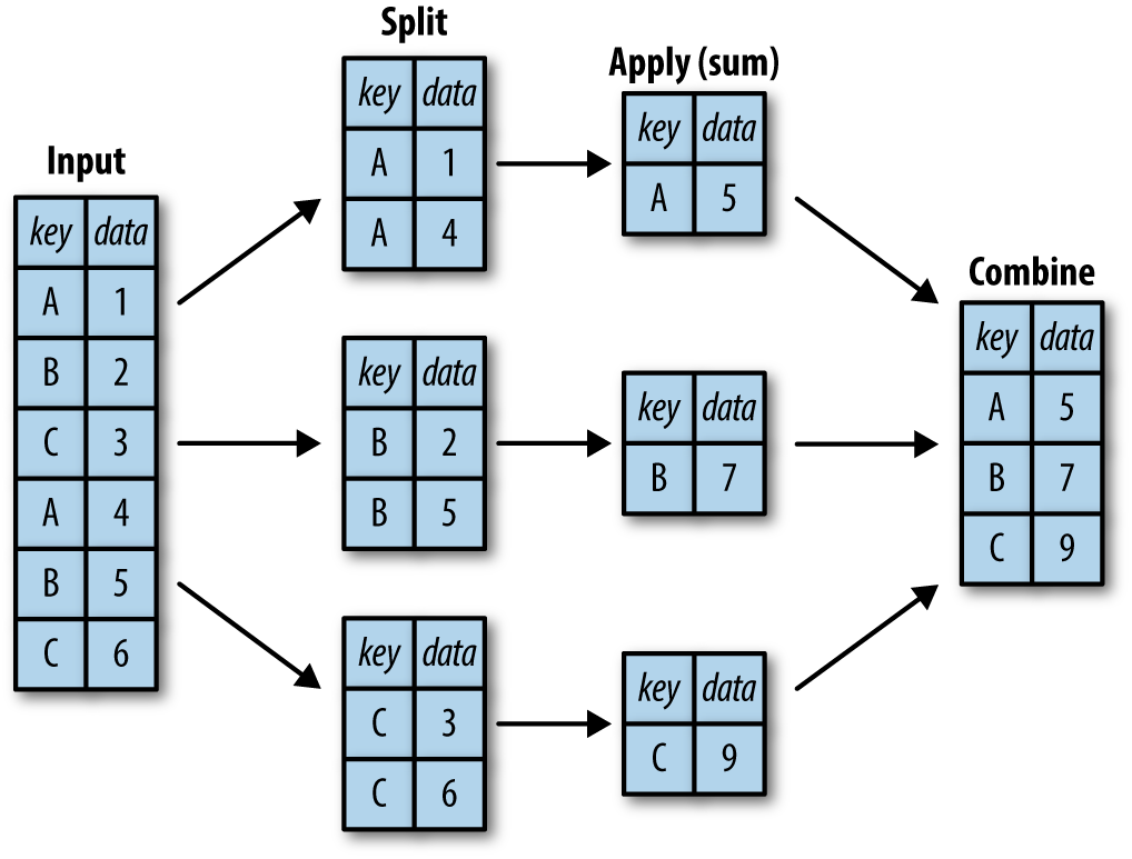
Figure 3-1. A visual representation of a groupby operation
While we could certainly do this manually using some combination of
the masking, aggregation, and merging commands covered earlier, it’s
important to realize that the intermediate splits do not need to be
explicitly instantiated. Rather, the GroupBy can (often) do this in a
single pass over the data, updating the sum, mean, count, min, or other
aggregate for each group along the way. The power of the GroupBy is that
it abstracts away these steps: the user need not think about how the
computation is done under the hood, but rather thinks about the
operation as a whole.
As a concrete example, let’s take a look at using Pandas for the computation
shown in Figure 3-1. We’ll start by creating the input DataFrame:
In[11]:df=pd.DataFrame({'key':['A','B','C','A','B','C'],'data':range(6)},columns=['key','data'])df
Out[11]: key data
0 A 0
1 B 1
2 C 2
3 A 3
4 B 4
5 C 5
We can compute the most basic split-apply-combine operation with the
groupby() method of DataFrames, passing the name of the desired key
column:
In[12]:df.groupby('key')
Out[12]: <pandas.core.groupby.DataFrameGroupBy object at 0x117272160>
Notice that what is returned is not a set of DataFrames, but a
DataFrameGroupBy object. This object is where the magic is: you can
think of it as a special view of the DataFrame, which is poised to dig
into the groups but does no actual computation until the aggregation is
applied. This “lazy evaluation” approach means that common aggregates
can be implemented very efficiently in a way that is almost transparent
to the user.
To produce a result, we can apply an aggregate to this
DataFrameGroupBy object, which will perform the appropriate
apply/combine steps to produce the desired result:
In[13]:df.groupby('key').sum()
Out[13]: data
key
A 3
B 5
C 7
The sum() method is just one possibility here; you can apply virtually
any common Pandas or NumPy aggregation function, as well as virtually
any valid DataFrame operation, as we will see in the following discussion.
The GroupBy object
The GroupBy object is a very flexible abstraction. In many ways, you can
simply treat it as if it’s a collection of DataFrames, and it does the
difficult things under the hood. Let’s see some examples using the
Planets data.
Perhaps the most important operations made available by a GroupBy are
aggregate, filter, transform, and apply. We’ll discuss each of these more fully in “Aggregate, filter, transform, apply”, but before that let’s introduce some of
the other functionality that can be used with the basic GroupBy
operation.
Column indexing
The GroupBy object supports column indexing in the same way as the
DataFrame, and returns a modified GroupBy object. For example:
In[14]:planets.groupby('method')
Out[14]: <pandas.core.groupby.DataFrameGroupBy object at 0x1172727b8>
In[15]:planets.groupby('method')['orbital_period']
Out[15]: <pandas.core.groupby.SeriesGroupBy object at 0x117272da0>
Here we’ve selected a particular Series group from the original
DataFrame group by reference to its column name. As with the GroupBy
object, no computation is done until we call some aggregate on the
object:
In[16]:planets.groupby('method')['orbital_period'].median()
Out[16]: method
Astrometry 631.180000
Eclipse Timing Variations 4343.500000
Imaging 27500.000000
Microlensing 3300.000000
Orbital Brightness Modulation 0.342887
Pulsar Timing 66.541900
Pulsation Timing Variations 1170.000000
Radial Velocity 360.200000
Transit 5.714932
Transit Timing Variations 57.011000
Name: orbital_period, dtype: float64
This gives an idea of the general scale of orbital periods (in days) that each method is sensitive to.
Iteration over groups
The GroupBy object supports direct iteration over the groups, returning
each group as a Series or DataFrame:
In[17]:for(method,group)inplanets.groupby('method'):("{0:30s} shape={1}".format(method,group.shape))
Astrometry shape=(2, 6) Eclipse Timing Variations shape=(9, 6) Imaging shape=(38, 6) Microlensing shape=(23, 6) Orbital Brightness Modulation shape=(3, 6) Pulsar Timing shape=(5, 6) Pulsation Timing Variations shape=(1, 6) Radial Velocity shape=(553, 6) Transit shape=(397, 6) Transit Timing Variations shape=(4, 6)
This can be useful for doing certain things manually, though it is often
much faster to use the built-in apply functionality, which we will
discuss momentarily.
Dispatch methods
Through some Python class magic, any method not explicitly implemented
by the GroupBy object will be passed through and called on the groups,
whether they are DataFrame or Series objects. For example, you can use
the describe() method of DataFrames to perform a set of aggregations
that describe each group in the data:
In[18]:planets.groupby('method')['year'].describe().unstack()
Out[18]:
count mean std min 25% \\
method
Astrometry 2.0 2011.500000 2.121320 2010.0 2010.75
Eclipse Timing Variations 9.0 2010.000000 1.414214 2008.0 2009.00
Imaging 38.0 2009.131579 2.781901 2004.0 2008.00
Microlensing 23.0 2009.782609 2.859697 2004.0 2008.00
Orbital Brightness Modulation 3.0 2011.666667 1.154701 2011.0 2011.00
Pulsar Timing 5.0 1998.400000 8.384510 1992.0 1992.00
Pulsation Timing Variations 1.0 2007.000000 NaN 2007.0 2007.00
Radial Velocity 553.0 2007.518987 4.249052 1989.0 2005.00
Transit 397.0 2011.236776 2.077867 2002.0 2010.00
Transit Timing Variations 4.0 2012.500000 1.290994 2011.0 2011.75
50% 75% max
method
Astrometry 2011.5 2012.25 2013.0
Eclipse Timing Variations 2010.0 2011.00 2012.0
Imaging 2009.0 2011.00 2013.0
Microlensing 2010.0 2012.00 2013.0
Orbital Brightness Modulation 2011.0 2012.00 2013.0
Pulsar Timing 1994.0 2003.00 2011.0
Pulsation Timing Variations 2007.0 2007.00 2007.0
Radial Velocity 2009.0 2011.00 2014.0
Transit 2012.0 2013.00 2014.0
Transit Timing Variations 2012.5 2013.25 2014.0
Looking at this table helps us to better understand the data: for example, the vast majority of planets have been discovered by the Radial Velocity and Transit methods, though the latter only became common (due to new, more accurate telescopes) in the last decade. The newest methods seem to be Transit Timing Variation and Orbital Brightness Modulation, which were not used to discover a new planet until 2011.
This is just one example of the utility of dispatch methods. Notice that
they are applied to each individual group, and the results are then
combined within GroupBy and returned. Again, any valid DataFrame/Series
method can be used on the corresponding GroupBy object, which allows for
some very flexible and powerful operations!
Aggregate, filter, transform, apply
The preceding discussion focused on aggregation for the combine operation,
but there are more options available. In particular, GroupBy objects
have aggregate(), filter(), transform(), and apply() methods
that efficiently implement a variety of useful operations before
combining the grouped data.
For the purpose of the following subsections, we’ll use this
DataFrame:
In[19]:rng=np.random.RandomState(0)df=pd.DataFrame({'key':['A','B','C','A','B','C'],'data1':range(6),'data2':rng.randint(0,10,6)},columns=['key','data1','data2'])df
Out[19]: key data1 data2
0 A 0 5
1 B 1 0
2 C 2 3
3 A 3 3
4 B 4 7
5 C 5 9
Aggregation
We’re now familiar with GroupBy aggregations with sum(), median(),
and the like, but the aggregate() method allows for even more flexibility. It
can take a string, a function, or a list thereof, and compute all the
aggregates at once. Here is a quick example combining all these:
In[20]:df.groupby('key').aggregate(['min',np.median,max])
Out[20]: data1 data2
min median max min median max
key
A 0 1.5 3 3 4.0 5
B 1 2.5 4 0 3.5 7
C 2 3.5 5 3 6.0 9
Another useful pattern is to pass a dictionary mapping column names to operations to be applied on that column:
In[21]:df.groupby('key').aggregate({'data1':'min','data2':'max'})
Out[21]: data1 data2
key
A 0 5
B 1 7
C 2 9
Filtering
A filtering operation allows you to drop data based on the group properties. For example, we might want to keep all groups in which the standard deviation is larger than some critical value:
In[22]:deffilter_func(x):returnx['data2'].std()>4(df);(df.groupby('key').std());(df.groupby('key').filter(filter_func))
df df.groupby('key').std()
key data1 data2 key data1 data2
0 A 0 5 A 2.12132 1.414214
1 B 1 0 B 2.12132 4.949747
2 C 2 3 C 2.12132 4.242641
3 A 3 3
4 B 4 7
5 C 5 9
df.groupby('key').filter(filter_func)
key data1 data2
1 B 1 0
2 C 2 3
4 B 4 7
5 C 5 9
The filter() function should return a Boolean value specifying whether the
group passes the filtering. Here because group A does not have a
standard deviation greater than 4, it is dropped from the result.
Transformation
While aggregation must return a reduced version of the data, transformation can return some transformed version of the full data to recombine. For such a transformation, the output is the same shape as the input. A common example is to center the data by subtracting the group-wise mean:
In[23]:df.groupby('key').transform(lambdax:x-x.mean())
Out[23]: data1 data2
0 -1.5 1.0
1 -1.5 -3.5
2 -1.5 -3.0
3 1.5 -1.0
4 1.5 3.5
5 1.5 3.0
The apply() method
The apply() method lets you apply an arbitrary function to the group
results. The function should take a DataFrame, and return either a
Pandas object (e.g., DataFrame, Series) or a scalar; the combine
operation will be tailored to the type of output returned.
For example, here is an apply() that normalizes the first column by
the sum of the second:
In[24]:defnorm_by_data2(x):# x is a DataFrame of group valuesx['data1']/=x['data2'].sum()returnx(df);(df.groupby('key').apply(norm_by_data2))
df df.groupby('key').apply(norm_by_data2)
key data1 data2 key data1 data2
0 A 0 5 0 A 0.000000 5
1 B 1 0 1 B 0.142857 0
2 C 2 3 2 C 0.166667 3
3 A 3 3 3 A 0.375000 3
4 B 4 7 4 B 0.571429 7
5 C 5 9 5 C 0.416667 9
apply() within a GroupBy is quite flexible: the only criterion is that
the function takes a DataFrame and returns a Pandas object or scalar;
what you do in the middle is up to you!
Specifying the split key
In the simple examples presented before, we split the DataFrame on a single
column name. This is just one of many options by which the groups can be
defined, and we’ll go through some other options for group specification
here.
A list, array, series, or index providing the grouping keys
The key can be any series or list with a length matching that of the
DataFrame. For example:
In[25]:L=[0,1,0,1,2,0](df);(df.groupby(L).sum())
df df.groupby(L).sum() key data1 data2 data1 data2 0 A 0 5 0 7 17 1 B 1 0 1 4 3 2 C 2 3 2 4 7 3 A 3 3 4 B 4 7 5 C 5 9
Of course, this means there’s another, more verbose way of accomplishing
the df.groupby('key') from before:
In[26]:(df);(df.groupby(df['key']).sum())
df df.groupby(df['key']).sum() key data1 data2 data1 data2 0 A 0 5 A 3 8 1 B 1 0 B 5 7 2 C 2 3 C 7 12 3 A 3 3 4 B 4 7 5 C 5 9
A dictionary or series mapping index to group
Another method is to provide a dictionary that maps index values to the group keys:
In[27]:df2=df.set_index('key')mapping={'A':'vowel','B':'consonant','C':'consonant'}(df2);(df2.groupby(mapping).sum())
df2 df2.groupby(mapping).sum() key data1 data2 data1 data2 A 0 5 consonant 12 19 B 1 0 vowel 3 8 C 2 3 A 3 3 B 4 7 C 5 9
Any Python function
Similar to mapping, you can pass any Python function that will input the index value and output the group:
In[28]:(df2);(df2.groupby(str.lower).mean())
df2 df2.groupby(str.lower).mean() key data1 data2 data1 data2 A 0 5 a 1.5 4.0 B 1 0 b 2.5 3.5 C 2 3 c 3.5 6.0 A 3 3 B 4 7 C 5 9
A list of valid keys
Further, any of the preceding key choices can be combined to group on a multi-index:
In[29]:df2.groupby([str.lower,mapping]).mean()
Out[29]: data1 data2
a vowel 1.5 4.0
b consonant 2.5 3.5
c consonant 3.5 6.0
Grouping example
As an example of this, in a couple lines of Python code we can put all these together and count discovered planets by method and by decade:
In[30]:decade=10*(planets['year']//10)decade=decade.astype(str)+'s'decade.name='decade'planets.groupby(['method',decade])['number'].sum().unstack().fillna(0)
Out[30]: decade 1980s 1990s 2000s 2010s
method
Astrometry 0.0 0.0 0.0 2.0
Eclipse Timing Variations 0.0 0.0 5.0 10.0
Imaging 0.0 0.0 29.0 21.0
Microlensing 0.0 0.0 12.0 15.0
Orbital Brightness Modulation 0.0 0.0 0.0 5.0
Pulsar Timing 0.0 9.0 1.0 1.0
Pulsation Timing Variations 0.0 0.0 1.0 0.0
Radial Velocity 1.0 52.0 475.0 424.0
Transit 0.0 0.0 64.0 712.0
Transit Timing Variations 0.0 0.0 0.0 9.0
This shows the power of combining many of the operations we’ve discussed up to this point when looking at realistic datasets. We immediately gain a coarse understanding of when and how planets have been discovered over the past several decades!
Here I would suggest digging into these few lines of code, and evaluating the individual steps to make sure you understand exactly what they are doing to the result. It’s certainly a somewhat complicated example, but understanding these pieces will give you the means to similarly explore your own data.
Pivot Tables
We have seen how the GroupBy abstraction lets us explore relationships
within a dataset. A pivot table is a similar operation that is
commonly seen in spreadsheets and other programs that operate on
tabular data. The pivot table takes simple column-wise data as input,
and groups the entries into a two-dimensional table that provides a
multidimensional summarization of the data. The difference between
pivot tables and GroupBy can sometimes cause confusion; it helps me to
think of pivot tables as essentially a multidimensional version of
GroupBy aggregation. That is, you split-apply-combine, but both the
split and the combine happen across not a one-dimensional index, but
across a two-dimensional grid.
Motivating Pivot Tables
For the examples in this section, we’ll use the database of passengers on the Titanic, available through the Seaborn library (see “Visualization with Seaborn”):
In[1]:importnumpyasnpimportpandasaspdimportseabornassnstitanic=sns.load_dataset('titanic')
In[2]:titanic.head()
Out[2]:
survived pclass sex age sibsp parch fare embarked class \\
0 0 3 male 22.0 1 0 7.2500 S Third
1 1 1 female 38.0 1 0 71.2833 C First
2 1 3 female 26.0 0 0 7.9250 S Third
3 1 1 female 35.0 1 0 53.1000 S First
4 0 3 male 35.0 0 0 8.0500 S Third
who adult_male deck embark_town alive alone
0 man True NaN Southampton no False
1 woman False C Cherbourg yes False
2 woman False NaN Southampton yes True
3 woman False C Southampton yes False
4 man True NaN Southampton no True
This contains a wealth of information on each passenger of that ill-fated voyage, including gender, age, class, fare paid, and much more.
Pivot Tables by Hand
To start learning more about this data, we might begin by grouping it according to gender, survival status, or some combination thereof. If you have
read the previous section, you might be tempted to apply a GroupBy
operation—for example, let’s look at survival rate by gender:
In[3]:titanic.groupby('sex')[['survived']].mean()
Out[3]: survived
sex
female 0.742038
male 0.188908
This immediately gives us some insight: overall, three of every four females on board survived, while only one in five males survived!
This is useful, but we might like to go one step deeper and look at
survival by both sex and, say, class. Using the vocabulary of GroupBy,
we might proceed using something like this: we group by class and gender,
select survival, apply a mean aggregate, combine the resulting
groups, and then unstack the hierarchical index to reveal the hidden
multidimensionality. In code:
In[4]:titanic.groupby(['sex','class'])['survived'].aggregate('mean').unstack()
Out[4]: class First Second Third
sex
female 0.968085 0.921053 0.500000
male 0.368852 0.157407 0.135447
This gives us a better idea of how both gender and class affected
survival, but the code is starting to look a bit garbled. While each
step of this pipeline makes sense in light of the tools we’ve previously
discussed, the long string of code is not particularly easy to read or
use. This two-dimensional GroupBy is common enough that Pandas includes
a convenience routine, pivot_table, which succinctly handles this type
of multidimensional aggregation.
Pivot Table Syntax
Here is the equivalent to the preceding operation using the pivot_table
method of DataFrames:
In[5]:titanic.pivot_table('survived',index='sex',columns='class')
Out[5]: class First Second Third
sex
female 0.968085 0.921053 0.500000
male 0.368852 0.157407 0.135447
This is eminently more readable than the GroupBy approach, and produces
the same result. As you might expect of an early 20th-century
transatlantic cruise, the survival gradient favors both women and higher
classes. First-class women survived with near certainty (hi, Rose!),
while only one in ten third-class men survived (sorry, Jack!).
Multilevel pivot tables
Just as in the GroupBy, the grouping in pivot tables can be specified
with multiple levels, and via a number of options. For example, we might
be interested in looking at age as a third dimension. We’ll bin the age
using the pd.cut function:
In[6]:age=pd.cut(titanic['age'],[0,18,80])titanic.pivot_table('survived',['sex',age],'class')
Out[6]: class First Second Third
sex age
female (0, 18] 0.909091 1.000000 0.511628
(18, 80] 0.972973 0.900000 0.423729
male (0, 18] 0.800000 0.600000 0.215686
(18, 80] 0.375000 0.071429 0.133663
We can apply this same strategy when working with the columns as well; let’s add info on the fare
paid using pd.qcut to automatically compute quantiles:
In[7]:fare=pd.qcut(titanic['fare'],2)titanic.pivot_table('survived',['sex',age],[fare,'class'])
Out[7]:
fare [0, 14.454]
class First Second Third \\
sex age
female (0, 18] NaN 1.000000 0.714286
(18, 80] NaN 0.880000 0.444444
male (0, 18] NaN 0.000000 0.260870
(18, 80] 0.0 0.098039 0.125000
fare (14.454, 512.329]
class First Second Third
sex age
female (0, 18] 0.909091 1.000000 0.318182
(18, 80] 0.972973 0.914286 0.391304
male (0, 18] 0.800000 0.818182 0.178571
(18, 80] 0.391304 0.030303 0.192308
The result is a four-dimensional aggregation with hierarchical indices (see “Hierarchical Indexing”), shown in a grid demonstrating the relationship between the values.
Additional pivot table options
The full call signature of the pivot_table method of DataFrames is as
follows:
# call signature as of Pandas 0.18DataFrame.pivot_table(data,values=None,index=None,columns=None,aggfunc='mean',fill_value=None,margins=False,dropna=True,margins_name='All')
We’ve already seen examples of the first three arguments; here we’ll take
a quick look at the remaining ones. Two of the options,
fill_value and dropna, have to do with missing data and are fairly
straightforward; we will not show examples of them here.
The aggfunc keyword controls what type of aggregation is applied,
which is a mean by default. As in the GroupBy, the aggregation
specification can be a string representing one of several common choices
('sum', 'mean', 'count', 'min', 'max', etc.) or a
function that implements an aggregation (np.sum(), min(),
sum(), etc.). Additionally, it can be specified as a dictionary mapping
a column to any of the above desired options:
In[8]:titanic.pivot_table(index='sex',columns='class',aggfunc={'survived':sum,'fare':'mean'})
Out[8]: fare survived
class First Second Third First Second Third
sex
female 106.125798 21.970121 16.118810 91.0 70.0 72.0
male 67.226127 19.741782 12.661633 45.0 17.0 47.0
Notice also here that we’ve omitted the values keyword; when you’re specifying a mapping for aggfunc, this is determined automatically.
At times it’s useful to compute totals along each grouping. This can be
done via the margins keyword:
In[9]:titanic.pivot_table('survived',index='sex',columns='class',margins=True)
Out[9]: class First Second Third All
sex
female 0.968085 0.921053 0.500000 0.742038
male 0.368852 0.157407 0.135447 0.188908
All 0.629630 0.472826 0.242363 0.383838
Here this automatically gives us information about the class-agnostic
survival rate by gender, the gender-agnostic survival rate by class, and
the overall survival rate of 38%. The margin label can be specified with
the margins_name keyword, which defaults to "All".
Example: Birthrate Data
As a more interesting example, let’s take a look at the freely available data on births in the United States, provided by the Centers for Disease Control (CDC). This data can be found at https://raw.githubusercontent.com/jakevdp/data-CDCbirths/master/births.csv (this dataset has been analyzed rather extensively by Andrew Gelman and his group; see, for example, this blog post):
In[10]:# shell command to download the data:# !curl -O https://raw.githubusercontent.com/jakevdp/data-CDCbirths/# master/births.csv
In[11]:births=pd.read_csv('births.csv')
Taking a look at the data, we see that it’s relatively simple—it contains the number of births grouped by date and gender:
In[12]:births.head()
Out[12]: year month day gender births
0 1969 1 1 F 4046
1 1969 1 1 M 4440
2 1969 1 2 F 4454
3 1969 1 2 M 4548
4 1969 1 3 F 4548
We can start to understand this data a bit more by using a pivot table. Let’s add a decade column, and take a look at male and female births as a function of decade:
In[13]:births['decade']=10*(births['year']//10)births.pivot_table('births',index='decade',columns='gender',aggfunc='sum')
Out[13]: gender F M
decade
1960 1753634 1846572
1970 16263075 17121550
1980 18310351 19243452
1990 19479454 20420553
2000 18229309 19106428
We immediately see that male births outnumber female births in every decade. To see this trend a bit more clearly, we can use the built-in plotting tools in Pandas to visualize the total number of births by year (Figure 3-2; see Chapter 4 for a discussion of plotting with Matplotlib):
In[14]:%matplotlibinlineimportmatplotlib.pyplotaspltsns.set()# use Seaborn stylesbirths.pivot_table('births',index='year',columns='gender',aggfunc='sum').plot()plt.ylabel('total births per year');
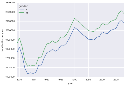
Figure 3-2. Total number of US births by year and gender
With a simple pivot table and plot() method, we can immediately see
the annual trend in births by gender. By eye, it appears that over the
past 50 years male births have outnumbered female births by around 5%.
Further data exploration
Though this doesn’t necessarily relate to the pivot table, there are a few more interesting features we can pull out of this dataset using the Pandas tools covered up to this point. We must start by cleaning the data a bit, removing outliers caused by mistyped dates (e.g., June 31st) or missing values (e.g., June 99th). One easy way to remove these all at once is to cut outliers; we’ll do this via a robust sigma-clipping operation:1
In[15]:quartiles=np.percentile(births['births'],[25,50,75])mu=quartiles[1]sig=0.74*(quartiles[2]-quartiles[0])
This final line is a robust estimate of the sample mean, where the 0.74
comes from the interquartile range of a Gaussian distribution. With this
we can use the query() method (discussed further in
“High-Performance Pandas: eval() and query()”) to filter out rows with births outside these
values:
In[16]:births=births.query('(births > @mu - 5 * @sig) & (births < @mu + 5 * @sig)')
Next we set the day column to integers; previously it had been a
string because some columns in the dataset contained the value 'null':
In[17]:# set 'day' column to integer; it originally was a string due to nullsbirths['day']=births['day'].astype(int)
Finally, we can combine the day, month, and year to create a Date index (see “Working with Time Series”). This allows us to quickly compute the weekday corresponding to each row:
In[18]:# create a datetime index from the year, month, daybirths.index=pd.to_datetime(10000*births.year+100*births.month+births.day,format='%Y%m%d')births['dayofweek']=births.index.dayofweek
Using this we can plot births by weekday for several decades (Figure 3-3):
In[19]:importmatplotlib.pyplotaspltimportmatplotlibasmplbirths.pivot_table('births',index='dayofweek',columns='decade',aggfunc='mean').plot()plt.gca().set_xticklabels(['Mon','Tues','Wed','Thurs','Fri','Sat','Sun'])plt.ylabel('mean births by day');
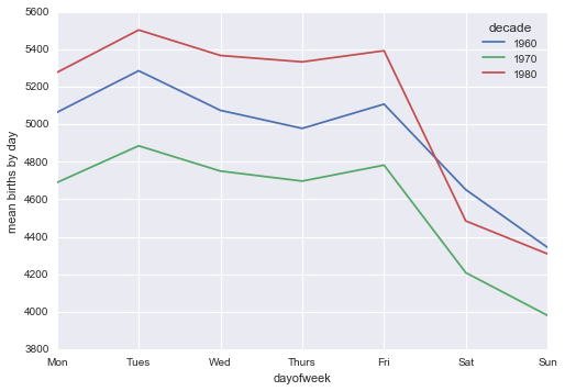
Figure 3-3. Average daily births by day of week and decade
Apparently births are slightly less common on weekends than on weekdays! Note that the 1990s and 2000s are missing because the CDC data contains only the month of birth starting in 1989.
Another interesting view is to plot the mean number of births by the day of the year. Let’s first group the data by month and day separately:
In[20]:births_by_date=births.pivot_table('births',[births.index.month,births.index.day])births_by_date.head()
Out[20]: 1 1 4009.225
2 4247.400
3 4500.900
4 4571.350
5 4603.625
Name: births, dtype: float64
The result is a multi-index over months and days. To make this easily plottable, let’s turn these months and days into a date by associating them with a dummy year variable (making sure to choose a leap year so February 29th is correctly handled!)
In[21]:births_by_date.index=[pd.datetime(2012,month,day)for(month,day)inbirths_by_date.index]births_by_date.head()
Out[21]: 2012-01-01 4009.225
2012-01-02 4247.400
2012-01-03 4500.900
2012-01-04 4571.350
2012-01-05 4603.625
Name: births, dtype: float64
Focusing on the month and day only, we now have a time series reflecting
the average number of births by date of the year. From this, we can use
the plot method to plot the data (Figure 3-4). It reveals some interesting trends:
In[22]:# Plot the resultsfig,ax=plt.subplots(figsize=(12,4))births_by_date.plot(ax=ax);
Figure 3-4. Average daily births by date
In particular, the striking feature of this graph is the dip in birthrate on US holidays (e.g., Independence Day, Labor Day, Thanksgiving, Christmas, New Year’s Day) although this likely reflects trends in scheduled/induced births rather than some deep psychosomatic effect on natural births. For more discussion on this trend, see the analysis and links in Andrew Gelman’s blog post on the subject. We’ll return to this figure in “Example: Effect of Holidays on US Births”, where we will use Matplotlib’s tools to annotate this plot.
Looking at this short example, you can see that many of the Python and Pandas tools we’ve seen to this point can be combined and used to gain insight from a variety of datasets. We will see some more sophisticated applications of these data manipulations in future sections!
Vectorized String Operations
One strength of Python is its relative ease in handling and manipulating string data. Pandas builds on this and provides a comprehensive set of vectorized string operations that become an essential piece of the type of munging required when one is working with (read: cleaning up) real-world data. In this section, we’ll walk through some of the Pandas string operations, and then take a look at using them to partially clean up a very messy dataset of recipes collected from the Internet.
Introducing Pandas String Operations
We saw in previous sections how tools like NumPy and Pandas generalize arithmetic operations so that we can easily and quickly perform the same operation on many array elements. For example:
In[1]:importnumpyasnpx=np.array([2,3,5,7,11,13])x*2
Out[1]: array([ 4, 6, 10, 14, 22, 26])
This vectorization of operations simplifies the syntax of operating on arrays of data: we no longer have to worry about the size or shape of the array, but just about what operation we want done. For arrays of strings, NumPy does not provide such simple access, and thus you’re stuck using a more verbose loop syntax:
In[2]:data=['peter','Paul','MARY','gUIDO'][s.capitalize()forsindata]
Out[2]: ['Peter', 'Paul', 'Mary', 'Guido']
This is perhaps sufficient to work with some data, but it will break if there are any missing values. For example:
In[3]:data=['peter','Paul',None,'MARY','gUIDO'][s.capitalize()forsindata]
---------------------------------------------------------------------------
---------------------------------------------------------------------------
AttributeError Traceback (most recent call last)
<ipython-input-3-fc1d891ab539> in <module>()
1 data = ['peter', 'Paul', None, 'MARY', 'gUIDO']
----> 2 [s.capitalize() for s in data]
<ipython-input-3-fc1d891ab539> in <listcomp>(.0)
1 data = ['peter', 'Paul', None, 'MARY', 'gUIDO']
----> 2 [s.capitalize() for s in data]
AttributeError: 'NoneType' object has no attribute 'capitalize'
---------------------------------------------------------------------------
Pandas includes features to address both this need for vectorized string
operations and for correctly handling missing data via the str
attribute of Pandas Series and Index objects containing strings. So, for
example, suppose we create a Pandas Series with this data:
In[4]:importpandasaspdnames=pd.Series(data)names
Out[4]: 0 peter
1 Paul
2 None
3 MARY
4 gUIDO
dtype: object
We can now call a single method that will capitalize all the entries, while skipping over any missing values:
In[5]:names.str.capitalize()
Out[5]: 0 Peter
1 Paul
2 None
3 Mary
4 Guido
dtype: object
Using tab completion on this str attribute will list all the
vectorized string methods available to Pandas.
Tables of Pandas String Methods
If you have a good understanding of string manipulation in Python, most of Pandas’ string syntax is intuitive enough that it’s probably sufficient to just list a table of available methods; we will start with that here, before diving deeper into a few of the subtleties. The examples in this section use the following series of names:
In[6]:monte=pd.Series(['Graham Chapman','John Cleese','Terry Gilliam','Eric Idle','Terry Jones','Michael Palin'])
Methods similar to Python string methods
Nearly all Python’s built-in string methods are mirrored by a Pandas
vectorized string method. Here is a list of Pandas str methods that
mirror Python string methods:
|
|
|
|
|
|
|
|
|
|
|
|
|
|
|
|
|
|
|
|
|
|
|
|
|
|
|
|
|
|
|
|
Notice that these have various return values. Some, like lower(), return a series of strings:
In[7]:monte.str.lower()
Out[7]: 0 graham chapman
1 john cleese
2 terry gilliam
3 eric idle
4 terry jones
5 michael palin
dtype: object
But some others return numbers:
In[8]:monte.str.len()
Out[8]: 0 14
1 11
2 13
3 9
4 11
5 13
dtype: int64
Or Boolean values:
In[9]:monte.str.startswith('T')
Out[9]: 0 False
1 False
2 True
3 False
4 True
5 False
dtype: bool
Still others return lists or other compound values for each element:
In[10]:monte.str.split()
Out[10]: 0 [Graham, Chapman]
1 [John, Cleese]
2 [Terry, Gilliam]
3 [Eric, Idle]
4 [Terry, Jones]
5 [Michael, Palin]
dtype: object
We’ll see further manipulations of this kind of series-of-lists object as we continue our discussion.
Methods using regular expressions
In addition, there are several methods that accept regular expressions
to examine the content of each string element, and follow some of the
API conventions of Python’s built-in re module (see Table 3-4).
| Method | Description |
|---|---|
|
Call |
|
Call |
|
Call |
|
Replace occurrences of pattern with some other string. |
|
Call |
|
Count occurrences of pattern. |
|
Equivalent to |
|
Equivalent to |
With these, you can do a wide range of interesting operations. For example, we can extract the first name from each by asking for a contiguous group of characters at the beginning of each element:
In[11]:monte.str.extract('([A-Za-z]+)')
Out[11]: 0 Graham
1 John
2 Terry
3 Eric
4 Terry
5 Michael
dtype: object
Or we can do something more complicated, like finding all names that
start and end with a consonant, making use of the start-of-string
(^) and end-of-string ($) regular expression characters:
In[12]:monte.str.findall(r'^[^AEIOU].*[^aeiou]$')
Out[12]: 0 [Graham Chapman]
1 []
2 [Terry Gilliam]
3 []
4 [Terry Jones]
5 [Michael Palin]
dtype: object
The ability to concisely apply regular expressions across Series or
DataFrame entries opens up many possibilities for analysis and cleaning
of data.
Miscellaneous methods
Finally, there are some miscellaneous methods that enable other convenient operations (see Table 3-5).
| Method | Description |
|---|---|
|
Index each element |
|
Slice each element |
|
Replace slice in each element with passed value |
|
Concatenate strings |
|
Repeat values |
|
Return Unicode form of string |
|
Add whitespace to left, right, or both sides of strings |
|
Split long strings into lines with length less than a given width |
|
Join strings in each element of the |
|
Extract dummy variables as a |
Vectorized item access and slicing
The get() and slice() operations, in particular, enable vectorized
element access from each array. For example, we can get a slice of the
first three characters of each array using str.slice(0, 3). Note that
this behavior is also available through Python’s normal indexing syntax—for example, df.str.slice(0, 3) is equivalent to df.str[0:3]:
In[13]:monte.str[0:3]
Out[13]: 0 Gra
1 Joh
2 Ter
3 Eri
4 Ter
5 Mic
dtype: object
Indexing via df.str.get(i) and df.str[i] is similar.
These get() and slice() methods also let you access elements of
arrays returned by split(). For example, to extract the last
name of each entry, we can combine split() and get():
In[14]:monte.str.split().str.get(-1)
Out[14]: 0 Chapman
1 Cleese
2 Gilliam
3 Idle
4 Jones
5 Palin
dtype: object
Indicator variables
Another method that requires a bit of extra explanation is the
get_dummies() method. This is useful when your data has a column
containing some sort of coded indicator. For example, we might have a
dataset that contains information in the form of codes, such as A=“born
in America,” B=“born in the United Kingdom,” C=“likes cheese,” D=“likes
spam”:
In[15]:full_monte=pd.DataFrame({'name':monte,'info':['B|C|D','B|D','A|C','B|D','B|C','B|C|D']})full_monte
Out[15]: info name
0 B|C|D Graham Chapman
1 B|D John Cleese
2 A|C Terry Gilliam
3 B|D Eric Idle
4 B|C Terry Jones
5 B|C|D Michael Palin
The get_dummies() routine lets you quickly split out these indicator
variables into a DataFrame:
In[16]:full_monte['info'].str.get_dummies('|')
Out[16]: A B C D
0 0 1 1 1
1 0 1 0 1
2 1 0 1 0
3 0 1 0 1
4 0 1 1 0
5 0 1 1 1
With these operations as building blocks, you can construct an endless range of string processing procedures when cleaning your data.
We won’t dive further into these methods here, but I encourage you to
read through “Working with Text Data” in the pandas online documentation, or to refer to the resources listed in
“Further Resources”.
Example: Recipe Database
These vectorized string operations become most useful in the process of cleaning up messy, real-world data. Here I’ll walk through an example of that, using an open recipe database compiled from various sources on the Web. Our goal will be to parse the recipe data into ingredient lists, so we can quickly find a recipe based on some ingredients we have on hand.
The scripts used to compile this can be found at https://github.com/fictivekin/openrecipes, and the link to the current version of the database is found there as well.
As of spring 2016, this database is about 30 MB, and can be downloaded and unzipped with these commands:
In[17]:# !curl -O http://openrecipes.s3.amazonaws.com/recipeitems-latest.json.gz# !gunzip recipeitems-latest.json.gz
The database is in JSON format, so we will try pd.read_json to read it:
In[18]:try:recipes=pd.read_json('recipeitems-latest.json')exceptValueErrorase:("ValueError:",e)
ValueError: Trailing data
Oops! We get a ValueError mentioning that there is “trailing data.”
Searching for this error on the Internet, it seems that it’s due to
using a file in which each line is itself a valid JSON, but the full
file is not. Let’s check if this interpretation is true:
In[19]:withopen('recipeitems-latest.json')asf:line=f.readline()pd.read_json(line).shape
Out[19]: (2, 12)
Yes, apparently each line is a valid JSON, so we’ll need to string them
together. One way we can do this is to actually construct a string
representation containing all these JSON entries, and then load the
whole thing with pd.read_json:
In[20]:# read the entire file into a Python arraywithopen('recipeitems-latest.json','r')asf:# Extract each linedata=(line.strip()forlineinf)# Reformat so each line is the element of a listdata_json="[{0}]".format(','.join(data))# read the result as a JSONrecipes=pd.read_json(data_json)
In[21]:recipes.shape
Out[21]: (173278, 17)
We see there are nearly 200,000 recipes, and 17 columns. Let’s take a look at one row to see what we have:
In[22]:recipes.iloc[0]
Out[22]:
_id {'$oid': '5160756b96cc62079cc2db15'}
cookTime PT30M
creator NaN
dateModified NaN
datePublished 2013-03-11
description Late Saturday afternoon, after Marlboro Man ha...
image http://static.thepioneerwoman.com/cooking/file...
ingredients Biscuits\n3 cups All-purpose Flour\n2 Tablespo...
name Drop Biscuits and Sausage Gravy
prepTime PT10M
recipeCategory NaN
recipeInstructions NaN
recipeYield 12
source thepioneerwoman
totalTime NaN
ts {'$date': 1365276011104}
url http://thepioneerwoman.com/cooking/2013/03/dro...
Name: 0, dtype: object
There is a lot of information there, but much of it is in a very messy form, as is typical of data scraped from the Web. In particular, the ingredient list is in string format; we’re going to have to carefully extract the information we’re interested in. Let’s start by taking a closer look at the ingredients:
In[23]:recipes.ingredients.str.len().describe()
Out[23]: count 173278.000000
mean 244.617926
std 146.705285
min 0.000000
25% 147.000000
50% 221.000000
75% 314.000000
max 9067.000000
Name: ingredients, dtype: float64
The ingredient lists average 250 characters long, with a minimum of 0 and a maximum of nearly 10,000 characters!
Just out of curiosity, let’s see which recipe has the longest ingredient list:
In[24]:recipes.name[np.argmax(recipes.ingredients.str.len())]
Out[24]: 'Carrot Pineapple Spice & Brownie Layer Cake with Whipped Cream & Cream Cheese Frosting and Marzipan Carrots'
That certainly looks like an involved recipe.
We can do other aggregate explorations; for example, let’s see how many of the recipes are for breakfast food:
In[33]:recipes.description.str.contains('[Bb]reakfast').sum()
Out[33]: 3524
Or how many of the recipes list cinnamon as an ingredient:
In[34]:recipes.ingredients.str.contains('[Cc]innamon').sum()
Out[34]: 10526
We could even look to see whether any recipes misspell the ingredient as “cinamon”:
In[27]:recipes.ingredients.str.contains('[Cc]inamon').sum()
Out[27]: 11
This is the type of essential data exploration that is possible with Pandas string tools. It is data munging like this that Python really excels at.
A simple recipe recommender
Let’s go a bit further, and start working on a simple recipe recommendation system: given a list of ingredients, find a recipe that uses all those ingredients. While conceptually straightforward, the task is complicated by the heterogeneity of the data: there is no easy operation, for example, to extract a clean list of ingredients from each row. So we will cheat a bit: we’ll start with a list of common ingredients, and simply search to see whether they are in each recipe’s ingredient list. For simplicity, let’s just stick with herbs and spices for the time being:
In[28]:spice_list=['salt','pepper','oregano','sage','parsley','rosemary','tarragon','thyme','paprika','cumin']
We can then build a Boolean DataFrame consisting of True and False
values, indicating whether this ingredient appears in the list:
In[29]:importrespice_df=pd.DataFrame(dict((spice,recipes.ingredients.str.contains(spice,re.IGNORECASE))forspiceinspice_list))spice_df.head()
Out[29]: cumin oregano paprika parsley pepper rosemary sage salt tarragon thyme 0 False False False False False False True False False False 1 False False False False False False False False False False 2 True False False False True False False True False False 3 False False False False False False False False False False 4 False False False False False False False False False False
Now, as an example, let’s say we’d like to find a recipe that uses
parsley, paprika, and tarragon. We can compute this very quickly using
the query() method of DataFrames, discussed in
“High-Performance Pandas: eval() and query()”:
In[30]:selection=spice_df.query('parsley & paprika & tarragon')len(selection)
Out[30]: 10
We find only 10 recipes with this combination; let’s use the index returned by this selection to discover the names of the recipes that have this combination:
In[31]:recipes.name[selection.index]
Out[31]: 2069 All cremat with a Little Gem, dandelion and wa...
74964 Lobster with Thermidor butter
93768 Burton's Southern Fried Chicken with White Gravy
113926 Mijo's Slow Cooker Shredded Beef
137686 Asparagus Soup with Poached Eggs
140530 Fried Oyster Po’boys
158475 Lamb shank tagine with herb tabbouleh
158486 Southern fried chicken in buttermilk
163175 Fried Chicken Sliders with Pickles + Slaw
165243 Bar Tartine Cauliflower Salad
Name: name, dtype: object
Now that we have narrowed down our recipe selection by a factor of almost 20,000, we are in a position to make a more informed decision about what we’d like to cook for dinner.
Going further with recipes
Hopefully this example has given you a bit of a flavor (ba-dum!) for the types of data cleaning operations that are efficiently enabled by Pandas string methods. Of course, building a very robust recipe recommendation system would require a lot more work! Extracting full ingredient lists from each recipe would be an important piece of the task; unfortunately, the wide variety of formats used makes this a relatively time-consuming process. This points to the truism that in data science, cleaning and munging of real-world data often comprises the majority of the work, and Pandas provides the tools that can help you do this efficiently.
Working with Time Series
Pandas was developed in the context of financial modeling, so as you might expect, it contains a fairly extensive set of tools for working with dates, times, and time-indexed data. Date and time data comes in a few flavors, which we will discuss here:
-
Time stamps reference particular moments in time (e.g., July 4th, 2015, at 7:00 a.m.).
-
Time intervals and periods reference a length of time between a particular beginning and end point—for example, the year 2015. Periods usually reference a special case of time intervals in which each interval is of uniform length and does not overlap (e.g., 24 hour-long periods constituting days).
-
Time deltas or durations reference an exact length of time (e.g., a duration of 22.56 seconds).
In this section, we will introduce how to work with each of these types of date/time data in Pandas. This short section is by no means a complete guide to the time series tools available in Python or Pandas, but instead is intended as a broad overview of how you as a user should approach working with time series. We will start with a brief discussion of tools for dealing with dates and times in Python, before moving more specifically to a discussion of the tools provided by Pandas. After listing some resources that go into more depth, we will review some short examples of working with time series data in Pandas.
Dates and Times in Python
The Python world has a number of available representations of dates, times, deltas, and timespans. While the time series tools provided by Pandas tend to be the most useful for data science applications, it is helpful to see their relationship to other packages used in Python.
Native Python dates and times: datetime and dateutil
Python’s basic objects for working with dates and times reside in the
built-in datetime module. Along with the third-party dateutil
module, you can use it to quickly perform a host of useful
functionalities on dates and times. For example, you can manually build
a date using the datetime type:
In[1]:fromdatetimeimportdatetimedatetime(year=2015,month=7,day=4)
Out[1]: datetime.datetime(2015, 7, 4, 0, 0)
Or, using the dateutil module, you can parse dates from a variety of
string formats:
In[2]:fromdateutilimportparserdate=parser.parse("4th of July, 2015")date
Out[2]: datetime.datetime(2015, 7, 4, 0, 0)
Once you have a datetime object, you can do things like printing the
day of the week:
In[3]:date.strftime('%A')
Out[3]: 'Saturday'
In the final line, we’ve used one of the standard string format codes
for printing dates ("%A"), which you can read about in the
strftime
section of Python’s
datetime documentation.
Documentation of other useful date utilities can be found in
dateutil’s online documentation. A
related package to be aware of is pytz,
which contains tools for working with the most migraine-inducing piece of
time series data: time zones.
The power of datetime and dateutil lies in their flexibility and easy
syntax: you can use these objects and their built-in methods to easily
perform nearly any operation you might be interested in. Where they
break down is when you wish to work with large arrays of dates and
times: just as lists of Python numerical variables are suboptimal
compared to NumPy-style typed numerical arrays, lists of Python datetime
objects are suboptimal compared to typed arrays of encoded dates.
Typed arrays of times: NumPy’s datetime64
The weaknesses of Python’s datetime format inspired the NumPy team to
add a set of native time series data type to NumPy. The datetime64
dtype encodes dates as 64-bit integers, and thus allows arrays of dates
to be represented very compactly. The datetime64 requires a very
specific input format:
In[4]:importnumpyasnpdate=np.array('2015-07-04',dtype=np.datetime64)date
Out[4]: array(datetime.date(2015, 7, 4), dtype='datetime64[D]')
Once we have this date formatted, however, we can quickly do vectorized operations on it:
In[5]:date+np.arange(12)
Out[5]:
array(['2015-07-04', '2015-07-05', '2015-07-06', '2015-07-07',
'2015-07-08', '2015-07-09', '2015-07-10', '2015-07-11',
'2015-07-12', '2015-07-13', '2015-07-14', '2015-07-15'],
dtype='datetime64[D]')
Because of the uniform type in NumPy datetime64 arrays, this type of
operation can be accomplished much more quickly than if we were working
directly with Python’s datetime objects, especially as arrays get
large (we introduced this type of vectorization in
“Computation on NumPy Arrays: Universal Functions”).
One detail of the datetime64 and timedelta64 objects is that they
are built on a fundamental time unit. Because the datetime64 object
is limited to 64-bit precision, the range of encodable times is 264 times this fundamental unit. In other words,
datetime64 imposes a trade-off between time resolution and maximum
time span.
For example, if you want a time resolution of one nanosecond, you only have enough information to encode a range of 264 nanoseconds, or just under 600 years. NumPy will infer the desired unit from the input; for example, here is a day-based datetime:
In[6]:np.datetime64('2015-07-04')
Out[6]: numpy.datetime64('2015-07-04')
Here is a minute-based datetime:
In[7]:np.datetime64('2015-07-04 12:00')
Out[7]: numpy.datetime64('2015-07-04T12:00')
Notice that the time zone is automatically set to the local time on the computer executing the code. You can force any desired fundamental unit using one of many format codes; for example, here we’ll force a nanosecond-based time:
In[8]:np.datetime64('2015-07-04 12:59:59.50','ns')
Out[8]: numpy.datetime64('2015-07-04T12:59:59.500000000')
Table 3-6, drawn from the NumPy datetime64 documentation, lists the available format codes along with the relative and absolute timespans that they can encode.
| Code | Meaning | Time span (relative) | Time span (absolute) |
|---|---|---|---|
|
Year |
± 9.2e18 years |
[9.2e18 BC, 9.2e18 AD] |
|
Month |
± 7.6e17 years |
[7.6e17 BC, 7.6e17 AD] |
|
Week |
± 1.7e17 years |
[1.7e17 BC, 1.7e17 AD] |
|
Day |
± 2.5e16 years |
[2.5e16 BC, 2.5e16 AD] |
|
Hour |
± 1.0e15 years |
[1.0e15 BC, 1.0e15 AD] |
|
Minute |
± 1.7e13 years |
[1.7e13 BC, 1.7e13 AD] |
|
Second |
± 2.9e12 years |
[ 2.9e9 BC, 2.9e9 AD] |
|
Millisecond |
± 2.9e9 years |
[ 2.9e6 BC, 2.9e6 AD] |
|
Microsecond |
± 2.9e6 years |
[290301 BC, 294241 AD] |
|
Nanosecond |
± 292 years |
[ 1678 AD, 2262 AD] |
|
Picosecond |
± 106 days |
[ 1969 AD, 1970 AD] |
|
Femtosecond |
± 2.6 hours |
[ 1969 AD, 1970 AD] |
|
Attosecond |
± 9.2 seconds |
[ 1969 AD, 1970 AD] |
For the types of data we see in the real world, a useful default is
datetime64[ns], as it can encode a useful range of modern dates with a
suitably fine precision.
Finally, we will note that while the datetime64 data type addresses
some of the deficiencies of the built-in Python datetime type, it
lacks many of the convenient methods and functions provided by
datetime and especially dateutil. More information can be found in
NumPy’s
datetime64 documentation.
Dates and times in Pandas: Best of both worlds
Pandas builds upon all the tools just discussed to provide a Timestamp object,
which combines the ease of use of datetime and dateutil with the
efficient storage and vectorized interface of numpy.datetime64. From a
group of these Timestamp objects, Pandas can construct a
DatetimeIndex that can be used to index data in a Series or
DataFrame; we’ll see many examples of this below.
For example, we can use Pandas tools to repeat the demonstration from above. We can parse a flexibly formatted string date, and use format codes to output the day of the week:
In[9]:importpandasaspddate=pd.to_datetime("4th of July, 2015")date
Out[9]: Timestamp('2015-07-04 00:00:00')
In[10]:date.strftime('%A')
Out[10]: 'Saturday'
Additionally, we can do NumPy-style vectorized operations directly on this same object:
In[11]:date+pd.to_timedelta(np.arange(12),'D')
Out[11]: DatetimeIndex(['2015-07-04', '2015-07-05', '2015-07-06', '2015-07-07',
'2015-07-08', '2015-07-09', '2015-07-10', '2015-07-11',
'2015-07-12', '2015-07-13', '2015-07-14', '2015-07-15'],
dtype='datetime64[ns]', freq=None)
In the next section, we will take a closer look at manipulating time series data with the tools provided by Pandas.
Pandas Time Series: Indexing by Time
Where the Pandas time series tools really become useful is when you begin
to index data by timestamps. For example, we can construct a Series
object that has time-indexed data:
In[12]:index=pd.DatetimeIndex(['2014-07-04','2014-08-04','2015-07-04','2015-08-04'])data=pd.Series([0,1,2,3],index=index)data
Out[12]: 2014-07-04 0
2014-08-04 1
2015-07-04 2
2015-08-04 3
dtype: int64
Now that we have this data in a Series, we can make use of any of the
Series indexing patterns we discussed in previous sections, passing
values that can be coerced into dates:
In[13]:data['2014-07-04':'2015-07-04']
Out[13]: 2014-07-04 0
2014-08-04 1
2015-07-04 2
dtype: int64
There are additional special date-only indexing operations, such as passing a year to obtain a slice of all data from that year:
In[14]:data['2015']
Out[14]: 2015-07-04 2
2015-08-04 3
dtype: int64
Later, we will see additional examples of the convenience of dates-as-indices. But first, let’s take a closer look at the available time series data structures.
Pandas Time Series Data Structures
This section will introduce the fundamental Pandas data structures for working with time series data:
-
For time stamps, Pandas provides the
Timestamptype. As mentioned before, it is essentially a replacement for Python’s nativedatetime, but is based on the more efficientnumpy.datetime64data type. The associated index structure isDatetimeIndex. -
For time periods, Pandas provides the
Periodtype. This encodes a fixed-frequency interval based onnumpy.datetime64. The associated index structure isPeriodIndex. -
For time deltas or durations, Pandas provides the
Timedeltatype.Timedeltais a more efficient replacement for Python’s nativedatetime.timedeltatype, and is based onnumpy.timedelta64. The associated index structure isTimedeltaIndex.
The most fundamental of these date/time objects are the Timestamp and
DatetimeIndex objects. While these class objects can be invoked
directly, it is more common to use the pd.to_datetime() function,
which can parse a wide variety of formats. Passing a single date to
pd.to_datetime() yields a Timestamp; passing a series of dates by
default yields a DatetimeIndex:
In[15]:dates=pd.to_datetime([datetime(2015,7,3),'4th of July, 2015','2015-Jul-6','07-07-2015','20150708'])dates
Out[15]: DatetimeIndex(['2015-07-03', '2015-07-04', '2015-07-06', '2015-07-07',
'2015-07-08'],
dtype='datetime64[ns]', freq=None)
Any DatetimeIndex can be converted to a PeriodIndex with the
to_period() function with the addition of a frequency code; here we’ll
use 'D' to indicate daily frequency:
In[16]:dates.to_period('D')
Out[16]: PeriodIndex(['2015-07-03', '2015-07-04', '2015-07-06', '2015-07-07',
'2015-07-08'],
dtype='int64', freq='D')
A TimedeltaIndex is created, for example, when one date is subtracted from
another:
In[17]:dates-dates[0]
Out[17]:
TimedeltaIndex(['0 days', '1 days', '3 days', '4 days', '5 days'],
dtype='timedelta64[ns]', freq=None)
Regular sequences: pd.date_range()
To make the creation of regular date sequences more convenient, Pandas
offers a few functions for this purpose: pd.date_range() for
timestamps, pd.period_range() for periods, and pd.timedelta_range()
for time deltas. We’ve seen that Python’s range() and NumPy’s
np.arange() turn a startpoint, endpoint, and optional stepsize into a
sequence. Similarly, pd.date_range() accepts a start date, an end
date, and an optional frequency code to create a regular sequence of
dates. By default, the frequency is one day:
In[18]:pd.date_range('2015-07-03','2015-07-10')
Out[18]: DatetimeIndex(['2015-07-03', '2015-07-04', '2015-07-05', '2015-07-06',
'2015-07-07', '2015-07-08', '2015-07-09', '2015-07-10'],
dtype='datetime64[ns]', freq='D')
Alternatively, the date range can be specified not with a start- and endpoint, but with a startpoint and a number of periods:
In[19]:pd.date_range('2015-07-03',periods=8)
Out[19]: DatetimeIndex(['2015-07-03', '2015-07-04', '2015-07-05', '2015-07-06',
'2015-07-07', '2015-07-08', '2015-07-09', '2015-07-10'],
dtype='datetime64[ns]', freq='D')
You can modify the spacing by altering the freq argument, which
defaults to D. For example, here we will construct a range of hourly
timestamps:
In[20]:pd.date_range('2015-07-03',periods=8,freq='H')
Out[20]: DatetimeIndex(['2015-07-03 00:00:00', '2015-07-03 01:00:00',
'2015-07-03 02:00:00', '2015-07-03 03:00:00',
'2015-07-03 04:00:00', '2015-07-03 05:00:00',
'2015-07-03 06:00:00', '2015-07-03 07:00:00'],
dtype='datetime64[ns]', freq='H')
To create regular sequences of period or time delta values, the very
similar pd.period_range() and pd.timedelta_range() functions are
useful. Here are some monthly periods:
In[21]:pd.period_range('2015-07',periods=8,freq='M')
Out[21]:
PeriodIndex(['2015-07', '2015-08', '2015-09', '2015-10', '2015-11', '2015-12',
'2016-01', '2016-02'],
dtype='int64', freq='M')
And a sequence of durations increasing by an hour:
In[22]:pd.timedelta_range(0,periods=10,freq='H')
Out[22]:
TimedeltaIndex(['00:00:00', '01:00:00', '02:00:00', '03:00:00', '04:00:00',
'05:00:00', '06:00:00', '07:00:00', '08:00:00', '09:00:00'],
dtype='timedelta64[ns]', freq='H')
All of these require an understanding of Pandas frequency codes, which we’ll summarize in the next section.
Frequencies and Offsets
Fundamental to these Pandas time series tools is the concept of a
frequency or date offset. Just as we saw the D (day) and H
(hour) codes previously, we can use such codes to specify any desired
frequency spacing. Table 3-7 summarizes the main codes available.
| Code | Description | Code | Description |
|---|---|---|---|
|
Calendar day |
|
Business day |
|
Weekly |
||
|
Month end |
|
Business month end |
|
Quarter end |
|
Business quarter end |
|
Year end |
|
Business year end |
|
Hours |
|
Business hours |
|
Minutes |
||
|
Seconds |
||
|
Milliseonds |
||
|
Microseconds |
||
|
Nanoseconds |
The monthly, quarterly, and annual frequencies are all marked at the end of
the specified period. Adding an S suffix to any of these marks it instead at the beginning (Table 3-8).
| Code | Description |
|---|---|
|
Month start |
|
Business month start |
|
Quarter start |
|
Business quarter start |
|
Year start |
|
Business year start |
Additionally, you can change the month used to mark any quarterly or annual code by adding a three-letter month code as a suffix:
-
Q-JAN,BQ-FEB,QS-MAR,BQS-APR, etc. -
A-JAN,BA-FEB,AS-MAR,BAS-APR, etc.
In the same way, you can modify the split-point of the weekly frequency by adding a three-letter weekday code:
-
W-SUN,W-MON,W-TUE,W-WED, etc.
On top of this, codes can be combined with numbers to specify other
frequencies. For example, for a frequency of 2 hours 30 minutes, we can
combine the hour (H) and minute (T) codes as follows:
In[23]:pd.timedelta_range(0,periods=9,freq="2H30T")
Out[23]:
TimedeltaIndex(['00:00:00', '02:30:00', '05:00:00', '07:30:00', '10:00:00',
'12:30:00', '15:00:00', '17:30:00', '20:00:00'],
dtype='timedelta64[ns]', freq='150T')
All of these short codes refer to specific instances of Pandas time
series offsets, which can be found in the pd.tseries.offsets module.
For example, we can create a business day offset directly as follows:
In[24]:frompandas.tseries.offsetsimportBDaypd.date_range('2015-07-01',periods=5,freq=BDay())
Out[24]: DatetimeIndex(['2015-07-01', '2015-07-02', '2015-07-03', '2015-07-06',
'2015-07-07'],
dtype='datetime64[ns]', freq='B')
For more discussion of the use of frequencies and offsets, see the “DateOffset objects” section of the Pandas online documentation.
Resampling, Shifting, and Windowing
The ability to use dates and times as indices to intuitively organize and access data is an important piece of the Pandas time series tools. The benefits of indexed data in general (automatic alignment during operations, intuitive data slicing and access, etc.) still apply, and Pandas provides several additional time series–specific operations.
We will take a look at a few of those here, using some stock price data
as an example. Because Pandas was developed largely in a finance
context, it includes some very specific tools for financial data. For
example, the accompanying pandas-datareader package (installable via
conda install pandas-datareader) knows how to import financial data
from a number of available sources, including Yahoo finance, Google
Finance, and others. Here we will load Google’s closing price history:
In[25]:frompandas_datareaderimportdatagoog=data.DataReader('GOOG',start='2004',end='2016',data_source='google')goog.head()
Out[25]: Open High Low Close Volume
Date
2004-08-19 49.96 51.98 47.93 50.12 NaN
2004-08-20 50.69 54.49 50.20 54.10 NaN
2004-08-23 55.32 56.68 54.47 54.65 NaN
2004-08-24 55.56 55.74 51.73 52.38 NaN
2004-08-25 52.43 53.95 51.89 52.95 NaN
For simplicity, we’ll use just the closing price:
In[26]:goog=goog['Close']
We can visualize this using the plot() method, after the normal
Matplotlib setup boilerplate (Figure 3-5):
In[27]:%matplotlibinlineimportmatplotlib.pyplotaspltimportseaborn;seaborn.set()
In[28]:goog.plot();
Figure 3-5. Google’s closing stock price over time
Resampling and converting frequencies
One common need for time series data is resampling at a higher or lower
frequency. You can do this using the resample() method, or the much
simpler asfreq() method. The primary difference between the two is
that resample() is fundamentally a data aggregation, while
asfreq() is fundamentally a data selection.
Taking a look at the Google closing price, let’s compare what the two return when we down-sample the data. Here we will resample the data at the end of business year (Figure 3-6):
In[29]:goog.plot(alpha=0.5,style='-')goog.resample('BA').mean().plot(style=':')goog.asfreq('BA').plot(style='--');plt.legend(['input','resample','asfreq'],loc='upper left');
Figure 3-6. Resamplings of Google’s stock price
Notice the difference: at each point, resample reports the average of
the previous year, while asfreq reports the value at the end of the
year.
For up-sampling, resample() and asfreq() are largely equivalent,
though resample has many more options available. In this case, the
default for both methods is to leave the up-sampled points empty—that
is, filled with NA values. Just as with the pd.fillna() function
discussed previously, asfreq() accepts a method argument to specify
how values are imputed. Here, we will resample the business day data at
a daily frequency (i.e., including weekends); see Figure 3-7:
In[30]:fig,ax=plt.subplots(2,sharex=True)data=goog.iloc[:10]data.asfreq('D').plot(ax=ax[0],marker='o')data.asfreq('D',method='bfill').plot(ax=ax[1],style='-o')data.asfreq('D',method='ffill').plot(ax=ax[1],style='--o')ax[1].legend(["back-fill","forward-fill"]);
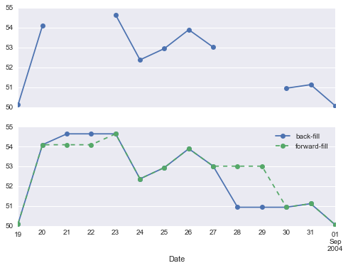
Figure 3-7. Comparison between forward-fill and back-fill interpolation
The top panel is the default: non-business days are left as NA values and do not appear on the plot. The bottom panel shows the differences between two strategies for filling the gaps: forward-filling and backward-filling.
Time-shifts
Another common time series–specific operation is shifting of data in
time. Pandas has two closely related methods for computing this:
shift() and tshift(). In short, the difference between them is that
shift() shifts the data, while tshift() shifts the index. In
both cases, the shift is specified in multiples of the frequency.
Here we will both shift() and tshift() by 900 days (Figure 3-8):
In[31]:fig,ax=plt.subplots(3,sharey=True)# apply a frequency to the datagoog=goog.asfreq('D',method='pad')goog.plot(ax=ax[0])goog.shift(900).plot(ax=ax[1])goog.tshift(900).plot(ax=ax[2])# legends and annotationslocal_max=pd.to_datetime('2007-11-05')offset=pd.Timedelta(900,'D')ax[0].legend(['input'],loc=2)ax[0].get_xticklabels()[4].set(weight='heavy',color='red')ax[0].axvline(local_max,alpha=0.3,color='red')ax[1].legend(['shift(900)'],loc=2)ax[1].get_xticklabels()[4].set(weight='heavy',color='red')ax[1].axvline(local_max+offset,alpha=0.3,color='red')ax[2].legend(['tshift(900)'],loc=2)ax[2].get_xticklabels()[1].set(weight='heavy',color='red')ax[2].axvline(local_max+offset,alpha=0.3,color='red');
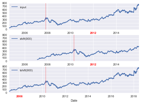
Figure 3-8. Comparison between shift and tshift
We see here that shift(900) shifts the data by 900 days, pushing
some of it off the end of the graph (and leaving NA values at the other
end), while tshift(900) shifts the index values by 900 days.
A common context for this type of shift is computing differences over time. For example, we use shifted values to compute the one-year return on investment for Google stock over the course of the dataset (Figure 3-9):
In[32]:ROI=100*(goog.tshift(-365)/goog-1)ROI.plot()plt.ylabel('% Return on Investment');
Figure 3-9. Return on investment to present day for Google stock
This helps us to see the overall trend in Google stock: thus far, the most profitable times to invest in Google have been (unsurprisingly, in retrospect) shortly after its IPO, and in the middle of the 2009 recession.
Rolling windows
Rolling statistics are a third type of time series–specific operation
implemented by Pandas. These can be accomplished via the rolling()
attribute of Series and DataFrame objects, which returns a view similar
to what we saw with the groupby operation (see
“Aggregation and Grouping”).
This rolling view makes available a number of aggregation operations by
default.
For example, here is the one-year centered rolling mean and standard deviation of the Google stock prices (Figure 3-10):
In[33]:rolling=goog.rolling(365,center=True)data=pd.DataFrame({'input':goog,'one-year rolling_mean':rolling.mean(),'one-year rolling_std':rolling.std()})ax=data.plot(style=['-','--',':'])ax.lines[0].set_alpha(0.3)
Figure 3-10. Rolling statistics on Google stock prices
As with groupby operations, the aggregate() and apply() methods can
be used for custom rolling computations.
Where to Learn More
This section has provided only a brief summary of some of the most essential features of time series tools provided by Pandas; for a more complete discussion, you can refer to the “Time Series/Date” section of the Pandas online documentation.
Another excellent resource is the textbook Python for Data Analysis by Wes McKinney (O’Reilly, 2012). Although it is now a few years old, it is an invaluable resource on the use of Pandas. In particular, this book emphasizes time series tools in the context of business and finance, and focuses much more on particular details of business calendars, time zones, and related topics.
As always, you can also use the IPython help functionality to explore and try further options available to the functions and methods discussed here. I find this often is the best way to learn a new Python tool.
Example: Visualizing Seattle Bicycle Counts
As a more involved example of working with some time series data, let’s take a look at bicycle counts on Seattle’s Fremont Bridge. This data comes from an automated bicycle counter, installed in late 2012, which has inductive sensors on the east and west sidewalks of the bridge. The hourly bicycle counts can be downloaded from http://data.seattle.gov/; here is the direct link to the dataset.
As of summer 2016, the CSV can be downloaded as follows:
In[34]:# !curl -o FremontBridge.csv# https://data.seattle.gov/api/views/65db-xm6k/rows.csv?accessType=DOWNLOAD
Once this dataset is downloaded, we can use Pandas to read the CSV
output into a DataFrame. We will specify that we want the Date as an
index, and we want these dates to be automatically parsed:
In[35]:data=pd.read_csv('FremontBridge.csv',index_col='Date',parse_dates=True)data.head()
Out[35]: Fremont Bridge West Sidewalk \\
Date
2012-10-03 00:00:00 4.0
2012-10-03 01:00:00 4.0
2012-10-03 02:00:00 1.0
2012-10-03 03:00:00 2.0
2012-10-03 04:00:00 6.0
Fremont Bridge East Sidewalk
Date
2012-10-03 00:00:00 9.0
2012-10-03 01:00:00 6.0
2012-10-03 02:00:00 1.0
2012-10-03 03:00:00 3.0
2012-10-03 04:00:00 1.0
For convenience, we’ll further process this dataset by shortening the column names and adding a “Total” column:
In[36]:data.columns=['West','East']data['Total']=data.eval('West + East')
Now let’s take a look at the summary statistics for this data:
In[37]:data.dropna().describe()
Out[37]: West East Total
count 33544.000000 33544.000000 33544.000000
mean 61.726568 53.541706 115.268275
std 83.210813 76.380678 144.773983
min 0.000000 0.000000 0.000000
25% 8.000000 7.000000 16.000000
50% 33.000000 28.000000 64.000000
75% 80.000000 66.000000 151.000000
max 825.000000 717.000000 1186.000000
Visualizing the data
We can gain some insight into the dataset by visualizing it. Let’s start by plotting the raw data (Figure 3-11):
In[38]:%matplotlibinlineimportseaborn;seaborn.set()
In[39]:data.plot()plt.ylabel('Hourly Bicycle Count');
Figure 3-11. Hourly bicycle counts on Seattle’s Fremont bridge
The ~25,000 hourly samples are far too dense for us to make much sense of. We can gain more insight by resampling the data to a coarser grid. Let’s resample by week (Figure 3-12):
In[40]:weekly=data.resample('W').sum()weekly.plot(style=[':','--','-'])plt.ylabel('Weekly bicycle count');
This shows us some interesting seasonal trends: as you might expect, people bicycle more in the summer than in the winter, and even within a particular season the bicycle use varies from week to week (likely dependent on weather; see “In Depth: Linear Regression” where we explore this further).
Figure 3-12. Weekly bicycle crossings of Seattle’s Fremont bridge
Another way that comes in handy for aggregating the data is to use a rolling mean, utilizing the pd.rolling_mean() function. Here we’ll do a 30-day rolling mean of
our data, making sure to center the window (Figure 3-13):
In[41]:daily=data.resample('D').sum()daily.rolling(30,center=True).sum().plot(style=[':','--','-'])plt.ylabel('mean hourly count');
Figure 3-13. Rolling mean of weekly bicycle counts
The jaggedness of the result is due to the hard cutoff of the window. We can get a smoother version of a rolling mean using a window function—for example, a Gaussian window. The following code (visualized in Figure 3-14) specifies both the width of the window (we chose 50 days) and the width of the Gaussian within the window (we chose 10 days):
In[42]:daily.rolling(50,center=True,win_type='gaussian').sum(std=10).plot(style=[':','--','-']);
Figure 3-14. Gaussian smoothed weekly bicycle counts
Digging into the data
While the smoothed data views in Figure 3-14 are useful to get an idea of the general
trend in the data, they hide much of the interesting structure. For
example, we might want to look at the average traffic as a function of
the time of day. We can do this using the GroupBy functionality
discussed in “Aggregation and Grouping” (Figure 3-15):
In[43]:by_time=data.groupby(data.index.time).mean()hourly_ticks=4*60*60*np.arange(6)by_time.plot(xticks=hourly_ticks,style=[':','--','-']);
The hourly traffic is a strongly bimodal distribution, with peaks around 8:00 in the morning and 5:00 in the evening. This is likely evidence of a strong component of commuter traffic crossing the bridge. This is further evidenced by the differences between the western sidewalk (generally used going toward downtown Seattle), which peaks more strongly in the morning, and the eastern sidewalk (generally used going away from downtown Seattle), which peaks more strongly in the evening.
Figure 3-15. Average hourly bicycle counts
We also might be curious about how things change based on the day of the
week. Again, we can do this with a simple groupby (Figure 3-16):
In[44]:by_weekday=data.groupby(data.index.dayofweek).mean()by_weekday.index=['Mon','Tues','Wed','Thurs','Fri','Sat','Sun']by_weekday.plot(style=[':','--','-']);
Figure 3-16. Average daily bicycle counts
This shows a strong distinction between weekday and weekend totals, with around twice as many average riders crossing the bridge on Monday through Friday than on Saturday and Sunday.
With this in mind, let’s do a compound groupby and look at the hourly
trend on weekdays versus weekends. We’ll start by grouping by both a flag
marking the weekend, and the time of day:
In[45]:weekend=np.where(data.index.weekday<5,'Weekday','Weekend')by_time=data.groupby([weekend,data.index.time]).mean()
Now we’ll use some of the Matplotlib tools described in “Multiple Subplots” to plot two panels side by side (Figure 3-17):
In[46]:importmatplotlib.pyplotaspltfig,ax=plt.subplots(1,2,figsize=(14,5))by_time.ix['Weekday'].plot(ax=ax[0],title='Weekdays',xticks=hourly_ticks,style=[':','--','-'])by_time.ix['Weekend'].plot(ax=ax[1],title='Weekends',xticks=hourly_ticks,style=[':','--','-']);
Figure 3-17. Average hourly bicycle counts by weekday and weekend
The result is very interesting: we see a bimodal commute pattern during the work week, and a unimodal recreational pattern during the weekends. It would be interesting to dig through this data in more detail, and examine the effect of weather, temperature, time of year, and other factors on people’s commuting patterns; for further discussion, see my blog post “Is Seattle Really Seeing an Uptick In Cycling?”, which uses a subset of this data. We will also revisit this dataset in the context of modeling in “In Depth: Linear Regression”.
High-Performance Pandas: eval() and query()
As we’ve already seen in previous chapters, the power of the PyData stack is built upon the ability of NumPy and Pandas to push basic operations into C via an intuitive syntax: examples are vectorized/broadcasted operations in NumPy, and grouping-type operations in Pandas. While these abstractions are efficient and effective for many common use cases, they often rely on the creation of temporary intermediate objects, which can cause undue overhead in computational time and memory use.
As of version 0.13 (released January 2014), Pandas includes some
experimental tools that allow you to directly access C-speed operations
without costly allocation of intermediate arrays. These are the eval()
and query() functions, which rely on the
Numexpr package. In this notebook we
will walk through their use and give some rules of thumb about when you
might think about using them.
Motivating query() and eval(): Compound Expressions
We’ve seen previously that NumPy and Pandas support fast vectorized operations; for example, when you are adding the elements of two arrays:
In[1]:importnumpyasnprng=np.random.RandomState(42)x=rng.rand(1E6)y=rng.rand(1E6)%timeitx+y
100 loops, best of 3: 3.39 ms per loop
As discussed in “Computation on NumPy Arrays: Universal Functions”, this is much faster than doing the addition via a Python loop or comprehension:
In[2]:%timeitnp.fromiter((xi+yiforxi,yiinzip(x,y)),dtype=x.dtype,count=len(x))
1 loop, best of 3: 266 ms per loop
But this abstraction can become less efficient when you are computing compound expressions. For example, consider the following expression:
In[3]:mask=(x>0.5)&(y<0.5)
Because NumPy evaluates each subexpression, this is roughly equivalent to the following:
In[4]:tmp1=(x>0.5)tmp2=(y<0.5)mask=tmp1&tmp2
In other words, every intermediate step is explicitly allocated in
memory. If the x and y arrays are very large, this can lead to
significant memory and computational overhead. The Numexpr library gives
you the ability to compute this type of compound expression
element by element, without the need to allocate full intermediate
arrays. The Numexpr documentation has
more details, but for the time being it is sufficient to say that the
library accepts a string giving the NumPy-style expression you’d like
to compute:
In[5]:importnumexprmask_numexpr=numexpr.evaluate('(x > 0.5) & (y < 0.5)')np.allclose(mask,mask_numexpr)
Out[5]: True
The benefit here is that Numexpr evaluates the expression in a way that
does not use full-sized temporary arrays, and thus can be much more
efficient than NumPy, especially for large arrays. The Pandas eval()
and query() tools that we will discuss here are conceptually similar, and depend
on the Numexpr package.
pandas.eval() for Efficient Operations
The eval() function in Pandas uses string expressions to efficiently
compute operations using DataFrames. For example, consider the following
DataFrames:
In[6]:importpandasaspdnrows,ncols=100000,100rng=np.random.RandomState(42)df1,df2,df3,df4=(pd.DataFrame(rng.rand(nrows,ncols))foriinrange(4))
To compute the sum of all four DataFrames using the typical Pandas
approach, we can just write the sum:
In[7]:%timeitdf1+df2+df3+df4
10 loops, best of 3: 87.1 ms per loop
We can compute the same result via pd.eval by constructing the
expression as a string:
In[8]:%timeitpd.eval('df1 + df2 + df3 + df4')
10 loops, best of 3: 42.2 ms per loop
The eval() version of this expression is about 50% faster (and uses
much less memory), while giving the same result:
In[9]:np.allclose(df1+df2+df3+df4,pd.eval('df1 + df2 + df3 + df4'))
Out[9]: True
Operations supported by pd.eval()
As of Pandas v0.16, pd.eval() supports a wide range of operations. To
demonstrate these, we’ll use the following integer DataFrames:
In[10]:df1,df2,df3,df4,df5=(pd.DataFrame(rng.randint(0,1000,(100,3)))foriinrange(5))
Arithmetic operators
pd.eval() supports all arithmetic operators. For example:
In[11]:result1=-df1*df2/(df3+df4)-df5result2=pd.eval('-df1 * df2 / (df3 + df4) - df5')np.allclose(result1,result2)
Out[11]: True
Comparison operators
pd.eval() supports all comparison operators, including chained
expressions:
In[12]:result1=(df1<df2)&(df2<=df3)&(df3!=df4)result2=pd.eval('df1 < df2 <= df3 != df4')np.allclose(result1,result2)
Out[12]: True
Bitwise operators
pd.eval() supports the & and | bitwise operators:
In[13]:result1=(df1<0.5)&(df2<0.5)|(df3<df4)result2=pd.eval('(df1 < 0.5) & (df2 < 0.5) | (df3 < df4)')np.allclose(result1,result2)
Out[13]: True
In addition, it supports the use of the literal and and or in
Boolean expressions:
In[14]:result3=pd.eval('(df1 < 0.5) and (df2 < 0.5) or (df3 < df4)')np.allclose(result1,result3)
Out[14]: True
Object attributes and indices
pd.eval() supports access to object attributes via the obj.attr
syntax, and indexes via the obj[index] syntax:
In[15]:result1=df2.T[0]+df3.iloc[1]result2=pd.eval('df2.T[0] + df3.iloc[1]')np.allclose(result1,result2)
Out[15]: True
DataFrame.eval() for Column-Wise Operations
Just as Pandas has a top-level pd.eval() function, DataFrames have an
eval() method that works in similar ways. The benefit of the eval()
method is that columns can be referred to by name. We’ll use this
labeled array as an example:
In[16]:df=pd.DataFrame(rng.rand(1000,3),columns=['A','B','C'])df.head()
Out[16]: A B C
0 0.375506 0.406939 0.069938
1 0.069087 0.235615 0.154374
2 0.677945 0.433839 0.652324
3 0.264038 0.808055 0.347197
4 0.589161 0.252418 0.557789
Using pd.eval() as above, we can compute expressions with the three
columns like this:
In[17]:result1=(df['A']+df['B'])/(df['C']-1)result2=pd.eval("(df.A + df.B) / (df.C - 1)")np.allclose(result1,result2)
Out[17]: True
The DataFrame.eval() method allows much more succinct evaluation of
expressions with the columns:
In[18]:result3=df.eval('(A + B) / (C - 1)')np.allclose(result1,result3)
Out[18]: True
Notice here that we treat column names as variables within the evaluated expression, and the result is what we would wish.
Assignment in DataFrame.eval()
In addition to the options just discussed, DataFrame.eval() also
allows assignment to any column. Let’s use the DataFrame from before,
which has columns 'A', 'B', and 'C':
In[19]:df.head()
Out[19]: A B C
0 0.375506 0.406939 0.069938
1 0.069087 0.235615 0.154374
2 0.677945 0.433839 0.652324
3 0.264038 0.808055 0.347197
4 0.589161 0.252418 0.557789
We can use df.eval() to create a new column 'D' and assign to it a
value computed from the other columns:
In[20]:df.eval('D = (A + B) / C',inplace=True)df.head()
Out[20]: A B C D
0 0.375506 0.406939 0.069938 11.187620
1 0.069087 0.235615 0.154374 1.973796
2 0.677945 0.433839 0.652324 1.704344
3 0.264038 0.808055 0.347197 3.087857
4 0.589161 0.252418 0.557789 1.508776
In the same way, any existing column can be modified:
In[21]:df.eval('D = (A - B) / C',inplace=True)df.head()
Out[21]: A B C D
0 0.375506 0.406939 0.069938 -0.449425
1 0.069087 0.235615 0.154374 -1.078728
2 0.677945 0.433839 0.652324 0.374209
3 0.264038 0.808055 0.347197 -1.566886
4 0.589161 0.252418 0.557789 0.603708
Local variables in DataFrame.eval()
The DataFrame.eval() method supports an additional syntax that lets
it work with local Python variables. Consider the following:
In[22]:column_mean=df.mean(1)result1=df['A']+column_meanresult2=df.eval('A + @column_mean')np.allclose(result1,result2)
Out[22]: True
The @ character here marks a variable name rather than a column
name, and lets you efficiently evaluate expressions involving the two
“namespaces”: the namespace of columns, and the namespace of Python
objects. Notice that this @ character is only supported by the
DataFrame.eval() method, not by the pandas.eval() function,
because the pandas.eval() function only has access to the one (Python)
namespace.
DataFrame.query() Method
The DataFrame has another method based on evaluated strings, called the
query() method. Consider the following:
In[23]:result1=df[(df.A<0.5)&(df.B<0.5)]result2=pd.eval('df[(df.A < 0.5) & (df.B < 0.5)]')np.allclose(result1,result2)
Out[23]: True
As with the example used in our discussion of DataFrame.eval(), this is an expression
involving columns of the DataFrame. It cannot be expressed
using the DataFrame.eval() syntax, however! Instead, for this type of filtering
operation, you can use the query() method:
In[24]:result2=df.query('A < 0.5 and B < 0.5')np.allclose(result1,result2)
Out[24]: True
In addition to being a more efficient computation, compared to the
masking expression this is much easier to read and understand. Note that
the query() method also accepts the @ flag to mark local variables:
In[25]:Cmean=df['C'].mean()result1=df[(df.A<Cmean)&(df.B<Cmean)]result2=df.query('A < @Cmean and B < @Cmean')np.allclose(result1,result2)
Out[25]: True
Performance: When to Use These Functions
When considering whether to use these functions, there are two
considerations: computation time and memory use. Memory use is the
most predictable aspect. As already mentioned, every compound expression
involving NumPy arrays or Pandas DataFrames will result in implicit
creation of temporary arrays: For example, this:
In[26]:x=df[(df.A<0.5)&(df.B<0.5)]
is roughly equivalent to this:
In[27]:tmp1=df.A<0.5tmp2=df.B<0.5tmp3=tmp1&tmp2x=df[tmp3]
If the size of the temporary DataFrames is significant compared to your
available system memory (typically several gigabytes), then it’s a good
idea to use an eval() or query() expression. You can check the
approximate size of your array in bytes using this:
In[28]:df.values.nbytes
Out[28]: 32000
On the performance side, eval() can be faster even when you are not
maxing out your system memory. The issue is how your temporary
DataFrames compare to the size of the L1 or L2 CPU cache on your system
(typically a few megabytes in 2016); if they are much bigger, then
eval() can avoid some potentially slow movement of values between the
different memory caches. In practice, I find that the difference in
computation time between the traditional methods and the eval/query
method is usually not significant—if anything, the traditional method
is faster for smaller arrays! The benefit of eval/query is mainly in
the saved memory, and the sometimes cleaner syntax they offer.
We’ve covered most of the details of eval() and query() here; for
more information on these, you can refer to the Pandas documentation. In
particular, different parsers and engines can be specified for running
these queries; for details on this, see the discussion within the
“Enhancing
Performance” section.
Further Resources
In this chapter, we’ve covered many of the basics of using Pandas effectively for data analysis. Still, much has been omitted from our discussion. To learn more about Pandas, I recommend the following resources:
- Pandas online documentation
-
This is the go-to source for complete documentation of the package. While the examples in the documentation tend to be small generated datasets, the description of the options is complete and generally very useful for understanding the use of various functions.
- Python for Data Analysis
-
Written by Wes McKinney (the original creator of Pandas), this book contains much more detail on the package than we had room for in this chapter. In particular, he takes a deep dive into tools for time series, which were his bread and butter as a financial consultant. The book also has many entertaining examples of applying Pandas to gain insight from real-world datasets. Keep in mind, though, that the book is now several years old, and the Pandas package has quite a few new features that this book does not cover (but be on the lookout for a new edition in 2017).
- Pandas on Stack Overflow
-
Pandas has so many users that any question you have has likely been asked and answered on Stack Overflow. Using Pandas is a case where some Google-Fu is your best friend. Simply go to your favorite search engine and type in the question, problem, or error you’re coming across—more than likely you’ll find your answer on a Stack Overflow page.
- Pandas on PyVideo
-
From PyCon to SciPy to PyData, many conferences have featured tutorials from Pandas developers and power users. The PyCon tutorials in particular tend to be given by very well-vetted presenters.
My hope is that, by using these resources, combined with the walk-through given in this chapter, you’ll be poised to use Pandas to tackle any data analysis problem you come across!
1 You can learn more about sigma-clipping operations in a book I coauthored with Željko Ivezić, Andrew J. Connolly, and Alexander Gray: Statistics, Data Mining, and Machine Learning in Astronomy: A Practical Python Guide for the Analysis of Survey Data (Princeton University Press, 2014).