Essential Tools for Working with Data
Copyright © 2017 Jake VanderPlas. All rights reserved.
Printed in the United States of America.
Published by O’Reilly Media, Inc., 1005 Gravenstein Highway North, Sebastopol, CA 95472.
O’Reilly books may be purchased for educational, business, or sales promotional use. Online editions are also available for most titles (http://oreilly.com/safari). For more information, contact our corporate/institutional sales department: 800-998-9938 or corporate@oreilly.com.
See http://oreilly.com/catalog/errata.csp?isbn=9781491912058 for release details.
The O’Reilly logo is a registered trademark of O’Reilly Media, Inc. Python Data Science Handbook, the cover image, and related trade dress are trademarks of O’Reilly Media, Inc.
While the publisher and the author have used good faith efforts to ensure that the information and instructions contained in this work are accurate, the publisher and the author disclaim all responsibility for errors or omissions, including without limitation responsibility for damages resulting from the use of or reliance on this work. Use of the information and instructions contained in this work is at your own risk. If any code samples or other technology this work contains or describes is subject to open source licenses or the intellectual property rights of others, it is your responsibility to ensure that your use thereof complies with such licenses and/or rights.
978-1-491-91205-8
[LSI]
This is a book about doing data science with Python, which immediately begs the question: what is data science? It’s a surprisingly hard definition to nail down, especially given how ubiquitous the term has become. Vocal critics have variously dismissed the term as a superfluous label (after all, what science doesn’t involve data?) or a simple buzzword that only exists to salt résumés and catch the eye of overzealous tech recruiters.
In my mind, these critiques miss something important. Data science, despite its hype-laden veneer, is perhaps the best label we have for the cross-disciplinary set of skills that are becoming increasingly important in many applications across industry and academia. This cross-disciplinary piece is key: in my mind, the best existing definition of data science is illustrated by Drew Conway’s Data Science Venn Diagram, first published on his blog in September 2010 (see Figure P-1).
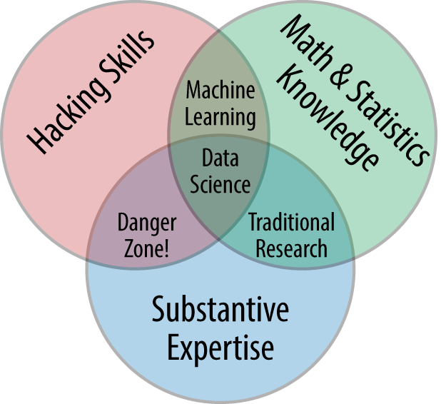
While some of the intersection labels are a bit tongue-in-cheek, this diagram captures the essence of what I think people mean when they say “data science”: it is fundamentally an interdisciplinary subject. Data science comprises three distinct and overlapping areas: the skills of a statistician who knows how to model and summarize datasets (which are growing ever larger); the skills of a computer scientist who can design and use algorithms to efficiently store, process, and visualize this data; and the domain expertise—what we might think of as “classical” training in a subject—necessary both to formulate the right questions and to put their answers in context.
With this in mind, I would encourage you to think of data science not as a new domain of knowledge to learn, but as a new set of skills that you can apply within your current area of expertise. Whether you are reporting election results, forecasting stock returns, optimizing online ad clicks, identifying microorganisms in microscope photos, seeking new classes of astronomical objects, or working with data in any other field, the goal of this book is to give you the ability to ask and answer new questions about your chosen subject area.
In my teaching both at the University of Washington and at various tech-focused conferences and meetups, one of the most common questions I have heard is this: “how should I learn Python?” The people asking are generally technically minded students, developers, or researchers, often with an already strong background in writing code and using computational and numerical tools. Most of these folks don’t want to learn Python per se, but want to learn the language with the aim of using it as a tool for data-intensive and computational science. While a large patchwork of videos, blog posts, and tutorials for this audience is available online, I’ve long been frustrated by the lack of a single good answer to this question; that is what inspired this book.
The book is not meant to be an introduction to Python or to programming in general; I assume the reader has familiarity with the Python language, including defining functions, assigning variables, calling methods of objects, controlling the flow of a program, and other basic tasks. Instead, it is meant to help Python users learn to use Python’s data science stack—libraries such as IPython, NumPy, Pandas, Matplotlib, Scikit-Learn, and related tools—to effectively store, manipulate, and gain insight from data.
Python has emerged over the last couple decades as a first-class tool for scientific computing tasks, including the analysis and visualization of large datasets. This may have come as a surprise to early proponents of the Python language: the language itself was not specifically designed with data analysis or scientific computing in mind. The usefulness of Python for data science stems primarily from the large and active ecosystem of third-party packages: NumPy for manipulation of homogeneous array-based data, Pandas for manipulation of heterogeneous and labeled data, SciPy for common scientific computing tasks, Matplotlib for publication-quality visualizations, IPython for interactive execution and sharing of code, Scikit-Learn for machine learning, and many more tools that will be mentioned in the following pages.
If you are looking for a guide to the Python language itself, I would suggest the sister project to this book, A Whirlwind Tour of the Python Language. This short report provides a tour of the essential features of the Python language, aimed at data scientists who already are familiar with one or more other programming languages.
This book uses the syntax of Python 3, which contains language enhancements that are not compatible with the 2.x series of Python. Though Python 3.0 was first released in 2008, adoption has been relatively slow, particularly in the scientific and web development communities. This is primarily because it took some time for many of the essential third-party packages and toolkits to be made compatible with the new language internals. Since early 2014, however, stable releases of the most important tools in the data science ecosystem have been fully compatible with both Python 2 and 3, and so this book will use the newer Python 3 syntax. However, the vast majority of code snippets in this book will also work without modification in Python 2: in cases where a Py2-incompatible syntax is used, I will make every effort to note it explicitly.
Each chapter of this book focuses on a particular package or tool that contributes a fundamental piece of the Python data science story.
These packages provide the computational environment in which many Python-using data scientists work.
This library provides the ndarray object for efficient storage and manipulation of dense data arrays in Python.
This library provides the DataFrame object for efficient storage
and manipulation of labeled/columnar data in Python.
This library provides capabilities for a flexible range of data visualizations in Python.
This library provides efficient and clean Python implementations of the most important and established machine learning algorithms.
The PyData world is certainly much larger than these five packages, and is growing every day. With this in mind, I make every attempt through these pages to provide references to other interesting efforts, projects, and packages that are pushing the boundaries of what can be done in Python. Nevertheless, these five are currently fundamental to much of the work being done in the Python data science space, and I expect they will remain important even as the ecosystem continues growing around them.
Supplemental material (code examples, figures, etc.) is available for download at https://github.com/jakevdp/PythonDataScienceHandbook. This book is here to help you get your job done. In general, if example code is offered with this book, you may use it in your programs and documentation. You do not need to contact us for permission unless you’re reproducing a significant portion of the code. For example, writing a program that uses several chunks of code from this book does not require permission. Selling or distributing a CD-ROM of examples from O’Reilly books does require permission. Answering a question by citing this book and quoting example code does not require permission. Incorporating a significant amount of example code from this book into your product’s documentation does require permission.
We appreciate, but do not require, attribution. An attribution usually includes the title, author, publisher, and ISBN. For example, “Python Data Science Handbook by Jake VanderPlas (O’Reilly). Copyright 2017 Jake VanderPlas, 978-1-491-91205-8.”
If you feel your use of code examples falls outside fair use or the permission given above, feel free to contact us at permissions@oreilly.com.
Installing Python and the suite of libraries that enable scientific computing is straightforward. This section will outline some of the considerations to keep in mind when setting up your computer.
Though there are various ways to install Python, the one I would suggest for use in data science is the Anaconda distribution, which works similarly whether you use Windows, Linux, or Mac OS X. The Anaconda distribution comes in two flavors:
Miniconda gives you the Python interpreter itself, along with a command-line tool called conda that operates as a cross-platform package manager geared toward Python packages, similar in spirit to the apt or yum tools that Linux users might be familiar with.
Anaconda includes both Python and conda, and additionally bundles a suite of other preinstalled packages geared toward scientific computing. Because of the size of this bundle, expect the installation to consume several gigabytes of disk space.
Any of the packages included with Anaconda can also be installed manually on top of Miniconda; for this reason I suggest starting with Miniconda.
To get started, download and install the Miniconda package (make sure to choose a version with Python 3), and then install the core packages used in this book:
[~]$ conda install numpy pandas scikit-learn matplotlib seaborn ipython-notebook
Throughout the text, we will also make use of other, more specialized tools
in Python’s scientific ecosystem; installation is usually as easy as
typing conda install packagename. For more information on conda,
including information about creating and using conda environments (which
I would highly recommend), refer to
conda’s online documentation.
The following typographical conventions are used in this book:
Indicates new terms, URLs, email addresses, filenames, and file extensions.
Constant widthUsed for program listings, as well as within paragraphs to refer to program elements such as variable or function names, databases, data types, environment variables, statements, and keywords.
Constant width boldShows commands or other text that should be typed literally by the user.
Constant width italicShows text that should be replaced with user-supplied values or by values determined by context.
Safari (formerly Safari Books Online) is a membership-based training and reference platform for enterprise, government, educators, and individuals.
Members have access to thousands of books, training videos, Learning Paths, interactive tutorials, and curated playlists from over 250 publishers, including O’Reilly Media, Harvard Business Review, Prentice Hall Professional, Addison-Wesley Professional, Microsoft Press, Sams, Que, Peachpit Press, Adobe, Focal Press, Cisco Press, John Wiley & Sons, Syngress, Morgan Kaufmann, IBM Redbooks, Packt, Adobe Press, FT Press, Apress, Manning, New Riders, McGraw-Hill, Jones & Bartlett, and Course Technology, among others.
For more information, please visit http://oreilly.com/safari.
Please address comments and questions concerning this book to the publisher:
We have a web page for this book, where we list errata, examples, and any additional information. You can access this page at http://bit.ly/python-data-sci-handbook.
To comment or ask technical questions about this book, send email to bookquestions@oreilly.com.
For more information about our books, courses, conferences, and news, see our website at http://www.oreilly.com.
Find us on Facebook: http://facebook.com/oreilly
Follow us on Twitter: http://twitter.com/oreillymedia
Watch us on YouTube: http://www.youtube.com/oreillymedia
There are many options for development environments for Python, and I’m often asked which one I use in my own work. My answer sometimes surprises people: my preferred environment is IPython plus a text editor (in my case, Emacs or Atom depending on my mood). IPython (short for Interactive Python) was started in 2001 by Fernando Perez as an enhanced Python interpreter, and has since grown into a project aiming to provide, in Perez’s words, “Tools for the entire lifecycle of research computing.” If Python is the engine of our data science task, you might think of IPython as the interactive control panel.
As well as being a useful interactive interface to Python, IPython also provides a number of useful syntactic additions to the language; we’ll cover the most useful of these additions here. In addition, IPython is closely tied with the Jupyter project, which provides a browser-based notebook that is useful for development, collaboration, sharing, and even publication of data science results. The IPython notebook is actually a special case of the broader Jupyter notebook structure, which encompasses notebooks for Julia, R, and other programming languages. As an example of the usefulness of the notebook format, look no further than the page you are reading: the entire manuscript for this book was composed as a set of IPython notebooks.
IPython is about using Python effectively for interactive scientific and data-intensive computing. This chapter will start by stepping through some of the IPython features that are useful to the practice of data science, focusing especially on the syntax it offers beyond the standard features of Python. Next, we will go into a bit more depth on some of the more useful “magic commands” that can speed up common tasks in creating and using data science code. Finally, we will touch on some of the features of the notebook that make it useful in understanding data and sharing results.
There are two primary means of using IPython that we’ll discuss in this chapter: the IPython shell and the IPython notebook. The bulk of the material in this chapter is relevant to both, and the examples will switch between them depending on what is most convenient. In the few sections that are relevant to just one or the other, I will explicitly state that fact. Before we start, some words on how to launch the IPython shell and IPython notebook.
This chapter, like most of this book, is not designed to be absorbed
passively. I recommend that as you read through it, you follow along and
experiment with the tools and syntax we cover: the muscle-memory you
build through doing this will be far more useful than the simple act of
reading about it. Start by launching the IPython interpreter by typing
ipython on the command line; alternatively, if you’ve installed a
distribution like Anaconda or EPD, there may be a launcher specific to
your system (we’ll discuss this more fully in “Help and Documentation in IPython”).
Once you do this, you should see a prompt like the following:
IPython 4.0.1 -- An enhanced Interactive Python. ? -> Introduction and overview of IPython's features. %quickref -> Quick reference. help -> Python's own help system. object? -> Details about 'object', use 'object??' for extra details. In [1]:
With that, you’re ready to follow along.
The Jupyter notebook is a browser-based graphical interface to the IPython shell, and builds on it a rich set of dynamic display capabilities. As well as executing Python/IPython statements, the notebook allows the user to include formatted text, static and dynamic visualizations, mathematical equations, JavaScript widgets, and much more. Furthermore, these documents can be saved in a way that lets other people open them and execute the code on their own systems.
Though the IPython notebook is viewed and edited through your web browser window, it must connect to a running Python process in order to execute code. To start this process (known as a “kernel”), run the following command in your system shell:
$ jupyter notebook
This command will launch a local web server that will be visible to your browser. It immediately spits out a log showing what it is doing; that log will look something like this:
$ jupyter notebook [NotebookApp] Serving notebooks from local directory: /Users/jakevdp/... [NotebookApp] 0 active kernels [NotebookApp] The IPython Notebook is running at: http://localhost:8888/ [NotebookApp] Use Control-C to stop this server and shut down all kernels...
Upon issuing the command, your default browser should automatically open and navigate to the listed local URL; the exact address will depend on your system. If the browser does not open automatically, you can open a window and manually open this address (http://localhost:8888/ in this example).
If you read no other section in this chapter, read this one: I find the tools discussed here to be the most transformative contributions of IPython to my daily workflow.
When a technologically minded person is asked to help a friend, family member, or colleague with a computer problem, most of the time it’s less a matter of knowing the answer as much as knowing how to quickly find an unknown answer. In data science it’s the same: searchable web resources such as online documentation, mailing-list threads, and Stack Overflow answers contain a wealth of information, even (especially?) if it is a topic you’ve found yourself searching before. Being an effective practitioner of data science is less about memorizing the tool or command you should use for every possible situation, and more about learning to effectively find the information you don’t know, whether through a web search engine or another means.
One of the most useful functions of IPython/Jupyter is to shorten the gap between the user and the type of documentation and search that will help them do their work effectively. While web searches still play a role in answering complicated questions, an amazing amount of information can be found through IPython alone. Some examples of the questions IPython can help answer in a few keystrokes:
How do I call this function? What arguments and options does it have?
What does the source code of this Python object look like?
What is in this package I imported? What attributes or methods does this object have?
Here we’ll discuss IPython’s tools to quickly access this information,
namely the ? character to explore documentation, the ?? characters
to explore source code, and the Tab key for autocompletion.
The Python language and its data science ecosystem are built with the
user in mind, and one big part of that is access to documentation. Every
Python object contains the reference to a string, known as a docstring, which in most cases will contain a concise summary of the
object and how to use it. Python has a built-in help() function that can access this information and print the results. For example, to see
the documentation of the built-in len function, you can do the
following:
In[1]:help(len)Helponbuilt-infunctionleninmodulebuiltins:len(...)len(object)->integerReturnthenumberofitemsofasequenceormapping.
Depending on your interpreter, this information may be displayed as inline text, or in some separate pop-up window.
Because finding help on an object is so common and useful, IPython
introduces the ? character as a shorthand for accessing this
documentation and other relevant information:
In[2]:len?Type:builtin_function_or_methodStringform:<built-infunctionlen>Namespace:PythonbuiltinDocstring:len(object)->integerReturnthenumberofitemsofasequenceormapping.
This notation works for just about anything, including object methods:
In[3]:L=[1,2,3]In[4]:L.insert?Type:builtin_function_or_methodStringform:<built-inmethodinsertoflistobjectat0x1024b8ea8>Docstring:L.insert(index,object)--insertobjectbeforeindex
or even objects themselves, with the documentation from their type:
In[5]:L?Type:listStringform:[1,2,3]Length:3Docstring:list()->newemptylistlist(iterable)->newlistinitializedfromiterable's items
Importantly, this will even work for functions or other objects you create yourself! Here we’ll define a small function with a docstring:
In[6]:defsquare(a):....:"""Return the square of a."""....:returna**2....:
Note that to create a docstring for our function, we simply placed a string literal in the first line. Because docstrings are usually multiple lines, by convention we used Python’s triple-quote notation for multiline strings.
Now we’ll use the ? mark to find this docstring:
In[7]:square?Type:functionStringform:<functionsquareat0x103713cb0>Definition:square(a)Docstring:Returnthesquareofa.
This quick access to documentation via docstrings is one reason you should get in the habit of always adding such inline documentation to the code you write!
Because the Python language is so easily readable, you can usually gain another level of
insight by reading the source code of the object
you’re curious about. IPython provides a shortcut to the source code
with the double question mark (??):
In[8]:square??Type:functionStringform:<functionsquareat0x103713cb0>Definition:square(a)Source:defsquare(a):"Return the square of a"returna**2
For simple functions like this, the double question mark can give quick insight into the under-the-hood details.
If you play with this much, you’ll notice that sometimes the ?? suffix
doesn’t display any source code: this is generally because the object in
question is not implemented in Python, but in C or some other compiled
extension language. If this is the case, the ?? suffix gives the same
output as the ? suffix. You’ll find this particularly with many of
Python’s built-in objects and types, for example len from above:
In[9]:len??Type:builtin_function_or_methodStringform:<built-infunctionlen>Namespace:PythonbuiltinDocstring:len(object)->integerReturnthenumberofitemsofasequenceormapping.
Using ? and/or ?? gives a powerful and quick interface for finding
information about what any Python function or module does.
IPython’s other useful interface is the use of the Tab key for
autocompletion and exploration of the contents of objects, modules, and
namespaces. In the examples that follow, we’ll use <TAB> to indicate when the Tab key should be pressed.
Every Python object has various attributes and methods associated with
it. Like with the help function discussed before, Python has a built-in dir
function that returns a list of these, but the tab-completion interface
is much easier to use in practice. To see a list of all available
attributes of an object, you can type the name of the object followed by
a period (.) character and the Tab key:
In[10]:L.<TAB>L.appendL.copyL.extendL.insertL.removeL.sortL.clearL.countL.indexL.popL.reverse
To narrow down the list, you can type the first character or several characters of the name, and the Tab key will find the matching attributes and methods:
In[10]:L.c<TAB>L.clearL.copyL.countIn[10]:L.co<TAB>L.copyL.count
If there is only a single option, pressing the Tab key will complete the
line for you. For example, the following will instantly be replaced with L.count:
In[10]:L.cou<TAB>
Though Python has no strictly enforced distinction between public/external attributes and private/internal attributes, by convention a preceding underscore is used to denote such methods. For clarity, these private methods and special methods are omitted from the list by default, but it’s possible to list them by explicitly typing the underscore:
In[10]:L._<TAB>L.__add__L.__gt__L.__reduce__L.__class__L.__hash__L.__reduce_ex__
For brevity, we’ve only shown the first couple lines of the output. Most of these are Python’s special double-underscore methods (often nicknamed “dunder” methods).
Tab completion is also useful when importing objects from packages. Here
we’ll use it to find all possible imports in the itertools package
that start with co:
In [10]: from itertools import co<TAB> combinations compress combinations_with_replacement count
Similarly, you can use tab completion to see which imports are available on your system (this will change depending on which third-party scripts and modules are visible to your Python session):
In [10]: import <TAB> Display all 399 possibilities? (y or n) Crypto dis py_compile Cython distutils pyclbr ... ... ... difflib pwd zmq In [10]: import h<TAB> hashlib hmac http heapq html husl
(Note that for brevity, I did not print here all 399 importable packages and modules on my system.)
Tab completion is useful if you know the first few characters of the
object or attribute you’re looking for, but is little help if you’d like
to match characters at the middle or end of the word. For this use case,
IPython provides a means of wildcard matching for names using the *
character.
For example, we can use this to list every object in the namespace that
ends with Warning:
In[10]:*Warning?BytesWarningRuntimeWarningDeprecationWarningSyntaxWarningFutureWarningUnicodeWarningImportWarningUserWarningPendingDeprecationWarningWarningResourceWarning
Notice that the * character matches any string, including the empty
string.
Similarly, suppose we are looking for a string method that contains the
word find somewhere in its name. We can search for it this way:
In[10]:str.*find*?str.findstr.rfind
I find this type of flexible wildcard search can be very useful for finding a particular command when I’m getting to know a new package or reacquainting myself with a familiar one.
If you spend any amount of time on the computer, you’ve probably found a use for keyboard shortcuts in your workflow. Most familiar perhaps are Cmd-C and Cmd-V (or Ctrl-C and Ctrl-V) for copying and pasting in a wide variety of programs and systems. Power users tend to go even further: popular text editors like Emacs, Vim, and others provide users an incredible range of operations through intricate combinations of keystrokes.
The IPython shell doesn’t go this far, but does provide a number of keyboard shortcuts for fast navigation while you’re typing commands. These shortcuts are not in fact provided by IPython itself, but through its dependency on the GNU Readline library: thus, some of the following shortcuts may differ depending on your system configuration. Also, while some of these shortcuts do work in the browser-based notebook, this section is primarily about shortcuts in the IPython shell.
Once you get accustomed to these, they can be very useful for quickly performing certain commands without moving your hands from the “home” keyboard position. If you’re an Emacs user or if you have experience with Linux-style shells, the following will be very familiar. We’ll group these shortcuts into a few categories: navigation shortcuts, text entry shortcuts, command history shortcuts, and miscellaneous shortcuts.
While everyone is familiar with using the Backspace key to delete the previous character, reaching for the key often requires some minor finger gymnastics, and it only deletes a single character at a time. In IPython there are several shortcuts for removing some portion of the text you’re typing. The most immediately useful of these are the commands to delete entire lines of text. You’ll know these have become second nature if you find yourself using a combination of Ctrl-b and Ctrl-d instead of reaching for the Backspace key to delete the previous character!
| Keystroke | Action |
|---|---|
Backspace key |
Delete previous character in line |
Ctrl-d |
Delete next character in line |
Ctrl-k |
Cut text from cursor to end of line |
Ctrl-u |
Cut text from beginning fo line to cursor |
Ctrl-y |
Yank (i.e., paste) text that was previously cut |
Ctrl-t |
Transpose (i.e., switch) previous two characters |
Perhaps the most impactful shortcuts discussed here are the ones IPython provides for navigating the command history. This command history goes beyond your current IPython session: your entire command history is stored in a SQLite database in your IPython profile directory. The most straightforward way to access these is with the up and down arrow keys to step through the history, but other options exist as well:
| Keystroke | Action |
|---|---|
Ctrl-p (or the up arrow key) |
Access previous command in history |
Ctrl-n (or the down arrow key) |
Access next command in history |
Ctrl-r |
Reverse-search through command history |
The reverse-search can be particularly useful. Recall that in the
previous section we defined a function called square. Let’s
reverse-search our Python history from a new IPython shell and find this
definition again. When you press Ctrl-r in the IPython terminal,
you’ll see the following prompt:
In[1]:(reverse-i-search)`':
If you start typing characters at this prompt, IPython will auto-fill the most recent command, if any, that matches those characters:
In[1]:(reverse-i-search)`sqa': square??
At any point, you can add more characters to refine the search, or press Ctrl-r again to search further for another command that matches the query. If you followed along in the previous section, pressing Ctrl-r twice more gives:
In[1]:(reverse-i-search)`sqa': def square(a):"""Return the square of a"""returna**2
Once you have found the command you’re looking for, press Return and the search will end. We can then use the retrieved command, and carry on with our session:
In[1]:defsquare(a):"""Return the square of a"""returna**2In[2]:square(2)Out[2]:4
Note that you can also use Ctrl-p/Ctrl-n or the up/down arrow keys to
search through history, but only by matching characters at the beginning
of the line. That is, if you type def and then press Ctrl-p, it would find the most
recent command (if any) in your history that begins with the characters
def.
Finally, there are a few miscellaneous shortcuts that don’t fit into any of the preceding categories, but are nevertheless useful to know:
| Keystroke | Action |
|---|---|
Ctrl-l |
Clear terminal screen |
Ctrl-c |
Interrupt current Python command |
Ctrl-d |
Exit IPython session |
The Ctrl-c shortcut in particular can be useful when you inadvertently start a very long-running job.
While some of the shortcuts discussed here may seem a bit tedious at first, they quickly become automatic with practice. Once you develop that muscle memory, I suspect you will even find yourself wishing they were available in other contexts.
The previous two sections showed how IPython lets you use and explore
Python efficiently and interactively. Here we’ll begin discussing some
of the enhancements that IPython adds on top of the normal Python
syntax. These are known in IPython as magic commands, and are prefixed
by the % character. These magic commands are designed to succinctly
solve various common problems in standard data analysis. Magic commands
come in two flavors: line magics, which are denoted by a single % prefix and operate on a single line of input, and cell magics, which are denoted by a
double %% prefix and operate on multiple lines of input. We’ll
demonstrate and discuss a few brief examples here, and come back to more
focused discussion of several useful magic commands later in the
chapter.
When you’re working in the IPython interpreter, one common gotcha is that pasting multiline code blocks can lead to unexpected errors, especially when indentation and interpreter markers are involved. A common case is that you find some example code on a website and want to paste it into your interpreter. Consider the following simple function:
>>>defdonothing(x):...returnx
The code is formatted as it would appear in the Python interpreter, and if you copy and paste this directly into IPython you get an error:
In[2]:>>>defdonothing(x):...:...returnx...:File"<ipython-input-20-5a66c8964687>",line2...returnx^SyntaxError:invalidsyntax
In the direct paste, the interpreter is confused by the additional
prompt characters. But never fear—IPython’s %paste magic function is
designed to handle this exact type of multiline, marked-up input:
In[3]:%paste>>>defdonothing(x):...returnx## -- End pasted text --
The %paste command both enters and executes the code, so now the
function is ready to be used:
In[4]:donothing(10)Out[4]:10
A command with a similar intent is %cpaste, which opens up an
interactive multiline prompt in which you can paste one or more chunks
of code to be executed in a batch:
In[5]:%cpastePastingcode;enter'--'aloneonthelinetostoporuseCtrl-D.:>>>defdonothing(x)::...returnx:--
These magic commands, like others we’ll see, make available functionality that would be difficult or impossible in a standard Python interpreter.
As you begin developing more extensive code, you will likely find
yourself working in both IPython for interactive exploration, as well as
a text editor to store code that you want to reuse. Rather than running
this code in a new window, it can be convenient to run it within your
IPython session. This can be done with the %run magic.
For example, imagine you’ve created a myscript.py file with the following contents:
#-------------------------------------# file: myscript.pydefsquare(x):"""square a number"""returnx**2forNinrange(1,4):(N,"squared is",square(N))
You can execute this from your IPython session as follows:
In[6]:%runmyscript.py1squaredis12squaredis43squaredis9
Note also that after you’ve run this script, any functions defined within it are available for use in your IPython session:
In[7]:square(5)Out[7]:25
There are several options to fine-tune how your code is run; you can see
the documentation in the normal way, by typing %run? in the IPython
interpreter.
Another example of a useful magic function is %timeit, which will
automatically determine the execution time of the single-line Python
statement that follows it. For example, we may want to check the
performance of a list comprehension:
In[8]:%timeitL = [n ** 2 for n in range(1000)]1000loops,bestof3:325µsperloop
The benefit of %timeit is that for short commands it will
automatically perform multiple runs in order to attain more robust
results. For multiline statements, adding a second % sign will turn
this into a cell magic that can handle multiple lines of input. For
example, here’s the equivalent construction with a for loop:
In[9]:%%timeit...: L = [] ...: for n in range(1000): ...: L.append(n ** 2) ...: 1000 loops, best of 3: 373 µs per loop
We can immediately see that list comprehensions are about 10% faster
than the equivalent for loop construction in this case. We’ll explore
%timeit and other approaches to timing and profiling code in
“Profiling and Timing Code”.
Like normal Python functions, IPython magic functions have docstrings, and this useful documentation can be accessed in the standard manner. So, for example, to read the documentation of the %timeit magic, simply type this:
In[10]:%timeit?
Documentation for other functions can be accessed similarly. To access a general description of available magic functions, including some examples, you can type this:
In[11]:%magic
For a quick and simple list of all available magic functions, type this:
In[12]:%lsmagic
Finally, I’ll mention that it is quite straightforward to define your own magic functions if you wish. We won’t discuss it here, but if you are interested, see the references listed in “More IPython Resources”.
Previously we saw that the IPython shell allows you to access previous commands with the up and down arrow keys, or equivalently the Ctrl-p/Ctrl-n shortcuts. Additionally, in both the shell and the notebook, IPython exposes several ways to obtain the output of previous commands, as well as string versions of the commands themselves. We’ll explore those here.
By now I imagine you’re quite familiar with the In[1]:/Out[1]: style
prompts used by IPython. But it turns out that these are not just pretty
decoration: they give a clue as to how you can access previous inputs
and outputs in your current session. Imagine you start a session that
looks like this:
In[1]:importmathIn[2]:math.sin(2)Out[2]:0.9092974268256817In[3]:math.cos(2)Out[3]:-0.4161468365471424
We’ve imported the built-in math package, then computed the sine and
the cosine of the number 2. These inputs and outputs are displayed in
the shell with In/Out labels, but there’s more—IPython actually
creates some Python variables called In and Out that are
automatically updated to reflect this history:
In[4]:(In)['','import math','math.sin(2)','math.cos(2)','print(In)']In[5]:OutOut[5]:{2:0.9092974268256817,3:-0.4161468365471424}
The In object is a list, which keeps track of the commands in order
(the first item in the list is a placeholder so that In[1] can refer
to the first command):
In[6]:(In[1])importmath
The Out object is not a list but a dictionary mapping input numbers to
their outputs (if any):
In[7]:(Out[2])0.9092974268256817
Note that not all operations have outputs: for example, import
statements and print statements don’t affect the output. The latter
may be surprising, but makes sense if you consider that print is a
function that returns None; for brevity, any command that returns
None is not added to Out.
Where this can be useful is if you want to interact with past results.
For example, let’s check the sum of sin(2) ** 2 and cos(2) ** 2
using the previously computed results:
In[8]:Out[2]**2+Out[3]**2Out[8]:1.0
The result is 1.0 as we’d expect from the well-known trigonometric
identity. In this case, using these previous results probably is not
necessary, but it can become very handy if you execute a very expensive
computation and want to reuse the result!
The standard Python shell contains just one simple shortcut for
accessing previous output; the variable _ (i.e., a single underscore)
is kept updated with the previous output; this works in IPython as well:
In[9]:(_)1.0
But IPython takes this a bit further—you can use a double underscore to access the second-to-last output, and a triple underscore to access the third-to-last output (skipping any commands with no output):
In[10]:(__)-0.4161468365471424In[11]:(___)0.9092974268256817
IPython stops there: more than three underscores starts to get a bit hard to count, and at that point it’s easier to refer to the output by line number.
There is one more shortcut we should mention, however—a
shorthand for Out[X] is _X (i.e., a single underscore followed by the line number):
In[12]:Out[2]Out[12]:0.9092974268256817In[13]:_2Out[13]:0.9092974268256817
Sometimes you might wish to suppress the output of a statement (this is perhaps most common with the plotting commands that we’ll explore in Chapter 4). Or maybe the command you’re executing produces a result that you’d prefer not to store in your output history, perhaps so that it can be deallocated when other references are removed. The easiest way to suppress the output of a command is to add a semicolon to the end of the line:
In[14]:math.sin(2)+math.cos(2);
Note that the result is computed silently, and the output is neither
displayed on the screen or stored in the Out dictionary:
In[15]:14inOutOut[15]:False
When working interactively with the standard Python interpreter, one of
the frustrations you’ll face is the need to switch between multiple windows to
access Python tools and system command-line tools. IPython bridges this
gap, and gives you a syntax for executing shell commands directly from
within the IPython terminal. The magic happens with the exclamation
point: anything appearing after ! on a line will be executed not by
the Python kernel, but by the system command line.
The following assumes you’re on a Unix-like system, such as Linux or Mac OS X. Some of the examples that follow will fail on Windows, which uses a different type of shell by default (though with the 2016 announcement of native Bash shells on Windows, soon this may no longer be an issue!). If you’re unfamiliar with shell commands, I’d suggest reviewing the Shell Tutorial put together by the always excellent Software Carpentry Foundation.
A full intro to using the shell/terminal/command line is well beyond the scope of this chapter, but for the uninitiated we will offer a quick introduction here. The shell is a way to interact textually with your computer. Ever since the mid-1980s, when Microsoft and Apple introduced the first versions of their now ubiquitous graphical operating systems, most computer users have interacted with their operating system through familiar clicking of menus and drag-and-drop movements. But operating systems existed long before these graphical user interfaces, and were primarily controlled through sequences of text input: at the prompt, the user would type a command, and the computer would do what the user told it to. Those early prompt systems are the precursors of the shells and terminals that most active data scientists still use today.
Someone unfamiliar with the shell might ask why you would bother with this, when you can accomplish many results by simply clicking on icons and menus. A shell user might reply with another question: why hunt icons and click menus when you can accomplish things much more easily by typing? While it might sound like a typical tech preference impasse, when moving beyond basic tasks it quickly becomes clear that the shell offers much more control of advanced tasks, though admittedly the learning curve can intimidate the average computer user.
As an example, here is a sample of a Linux/OS X shell session where a
user explores, creates, and modifies directories and files on their
system (osx:~ $ is the prompt, and everything after the $
sign is the typed command; text that is preceded by a # is meant just as description,
rather than something you would actually type in):
osx:~$echo"hello world"# echo is like Python's print functionhello world osx:~$pwd# pwd = print working directory/home/jake# this is the "path" that we're inosx:~$ls# ls = list working directory contentsnotebooks projects osx:~$cdprojects/# cd = change directoryosx:projects$pwd/home/jake/projects osx:projects$ls datasci_book mpld3 myproject.txt osx:projects$mkdir myproject# mkdir = make new directoryosx:projects$cdmyproject/ osx:myproject$mv ../myproject.txt ./# mv = move file. Here we're moving the# file myproject.txt from one directory# up (../) to the current directory (./)osx:myproject$ls myproject.txt
Notice that all of this is just a compact way to do familiar operations
(navigating a directory structure, creating a directory, moving a file,
etc.) by typing commands rather than clicking icons and menus. Note that
with just a few commands (pwd, ls, cd, mkdir, and cp) you can
do many of the most common file operations. It’s when you go beyond
these basics that the shell approach becomes really powerful.
You can use any command that works at the command line in IPython by prefixing it with the ! character. For example, the ls, pwd, and
echo commands can be run as follows:
In[1]:!lsmyproject.txtIn[2]:!pwd/home/jake/projects/myprojectIn[3]:!echo"printing from the shell"printingfromtheshell
Shell commands can not only be called from IPython, but can also be made to interact with the IPython namespace. For example, you can save the output of any shell command to a Python list using the assignment operator:
In[4]:contents=!lsIn[5]:(contents)['myproject.txt']In[6]:directory=!pwdIn[7]:(directory)['/Users/jakevdp/notebooks/tmp/myproject']
Note that these results are not returned as lists, but as a special shell return type defined in IPython:
In[8]:type(directory)IPython.utils.text.SList
This looks and acts a lot like a Python list, but has additional
functionality, such as the grep and fields methods and the s,
n, and p properties that allow you to search, filter, and display the
results in convenient ways. For more information on these, you can use
IPython’s built-in help features.
Communication in the other direction—passing Python variables into the
shell—is possible through the {varname} syntax:
In[9]:message="hello from Python"In[10]:!echo{message}hellofromPython
The curly braces contain the variable name, which is replaced by the variable’s contents in the shell command.
Code development and data analysis always require a bit of trial and error, and IPython contains tools to streamline this process. This section will briefly cover some options for controlling Python’s exception reporting, followed by exploring tools for debugging errors in code.
Most of the time when a Python script fails, it will raise an
exception. When the interpreter hits one of these exceptions,
information about the cause of the error can be found in the
traceback, which can be accessed from within Python. With the %xmode
magic function, IPython allows you to control the amount of information
printed when the exception is raised. Consider the following code:
In[1]:deffunc1(a,b):returna/bdeffunc2(x):a=xb=x-1returnfunc1(a,b)
In[2]:func2(1)
---------------------------------------------------------------------------
ZeroDivisionError Traceback (most recent call last)
<ipython-input-2-b2e110f6fc8f^gt; in <module>()
----> 1 func2(1)
<ipython-input-1-d849e34d61fb> in func2(x)
5 a = x
6 b = x - 1
----> 7 return func1(a, b)
<ipython-input-1-d849e34d61fb> in func1(a, b)
1 def func1(a, b):
----> 2 return a / b
3
4 def func2(x):
5 a = x
ZeroDivisionError: division by zero
Calling func2 results in an error, and reading the printed trace lets
us see exactly what happened. By default, this trace includes several
lines showing the context of each step that led to the error. Using the
%xmode magic function (short for exception mode), we can change what
information is printed.
%xmode takes a single argument, the mode, and there are three
possibilities: Plain, Context, and Verbose. The default is
Context, and gives output like that just shown. Plain is more compact and
gives less information:
In[3]:%xmodePlain
Exception reporting mode: Plain
In[4]:func2(1)
------------------------------------------------------------
Traceback (most recent call last):
File "<ipython-input-4-b2e110f6fc8f>", line 1, in <module>
func2(1)
File "<ipython-input-1-d849e34d61fb>", line 7, in func2
return func1(a, b)
File "<ipython-input-1-d849e34d61fb>", line 2, in func1
return a / b
ZeroDivisionError: division by zero
The Verbose mode adds some extra information, including the arguments
to any functions that are called:
In[5]:%xmodeVerbose
Exception reporting mode: Verbose
In[6]:func2(1)
---------------------------------------------------------------------------
ZeroDivisionError Traceback (most recent call last)
<ipython-input-6-b2e110f6fc8f> in <module>()
----> 1 func2(1)
global func2 = <function func2 at 0x103729320>
<ipython-input-1-d849e34d61fb> in func2(x=1)
5 a = x
6 b = x - 1
----> 7 return func1(a, b)
global func1 = <function func1 at 0x1037294d0>
a = 1
b = 0
<ipython-input-1-d849e34d61fb> in func1(a=1, b=0)
1 def func1(a, b):
----> 2 return a / b
a = 1
b = 0
3
4 def func2(x):
5 a = x
ZeroDivisionError: division by zero
This extra information can help you narrow in on why the exception is being
raised. So why not use the Verbose mode all the time? As code gets
complicated, this kind of traceback can get extremely long. Depending on
the context, sometimes the brevity of Default mode is easier to work
with.
The standard Python tool for interactive debugging is pdb, the Python
debugger. This debugger lets the user step through the code line by line
in order to see what might be causing a more difficult error. The
IPython-enhanced version of this is ipdb, the IPython debugger.
There are many ways to launch and use both these debuggers; we won’t cover them fully here. Refer to the online documentation of these two utilities to learn more.
In IPython, perhaps the most convenient interface to debugging is the
%debug magic command. If you call it after hitting an exception, it
will automatically open an interactive debugging prompt at the point of
the exception. The ipdb prompt lets you explore the current state of
the stack, explore the available variables, and even run Python
commands!
Let’s look at the most recent exception, then do some basic tasks—print
the values of a and b, and type quit to quit the debugging
session:
In[7]:%debug
> <ipython-input-1-d849e34d61fb>(2)func1()
1 def func1(a, b):
----> 2 return a / b
3
ipdb> print(a)
1
ipdb> print(b)
0
ipdb> quit
The interactive debugger allows much more than this, though—we can even step up and down through the stack and explore the values of variables there:
In[8]:%debug
> <ipython-input-1-d849e34d61fb>(2)func1()
1 def func1(a, b):
----> 2 return a / b
3
ipdb> up
> <ipython-input-1-d849e34d61fb>(7)func2()
5 a = x
6 b = x - 1
----> 7 return func1(a, b)
ipdb> print(x)
1
ipdb> up
> <ipython-input-6-b2e110f6fc8f>(1)<module>()
----> 1 func2(1)
ipdb> down
> <ipython-input-1-d849e34d61fb>(7)func2()
5 a = x
6 b = x - 1
----> 7 return func1(a, b)
ipdb> quit
This allows you to quickly find out not only what caused the error, but also what function calls led up to the error.
If you’d like the debugger to launch automatically whenever an exception
is raised, you can use the %pdb magic function to turn on this
automatic behavior:
In[9]:%xmodePlain%pdbonfunc2(1)
Exception reporting mode: Plain
Automatic pdb calling has been turned ON
Traceback (most recent call last):
File "<ipython-input-9-569a67d2d312>", line 3, in <module>
func2(1)
File "<ipython-input-1-d849e34d61fb>", line 7, in func2
return func1(a, b)
File "<ipython-input-1-d849e34d61fb>", line 2, in func1
return a / b
ZeroDivisionError: division by zero
> <ipython-input-1-d849e34d61fb>(2)func1()
1 def func1(a, b):
----> 2 return a / b
3
ipdb> print(b)
0
ipdb> quit
Finally, if you have a script that you’d like to run from the beginning
in interactive mode, you can run it with the command %run -d, and use
the next command to step through the lines of code interactively.
There are many more available commands for interactive debugging than we’ve listed here; the following table contains a description of some of the more common and useful ones:
| Command | Description |
|---|---|
|
Show the current location in the file |
|
Show a list of commands, or find help on a specific command |
|
Quit the debugger and the program |
|
Quit the debugger; continue in the program |
|
Go to the next step of the program |
|
Repeat the previous command |
|
Print variables |
|
Step into a subroutine |
|
Return out of a subroutine |
For more information, use the help command in the debugger, or take a
look at ipdb’s online documentation.
In the process of developing code and creating data processing pipelines, there are often trade-offs you can make between various implementations. Early in developing your algorithm, it can be counterproductive to worry about such things. As Donald Knuth famously quipped, “We should forget about small efficiencies, say about 97% of the time: premature optimization is the root of all evil.”
But once you have your code working, it can be useful to dig into its efficiency a bit. Sometimes it’s useful to check the execution time of a given command or set of commands; other times it’s useful to dig into a multiline process and determine where the bottleneck lies in some complicated series of operations. IPython provides access to a wide array of functionality for this kind of timing and profiling of code. Here we’ll discuss the following IPython magic commands:
%timeTime the execution of a single statement
%timeitTime repeated execution of a single statement for more accuracy
%prunRun code with the profiler
%lprunRun code with the line-by-line profiler
%memitMeasure the memory use of a single statement
%mprunRun code with the line-by-line memory profiler
The last four commands are not bundled with IPython—you’ll need to install the
line_profiler and memory_profiler extensions, which we will discuss
in the following sections.
We saw the %timeit line magic and %%timeit cell magic in the
introduction to magic functions in
“IPython Magic Commands”; %%timeit can be used
to time the repeated execution of snippets of code:
In[1]:%timeitsum(range(100))
100000 loops, best of 3: 1.54 µs per loop
Note that because this operation is so fast, %timeit automatically
does a large number of repetitions. For slower commands, %timeit will
automatically adjust and perform fewer repetitions:
In[2]:%%timeittotal=0foriinrange(1000):forjinrange(1000):total+=i*(-1)**j
1 loops, best of 3: 407 ms per loop
Sometimes repeating an operation is not the best option. For example, if we have a list that we’d like to sort, we might be misled by a repeated operation. Sorting a pre-sorted list is much faster than sorting an unsorted list, so the repetition will skew the result:
In[3]:importrandomL=[random.random()foriinrange(100000)]%timeitL.sort()
100 loops, best of 3: 1.9 ms per loop
For this, the %time magic function may be a better choice. It also is
a good choice for longer-running commands, when short, system-related
delays are unlikely to affect the result. Let’s time the sorting of an
unsorted and a presorted list:
In[4]:importrandomL=[random.random()foriinrange(100000)]("sorting an unsorted list:")%timeL.sort()
sorting an unsorted list: CPU times: user 40.6 ms, sys: 896 µs, total: 41.5 ms Wall time: 41.5 ms
In[5]:("sorting an already sorted list:")%timeL.sort()
sorting an already sorted list: CPU times: user 8.18 ms, sys: 10 µs, total: 8.19 ms Wall time: 8.24 ms
Notice how much faster the presorted list is to sort, but notice also
how much longer the timing takes with %time versus %timeit, even
for the presorted list! This is a result of the fact that %timeit
does some clever things under the hood to prevent system calls from
interfering with the timing. For example, it prevents cleanup of unused
Python objects (known as garbage collection) that might otherwise
affect the timing. For this reason, %timeit results are usually
noticeably faster than %time results.
For %time as with %timeit, using the double-percent-sign cell-magic
syntax allows timing of multiline scripts:
In[6]:%%timetotal=0foriinrange(1000):forjinrange(1000):total+=i*(-1)**j
CPU times: user 504 ms, sys: 979 µs, total: 505 ms Wall time: 505 ms
For more information on %time and %timeit, as well as their available options,
use the IPython help functionality (i.e., type %time? at the IPython
prompt).
A program is made of many single statements, and sometimes timing these
statements in context is more important than timing them on their own.
Python contains a built-in code profiler (which you can read about in the Python documentation), but IPython offers a much more convenient way to use this profiler, in the form of the magic function %prun.
By way of example, we’ll define a simple function that does some calculations:
In[7]:defsum_of_lists(N):total=0foriinrange(5):L=[j^(j>>i)forjinrange(N)]total+=sum(L)returntotal
Now we can call %prun with a function call to see the profiled
results:
In[8]:%prunsum_of_lists(1000000)
In the notebook, the output is printed to the pager, and looks something like this:
14 function calls in 0.714 seconds
Ordered by: internal time
ncalls tottime percall cumtime percall filename:lineno(function)
5 0.599 0.120 0.599 0.120 <ipython-input-19>:4(<listcomp>)
5 0.064 0.013 0.064 0.013 {built-in method sum}
1 0.036 0.036 0.699 0.699 <ipython-input-19>:1(sum_of_lists)
1 0.014 0.014 0.714 0.714 <string>:1(<module>)
1 0.000 0.000 0.714 0.714 {built-in method exec}
The result is a table that indicates, in order of total time on each
function call, where the execution is spending the most time. In this
case, the bulk of execution time is in the list comprehension inside
sum_of_lists. From here, we could start thinking about what changes we
might make to improve the performance in the algorithm.
For more information on %prun, as well as its available options, use the
IPython help functionality (i.e., type %prun? at the IPython prompt).
The function-by-function profiling of %prun is useful, but sometimes
it’s more convenient to have a line-by-line profile report. This is not
built into Python or IPython, but there is a line_profiler package
available for installation that can do this. Start by using Python’s
packaging tool, pip, to install the line_profiler package:
$ pip install line_profiler
Next, you can use IPython to load the line_profiler IPython extension,
offered as part of this package:
In[9]:%load_extline_profiler
Now the %lprun command will do a line-by-line profiling of any
function—in this case, we need to tell it explicitly which functions
we’re interested in profiling:
In[10]:%lprun-fsum_of_listssum_of_lists(5000)
As before, the notebook sends the result to the pager, but it looks something like this:
Timer unit: 1e-06 s
Total time: 0.009382 s
File: <ipython-input-19-fa2be176cc3e>
Function: sum_of_lists at line 1
Line # Hits Time Per Hit % Time Line Contents
==============================================================
1 def sum_of_lists(N):
2 1 2 2.0 0.0 total = 0
3 6 8 1.3 0.1 for i in range(5):
4 5 9001 1800.2 95.9 L = [j ^ (j >> i) ...
5 5 371 74.2 4.0 total += sum(L)
6 1 0 0.0 0.0 return total
The information at the top gives us the key to reading the results: the time is reported in microseconds and we can see where the program is spending the most time. At this point, we may be able to use this information to modify aspects of the script and make it perform better for our desired use case.
For more information on %lprun, as well as its available options, use the
IPython help functionality (i.e., type %lprun? at the IPython prompt).
Another aspect of profiling is the amount of memory an operation uses.
This can be evaluated with another IPython extension, the
memory_profiler. As with the line_profiler, we start by
pip-installing the extension:
$ pip install memory_profiler
Then we can use IPython to load the extension:
In[12]:%load_extmemory_profiler
The memory profiler extension contains two useful magic functions: the
%memit magic (which offers a memory-measuring equivalent of %timeit) and the %mprun function (which offers a memory-measuring equivalent of %lprun). The %memit function can be used rather simply:
In[13]:%memitsum_of_lists(1000000)
peak memory: 100.08 MiB, increment: 61.36 MiB
We see that this function uses about 100 MB of memory.
For a line-by-line description of memory use, we can use the %mprun
magic. Unfortunately, this magic works only for functions defined in
separate modules rather than the notebook itself, so we’ll start by
using the %%file magic to create a simple module called
mprun_demo.py, which contains our sum_of_lists function, with one
addition that will make our memory profiling results more clear:
In[14]:%%filemprun_demo.pydefsum_of_lists(N):total=0foriinrange(5):L=[j^(j>>i)forjinrange(N)]total+=sum(L)delL# remove reference to Lreturntotal
Overwriting mprun_demo.py
We can now import the new version of this function and run the memory line profiler:
In[15]:frommprun_demoimportsum_of_lists%mprun-fsum_of_listssum_of_lists(1000000)
The result, printed to the pager, gives us a summary of the memory use of the function, and looks something like this:
Filename: ./mprun_demo.py
Line # Mem usage Increment Line Contents
================================================
4 71.9 MiB 0.0 MiB L = [j ^ (j >> i) for j in range(N)]
Filename: ./mprun_demo.py
Line # Mem usage Increment Line Contents
================================================
1 39.0 MiB 0.0 MiB def sum_of_lists(N):
2 39.0 MiB 0.0 MiB total = 0
3 46.5 MiB 7.5 MiB for i in range(5):
4 71.9 MiB 25.4 MiB L = [j ^ (j >> i) for j in range(N)]
5 71.9 MiB 0.0 MiB total += sum(L)
6 46.5 MiB -25.4 MiB del L # remove reference to L
7 39.1 MiB -7.4 MiB return total
Here the Increment column tells us how much each line affects the
total memory budget: observe that when we create and delete the list
L, we are adding about 25 MB of memory usage. This is on top of
the background memory usage from the Python interpreter itself.
For more information on %memit and %mprun, as well as their available options,
use the IPython help functionality (i.e., type %memit? at the IPython
prompt).
In this chapter, we’ve just scratched the surface of using IPython to enable data science tasks. Much more information is available both in print and on the Web, and here we’ll list some other resources that you may find helpful.
The IPython website links to documentation, examples, tutorials, and a variety of other resources.
This site shows static renderings of any IPython notebook available on the Internet. The front page features some example notebooks that you can browse to see what other folks are using IPython for!
This ever-growing list of notebooks, powered by nbviewer, shows the depth and breadth of numerical analysis you can do with IPython. It includes everything from short examples and tutorials to full-blown courses and books composed in the notebook format!
Searching the Internet, you will find many video-recorded tutorials on IPython. I’d especially recommend seeking tutorials from the PyCon, SciPy, and PyData conferences by Fernando Perez and Brian Granger, two of the primary creators and maintainers of IPython and Jupyter.
Wes McKinney’s book includes a chapter that covers using IPython as a data scientist. Although much of the material overlaps what we’ve discussed here, another perspective is always helpful.
This short book by Cyrille Rossant offers a good introduction to using IPython for data analysis.
Also by Cyrille Rossant, this book is a longer and more advanced treatment of using IPython for data science. Despite its name, it’s not just about IPython—it also goes into some depth on a broad range of data science topics.
Finally, a reminder that you can find help on your own: IPython’s
?-based help functionality (discussed in “Help and Documentation in IPython”) can be very useful if you use it well and use it often. As you go through the examples here and elsewhere, you can use it to familiarize yourself with all the tools that IPython has to offer.
This chapter, along with Chapter 3, outlines techniques for effectively loading, storing, and manipulating in-memory data in Python. The topic is very broad: datasets can come from a wide range of sources and a wide range of formats, including collections of documents, collections of images, collections of sound clips, collections of numerical measurements, or nearly anything else. Despite this apparent heterogeneity, it will help us to think of all data fundamentally as arrays of numbers.
For example, images—particularly digital images—can be thought of as simply two-dimensional arrays of numbers representing pixel brightness across the area. Sound clips can be thought of as one-dimensional arrays of intensity versus time. Text can be converted in various ways into numerical representations, perhaps binary digits representing the frequency of certain words or pairs of words. No matter what the data are, the first step in making them analyzable will be to transform them into arrays of numbers. (We will discuss some specific examples of this process later in “Feature Engineering”.)
For this reason, efficient storage and manipulation of numerical arrays is absolutely fundamental to the process of doing data science. We’ll now take a look at the specialized tools that Python has for handling such numerical arrays: the NumPy package and the Pandas package (discussed in Chapter 3.)
This chapter will cover NumPy in detail. NumPy (short for Numerical Python) provides an efficient interface to store and operate on dense
data buffers. In some ways, NumPy arrays are like Python’s built-in
list type, but NumPy arrays provide much more efficient storage and
data operations as the arrays grow larger in size. NumPy arrays form
the core of nearly the entire ecosystem of data science tools in Python,
so time spent learning to use NumPy effectively will be valuable no
matter what aspect of data science interests you.
If you followed the advice outlined in the preface and installed the Anaconda stack, you already have NumPy installed and ready to go. If you’re more the do-it-yourself type, you can go to the NumPy website and follow the installation instructions found there. Once you do, you can import NumPy and double-check the version:
In[1]:importnumpynumpy.__version__
Out[1]: '1.11.1'
For the pieces of the package discussed here, I’d recommend NumPy
version 1.8 or later. By convention, you’ll find that most people in the
SciPy/PyData world will import NumPy using np as an alias:
In[2]:importnumpyasnp
Throughout this chapter, and indeed the rest of the book, you’ll find that this is the way we will import and use NumPy.
Effective data-driven science and computation requires understanding how data is stored and manipulated. This section outlines and contrasts how arrays of data are handled in the Python language itself, and how NumPy improves on this. Understanding this difference is fundamental to understanding much of the material throughout the rest of the book.
Users of Python are often drawn in by its ease of use, one piece of which is dynamic typing. While a statically typed language like C or Java requires each variable to be explicitly declared, a dynamically typed language like Python skips this specification. For example, in C you might specify a particular operation as follows:
/* C code */intresult=0;for(inti=0;i<100;i++){result+=i;}
While in Python the equivalent operation could be written this way:
# Python coderesult=0foriinrange(100):result+=i
Notice the main difference: in C, the data types of each variable are explicitly declared, while in Python the types are dynamically inferred. This means, for example, that we can assign any kind of data to any variable:
# Python codex=4x="four"
Here we’ve switched the contents of x from an integer to a string. The
same thing in C would lead (depending on compiler settings) to a
compilation error or other unintended consequences:
/* C code */intx=4;x="four";// FAILS
This sort of flexibility is one piece that makes Python and other dynamically typed languages convenient and easy to use. Understanding how this works is an important piece of learning to analyze data efficiently and effectively with Python. But what this type flexibility also points to is the fact that Python variables are more than just their value; they also contain extra information about the type of the value. We’ll explore this more in the sections that follow.
The standard Python implementation is written in C. This means that
every Python object is simply a cleverly disguised C structure, which
contains not only its value, but other information as well. For example,
when we define an integer in Python, such as x = 10000, x is not just a “raw” integer. It’s actually a pointer to a compound C
structure, which contains several values. Looking through the Python 3.4
source code, we find that the integer (long) type definition effectively
looks like this (once the C macros are expanded):
struct_longobject{longob_refcnt;PyTypeObject*ob_type;size_tob_size;longob_digit[1];};
A single integer in Python 3.4 actually contains four pieces:
ob_refcnt, a reference count that helps Python silently handle
memory allocation and deallocation
ob_type, which encodes the type of the variable
ob_size, which specifies the size of the following data members
ob_digit, which contains the actual integer value that we expect the
Python variable to represent
This means that there is some overhead in storing an integer in Python as compared to an integer in a compiled language like C, as illustrated in Figure 2-1.
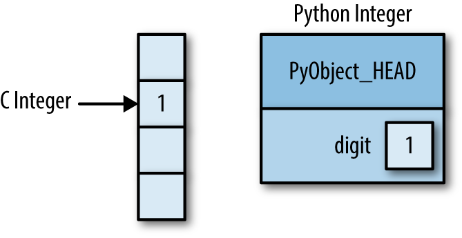
Here PyObject_HEAD is the part of the structure containing the
reference count, type code, and other pieces mentioned before.
Notice the difference here: a C integer is essentially a label for a position in memory whose bytes encode an integer value. A Python integer is a pointer to a position in memory containing all the Python object information, including the bytes that contain the integer value. This extra information in the Python integer structure is what allows Python to be coded so freely and dynamically. All this additional information in Python types comes at a cost, however, which becomes especially apparent in structures that combine many of these objects.
Let’s consider now what happens when we use a Python data structure that holds many Python objects. The standard mutable multielement container in Python is the list. We can create a list of integers as follows:
In[1]:L=list(range(10))L
Out[1]: [0, 1, 2, 3, 4, 5, 6, 7, 8, 9]
In[2]:type(L[0])
Out[2]: int
Or, similarly, a list of strings:
In[3]:L2=[str(c)forcinL]L2
Out[3]: ['0', '1', '2', '3', '4', '5', '6', '7', '8', '9']
In[4]:type(L2[0])
Out[4]: str
Because of Python’s dynamic typing, we can even create heterogeneous lists:
In[5]:L3=[True,"2",3.0,4][type(item)foriteminL3]
Out[5]: [bool, str, float, int]
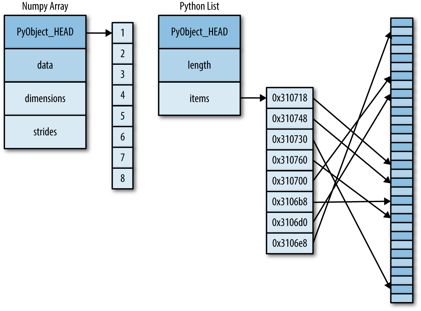
But this flexibility comes at a cost: to allow these flexible types, each item in the list must contain its own type info, reference count, and other information—that is, each item is a complete Python object. In the special case that all variables are of the same type, much of this information is redundant: it can be much more efficient to store data in a fixed-type array. The difference between a dynamic-type list and a fixed-type (NumPy-style) array is illustrated in Figure 2-2.
At the implementation level, the array essentially contains a single pointer to one contiguous block of data. The Python list, on the other hand, contains a pointer to a block of pointers, each of which in turn points to a full Python object like the Python integer we saw earlier. Again, the advantage of the list is flexibility: because each list element is a full structure containing both data and type information, the list can be filled with data of any desired type. Fixed-type NumPy-style arrays lack this flexibility, but are much more efficient for storing and manipulating data.
Python offers several different options for storing data in efficient,
fixed-type data buffers. The built-in array module (available since Python 3.3) can be used to create dense arrays of a uniform type:
In[6]:importarrayL=list(range(10))A=array.array('i',L)A
Out[6]: array('i', [0, 1, 2, 3, 4, 5, 6, 7, 8, 9])
Here 'i' is a type code indicating the contents are integers.
Much more useful, however, is the ndarray object of the NumPy package.
While Python’s array object provides efficient storage of array-based
data, NumPy adds to this efficient operations on that data. We will
explore these operations in later sections; here we’ll demonstrate
several ways of creating a NumPy array.
We’ll start with the standard NumPy import, under the alias np:
In[7]:importnumpyasnp
First, we can use np.array to create arrays from Python lists:
In[8]:# integer array:np.array([1,4,2,5,3])
Out[8]: array([1, 4, 2, 5, 3])
Remember that unlike Python lists, NumPy is constrained to arrays that all contain the same type. If types do not match, NumPy will upcast if possible (here, integers are upcast to floating point):
In[9]:np.array([3.14,4,2,3])
Out[9]: array([ 3.14, 4. , 2. , 3. ])
If we want to explicitly set the data type of the resulting array, we can
use the dtype keyword:
In[10]:np.array([1,2,3,4],dtype='float32')
Out[10]: array([ 1., 2., 3., 4.], dtype=float32)
Finally, unlike Python lists, NumPy arrays can explicitly be multidimensional; here’s one way of initializing a multidimensional array using a list of lists:
In[11]:# nested lists result in multidimensional arraysnp.array([range(i,i+3)foriin[2,4,6]])
Out[11]: array([[2, 3, 4],
[4, 5, 6],
[6, 7, 8]])
The inner lists are treated as rows of the resulting two-dimensional array.
Especially for larger arrays, it is more efficient to create arrays from scratch using routines built into NumPy. Here are several examples:
In[12]:# Create a length-10 integer array filled with zerosnp.zeros(10,dtype=int)
Out[12]: array([0, 0, 0, 0, 0, 0, 0, 0, 0, 0])
In[13]:# Create a 3x5 floating-point array filled with 1snp.ones((3,5),dtype=float)
Out[13]: array([[ 1., 1., 1., 1., 1.],
[ 1., 1., 1., 1., 1.],
[ 1., 1., 1., 1., 1.]])
In[14]:# Create a 3x5 array filled with 3.14np.full((3,5),3.14)
Out[14]: array([[ 3.14, 3.14, 3.14, 3.14, 3.14],
[ 3.14, 3.14, 3.14, 3.14, 3.14],
[ 3.14, 3.14, 3.14, 3.14, 3.14]])
In[15]:# Create an array filled with a linear sequence# Starting at 0, ending at 20, stepping by 2# (this is similar to the built-in range() function)np.arange(0,20,2)
Out[15]: array([ 0, 2, 4, 6, 8, 10, 12, 14, 16, 18])
In[16]:# Create an array of five values evenly spaced between 0 and 1np.linspace(0,1,5)
Out[16]: array([ 0. , 0.25, 0.5 , 0.75, 1. ])
In[17]:# Create a 3x3 array of uniformly distributed# random values between 0 and 1np.random.random((3,3))
Out[17]: array([[ 0.99844933, 0.52183819, 0.22421193],
[ 0.08007488, 0.45429293, 0.20941444],
[ 0.14360941, 0.96910973, 0.946117 ]])
In[18]:# Create a 3x3 array of normally distributed random values# with mean 0 and standard deviation 1np.random.normal(0,1,(3,3))
Out[18]: array([[ 1.51772646, 0.39614948, -0.10634696],
[ 0.25671348, 0.00732722, 0.37783601],
[ 0.68446945, 0.15926039, -0.70744073]])
In[19]:# Create a 3x3 array of random integers in the interval [0, 10)np.random.randint(0,10,(3,3))
Out[19]: array([[2, 3, 4],
[5, 7, 8],
[0, 5, 0]])
In[20]:# Create a 3x3 identity matrixnp.eye(3)
Out[20]: array([[ 1., 0., 0.],
[ 0., 1., 0.],
[ 0., 0., 1.]])
In[21]:# Create an uninitialized array of three integers# The values will be whatever happens to already exist at that# memory locationnp.empty(3)
Out[21]: array([ 1., 1., 1.])
NumPy arrays contain values of a single type, so it is important to have detailed knowledge of those types and their limitations. Because NumPy is built in C, the types will be familiar to users of C, Fortran, and other related languages.
The standard NumPy data types are listed in Table 2-1. Note that when constructing an array, you can specify them using a string:
np.zeros(10,dtype='int16')
Or using the associated NumPy object:
np.zeros(10,dtype=np.int16)
| Data type | Description |
|---|---|
|
Boolean (True or False) stored as a byte |
|
Default integer type (same as C |
|
Identical to C |
|
Integer used for indexing (same as C |
|
Byte (–128 to 127) |
|
Integer (–32768 to 32767) |
|
Integer (–2147483648 to 2147483647) |
|
Integer (–9223372036854775808 to 9223372036854775807) |
|
Unsigned integer (0 to 255) |
|
Unsigned integer (0 to 65535) |
|
Unsigned integer (0 to 4294967295) |
|
Unsigned integer (0 to 18446744073709551615) |
|
Shorthand for |
|
Half-precision float: sign bit, 5 bits exponent, 10 bits mantissa |
|
Single-precision float: sign bit, 8 bits exponent, 23 bits mantissa |
|
Double-precision float: sign bit, 11 bits exponent, 52 bits mantissa |
|
Shorthand for |
|
Complex number, represented by two 32-bit floats |
|
Complex number, represented by two 64-bit floats |
More advanced type specification is possible, such as specifying big or little endian numbers; for more information, refer to the NumPy documentation. NumPy also supports compound data types, which will be covered in “Structured Data: NumPy’s Structured Arrays”.
Data manipulation in Python is nearly synonymous with NumPy array manipulation: even newer tools like Pandas (Chapter 3) are built around the NumPy array. This section will present several examples using NumPy array manipulation to access data and subarrays, and to split, reshape, and join the arrays. While the types of operations shown here may seem a bit dry and pedantic, they comprise the building blocks of many other examples used throughout the book. Get to know them well!
We’ll cover a few categories of basic array manipulations here:
Determining the size, shape, memory consumption, and data types of arrays
Getting and setting the value of individual array elements
Getting and setting smaller subarrays within a larger array
Changing the shape of a given array
Combining multiple arrays into one, and splitting one array into many
First let’s discuss some useful array attributes. We’ll start by defining three random arrays: a one-dimensional, two-dimensional, and three-dimensional array. We’ll use NumPy’s random number generator, which we will seed with a set value in order to ensure that the same random arrays are generated each time this code is run:
In[1]:importnumpyasnpnp.random.seed(0)# seed for reproducibilityx1=np.random.randint(10,size=6)# One-dimensional arrayx2=np.random.randint(10,size=(3,4))# Two-dimensional arrayx3=np.random.randint(10,size=(3,4,5))# Three-dimensional array
Each array has attributes ndim (the number of dimensions),
shape (the size of each dimension), and size (the
total size of the array):
In[2]:("x3 ndim: ",x3.ndim)("x3 shape:",x3.shape)("x3 size: ",x3.size)
x3 ndim: 3 x3 shape: (3, 4, 5) x3 size: 60
Another useful attribute is the dtype, the data type of the
array (which we discussed previously in “Understanding Data Types in Python”):
In[3]:("dtype:",x3.dtype)
dtype: int64
Other attributes include itemsize, which lists the size (in bytes) of
each array element, and nbytes, which lists the total size (in bytes)
of the array:
In[4]:("itemsize:",x3.itemsize,"bytes")("nbytes:",x3.nbytes,"bytes")
itemsize: 8 bytes nbytes: 480 bytes
In general, we expect that nbytes is equal to itemsize times size.
If you are familiar with Python’s standard list indexing, indexing in NumPy will feel quite familiar. In a one-dimensional array, you can access the ith value (counting from zero) by specifying the desired index in square brackets, just as with Python lists:
In[5]:x1
Out[5]: array([5, 0, 3, 3, 7, 9])
In[6]:x1[0]
Out[6]: 5
In[7]:x1[4]
Out[7]: 7
To index from the end of the array, you can use negative indices:
In[8]:x1[-1]
Out[8]: 9
In[9]:x1[-2]
Out[9]: 7
In a multidimensional array, you access items using a comma-separated tuple of indices:
In[10]:x2
Out[10]: array([[3, 5, 2, 4],
[7, 6, 8, 8],
[1, 6, 7, 7]])
In[11]:x2[0,0]
Out[11]: 3
In[12]:x2[2,0]
Out[12]: 1
In[13]:x2[2,-1]
Out[13]: 7
You can also modify values using any of the above index notation:
In[14]:x2[0,0]=12x2
Out[14]: array([[12, 5, 2, 4],
[ 7, 6, 8, 8],
[ 1, 6, 7, 7]])
Keep in mind that, unlike Python lists, NumPy arrays have a fixed type. This means, for example, that if you attempt to insert a floating-point value to an integer array, the value will be silently truncated. Don’t be caught unaware by this behavior!
In[15]:x1[0]=3.14159# this will be truncated!x1
Out[15]: array([3, 0, 3, 3, 7, 9])
Just as we can use square brackets to access individual array elements,
we can also use them to access subarrays with the slice notation,
marked by the colon (:) character. The NumPy slicing syntax follows
that of the standard Python list; to access a slice of an array x, use this:
x[start:stop:step]
If any of these are unspecified, they default to the values start=0,
stop=size of dimension, step=1. We’ll take a look at accessing
subarrays in one dimension and in multiple dimensions.
In[16]:x=np.arange(10)x
Out[16]: array([0, 1, 2, 3, 4, 5, 6, 7, 8, 9])
In[17]:x[:5]# first five elements
Out[17]: array([0, 1, 2, 3, 4])
In[18]:x[5:]# elements after index 5
Out[18]: array([5, 6, 7, 8, 9])
In[19]:x[4:7]# middle subarray
Out[19]: array([4, 5, 6])
In[20]:x[::2]# every other element
Out[20]: array([0, 2, 4, 6, 8])
In[21]:x[1::2]# every other element, starting at index 1
Out[21]: array([1, 3, 5, 7, 9])
A potentially confusing case is when the step value is negative. In
this case, the defaults for start and stop are swapped. This becomes
a convenient way to reverse an array:
In[22]:x[::-1]# all elements, reversed
Out[22]: array([9, 8, 7, 6, 5, 4, 3, 2, 1, 0])
In[23]:x[5::-2]# reversed every other from index 5
Out[23]: array([5, 3, 1])
Multidimensional slices work in the same way, with multiple slices separated by commas. For example:
In[24]:x2
Out[24]: array([[12, 5, 2, 4],
[ 7, 6, 8, 8],
[ 1, 6, 7, 7]])
In[25]:x2[:2,:3]# two rows, three columns
Out[25]: array([[12, 5, 2],
[ 7, 6, 8]])
In[26]:x2[:3,::2]# all rows, every other column
Out[26]: array([[12, 2],
[ 7, 8],
[ 1, 7]])
Finally, subarray dimensions can even be reversed together:
In[27]:x2[::-1,::-1]
Out[27]: array([[ 7, 7, 6, 1],
[ 8, 8, 6, 7],
[ 4, 2, 5, 12]])
One commonly needed routine is accessing single rows or columns of an
array. You can do this by combining indexing and slicing, using an
empty slice marked by a single colon (:):
In[28]:(x2[:,0])# first column of x2
[12 7 1]
In[29]:(x2[0,:])# first row of x2
[12 5 2 4]
In the case of row access, the empty slice can be omitted for a more compact syntax:
In[30]:(x2[0])# equivalent to x2[0, :]
[12 5 2 4]
One important—and extremely useful—thing to know about array slices is that they return views rather than copies of the array data. This is one area in which NumPy array slicing differs from Python list slicing: in lists, slices will be copies. Consider our two-dimensional array from before:
In[31]:(x2)
[[12 5 2 4] [ 7 6 8 8] [ 1 6 7 7]]
Let’s extract a 2×2 subarray from this:
In[32]:x2_sub=x2[:2,:2](x2_sub)
[[12 5] [ 7 6]]
Now if we modify this subarray, we’ll see that the original array is changed! Observe:
In[33]:x2_sub[0,0]=99(x2_sub)
[[99 5] [ 7 6]]
In[34]:(x2)
[[99 5 2 4] [ 7 6 8 8] [ 1 6 7 7]]
This default behavior is actually quite useful: it means that when we work with large datasets, we can access and process pieces of these datasets without the need to copy the underlying data buffer.
Despite the nice features of array views, it is sometimes useful to
instead explicitly copy the data within an array or a subarray. This can
be most easily done with the copy() method:
In[35]:x2_sub_copy=x2[:2,:2].copy()(x2_sub_copy)
[[99 5] [ 7 6]]
If we now modify this subarray, the original array is not touched:
In[36]:x2_sub_copy[0,0]=42(x2_sub_copy)
[[42 5] [ 7 6]]
In[37]:(x2)
[[99 5 2 4] [ 7 6 8 8] [ 1 6 7 7]]
Another useful type of operation is reshaping of arrays. The most
flexible way of doing this is with the reshape() method. For example, if
you want to put the numbers 1 through 9 in a 3×3 grid, you can do the
following:
In[38]:grid=np.arange(1,10).reshape((3,3))(grid)
[[1 2 3] [4 5 6] [7 8 9]]
Note that for this to work, the size of the initial array must match the
size of the reshaped array. Where possible, the reshape method will
use a no-copy view of the initial array, but with noncontiguous memory
buffers this is not always the case.
Another common reshaping pattern is the conversion of a one-dimensional array into a
two-dimensional row or column matrix. You can do this with the reshape method, or
more easily by making use of the newaxis keyword within a slice
operation:
In[39]:x=np.array([1,2,3])# row vector via reshapex.reshape((1,3))
Out[39]: array([[1, 2, 3]])
In[40]:# row vector via newaxisx[np.newaxis,:]
Out[40]: array([[1, 2, 3]])
In[41]:# column vector via reshapex.reshape((3,1))
Out[41]: array([[1],
[2],
[3]])
In[42]:# column vector via newaxisx[:,np.newaxis]
Out[42]: array([[1],
[2],
[3]])
We will see this type of transformation often throughout the remainder of the book.
All of the preceding routines worked on single arrays. It’s also possible to combine multiple arrays into one, and to conversely split a single array into multiple arrays. We’ll take a look at those operations here.
Concatenation, or joining of two arrays in NumPy, is primarily
accomplished through the routines np.concatenate, np.vstack, and
np.hstack. np.concatenate takes a tuple or list of arrays as its first
argument, as we can see here:
In[43]:x=np.array([1,2,3])y=np.array([3,2,1])np.concatenate([x,y])
Out[43]: array([1, 2, 3, 3, 2, 1])
You can also concatenate more than two arrays at once:
In[44]:z=[99,99,99](np.concatenate([x,y,z]))
[ 1 2 3 3 2 1 99 99 99]
np.concatenate can also be used for two-dimensional arrays:
In[45]:grid=np.array([[1,2,3],[4,5,6]])
In[46]:# concatenate along the first axisnp.concatenate([grid,grid])
Out[46]: array([[1, 2, 3],
[4, 5, 6],
[1, 2, 3],
[4, 5, 6]])
In[47]:# concatenate along the second axis (zero-indexed)np.concatenate([grid,grid],axis=1)
Out[47]: array([[1, 2, 3, 1, 2, 3],
[4, 5, 6, 4, 5, 6]])
For working with arrays of mixed dimensions, it can be clearer to use
the np.vstack (vertical stack) and np.hstack (horizontal stack)
functions:
In[48]:x=np.array([1,2,3])grid=np.array([[9,8,7],[6,5,4]])# vertically stack the arraysnp.vstack([x,grid])
Out[48]: array([[1, 2, 3],
[9, 8, 7],
[6, 5, 4]])
In[49]:# horizontally stack the arraysy=np.array([[99],[99]])np.hstack([grid,y])
Out[49]: array([[ 9, 8, 7, 99],
[ 6, 5, 4, 99]])
Similarly, np.dstack will stack arrays along the third axis.
The opposite of concatenation is splitting, which is implemented by the
functions np.split, np.hsplit, and np.vsplit. For each of these,
we can pass a list of indices giving the split points:
In[50]:x=[1,2,3,99,99,3,2,1]x1,x2,x3=np.split(x,[3,5])(x1,x2,x3)
[1 2 3] [99 99] [3 2 1]
Notice that N split points lead to N + 1 subarrays. The related
functions np.hsplit and np.vsplit are similar:
In[51]:grid=np.arange(16).reshape((4,4))grid
Out[51]: array([[ 0, 1, 2, 3],
[ 4, 5, 6, 7],
[ 8, 9, 10, 11],
[12, 13, 14, 15]])
In[52]:upper,lower=np.vsplit(grid,[2])(upper)(lower)
[[0 1 2 3] [4 5 6 7]] [[ 8 9 10 11] [12 13 14 15]]
In[53]:left,right=np.hsplit(grid,[2])(left)(right)
[[ 0 1] [ 4 5] [ 8 9] [12 13]] [[ 2 3] [ 6 7] [10 11] [14 15]]
Similarly, np.dsplit will split arrays along the third axis.
Up until now, we have been discussing some of the basic nuts and bolts of NumPy; in the next few sections, we will dive into the reasons that NumPy is so important in the Python data science world. Namely, it provides an easy and flexible interface to optimized computation with arrays of data.
Computation on NumPy arrays can be very fast, or it can be very slow. The key to making it fast is to use vectorized operations, generally implemented through NumPy’s universal functions (ufuncs). This section motivates the need for NumPy’s ufuncs, which can be used to make repeated calculations on array elements much more efficient. It then introduces many of the most common and useful arithmetic ufuncs available in the NumPy package.
Python’s default implementation (known as CPython) does some operations very slowly. This is in part due to the dynamic, interpreted nature of the language: the fact that types are flexible, so that sequences of operations cannot be compiled down to efficient machine code as in languages like C and Fortran. Recently there have been various attempts to address this weakness: well-known examples are the PyPy project, a just-in-time compiled implementation of Python; the Cython project, which converts Python code to compilable C code; and the Numba project, which converts snippets of Python code to fast LLVM bytecode. Each of these has its strengths and weaknesses, but it is safe to say that none of the three approaches has yet surpassed the reach and popularity of the standard CPython engine.
The relative sluggishness of Python generally manifests itself in situations where many small operations are being repeated—for instance, looping over arrays to operate on each element. For example, imagine we have an array of values and we’d like to compute the reciprocal of each. A straightforward approach might look like this:
In[1]:importnumpyasnpnp.random.seed(0)defcompute_reciprocals(values):output=np.empty(len(values))foriinrange(len(values)):output[i]=1.0/values[i]returnoutputvalues=np.random.randint(1,10,size=5)compute_reciprocals(values)
Out[1]: array([ 0.16666667, 1. , 0.25 , 0.25 , 0.125 ])
This implementation probably feels fairly natural to someone from, say,
a C or Java background. But if we measure the execution time of this
code for a large input, we see that this operation is very slow, perhaps
surprisingly so! We’ll benchmark this with IPython’s %timeit magic
(discussed in “Profiling and Timing Code”):
In[2]:big_array=np.random.randint(1,100,size=1000000)%timeitcompute_reciprocals(big_array)
1 loop, best of 3: 2.91 s per loop
It takes several seconds to compute these million operations and to store the result! When even cell phones have processing speeds measured in Giga-FLOPS (i.e., billions of numerical operations per second), this seems almost absurdly slow. It turns out that the bottleneck here is not the operations themselves, but the type-checking and function dispatches that CPython must do at each cycle of the loop. Each time the reciprocal is computed, Python first examines the object’s type and does a dynamic lookup of the correct function to use for that type. If we were working in compiled code instead, this type specification would be known before the code executes and the result could be computed much more efficiently.
For many types of operations, NumPy provides a convenient interface into just this kind of statically typed, compiled routine. This is known as a vectorized operation. You can accomplish this by simply performing an operation on the array, which will then be applied to each element. This vectorized approach is designed to push the loop into the compiled layer that underlies NumPy, leading to much faster execution.
Compare the results of the following two:
In[3]:(compute_reciprocals(values))(1.0/values)
[ 0.16666667 1. 0.25 0.25 0.125 ] [ 0.16666667 1. 0.25 0.25 0.125 ]
Looking at the execution time for our big array, we see that it completes orders of magnitude faster than the Python loop:
In[4]:%timeit(1.0/big_array)
100 loops, best of 3: 4.6 ms per loop
Vectorized operations in NumPy are implemented via ufuncs, whose main purpose is to quickly execute repeated operations on values in NumPy arrays. Ufuncs are extremely flexible—before we saw an operation between a scalar and an array, but we can also operate between two arrays:
In[5]:np.arange(5)/np.arange(1,6)
Out[5]: array([ 0. , 0.5 , 0.66666667, 0.75 , 0.8 ])
And ufunc operations are not limited to one-dimensional arrays—they can act on multidimensional arrays as well:
In[6]:x=np.arange(9).reshape((3,3))2**x
Out[6]: array([[ 1, 2, 4],
[ 8, 16, 32],
[ 64, 128, 256]])
Computations using vectorization through ufuncs are nearly always more efficient than their counterpart implemented through Python loops, especially as the arrays grow in size. Any time you see such a loop in a Python script, you should consider whether it can be replaced with a vectorized expression.
Ufuncs exist in two flavors: unary ufuncs, which operate on a single input, and binary ufuncs, which operate on two inputs. We’ll see examples of both these types of functions here.
NumPy’s ufuncs feel very natural to use because they make use of Python’s native arithmetic operators. The standard addition, subtraction, multiplication, and division can all be used:
In[7]:x=np.arange(4)("x =",x)("x + 5 =",x+5)("x - 5 =",x-5)("x * 2 =",x*2)("x / 2 =",x/2)("x // 2 =",x//2)# floor division
x = [0 1 2 3] x + 5 = [5 6 7 8] x - 5 = [-5 -4 -3 -2] x * 2 = [0 2 4 6] x / 2 = [ 0. 0.5 1. 1.5] x // 2 = [0 0 1 1]
There is also a unary ufunc for negation, a ** operator for
exponentiation, and a % operator for modulus:
In[8]:("-x = ",-x)("x ** 2 = ",x**2)("x % 2 = ",x%2)
-x = [ 0 -1 -2 -3] x ** 2 = [0 1 4 9] x % 2 = [0 1 0 1]
In addition, these can be strung together however you wish, and the standard order of operations is respected:
In[9]:-(0.5*x+1)**2
Out[9]: array([-1. , -2.25, -4. , -6.25])
All of these arithmetic operations are simply convenient wrappers
around specific functions built into NumPy; for example, the +
operator is a wrapper for the add function:
In[10]:np.add(x,2)
Out[10]: array([2, 3, 4, 5])
Table 2-2 lists the arithmetic operators implemented in NumPy.
| Operator | Equivalent ufunc | Description |
|---|---|---|
|
|
Addition (e.g., |
|
|
Subtraction (e.g., |
|
|
Unary negation (e.g., |
|
|
Multiplication (e.g., |
|
|
Division (e.g., |
|
|
Floor division (e.g., |
|
|
Exponentiation (e.g., |
|
|
Modulus/remainder (e.g., |
Additionally there are Boolean/bitwise operators; we will explore these in “Comparisons, Masks, and Boolean Logic”.
Just as NumPy understands Python’s built-in arithmetic operators, it also understands Python’s built-in absolute value function:
In[11]:x=np.array([-2,-1,0,1,2])abs(x)
Out[11]: array([2, 1, 0, 1, 2])
The corresponding NumPy ufunc is np.absolute, which is also available
under the alias np.abs:
In[12]:np.absolute(x)
Out[12]: array([2, 1, 0, 1, 2])
In[13]:np.abs(x)
Out[13]: array([2, 1, 0, 1, 2])
This ufunc can also handle complex data, in which the absolute value returns the magnitude:
In[14]:x=np.array([3-4j,4-3j,2+0j,0+1j])np.abs(x)
Out[14]: array([ 5., 5., 2., 1.])
NumPy provides a large number of useful ufuncs, and some of the most useful for the data scientist are the trigonometric functions. We’ll start by defining an array of angles:
In[15]:theta=np.linspace(0,np.pi,3)
Now we can compute some trigonometric functions on these values:
In[16]:("theta = ",theta)("sin(theta) = ",np.sin(theta))("cos(theta) = ",np.cos(theta))("tan(theta) = ",np.tan(theta))
theta = [ 0. 1.57079633 3.14159265] sin(theta) = [ 0.00000000e+00 1.00000000e+00 1.22464680e-16] cos(theta) = [ 1.00000000e+00 6.12323400e-17 -1.00000000e+00] tan(theta) = [ 0.00000000e+00 1.63312394e+16 -1.22464680e-16]
The values are computed to within machine precision, which is why values that should be zero do not always hit exactly zero. Inverse trigonometric functions are also available:
In[17]:x=[-1,0,1]("x = ",x)("arcsin(x) = ",np.arcsin(x))("arccos(x) = ",np.arccos(x))("arctan(x) = ",np.arctan(x))
x = [-1, 0, 1] arcsin(x) = [-1.57079633 0. 1.57079633] arccos(x) = [ 3.14159265 1.57079633 0. ] arctan(x) = [-0.78539816 0. 0.78539816]
Another common type of operation available in a NumPy ufunc are the exponentials:
In[18]:x=[1,2,3]("x =",x)("e^x =",np.exp(x))("2^x =",np.exp2(x))("3^x =",np.power(3,x))
x = [1, 2, 3] e^x = [ 2.71828183 7.3890561 20.08553692] 2^x = [ 2. 4. 8.] 3^x = [ 3 9 27]
The inverse of the exponentials, the logarithms, are also available. The
basic np.log gives the natural logarithm; if you prefer to compute the
base-2 logarithm or the base-10 logarithm, these are available as well:
In[19]:x=[1,2,4,10]("x =",x)("ln(x) =",np.log(x))("log2(x) =",np.log2(x))("log10(x) =",np.log10(x))
x = [1, 2, 4, 10] ln(x) = [ 0. 0.69314718 1.38629436 2.30258509] log2(x) = [ 0. 1. 2. 3.32192809] log10(x) = [ 0. 0.30103 0.60205999 1. ]
There are also some specialized versions that are useful for maintaining precision with very small input:
In[20]:x=[0,0.001,0.01,0.1]("exp(x) - 1 =",np.expm1(x))("log(1 + x) =",np.log1p(x))
exp(x) - 1 = [ 0. 0.0010005 0.01005017 0.10517092] log(1 + x) = [ 0. 0.0009995 0.00995033 0.09531018]
When x is very small, these functions give more precise values than if
the raw np.log or np.exp were used.
NumPy has many more ufuncs available, including hyperbolic trig functions, bitwise arithmetic, comparison operators, conversions from radians to degrees, rounding and remainders, and much more. A look through the NumPy documentation reveals a lot of interesting functionality.
Another excellent source for more specialized and obscure ufuncs is the submodule scipy.special. If you want to compute some obscure
mathematical function on your data, chances are it is implemented in
scipy.special. There are far too many functions to list them all,
but the following snippet shows a couple that might come up in a statistics context:
In[21]:fromscipyimportspecial
In[22]:# Gamma functions (generalized factorials) and related functionsx=[1,5,10]("gamma(x) =",special.gamma(x))("ln|gamma(x)| =",special.gammaln(x))("beta(x, 2) =",special.beta(x,2))
gamma(x) = [ 1.00000000e+00 2.40000000e+01 3.62880000e+05] ln|gamma(x)| = [ 0. 3.17805383 12.80182748] beta(x, 2) = [ 0.5 0.03333333 0.00909091]
In[23]:# Error function (integral of Gaussian)# its complement, and its inversex=np.array([0,0.3,0.7,1.0])("erf(x) =",special.erf(x))("erfc(x) =",special.erfc(x))("erfinv(x) =",special.erfinv(x))
erf(x) = [ 0. 0.32862676 0.67780119 0.84270079] erfc(x) = [ 1. 0.67137324 0.32219881 0.15729921] erfinv(x) = [ 0. 0.27246271 0.73286908 inf]
There are many, many more ufuncs available in both NumPy and
scipy.special. Because the documentation of these packages is
available online, a web search along the lines of “gamma function
python” will generally find the relevant information.
Many NumPy users make use of ufuncs without ever learning their full set of features. We’ll outline a few specialized features of ufuncs here.
For large calculations, it is sometimes useful to be able to specify the
array where the result of the calculation will be stored. Rather than
creating a temporary array, you can use this to write computation
results directly to the memory location where you’d like them to be. For
all ufuncs, you can do this using the out argument of the function:
In[24]:x=np.arange(5)y=np.empty(5)np.multiply(x,10,out=y)(y)
[ 0. 10. 20. 30. 40.]
This can even be used with array views. For example, we can write the results of a computation to every other element of a specified array:
In[25]:y=np.zeros(10)np.power(2,x,out=y[::2])(y)
[ 1. 0. 2. 0. 4. 0. 8. 0. 16. 0.]
If we had instead written y[::2] = 2 ** x, this would have resulted in
the creation of a temporary array to hold the results of 2 ** x,
followed by a second operation copying those values into the y array.
This doesn’t make much of a difference for such a small computation, but
for very large arrays the memory savings from careful use of the out
argument can be significant.
For binary ufuncs, there are some interesting aggregates that can be
computed directly from the object. For example, if we’d like to reduce
an array with a particular operation, we can use the reduce method of
any ufunc. A reduce repeatedly applies a given operation to the elements
of an array until only a single result remains.
For example, calling reduce on the add ufunc returns the sum of all
elements in the array:
In[26]:x=np.arange(1,6)np.add.reduce(x)
Out[26]: 15
Similarly, calling reduce on the multiply ufunc results in the
product of all array elements:
In[27]:np.multiply.reduce(x)
Out[27]: 120
If we’d like to store all the intermediate results of the computation,
we can instead use accumulate:
In[28]:np.add.accumulate(x)
Out[28]: array([ 1, 3, 6, 10, 15])
In[29]:np.multiply.accumulate(x)
Out[29]: array([ 1, 2, 6, 24, 120])
Note that for these particular cases, there are dedicated NumPy
functions to compute the results (np.sum, np.prod, np.cumsum,
np.cumprod), which we’ll explore in “Aggregations: Min, Max, and Everything in Between”.
Finally, any ufunc can compute the output of all pairs of two different
inputs using the outer method. This allows you, in one line, to do
things like create a multiplication table:
In[30]:x=np.arange(1,6)np.multiply.outer(x,x)
Out[30]: array([[ 1, 2, 3, 4, 5],
[ 2, 4, 6, 8, 10],
[ 3, 6, 9, 12, 15],
[ 4, 8, 12, 16, 20],
[ 5, 10, 15, 20, 25]])
The ufunc.at and
ufunc.reduceat methods, which we’ll explore in
“Fancy Indexing”, are very helpful as well.
Another extremely useful feature of ufuncs is the ability to operate between arrays of different sizes and shapes, a set of operations known as broadcasting. This subject is important enough that we will devote a whole section to it (see “Computation on Arrays: Broadcasting”).
More information on universal functions (including the full list of available functions) can be found on the NumPy and SciPy documentation websites.
Recall that you can also access information directly from within IPython
by importing the packages and using IPython’s tab-completion and
help (?) functionality, as described in “Help and Documentation in IPython”.
Often when you are faced with a large amount of data, a first step is to compute summary statistics for the data in question. Perhaps the most common summary statistics are the mean and standard deviation, which allow you to summarize the “typical” values in a dataset, but other aggregates are useful as well (the sum, product, median, minimum and maximum, quantiles, etc.).
NumPy has fast built-in aggregation functions for working on arrays; we’ll discuss and demonstrate some of them here.
As a quick example, consider computing the sum of all values in an
array. Python itself can do this using the built-in sum function:
In[1]:importnumpyasnp
In[2]:L=np.random.random(100)sum(L)
Out[2]: 55.61209116604941
The syntax is quite similar to that of NumPy’s sum function, and the
result is the same in the simplest case:
In[3]:np.sum(L)
Out[3]: 55.612091166049424
However, because it executes the operation in compiled code, NumPy’s version of the operation is computed much more quickly:
In[4]:big_array=np.random.rand(1000000)%timeitsum(big_array)%timeitnp.sum(big_array)
10 loops, best of 3: 104 ms per loop 1000 loops, best of 3: 442 µs per loop
Be careful, though: the sum function and the np.sum function are not
identical, which can sometimes lead to confusion! In particular, their
optional arguments have different meanings, and np.sum is aware of
multiple array dimensions, as we will see in the following section.
Similarly, Python has built-in min and max functions, used to find
the minimum value and maximum value of any given array:
In[5]:min(big_array),max(big_array)
Out[5]: (1.1717128136634614e-06, 0.9999976784968716)
NumPy’s corresponding functions have similar syntax, and again operate much more quickly:
In[6]:np.min(big_array),np.max(big_array)
Out[6]: (1.1717128136634614e-06, 0.9999976784968716)
In[7]:%timeitmin(big_array)%timeitnp.min(big_array)
10 loops, best of 3: 82.3 ms per loop 1000 loops, best of 3: 497 µs per loop
For min, max, sum, and several other NumPy aggregates, a shorter
syntax is to use methods of the array object itself:
In[8]:(big_array.min(),big_array.max(),big_array.sum())
1.17171281366e-06 0.999997678497 499911.628197
Whenever possible, make sure that you are using the NumPy version of these aggregates when operating on NumPy arrays!
One common type of aggregation operation is an aggregate along a row or column. Say you have some data stored in a two-dimensional array:
In[9]:M=np.random.random((3,4))(M)
[[ 0.8967576 0.03783739 0.75952519 0.06682827] [ 0.8354065 0.99196818 0.19544769 0.43447084] [ 0.66859307 0.15038721 0.37911423 0.6687194 ]]
By default, each NumPy aggregation function will return the aggregate over the entire array:
In[10]:M.sum()
Out[10]: 6.0850555667307118
Aggregation functions take an additional argument specifying the axis
along which the aggregate is computed. For example, we can find the
minimum value within each column by specifying axis=0:
In[11]:M.min(axis=0)
Out[11]: array([ 0.66859307, 0.03783739, 0.19544769, 0.06682827])
The function returns four values, corresponding to the four columns of numbers.
Similarly, we can find the maximum value within each row:
In[12]:M.max(axis=1)
Out[12]: array([ 0.8967576 , 0.99196818, 0.6687194 ])
The way the axis is specified here can be confusing to users coming from
other languages. The axis keyword specifies the dimension of the
array that will be collapsed, rather than the dimension that will be
returned. So specifying axis=0 means that the first axis will be
collapsed: for two-dimensional arrays, this means that values within
each column will be aggregated.
NumPy provides many other aggregation functions, but we won’t discuss them in detail here. Additionally, most aggregates have a NaN-safe counterpart that computes the result while ignoring missing values, which are
marked by the special IEEE floating-point NaN value (for a fuller
discussion of missing data, see “Handling Missing Data”). Some of these NaN-safe functions were not added
until NumPy 1.8, so they will not be available in older NumPy versions.
Table 2-3 provides a list of useful aggregation functions available in NumPy.
| Function Name | NaN-safe Version | Description |
|---|---|---|
|
|
Compute sum of elements |
|
|
Compute product of elements |
|
|
Compute median of elements |
|
|
Compute standard deviation |
|
|
Compute variance |
|
|
Find minimum value |
|
|
Find maximum value |
|
|
Find index of minimum value |
|
|
Find index of maximum value |
|
|
Compute median of elements |
|
|
Compute rank-based statistics of elements |
|
N/A |
Evaluate whether any elements are true |
|
N/A |
Evaluate whether all elements are true |
We will see these aggregates often throughout the rest of the book.
Aggregates available in NumPy can be extremely useful for summarizing a set of values. As a simple example, let’s consider the heights of all US presidents. This data is available in the file president_heights.csv, which is a simple comma-separated list of labels and values:
In[13]:!head-4data/president_heights.csv
order,name,height(cm) 1,George Washington,189 2,John Adams,170 3,Thomas Jefferson,189
We’ll use the Pandas package, which we’ll explore more fully in Chapter 3, to read the file and extract this information (note that the heights are measured in centimeters):
In[14]:importpandasaspddata=pd.read_csv('data/president_heights.csv')heights=np.array(data['height(cm)'])(heights)
[189 170 189 163 183 171 185 168 173 183 173 173 175 178 183 193 178 173 174 183 183 168 170 178 182 180 183 178 182 188 175 179 183 193 182 183 177 185 188 188 182 185]
Now that we have this data array, we can compute a variety of summary statistics:
In[15]:("Mean height: ",heights.mean())("Standard deviation:",heights.std())("Minimum height: ",heights.min())("Maximum height: ",heights.max())
Mean height: 179.738095238 Standard deviation: 6.93184344275 Minimum height: 163 Maximum height: 193
Note that in each case, the aggregation operation reduced the entire array to a single summarizing value, which gives us information about the distribution of values. We may also wish to compute quantiles:
In[16]:("25th percentile: ",np.percentile(heights,25))("Median: ",np.median(heights))("75th percentile: ",np.percentile(heights,75))
25th percentile: 174.25 Median: 182.0 75th percentile: 183.0
We see that the median height of US presidents is 182 cm, or just shy of six feet.
Of course, sometimes it’s more useful to see a visual representation of this data, which we can accomplish using tools in Matplotlib (we’ll discuss Matplotlib more fully in Chapter 4). For example, this code generates the chart shown in Figure 2-3:
In[17]:%matplotlibinlineimportmatplotlib.pyplotaspltimportseaborn;seaborn.set()# set plot style
In[18]:plt.hist(heights)plt.title('Height Distribution of US Presidents')plt.xlabel('height (cm)')plt.ylabel('number');
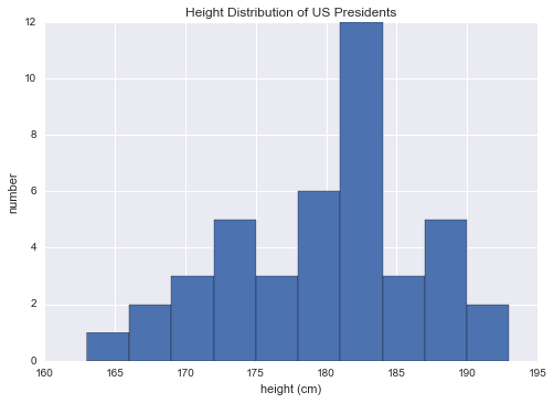
These aggregates are some of the fundamental pieces of exploratory data analysis that we’ll explore in more depth in later chapters of the book.
We saw in the previous section how NumPy’s universal functions can be used to vectorize operations and thereby remove slow Python loops. Another means of vectorizing operations is to use NumPy’s broadcasting functionality. Broadcasting is simply a set of rules for applying binary ufuncs (addition, subtraction, multiplication, etc.) on arrays of different sizes.
Recall that for arrays of the same size, binary operations are performed on an element-by-element basis:
In[1]:importnumpyasnp
In[2]:a=np.array([0,1,2])b=np.array([5,5,5])a+b
Out[2]: array([5, 6, 7])
Broadcasting allows these types of binary operations to be performed on arrays of different sizes—for example, we can just as easily add a scalar (think of it as a zero-dimensional array) to an array:
In[3]:a+5
Out[3]: array([5, 6, 7])
We can think of this as an operation that stretches or duplicates the
value 5 into the array [5, 5, 5], and adds the results. The
advantage of NumPy’s broadcasting is that this duplication of values
does not actually take place, but it is a useful mental model as we
think about broadcasting.
We can similarly extend this to arrays of higher dimension. Observe the result when we add a one-dimensional array to a two-dimensional array:
In[4]:M=np.ones((3,3))M
Out[4]: array([[ 1., 1., 1.],
[ 1., 1., 1.],
[ 1., 1., 1.]])
In[5]:M+a
Out[5]: array([[ 1., 2., 3.],
[ 1., 2., 3.],
[ 1., 2., 3.]])
Here the one-dimensional array a is stretched, or broadcast, across the
second dimension in order to match the shape of M.
While these examples are relatively easy to understand, more complicated cases can involve broadcasting of both arrays. Consider the following example:
In[6]:a=np.arange(3)b=np.arange(3)[:,np.newaxis](a)(b)
[0 1 2] [[0] [1] [2]]
In[7]:a+b
Out[7]: array([[0, 1, 2],
[1, 2, 3],
[2, 3, 4]])
Just as before we stretched or broadcasted one value to match the shape
of the other, here we’ve stretched both a and b to match a common
shape, and the result is a two-dimensional array! The geometry of these examples is visualized in Figure 2-4.1
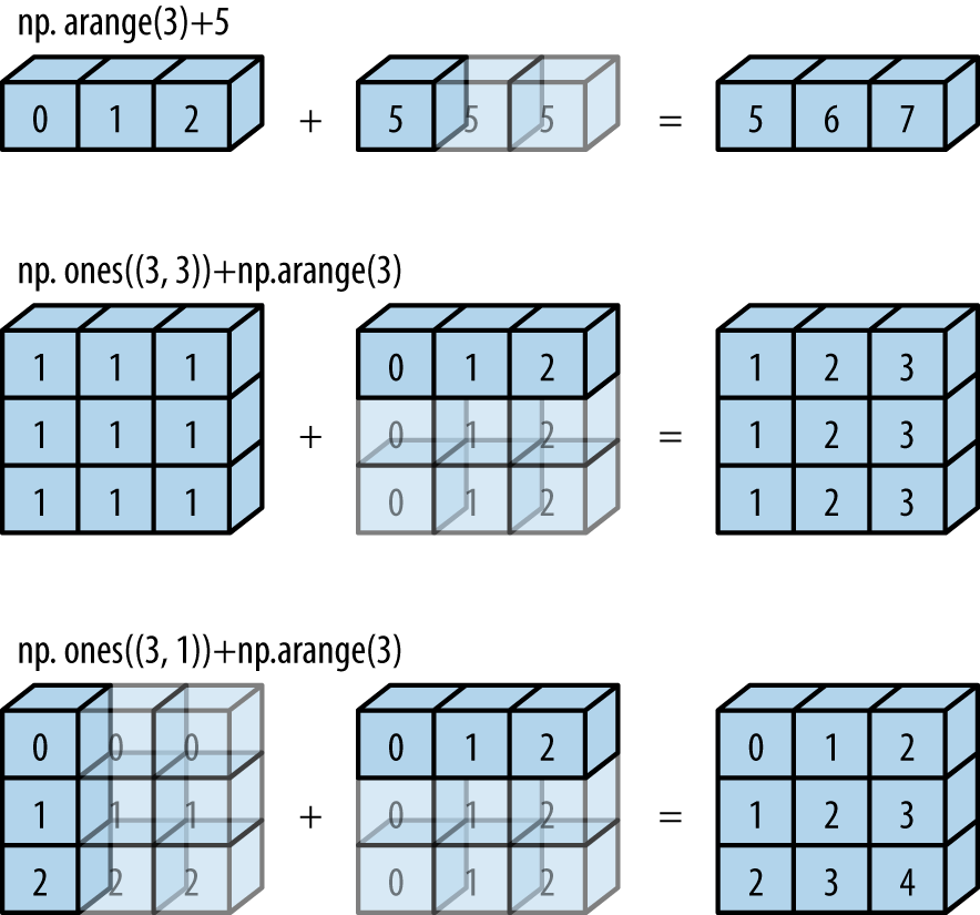
The light boxes represent the broadcasted values: again, this extra memory is not actually allocated in the course of the operation, but it can be useful conceptually to imagine that it is.
Broadcasting in NumPy follows a strict set of rules to determine the interaction between the two arrays:
Rule 1: If the two arrays differ in their number of dimensions, the shape of the one with fewer dimensions is padded with ones on its leading (left) side.
Rule 2: If the shape of the two arrays does not match in any dimension, the array with shape equal to 1 in that dimension is stretched to match the other shape.
Rule 3: If in any dimension the sizes disagree and neither is equal to 1, an error is raised.
To make these rules clear, let’s consider a few examples in detail.
Let’s look at adding a two-dimensional array to a one-dimensional array:
In[8]:M=np.ones((2,3))a=np.arange(3)
Let’s consider an operation on these two arrays. The shapes of the arrays are:
M.shape = (2, 3)a.shape = (3,)We see by rule 1 that the array a has fewer dimensions, so we pad
it on the left with ones:
M.shape -> (2, 3)a.shape -> (1, 3)By rule 2, we now see that the first dimension disagrees, so we stretch this dimension to match:
M.shape -> (2, 3)a.shape -> (2, 3)The shapes match, and we see that the final shape will be (2, 3):
In[9]:M+a
Out[9]: array([[ 1., 2., 3.],
[ 1., 2., 3.]])
Let’s take a look at an example where both arrays need to be broadcast:
In[10]:a=np.arange(3).reshape((3,1))b=np.arange(3)
Again, we’ll start by writing out the shape of the arrays:
a.shape = (3, 1)b.shape = (3,)Rule 1 says we must pad the shape of b with ones:
a.shape -> (3, 1)b.shape -> (1, 3)And rule 2 tells us that we upgrade each of these ones to match the corresponding size of the other array:
a.shape -> (3, 3)b.shape -> (3, 3)Because the result matches, these shapes are compatible. We can see this here:
In[11]:a+b
Out[11]: array([[0, 1, 2],
[1, 2, 3],
[2, 3, 4]])
Now let’s take a look at an example in which the two arrays are not compatible:
In[12]:M=np.ones((3,2))a=np.arange(3)
This is just a slightly different situation than in the first example: the
matrix M is transposed. How does this affect the calculation? The
shapes of the arrays are:
M.shape = (3, 2)a.shape = (3,)Again, rule 1 tells us that we must pad the shape of a with ones:
M.shape -> (3, 2)a.shape -> (1, 3)By rule 2, the first dimension of a is stretched to match that of M:
M.shape -> (3, 2)a.shape -> (3, 3)Now we hit rule 3—the final shapes do not match, so these two arrays are incompatible, as we can observe by attempting this operation:
In[13]:M+a
--------------------------------------------------------------------------- ValueError Traceback (most recent call last) <ipython-input-13-9e16e9f98da6> in <module>() ----> 1 M + a ValueError: operands could not be broadcast together with shapes (3,2) (3,)
Note the potential confusion here: you could imagine making a and M
compatible by, say, padding a’s shape with ones on the right rather
than the left. But this is not how the broadcasting rules work! That
sort of flexibility might be useful in some cases, but it would lead to
potential areas of ambiguity. If right-side padding is what you’d like,
you can do this explicitly by reshaping the array (we’ll use the
np.newaxis keyword introduced in “The Basics of NumPy Arrays”):
In[14]:a[:,np.newaxis].shape
Out[14]: (3, 1)
In[15]:M+a[:,np.newaxis]
Out[15]: array([[ 1., 1.],
[ 2., 2.],
[ 3., 3.]])
Also note that while we’ve been focusing on the + operator here,
these broadcasting rules apply to any binary ufunc. For example,
here is the logaddexp(a, b) function, which computes
log(exp(a) + exp(b)) with more precision than the naive approach:
In[16]:np.logaddexp(M,a[:,np.newaxis])
Out[16]: array([[ 1.31326169, 1.31326169],
[ 1.69314718, 1.69314718],
[ 2.31326169, 2.31326169]])
For more information on the many available universal functions, refer to “Computation on NumPy Arrays: Universal Functions”.
Broadcasting operations form the core of many examples we’ll see throughout this book. We’ll now take a look at a couple simple examples of where they can be useful.
In the previous section, we saw that ufuncs allow a NumPy user to remove the need to explicitly write slow Python loops. Broadcasting extends this ability. One commonly seen example is centering an array of data. Imagine you have an array of 10 observations, each of which consists of 3 values. Using the standard convention (see “Data Representation in Scikit-Learn”), we’ll store this in a 10×3 array:
In[17]:X=np.random.random((10,3))
We can compute the mean of each feature using the mean aggregate
across the first dimension:
In[18]:Xmean=X.mean(0)Xmean
Out[18]: array([ 0.53514715, 0.66567217, 0.44385899])
And now we can center the X array by subtracting the mean (this is a
broadcasting operation):
In[19]:X_centered=X-Xmean
To double-check that we’ve done this correctly, we can check that the centered array has near zero mean:
In[20]:X_centered.mean(0)
Out[20]: array([ 2.22044605e-17, -7.77156117e-17, -1.66533454e-17])
To within-machine precision, the mean is now zero.
One place that broadcasting is very useful is in displaying images based on two-dimensional functions. If we want to define a function z = f(x, y), broadcasting can be used to compute the function across the grid:
In[21]:# x and y have 50 steps from 0 to 5x=np.linspace(0,5,50)y=np.linspace(0,5,50)[:,np.newaxis]z=np.sin(x)**10+np.cos(10+y*x)*np.cos(x)
We’ll use Matplotlib to plot this two-dimensional array (these tools will be discussed in full in “Density and Contour Plots”):
In[22]:%matplotlibinlineimportmatplotlib.pyplotasplt
In[23]:plt.imshow(z,origin='lower',extent=[0,5,0,5],cmap='viridis')plt.colorbar();
The result, shown in Figure 2-5, is a compelling visualization of the two-dimensional function.
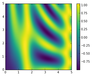
This section covers the use of Boolean masks to examine and manipulate values within NumPy arrays. Masking comes up when you want to extract, modify, count, or otherwise manipulate values in an array based on some criterion: for example, you might wish to count all values greater than a certain value, or perhaps remove all outliers that are above some threshold. In NumPy, Boolean masking is often the most efficient way to accomplish these types of tasks.
Imagine you have a series of data that represents the amount of precipitation each day for a year in a given city. For example, here we’ll load the daily rainfall statistics for the city of Seattle in 2014, using Pandas (which is covered in more detail in Chapter 3):
In[1]:importnumpyasnpimportpandasaspd# use Pandas to extract rainfall inches as a NumPy arrayrainfall=pd.read_csv('data/Seattle2014.csv')['PRCP'].valuesinches=rainfall/254# 1/10mm -> inchesinches.shape
Out[1]: (365,)
The array contains 365 values, giving daily rainfall in inches from January 1 to December 31, 2014.
As a first quick visualization, let’s look at the histogram of rainy days shown in Figure 2-6, which was generated using Matplotlib (we will explore this tool more fully in Chapter 4):
In[2]:%matplotlibinlineimportmatplotlib.pyplotaspltimportseaborn;seaborn.set()# set plot styles
In[3]:plt.hist(inches,40);
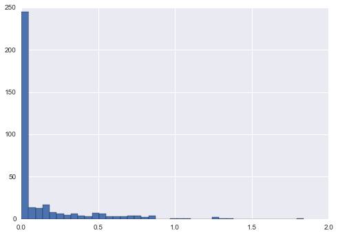
This histogram gives us a general idea of what the data looks like: despite its reputation, the vast majority of days in Seattle saw near zero measured rainfall in 2014. But this doesn’t do a good job of conveying some information we’d like to see: for example, how many rainy days were there in the year? What is the average precipitation on those rainy days? How many days were there with more than half an inch of rain?
One approach to this would be to answer these questions by hand: loop through the data, incrementing a counter each time we see values in some desired range. For reasons discussed throughout this chapter, such an approach is very inefficient, both from the standpoint of time writing code and time computing the result. We saw in “Computation on NumPy Arrays: Universal Functions” that NumPy’s ufuncs can be used in place of loops to do fast element-wise arithmetic operations on arrays; in the same way, we can use other ufuncs to do element-wise comparisons over arrays, and we can then manipulate the results to answer the questions we have. We’ll leave the data aside for right now, and discuss some general tools in NumPy to use masking to quickly answer these types of questions.
In “Computation on NumPy Arrays: Universal Functions” we introduced ufuncs, and focused in
particular on arithmetic operators. We saw that using +, -, *,
/, and others on arrays leads to element-wise operations. NumPy also
implements comparison operators such as < (less than) and > (greater
than) as element-wise ufuncs. The result of these comparison operators is
always an array with a Boolean data type. All six of the standard
comparison operations are available:
In[4]:x=np.array([1,2,3,4,5])
In[5]:x<3# less than
Out[5]: array([ True, True, False, False, False], dtype=bool)
In[6]:x>3# greater than
Out[6]: array([False, False, False, True, True], dtype=bool)
In[7]:x<=3# less than or equal
Out[7]: array([ True, True, True, False, False], dtype=bool)
In[8]:x>=3# greater than or equal
Out[8]: array([False, False, True, True, True], dtype=bool)
In[9]:x!=3# not equal
Out[9]: array([ True, True, False, True, True], dtype=bool)
In[10]:x==3# equal
Out[10]: array([False, False, True, False, False], dtype=bool)
It is also possible to do an element-by-element comparison of two arrays, and to include compound expressions:
In[11]:(2*x)==(x**2)
Out[11]: array([False, True, False, False, False], dtype=bool)
As in the case of arithmetic operators, the comparison operators are
implemented as ufuncs in NumPy; for example, when you write x < 3,
internally NumPy uses np.less(x, 3). A summary of the comparison
operators and their equivalent ufunc is shown here:
| Operator | Equivalent ufunc |
|---|---|
|
|
|
|
|
|
|
|
|
|
|
|
Just as in the case of arithmetic ufuncs, these will work on arrays of any size and shape. Here is a two-dimensional example:
In[12]:rng=np.random.RandomState(0)x=rng.randint(10,size=(3,4))x
Out[12]: array([[5, 0, 3, 3],
[7, 9, 3, 5],
[2, 4, 7, 6]])
In[13]:x<6
Out[13]: array([[ True, True, True, True],
[False, False, True, True],
[ True, True, False, False]], dtype=bool)
In each case, the result is a Boolean array, and NumPy provides a number of straightforward patterns for working with these Boolean results.
Given a Boolean array, there are a host of useful operations you can do.
We’ll work with x, the two-dimensional array we created earlier:
In[14]:(x)
[[5 0 3 3] [7 9 3 5] [2 4 7 6]]
To count the number of True entries in a Boolean array,
np.count_nonzero is useful:
In[15]:# how many values less than 6?np.count_nonzero(x<6)
Out[15]: 8
We see that there are eight array entries that are less than 6.
Another way to get at this information is to use np.sum; in this case,
False is interpreted as 0, and True is interpreted as 1:
In[16]:np.sum(x<6)
Out[16]: 8
The benefit of sum() is that like with other NumPy aggregation
functions, this summation can be done along rows or columns as well:
In[17]:# how many values less than 6 in each row?np.sum(x<6,axis=1)
Out[17]: array([4, 2, 2])
This counts the number of values less than 6 in each row of the matrix.
If we’re interested in quickly checking whether any or all the values
are true, we can use (you guessed it) np.any() or np.all():
In[18]:# are there any values greater than 8?np.any(x>8)
Out[18]: True
In[19]:# are there any values less than zero?np.any(x<0)
Out[19]: False
In[20]:# are all values less than 10?np.all(x<10)
Out[20]: True
In[21]:# are all values equal to 6?np.all(x==6)
Out[21]: False
np.all() and np.any() can be used along particular axes as well. For
example:
In[22]:# are all values in each row less than 8?np.all(x<8,axis=1)
Out[22]: array([ True, False, True], dtype=bool)
Here all the elements in the first and third rows are less than 8, while this is not the case for the second row.
Finally, a quick warning: as mentioned in
“Aggregations: Min, Max, and Everything in Between”, Python has built-in sum(), any(),
and all() functions. These have a different syntax than the NumPy
versions, and in particular will fail or produce unintended results when
used on multidimensional arrays. Be sure that you are using np.sum(),
np.any(), and np.all() for these examples!
We’ve already seen how we might count, say, all days with rain less than four
inches, or all days with rain greater than two inches. But what if we
want to know about all days with rain less than four inches and greater
than one inch? This is accomplished through Python’s bitwise logic
operators, &, |, ^, and ~. Like with the standard arithmetic
operators, NumPy overloads these as ufuncs that work element-wise on
(usually Boolean) arrays.
For example, we can address this sort of compound question as follows:
In[23]:np.sum((inches>0.5)&(inches<1))
Out[23]: 29
So we see that there are 29 days with rainfall between 0.5 and 1.0 inches.
Note that the parentheses here are important—because of operator precedence rules, with parentheses removed this expression would be evaluated as follows, which results in an error:
inches>(0.5&inches)<1
Using the equivalence of A AND B and NOT (A OR B) (which you may remember if you’ve taken an introductory logic course), we can compute the same result in a different manner:
In[24]:np.sum(~((inches<=0.5)|(inches>=1)))
Out[24]: 29
Combining comparison operators and Boolean operators on arrays can lead to a wide range of efficient logical operations.
The following table summarizes the bitwise Boolean operators and their equivalent ufuncs:
| Operator | Equivalent ufunc |
|---|---|
|
|
| |
|
|
|
|
|
Using these tools, we might start to answer the types of questions we have about our weather data. Here are some examples of results we can compute when combining masking with aggregations:
In[25]:("Number days without rain: ",np.sum(inches==0))("Number days with rain: ",np.sum(inches!=0))("Days with more than 0.5 inches:",np.sum(inches>0.5))("Rainy days with < 0.1 inches :",np.sum((inches>0)&(inches<0.2)))
Number days without rain: 215 Number days with rain: 150 Days with more than 0.5 inches: 37 Rainy days with < 0.1 inches : 75
In the preceding section, we looked at aggregates computed directly on Boolean arrays. A
more powerful pattern is to use Boolean arrays as masks, to select
particular subsets of the data themselves. Returning to our x array
from before, suppose we want an array of all values in the array that
are less than, say, 5:
In[26]:x
Out[26]: array([[5, 0, 3, 3],
[7, 9, 3, 5],
[2, 4, 7, 6]])
We can obtain a Boolean array for this condition easily, as we’ve already seen:
In[27]:x<5
Out[27]: array([[False, True, True, True],
[False, False, True, False],
[ True, True, False, False]], dtype=bool)
Now to select these values from the array, we can simply index on this Boolean array; this is known as a masking operation:
In[28]:x[x<5]
Out[28]: array([0, 3, 3, 3, 2, 4])
What is returned is a one-dimensional array filled with all the values
that meet this condition; in other words, all the values in positions
at which the mask array is True.
We are then free to operate on these values as we wish. For example, we can compute some relevant statistics on our Seattle rain data:
In[29]:# construct a mask of all rainy daysrainy=(inches>0)# construct a mask of all summer days (June 21st is the 172nd day)summer=(np.arange(365)-172<90)&(np.arange(365)-172>0)("Median precip on rainy days in 2014 (inches): ",np.median(inches[rainy]))("Median precip on summer days in 2014 (inches): ",np.median(inches[summer]))("Maximum precip on summer days in 2014 (inches): ",np.max(inches[summer]))("Median precip on non-summer rainy days (inches):",np.median(inches[rainy&~summer]))
Median precip on rainy days in 2014 (inches): 0.194881889764 Median precip on summer days in 2014 (inches): 0.0 Maximum precip on summer days in 2014 (inches): 0.850393700787 Median precip on non-summer rainy days (inches): 0.200787401575
By combining Boolean operations, masking operations, and aggregates, we can very quickly answer these sorts of questions for our dataset.
In the previous sections, we saw how to access and modify portions of
arrays using simple indices (e.g., arr[0]), slices (e.g., arr[:5]),
and Boolean masks (e.g., arr[arr > 0]). In this section, we’ll look at
another style of array indexing, known as fancy indexing. Fancy
indexing is like the simple indexing we’ve already seen, but we pass arrays of
indices in place of single scalars. This allows us to very quickly
access and modify complicated subsets of an array’s values.
Fancy indexing is conceptually simple: it means passing an array of indices to access multiple array elements at once. For example, consider the following array:
In[1]:importnumpyasnprand=np.random.RandomState(42)x=rand.randint(100,size=10)(x)
[51 92 14 71 60 20 82 86 74 74]
Suppose we want to access three different elements. We could do it like this:
In[2]:[x[3],x[7],x[2]]
Out[2]: [71, 86, 14]
Alternatively, we can pass a single list or array of indices to obtain the same result:
In[3]:ind=[3,7,4]x[ind]
Out[3]: array([71, 86, 60])
With fancy indexing, the shape of the result reflects the shape of the index arrays rather than the shape of the array being indexed:
In[4]:ind=np.array([[3,7],[4,5]])x[ind]
Out[4]: array([[71, 86],
[60, 20]])
Fancy indexing also works in multiple dimensions. Consider the following array:
In[5]:X=np.arange(12).reshape((3,4))X
Out[5]: array([[ 0, 1, 2, 3],
[ 4, 5, 6, 7],
[ 8, 9, 10, 11]])
Like with standard indexing, the first index refers to the row, and the second to the column:
In[6]:row=np.array([0,1,2])col=np.array([2,1,3])X[row,col]
Out[6]: array([ 2, 5, 11])
Notice that the first value in the result is X[0, 2], the second is
X[1, 1], and the third is X[2, 3]. The pairing of indices in fancy
indexing follows all the broadcasting rules that were mentioned in
“Computation on Arrays: Broadcasting”. So, for example, if we combine a column vector
and a row vector within the indices, we get a two-dimensional result:
In[7]:X[row[:,np.newaxis],col]
Out[7]: array([[ 2, 1, 3],
[ 6, 5, 7],
[10, 9, 11]])
Here, each row value is matched with each column vector, exactly as we saw in broadcasting of arithmetic operations. For example:
In[8]:row[:,np.newaxis]*col
Out[8]: array([[0, 0, 0],
[2, 1, 3],
[4, 2, 6]])
It is always important to remember with fancy indexing that the return value reflects the broadcasted shape of the indices, rather than the shape of the array being indexed.
For even more powerful operations, fancy indexing can be combined with the other indexing schemes we’ve seen:
In[9]:(X)
[[ 0 1 2 3] [ 4 5 6 7] [ 8 9 10 11]]
We can combine fancy and simple indices:
In[10]:X[2,[2,0,1]]
Out[10]: array([10, 8, 9])
We can also combine fancy indexing with slicing:
In[11]:X[1:,[2,0,1]]
Out[11]: array([[ 6, 4, 5],
[10, 8, 9]])
And we can combine fancy indexing with masking:
In[12]:mask=np.array([1,0,1,0],dtype=bool)X[row[:,np.newaxis],mask]
Out[12]: array([[ 0, 2],
[ 4, 6],
[ 8, 10]])
All of these indexing options combined lead to a very flexible set of operations for accessing and modifying array values.
One common use of fancy indexing is the selection of subsets of rows from a matrix. For example, we might have an N by D matrix representing N points in D dimensions, such as the following points drawn from a two-dimensional normal distribution:
In[13]:mean=[0,0]cov=[[1,2],[2,5]]X=rand.multivariate_normal(mean,cov,100)X.shape
Out[13]: (100, 2)
Using the plotting tools we will discuss in Chapter 4, we can visualize these points as a scatter plot (Figure 2-7):
In[14]:%matplotlibinlineimportmatplotlib.pyplotaspltimportseaborn;seaborn.set()# for plot stylingplt.scatter(X[:,0],X[:,1]);
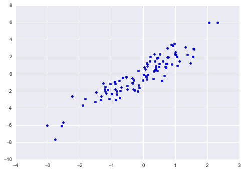
Let’s use fancy indexing to select 20 random points. We’ll do this by first choosing 20 random indices with no repeats, and use these indices to select a portion of the original array:
In[15]:indices=np.random.choice(X.shape[0],20,replace=False)indices
Out[15]: array([93, 45, 73, 81, 50, 10, 98, 94, 4, 64, 65, 89, 47, 84, 82,
80, 25, 90, 63, 20])
In[16]:selection=X[indices]# fancy indexing hereselection.shape
Out[16]: (20, 2)
Now to see which points were selected, let’s over-plot large circles at the locations of the selected points (Figure 2-8):
In[17]:plt.scatter(X[:,0],X[:,1],alpha=0.3)plt.scatter(selection[:,0],selection[:,1],facecolor='none',s=200);
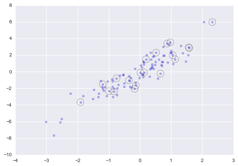
This sort of strategy is often used to quickly partition datasets, as is often needed in train/test splitting for validation of statistical models (see “Hyperparameters and Model Validation”), and in sampling approaches to answering statistical questions.
Just as fancy indexing can be used to access parts of an array, it can also be used to modify parts of an array. For example, imagine we have an array of indices and we’d like to set the corresponding items in an array to some value:
In[18]:x=np.arange(10)i=np.array([2,1,8,4])x[i]=99(x)
[ 0 99 99 3 99 5 6 7 99 9]
We can use any assignment-type operator for this. For example:
In[19]:x[i]-=10(x)
[ 0 89 89 3 89 5 6 7 89 9]
Notice, though, that repeated indices with these operations can cause some potentially unexpected results. Consider the following:
In[20]:x=np.zeros(10)x[[0,0]]=[4,6](x)
[ 6. 0. 0. 0. 0. 0. 0. 0. 0. 0.]
Where did the 4 go? The result of this operation is to first assign
x[0] = 4, followed by x[0] = 6. The result, of course, is that
x[0] contains the value 6.
Fair enough, but consider this operation:
In[21]:i=[2,3,3,4,4,4]x[i]+=1x
Out[21]: array([ 6., 0., 1., 1., 1., 0., 0., 0., 0., 0.])
You might expect that x[3] would contain the value 2, and x[4] would
contain the value 3, as this is how many times each index is repeated.
Why is this not the case? Conceptually, this is because x[i] += 1 is
meant as a shorthand of x[i] = x[i] + 1. x[i] + 1 is evaluated, and
then the result is assigned to the indices in x. With this in mind, it
is not the augmentation that happens multiple times, but the assignment,
which leads to the rather nonintuitive results.
So what if you want the other behavior where the operation is repeated?
For this, you can use the at() method of ufuncs (available since NumPy
1.8), and do the following:
In[22]:x=np.zeros(10)np.add.at(x,i,1)(x)
[ 0. 0. 1. 2. 3. 0. 0. 0. 0. 0.]
The at() method does an in-place application of the given operator at
the specified indices (here, i) with the specified value (here, 1).
Another method that is similar in spirit is the reduceat() method of
ufuncs, which you can read about in the NumPy documentation.
You can use these ideas to efficiently bin data to create a histogram
by hand. For example, imagine we have 1,000 values and would like to
quickly find where they fall within an array of bins. We could compute
it using ufunc.at like this:
In[23]:np.random.seed(42)x=np.random.randn(100)# compute a histogram by handbins=np.linspace(-5,5,20)counts=np.zeros_like(bins)# find the appropriate bin for each xi=np.searchsorted(bins,x)# add 1 to each of these binsnp.add.at(counts,i,1)
The counts now reflect the number of points within each bin—in other words, a histogram (Figure 2-9):
In[24]:# plot the resultsplt.plot(bins,counts,linestyle='steps');
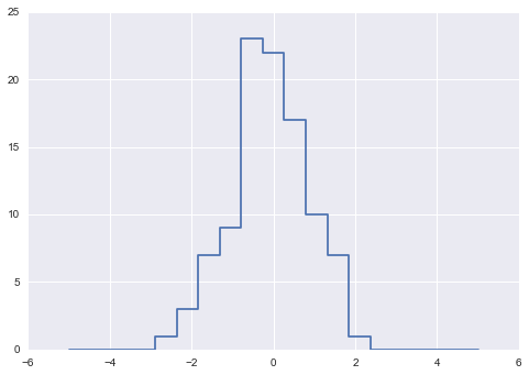
Of course, it would be silly to have to do this each time you want to
plot a histogram. This is why Matplotlib provides the plt.hist()
routine, which does the same in a single line:
plt.hist(x,bins,histtype='step');
This function will create a nearly identical plot to the one seen here.
To compute the binning, Matplotlib uses the np.histogram function,
which does a very similar computation to what we did before. Let’s
compare the two here:
In[25]:("NumPy routine:")%timeitcounts,edges=np.histogram(x,bins)("Custom routine:")%timeitnp.add.at(counts,np.searchsorted(bins,x),1)
NumPy routine: 10000 loops, best of 3: 97.6 µs per loop Custom routine: 10000 loops, best of 3: 19.5 µs per loop
Our own one-line algorithm is several times faster than the optimized
algorithm in NumPy! How can this be? If you dig into the np.histogram
source code (you can do this in IPython by typing np.histogram??),
you’ll see that it’s quite a bit more involved than the simple
search-and-count that we’ve done; this is because NumPy’s algorithm is
more flexible, and particularly is designed for better performance when
the number of data points becomes large:
In[26]:x=np.random.randn(1000000)("NumPy routine:")%timeitcounts,edges=np.histogram(x,bins)("Custom routine:")%timeitnp.add.at(counts,np.searchsorted(bins,x),1)
NumPy routine: 10 loops, best of 3: 68.7 ms per loop Custom routine: 10 loops, best of 3: 135 ms per loop
What this comparison shows is that algorithmic efficiency is almost
never a simple question. An algorithm efficient for large datasets will
not always be the best choice for small datasets, and vice versa (see
“Big-O Notation”). But the
advantage of coding this algorithm yourself is that with an
understanding of these basic methods, you could use these building
blocks to extend this to do some very interesting custom behaviors. The
key to efficiently using Python in data-intensive applications is
knowing about general convenience routines like np.histogram and when
they’re appropriate, but also knowing how to make use of lower-level
functionality when you need more pointed behavior.
Up to this point we have been concerned mainly with tools to access and operate on array data with NumPy. This section covers algorithms related to sorting values in NumPy arrays. These algorithms are a favorite topic in introductory computer science courses: if you’ve ever taken one, you probably have had dreams (or, depending on your temperament, nightmares) about insertion sorts, selection sorts, merge sorts, quick sorts, bubble sorts, and many, many more. All are means of accomplishing a similar task: sorting the values in a list or array.
For example, a simple selection sort repeatedly finds the minimum value from a list, and makes swaps until the list is sorted. We can code this in just a few lines of Python:
In[1]:importnumpyasnpdefselection_sort(x):foriinrange(len(x)):swap=i+np.argmin(x[i:])(x[i],x[swap])=(x[swap],x[i])returnx
In[2]:x=np.array([2,1,4,3,5])selection_sort(x)
Out[2]: array([1, 2, 3, 4, 5])
As any first-year computer science major will tell you, the selection
sort is useful for its simplicity, but is much too slow to be useful for
larger arrays. For a list of N values, it requires
N loops, each of which does on the order of ~ N
comparisons to find the swap value. In terms of the “big-O” notation
often used to characterize these algorithms (see “Big-O Notation”), selection sort averages  : if you double the number of items in the
list, the execution time will go up by about a factor of four.
: if you double the number of items in the
list, the execution time will go up by about a factor of four.
Even selection sort, though, is much better than my all-time favorite sorting algorithms, the bogosort:
In[3]:defbogosort(x):whilenp.any(x[:-1]>x[1:]):np.random.shuffle(x)returnx
In[4]:x=np.array([2,1,4,3,5])bogosort(x)
Out[4]: array([1, 2, 3, 4, 5])
This silly sorting method relies on pure chance: it repeatedly applies a
random shuffling of the array until the result happens to be sorted.
With an average scaling of  (that’s N times N factorial), this should—quite obviously—never
be used for any real computation.
(that’s N times N factorial), this should—quite obviously—never
be used for any real computation.
Fortunately, Python contains built-in sorting algorithms that are much more efficient than either of the simplistic algorithms just shown. We’ll start by looking at the Python built-ins, and then take a look at the routines included in NumPy and optimized for NumPy arrays.
Although Python has built-in sort and sorted functions to work
with lists, we won’t discuss them here because NumPy’s np.sort
function turns out to be much more efficient and useful for our
purposes. By default np.sort uses an  , quicksort algorithm, though
mergesort and heapsort are also available. For most applications,
the default quicksort is more than sufficient.
, quicksort algorithm, though
mergesort and heapsort are also available. For most applications,
the default quicksort is more than sufficient.
To return a sorted version of the array without modifying the input, you
can use np.sort:
In[5]:x=np.array([2,1,4,3,5])np.sort(x)
Out[5]: array([1, 2, 3, 4, 5])
If you prefer to sort the array in-place, you can instead use the sort
method of arrays:
In[6]:x.sort()(x)
[1 2 3 4 5]
A related function is argsort, which instead returns the indices of
the sorted elements:
In[7]:x=np.array([2,1,4,3,5])i=np.argsort(x)(i)
[1 0 3 2 4]
The first element of this result gives the index of the smallest element, the second value gives the index of the second smallest, and so on. These indices can then be used (via fancy indexing) to construct the sorted array if desired:
In[8]:x[i]
Out[8]: array([1, 2, 3, 4, 5])
A useful feature of NumPy’s sorting algorithms is the ability to sort
along specific rows or columns of a multidimensional array using the
axis argument. For example:
In[9]:rand=np.random.RandomState(42)X=rand.randint(0,10,(4,6))(X)
[[6 3 7 4 6 9] [2 6 7 4 3 7] [7 2 5 4 1 7] [5 1 4 0 9 5]]
In[10]:# sort each column of Xnp.sort(X,axis=0)
Out[10]: array([[2, 1, 4, 0, 1, 5],
[5, 2, 5, 4, 3, 7],
[6, 3, 7, 4, 6, 7],
[7, 6, 7, 4, 9, 9]])
In[11]:# sort each row of Xnp.sort(X,axis=1)
Out[11]: array([[3, 4, 6, 6, 7, 9],
[2, 3, 4, 6, 7, 7],
[1, 2, 4, 5, 7, 7],
[0, 1, 4, 5, 5, 9]])
Keep in mind that this treats each row or column as an independent array, and any relationships between the row or column values will be lost!
Sometimes we’re not interested in sorting the entire array, but simply want to find the K smallest values in the array. NumPy provides this
in the np.partition function. np.partition takes an array and a
number K; the result is a new array with the smallest K values to
the left of the partition, and the remaining values to the right, in
arbitrary order:
In[12]:x=np.array([7,2,3,1,6,5,4])np.partition(x,3)
Out[12]: array([2, 1, 3, 4, 6, 5, 7])
Note that the first three values in the resulting array are the three smallest in the array, and the remaining array positions contain the remaining values. Within the two partitions, the elements have arbitrary order.
Similarly to sorting, we can partition along an arbitrary axis of a multidimensional array:
In[13]:np.partition(X,2,axis=1)
Out[13]: array([[3, 4, 6, 7, 6, 9],
[2, 3, 4, 7, 6, 7],
[1, 2, 4, 5, 7, 7],
[0, 1, 4, 5, 9, 5]])
The result is an array where the first two slots in each row contain the smallest values from that row, with the remaining values filling the remaining slots.
Finally, just as there is a np.argsort that computes indices of the
sort, there is a np.argpartition that computes indices of the
partition. We’ll see this in action in the following section.
Let’s quickly see how we might use this argsort function along
multiple axes to find the nearest neighbors of each point in a set.
We’ll start by creating a random set of 10 points on a two-dimensional
plane. Using the standard convention, we’ll arrange these in a
10×2 array:
In[14]:X=rand.rand(10,2)
To get an idea of how these points look, let’s quickly scatter plot them (Figure 2-10):
In[15]:%matplotlibinlineimportmatplotlib.pyplotaspltimportseaborn;seaborn.set()# Plot stylingplt.scatter(X[:,0],X[:,1],s=100);
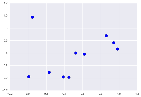
Now we’ll compute the distance between each pair of points. Recall that the squared-distance between two points is the sum of the squared differences in each dimension; using the efficient broadcasting (“Computation on Arrays: Broadcasting”) and aggregation (“Aggregations: Min, Max, and Everything in Between”) routines provided by NumPy, we can compute the matrix of square distances in a single line of code:
In[16]:dist_sq=np.sum((X[:,np.newaxis,:]-X[np.newaxis,:,:])**2,axis=-1)
This operation has a lot packed into it, and it might be a bit confusing if you’re unfamiliar with NumPy’s broadcasting rules. When you come across code like this, it can be useful to break it down into its component steps:
In[17]:# for each pair of points, compute differences in their coordinatesdifferences=X[:,np.newaxis,:]-X[np.newaxis,:,:]differences.shape
Out[17]: (10, 10, 2)
In[18]:# square the coordinate differencessq_differences=differences**2sq_differences.shape
Out[18]: (10, 10, 2)
In[19]:# sum the coordinate differences to get the squared distancedist_sq=sq_differences.sum(-1)dist_sq.shape
Out[19]: (10, 10)
Just to double-check what we are doing, we should see that the diagonal of this matrix (i.e., the set of distances between each point and itself) is all zero:
In[20]:dist_sq.diagonal()
Out[20]: array([ 0., 0., 0., 0., 0., 0., 0., 0., 0., 0.])
It checks out! With the pairwise square-distances converted, we can now
use np.argsort to sort along each row. The leftmost columns will then
give the indices of the nearest neighbors:
In[21]:nearest=np.argsort(dist_sq,axis=1)(nearest)
[[0 3 9 7 1 4 2 5 6 8] [1 4 7 9 3 6 8 5 0 2] [2 1 4 6 3 0 8 9 7 5] [3 9 7 0 1 4 5 8 6 2] [4 1 8 5 6 7 9 3 0 2] [5 8 6 4 1 7 9 3 2 0] [6 8 5 4 1 7 9 3 2 0] [7 9 3 1 4 0 5 8 6 2] [8 5 6 4 1 7 9 3 2 0] [9 7 3 0 1 4 5 8 6 2]]
Notice that the first column gives the numbers 0 through 9 in order: this is due to the fact that each point’s closest neighbor is itself, as we would expect.
By using a full sort here, we’ve actually done more work than we need to
in this case. If we’re simply interested in the nearest k
neighbors, all we need is to partition each row so that the smallest
k + 1 squared distances come first, with larger distances
filling the remaining positions of the array. We can do this with the
np.argpartition function:
In[22]:K=2nearest_partition=np.argpartition(dist_sq,K+1,axis=1)
In order to visualize this network of neighbors, let’s quickly plot the points along with lines representing the connections from each point to its two nearest neighbors (Figure 2-11):
In[23]:plt.scatter(X[:,0],X[:,1],s=100)# draw lines from each point to its two nearest neighborsK=2foriinrange(X.shape[0]):forjinnearest_partition[i,:K+1]:# plot a line from X[i] to X[j]# use some zip magic to make it happen:plt.plot(*zip(X[j],X[i]),color='black')
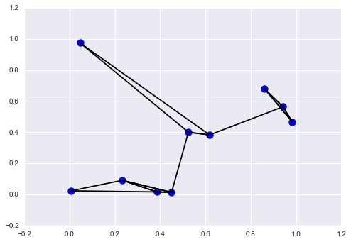
Each point in the plot has lines drawn to its two nearest neighbors. At first glance, it might seem strange that some of the points have more than two lines coming out of them: this is due to the fact that if point A is one of the two nearest neighbors of point B, this does not necessarily imply that point B is one of the two nearest neighbors of point A.
Although the broadcasting and row-wise sorting of this approach might seem less straightforward than writing a loop, it turns out to be a very efficient way of operating on this data in Python. You might be tempted to do the same type of operation by manually looping through the data and sorting each set of neighbors individually, but this would almost certainly lead to a slower algorithm than the vectorized version we used. The beauty of this approach is that it’s written in a way that’s agnostic to the size of the input data: we could just as easily compute the neighbors among 100 or 1,000,000 points in any number of dimensions, and the code would look the same.
Finally, I’ll note that when doing very large nearest-neighbor searches,
there are tree-based and/or approximate algorithms that can scale as
 or better rather than the
 of the brute-force algorithm. One
example of this is the KD-Tree,
implemented
in Scikit-Learn.
of the brute-force algorithm. One
example of this is the KD-Tree,
implemented
in Scikit-Learn.
While often our data can be well represented by a homogeneous array of
values, sometimes this is not the case. This section demonstrates the
use of NumPy’s structured arrays and record arrays, which provide
efficient storage for compound, heterogeneous data. While the patterns
shown here are useful for simple operations, scenarios like this often
lend themselves to the use of Pandas DataFrames, which we’ll explore in Chapter 3.
Imagine that we have several categories of data on a number of people (say, name, age, and weight), and we’d like to store these values for use in a Python program. It would be possible to store these in three separate arrays:
In[2]:name=['Alice','Bob','Cathy','Doug']age=[25,45,37,19]weight=[55.0,85.5,68.0,61.5]
But this is a bit clumsy. There’s nothing here that tells us that the three arrays are related; it would be more natural if we could use a single structure to store all of this data. NumPy can handle this through structured arrays, which are arrays with compound data types.
Recall that previously we created a simple array using an expression like this:
In[3]:x=np.zeros(4,dtype=int)
We can similarly create a structured array using a compound data type specification:
In[4]:# Use a compound data type for structured arraysdata=np.zeros(4,dtype={'names':('name','age','weight'),'formats':('U10','i4','f8')})(data.dtype)
[('name', '<U10'), ('age', '<i4'), ('weight', '<f8')]
Here 'U10' translates to “Unicode string of maximum length 10,” 'i4'
translates to “4-byte (i.e., 32 bit) integer,” and 'f8' translates to
“8-byte (i.e., 64 bit) float.” We’ll discuss other options for these type
codes in the following section.
Now that we’ve created an empty container array, we can fill the array with our lists of values:
In[5]:data['name']=namedata['age']=agedata['weight']=weight(data)
[('Alice', 25, 55.0) ('Bob', 45, 85.5) ('Cathy', 37, 68.0)
('Doug', 19, 61.5)]
As we had hoped, the data is now arranged together in one convenient block of memory.
The handy thing with structured arrays is that you can now refer to values either by index or by name:
In[6]:# Get all namesdata['name']
Out[6]: array(['Alice', 'Bob', 'Cathy', 'Doug'],
dtype='<U10')
In[7]:# Get first row of datadata[0]
Out[7]: ('Alice', 25, 55.0)
In[8]:# Get the name from the last rowdata[-1]['name']
Out[8]: 'Doug'
Using Boolean masking, this even allows you to do some more sophisticated operations such as filtering on age:
In[9]:# Get names where age is under 30data[data['age']<30]['name']
Out[9]: array(['Alice', 'Doug'],
dtype='<U10')
Note that if you’d like to do any operations that are any more
complicated than these, you should probably consider the Pandas package,
covered in the next chapter. As we’ll see, Pandas provides a DataFrame
object, which is a structure built on NumPy arrays that offers a variety
of useful data manipulation functionality similar to what we’ve shown
here, as well as much, much more.
Structured array data types can be specified in a number of ways. Earlier, we saw the dictionary method:
In[10]:np.dtype({'names':('name','age','weight'),'formats':('U10','i4','f8')})
Out[10]: dtype([('name', '<U10'), ('age', '<i4'), ('weight', '<f8')])
For clarity, numerical types can be specified with Python types or
NumPy dtypes instead:
In[11]:np.dtype({'names':('name','age','weight'),'formats':((np.str_,10),int,np.float32)})
Out[11]: dtype([('name', '<U10'), ('age', '<i8'), ('weight', '<f4')])
A compound type can also be specified as a list of tuples:
In[12]:np.dtype([('name','S10'),('age','i4'),('weight','f8')])
Out[12]: dtype([('name', 'S10'), ('age', '<i4'), ('weight', '<f8')])
If the names of the types do not matter to you, you can specify the types alone in a comma-separated string:
In[13]:np.dtype('S10,i4,f8')
Out[13]: dtype([('f0', 'S10'), ('f1', '<i4'), ('f2', '<f8')])
The shortened string format codes may seem confusing, but they are built
on simple principles. The first (optional) character is < or >,
which means “little endian” or “big endian,” respectively, and specifies
the ordering convention for significant bits. The next character
specifies the type of data: characters, bytes, ints, floating points,
and so on (see Table 2-4). The last character or characters represents
the size of the object in bytes.
| Character | Description | Example |
|---|---|---|
|
Byte |
|
|
Signed integer |
|
|
Unsigned integer |
|
|
Floating point |
|
|
Complex floating point |
|
|
string |
|
|
Unicode string |
|
|
Raw data (void) |
|
It is possible to define even more advanced compound types. For example,
you can create a type where each element contains an array or matrix of
values. Here, we’ll create a data type with a mat component consisting
of a 3×3 floating-point matrix:
In[14]:tp=np.dtype([('id','i8'),('mat','f8',(3,3))])X=np.zeros(1,dtype=tp)(X[0])(X['mat'][0])
(0, [[0.0, 0.0, 0.0], [0.0, 0.0, 0.0], [0.0, 0.0, 0.0]]) [[ 0. 0. 0.] [ 0. 0. 0.] [ 0. 0. 0.]]
Now each element in the X array consists of an id and a 3×3 matrix.
Why would you use this rather than a simple multidimensional array, or
perhaps a Python dictionary? The reason is that this NumPy dtype
directly maps onto a C structure definition, so the buffer containing
the array content can be accessed directly within an appropriately
written C program. If you find yourself writing a Python interface to a
legacy C or Fortran library that manipulates structured data, you’ll
probably find structured arrays quite useful!
NumPy also provides the np.recarray class, which is almost identical
to the structured arrays just described, but with one additional feature:
fields can be accessed as attributes rather than as dictionary keys.
Recall that we previously accessed the ages by writing:
In[15]:data['age']
Out[15]: array([25, 45, 37, 19], dtype=int32)
If we view our data as a record array instead, we can access this with slightly fewer keystrokes:
In[16]:data_rec=data.view(np.recarray)data_rec.age
Out[16]: array([25, 45, 37, 19], dtype=int32)
The downside is that for record arrays, there is some extra overhead involved in accessing the fields, even when using the same syntax. We can see this here:
In[17]:%timeitdata['age']%timeitdata_rec['age']%timeitdata_rec.age
1000000 loops, best of 3: 241 ns per loop 100000 loops, best of 3: 4.61 µs per loop 100000 loops, best of 3: 7.27 µs per loop
Whether the more convenient notation is worth the additional overhead will depend on your own application.
This section on structured and record arrays is purposely at the end of this chapter, because it leads so well into the next package we will cover: Pandas. Structured arrays like the ones discussed here are good to know about for certain situations, especially in case you’re using NumPy arrays to map onto binary data formats in C, Fortran, or another language. For day-to-day use of structured data, the Pandas package is a much better choice, and we’ll dive into a full discussion of it in the next chapter.
1 Code to produce this plot can be found in the online appendix, and is adapted from source published in the astroML documentation. Used with permission.
In the previous chapter, we dove into detail on NumPy and its ndarray
object, which provides efficient storage and manipulation of dense typed
arrays in Python. Here we’ll build on this knowledge by looking in
detail at the data structures provided by the Pandas library. Pandas is
a newer package built on top of NumPy, and provides an efficient
implementation of a DataFrame. DataFrames are essentially
multidimensional arrays with attached row and column labels, and often
with heterogeneous types and/or missing data. As well as offering a
convenient storage interface for labeled data, Pandas implements a
number of powerful data operations familiar to users of both database
frameworks and spreadsheet programs.
As we saw, NumPy’s ndarray data structure provides essential features
for the type of clean, well-organized data typically seen in numerical
computing tasks. While it serves this purpose very well, its limitations
become clear when we need more flexibility (attaching labels to
data, working with missing data, etc.) and when attempting operations
that do not map well to element-wise broadcasting (groupings,
pivots, etc.), each of which is an important piece of analyzing the less
structured data available in many forms in the world around us. Pandas,
and in particular its Series and DataFrame objects, builds on the
NumPy array structure and provides efficient access to these sorts of
“data munging” tasks that occupy much of a data scientist’s time.
In this chapter, we will focus on the mechanics of using Series, DataFrame, and related structures effectively. We will use
examples drawn from real datasets where appropriate, but these examples
are not necessarily the focus.
Installing Pandas on your system requires NumPy to be installed, and if you’re building the library from source, requires the appropriate tools to compile the C and Cython sources on which Pandas is built. Details on this installation can be found in the Pandas documentation. If you followed the advice outlined in the preface and used the Anaconda stack, you already have Pandas installed.
Once Pandas is installed, you can import it and check the version:
In[1]:importpandaspandas.__version__
Out[1]: '0.18.1'
Just as we generally import NumPy under the alias np, we will import Pandas under the alias pd:
In[2]:importpandasaspd
This import convention will be used throughout the remainder of this book.
At the very basic level, Pandas objects can be thought of as enhanced
versions of NumPy structured arrays in which the rows and columns are
identified with labels rather than simple integer indices. As we will
see during the course of this chapter, Pandas provides a host of useful
tools, methods, and functionality on top of the basic data structures, but
nearly everything that follows will require an understanding of what
these structures are. Thus, before we go any further, let’s introduce these three
fundamental Pandas data structures: the Series, DataFrame, and
Index.
We will start our code sessions with the standard NumPy and Pandas imports:
In[1]:importnumpyasnpimportpandasaspd
A Pandas Series is a one-dimensional array of indexed data. It can be
created from a list or array as follows:
In[2]:data=pd.Series([0.25,0.5,0.75,1.0])data
Out[2]: 0 0.25
1 0.50
2 0.75
3 1.00
dtype: float64
As we see in the preceding output, the Series wraps both a sequence of
values and a sequence of indices, which we can access with the values
and index attributes. The values are simply a familiar NumPy array:
In[3]:data.values
Out[3]: array([ 0.25, 0.5 , 0.75, 1. ])
The index is an array-like object of type pd.Index, which
we’ll discuss in more detail momentarily:
In[4]:data.index
Out[4]: RangeIndex(start=0, stop=4, step=1)
Like with a NumPy array, data can be accessed by the associated index via the familiar Python square-bracket notation:
In[5]:data[1]
Out[5]: 0.5
In[6]:data[1:3]
Out[6]: 1 0.50
2 0.75
dtype: float64
As we will see, though, the Pandas Series is much more general and
flexible than the one-dimensional NumPy array that it emulates.
From what we’ve seen so far, it may look like the Series object is
basically interchangeable with a one-dimensional NumPy array. The
essential difference is the presence of the index: while the NumPy array
has an implicitly defined integer index used to access the values, the
Pandas Series has an explicitly defined index associated with the
values.
This explicit index definition gives the Series object additional
capabilities. For example, the index need not be an integer, but can
consist of values of any desired type. For example, if we wish, we can
use strings as an index:
In[7]:data=pd.Series([0.25,0.5,0.75,1.0],index=['a','b','c','d'])data
Out[7]: a 0.25
b 0.50
c 0.75
d 1.00
dtype: float64
And the item access works as expected:
In[8]:data['b']
Out[8]: 0.5
We can even use noncontiguous or nonsequential indices:
In[9]:data=pd.Series([0.25,0.5,0.75,1.0],index=[2,5,3,7])data
Out[9]: 2 0.25
5 0.50
3 0.75
7 1.00
dtype: float64
In[10]:data[5]
Out[10]: 0.5
In this way, you can think of a Pandas Series a bit like a
specialization of a Python dictionary. A dictionary is a structure that
maps arbitrary keys to a set of arbitrary values, and a Series is a
structure that maps typed keys to a set of typed values. This
typing is important: just as the type-specific compiled code behind a
NumPy array makes it more efficient than a Python list for certain
operations, the type information of a Pandas Series makes it much more
efficient than Python dictionaries for certain operations.
We can make the Series-as-dictionary analogy even more clear by constructing a
Series object directly from a Python dictionary:
In[11]:population_dict={'California':38332521,'Texas':26448193,'New York':19651127,'Florida':19552860,'Illinois':12882135}population=pd.Series(population_dict)population
Out[11]: California 38332521
Florida 19552860
Illinois 12882135
New York 19651127
Texas 26448193
dtype: int64
By default, a Series will be created where the index is drawn from the
sorted keys. From here, typical dictionary-style item access can be
performed:
In[12]:population['California']
Out[12]: 38332521
Unlike a dictionary, though, the Series also supports array-style
operations such as slicing:
In[13]:population['California':'Illinois']
Out[13]: California 38332521
Florida 19552860
Illinois 12882135
dtype: int64
We’ll discuss some of the quirks of Pandas indexing and slicing in “Data Indexing and Selection”.
We’ve already seen a few ways of constructing a Pandas Series from
scratch; all of them are some version of the following:
>>>pd.Series(data,index=index)
where index is an optional argument, and data can be one of many
entities.
For example, data can be a list or NumPy array, in which case index
defaults to an integer sequence:
In[14]:pd.Series([2,4,6])
Out[14]: 0 2
1 4
2 6
dtype: int64
data can be a scalar, which is repeated to fill the specified index:
In[15]:pd.Series(5,index=[100,200,300])
Out[15]: 100 5
200 5
300 5
dtype: int64
data can be a dictionary, in which index defaults to the sorted
dictionary keys:
In[16]:pd.Series({2:'a',1:'b',3:'c'})
Out[16]: 1 b
2 a
3 c
dtype: object
In each case, the index can be explicitly set if a different result is preferred:
In[17]:pd.Series({2:'a',1:'b',3:'c'},index=[3,2])
Out[17]: 3 c
2 a
dtype: object
Notice that in this case, the Series is populated only with the
explicitly identified keys.
The next fundamental structure in Pandas is the DataFrame. Like the
Series object discussed in the previous section, the DataFrame can be thought of either as a
generalization of a NumPy array, or as a specialization of a Python
dictionary. We’ll now take a look at each of these perspectives.
If a Series is an analog of a one-dimensional array with flexible
indices, a DataFrame is an analog of a two-dimensional array with both
flexible row indices and flexible column names. Just as you might think
of a two-dimensional array as an ordered sequence of aligned
one-dimensional columns, you can think of a DataFrame as a sequence of
aligned Series objects. Here, by “aligned” we mean that they share the
same index.
To demonstrate this, let’s first construct a new Series listing the
area of each of the five states discussed in the previous section:
In[18]:area_dict={'California':423967,'Texas':695662,'New York':141297,'Florida':170312,'Illinois':149995}area=pd.Series(area_dict)area
Out[18]: California 423967
Florida 170312
Illinois 149995
New York 141297
Texas 695662
dtype: int64
Now that we have this along with the population Series from before, we
can use a dictionary to construct a single two-dimensional object
containing this information:
In[19]:states=pd.DataFrame({'population':population,'area':area})states
Out[19]: area population
California 423967 38332521
Florida 170312 19552860
Illinois 149995 12882135
New York 141297 19651127
Texas 695662 26448193
Like the Series object, the DataFrame has an index attribute that
gives access to the index labels:
In[20]:states.index
Out[20]: Index(['California', 'Florida', 'Illinois', 'New York', 'Texas'], dtype='object')
Additionally, the DataFrame has a columns attribute, which is an
Index object holding the column labels:
In[21]:states.columns
Out[21]: Index(['area', 'population'], dtype='object')
Thus the DataFrame can be thought of as a generalization of a
two-dimensional NumPy array, where both the rows and columns have a
generalized index for accessing the data.
Similarly, we can also think of a DataFrame as a specialization of a
dictionary. Where a dictionary maps a key to a value, a DataFrame maps
a column name to a Series of column data. For example, asking for the
'area' attribute returns the Series object containing the areas we
saw earlier:
In[22]:states['area']
Out[22]: California 423967
Florida 170312
Illinois 149995
New York 141297
Texas 695662
Name: area, dtype: int64
Notice the potential point of confusion here: in a two-dimensional NumPy
array, data[0] will return the first row. For a DataFrame,
data['col0'] will return the first column. Because of this, it is
probably better to think about DataFrames as generalized dictionaries
rather than generalized arrays, though both ways of looking at the
situation can be useful. We’ll explore more flexible means of indexing
DataFrames in “Data Indexing and Selection”.
A Pandas DataFrame can be constructed in a variety of ways. Here we’ll
give several examples.
A DataFrame is a collection of Series objects, and a single-column DataFrame can
be constructed from a single Series:
In[23]:pd.DataFrame(population,columns=['population'])
Out[23]: population
California 38332521
Florida 19552860
Illinois 12882135
New York 19651127
Texas 26448193
Any list of dictionaries can be made into a DataFrame. We’ll use a
simple list comprehension to create some data:
In[24]:data=[{'a':i,'b':2*i}foriinrange(3)]pd.DataFrame(data)
Out[24]: a b
0 0 0
1 1 2
2 2 4
Even if some keys in the dictionary are missing, Pandas will fill them
in with NaN (i.e., “not a number”) values:
In[25]:pd.DataFrame([{'a':1,'b':2},{'b':3,'c':4}])
Out[25]: a b c
0 1.0 2 NaN
1 NaN 3 4.0
As we saw before, a DataFrame can be constructed from a dictionary of
Series objects as well:
In[26]:pd.DataFrame({'population':population,'area':area})
Out[26]: area population
California 423967 38332521
Florida 170312 19552860
Illinois 149995 12882135
New York 141297 19651127
Texas 695662 26448193
Given a two-dimensional array of data, we can create a DataFrame with
any specified column and index names. If omitted, an integer index will
be used for each:
In[27]:pd.DataFrame(np.random.rand(3,2),columns=['foo','bar'],index=['a','b','c'])
Out[27]: foo bar
a 0.865257 0.213169
b 0.442759 0.108267
c 0.047110 0.905718
We covered structured arrays in
“Structured Data: NumPy’s Structured Arrays”. A Pandas DataFrame operates much like a structured
array, and can be created directly from one:
In[28]:A=np.zeros(3,dtype=[('A','i8'),('B','f8')])A
Out[28]: array([(0, 0.0), (0, 0.0), (0, 0.0)],
dtype=[('A', '<i8'), ('B', '<f8')])
In[29]:pd.DataFrame(A)
Out[29]: A B
0 0 0.0
1 0 0.0
2 0 0.0
We have seen here that both the Series and DataFrame objects contain an
explicit index that lets you reference and modify data. This Index
object is an interesting structure in itself, and it can be thought of
either as an immutable array or as an ordered set (technically a
multiset, as Index objects may contain repeated values). Those views
have some interesting consequences in the operations available on Index
objects. As a simple example, let’s construct an Index from a list of
integers:
In[30]:ind=pd.Index([2,3,5,7,11])ind
Out[30]: Int64Index([2, 3, 5, 7, 11], dtype='int64')
The Index object in many ways operates like an array. For example, we can use
standard Python indexing notation to retrieve values or slices:
In[31]:ind[1]
Out[31]: 3
In[32]:ind[::2]
Out[32]: Int64Index([2, 5, 11], dtype='int64')
Index objects also have many of the attributes familiar from NumPy
arrays:
In[33]:(ind.size,ind.shape,ind.ndim,ind.dtype)
5 (5,) 1 int64
One difference between Index objects and NumPy arrays is that indices
are immutable—that is, they cannot be modified via the normal means:
In[34]:ind[1]=0
---------------------------------------------------------------------------
TypeError Traceback (most recent call last)
<ipython-input-34-40e631c82e8a> in <module>()
----> 1 ind[1] = 0
/Users/jakevdp/anaconda/lib/python3.5/site-packages/pandas/indexes/base.py ...
1243
1244 def __setitem__(self, key, value):
-> 1245 raise TypeError("Index does not support mutable operations")
1246
1247 def __getitem__(self, key):
TypeError: Index does not support mutable operations
This immutability makes it safer to share indices between multiple
DataFrames and arrays, without the potential for side effects from
inadvertent index modification.
Pandas objects are designed to facilitate operations such as joins
across datasets, which depend on many aspects of set arithmetic. The
Index object follows many of the conventions used by Python’s built-in set
data structure, so that unions, intersections, differences, and other
combinations can be computed in a familiar way:
In[35]:indA=pd.Index([1,3,5,7,9])indB=pd.Index([2,3,5,7,11])
In[36]:indA&indB# intersection
Out[36]: Int64Index([3, 5, 7], dtype='int64')
In[37]:indA|indB# union
Out[37]: Int64Index([1, 2, 3, 5, 7, 9, 11], dtype='int64')
In[38]:indA^indB# symmetric difference
Out[38]: Int64Index([1, 2, 9, 11], dtype='int64')
These operations may also be accessed via object methods—for example, indA.intersection(indB).
In Chapter 2, we looked in detail at methods and tools to
access, set, and modify values in NumPy arrays. These included indexing
(e.g., arr[2, 1]), slicing (e.g., arr[:, 1:5]), masking (e.g.,
arr[arr > 0]), fancy indexing (e.g., arr[0, [1, 5]]), and
combinations thereof (e.g., arr[:, [1, 5]]). Here we’ll look at similar
means of accessing and modifying values in Pandas Series and
DataFrame objects. If you have used the NumPy patterns, the corresponding patterns in Pandas will feel very familiar,
though there are a few quirks to be aware of.
We’ll start with the simple case of the one-dimensional Series object,
and then move on to the more complicated two-dimensional DataFrame
object.
As we saw in the previous section, a Series object acts in many ways
like a one-dimensional NumPy array, and in many ways like a standard
Python dictionary. If we keep these two overlapping analogies in mind,
it will help us to understand the patterns of data indexing and
selection in these arrays.
Like a dictionary, the Series object provides a mapping from a
collection of keys to a collection of values:
In[1]:importpandasaspddata=pd.Series([0.25,0.5,0.75,1.0],index=['a','b','c','d'])data
Out[1]: a 0.25
b 0.50
c 0.75
d 1.00
dtype: float64
In[2]:data['b']
Out[2]: 0.5
We can also use dictionary-like Python expressions and methods to examine the keys/indices and values:
In[3]:'a'indata
Out[3]: True
In[4]:data.keys()
Out[4]: Index(['a', 'b', 'c', 'd'], dtype='object')
In[5]:list(data.items())
Out[5]: [('a', 0.25), ('b', 0.5), ('c', 0.75), ('d', 1.0)]
Series objects can even be modified with a dictionary-like syntax.
Just as you can extend a dictionary by assigning to a new key, you can
extend a Series by assigning to a new index value:
In[6]:data['e']=1.25data
Out[6]: a 0.25
b 0.50
c 0.75
d 1.00
e 1.25
dtype: float64
This easy mutability of the objects is a convenient feature: under the hood, Pandas is making decisions about memory layout and data copying that might need to take place; the user generally does not need to worry about these issues.
A Series builds on this dictionary-like interface and provides
array-style item selection via the same basic mechanisms as NumPy arrays—that is, slices, masking, and fancy indexing. Examples of these are
as follows:
In[7]:# slicing by explicit indexdata['a':'c']
Out[7]: a 0.25
b 0.50
c 0.75
dtype: float64
In[8]:# slicing by implicit integer indexdata[0:2]
Out[8]: a 0.25
b 0.50
dtype: float64
In[9]:# maskingdata[(data>0.3)&(data<0.8)]
Out[9]: b 0.50
c 0.75
dtype: float64
In[10]:# fancy indexingdata[['a','e']]
Out[10]: a 0.25
e 1.25
dtype: float64
Among these, slicing may be the source of the most confusion. Notice
that when you are slicing with an explicit index (i.e., data['a':'c']), the
final index is included in the slice, while when you’re slicing with an
implicit index (i.e., data[0:2]), the final index is excluded from
the slice.
These slicing and indexing conventions can be a source of confusion.
For example, if your Series has an explicit integer index, an indexing
operation such as data[1] will use the explicit indices, while a
slicing operation like data[1:3] will use the implicit Python-style
index.
In[11]:data=pd.Series(['a','b','c'],index=[1,3,5])data
Out[11]: 1 a
3 b
5 c
dtype: object
In[12]:# explicit index when indexingdata[1]
Out[12]: 'a'
In[13]:# implicit index when slicingdata[1:3]
Out[13]: 3 b
5 c
dtype: object
Because of this potential confusion in the case of integer indexes,
Pandas provides some special indexer attributes that explicitly
expose certain indexing schemes. These are not functional methods, but
attributes that expose a particular slicing interface to the data in
the Series.
First, the loc attribute allows indexing and slicing that always
references the explicit index:
In[14]:data.loc[1]
Out[14]: 'a'
In[15]:data.loc[1:3]
Out[15]: 1 a
3 b
dtype: object
The iloc attribute allows indexing and slicing that always references
the implicit Python-style index:
In[16]:data.iloc[1]
Out[16]: 'b'
In[17]:data.iloc[1:3]
Out[17]: 3 b
5 c
dtype: object
A third indexing attribute, ix, is a hybrid of the two, and for Series
objects is equivalent to standard []-based indexing. The purpose of
the ix indexer will become more apparent in the context of DataFrame
objects, which we will discuss in a moment.
One guiding principle of Python code is that “explicit is better than
implicit.” The explicit nature of loc and iloc make them very useful
in maintaining clean and readable code; especially in the case of
integer indexes, I recommend using these both to make code easier to
read and understand, and to prevent subtle bugs due to the mixed
indexing/slicing convention.
Recall that a DataFrame acts in many ways like a two-dimensional or
structured array, and in other ways like a dictionary of Series
structures sharing the same index. These analogies can be helpful to
keep in mind as we explore data selection within this structure.
The first analogy we will consider is the DataFrame as a dictionary of
related Series objects. Let’s return to our example of areas and
populations of states:
In[18]:area=pd.Series({'California':423967,'Texas':695662,'New York':141297,'Florida':170312,'Illinois':149995})pop=pd.Series({'California':38332521,'Texas':26448193,'New York':19651127,'Florida':19552860,'Illinois':12882135})data=pd.DataFrame({'area':area,'pop':pop})data
Out[18]: area pop
California 423967 38332521
Florida 170312 19552860
Illinois 149995 12882135
New York 141297 19651127
Texas 695662 26448193
The individual Series that make up the columns of the DataFrame can
be accessed via dictionary-style indexing of the column name:
In[19]:data['area']
Out[19]: California 423967
Florida 170312
Illinois 149995
New York 141297
Texas 695662
Name: area, dtype: int64
Equivalently, we can use attribute-style access with column names that are strings:
In[20]:data.area
Out[20]: California 423967
Florida 170312
Illinois 149995
New York 141297
Texas 695662
Name: area, dtype: int64
This attribute-style column access actually accesses the exact same object as the dictionary-style access:
In[21]:data.areaisdata['area']
Out[21]: True
Though this is a useful shorthand, keep in mind that it does not work
for all cases! For example, if the column names are not strings, or if
the column names conflict with methods of the DataFrame, this
attribute-style access is not possible. For example, the DataFrame has a
pop() method, so data.pop will point to this rather than the "pop"
column:
In[22]:data.popisdata['pop']
Out[22]: False
In particular, you should avoid the temptation to try column assignment
via attribute (i.e., use data['pop'] = z rather than data.pop = z).
Like with the Series objects discussed earlier, this dictionary-style syntax can
also be used to modify the object, in this case to add a new column:
In[23]:data['density']=data['pop']/data['area']data
Out[23]: area pop density
California 423967 38332521 90.413926
Florida 170312 19552860 114.806121
Illinois 149995 12882135 85.883763
New York 141297 19651127 139.076746
Texas 695662 26448193 38.018740
This shows a preview of the straightforward syntax of element-by-element
arithmetic between Series objects; we’ll dig into this further in
“Operating on Data in Pandas”.
As mentioned previously, we can also view the DataFrame as an enhanced
two-dimensional array. We can examine the raw underlying data array
using the values attribute:
In[24]:data.values
Out[24]: array([[ 4.23967000e+05, 3.83325210e+07, 9.04139261e+01],
[ 1.70312000e+05, 1.95528600e+07, 1.14806121e+02],
[ 1.49995000e+05, 1.28821350e+07, 8.58837628e+01],
[ 1.41297000e+05, 1.96511270e+07, 1.39076746e+02],
[ 6.95662000e+05, 2.64481930e+07, 3.80187404e+01]])
With this picture in mind, we can do many familiar array-like observations on the DataFrame itself. For example, we can transpose the full
DataFrame to swap rows and columns:
In[25]:data.T
Out[25]:
California Florida Illinois New York Texas
area 4.239670e+05 1.703120e+05 1.499950e+05 1.412970e+05 6.956620e+05
pop 3.833252e+07 1.955286e+07 1.288214e+07 1.965113e+07 2.644819e+07
density 9.041393e+01 1.148061e+02 8.588376e+01 1.390767e+02 3.801874e+01
When it comes to indexing of DataFrame objects, however, it is clear
that the dictionary-style indexing of columns precludes our ability to
simply treat it as a NumPy array. In particular, passing a single index
to an array accesses a row:
In[26]:data.values[0]
Out[26]: array([ 4.23967000e+05, 3.83325210e+07, 9.04139261e+01])
and passing a single “index” to a DataFrame accesses a column:
In[27]:data['area']
Out[27]: California 423967
Florida 170312
Illinois 149995
New York 141297
Texas 695662
Name: area, dtype: int64
Thus for array-style indexing, we need another convention. Here Pandas
again uses the loc, iloc, and ix indexers mentioned earlier. Using
the iloc indexer, we can index the underlying array as if it is a
simple NumPy array (using the implicit Python-style index), but the
DataFrame index and column labels are maintained in the result:
In[28]:data.iloc[:3,:2]
Out[28]: area pop
California 423967 38332521
Florida 170312 19552860
Illinois 149995 12882135
In[29]:data.loc[:'Illinois',:'pop']
Out[29]: area pop
California 423967 38332521
Florida 170312 19552860
Illinois 149995 12882135
The ix indexer allows a hybrid of these two approaches:
In[30]:data.ix[:3,:'pop']
Out[30]: area pop
California 423967 38332521
Florida 170312 19552860
Illinois 149995 12882135
Keep in mind that for integer indices, the ix indexer is subject to
the same potential sources of confusion as discussed for integer-indexed
Series objects.
Any of the familiar NumPy-style data access patterns can be used within
these indexers. For example, in the loc indexer we can combine masking
and fancy indexing as in the following:
In[31]:data.loc[data.density>100,['pop','density']]
Out[31]: pop density
Florida 19552860 114.806121
New York 19651127 139.076746
Any of these indexing conventions may also be used to set or modify values; this is done in the standard way that you might be accustomed to from working with NumPy:
In[32]:data.iloc[0,2]=90data
Out[32]: area pop density
California 423967 38332521 90.000000
Florida 170312 19552860 114.806121
Illinois 149995 12882135 85.883763
New York 141297 19651127 139.076746
Texas 695662 26448193 38.018740
To build up your fluency in Pandas data manipulation, I suggest spending
some time with a simple DataFrame and exploring the types of indexing,
slicing, masking, and fancy indexing that are allowed by these various
indexing approaches.
There are a couple extra indexing conventions that might seem at odds with the preceding discussion, but nevertheless can be very useful in practice. First, while indexing refers to columns, slicing refers to rows:
In[33]:data['Florida':'Illinois']
Out[33]: area pop density
Florida 170312 19552860 114.806121
Illinois 149995 12882135 85.883763
Such slices can also refer to rows by number rather than by index:
In[34]:data[1:3]
Out[34]: area pop density
Florida 170312 19552860 114.806121
Illinois 149995 12882135 85.883763
Similarly, direct masking operations are also interpreted row-wise rather than column-wise:
In[35]:data[data.density>100]
Out[35]: area pop density
Florida 170312 19552860 114.806121
New York 141297 19651127 139.076746
These two conventions are syntactically similar to those on a NumPy array, and while these may not precisely fit the mold of the Pandas conventions, they are nevertheless quite useful in practice.
One of the essential pieces of NumPy is the ability to perform quick element-wise operations, both with basic arithmetic (addition, subtraction, multiplication, etc.) and with more sophisticated operations (trigonometric functions, exponential and logarithmic functions, etc.). Pandas inherits much of this functionality from NumPy, and the ufuncs that we introduced in “Computation on NumPy Arrays: Universal Functions” are key to this.
Pandas includes a couple useful twists, however: for unary operations
like negation and trigonometric functions, these ufuncs will preserve
index and column labels in the output, and for binary operations such
as addition and multiplication, Pandas will automatically align
indices when passing the objects to the ufunc. This means that keeping
the context of data and combining data from different sources—both
potentially error-prone tasks with raw NumPy arrays—become essentially
foolproof ones with Pandas. We will additionally see that there are
well-defined operations between one-dimensional Series structures and
two-dimensional DataFrame structures.
Because Pandas is designed to work with NumPy, any NumPy ufunc will work
on Pandas Series and DataFrame objects. Let’s start by defining a simple
Series and DataFrame on which to demonstrate this:
In[1]:importpandasaspdimportnumpyasnp
In[2]:rng=np.random.RandomState(42)ser=pd.Series(rng.randint(0,10,4))ser
Out[2]: 0 6
1 3
2 7
3 4
dtype: int64
In[3]:df=pd.DataFrame(rng.randint(0,10,(3,4)),columns=['A','B','C','D'])df
Out[3]: A B C D
0 6 9 2 6
1 7 4 3 7
2 7 2 5 4
If we apply a NumPy ufunc on either of these objects, the result will be another Pandas object with the indices preserved:
In[4]:np.exp(ser)
Out[4]: 0 403.428793
1 20.085537
2 1096.633158
3 54.598150
dtype: float64
Or, for a slightly more complex calculation:
In[5]:np.sin(df*np.pi/4)
Out[5]: A B C D
0 -1.000000 7.071068e-01 1.000000 -1.000000e+00
1 -0.707107 1.224647e-16 0.707107 -7.071068e-01
2 -0.707107 1.000000e+00 -0.707107 1.224647e-16
Any of the ufuncs discussed in “Computation on NumPy Arrays: Universal Functions” can be used in a similar manner.
For binary operations on two Series or DataFrame objects, Pandas
will align indices in the process of performing the operation. This is
very convenient when you are working with incomplete data, as we’ll see in some
of the examples that follow.
As an example, suppose we are combining two different data sources, and find only the top three US states by area and the top three US states by population:
In[6]:area=pd.Series({'Alaska':1723337,'Texas':695662,'California':423967},name='area')population=pd.Series({'California':38332521,'Texas':26448193,'New York':19651127},name='population')
Let’s see what happens when we divide these to compute the population density:
In[7]:population/area
Out[7]: Alaska NaN
California 90.413926
New York NaN
Texas 38.018740
dtype: float64
The resulting array contains the union of indices of the two input arrays, which we could determine using standard Python set arithmetic on these indices:
In[8]:area.index|population.index
Out[8]: Index(['Alaska', 'California', 'New York', 'Texas'], dtype='object')
Any item for which one or the other does not have an entry is marked with
NaN, or “Not a Number,” which is how Pandas marks missing data (see
further discussion of missing data in
“Handling Missing Data”). This index
matching is implemented this way for any of Python’s built-in arithmetic
expressions; any missing values are filled in with NaN by default:
In[9]:A=pd.Series([2,4,6],index=[0,1,2])B=pd.Series([1,3,5],index=[1,2,3])A+B
Out[9]: 0 NaN
1 5.0
2 9.0
3 NaN
dtype: float64
If using NaN values is not the desired behavior, we can modify the fill value using appropriate object methods in place of the operators. For
example, calling A.add(B) is equivalent to calling A + B, but allows
optional explicit specification of the fill value for any elements in
A or B that might be missing:
In[10]:A.add(B,fill_value=0)
Out[10]: 0 2.0
1 5.0
2 9.0
3 5.0
dtype: float64
A similar type of alignment takes place for both columns and indices
when you are performing operations on DataFrames:
In[11]:A=pd.DataFrame(rng.randint(0,20,(2,2)),columns=list('AB'))A
Out[11]: A B
0 1 11
1 5 1
In[12]:B=pd.DataFrame(rng.randint(0,10,(3,3)),columns=list('BAC'))B
Out[12]: B A C
0 4 0 9
1 5 8 0
2 9 2 6
In[13]:A+B
Out[13]: A B C
0 1.0 15.0 NaN
1 13.0 6.0 NaN
2 NaN NaN NaN
Notice that indices are aligned correctly irrespective of their order in
the two objects, and indices in the result are sorted. As was the case with Series, we can use the associated object’s arithmetic method
and pass any desired fill_value to be used in place of missing
entries. Here we’ll fill with the mean of all values in A (which we compute by
first stacking the rows of A):
In[14]:fill=A.stack().mean()A.add(B,fill_value=fill)
Out[14]: A B C
0 1.0 15.0 13.5
1 13.0 6.0 4.5
2 6.5 13.5 10.5
Table 3-1 lists Python operators and their equivalent Pandas object methods.
| Python operator | Pandas method(s) |
|---|---|
|
|
|
|
|
|
|
|
|
|
|
|
|
|
When you are performing operations between a DataFrame and a Series, the
index and column alignment is similarly maintained. Operations between a
DataFrame and a Series are similar to operations between a two-dimensional and one-dimensional
NumPy array. Consider one common operation, where we find the difference
of a two-dimensional array and one of its rows:
In[15]:A=rng.randint(10,size=(3,4))A
Out[15]: array([[3, 8, 2, 4],
[2, 6, 4, 8],
[6, 1, 3, 8]])
In[16]:A-A[0]
Out[16]: array([[ 0, 0, 0, 0],
[-1, -2, 2, 4],
[ 3, -7, 1, 4]])
According to NumPy’s broadcasting rules (see “Computation on Arrays: Broadcasting”), subtraction between a two-dimensional array and one of its rows is applied row-wise.
In Pandas, the convention similarly operates row-wise by default:
In[17]:df=pd.DataFrame(A,columns=list('QRST'))df-df.iloc[0]
Out[17]: Q R S T
0 0 0 0 0
1 -1 -2 2 4
2 3 -7 1 4
If you would instead like to operate column-wise, you can use the object
methods mentioned earlier, while specifying the axis keyword:
In[18]:df.subtract(df['R'],axis=0)
Out[18]: Q R S T
0 -5 0 -6 -4
1 -4 0 -2 2
2 5 0 2 7
Note that these DataFrame/Series operations, like the operations
discussed before, will automatically align indices between the two
elements:
In[19]:halfrow=df.iloc[0,::2]halfrow
Out[19]: Q 3
S 2
Name: 0, dtype: int64
In[20]:df-halfrow
Out[20]: Q R S T
0 0.0 NaN 0.0 NaN
1 -1.0 NaN 2.0 NaN
2 3.0 NaN 1.0 NaN
This preservation and alignment of indices and columns means that operations on data in Pandas will always maintain the data context, which prevents the types of silly errors that might come up when you are working with heterogeneous and/or misaligned data in raw NumPy arrays.
The difference between data found in many tutorials and data in the real world is that real-world data is rarely clean and homogeneous. In particular, many interesting datasets will have some amount of data missing. To make matters even more complicated, different data sources may indicate missing data in different ways.
In this section, we will discuss some general considerations for missing data, discuss how Pandas chooses to represent it, and demonstrate some built-in Pandas tools for handling missing data in Python. Here and throughout the book, we’ll refer to missing data in general as null, NaN, or NA values.
A number of schemes have been developed to indicate the
presence of missing data in a table or DataFrame. Generally, they
revolve around one of two strategies: using a mask that globally
indicates missing values, or choosing a sentinel value that indicates
a missing entry.
In the masking approach, the mask might be an entirely separate Boolean array, or it may involve appropriation of one bit in the data representation to locally indicate the null status of a value.
In the sentinel approach, the sentinel value could be some data-specific convention, such as indicating a missing integer value with –9999 or some rare bit pattern, or it could be a more global convention, such as indicating a missing floating-point value with NaN (Not a Number), a special value which is part of the IEEE floating-point specification.
None of these approaches is without trade-offs: use of a separate mask array requires allocation of an additional Boolean array, which adds overhead in both storage and computation. A sentinel value reduces the range of valid values that can be represented, and may require extra (often non-optimized) logic in CPU and GPU arithmetic. Common special values like NaN are not available for all data types.
As in most cases where no universally optimal choice exists, different languages and systems use different conventions. For example, the R language uses reserved bit patterns within each data type as sentinel values indicating missing data, while the SciDB system uses an extra byte attached to every cell to indicate a NA state.
The way in which Pandas handles missing values is constrained by its reliance on the NumPy package, which does not have a built-in notion of NA values for non-floating-point data types.
Pandas could have followed R’s lead in specifying bit patterns for each individual data type to indicate nullness, but this approach turns out to be rather unwieldy. While R contains four basic data types, NumPy supports far more than this: for example, while R has a single integer type, NumPy supports fourteen basic integer types once you account for available precisions, signedness, and endianness of the encoding. Reserving a specific bit pattern in all available NumPy types would lead to an unwieldy amount of overhead in special-casing various operations for various types, likely even requiring a new fork of the NumPy package. Further, for the smaller data types (such as 8-bit integers), sacrificing a bit to use as a mask will significantly reduce the range of values it can represent.
NumPy does have support for masked arrays—that is, arrays that have a separate Boolean mask array attached for marking data as “good” or “bad.” Pandas could have derived from this, but the overhead in both storage, computation, and code maintenance makes that an unattractive choice.
With these constraints in mind, Pandas chose to use sentinels for
missing data, and further chose to use two already-existing Python null
values: the special floating-point NaN value, and the Python None
object. This choice has some side effects, as we will see, but in
practice ends up being a good compromise in most cases of interest.
The first sentinel value used by Pandas is None, a Python
singleton object that is often used for missing data in Python code.
Because None is a Python object, it cannot be used in any arbitrary
NumPy/Pandas array, but only in arrays with data type 'object' (i.e.,
arrays of Python objects):
In[1]:importnumpyasnpimportpandasaspd
In[2]:vals1=np.array([1,None,3,4])vals1
Out[2]: array([1, None, 3, 4], dtype=object)
This dtype=object means that the best common type representation NumPy
could infer for the contents of the array is that they are Python
objects. While this kind of object array is useful for some purposes,
any operations on the data will be done at the Python level, with much
more overhead than the typically fast operations seen for arrays with
native types:
In[3]:fordtypein['object','int']:("dtype =",dtype)%timeitnp.arange(1E6,dtype=dtype).sum()()
dtype = object 10 loops, best of 3: 78.2 ms per loop dtype = int 100 loops, best of 3: 3.06 ms per loop
The use of Python objects in an array also means that if you perform
aggregations like sum() or min() across an array with a None
value, you will generally get an error:
In[4]:vals1.sum()
TypeError Traceback (most recent call last)
<ipython-input-4-749fd8ae6030> in <module>()
----> 1 vals1.sum()
/Users/jakevdp/anaconda/lib/python3.5/site-packages/numpy/core/_methods.py ...
30
31 def _sum(a, axis=None, dtype=None, out=None, keepdims=False):
---> 32 return umr_sum(a, axis, dtype, out, keepdims)
33
34 def _prod(a, axis=None, dtype=None, out=None, keepdims=False):
TypeError: unsupported operand type(s) for +: 'int' and 'NoneType'
This reflects the fact that addition between an integer and None is
undefined.
The other missing data representation, NaN (acronym for Not a
Number), is different; it is a special floating-point value recognized by all systems that use the standard IEEE floating-point
representation:
In[5]:vals2=np.array([1,np.nan,3,4])vals2.dtype
Out[5]: dtype('float64')
Notice that NumPy chose a native floating-point type for this array:
this means that unlike the object array from before, this array supports fast
operations pushed into compiled code. You should be aware that NaN is
a bit like a data virus—it infects any other object it touches.
Regardless of the operation, the result of arithmetic with NaN will be
another NaN:
In[6]:1+np.nan
Out[6]: nan
In[7]:0*np.nan
Out[7]: nan
Note that this means that aggregates over the values are well defined (i.e., they don’t result in an error) but not always useful:
In[8]:vals2.sum(),vals2.min(),vals2.max()
Out[8]: (nan, nan, nan)
NumPy does provide some special aggregations that will ignore these missing values:
In[9]:np.nansum(vals2),np.nanmin(vals2),np.nanmax(vals2)
Out[9]: (8.0, 1.0, 4.0)
Keep in mind that NaN is specifically a floating-point value; there is
no equivalent NaN value for integers, strings, or other types.
NaN and None both have their place, and Pandas is built to handle
the two of them nearly interchangeably, converting between them where
appropriate:
In[10]:pd.Series([1,np.nan,2,None])
Out[10]: 0 1.0
1 NaN
2 2.0
3 NaN
dtype: float64
For types that don’t have an available sentinel value, Pandas
automatically type-casts when NA values are present. For example, if we
set a value in an integer array to np.nan, it will automatically be
upcast to a floating-point type to accommodate the NA:
In[11]:x=pd.Series(range(2),dtype=int)x
Out[11]: 0 0
1 1
dtype: int64
In[12]:x[0]=Nonex
Out[12]: 0 NaN
1 1.0
dtype: float64
Notice that in addition to casting the integer array to floating point,
Pandas automatically converts the None to a NaN value. (Be aware
that there is a proposal to add a native integer NA to Pandas in the
future; as of this writing, it has not been included.)
While this type of magic may feel a bit hackish compared to the more unified approach to NA values in domain-specific languages like R, the Pandas sentinel/casting approach works quite well in practice and in my experience only rarely causes issues.
Table 3-2 lists the upcasting conventions in Pandas when NA values are introduced.
| Typeclass | Conversion when storing NAs | NA sentinel value |
|---|---|---|
|
No change |
|
|
No change |
|
|
Cast to |
|
|
Cast to |
|
Keep in mind that in Pandas, string data is always stored with an
object dtype.
As we have seen, Pandas treats None and NaN as essentially
interchangeable for indicating missing or null values. To facilitate
this convention, there are several useful methods for detecting,
removing, and replacing null values in Pandas data structures. They are:
isnull()Generate a Boolean mask indicating missing values
notnull()Opposite of isnull()
dropna()Return a filtered version of the data
fillna()Return a copy of the data with missing values filled or imputed
We will conclude this section with a brief exploration and demonstration of these routines.
Pandas data structures have two useful methods for detecting null data:
isnull() and notnull(). Either one will return a Boolean mask over
the data. For example:
In[13]:data=pd.Series([1,np.nan,'hello',None])
In[14]:data.isnull()
Out[14]: 0 False
1 True
2 False
3 True
dtype: bool
As mentioned in “Data Indexing and Selection”, Boolean masks can be used directly as a Series
or DataFrame index:
In[15]:data[data.notnull()]
Out[15]: 0 1
2 hello
dtype: object
The isnull() and notnull() methods produce similar Boolean results
for DataFrames.
In addition to the masking used before, there are the convenience
methods, dropna() (which removes NA values) and fillna() (which fills in NA values). For a Series, the result is straightforward:
In[16]:data.dropna()
Out[16]: 0 1
2 hello
dtype: object
For a DataFrame, there are more options. Consider the following
DataFrame:
In[17]:df=pd.DataFrame([[1,np.nan,2],[2,3,5],[np.nan,4,6]])df
Out[17]: 0 1 2
0 1.0 NaN 2
1 2.0 3.0 5
2 NaN 4.0 6
We cannot drop single values from a DataFrame; we can only drop full
rows or full columns. Depending on the application, you might want one
or the other, so dropna() gives a number of options for a DataFrame.
By default, dropna() will drop all rows in which any null value is
present:
In[18]:df.dropna()
Out[18]: 0 1 2
1 2.0 3.0 5
Alternatively, you can drop NA values along a different axis; axis=1
drops all columns containing a null value:
In[19]:df.dropna(axis='columns')
Out[19]: 2
0 2
1 5
2 6
But this drops some good data as well; you might rather be interested in
dropping rows or columns with all NA values, or a majority of NA
values. This can be specified through the how or thresh parameters,
which allow fine control of the number of nulls to allow through.
The default is how='any', such that any row or column (depending on
the axis keyword) containing a null value will be dropped. You can
also specify how='all', which will only drop rows/columns that are
all null values:
In[20]:df[3]=np.nandf
Out[20]: 0 1 2 3
0 1.0 NaN 2 NaN
1 2.0 3.0 5 NaN
2 NaN 4.0 6 NaN
In[21]:df.dropna(axis='columns',how='all')
Out[21]: 0 1 2
0 1.0 NaN 2
1 2.0 3.0 5
2 NaN 4.0 6
For finer-grained control, the thresh parameter lets you specify a
minimum number of non-null values for the row/column to be kept:
In[22]:df.dropna(axis='rows',thresh=3)
Out[22]: 0 1 2 3
1 2.0 3.0 5 NaN
Here the first and last row have been dropped, because they contain only two non-null values.
Sometimes rather than dropping NA values, you’d rather replace them with
a valid value. This value might be a single number like zero, or it
might be some sort of imputation or interpolation from the good values.
You could do this in-place using the isnull() method as a mask, but
because it is such a common operation Pandas provides the fillna()
method, which returns a copy of the array with the null values replaced.
Consider the following Series:
In[23]:data=pd.Series([1,np.nan,2,None,3],index=list('abcde'))data
Out[23]: a 1.0
b NaN
c 2.0
d NaN
e 3.0
dtype: float64
We can fill NA entries with a single value, such as zero:
In[24]:data.fillna(0)
Out[24]: a 1.0
b 0.0
c 2.0
d 0.0
e 3.0
dtype: float64
We can specify a forward-fill to propagate the previous value forward:
In[25]:# forward-filldata.fillna(method='ffill')
Out[25]: a 1.0
b 1.0
c 2.0
d 2.0
e 3.0
dtype: float64
Or we can specify a back-fill to propagate the next values backward:
In[26]:# back-filldata.fillna(method='bfill')
Out[26]: a 1.0
b 2.0
c 2.0
d 3.0
e 3.0
dtype: float64
For DataFrames, the options are similar, but we can also specify an
axis along which the fills take place:
In[27]:df
Out[27]: 0 1 2 3
0 1.0 NaN 2 NaN
1 2.0 3.0 5 NaN
2 NaN 4.0 6 NaN
In[28]:df.fillna(method='ffill',axis=1)
Out[28]: 0 1 2 3
0 1.0 1.0 2.0 2.0
1 2.0 3.0 5.0 5.0
2 NaN 4.0 6.0 6.0
Notice that if a previous value is not available during a forward fill, the NA value remains.
Up to this point we’ve been focused primarily on one-dimensional and
two-dimensional data, stored in Pandas Series and DataFrame objects,
respectively. Often it is useful to go beyond this and store
higher-dimensional data—that is, data indexed by more than one or two
keys. While Pandas does provide Panel and Panel4D objects that
natively handle three-dimensional and four-dimensional data (see “Panel Data”), a far more common pattern in practice is to make use of
hierarchical indexing (also known as multi-indexing) to incorporate
multiple index levels within a single index. In this way,
higher-dimensional data can be compactly represented within the familiar
one-dimensional Series and two-dimensional DataFrame objects.
In this section, we’ll explore the direct creation of MultiIndex objects;
considerations around indexing, slicing, and computing statistics across
multiply indexed data; and useful routines for converting between simple
and hierarchically indexed representations of your data.
We begin with the standard imports:
In[1]:importpandasaspdimportnumpyasnp
Let’s start by considering how we might represent two-dimensional data
within a one-dimensional Series. For concreteness, we will consider a
series of data where each point has a character and numerical key.
Suppose you would like to track data about states from two different years. Using the Pandas tools we’ve already covered, you might be tempted to simply use Python tuples as keys:
In[2]:index=[('California',2000),('California',2010),('New York',2000),('New York',2010),('Texas',2000),('Texas',2010)]populations=[33871648,37253956,18976457,19378102,20851820,25145561]pop=pd.Series(populations,index=index)pop
Out[2]: (California, 2000) 33871648
(California, 2010) 37253956
(New York, 2000) 18976457
(New York, 2010) 19378102
(Texas, 2000) 20851820
(Texas, 2010) 25145561
dtype: int64
With this indexing scheme, you can straightforwardly index or slice the series based on this multiple index:
In[3]:pop[('California',2010):('Texas',2000)]
Out[3]: (California, 2010) 37253956
(New York, 2000) 18976457
(New York, 2010) 19378102
(Texas, 2000) 20851820
dtype: int64
But the convenience ends there. For example, if you need to select all values from 2010, you’ll need to do some messy (and potentially slow) munging to make it happen:
In[4]:pop[[iforiinpop.indexifi[1]==2010]]
Out[4]: (California, 2010) 37253956
(New York, 2010) 19378102
(Texas, 2010) 25145561
dtype: int64
This produces the desired result, but is not as clean (or as efficient for large datasets) as the slicing syntax we’ve grown to love in Pandas.
Fortunately, Pandas provides a better way. Our tuple-based indexing is
essentially a rudimentary multi-index, and the Pandas MultiIndex type
gives us the type of operations we wish to have. We can create a
multi-index from the tuples as follows:
In[5]:index=pd.MultiIndex.from_tuples(index)index
Out[5]: MultiIndex(levels=[['California', 'New York', 'Texas'], [2000, 2010]],
labels=[[0, 0, 1, 1, 2, 2], [0, 1, 0, 1, 0, 1]])
Notice that the MultiIndex contains multiple levels of indexing—in
this case, the state names and the years, as well as multiple labels
for each data point which encode these levels.
If we reindex our series with this MultiIndex, we see the hierarchical
representation of the data:
In[6]:pop=pop.reindex(index)pop
Out[6]: California 2000 33871648
2010 37253956
New York 2000 18976457
2010 19378102
Texas 2000 20851820
2010 25145561
dtype: int64
Here the first two columns of the Series representation show the
multiple index values, while the third column shows the data. Notice
that some entries are missing in the first column: in this multi-index
representation, any blank entry indicates the same value as the line
above it.
Now to access all data for which the second index is 2010, we can simply use the Pandas slicing notation:
In[7]:pop[:,2010]
Out[7]: California 37253956
New York 19378102
Texas 25145561
dtype: int64
The result is a singly indexed array with just the keys we’re interested in. This syntax is much more convenient (and the operation is much more efficient!) than the home-spun tuple-based multi-indexing solution that we started with. We’ll now further discuss this sort of indexing operation on hierarchically indexed data.
You might notice something else here: we could easily have stored the
same data using a simple DataFrame with index and column labels. In
fact, Pandas is built with this equivalence in mind. The unstack()
method will quickly convert a multiply-indexed Series into a
conventionally indexed DataFrame:
In[8]:pop_df=pop.unstack()pop_df
Out[8]: 2000 2010
California 33871648 37253956
New York 18976457 19378102
Texas 20851820 25145561
Naturally, the stack() method provides the opposite operation:
In[9]:pop_df.stack()
Out[9]: California 2000 33871648
2010 37253956
New York 2000 18976457
2010 19378102
Texas 2000 20851820
2010 25145561
dtype: int64
Seeing this, you might wonder why would we would bother with
hierarchical indexing at all. The reason is simple: just as we were able
to use multi-indexing to represent two-dimensional data within a
one-dimensional Series, we can also use it to represent data of three or more dimensions in a Series or DataFrame. Each extra level in a
multi-index represents an extra dimension of data; taking advantage of
this property gives us much more flexibility in the types of data we can
represent. Concretely, we might want to add another column of
demographic data for each state at each year (say, population under 18);
with a MultiIndex this is as easy as adding another column to the
DataFrame:
In[10]:pop_df=pd.DataFrame({'total':pop,'under18':[9267089,9284094,4687374,4318033,5906301,6879014]})pop_df
Out[10]: total under18
California 2000 33871648 9267089
2010 37253956 9284094
New York 2000 18976457 4687374
2010 19378102 4318033
Texas 2000 20851820 5906301
2010 25145561 6879014
In addition, all the ufuncs and other functionality discussed in “Operating on Data in Pandas” work with hierarchical indices as well. Here we compute the fraction of people under 18 by year, given the above data:
In[11]:f_u18=pop_df['under18']/pop_df['total']f_u18.unstack()
Out[11]: 2000 2010
California 0.273594 0.249211
New York 0.247010 0.222831
Texas 0.283251 0.273568
This allows us to easily and quickly manipulate and explore even high-dimensional data.
The most straightforward way to construct a multiply indexed Series or
DataFrame is to simply pass a list of two or more index arrays to the
constructor. For example:
In[12]:df=pd.DataFrame(np.random.rand(4,2),index=[['a','a','b','b'],[1,2,1,2]],columns=['data1','data2'])df
Out[12]: data1 data2
a 1 0.554233 0.356072
2 0.925244 0.219474
b 1 0.441759 0.610054
2 0.171495 0.886688
The work of creating the MultiIndex is done in the background.
Similarly, if you pass a dictionary with appropriate tuples as keys,
Pandas will automatically recognize this and use a MultiIndex by
default:
In[13]:data={('California',2000):33871648,('California',2010):37253956,('Texas',2000):20851820,('Texas',2010):25145561,('New York',2000):18976457,('New York',2010):19378102}pd.Series(data)
Out[13]: California 2000 33871648
2010 37253956
New York 2000 18976457
2010 19378102
Texas 2000 20851820
2010 25145561
dtype: int64
Nevertheless, it is sometimes useful to explicitly create a MultiIndex;
we’ll see a couple of these methods here.
For more flexibility in how the index is constructed, you can instead
use the class method constructors available in the pd.MultiIndex. For
example, as we did before, you can construct the MultiIndex from a
simple list of arrays, giving the index values within each level:
In[14]:pd.MultiIndex.from_arrays([['a','a','b','b'],[1,2,1,2]])
Out[14]: MultiIndex(levels=[['a', 'b'], [1, 2]],
labels=[[0, 0, 1, 1], [0, 1, 0, 1]])
You can construct it from a list of tuples, giving the multiple index values of each point:
In[15]:pd.MultiIndex.from_tuples([('a',1),('a',2),('b',1),('b',2)])
Out[15]: MultiIndex(levels=[['a', 'b'], [1, 2]],
labels=[[0, 0, 1, 1], [0, 1, 0, 1]])
You can even construct it from a Cartesian product of single indices:
In[16]:pd.MultiIndex.from_product([['a','b'],[1,2]])
Out[16]: MultiIndex(levels=[['a', 'b'], [1, 2]],
labels=[[0, 0, 1, 1], [0, 1, 0, 1]])
Similarly, you can construct the MultiIndex directly using its internal
encoding by passing levels (a list of lists containing available index
values for each level) and labels (a list of lists that reference
these labels):
In[17]:pd.MultiIndex(levels=[['a','b'],[1,2]],labels=[[0,0,1,1],[0,1,0,1]])
Out[17]: MultiIndex(levels=[['a', 'b'], [1, 2]],
labels=[[0, 0, 1, 1], [0, 1, 0, 1]])
You can pass any of these objects as the index argument when creating
a Series or DataFrame, or to the reindex method of an
existing Series or DataFrame.
Sometimes it is convenient to name the levels of the MultiIndex. You can accomplish this by passing the names argument to any of the above
MultiIndex constructors, or by setting the names attribute of the
index after the fact:
In[18]:pop.index.names=['state','year']pop
Out[18]: state year
California 2000 33871648
2010 37253956
New York 2000 18976457
2010 19378102
Texas 2000 20851820
2010 25145561
dtype: int64
With more involved datasets, this can be a useful way to keep track of the meaning of various index values.
In a DataFrame, the rows and columns are completely symmetric, and just
as the rows can have multiple levels of indices, the columns can have
multiple levels as well. Consider the following, which is a mock-up of
some (somewhat realistic) medical data:
In[19]:# hierarchical indices and columnsindex=pd.MultiIndex.from_product([[2013,2014],[1,2]],names=['year','visit'])columns=pd.MultiIndex.from_product([['Bob','Guido','Sue'],['HR','Temp']],names=['subject','type'])# mock some datadata=np.round(np.random.randn(4,6),1)data[:,::2]*=10data+=37# create the DataFramehealth_data=pd.DataFrame(data,index=index,columns=columns)health_data
Out[19]: subject Bob Guido Sue
type HR Temp HR Temp HR Temp
year visit
2013 1 31.0 38.7 32.0 36.7 35.0 37.2
2 44.0 37.7 50.0 35.0 29.0 36.7
2014 1 30.0 37.4 39.0 37.8 61.0 36.9
2 47.0 37.8 48.0 37.3 51.0 36.5
Here we see where the multi-indexing for both rows and columns can come
in very handy. This is fundamentally four-dimensional data, where the
dimensions are the subject, the measurement type, the year, and the
visit number. With this in place we can, for example, index the top-level column by the person’s name and get a full DataFrame containing
just that person’s information:
In[20]:health_data['Guido']
Out[20]: type HR Temp
year visit
2013 1 32.0 36.7
2 50.0 35.0
2014 1 39.0 37.8
2 48.0 37.3
For complicated records containing multiple labeled measurements across multiple times for many subjects (people, countries, cities, etc.), use of hierarchical rows and columns can be extremely convenient!
Indexing and slicing on a MultiIndex is designed to be intuitive, and it
helps if you think about the indices as added dimensions. We’ll first
look at indexing multiply indexed Series, and then multiply indexed
DataFrames.
Consider the multiply indexed Series of state populations we saw earlier:
In[21]:pop
Out[21]: state year
California 2000 33871648
2010 37253956
New York 2000 18976457
2010 19378102
Texas 2000 20851820
2010 25145561
dtype: int64
We can access single elements by indexing with multiple terms:
In[22]:pop['California',2000]
Out[22]: 33871648
The MultiIndex also supports partial indexing, or indexing just one of
the levels in the index. The result is another Series, with the
lower-level indices maintained:
In[23]:pop['California']
Out[23]: year
2000 33871648
2010 37253956
dtype: int64
Partial slicing is available as well, as long as the MultiIndex is
sorted (see discussion in “Sorted and unsorted indices”):
In[24]:pop.loc['California':'New York']
Out[24]: state year
California 2000 33871648
2010 37253956
New York 2000 18976457
2010 19378102
dtype: int64
With sorted indices, we can perform partial indexing on lower levels by passing an empty slice in the first index:
In[25]:pop[:,2000]
Out[25]: state
California 33871648
New York 18976457
Texas 20851820
dtype: int64
Other types of indexing and selection (discussed in “Data Indexing and Selection”) work as well; for example, selection based on Boolean masks:
In[26]:pop[pop>22000000]
Out[26]: state year
California 2000 33871648
2010 37253956
Texas 2010 25145561
dtype: int64
Selection based on fancy indexing also works:
In[27]:pop[['California','Texas']]
Out[27]: state year
California 2000 33871648
2010 37253956
Texas 2000 20851820
2010 25145561
dtype: int64
A multiply indexed DataFrame behaves in a similar manner. Consider our
toy medical DataFrame from before:
In[28]:health_data
Out[28]: subject Bob Guido Sue
type HR Temp HR Temp HR Temp
year visit
2013 1 31.0 38.7 32.0 36.7 35.0 37.2
2 44.0 37.7 50.0 35.0 29.0 36.7
2014 1 30.0 37.4 39.0 37.8 61.0 36.9
2 47.0 37.8 48.0 37.3 51.0 36.5
Remember that columns are primary in a DataFrame, and the syntax used
for multiply indexed Series applies to the columns. For example,
we can recover Guido’s heart rate data with a simple operation:
In[29]:health_data['Guido','HR']
Out[29]: year visit
2013 1 32.0
2 50.0
2014 1 39.0
2 48.0
Name: (Guido, HR), dtype: float64
Also, as with the single-index case, we can use the loc, iloc,
and ix indexers introduced in
“Data Indexing and Selection”. For example:
In[30]:health_data.iloc[:2,:2]
Out[30]: subject Bob
type HR Temp
year visit
2013 1 31.0 38.7
2 44.0 37.7
These indexers provide an array-like view of the underlying
two-dimensional data, but each individual index in loc or iloc can
be passed a tuple of multiple indices. For example:
In[31]:health_data.loc[:,('Bob','HR')]
Out[31]: year visit
2013 1 31.0
2 44.0
2014 1 30.0
2 47.0
Name: (Bob, HR), dtype: float64
Working with slices within these index tuples is not especially convenient; trying to create a slice within a tuple will lead to a syntax error:
In[32]:health_data.loc[(:,1),(:,'HR')]
File "<ipython-input-32-8e3cc151e316>", line 1
health_data.loc[(:, 1), (:, 'HR')]
^
SyntaxError: invalid syntax
You could get around this by building the desired slice explicitly using
Python’s built-in slice() function, but a better way in this context
is to use an IndexSlice object, which Pandas provides for precisely
this situation. For example:
In[33]:idx=pd.IndexSlicehealth_data.loc[idx[:,1],idx[:,'HR']]
Out[33]: subject Bob Guido Sue
type HR HR HR
year visit
2013 1 31.0 32.0 35.0
2014 1 30.0 39.0 61.0
There are so many ways to interact with data in multiply indexed Series
and DataFrames, and as with many tools in this book the best way to
become familiar with them is to try them out!
One of the keys to working with multiply indexed data is knowing how to
effectively transform the data. There are a number of operations that
will preserve all the information in the dataset, but rearrange it for
the purposes of various computations. We saw a brief example of this in
the stack() and unstack() methods, but there are many more
ways to finely control the rearrangement of data between hierarchical
indices and columns, and we’ll explore them here.
Earlier, we briefly mentioned a caveat, but we should emphasize it more
here. Many of the MultiIndex slicing operations will fail if the index
is not sorted. Let’s take a look at this here.
We’ll start by creating some simple multiply indexed data where the indices are not lexographically sorted:
In[34]:index=pd.MultiIndex.from_product([['a','c','b'],[1,2]])data=pd.Series(np.random.rand(6),index=index)data.index.names=['char','int']data
Out[34]: char int
a 1 0.003001
2 0.164974
c 1 0.741650
2 0.569264
b 1 0.001693
2 0.526226
dtype: float64
If we try to take a partial slice of this index, it will result in an error:
In[35]:try:data['a':'b']exceptKeyErrorase:(type(e))(e)
<class 'KeyError'> 'Key length (1) was greater than MultiIndex lexsort depth (0)'
Although it is not entirely clear from the error message, this is the
result of the MultiIndex not being sorted. For various
reasons, partial slices and other similar operations require the levels
in the MultiIndex to be in sorted (i.e., lexographical) order. Pandas
provides a number of convenience routines to perform this type of
sorting; examples are the sort_index() and sortlevel() methods of
the DataFrame. We’ll use the simplest, sort_index(), here:
In[36]:data=data.sort_index()data
Out[36]: char int
a 1 0.003001
2 0.164974
b 1 0.001693
2 0.526226
c 1 0.741650
2 0.569264
dtype: float64
With the index sorted in this way, partial slicing will work as expected:
In[37]:data['a':'b']
Out[37]: char int
a 1 0.003001
2 0.164974
b 1 0.001693
2 0.526226
dtype: float64
As we saw briefly before, it is possible to convert a dataset from a stacked multi-index to a simple two-dimensional representation, optionally specifying the level to use:
In[38]:pop.unstack(level=0)
Out[38]: state California New York Texas
year
2000 33871648 18976457 20851820
2010 37253956 19378102 25145561
In[39]:pop.unstack(level=1)
Out[39]: year 2000 2010
state
California 33871648 37253956
New York 18976457 19378102
Texas 20851820 25145561
The opposite of unstack() is stack(), which here can be used to
recover the original series:
In[40]:pop.unstack().stack()
Out[40]: state year
California 2000 33871648
2010 37253956
New York 2000 18976457
2010 19378102
Texas 2000 20851820
2010 25145561
dtype: int64
Another way to rearrange hierarchical data is to turn the index labels
into columns; this can be accomplished with the reset_index method.
Calling this on the population dictionary will result in a DataFrame
with a state and year column holding the information that was
formerly in the index. For clarity, we can optionally specify the name
of the data for the column representation:
In[41]:pop_flat=pop.reset_index(name='population')pop_flat
Out[41]: state year population
0 California 2000 33871648
1 California 2010 37253956
2 New York 2000 18976457
3 New York 2010 19378102
4 Texas 2000 20851820
5 Texas 2010 25145561
Often when you are working with data in the real world, the raw input data looks
like this and it’s useful to build a MultiIndex from the column values.
This can be done with the set_index method of the DataFrame, which
returns a multiply indexed DataFrame:
In[42]:pop_flat.set_index(['state','year'])
Out[42]: population
state year
California 2000 33871648
2010 37253956
New York 2000 18976457
2010 19378102
Texas 2000 20851820
2010 25145561
In practice, I find this type of reindexing to be one of the more useful patterns when I encounter real-world datasets.
We’ve previously seen that Pandas has built-in data aggregation methods,
such as mean(), sum(), and max(). For hierarchically indexed
data, these can be passed a level parameter that controls which
subset of the data the aggregate is computed on.
For example, let’s return to our health data:
In[43]:health_data
Out[43]: subject Bob Guido Sue
type HR Temp HR Temp HR Temp
year visit
2013 1 31.0 38.7 32.0 36.7 35.0 37.2
2 44.0 37.7 50.0 35.0 29.0 36.7
2014 1 30.0 37.4 39.0 37.8 61.0 36.9
2 47.0 37.8 48.0 37.3 51.0 36.5
Perhaps we’d like to average out the measurements in the two visits each year. We can do this by naming the index level we’d like to explore, in this case the year:
In[44]:data_mean=health_data.mean(level='year')data_mean
Out[44]: subject Bob Guido Sue
type HR Temp HR Temp HR Temp
year
2013 37.5 38.2 41.0 35.85 32.0 36.95
2014 38.5 37.6 43.5 37.55 56.0 36.70
By further making use of the axis keyword, we can take the mean among
levels on the columns as well:
In[45]:data_mean.mean(axis=1,level='type')
Out[45]: type HR Temp
year
2013 36.833333 37.000000
2014 46.000000 37.283333
Thus in two lines, we’ve been able to find the average heart rate and
temperature measured among all subjects in all visits each year. This
syntax is actually a shortcut to the GroupBy functionality, which we
will discuss in “Aggregation and Grouping”. While this is a toy example, many real-world datasets
have similar hierarchical structure.
Some of the most interesting studies of data come from combining
different data sources. These operations can involve anything from very
straightforward concatenation of two different datasets, to more
complicated database-style joins and merges that correctly handle any
overlaps between the datasets. Series and DataFrames are built
with this type of operation in mind, and Pandas includes functions and
methods that make this sort of data wrangling fast and straightforward.
Here we’ll take a look at simple concatenation of Series and DataFrames
with the pd.concat function; later we’ll dive into more sophisticated
in-memory merges and joins implemented in Pandas.
We begin with the standard imports:
In[1]:importpandasaspdimportnumpyasnp
For convenience, we’ll define this function, which creates a DataFrame of
a particular form that will be useful below:
In[2]:defmake_df(cols,ind):"""Quickly make a DataFrame"""data={c:[str(c)+str(i)foriinind]forcincols}returnpd.DataFrame(data,ind)# example DataFramemake_df('ABC',range(3))
Out[2]: A B C
0 A0 B0 C0
1 A1 B1 C1
2 A2 B2 C2
Concatenation of Series and DataFrame objects is very similar to concatenation
of NumPy arrays, which can be done via the np.concatenate function as
discussed in “The Basics of NumPy Arrays”. Recall that with it, you can combine the contents of two
or more arrays into a single array:
In[4]:x=[1,2,3]y=[4,5,6]z=[7,8,9]np.concatenate([x,y,z])
Out[4]: array([1, 2, 3, 4, 5, 6, 7, 8, 9])
The first argument is a list or tuple of arrays to concatenate.
Additionally, it takes an axis keyword that allows you to specify the
axis along which the result will be concatenated:
In[5]:x=[[1,2],[3,4]]np.concatenate([x,x],axis=1)
Out[5]: array([[1, 2, 1, 2],
[3, 4, 3, 4]])
Pandas has a function, pd.concat(), which has a similar
syntax to np.concatenate but contains a number of options that we’ll discuss momentarily:
# Signature in Pandas v0.18pd.concat(objs,axis=0,join='outer',join_axes=None,ignore_index=False,keys=None,levels=None,names=None,verify_integrity=False,copy=True)
pd.concat() can be used for a simple concatenation of Series or
DataFrame objects, just as np.concatenate() can be used for simple
concatenations of arrays:
In[6]:ser1=pd.Series(['A','B','C'],index=[1,2,3])ser2=pd.Series(['D','E','F'],index=[4,5,6])pd.concat([ser1,ser2])
Out[6]: 1 A
2 B
3 C
4 D
5 E
6 F
dtype: object
It also works to concatenate higher-dimensional objects, such as
DataFrames:
In[7]:df1=make_df('AB',[1,2])df2=make_df('AB',[3,4])(df1);(df2);(pd.concat([df1,df2]))
df1 df2 pd.concat([df1, df2])
A B A B A B
1 A1 B1 3 A3 B3 1 A1 B1
2 A2 B2 4 A4 B4 2 A2 B2
3 A3 B3
4 A4 B4
By default, the concatenation takes place row-wise within the DataFrame
(i.e., axis=0). Like np.concatenate, pd.concat allows specification
of an axis along which concatenation will take place. Consider the
following example:
In[8]:df3=make_df('AB',[0,1])df4=make_df('CD',[0,1])(df3);(df4);(pd.concat([df3,df4],axis='col'))
df3 df4 pd.concat([df3, df4], axis='col')
A B C D A B C D
0 A0 B0 0 C0 D0 0 A0 B0 C0 D0
1 A1 B1 1 C1 D1 1 A1 B1 C1 D1
We could have equivalently specified axis=1; here we’ve used the more
intuitive axis='col'.
One important difference between np.concatenate and pd.concat is
that Pandas concatenation preserves indices, even if the result will
have duplicate indices! Consider this simple example:
In[9]:x=make_df('AB',[0,1])y=make_df('AB',[2,3])y.index=x.index# make duplicate indices!(x);(y);(pd.concat([x,y]))
x y pd.concat([x, y])
A B A B A B
0 A0 B0 0 A2 B2 0 A0 B0
1 A1 B1 1 A3 B3 1 A1 B1
0 A2 B2
1 A3 B3
Notice the repeated indices in the result. While this is valid within
DataFrames, the outcome is often undesirable. pd.concat() gives us a
few ways to handle it.
If you’d like to simply verify that the indices in the result of
pd.concat() do not overlap, you can specify the verify_integrity
flag. With this set to True, the concatenation will raise an exception
if there are duplicate indices. Here is an example, where for clarity
we’ll catch and print the error message:
In[10]:try:pd.concat([x,y],verify_integrity=True)exceptValueErrorase:("ValueError:",e)
ValueError: Indexes have overlapping values: [0, 1]
Sometimes the index itself does not matter, and you would prefer it to
simply be ignored. You can specify this option using the ignore_index
flag. With this set to True, the concatenation will create a new integer
index for the resulting Series:
In[11]:(x);(y);(pd.concat([x,y],ignore_index=True))
x y pd.concat([x, y], ignore_index=True)
A B A B A B
0 A0 B0 0 A2 B2 0 A0 B0
1 A1 B1 1 A3 B3 1 A1 B1
2 A2 B2
3 A3 B3
Another alternative is to use the keys option to specify a label for the
data sources; the result will be a hierarchically indexed series
containing the data:
In[12]:(x);(y);(pd.concat([x,y],keys=['x','y']))
x y pd.concat([x, y], keys=['x', 'y'])
A B A B A B
0 A0 B0 0 A2 B2 x 0 A0 B0
1 A1 B1 1 A3 B3 1 A1 B1
y 0 A2 B2
1 A3 B3
The result is a multiply indexed DataFrame, and we can use the tools
discussed in “Hierarchical Indexing” to transform this data into the representation we’re
interested in.
In the simple examples we just looked at, we were mainly concatenating DataFrames
with shared column names. In practice, data from different sources might
have different sets of column names, and pd.concat offers several
options in this case. Consider the concatenation of the following two
DataFrames, which have some (but not all!) columns in common:
In[13]:df5=make_df('ABC',[1,2])df6=make_df('BCD',[3,4])(df5);(df6);(pd.concat([df5,df6])
df5 df6 pd.concat([df5, df6])
A B C B C D A B C D
1 A1 B1 C1 3 B3 C3 D3 1 A1 B1 C1 NaN
2 A2 B2 C2 4 B4 C4 D4 2 A2 B2 C2 NaN
3 NaN B3 C3 D3
4 NaN B4 C4 D4
By default, the entries for which no data is available are filled with
NA values. To change this, we can specify one of several options for the
join and join_axes parameters of the concatenate function. By
default, the join is a union of the input columns (join='outer'), but
we can change this to an intersection of the columns using
join='inner':
In[14]:(df5);(df6);(pd.concat([df5,df6],join='inner'))
df5 df6 pd.concat([df5, df6], join='inner')
A B C B C D B C
1 A1 B1 C1 3 B3 C3 D3 1 B1 C1
2 A2 B2 C2 4 B4 C4 D4 2 B2 C2
3 B3 C3
4 B4 C4
Another option is to directly specify the index of the remaining colums
using the join_axes argument, which takes a list of index objects.
Here we’ll specify that the returned columns should be the same as those
of the first input:
In[15]:(df5);(df6);(pd.concat([df5,df6],join_axes=[df5.columns]))
df5 df6 pd.concat([df5, df6], join_axes=[df5.columns])
A B C B C D A B C
1 A1 B1 C1 3 B3 C3 D3 1 A1 B1 C1
2 A2 B2 C2 4 B4 C4 D4 2 A2 B2 C2
3 NaN B3 C3
4 NaN B4 C4
The combination of options of the pd.concat function allows a wide
range of possible behaviors when you are joining two datasets; keep these in
mind as you use these tools for your own data.
Because direct array concatenation is so common, Series and DataFrame
objects have an append method that can accomplish the same thing in
fewer keystrokes. For example, rather than calling
pd.concat([df1, df2]), you can simply call df1.append(df2):
In[16]:(df1);(df2);(df1.append(df2))
df1 df2 df1.append(df2)
A B A B A B
1 A1 B1 3 A3 B3 1 A1 B1
2 A2 B2 4 A4 B4 2 A2 B2
3 A3 B3
4 A4 B4
Keep in mind that unlike the append() and extend() methods of Python
lists, the append() method in Pandas does not modify the original object—instead, it creates a new object with the combined data. It also is not a very
efficient method, because it involves creation of a new index and data
buffer. Thus, if you plan to do multiple append operations, it is
generally better to build a list of DataFrames and pass them all at once
to the concat() function.
In the next section, we’ll look at another more powerful approach to
combining data from multiple sources, the database-style merges/joins
implemented in pd.merge. For more information on concat(),
append(), and related functionality, see the
“Merge, Join,
and Concatenate” section of the Pandas documentation.
One essential feature offered by Pandas is its high-performance,
in-memory join and merge operations. If you have ever worked with
databases, you should be familiar with this type of data interaction.
The main interface for this is the pd.merge function, and we’ll see
a few examples of how this can work in practice.
The behavior implemented in pd.merge() is a subset of what is known as
relational algebra, which is a formal set of rules for manipulating
relational data, and forms the conceptual foundation of operations
available in most databases. The strength of the relational algebra
approach is that it proposes several primitive operations, which become
the building blocks of more complicated operations on any dataset. With
this lexicon of fundamental operations implemented efficiently in a
database or other program, a wide range of fairly complicated composite
operations can be performed.
Pandas implements several of these fundamental building blocks in the
pd.merge() function and the related join() method of Series and
DataFrames. As we will see, these let you efficiently link data
from different sources.
The pd.merge() function implements a number of types of joins: the
one-to-one, many-to-one, and many-to-many joins. All three types
of joins are accessed via an identical call to the pd.merge()
interface; the type of join performed depends on the form of the input
data. Here we will show simple examples of the three types of merges,
and discuss detailed options further below.
Perhaps the simplest type of merge expression is the one-to-one join,
which is in many ways very similar to the column-wise concatenation seen
in “Combining Datasets: Concat and Append”. As a concrete example, consider the following two DataFrames,
which contain information on several employees in a company:
In[2]:df1=pd.DataFrame({'employee':['Bob','Jake','Lisa','Sue'],'group':['Accounting','Engineering','Engineering','HR']})df2=pd.DataFrame({'employee':['Lisa','Bob','Jake','Sue'],'hire_date':[2004,2008,2012,2014]})(df1);(df2)
df1 df2 employee group employee hire_date 0 Bob Accounting 0 Lisa 2004 1 Jake Engineering 1 Bob 2008 2 Lisa Engineering 2 Jake 2012 3 Sue HR 3 Sue 2014
To combine this information into a single DataFrame, we can use the
pd.merge() function:
In[3]:df3=pd.merge(df1,df2)df3
Out[3]: employee group hire_date
0 Bob Accounting 2008
1 Jake Engineering 2012
2 Lisa Engineering 2004
3 Sue HR 2014
The pd.merge() function recognizes that each DataFrame has an
“employee” column, and automatically joins using this column as a key.
The result of the merge is a new DataFrame that combines the information
from the two inputs. Notice that the order of entries in each column is
not necessarily maintained: in this case, the order of the
“employee” column differs between df1 and df2, and the pd.merge()
function correctly accounts for this. Additionally, keep in mind that
the merge in general discards the index, except in the special case of
merges by index (see “The left_index and right_index keywords”).
Many-to-one joins are joins in which one of the two key columns contains
duplicate entries. For the many-to-one case, the resulting DataFrame
will preserve those duplicate entries as appropriate. Consider the
following example of a many-to-one join:
In[4]:df4=pd.DataFrame({'group':['Accounting','Engineering','HR'],'supervisor':['Carly','Guido','Steve']})(df3);(df4);(pd.merge(df3,df4))
df3 df4 employee group hire_date group supervisor 0 Bob Accounting 2008 0 Accounting Carly 1 Jake Engineering 2012 1 Engineering Guido 2 Lisa Engineering 2004 2 HR Steve 3 Sue HR 2014 pd.merge(df3, df4) employee group hire_date supervisor 0 Bob Accounting 2008 Carly 1 Jake Engineering 2012 Guido 2 Lisa Engineering 2004 Guido 3 Sue HR 2014 Steve
The resulting DataFrame has an additional column with the “supervisor”
information, where the information is repeated in one or more locations
as required by the inputs.
Many-to-many joins are a bit confusing conceptually, but are
nevertheless well defined. If the key column in both the left and right
array contains duplicates, then the result is a many-to-many merge. This
will be perhaps most clear with a concrete example. Consider the
following, where we have a DataFrame showing one or more skills
associated with a particular group.
By performing a many-to-many join, we can recover the skills associated with any individual person:
In[5]:df5=pd.DataFrame({'group':['Accounting','Accounting','Engineering','Engineering','HR','HR'],'skills':['math','spreadsheets','coding','linux','spreadsheets','organization']})(df1);(df5);(pd.merge(df1,df5))
df1 df5
employee group group skills
0 Bob Accounting 0 Accounting math
1 Jake Engineering 1 Accounting spreadsheets
2 Lisa Engineering 2 Engineering coding
3 Sue HR 3 Engineering linux
4 HR spreadsheets
5 HR organization
pd.merge(df1, df5)
employee group skills
0 Bob Accounting math
1 Bob Accounting spreadsheets
2 Jake Engineering coding
3 Jake Engineering linux
4 Lisa Engineering coding
5 Lisa Engineering linux
6 Sue HR spreadsheets
7 Sue HR organization
These three types of joins can be used with other Pandas tools to
implement a wide array of functionality. But in practice, datasets are
rarely as clean as the one we’re working with here. In the following section, we’ll consider some of the options
provided by pd.merge() that enable you to tune how the join
operations work.
We’ve already seen the default behavior of pd.merge(): it looks for one or
more matching column names between the two inputs, and uses this as the
key. However, often the column names will not match so nicely, and pd.merge()
provides a variety of options for handling this.
Most simply, you can explicitly specify the name of the key column using
the on keyword, which takes a column name or a list of column names:
In[6]:(df1);(df2);(pd.merge(df1,df2,on='employee'))
df1 df2 employee group employee hire_date 0 Bob Accounting 0 Lisa 2004 1 Jake Engineering 1 Bob 2008 2 Lisa Engineering 2 Jake 2012 3 Sue HR 3 Sue 2014 pd.merge(df1, df2, on='employee') employee group hire_date 0 Bob Accounting 2008 1 Jake Engineering 2012 2 Lisa Engineering 2004 3 Sue HR 2014
This option works only if both the left and right DataFrames have the
specified column name.
At times you may wish to merge two datasets with different column names;
for example, we may have a dataset in which the employee name is labeled as “name” rather than “employee”. In this case, we can use the left_on
and right_on keywords to specify the two column names:
In[7]:df3=pd.DataFrame({'name':['Bob','Jake','Lisa','Sue'],'salary':[70000,80000,120000,90000]})(df1);(df3);(pd.merge(df1,df3,left_on="employee",right_on="name"))
df1 df3 employee group name salary 0 Bob Accounting 0 Bob 70000 1 Jake Engineering 1 Jake 80000 2 Lisa Engineering 2 Lisa 120000 3 Sue HR 3 Sue 90000 pd.merge(df1, df3, left_on="employee", right_on="name") employee group name salary 0 Bob Accounting Bob 70000 1 Jake Engineering Jake 80000 2 Lisa Engineering Lisa 120000 3 Sue HR Sue 90000
The result has a redundant column that we can drop if desired—for example, by using the drop() method of DataFrames:
In[8]:pd.merge(df1,df3,left_on="employee",right_on="name").drop('name',axis=1)
Out[8]: employee group salary
0 Bob Accounting 70000
1 Jake Engineering 80000
2 Lisa Engineering 120000
3 Sue HR 90000
Sometimes, rather than merging on a column, you would instead like to merge on an index. For example, your data might look like this:
In[9]:df1a=df1.set_index('employee')df2a=df2.set_index('employee')(df1a);(df2a)
df1a df2a
group hire_date
employee employee
Bob Accounting Lisa 2004
Jake Engineering Bob 2008
Lisa Engineering Jake 2012
Sue HR Sue 2014
You can use the index as the key for merging by specifying the
left_index and/or right_index flags in pd.merge():
In[10]:(df1a);(df2a);(pd.merge(df1a,df2a,left_index=True,right_index=True))
df1a df2a
group hire_date
employee employee
Bob Accounting Lisa 2004
Jake Engineering Bob 2008
Lisa Engineering Jake 2012
Sue HR Sue 2014
pd.merge(df1a, df2a, left_index=True, right_index=True)
group hire_date
employee
Lisa Engineering 2004
Bob Accounting 2008
Jake Engineering 2012
Sue HR 2014
For convenience, DataFrames implement the join() method, which
performs a merge that defaults to joining on indices:
In[11]:(df1a);(df2a);(df1a.join(df2a))
df1a df2a
group hire_date
employee employee
Bob Accounting Lisa 2004
Jake Engineering Bob 2008
Lisa Engineering Jake 2012
Sue HR Sue 2014
df1a.join(df2a)
group hire_date
employee
Bob Accounting 2008
Jake Engineering 2012
Lisa Engineering 2004
Sue HR 2014
If you’d like to mix indices and columns, you can combine left_index
with right_on or left_on with right_index to get the desired
behavior:
In[12]:(df1a);(df3);(pd.merge(df1a,df3,left_index=True,right_on='name'))
df1a df3
group
employee name salary
Bob Accounting 0 Bob 70000
Jake Engineering 1 Jake 80000
Lisa Engineering 2 Lisa 120000
Sue HR 3 Sue 90000
pd.merge(df1a, df3, left_index=True, right_on='name')
group name salary
0 Accounting Bob 70000
1 Engineering Jake 80000
2 Engineering Lisa 120000
3 HR Sue 90000
All of these options also work with multiple indices and/or multiple columns; the interface for this behavior is very intuitive. For more information on this, see the “Merge, Join, and Concatenate” section of the Pandas documentation.
In all the preceding examples we have glossed over one important consideration in performing a join: the type of set arithmetic used in the join. This comes up when a value appears in one key column but not the other. Consider this example:
In[13]:df6=pd.DataFrame({'name':['Peter','Paul','Mary'],'food':['fish','beans','bread']},columns=['name','food'])df7=pd.DataFrame({'name':['Mary','Joseph'],'drink':['wine','beer']},columns=['name','drink'])(df6);(df7);(pd.merge(df6,df7))
df6 df7 pd.merge(df6, df7)
name food name drink name food drink
0 Peter fish 0 Mary wine 0 Mary bread wine
1 Paul beans 1 Joseph beer
2 Mary bread
Here we have merged two datasets that have only a single “name” entry
in common: Mary. By default, the result contains the intersection of
the two sets of inputs; this is what is known as an inner join. We can
specify this explicitly using the how keyword, which defaults to
'inner':
In[14]:pd.merge(df6,df7,how='inner')
Out[14]: name food drink
0 Mary bread wine
Other options for the how keyword are 'outer', 'left', and
'right'. An outer join returns a join over the union of the input
columns, and fills in all missing values with NAs:
In[15]:(df6);(df7);(pd.merge(df6,df7,how='outer'))
df6 df7 pd.merge(df6, df7, how='outer')
name food name drink name food drink
0 Peter fish 0 Mary wine 0 Peter fish NaN
1 Paul beans 1 Joseph beer 1 Paul beans NaN
2 Mary bread 2 Mary bread wine
3 Joseph NaN beer
The left join and right join return join over the left entries and right entries, respectively. For example:
In[16]:(df6);(df7);(pd.merge(df6,df7,how='left'))
df6 df7 pd.merge(df6, df7, how='left')
name food name drink name food drink
0 Peter fish 0 Mary wine 0 Peter fish NaN
1 Paul beans 1 Joseph beer 1 Paul beans NaN
2 Mary bread 2 Mary bread wine
The output rows now correspond to the entries in the left input.
Using how='right' works in a similar manner.
All of these options can be applied straightforwardly to any of the preceding join types.
Finally, you may end up in a case where your two input DataFrames have
conflicting column names. Consider this example:
In[17]:df8=pd.DataFrame({'name':['Bob','Jake','Lisa','Sue'],'rank':[1,2,3,4]})df9=pd.DataFrame({'name':['Bob','Jake','Lisa','Sue'],'rank':[3,1,4,2]})(df8);(df9);(pd.merge(df8,df9,on="name"))
df8 df9 pd.merge(df8, df9, on="name")
name rank name rank name rank_x rank_y
0 Bob 1 0 Bob 3 0 Bob 1 3
1 Jake 2 1 Jake 1 1 Jake 2 1
2 Lisa 3 2 Lisa 4 2 Lisa 3 4
3 Sue 4 3 Sue 2 3 Sue 4 2
Because the output would have two conflicting column names, the merge
function automatically appends a suffix _x or _y to make the
output columns unique. If these defaults are inappropriate, it is
possible to specify a custom suffix using the suffixes keyword:
In[18]:(df8);(df9);(pd.merge(df8,df9,on="name",suffixes=["_L","_R"]))
df8 df9
name rank name rank
0 Bob 1 0 Bob 3
1 Jake 2 1 Jake 1
2 Lisa 3 2 Lisa 4
3 Sue 4 3 Sue 2
pd.merge(df8, df9, on="name", suffixes=["_L", "_R"])
name rank_L rank_R
0 Bob 1 3
1 Jake 2 1
2 Lisa 3 4
3 Sue 4 2
These suffixes work in any of the possible join patterns, and work also if there are multiple overlapping columns.
For more information on these patterns, see “Aggregation and Grouping”, where we dive a bit deeper into relational algebra. Also see the “Merge, Join, and Concatenate” section of the Pandas documentation for further discussion of these topics.
Merge and join operations come up most often when one is combining data from different sources. Here we will consider an example of some data about US states and their populations. The data files can be found at http://github.com/jakevdp/data-USstates/:
In[19]:# Following are shell commands to download the data# !curl -O https://raw.githubusercontent.com/jakevdp/# data-USstates/master/state-population.csv# !curl -O https://raw.githubusercontent.com/jakevdp/# data-USstates/master/state-areas.csv# !curl -O https://raw.githubusercontent.com/jakevdp/# data-USstates/master/state-abbrevs.csv
Let’s take a look at the three datasets, using the Pandas read_csv()
function:
In[20]:pop=pd.read_csv('state-population.csv')areas=pd.read_csv('state-areas.csv')abbrevs=pd.read_csv('state-abbrevs.csv')(pop.head());(areas.head());(abbrevs.head())
pop.head() areas.head()
state/region ages year population state area (sq. mi)
0 AL under18 2012 1117489.0 0 Alabama 52423
1 AL total 2012 4817528.0 1 Alaska 656425
2 AL under18 2010 1130966.0 2 Arizona 114006
3 AL total 2010 4785570.0 3 Arkansas 53182
4 AL under18 2011 1125763.0 3 Arkansas 53182
4 California 163707
abbrevs.head()
state abbreviation
0 Alabama AL
1 Alaska AK
2 Arizona AZ
3 Arkansas AR
4 California CA
Given this information, say we want to compute a relatively straightforward result: rank US states and territories by their 2010 population density. We clearly have the data here to find this result, but we’ll have to combine the datasets to get it.
We’ll start with a many-to-one merge that will give us the full state
name within the population DataFrame. We want to merge based on the
state/region column of pop, and the abbreviation column of
abbrevs. We’ll use how='outer' to make sure no data is thrown away
due to mismatched labels.
In[21]:merged=pd.merge(pop,abbrevs,how='outer',left_on='state/region',right_on='abbreviation')merged=merged.drop('abbreviation',1)# drop duplicate infomerged.head()
Out[21]: state/region ages year population state
0 AL under18 2012 1117489.0 Alabama
1 AL total 2012 4817528.0 Alabama
2 AL under18 2010 1130966.0 Alabama
3 AL total 2010 4785570.0 Alabama
4 AL under18 2011 1125763.0 Alabama
Let’s double-check whether there were any mismatches here, which we can do by looking for rows with nulls:
In[22]:merged.isnull().any()
Out[22]: state/region False
ages False
year False
population True
state True
dtype: bool
Some of the population info is null; let’s figure out which these
are!
In[23]:merged[merged['population'].isnull()].head()
Out[23]: state/region ages year population state
2448 PR under18 1990 NaN NaN
2449 PR total 1990 NaN NaN
2450 PR total 1991 NaN NaN
2451 PR under18 1991 NaN NaN
2452 PR total 1993 NaN NaN
It appears that all the null population values are from Puerto Rico prior to the year 2000; this is likely due to this data not being available from the original source.
More importantly, we see also that some of the new state entries are
also null, which means that there was no corresponding entry in the
abbrevs key! Let’s figure out which regions lack this match:
In[24]:merged.loc[merged['state'].isnull(),'state/region'].unique()
Out[24]: array(['PR', 'USA'], dtype=object)
We can quickly infer the issue: our population data includes entries for Puerto Rico (PR) and the United States as a whole (USA), while these entries do not appear in the state abbreviation key. We can fix these quickly by filling in appropriate entries:
In[25]:merged.loc[merged['state/region']=='PR','state']='Puerto Rico'merged.loc[merged['state/region']=='USA','state']='United States'merged.isnull().any()
Out[25]: state/region False
ages False
year False
population True
state False
dtype: bool
No more nulls in the state column: we’re all set!
Now we can merge the result with the area data using a similar
procedure. Examining our results, we will want to join on the state
column in both:
In[26]:final=pd.merge(merged,areas,on='state',how='left')final.head()
Out[26]: state/region ages year population state area (sq. mi)
0 AL under18 2012 1117489.0 Alabama 52423.0
1 AL total 2012 4817528.0 Alabama 52423.0
2 AL under18 2010 1130966.0 Alabama 52423.0
3 AL total 2010 4785570.0 Alabama 52423.0
4 AL under18 2011 1125763.0 Alabama 52423.0
Again, let’s check for nulls to see if there were any mismatches:
In[27]:final.isnull().any()
Out[27]: state/region False
ages False
year False
population True
state False
area (sq. mi) True
dtype: bool
There are nulls in the area column; we can take a look to see which
regions were ignored here:
In[28]:final['state'][final['area (sq. mi)'].isnull()].unique()
Out[28]: array(['United States'], dtype=object)
We see that our areas DataFrame does not contain the area of the
United States as a whole. We could insert the appropriate value (using the sum of all state areas, for instance), but in this case we’ll just drop the
null values because the population density of the entire United States is not
relevant to our current discussion:
In[29]:final.dropna(inplace=True)final.head()
Out[29]: state/region ages year population state area (sq. mi)
0 AL under18 2012 1117489.0 Alabama 52423.0
1 AL total 2012 4817528.0 Alabama 52423.0
2 AL under18 2010 1130966.0 Alabama 52423.0
3 AL total 2010 4785570.0 Alabama 52423.0
4 AL under18 2011 1125763.0 Alabama 52423.0
Now we have all the data we need. To answer the question of interest,
let’s first select the portion of the data corresponding with the year
2000, and the total population. We’ll use the query() function to do
this quickly (this requires the numexpr package to be installed; see
“High-Performance Pandas: eval() and query()”):
In[30]:data2010=final.query("year == 2010 & ages == 'total'")data2010.head()
Out[30]: state/region ages year population state area (sq. mi)
3 AL total 2010 4785570.0 Alabama 52423.0
91 AK total 2010 713868.0 Alaska 656425.0
101 AZ total 2010 6408790.0 Arizona 114006.0
189 AR total 2010 2922280.0 Arkansas 53182.0
197 CA total 2010 37333601.0 California 163707.0
Now let’s compute the population density and display it in order. We’ll start by reindexing our data on the state, and then compute the result:
In[31]:data2010.set_index('state',inplace=True)density=data2010['population']/data2010['area (sq. mi)']
In[32]:density.sort_values(ascending=False,inplace=True)density.head()
Out[32]: state
District of Columbia 8898.897059
Puerto Rico 1058.665149
New Jersey 1009.253268
Rhode Island 681.339159
Connecticut 645.600649
dtype: float64
The result is a ranking of US states plus Washington, DC, and Puerto Rico in order of their 2010 population density, in residents per square mile. We can see that by far the densest region in this dataset is Washington, DC (i.e., the District of Columbia); among states, the densest is New Jersey.
We can also check the end of the list:
In[33]:density.tail()
Out[33]: state
South Dakota 10.583512
North Dakota 9.537565
Montana 6.736171
Wyoming 5.768079
Alaska 1.087509
dtype: float64
We see that the least dense state, by far, is Alaska, averaging slightly over one resident per square mile.
This type of messy data merging is a common task when one is trying to answer questions using real-world data sources. I hope that this example has given you an idea of the ways you can combine tools we’ve covered in order to gain insight from your data!
An essential piece of analysis of large data is efficient summarization:
computing aggregations like sum(), mean(), median(), min(), and
max(), in which a single number gives insight into the nature of a
potentially large dataset. In this section, we’ll explore aggregations in
Pandas, from simple operations akin to what we’ve seen on NumPy arrays,
to more sophisticated operations based on the concept of a groupby.
Here we will use the Planets dataset, available via the Seaborn package (see “Visualization with Seaborn”). It gives information on planets that astronomers have discovered around other stars (known as extrasolar planets or exoplanets for short). It can be downloaded with a simple Seaborn command:
In[2]:importseabornassnsplanets=sns.load_dataset('planets')planets.shape
Out[2]: (1035, 6)
In[3]:planets.head()
Out[3]: method number orbital_period mass distance year
0 Radial Velocity 1 269.300 7.10 77.40 2006
1 Radial Velocity 1 874.774 2.21 56.95 2008
2 Radial Velocity 1 763.000 2.60 19.84 2011
3 Radial Velocity 1 326.030 19.40 110.62 2007
4 Radial Velocity 1 516.220 10.50 119.47 2009
This has some details on the 1,000+ exoplanets discovered up to 2014.
Earlier we explored some of the data aggregations available for NumPy arrays (“Aggregations: Min, Max, and Everything in Between”). As with a one-dimensional NumPy array, for a Pandas Series the aggregates return a single value:
In[4]:rng=np.random.RandomState(42)ser=pd.Series(rng.rand(5))ser
Out[4]: 0 0.374540
1 0.950714
2 0.731994
3 0.598658
4 0.156019
dtype: float64
In[5]:ser.sum()
Out[5]: 2.8119254917081569
In[6]:ser.mean()
Out[6]: 0.56238509834163142
For a DataFrame, by default the aggregates return results within each
column:
In[7]:df=pd.DataFrame({'A':rng.rand(5),'B':rng.rand(5)})df
Out[7]: A B
0 0.155995 0.020584
1 0.058084 0.969910
2 0.866176 0.832443
3 0.601115 0.212339
4 0.708073 0.181825
In[8]:df.mean()
Out[8]: A 0.477888
B 0.443420
dtype: float64
By specifying the axis argument, you can instead aggregate within each
row:
In[9]:df.mean(axis='columns')
Out[9]: 0 0.088290
1 0.513997
2 0.849309
3 0.406727
4 0.444949
dtype: float64
Pandas Series and DataFrames include all of the common aggregates
mentioned in “Aggregations: Min, Max, and Everything in Between”; in addition, there is a convenience
method describe() that computes several common aggregates for each
column and returns the result. Let’s use this on the Planets data, for
now dropping rows with missing values:
In[10]:planets.dropna().describe()
Out[10]: number orbital_period mass distance year
count 498.00000 498.000000 498.000000 498.000000 498.000000
mean 1.73494 835.778671 2.509320 52.068213 2007.377510
std 1.17572 1469.128259 3.636274 46.596041 4.167284
min 1.00000 1.328300 0.003600 1.350000 1989.000000
25% 1.00000 38.272250 0.212500 24.497500 2005.000000
50% 1.00000 357.000000 1.245000 39.940000 2009.000000
75% 2.00000 999.600000 2.867500 59.332500 2011.000000
max 6.00000 17337.500000 25.000000 354.000000 2014.000000
This can be a useful way to begin understanding the overall properties
of a dataset. For example, we see in the year column that although
exoplanets were discovered as far back as 1989, half of all known exoplanets were not discovered until 2010 or after. This is largely thanks to the Kepler
mission, which is a space-based telescope specifically designed for
finding eclipsing planets around other stars.
Table 3-3 summarizes some other built-in Pandas aggregations.
| Aggregation | Description |
|---|---|
|
Total number of items |
|
First and last item |
|
Mean and median |
|
Minimum and maximum |
|
Standard deviation and variance |
|
Mean absolute deviation |
|
Product of all items |
|
Sum of all items |
These are all methods of DataFrame and Series objects.
To go deeper into the data, however, simple aggregates are often not
enough. The next level of data summarization is the groupby
operation, which allows you to quickly and efficiently compute
aggregates on subsets of data.
Simple aggregations can give you a flavor of your dataset, but often we
would prefer to aggregate conditionally on some label or index: this is
implemented in the so-called groupby operation. The name “group by”
comes from a command in the SQL database language, but it is perhaps
more illuminative to think of it in the terms first coined by Hadley
Wickham of Rstats fame: split, apply, combine.
A canonical example of this split-apply-combine operation, where the “apply” is a summation aggregation, is illustrated in Figure 3-1.
Figure 3-1 makes clear what the GroupBy accomplishes:
The split step involves breaking up and grouping a DataFrame
depending on the value of the specified key.
The apply step involves computing some function, usually an aggregate, transformation, or filtering, within the individual groups.
The combine step merges the results of these operations into an output array.
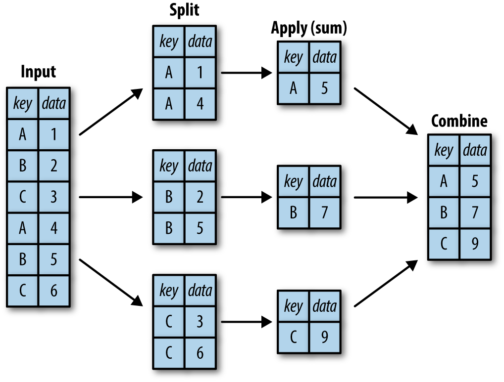
While we could certainly do this manually using some combination of
the masking, aggregation, and merging commands covered earlier, it’s
important to realize that the intermediate splits do not need to be
explicitly instantiated. Rather, the GroupBy can (often) do this in a
single pass over the data, updating the sum, mean, count, min, or other
aggregate for each group along the way. The power of the GroupBy is that
it abstracts away these steps: the user need not think about how the
computation is done under the hood, but rather thinks about the
operation as a whole.
As a concrete example, let’s take a look at using Pandas for the computation
shown in Figure 3-1. We’ll start by creating the input DataFrame:
In[11]:df=pd.DataFrame({'key':['A','B','C','A','B','C'],'data':range(6)},columns=['key','data'])df
Out[11]: key data
0 A 0
1 B 1
2 C 2
3 A 3
4 B 4
5 C 5
We can compute the most basic split-apply-combine operation with the
groupby() method of DataFrames, passing the name of the desired key
column:
In[12]:df.groupby('key')
Out[12]: <pandas.core.groupby.DataFrameGroupBy object at 0x117272160>
Notice that what is returned is not a set of DataFrames, but a
DataFrameGroupBy object. This object is where the magic is: you can
think of it as a special view of the DataFrame, which is poised to dig
into the groups but does no actual computation until the aggregation is
applied. This “lazy evaluation” approach means that common aggregates
can be implemented very efficiently in a way that is almost transparent
to the user.
To produce a result, we can apply an aggregate to this
DataFrameGroupBy object, which will perform the appropriate
apply/combine steps to produce the desired result:
In[13]:df.groupby('key').sum()
Out[13]: data
key
A 3
B 5
C 7
The sum() method is just one possibility here; you can apply virtually
any common Pandas or NumPy aggregation function, as well as virtually
any valid DataFrame operation, as we will see in the following discussion.
The GroupBy object is a very flexible abstraction. In many ways, you can
simply treat it as if it’s a collection of DataFrames, and it does the
difficult things under the hood. Let’s see some examples using the
Planets data.
Perhaps the most important operations made available by a GroupBy are
aggregate, filter, transform, and apply. We’ll discuss each of these more fully in “Aggregate, filter, transform, apply”, but before that let’s introduce some of
the other functionality that can be used with the basic GroupBy
operation.
The GroupBy object supports column indexing in the same way as the
DataFrame, and returns a modified GroupBy object. For example:
In[14]:planets.groupby('method')
Out[14]: <pandas.core.groupby.DataFrameGroupBy object at 0x1172727b8>
In[15]:planets.groupby('method')['orbital_period']
Out[15]: <pandas.core.groupby.SeriesGroupBy object at 0x117272da0>
Here we’ve selected a particular Series group from the original
DataFrame group by reference to its column name. As with the GroupBy
object, no computation is done until we call some aggregate on the
object:
In[16]:planets.groupby('method')['orbital_period'].median()
Out[16]: method
Astrometry 631.180000
Eclipse Timing Variations 4343.500000
Imaging 27500.000000
Microlensing 3300.000000
Orbital Brightness Modulation 0.342887
Pulsar Timing 66.541900
Pulsation Timing Variations 1170.000000
Radial Velocity 360.200000
Transit 5.714932
Transit Timing Variations 57.011000
Name: orbital_period, dtype: float64
This gives an idea of the general scale of orbital periods (in days) that each method is sensitive to.
The GroupBy object supports direct iteration over the groups, returning
each group as a Series or DataFrame:
In[17]:for(method,group)inplanets.groupby('method'):("{0:30s} shape={1}".format(method,group.shape))
Astrometry shape=(2, 6) Eclipse Timing Variations shape=(9, 6) Imaging shape=(38, 6) Microlensing shape=(23, 6) Orbital Brightness Modulation shape=(3, 6) Pulsar Timing shape=(5, 6) Pulsation Timing Variations shape=(1, 6) Radial Velocity shape=(553, 6) Transit shape=(397, 6) Transit Timing Variations shape=(4, 6)
This can be useful for doing certain things manually, though it is often
much faster to use the built-in apply functionality, which we will
discuss momentarily.
Through some Python class magic, any method not explicitly implemented
by the GroupBy object will be passed through and called on the groups,
whether they are DataFrame or Series objects. For example, you can use
the describe() method of DataFrames to perform a set of aggregations
that describe each group in the data:
In[18]:planets.groupby('method')['year'].describe().unstack()
Out[18]:
count mean std min 25% \\
method
Astrometry 2.0 2011.500000 2.121320 2010.0 2010.75
Eclipse Timing Variations 9.0 2010.000000 1.414214 2008.0 2009.00
Imaging 38.0 2009.131579 2.781901 2004.0 2008.00
Microlensing 23.0 2009.782609 2.859697 2004.0 2008.00
Orbital Brightness Modulation 3.0 2011.666667 1.154701 2011.0 2011.00
Pulsar Timing 5.0 1998.400000 8.384510 1992.0 1992.00
Pulsation Timing Variations 1.0 2007.000000 NaN 2007.0 2007.00
Radial Velocity 553.0 2007.518987 4.249052 1989.0 2005.00
Transit 397.0 2011.236776 2.077867 2002.0 2010.00
Transit Timing Variations 4.0 2012.500000 1.290994 2011.0 2011.75
50% 75% max
method
Astrometry 2011.5 2012.25 2013.0
Eclipse Timing Variations 2010.0 2011.00 2012.0
Imaging 2009.0 2011.00 2013.0
Microlensing 2010.0 2012.00 2013.0
Orbital Brightness Modulation 2011.0 2012.00 2013.0
Pulsar Timing 1994.0 2003.00 2011.0
Pulsation Timing Variations 2007.0 2007.00 2007.0
Radial Velocity 2009.0 2011.00 2014.0
Transit 2012.0 2013.00 2014.0
Transit Timing Variations 2012.5 2013.25 2014.0
Looking at this table helps us to better understand the data: for example, the vast majority of planets have been discovered by the Radial Velocity and Transit methods, though the latter only became common (due to new, more accurate telescopes) in the last decade. The newest methods seem to be Transit Timing Variation and Orbital Brightness Modulation, which were not used to discover a new planet until 2011.
This is just one example of the utility of dispatch methods. Notice that
they are applied to each individual group, and the results are then
combined within GroupBy and returned. Again, any valid DataFrame/Series
method can be used on the corresponding GroupBy object, which allows for
some very flexible and powerful operations!
The preceding discussion focused on aggregation for the combine operation,
but there are more options available. In particular, GroupBy objects
have aggregate(), filter(), transform(), and apply() methods
that efficiently implement a variety of useful operations before
combining the grouped data.
For the purpose of the following subsections, we’ll use this
DataFrame:
In[19]:rng=np.random.RandomState(0)df=pd.DataFrame({'key':['A','B','C','A','B','C'],'data1':range(6),'data2':rng.randint(0,10,6)},columns=['key','data1','data2'])df
Out[19]: key data1 data2
0 A 0 5
1 B 1 0
2 C 2 3
3 A 3 3
4 B 4 7
5 C 5 9
We’re now familiar with GroupBy aggregations with sum(), median(),
and the like, but the aggregate() method allows for even more flexibility. It
can take a string, a function, or a list thereof, and compute all the
aggregates at once. Here is a quick example combining all these:
In[20]:df.groupby('key').aggregate(['min',np.median,max])
Out[20]: data1 data2
min median max min median max
key
A 0 1.5 3 3 4.0 5
B 1 2.5 4 0 3.5 7
C 2 3.5 5 3 6.0 9
Another useful pattern is to pass a dictionary mapping column names to operations to be applied on that column:
In[21]:df.groupby('key').aggregate({'data1':'min','data2':'max'})
Out[21]: data1 data2
key
A 0 5
B 1 7
C 2 9
A filtering operation allows you to drop data based on the group properties. For example, we might want to keep all groups in which the standard deviation is larger than some critical value:
In[22]:deffilter_func(x):returnx['data2'].std()>4(df);(df.groupby('key').std());(df.groupby('key').filter(filter_func))
df df.groupby('key').std()
key data1 data2 key data1 data2
0 A 0 5 A 2.12132 1.414214
1 B 1 0 B 2.12132 4.949747
2 C 2 3 C 2.12132 4.242641
3 A 3 3
4 B 4 7
5 C 5 9
df.groupby('key').filter(filter_func)
key data1 data2
1 B 1 0
2 C 2 3
4 B 4 7
5 C 5 9
The filter() function should return a Boolean value specifying whether the
group passes the filtering. Here because group A does not have a
standard deviation greater than 4, it is dropped from the result.
While aggregation must return a reduced version of the data, transformation can return some transformed version of the full data to recombine. For such a transformation, the output is the same shape as the input. A common example is to center the data by subtracting the group-wise mean:
In[23]:df.groupby('key').transform(lambdax:x-x.mean())
Out[23]: data1 data2
0 -1.5 1.0
1 -1.5 -3.5
2 -1.5 -3.0
3 1.5 -1.0
4 1.5 3.5
5 1.5 3.0
The apply() method lets you apply an arbitrary function to the group
results. The function should take a DataFrame, and return either a
Pandas object (e.g., DataFrame, Series) or a scalar; the combine
operation will be tailored to the type of output returned.
For example, here is an apply() that normalizes the first column by
the sum of the second:
In[24]:defnorm_by_data2(x):# x is a DataFrame of group valuesx['data1']/=x['data2'].sum()returnx(df);(df.groupby('key').apply(norm_by_data2))
df df.groupby('key').apply(norm_by_data2)
key data1 data2 key data1 data2
0 A 0 5 0 A 0.000000 5
1 B 1 0 1 B 0.142857 0
2 C 2 3 2 C 0.166667 3
3 A 3 3 3 A 0.375000 3
4 B 4 7 4 B 0.571429 7
5 C 5 9 5 C 0.416667 9
apply() within a GroupBy is quite flexible: the only criterion is that
the function takes a DataFrame and returns a Pandas object or scalar;
what you do in the middle is up to you!
In the simple examples presented before, we split the DataFrame on a single
column name. This is just one of many options by which the groups can be
defined, and we’ll go through some other options for group specification
here.
The key can be any series or list with a length matching that of the
DataFrame. For example:
In[25]:L=[0,1,0,1,2,0](df);(df.groupby(L).sum())
df df.groupby(L).sum() key data1 data2 data1 data2 0 A 0 5 0 7 17 1 B 1 0 1 4 3 2 C 2 3 2 4 7 3 A 3 3 4 B 4 7 5 C 5 9
Of course, this means there’s another, more verbose way of accomplishing
the df.groupby('key') from before:
In[26]:(df);(df.groupby(df['key']).sum())
df df.groupby(df['key']).sum() key data1 data2 data1 data2 0 A 0 5 A 3 8 1 B 1 0 B 5 7 2 C 2 3 C 7 12 3 A 3 3 4 B 4 7 5 C 5 9
Another method is to provide a dictionary that maps index values to the group keys:
In[27]:df2=df.set_index('key')mapping={'A':'vowel','B':'consonant','C':'consonant'}(df2);(df2.groupby(mapping).sum())
df2 df2.groupby(mapping).sum() key data1 data2 data1 data2 A 0 5 consonant 12 19 B 1 0 vowel 3 8 C 2 3 A 3 3 B 4 7 C 5 9
Similar to mapping, you can pass any Python function that will input the index value and output the group:
In[28]:(df2);(df2.groupby(str.lower).mean())
df2 df2.groupby(str.lower).mean() key data1 data2 data1 data2 A 0 5 a 1.5 4.0 B 1 0 b 2.5 3.5 C 2 3 c 3.5 6.0 A 3 3 B 4 7 C 5 9
Further, any of the preceding key choices can be combined to group on a multi-index:
In[29]:df2.groupby([str.lower,mapping]).mean()
Out[29]: data1 data2
a vowel 1.5 4.0
b consonant 2.5 3.5
c consonant 3.5 6.0
As an example of this, in a couple lines of Python code we can put all these together and count discovered planets by method and by decade:
In[30]:decade=10*(planets['year']//10)decade=decade.astype(str)+'s'decade.name='decade'planets.groupby(['method',decade])['number'].sum().unstack().fillna(0)
Out[30]: decade 1980s 1990s 2000s 2010s
method
Astrometry 0.0 0.0 0.0 2.0
Eclipse Timing Variations 0.0 0.0 5.0 10.0
Imaging 0.0 0.0 29.0 21.0
Microlensing 0.0 0.0 12.0 15.0
Orbital Brightness Modulation 0.0 0.0 0.0 5.0
Pulsar Timing 0.0 9.0 1.0 1.0
Pulsation Timing Variations 0.0 0.0 1.0 0.0
Radial Velocity 1.0 52.0 475.0 424.0
Transit 0.0 0.0 64.0 712.0
Transit Timing Variations 0.0 0.0 0.0 9.0
This shows the power of combining many of the operations we’ve discussed up to this point when looking at realistic datasets. We immediately gain a coarse understanding of when and how planets have been discovered over the past several decades!
Here I would suggest digging into these few lines of code, and evaluating the individual steps to make sure you understand exactly what they are doing to the result. It’s certainly a somewhat complicated example, but understanding these pieces will give you the means to similarly explore your own data.
We have seen how the GroupBy abstraction lets us explore relationships
within a dataset. A pivot table is a similar operation that is
commonly seen in spreadsheets and other programs that operate on
tabular data. The pivot table takes simple column-wise data as input,
and groups the entries into a two-dimensional table that provides a
multidimensional summarization of the data. The difference between
pivot tables and GroupBy can sometimes cause confusion; it helps me to
think of pivot tables as essentially a multidimensional version of
GroupBy aggregation. That is, you split-apply-combine, but both the
split and the combine happen across not a one-dimensional index, but
across a two-dimensional grid.
For the examples in this section, we’ll use the database of passengers on the Titanic, available through the Seaborn library (see “Visualization with Seaborn”):
In[1]:importnumpyasnpimportpandasaspdimportseabornassnstitanic=sns.load_dataset('titanic')
In[2]:titanic.head()
Out[2]:
survived pclass sex age sibsp parch fare embarked class \\
0 0 3 male 22.0 1 0 7.2500 S Third
1 1 1 female 38.0 1 0 71.2833 C First
2 1 3 female 26.0 0 0 7.9250 S Third
3 1 1 female 35.0 1 0 53.1000 S First
4 0 3 male 35.0 0 0 8.0500 S Third
who adult_male deck embark_town alive alone
0 man True NaN Southampton no False
1 woman False C Cherbourg yes False
2 woman False NaN Southampton yes True
3 woman False C Southampton yes False
4 man True NaN Southampton no True
This contains a wealth of information on each passenger of that ill-fated voyage, including gender, age, class, fare paid, and much more.
To start learning more about this data, we might begin by grouping it according to gender, survival status, or some combination thereof. If you have
read the previous section, you might be tempted to apply a GroupBy
operation—for example, let’s look at survival rate by gender:
In[3]:titanic.groupby('sex')[['survived']].mean()
Out[3]: survived
sex
female 0.742038
male 0.188908
This immediately gives us some insight: overall, three of every four females on board survived, while only one in five males survived!
This is useful, but we might like to go one step deeper and look at
survival by both sex and, say, class. Using the vocabulary of GroupBy,
we might proceed using something like this: we group by class and gender,
select survival, apply a mean aggregate, combine the resulting
groups, and then unstack the hierarchical index to reveal the hidden
multidimensionality. In code:
In[4]:titanic.groupby(['sex','class'])['survived'].aggregate('mean').unstack()
Out[4]: class First Second Third
sex
female 0.968085 0.921053 0.500000
male 0.368852 0.157407 0.135447
This gives us a better idea of how both gender and class affected
survival, but the code is starting to look a bit garbled. While each
step of this pipeline makes sense in light of the tools we’ve previously
discussed, the long string of code is not particularly easy to read or
use. This two-dimensional GroupBy is common enough that Pandas includes
a convenience routine, pivot_table, which succinctly handles this type
of multidimensional aggregation.
Here is the equivalent to the preceding operation using the pivot_table
method of DataFrames:
In[5]:titanic.pivot_table('survived',index='sex',columns='class')
Out[5]: class First Second Third
sex
female 0.968085 0.921053 0.500000
male 0.368852 0.157407 0.135447
This is eminently more readable than the GroupBy approach, and produces
the same result. As you might expect of an early 20th-century
transatlantic cruise, the survival gradient favors both women and higher
classes. First-class women survived with near certainty (hi, Rose!),
while only one in ten third-class men survived (sorry, Jack!).
Just as in the GroupBy, the grouping in pivot tables can be specified
with multiple levels, and via a number of options. For example, we might
be interested in looking at age as a third dimension. We’ll bin the age
using the pd.cut function:
In[6]:age=pd.cut(titanic['age'],[0,18,80])titanic.pivot_table('survived',['sex',age],'class')
Out[6]: class First Second Third
sex age
female (0, 18] 0.909091 1.000000 0.511628
(18, 80] 0.972973 0.900000 0.423729
male (0, 18] 0.800000 0.600000 0.215686
(18, 80] 0.375000 0.071429 0.133663
We can apply this same strategy when working with the columns as well; let’s add info on the fare
paid using pd.qcut to automatically compute quantiles:
In[7]:fare=pd.qcut(titanic['fare'],2)titanic.pivot_table('survived',['sex',age],[fare,'class'])
Out[7]:
fare [0, 14.454]
class First Second Third \\
sex age
female (0, 18] NaN 1.000000 0.714286
(18, 80] NaN 0.880000 0.444444
male (0, 18] NaN 0.000000 0.260870
(18, 80] 0.0 0.098039 0.125000
fare (14.454, 512.329]
class First Second Third
sex age
female (0, 18] 0.909091 1.000000 0.318182
(18, 80] 0.972973 0.914286 0.391304
male (0, 18] 0.800000 0.818182 0.178571
(18, 80] 0.391304 0.030303 0.192308
The result is a four-dimensional aggregation with hierarchical indices (see “Hierarchical Indexing”), shown in a grid demonstrating the relationship between the values.
The full call signature of the pivot_table method of DataFrames is as
follows:
# call signature as of Pandas 0.18DataFrame.pivot_table(data,values=None,index=None,columns=None,aggfunc='mean',fill_value=None,margins=False,dropna=True,margins_name='All')
We’ve already seen examples of the first three arguments; here we’ll take
a quick look at the remaining ones. Two of the options,
fill_value and dropna, have to do with missing data and are fairly
straightforward; we will not show examples of them here.
The aggfunc keyword controls what type of aggregation is applied,
which is a mean by default. As in the GroupBy, the aggregation
specification can be a string representing one of several common choices
('sum', 'mean', 'count', 'min', 'max', etc.) or a
function that implements an aggregation (np.sum(), min(),
sum(), etc.). Additionally, it can be specified as a dictionary mapping
a column to any of the above desired options:
In[8]:titanic.pivot_table(index='sex',columns='class',aggfunc={'survived':sum,'fare':'mean'})
Out[8]: fare survived
class First Second Third First Second Third
sex
female 106.125798 21.970121 16.118810 91.0 70.0 72.0
male 67.226127 19.741782 12.661633 45.0 17.0 47.0
Notice also here that we’ve omitted the values keyword; when you’re specifying a mapping for aggfunc, this is determined automatically.
At times it’s useful to compute totals along each grouping. This can be
done via the margins keyword:
In[9]:titanic.pivot_table('survived',index='sex',columns='class',margins=True)
Out[9]: class First Second Third All
sex
female 0.968085 0.921053 0.500000 0.742038
male 0.368852 0.157407 0.135447 0.188908
All 0.629630 0.472826 0.242363 0.383838
Here this automatically gives us information about the class-agnostic
survival rate by gender, the gender-agnostic survival rate by class, and
the overall survival rate of 38%. The margin label can be specified with
the margins_name keyword, which defaults to "All".
As a more interesting example, let’s take a look at the freely available data on births in the United States, provided by the Centers for Disease Control (CDC). This data can be found at https://raw.githubusercontent.com/jakevdp/data-CDCbirths/master/births.csv (this dataset has been analyzed rather extensively by Andrew Gelman and his group; see, for example, this blog post):
In[10]:# shell command to download the data:# !curl -O https://raw.githubusercontent.com/jakevdp/data-CDCbirths/# master/births.csv
In[11]:births=pd.read_csv('births.csv')
Taking a look at the data, we see that it’s relatively simple—it contains the number of births grouped by date and gender:
In[12]:births.head()
Out[12]: year month day gender births
0 1969 1 1 F 4046
1 1969 1 1 M 4440
2 1969 1 2 F 4454
3 1969 1 2 M 4548
4 1969 1 3 F 4548
We can start to understand this data a bit more by using a pivot table. Let’s add a decade column, and take a look at male and female births as a function of decade:
In[13]:births['decade']=10*(births['year']//10)births.pivot_table('births',index='decade',columns='gender',aggfunc='sum')
Out[13]: gender F M
decade
1960 1753634 1846572
1970 16263075 17121550
1980 18310351 19243452
1990 19479454 20420553
2000 18229309 19106428
We immediately see that male births outnumber female births in every decade. To see this trend a bit more clearly, we can use the built-in plotting tools in Pandas to visualize the total number of births by year (Figure 3-2; see Chapter 4 for a discussion of plotting with Matplotlib):
In[14]:%matplotlibinlineimportmatplotlib.pyplotaspltsns.set()# use Seaborn stylesbirths.pivot_table('births',index='year',columns='gender',aggfunc='sum').plot()plt.ylabel('total births per year');
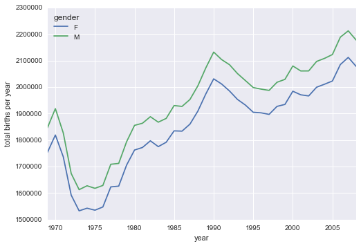
With a simple pivot table and plot() method, we can immediately see
the annual trend in births by gender. By eye, it appears that over the
past 50 years male births have outnumbered female births by around 5%.
Though this doesn’t necessarily relate to the pivot table, there are a few more interesting features we can pull out of this dataset using the Pandas tools covered up to this point. We must start by cleaning the data a bit, removing outliers caused by mistyped dates (e.g., June 31st) or missing values (e.g., June 99th). One easy way to remove these all at once is to cut outliers; we’ll do this via a robust sigma-clipping operation:1
In[15]:quartiles=np.percentile(births['births'],[25,50,75])mu=quartiles[1]sig=0.74*(quartiles[2]-quartiles[0])
This final line is a robust estimate of the sample mean, where the 0.74
comes from the interquartile range of a Gaussian distribution. With this
we can use the query() method (discussed further in
“High-Performance Pandas: eval() and query()”) to filter out rows with births outside these
values:
In[16]:births=births.query('(births > @mu - 5 * @sig) & (births < @mu + 5 * @sig)')
Next we set the day column to integers; previously it had been a
string because some columns in the dataset contained the value 'null':
In[17]:# set 'day' column to integer; it originally was a string due to nullsbirths['day']=births['day'].astype(int)
Finally, we can combine the day, month, and year to create a Date index (see “Working with Time Series”). This allows us to quickly compute the weekday corresponding to each row:
In[18]:# create a datetime index from the year, month, daybirths.index=pd.to_datetime(10000*births.year+100*births.month+births.day,format='%Y%m%d')births['dayofweek']=births.index.dayofweek
Using this we can plot births by weekday for several decades (Figure 3-3):
In[19]:importmatplotlib.pyplotaspltimportmatplotlibasmplbirths.pivot_table('births',index='dayofweek',columns='decade',aggfunc='mean').plot()plt.gca().set_xticklabels(['Mon','Tues','Wed','Thurs','Fri','Sat','Sun'])plt.ylabel('mean births by day');
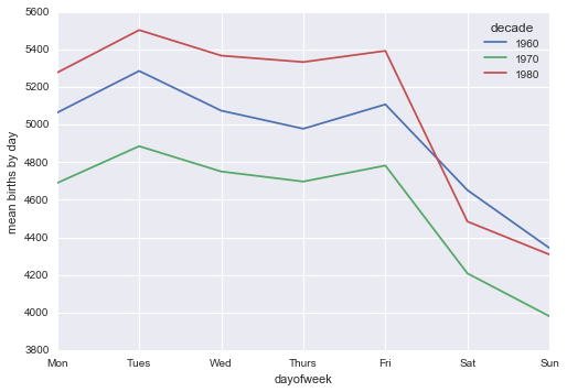
Apparently births are slightly less common on weekends than on weekdays! Note that the 1990s and 2000s are missing because the CDC data contains only the month of birth starting in 1989.
Another interesting view is to plot the mean number of births by the day of the year. Let’s first group the data by month and day separately:
In[20]:births_by_date=births.pivot_table('births',[births.index.month,births.index.day])births_by_date.head()
Out[20]: 1 1 4009.225
2 4247.400
3 4500.900
4 4571.350
5 4603.625
Name: births, dtype: float64
The result is a multi-index over months and days. To make this easily plottable, let’s turn these months and days into a date by associating them with a dummy year variable (making sure to choose a leap year so February 29th is correctly handled!)
In[21]:births_by_date.index=[pd.datetime(2012,month,day)for(month,day)inbirths_by_date.index]births_by_date.head()
Out[21]: 2012-01-01 4009.225
2012-01-02 4247.400
2012-01-03 4500.900
2012-01-04 4571.350
2012-01-05 4603.625
Name: births, dtype: float64
Focusing on the month and day only, we now have a time series reflecting
the average number of births by date of the year. From this, we can use
the plot method to plot the data (Figure 3-4). It reveals some interesting trends:
In[22]:# Plot the resultsfig,ax=plt.subplots(figsize=(12,4))births_by_date.plot(ax=ax);
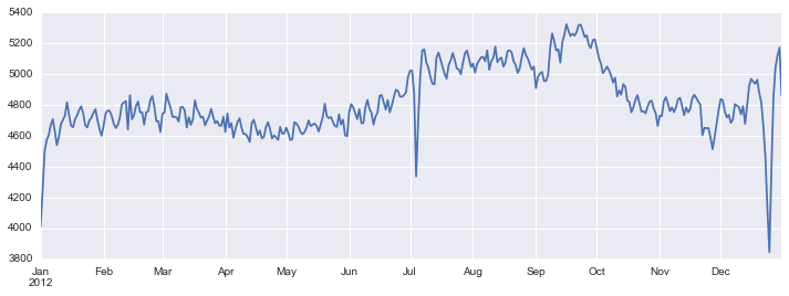
In particular, the striking feature of this graph is the dip in birthrate on US holidays (e.g., Independence Day, Labor Day, Thanksgiving, Christmas, New Year’s Day) although this likely reflects trends in scheduled/induced births rather than some deep psychosomatic effect on natural births. For more discussion on this trend, see the analysis and links in Andrew Gelman’s blog post on the subject. We’ll return to this figure in “Example: Effect of Holidays on US Births”, where we will use Matplotlib’s tools to annotate this plot.
Looking at this short example, you can see that many of the Python and Pandas tools we’ve seen to this point can be combined and used to gain insight from a variety of datasets. We will see some more sophisticated applications of these data manipulations in future sections!
One strength of Python is its relative ease in handling and manipulating string data. Pandas builds on this and provides a comprehensive set of vectorized string operations that become an essential piece of the type of munging required when one is working with (read: cleaning up) real-world data. In this section, we’ll walk through some of the Pandas string operations, and then take a look at using them to partially clean up a very messy dataset of recipes collected from the Internet.
We saw in previous sections how tools like NumPy and Pandas generalize arithmetic operations so that we can easily and quickly perform the same operation on many array elements. For example:
In[1]:importnumpyasnpx=np.array([2,3,5,7,11,13])x*2
Out[1]: array([ 4, 6, 10, 14, 22, 26])
This vectorization of operations simplifies the syntax of operating on arrays of data: we no longer have to worry about the size or shape of the array, but just about what operation we want done. For arrays of strings, NumPy does not provide such simple access, and thus you’re stuck using a more verbose loop syntax:
In[2]:data=['peter','Paul','MARY','gUIDO'][s.capitalize()forsindata]
Out[2]: ['Peter', 'Paul', 'Mary', 'Guido']
This is perhaps sufficient to work with some data, but it will break if there are any missing values. For example:
In[3]:data=['peter','Paul',None,'MARY','gUIDO'][s.capitalize()forsindata]
---------------------------------------------------------------------------
---------------------------------------------------------------------------
AttributeError Traceback (most recent call last)
<ipython-input-3-fc1d891ab539> in <module>()
1 data = ['peter', 'Paul', None, 'MARY', 'gUIDO']
----> 2 [s.capitalize() for s in data]
<ipython-input-3-fc1d891ab539> in <listcomp>(.0)
1 data = ['peter', 'Paul', None, 'MARY', 'gUIDO']
----> 2 [s.capitalize() for s in data]
AttributeError: 'NoneType' object has no attribute 'capitalize'
---------------------------------------------------------------------------
Pandas includes features to address both this need for vectorized string
operations and for correctly handling missing data via the str
attribute of Pandas Series and Index objects containing strings. So, for
example, suppose we create a Pandas Series with this data:
In[4]:importpandasaspdnames=pd.Series(data)names
Out[4]: 0 peter
1 Paul
2 None
3 MARY
4 gUIDO
dtype: object
We can now call a single method that will capitalize all the entries, while skipping over any missing values:
In[5]:names.str.capitalize()
Out[5]: 0 Peter
1 Paul
2 None
3 Mary
4 Guido
dtype: object
Using tab completion on this str attribute will list all the
vectorized string methods available to Pandas.
If you have a good understanding of string manipulation in Python, most of Pandas’ string syntax is intuitive enough that it’s probably sufficient to just list a table of available methods; we will start with that here, before diving deeper into a few of the subtleties. The examples in this section use the following series of names:
In[6]:monte=pd.Series(['Graham Chapman','John Cleese','Terry Gilliam','Eric Idle','Terry Jones','Michael Palin'])
Nearly all Python’s built-in string methods are mirrored by a Pandas
vectorized string method. Here is a list of Pandas str methods that
mirror Python string methods:
|
|
|
|
|
|
|
|
|
|
|
|
|
|
|
|
|
|
|
|
|
|
|
|
|
|
|
|
|
|
|
|
Notice that these have various return values. Some, like lower(), return a series of strings:
In[7]:monte.str.lower()
Out[7]: 0 graham chapman
1 john cleese
2 terry gilliam
3 eric idle
4 terry jones
5 michael palin
dtype: object
But some others return numbers:
In[8]:monte.str.len()
Out[8]: 0 14
1 11
2 13
3 9
4 11
5 13
dtype: int64
Or Boolean values:
In[9]:monte.str.startswith('T')
Out[9]: 0 False
1 False
2 True
3 False
4 True
5 False
dtype: bool
Still others return lists or other compound values for each element:
In[10]:monte.str.split()
Out[10]: 0 [Graham, Chapman]
1 [John, Cleese]
2 [Terry, Gilliam]
3 [Eric, Idle]
4 [Terry, Jones]
5 [Michael, Palin]
dtype: object
We’ll see further manipulations of this kind of series-of-lists object as we continue our discussion.
In addition, there are several methods that accept regular expressions
to examine the content of each string element, and follow some of the
API conventions of Python’s built-in re module (see Table 3-4).
| Method | Description |
|---|---|
|
Call |
|
Call |
|
Call |
|
Replace occurrences of pattern with some other string. |
|
Call |
|
Count occurrences of pattern. |
|
Equivalent to |
|
Equivalent to |
With these, you can do a wide range of interesting operations. For example, we can extract the first name from each by asking for a contiguous group of characters at the beginning of each element:
In[11]:monte.str.extract('([A-Za-z]+)')
Out[11]: 0 Graham
1 John
2 Terry
3 Eric
4 Terry
5 Michael
dtype: object
Or we can do something more complicated, like finding all names that
start and end with a consonant, making use of the start-of-string
(^) and end-of-string ($) regular expression characters:
In[12]:monte.str.findall(r'^[^AEIOU].*[^aeiou]$')
Out[12]: 0 [Graham Chapman]
1 []
2 [Terry Gilliam]
3 []
4 [Terry Jones]
5 [Michael Palin]
dtype: object
The ability to concisely apply regular expressions across Series or
DataFrame entries opens up many possibilities for analysis and cleaning
of data.
Finally, there are some miscellaneous methods that enable other convenient operations (see Table 3-5).
| Method | Description |
|---|---|
|
Index each element |
|
Slice each element |
|
Replace slice in each element with passed value |
|
Concatenate strings |
|
Repeat values |
|
Return Unicode form of string |
|
Add whitespace to left, right, or both sides of strings |
|
Split long strings into lines with length less than a given width |
|
Join strings in each element of the |
|
Extract dummy variables as a |
The get() and slice() operations, in particular, enable vectorized
element access from each array. For example, we can get a slice of the
first three characters of each array using str.slice(0, 3). Note that
this behavior is also available through Python’s normal indexing syntax—for example, df.str.slice(0, 3) is equivalent to df.str[0:3]:
In[13]:monte.str[0:3]
Out[13]: 0 Gra
1 Joh
2 Ter
3 Eri
4 Ter
5 Mic
dtype: object
Indexing via df.str.get(i) and df.str[i] is similar.
These get() and slice() methods also let you access elements of
arrays returned by split(). For example, to extract the last
name of each entry, we can combine split() and get():
In[14]:monte.str.split().str.get(-1)
Out[14]: 0 Chapman
1 Cleese
2 Gilliam
3 Idle
4 Jones
5 Palin
dtype: object
Another method that requires a bit of extra explanation is the
get_dummies() method. This is useful when your data has a column
containing some sort of coded indicator. For example, we might have a
dataset that contains information in the form of codes, such as A=“born
in America,” B=“born in the United Kingdom,” C=“likes cheese,” D=“likes
spam”:
In[15]:full_monte=pd.DataFrame({'name':monte,'info':['B|C|D','B|D','A|C','B|D','B|C','B|C|D']})full_monte
Out[15]: info name
0 B|C|D Graham Chapman
1 B|D John Cleese
2 A|C Terry Gilliam
3 B|D Eric Idle
4 B|C Terry Jones
5 B|C|D Michael Palin
The get_dummies() routine lets you quickly split out these indicator
variables into a DataFrame:
In[16]:full_monte['info'].str.get_dummies('|')
Out[16]: A B C D
0 0 1 1 1
1 0 1 0 1
2 1 0 1 0
3 0 1 0 1
4 0 1 1 0
5 0 1 1 1
With these operations as building blocks, you can construct an endless range of string processing procedures when cleaning your data.
We won’t dive further into these methods here, but I encourage you to
read through “Working with Text Data” in the pandas online documentation, or to refer to the resources listed in
“Further Resources”.
These vectorized string operations become most useful in the process of cleaning up messy, real-world data. Here I’ll walk through an example of that, using an open recipe database compiled from various sources on the Web. Our goal will be to parse the recipe data into ingredient lists, so we can quickly find a recipe based on some ingredients we have on hand.
The scripts used to compile this can be found at https://github.com/fictivekin/openrecipes, and the link to the current version of the database is found there as well.
As of spring 2016, this database is about 30 MB, and can be downloaded and unzipped with these commands:
In[17]:# !curl -O http://openrecipes.s3.amazonaws.com/recipeitems-latest.json.gz# !gunzip recipeitems-latest.json.gz
The database is in JSON format, so we will try pd.read_json to read it:
In[18]:try:recipes=pd.read_json('recipeitems-latest.json')exceptValueErrorase:("ValueError:",e)
ValueError: Trailing data
Oops! We get a ValueError mentioning that there is “trailing data.”
Searching for this error on the Internet, it seems that it’s due to
using a file in which each line is itself a valid JSON, but the full
file is not. Let’s check if this interpretation is true:
In[19]:withopen('recipeitems-latest.json')asf:line=f.readline()pd.read_json(line).shape
Out[19]: (2, 12)
Yes, apparently each line is a valid JSON, so we’ll need to string them
together. One way we can do this is to actually construct a string
representation containing all these JSON entries, and then load the
whole thing with pd.read_json:
In[20]:# read the entire file into a Python arraywithopen('recipeitems-latest.json','r')asf:# Extract each linedata=(line.strip()forlineinf)# Reformat so each line is the element of a listdata_json="[{0}]".format(','.join(data))# read the result as a JSONrecipes=pd.read_json(data_json)
In[21]:recipes.shape
Out[21]: (173278, 17)
We see there are nearly 200,000 recipes, and 17 columns. Let’s take a look at one row to see what we have:
In[22]:recipes.iloc[0]
Out[22]:
_id {'$oid': '5160756b96cc62079cc2db15'}
cookTime PT30M
creator NaN
dateModified NaN
datePublished 2013-03-11
description Late Saturday afternoon, after Marlboro Man ha...
image http://static.thepioneerwoman.com/cooking/file...
ingredients Biscuits\n3 cups All-purpose Flour\n2 Tablespo...
name Drop Biscuits and Sausage Gravy
prepTime PT10M
recipeCategory NaN
recipeInstructions NaN
recipeYield 12
source thepioneerwoman
totalTime NaN
ts {'$date': 1365276011104}
url http://thepioneerwoman.com/cooking/2013/03/dro...
Name: 0, dtype: object
There is a lot of information there, but much of it is in a very messy form, as is typical of data scraped from the Web. In particular, the ingredient list is in string format; we’re going to have to carefully extract the information we’re interested in. Let’s start by taking a closer look at the ingredients:
In[23]:recipes.ingredients.str.len().describe()
Out[23]: count 173278.000000
mean 244.617926
std 146.705285
min 0.000000
25% 147.000000
50% 221.000000
75% 314.000000
max 9067.000000
Name: ingredients, dtype: float64
The ingredient lists average 250 characters long, with a minimum of 0 and a maximum of nearly 10,000 characters!
Just out of curiosity, let’s see which recipe has the longest ingredient list:
In[24]:recipes.name[np.argmax(recipes.ingredients.str.len())]
Out[24]: 'Carrot Pineapple Spice & Brownie Layer Cake with Whipped Cream & Cream Cheese Frosting and Marzipan Carrots'
That certainly looks like an involved recipe.
We can do other aggregate explorations; for example, let’s see how many of the recipes are for breakfast food:
In[33]:recipes.description.str.contains('[Bb]reakfast').sum()
Out[33]: 3524
Or how many of the recipes list cinnamon as an ingredient:
In[34]:recipes.ingredients.str.contains('[Cc]innamon').sum()
Out[34]: 10526
We could even look to see whether any recipes misspell the ingredient as “cinamon”:
In[27]:recipes.ingredients.str.contains('[Cc]inamon').sum()
Out[27]: 11
This is the type of essential data exploration that is possible with Pandas string tools. It is data munging like this that Python really excels at.
Let’s go a bit further, and start working on a simple recipe recommendation system: given a list of ingredients, find a recipe that uses all those ingredients. While conceptually straightforward, the task is complicated by the heterogeneity of the data: there is no easy operation, for example, to extract a clean list of ingredients from each row. So we will cheat a bit: we’ll start with a list of common ingredients, and simply search to see whether they are in each recipe’s ingredient list. For simplicity, let’s just stick with herbs and spices for the time being:
In[28]:spice_list=['salt','pepper','oregano','sage','parsley','rosemary','tarragon','thyme','paprika','cumin']
We can then build a Boolean DataFrame consisting of True and False
values, indicating whether this ingredient appears in the list:
In[29]:importrespice_df=pd.DataFrame(dict((spice,recipes.ingredients.str.contains(spice,re.IGNORECASE))forspiceinspice_list))spice_df.head()
Out[29]: cumin oregano paprika parsley pepper rosemary sage salt tarragon thyme 0 False False False False False False True False False False 1 False False False False False False False False False False 2 True False False False True False False True False False 3 False False False False False False False False False False 4 False False False False False False False False False False
Now, as an example, let’s say we’d like to find a recipe that uses
parsley, paprika, and tarragon. We can compute this very quickly using
the query() method of DataFrames, discussed in
“High-Performance Pandas: eval() and query()”:
In[30]:selection=spice_df.query('parsley & paprika & tarragon')len(selection)
Out[30]: 10
We find only 10 recipes with this combination; let’s use the index returned by this selection to discover the names of the recipes that have this combination:
In[31]:recipes.name[selection.index]
Out[31]: 2069 All cremat with a Little Gem, dandelion and wa...
74964 Lobster with Thermidor butter
93768 Burton's Southern Fried Chicken with White Gravy
113926 Mijo's Slow Cooker Shredded Beef
137686 Asparagus Soup with Poached Eggs
140530 Fried Oyster Po’boys
158475 Lamb shank tagine with herb tabbouleh
158486 Southern fried chicken in buttermilk
163175 Fried Chicken Sliders with Pickles + Slaw
165243 Bar Tartine Cauliflower Salad
Name: name, dtype: object
Now that we have narrowed down our recipe selection by a factor of almost 20,000, we are in a position to make a more informed decision about what we’d like to cook for dinner.
Hopefully this example has given you a bit of a flavor (ba-dum!) for the types of data cleaning operations that are efficiently enabled by Pandas string methods. Of course, building a very robust recipe recommendation system would require a lot more work! Extracting full ingredient lists from each recipe would be an important piece of the task; unfortunately, the wide variety of formats used makes this a relatively time-consuming process. This points to the truism that in data science, cleaning and munging of real-world data often comprises the majority of the work, and Pandas provides the tools that can help you do this efficiently.
Pandas was developed in the context of financial modeling, so as you might expect, it contains a fairly extensive set of tools for working with dates, times, and time-indexed data. Date and time data comes in a few flavors, which we will discuss here:
Time stamps reference particular moments in time (e.g., July 4th, 2015, at 7:00 a.m.).
Time intervals and periods reference a length of time between a particular beginning and end point—for example, the year 2015. Periods usually reference a special case of time intervals in which each interval is of uniform length and does not overlap (e.g., 24 hour-long periods constituting days).
Time deltas or durations reference an exact length of time (e.g., a duration of 22.56 seconds).
In this section, we will introduce how to work with each of these types of date/time data in Pandas. This short section is by no means a complete guide to the time series tools available in Python or Pandas, but instead is intended as a broad overview of how you as a user should approach working with time series. We will start with a brief discussion of tools for dealing with dates and times in Python, before moving more specifically to a discussion of the tools provided by Pandas. After listing some resources that go into more depth, we will review some short examples of working with time series data in Pandas.
The Python world has a number of available representations of dates, times, deltas, and timespans. While the time series tools provided by Pandas tend to be the most useful for data science applications, it is helpful to see their relationship to other packages used in Python.
Python’s basic objects for working with dates and times reside in the
built-in datetime module. Along with the third-party dateutil
module, you can use it to quickly perform a host of useful
functionalities on dates and times. For example, you can manually build
a date using the datetime type:
In[1]:fromdatetimeimportdatetimedatetime(year=2015,month=7,day=4)
Out[1]: datetime.datetime(2015, 7, 4, 0, 0)
Or, using the dateutil module, you can parse dates from a variety of
string formats:
In[2]:fromdateutilimportparserdate=parser.parse("4th of July, 2015")date
Out[2]: datetime.datetime(2015, 7, 4, 0, 0)
Once you have a datetime object, you can do things like printing the
day of the week:
In[3]:date.strftime('%A')
Out[3]: 'Saturday'
In the final line, we’ve used one of the standard string format codes
for printing dates ("%A"), which you can read about in the
strftime
section of Python’s
datetime documentation.
Documentation of other useful date utilities can be found in
dateutil’s online documentation. A
related package to be aware of is pytz,
which contains tools for working with the most migraine-inducing piece of
time series data: time zones.
The power of datetime and dateutil lies in their flexibility and easy
syntax: you can use these objects and their built-in methods to easily
perform nearly any operation you might be interested in. Where they
break down is when you wish to work with large arrays of dates and
times: just as lists of Python numerical variables are suboptimal
compared to NumPy-style typed numerical arrays, lists of Python datetime
objects are suboptimal compared to typed arrays of encoded dates.
The weaknesses of Python’s datetime format inspired the NumPy team to
add a set of native time series data type to NumPy. The datetime64
dtype encodes dates as 64-bit integers, and thus allows arrays of dates
to be represented very compactly. The datetime64 requires a very
specific input format:
In[4]:importnumpyasnpdate=np.array('2015-07-04',dtype=np.datetime64)date
Out[4]: array(datetime.date(2015, 7, 4), dtype='datetime64[D]')
Once we have this date formatted, however, we can quickly do vectorized operations on it:
In[5]:date+np.arange(12)
Out[5]:
array(['2015-07-04', '2015-07-05', '2015-07-06', '2015-07-07',
'2015-07-08', '2015-07-09', '2015-07-10', '2015-07-11',
'2015-07-12', '2015-07-13', '2015-07-14', '2015-07-15'],
dtype='datetime64[D]')
Because of the uniform type in NumPy datetime64 arrays, this type of
operation can be accomplished much more quickly than if we were working
directly with Python’s datetime objects, especially as arrays get
large (we introduced this type of vectorization in
“Computation on NumPy Arrays: Universal Functions”).
One detail of the datetime64 and timedelta64 objects is that they
are built on a fundamental time unit. Because the datetime64 object
is limited to 64-bit precision, the range of encodable times is 264 times this fundamental unit. In other words,
datetime64 imposes a trade-off between time resolution and maximum
time span.
For example, if you want a time resolution of one nanosecond, you only have enough information to encode a range of 264 nanoseconds, or just under 600 years. NumPy will infer the desired unit from the input; for example, here is a day-based datetime:
In[6]:np.datetime64('2015-07-04')
Out[6]: numpy.datetime64('2015-07-04')
Here is a minute-based datetime:
In[7]:np.datetime64('2015-07-04 12:00')
Out[7]: numpy.datetime64('2015-07-04T12:00')
Notice that the time zone is automatically set to the local time on the computer executing the code. You can force any desired fundamental unit using one of many format codes; for example, here we’ll force a nanosecond-based time:
In[8]:np.datetime64('2015-07-04 12:59:59.50','ns')
Out[8]: numpy.datetime64('2015-07-04T12:59:59.500000000')
Table 3-6, drawn from the NumPy datetime64 documentation, lists the available format codes along with the relative and absolute timespans that they can encode.
| Code | Meaning | Time span (relative) | Time span (absolute) |
|---|---|---|---|
|
Year |
± 9.2e18 years |
[9.2e18 BC, 9.2e18 AD] |
|
Month |
± 7.6e17 years |
[7.6e17 BC, 7.6e17 AD] |
|
Week |
± 1.7e17 years |
[1.7e17 BC, 1.7e17 AD] |
|
Day |
± 2.5e16 years |
[2.5e16 BC, 2.5e16 AD] |
|
Hour |
± 1.0e15 years |
[1.0e15 BC, 1.0e15 AD] |
|
Minute |
± 1.7e13 years |
[1.7e13 BC, 1.7e13 AD] |
|
Second |
± 2.9e12 years |
[ 2.9e9 BC, 2.9e9 AD] |
|
Millisecond |
± 2.9e9 years |
[ 2.9e6 BC, 2.9e6 AD] |
|
Microsecond |
± 2.9e6 years |
[290301 BC, 294241 AD] |
|
Nanosecond |
± 292 years |
[ 1678 AD, 2262 AD] |
|
Picosecond |
± 106 days |
[ 1969 AD, 1970 AD] |
|
Femtosecond |
± 2.6 hours |
[ 1969 AD, 1970 AD] |
|
Attosecond |
± 9.2 seconds |
[ 1969 AD, 1970 AD] |
For the types of data we see in the real world, a useful default is
datetime64[ns], as it can encode a useful range of modern dates with a
suitably fine precision.
Finally, we will note that while the datetime64 data type addresses
some of the deficiencies of the built-in Python datetime type, it
lacks many of the convenient methods and functions provided by
datetime and especially dateutil. More information can be found in
NumPy’s
datetime64 documentation.
Pandas builds upon all the tools just discussed to provide a Timestamp object,
which combines the ease of use of datetime and dateutil with the
efficient storage and vectorized interface of numpy.datetime64. From a
group of these Timestamp objects, Pandas can construct a
DatetimeIndex that can be used to index data in a Series or
DataFrame; we’ll see many examples of this below.
For example, we can use Pandas tools to repeat the demonstration from above. We can parse a flexibly formatted string date, and use format codes to output the day of the week:
In[9]:importpandasaspddate=pd.to_datetime("4th of July, 2015")date
Out[9]: Timestamp('2015-07-04 00:00:00')
In[10]:date.strftime('%A')
Out[10]: 'Saturday'
Additionally, we can do NumPy-style vectorized operations directly on this same object:
In[11]:date+pd.to_timedelta(np.arange(12),'D')
Out[11]: DatetimeIndex(['2015-07-04', '2015-07-05', '2015-07-06', '2015-07-07',
'2015-07-08', '2015-07-09', '2015-07-10', '2015-07-11',
'2015-07-12', '2015-07-13', '2015-07-14', '2015-07-15'],
dtype='datetime64[ns]', freq=None)
In the next section, we will take a closer look at manipulating time series data with the tools provided by Pandas.
Where the Pandas time series tools really become useful is when you begin
to index data by timestamps. For example, we can construct a Series
object that has time-indexed data:
In[12]:index=pd.DatetimeIndex(['2014-07-04','2014-08-04','2015-07-04','2015-08-04'])data=pd.Series([0,1,2,3],index=index)data
Out[12]: 2014-07-04 0
2014-08-04 1
2015-07-04 2
2015-08-04 3
dtype: int64
Now that we have this data in a Series, we can make use of any of the
Series indexing patterns we discussed in previous sections, passing
values that can be coerced into dates:
In[13]:data['2014-07-04':'2015-07-04']
Out[13]: 2014-07-04 0
2014-08-04 1
2015-07-04 2
dtype: int64
There are additional special date-only indexing operations, such as passing a year to obtain a slice of all data from that year:
In[14]:data['2015']
Out[14]: 2015-07-04 2
2015-08-04 3
dtype: int64
Later, we will see additional examples of the convenience of dates-as-indices. But first, let’s take a closer look at the available time series data structures.
This section will introduce the fundamental Pandas data structures for working with time series data:
For time stamps, Pandas provides the Timestamp type. As mentioned
before, it is essentially a replacement for Python’s native datetime,
but is based on the more efficient numpy.datetime64 data type. The
associated index structure is DatetimeIndex.
For time periods, Pandas provides the Period type. This encodes a
fixed-frequency interval based on numpy.datetime64. The associated
index structure is PeriodIndex.
For time deltas or durations, Pandas provides the Timedelta
type. Timedelta is a more efficient replacement for Python’s native
datetime.timedelta type, and is based on numpy.timedelta64. The
associated index structure is TimedeltaIndex.
The most fundamental of these date/time objects are the Timestamp and
DatetimeIndex objects. While these class objects can be invoked
directly, it is more common to use the pd.to_datetime() function,
which can parse a wide variety of formats. Passing a single date to
pd.to_datetime() yields a Timestamp; passing a series of dates by
default yields a DatetimeIndex:
In[15]:dates=pd.to_datetime([datetime(2015,7,3),'4th of July, 2015','2015-Jul-6','07-07-2015','20150708'])dates
Out[15]: DatetimeIndex(['2015-07-03', '2015-07-04', '2015-07-06', '2015-07-07',
'2015-07-08'],
dtype='datetime64[ns]', freq=None)
Any DatetimeIndex can be converted to a PeriodIndex with the
to_period() function with the addition of a frequency code; here we’ll
use 'D' to indicate daily frequency:
In[16]:dates.to_period('D')
Out[16]: PeriodIndex(['2015-07-03', '2015-07-04', '2015-07-06', '2015-07-07',
'2015-07-08'],
dtype='int64', freq='D')
A TimedeltaIndex is created, for example, when one date is subtracted from
another:
In[17]:dates-dates[0]
Out[17]:
TimedeltaIndex(['0 days', '1 days', '3 days', '4 days', '5 days'],
dtype='timedelta64[ns]', freq=None)
To make the creation of regular date sequences more convenient, Pandas
offers a few functions for this purpose: pd.date_range() for
timestamps, pd.period_range() for periods, and pd.timedelta_range()
for time deltas. We’ve seen that Python’s range() and NumPy’s
np.arange() turn a startpoint, endpoint, and optional stepsize into a
sequence. Similarly, pd.date_range() accepts a start date, an end
date, and an optional frequency code to create a regular sequence of
dates. By default, the frequency is one day:
In[18]:pd.date_range('2015-07-03','2015-07-10')
Out[18]: DatetimeIndex(['2015-07-03', '2015-07-04', '2015-07-05', '2015-07-06',
'2015-07-07', '2015-07-08', '2015-07-09', '2015-07-10'],
dtype='datetime64[ns]', freq='D')
Alternatively, the date range can be specified not with a start- and endpoint, but with a startpoint and a number of periods:
In[19]:pd.date_range('2015-07-03',periods=8)
Out[19]: DatetimeIndex(['2015-07-03', '2015-07-04', '2015-07-05', '2015-07-06',
'2015-07-07', '2015-07-08', '2015-07-09', '2015-07-10'],
dtype='datetime64[ns]', freq='D')
You can modify the spacing by altering the freq argument, which
defaults to D. For example, here we will construct a range of hourly
timestamps:
In[20]:pd.date_range('2015-07-03',periods=8,freq='H')
Out[20]: DatetimeIndex(['2015-07-03 00:00:00', '2015-07-03 01:00:00',
'2015-07-03 02:00:00', '2015-07-03 03:00:00',
'2015-07-03 04:00:00', '2015-07-03 05:00:00',
'2015-07-03 06:00:00', '2015-07-03 07:00:00'],
dtype='datetime64[ns]', freq='H')
To create regular sequences of period or time delta values, the very
similar pd.period_range() and pd.timedelta_range() functions are
useful. Here are some monthly periods:
In[21]:pd.period_range('2015-07',periods=8,freq='M')
Out[21]:
PeriodIndex(['2015-07', '2015-08', '2015-09', '2015-10', '2015-11', '2015-12',
'2016-01', '2016-02'],
dtype='int64', freq='M')
And a sequence of durations increasing by an hour:
In[22]:pd.timedelta_range(0,periods=10,freq='H')
Out[22]:
TimedeltaIndex(['00:00:00', '01:00:00', '02:00:00', '03:00:00', '04:00:00',
'05:00:00', '06:00:00', '07:00:00', '08:00:00', '09:00:00'],
dtype='timedelta64[ns]', freq='H')
All of these require an understanding of Pandas frequency codes, which we’ll summarize in the next section.
Fundamental to these Pandas time series tools is the concept of a
frequency or date offset. Just as we saw the D (day) and H
(hour) codes previously, we can use such codes to specify any desired
frequency spacing. Table 3-7 summarizes the main codes available.
| Code | Description | Code | Description |
|---|---|---|---|
|
Calendar day |
|
Business day |
|
Weekly |
||
|
Month end |
|
Business month end |
|
Quarter end |
|
Business quarter end |
|
Year end |
|
Business year end |
|
Hours |
|
Business hours |
|
Minutes |
||
|
Seconds |
||
|
Milliseonds |
||
|
Microseconds |
||
|
Nanoseconds |
The monthly, quarterly, and annual frequencies are all marked at the end of
the specified period. Adding an S suffix to any of these marks it instead at the beginning (Table 3-8).
| Code | Description |
|---|---|
|
Month start |
|
Business month start |
|
Quarter start |
|
Business quarter start |
|
Year start |
|
Business year start |
Additionally, you can change the month used to mark any quarterly or annual code by adding a three-letter month code as a suffix:
Q-JAN, BQ-FEB, QS-MAR, BQS-APR, etc.
A-JAN, BA-FEB, AS-MAR, BAS-APR, etc.
In the same way, you can modify the split-point of the weekly frequency by adding a three-letter weekday code:
W-SUN, W-MON, W-TUE, W-WED, etc.
On top of this, codes can be combined with numbers to specify other
frequencies. For example, for a frequency of 2 hours 30 minutes, we can
combine the hour (H) and minute (T) codes as follows:
In[23]:pd.timedelta_range(0,periods=9,freq="2H30T")
Out[23]:
TimedeltaIndex(['00:00:00', '02:30:00', '05:00:00', '07:30:00', '10:00:00',
'12:30:00', '15:00:00', '17:30:00', '20:00:00'],
dtype='timedelta64[ns]', freq='150T')
All of these short codes refer to specific instances of Pandas time
series offsets, which can be found in the pd.tseries.offsets module.
For example, we can create a business day offset directly as follows:
In[24]:frompandas.tseries.offsetsimportBDaypd.date_range('2015-07-01',periods=5,freq=BDay())
Out[24]: DatetimeIndex(['2015-07-01', '2015-07-02', '2015-07-03', '2015-07-06',
'2015-07-07'],
dtype='datetime64[ns]', freq='B')
For more discussion of the use of frequencies and offsets, see the “DateOffset objects” section of the Pandas online documentation.
The ability to use dates and times as indices to intuitively organize and access data is an important piece of the Pandas time series tools. The benefits of indexed data in general (automatic alignment during operations, intuitive data slicing and access, etc.) still apply, and Pandas provides several additional time series–specific operations.
We will take a look at a few of those here, using some stock price data
as an example. Because Pandas was developed largely in a finance
context, it includes some very specific tools for financial data. For
example, the accompanying pandas-datareader package (installable via
conda install pandas-datareader) knows how to import financial data
from a number of available sources, including Yahoo finance, Google
Finance, and others. Here we will load Google’s closing price history:
In[25]:frompandas_datareaderimportdatagoog=data.DataReader('GOOG',start='2004',end='2016',data_source='google')goog.head()
Out[25]: Open High Low Close Volume
Date
2004-08-19 49.96 51.98 47.93 50.12 NaN
2004-08-20 50.69 54.49 50.20 54.10 NaN
2004-08-23 55.32 56.68 54.47 54.65 NaN
2004-08-24 55.56 55.74 51.73 52.38 NaN
2004-08-25 52.43 53.95 51.89 52.95 NaN
For simplicity, we’ll use just the closing price:
In[26]:goog=goog['Close']
We can visualize this using the plot() method, after the normal
Matplotlib setup boilerplate (Figure 3-5):
In[27]:%matplotlibinlineimportmatplotlib.pyplotaspltimportseaborn;seaborn.set()
In[28]:goog.plot();
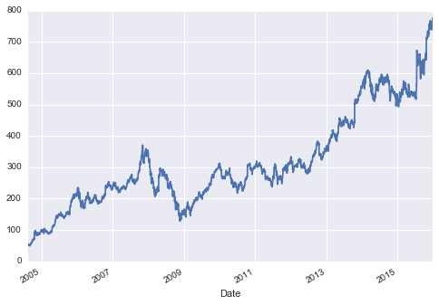
One common need for time series data is resampling at a higher or lower
frequency. You can do this using the resample() method, or the much
simpler asfreq() method. The primary difference between the two is
that resample() is fundamentally a data aggregation, while
asfreq() is fundamentally a data selection.
Taking a look at the Google closing price, let’s compare what the two return when we down-sample the data. Here we will resample the data at the end of business year (Figure 3-6):
In[29]:goog.plot(alpha=0.5,style='-')goog.resample('BA').mean().plot(style=':')goog.asfreq('BA').plot(style='--');plt.legend(['input','resample','asfreq'],loc='upper left');
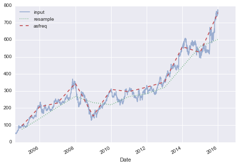
Notice the difference: at each point, resample reports the average of
the previous year, while asfreq reports the value at the end of the
year.
For up-sampling, resample() and asfreq() are largely equivalent,
though resample has many more options available. In this case, the
default for both methods is to leave the up-sampled points empty—that
is, filled with NA values. Just as with the pd.fillna() function
discussed previously, asfreq() accepts a method argument to specify
how values are imputed. Here, we will resample the business day data at
a daily frequency (i.e., including weekends); see Figure 3-7:
In[30]:fig,ax=plt.subplots(2,sharex=True)data=goog.iloc[:10]data.asfreq('D').plot(ax=ax[0],marker='o')data.asfreq('D',method='bfill').plot(ax=ax[1],style='-o')data.asfreq('D',method='ffill').plot(ax=ax[1],style='--o')ax[1].legend(["back-fill","forward-fill"]);
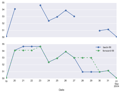
The top panel is the default: non-business days are left as NA values and do not appear on the plot. The bottom panel shows the differences between two strategies for filling the gaps: forward-filling and backward-filling.
Another common time series–specific operation is shifting of data in
time. Pandas has two closely related methods for computing this:
shift() and tshift(). In short, the difference between them is that
shift() shifts the data, while tshift() shifts the index. In
both cases, the shift is specified in multiples of the frequency.
Here we will both shift() and tshift() by 900 days (Figure 3-8):
In[31]:fig,ax=plt.subplots(3,sharey=True)# apply a frequency to the datagoog=goog.asfreq('D',method='pad')goog.plot(ax=ax[0])goog.shift(900).plot(ax=ax[1])goog.tshift(900).plot(ax=ax[2])# legends and annotationslocal_max=pd.to_datetime('2007-11-05')offset=pd.Timedelta(900,'D')ax[0].legend(['input'],loc=2)ax[0].get_xticklabels()[4].set(weight='heavy',color='red')ax[0].axvline(local_max,alpha=0.3,color='red')ax[1].legend(['shift(900)'],loc=2)ax[1].get_xticklabels()[4].set(weight='heavy',color='red')ax[1].axvline(local_max+offset,alpha=0.3,color='red')ax[2].legend(['tshift(900)'],loc=2)ax[2].get_xticklabels()[1].set(weight='heavy',color='red')ax[2].axvline(local_max+offset,alpha=0.3,color='red');
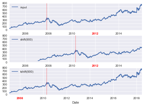
We see here that shift(900) shifts the data by 900 days, pushing
some of it off the end of the graph (and leaving NA values at the other
end), while tshift(900) shifts the index values by 900 days.
A common context for this type of shift is computing differences over time. For example, we use shifted values to compute the one-year return on investment for Google stock over the course of the dataset (Figure 3-9):
In[32]:ROI=100*(goog.tshift(-365)/goog-1)ROI.plot()plt.ylabel('% Return on Investment');
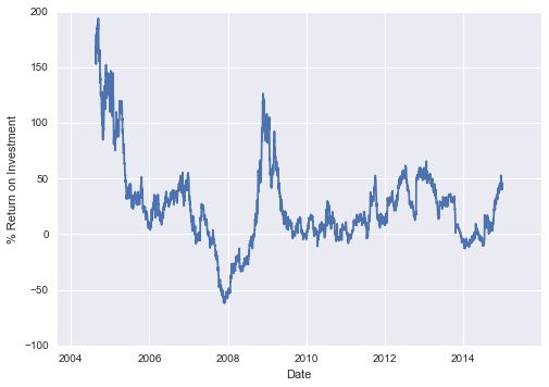
This helps us to see the overall trend in Google stock: thus far, the most profitable times to invest in Google have been (unsurprisingly, in retrospect) shortly after its IPO, and in the middle of the 2009 recession.
Rolling statistics are a third type of time series–specific operation
implemented by Pandas. These can be accomplished via the rolling()
attribute of Series and DataFrame objects, which returns a view similar
to what we saw with the groupby operation (see
“Aggregation and Grouping”).
This rolling view makes available a number of aggregation operations by
default.
For example, here is the one-year centered rolling mean and standard deviation of the Google stock prices (Figure 3-10):
In[33]:rolling=goog.rolling(365,center=True)data=pd.DataFrame({'input':goog,'one-year rolling_mean':rolling.mean(),'one-year rolling_std':rolling.std()})ax=data.plot(style=['-','--',':'])ax.lines[0].set_alpha(0.3)
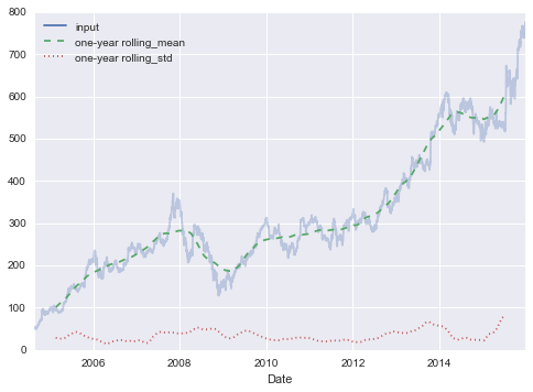
As with groupby operations, the aggregate() and apply() methods can
be used for custom rolling computations.
This section has provided only a brief summary of some of the most essential features of time series tools provided by Pandas; for a more complete discussion, you can refer to the “Time Series/Date” section of the Pandas online documentation.
Another excellent resource is the textbook Python for Data Analysis by Wes McKinney (O’Reilly, 2012). Although it is now a few years old, it is an invaluable resource on the use of Pandas. In particular, this book emphasizes time series tools in the context of business and finance, and focuses much more on particular details of business calendars, time zones, and related topics.
As always, you can also use the IPython help functionality to explore and try further options available to the functions and methods discussed here. I find this often is the best way to learn a new Python tool.
As a more involved example of working with some time series data, let’s take a look at bicycle counts on Seattle’s Fremont Bridge. This data comes from an automated bicycle counter, installed in late 2012, which has inductive sensors on the east and west sidewalks of the bridge. The hourly bicycle counts can be downloaded from http://data.seattle.gov/; here is the direct link to the dataset.
As of summer 2016, the CSV can be downloaded as follows:
In[34]:# !curl -o FremontBridge.csv# https://data.seattle.gov/api/views/65db-xm6k/rows.csv?accessType=DOWNLOAD
Once this dataset is downloaded, we can use Pandas to read the CSV
output into a DataFrame. We will specify that we want the Date as an
index, and we want these dates to be automatically parsed:
In[35]:data=pd.read_csv('FremontBridge.csv',index_col='Date',parse_dates=True)data.head()
Out[35]: Fremont Bridge West Sidewalk \\
Date
2012-10-03 00:00:00 4.0
2012-10-03 01:00:00 4.0
2012-10-03 02:00:00 1.0
2012-10-03 03:00:00 2.0
2012-10-03 04:00:00 6.0
Fremont Bridge East Sidewalk
Date
2012-10-03 00:00:00 9.0
2012-10-03 01:00:00 6.0
2012-10-03 02:00:00 1.0
2012-10-03 03:00:00 3.0
2012-10-03 04:00:00 1.0
For convenience, we’ll further process this dataset by shortening the column names and adding a “Total” column:
In[36]:data.columns=['West','East']data['Total']=data.eval('West + East')
Now let’s take a look at the summary statistics for this data:
In[37]:data.dropna().describe()
Out[37]: West East Total
count 33544.000000 33544.000000 33544.000000
mean 61.726568 53.541706 115.268275
std 83.210813 76.380678 144.773983
min 0.000000 0.000000 0.000000
25% 8.000000 7.000000 16.000000
50% 33.000000 28.000000 64.000000
75% 80.000000 66.000000 151.000000
max 825.000000 717.000000 1186.000000
We can gain some insight into the dataset by visualizing it. Let’s start by plotting the raw data (Figure 3-11):
In[38]:%matplotlibinlineimportseaborn;seaborn.set()
In[39]:data.plot()plt.ylabel('Hourly Bicycle Count');
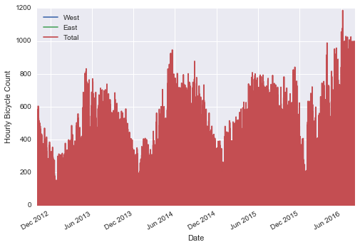
The ~25,000 hourly samples are far too dense for us to make much sense of. We can gain more insight by resampling the data to a coarser grid. Let’s resample by week (Figure 3-12):
In[40]:weekly=data.resample('W').sum()weekly.plot(style=[':','--','-'])plt.ylabel('Weekly bicycle count');
This shows us some interesting seasonal trends: as you might expect, people bicycle more in the summer than in the winter, and even within a particular season the bicycle use varies from week to week (likely dependent on weather; see “In Depth: Linear Regression” where we explore this further).
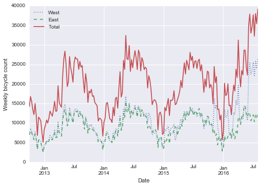
Another way that comes in handy for aggregating the data is to use a rolling mean, utilizing the pd.rolling_mean() function. Here we’ll do a 30-day rolling mean of
our data, making sure to center the window (Figure 3-13):
In[41]:daily=data.resample('D').sum()daily.rolling(30,center=True).sum().plot(style=[':','--','-'])plt.ylabel('mean hourly count');
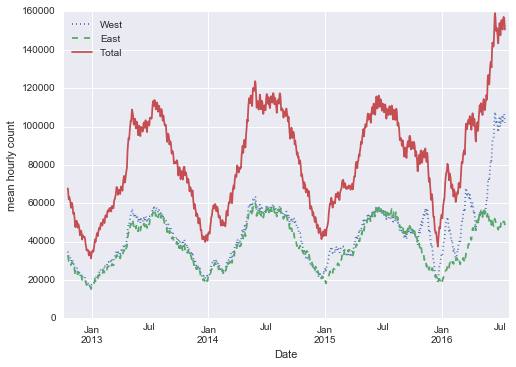
The jaggedness of the result is due to the hard cutoff of the window. We can get a smoother version of a rolling mean using a window function—for example, a Gaussian window. The following code (visualized in Figure 3-14) specifies both the width of the window (we chose 50 days) and the width of the Gaussian within the window (we chose 10 days):
In[42]:daily.rolling(50,center=True,win_type='gaussian').sum(std=10).plot(style=[':','--','-']);
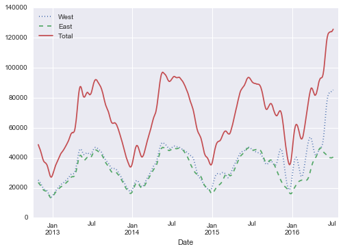
While the smoothed data views in Figure 3-14 are useful to get an idea of the general
trend in the data, they hide much of the interesting structure. For
example, we might want to look at the average traffic as a function of
the time of day. We can do this using the GroupBy functionality
discussed in “Aggregation and Grouping” (Figure 3-15):
In[43]:by_time=data.groupby(data.index.time).mean()hourly_ticks=4*60*60*np.arange(6)by_time.plot(xticks=hourly_ticks,style=[':','--','-']);
The hourly traffic is a strongly bimodal distribution, with peaks around 8:00 in the morning and 5:00 in the evening. This is likely evidence of a strong component of commuter traffic crossing the bridge. This is further evidenced by the differences between the western sidewalk (generally used going toward downtown Seattle), which peaks more strongly in the morning, and the eastern sidewalk (generally used going away from downtown Seattle), which peaks more strongly in the evening.
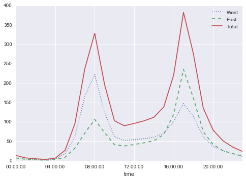
We also might be curious about how things change based on the day of the
week. Again, we can do this with a simple groupby (Figure 3-16):
In[44]:by_weekday=data.groupby(data.index.dayofweek).mean()by_weekday.index=['Mon','Tues','Wed','Thurs','Fri','Sat','Sun']by_weekday.plot(style=[':','--','-']);
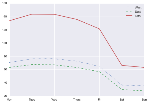
This shows a strong distinction between weekday and weekend totals, with around twice as many average riders crossing the bridge on Monday through Friday than on Saturday and Sunday.
With this in mind, let’s do a compound groupby and look at the hourly
trend on weekdays versus weekends. We’ll start by grouping by both a flag
marking the weekend, and the time of day:
In[45]:weekend=np.where(data.index.weekday<5,'Weekday','Weekend')by_time=data.groupby([weekend,data.index.time]).mean()
Now we’ll use some of the Matplotlib tools described in “Multiple Subplots” to plot two panels side by side (Figure 3-17):
In[46]:importmatplotlib.pyplotaspltfig,ax=plt.subplots(1,2,figsize=(14,5))by_time.ix['Weekday'].plot(ax=ax[0],title='Weekdays',xticks=hourly_ticks,style=[':','--','-'])by_time.ix['Weekend'].plot(ax=ax[1],title='Weekends',xticks=hourly_ticks,style=[':','--','-']);
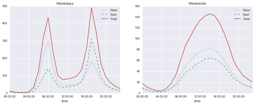
The result is very interesting: we see a bimodal commute pattern during the work week, and a unimodal recreational pattern during the weekends. It would be interesting to dig through this data in more detail, and examine the effect of weather, temperature, time of year, and other factors on people’s commuting patterns; for further discussion, see my blog post “Is Seattle Really Seeing an Uptick In Cycling?”, which uses a subset of this data. We will also revisit this dataset in the context of modeling in “In Depth: Linear Regression”.
As we’ve already seen in previous chapters, the power of the PyData stack is built upon the ability of NumPy and Pandas to push basic operations into C via an intuitive syntax: examples are vectorized/broadcasted operations in NumPy, and grouping-type operations in Pandas. While these abstractions are efficient and effective for many common use cases, they often rely on the creation of temporary intermediate objects, which can cause undue overhead in computational time and memory use.
As of version 0.13 (released January 2014), Pandas includes some
experimental tools that allow you to directly access C-speed operations
without costly allocation of intermediate arrays. These are the eval()
and query() functions, which rely on the
Numexpr package. In this notebook we
will walk through their use and give some rules of thumb about when you
might think about using them.
We’ve seen previously that NumPy and Pandas support fast vectorized operations; for example, when you are adding the elements of two arrays:
In[1]:importnumpyasnprng=np.random.RandomState(42)x=rng.rand(1E6)y=rng.rand(1E6)%timeitx+y
100 loops, best of 3: 3.39 ms per loop
As discussed in “Computation on NumPy Arrays: Universal Functions”, this is much faster than doing the addition via a Python loop or comprehension:
In[2]:%timeitnp.fromiter((xi+yiforxi,yiinzip(x,y)),dtype=x.dtype,count=len(x))
1 loop, best of 3: 266 ms per loop
But this abstraction can become less efficient when you are computing compound expressions. For example, consider the following expression:
In[3]:mask=(x>0.5)&(y<0.5)
Because NumPy evaluates each subexpression, this is roughly equivalent to the following:
In[4]:tmp1=(x>0.5)tmp2=(y<0.5)mask=tmp1&tmp2
In other words, every intermediate step is explicitly allocated in
memory. If the x and y arrays are very large, this can lead to
significant memory and computational overhead. The Numexpr library gives
you the ability to compute this type of compound expression
element by element, without the need to allocate full intermediate
arrays. The Numexpr documentation has
more details, but for the time being it is sufficient to say that the
library accepts a string giving the NumPy-style expression you’d like
to compute:
In[5]:importnumexprmask_numexpr=numexpr.evaluate('(x > 0.5) & (y < 0.5)')np.allclose(mask,mask_numexpr)
Out[5]: True
The benefit here is that Numexpr evaluates the expression in a way that
does not use full-sized temporary arrays, and thus can be much more
efficient than NumPy, especially for large arrays. The Pandas eval()
and query() tools that we will discuss here are conceptually similar, and depend
on the Numexpr package.
The eval() function in Pandas uses string expressions to efficiently
compute operations using DataFrames. For example, consider the following
DataFrames:
In[6]:importpandasaspdnrows,ncols=100000,100rng=np.random.RandomState(42)df1,df2,df3,df4=(pd.DataFrame(rng.rand(nrows,ncols))foriinrange(4))
To compute the sum of all four DataFrames using the typical Pandas
approach, we can just write the sum:
In[7]:%timeitdf1+df2+df3+df4
10 loops, best of 3: 87.1 ms per loop
We can compute the same result via pd.eval by constructing the
expression as a string:
In[8]:%timeitpd.eval('df1 + df2 + df3 + df4')
10 loops, best of 3: 42.2 ms per loop
The eval() version of this expression is about 50% faster (and uses
much less memory), while giving the same result:
In[9]:np.allclose(df1+df2+df3+df4,pd.eval('df1 + df2 + df3 + df4'))
Out[9]: True
As of Pandas v0.16, pd.eval() supports a wide range of operations. To
demonstrate these, we’ll use the following integer DataFrames:
In[10]:df1,df2,df3,df4,df5=(pd.DataFrame(rng.randint(0,1000,(100,3)))foriinrange(5))
pd.eval() supports all arithmetic operators. For example:
In[11]:result1=-df1*df2/(df3+df4)-df5result2=pd.eval('-df1 * df2 / (df3 + df4) - df5')np.allclose(result1,result2)
Out[11]: True
pd.eval() supports all comparison operators, including chained
expressions:
In[12]:result1=(df1<df2)&(df2<=df3)&(df3!=df4)result2=pd.eval('df1 < df2 <= df3 != df4')np.allclose(result1,result2)
Out[12]: True
pd.eval() supports the & and | bitwise operators:
In[13]:result1=(df1<0.5)&(df2<0.5)|(df3<df4)result2=pd.eval('(df1 < 0.5) & (df2 < 0.5) | (df3 < df4)')np.allclose(result1,result2)
Out[13]: True
In addition, it supports the use of the literal and and or in
Boolean expressions:
In[14]:result3=pd.eval('(df1 < 0.5) and (df2 < 0.5) or (df3 < df4)')np.allclose(result1,result3)
Out[14]: True
pd.eval() supports access to object attributes via the obj.attr
syntax, and indexes via the obj[index] syntax:
In[15]:result1=df2.T[0]+df3.iloc[1]result2=pd.eval('df2.T[0] + df3.iloc[1]')np.allclose(result1,result2)
Out[15]: True
Just as Pandas has a top-level pd.eval() function, DataFrames have an
eval() method that works in similar ways. The benefit of the eval()
method is that columns can be referred to by name. We’ll use this
labeled array as an example:
In[16]:df=pd.DataFrame(rng.rand(1000,3),columns=['A','B','C'])df.head()
Out[16]: A B C
0 0.375506 0.406939 0.069938
1 0.069087 0.235615 0.154374
2 0.677945 0.433839 0.652324
3 0.264038 0.808055 0.347197
4 0.589161 0.252418 0.557789
Using pd.eval() as above, we can compute expressions with the three
columns like this:
In[17]:result1=(df['A']+df['B'])/(df['C']-1)result2=pd.eval("(df.A + df.B) / (df.C - 1)")np.allclose(result1,result2)
Out[17]: True
The DataFrame.eval() method allows much more succinct evaluation of
expressions with the columns:
In[18]:result3=df.eval('(A + B) / (C - 1)')np.allclose(result1,result3)
Out[18]: True
Notice here that we treat column names as variables within the evaluated expression, and the result is what we would wish.
In addition to the options just discussed, DataFrame.eval() also
allows assignment to any column. Let’s use the DataFrame from before,
which has columns 'A', 'B', and 'C':
In[19]:df.head()
Out[19]: A B C
0 0.375506 0.406939 0.069938
1 0.069087 0.235615 0.154374
2 0.677945 0.433839 0.652324
3 0.264038 0.808055 0.347197
4 0.589161 0.252418 0.557789
We can use df.eval() to create a new column 'D' and assign to it a
value computed from the other columns:
In[20]:df.eval('D = (A + B) / C',inplace=True)df.head()
Out[20]: A B C D
0 0.375506 0.406939 0.069938 11.187620
1 0.069087 0.235615 0.154374 1.973796
2 0.677945 0.433839 0.652324 1.704344
3 0.264038 0.808055 0.347197 3.087857
4 0.589161 0.252418 0.557789 1.508776
In the same way, any existing column can be modified:
In[21]:df.eval('D = (A - B) / C',inplace=True)df.head()
Out[21]: A B C D
0 0.375506 0.406939 0.069938 -0.449425
1 0.069087 0.235615 0.154374 -1.078728
2 0.677945 0.433839 0.652324 0.374209
3 0.264038 0.808055 0.347197 -1.566886
4 0.589161 0.252418 0.557789 0.603708
The DataFrame.eval() method supports an additional syntax that lets
it work with local Python variables. Consider the following:
In[22]:column_mean=df.mean(1)result1=df['A']+column_meanresult2=df.eval('A + @column_mean')np.allclose(result1,result2)
Out[22]: True
The @ character here marks a variable name rather than a column
name, and lets you efficiently evaluate expressions involving the two
“namespaces”: the namespace of columns, and the namespace of Python
objects. Notice that this @ character is only supported by the
DataFrame.eval() method, not by the pandas.eval() function,
because the pandas.eval() function only has access to the one (Python)
namespace.
The DataFrame has another method based on evaluated strings, called the
query() method. Consider the following:
In[23]:result1=df[(df.A<0.5)&(df.B<0.5)]result2=pd.eval('df[(df.A < 0.5) & (df.B < 0.5)]')np.allclose(result1,result2)
Out[23]: True
As with the example used in our discussion of DataFrame.eval(), this is an expression
involving columns of the DataFrame. It cannot be expressed
using the DataFrame.eval() syntax, however! Instead, for this type of filtering
operation, you can use the query() method:
In[24]:result2=df.query('A < 0.5 and B < 0.5')np.allclose(result1,result2)
Out[24]: True
In addition to being a more efficient computation, compared to the
masking expression this is much easier to read and understand. Note that
the query() method also accepts the @ flag to mark local variables:
In[25]:Cmean=df['C'].mean()result1=df[(df.A<Cmean)&(df.B<Cmean)]result2=df.query('A < @Cmean and B < @Cmean')np.allclose(result1,result2)
Out[25]: True
When considering whether to use these functions, there are two
considerations: computation time and memory use. Memory use is the
most predictable aspect. As already mentioned, every compound expression
involving NumPy arrays or Pandas DataFrames will result in implicit
creation of temporary arrays: For example, this:
In[26]:x=df[(df.A<0.5)&(df.B<0.5)]
is roughly equivalent to this:
In[27]:tmp1=df.A<0.5tmp2=df.B<0.5tmp3=tmp1&tmp2x=df[tmp3]
If the size of the temporary DataFrames is significant compared to your
available system memory (typically several gigabytes), then it’s a good
idea to use an eval() or query() expression. You can check the
approximate size of your array in bytes using this:
In[28]:df.values.nbytes
Out[28]: 32000
On the performance side, eval() can be faster even when you are not
maxing out your system memory. The issue is how your temporary
DataFrames compare to the size of the L1 or L2 CPU cache on your system
(typically a few megabytes in 2016); if they are much bigger, then
eval() can avoid some potentially slow movement of values between the
different memory caches. In practice, I find that the difference in
computation time between the traditional methods and the eval/query
method is usually not significant—if anything, the traditional method
is faster for smaller arrays! The benefit of eval/query is mainly in
the saved memory, and the sometimes cleaner syntax they offer.
We’ve covered most of the details of eval() and query() here; for
more information on these, you can refer to the Pandas documentation. In
particular, different parsers and engines can be specified for running
these queries; for details on this, see the discussion within the
“Enhancing
Performance” section.
In this chapter, we’ve covered many of the basics of using Pandas effectively for data analysis. Still, much has been omitted from our discussion. To learn more about Pandas, I recommend the following resources:
This is the go-to source for complete documentation of the package. While the examples in the documentation tend to be small generated datasets, the description of the options is complete and generally very useful for understanding the use of various functions.
Written by Wes McKinney (the original creator of Pandas), this book contains much more detail on the package than we had room for in this chapter. In particular, he takes a deep dive into tools for time series, which were his bread and butter as a financial consultant. The book also has many entertaining examples of applying Pandas to gain insight from real-world datasets. Keep in mind, though, that the book is now several years old, and the Pandas package has quite a few new features that this book does not cover (but be on the lookout for a new edition in 2017).
Pandas has so many users that any question you have has likely been asked and answered on Stack Overflow. Using Pandas is a case where some Google-Fu is your best friend. Simply go to your favorite search engine and type in the question, problem, or error you’re coming across—more than likely you’ll find your answer on a Stack Overflow page.
From PyCon to SciPy to PyData, many conferences have featured tutorials from Pandas developers and power users. The PyCon tutorials in particular tend to be given by very well-vetted presenters.
My hope is that, by using these resources, combined with the walk-through given in this chapter, you’ll be poised to use Pandas to tackle any data analysis problem you come across!
1 You can learn more about sigma-clipping operations in a book I coauthored with Željko Ivezić, Andrew J. Connolly, and Alexander Gray: Statistics, Data Mining, and Machine Learning in Astronomy: A Practical Python Guide for the Analysis of Survey Data (Princeton University Press, 2014).
We’ll now take an in-depth look at the Matplotlib tool for visualization in Python. Matplotlib is a multiplatform data visualization library built on NumPy arrays, and designed to work with the broader SciPy stack. It was conceived by John Hunter in 2002, originally as a patch to IPython for enabling interactive MATLAB-style plotting via gnuplot from the IPython command line. IPython’s creator, Fernando Perez, was at the time scrambling to finish his PhD, and let John know he wouldn’t have time to review the patch for several months. John took this as a cue to set out on his own, and the Matplotlib package was born, with version 0.1 released in 2003. It received an early boost when it was adopted as the plotting package of choice of the Space Telescope Science Institute (the folks behind the Hubble Telescope), which financially supported Matplotlib’s development and greatly expanded its capabilities.
One of Matplotlib’s most important features is its ability to play well with many operating systems and graphics backends. Matplotlib supports dozens of backends and output types, which means you can count on it to work regardless of which operating system you are using or which output format you wish. This cross-platform, everything-to-everyone approach has been one of the great strengths of Matplotlib. It has led to a large userbase, which in turn has led to an active developer base and Matplotlib’s powerful tools and ubiquity within the scientific Python world.
In recent years, however, the interface and style of Matplotlib have begun to show their age. Newer tools like ggplot and ggvis in the R language, along with web visualization toolkits based on D3js and HTML5 canvas, often make Matplotlib feel clunky and old-fashioned. Still, I’m of the opinion that we cannot ignore Matplotlib’s strength as a well-tested, cross-platform graphics engine. Recent Matplotlib versions make it relatively easy to set new global plotting styles (see “Customizing Matplotlib: Configurations and Stylesheets”), and people have been developing new packages that build on its powerful internals to drive Matplotlib via cleaner, more modern APIs—for example, Seaborn (discussed in “Visualization with Seaborn”), ggplot, HoloViews, Altair, and even Pandas itself can be used as wrappers around Matplotlib’s API. Even with wrappers like these, it is still often useful to dive into Matplotlib’s syntax to adjust the final plot output. For this reason, I believe that Matplotlib itself will remain a vital piece of the data visualization stack, even if new tools mean the community gradually moves away from using the Matplotlib API directly.
Before we dive into the details of creating visualizations with Matplotlib, there are a few useful things you should know about using the package.
Just as we use the np shorthand for NumPy and the pd shorthand for
Pandas, we will use some standard shorthands for Matplotlib imports:
In[1]:importmatplotlibasmplimportmatplotlib.pyplotasplt
The plt interface is what we will use most often, as we’ll see
throughout this chapter.
We will use the plt.style directive to choose
appropriate aesthetic styles for our figures. Here we will set the
classic style, which ensures that the plots we create use the classic
Matplotlib style:
In[2]:plt.style.use('classic')
Throughout this section, we will adjust this style as needed. Note that the stylesheets used here are supported as of Matplotlib version 1.5; if you are using an earlier version of Matplotlib, only the default style is available. For more information on stylesheets, see “Customizing Matplotlib: Configurations and Stylesheets”.
A visualization you can’t see won’t be of much use, but just how you view your Matplotlib plots depends on the context. The best use of Matplotlib differs depending on how you are using it; roughly, the three applicable contexts are using Matplotlib in a script, in an IPython terminal, or in an IPython notebook.
If you are using Matplotlib from within a script, the function
plt.show() is your friend. plt.show() starts an event loop, looks
for all currently active figure objects, and opens one or more
interactive windows that display your figure or figures.
So, for example, you may have a file called myplot.py containing the following:
# ------- file: myplot.py ------importmatplotlib.pyplotaspltimportnumpyasnpx=np.linspace(0,10,100)plt.plot(x,np.sin(x))plt.plot(x,np.cos(x))plt.show()
You can then run this script from the command-line prompt, which will result in a window opening with your figure displayed:
$ python myplot.py
The plt.show() command does a lot under the hood, as it must interact with
your system’s interactive graphical backend. The details of this
operation can vary greatly from system to system and even installation
to installation, but Matplotlib does its best to hide all these details
from you.
One thing to be aware of: the plt.show() command should be used only
once per Python session, and is most often seen at the very end of the
script. Multiple show() commands can lead to unpredictable
backend-dependent behavior, and should mostly be avoided.
It can be very convenient to use Matplotlib interactively within an
IPython shell (see
Chapter 1). IPython is built to work well with Matplotlib if you specify
Matplotlib mode. To enable this mode, you can use the %matplotlib
magic command after starting ipython:
In[1]:%matplotlibUsingmatplotlibbackend:TkAggIn[2]:importmatplotlib.pyplotasplt
At this point, any plt plot command will cause a figure window to
open, and further commands can be run to update the plot. Some changes
(such as modifying properties of lines that are already drawn) will not
draw automatically; to force an update, use plt.draw(). Using
plt.show() in Matplotlib mode is not required.
The IPython notebook is a browser-based interactive data analysis tool that can combine narrative, code, graphics, HTML elements, and much more into a single executable document (see Chapter 1).
Plotting interactively within an IPython notebook can be done with the
%matplotlib command, and works in a similar way to the IPython shell.
In the IPython notebook, you also have the option of embedding graphics
directly in the notebook, with two possible options:
%matplotlib notebook will lead to interactive plots embedded
within the notebook
%matplotlib inline will lead to static images of your plot
embedded in the notebook
For this book, we will generally opt for %matplotlib inline:
In[3]:%matplotlibinline
After you run this command (it needs to be done only once per kernel/session), any cell within the notebook that creates a plot will embed a PNG image of the resulting graphic (Figure 4-1):
In[4]:importnumpyasnpx=np.linspace(0,10,100)fig=plt.figure()plt.plot(x,np.sin(x),'-')plt.plot(x,np.cos(x),'--');
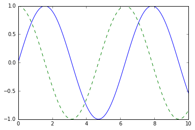
One nice feature of Matplotlib is the ability to save figures in a wide
variety of formats. You can save a figure using the savefig()
command. For example, to save the previous figure as a PNG file, you can
run this:
In[5]:fig.savefig('my_figure.png')
We now have a file called my_figure.png in the current working directory:
In[6]:!ls-lhmy_figure.png
-rw-r--r-- 1 jakevdp staff 16K Aug 11 10:59 my_figure.png
To confirm that it contains what we think it contains, let’s use the
IPython Image object to display the contents of this file (Figure 4-2):
In[7]:fromIPython.displayimportImageImage('my_figure.png')
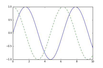
In savefig(), the file format is inferred from the extension of the
given filename. Depending on what backends you have installed, many
different file formats are available. You can find the list of supported file types for your system by using the following method of the figure
canvas object:
In[8]:fig.canvas.get_supported_filetypes()
Out[8]: {'eps': 'Encapsulated Postscript',
'jpeg': 'Joint Photographic Experts Group',
'jpg': 'Joint Photographic Experts Group',
'pdf': 'Portable Document Format',
'pgf': 'PGF code for LaTeX',
'png': 'Portable Network Graphics',
'ps': 'Postscript',
'raw': 'Raw RGBA bitmap',
'rgba': 'Raw RGBA bitmap',
'svg': 'Scalable Vector Graphics',
'svgz': 'Scalable Vector Graphics',
'tif': 'Tagged Image File Format',
'tiff': 'Tagged Image File Format'}
Note that when saving your figure, it’s not necessary to use plt.show() or
related commands discussed earlier.
A potentially confusing feature of Matplotlib is its dual interfaces: a convenient MATLAB-style state-based interface, and a more powerful object-oriented interface. We’ll quickly highlight the differences between the two here.
Matplotlib was originally written as a Python alternative for MATLAB
users, and much of its syntax reflects that fact. The MATLAB-style tools
are contained in the pyplot (plt) interface. For example, the
following code will probably look quite familiar to MATLAB users (Figure 4-3):
In[9]:plt.figure()# create a plot figure# create the first of two panels and set current axisplt.subplot(2,1,1)# (rows, columns, panel number)plt.plot(x,np.sin(x))# create the second panel and set current axisplt.subplot(2,1,2)plt.plot(x,np.cos(x));

It’s important to note that this interface is stateful: it keeps track of the
“current” figure and axes, which are where all plt commands are
applied. You can get a reference to these using the plt.gcf() (get
current figure) and plt.gca() (get current axes) routines.
While this stateful interface is fast and convenient for simple plots, it is easy to run into problems. For example, once the second panel is created, how can we go back and add something to the first? This is possible within the MATLAB-style interface, but a bit clunky. Fortunately, there is a better way.
The object-oriented interface is available for these more complicated
situations, and for when you want more control over your figure. Rather
than depending on some notion of an “active” figure or axes, in the
object-oriented interface the plotting functions are methods of
explicit Figure and Axes objects. To re-create the previous plot using
this style of plotting, you might do the following (Figure 4-4):
In[10]:# First create a grid of plots# ax will be an array of two Axes objectsfig,ax=plt.subplots(2)# Call plot() method on the appropriate objectax[0].plot(x,np.sin(x))ax[1].plot(x,np.cos(x));
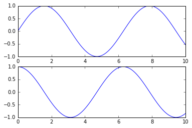
For more simple plots, the choice of which style to use is largely a matter of preference, but the object-oriented approach can become a necessity as plots become
more complicated. Throughout this chapter, we will switch between the
MATLAB-style and object-oriented interfaces, depending on what is most
convenient. In most cases, the difference is as small as switching
plt.plot() to ax.plot(), but there are a few gotchas that we will
highlight as they come up in the following sections.
Perhaps the simplest of all plots is the visualization of a single
function  . Here we will take a first look at
creating a simple plot of this type. As with all the following sections,
we’ll start by setting up the notebook for plotting and importing the functions we will use:
. Here we will take a first look at
creating a simple plot of this type. As with all the following sections,
we’ll start by setting up the notebook for plotting and importing the functions we will use:
In[1]:%matplotlibinlineimportmatplotlib.pyplotaspltplt.style.use('seaborn-whitegrid')importnumpyasnp
For all Matplotlib plots, we start by creating a figure and an axes. In their simplest form, a figure and axes can be created as follows (Figure 4-5):
In[2]:fig=plt.figure()ax=plt.axes()
In Matplotlib, the figure (an instance of the class plt.Figure) can
be thought of as a single container that contains all the objects
representing axes, graphics, text, and labels. The axes (an instance
of the class plt.Axes) is what we see above: a bounding box with ticks
and labels, which will eventually contain the plot elements that make up
our visualization. Throughout this book, we’ll commonly use the variable
name fig to refer to a figure instance, and ax to refer to an axes
instance or group of axes instances.
Once we have created an axes, we can use the ax.plot function to plot
some data. Let’s start with a simple sinusoid (Figure 4-6):
In[3]:fig=plt.figure()ax=plt.axes()x=np.linspace(0,10,1000)ax.plot(x,np.sin(x));

Alternatively, we can use the pylab interface and let the figure and axes be created for us in the background (Figure 4-7; see “Two Interfaces for the Price of One” for a discussion of these two interfaces):
In[4]:plt.plot(x,np.sin(x));

If we want to create a single figure with multiple lines, we can simply
call the plot function multiple times (Figure 4-8):
In[5]:plt.plot(x,np.sin(x))plt.plot(x,np.cos(x));
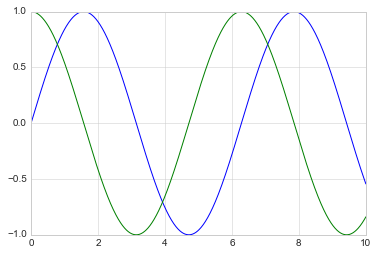
That’s all there is to plotting simple functions in Matplotlib! We’ll now dive into some more details about how to control the appearance of the axes and lines.
The first adjustment you might wish to make to a plot is to control the
line colors and styles. The plt.plot() function takes additional
arguments that can be used to specify these. To adjust the color, you
can use the color keyword, which accepts a string argument
representing virtually any imaginable color. The color can be specified
in a variety of ways (Figure 4-9):
In[6]:plt.plot(x,np.sin(x-0),color='blue')# specify color by nameplt.plot(x,np.sin(x-1),color='g')# short color code (rgbcmyk)plt.plot(x,np.sin(x-2),color='0.75')# Grayscale between 0 and 1plt.plot(x,np.sin(x-3),color='#FFDD44')# Hex code (RRGGBB from 00 to FF)plt.plot(x,np.sin(x-4),color=(1.0,0.2,0.3))# RGB tuple, values 0 and 1plt.plot(x,np.sin(x-5),color='chartreuse');# all HTML color names supported
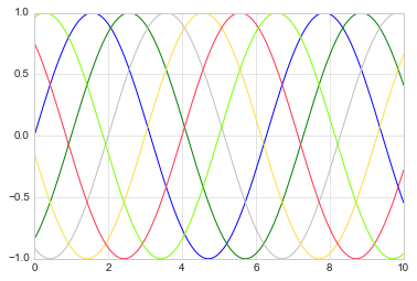
If no color is specified, Matplotlib will automatically cycle through a set of default colors for multiple lines.
Similarly, you can adjust the line style using the linestyle keyword (Figure 4-10):
In[7]:plt.plot(x,x+0,linestyle='solid')plt.plot(x,x+1,linestyle='dashed')plt.plot(x,x+2,linestyle='dashdot')plt.plot(x,x+3,linestyle='dotted');# For short, you can use the following codes:plt.plot(x,x+4,linestyle='-')# solidplt.plot(x,x+5,linestyle='--')# dashedplt.plot(x,x+6,linestyle='-.')# dashdotplt.plot(x,x+7,linestyle=':');# dotted
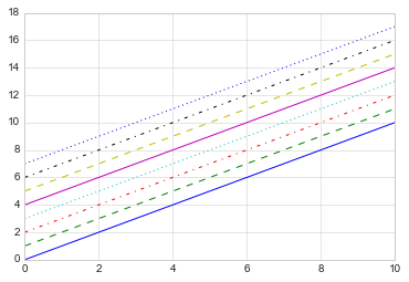
If you would like to be extremely terse, these linestyle and color
codes can be combined into a single nonkeyword argument to the
plt.plot() function (Figure 4-11):
In[8]:plt.plot(x,x+0,'-g')# solid greenplt.plot(x,x+1,'--c')# dashed cyanplt.plot(x,x+2,'-.k')# dashdot blackplt.plot(x,x+3,':r');# dotted red
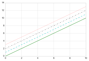
These single-character color codes reflect the standard abbreviations in the RGB (Red/Green/Blue) and CMYK (Cyan/Magenta/Yellow/blacK) color systems, commonly used for digital color graphics.
There are many other keyword arguments that can be used to fine-tune the
appearance of the plot; for more details, I’d suggest viewing the
docstring of the plt.plot() function using IPython’s help tools (see
“Help and Documentation in IPython”).
Matplotlib does a decent job of choosing default axes limits for your
plot, but sometimes it’s nice to have finer control. The most basic way
to adjust axis limits is to use the plt.xlim() and plt.ylim()
methods (Figure 4-12):
In[9]:plt.plot(x,np.sin(x))plt.xlim(-1,11)plt.ylim(-1.5,1.5);
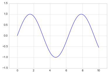
If for some reason you’d like either axis to be displayed in reverse, you can simply reverse the order of the arguments (Figure 4-13):
In[10]:plt.plot(x,np.sin(x))plt.xlim(10,0)plt.ylim(1.2,-1.2);
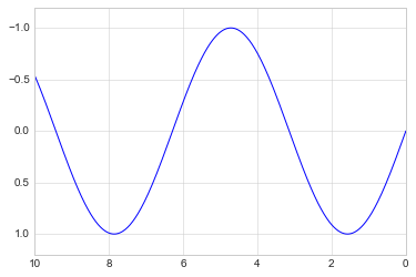
A useful related method is plt.axis() (note here the potential
confusion between axes with an e, and axis with an i). The
plt.axis() method allows you to set the x and y limits with a single
call, by passing a list that specifies [xmin, xmax, ymin, ymax] (Figure 4-14):
In[11]:plt.plot(x,np.sin(x))plt.axis([-1,11,-1.5,1.5]);

The plt.axis() method goes even beyond this, allowing you to do things
like automatically tighten the bounds around the current plot (Figure 4-15):
In[12]:plt.plot(x,np.sin(x))plt.axis('tight');
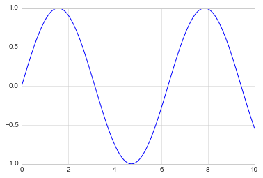
It allows even higher-level specifications, such as ensuring an equal
aspect ratio so that on your screen, one unit in x is equal to one unit
in y (Figure 4-16):
In[13]:plt.plot(x,np.sin(x))plt.axis('equal');
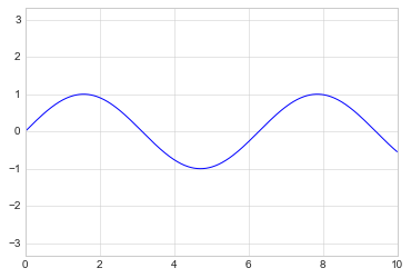
For more information on axis limits and the other capabilities of the
plt.axis() method, refer to the plt.axis() docstring.
As the last piece of this section, we’ll briefly look at the labeling of plots: titles, axis labels, and simple legends.
Titles and axis labels are the simplest such labels—there are methods that can be used to quickly set them (Figure 4-17):
In[14]:plt.plot(x,np.sin(x))plt.title("A Sine Curve")plt.xlabel("x")plt.ylabel("sin(x)");
You can adjust the position, size, and style of these labels using optional arguments to the function. For more information, see the Matplotlib documentation and the docstrings of each of these functions.
When multiple lines are being shown within a single axes, it can be
useful to create a plot legend that labels each line type. Again,
Matplotlib has a built-in way of quickly creating such a legend. It is
done via the (you guessed it) plt.legend() method. Though there are
several valid ways of using this, I find it easiest to specify the label
of each line using the label keyword of the plot function (Figure 4-18):
In[15]:plt.plot(x,np.sin(x),'-g',label='sin(x)')plt.plot(x,np.cos(x),':b',label='cos(x)')plt.axis('equal')plt.legend();
As you can see, the plt.legend() function keeps track of the line
style and color, and matches these with the correct label. More
information on specifying and formatting plot legends can be found in
the plt.legend() docstring; additionally, we will cover some more
advanced legend options in
“Customizing Plot Legends”.
Another commonly used plot type is the simple scatter plot, a close cousin of the line plot. Instead of points being joined by line segments, here the points are represented individually with a dot, circle, or other shape. We’ll start by setting up the notebook for plotting and importing the functions we will use:
In[1]:%matplotlibinlineimportmatplotlib.pyplotaspltplt.style.use('seaborn-whitegrid')importnumpyasnp
In the previous section, we looked at plt.plot/ax.plot to produce line
plots. It turns out that this same function can produce scatter plots as
well (Figure 4-20):
In[2]:x=np.linspace(0,10,30)y=np.sin(x)plt.plot(x,y,'o',color='black');
The third argument in the function call is a character that represents
the type of symbol used for the plotting. Just as you can specify options such as '-' and '--' to control the line style, the marker style has its own set
of short string codes. The full list of available symbols can be seen in
the documentation of plt.plot, or in Matplotlib’s online
documentation. Most of the possibilities are fairly intuitive, and we’ll
show a number of the more common ones here (Figure 4-21):
In[3]:rng=np.random.RandomState(0)formarkerin['o','.',',','x','+','v','^','<','>','s','d']:plt.plot(rng.rand(5),rng.rand(5),marker,label="marker='{0}'".format(marker))plt.legend(numpoints=1)plt.xlim(0,1.8);
For even more possibilities, these character codes can be used together with line and color codes to plot points along with a line connecting them (Figure 4-22):
In[4]:plt.plot(x,y,'-ok');# line (-), circle marker (o), black (k)
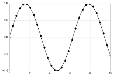
Additional keyword arguments to plt.plot specify a wide range of
properties of the lines and markers (Figure 4-23):
In[5]:plt.plot(x,y,'-p',color='gray',markersize=15,linewidth=4,markerfacecolor='white',markeredgecolor='gray',markeredgewidth=2)plt.ylim(-1.2,1.2);
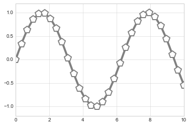
This type of flexibility in the plt.plot function allows for a wide
variety of possible visualization options. For a full description of the
options available, refer to the plt.plot documentation.
A second, more powerful method of creating scatter plots is the
plt.scatter function, which can be used very similarly to the
plt.plot function (Figure 4-24):
In[6]:plt.scatter(x,y,marker='o');
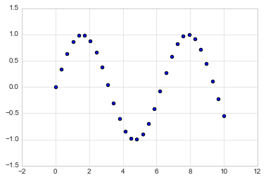
The primary difference of plt.scatter from plt.plot is that it can
be used to create scatter plots where the properties of each individual
point (size, face color, edge color, etc.) can be individually
controlled or mapped to data.
Let’s show this by creating a random scatter plot with points of many
colors and sizes. In order to better see the overlapping results, we’ll
also use the alpha keyword to adjust the transparency level (Figure 4-25):
In[7]:rng=np.random.RandomState(0)x=rng.randn(100)y=rng.randn(100)colors=rng.rand(100)sizes=1000*rng.rand(100)plt.scatter(x,y,c=colors,s=sizes,alpha=0.3,cmap='viridis')plt.colorbar();# show color scale
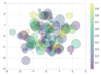
Notice that the color argument is
automatically mapped to a color scale (shown here by the colorbar()
command), and the size argument is given in pixels. In this way, the
color and size of points can be used to convey information in the
visualization, in order to illustrate multidimensional data.
For example, we might use the Iris data from Scikit-Learn, where each sample is one of three types of flowers that has had the size of its petals and sepals carefully measured (Figure 4-26):
In[8]:fromsklearn.datasetsimportload_irisiris=load_iris()features=iris.data.Tplt.scatter(features[0],features[1],alpha=0.2,s=100*features[3],c=iris.target,cmap='viridis')plt.xlabel(iris.feature_names[0])plt.ylabel(iris.feature_names[1]);
We can see that this scatter plot has given us the ability to simultaneously explore four different dimensions of the data: the (x, y) location of each point corresponds to the sepal length and width, the size of the point is related to the petal width, and the color is related to the particular species of flower. Multicolor and multifeature scatter plots like this can be useful for both exploration and presentation of data.
Aside from the different features available in plt.plot and
plt.scatter, why might you choose to use one over the other? While it
doesn’t matter as much for small amounts of data, as datasets get larger
than a few thousand points, plt.plot can be noticeably more efficient
than plt.scatter. The reason is that plt.scatter has the capability
to render a different size and/or color for each point, so the renderer
must do the extra work of constructing each point individually. In
plt.plot, on the other hand, the points are always essentially clones
of each other, so the work of determining the appearance of the points
is done only once for the entire set of data. For large datasets, the
difference between these two can lead to vastly different performance,
and for this reason, plt.plot should be preferred over plt.scatter
for large datasets.
For any scientific measurement, accurate accounting for errors is nearly as important, if not more important, than accurate reporting of the number itself. For example, imagine that I am using some astrophysical observations to estimate the Hubble Constant, the local measurement of the expansion rate of the universe. I know that the current literature suggests a value of around 71 (km/s)/Mpc, and I measure a value of 74 (km/s)/Mpc with my method. Are the values consistent? The only correct answer, given this information, is this: there is no way to know.
Suppose I augment this information with reported uncertainties: the
current literature suggests a value of around 71  2.5
(km/s)/Mpc, and my method has measured a value of 74
2.5
(km/s)/Mpc, and my method has measured a value of 74  5
(km/s)/Mpc. Now are the values consistent? That is a question that can
be quantitatively answered.
5
(km/s)/Mpc. Now are the values consistent? That is a question that can
be quantitatively answered.
In visualization of data and results, showing these errors effectively can make a plot convey much more complete information.
A basic errorbar can be created with a single Matplotlib function call (Figure 4-27):
In[1]:%matplotlibinlineimportmatplotlib.pyplotaspltplt.style.use('seaborn-whitegrid')importnumpyasnp
In[2]:x=np.linspace(0,10,50)dy=0.8y=np.sin(x)+dy*np.random.randn(50)plt.errorbar(x,y,yerr=dy,fmt='.k');
Here the fmt is a format code controlling the appearance of lines and
points, and has the same syntax as the shorthand used in plt.plot,
outlined in “Simple Line Plots” and
“Simple Scatter Plots”.
In addition to these basic options, the errorbar function has many
options to fine-tune the outputs. Using these additional options you can
easily customize the aesthetics of your errorbar plot. I often find it
helpful, especially in crowded plots, to make the errorbars lighter than
the points themselves (Figure 4-28):
In[3]:plt.errorbar(x,y,yerr=dy,fmt='o',color='black',ecolor='lightgray',elinewidth=3,capsize=0);
In addition to these options, you can also specify horizontal errorbars
(xerr), one-sided errorbars, and many other variants. For more
information on the options available, refer to the docstring of
plt.errorbar.
In some situations it is desirable to show errorbars on continuous
quantities. Though Matplotlib does not have a built-in convenience
routine for this type of application, it’s relatively easy to combine
primitives like plt.plot and plt.fill_between for a useful result.
Here we’ll perform a simple Gaussian process regression (GPR), using the Scikit-Learn API (see “Introducing Scikit-Learn” for details). This is a method of fitting a very flexible nonparametric function to data with a continuous measure of the uncertainty. We won’t delve into the details of Gaussian process regression at this point, but will focus instead on how you might visualize such a continuous error measurement:
In[4]:fromsklearn.gaussian_processimportGaussianProcess# define the model and draw some datamodel=lambdax:x*np.sin(x)xdata=np.array([1,3,5,6,8])ydata=model(xdata)# Compute the Gaussian process fitgp=GaussianProcess(corr='cubic',theta0=1e-2,thetaL=1e-4,thetaU=1E-1,random_start=100)gp.fit(xdata[:,np.newaxis],ydata)xfit=np.linspace(0,10,1000)yfit,MSE=gp.predict(xfit[:,np.newaxis],eval_MSE=True)dyfit=2*np.sqrt(MSE)# 2*sigma ~ 95% confidence region
We now have xfit, yfit, and dyfit, which sample the continuous fit
to our data. We could pass these to the plt.errorbar function as
above, but we don’t really want to plot 1,000 points with 1,000 errorbars.
Instead, we can use the plt.fill_between function with a light color
to visualize this continuous error (Figure 4-29):
In[5]:# Visualize the resultplt.plot(xdata,ydata,'or')plt.plot(xfit,yfit,'-',color='gray')plt.fill_between(xfit,yfit-dyfit,yfit+dyfit,color='gray',alpha=0.2)plt.xlim(0,10);
Note what we’ve done here with the fill_between function: we pass an x
value, then the lower y-bound, then the upper y-bound, and the result is
that the area between these regions is filled.
The resulting figure gives a very intuitive view into what the Gaussian process regression algorithm is doing: in regions near a measured data point, the model is strongly constrained and this is reflected in the small model errors. In regions far from a measured data point, the model is not strongly constrained, and the model errors increase.
For more information on the options available in plt.fill_between()
(and the closely related plt.fill() function), see the function
docstring or the Matplotlib documentation.
Finally, if this seems a bit too low level for your taste, refer to “Visualization with Seaborn”, where we discuss the Seaborn package, which has a more streamlined API for visualizing this type of continuous errorbar.
Sometimes it is useful to display three-dimensional data in
two dimensions using contours or color-coded regions. There are three
Matplotlib functions that can be helpful for this task: plt.contour
for contour plots, plt.contourf for filled contour plots, and
plt.imshow for showing images. This section looks at several examples of using these. We’ll start by setting up the notebook for plotting and importing the functions we will use:
In[1]:%matplotlibinlineimportmatplotlib.pyplotaspltplt.style.use('seaborn-white')importnumpyasnp
We’ll start by demonstrating a contour plot using a function
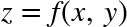 , using the following particular choice for
 (we’ve seen this before in
“Computation on Arrays: Broadcasting”, when we used it as a motivating example for array
broadcasting):
(we’ve seen this before in
“Computation on Arrays: Broadcasting”, when we used it as a motivating example for array
broadcasting):
In[2]:deff(x,y):returnnp.sin(x)**10+np.cos(10+y*x)*np.cos(x)
A contour plot can be created with the plt.contour function. It takes
three arguments: a grid of x values, a grid of y values, and a grid of z
values. The x and y values represent positions on the plot, and the z
values will be represented by the contour levels. Perhaps the most
straightforward way to prepare such data is to use the np.meshgrid
function, which builds two-dimensional grids from one-dimensional arrays:
In[3]:x=np.linspace(0,5,50)y=np.linspace(0,5,40)X,Y=np.meshgrid(x,y)Z=f(X,Y)
Now let’s look at this with a standard line-only contour plot (Figure 4-30):
In[4]:plt.contour(X,Y,Z,colors='black');
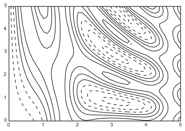
Notice that by default when a single color is used, negative values are
represented by dashed lines, and positive values by solid lines.
Alternatively, you can color-code the lines by specifying a colormap
with the cmap argument. Here, we’ll also specify that we want more
lines to be drawn—20 equally spaced intervals within the data range (Figure 4-31):
In[5]:plt.contour(X,Y,Z,20,cmap='RdGy');
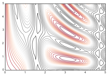
Here we chose the RdGy (short for Red-Gray) colormap, which is a good
choice for centered data. Matplotlib has a wide range of colormaps
available, which you can easily browse in IPython by doing a
tab completion on the plt.cm module:
plt.cm.<TAB>
Our plot is looking nicer, but the spaces between the lines may be
a bit distracting. We can change this by switching to a filled contour
plot using the plt.contourf() function (notice the f at the end),
which uses largely the same syntax as plt.contour().
Additionally, we’ll add a plt.colorbar() command, which automatically
creates an additional axis with labeled color information for the plot (Figure 4-32):
In[6]:plt.contourf(X,Y,Z,20,cmap='RdGy')plt.colorbar();
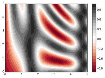
The colorbar makes it clear that the black regions are “peaks,” while the red regions are “valleys.”
One potential issue with this plot is that it is a bit “splotchy.” That
is, the color steps are discrete rather than continuous, which is not
always what is desired. You could remedy this by setting the number of
contours to a very high number, but this results in a rather inefficient
plot: Matplotlib must render a new polygon for each step in the level. A
better way to handle this is to use the plt.imshow() function, which
interprets a two-dimensional grid of data as an image.
Figure 4-33 shows the result of the following code:
In[7]:plt.imshow(Z,extent=[0,5,0,5],origin='lower',cmap='RdGy')plt.colorbar()plt.axis(aspect='image');
There are a few potential gotchas with imshow(), however:
plt.imshow() doesn’t accept an x and y grid, so you must manually
specify the extent [xmin, xmax, ymin, ymax] of the image on the plot.
plt.imshow() by default follows the standard image array definition
where the origin is in the upper left, not in the lower left as in most
contour plots. This must be changed when showing gridded data.
plt.imshow() will automatically adjust the axis aspect ratio to
match the input data; you can change this by setting, for example,
plt.axis(aspect='image') to make x and y units match.
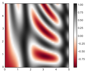
Finally, it can sometimes be useful to combine contour plots and image
plots. For example, to create the effect shown in Figure 4-34, we’ll use a partially
transparent background image (with transparency set via the alpha
parameter) and over-plot contours with labels on the contours themselves
(using the plt.clabel() function):
In[8]:contours=plt.contour(X,Y,Z,3,colors='black')plt.clabel(contours,inline=True,fontsize=8)plt.imshow(Z,extent=[0,5,0,5],origin='lower',cmap='RdGy',alpha=0.5)plt.colorbar();
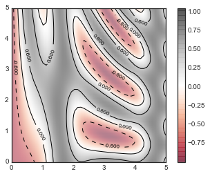
The combination of these three functions—plt.contour, plt.contourf,
and plt.imshow—gives nearly limitless possibilities for displaying
this sort of three-dimensional data within a two-dimensional plot. For
more information on the options available in these functions, refer to
their docstrings. If you are interested in three-dimensional
visualizations of this type of data, see
“Three-Dimensional Plotting in Matplotlib”.
A simple histogram can be a great first step in understanding a dataset. Earlier, we saw a preview of Matplotlib’s histogram function (see “Comparisons, Masks, and Boolean Logic”), which creates a basic histogram in one line, once the normal boilerplate imports are done (Figure 4-35):
In[1]:%matplotlibinlineimportnumpyasnpimportmatplotlib.pyplotaspltplt.style.use('seaborn-white')data=np.random.randn(1000)
In[2]:plt.hist(data);
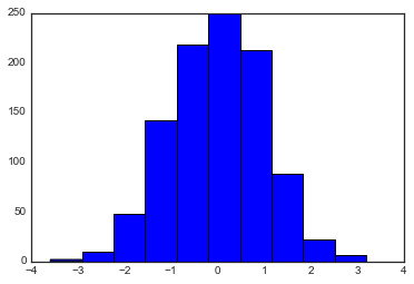
The hist() function has many options to tune both the calculation and
the display; here’s an example of a more customized histogram (Figure 4-36):
In[3]:plt.hist(data,bins=30,normed=True,alpha=0.5,histtype='stepfilled',color='steelblue',edgecolor='none');
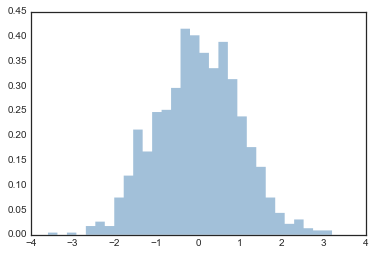
The plt.hist docstring has more information on other customization
options available. I find this combination of
histtype='stepfilled' along with some transparency alpha to be very
useful when comparing histograms of several distributions (Figure 4-37):
In[4]:x1=np.random.normal(0,0.8,1000)x2=np.random.normal(-2,1,1000)x3=np.random.normal(3,2,1000)kwargs=dict(histtype='stepfilled',alpha=0.3,normed=True,bins=40)plt.hist(x1,**kwargs)plt.hist(x2,**kwargs)plt.hist(x3,**kwargs);
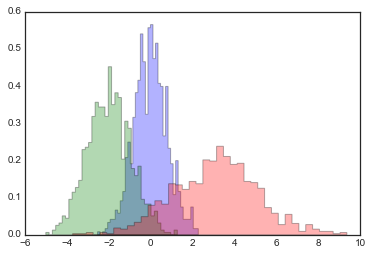
If you would like to simply compute the histogram (that is, count the
number of points in a given bin) and not display it, the
np.histogram() function is available:
In[5]:counts,bin_edges=np.histogram(data,bins=5)(counts)
[ 12 190 468 301 29]
Just as we create histograms in one dimension by dividing the
number line into bins, we can also create histograms in two dimensions
by dividing points among two-dimensional bins. We’ll take a brief look
at several ways to do this here. We’ll start by defining some data—an
x and y array drawn from a multivariate Gaussian distribution:
In[6]:mean=[0,0]cov=[[1,1],[1,2]]x,y=np.random.multivariate_normal(mean,cov,10000).T
One straightforward way to plot a two-dimensional histogram is to use Matplotlib’s
plt.hist2d function (Figure 4-38):
In[12]:plt.hist2d(x,y,bins=30,cmap='Blues')cb=plt.colorbar()cb.set_label('counts in bin')
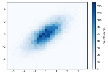
Just as with plt.hist, plt.hist2d has a number of extra options to
fine-tune the plot and the binning, which are nicely outlined in the function
docstring. Further, just as plt.hist has a counterpart in np.histogram,
plt.hist2d has a counterpart in np.histogram2d, which can be used as
follows:
In[8]:counts,xedges,yedges=np.histogram2d(x,y,bins=30)
For the generalization of this histogram binning in dimensions higher
than two, see the np.histogramdd function.
The two-dimensional histogram creates a tessellation of squares across
the axes. Another natural shape for such a tessellation is the regular
hexagon. For this purpose, Matplotlib provides the plt.hexbin routine,
which represents a two-dimensional dataset binned within a grid of
hexagons (Figure 4-39):
In[9]:plt.hexbin(x,y,gridsize=30,cmap='Blues')cb=plt.colorbar(label='count in bin')

plt.hexbin has a number of interesting options, including the ability
to specify weights for each point, and to change the output in each bin
to any NumPy aggregate (mean of weights, standard deviation of weights,
etc.).
Another common method of evaluating densities in multiple dimensions is
kernel density estimation (KDE). This will be discussed more fully in
“In-Depth: Kernel Density Estimation”, but for now we’ll simply mention that KDE can be thought of
as a way to “smear out” the points in space and add up the result to
obtain a smooth function. One extremely quick and simple KDE
implementation exists in the scipy.stats package. Here is a quick
example of using the KDE on this data (Figure 4-40):
In[10]:fromscipy.statsimportgaussian_kde# fit an array of size [Ndim, Nsamples]data=np.vstack([x,y])kde=gaussian_kde(data)# evaluate on a regular gridxgrid=np.linspace(-3.5,3.5,40)ygrid=np.linspace(-6,6,40)Xgrid,Ygrid=np.meshgrid(xgrid,ygrid)Z=kde.evaluate(np.vstack([Xgrid.ravel(),Ygrid.ravel()]))# Plot the result as an imageplt.imshow(Z.reshape(Xgrid.shape),origin='lower',aspect='auto',extent=[-3.5,3.5,-6,6],cmap='Blues')cb=plt.colorbar()cb.set_label("density")
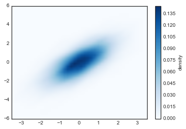
KDE has a smoothing length that effectively slides the knob between
detail and smoothness (one example of the ubiquitous bias–variance
trade-off). The literature on choosing an appropriate smoothing length is
vast: gaussian_kde uses a rule of thumb to attempt to find a
nearly optimal smoothing length for the input data.
Other KDE implementations are available within the SciPy ecosystem, each with its own various strengths and weaknesses; see, for example,
sklearn.neighbors.KernelDensity and
statsmodels.nonparametric.kernel_density.KDEMultivariate. For
visualizations based on KDE, using Matplotlib tends to be
overly verbose. The Seaborn library, discussed in
“Visualization with Seaborn”,
provides a much more terse API for creating KDE-based visualizations.
Plot legends give meaning to a visualization, assigning labels to the various plot elements. We previously saw how to create a simple legend; here we’ll take a look at customizing the placement and aesthetics of the legend in Matplotlib.
The simplest legend can be created with the plt.legend() command,
which automatically creates a legend for any labeled plot elements (Figure 4-41):
In[1]:importmatplotlib.pyplotaspltplt.style.use('classic')
In[2]:%matplotlibinlineimportnumpyasnp
In[3]:x=np.linspace(0,10,1000)fig,ax=plt.subplots()ax.plot(x,np.sin(x),'-b',label='Sine')ax.plot(x,np.cos(x),'--r',label='Cosine')ax.axis('equal')leg=ax.legend();
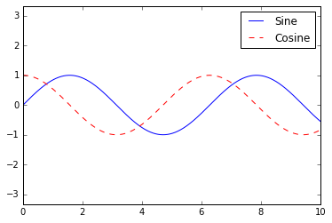
But there are many ways we might want to customize such a legend. For example, we can specify the location and turn off the frame (Figure 4-42):
In[4]:ax.legend(loc='upper left',frameon=False)fig
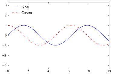
We can use the ncol command to specify the number of columns in the
legend (Figure 4-43):
In[5]:ax.legend(frameon=False,loc='lower center',ncol=2)fig
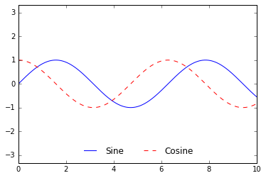
We can use a rounded box (fancybox) or add a shadow, change the
transparency (alpha value) of the frame, or change the padding around
the text (Figure 4-44):
In[6]:ax.legend(fancybox=True,framealpha=1,shadow=True,borderpad=1)fig
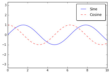
For more information on available legend options, see the plt.legend
docstring.
As we’ve already seen, the legend includes all labeled elements by default.
If this is not what is desired, we can fine-tune which elements and
labels appear in the legend by using the objects returned by plot
commands. The plt.plot() command is able to create multiple lines at
once, and returns a list of created line instances. Passing any of these
to plt.legend() will tell it which to identify, along with the labels
we’d like to specify (Figure 4-45):
In[7]:y=np.sin(x[:,np.newaxis]+np.pi*np.arange(0,2,0.5))lines=plt.plot(x,y)# lines is a list of plt.Line2D instancesplt.legend(lines[:2],['first','second']);

I generally find in practice that it is clearer to use the first method, applying labels to the plot elements you’d like to show on the legend (Figure 4-46):
In[8]:plt.plot(x,y[:,0],label='first')plt.plot(x,y[:,1],label='second')plt.plot(x,y[:,2:])plt.legend(framealpha=1,frameon=True);
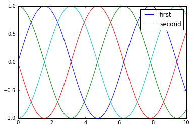
Notice that by default, the legend ignores all elements without a
label attribute set.
Sometimes the legend defaults are not sufficient for the given visualization. For example, perhaps you’re using the size of points to mark certain features of the data, and want to create a legend reflecting this. Here is an example where we’ll use the size of points to indicate populations of California cities. We’d like a legend that specifies the scale of the sizes of the points, and we’ll accomplish this by plotting some labeled data with no entries (Figure 4-47):
In[9]:importpandasaspdcities=pd.read_csv('data/california_cities.csv')# Extract the data we're interested inlat,lon=cities['latd'],cities['longd']population,area=cities['population_total'],cities['area_total_km2']# Scatter the points, using size and color but no labelplt.scatter(lon,lat,label=None,c=np.log10(population),cmap='viridis',s=area,linewidth=0,alpha=0.5)plt.axis(aspect='equal')plt.xlabel('longitude')plt.ylabel('latitude')plt.colorbar(label='log$_{10}$(population)')plt.clim(3,7)# Here we create a legend:# we'll plot empty lists with the desired size and labelforareain[100,300,500]:plt.scatter([],[],c='k',alpha=0.3,s=area,label=str(area)+' km$^2$')plt.legend(scatterpoints=1,frameon=False,labelspacing=1,title='City Area')plt.title('California Cities: Area and Population');
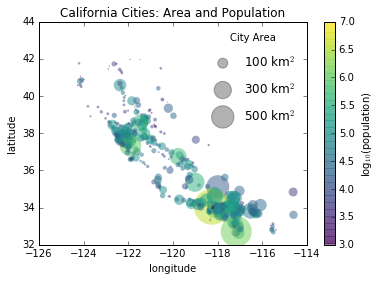
The legend will always reference some object that is on the plot, so if we’d like to display a particular shape we need to plot it. In this case, the objects we want (gray circles) are not on the plot, so we fake them by plotting empty lists. Notice too that the legend only lists plot elements that have a label specified.
By plotting empty lists, we create labeled plot objects that are picked up by the legend, and now our legend tells us some useful information. This strategy can be useful for creating more sophisticated visualizations.
Finally, note that for geographic data like this, it would be clearer if we could show state boundaries or other map-specific elements. For this, an excellent choice of tool is Matplotlib’s Basemap add-on toolkit, which we’ll explore in “Geographic Data with Basemap”.
Sometimes when designing a plot you’d like to add multiple legends to
the same axes. Unfortunately, Matplotlib does not make this easy: via
the standard legend interface, it is only possible to create a single
legend for the entire plot. If you try to create a second legend using
plt.legend() or ax.legend(), it will simply override the first one.
We can work around this by creating a new legend artist from scratch,
and then using the lower-level ax.add_artist() method to manually add
the second artist to the plot (Figure 4-48):
In[10]:fig,ax=plt.subplots()lines=[]styles=['-','--','-.',':']x=np.linspace(0,10,1000)foriinrange(4):lines+=ax.plot(x,np.sin(x-i*np.pi/2),styles[i],color='black')ax.axis('equal')# specify the lines and labels of the first legendax.legend(lines[:2],['line A','line B'],loc='upper right',frameon=False)# Create the second legend and add the artist manually.frommatplotlib.legendimportLegendleg=Legend(ax,lines[2:],['line C','line D'],loc='lower right',frameon=False)ax.add_artist(leg);
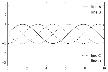
This is a peek into the low-level artist objects that compose any
Matplotlib plot. If you examine the source code of ax.legend() (recall
that you can do this within the IPython notebook using ax.legend??)
you’ll see that the function simply consists of some logic to create a
suitable Legend artist, which is then saved in the legend_ attribute
and added to the figure when the plot is drawn.
Plot legends identify discrete labels of discrete points. For continuous labels based on the color of points, lines, or regions, a labeled colorbar can be a great tool. In Matplotlib, a colorbar is a separate axes that can provide a key for the meaning of colors in a plot. Because the book is printed in black and white, this section has an accompanying online appendix where you can view the figures in full color (https://github.com/jakevdp/PythonDataScienceHandbook). We’ll start by setting up the notebook for plotting and importing the functions we will use:
In[1]:importmatplotlib.pyplotaspltplt.style.use('classic')
In[2]:%matplotlibinlineimportnumpyasnp
As we have seen several times throughout this section, the simplest
colorbar can be created with the plt.colorbar function (Figure 4-49):
In[3]:x=np.linspace(0,10,1000)I=np.sin(x)*np.cos(x[:,np.newaxis])plt.imshow(I)plt.colorbar();
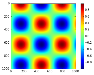
We’ll now discuss a few ideas for customizing these colorbars and using them effectively in various situations.
We can specify the colormap using the cmap argument to the plotting
function that is creating the visualization (Figure 4-50):
In[4]:plt.imshow(I,cmap='gray');
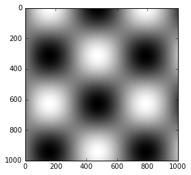
All the available colormaps are in the plt.cm namespace; using
IPython’s tab-completion feature will give you a full list of built-in
possibilities:
plt.cm.<TAB>
But being able to choose a colormap is just the first step: more important is how to decide among the possibilities! The choice turns out to be much more subtle than you might initially expect.
A full treatment of color choice within visualization is beyond the scope of this book, but for entertaining reading on this subject and others, see the article “Ten Simple Rules for Better Figures”. Matplotlib’s online documentation also has an interesting discussion of colormap choice.
Broadly, you should be aware of three different categories of colormaps:
These consist of one continuous sequence
of colors (e.g., binary or viridis).
These usually contain two distinct colors,
which show positive and negative deviations from a mean (e.g., RdBu or
PuOr).
These mix colors with no particular
sequence (e.g., rainbow or jet).
The jet colormap, which was the default in Matplotlib prior to version
2.0, is an example of a qualitative colormap. Its status as the default
was quite unfortunate, because qualitative maps are often a poor choice
for representing quantitative data. Among the problems is the fact that
qualitative maps usually do not display any uniform progression in
brightness as the scale increases.
We can see this by converting the jet colorbar into black and white (Figure 4-51):
In[5]:frommatplotlib.colorsimportLinearSegmentedColormapdefgrayscale_cmap(cmap):"""Return a grayscale version of the given colormap"""cmap=plt.cm.get_cmap(cmap)colors=cmap(np.arange(cmap.N))# convert RGBA to perceived grayscale luminance# cf. http://alienryderflex.com/hsp.htmlRGB_weight=[0.299,0.587,0.114]luminance=np.sqrt(np.dot(colors[:,:3]**2,RGB_weight))colors[:,:3]=luminance[:,np.newaxis]returnLinearSegmentedColormap.from_list(cmap.name+"_gray",colors,cmap.N)defview_colormap(cmap):"""Plot a colormap with its grayscale equivalent"""cmap=plt.cm.get_cmap(cmap)colors=cmap(np.arange(cmap.N))cmap=grayscale_cmap(cmap)grayscale=cmap(np.arange(cmap.N))fig,ax=plt.subplots(2,figsize=(6,2),subplot_kw=dict(xticks=[],yticks=[]))ax[0].imshow([colors],extent=[0,10,0,1])ax[1].imshow([grayscale],extent=[0,10,0,1])
In[6]:view_colormap('jet')

Notice the bright stripes in the grayscale image. Even in full color,
this uneven brightness means that the eye will be drawn to certain
portions of the color range, which will potentially emphasize
unimportant parts of the dataset. It’s better to use a colormap such as
viridis (the default as of Matplotlib 2.0), which is specifically
constructed to have an even brightness variation across the range. Thus,
it not only plays well with our color perception, but also will
translate well to grayscale printing (Figure 4-52):
In[7]:view_colormap('viridis')

If you favor rainbow schemes, another good option for continuous data is
the cubehelix colormap (Figure 4-53):
In[8]:view_colormap('cubehelix')

For other situations, such as showing positive and negative deviations
from some mean, dual-color colorbars such as RdBu (short for Red-Blue) can be
useful. However, as you can see in Figure 4-54, it’s important to note that the positive-negative information will be
lost upon translation to grayscale!
In[9]:view_colormap('RdBu')

We’ll see examples of using some of these color maps as we continue.
There are a large number of colormaps available in Matplotlib; to see a
list of them, you can use IPython to explore the plt.cm submodule. For
a more principled approach to colors in Python, you can refer to the
tools and documentation within the Seaborn library (see
“Visualization with Seaborn”).
Matplotlib allows for a large range of colorbar customization. The
colorbar itself is simply an instance of plt.Axes, so all of the axes
and tick formatting tricks we’ve learned are applicable. The colorbar
has some interesting flexibility; for example, we can narrow the color
limits and indicate the out-of-bounds values with a triangular arrow at
the top and bottom by setting the extend property. This might come in
handy, for example, if you’re displaying an image that is subject to noise (Figure 4-55):
In[10]:# make noise in 1% of the image pixelsspeckles=(np.random.random(I.shape)<0.01)I[speckles]=np.random.normal(0,3,np.count_nonzero(speckles))plt.figure(figsize=(10,3.5))plt.subplot(1,2,1)plt.imshow(I,cmap='RdBu')plt.colorbar()plt.subplot(1,2,2)plt.imshow(I,cmap='RdBu')plt.colorbar(extend='both')plt.clim(-1,1);
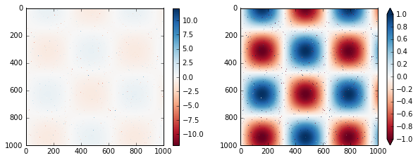
Notice that in the left panel, the default color limits respond to the noisy pixels, and the range of the noise completely washes out the pattern we are interested in. In the right panel, we manually set the color limits, and add extensions to indicate values that are above or below those limits. The result is a much more useful visualization of our data.
Colormaps are by default continuous, but sometimes you’d like to
represent discrete values. The easiest way to do this is to use the
plt.cm.get_cmap() function, and pass the name of a suitable colormap
along with the number of desired bins (Figure 4-56):
In[11]:plt.imshow(I,cmap=plt.cm.get_cmap('Blues',6))plt.colorbar()plt.clim(-1,1);
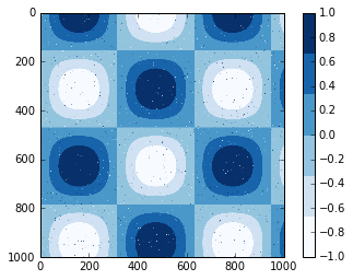
The discrete version of a colormap can be used just like any other colormap.
For an example of where this might be useful, let’s look at an interesting visualization of some handwritten digits data. This data is included in Scikit-Learn, and consists of nearly 2,000 8×8 thumbnails showing various handwritten digits.
For now, let’s start by downloading the digits data and visualizing
several of the example images with plt.imshow() (Figure 4-57):
In[12]:# load images of the digits 0 through 5 and visualize several of themfromsklearn.datasetsimportload_digitsdigits=load_digits(n_class=6)fig,ax=plt.subplots(8,8,figsize=(6,6))fori,axiinenumerate(ax.flat):axi.imshow(digits.images[i],cmap='binary')axi.set(xticks=[],yticks=[])
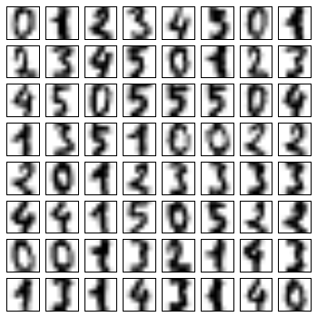
Because each digit is defined by the hue of its 64 pixels, we can consider each digit to be a point lying in 64-dimensional space: each dimension represents the brightness of one pixel. But visualizing relationships in such high-dimensional spaces can be extremely difficult. One way to approach this is to use a dimensionality reduction technique such as manifold learning to reduce the dimensionality of the data while maintaining the relationships of interest. Dimensionality reduction is an example of unsupervised machine learning, and we will discuss it in more detail in “What Is Machine Learning?”.
Deferring the discussion of these details, let’s take a look at a two-dimensional manifold learning projection of this digits data (see “In-Depth: Manifold Learning” for details):
In[13]:# project the digits into 2 dimensions using IsoMapfromsklearn.manifoldimportIsomapiso=Isomap(n_components=2)projection=iso.fit_transform(digits.data)
We’ll use our discrete colormap to view the results, setting the ticks
and clim to improve the aesthetics of the resulting colorbar (Figure 4-58):
In[14]:# plot the resultsplt.scatter(projection[:,0],projection[:,1],lw=0.1,c=digits.target,cmap=plt.cm.get_cmap('cubehelix',6))plt.colorbar(ticks=range(6),label='digit value')plt.clim(-0.5,5.5)
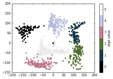
The projection also gives us some interesting insights on the relationships within the dataset: for example, the ranges of 5 and 3 nearly overlap in this projection, indicating that some handwritten fives and threes are difficult to distinguish, and therefore more likely to be confused by an automated classification algorithm. Other values, like 0 and 1, are more distantly separated, and therefore much less likely to be confused. This observation agrees with our intuition, because 5 and 3 look much more similar than do 0 and 1.
We’ll return to manifold learning and digit classification in Chapter 5.
Sometimes it is helpful to compare different views of data side by side. To this end, Matplotlib has the concept of subplots: groups of smaller axes that can exist together within a single figure. These subplots might be insets, grids of plots, or other more complicated layouts. In this section, we’ll explore four routines for creating subplots in Matplotlib. We’ll start by setting up the notebook for plotting and importing the functions we will use:
In[1]:%matplotlibinlineimportmatplotlib.pyplotaspltplt.style.use('seaborn-white')importnumpyasnp
The most basic method of creating an axes is to use the plt.axes
function. As we’ve seen previously, by default this creates a standard
axes object that fills the entire figure. plt.axes also takes an
optional argument that is a list of four numbers in the figure
coordinate system. These numbers represent
[bottom, left, width, height] in the figure coordinate system, which
ranges from 0 at the bottom left of the figure to 1 at the top right of
the figure.
For example, we might create an inset axes at the top-right corner of another axes by setting the x and y position to 0.65 (that is, starting at 65% of the width and 65% of the height of the figure) and the x and y extents to 0.2 (that is, the size of the axes is 20% of the width and 20% of the height of the figure). Figure 4-59 shows the result of this code:
In[2]:ax1=plt.axes()# standard axesax2=plt.axes([0.65,0.65,0.2,0.2])
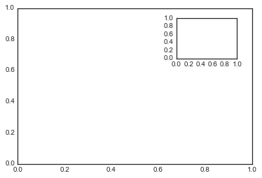
The equivalent of this command within the object-oriented interface is
fig.add_axes(). Let’s use this to create two vertically stacked axes (Figure 4-60):
In[3]:fig=plt.figure()ax1=fig.add_axes([0.1,0.5,0.8,0.4],xticklabels=[],ylim=(-1.2,1.2))ax2=fig.add_axes([0.1,0.1,0.8,0.4],ylim=(-1.2,1.2))x=np.linspace(0,10)ax1.plot(np.sin(x))ax2.plot(np.cos(x));
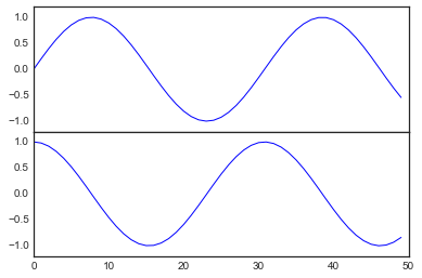
We now have two axes (the top with no tick labels) that are just touching: the bottom of the upper panel (at position 0.5) matches the top of the lower panel (at position 0.1 + 0.4).
Aligned columns or rows of subplots are a common enough need that
Matplotlib has several convenience routines that make them easy to
create. The lowest level of these is plt.subplot(), which creates a
single subplot within a grid. As you can see, this command takes three
integer arguments—the number of rows, the number of columns, and the
index of the plot to be created in this scheme, which runs from the
upper left to the bottom right (Figure 4-61):
In[4]:foriinrange(1,7):plt.subplot(2,3,i)plt.text(0.5,0.5,str((2,3,i)),fontsize=18,ha='center')
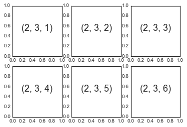
The command plt.subplots_adjust can be used to adjust the spacing between these plots. The following code (the result of which is shown in Figure 4-62) uses the equivalent object-oriented
command, fig.add_subplot():
In[5]:fig=plt.figure()fig.subplots_adjust(hspace=0.4,wspace=0.4)foriinrange(1,7):ax=fig.add_subplot(2,3,i)ax.text(0.5,0.5,str((2,3,i)),fontsize=18,ha='center')
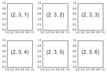
We’ve used the hspace and wspace arguments of plt.subplots_adjust,
which specify the spacing along the height and width of the figure, in
units of the subplot size (in this case, the space is 40% of the subplot
width and height).
The approach just described can become quite tedious when you’re creating a large grid of
subplots, especially if you’d like to hide the x- and y-axis labels
on the inner plots. For this purpose, plt.subplots() is the easier tool
to use (note the s at the end of subplots). Rather than creating a
single subplot, this function creates a full grid of subplots in a
single line, returning them in a NumPy array. The arguments are the
number of rows and number of columns, along with optional keywords
sharex and sharey, which allow you to specify the relationships
between different axes.
Here we’ll create a 2×3 grid of subplots, where all axes in the same row share their y-axis scale, and all axes in the same column share their x-axis scale (Figure 4-63):
In[6]:fig,ax=plt.subplots(2,3,sharex='col',sharey='row')

Note that by specifying sharex and sharey, we’ve automatically
removed inner labels on the grid to make the plot cleaner. The resulting
grid of axes instances is returned within a NumPy array, allowing for
convenient specification of the desired axes using standard array
indexing notation (Figure 4-64):
In[7]:# axes are in a two-dimensional array, indexed by [row, col]foriinrange(2):forjinrange(3):ax[i,j].text(0.5,0.5,str((i,j)),fontsize=18,ha='center')fig
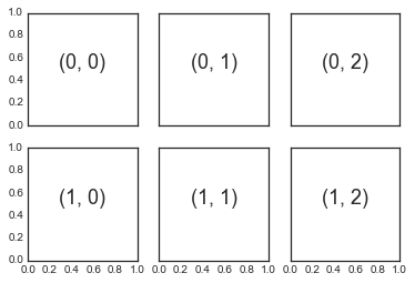
In comparison to plt.subplot(), plt.subplots() is more consistent
with Python’s conventional 0-based indexing.
To go beyond a regular grid to subplots that span multiple rows and
columns, plt.GridSpec() is the best tool. The plt.GridSpec() object
does not create a plot by itself; it is simply a convenient interface
that is recognized by the plt.subplot() command. For example, a
gridspec for a grid of two rows and three columns with some specified width
and height space looks like this:
In[8]:grid=plt.GridSpec(2,3,wspace=0.4,hspace=0.3)
From this we can specify subplot locations and extents using the familiar Python slicing syntax (Figure 4-65):
In[9]:plt.subplot(grid[0,0])plt.subplot(grid[0,1:])plt.subplot(grid[1,:2])plt.subplot(grid[1,2]);
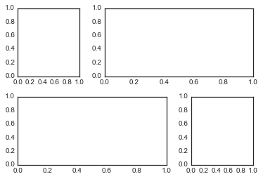
This type of flexible grid alignment has a wide range of uses. I most often use it when creating multi-axes histogram plots like the one shown here (Figure 4-66):
In[10]:# Create some normally distributed datamean=[0,0]cov=[[1,1],[1,2]]x,y=np.random.multivariate_normal(mean,cov,3000).T# Set up the axes with gridspecfig=plt.figure(figsize=(6,6))grid=plt.GridSpec(4,4,hspace=0.2,wspace=0.2)main_ax=fig.add_subplot(grid[:-1,1:])y_hist=fig.add_subplot(grid[:-1,0],xticklabels=[],sharey=main_ax)x_hist=fig.add_subplot(grid[-1,1:],yticklabels=[],sharex=main_ax)# scatter points on the main axesmain_ax.plot(x,y,'ok',markersize=3,alpha=0.2)# histogram on the attached axesx_hist.hist(x,40,histtype='stepfilled',orientation='vertical',color='gray')x_hist.invert_yaxis()y_hist.hist(y,40,histtype='stepfilled',orientation='horizontal',color='gray')y_hist.invert_xaxis()
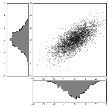
This type of distribution plotted alongside its margins is common enough that it has its own plotting API in the Seaborn package; see “Visualization with Seaborn” for more details.
Creating a good visualization involves guiding the reader so that the figure tells a story. In some cases, this story can be told in an entirely visual manner, without the need for added text, but in others, small textual cues and labels are necessary. Perhaps the most basic types of annotations you will use are axes labels and titles, but the options go beyond this. Let’s take a look at some data and how we might visualize and annotate it to help convey interesting information. We’ll start by setting up the notebook for plotting and importing the functions we will use:
In[1]:%matplotlibinlineimportmatplotlib.pyplotaspltimportmatplotlibasmplplt.style.use('seaborn-whitegrid')importnumpyasnpimportpandasaspd
Let’s return to some data we worked with earlier in “Example: Birthrate Data”, where we generated a plot of average births over the course of the calendar year; as already mentioned, this data can be downloaded at https://raw.githubusercontent.com/jakevdp/data-CDCbirths/master/births.csv.
We’ll start with the same cleaning procedure we used there, and plot the results (Figure 4-67):
In[2]:births=pd.read_csv('births.csv')quartiles=np.percentile(births['births'],[25,50,75])mu,sig=quartiles[1],0.74*(quartiles[2]-quartiles[0])births=births.query('(births > @mu - 5 * @sig) & (births < @mu + 5 * @sig)')births['day']=births['day'].astype(int)births.index=pd.to_datetime(10000*births.year+100*births.month+births.day,format='%Y%m%d')births_by_date=births.pivot_table('births',[births.index.month,births.index.day])births_by_date.index=[pd.datetime(2012,month,day)for(month,day)inbirths_by_date.index]
In[3]:fig,ax=plt.subplots(figsize=(12,4))births_by_date.plot(ax=ax);
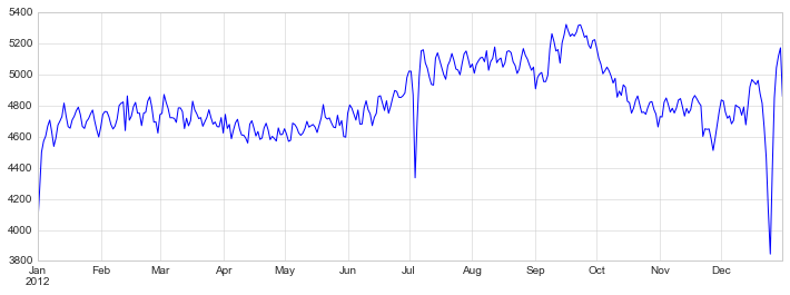
When we’re communicating data like this, it is often useful to annotate
certain features of the plot to draw the reader’s attention. This can be
done manually with the plt.text/ax.text command, which will place
text at a particular x/y value (Figure 4-68):
In[4]:fig,ax=plt.subplots(figsize=(12,4))births_by_date.plot(ax=ax)# Add labels to the plotstyle=dict(size=10,color='gray')ax.text('2012-1-1',3950,"New Year's Day",**style)ax.text('2012-7-4',4250,"Independence Day",ha='center',**style)ax.text('2012-9-4',4850,"Labor Day",ha='center',**style)ax.text('2012-10-31',4600,"Halloween",ha='right',**style)ax.text('2012-11-25',4450,"Thanksgiving",ha='center',**style)ax.text('2012-12-25',3850,"Christmas ",ha='right',**style)# Label the axesax.set(title='USA births by day of year (1969-1988)',ylabel='average daily births')# Format the x axis with centered month labelsax.xaxis.set_major_locator(mpl.dates.MonthLocator())ax.xaxis.set_minor_locator(mpl.dates.MonthLocator(bymonthday=15))ax.xaxis.set_major_formatter(plt.NullFormatter())ax.xaxis.set_minor_formatter(mpl.dates.DateFormatter('%h'));
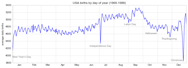
The ax.text method takes an x position, a y position, a string, and
then optional keywords specifying the color, size, style, alignment, and
other properties of the text. Here we used ha='right' and
ha='center', where ha is short for horizonal alignment. See the
docstring of plt.text() and of mpl.text.Text() for more information
on available options.
In the previous example, we anchored our text annotations to data locations. Sometimes it’s preferable to anchor the text to a position on the axes or figure, independent of the data. In Matplotlib, we do this by modifying the transform.
Any graphics display framework needs some scheme for translating between
coordinate systems. For example, a data point at
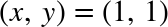 needs to somehow be represented at a
certain location on the figure, which in turn needs to be represented in
pixels on the screen. Mathematically, such coordinate transformations are relatively straightforward, and Matplotlib has a well-developed set of
tools that it uses internally to perform them (the tools can be explored in the
needs to somehow be represented at a
certain location on the figure, which in turn needs to be represented in
pixels on the screen. Mathematically, such coordinate transformations are relatively straightforward, and Matplotlib has a well-developed set of
tools that it uses internally to perform them (the tools can be explored in the matplotlib.transforms submodule).
The average user rarely needs to worry about the details of these transforms, but it is helpful knowledge to have when considering the placement of text on a figure. There are three predefined transforms that can be useful in this situation:
ax.transDataTransform associated with data coordinates
ax.transAxesTransform associated with the axes (in units of axes dimensions)
fig.transFigureTransform associated with the figure (in units of figure dimensions)
Here let’s look at an example of drawing text at various locations using these transforms (Figure 4-69):
In[5]:fig,ax=plt.subplots(facecolor='lightgray')ax.axis([0,10,0,10])# transform=ax.transData is the default, but we'll specify it anywayax.text(1,5,". Data: (1, 5)",transform=ax.transData)ax.text(0.5,0.1,". Axes: (0.5, 0.1)",transform=ax.transAxes)ax.text(0.2,0.2,". Figure: (0.2, 0.2)",transform=fig.transFigure);
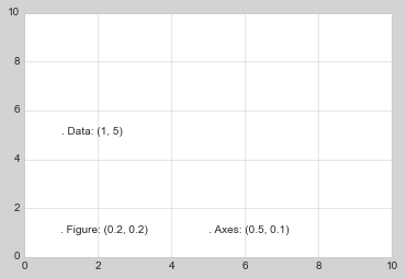
Note that by default, the text is aligned above and to the left of the specified coordinates; here the “.” at the beginning of each string will approximately mark the given coordinate location.
The transData coordinates give the usual data coordinates associated
with the x- and y-axis labels. The transAxes coordinates give the
location from the bottom-left corner of the axes (here the white box)
as a fraction of the axes size. The transFigure coordinates are
similar, but specify the position from the bottom left of the figure
(here the gray box) as a fraction of the figure size.
Notice now that if we change the axes limits, it is only the transData
coordinates that will be affected, while the others remain stationary (Figure 4-70):
In[6]:ax.set_xlim(0,2)ax.set_ylim(-6,6)fig
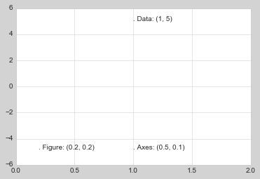
You can see this behavior more clearly by changing the axes limits
interactively; if you are executing this code in a notebook, you can
make that happen by changing %matplotlib inline to
%matplotlib notebook and using each plot’s menu to interact with the
plot.
Along with tick marks and text, another useful annotation mark is the simple arrow.
Drawing arrows in Matplotlib is often much harder than you might hope.
While there is a plt.arrow() function available, I wouldn’t suggest using
it; the arrows it creates are SVG objects that will be subject to the
varying aspect ratio of your plots, and the result is rarely what the
user intended. Instead, I’d suggest using the plt.annotate() function.
This function creates some text and an arrow, and the arrows can be very
flexibly specified.
Here we’ll use annotate with several of its options (Figure 4-71):
In[7]:%matplotlibinlinefig,ax=plt.subplots()x=np.linspace(0,20,1000)ax.plot(x,np.cos(x))ax.axis('equal')ax.annotate('local maximum',xy=(6.28,1),xytext=(10,4),arrowprops=dict(facecolor='black',shrink=0.05))ax.annotate('local minimum',xy=(5*np.pi,-1),xytext=(2,-6),arrowprops=dict(arrowstyle="->",connectionstyle="angle3,angleA=0,angleB=-90"));
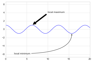
The arrow style is controlled through the arrowprops dictionary, which
has numerous options available. These options are fairly well documented
in Matplotlib’s online documentation, so rather than repeating them here
I’ll quickly show some of the possibilities.
Let’s demonstrate several of the possible options using the birthrate
plot from before (Figure 4-72):
In[8]:fig,ax=plt.subplots(figsize=(12,4))births_by_date.plot(ax=ax)# Add labels to the plotax.annotate("New Year's Day",xy=('2012-1-1',4100),xycoords='data',xytext=(50,-30),textcoords='offset points',arrowprops=dict(arrowstyle="->",connectionstyle="arc3,rad=-0.2"))ax.annotate("Independence Day",xy=('2012-7-4',4250),xycoords='data',bbox=dict(boxstyle="round",fc="none",ec="gray"),xytext=(10,-40),textcoords='offset points',ha='center',arrowprops=dict(arrowstyle="->"))ax.annotate('Labor Day',xy=('2012-9-4',4850),xycoords='data',ha='center',xytext=(0,-20),textcoords='offset points')ax.annotate('',xy=('2012-9-1',4850),xytext=('2012-9-7',4850),xycoords='data',textcoords='data',arrowprops={'arrowstyle':'|-|,widthA=0.2,widthB=0.2',})ax.annotate('Halloween',xy=('2012-10-31',4600),xycoords='data',xytext=(-80,-40),textcoords='offset points',arrowprops=dict(arrowstyle="fancy",fc="0.6",ec="none",connectionstyle="angle3,angleA=0,angleB=-90"))ax.annotate('Thanksgiving',xy=('2012-11-25',4500),xycoords='data',xytext=(-120,-60),textcoords='offset points',bbox=dict(boxstyle="round4,pad=.5",fc="0.9"),arrowprops=dict(arrowstyle="->",connectionstyle="angle,angleA=0,angleB=80,rad=20"))ax.annotate('Christmas',xy=('2012-12-25',3850),xycoords='data',xytext=(-30,0),textcoords='offset points',size=13,ha='right',va="center",bbox=dict(boxstyle="round",alpha=0.1),arrowprops=dict(arrowstyle="wedge,tail_width=0.5",alpha=0.1));# Label the axesax.set(title='USA births by day of year (1969-1988)',ylabel='average daily births')# Format the x axis with centered month labelsax.xaxis.set_major_locator(mpl.dates.MonthLocator())ax.xaxis.set_minor_locator(mpl.dates.MonthLocator(bymonthday=15))ax.xaxis.set_major_formatter(plt.NullFormatter())ax.xaxis.set_minor_formatter(mpl.dates.DateFormatter('%h'));ax.set_ylim(3600,5400);
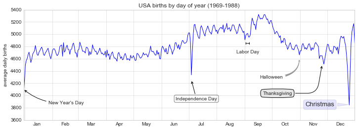
You’ll notice that the specifications of the arrows and text boxes are very detailed: this gives you the power to create nearly any arrow style you wish. Unfortunately, it also means that these sorts of features often must be manually tweaked, a process that can be very time-consuming when one is producing publication-quality graphics! Finally, I’ll note that the preceding mix of styles is by no means best practice for presenting data, but rather included as a demonstration of some of the available options.
More discussion and examples of available arrow and annotation styles can be found in the Matplotlib gallery, in particular http://matplotlib.org/examples/pylab_examples/annotation_demo2.html.
Matplotlib’s default tick locators and formatters are designed to be generally sufficient in many common situations, but are in no way optimal for every plot. This section will give several examples of adjusting the tick locations and formatting for the particular plot type you’re interested in.
Before we go into examples, it will be best for us to understand further
the object hierarchy of Matplotlib plots. Matplotlib aims to have a
Python object representing everything that appears on the plot: for
example, recall that the figure is the bounding box within which plot
elements appear. Each Matplotlib object can also act as a container of
sub-objects; for example, each figure can contain one or more axes
objects, each of which in turn contain other objects representing plot
contents.
The tick marks are no exception. Each axes has attributes xaxis and
yaxis, which in turn have attributes that contain all the properties
of the lines, ticks, and labels that make up the axes.
Within each axis, there is the concept of a major tick mark and a minor tick mark. As the names would imply, major ticks are usually bigger or more pronounced, while minor ticks are usually smaller. By default, Matplotlib rarely makes use of minor ticks, but one place you can see them is within logarithmic plots (Figure 4-73):
In[1]:%matplotlibinlineimportmatplotlib.pyplotaspltplt.style.use('seaborn-whitegrid')importnumpyasnp
In[2]:ax=plt.axes(xscale='log',yscale='log')
We see here that each major tick shows a large tick mark and a label, while each minor tick shows a smaller tick mark with no label.
We can customize these tick properties—that is, locations and labels—by
setting the formatter and locator objects of each axis. Let’s
examine these for the x axis of the plot just shown:
In[3]:(ax.xaxis.get_major_locator())(ax.xaxis.get_minor_locator())
<matplotlib.ticker.LogLocator object at 0x107530cc0> <matplotlib.ticker.LogLocator object at 0x107530198>
In[4]:(ax.xaxis.get_major_formatter())(ax.xaxis.get_minor_formatter())
<matplotlib.ticker.LogFormatterMathtext object at 0x107512780> <matplotlib.ticker.NullFormatter object at 0x10752dc18>
We see that both major and minor tick labels have their locations
specified by a LogLocator (which makes sense for a logarithmic plot).
Minor ticks, though, have their labels formatted by a NullFormatter;
this says that no labels will be shown.
We’ll now show a few examples of setting these locators and formatters for various plots.
Perhaps the most common tick/label formatting operation is the act of
hiding ticks or labels. We can do this using plt.NullLocator() and
plt.NullFormatter(), as shown here (Figure 4-74):
In[5]:ax=plt.axes()ax.plot(np.random.rand(50))ax.yaxis.set_major_locator(plt.NullLocator())ax.xaxis.set_major_formatter(plt.NullFormatter())
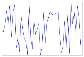
Notice that we’ve removed the labels (but kept the ticks/gridlines) from the x axis, and removed the ticks (and thus the labels as well) from the y axis. Having no ticks at all can be useful in many situations—for example, when you want to show a grid of images. For instance, consider Figure 4-75, which includes images of different faces, an example often used in supervised machine learning problems (for more information, see “In-Depth: Support Vector Machines”):
In[6]:fig,ax=plt.subplots(5,5,figsize=(5,5))fig.subplots_adjust(hspace=0,wspace=0)# Get some face data from scikit-learnfromsklearn.datasetsimportfetch_olivetti_facesfaces=fetch_olivetti_faces().imagesforiinrange(5):forjinrange(5):ax[i,j].xaxis.set_major_locator(plt.NullLocator())ax[i,j].yaxis.set_major_locator(plt.NullLocator())ax[i,j].imshow(faces[10*i+j],cmap="bone")
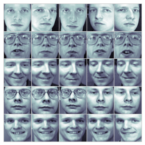
Notice that each image has its own axes, and we’ve set the locators to null because the tick values (pixel number in this case) do not convey relevant information for this particular visualization.
One common problem with the default settings is that smaller subplots can end up with crowded labels. We can see this in the plot grid shown in Figure 4-76:
In[7]:fig,ax=plt.subplots(4,4,sharex=True,sharey=True)

Particularly for the x ticks, the numbers nearly overlap, making them
quite difficult to decipher. We can fix this with the
plt.MaxNLocator(), which allows us to specify the maximum number of
ticks that will be displayed. Given this maximum number, Matplotlib
will use internal logic to choose the particular tick locations (Figure 4-77):
In[8]:# For every axis, set the x and y major locatorforaxiinax.flat:axi.xaxis.set_major_locator(plt.MaxNLocator(3))axi.yaxis.set_major_locator(plt.MaxNLocator(3))fig
This makes things much cleaner. If you want even more control over the
locations of regularly spaced ticks, you might also use
plt.MultipleLocator, which we’ll discuss in the following section.
Matplotlib’s default tick formatting can leave a lot to be desired; it works well as a broad default, but sometimes you’d like to do something more. Consider the plot shown in Figure 4-78, a sine and a cosine:
In[9]:# Plot a sine and cosine curvefig,ax=plt.subplots()x=np.linspace(0,3*np.pi,1000)ax.plot(x,np.sin(x),lw=3,label='Sine')ax.plot(x,np.cos(x),lw=3,label='Cosine')# Set up grid, legend, and limitsax.grid(True)ax.legend(frameon=False)ax.axis('equal')ax.set_xlim(0,3*np.pi);
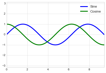
There are a couple changes we might like to make. First, it’s more
natural for this data to space the ticks and grid lines in multiples of
 . We can do this by setting a
 MultipleLocator, which
locates ticks at a multiple of the number you provide. For good measure,
we’ll add both major and minor ticks in multiples of
 (Figure 4-79):
In[10]:ax.xaxis.set_major_locator(plt.MultipleLocator(np.pi/2))ax.xaxis.set_minor_locator(plt.MultipleLocator(np.pi/4))fig
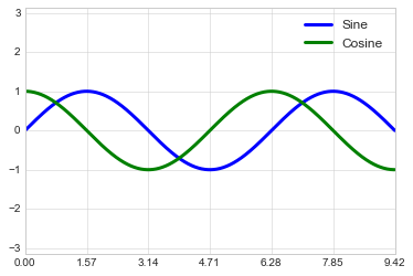
But now these tick labels look a little bit silly: we can see that they
are multiples of  , but the decimal representation does
not immediately convey this. To fix this, we can change the tick
formatter. There’s no built-in formatter for what we want to do, so
we’ll instead use
, but the decimal representation does
not immediately convey this. To fix this, we can change the tick
formatter. There’s no built-in formatter for what we want to do, so
we’ll instead use plt.FuncFormatter, which accepts a user-defined
function giving fine-grained control over the tick outputs (Figure 4-80):
In[11]:defformat_func(value,tick_number):# find number of multiples of pi/2N=int(np.round(2*value/np.pi))ifN==0:return"0"elifN==1:returnr"$\pi/2$"elifN==2:returnr"$\pi$"elifN%2>0:returnr"${0}\pi/2$".format(N)else:returnr"${0}\pi$".format(N//2)ax.xaxis.set_major_formatter(plt.FuncFormatter(format_func))fig
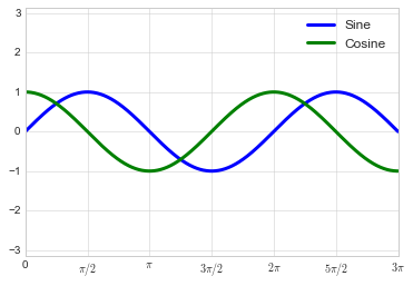
This is much better! Notice that we’ve made use of Matplotlib’s
LaTeX support, specified by enclosing the string within dollar signs.
This is very convenient for display of mathematical symbols and
formulae; in this case, "$\pi$" is rendered as the Greek character
 .
.
The plt.FuncFormatter() offers extremely fine-grained control over the
appearance of your plot ticks, and comes in very handy when you’re preparing
plots for presentation or publication.
We’ve mentioned a couple of the available formatters and locators. We’ll
conclude this section by briefly listing all the built-in locator and formatter
options. For more information on any of these, refer to the docstrings
or to the Matplotlib online documentation. Each of the following is
available in the plt namespace:
| Locator class | Description |
|---|---|
|
No ticks |
|
Tick locations are fixed |
|
Locator for index plots (e.g., where |
|
Evenly spaced ticks from |
|
Logarithmically ticks from |
|
Ticks and range are a multiple of base |
|
Finds up to a max number of ticks at nice locations |
|
(Default) |
|
Locator for minor ticks |
| Formatter class | Description |
|---|---|
|
No labels on the ticks |
|
Set the strings from a list of labels |
|
Set the strings manually for the labels |
|
User-defined function sets the labels |
|
Use a format string for each value |
|
(Default) Formatter for scalar values |
|
Default formatter for log axes |
We’ll see additional examples of these throughout the remainder of the book.
Matplotlib’s default plot settings are often the subject of complaint among its users. While much is slated to change in the 2.0 Matplotlib release, the ability to customize default settings helps bring the package in line with your own aesthetic preferences.
Here we’ll walk through some of Matplotlib’s runtime configuration (rc)
options, and take a look at the newer stylesheets feature, which
contains some nice sets of default configurations.
Throughout this chapter, we’ve seen how it is possible to tweak individual plot settings to end up with something that looks a little bit nicer than the default. It’s possible to do these customizations for each individual plot. For example, here is a fairly drab default histogram (Figure 4-81):
In[1]:importmatplotlib.pyplotaspltplt.style.use('classic')importnumpyasnp%matplotlibinline
In[2]:x=np.random.randn(1000)plt.hist(x);
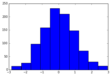
We can adjust this by hand to make it a much more visually pleasing plot, shown in Figure 4-82:
In[3]:# use a gray backgroundax=plt.axes(axisbg='#E6E6E6')ax.set_axisbelow(True)# draw solid white grid linesplt.grid(color='w',linestyle='solid')# hide axis spinesforspineinax.spines.values():spine.set_visible(False)# hide top and right ticksax.xaxis.tick_bottom()ax.yaxis.tick_left()# lighten ticks and labelsax.tick_params(colors='gray',direction='out')fortickinax.get_xticklabels():tick.set_color('gray')fortickinax.get_yticklabels():tick.set_color('gray')# control face and edge color of histogramax.hist(x,edgecolor='#E6E6E6',color='#EE6666');

This looks better, and you may recognize the look as inspired by the
look of the R language’s ggplot visualization package. But this took a
whole lot of effort! We definitely do not want to have to do all that
tweaking each time we create a plot. Fortunately, there is a way to
adjust these defaults once in a way that will work for all plots.
Each time Matplotlib loads, it defines a runtime configuration (rc) containing the default styles for every plot element you create.
You can adjust this configuration at any time using the plt.rc
convenience routine. Let’s see what it looks like to modify the rc
parameters so that our default plot will look similar to what we did
before.
We’ll start by saving a copy of the current rcParams dictionary, so we
can easily reset these changes in the current session:
In[4]:IPython_default=plt.rcParams.copy()
Now we can use the plt.rc function to change some of these settings:
In[5]:frommatplotlibimportcyclercolors=cycler('color',['#EE6666','#3388BB','#9988DD','#EECC55','#88BB44','#FFBBBB'])plt.rc('axes',facecolor='#E6E6E6',edgecolor='none',axisbelow=True,grid=True,prop_cycle=colors)plt.rc('grid',color='w',linestyle='solid')plt.rc('xtick',direction='out',color='gray')plt.rc('ytick',direction='out',color='gray')plt.rc('patch',edgecolor='#E6E6E6')plt.rc('lines',linewidth=2)
With these settings defined, we can now create a plot and see our settings in action (Figure 4-83):
In[6]:plt.hist(x);
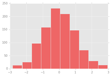
Let’s see what simple line plots look like with these rc parameters (Figure 4-84):
In[7]:foriinrange(4):plt.plot(np.random.rand(10))
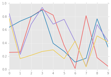
I find this much more aesthetically pleasing than the default styling.
If you disagree with my aesthetic sense, the good news is that you can
adjust the rc parameters to suit your own tastes! These settings can be
saved in a .matplotlibrc file, which you can read about in the
Matplotlib documentation.
That said, I prefer to customize Matplotlib using its
stylesheets instead.
The version 1.4 release of Matplotlib in August 2014 added a very
convenient style module, which includes a number of new default
stylesheets, as well as the ability to create and package your own
styles. These stylesheets are formatted similarly to the .matplotlibrc
files mentioned earlier, but must be named with a .mplstyle extension.
Even if you don’t create your own style, the stylesheets included by
default are extremely useful. The available styles are listed in
plt.style.available—here I’ll list only the first five for brevity:
In[8]:plt.style.available[:5]
Out[8]: ['fivethirtyeight',
'seaborn-pastel',
'seaborn-whitegrid',
'ggplot',
'grayscale']
The basic way to switch to a stylesheet is to call:
plt.style.use('stylename')
But keep in mind that this will change the style for the rest of the session! Alternatively, you can use the style context manager, which sets a style temporarily:
withplt.style.context('stylename'):make_a_plot()
Let’s create a function that will make two basic types of plot:
In[9]:defhist_and_lines():np.random.seed(0)fig,ax=plt.subplots(1,2,figsize=(11,4))ax[0].hist(np.random.randn(1000))foriinrange(3):ax[1].plot(np.random.rand(10))ax[1].legend(['a','b','c'],loc='lower left')
We’ll use this to explore how these plots look using the various built-in styles.
The default style is what we’ve been seeing so far throughout the book; we’ll start with that. First, let’s reset our runtime configuration to the notebook default:
In[10]:# reset rcParamsplt.rcParams.update(IPython_default);
Now let’s see how it looks (Figure 4-85):
In[11]:hist_and_lines()
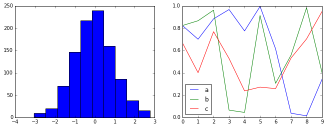
The FiveThirtyEight style mimics the graphics found on the popular FiveThirtyEight website. As you can see in Figure 4-86, it is typified by bold colors, thick lines, and transparent axes.
In[12]:withplt.style.context('fivethirtyeight'):hist_and_lines()
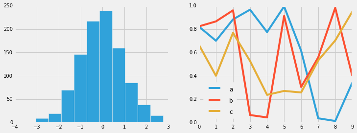
The ggplot package in the R language is a very popular visualization
tool. Matplotlib’s ggplot style mimics the default styles from that
package (Figure 4-87):
In[13]:withplt.style.context('ggplot'):hist_and_lines()
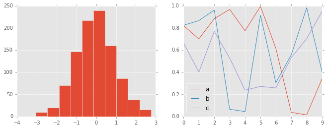
There is a very nice short online book called
Probabilistic
Programming and Bayesian Methods for Hackers; it features figures
created with Matplotlib, and uses a nice set of rc parameters to create
a consistent and visually appealing style throughout the book. This
style is reproduced in the bmh stylesheet (Figure 4-88):
In[14]:withplt.style.context('bmh'):hist_and_lines()
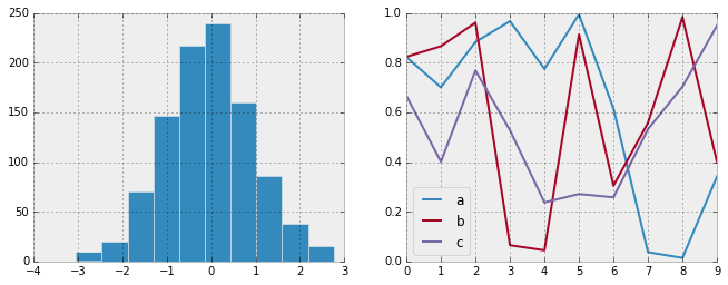
For figures used within presentations, it is often useful to have a dark
rather than light background. The dark_background style provides
this (Figure 4-89):
In[15]:withplt.style.context('dark_background'):hist_and_lines()
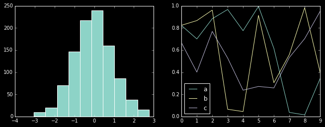
Sometimes you might find yourself preparing figures for a print
publication that does not accept color figures. For this, the
grayscale style, shown in Figure 4-90, can be very useful:
In[16]:withplt.style.context('grayscale'):hist_and_lines()
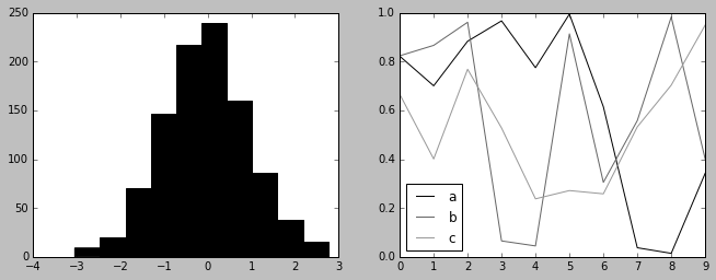
Matplotlib also has stylesheets inspired by the Seaborn library (discussed more fully in “Visualization with Seaborn”). As we will see, these styles are loaded automatically when Seaborn is imported into a notebook. I’ve found these settings to be very nice, and tend to use them as defaults in my own data exploration (see Figure 4-91):
In[17]:importseabornhist_and_lines()
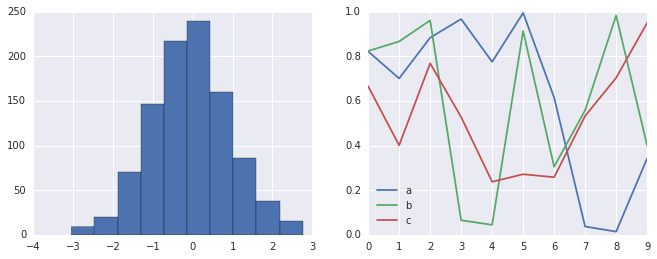
With all of these built-in options for various plot styles, Matplotlib becomes much more useful for both interactive visualization and creation of figures for publication. Throughout this book, I will generally use one or more of these style conventions when creating plots.
Matplotlib was initially designed with only two-dimensional plotting in
mind. Around the time of the 1.0 release, some three-dimensional plotting utilities
were built on top of Matplotlib’s two-dimensional display, and the result is a
convenient (if somewhat limited) set of tools for three-dimensional data
visualization. We enable three-dimensional plots by importing the mplot3d toolkit,
included with the main Matplotlib installation (Figure 4-92):
In[1]:frommpl_toolkitsimportmplot3d
Once this submodule is imported, we can create a three-dimensional axes by passing the keyword projection='3d' to any of the normal axes
creation routines:
In[2]:%matplotlibinlineimportnumpyasnpimportmatplotlib.pyplotasplt
In[3]:fig=plt.figure()ax=plt.axes(projection='3d')
With this 3D axes enabled, we can now plot a variety of
three-dimensional plot types. Three-dimensional plotting is one of the
functionalities that benefits immensely from viewing figures
interactively rather than statically in the notebook; recall that to use
interactive figures, you can use %matplotlib notebook rather than
%matplotlib inline when running this code.
The most basic three-dimensional plot is a line or scatter plot created
from sets of (x, y, z) triples. In analogy with the more common
two-dimensional plots discussed earlier, we can create these using the
ax.plot3D and ax.scatter3D functions. The call signature for these
is nearly identical to that of their two-dimensional counterparts, so
you can refer to “Simple Line Plots”
and “Simple Scatter Plots” for more
information on controlling the output. Here we’ll plot a trigonometric
spiral, along with some points drawn randomly near the line (Figure 4-93):
In[4]:ax=plt.axes(projection='3d')# Data for a three-dimensional linezline=np.linspace(0,15,1000)xline=np.sin(zline)yline=np.cos(zline)ax.plot3D(xline,yline,zline,'gray')# Data for three-dimensional scattered pointszdata=15*np.random.random(100)xdata=np.sin(zdata)+0.1*np.random.randn(100)ydata=np.cos(zdata)+0.1*np.random.randn(100)ax.scatter3D(xdata,ydata,zdata,c=zdata,cmap='Greens');
Notice that by default, the scatter points have their transparency adjusted to give a sense of depth on the page. While the three-dimensional effect is sometimes difficult to see within a static image, an interactive view can lead to some nice intuition about the layout of the points.
Analogous to the contour plots we explored in
“Density and Contour Plots”,
mplot3d contains tools to create three-dimensional relief plots using
the same inputs. Like two-dimensional ax.contour plots, ax.contour3D
requires all the input data to be in the form of two-dimensional regular
grids, with the Z data evaluated at each point. Here we’ll show a three-dimensional
contour diagram of a three-dimensional sinusoidal function (Figure 4-94):
In[5]:deff(x,y):returnnp.sin(np.sqrt(x**2+y**2))x=np.linspace(-6,6,30)y=np.linspace(-6,6,30)X,Y=np.meshgrid(x,y)Z=f(X,Y)
In[6]:fig=plt.figure()ax=plt.axes(projection='3d')ax.contour3D(X,Y,Z,50,cmap='binary')ax.set_xlabel('x')ax.set_ylabel('y')ax.set_zlabel('z');
Sometimes the default viewing angle is not optimal, in which case we can
use the view_init method to set the elevation and azimuthal angles.
In this example (the result of which is shown in Figure 4-95), we’ll use an elevation of 60 degrees (that is, 60 degrees above the
x-y plane) and an azimuth of 35 degrees (that is, rotated 35 degrees
counter-clockwise about the z-axis):
In[7]:ax.view_init(60,35)fig
Again, note that we can accomplish this type of rotation interactively by clicking and dragging when using one of Matplotlib’s interactive backends.
Two other types of three-dimensional plots that work on gridded data are wireframes and surface plots. These take a grid of values and project it onto the specified three-dimensional surface, and can make the resulting three-dimensional forms quite easy to visualize. Here’s an example using a wireframe (Figure 4-96):
In[8]:fig=plt.figure()ax=plt.axes(projection='3d')ax.plot_wireframe(X,Y,Z,color='black')ax.set_title('wireframe');
A surface plot is like a wireframe plot, but each face of the wireframe is a filled polygon. Adding a colormap to the filled polygons can aid perception of the topology of the surface being visualized (Figure 4-97):
In[9]:ax=plt.axes(projection='3d')ax.plot_surface(X,Y,Z,rstride=1,cstride=1,cmap='viridis',edgecolor='none')ax.set_title('surface');
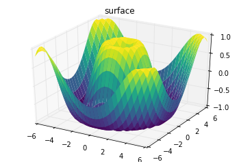
Note that though the grid of values for a surface plot needs to be
two-dimensional, it need not be rectilinear. Here is an example of
creating a partial polar grid, which when used with the surface3D plot
can give us a slice into the function we’re visualizing (Figure 4-98):
In[10]:r=np.linspace(0,6,20)theta=np.linspace(-0.9*np.pi,0.8*np.pi,40)r,theta=np.meshgrid(r,theta)X=r*np.sin(theta)Y=r*np.cos(theta)Z=f(X,Y)ax=plt.axes(projection='3d')ax.plot_surface(X,Y,Z,rstride=1,cstride=1,cmap='viridis',edgecolor='none');
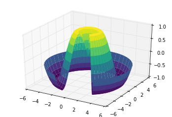
For some applications, the evenly sampled grids required by the preceding routines are overly restrictive and inconvenient. In these situations, the triangulation-based plots can be very useful. What if rather than an even draw from a Cartesian or a polar grid, we instead have a set of random draws?
In[11]:theta=2*np.pi*np.random.random(1000)r=6*np.random.random(1000)x=np.ravel(r*np.sin(theta))y=np.ravel(r*np.cos(theta))z=f(x,y)
We could create a scatter plot of the points to get an idea of the surface we’re sampling from (Figure 4-99):
In[12]:ax=plt.axes(projection='3d')ax.scatter(x,y,z,c=z,cmap='viridis',linewidth=0.5);
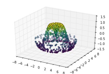
This leaves a lot to be desired. The function that will help us in this
case is ax.plot_trisurf, which creates a surface by first finding a
set of triangles formed between adjacent points (the result is shown in Figure 4-100; remember that x, y, and z here are one-dimensional arrays):
In[13]:ax=plt.axes(projection='3d')ax.plot_trisurf(x,y,z,cmap='viridis',edgecolor='none');
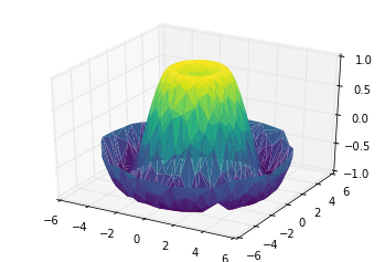
The result is certainly not as clean as when it is plotted with a grid, but the flexibility of such a triangulation allows for some really interesting three-dimensional plots. For example, it is actually possible to plot a three-dimensional Möbius strip using this, as we’ll see next.
A Möbius strip is similar to a strip of paper glued into a loop with a half-twist.
Topologically, it’s quite interesting because despite appearances it has
only a single side! Here we will visualize such an object using
Matplotlib’s three-dimensional tools. The key to creating the Möbius strip is to think
about its parameterization: it’s a two-dimensional strip, so we need two
intrinsic dimensions. Let’s call them  , which ranges
from 0 to
, which ranges
from 0 to  around the loop, and
 which ranges from –1 to 1 across the width of the strip:
In[14]:theta=np.linspace(0,2*np.pi,30)w=np.linspace(-0.25,0.25,8)w,theta=np.meshgrid(w,theta)
Now from this parameterization, we must determine the (x, y, z) positions of the embedded strip.
Thinking about it, we might realize that there are two rotations
happening: one is the position of the loop about its center (what we’ve
called  ), while the other is the twisting of the
strip about its axis (we’ll call this
), while the other is the twisting of the
strip about its axis (we’ll call this  ). For a Möbius
strip, we must have the strip make half a twist during a full loop, or
). For a Möbius
strip, we must have the strip make half a twist during a full loop, or
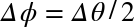 .
.
In[15]:phi=0.5*theta
Now we use our recollection of trigonometry to derive the
three-dimensional embedding. We’ll define  , the distance
of each point from the center, and use this to find the embedded
, the distance
of each point from the center, and use this to find the embedded
 coordinates:
In[16]:# radius in x-y planer=1+w*np.cos(phi)x=np.ravel(r*np.cos(theta))y=np.ravel(r*np.sin(theta))z=np.ravel(w*np.sin(phi))
Finally, to plot the object, we must make sure the triangulation is correct. The best way to do this is to define the triangulation within the underlying parameterization, and then let Matplotlib project this triangulation into the three-dimensional space of the Möbius strip. This can be accomplished as follows (Figure 4-101):
In[17]:# triangulate in the underlying parameterizationfrommatplotlib.triimportTriangulationtri=Triangulation(np.ravel(w),np.ravel(theta))ax=plt.axes(projection='3d')ax.plot_trisurf(x,y,z,triangles=tri.triangles,cmap='viridis',linewidths=0.2);ax.set_xlim(-1,1);ax.set_ylim(-1,1);ax.set_zlim(-1,1);
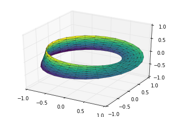
Combining all of these techniques, it is possible to create and display a wide variety of three-dimensional objects and patterns in Matplotlib.
One common type of visualization in data science is that of geographic
data. Matplotlib’s main tool for this type of visualization is the
Basemap toolkit, which is one of several Matplotlib toolkits that
live under the mpl_toolkits namespace. Admittedly, Basemap feels a
bit clunky to use, and often even simple visualizations take much longer
to render than you might hope. More modern solutions, such as leaflet or
the Google Maps API, may be a better choice for more intensive map
visualizations. Still, Basemap is a useful tool for Python users to
have in their virtual toolbelts. In this section, we’ll show several
examples of the type of map visualization that is possible with this
toolkit.
Installation of Basemap is straightforward; if you’re using conda you can type this and the package will be downloaded:
$ conda install basemap
We add just a single new import to our standard boilerplate:
In[1]:%matplotlibinlineimportnumpyasnpimportmatplotlib.pyplotaspltfrommpl_toolkits.basemapimportBasemap
Once you have the Basemap toolkit installed and imported, geographic
plots are just a few lines away (the graphics in Figure 4-102 also
require the PIL package in Python 2, or the pillow package in
Python 3):
In[2]:plt.figure(figsize=(8,8))m=Basemap(projection='ortho',resolution=None,lat_0=50,lon_0=-100)m.bluemarble(scale=0.5);

The meaning of the arguments to Basemap will be discussed momentarily.
The useful thing is that the globe shown here is not a mere image; it is a fully functioning Matplotlib axes that understands spherical coordinates and allows us to easily over-plot data on the map! For example, we can use a different map projection, zoom in to North America, and plot the location of Seattle. We’ll use an etopo image (which shows topographical features both on land and under the ocean) as the map background (Figure 4-103):
In[3]:fig=plt.figure(figsize=(8,8))m=Basemap(projection='lcc',resolution=None,width=8E6,height=8E6,lat_0=45,lon_0=-100,)m.etopo(scale=0.5,alpha=0.5)# Map (long, lat) to (x, y) for plottingx,y=m(-122.3,47.6)plt.plot(x,y,'ok',markersize=5)plt.text(x,y,' Seattle',fontsize=12);

This gives you a brief glimpse into the sort of geographic visualizations that are possible with just a few lines of Python. We’ll now discuss the features of Basemap in more depth, and provide several examples of visualizing map data. Using these brief examples as building blocks, you should be able to create nearly any map visualization that you desire.
The first thing to decide when you are using maps is which projection to use. You’re probably familiar with the fact that it is impossible to project a spherical map, such as that of the Earth, onto a flat surface without somehow distorting it or breaking its continuity. These projections have been developed over the course of human history, and there are a lot of choices! Depending on the intended use of the map projection, there are certain map features (e.g., direction, area, distance, shape, or other considerations) that are useful to maintain.
The Basemap package implements several dozen such projections, all referenced by a short format code. Here we’ll briefly demonstrate some of the more common ones.
We’ll start by defining a convenience routine to draw our world map along with the longitude and latitude lines:
In[4]:fromitertoolsimportchaindefdraw_map(m,scale=0.2):# draw a shaded-relief imagem.shadedrelief(scale=scale)# lats and longs are returned as a dictionarylats=m.drawparallels(np.linspace(-90,90,13))lons=m.drawmeridians(np.linspace(-180,180,13))# keys contain the plt.Line2D instanceslat_lines=chain(*(tup[1][0]fortupinlats.items()))lon_lines=chain(*(tup[1][0]fortupinlons.items()))all_lines=chain(lat_lines,lon_lines)# cycle through these lines and set the desired styleforlineinall_lines:line.set(linestyle='-',alpha=0.3,color='w')
The simplest of map projections are cylindrical projections, in which
lines of constant latitude and longitude are mapped to horizontal and
vertical lines, respectively. This type of mapping represents equatorial
regions quite well, but results in extreme distortions near the poles.
The spacing of latitude lines varies between different cylindrical
projections, leading to different conservation properties, and different
distortion near the poles. In Figure 4-104, we show an example of the equidistant
cylindrical projection, which chooses a latitude scaling that
preserves distances along meridians. Other cylindrical projections are
the Mercator (projection='merc') and the cylindrical equal-area
(projection='cea') projections.
In[5]:fig=plt.figure(figsize=(8,6),edgecolor='w')m=Basemap(projection='cyl',resolution=None,llcrnrlat=-90,urcrnrlat=90,llcrnrlon=-180,urcrnrlon=180,)draw_map(m)

The additional arguments to Basemap for this view specify the latitude
(lat) and longitude (lon) of the lower-left corner (llcrnr) and
upper-right corner (urcrnr) for the desired map, in units of degrees.
Pseudo-cylindrical projections relax the requirement that meridians
(lines of constant longitude) remain vertical; this can give better
properties near the poles of the projection. The Mollweide projection
(projection='moll') is one common example of this, in which all
meridians are elliptical arcs (Figure 4-105). It is constructed so as to preserve area
across the map: though there are distortions near the poles, the area of
small patches reflects the true area. Other pseudo-cylindrical
projections are the sinusoidal (projection='sinu') and Robinson
(projection='robin') projections.
In[6]:fig=plt.figure(figsize=(8,6),edgecolor='w')m=Basemap(projection='moll',resolution=None,lat_0=0,lon_0=0)draw_map(m)

The extra arguments to Basemap here refer to the central latitude
(lat_0) and longitude (lon_0) for the desired map.
Perspective projections are constructed using a particular choice of
perspective point, similar to if you photographed the Earth from a
particular point in space (a point which, for some projections,
technically lies within the Earth!). One common example is the
orthographic projection (projection='ortho'), which shows one side of
the globe as seen from a viewer at a very long distance. Thus, it can
show only half the globe at a time. Other perspective-based projections
include the gnomonic projection (projection='gnom') and stereographic
projection (projection='stere'). These are often the most useful for
showing small portions of the map.
Here is an example of the orthographic projection (Figure 4-106):
In[7]:fig=plt.figure(figsize=(8,8))m=Basemap(projection='ortho',resolution=None,lat_0=50,lon_0=0)draw_map(m);

A conic projection projects the map onto a single cone, which is then
unrolled. This can lead to very good local properties, but regions far
from the focus point of the cone may become very distorted. One example
of this is the Lambert conformal conic projection (projection='lcc'),
which we saw earlier in the map of North America. It projects the map onto
a cone arranged in such a way that two standard parallels (specified in
Basemap by lat_1 and lat_2) have well-represented distances, with
scale decreasing between them and increasing outside of them. Other
useful conic projections are the equidistant conic (projection='eqdc')
and the Albers equal-area (projection='aea') projection (Figure 4-107). Conic
projections, like perspective projections, tend to be good choices for
representing small to medium patches of the globe.
In[8]:fig=plt.figure(figsize=(8,8))m=Basemap(projection='lcc',resolution=None,lon_0=0,lat_0=50,lat_1=45,lat_2=55,width=1.6E7,height=1.2E7)draw_map(m)

If you’re going to do much with map-based visualizations, I encourage you to read up on other available projections, along with their properties, advantages, and disadvantages. Most likely, they are available in the Basemap package. If you dig deep enough into this topic, you’ll find an incredible subculture of geo-viz geeks who will be ready to argue fervently in support of their favorite projection for any given application!
Earlier we saw the bluemarble() and shadedrelief() methods
for projecting global images on the map, as well as the
drawparallels() and drawmeridians() methods for drawing lines of
constant latitude and longitude. The Basemap package contains a range of
useful functions for drawing borders of physical features like
continents, oceans, lakes, and rivers, as well as political boundaries
such as countries and US states and counties. The following are some of
the available drawing functions that you may wish to explore using
IPython’s help features:
Physical boundaries and bodies of water
drawcoastlines()Draw continental coast lines
drawlsmask()Draw a mask between the land and sea, for use with projecting images on one or the other
drawmapboundary()Draw the map boundary, including the fill color for oceans
drawrivers()Draw rivers on the map
fillcontinents()Fill the continents with a given color; optionally fill lakes with another color
Political boundaries
drawcountries()Draw country boundaries
drawstates()Draw US state boundaries
drawcounties()Draw US county boundaries
Map features
drawgreatcircle()Draw a great circle between two points
drawparallels()Draw lines of constant latitude
drawmeridians()Draw lines of constant longitude
drawmapscale()Draw a linear scale on the map
Whole-globe images
bluemarble()Project NASA’s blue marble image onto the map
shadedrelief()Project a shaded relief image onto the map
etopo()Draw an etopo relief image onto the map
warpimage()Project a user-provided image onto the map
For the boundary-based features, you must set the desired resolution
when creating a Basemap image. The resolution argument of the
Basemap class sets the level of detail in boundaries, either 'c'
(crude), 'l' (low), 'i' (intermediate), 'h' (high), 'f' (full),
or None if no boundaries will be used. This choice is important:
setting high-resolution boundaries on a global map, for example, can be
very slow.
Here’s an example of drawing land/sea boundaries, and the effect of the resolution parameter. We’ll create both a low- and high-resolution map of Scotland’s beautiful Isle of Skye. It’s located at 57.3°N, 6.2°W, and a map of 90,000×120,000 kilometers shows it well (Figure 4-108):
In[9]:fig,ax=plt.subplots(1,2,figsize=(12,8))fori,resinenumerate(['l','h']):m=Basemap(projection='gnom',lat_0=57.3,lon_0=-6.2,width=90000,height=120000,resolution=res,ax=ax[i])m.fillcontinents(color="#FFDDCC",lake_color='#DDEEFF')m.drawmapboundary(fill_color="#DDEEFF")m.drawcoastlines()ax[i].set_title("resolution='{0}'".format(res));
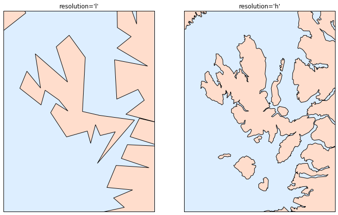
Notice that the low-resolution coastlines are not suitable for this level of zoom, while high-resolution works just fine. The low level would work just fine for a global view, however, and would be much faster than loading the high-resolution border data for the entire globe! It might require some experimentation to find the correct resolution parameter for a given view; the best route is to start with a fast, low-resolution plot and increase the resolution as needed.
Perhaps the most useful piece of the Basemap toolkit is the ability to
over-plot a variety of data onto a map background. For simple plotting
and text, any plt function works on the map; you can use the Basemap
instance to project latitude and longitude coordinates to (x, y)
coordinates for plotting with plt, as we saw earlier in the Seattle example.
In addition to this, there are many map-specific functions available
as methods of the Basemap instance. These work very similarly to their
standard Matplotlib counterparts, but have an additional Boolean
argument latlon, which if set to True allows you to pass raw
latitudes and longitudes to the method, rather than projected (x, y)
coordinates.
Some of these map-specific methods are:
contour()/contourf()Draw contour lines or filled contours
imshow()Draw an image
pcolor()/pcolormesh()Draw a pseudocolor plot for irregular/regular meshes
plot()Draw lines and/or markers
scatter()Draw points with markers
quiver()Draw vectors
barbs()Draw wind barbs
drawgreatcircle()Draw a great circle
We’ll see examples of a few of these as we continue. For more information on these functions, including several example plots, see the online Basemap documentation.
Recall that in “Customizing Plot Legends”, we demonstrated the use of size and color in a scatter plot to convey information about the location, size, and population of California cities. Here, we’ll create this plot again, but using Basemap to put the data in context.
We start with loading the data, as we did before:
In[10]:importpandasaspdcities=pd.read_csv('data/california_cities.csv')# Extract the data we're interested inlat=cities['latd'].valueslon=cities['longd'].valuespopulation=cities['population_total'].valuesarea=cities['area_total_km2'].values
Next, we set up the map projection, scatter the data, and then create a colorbar and legend (Figure 4-109):
In[11]:# 1. Draw the map backgroundfig=plt.figure(figsize=(8,8))m=Basemap(projection='lcc',resolution='h',lat_0=37.5,lon_0=-119,width=1E6,height=1.2E6)m.shadedrelief()m.drawcoastlines(color='gray')m.drawcountries(color='gray')m.drawstates(color='gray')# 2. scatter city data, with color reflecting population# and size reflecting aream.scatter(lon,lat,latlon=True,c=np.log10(population),s=area,cmap='Reds',alpha=0.5)# 3. create colorbar and legendplt.colorbar(label=r'$\log_{10}({\rm population})$')plt.clim(3,7)# make legend with dummy pointsforain[100,300,500]:plt.scatter([],[],c='k',alpha=0.5,s=a,label=str(a)+' km$^2$')plt.legend(scatterpoints=1,frameon=False,labelspacing=1,loc='lower left');
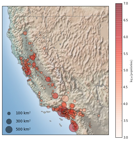
This shows us roughly where larger populations of people have settled in California: they are clustered near the coast in the Los Angeles and San Francisco areas, stretched along the highways in the flat central valley, and avoiding almost completely the mountainous regions along the borders of the state.
As an example of visualizing some more continuous geographic data, let’s consider the “polar vortex” that hit the eastern half of the United States in January 2014. A great source for any sort of climatic data is NASA’s Goddard Institute for Space Studies. Here we’ll use the GIS 250 temperature data, which we can download using shell commands (these commands may have to be modified on Windows machines). The data used here was downloaded on 6/12/2016, and the file size is approximately 9 MB:
In[12]:# !curl -O http://data.giss.nasa.gov/pub/gistemp/gistemp250.nc.gz# !gunzip gistemp250.nc.gz
The data comes in NetCDF format, which can be read in Python by the
netCDF4 library. You can install this library as shown here:
$ conda install netcdf4
We read the data as follows:
In[13]:fromnetCDF4importDatasetdata=Dataset('gistemp250.nc')
The file contains many global temperature readings on a variety of dates; we need to select the index of the date we’re interested in—in this case, January 15, 2014:
In[14]:fromnetCDF4importdate2indexfromdatetimeimportdatetimetimeindex=date2index(datetime(2014,1,15),data.variables['time'])
Now we can load the latitude and longitude data, as well as the temperature anomaly for this index:
In[15]:lat=data.variables['lat'][:]lon=data.variables['lon'][:]lon,lat=np.meshgrid(lon,lat)temp_anomaly=data.variables['tempanomaly'][timeindex]
Finally, we’ll use the pcolormesh() method to draw a color mesh of the
data. We’ll look at North America, and use a shaded relief map in the
background. Note that for this data we specifically chose a divergent
colormap, which has a neutral color at zero and two contrasting colors
at negative and positive values (Figure 4-110). We’ll also lightly draw the coastlines
over the colors for reference:
In[16]:fig=plt.figure(figsize=(10,8))m=Basemap(projection='lcc',resolution='c',width=8E6,height=8E6,lat_0=45,lon_0=-100,)m.shadedrelief(scale=0.5)m.pcolormesh(lon,lat,temp_anomaly,latlon=True,cmap='RdBu_r')plt.clim(-8,8)m.drawcoastlines(color='lightgray')plt.title('January 2014 Temperature Anomaly')plt.colorbar(label='temperature anomaly (°C)');
The data paints a picture of the localized, extreme temperature anomalies that happened during that month. The eastern half of the United States was much colder than normal, while the western half and Alaska were much warmer. Regions with no recorded temperature show the map background.
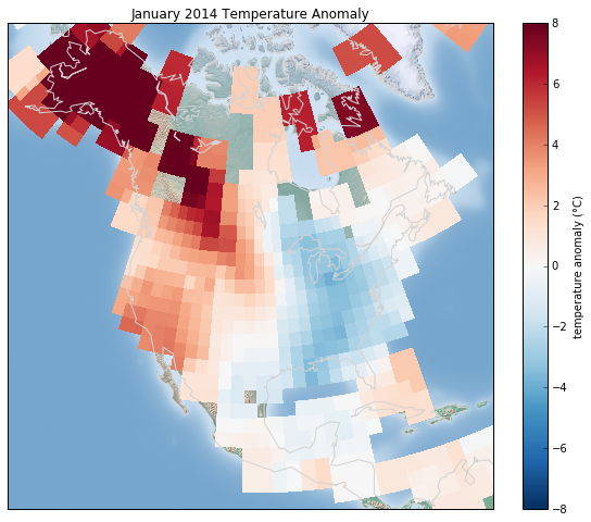
Matplotlib has proven to be an incredibly useful and popular visualization tool, but even avid users will admit it often leaves much to be desired. There are several valid complaints about Matplotlib that often come up:
Prior to version 2.0, Matplotlib’s defaults are not exactly the best choices. It was based off of MATLAB circa 1999, and this often shows.
Matplotlib’s API is relatively low level. Doing sophisticated statistical visualization is possible, but often requires a lot of boilerplate code.
Matplotlib predated Pandas by more than a decade, and thus is not
designed for use with Pandas DataFrames. In order to visualize data from
a Pandas DataFrame, you must extract each Series and often concatenate
them together into the right format. It would be nicer to have
a plotting library that can intelligently use the DataFrame labels in a
plot.
An answer to these problems is
Seaborn. Seaborn
provides an API on top of Matplotlib that offers sane choices for plot
style and color defaults, defines simple high-level functions for common
statistical plot types, and integrates with the functionality
provided by Pandas DataFrames.
To be fair, the Matplotlib team is addressing this: it has recently
added the plt.style tools (discussed in
“Customizing Matplotlib: Configurations and Stylesheets”), and is starting to handle Pandas data
more seamlessly. The 2.0 release of the library will include a new
default stylesheet that will improve on the current status quo. But for
all the reasons just discussed, Seaborn remains an extremely useful
add-on.
Here is an example of a simple random-walk plot in Matplotlib, using its classic plot formatting and colors. We start with the typical imports:
In[1]:importmatplotlib.pyplotaspltplt.style.use('classic')%matplotlibinlineimportnumpyasnpimportpandasaspd
Now we create some random walk data:
In[2]:# Create some datarng=np.random.RandomState(0)x=np.linspace(0,10,500)y=np.cumsum(rng.randn(500,6),0)
And do a simple plot (Figure 4-111):
In[3]:# Plot the data with Matplotlib defaultsplt.plot(x,y)plt.legend('ABCDEF',ncol=2,loc='upper left');
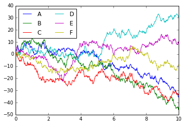
Although the result contains all the information we’d like it to convey, it does so in a way that is not all that aesthetically pleasing, and even looks a bit old-fashioned in the context of 21st-century data visualization.
Now let’s take a look at how it works with Seaborn. As we will see, Seaborn has many of its
own high-level plotting routines, but it can also overwrite Matplotlib’s default parameters and in turn get even simple Matplotlib scripts to produce vastly superior output.
We can set the style by calling Seaborn’s set() method. By convention,
Seaborn is imported as sns:
In[4]:importseabornassnssns.set()
Now let’s rerun the same two lines as before (Figure 4-112):
In[5]:# same plotting code as above!plt.plot(x,y)plt.legend('ABCDEF',ncol=2,loc='upper left');
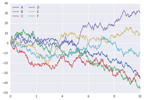
The main idea of Seaborn is that it provides high-level commands to create a variety of plot types useful for statistical data exploration, and even some statistical model fitting.
Let’s take a look at a few of the datasets and plot types available in Seaborn. Note that all of the following could be done using raw Matplotlib commands (this is, in fact, what Seaborn does under the hood), but the Seaborn API is much more convenient.
Often in statistical data visualization, all you want is to plot histograms and joint distributions of variables. We have seen that this is relatively straightforward in Matplotlib (Figure 4-113):
In[6]:data=np.random.multivariate_normal([0,0],[[5,2],[2,2]],size=2000)data=pd.DataFrame(data,columns=['x','y'])forcolin'xy':plt.hist(data[col],normed=True,alpha=0.5)
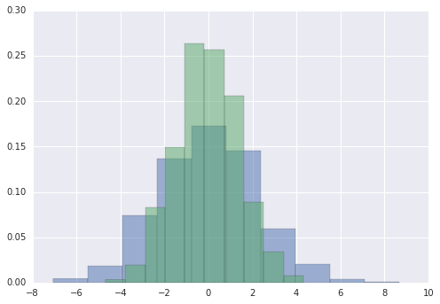
Rather than a histogram, we can get a smooth estimate of the
distribution using a kernel density estimation, which Seaborn does with
sns.kdeplot (Figure 4-114):
In[7]:forcolin'xy':sns.kdeplot(data[col],shade=True)
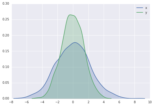
Histograms and KDE can be combined using distplot (Figure 4-115):
In[8]:sns.distplot(data['x'])sns.distplot(data['y']);
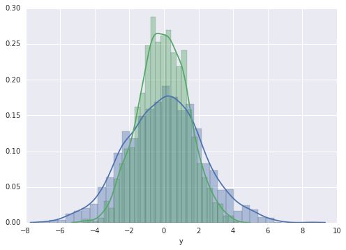
If we pass the full two-dimensional dataset to kdeplot, we will get a
two-dimensional visualization of the data (Figure 4-116):
In[9]:sns.kdeplot(data);
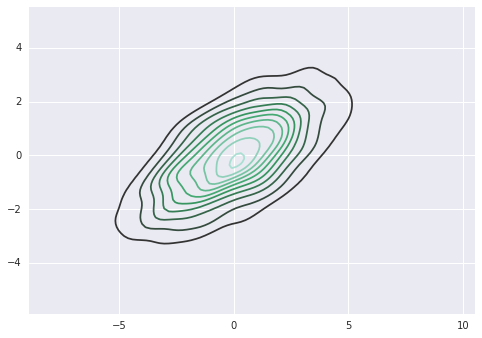
We can see the joint distribution and the marginal distributions
together using sns.jointplot. For this plot, we’ll set the style to a
white background (Figure 4-117):
In[10]:withsns.axes_style('white'):sns.jointplot("x","y",data,kind='kde');
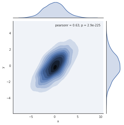
There are other parameters that can be passed to jointplot—for
example, we can use a hexagonally based histogram instead (Figure 4-118):
In[11]:withsns.axes_style('white'):sns.jointplot("x","y",data,kind='hex')
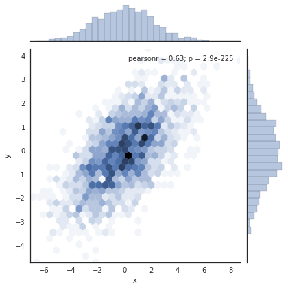
When you generalize joint plots to datasets of larger dimensions, you end up with pair plots. This is very useful for exploring correlations between multidimensional data, when you’d like to plot all pairs of values against each other.
We’ll demo this with the well-known Iris dataset, which lists measurements of petals and sepals of three iris species:
In[12]:iris=sns.load_dataset("iris")iris.head()
Out[12]: sepal_length sepal_width petal_length petal_width species
0 5.1 3.5 1.4 0.2 setosa
1 4.9 3.0 1.4 0.2 setosa
2 4.7 3.2 1.3 0.2 setosa
3 4.6 3.1 1.5 0.2 setosa
4 5.0 3.6 1.4 0.2 setosa
Visualizing the multidimensional relationships among the samples is as
easy as calling sns.pairplot (Figure 4-119):
In[13]:sns.pairplot(iris,hue='species',size=2.5);
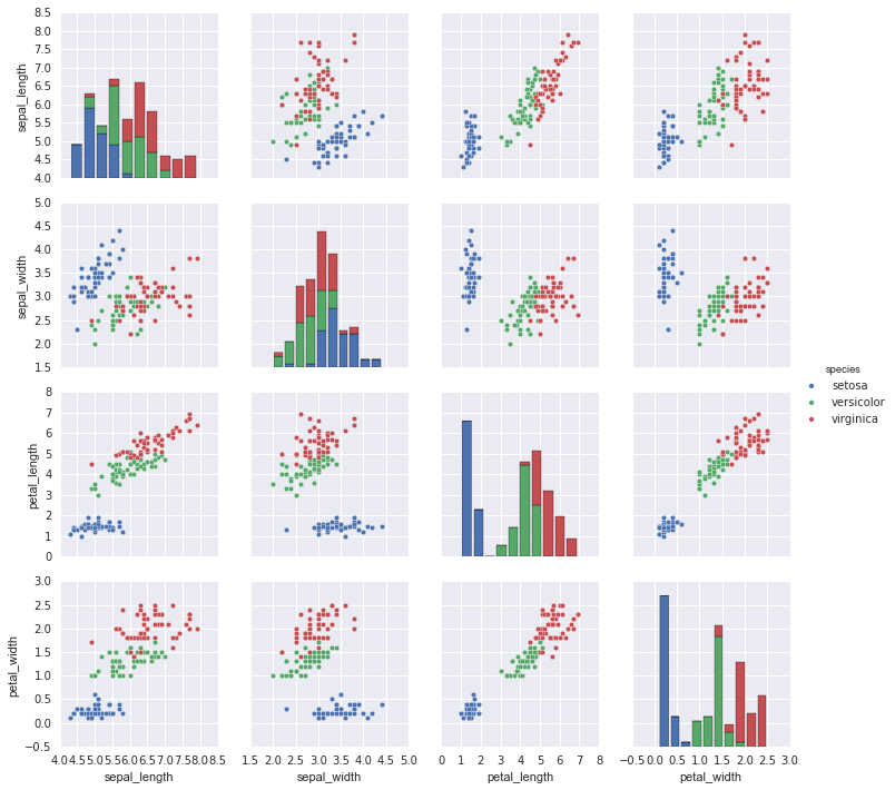
Sometimes the best way to view data is via histograms of subsets.
Seaborn’s FacetGrid makes this extremely simple. We’ll take a look at
some data that shows the amount that restaurant staff receive in tips
based on various indicator data (Figure 4-120):
In[14]:tips=sns.load_dataset('tips')tips.head()
Out[14]: total_bill tip sex smoker day time size
0 16.99 1.01 Female No Sun Dinner 2
1 10.34 1.66 Male No Sun Dinner 3
2 21.01 3.50 Male No Sun Dinner 3
3 23.68 3.31 Male No Sun Dinner 2
4 24.59 3.61 Female No Sun Dinner 4
In[15]:tips['tip_pct']=100*tips['tip']/tips['total_bill']grid=sns.FacetGrid(tips,row="sex",col="time",margin_titles=True)grid.map(plt.hist,"tip_pct",bins=np.linspace(0,40,15));
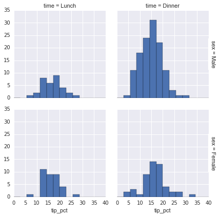
Factor plots can be useful for this kind of visualization as well. This allows you to view the distribution of a parameter within bins defined by any other parameter (Figure 4-121):
In[16]:withsns.axes_style(style='ticks'):g=sns.factorplot("day","total_bill","sex",data=tips,kind="box")g.set_axis_labels("Day","Total Bill");
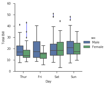
Similar to the pair plot we saw earlier, we can use sns.jointplot to show
the joint distribution between different datasets, along with the
associated marginal distributions (Figure 4-122):
In[17]:withsns.axes_style('white'):sns.jointplot("total_bill","tip",data=tips,kind='hex')
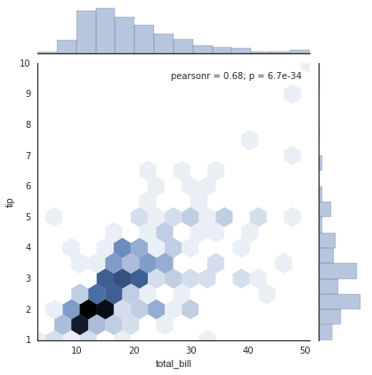
The joint plot can even do some automatic kernel density estimation and regression (Figure 4-123):
In[18]:sns.jointplot("total_bill","tip",data=tips,kind='reg');
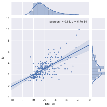
Time series can be plotted with sns.factorplot. In the following example (visualized in Figure 4-124), we’ll use the Planets data that we first saw in
“Aggregation and Grouping”:
In[19]:planets=sns.load_dataset('planets')planets.head()
Out[19]: method number orbital_period mass distance year
0 Radial Velocity 1 269.300 7.10 77.40 2006
1 Radial Velocity 1 874.774 2.21 56.95 2008
2 Radial Velocity 1 763.000 2.60 19.84 2011
3 Radial Velocity 1 326.030 19.40 110.62 2007
4 Radial Velocity 1 516.220 10.50 119.47 2009
In[20]:withsns.axes_style('white'):g=sns.factorplot("year",data=planets,aspect=2,kind="count",color='steelblue')g.set_xticklabels(step=5)
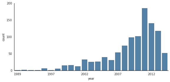
We can learn more by looking at the method of discovery of each of these planets, as illustrated in Figure 4-125:
In[21]:withsns.axes_style('white'):g=sns.factorplot("year",data=planets,aspect=4.0,kind='count',hue='method',order=range(2001,2015))g.set_ylabels('Number of Planets Discovered')
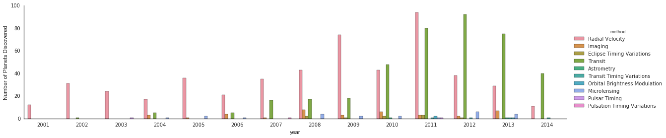
For more information on plotting with Seaborn, see the Seaborn documentation, a tutorial, and the Seaborn gallery.
Here we’ll look at using Seaborn to help visualize and understand finishing results from a marathon. I’ve scraped the data from sources on the Web, aggregated it and removed any identifying information, and put it on GitHub where it can be downloaded (if you are interested in using Python for web scraping, I would recommend Web Scraping with Python by Ryan Mitchell). We will start by downloading the data from the Web, and loading it into Pandas:
In[22]:# !curl -O https://raw.githubusercontent.com/jakevdp/marathon-data/# master/marathon-data.csv
In[23]:data=pd.read_csv('marathon-data.csv')data.head()
Out[23]: age gender split final
0 33 M 01:05:38 02:08:51
1 32 M 01:06:26 02:09:28
2 31 M 01:06:49 02:10:42
3 38 M 01:06:16 02:13:45
4 31 M 01:06:32 02:13:59
By default, Pandas loaded the time columns as Python strings (type
object); we can see this by looking at the dtypes attribute of the
DataFrame:
In[24]:data.dtypes
Out[24]: age int64
gender object
split object
final object
dtype: object
Let’s fix this by providing a converter for the times:
In[25]:defconvert_time(s):h,m,s=map(int,s.split(':'))returnpd.datetools.timedelta(hours=h,minutes=m,seconds=s)data=pd.read_csv('marathon-data.csv',converters={'split':convert_time,'final':convert_time})data.head()
Out[25]: age gender split final
0 33 M 01:05:38 02:08:51
1 32 M 01:06:26 02:09:28
2 31 M 01:06:49 02:10:42
3 38 M 01:06:16 02:13:45
4 31 M 01:06:32 02:13:59
In[26]:data.dtypes
Out[26]: age int64
gender object
split timedelta64[ns]
final timedelta64[ns]
dtype: object
That looks much better. For the purpose of our Seaborn plotting utilities, let’s next add columns that give the times in seconds:
In[27]:data['split_sec']=data['split'].astype(int)/1E9data['final_sec']=data['final'].astype(int)/1E9data.head()
Out[27]: age gender split final split_sec final_sec
0 33 M 01:05:38 02:08:51 3938.0 7731.0
1 32 M 01:06:26 02:09:28 3986.0 7768.0
2 31 M 01:06:49 02:10:42 4009.0 7842.0
3 38 M 01:06:16 02:13:45 3976.0 8025.0
4 31 M 01:06:32 02:13:59 3992.0 8039.0
To get an idea of what the data looks like, we can plot a jointplot
over the data (Figure 4-126):
In[28]:withsns.axes_style('white'):g=sns.jointplot("split_sec","final_sec",data,kind='hex')g.ax_joint.plot(np.linspace(4000,16000),np.linspace(8000,32000),':k')
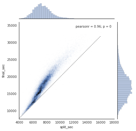
The dotted line shows where someone’s time would lie if they ran the marathon at a perfectly steady pace. The fact that the distribution lies above this indicates (as you might expect) that most people slow down over the course of the marathon. If you have run competitively, you’ll know that those who do the opposite—run faster during the second half of the race—are said to have “negative-split” the race.
Let’s create another column in the data, the split fraction, which measures the degree to which each runner negative-splits or positive-splits the race:
In[29]:data['split_frac']=1-2*data['split_sec']/data['final_sec']data.head()
Out[29]: age gender split final split_sec final_sec split_frac
0 33 M 01:05:38 02:08:51 3938.0 7731.0 -0.018756
1 32 M 01:06:26 02:09:28 3986.0 7768.0 -0.026262
2 31 M 01:06:49 02:10:42 4009.0 7842.0 -0.022443
3 38 M 01:06:16 02:13:45 3976.0 8025.0 0.009097
4 31 M 01:06:32 02:13:59 3992.0 8039.0 0.006842
Where this split difference is less than zero, the person negative-split the race by that fraction. Let’s do a distribution plot of this split fraction (Figure 4-127):
In[30]:sns.distplot(data['split_frac'],kde=False);plt.axvline(0,color="k",linestyle="--");
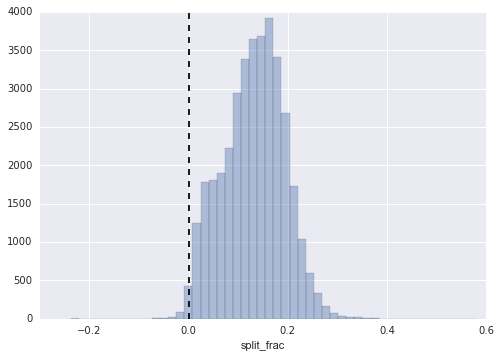
In[31]:sum(data.split_frac<0)
Out[31]: 251
Out of nearly 40,000 participants, there were only 250 people who negative-split their marathon.
Let’s see whether there is any correlation between this split fraction
and other variables. We’ll do this using a pairgrid, which draws plots
of all these correlations (Figure 4-128):
In[32]:g=sns.PairGrid(data,vars=['age','split_sec','final_sec','split_frac'],hue='gender',palette='RdBu_r')g.map(plt.scatter,alpha=0.8)g.add_legend();
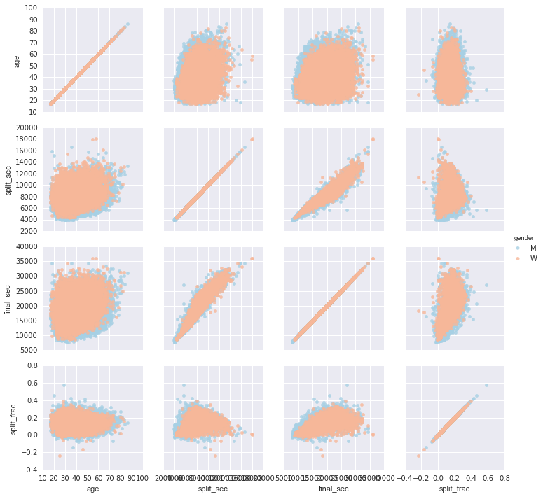
It looks like the split fraction does not correlate particularly with age, but does correlate with the final time: faster runners tend to have closer to even splits on their marathon time. (We see here that Seaborn is no panacea for Matplotlib’s ills when it comes to plot styles: in particular, the x-axis labels overlap. Because the output is a simple Matplotlib plot, however, the methods in “Customizing Ticks” can be used to adjust such things if desired.)
The difference between men and women here is interesting. Let’s look at the histogram of split fractions for these two groups (Figure 4-129):
In[33]:sns.kdeplot(data.split_frac[data.gender=='M'],label='men',shade=True)sns.kdeplot(data.split_frac[data.gender=='W'],label='women',shade=True)plt.xlabel('split_frac');
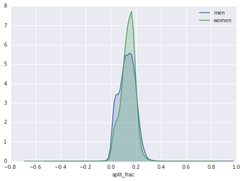
The interesting thing here is that there are many more men than women who are running close to an even split! This almost looks like some kind of bimodal distribution among the men and women. Let’s see if we can suss out what’s going on by looking at the distributions as a function of age.
A nice way to compare distributions is to use a violin plot (Figure 4-130):
In[34]:sns.violinplot("gender","split_frac",data=data,palette=["lightblue","lightpink"]);
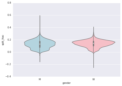
This is yet another way to compare the distributions between men and women.
Let’s look a little deeper, and compare these violin plots as a function of age. We’ll start by creating a new column in the array that specifies the decade of age that each person is in (Figure 4-131):
In[35]:data['age_dec']=data.age.map(lambdaage:10*(age//10))data.head()
Out[35]: age gender split final split_sec final_sec split_frac age_dec 0 33 M 01:05:38 02:08:51 3938.0 7731.0 -0.018756 30 1 32 M 01:06:26 02:09:28 3986.0 7768.0 -0.026262 30 2 31 M 01:06:49 02:10:42 4009.0 7842.0 -0.022443 30 3 38 M 01:06:16 02:13:45 3976.0 8025.0 0.009097 30 4 31 M 01:06:32 02:13:59 3992.0 8039.0 0.006842 30
In[36]:men=(data.gender=='M')women=(data.gender=='W')withsns.axes_style(style=None):sns.violinplot("age_dec","split_frac",hue="gender",data=data,split=True,inner="quartile",palette=["lightblue","lightpink"]);
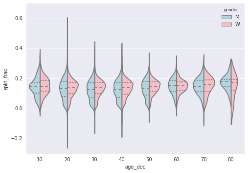
Looking at this, we can see where the distributions of men and women differ: the split distributions of men in their 20s to 50s show a pronounced over-density toward lower splits when compared to women of the same age (or of any age, for that matter).
Also surprisingly, the 80-year-old women seem to outperform everyone in terms of their split time. This is probably due to the fact that we’re estimating the distribution from small numbers, as there are only a handful of runners in that range:
In[38]:(data.age>80).sum()
Out[38]: 7
Back to the men with negative splits: who are these runners? Does this
split fraction correlate with finishing quickly? We can plot this very
easily. We’ll use regplot, which will automatically fit a linear
regression to the data (Figure 4-132):
In[37]:g=sns.lmplot('final_sec','split_frac',col='gender',data=data,markers=".",scatter_kws=dict(color='c'))g.map(plt.axhline,y=0.1,color="k",ls=":");
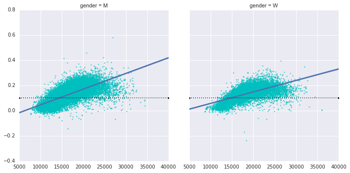
Apparently the people with fast splits are the elite runners who are finishing within ~15,000 seconds, or about 4 hours. People slower than that are much less likely to have a fast second split.
A single chapter in a book can never hope to cover all the available features and plot types available in Matplotlib. As with other packages we’ve seen, liberal use of IPython’s tab-completion and help functions (see “Help and Documentation in IPython”) can be very helpful when you’re exploring Matplotlib’s API. In addition, Matplotlib’s online documentation can be a helpful reference. See in particular the Matplotlib gallery linked on that page: it shows thumbnails of hundreds of different plot types, each one linked to a page with the Python code snippet used to generate it. In this way, you can visually inspect and learn about a wide range of different plotting styles and visualization techniques.
For a book-length treatment of Matplotlib, I would recommend Interactive Applications Using Matplotlib, written by Matplotlib core developer Ben Root.
Although Matplotlib is the most prominent Python visualization library, there are other more modern tools that are worth exploring as well. I’ll mention a few of them briefly here:
Bokeh is a JavaScript visualization library with a Python frontend that creates highly interactive visualizations capable of handling very large and/or streaming datasets. The Python frontend outputs a JSON data structure that can be interpreted by the Bokeh JS engine.
Plotly is the eponymous open source product of the Plotly company, and is similar in spirit to Bokeh. Because Plotly is the main product of a startup, it is receiving a high level of development effort. Use of the library is entirely free.
Vispy is an actively developed project focused on dynamic visualizations of very large datasets. Because it is built to target OpenGL and make use of efficient graphics processors in your computer, it is able to render some quite large and stunning visualizations.
Vega and Vega-Lite are declarative graphics representations, and are the product of years of research into the fundamental language of data visualization. The reference rendering implementation is JavaScript, but the API is language agnostic. There is a Python API under development in the Altair package. Though it’s not mature yet, I’m quite excited for the possibilities of this project to provide a common reference point for visualization in Python and other languages.
The visualization space in the Python community is very dynamic, and I fully expect this list to be out of date as soon as it is published. Keep an eye out for what’s coming in the future!
In many ways, machine learning is the primary means by which data science manifests itself to the broader world. Machine learning is where these computational and algorithmic skills of data science meet the statistical thinking of data science, and the result is a collection of approaches to inference and data exploration that are not about effective theory so much as effective computation.
The term “machine learning” is sometimes thrown around as if it is some kind of magic pill: apply machine learning to your data, and all your problems will be solved! As you might expect, the reality is rarely this simple. While these methods can be incredibly powerful, to be effective they must be approached with a firm grasp of the strengths and weaknesses of each method, as well as a grasp of general concepts such as bias and variance, overfitting and underfitting, and more.
This chapter will dive into practical aspects of machine learning, primarily using Python’s Scikit-Learn package. This is not meant to be a comprehensive introduction to the field of machine learning; that is a large subject and necessitates a more technical approach than we take here. Nor is it meant to be a comprehensive manual for the use of the Scikit-Learn package (for this, see “Further Machine Learning Resources”). Rather, the goals of this chapter are:
To introduce the fundamental vocabulary and concepts of machine learning.
To introduce the Scikit-Learn API and show some examples of its use.
To take a deeper dive into the details of several of the most important machine learning approaches, and develop an intuition into how they work and when and where they are applicable.
Much of this material is drawn from the Scikit-Learn tutorials and workshops I have given on several occasions at PyCon, SciPy, PyData, and other conferences. Any clarity in the following pages is likely due to the many workshop participants and co-instructors who have given me valuable feedback on this material over the years!
Finally, if you are seeking a more comprehensive or technical treatment of any of these subjects, I’ve listed several resources and references in “Further Machine Learning Resources”.
Before we take a look at the details of various machine learning methods, let’s start by looking at what machine learning is, and what it isn’t. Machine learning is often categorized as a subfield of artificial intelligence, but I find that categorization can often be misleading at first brush. The study of machine learning certainly arose from research in this context, but in the data science application of machine learning methods, it’s more helpful to think of machine learning as a means of building models of data.
Fundamentally, machine learning involves building mathematical models to help understand data. “Learning” enters the fray when we give these models tunable parameters that can be adapted to observed data; in this way the program can be considered to be “learning” from the data. Once these models have been fit to previously seen data, they can be used to predict and understand aspects of newly observed data. I’ll leave to the reader the more philosophical digression regarding the extent to which this type of mathematical, model-based “learning” is similar to the “learning” exhibited by the human brain.
Understanding the problem setting in machine learning is essential to using these tools effectively, and so we will start with some broad categorizations of the types of approaches we’ll discuss here.
At the most fundamental level, machine learning can be categorized into two main types: supervised learning and unsupervised learning.
Supervised learning involves somehow modeling the relationship between measured features of data and some label associated with the data; once this model is determined, it can be used to apply labels to new, unknown data. This is further subdivided into classification tasks and regression tasks: in classification, the labels are discrete categories, while in regression, the labels are continuous quantities. We will see examples of both types of supervised learning in the following section.
Unsupervised learning involves modeling the features of a dataset without reference to any label, and is often described as “letting the dataset speak for itself.” These models include tasks such as clustering and dimensionality reduction. Clustering algorithms identify distinct groups of data, while dimensionality reduction algorithms search for more succinct representations of the data. We will see examples of both types of unsupervised learning in the following section.
In addition, there are so-called semi-supervised learning methods, which fall somewhere between supervised learning and unsupervised learning. Semi-supervised learning methods are often useful when only incomplete labels are available.
To make these ideas more concrete, let’s take a look at a few very simple examples of a machine learning task. These examples are meant to give an intuitive, non-quantitative overview of the types of machine learning tasks we will be looking at in this chapter. In later sections, we will go into more depth regarding the particular models and how they are used. For a preview of these more technical aspects, you can find the Python source that generates the figures in the online appendix.
We will first take a look at a simple classification task, in which you are given a set of labeled points and want to use these to classify some unlabeled points.
Imagine that we have the data shown in Figure 5-1 (the code used to generate this figure, and all figures in this section, is available in the online appendix).
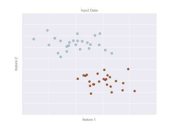
Here we have two-dimensional data; that is, we have two features for each point, represented by the (x,y) positions of the points on the plane. In addition, we have one of two class labels for each point, here represented by the colors of the points. From these features and labels, we would like to create a model that will let us decide whether a new point should be labeled “blue” or “red.”
There are a number of possible models for such a classification task, but here we will use an extremely simple one. We will make the assumption that the two groups can be separated by drawing a straight line through the plane between them, such that points on each side of the line fall in the same group. Here the model is a quantitative version of the statement “a straight line separates the classes,” while the model parameters are the particular numbers describing the location and orientation of that line for our data. The optimal values for these model parameters are learned from the data (this is the “learning” in machine learning), which is often called training the model.
Figure 5-2 is a visual representation of what the trained model looks like for this data.
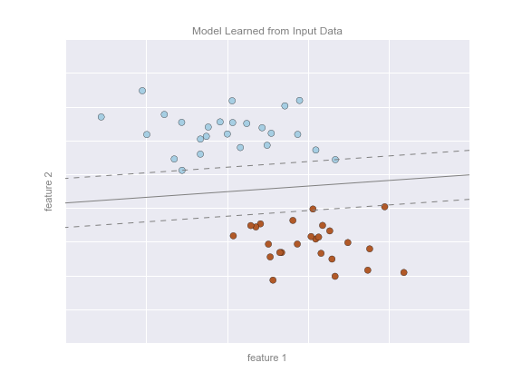
Now that this model has been trained, it can be generalized to new, unlabeled data. In other words, we can take a new set of data, draw this model line through it, and assign labels to the new points based on this model. This stage is usually called prediction. See Figure 5-3.
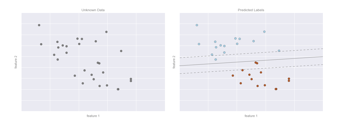
This is the basic idea of a classification task in machine learning, where “classification” indicates that the data has discrete class labels. At first glance this may look fairly trivial: it would be relatively easy to simply look at this data and draw such a discriminatory line to accomplish this classification. A benefit of the machine learning approach, however, is that it can generalize to much larger datasets in many more dimensions.
For example, this is similar to the task of automated spam detection for email; in this case, we might use the following features and labels:
feature 1, feature 2, etc.  normalized counts of
important words or phrases (“Viagra,” “Nigerian prince,” etc.)
normalized counts of
important words or phrases (“Viagra,” “Nigerian prince,” etc.)
label  “spam” or “not spam”
For the training set, these labels might be determined by individual inspection of a small representative sample of emails; for the remaining emails, the label would be determined using the model. For a suitably trained classification algorithm with enough well-constructed features (typically thousands or millions of words or phrases), this type of approach can be very effective. We will see an example of such text-based classification in “In Depth: Naive Bayes Classification”.
Some important classification algorithms that we will discuss in more detail are Gaussian naive Bayes (see “In Depth: Naive Bayes Classification”), support vector machines (see “In-Depth: Support Vector Machines”), and random forest classification (see “In-Depth: Decision Trees and Random Forests”).
In contrast with the discrete labels of a classification algorithm, we will next look at a simple regression task in which the labels are continuous quantities.
Consider the data shown in Figure 5-4, which consists of a set of points, each with a continuous label.
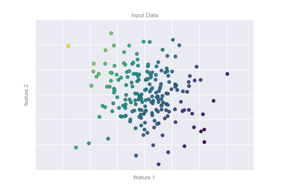
As with the classification example, we have two-dimensional data; that is, there are two features describing each data point. The color of each point represents the continuous label for that point.
There are a number of possible regression models we might use for this type of data, but here we will use a simple linear regression to predict the points. This simple linear regression model assumes that if we treat the label as a third spatial dimension, we can fit a plane to the data. This is a higher-level generalization of the well-known problem of fitting a line to data with two coordinates.
We can visualize this setup as shown in Figure 5-5.
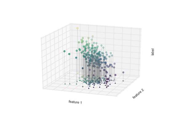
Notice that the feature 1–feature 2 plane here is the same as in the two-dimensional plot from before; in this case, however, we have represented the labels by both color and three-dimensional axis position. From this view, it seems reasonable that fitting a plane through this three-dimensional data would allow us to predict the expected label for any set of input parameters. Returning to the two-dimensional projection, when we fit such a plane we get the result shown in Figure 5-6.
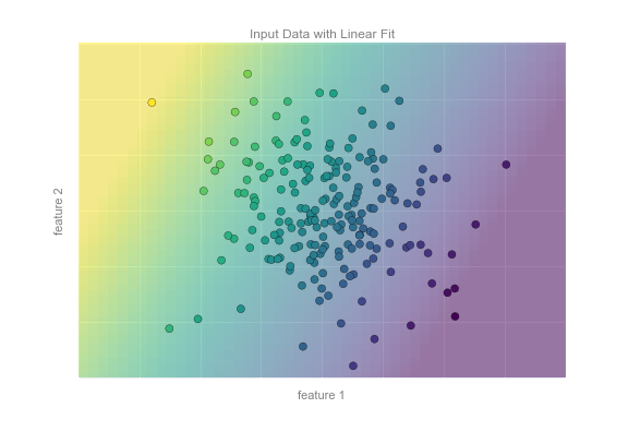
This plane of fit gives us what we need to predict labels for new points. Visually, we find the results shown in Figure 5-7.
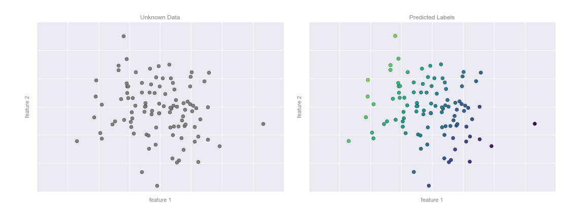
As with the classification example, this may seem rather trivial in a low number of dimensions. But the power of these methods is that they can be straightforwardly applied and evaluated in the case of data with many, many features.
For example, this is similar to the task of computing the distance to galaxies observed through a telescope—in this case, we might use the following features and labels:
feature 1, feature 2, etc.  brightness of each
galaxy at one of several wavelengths or colors
brightness of each
galaxy at one of several wavelengths or colors
label  distance or redshift of the galaxy
The distances for a small number of these galaxies might be determined through an independent set of (typically more expensive) observations. We could then estimate distances to remaining galaxies using a suitable regression model, without the need to employ the more expensive observation across the entire set. In astronomy circles, this is known as the “photometric redshift” problem.
Some important regression algorithms that we will discuss are linear regression (see “In Depth: Linear Regression”), support vector machines (see “In-Depth: Support Vector Machines”), and random forest regression (see “In-Depth: Decision Trees and Random Forests”).
The classification and regression illustrations we just looked at are examples of supervised learning algorithms, in which we are trying to build a model that will predict labels for new data. Unsupervised learning involves models that describe data without reference to any known labels.
One common case of unsupervised learning is “clustering,” in which data is automatically assigned to some number of discrete groups. For example, we might have some two-dimensional data like that shown in Figure 5-8.
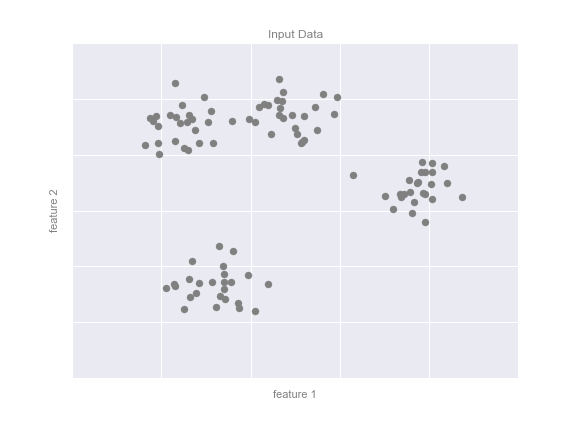
By eye, it is clear that each of these points is part of a distinct group. Given this input, a clustering model will use the intrinsic structure of the data to determine which points are related. Using the very fast and intuitive k-means algorithm (see “In Depth: k-Means Clustering”), we find the clusters shown in Figure 5-9.
k-means fits a model consisting of k cluster centers; the optimal centers are assumed to be those that minimize the distance of each point from its assigned center. Again, this might seem like a trivial exercise in two dimensions, but as our data becomes larger and more complex, such clustering algorithms can be employed to extract useful information from the dataset.
We will discuss the k-means algorithm in more depth in “In Depth: k-Means Clustering”. Other important clustering algorithms include Gaussian mixture models (see “In Depth: Gaussian Mixture Models”) and spectral clustering (see Scikit-Learn’s clustering documentation).
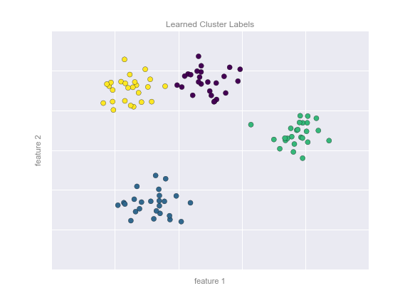
Dimensionality reduction is another example of an unsupervised algorithm, in which labels or other information are inferred from the structure of the dataset itself. Dimensionality reduction is a bit more abstract than the examples we looked at before, but generally it seeks to pull out some low-dimensional representation of data that in some way preserves relevant qualities of the full dataset. Different dimensionality reduction routines measure these relevant qualities in different ways, as we will see in “In-Depth: Manifold Learning”.
As an example of this, consider the data shown in Figure 5-10.
Visually, it is clear that there is some structure in this data: it is drawn from a one-dimensional line that is arranged in a spiral within this two-dimensional space. In a sense, you could say that this data is “intrinsically” only one dimensional, though this one-dimensional data is embedded in higher-dimensional space. A suitable dimensionality reduction model in this case would be sensitive to this nonlinear embedded structure, and be able to pull out this lower-dimensionality representation.
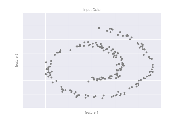
Figure 5-11 presents a visualization of the results of the Isomap algorithm, a manifold learning algorithm that does exactly this.
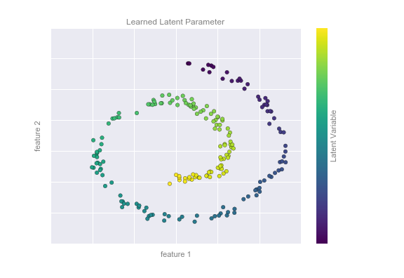
Notice that the colors (which represent the extracted one-dimensional latent variable) change uniformly along the spiral, which indicates that the algorithm did in fact detect the structure we saw by eye. As with the previous examples, the power of dimensionality reduction algorithms becomes clearer in higher-dimensional cases. For example, we might wish to visualize important relationships within a dataset that has 100 or 1,000 features. Visualizing 1,000-dimensional data is a challenge, and one way we can make this more manageable is to use a dimensionality reduction technique to reduce the data to two or three dimensions.
Some important dimensionality reduction algorithms that we will discuss are principal component analysis (see “In Depth: Principal Component Analysis”) and various manifold learning algorithms, including Isomap and locally linear embedding (see “In-Depth: Manifold Learning”).
Here we have seen a few simple examples of some of the basic types of machine learning approaches. Needless to say, there are a number of important practical details that we have glossed over, but I hope this section was enough to give you a basic idea of what types of problems machine learning approaches can solve.
In short, we saw the following:
Models that can predict labels based on labeled training data
Models that predict labels as two or more discrete categories
Models that predict continuous labels
Models that identify structure in unlabeled data
Models that detect and identify distinct groups in the data
Models that detect and identify lower-dimensional structure in higher-dimensional data
In the following sections we will go into much greater depth within these categories, and see some more interesting examples of where these concepts can be useful.
All of the figures in the preceding discussion are generated based on actual machine learning computations; the code behind them can be found in the online appendix.
There are several Python libraries that provide solid implementations of a range of machine learning algorithms. One of the best known is Scikit-Learn, a package that provides efficient versions of a large number of common algorithms. Scikit-Learn is characterized by a clean, uniform, and streamlined API, as well as by very useful and complete online documentation. A benefit of this uniformity is that once you understand the basic use and syntax of Scikit-Learn for one type of model, switching to a new model or algorithm is very straightforward.
This section provides an overview of the Scikit-Learn API; a solid understanding of these API elements will form the foundation for understanding the deeper practical discussion of machine learning algorithms and approaches in the following chapters.
We will start by covering data representation in Scikit-Learn, followed by covering the Estimator API, and finally go through a more interesting example of using these tools for exploring a set of images of handwritten digits.
Machine learning is about creating models from data: for that reason, we’ll start by discussing how data can be represented in order to be understood by the computer. The best way to think about data within Scikit-Learn is in terms of tables of data.
A basic table is a two-dimensional grid of data, in which the rows
represent individual elements of the dataset, and the columns represent
quantities related to each of these elements. For example, consider the
Iris dataset,
famously analyzed by Ronald Fisher in 1936. We can download this dataset in the form of a Pandas DataFrame using the Seaborn library:
In[1]:importseabornassnsiris=sns.load_dataset('iris')iris.head()
Out[1]: sepal_length sepal_width petal_length petal_width species
0 5.1 3.5 1.4 0.2 setosa
1 4.9 3.0 1.4 0.2 setosa
2 4.7 3.2 1.3 0.2 setosa
3 4.6 3.1 1.5 0.2 setosa
4 5.0 3.6 1.4 0.2 setosa
Here each row of the data refers to a single observed flower, and the
number of rows is the total number of flowers in the dataset. In
general, we will refer to the rows of the matrix as samples, and the
number of rows as n_samples.
Likewise, each column of the data refers to a particular quantitative
piece of information that describes each sample. In general, we will
refer to the columns of the matrix as features, and the number of
columns as n_features.
This table layout makes clear that the information can be thought of as
a two-dimensional numerical array or matrix, which we will call the
features matrix. By convention, this features matrix is often stored
in a variable named X. The features matrix is assumed to be
two-dimensional, with shape [n_samples, n_features], and is most often
contained in a NumPy array or a Pandas DataFrame, though some Scikit-Learn
models also accept SciPy sparse matrices.
The samples (i.e., rows) always refer to the individual objects described by the dataset. For example, the sample might be a flower, a person, a document, an image, a sound file, a video, an astronomical object, or anything else you can describe with a set of quantitative measurements.
The features (i.e., columns) always refer to the distinct observations that describe each sample in a quantitative manner. Features are generally real-valued, but may be Boolean or discrete-valued in some cases.
In addition to the feature matrix X, we also generally work with a
label or target array, which by convention we will usually call y.
The target array is usually one dimensional, with length n_samples,
and is generally contained in a NumPy array or Pandas Series. The target
array may have continuous numerical values, or discrete classes/labels.
While some Scikit-Learn estimators do handle multiple target values in
the form of a two-dimensional [n_samples, n_targets] target array, we
will primarily be working with the common case of a one-dimensional
target array.
Often one point of confusion is how the target array differs from the
other features columns. The distinguishing feature of the target array
is that it is usually the quantity we want to predict from the data:
in statistical terms, it is the dependent variable. For example, in the
preceding data we may wish to construct a model that can predict the species
of flower based on the other measurements; in this case, the species
column would be considered the feature.
With this target array in mind, we can use Seaborn (discussed earlier in “Visualization with Seaborn”) to conveniently visualize the data (see Figure 5-12):
In[2]:%matplotlibinlineimportseabornassns;sns.set()sns.pairplot(iris,hue='species',size=1.5);
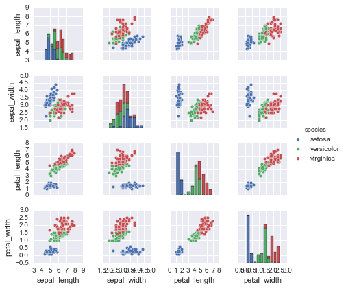
For use in Scikit-Learn, we will extract the features matrix and target
array from the DataFrame, which we can do using some of the Pandas
DataFrame operations discussed in Chapter 3:
In[3]:X_iris=iris.drop('species',axis=1)X_iris.shape
Out[3]: (150, 4)
In[4]:y_iris=iris['species']y_iris.shape
Out[4]: (150,)
To summarize, the expected layout of features and target values is visualized in Figure 5-13.
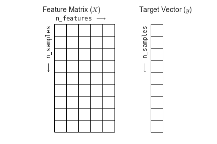
With this data properly formatted, we can move on to consider the estimator API of Scikit-Learn.
The Scikit-Learn API is designed with the following guiding principles in mind, as outlined in the Scikit-Learn API paper:
All objects share a common interface drawn from a limited set of methods, with consistent documentation.
All specified parameter values are exposed as public attributes.
Only algorithms are represented by Python
classes; datasets are represented in standard formats (NumPy arrays,
Pandas DataFrames, SciPy sparse matrices) and parameter names use
standard Python strings.
Many machine learning tasks can be expressed as sequences of more fundamental algorithms, and Scikit-Learn makes use of this wherever possible.
When models require user-specified parameters, the library defines an appropriate default value.
In practice, these principles make Scikit-Learn very easy to use, once the basic principles are understood. Every machine learning algorithm in Scikit-Learn is implemented via the Estimator API, which provides a consistent interface for a wide range of machine learning applications.
Most commonly, the steps in using the Scikit-Learn estimator API are as follows (we will step through a handful of detailed examples in the sections that follow):
Choose a class of model by importing the appropriate estimator class from Scikit-Learn.
Choose model hyperparameters by instantiating this class with desired values.
Arrange data into a features matrix and target vector following the discussion from before.
Fit the model to your data by calling the fit() method of the
model instance.
Apply the model to new data:
For supervised learning, often we predict labels for unknown data
using the predict() method.
For unsupervised learning, we often transform or infer properties of
the data using the transform() or predict() method.
We will now step through several simple examples of applying supervised and unsupervised learning methods.
As an example of this process, let’s consider a simple linear regression—that is, the common case of fitting a line to  data. We will use the following simple data for our regression example (Figure 5-14):
In[5]:importmatplotlib.pyplotaspltimportnumpyasnprng=np.random.RandomState(42)x=10*rng.rand(50)y=2*x-1+rng.randn(50)plt.scatter(x,y);
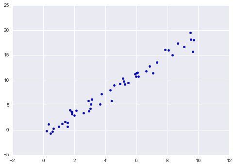
With this data in place, we can use the recipe outlined earlier. Let’s walk through the process:
Choose a class of model.
In Scikit-Learn, every class of model is represented by a Python class. So, for example, if we would like to compute a simple linear regression model, we can import the linear regression class:
In[6]:fromsklearn.linear_modelimportLinearRegression
Note that other, more general linear regression models exist as well; you
can read more about them in the
sklearn.linear_model
module documentation.
Choose model hyperparameters.
An important point is that a class of model is not the same as an instance of a model.
Once we have decided on our model class, there are still some options open to us. Depending on the model class we are working with, we might need to answer one or more questions like the following:
Would we like to fit for the offset (i.e., intercept)?
Would we like the model to be normalized?
Would we like to preprocess our features to add model flexibility?
What degree of regularization would we like to use in our model?
How many model components would we like to use?
These are examples of the important choices that must be made once the model class is selected. These choices are often represented as hyperparameters, or parameters that must be set before the model is fit to data. In Scikit-Learn, we choose hyperparameters by passing values at model instantiation. We will explore how you can quantitatively motivate the choice of hyperparameters in “Hyperparameters and Model Validation”.
For our linear regression example, we can instantiate the
LinearRegression class and specify that we would like to fit the
intercept using the fit_intercept hyperparameter:
In[7]:model=LinearRegression(fit_intercept=True)model
Out[7]: LinearRegression(copy_X=True, fit_intercept=True, n_jobs=1,
normalize=False)
Keep in mind that when the model is instantiated, the only action is the storing of these hyperparameter values. In particular, we have not yet applied the model to any data: the Scikit-Learn API makes very clear the distinction between choice of model and application of model to data.
Arrange data into a features matrix and target vector.
Previously we detailed the Scikit-Learn data representation, which
requires a two-dimensional features matrix and a one-dimensional target
array. Here our target variable y is already in the correct form (a
length-n_samples array), but we need to massage the data x to make
it a matrix of size [n_samples, n_features]. In this case, this
amounts to a simple reshaping of the one-dimensional array:
In[8]:X=x[:,np.newaxis]X.shape
Out[8]: (50, 1)
Fit the model to your data.
Now it is time to apply our model to data. This can be done with the
fit() method of the model:
In[9]:model.fit(X,y)
Out[9]:
LinearRegression(copy_X=True, fit_intercept=True, n_jobs=1,
normalize=False)
This fit() command causes a number of model-dependent internal
computations to take place, and the results of these computations are
stored in model-specific attributes that the user can explore. In
Scikit-Learn, by convention all model parameters that were learned
during the fit() process have trailing underscores; for example, in
this linear model, we have the following:
In[10]:model.coef_
Out[10]: array([ 1.9776566])
In[11]:model.intercept_
Out[11]: -0.90331072553111635
These two parameters represent the slope and intercept of the simple linear fit to the data. Comparing to the data definition, we see that they are very close to the input slope of 2 and intercept of –1.
One question that frequently comes up regards the uncertainty in such internal model parameters. In general, Scikit-Learn does not provide tools to draw conclusions from internal model parameters themselves: interpreting model parameters is much more a statistical modeling question than a machine learning question. Machine learning rather focuses on what the model predicts. If you would like to dive into the meaning of fit parameters within the model, other tools are available, including the StatsModels Python package.
Predict labels for unknown data.
Once the model is trained, the main task of supervised machine learning
is to evaluate it based on what it says about new data that was not
part of the training set. In Scikit-Learn, we can do this using the
predict() method. For the sake of this example, our “new data” will be
a grid of x values, and we will ask what y values the model predicts:
In[12]:xfit=np.linspace(-1,11)
As before, we need to coerce these x values into a
[n_samples, n_features] features matrix, after which we can feed it to
the model:
In[13]:Xfit=xfit[:,np.newaxis]yfit=model.predict(Xfit)
Finally, let’s visualize the results by plotting first the raw data, and then this model fit (Figure 5-15):
In[14]:plt.scatter(x,y)plt.plot(xfit,yfit);
Typically one evaluates the efficacy of the model by comparing its results to some known baseline, as we will see in the next example.
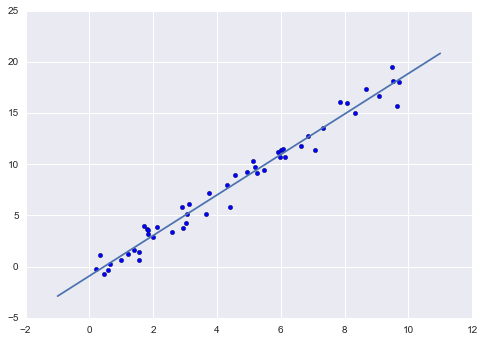
Let’s take a look at another example of this process, using the Iris dataset we discussed earlier. Our question will be this: given a model trained on a portion of the Iris data, how well can we predict the remaining labels?
For this task, we will use an extremely simple generative model known as Gaussian naive Bayes, which proceeds by assuming each class is drawn from an axis-aligned Gaussian distribution (see “In Depth: Naive Bayes Classification” for more details). Because it is so fast and has no hyperparameters to choose, Gaussian naive Bayes is often a good model to use as a baseline classification, before you explore whether improvements can be found through more sophisticated models.
We would like to evaluate the model on data it has not seen before, and
so we will split the data into a training set and a testing set.
This could be done by hand, but it is more convenient to use the
train_test_split utility function:
In[15]:fromsklearn.cross_validationimporttrain_test_splitXtrain,Xtest,ytrain,ytest=train_test_split(X_iris,y_iris,random_state=1)
With the data arranged, we can follow our recipe to predict the labels:
In[16]:fromsklearn.naive_bayesimportGaussianNB# 1. choose model classmodel=GaussianNB()# 2. instantiate modelmodel.fit(Xtrain,ytrain)# 3. fit model to datay_model=model.predict(Xtest)# 4. predict on new data
Finally, we can use the accuracy_score utility to see the fraction of
predicted labels that match their true value:
In[17]:fromsklearn.metricsimportaccuracy_scoreaccuracy_score(ytest,y_model)
Out[17]: 0.97368421052631582
With an accuracy topping 97%, we see that even this very naive classification algorithm is effective for this particular dataset!
As an example of an unsupervised learning problem, let’s take a look at reducing the dimensionality of the Iris data so as to more easily visualize it. Recall that the Iris data is four dimensional: there are four features recorded for each sample.
The task of dimensionality reduction is to ask whether there is a suitable lower-dimensional representation that retains the essential features of the data. Often dimensionality reduction is used as an aid to visualizing data; after all, it is much easier to plot data in two dimensions than in four dimensions or higher!
Here we will use principal component analysis (PCA; see “In Depth: Principal Component Analysis”), which is a fast linear dimensionality reduction technique. We will ask the model to return two components—that is, a two-dimensional representation of the data.
Following the sequence of steps outlined earlier, we have:
In[18]:fromsklearn.decompositionimportPCA# 1. Choose the model classmodel=PCA(n_components=2)# 2. Instantiate the model with hyperparametersmodel.fit(X_iris)# 3. Fit to data. Notice y is not specified!X_2D=model.transform(X_iris)# 4. Transform the data to two dimensions
Now let’s plot the results. A quick way to do this is to insert the
results into the original Iris DataFrame, and use Seaborn’s lmplot to
show the results (Figure 5-16):
In[19]:iris['PCA1']=X_2D[:,0]iris['PCA2']=X_2D[:,1]sns.lmplot("PCA1","PCA2",hue='species',data=iris,fit_reg=False);
We see that in the two-dimensional representation, the species are fairly well separated, even though the PCA algorithm had no knowledge of the species labels! This indicates to us that a relatively straightforward classification will probably be effective on the dataset, as we saw before.
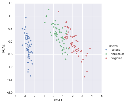
Let’s next look at applying clustering to the Iris data. A clustering algorithm attempts to find distinct groups of data without reference to any labels. Here we will use a powerful clustering method called a Gaussian mixture model (GMM), discussed in more detail in “In Depth: Gaussian Mixture Models”. A GMM attempts to model the data as a collection of Gaussian blobs.
We can fit the Gaussian mixture model as follows:
In[20]:fromsklearn.mixtureimportGMM# 1. Choose the model classmodel=GMM(n_components=3,covariance_type='full')# 2. Instantiate the model w/ hyperparametersmodel.fit(X_iris)# 3. Fit to data. Notice y is not specified!y_gmm=model.predict(X_iris)# 4. Determine cluster labels
As before, we will add the cluster label to the Iris DataFrame and use
Seaborn to plot the results (Figure 5-17):
In[21]:iris['cluster']=y_gmmsns.lmplot("PCA1","PCA2",data=iris,hue='species',col='cluster',fit_reg=False);
By splitting the data by cluster number, we see exactly how well the GMM algorithm has recovered the underlying label: the setosa species is separated perfectly within cluster 0, while there remains a small amount of mixing between versicolor and virginica. This means that even without an expert to tell us the species labels of the individual flowers, the measurements of these flowers are distinct enough that we could automatically identify the presence of these different groups of species with a simple clustering algorithm! This sort of algorithm might further give experts in the field clues as to the relationship between the samples they are observing.
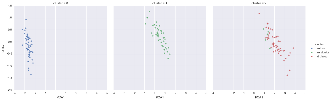
To demonstrate these principles on a more interesting problem, let’s consider one piece of the optical character recognition problem: the identification of handwritten digits. In the wild, this problem involves both locating and identifying characters in an image. Here we’ll take a shortcut and use Scikit-Learn’s set of preformatted digits, which is built into the library.
We’ll use Scikit-Learn’s data access interface and take a look at this data:
In[22]:fromsklearn.datasetsimportload_digitsdigits=load_digits()digits.images.shape
Out[22]: (1797, 8, 8)
The images data is a three-dimensional array: 1,797 samples, each consisting of an 8×8 grid of pixels. Let’s visualize the first hundred of these (Figure 5-18):
In[23]:importmatplotlib.pyplotaspltfig,axes=plt.subplots(10,10,figsize=(8,8),subplot_kw={'xticks':[],'yticks':[]},gridspec_kw=dict(hspace=0.1,wspace=0.1))fori,axinenumerate(axes.flat):ax.imshow(digits.images[i],cmap='binary',interpolation='nearest')ax.text(0.05,0.05,str(digits.target[i]),transform=ax.transAxes,color='green')
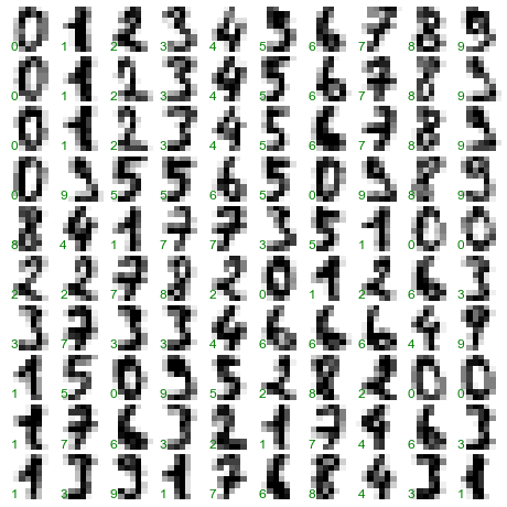
In order to work with this data within Scikit-Learn, we need a
two-dimensional, [n_samples, n_features] representation. We can
accomplish this by treating each pixel in the image as a feature—that
is, by flattening out the pixel arrays so that we have a length-64 array
of pixel values representing each digit. Additionally, we need the
target array, which gives the previously determined label for each
digit. These two quantities are built into the digits dataset under the
data and target attributes, respectively:
In[24]:X=digits.dataX.shape
Out[24]: (1797, 64)
In[25]:y=digits.targety.shape
Out[25]: (1797,)
We see here that there are 1,797 samples and 64 features.
We’d like to visualize our points within the 64-dimensional parameter space, but it’s difficult to effectively visualize points in such a high-dimensional space. Instead we’ll reduce the dimensions to 2, using an unsupervised method. Here, we’ll make use of a manifold learning algorithm called Isomap (see “In-Depth: Manifold Learning”), and transform the data to two dimensions:
In[26]:fromsklearn.manifoldimportIsomapiso=Isomap(n_components=2)iso.fit(digits.data)data_projected=iso.transform(digits.data)data_projected.shape
Out[26]: (1797, 2)
We see that the projected data is now two-dimensional. Let’s plot this data to see if we can learn anything from its structure (Figure 5-19):
In[27]:plt.scatter(data_projected[:,0],data_projected[:,1],c=digits.target,edgecolor='none',alpha=0.5,cmap=plt.cm.get_cmap('spectral',10))plt.colorbar(label='digit label',ticks=range(10))plt.clim(-0.5,9.5);
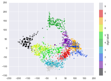
This plot gives us some good intuition into how well various numbers are separated in the larger 64-dimensional space. For example, zeros (in black) and ones (in purple) have very little overlap in parameter space. Intuitively, this makes sense: a zero is empty in the middle of the image, while a one will generally have ink in the middle. On the other hand, there seems to be a more or less continuous spectrum between ones and fours: we can understand this by realizing that some people draw ones with “hats” on them, which cause them to look similar to fours.
Overall, however, the different groups appear to be fairly well separated in the parameter space: this tells us that even a very straightforward supervised classification algorithm should perform suitably on this data. Let’s give it a try.
Let’s apply a classification algorithm to the digits. As with the Iris data previously, we will split the data into a training and test set, and fit a Gaussian naive Bayes model:
In[28]:Xtrain,Xtest,ytrain,ytest=train_test_split(X,y,random_state=0)
In[29]:fromsklearn.naive_bayesimportGaussianNBmodel=GaussianNB()model.fit(Xtrain,ytrain)y_model=model.predict(Xtest)
Now that we have predicted our model, we can gauge its accuracy by comparing the true values of the test set to the predictions:
In[30]:fromsklearn.metricsimportaccuracy_scoreaccuracy_score(ytest,y_model)
Out[30]: 0.83333333333333337
With even this extremely simple model, we find about 80% accuracy for classification of the digits! However, this single number doesn’t tell us where we’ve gone wrong—one nice way to do this is to use the confusion matrix, which we can compute with Scikit-Learn and plot with Seaborn (Figure 5-20):
In[31]:fromsklearn.metricsimportconfusion_matrixmat=confusion_matrix(ytest,y_model)sns.heatmap(mat,square=True,annot=True,cbar=False)plt.xlabel('predicted value')plt.ylabel('true value');
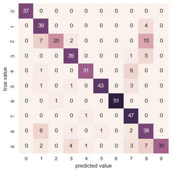
This shows us where the mislabeled points tend to be: for example, a large number of twos here are misclassified as either ones or eights. Another way to gain intuition into the characteristics of the model is to plot the inputs again, with their predicted labels. We’ll use green for correct labels, and red for incorrect labels (Figure 5-21):
In[32]:fig,axes=plt.subplots(10,10,figsize=(8,8),subplot_kw={'xticks':[],'yticks':[]},gridspec_kw=dict(hspace=0.1,wspace=0.1))fori,axinenumerate(axes.flat):ax.imshow(digits.images[i],cmap='binary',interpolation='nearest')ax.text(0.05,0.05,str(y_model[i]),transform=ax.transAxes,color='green'if(ytest[i]==y_model[i])else'red')
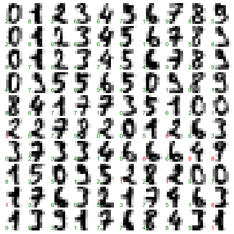
Examining this subset of the data, we can gain insight regarding where the algorithm might not be performing optimally. To go beyond our 80% classification rate, we might move to a more sophisticated algorithm, such as support vector machines (see “In-Depth: Support Vector Machines”) or random forests (see “In-Depth: Decision Trees and Random Forests”), or another classification approach.
In this section we have covered the essential features of the Scikit-Learn data representation, and the estimator API. Regardless of the type of estimator, the same import/instantiate/fit/predict pattern holds. Armed with this information about the estimator API, you can explore the Scikit-Learn documentation and begin trying out various models on your data.
In the next section, we will explore perhaps the most important topic in machine learning: how to select and validate your model.
In the previous section, we saw the basic recipe for applying a supervised machine learning model:
Choose a class of model
Choose model hyperparameters
Fit the model to the training data
Use the model to predict labels for new data
The first two pieces of this—the choice of model and choice of hyperparameters—are perhaps the most important part of using these tools and techniques effectively. In order to make an informed choice, we need a way to validate that our model and our hyperparameters are a good fit to the data. While this may sound simple, there are some pitfalls that you must avoid to do this effectively.
In principle, model validation is very simple: after choosing a model and its hyperparameters, we can estimate how effective it is by applying it to some of the training data and comparing the prediction to the known value.
The following sections first show a naive approach to model validation and why it fails, before exploring the use of holdout sets and cross-validation for more robust model evaluation.
Let’s demonstrate the naive approach to validation using the Iris data, which we saw in the previous section. We will start by loading the data:
In[1]:fromsklearn.datasetsimportload_irisiris=load_iris()X=iris.datay=iris.target
Next we choose a model and hyperparameters. Here we’ll use a k-neighbors
classifier with n_neighbors=1. This is a very simple and intuitive
model that says “the label of an unknown point is the same as the label
of its closest training point”:
In[2]:fromsklearn.neighborsimportKNeighborsClassifiermodel=KNeighborsClassifier(n_neighbors=1)
Then we train the model, and use it to predict labels for data we already know:
In[3]:model.fit(X,y)y_model=model.predict(X)
Finally, we compute the fraction of correctly labeled points:
In[4]:fromsklearn.metricsimportaccuracy_scoreaccuracy_score(y,y_model)
Out[4]: 1.0
We see an accuracy score of 1.0, which indicates that 100% of points were correctly labeled by our model! But is this truly measuring the expected accuracy? Have we really come upon a model that we expect to be correct 100% of the time?
As you may have gathered, the answer is no. In fact, this approach contains a fundamental flaw: it trains and evaluates the model on the same data. Furthermore, the nearest neighbor model is an instance-based estimator that simply stores the training data, and predicts labels by comparing new data to these stored points; except in contrived cases, it will get 100% accuracy every time!
So what can be done? We can get a better sense of a model’s performance using what’s known as a holdout set; that is, we hold back some
subset of the data from the training of the model, and then use this
holdout set to check the model performance. We can do this splitting using the train_test_split utility in Scikit-Learn:
In[5]:fromsklearn.cross_validationimporttrain_test_split# split the data with 50% in each setX1,X2,y1,y2=train_test_split(X,y,random_state=0,train_size=0.5)# fit the model on one set of datamodel.fit(X1,y1)# evaluate the model on the second set of datay2_model=model.predict(X2)accuracy_score(y2,y2_model)
Out[5]: 0.90666666666666662
We see here a more reasonable result: the nearest-neighbor classifier is about 90% accurate on this holdout set. The holdout set is similar to unknown data, because the model has not “seen” it before.
One disadvantage of using a holdout set for model validation is that we have lost a portion of our data to the model training. In the previous case, half the dataset does not contribute to the training of the model! This is not optimal, and can cause problems—especially if the initial set of training data is small.
One way to address this is to use cross-validation—that is, to do a sequence of fits where each subset of the data is used both as a training set and as a validation set. Visually, it might look something like Figure 5-22.
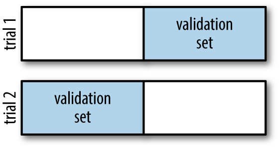
Here we do two validation trials, alternately using each half of the data as a holdout set. Using the split data from before, we could implement it like this:
In[6]:y2_model=model.fit(X1,y1).predict(X2)y1_model=model.fit(X2,y2).predict(X1)accuracy_score(y1,y1_model),accuracy_score(y2,y2_model)
Out[6]: (0.95999999999999996, 0.90666666666666662)
What comes out are two accuracy scores, which we could combine (by, say, taking the mean) to get a better measure of the global model performance. This particular form of cross-validation is a two-fold cross-validation—one in which we have split the data into two sets and used each in turn as a validation set.
We could expand on this idea to use even more trials, and more folds in the data—for example, Figure 5-23 is a visual depiction of five-fold cross-validation.
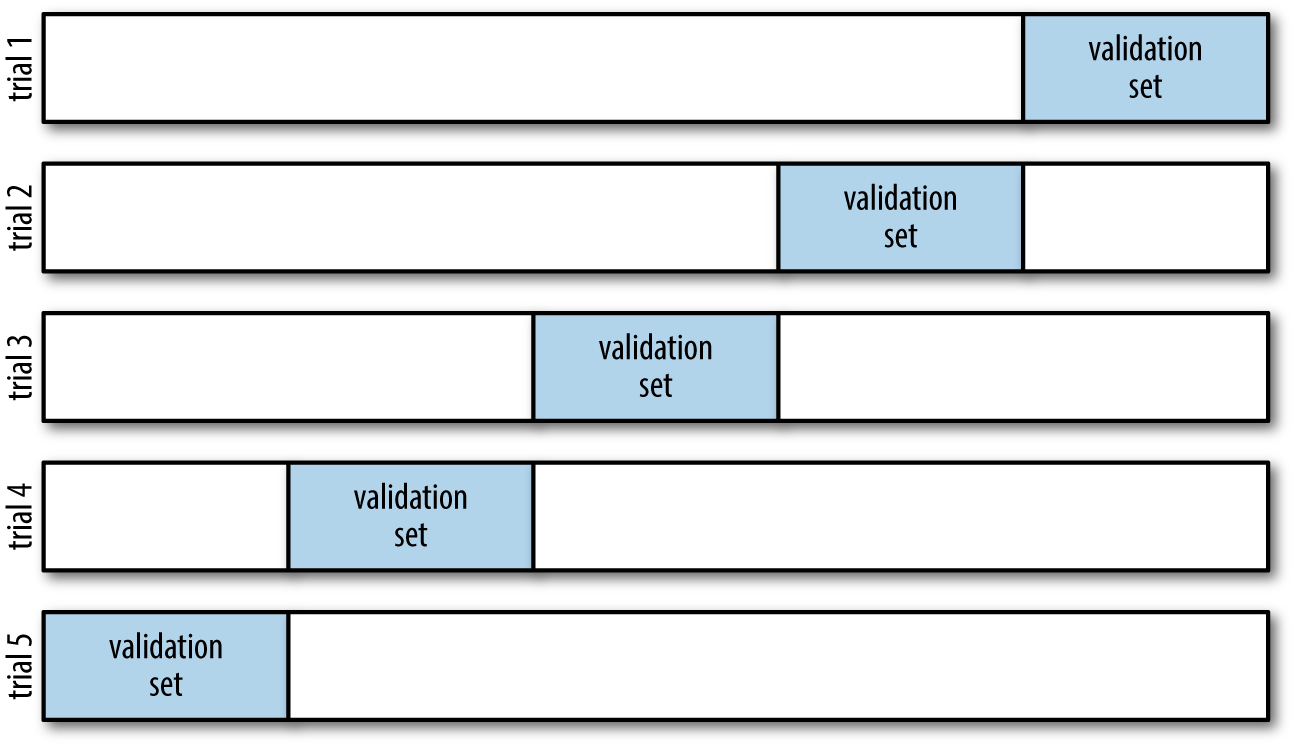
Here we split the data into five groups, and use each of them in turn to
evaluate the model fit on the other 4/5 of the data. This would be
rather tedious to do by hand, and so we can use Scikit-Learn’s
cross_val_score convenience routine to do it succinctly:
In[7]:fromsklearn.cross_validationimportcross_val_scorecross_val_score(model,X,y,cv=5)
Out[7]: array([ 0.96666667, 0.96666667, 0.93333333, 0.93333333, 1. ])
Repeating the validation across different subsets of the data gives us an even better idea of the performance of the algorithm.
Scikit-Learn implements a number of cross-validation schemes that
are useful in particular situations; these are implemented via iterators
in the cross_validation module. For example, we might wish to go to
the extreme case in which our number of folds is equal to the number of
data points; that is, we train on all points but one in each trial. This
type of cross-validation is known as leave-one-out cross-validation,
and can be used as follows:
In[8]:fromsklearn.cross_validationimportLeaveOneOutscores=cross_val_score(model,X,y,cv=LeaveOneOut(len(X)))scores
Out[8]: array([ 1., 1., 1., 1., 1., 1., 1., 1., 1., 1., 1., 1., 1.,
1., 1., 1., 1., 1., 1., 1., 1., 1., 1., 1., 1., 1.,
1., 1., 1., 1., 1., 1., 1., 1., 1., 1., 1., 1., 1.,
1., 1., 1., 1., 1., 1., 1., 1., 1., 1., 1., 1., 1.,
1., 1., 1., 1., 1., 1., 1., 1., 1., 1., 1., 1., 1.,
1., 1., 1., 1., 1., 0., 1., 0., 1., 1., 1., 1., 1.,
1., 1., 1., 1., 1., 0., 1., 1., 1., 1., 1., 1., 1.,
1., 1., 1., 1., 1., 1., 1., 1., 1., 1., 1., 1., 1.,
1., 1., 0., 1., 1., 1., 1., 1., 1., 1., 1., 1., 1.,
1., 1., 0., 1., 1., 1., 1., 1., 1., 1., 1., 1., 1.,
1., 1., 1., 0., 1., 1., 1., 1., 1., 1., 1., 1., 1.,
1., 1., 1., 1., 1., 1., 1.])
Because we have 150 samples, the leave-one-out cross-validation yields scores for 150 trials, and the score indicates either successful (1.0) or unsuccessful (0.0) prediction. Taking the mean of these gives an estimate of the error rate:
In[9]:scores.mean()
Out[9]: 0.95999999999999996
Other cross-validation schemes can be used similarly. For a description
of what is available in Scikit-Learn, use IPython to explore the
sklearn.cross_validation submodule, or take a look at Scikit-Learn’s
online
cross-validation documentation.
Now that we’ve seen the basics of validation and cross-validation, we will go into a little more depth regarding model selection and selection of hyperparameters. These issues are some of the most important aspects of the practice of machine learning, and I find that this information is often glossed over in introductory machine learning tutorials.
Of core importance is the following question: if our estimator is underperforming, how should we move forward? There are several possible answers:
Use a more complicated/more flexible model
Use a less complicated/less flexible model
Gather more training samples
Gather more data to add features to each sample
The answer to this question is often counterintuitive. In particular, sometimes using a more complicated model will give worse results, and adding more training samples may not improve your results! The ability to determine what steps will improve your model is what separates the successful machine learning practitioners from the unsuccessful.
Fundamentally, the question of “the best model” is about finding a sweet spot in the trade-off between bias and variance. Consider Figure 5-24, which presents two regression fits to the same dataset.
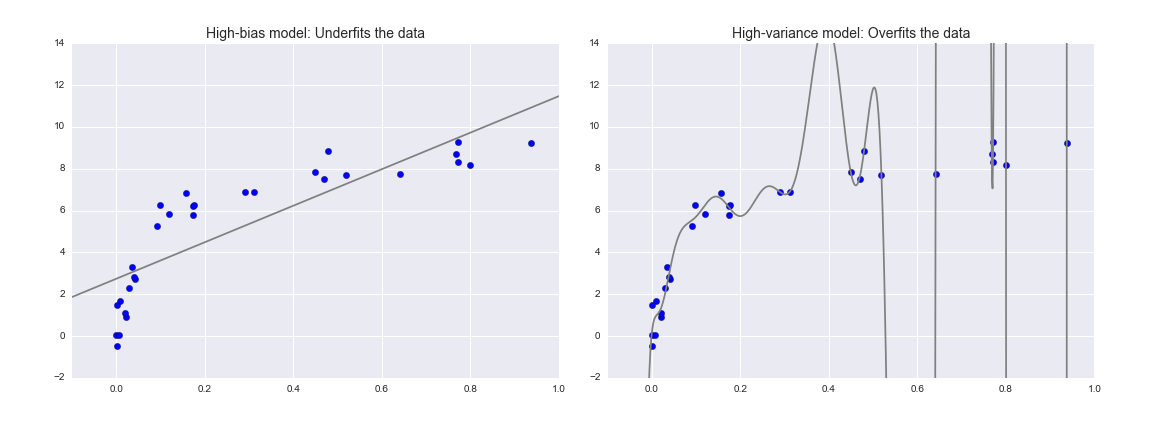
It is clear that neither of these models is a particularly good fit to the data, but they fail in different ways.
The model on the left attempts to find a straight-line fit through the data. Because the data are intrinsically more complicated than a straight line, the straight-line model will never be able to describe this dataset well. Such a model is said to underfit the data; that is, it does not have enough model flexibility to suitably account for all the features in the data. Another way of saying this is that the model has high bias.
The model on the right attempts to fit a high-order polynomial through the data. Here the model fit has enough flexibility to nearly perfectly account for the fine features in the data, but even though it very accurately describes the training data, its precise form seems to be more reflective of the particular noise properties of the data rather than the intrinsic properties of whatever process generated that data. Such a model is said to overfit the data; that is, it has so much model flexibility that the model ends up accounting for random errors as well as the underlying data distribution. Another way of saying this is that the model has high variance.
To look at this in another light, consider what happens if we use these two models to predict the y-value for some new data. In diagrams in Figure 5-25, the red/lighter points indicate data that is omitted from the training set.
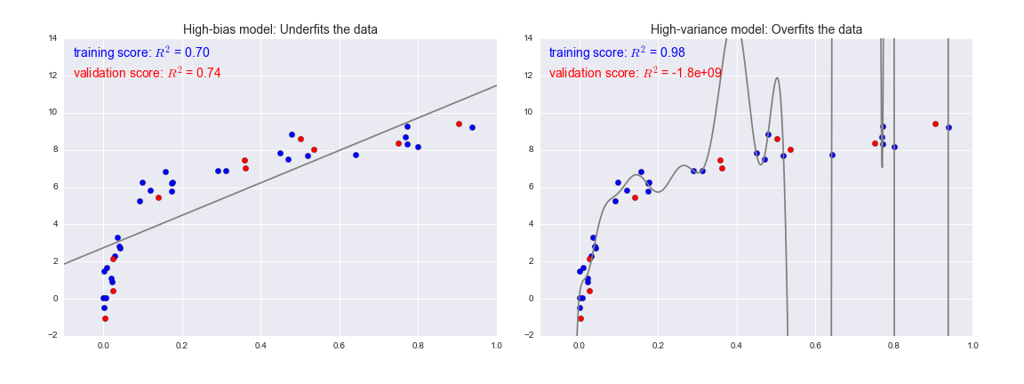
The score here is the  score, or
coefficient
of determination, which measures how well a model performs relative to
a simple mean of the target values.
score, or
coefficient
of determination, which measures how well a model performs relative to
a simple mean of the target values.  indicates a
perfect match,
indicates a
perfect match,  indicates the model does no better
than simply taking the mean of the data, and negative values mean even
worse models. From the scores associated with these two models, we can
make an observation that holds more generally:
indicates the model does no better
than simply taking the mean of the data, and negative values mean even
worse models. From the scores associated with these two models, we can
make an observation that holds more generally:
For high-bias models, the performance of the model on the validation set is similar to the performance on the training set.
For high-variance models, the performance of the model on the validation set is far worse than the performance on the training set.
If we imagine that we have some ability to tune the model complexity, we would expect the training score and validation score to behave as illustrated in Figure 5-26.
The diagram shown in Figure 5-26 is often called a validation curve, and we see the following essential features:
The training score is everywhere higher than the validation score. This is generally the case: the model will be a better fit to data it has seen than to data it has not seen.
For very low model complexity (a high-bias model), the training data is underfit, which means that the model is a poor predictor both for the training data and for any previously unseen data.
For very high model complexity (a high-variance model), the training data is overfit, which means that the model predicts the training data very well, but fails for any previously unseen data.
For some intermediate value, the validation curve has a maximum. This level of complexity indicates a suitable trade-off between bias and variance.
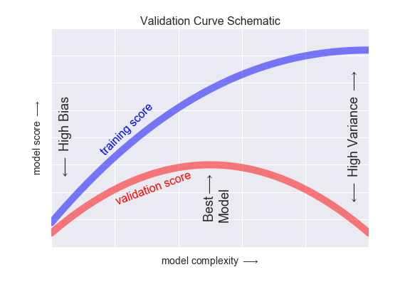
The means of tuning the model complexity varies from model to model; when we discuss individual models in depth in later sections, we will see how each model allows for such tuning.
Let’s look at an example of using cross-validation to compute the
validation curve for a class of models. Here we will use a polynomial regression model: this is a generalized linear model in which the
degree of the polynomial is a tunable parameter. For example, a degree-1
polynomial fits a straight line to the data; for model parameters
 and
and  :
:
A degree-3 polynomial fits a cubic curve to the data; for model
parameters  :
:
We can generalize this to any number of polynomial features. In Scikit-Learn, we can implement this with a simple linear regression combined with the polynomial preprocessor. We will use a pipeline to string these operations together (we will discuss polynomial features and pipelines more fully in “Feature Engineering”):
In[10]:fromsklearn.preprocessingimportPolynomialFeaturesfromsklearn.linear_modelimportLinearRegressionfromsklearn.pipelineimportmake_pipelinedefPolynomialRegression(degree=2,**kwargs):returnmake_pipeline(PolynomialFeatures(degree),LinearRegression(**kwargs))
Now let’s create some data to which we will fit our model:
In[11]:importnumpyasnpdefmake_data(N,err=1.0,rseed=1):# randomly sample the datarng=np.random.RandomState(rseed)X=rng.rand(N,1)**2y=10-1./(X.ravel()+0.1)iferr>0:y+=err*rng.randn(N)returnX,yX,y=make_data(40)
We can now visualize our data, along with polynomial fits of several degrees (Figure 5-27):
In[12]:%matplotlibinlineimportmatplotlib.pyplotaspltimportseaborn;seaborn.set()# plot formattingX_test=np.linspace(-0.1,1.1,500)[:,None]plt.scatter(X.ravel(),y,color='black')axis=plt.axis()fordegreein[1,3,5]:y_test=PolynomialRegression(degree).fit(X,y).predict(X_test)plt.plot(X_test.ravel(),y_test,label='degree={0}'.format(degree))plt.xlim(-0.1,1.0)plt.ylim(-2,12)plt.legend(loc='best');
The knob controlling model complexity in this case is the degree of the polynomial, which can be any non-negative integer. A useful question to answer is this: what degree of polynomial provides a suitable trade-off between bias (underfitting) and variance (overfitting)?
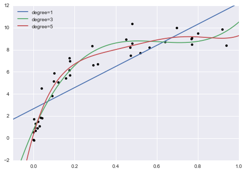
We can make progress in this by visualizing the validation curve for
this particular data and model; we can do this straightforwardly using
the validation_curve convenience routine provided by Scikit-Learn.
Given a model, data, parameter name, and a range to explore, this
function will automatically compute both the training score and
validation score across the range (Figure 5-28):
In[13]:fromsklearn.learning_curveimportvalidation_curvedegree=np.arange(0,21)train_score,val_score=validation_curve(PolynomialRegression(),X,y,'polynomialfeatures__degree',degree,cv=7)plt.plot(degree,np.median(train_score,1),color='blue',label='training score')plt.plot(degree,np.median(val_score,1),color='red',label='validation score')plt.legend(loc='best')plt.ylim(0,1)plt.xlabel('degree')plt.ylabel('score');
This shows precisely the qualitative behavior we expect: the training score is everywhere higher than the validation score; the training score is monotonically improving with increased model complexity; and the validation score reaches a maximum before dropping off as the model becomes overfit.
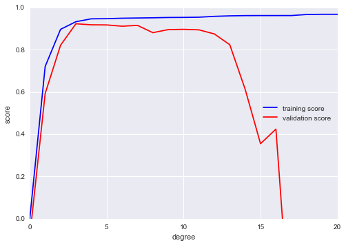
From the validation curve, we can read off that the optimal trade-off between bias and variance is found for a third-order polynomial; we can compute and display this fit over the original data as follows (Figure 5-29):
In[14]:plt.scatter(X.ravel(),y)lim=plt.axis()y_test=PolynomialRegression(3).fit(X,y).predict(X_test)plt.plot(X_test.ravel(),y_test);plt.axis(lim);
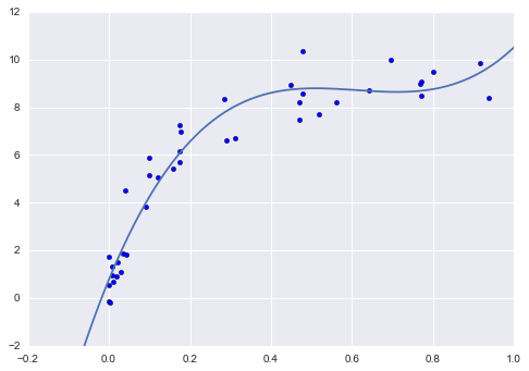
Notice that finding this optimal model did not actually require us to compute the training score, but examining the relationship between the training score and validation score can give us useful insight into the performance of the model.
One important aspect of model complexity is that the optimal model will generally depend on the size of your training data. For example, let’s generate a new dataset with a factor of five more points (Figure 5-30):
In[15]:X2,y2=make_data(200)plt.scatter(X2.ravel(),y2);
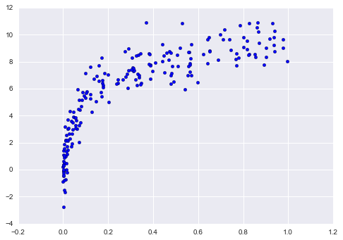
We will duplicate the preceding code to plot the validation curve for this larger dataset; for reference let’s over-plot the previous results as well (Figure 5-31):
In[16]:degree=np.arange(21)train_score2,val_score2=validation_curve(PolynomialRegression(),X2,y2,'polynomialfeatures__degree',degree,cv=7)plt.plot(degree,np.median(train_score2,1),color='blue',label='training score')plt.plot(degree,np.median(val_score2,1),color='red',label='validation score')plt.plot(degree,np.median(train_score,1),color='blue',alpha=0.3,linestyle='dashed')plt.plot(degree,np.median(val_score,1),color='red',alpha=0.3,linestyle='dashed')plt.legend(loc='lower center')plt.ylim(0,1)plt.xlabel('degree')plt.ylabel('score');
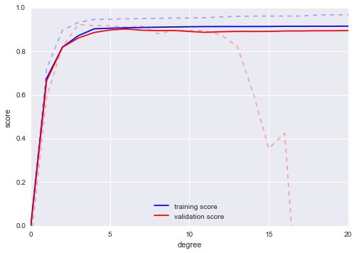
The solid lines show the new results, while the fainter dashed lines show the results of the previous smaller dataset. It is clear from the validation curve that the larger dataset can support a much more complicated model: the peak here is probably around a degree of 6, but even a degree-20 model is not seriously overfitting the data—the validation and training scores remain very close.
Thus we see that the behavior of the validation curve has not one, but two, important inputs: the model complexity and the number of training points. It is often useful to explore the behavior of the model as a function of the number of training points, which we can do by using increasingly larger subsets of the data to fit our model. A plot of the training/validation score with respect to the size of the training set is known as a learning curve.
The general behavior we would expect from a learning curve is this:
A model of a given complexity will overfit a small dataset: this means the training score will be relatively high, while the validation score will be relatively low.
A model of a given complexity will underfit a large dataset: this means that the training score will decrease, but the validation score will increase.
A model will never, except by chance, give a better score to the validation set than the training set: this means the curves should keep getting closer together but never cross.
With these features in mind, we would expect a learning curve to look qualitatively like that shown in Figure 5-32.
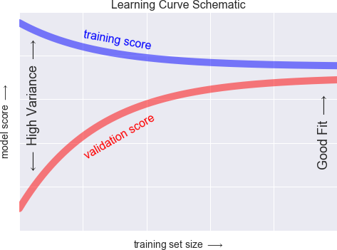
The notable feature of the learning curve is the convergence to a particular score as the number of training samples grows. In particular, once you have enough points that a particular model has converged, adding more training data will not help you! The only way to increase model performance in this case is to use another (often more complex) model.
Scikit-Learn offers a convenient utility for computing such learning curves from your models; here we will compute a learning curve for our original dataset with a second-order polynomial model and a ninth-order polynomial (Figure 5-33):
In[17]:fromsklearn.learning_curveimportlearning_curvefig,ax=plt.subplots(1,2,figsize=(16,6))fig.subplots_adjust(left=0.0625,right=0.95,wspace=0.1)fori,degreeinenumerate([2,9]):N,train_lc,val_lc=learning_curve(PolynomialRegression(degree),X,y,cv=7,train_sizes=np.linspace(0.3,1,25))ax[i].plot(N,np.mean(train_lc,1),color='blue',label='training score')ax[i].plot(N,np.mean(val_lc,1),color='red',label='validation score')ax[i].hlines(np.mean([train_lc[-1],val_lc[-1]]),N[0],N[-1],color='gray',linestyle='dashed')ax[i].set_ylim(0,1)ax[i].set_xlim(N[0],N[-1])ax[i].set_xlabel('training size')ax[i].set_ylabel('score')ax[i].set_title('degree = {0}'.format(degree),size=14)ax[i].legend(loc='best')
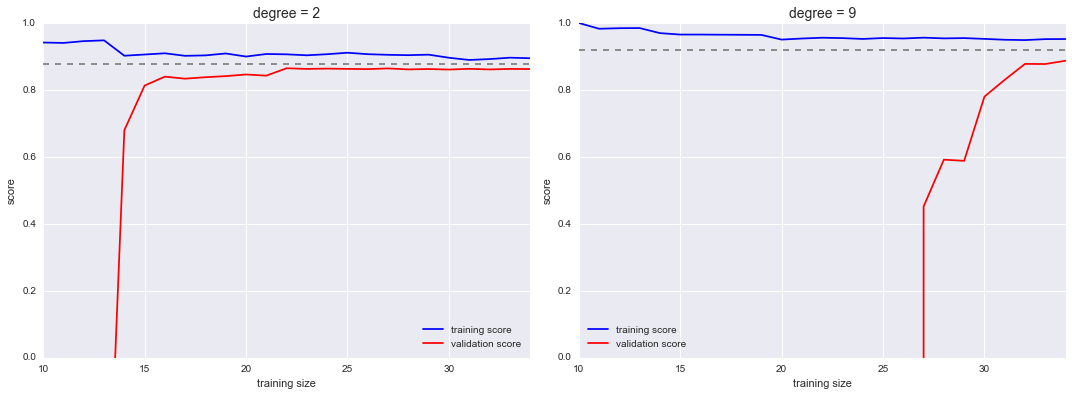
This is a valuable diagnostic, because it gives us a visual depiction of how our model responds to increasing training data. In particular, when your learning curve has already converged (i.e., when the training and validation curves are already close to each other), adding more training data will not significantly improve the fit! This situation is seen in the left panel, with the learning curve for the degree-2 model.
The only way to increase the converged score is to use a different (usually more complicated) model. We see this in the right panel: by moving to a much more complicated model, we increase the score of convergence (indicated by the dashed line), but at the expense of higher model variance (indicated by the difference between the training and validation scores). If we were to add even more data points, the learning curve for the more complicated model would eventually converge.
Plotting a learning curve for your particular choice of model and dataset can help you to make this type of decision about how to move forward in improving your analysis.
The preceding discussion is meant to give you some intuition into the trade-off between bias and variance, and its dependence on model complexity and training set size. In practice, models generally have more than one knob to turn, and thus plots of validation and learning curves change from lines to multidimensional surfaces. In these cases, such visualizations are difficult and we would rather simply find the particular model that maximizes the validation score.
Scikit-Learn provides automated tools to do this in the grid_search
module. Here is an example of using grid search to find the optimal
polynomial model. We will explore a three-dimensional grid of model
features—namely, the polynomial degree, the flag telling us whether to
fit the intercept, and the flag telling us whether to normalize the
problem. We can set this up using Scikit-Learn’s GridSearchCV
meta-estimator:
In[18]:fromsklearn.grid_searchimportGridSearchCVparam_grid={'polynomialfeatures__degree':np.arange(21),'linearregression__fit_intercept':[True,False],'linearregression__normalize':[True,False]}grid=GridSearchCV(PolynomialRegression(),param_grid,cv=7)
Notice that like a normal estimator, this has not yet been applied to
any data. Calling the fit() method will fit the model at each grid
point, keeping track of the scores along the way:
In[19]:grid.fit(X,y);
Now that this is fit, we can ask for the best parameters as follows:
In[20]:grid.best_params_
Out[20]: {'linearregression__fit_intercept': False,
'linearregression__normalize': True,
'polynomialfeatures__degree': 4}
Finally, if we wish, we can use the best model and show the fit to our data using code from before (Figure 5-34):
In[21]:model=grid.best_estimator_plt.scatter(X.ravel(),y)lim=plt.axis()y_test=model.fit(X,y).predict(X_test)plt.plot(X_test.ravel(),y_test,hold=True);plt.axis(lim);
The grid search provides many more options, including the ability to specify a custom scoring function, to parallelize the computations, to do randomized searches, and more. For information, see the examples in “In-Depth: Kernel Density Estimation” and “Application: A Face Detection Pipeline”, or refer to Scikit-Learn’s grid search documentation.
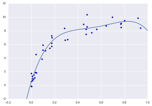
In this section, we have begun to explore the concept of model validation and hyperparameter optimization, focusing on intuitive aspects of the bias–variance trade-off and how it comes into play when fitting models to data. In particular, we found that the use of a validation set or cross-validation approach is vital when tuning parameters in order to avoid overfitting for more complex/flexible models.
In later sections, we will discuss the details of particularly useful models, and throughout will talk about what tuning is available for these models and how these free parameters affect model complexity. Keep the lessons of this section in mind as you read on and learn about these machine learning approaches!
The previous sections outline the fundamental ideas of machine learning,
but all of the examples assume that you have numerical data in a tidy,
[n_samples, n_features] format. In the real world, data rarely comes
in such a form. With this in mind, one of the more important steps in
using machine learning in practice is feature engineering—that is,
taking whatever information you have about your problem and turning it
into numbers that you can use to build your feature matrix.
In this section, we will cover a few common examples of feature engineering tasks: features for representing categorical data, features for representing text, and features for representing images. Additionally, we will discuss derived features for increasing model complexity and imputation of missing data. Often this process is known as vectorization, as it involves converting arbitrary data into well-behaved vectors.
One common type of non-numerical data is categorical data. For example, imagine you are exploring some data on housing prices, and along with numerical features like “price” and “rooms,” you also have “neighborhood” information. For example, your data might look something like this:
In[1]:data=[{'price':850000,'rooms':4,'neighborhood':'Queen Anne'},{'price':700000,'rooms':3,'neighborhood':'Fremont'},{'price':650000,'rooms':3,'neighborhood':'Wallingford'},{'price':600000,'rooms':2,'neighborhood':'Fremont'}]
You might be tempted to encode this data with a straightforward numerical mapping:
In[2]:{'Queen Anne':1,'Fremont':2,'Wallingford':3};
It turns out that this is not generally a useful approach in Scikit-Learn: the package’s models make the fundamental assumption that numerical features reflect algebraic quantities. Thus such a mapping would imply, for example, that Queen Anne < Fremont < Wallingford, or even that Wallingford - Queen Anne = Fremont, which (niche demographic jokes aside) does not make much sense.
In this case, one proven technique is to use one-hot encoding, which
effectively creates extra columns indicating the presence or absence of
a category with a value of 1 or 0, respectively. When your data comes as a
list of dictionaries, Scikit-Learn’s DictVectorizer will do this for
you:
In[3]:fromsklearn.feature_extractionimportDictVectorizervec=DictVectorizer(sparse=False,dtype=int)vec.fit_transform(data)
Out[3]: array([[ 0, 1, 0, 850000, 4],
[ 1, 0, 0, 700000, 3],
[ 0, 0, 1, 650000, 3],
[ 1, 0, 0, 600000, 2]], dtype=int64)
Notice that the neighborhood column has been expanded into three separate columns, representing the three neighborhood labels, and that each row has a 1 in the column associated with its neighborhood. With these categorical features thus encoded, you can proceed as normal with fitting a Scikit-Learn model.
To see the meaning of each column, you can inspect the feature names:
In[4]:vec.get_feature_names()
Out[4]: ['neighborhood=Fremont',
'neighborhood=Queen Anne',
'neighborhood=Wallingford',
'price',
'rooms']
There is one clear disadvantage of this approach: if your category has many possible values, this can greatly increase the size of your dataset. However, because the encoded data contains mostly zeros, a sparse output can be a very efficient solution:
In[5]:vec=DictVectorizer(sparse=True,dtype=int)vec.fit_transform(data)
Out[5]: <4x5 sparse matrix of type '<class 'numpy.int64'>'
with 12 stored elements in Compressed Sparse Row format>
Many (though not yet all) of the Scikit-Learn estimators accept such
sparse inputs when fitting and evaluating models. sklearn.preprocessing.OneHotEncoder and
sklearn.feature_extraction.FeatureHasher are two additional tools that Scikit-Learn includes to support this type of encoding.
Another common need in feature engineering is to convert text to a set of representative numerical values. For example, most automatic mining of social media data relies on some form of encoding the text as numbers. One of the simplest methods of encoding data is by word counts: you take each snippet of text, count the occurrences of each word within it, and put the results in a table.
For example, consider the following set of three phrases:
In[6]:sample=['problem of evil','evil queen','horizon problem']
For a vectorization of this data based on word count, we could construct
a column representing the word “problem,” the word “evil,” the word
“horizon,” and so on. While doing this by hand would be possible, we can avoid the tedium by using Scikit-Learn’s CountVectorizer:
In[7]:fromsklearn.feature_extraction.textimportCountVectorizervec=CountVectorizer()X=vec.fit_transform(sample)X
Out[7]: <3x5 sparse matrix of type '<class 'numpy.int64'>'
with 7 stored elements in Compressed Sparse Row format>
The result is a sparse matrix recording the number of times each word
appears; it is easier to inspect if we convert this to a DataFrame with
labeled columns:
In[8]:importpandasaspdpd.DataFrame(X.toarray(),columns=vec.get_feature_names())
Out[8]: evil horizon of problem queen
0 1 0 1 1 0
1 1 0 0 0 1
2 0 1 0 1 0
There are some issues with this approach, however: the raw word counts lead to features that put too much weight on words that appear very frequently, and this can be suboptimal in some classification algorithms. One approach to fix this is known as term frequency–inverse document frequency (TF–IDF), which weights the word counts by a measure of how often they appear in the documents. The syntax for computing these features is similar to the previous example:
In[9]:fromsklearn.feature_extraction.textimportTfidfVectorizervec=TfidfVectorizer()X=vec.fit_transform(sample)pd.DataFrame(X.toarray(),columns=vec.get_feature_names())
Out[9]: evil horizon of problem queen
0 0.517856 0.000000 0.680919 0.517856 0.000000
1 0.605349 0.000000 0.000000 0.000000 0.795961
2 0.000000 0.795961 0.000000 0.605349 0.000000
For an example of using TF–IDF in a classification problem, see “In Depth: Naive Bayes Classification”.
Another common need is to suitably encode images for machine learning analysis. The simplest approach is what we used for the digits data in “Introducing Scikit-Learn”: simply using the pixel values themselves. But depending on the application, such approaches may not be optimal.
A comprehensive summary of feature extraction techniques for images is well beyond the scope of this section, but you can find excellent implementations of many of the standard approaches in the Scikit-Image project. For one example of using Scikit-Learn and Scikit-Image together, see “Application: A Face Detection Pipeline”.
Another useful type of feature is one that is mathematically derived from some input features. We saw an example of this in “Hyperparameters and Model Validation” when we constructed polynomial features from our input data. We saw that we could convert a linear regression into a polynomial regression not by changing the model, but by transforming the input! This is sometimes known as basis function regression, and is explored further in “In Depth: Linear Regression”.
For example, this data clearly cannot be well described by a straight line (Figure 5-35):
In[10]:%matplotlibinlineimportnumpyasnpimportmatplotlib.pyplotaspltx=np.array([1,2,3,4,5])y=np.array([4,2,1,3,7])plt.scatter(x,y);
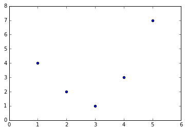
Still, we can fit a line to the data using LinearRegression and get
the optimal result (Figure 5-36):
In[11]:fromsklearn.linear_modelimportLinearRegressionX=x[:,np.newaxis]model=LinearRegression().fit(X,y)yfit=model.predict(X)plt.scatter(x,y)plt.plot(x,yfit);
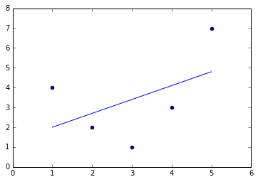
It’s clear that we need a more sophisticated model to describe the
relationship between  and
and  . We can do this by transforming the data, adding extra columns of features to drive
more flexibility in the model. For example, we can add polynomial
features to the data this way:
. We can do this by transforming the data, adding extra columns of features to drive
more flexibility in the model. For example, we can add polynomial
features to the data this way:
In[12]:fromsklearn.preprocessingimportPolynomialFeaturespoly=PolynomialFeatures(degree=3,include_bias=False)X2=poly.fit_transform(X)(X2)
[[ 1. 1. 1.] [ 2. 4. 8.] [ 3. 9. 27.] [ 4. 16. 64.] [ 5. 25. 125.]]
The derived feature matrix has one column representing  ,
and a second column representing
,
and a second column representing  , and a third column
representing
, and a third column
representing  . Computing a linear regression on this
expanded input gives a much closer fit to our data (Figure 5-37):
. Computing a linear regression on this
expanded input gives a much closer fit to our data (Figure 5-37):
In[13]:model=LinearRegression().fit(X2,y)yfit=model.predict(X2)plt.scatter(x,y)plt.plot(x,yfit);
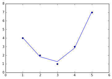
This idea of improving a model not by changing the model, but by transforming the inputs, is fundamental to many of the more powerful machine learning methods. We explore this idea further in “In Depth: Linear Regression” in the context of basis function regression. More generally, this is one motivational path to the powerful set of techniques known as kernel methods, which we will explore in “In-Depth: Support Vector Machines”.
Another common need in feature engineering is handling missing data.
We discussed the handling of missing data in DataFrames in
“Handling Missing Data”, and saw that
often the NaN value is used to mark missing values. For example, we
might have a dataset that looks like this:
In[14]:fromnumpyimportnanX=np.array([[nan,0,3],[3,7,9],[3,5,2],[4,nan,6],[8,8,1]])y=np.array([14,16,-1,8,-5])
When applying a typical machine learning model to such data, we will need to first replace such missing data with some appropriate fill value. This is known as imputation of missing values, and strategies range from simple (e.g., replacing missing values with the mean of the column) to sophisticated (e.g., using matrix completion or a robust model to handle such data).
The sophisticated approaches tend to be very application-specific, and
we won’t dive into them here. For a baseline imputation approach, using
the mean, median, or most frequent value, Scikit-Learn provides the
Imputer class:
In[15]:fromsklearn.preprocessingimportImputerimp=Imputer(strategy='mean')X2=imp.fit_transform(X)X2
Out[15]: array([[ 4.5, 0. , 3. ],
[ 3. , 7. , 9. ],
[ 3. , 5. , 2. ],
[ 4. , 5. , 6. ],
[ 8. , 8. , 1. ]])
We see that in the resulting data, the two missing values have been
replaced with the mean of the remaining values in the column. This
imputed data can then be fed directly into, for example, a LinearRegression
estimator:
In[16]:model=LinearRegression().fit(X2,y)model.predict(X2)
Out[16]: array([ 13.14869292, 14.3784627 , -1.15539732, 10.96606197, -5.33782027])
With any of the preceding examples, it can quickly become tedious to do the transformations by hand, especially if you wish to string together multiple steps. For example, we might want a processing pipeline that looks something like this:
Impute missing values using the mean
Transform features to quadratic
Fit a linear regression
To streamline this type of processing pipeline, Scikit-Learn provides a pipeline object, which can be used as follows:
In[17]:fromsklearn.pipelineimportmake_pipelinemodel=make_pipeline(Imputer(strategy='mean'),PolynomialFeatures(degree=2),LinearRegression())
This pipeline looks and acts like a standard Scikit-Learn object, and will apply all the specified steps to any input data.
In[18]:model.fit(X,y)# X with missing values, from above(y)(model.predict(X))
[14 16 -1 8 -5] [ 14. 16. -1. 8. -5.]
All the steps of the model are applied automatically. Notice that for the simplicity of this demonstration, we’ve applied the model to the data it was trained on; this is why it was able to perfectly predict the result (refer back to “Hyperparameters and Model Validation” for further discussion of this).
For some examples of Scikit-Learn pipelines in action, see the following section on naive Bayes classification as well as “In Depth: Linear Regression” and “In-Depth: Support Vector Machines”.
The previous four sections have given a general overview of the concepts of machine learning. In this section and the ones that follow, we will be taking a closer look at several specific algorithms for supervised and unsupervised learning, starting here with naive Bayes classification.
Naive Bayes models are a group of extremely fast and simple classification algorithms that are often suitable for very high-dimensional datasets. Because they are so fast and have so few tunable parameters, they end up being very useful as a quick-and-dirty baseline for a classification problem. This section will focus on an intuitive explanation of how naive Bayes classifiers work, followed by a couple examples of them in action on some datasets.
Naive Bayes classifiers are built on Bayesian classification methods.
These rely on Bayes’s theorem, which is an equation describing the
relationship of conditional probabilities of statistical quantities. In
Bayesian classification, we’re interested in finding the probability of
a label given some observed features, which we can write as
 . Bayes’s theorem tells us how to
express this in terms of quantities we can compute more directly:
. Bayes’s theorem tells us how to
express this in terms of quantities we can compute more directly:
If we are trying to decide between two labels—let’s call them
 and
and  —then one way to make this
decision is to compute the ratio of the posterior probabilities for each
label:
—then one way to make this
decision is to compute the ratio of the posterior probabilities for each
label:
All we need now is some model by which we can compute
 for each label. Such a model is
called a generative model because it specifies the hypothetical random
process that generates the data. Specifying this generative model for
each label is the main piece of the training of such a Bayesian
classifier. The general version of such a training step is a very
difficult task, but we can make it simpler through the use of some
simplifying assumptions about the form of this model.
for each label. Such a model is
called a generative model because it specifies the hypothetical random
process that generates the data. Specifying this generative model for
each label is the main piece of the training of such a Bayesian
classifier. The general version of such a training step is a very
difficult task, but we can make it simpler through the use of some
simplifying assumptions about the form of this model.
This is where the “naive” in “naive Bayes” comes in: if we make very naive assumptions about the generative model for each label, we can find a rough approximation of the generative model for each class, and then proceed with the Bayesian classification. Different types of naive Bayes classifiers rest on different naive assumptions about the data, and we will examine a few of these in the following sections. We begin with the standard imports:
In[1]:%matplotlibinlineimportnumpyasnpimportmatplotlib.pyplotaspltimportseabornassns;sns.set()
Perhaps the easiest naive Bayes classifier to understand is Gaussian naive Bayes. In this classifier, the assumption is that data from each label is drawn from a simple Gaussian distribution. Imagine that you have the following data (Figure 5-38):
In[2]:fromsklearn.datasetsimportmake_blobsX,y=make_blobs(100,2,centers=2,random_state=2,cluster_std=1.5)plt.scatter(X[:,0],X[:,1],c=y,s=50,cmap='RdBu');
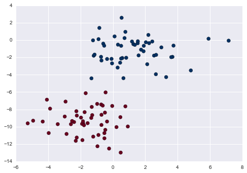
One extremely fast way to create a simple model is to assume that the data is described by a Gaussian distribution with no covariance between dimensions. We can fit this model by simply finding the mean and standard deviation of the points within each label, which is all you need to define such a distribution. The result of this naive Gaussian assumption is shown in Figure 5-39.
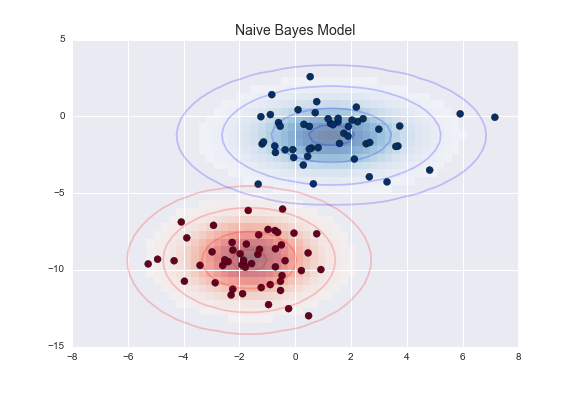
The ellipses here represent the Gaussian generative model for each
label, with larger probability toward the center of the ellipses. With
this generative model in place for each class, we have a simple recipe
to compute the likelihood 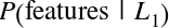 for any
data point, and thus we can quickly compute the posterior ratio and
determine which label is the most probable for a given point.
for any
data point, and thus we can quickly compute the posterior ratio and
determine which label is the most probable for a given point.
This procedure is implemented in Scikit-Learn’s sklearn.naive_bayes.GaussianNB estimator:
In[3]:fromsklearn.naive_bayesimportGaussianNBmodel=GaussianNB()model.fit(X,y);
Now let’s generate some new data and predict the label:
In[4]:rng=np.random.RandomState(0)Xnew=[-6,-14]+[14,18]*rng.rand(2000,2)ynew=model.predict(Xnew)
Now we can plot this new data to get an idea of where the decision boundary is (Figure 5-40):
In[5]:plt.scatter(X[:,0],X[:,1],c=y,s=50,cmap='RdBu')lim=plt.axis()plt.scatter(Xnew[:,0],Xnew[:,1],c=ynew,s=20,cmap='RdBu',alpha=0.1)plt.axis(lim);
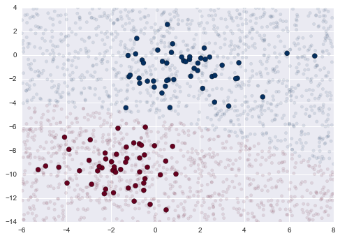
We see a slightly curved boundary in the classifications—in general, the boundary in Gaussian naive Bayes is quadratic.
A nice piece of this Bayesian formalism is that it naturally allows for
probabilistic classification, which we can compute using the
predict_proba method:
In[6]:yprob=model.predict_proba(Xnew)yprob[-8:].round(2)
Out[6]: array([[ 0.89, 0.11],
[ 1. , 0. ],
[ 1. , 0. ],
[ 1. , 0. ],
[ 1. , 0. ],
[ 1. , 0. ],
[ 0. , 1. ],
[ 0.15, 0.85]])
The columns give the posterior probabilities of the first and second label, respectively. If you are looking for estimates of uncertainty in your classification, Bayesian approaches like this can be a useful approach.
Of course, the final classification will only be as good as the model assumptions that lead to it, which is why Gaussian naive Bayes often does not produce very good results. Still, in many cases—especially as the number of features becomes large—this assumption is not detrimental enough to prevent Gaussian naive Bayes from being a useful method.
The Gaussian assumption just described is by no means the only simple assumption that could be used to specify the generative distribution for each label. Another useful example is multinomial naive Bayes, where the features are assumed to be generated from a simple multinomial distribution. The multinomial distribution describes the probability of observing counts among a number of categories, and thus multinomial naive Bayes is most appropriate for features that represent counts or count rates.
The idea is precisely the same as before, except that instead of modeling the data distribution with the best-fit Gaussian, we model the data distribution with a best-fit multinomial distribution.
One place where multinomial naive Bayes is often used is in text classification, where the features are related to word counts or frequencies within the documents to be classified. We discussed the extraction of such features from text in “Feature Engineering”; here we will use the sparse word count features from the 20 Newsgroups corpus to show how we might classify these short documents into categories.
Let’s download the data and take a look at the target names:
In[7]:fromsklearn.datasetsimportfetch_20newsgroupsdata=fetch_20newsgroups()data.target_names
Out[7]: ['alt.atheism',
'comp.graphics',
'comp.os.ms-windows.misc',
'comp.sys.ibm.pc.hardware',
'comp.sys.mac.hardware',
'comp.windows.x',
'misc.forsale',
'rec.autos',
'rec.motorcycles',
'rec.sport.baseball',
'rec.sport.hockey',
'sci.crypt',
'sci.electronics',
'sci.med',
'sci.space',
'soc.religion.christian',
'talk.politics.guns',
'talk.politics.mideast',
'talk.politics.misc',
'talk.religion.misc']
For simplicity, we will select just a few of these categories, and download the training and testing set:
In[8]:categories=['talk.religion.misc','soc.religion.christian','sci.space','comp.graphics']train=fetch_20newsgroups(subset='train',categories=categories)test=fetch_20newsgroups(subset='test',categories=categories)
Here is a representative entry from the data:
In[9]:(train.data[5])
From: dmcgee@uluhe.soest.hawaii.edu (Don McGee) Subject: Federal Hearing Originator: dmcgee@uluhe Organization: School of Ocean and Earth Science and Technology Distribution: usa Lines: 10 Fact or rumor....? Madalyn Murray O'Hare an atheist who eliminated the use of the bible reading and prayer in public schools 15 years ago is now going to appear before the FCC with a petition to stop the reading of the Gospel on the airways of America. And she is also campaigning to remove Christmas programs, songs, etc from the public schools. If it is true then mail to Federal Communications Commission 1919 H Street Washington DC 20054 expressing your opposition to her request. Reference Petition number 2493.
In order to use this data for machine learning, we need to be able to convert the content of each string into a vector of numbers. For this we will use the TF–IDF vectorizer (discussed in “Feature Engineering”), and create a pipeline that attaches it to a multinomial naive Bayes classifier:
In[10]:fromsklearn.feature_extraction.textimportTfidfVectorizerfromsklearn.naive_bayesimportMultinomialNBfromsklearn.pipelineimportmake_pipelinemodel=make_pipeline(TfidfVectorizer(),MultinomialNB())
With this pipeline, we can apply the model to the training data, and predict labels for the test data:
In[11]:model.fit(train.data,train.target)labels=model.predict(test.data)
Now that we have predicted the labels for the test data, we can evaluate them to learn about the performance of the estimator. For example, here is the confusion matrix between the true and predicted labels for the test data (Figure 5-41):
In[12]:fromsklearn.metricsimportconfusion_matrixmat=confusion_matrix(test.target,labels)sns.heatmap(mat.T,square=True,annot=True,fmt='d',cbar=False,xticklabels=train.target_names,yticklabels=train.target_names)plt.xlabel('true label')plt.ylabel('predicted label');
Evidently, even this very simple classifier can successfully separate space talk from computer talk, but it gets confused between talk about religion and talk about Christianity. This is perhaps an expected area of confusion!
The very cool thing here is that we now have the tools to determine the
category for any string, using the predict() method of this
pipeline. Here’s a quick utility function that will return the
prediction for a single string:
In[13]:defpredict_category(s,train=train,model=model):pred=model.predict([s])returntrain.target_names[pred[0]]
Let’s try it out:
In[14]:predict_category('sending a payload to the ISS')
Out[14]: 'sci.space'
In[15]:predict_category('discussing islam vs atheism')
Out[15]: 'soc.religion.christian'
In[16]:predict_category('determining the screen resolution')
Out[16]: 'comp.graphics'
Remember that this is nothing more sophisticated than a simple probability model for the (weighted) frequency of each word in the string; nevertheless, the result is striking. Even a very naive algorithm, when used carefully and trained on a large set of high-dimensional data, can be surprisingly effective.
Because naive Bayesian classifiers make such stringent assumptions about data, they will generally not perform as well as a more complicated model. That said, they have several advantages:
They are extremely fast for both training and prediction
They provide straightforward probabilistic prediction
They are often very easily interpretable
They have very few (if any) tunable parameters
These advantages mean a naive Bayesian classifier is often a good choice as an initial baseline classification. If it performs suitably, then congratulations: you have a very fast, very interpretable classifier for your problem. If it does not perform well, then you can begin exploring more sophisticated models, with some baseline knowledge of how well they should perform.
Naive Bayes classifiers tend to perform especially well in one of the following situations:
When the naive assumptions actually match the data (very rare in practice)
For very well-separated categories, when model complexity is less important
For very high-dimensional data, when model complexity is less important
The last two points seem distinct, but they actually are related: as the dimension of a dataset grows, it is much less likely for any two points to be found close together (after all, they must be close in every single dimension to be close overall). This means that clusters in high dimensions tend to be more separated, on average, than clusters in low dimensions, assuming the new dimensions actually add information. For this reason, simplistic classifiers like naive Bayes tend to work as well or better than more complicated classifiers as the dimensionality grows: once you have enough data, even a simple model can be very powerful.
Just as naive Bayes (discussed earlier in “In Depth: Naive Bayes Classification”) is a good starting point for classification tasks, linear regression models are a good starting point for regression tasks. Such models are popular because they can be fit very quickly, and are very interpretable. You are probably familiar with the simplest form of a linear regression model (i.e., fitting a straight line to data), but such models can be extended to model more complicated data behavior.
In this section we will start with a quick intuitive walk-through of the mathematics behind this well-known problem, before moving on to see how linear models can be generalized to account for more complicated patterns in data. We begin with the standard imports:
In[1]:%matplotlibinlineimportmatplotlib.pyplotaspltimportseabornassns;sns.set()importnumpyasnp
We will start with the most familiar linear regression, a straight-line
fit to data. A straight-line fit is a model of the form y = ax + b
where  is commonly known as the slope, and
 is commonly known as the intercept.
Consider the following data, which is scattered about a line with a slope of 2 and an intercept of –5 (Figure 5-42):
In[2]:rng=np.random.RandomState(1)x=10*rng.rand(50)y=2*x-5+rng.randn(50)plt.scatter(x,y);
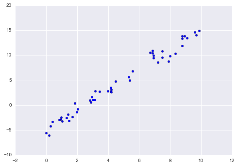
We can use Scikit-Learn’s LinearRegression estimator to fit this data
and construct the best-fit line (Figure 5-43):
In[3]:fromsklearn.linear_modelimportLinearRegressionmodel=LinearRegression(fit_intercept=True)model.fit(x[:,np.newaxis],y)xfit=np.linspace(0,10,1000)yfit=model.predict(xfit[:,np.newaxis])plt.scatter(x,y)plt.plot(xfit,yfit);
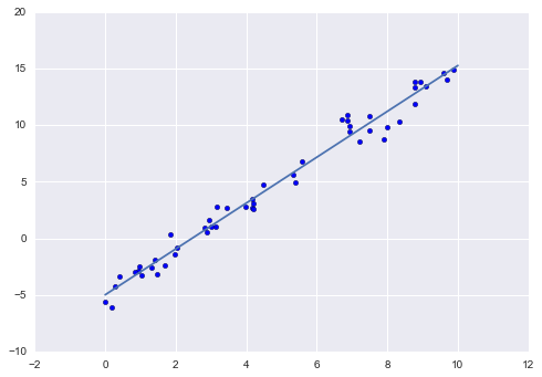
The slope and intercept of the data are contained in the model’s fit
parameters, which in Scikit-Learn are always marked by a trailing
underscore. Here the relevant parameters are coef_ and intercept_:
In[4]:("Model slope: ",model.coef_[0])("Model intercept:",model.intercept_)
Model slope: 2.02720881036 Model intercept: -4.99857708555
We see that the results are very close to the inputs, as we might hope.
The LinearRegression estimator is much more capable than this,
however—in addition to simple straight-line fits, it can also handle
multidimensional linear models of the form:

where there are multiple  values. Geometrically, this
is akin to fitting a plane to points in three dimensions, or fitting a
hyper-plane to points in higher dimensions.
values. Geometrically, this
is akin to fitting a plane to points in three dimensions, or fitting a
hyper-plane to points in higher dimensions.
The multidimensional nature of such regressions makes them more difficult to visualize, but we can see one of these fits in action by building some example data, using NumPy’s matrix multiplication operator:
In[5]:rng=np.random.RandomState(1)X=10*rng.rand(100,3)y=0.5+np.dot(X,[1.5,-2.,1.])model.fit(X,y)(model.intercept_)(model.coef_)
0.5 [ 1.5 -2. 1. ]
Here the  data is constructed from three random
 values, and the linear regression recovers the
coefficients used to construct the data.
values, and the linear regression recovers the
coefficients used to construct the data.
In this way, we can use the single LinearRegression estimator to fit
lines, planes, or hyperplanes to our data. It still appears that this
approach would be limited to strictly linear relationships between
variables, but it turns out we can relax this as well.
One trick you can use to adapt linear regression to nonlinear
relationships between variables is to transform the data according to
basis functions. We have seen one version of this before, in the
PolynomialRegression pipeline used in
“Hyperparameters and Model Validation” and “Feature Engineering”. The idea is to take our multidimensional linear model:

and build the  and so on from our
single-dimensional input
and so on from our
single-dimensional input  . That is, we let
 , where
  is some function
that transforms our data.
is some function
that transforms our data.
For example, if  , our model becomes a
polynomial regression:
, our model becomes a
polynomial regression:

Notice that this is still a linear model—the linearity refers to
the fact that the coefficients  never multiply or
divide each other. What we have effectively done is taken our
one-dimensional
never multiply or
divide each other. What we have effectively done is taken our
one-dimensional  values and projected them into a higher
dimension, so that a linear fit can fit more complicated relationships
between
values and projected them into a higher
dimension, so that a linear fit can fit more complicated relationships
between  and
and  .
.
This polynomial projection is useful enough that it is built into
Scikit-Learn, using the PolynomialFeatures transformer:
In[6]:fromsklearn.preprocessingimportPolynomialFeaturesx=np.array([2,3,4])poly=PolynomialFeatures(3,include_bias=False)poly.fit_transform(x[:,None])
Out[6]: array([[ 2., 4., 8.],
[ 3., 9., 27.],
[ 4., 16., 64.]])
We see here that the transformer has converted our one-dimensional array into a three-dimensional array by taking the exponent of each value. This new, higher-dimensional data representation can then be plugged into a linear regression.
As we saw in “Feature Engineering”, the cleanest way to accomplish this is to use a pipeline. Let’s make a 7th-degree polynomial model in this way:
In[7]:fromsklearn.pipelineimportmake_pipelinepoly_model=make_pipeline(PolynomialFeatures(7),LinearRegression())
With this transform in place, we can use the linear model to fit much
more complicated relationships between  and
and
 . For example, here is a sine wave with noise (Figure 5-44):
In[8]:rng=np.random.RandomState(1)x=10*rng.rand(50)y=np.sin(x)+0.1*rng.randn(50)poly_model.fit(x[:,np.newaxis],y)yfit=poly_model.predict(xfit[:,np.newaxis])plt.scatter(x,y)plt.plot(xfit,yfit);
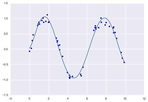
Our linear model, through the use of 7th-order polynomial basis functions, can provide an excellent fit to this nonlinear data!
Of course, other basis functions are possible. For example, one useful pattern is to fit a model that is not a sum of polynomial bases, but a sum of Gaussian bases. The result might look something like Figure 5-45.
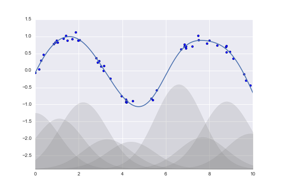
The shaded regions in the plot shown in Figure 5-45 are the scaled basis functions, and when added together they reproduce the smooth curve through the data. These Gaussian basis functions are not built into Scikit-Learn, but we can write a custom transformer that will create them, as shown here and illustrated in Figure 5-46 (Scikit-Learn transformers are implemented as Python classes; reading Scikit-Learn’s source is a good way to see how they can be created):
In[9]:fromsklearn.baseimportBaseEstimator,TransformerMixinclassGaussianFeatures(BaseEstimator,TransformerMixin):"""Uniformly spaced Gaussian features for one-dimensional input"""def__init__(self,N,width_factor=2.0):self.N=Nself.width_factor=width_factor@staticmethoddef_gauss_basis(x,y,width,axis=None):arg=(x-y)/widthreturnnp.exp(-0.5*np.sum(arg**2,axis))deffit(self,X,y=None):# create N centers spread along the data rangeself.centers_=np.linspace(X.min(),X.max(),self.N)self.width_=self.width_factor*(self.centers_[1]-self.centers_[0])returnselfdeftransform(self,X):returnself._gauss_basis(X[:,:,np.newaxis],self.centers_,self.width_,axis=1)gauss_model=make_pipeline(GaussianFeatures(20),LinearRegression())gauss_model.fit(x[:,np.newaxis],y)yfit=gauss_model.predict(xfit[:,np.newaxis])plt.scatter(x,y)plt.plot(xfit,yfit)plt.xlim(0,10);
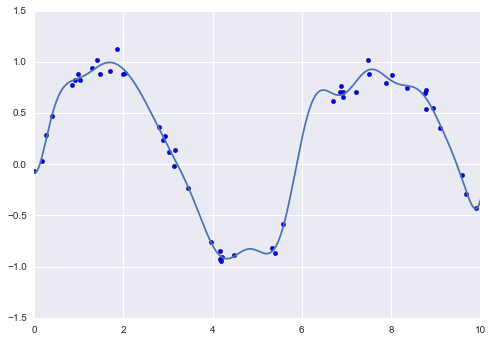
We put this example here just to make clear that there is nothing magic about polynomial basis functions: if you have some sort of intuition into the generating process of your data that makes you think one basis or another might be appropriate, you can use them as well.
The introduction of basis functions into our linear regression makes the model much more flexible, but it also can very quickly lead to overfitting (refer back to “Hyperparameters and Model Validation” for a discussion of this). For example, if we choose too many Gaussian basis functions, we end up with results that don’t look so good (Figure 5-47):
In[10]:model=make_pipeline(GaussianFeatures(30),LinearRegression())model.fit(x[:,np.newaxis],y)plt.scatter(x,y)plt.plot(xfit,model.predict(xfit[:,np.newaxis]))plt.xlim(0,10)plt.ylim(-1.5,1.5);
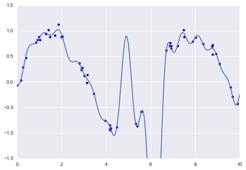
With the data projected to the 30-dimensional basis, the model has far too much flexibility and goes to extreme values between locations where it is constrained by data. We can see the reason for this if we plot the coefficients of the Gaussian bases with respect to their locations (Figure 5-48):
In[11]:defbasis_plot(model,title=None):fig,ax=plt.subplots(2,sharex=True)model.fit(x[:,np.newaxis],y)ax[0].scatter(x,y)ax[0].plot(xfit,model.predict(xfit[:,np.newaxis]))ax[0].set(xlabel='x',ylabel='y',ylim=(-1.5,1.5))iftitle:ax[0].set_title(title)ax[1].plot(model.steps[0][1].centers_,model.steps[1][1].coef_)ax[1].set(xlabel='basis location',ylabel='coefficient',xlim=(0,10))model=make_pipeline(GaussianFeatures(30),LinearRegression())basis_plot(model)
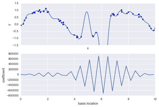
The lower panel in Figure 5-48 shows the amplitude of the basis function at each location. This is typical overfitting behavior when basis functions overlap: the coefficients of adjacent basis functions blow up and cancel each other out. We know that such behavior is problematic, and it would be nice if we could limit such spikes explicitly in the model by penalizing large values of the model parameters. Such a penalty is known as regularization, and comes in several forms.
 regularization)
Perhaps the most common form of regularization is known as ridge
regression or  regularization, sometimes also called
Tikhonov regularization. This proceeds by penalizing the sum of
squares (2-norms) of the model coefficients; in this case, the penalty
on the model fit would be:
regularization, sometimes also called
Tikhonov regularization. This proceeds by penalizing the sum of
squares (2-norms) of the model coefficients; in this case, the penalty
on the model fit would be:
where  is a free parameter that controls the
strength of the penalty. This type of penalized model is built into
Scikit-Learn with the
is a free parameter that controls the
strength of the penalty. This type of penalized model is built into
Scikit-Learn with the Ridge estimator (Figure 5-49):
In[12]:fromsklearn.linear_modelimportRidgemodel=make_pipeline(GaussianFeatures(30),Ridge(alpha=0.1))basis_plot(model,title='Ridge Regression')
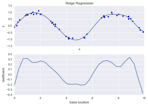
 ) regularization applied to the overly complex model (compare to Figure 5-48)
The  parameter is essentially a knob controlling the
complexity of the resulting model. In the limit
parameter is essentially a knob controlling the
complexity of the resulting model. In the limit
 , we recover the standard linear regression
result; in the limit
, we recover the standard linear regression
result; in the limit  , all model responses
will be suppressed. One advantage of ridge regression in particular is
that it can be computed very efficiently—at hardly more computational
cost than the original linear regression model.
, all model responses
will be suppressed. One advantage of ridge regression in particular is
that it can be computed very efficiently—at hardly more computational
cost than the original linear regression model.
 )
)Another very common type of regularization is known as lasso, and involves penalizing the sum of absolute values (1-norms) of regression coefficients:
Though this is conceptually very similar to ridge regression, the results can differ surprisingly: for example, due to geometric reasons lasso regression tends to favor sparse models where possible; that is, it preferentially sets model coefficients to exactly zero.
We can see this behavior in duplicating the plot shown in Figure 5-49, but using L1-normalized coefficients (Figure 5-50):
In[13]:fromsklearn.linear_modelimportLassomodel=make_pipeline(GaussianFeatures(30),Lasso(alpha=0.001))basis_plot(model,title='Lasso Regression')
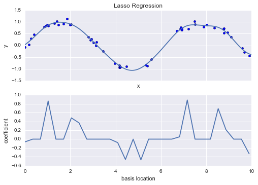
 ) regularization applied to the overly complex model (compare to Figure 5-48)
With the lasso regression penalty, the majority of the coefficients are
exactly zero, with the functional behavior being modeled by a small
subset of the available basis functions. As with ridge
regularization, the  parameter tunes the
strength of the penalty, and should be determined via, for example,
cross-validation (refer back to
“Hyperparameters and Model Validation” for a discussion of this).
parameter tunes the
strength of the penalty, and should be determined via, for example,
cross-validation (refer back to
“Hyperparameters and Model Validation” for a discussion of this).
As an example, let’s take a look at whether we can predict the number of bicycle trips across Seattle’s Fremont Bridge based on weather, season, and other factors. We have seen this data already in “Working with Time Series”.
In this section, we will join the bike data with another dataset, and try to determine the extent to which weather and seasonal factors—temperature, precipitation, and daylight hours—affect the volume of bicycle traffic through this corridor. Fortunately, the NOAA makes available their daily weather station data (I used station ID USW00024233) and we can easily use Pandas to join the two data sources. We will perform a simple linear regression to relate weather and other information to bicycle counts, in order to estimate how a change in any one of these parameters affects the number of riders on a given day.
In particular, this is an example of how the tools of Scikit-Learn can be used in a statistical modeling framework, in which the parameters of the model are assumed to have interpretable meaning. As discussed previously, this is not a standard approach within machine learning, but such interpretation is possible for some models.
Let’s start by loading the two datasets, indexing by date:
In[14]:importpandasaspdcounts=pd.read_csv('fremont_hourly.csv',index_col='Date',parse_dates=True)weather=pd.read_csv('599021.csv',index_col='DATE',parse_dates=True)
Next we will compute the total daily bicycle traffic, and put this in
its own DataFrame:
In[15]:daily=counts.resample('d',how='sum')daily['Total']=daily.sum(axis=1)daily=daily[['Total']]# remove other columns
We saw previously that the patterns of use generally vary from day to day; let’s account for this in our data by adding binary columns that indicate the day of the week:
In[16]:days=['Mon','Tue','Wed','Thu','Fri','Sat','Sun']foriinrange(7):daily[days[i]]=(daily.index.dayofweek==i).astype(float)
Similarly, we might expect riders to behave differently on holidays; let’s add an indicator of this as well:
In[17]:frompandas.tseries.holidayimportUSFederalHolidayCalendarcal=USFederalHolidayCalendar()holidays=cal.holidays('2012','2016')daily=daily.join(pd.Series(1,index=holidays,name='holiday'))daily['holiday'].fillna(0,inplace=True)
We also might suspect that the hours of daylight would affect how many people ride; let’s use the standard astronomical calculation to add this information (Figure 5-51):
In[18]:defhours_of_daylight(date,axis=23.44,latitude=47.61):"""Compute the hours of daylight for the given date"""days=(date-pd.datetime(2000,12,21)).daysm=(1.-np.tan(np.radians(latitude))*np.tan(np.radians(axis)*np.cos(days*2*np.pi/365.25)))return24.*np.degrees(np.arccos(1-np.clip(m,0,2)))/180.daily['daylight_hrs']=list(map(hours_of_daylight,daily.index))daily[['daylight_hrs']].plot();
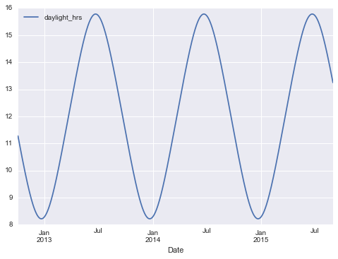
We can also add the average temperature and total precipitation to the data. In addition to the inches of precipitation, let’s add a flag that indicates whether a day is dry (has zero precipitation):
In[19]:# temperatures are in 1/10 deg C; convert to Cweather['TMIN']/=10weather['TMAX']/=10weather['Temp (C)']=0.5*(weather['TMIN']+weather['TMAX'])# precip is in 1/10 mm; convert to inchesweather['PRCP']/=254weather['dry day']=(weather['PRCP']==0).astype(int)daily=daily.join(weather[['PRCP','Temp (C)','dry day']])
Finally, let’s add a counter that increases from day 1, and measures how many years have passed. This will let us measure any observed annual increase or decrease in daily crossings:
In[20]:daily['annual']=(daily.index-daily.index[0]).days/365.
Now our data is in order, and we can take a look at it:
In[21]:daily.head()
Out[21]:
Total Mon Tue Wed Thu Fri Sat Sun holiday daylight_hrs \\
Date
2012-10-03 3521 0 0 1 0 0 0 0 0 11.277359
2012-10-04 3475 0 0 0 1 0 0 0 0 11.219142
2012-10-05 3148 0 0 0 0 1 0 0 0 11.161038
2012-10-06 2006 0 0 0 0 0 1 0 0 11.103056
2012-10-07 2142 0 0 0 0 0 0 1 0 11.045208
PRCP Temp (C) dry day annual
Date
2012-10-03 0 13.35 1 0.000000
2012-10-04 0 13.60 1 0.002740
2012-10-05 0 15.30 1 0.005479
2012-10-06 0 15.85 1 0.008219
2012-10-07 0 15.85 1 0.010959
With this in place, we can choose the columns to use, and fit a linear
regression model to our data. We will set fit_intercept = False,
because the daily flags essentially operate as their own day-specific
intercepts:
In[22]:column_names=['Mon','Tue','Wed','Thu','Fri','Sat','Sun','holiday','daylight_hrs','PRCP','dry day','Temp (C)','annual']X=daily[column_names]y=daily['Total']model=LinearRegression(fit_intercept=False)model.fit(X,y)daily['predicted']=model.predict(X)
Finally, we can compare the total and predicted bicycle traffic visually (Figure 5-52):
In[23]:daily[['Total','predicted']].plot(alpha=0.5);
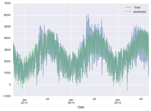
It is evident that we have missed some key features, especially during the summer time. Either our features are not complete (i.e., people decide whether to ride to work based on more than just these) or there are some nonlinear relationships that we have failed to take into account (e.g., perhaps people ride less at both high and low temperatures). Nevertheless, our rough approximation is enough to give us some insights, and we can take a look at the coefficients of the linear model to estimate how much each feature contributes to the daily bicycle count:
In[24]:params=pd.Series(model.coef_,index=X.columns)params
Out[24]: Mon 503.797330
Tue 612.088879
Wed 591.611292
Thu 481.250377
Fri 176.838999
Sat -1104.321406
Sun -1134.610322
holiday -1187.212688
daylight_hrs 128.873251
PRCP -665.185105
dry day 546.185613
Temp (C) 65.194390
annual 27.865349
dtype: float64
These numbers are difficult to interpret without some measure of their uncertainty. We can compute these uncertainties quickly using bootstrap resamplings of the data:
In[25]:fromsklearn.utilsimportresamplenp.random.seed(1)err=np.std([model.fit(*resample(X,y)).coef_foriinrange(1000)],0)
With these errors estimated, let’s again look at the results:
In[26]:(pd.DataFrame({'effect':params.round(0),'error':err.round(0)}))
effect error Mon 504 85 Tue 612 82 Wed 592 82 Thu 481 85 Fri 177 81 Sat -1104 79 Sun -1135 82 holiday -1187 164 daylight_hrs 129 9 PRCP -665 62 dry day 546 33 Temp (C) 65 4 annual 28 18
We first see that there is a relatively stable trend in the weekly baseline: there are many more riders on weekdays than on weekends and holidays. We see that for each additional hour of daylight, 129 ± 9 more people choose to ride; a temperature increase of one degree Celsius encourages 65 ± 4 people to grab their bicycle; a dry day means an average of 546 ± 33 more riders; and each inch of precipitation means 665 ± 62 more people leave their bike at home. Once all these effects are accounted for, we see a modest increase of 28 ± 18 new daily riders each year.
Our model is almost certainly missing some relevant information. For example, nonlinear effects (such as effects of precipitation and cold temperature) and nonlinear trends within each variable (such as disinclination to ride at very cold and very hot temperatures) cannot be accounted for in this model. Additionally, we have thrown away some of the finer-grained information (such as the difference between a rainy morning and a rainy afternoon), and we have ignored correlations between days (such as the possible effect of a rainy Tuesday on Wednesday’s numbers, or the effect of an unexpected sunny day after a streak of rainy days). These are all potentially interesting effects, and you now have the tools to begin exploring them if you wish!
Support vector machines (SVMs) are a particularly powerful and flexible class of supervised algorithms for both classification and regression. In this section, we will develop the intuition behind support vector machines and their use in classification problems. We begin with the standard imports:
In[1]:%matplotlibinlineimportnumpyasnpimportmatplotlib.pyplotaspltfromscipyimportstats# use Seaborn plotting defaultsimportseabornassns;sns.set()
As part of our discussion of Bayesian classification (see “In Depth: Naive Bayes Classification”), we learned a simple model describing the distribution of each underlying class, and used these generative models to probabilistically determine labels for new points. That was an example of generative classification; here we will consider instead discriminative classification: rather than modeling each class, we simply find a line or curve (in two dimensions) or manifold (in multiple dimensions) that divides the classes from each other.
As an example of this, consider the simple case of a classification task, in which the two classes of points are well separated (Figure 5-53):
In[2]:fromsklearn.datasets.samples_generatorimportmake_blobsX,y=make_blobs(n_samples=50,centers=2,random_state=0,cluster_std=0.60)plt.scatter(X[:,0],X[:,1],c=y,s=50,cmap='autumn');
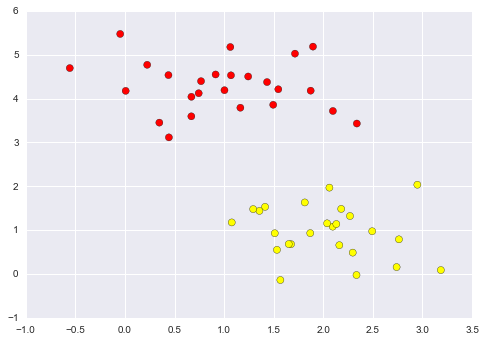
A linear discriminative classifier would attempt to draw a straight line separating the two sets of data, and thereby create a model for classification. For two-dimensional data like that shown here, this is a task we could do by hand. But immediately we see a problem: there is more than one possible dividing line that can perfectly discriminate between the two classes!
We can draw them as follows (Figure 5-54):
In[3]:xfit=np.linspace(-1,3.5)plt.scatter(X[:,0],X[:,1],c=y,s=50,cmap='autumn')plt.plot([0.6],[2.1],'x',color='red',markeredgewidth=2,markersize=10)form,bin[(1,0.65),(0.5,1.6),(-0.2,2.9)]:plt.plot(xfit,m*xfit+b,'-k')plt.xlim(-1,3.5);
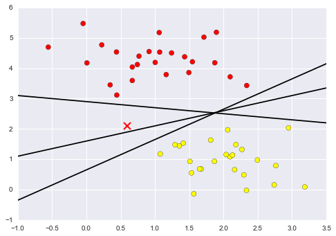
These are three very different separators that, nevertheless, perfectly discriminate between these samples. Depending on which you choose, a new data point (e.g., the one marked by the “X” in Figure 5-54) will be assigned a different label! Evidently our simple intuition of “drawing a line between classes” is not enough, and we need to think a bit deeper.
Support vector machines offer one way to improve on this. The intuition is this: rather than simply drawing a zero-width line between the classes, we can draw around each line a margin of some width, up to the nearest point. Here is an example of how this might look (Figure 5-55):
In[4]:xfit=np.linspace(-1,3.5)plt.scatter(X[:,0],X[:,1],c=y,s=50,cmap='autumn')form,b,din[(1,0.65,0.33),(0.5,1.6,0.55),(-0.2,2.9,0.2)]:yfit=m*xfit+bplt.plot(xfit,yfit,'-k')plt.fill_between(xfit,yfit-d,yfit+d,edgecolor='none',color='#AAAAAA',alpha=0.4)plt.xlim(-1,3.5);
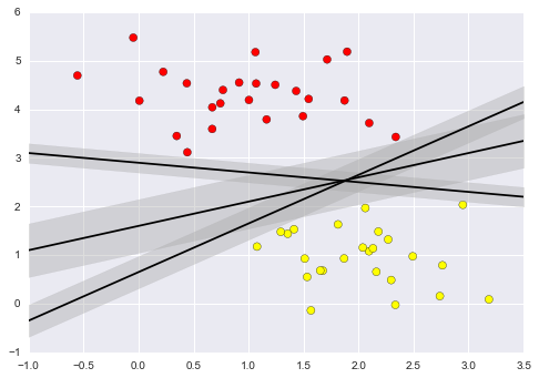
In support vector machines, the line that maximizes this margin is the one we will choose as the optimal model. Support vector machines are an example of such a maximum margin estimator.
Let’s see the result of an actual fit to this data: we will use
Scikit-Learn’s support vector classifier to train an SVM model on this
data. For the time being, we will use a linear kernel and set the C
parameter to a very large number (we’ll discuss the meaning of these in more depth momentarily):
In[5]:fromsklearn.svmimportSVC# "Support vector classifier"model=SVC(kernel='linear',C=1E10)model.fit(X,y)
Out[5]: SVC(C=10000000000.0, cache_size=200, class_weight=None, coef0=0.0,
decision_function_shape=None, degree=3, gamma='auto', kernel='linear',
max_iter=-1, probability=False, random_state=None, shrinking=True,
tol=0.001, verbose=False)
To better visualize what’s happening here, let’s create a quick convenience function that will plot SVM decision boundaries for us (Figure 5-56):
In[6]:defplot_svc_decision_function(model,ax=None,plot_support=True):"""Plot the decision function for a two-dimensional SVC"""ifaxisNone:ax=plt.gca()xlim=ax.get_xlim()ylim=ax.get_ylim()# create grid to evaluate modelx=np.linspace(xlim[0],xlim[1],30)y=np.linspace(ylim[0],ylim[1],30)Y,X=np.meshgrid(y,x)xy=np.vstack([X.ravel(),Y.ravel()]).TP=model.decision_function(xy).reshape(X.shape)# plot decision boundary and marginsax.contour(X,Y,P,colors='k',levels=[-1,0,1],alpha=0.5,linestyles=['--','-','--'])# plot support vectorsifplot_support:ax.scatter(model.support_vectors_[:,0],model.support_vectors_[:,1],s=300,linewidth=1,facecolors='none');ax.set_xlim(xlim)ax.set_ylim(ylim)
In[7]:plt.scatter(X[:,0],X[:,1],c=y,s=50,cmap='autumn')plot_svc_decision_function(model);
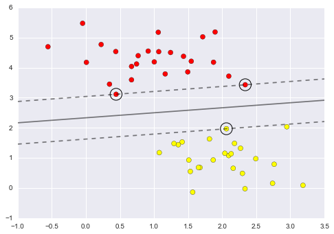
This is the dividing line that maximizes the margin between the two sets
of points. Notice that a few of the training points just touch the
margin; they are indicated by the black circles in Figure 5-56. These
points are the pivotal elements of this fit, and are known as the
support vectors, and give the algorithm its name. In Scikit-Learn, the
identity of these points is stored in the support_vectors_ attribute
of the classifier:
In[8]:model.support_vectors_
Out[8]: array([[ 0.44359863, 3.11530945],
[ 2.33812285, 3.43116792],
[ 2.06156753, 1.96918596]])
A key to this classifier’s success is that for the fit, only the position of the support vectors matters; any points further from the margin that are on the correct side do not modify the fit! Technically, this is because these points do not contribute to the loss function used to fit the model, so their position and number do not matter so long as they do not cross the margin.
We can see this, for example, if we plot the model learned from the first 60 points and first 120 points of this dataset (Figure 5-57):
In[9]:defplot_svm(N=10,ax=None):X,y=make_blobs(n_samples=200,centers=2,random_state=0,cluster_std=0.60)X=X[:N]y=y[:N]model=SVC(kernel='linear',C=1E10)model.fit(X,y)ax=axorplt.gca()ax.scatter(X[:,0],X[:,1],c=y,s=50,cmap='autumn')ax.set_xlim(-1,4)ax.set_ylim(-1,6)plot_svc_decision_function(model,ax)fig,ax=plt.subplots(1,2,figsize=(16,6))fig.subplots_adjust(left=0.0625,right=0.95,wspace=0.1)foraxi,Ninzip(ax,[60,120]):plot_svm(N,axi)axi.set_title('N = {0}'.format(N))
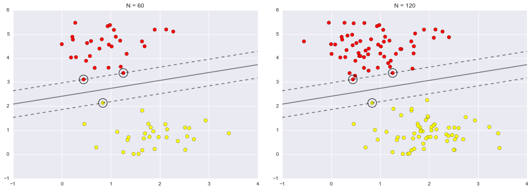
In the left panel, we see the model and the support vectors for 60 training points. In the right panel, we have doubled the number of training points, but the model has not changed: the three support vectors from the left panel are still the support vectors from the right panel. This insensitivity to the exact behavior of distant points is one of the strengths of the SVM model.
If you are running this notebook live, you can use IPython’s interactive widgets to view this feature of the SVM model interactively (Figure 5-58):
In[10]:fromipywidgetsimportinteract,fixedinteract(plot_svm,N=[10,200],ax=fixed(None));
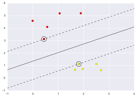
Where SVM becomes extremely powerful is when it is combined with kernels. We have seen a version of kernels before, in the basis function regressions of “In Depth: Linear Regression”. There we projected our data into higher-dimensional space defined by polynomials and Gaussian basis functions, and thereby were able to fit for nonlinear relationships with a linear classifier.
In SVM models, we can use a version of the same idea. To motivate the need for kernels, let’s look at some data that is not linearly separable (Figure 5-59):
In[11]:fromsklearn.datasets.samples_generatorimportmake_circlesX,y=make_circles(100,factor=.1,noise=.1)clf=SVC(kernel='linear').fit(X,y)plt.scatter(X[:,0],X[:,1],c=y,s=50,cmap='autumn')plot_svc_decision_function(clf,plot_support=False);
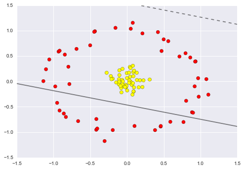
It is clear that no linear discrimination will ever be able to separate this data. But we can draw a lesson from the basis function regressions in “In Depth: Linear Regression”, and think about how we might project the data into a higher dimension such that a linear separator would be sufficient. For example, one simple projection we could use would be to compute a radial basis function centered on the middle clump:
In[12]:r=np.exp(-(X**2).sum(1))
We can visualize this extra data dimension using a three-dimensional plot—if you are running this notebook live, you will be able to use the sliders to rotate the plot (Figure 5-60):
In[13]:frommpl_toolkitsimportmplot3ddefplot_3D(elev=30,azim=30,X=X,y=y):ax=plt.subplot(projection='3d')ax.scatter3D(X[:,0],X[:,1],r,c=y,s=50,cmap='autumn')ax.view_init(elev=elev,azim=azim)ax.set_xlabel('x')ax.set_ylabel('y')ax.set_zlabel('r')interact(plot_3D,elev=[-90,90],azip=(-180,180),X=fixed(X),y=fixed(y));
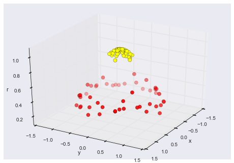
We can see that with this additional dimension, the data becomes trivially linearly separable, by drawing a separating plane at, say, r=0.7.
Here we had to choose and carefully tune our projection; if we had not centered our radial basis function in the right location, we would not have seen such clean, linearly separable results. In general, the need to make such a choice is a problem: we would like to somehow automatically find the best basis functions to use.
One strategy to this end is to compute a basis function centered at every point in the dataset, and let the SVM algorithm sift through the results. This type of basis function transformation is known as a kernel transformation, as it is based on a similarity relationship (or kernel) between each pair of points.
A potential problem with this strategy—projecting  points into
  dimensions—is that it might become very
computationally intensive as
dimensions—is that it might become very
computationally intensive as  grows large. However,
because of a neat little procedure known as the
kernel trick, a fit on
kernel-transformed data can be done implicitly—that is, without ever
building the full
grows large. However,
because of a neat little procedure known as the
kernel trick, a fit on
kernel-transformed data can be done implicitly—that is, without ever
building the full  -dimensional representation of the
kernel projection! This kernel trick is built into the SVM, and is one
of the reasons the method is so powerful.
-dimensional representation of the
kernel projection! This kernel trick is built into the SVM, and is one
of the reasons the method is so powerful.
In Scikit-Learn, we can apply kernelized SVM simply by changing our
linear kernel to an RBF (radial basis function) kernel, using the
kernel model hyperparameter (Figure 5-61):
In[14]:clf=SVC(kernel='rbf',C=1E6)clf.fit(X,y)
Out[14]: SVC(C=1000000.0, cache_size=200, class_weight=None, coef0=0.0,
decision_function_shape=None, degree=3, gamma='auto', kernel='rbf',
max_iter=-1, probability=False, random_state=None, shrinking=True,
tol=0.001, verbose=False)
In[15]:plt.scatter(X[:,0],X[:,1],c=y,s=50,cmap='autumn')plot_svc_decision_function(clf)plt.scatter(clf.support_vectors_[:,0],clf.support_vectors_[:,1],s=300,lw=1,facecolors='none');
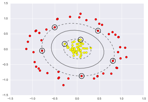
Using this kernelized support vector machine, we learn a suitable nonlinear decision boundary. This kernel transformation strategy is used often in machine learning to turn fast linear methods into fast nonlinear methods, especially for models in which the kernel trick can be used.
Our discussion so far has centered on very clean datasets, in which a perfect decision boundary exists. But what if your data has some amount of overlap? For example, you may have data like this (Figure 5-62):
In[16]:X,y=make_blobs(n_samples=100,centers=2,random_state=0,cluster_std=1.2)plt.scatter(X[:,0],X[:,1],c=y,s=50,cmap='autumn');
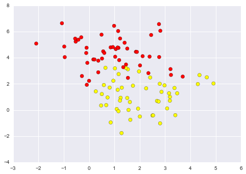
To handle this case, the SVM implementation has a bit of a fudge-factor
that “softens” the margin; that is, it allows some of the points to
creep into the margin if that allows a better fit. The hardness of the
margin is controlled by a tuning parameter, most often known as
 . For very large
  , the margin is hard, and
points cannot lie in it. For smaller
, the margin is hard, and
points cannot lie in it. For smaller  , the margin is
softer, and can grow to encompass some points.
, the margin is
softer, and can grow to encompass some points.
The plot shown in Figure 5-63 gives a visual picture of how a changing
 parameter affects the final fit, via the softening of
the margin:
parameter affects the final fit, via the softening of
the margin:
In[17]:X,y=make_blobs(n_samples=100,centers=2,random_state=0,cluster_std=0.8)fig,ax=plt.subplots(1,2,figsize=(16,6))fig.subplots_adjust(left=0.0625,right=0.95,wspace=0.1)foraxi,Cinzip(ax,[10.0,0.1]):model=SVC(kernel='linear',C=C).fit(X,y)axi.scatter(X[:,0],X[:,1],c=y,s=50,cmap='autumn')plot_svc_decision_function(model,axi)axi.scatter(model.support_vectors_[:,0],model.support_vectors_[:,1],s=300,lw=1,facecolors='none');axi.set_title('C = {0:.1f}'.format(C),size=14)
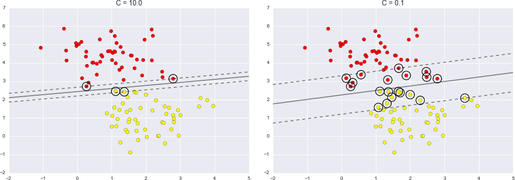
The optimal value of the  parameter will depend on your
dataset, and should be tuned via cross-validation or a similar
procedure (refer back to “Hyperparameters and Model Validation” for further information).
parameter will depend on your
dataset, and should be tuned via cross-validation or a similar
procedure (refer back to “Hyperparameters and Model Validation” for further information).
As an example of support vector machines in action, let’s take a look at the facial recognition problem. We will use the Labeled Faces in the Wild dataset, which consists of several thousand collated photos of various public figures. A fetcher for the dataset is built into Scikit-Learn:
In[18]:fromsklearn.datasetsimportfetch_lfw_peoplefaces=fetch_lfw_people(min_faces_per_person=60)(faces.target_names)(faces.images.shape)
['Ariel Sharon' 'Colin Powell' 'Donald Rumsfeld' 'George W Bush' 'Gerhard Schroeder' 'Hugo Chavez' 'Junichiro Koizumi' 'Tony Blair'] (1348, 62, 47)
Let’s plot a few of these faces to see what we’re working with (Figure 5-64):
In[19]:fig,ax=plt.subplots(3,5)fori,axiinenumerate(ax.flat):axi.imshow(faces.images[i],cmap='bone')axi.set(xticks=[],yticks=[],xlabel=faces.target_names[faces.target[i]])
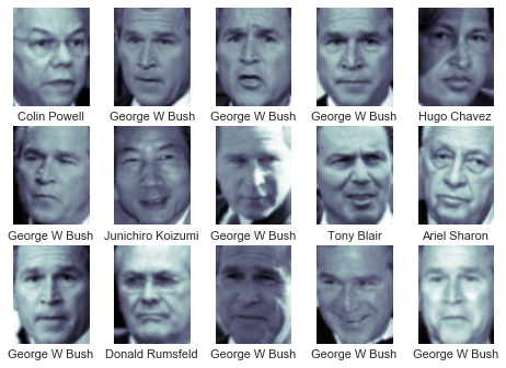
Each image contains [62×47] or nearly 3,000 pixels. We could proceed by simply using each pixel value as a feature, but often it is more effective to use some sort of preprocessor to extract more meaningful features; here we will use a principal component analysis (see “In Depth: Principal Component Analysis”) to extract 150 fundamental components to feed into our support vector machine classifier. We can do this most straightforwardly by packaging the preprocessor and the classifier into a single pipeline:
In[20]:fromsklearn.svmimportSVCfromsklearn.decompositionimportRandomizedPCAfromsklearn.pipelineimportmake_pipelinepca=RandomizedPCA(n_components=150,whiten=True,random_state=42)svc=SVC(kernel='rbf',class_weight='balanced')model=make_pipeline(pca,svc)
For the sake of testing our classifier output, we will split the data into a training and testing set:
In[21]:fromsklearn.cross_validationimporttrain_test_splitXtrain,Xtest,ytrain,ytest=train_test_split(faces.data,faces.target,random_state=42)
Finally, we can use a grid search cross-validation to explore
combinations of parameters. Here we will adjust C (which controls the
margin hardness) and gamma (which controls the size of the radial
basis function kernel), and determine the best model:
In[22]:fromsklearn.grid_searchimportGridSearchCVparam_grid={'svc__C':[1,5,10,50],'svc__gamma':[0.0001,0.0005,0.001,0.005]}grid=GridSearchCV(model,param_grid)%timegrid.fit(Xtrain,ytrain)(grid.best_params_)
CPU times: user 47.8 s, sys: 4.08 s, total: 51.8 s
Wall time: 26 s
{'svc__gamma': 0.001, 'svc__C': 10}
The optimal values fall toward the middle of our grid; if they fell at the edges, we would want to expand the grid to make sure we have found the true optimum.
Now with this cross-validated model, we can predict the labels for the test data, which the model has not yet seen:
In[23]:model=grid.best_estimator_yfit=model.predict(Xtest)
Let’s take a look at a few of the test images along with their predicted values (Figure 5-65):
In[24]:fig,ax=plt.subplots(4,6)fori,axiinenumerate(ax.flat):axi.imshow(Xtest[i].reshape(62,47),cmap='bone')axi.set(xticks=[],yticks=[])axi.set_ylabel(faces.target_names[yfit[i]].split()[-1],color='black'ifyfit[i]==ytest[i]else'red')fig.suptitle('Predicted Names; Incorrect Labels in Red',size=14);
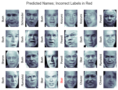
Out of this small sample, our optimal estimator mislabeled only a single face (Bush’s face in the bottom row was mislabeled as Blair). We can get a better sense of our estimator’s performance using the classification report, which lists recovery statistics label by label:
In[25]:fromsklearn.metricsimportclassification_report(classification_report(ytest,yfit,target_names=faces.target_names))
precision recall f1-score support
Ariel Sharon 0.65 0.73 0.69 15
Colin Powell 0.81 0.87 0.84 68
Donald Rumsfeld 0.75 0.87 0.81 31
George W Bush 0.93 0.83 0.88 126
Gerhard Schroeder 0.86 0.78 0.82 23
Hugo Chavez 0.93 0.70 0.80 20
Junichiro Koizumi 0.80 1.00 0.89 12
Tony Blair 0.83 0.93 0.88 42
avg / total 0.85 0.85 0.85 337
We might also display the confusion matrix between these classes (Figure 5-66):
In[26]:fromsklearn.metricsimportconfusion_matrixmat=confusion_matrix(ytest,yfit)sns.heatmap(mat.T,square=True,annot=True,fmt='d',cbar=False,xticklabels=faces.target_names,yticklabels=faces.target_names)plt.xlabel('true label')plt.ylabel('predicted label');
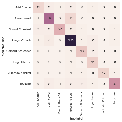
This helps us get a sense of which labels are likely to be confused by the estimator.
For a real-world facial recognition task, in which the photos do not come precropped into nice grids, the only difference in the facial classification scheme is the feature selection: you would need to use a more sophisticated algorithm to find the faces, and extract features that are independent of the pixellation. For this kind of application, one good option is to make use of OpenCV, which among other things, includes pretrained implementations of state-of-the-art feature extraction tools for images in general and faces in particular.
We have seen here a brief intuitive introduction to the principals behind support vector machines. These methods are a powerful classification method for a number of reasons:
Their dependence on relatively few support vectors means that they are very compact models, and take up very little memory.
Once the model is trained, the prediction phase is very fast.
Because they are affected only by points near the margin, they work well with high-dimensional data—even data with more dimensions than samples, which is a challenging regime for other algorithms.
Their integration with kernel methods makes them very versatile, able to adapt to many types of data.
However, SVMs have several disadvantages as well:
The scaling with the number of samples  is
is
 at worst, or
 for efficient implementations. For large
numbers of training samples, this computational cost can be prohibitive.
for efficient implementations. For large
numbers of training samples, this computational cost can be prohibitive.
The results are strongly dependent on a suitable choice for the
softening parameter  . This must be carefully chosen via
cross-validation, which can be expensive as datasets grow in size.
. This must be carefully chosen via
cross-validation, which can be expensive as datasets grow in size.
The results do not have a direct probabilistic interpretation. This
can be estimated via an internal cross-validation (see the probability
parameter of SVC), but this extra estimation is costly.
With those traits in mind, I generally only turn to SVMs once other simpler, faster, and less tuning-intensive methods have been shown to be insufficient for my needs. Nevertheless, if you have the CPU cycles to commit to training and cross-validating an SVM on your data, the method can lead to excellent results.
Previously we have looked in depth at a simple generative classifier (naive Bayes; see “In Depth: Naive Bayes Classification”) and a powerful discriminative classifier (support vector machines; see “In-Depth: Support Vector Machines”). Here we’ll take a look at motivating another powerful algorithm—a nonparametric algorithm called random forests. Random forests are an example of an ensemble method, a method that relies on aggregating the results of an ensemble of simpler estimators. The somewhat surprising result with such ensemble methods is that the sum can be greater than the parts; that is, a majority vote among a number of estimators can end up being better than any of the individual estimators doing the voting! We will see examples of this in the following sections. We begin with the standard imports:
In[1]:%matplotlibinlineimportnumpyasnpimportmatplotlib.pyplotaspltimportseabornassns;sns.set()
Random forests are an example of an ensemble learner built on decision trees. For this reason we’ll start by discussing decision trees themselves.
Decision trees are extremely intuitive ways to classify or label objects: you simply ask a series of questions designed to zero in on the classification. For example, if you wanted to build a decision tree to classify an animal you come across while on a hike, you might construct the one shown in Figure 5-67.
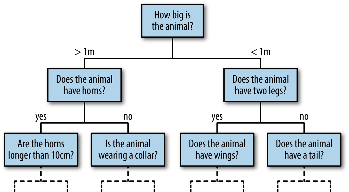
The binary splitting makes this extremely efficient: in a well-constructed tree, each question will cut the number of options by approximately half, very quickly narrowing the options even among a large number of classes. The trick, of course, comes in deciding which questions to ask at each step. In machine learning implementations of decision trees, the questions generally take the form of axis-aligned splits in the data; that is, each node in the tree splits the data into two groups using a cutoff value within one of the features. Let’s now take a look at an example.
Consider the following two-dimensional data, which has one of four class labels (Figure 5-68):
In[2]:fromsklearn.datasetsimportmake_blobsX,y=make_blobs(n_samples=300,centers=4,random_state=0,cluster_std=1.0)plt.scatter(X[:,0],X[:,1],c=y,s=50,cmap='rainbow');
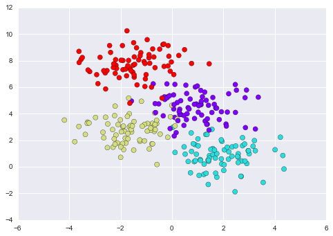
A simple decision tree built on this data will iteratively split the data along one or the other axis according to some quantitative criterion, and at each level assign the label of the new region according to a majority vote of points within it. Figure 5-69 presents a visualization of the first four levels of a decision tree classifier for this data.
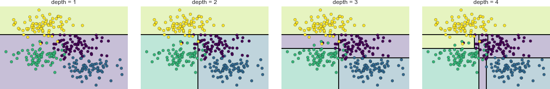
Notice that after the first split, every point in the upper branch remains unchanged, so there is no need to further subdivide this branch. Except for nodes that contain all of one color, at each level every region is again split along one of the two features.
This process of fitting a decision tree to our data can be done in
Scikit-Learn with the DecisionTreeClassifier estimator:
In[3]:fromsklearn.treeimportDecisionTreeClassifiertree=DecisionTreeClassifier().fit(X,y)
Let’s write a quick utility function to help us visualize the output of the classifier:
In[4]:defvisualize_classifier(model,X,y,ax=None,cmap='rainbow'):ax=axorplt.gca()# Plot the training pointsax.scatter(X[:,0],X[:,1],c=y,s=30,cmap=cmap,clim=(y.min(),y.max()),zorder=3)ax.axis('tight')ax.axis('off')xlim=ax.get_xlim()ylim=ax.get_ylim()# fit the estimatormodel.fit(X,y)xx,yy=np.meshgrid(np.linspace(*xlim,num=200),np.linspace(*ylim,num=200))Z=model.predict(np.c_[xx.ravel(),yy.ravel()]).reshape(xx.shape)# Create a color plot with the resultsn_classes=len(np.unique(y))contours=ax.contourf(xx,yy,Z,alpha=0.3,levels=np.arange(n_classes+1)-0.5,cmap=cmap,clim=(y.min(),y.max()),zorder=1)ax.set(xlim=xlim,ylim=ylim)
Now we can examine what the decision tree classification looks like (Figure 5-70):
In[5]:visualize_classifier(DecisionTreeClassifier(),X,y)
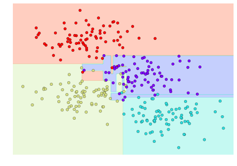
If you’re running this notebook live, you can use the helpers script included in the online appendix to bring up an interactive visualization of the decision tree building process (Figure 5-71):
In[6]:# helpers_05_08 is found in the online appendix# (https://github.com/jakevdp/PythonDataScienceHandbook)importhelpers_05_08helpers_05_08.plot_tree_interactive(X,y);
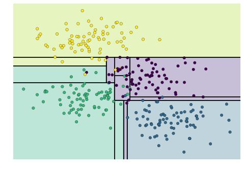
Notice that as the depth increases, we tend to get very strangely shaped classification regions; for example, at a depth of five, there is a tall and skinny purple region between the yellow and blue regions. It’s clear that this is less a result of the true, intrinsic data distribution, and more a result of the particular sampling or noise properties of the data. That is, this decision tree, even at only five levels deep, is clearly overfitting our data.
Such overfitting turns out to be a general property of decision trees; it is very easy to go too deep in the tree, and thus to fit details of the particular data rather than the overall properties of the distributions they are drawn from. Another way to see this overfitting is to look at models trained on different subsets of the data—for example, in Figure 5-72 we train two different trees, each on half of the original data.
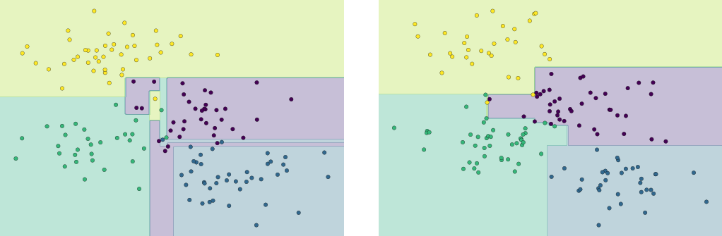
It is clear that in some places, the two trees produce consistent results (e.g., in the four corners), while in other places, the two trees give very different classifications (e.g., in the regions between any two clusters). The key observation is that the inconsistencies tend to happen where the classification is less certain, and thus by using information from both of these trees, we might come up with a better result!
If you are running this notebook live, the following function will allow you to interactively display the fits of trees trained on a random subset of the data (Figure 5-73):
In[7]:# helpers_05_08 is found in the online appendix# (https://github.com/jakevdp/PythonDataScienceHandbook)importhelpers_05_08helpers_05_08.randomized_tree_interactive(X,y)
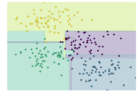
Just as using information from two trees improves our results, we might expect that using information from many trees would improve our results even further.
This notion—that multiple overfitting estimators can be combined to reduce the effect of this overfitting—is what underlies an ensemble method called bagging. Bagging makes use of an ensemble (a grab bag, perhaps) of parallel estimators, each of which overfits the data, and averages the results to find a better classification. An ensemble of randomized decision trees is known as a random forest.
We can do this type of bagging classification manually using
Scikit-Learn’s BaggingClassifier meta-estimator as shown here (Figure 5-74):
In[8]:fromsklearn.treeimportDecisionTreeClassifierfromsklearn.ensembleimportBaggingClassifiertree=DecisionTreeClassifier()bag=BaggingClassifier(tree,n_estimators=100,max_samples=0.8,random_state=1)bag.fit(X,y)visualize_classifier(bag,X,y)

In this example, we have randomized the data by fitting each estimator with a random subset of 80% of the training points. In practice, decision trees are more effectively randomized when some stochasticity is injected in how the splits are chosen; this way, all the data contributes to the fit each time, but the results of the fit still have the desired randomness. For example, when determining which feature to split on, the randomized tree might select from among the top several features. You can read more technical details about these randomization strategies in the Scikit-Learn documentation and references within.
In Scikit-Learn, such an optimized ensemble of randomized decision trees
is implemented in the RandomForestClassifier estimator, which takes
care of all the randomization automatically. All you need to do is
select a number of estimators, and it will very quickly (in parallel, if
desired) fit the ensemble of trees (Figure 5-75):
In[9]:fromsklearn.ensembleimportRandomForestClassifiermodel=RandomForestClassifier(n_estimators=100,random_state=0)visualize_classifier(model,X,y);
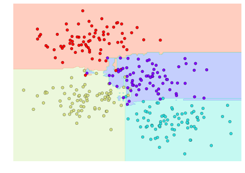
We see that by averaging over 100 randomly perturbed models, we end up with an overall model that is much closer to our intuition about how the parameter space should be split.
In the previous section we considered random forests within the context of
classification. Random forests can also be made to work in the case of
regression (that is, continuous rather than categorical variables). The
estimator to use for this is the RandomForestRegressor, and the syntax
is very similar to what we saw earlier.
Consider the following data, drawn from the combination of a fast and slow oscillation (Figure 5-76):
In[10]:rng=np.random.RandomState(42)x=10*rng.rand(200)defmodel(x,sigma=0.3):fast_oscillation=np.sin(5*x)slow_oscillation=np.sin(0.5*x)noise=sigma*rng.randn(len(x))returnslow_oscillation+fast_oscillation+noisey=model(x)plt.errorbar(x,y,0.3,fmt='o');
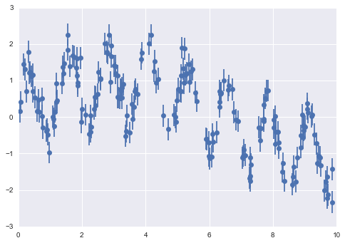
Using the random forest regressor, we can find the best-fit curve as follows (Figure 5-77):
In[11]:fromsklearn.ensembleimportRandomForestRegressorforest=RandomForestRegressor(200)forest.fit(x[:,None],y)xfit=np.linspace(0,10,1000)yfit=forest.predict(xfit[:,None])ytrue=model(xfit,sigma=0)plt.errorbar(x,y,0.3,fmt='o',alpha=0.5)plt.plot(xfit,yfit,'-r');plt.plot(xfit,ytrue,'-k',alpha=0.5);
Here the true model is shown by the smooth curve, while the random forest model is shown by the jagged curve. As you can see, the nonparametric random forest model is flexible enough to fit the multiperiod data, without us needing to specify a multiperiod model!
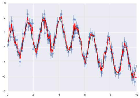
Earlier we took a quick look at the handwritten digits data (see “Introducing Scikit-Learn”). Let’s use that again here to see how the random forest classifier can be used in this context.
In[12]:fromsklearn.datasetsimportload_digitsdigits=load_digits()digits.keys()
Out[12]: dict_keys(['target', 'data', 'target_names', 'DESCR', 'images'])
To remind us what we’re looking at, we’ll visualize the first few data points (Figure 5-78):
In[13]:# set up the figurefig=plt.figure(figsize=(6,6))# figure size in inchesfig.subplots_adjust(left=0,right=1,bottom=0,top=1,hspace=0.05,wspace=0.05)# plot the digits: each image is 8x8 pixelsforiinrange(64):ax=fig.add_subplot(8,8,i+1,xticks=[],yticks=[])ax.imshow(digits.images[i],cmap=plt.cm.binary,interpolation='nearest')# label the image with the target valueax.text(0,7,str(digits.target[i]))
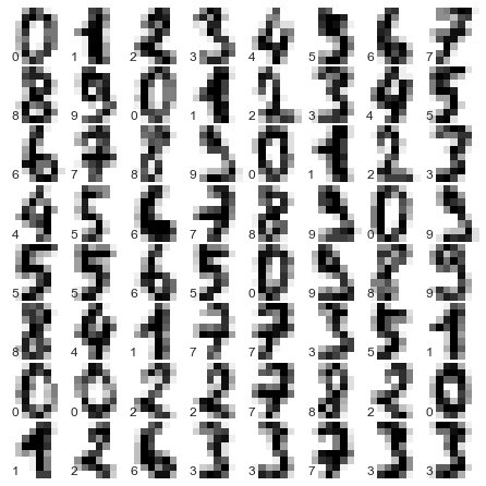
We can quickly classify the digits using a random forest as follows (Figure 5-79):
In[14]:fromsklearn.cross_validationimporttrain_test_splitXtrain,Xtest,ytrain,ytest=train_test_split(digits.data,digits.target,random_state=0)model=RandomForestClassifier(n_estimators=1000)model.fit(Xtrain,ytrain)ypred=model.predict(Xtest)
We can take a look at the classification report for this classifier:
In[15]:fromsklearnimportmetrics(metrics.classification_report(ypred,ytest))
precision recall f1-score support
0 1.00 0.97 0.99 38
1 1.00 0.98 0.99 44
2 0.95 1.00 0.98 42
3 0.98 0.96 0.97 46
4 0.97 1.00 0.99 37
5 0.98 0.96 0.97 49
6 1.00 1.00 1.00 52
7 1.00 0.96 0.98 50
8 0.94 0.98 0.96 46
9 0.96 0.98 0.97 46
avg / total 0.98 0.98 0.98 450
And for good measure, plot the confusion matrix (Figure 5-79):
In[16]:fromsklearn.metricsimportconfusion_matrixmat=confusion_matrix(ytest,ypred)sns.heatmap(mat.T,square=True,annot=True,fmt='d',cbar=False)plt.xlabel('true label')plt.ylabel('predicted label');
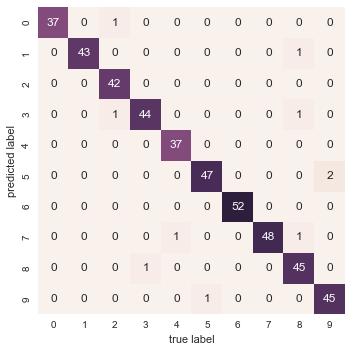
We find that a simple, untuned random forest results in a very accurate classification of the digits data.
This section contained a brief introduction to the concept of ensemble estimators, and in particular the random forest model—an ensemble of randomized decision trees. Random forests are a powerful method with several advantages:
Both training and prediction are very fast, because of the simplicity of the underlying decision trees. In addition, both tasks can be straightforwardly parallelized, because the individual trees are entirely independent entities.
The multiple trees allow for a probabilistic classification: a
majority vote among estimators gives an estimate of the probability
(accessed in Scikit-Learn with the predict_proba() method).
The nonparametric model is extremely flexible, and can thus perform well on tasks that are underfit by other estimators.
A primary disadvantage of random forests is that the results are not easily interpretable; that is, if you would like to draw conclusions about the meaning of the classification model, random forests may not be the best choice.
Up until now, we have been looking in depth at supervised learning estimators: those estimators that predict labels based on labeled training data. Here we begin looking at several unsupervised estimators, which can highlight interesting aspects of the data without reference to any known labels.
In this section, we explore what is perhaps one of the most broadly used of unsupervised algorithms, principal component analysis (PCA). PCA is fundamentally a dimensionality reduction algorithm, but it can also be useful as a tool for visualization, for noise filtering, for feature extraction and engineering, and much more. After a brief conceptual discussion of the PCA algorithm, we will see a couple examples of these further applications. We begin with the standard imports:
In[1]:%matplotlibinlineimportnumpyasnpimportmatplotlib.pyplotaspltimportseabornassns;sns.set()
Principal component analysis is a fast and flexible unsupervised method for dimensionality reduction in data, which we saw briefly in “Introducing Scikit-Learn”. Its behavior is easiest to visualize by looking at a two-dimensional dataset. Consider the following 200 points (Figure 5-80):
In[2]:rng=np.random.RandomState(1)X=np.dot(rng.rand(2,2),rng.randn(2,200)).Tplt.scatter(X[:,0],X[:,1])plt.axis('equal');
By eye, it is clear that there is a nearly linear relationship between the x and y variables. This is reminiscent of the linear regression data we explored in “In Depth: Linear Regression”, but the problem setting here is slightly different: rather than attempting to predict the y values from the x values, the unsupervised learning problem attempts to learn about the relationship between the x and y values.
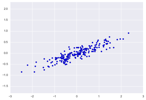
In principal component analysis, one quantifies this relationship by
finding a list of the principal axes in the data, and using those axes
to describe the dataset. Using Scikit-Learn’s PCA estimator, we can
compute this as follows:
In[3]:fromsklearn.decompositionimportPCApca=PCA(n_components=2)pca.fit(X)
Out[3]: PCA(copy=True, n_components=2, whiten=False)
The fit learns some quantities from the data, most importantly the “components” and “explained variance”:
In[4]:(pca.components_)
[[ 0.94446029 0.32862557] [ 0.32862557 -0.94446029]]
In[5]:(pca.explained_variance_)
[ 0.75871884 0.01838551]
To see what these numbers mean, let’s visualize them as vectors over the input data, using the “components” to define the direction of the vector, and the “explained variance” to define the squared-length of the vector (Figure 5-81):
In[6]:defdraw_vector(v0,v1,ax=None):ax=axorplt.gca()arrowprops=dict(arrowstyle='->',linewidth=2,shrinkA=0,shrinkB=0)ax.annotate('',v1,v0,arrowprops=arrowprops)# plot dataplt.scatter(X[:,0],X[:,1],alpha=0.2)forlength,vectorinzip(pca.explained_variance_,pca.components_):v=vector*3*np.sqrt(length)draw_vector(pca.mean_,pca.mean_+v)plt.axis('equal');
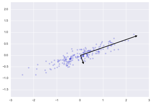
These vectors represent the principal axes of the data, and the length shown in Figure 5-81 is an indication of how “important” that axis is in describing the distribution of the data—more precisely, it is a measure of the variance of the data when projected onto that axis. The projection of each data point onto the principal axes are the “principal components” of the data.
If we plot these principal components beside the original data, we see the plots shown in Figure 5-82.
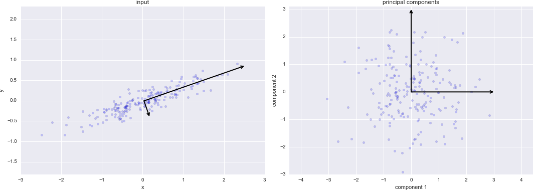
This transformation from data axes to principal axes is as an affine transformation, which basically means it is composed of a translation, rotation, and uniform scaling.
While this algorithm to find principal components may seem like just a mathematical curiosity, it turns out to have very far-reaching applications in the world of machine learning and data exploration.
Using PCA for dimensionality reduction involves zeroing out one or more of the smallest principal components, resulting in a lower-dimensional projection of the data that preserves the maximal data variance.
Here is an example of using PCA as a dimensionality reduction transform:
In[7]:pca=PCA(n_components=1)pca.fit(X)X_pca=pca.transform(X)("original shape: ",X.shape)("transformed shape:",X_pca.shape)
original shape: (200, 2) transformed shape: (200, 1)
The transformed data has been reduced to a single dimension. To understand the effect of this dimensionality reduction, we can perform the inverse transform of this reduced data and plot it along with the original data (Figure 5-83):
In[8]:X_new=pca.inverse_transform(X_pca)plt.scatter(X[:,0],X[:,1],alpha=0.2)plt.scatter(X_new[:,0],X_new[:,1],alpha=0.8)plt.axis('equal');
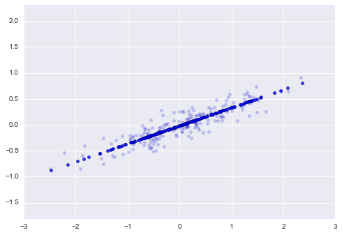
The light points are the original data, while the dark points are the projected version. This makes clear what a PCA dimensionality reduction means: the information along the least important principal axis or axes is removed, leaving only the component(s) of the data with the highest variance. The fraction of variance that is cut out (proportional to the spread of points about the line formed in Figure 5-83) is roughly a measure of how much “information” is discarded in this reduction of dimensionality.
This reduced-dimension dataset is in some senses “good enough” to encode the most important relationships between the points: despite reducing the dimension of the data by 50%, the overall relationship between the data points is mostly preserved.
The usefulness of the dimensionality reduction may not be entirely apparent in only two dimensions, but becomes much more clear when we look at high-dimensional data. To see this, let’s take a quick look at the application of PCA to the digits data we saw in “In-Depth: Decision Trees and Random Forests”.
We start by loading the data:
In[9]:fromsklearn.datasetsimportload_digitsdigits=load_digits()digits.data.shape
Out[9]: (1797, 64)
Recall that the data consists of 8×8 pixel images, meaning that they are 64-dimensional. To gain some intuition into the relationships between these points, we can use PCA to project them to a more manageable number of dimensions, say two:
In[10]:pca=PCA(2)# project from 64 to 2 dimensionsprojected=pca.fit_transform(digits.data)(digits.data.shape)(projected.shape)
(1797, 64) (1797, 2)
We can now plot the first two principal components of each point to learn about the data (Figure 5-84):
In[11]:plt.scatter(projected[:,0],projected[:,1],c=digits.target,edgecolor='none',alpha=0.5,cmap=plt.cm.get_cmap('spectral',10))plt.xlabel('component 1')plt.ylabel('component 2')plt.colorbar();
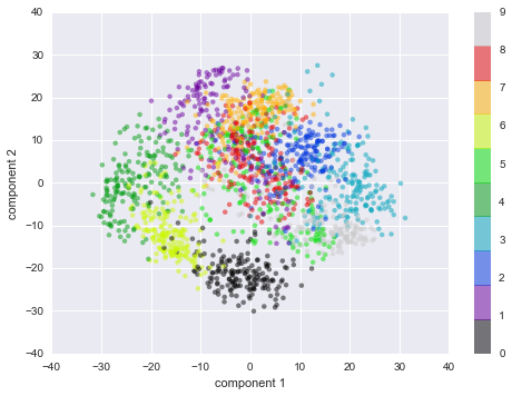
Recall what these components mean: the full data is a 64-dimensional point cloud, and these points are the projection of each data point along the directions with the largest variance. Essentially, we have found the optimal stretch and rotation in 64-dimensional space that allows us to see the layout of the digits in two dimensions, and have done this in an unsupervised manner—that is, without reference to the labels.
We can go a bit further here, and begin to ask what the reduced
dimensions mean. This meaning can be understood in terms of
combinations of basis vectors. For example, each image in the training
set is defined by a collection of 64 pixel values, which we will call
the vector  :
:
One way we can think about this is in terms of a pixel basis. That is, to construct the image, we multiply each element of the vector by the pixel it describes, and then add the results together to build the image:

One way we might imagine reducing the dimension of this data is to zero out all but a few of these basis vectors. For example, if we use only the first eight pixels, we get an eight-dimensional projection of the data (Figure 5-85), but it is not very reflective of the whole image: we’ve thrown out nearly 90% of the pixels!
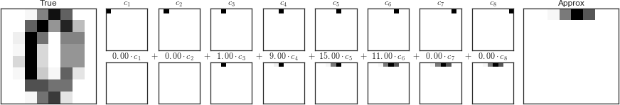
The upper row of panels shows the individual pixels, and the lower row shows the cumulative contribution of these pixels to the construction of the image. Using only eight of the pixel-basis components, we can only construct a small portion of the 64-pixel image. Were we to continue this sequence and use all 64 pixels, we would recover the original image.
But the pixel-wise representation is not the only choice of basis. We can also use other basis functions, which each contain some predefined contribution from each pixel, and write something like:

PCA can be thought of as a process of choosing optimal basis functions, such that adding together just the first few of them is enough to suitably reconstruct the bulk of the elements in the dataset. The principal components, which act as the low-dimensional representation of our data, are simply the coefficients that multiply each of the elements in this series. Figure 5-86 is a similar depiction of reconstructing this digit using the mean plus the first eight PCA basis functions.
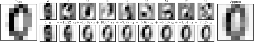
Unlike the pixel basis, the PCA basis allows us to recover the salient features of the input image with just a mean plus eight components! The amount of each pixel in each component is the corollary of the orientation of the vector in our two-dimensional example. This is the sense in which PCA provides a low-dimensional representation of the data: it discovers a set of basis functions that are more efficient than the native pixel-basis of the input data.
A vital part of using PCA in practice is the ability to estimate how many components are needed to describe the data. We can determine this by looking at the cumulative explained variance ratio as a function of the number of components (Figure 5-87):
In[12]:pca=PCA().fit(digits.data)plt.plot(np.cumsum(pca.explained_variance_ratio_))plt.xlabel('number of components')plt.ylabel('cumulative explained variance');
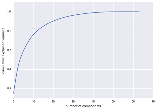
This curve quantifies how much of the total, 64-dimensional variance is
contained within the first  components. For example, we
see that with the digits the first 10 components contain approximately
75% of the variance, while you need around 50 components to describe
close to 100% of the variance.
components. For example, we
see that with the digits the first 10 components contain approximately
75% of the variance, while you need around 50 components to describe
close to 100% of the variance.
Here we see that our two-dimensional projection loses a lot of information (as measured by the explained variance) and that we’d need about 20 components to retain 90% of the variance. Looking at this plot for a high-dimensional dataset can help you understand the level of redundancy present in multiple observations.
PCA can also be used as a filtering approach for noisy data. The idea is this: any components with variance much larger than the effect of the noise should be relatively unaffected by the noise. So if you reconstruct the data using just the largest subset of principal components, you should be preferentially keeping the signal and throwing out the noise.
Let’s see how this looks with the digits data. First we will plot several of the input noise-free data (Figure 5-88):
In[13]:defplot_digits(data):fig,axes=plt.subplots(4,10,figsize=(10,4),subplot_kw={'xticks':[],'yticks':[]},gridspec_kw=dict(hspace=0.1,wspace=0.1))fori,axinenumerate(axes.flat):ax.imshow(data[i].reshape(8,8),cmap='binary',interpolation='nearest',clim=(0,16))plot_digits(digits.data)
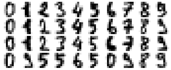
Now let’s add some random noise to create a noisy dataset, and replot it (Figure 5-89):
In[14]:np.random.seed(42)noisy=np.random.normal(digits.data,4)plot_digits(noisy)
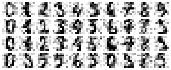
It’s clear by eye that the images are noisy, and contain spurious pixels. Let’s train a PCA on the noisy data, requesting that the projection preserve 50% of the variance:
In[15]:pca=PCA(0.50).fit(noisy)pca.n_components_
Out[15]: 12
Here 50% of the variance amounts to 12 principal components. Now we compute these components, and then use the inverse of the transform to reconstruct the filtered digits (Figure 5-90):
In[16]:components=pca.transform(noisy)filtered=pca.inverse_transform(components)plot_digits(filtered)
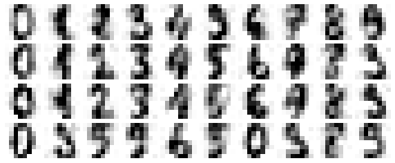
This signal preserving/noise filtering property makes PCA a very useful feature selection routine—for example, rather than training a classifier on very high-dimensional data, you might instead train the classifier on the lower-dimensional representation, which will automatically serve to filter out random noise in the inputs.
Earlier we explored an example of using a PCA projection as a feature selector for facial recognition with a support vector machine (“In-Depth: Support Vector Machines”). Here we will take a look back and explore a bit more of what went into that. Recall that we were using the Labeled Faces in the Wild dataset made available through Scikit-Learn:
In[17]:fromsklearn.datasetsimportfetch_lfw_peoplefaces=fetch_lfw_people(min_faces_per_person=60)(faces.target_names)(faces.images.shape)
['Ariel Sharon' 'Colin Powell' 'Donald Rumsfeld' 'George W Bush' 'Gerhard Schroeder' 'Hugo Chavez' 'Junichiro Koizumi' 'Tony Blair'] (1348, 62, 47)
Let’s take a look at the principal axes that span this dataset. Because
this is a large dataset, we will use RandomizedPCA—it contains a
randomized method to approximate the first  principal
components much more quickly than the standard
principal
components much more quickly than the standard PCA estimator, and thus
is very useful for high-dimensional data (here, a dimensionality of
nearly 3,000). We will take a look at the first 150 components:
In[18]:fromsklearn.decompositionimportRandomizedPCApca=RandomizedPCA(150)pca.fit(faces.data)
Out[18]: RandomizedPCA(copy=True, iterated_power=3, n_components=150,
random_state=None, whiten=False)
In this case, it can be interesting to visualize the images associated with the first several principal components (these components are technically known as “eigenvectors,” so these types of images are often called “eigenfaces”). As you can see in Figure 5-91, they are as creepy as they sound:
In[19]:fig,axes=plt.subplots(3,8,figsize=(9,4),subplot_kw={'xticks':[],'yticks':[]},gridspec_kw=dict(hspace=0.1,wspace=0.1))fori,axinenumerate(axes.flat):ax.imshow(pca.components_[i].reshape(62,47),cmap='bone')
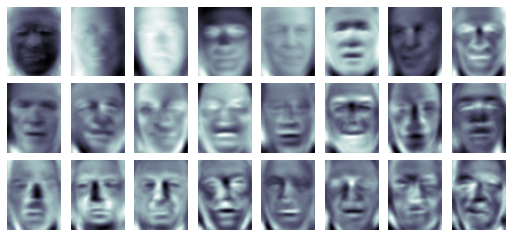
The results are very interesting, and give us insight into how the images vary: for example, the first few eigenfaces (from the top left) seem to be associated with the angle of lighting on the face, and later principal vectors seem to be picking out certain features, such as eyes, noses, and lips. Let’s take a look at the cumulative variance of these components to see how much of the data information the projection is preserving (Figure 5-92):
In[20]:plt.plot(np.cumsum(pca.explained_variance_ratio_))plt.xlabel('number of components')plt.ylabel('cumulative explained variance');
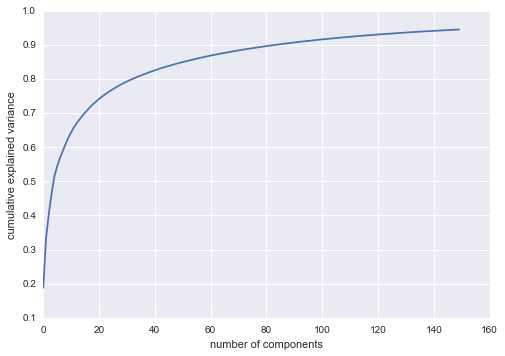
We see that these 150 components account for just over 90% of the variance. That would lead us to believe that using these 150 components, we would recover most of the essential characteristics of the data. To make this more concrete, we can compare the input images with the images reconstructed from these 150 components (Figure 5-93):
In[21]:# Compute the components and projected facespca=RandomizedPCA(150).fit(faces.data)components=pca.transform(faces.data)projected=pca.inverse_transform(components)
In[22]:# Plot the resultsfig,ax=plt.subplots(2,10,figsize=(10,2.5),subplot_kw={'xticks':[],'yticks':[]},gridspec_kw=dict(hspace=0.1,wspace=0.1))foriinrange(10):ax[0,i].imshow(faces.data[i].reshape(62,47),cmap='binary_r')ax[1,i].imshow(projected[i].reshape(62,47),cmap='binary_r')ax[0,0].set_ylabel('full-dim\ninput')ax[1,0].set_ylabel('150-dim\nreconstruction');
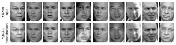
The top row here shows the input images, while the bottom row shows the reconstruction of the images from just 150 of the ~3,000 initial features. This visualization makes clear why the PCA feature selection used in “In-Depth: Support Vector Machines” was so successful: although it reduces the dimensionality of the data by nearly a factor of 20, the projected images contain enough information that we might, by eye, recognize the individuals in the image. What this means is that our classification algorithm needs to be trained on 150-dimensional data rather than 3,000-dimensional data, which depending on the particular algorithm we choose, can lead to a much more efficient classification.
In this section we have discussed the use of principal component analysis for dimensionality reduction, for visualization of high-dimensional data, for noise filtering, and for feature selection within high-dimensional data. Because of the versatility and interpretability of PCA, it has been shown to be effective in a wide variety of contexts and disciplines. Given any high-dimensional dataset, I tend to start with PCA in order to visualize the relationship between points (as we did with the digits), to understand the main variance in the data (as we did with the eigenfaces), and to understand the intrinsic dimensionality (by plotting the explained variance ratio). Certainly PCA is not useful for every high-dimensional dataset, but it offers a straightforward and efficient path to gaining insight into high-dimensional data.
PCA’s main weakness is that it tends to be highly affected by
outliers in the data. For this reason, many robust variants of PCA have
been developed, many of which act to iteratively discard data points
that are poorly described by the initial components. Scikit-Learn
contains a couple interesting variants on PCA, including RandomizedPCA
and SparsePCA, both also in the sklearn.decomposition submodule.
RandomizedPCA, which we saw earlier, uses a nondeterministic method to
quickly approximate the first few principal components in very
high-dimensional data, while SparsePCA introduces a regularization
term (see “In Depth: Linear Regression”) that serves to enforce sparsity of the components.
In the following sections, we will look at other unsupervised learning methods that build on some of the ideas of PCA.
We have seen how principal component analysis can be used in the dimensionality reduction task—reducing the number of features of a dataset while maintaining the essential relationships between the points. While PCA is flexible, fast, and easily interpretable, it does not perform so well when there are nonlinear relationships within the data; we will see some examples of these below.
To address this deficiency, we can turn to a class of methods known as manifold learning—a class of unsupervised estimators that seeks to describe datasets as low-dimensional manifolds embedded in high-dimensional spaces. When you think of a manifold, I’d suggest imagining a sheet of paper: this is a two-dimensional object that lives in our familiar three-dimensional world, and can be bent or rolled in two dimensions. In the parlance of manifold learning, we can think of this sheet as a two-dimensional manifold embedded in three-dimensional space.
Rotating, reorienting, or stretching the piece of paper in three-dimensional space doesn’t change the flat geometry of the paper: such operations are akin to linear embeddings. If you bend, curl, or crumple the paper, it is still a two-dimensional manifold, but the embedding into the three-dimensional space is no longer linear. Manifold learning algorithms would seek to learn about the fundamental two-dimensional nature of the paper, even as it is contorted to fill the three-dimensional space.
Here we will demonstrate a number of manifold methods, going most deeply into a couple techniques: multidimensional scaling (MDS), locally linear embedding (LLE), and isometric mapping (Isomap). We begin with the standard imports:
In[1]:%matplotlibinlineimportmatplotlib.pyplotaspltimportseabornassns;sns.set()importnumpyasnp
To make these concepts more clear, let’s start by generating some two-dimensional data that we can use to define a manifold. Here is a function that will create data in the shape of the word “HELLO”:
In[2]:defmake_hello(N=1000,rseed=42):# Make a plot with "HELLO" text; save as PNGfig,ax=plt.subplots(figsize=(4,1))fig.subplots_adjust(left=0,right=1,bottom=0,top=1)ax.axis('off')ax.text(0.5,0.4,'HELLO',va='center',ha='center',weight='bold',size=85)fig.savefig('hello.png')plt.close(fig)# Open this PNG and draw random points from itfrommatplotlib.imageimportimreaddata=imread('hello.png')[::-1,:,0].Trng=np.random.RandomState(rseed)X=rng.rand(4*N,2)i,j=(X*data.shape).astype(int).Tmask=(data[i,j]<1)X=X[mask]X[:,0]*=(data.shape[0]/data.shape[1])X=X[:N]returnX[np.argsort(X[:,0])]
Let’s call the function and visualize the resulting data (Figure 5-94):
In[3]:X=make_hello(1000)colorize=dict(c=X[:,0],cmap=plt.cm.get_cmap('rainbow',5))plt.scatter(X[:,0],X[:,1],**colorize)plt.axis('equal');
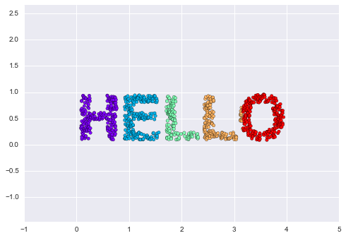
The output is two dimensional, and consists of points drawn in the shape of the word “HELLO”. This data form will help us to see visually what these algorithms are doing.
Looking at data like this, we can see that the particular choice of x and y values of the dataset are not the most fundamental description of the data: we can scale, shrink, or rotate the data, and the “HELLO” will still be apparent. For example, if we use a rotation matrix to rotate the data, the x and y values change, but the data is still fundamentally the same (Figure 5-95):
In[4]:defrotate(X,angle):theta=np.deg2rad(angle)R=[[np.cos(theta),np.sin(theta)],[-np.sin(theta),np.cos(theta)]]returnnp.dot(X,R)X2=rotate(X,20)+5plt.scatter(X2[:,0],X2[:,1],**colorize)plt.axis('equal');
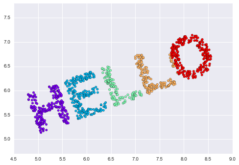
This tells us that the x and y values are not necessarily
fundamental to the relationships in the data. What is fundamental, in
this case, is the distance between each point and the other points in
the dataset. A common way to represent this is to use a distance matrix:
for  points, we construct an
  array such that entry
  contains the distance between
point
contains the distance between
point  and point
  . Let’s use
Scikit-Learn’s efficient
. Let’s use
Scikit-Learn’s efficient pairwise_distances function to do this for
our original data:
In[5]:fromsklearn.metricsimportpairwise_distancesD=pairwise_distances(X)D.shape
Out[5]: (1000, 1000)
As promised, for our N=1,000 points, we obtain a 1,000×1,000 matrix, which can be visualized as shown in Figure 5-96:
In[6]:plt.imshow(D,zorder=2,cmap='Blues',interpolation='nearest')plt.colorbar();
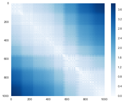
If we similarly construct a distance matrix for our rotated and translated data, we see that it is the same:
In[7]:D2=pairwise_distances(X2)np.allclose(D,D2)
Out[7]: True
This distance matrix gives us a representation of our data that is invariant to rotations and translations, but the visualization of the matrix is not entirely intuitive. In the representation presented in Figure 5-96, we have lost any visible sign of the interesting structure in the data: the “HELLO” that we saw before.
Further, while computing this distance matrix from the (x, y)
coordinates is straightforward, transforming the distances back into x
and y coordinates is rather difficult. This is exactly what the
multidimensional scaling algorithm aims to do: given a distance matrix
between points, it recovers a  -dimensional coordinate
representation of the data. Let’s see how it works for our distance
matrix, using the
-dimensional coordinate
representation of the data. Let’s see how it works for our distance
matrix, using the precomputed dissimilarity to specify that we are
passing a distance matrix (Figure 5-97):
In[8]:fromsklearn.manifoldimportMDSmodel=MDS(n_components=2,dissimilarity='precomputed',random_state=1)out=model.fit_transform(D)plt.scatter(out[:,0],out[:,1],**colorize)plt.axis('equal');
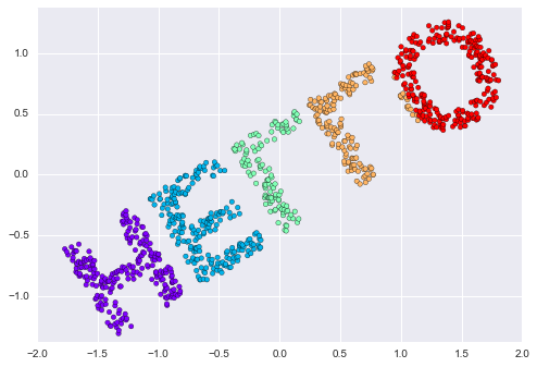
The MDS algorithm recovers one of the possible two-dimensional coordinate
representations of our data, using only the  distance matrix describing the relationship between the data points.
The usefulness of this becomes more apparent when we consider the fact that distance matrices can be computed from data in any dimension. So, for example, instead of simply rotating the data in the two-dimensional plane, we can project it into three dimensions using the following function (essentially a three-dimensional generalization of the rotation matrix used earlier):
In[9]:defrandom_projection(X,dimension=3,rseed=42):assertdimension>=X.shape[1]rng=np.random.RandomState(rseed)C=rng.randn(dimension,dimension)e,V=np.linalg.eigh(np.dot(C,C.T))returnnp.dot(X,V[:X.shape[1]])X3=random_projection(X,3)X3.shape
Out[9]: (1000, 3)
Let’s visualize these points to see what we’re working with (Figure 5-98):
In[10]:frommpl_toolkitsimportmplot3dax=plt.axes(projection='3d')ax.scatter3D(X3[:,0],X3[:,1],X3[:,2],**colorize)ax.view_init(azim=70,elev=50)
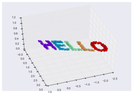
We can now ask the MDS estimator to input this three-dimensional data,
compute the distance matrix, and then determine the optimal
two-dimensional embedding for this distance matrix. The result recovers
a representation of the original data (Figure 5-99):
In[11]:model=MDS(n_components=2,random_state=1)out3=model.fit_transform(X3)plt.scatter(out3[:,0],out3[:,1],**colorize)plt.axis('equal');

This is essentially the goal of a manifold learning estimator: given high-dimensional embedded data, it seeks a low-dimensional representation of the data that preserves certain relationships within the data. In the case of MDS, the quantity preserved is the distance between every pair of points.
Our discussion so far has considered linear embeddings, which essentially consist of rotations, translations, and scalings of data into higher-dimensional spaces. Where MDS breaks down is when the embedding is nonlinear—that is, when it goes beyond this simple set of operations. Consider the following embedding, which takes the input and contorts it into an “S” shape in three dimensions:
In[12]:defmake_hello_s_curve(X):t=(X[:,0]-2)*0.75*np.pix=np.sin(t)y=X[:,1]z=np.sign(t)*(np.cos(t)-1)returnnp.vstack((x,y,z)).TXS=make_hello_s_curve(X)
This is again three-dimensional data, but we can see that the embedding is much more complicated (Figure 5-100):
In[13]:frommpl_toolkitsimportmplot3dax=plt.axes(projection='3d')ax.scatter3D(XS[:,0],XS[:,1],XS[:,2],**colorize);
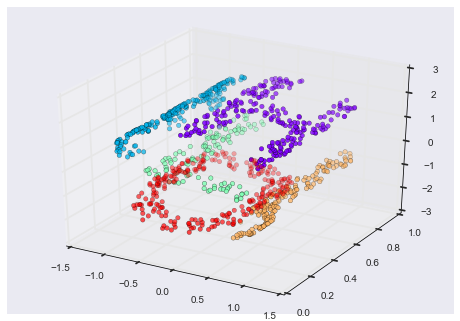
The fundamental relationships between the data points are still there, but this time the data has been transformed in a nonlinear way: it has been wrapped up into the shape of an “S.”
If we try a simple MDS algorithm on this data, it is not able to “unwrap” this nonlinear embedding, and we lose track of the fundamental relationships in the embedded manifold (Figure 5-101):
In[14]:fromsklearn.manifoldimportMDSmodel=MDS(n_components=2,random_state=2)outS=model.fit_transform(XS)plt.scatter(outS[:,0],outS[:,1],**colorize)plt.axis('equal');
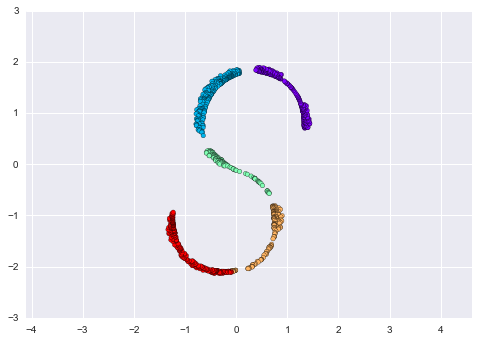
The best two-dimensional linear embedding does not unwrap the S-curve, but instead throws out the original y-axis.
How can we move forward here? Stepping back, we can see that the source of the problem is that MDS tries to preserve distances between faraway points when constructing the embedding. But what if we instead modified the algorithm such that it only preserves distances between nearby points? The resulting embedding would be closer to what we want.
Visually, we can think of it as illustrated in Figure 5-102.
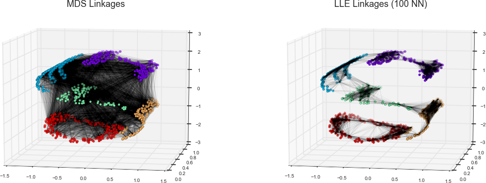
Here each faint line represents a distance that should be preserved in the embedding. On the left is a representation of the model used by MDS: it tries to preserve the distances between each pair of points in the dataset. On the right is a representation of the model used by a manifold learning algorithm called locally linear embedding (LLE): rather than preserving all distances, it instead tries to preserve only the distances between neighboring points: in this case, the nearest 100 neighbors of each point.
Thinking about the left panel, we can see why MDS fails: there is no way to flatten this data while adequately preserving the length of every line drawn between the two points. For the right panel, on the other hand, things look a bit more optimistic. We could imagine unrolling the data in a way that keeps the lengths of the lines approximately the same. This is precisely what LLE does, through a global optimization of a cost function reflecting this logic.
LLE comes in a number of flavors; here we will use the modified LLE algorithm to recover the embedded two-dimensional manifold. In general, modified LLE does better than other flavors of the algorithm at recovering well-defined manifolds with very little distortion (Figure 5-103):
In[15]:fromsklearn.manifoldimportLocallyLinearEmbeddingmodel=LocallyLinearEmbedding(n_neighbors=100,n_components=2,method='modified',eigen_solver='dense')out=model.fit_transform(XS)fig,ax=plt.subplots()ax.scatter(out[:,0],out[:,1],**colorize)ax.set_ylim(0.15,-0.15);
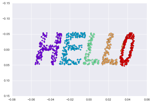
The result remains somewhat distorted compared to our original manifold, but captures the essential relationships in the data!
Though this story and motivation is compelling, in practice manifold learning techniques tend to be finicky enough that they are rarely used for anything more than simple qualitative visualization of high-dimensional data.
The following are some of the particular challenges of manifold learning, which all contrast poorly with PCA:
In manifold learning, there is no good framework for handling missing data. In contrast, there are straightforward iterative approaches for missing data in PCA.
In manifold learning, the presence of noise in the data can “short-circuit” the manifold and drastically change the embedding. In contrast, PCA naturally filters noise from the most important components.
The manifold embedding result is generally highly dependent on the number of neighbors chosen, and there is generally no solid quantitative way to choose an optimal number of neighbors. In contrast, PCA does not involve such a choice.
In manifold learning, the globally optimal number of output dimensions is difficult to determine. In contrast, PCA lets you find the output dimension based on the explained variance.
In manifold learning, the meaning of the embedded dimensions is not always clear. In PCA, the principal components have a very clear meaning.
In manifold learning the computational expense of manifold methods scales as O[N2] or O[N3]. For PCA, there exist randomized approaches that are generally much faster (though see the megaman package for some more scalable implementations of manifold learning).
With all that on the table, the only clear advantage of manifold learning methods over PCA is their ability to preserve nonlinear relationships in the data; for that reason I tend to explore data with manifold methods only after first exploring them with PCA.
Scikit-Learn implements several common variants of manifold learning beyond Isomap and LLE: the Scikit-Learn documentation has a nice discussion and comparison of them. Based on my own experience, I would give the following recommendations:
For toy problems such as the S-curve we saw before, locally linear
embedding (LLE) and its variants (especially modified LLE), perform
very well. This is implemented in
sklearn.manifold.LocallyLinearEmbedding.
For high-dimensional data from real-world sources, LLE often produces
poor results, and isometric mapping (Isomap) seems to generally lead to
more meaningful embeddings. This is implemented in
sklearn.manifold.Isomap.
For data that is highly clustered, t-distributed stochastic neighbor
embedding (t-SNE) seems to work very well, though can be very slow
compared to other methods. This is implemented in
sklearn.manifold.TSNE.
If you’re interested in getting a feel for how these work, I’d suggest running each of the methods on the data in this section.
One place manifold learning is often used is in understanding the relationship between high-dimensional data points. A common case of high-dimensional data is images; for example, a set of images with 1,000 pixels each can be thought of as collection of points in 1,000 dimensions—the brightness of each pixel in each image defines the coordinate in that dimension.
Here let’s apply Isomap on some faces data. We will use the Labeled Faces in the Wild dataset, which we previously saw in “In-Depth: Support Vector Machines” and “In Depth: Principal Component Analysis”. Running this command will download the data and cache it in your home directory for later use:
In[16]:fromsklearn.datasetsimportfetch_lfw_peoplefaces=fetch_lfw_people(min_faces_per_person=30)faces.data.shape
Out[16]: (2370, 2914)
We have 2,370 images, each with 2,914 pixels. In other words, the images can be thought of as data points in a 2,914-dimensional space!
Let’s quickly visualize several of these images to see what we’re working with (Figure 5-104):
In[17]:fig,ax=plt.subplots(4,8,subplot_kw=dict(xticks=[],yticks=[]))fori,axiinenumerate(ax.flat):axi.imshow(faces.images[i],cmap='gray')
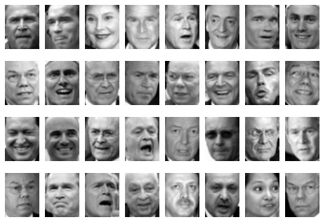
We would like to plot a low-dimensional embedding of the 2,914-dimensional data to learn the fundamental relationships between the images. One useful way to start is to compute a PCA, and examine the explained variance ratio, which will give us an idea of how many linear features are required to describe the data (Figure 5-105):
In[18]:fromsklearn.decompositionimportRandomizedPCAmodel=RandomizedPCA(100).fit(faces.data)plt.plot(np.cumsum(model.explained_variance_ratio_))plt.xlabel('n components')plt.ylabel('cumulative variance');
We see that for this data, nearly 100 components are required to preserve 90% of the variance. This tells us that the data is intrinsically very high dimensional—it can’t be described linearly with just a few components.
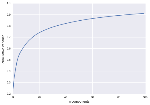
When this is the case, nonlinear manifold embeddings like LLE and Isomap can be helpful. We can compute an Isomap embedding on these faces using the same pattern shown before:
In[19]:fromsklearn.manifoldimportIsomapmodel=Isomap(n_components=2)proj=model.fit_transform(faces.data)proj.shape
Out[19]: (2370, 2)
The output is a two-dimensional projection of all the input images. To get a better idea of what the projection tells us, let’s define a function that will output image thumbnails at the locations of the projections:
In[20]:frommatplotlibimportoffsetboxdefplot_components(data,model,images=None,ax=None,thumb_frac=0.05,cmap='gray'):ax=axorplt.gca()proj=model.fit_transform(data)ax.plot(proj[:,0],proj[:,1],'.k')ifimagesisnotNone:min_dist_2=(thumb_frac*max(proj.max(0)-proj.min(0)))**2shown_images=np.array([2*proj.max(0)])foriinrange(data.shape[0]):dist=np.sum((proj[i]-shown_images)**2,1)ifnp.min(dist)<min_dist_2:# don't show points that are too closecontinueshown_images=np.vstack([shown_images,proj[i]])imagebox=offsetbox.AnnotationBbox(offsetbox.OffsetImage(images[i],cmap=cmap),proj[i])ax.add_artist(imagebox)
Calling this function now, we see the result (Figure 5-106):
In[21]:fig,ax=plt.subplots(figsize=(10,10))plot_components(faces.data,model=Isomap(n_components=2),images=faces.images[:,::2,::2])
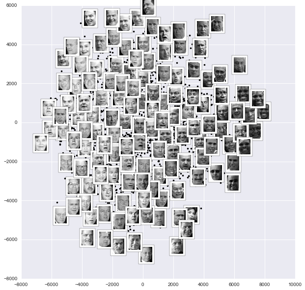
The result is interesting: the first two Isomap dimensions seem to describe global image features: the overall darkness or lightness of the image from left to right, and the general orientation of the face from bottom to top. This gives us a nice visual indication of some of the fundamental features in our data.
We could then go on to classify this data, perhaps using manifold features as inputs to the classification algorithm as we did in “In-Depth: Support Vector Machines”.
As another example of using manifold learning for visualization, let’s take a look at the MNIST handwritten digits set. This data is similar to the digits we saw in “In-Depth: Decision Trees and Random Forests”, but with many more pixels per image. It can be downloaded from http://mldata.org/ with the Scikit-Learn utility:
In[22]:fromsklearn.datasetsimportfetch_mldatamnist=fetch_mldata('MNIST original')mnist.data.shape
Out[22]: (70000, 784)
This consists of 70,000 images, each with 784 pixels (i.e., the images are 28×28). As before, we can take a look at the first few images (Figure 5-107):
In[23]:fig,ax=plt.subplots(6,8,subplot_kw=dict(xticks=[],yticks=[]))fori,axiinenumerate(ax.flat):axi.imshow(mnist.data[1250*i].reshape(28,28),cmap='gray_r')
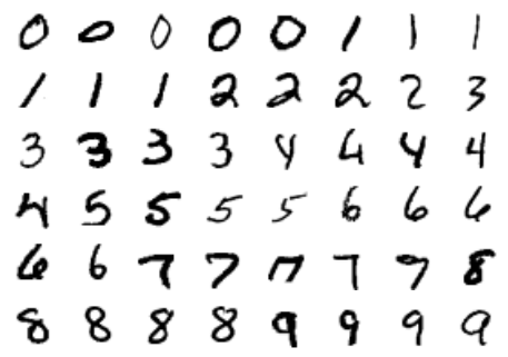
This gives us an idea of the variety of handwriting styles in the dataset.
Let’s compute a manifold learning projection across the data, illustrated in Figure 5-108. For speed here, we’ll only use 1/30 of the data, which is about ~2,000 points (because of the relatively poor scaling of manifold learning, I find that a few thousand samples is a good number to start with for relatively quick exploration before moving to a full calculation):
In[24]:# use only 1/30 of the data: full dataset takes a long time!data=mnist.data[::30]target=mnist.target[::30]model=Isomap(n_components=2)proj=model.fit_transform(data)plt.scatter(proj[:,0],proj[:,1],c=target,cmap=plt.cm.get_cmap('jet',10))plt.colorbar(ticks=range(10))plt.clim(-0.5,9.5);
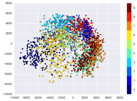
The resulting scatter plot shows some of the relationships between the data points, but is a bit crowded. We can gain more insight by looking at just a single number at a time (Figure 5-109):
In[25]:fromsklearn.manifoldimportIsomap# Choose 1/4 of the "1" digits to projectdata=mnist.data[mnist.target==1][::4]fig,ax=plt.subplots(figsize=(10,10))model=Isomap(n_neighbors=5,n_components=2,eigen_solver='dense')plot_components(data,model,images=data.reshape((-1,28,28)),ax=ax,thumb_frac=0.05,cmap='gray_r')
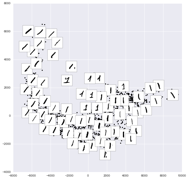
The result gives you an idea of the variety of forms that the number “1” can take within the dataset. The data lies along a broad curve in the projected space, which appears to trace the orientation of the digit. As you move up the plot, you find ones that have hats and/or bases, though these are very sparse within the dataset. The projection lets us identify outliers that have data issues (i.e., pieces of the neighboring digits that snuck into the extracted images).
Now, this in itself may not be useful for the task of classifying digits, but it does help us get an understanding of the data, and may give us ideas about how to move forward, such as how we might want to preprocess the data before building a classification pipeline.
In the previous few sections, we have explored one category of unsupervised machine learning models: dimensionality reduction. Here we will move on to another class of unsupervised machine learning models: clustering algorithms. Clustering algorithms seek to learn, from the properties of the data, an optimal division or discrete labeling of groups of points.
Many clustering algorithms are available in Scikit-Learn and elsewhere,
but perhaps the simplest to understand is an algorithm known as k-means clustering, which is implemented in sklearn.cluster.KMeans. We begin with the standard imports:
In[1]:%matplotlibinlineimportmatplotlib.pyplotaspltimportseabornassns;sns.set()# for plot stylingimportnumpyasnp
The k-means algorithm searches for a predetermined number of clusters within an unlabeled multidimensional dataset. It accomplishes this using a simple conception of what the optimal clustering looks like:
The “cluster center” is the arithmetic mean of all the points belonging to the cluster.
Each point is closer to its own cluster center than to other cluster centers.
Those two assumptions are the basis of the k-means model. We will soon dive into exactly how the algorithm reaches this solution, but for now let’s take a look at a simple dataset and see the k-means result.
First, let’s generate a two-dimensional dataset containing four distinct blobs. To emphasize that this is an unsupervised algorithm, we will leave the labels out of the visualization (Figure 5-110):
In[2]:fromsklearn.datasets.samples_generatorimportmake_blobsX,y_true=make_blobs(n_samples=300,centers=4,cluster_std=0.60,random_state=0)plt.scatter(X[:,0],X[:,1],s=50);
By eye, it is relatively easy to pick out the four clusters. The k-means algorithm does this automatically, and in Scikit-Learn uses the typical estimator API:
In[3]:fromsklearn.clusterimportKMeanskmeans=KMeans(n_clusters=4)kmeans.fit(X)y_kmeans=kmeans.predict(X)
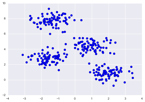
Let’s visualize the results by plotting the data colored by these labels. We will also plot the cluster centers as determined by the k-means estimator (Figure 5-111):
In[4]:plt.scatter(X[:,0],X[:,1],c=y_kmeans,s=50,cmap='viridis')centers=kmeans.cluster_centers_plt.scatter(centers[:,0],centers[:,1],c='black',s=200,alpha=0.5);
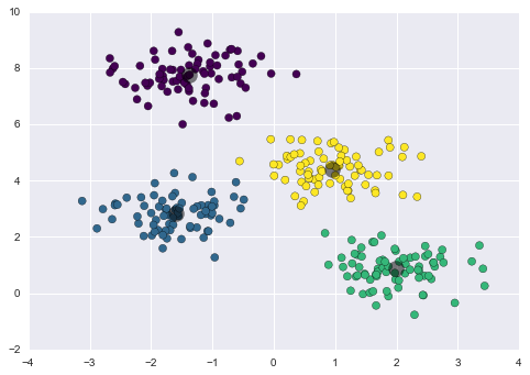
The good news is that the k-means algorithm (at least in this simple case) assigns the points to clusters very similarly to how we might assign them by eye. But you might wonder how this algorithm finds these clusters so quickly! After all, the number of possible combinations of cluster assignments is exponential in the number of data points—an exhaustive search would be very, very costly. Fortunately for us, such an exhaustive search is not necessary; instead, the typical approach to k-means involves an intuitive iterative approach known as expectation–maximization.
Expectation–maximization (E–M) is a powerful algorithm that comes up in a variety of contexts within data science. k-means is a particularly simple and easy-to-understand application of the algorithm, and we will walk through it briefly here. In short, the expectation–maximization approach consists of the following procedure:
Guess some cluster centers
Repeat until converged
E-Step: assign points to the nearest cluster center
M-Step: set the cluster centers to the mean
Here the “E-step” or “Expectation step” is so named because it involves updating our expectation of which cluster each point belongs to. The “M-step” or “Maximization step” is so named because it involves maximizing some fitness function that defines the location of the cluster centers—in this case, that maximization is accomplished by taking a simple mean of the data in each cluster.
The literature about this algorithm is vast, but can be summarized as follows: under typical circumstances, each repetition of the E-step and M-step will always result in a better estimate of the cluster characteristics.
We can visualize the algorithm as shown in Figure 5-112.
For the particular initialization shown here, the clusters converge in just three iterations. For an interactive version of this figure, refer to the code in the online appendix.
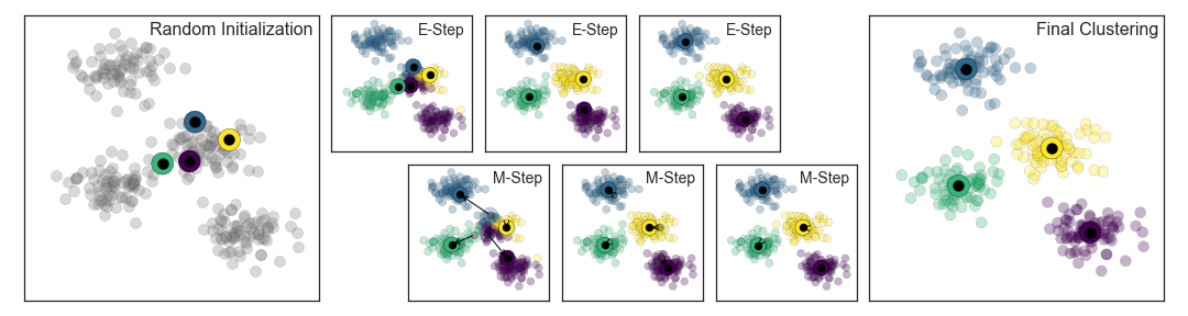
The k-means algorithm is simple enough that we can write it in a few lines of code. The following is a very basic implementation (Figure 5-113):
In[5]:fromsklearn.metricsimportpairwise_distances_argmindeffind_clusters(X,n_clusters,rseed=2):# 1. Randomly choose clustersrng=np.random.RandomState(rseed)i=rng.permutation(X.shape[0])[:n_clusters]centers=X[i]whileTrue:# 2a. Assign labels based on closest centerlabels=pairwise_distances_argmin(X,centers)# 2b. Find new centers from means of pointsnew_centers=np.array([X[labels==i].mean(0)foriinrange(n_clusters)])# 2c. Check for convergenceifnp.all(centers==new_centers):breakcenters=new_centersreturncenters,labelscenters,labels=find_clusters(X,4)plt.scatter(X[:,0],X[:,1],c=labels,s=50,cmap='viridis');
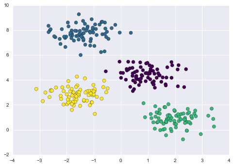
Most well-tested implementations will do a bit more than this under the hood, but the preceding function gives the gist of the expectation–maximization approach.
There are a few issues to be aware of when using the expectation–maximization algorithm.
First, although the E–M procedure is guaranteed to improve the result in each step, there is no assurance that it will lead to the global best solution. For example, if we use a different random seed in our simple procedure, the particular starting guesses lead to poor results (Figure 5-114):
In[6]:centers,labels=find_clusters(X,4,rseed=0)plt.scatter(X[:,0],X[:,1],c=labels,s=50,cmap='viridis');
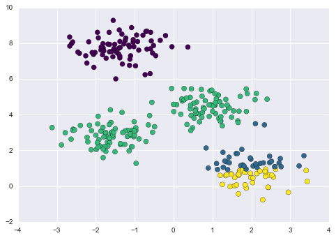
Here the E–M approach has converged, but has not converged to a globally
optimal configuration. For this reason, it is common for the algorithm
to be run for multiple starting guesses, as indeed Scikit-Learn does by
default (set by the n_init parameter, which defaults to 10).
Another common challenge with k-means is that you must tell it how many clusters you expect: it cannot learn the number of clusters from the data. For example, if we ask the algorithm to identify six clusters, it will happily proceed and find the best six clusters (Figure 5-115):
In[7]:labels=KMeans(6,random_state=0).fit_predict(X)plt.scatter(X[:,0],X[:,1],c=labels,s=50,cmap='viridis');
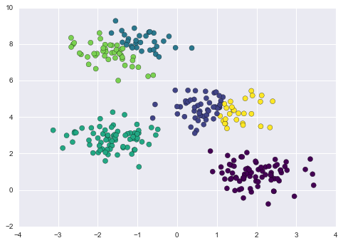
Whether the result is meaningful is a question that is difficult to answer definitively; one approach that is rather intuitive, but that we won’t discuss further here, is called silhouette analysis.
Alternatively, you might use a more complicated clustering algorithm
which has a better quantitative measure of the fitness per number of
clusters (e.g., Gaussian mixture models; see
“In Depth: Gaussian Mixture Models”)
or which can choose a suitable number of clusters (e.g., DBSCAN,
mean-shift, or affinity propagation, all available in the
sklearn.cluster submodule).
The fundamental model assumptions of k-means (points will be closer to their own cluster center than to others) means that the algorithm will often be ineffective if the clusters have complicated geometries.
In particular, the boundaries between k-means clusters will always be linear, which means that it will fail for more complicated boundaries. Consider the following data, along with the cluster labels found by the typical k-means approach (Figure 5-116):
In[8]:fromsklearn.datasetsimportmake_moonsX,y=make_moons(200,noise=.05,random_state=0)
In[9]:labels=KMeans(2,random_state=0).fit_predict(X)plt.scatter(X[:,0],X[:,1],c=labels,s=50,cmap='viridis');
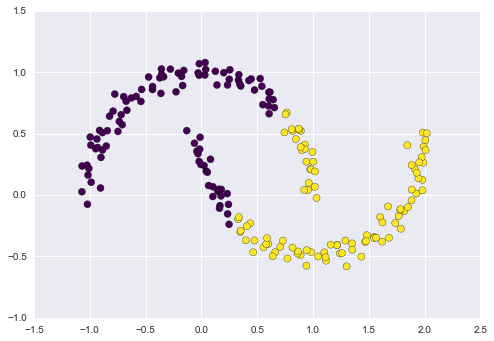
This situation is reminiscent of the discussion in “In-Depth: Support Vector Machines”, where we used a kernel transformation to project the data into a higher dimension where a linear separation is possible. We might imagine using the same trick to allow k-means to discover nonlinear boundaries.
One version of this kernelized k-means is implemented in Scikit-Learn
within the SpectralClustering estimator. It uses the graph of
nearest neighbors to compute a higher-dimensional representation of the
data, and then assigns labels using a k-means algorithm (Figure 5-117):
In[10]:fromsklearn.clusterimportSpectralClusteringmodel=SpectralClustering(n_clusters=2,affinity='nearest_neighbors',assign_labels='kmeans')labels=model.fit_predict(X)plt.scatter(X[:,0],X[:,1],c=labels,s=50,cmap='viridis');
We see that with this kernel transform approach, the kernelized k-means is able to find the more complicated nonlinear boundaries between clusters.
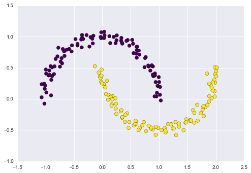
Because each iteration of k-means must access every point in the
dataset, the algorithm can be relatively slow as the number of samples
grows. You might wonder if this requirement to use all data at each
iteration can be relaxed; for example, you might just use a subset of
the data to update the cluster centers at each step. This is the idea
behind batch-based k-means algorithms, one form of which is implemented
in sklearn.cluster.MiniBatchKMeans. The interface for this is the same
as for standard KMeans; we will see an example of its use as we continue our discussion.
Being careful about these limitations of the algorithm, we can use k-means to our advantage in a wide variety of situations. We’ll now take a look at a couple examples.
To start, let’s take a look at applying k-means on the same simple digits data that we saw in “In-Depth: Decision Trees and Random Forests” and “In Depth: Principal Component Analysis”. Here we will attempt to use k-means to try to identify similar digits without using the original label information; this might be similar to a first step in extracting meaning from a new dataset about which you don’t have any a priori label information.
We will start by loading the digits and then finding the KMeans
clusters. Recall that the digits consist of 1,797 samples with 64
features, where each of the 64 features is the brightness of one pixel
in an 8×8 image:
In[11]:fromsklearn.datasetsimportload_digitsdigits=load_digits()digits.data.shape
Out[11]: (1797, 64)
The clustering can be performed as we did before:
In[12]:kmeans=KMeans(n_clusters=10,random_state=0)clusters=kmeans.fit_predict(digits.data)kmeans.cluster_centers_.shape
Out[12]: (10, 64)
The result is 10 clusters in 64 dimensions. Notice that the cluster centers themselves are 64-dimensional points, and can themselves be interpreted as the “typical” digit within the cluster. Let’s see what these cluster centers look like (Figure 5-118):
In[13]:fig,ax=plt.subplots(2,5,figsize=(8,3))centers=kmeans.cluster_centers_.reshape(10,8,8)foraxi,centerinzip(ax.flat,centers):axi.set(xticks=[],yticks=[])axi.imshow(center,interpolation='nearest',cmap=plt.cm.binary)
We see that even without the labels, KMeans is able to find clusters
whose centers are recognizable digits, with perhaps the exception of 1
and 8.
Because k-means knows nothing about the identity of the cluster, the 0–9 labels may be permuted. We can fix this by matching each learned cluster label with the true labels found in them:
In[14]:fromscipy.statsimportmodelabels=np.zeros_like(clusters)foriinrange(10):mask=(clusters==i)labels[mask]=mode(digits.target[mask])[0]
Now we can check how accurate our unsupervised clustering was in finding similar digits within the data:
In[15]:fromsklearn.metricsimportaccuracy_scoreaccuracy_score(digits.target,labels)
Out[15]: 0.79354479688369506
With just a simple k-means algorithm, we discovered the correct grouping for 80% of the input digits! Let’s check the confusion matrix for this (Figure 5-119):
In[16]:fromsklearn.metricsimportconfusion_matrixmat=confusion_matrix(digits.target,labels)sns.heatmap(mat.T,square=True,annot=True,fmt='d',cbar=False,xticklabels=digits.target_names,yticklabels=digits.target_names)plt.xlabel('true label')plt.ylabel('predicted label');
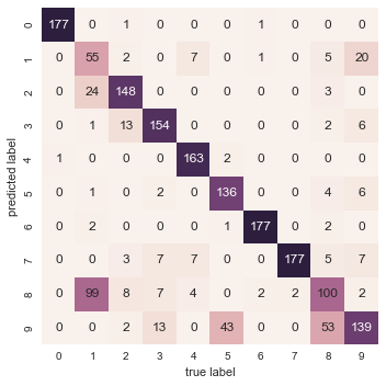
As we might expect from the cluster centers we visualized before, the main point of confusion is between the eights and ones. But this still shows that using k-means, we can essentially build a digit classifier without reference to any known labels!
Just for fun, let’s try to push this even further. We can use the t-distributed stochastic neighbor embedding (t-SNE) algorithm (mentioned in “In-Depth: Manifold Learning”) to preprocess the data before performing k-means. t-SNE is a nonlinear embedding algorithm that is particularly adept at preserving points within clusters. Let’s see how it does:
In[17]:fromsklearn.manifoldimportTSNE# Project the data: this step will take several secondstsne=TSNE(n_components=2,init='pca',random_state=0)digits_proj=tsne.fit_transform(digits.data)# Compute the clusterskmeans=KMeans(n_clusters=10,random_state=0)clusters=kmeans.fit_predict(digits_proj)# Permute the labelslabels=np.zeros_like(clusters)foriinrange(10):mask=(clusters==i)labels[mask]=mode(digits.target[mask])[0]# Compute the accuracyaccuracy_score(digits.target,labels)
Out[17]: 0.93356149137451305
That’s nearly 94% classification accuracy without using the labels. This is the power of unsupervised learning when used carefully: it can extract information from the dataset that it might be difficult to do by hand or by eye.
One interesting application of clustering is in color compression within images. For example, imagine you have an image with millions of colors. In most images, a large number of the colors will be unused, and many of the pixels in the image will have similar or even identical colors.
For example, consider the image shown in Figure 5-120, which is from Scikit-Learn’s datasets module
(for this to work, you’ll have to have the pillow Python package
installed):
In[18]:# Note: this requires the pillow package to be installedfromsklearn.datasetsimportload_sample_imagechina=load_sample_image("china.jpg")ax=plt.axes(xticks=[],yticks=[])ax.imshow(china);
The image itself is stored in a three-dimensional array of size
(height, width, RGB), containing red/blue/green contributions as
integers from 0 to 255:
In[19]:china.shape
Out[19]: (427, 640, 3)

One way we can view this set of pixels is as a cloud of points in a
three-dimensional color space. We will reshape the data to [n_samples x n_features], and rescale the colors so that they lie between 0 and 1:
In[20]:data=china/255.0# use 0...1 scaledata=data.reshape(427*640,3)data.shape
Out[20]: (273280, 3)
We can visualize these pixels in this color space, using a subset of 10,000 pixels for efficiency (Figure 5-121):
In[21]:defplot_pixels(data,title,colors=None,N=10000):ifcolorsisNone:colors=data# choose a random subsetrng=np.random.RandomState(0)i=rng.permutation(data.shape[0])[:N]colors=colors[i]R,G,B=data[i].Tfig,ax=plt.subplots(1,2,figsize=(16,6))ax[0].scatter(R,G,color=colors,marker='.')ax[0].set(xlabel='Red',ylabel='Green',xlim=(0,1),ylim=(0,1))ax[1].scatter(R,B,color=colors,marker='.')ax[1].set(xlabel='Red',ylabel='Blue',xlim=(0,1),ylim=(0,1))fig.suptitle(title,size=20);
In[22]:plot_pixels(data,title='Input color space: 16 million possible colors')
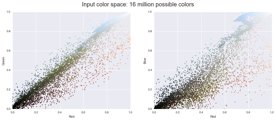
Now let’s reduce these 16 million colors to just 16 colors, using a k-means clustering across the pixel space. Because we are dealing with a very large dataset, we will use the mini batch k-means, which operates on subsets of the data to compute the result much more quickly than the standard k-means algorithm (Figure 5-122):
In[23]:fromsklearn.clusterimportMiniBatchKMeanskmeans=MiniBatchKMeans(16)kmeans.fit(data)new_colors=kmeans.cluster_centers_[kmeans.predict(data)]plot_pixels(data,colors=new_colors,title="Reduced color space: 16 colors")
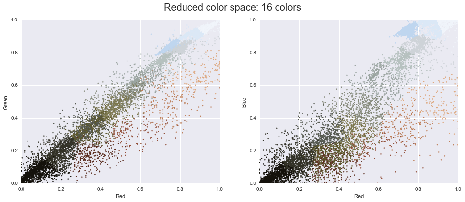
The result is a recoloring of the original pixels, where each pixel is assigned the color of its closest cluster center. Plotting these new colors in the image space rather than the pixel space shows us the effect of this (Figure 5-123):
In[24]:china_recolored=new_colors.reshape(china.shape)fig,ax=plt.subplots(1,2,figsize=(16,6),subplot_kw=dict(xticks=[],yticks=[]))fig.subplots_adjust(wspace=0.05)ax[0].imshow(china)ax[0].set_title('Original Image',size=16)ax[1].imshow(china_recolored)ax[1].set_title('16-color Image',size=16);

Some detail is certainly lost in the rightmost panel, but the overall image is still easily recognizable. This image on the right achieves a compression factor of around 1 million! While this is an interesting application of k-means, there are certainly better way to compress information in images. But the example shows the power of thinking outside of the box with unsupervised methods like k-means.
The k-means clustering model explored in the previous section is simple and relatively easy to understand, but its simplicity leads to practical challenges in its application. In particular, the nonprobabilistic nature of k-means and its use of simple distance-from-cluster-center to assign cluster membership leads to poor performance for many real-world situations. In this section we will take a look at Gaussian mixture models, which can be viewed as an extension of the ideas behind k-means, but can also be a powerful tool for estimation beyond simple clustering. We begin with the standard imports:
In[1]:%matplotlibinlineimportmatplotlib.pyplotaspltimportseabornassns;sns.set()importnumpyasnp
Let’s take a look at some of the weaknesses of k-means and think about how we might improve the cluster model. As we saw in the previous section, given simple, well-separated data, k-means finds suitable clustering results.
For example, if we have simple blobs of data, the k-means algorithm can quickly label those clusters in a way that closely matches what we might do by eye (Figure 5-124):
In[2]:# Generate some datafromsklearn.datasets.samples_generatorimportmake_blobsX,y_true=make_blobs(n_samples=400,centers=4,cluster_std=0.60,random_state=0)X=X[:,::-1]# flip axes for better plotting
In[3]:# Plot the data with k-means labelsfromsklearn.clusterimportKMeanskmeans=KMeans(4,random_state=0)labels=kmeans.fit(X).predict(X)plt.scatter(X[:,0],X[:,1],c=labels,s=40,cmap='viridis');
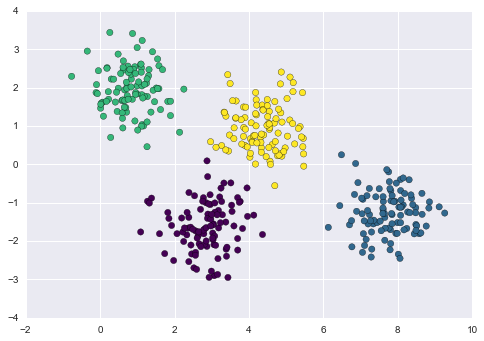
From an intuitive standpoint, we might expect that the clustering assignment for some points is more certain than others; for example, there appears to be a very slight overlap between the two middle clusters, such that we might not have complete confidence in the cluster assignment of points between them. Unfortunately, the k-means model has no intrinsic measure of probability or uncertainty of cluster assignments (although it may be possible to use a bootstrap approach to estimate this uncertainty). For this, we must think about generalizing the model.
One way to think about the k-means model is that it places a circle (or, in higher dimensions, a hyper-sphere) at the center of each cluster, with a radius defined by the most distant point in the cluster. This radius acts as a hard cutoff for cluster assignment within the training set: any point outside this circle is not considered a member of the cluster. We can visualize this cluster model with the following function (Figure 5-125):
In[4]:fromsklearn.clusterimportKMeansfromscipy.spatial.distanceimportcdistdefplot_kmeans(kmeans,X,n_clusters=4,rseed=0,ax=None):labels=kmeans.fit_predict(X)# plot the input dataax=axorplt.gca()ax.axis('equal')ax.scatter(X[:,0],X[:,1],c=labels,s=40,cmap='viridis',zorder=2)# plot the representation of the k-means modelcenters=kmeans.cluster_centers_radii=[cdist(X[labels==i],[center]).max()fori,centerinenumerate(centers)]forc,rinzip(centers,radii):ax.add_patch(plt.Circle(c,r,fc='#CCCCCC',lw=3,alpha=0.5,zorder=1))
In[5]:kmeans=KMeans(n_clusters=4,random_state=0)plot_kmeans(kmeans,X)
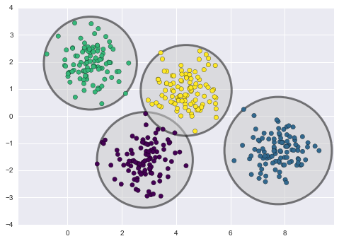
An important observation for k-means is that these cluster models must be circular: k-means has no built-in way of accounting for oblong or elliptical clusters. So, for example, if we take the same data and transform it, the cluster assignments end up becoming muddled (Figure 5-126):
In[6]:rng=np.random.RandomState(13)X_stretched=np.dot(X,rng.randn(2,2))kmeans=KMeans(n_clusters=4,random_state=0)plot_kmeans(kmeans,X_stretched)
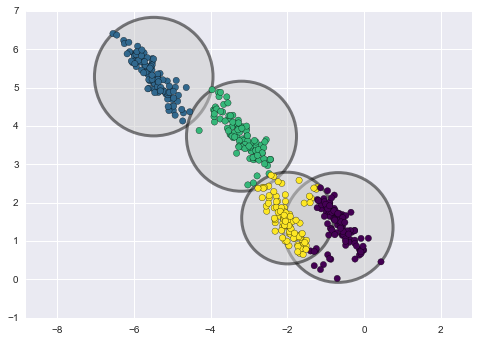
By eye, we recognize that these transformed clusters are noncircular, and thus circular clusters would be a poor fit. Nevertheless, k-means is not flexible enough to account for this, and tries to force-fit the data into four circular clusters. This results in a mixing of cluster assignments where the resulting circles overlap: see especially the bottom right of this plot. One might imagine addressing this particular situation by preprocessing the data with PCA (see “In Depth: Principal Component Analysis”), but in practice there is no guarantee that such a global operation will circularize the individual data.
These two disadvantages of k-means—its lack of flexibility in cluster shape and lack of probabilistic cluster assignment—mean that for many datasets (especially low-dimensional datasets) it may not perform as well as you might hope.
You might imagine addressing these weaknesses by generalizing the k-means model: for example, you could measure uncertainty in cluster assignment by comparing the distances of each point to all cluster centers, rather than focusing on just the closest. You might also imagine allowing the cluster boundaries to be ellipses rather than circles, so as to account for noncircular clusters. It turns out these are two essential components of a different type of clustering model, Gaussian mixture models.
A Gaussian mixture model (GMM) attempts to find a mixture of multidimensional Gaussian probability distributions that best model any input dataset. In the simplest case, GMMs can be used for finding clusters in the same manner as k-means (Figure 5-127):
In[7]:fromsklearn.mixtureimportGMMgmm=GMM(n_components=4).fit(X)labels=gmm.predict(X)plt.scatter(X[:,0],X[:,1],c=labels,s=40,cmap='viridis');
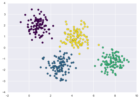
But because GMM contains a probabilistic model under the hood, it is
also possible to find probabilistic cluster assignments—in
Scikit-Learn we do this using the predict_proba method. This returns
a matrix of size [n_samples, n_clusters] that measures the
probability that any point belongs to the given cluster:
In[8]:probs=gmm.predict_proba(X)(probs[:5].round(3))
[[ 0. 0. 0.475 0.525] [ 0. 1. 0. 0. ] [ 0. 1. 0. 0. ] [ 0. 0. 0. 1. ] [ 0. 1. 0. 0. ]]
We can visualize this uncertainty by, for example, making the size of each point proportional to the certainty of its prediction; looking at Figure 5-128, we can see that it is precisely the points at the boundaries between clusters that reflect this uncertainty of cluster assignment:
In[9]:size=50*probs.max(1)**2# square emphasizes differencesplt.scatter(X[:,0],X[:,1],c=labels,cmap='viridis',s=size);

Under the hood, a Gaussian mixture model is very similar to k-means: it uses an expectation–maximization approach that qualitatively does the following:
Choose starting guesses for the location and shape
Repeat until converged:
E-step: for each point, find weights encoding the probability of membership in each cluster
M-step: for each cluster, update its location, normalization, and shape based on all data points, making use of the weights
The result of this is that each cluster is associated not with a hard-edged sphere, but with a smooth Gaussian model. Just as in the k-means expectation–maximization approach, this algorithm can sometimes miss the globally optimal solution, and thus in practice multiple random initializations are used.
Let’s create a function that will help us visualize the locations and
shapes of the GMM clusters by drawing ellipses based on the gmm output:
In[10]:frommatplotlib.patchesimportEllipsedefdraw_ellipse(position,covariance,ax=None,**kwargs):"""Draw an ellipse with a given position and covariance"""ax=axorplt.gca()# Convert covariance to principal axesifcovariance.shape==(2,2):U,s,Vt=np.linalg.svd(covariance)angle=np.degrees(np.arctan2(U[1,0],U[0,0]))width,height=2*np.sqrt(s)else:angle=0width,height=2*np.sqrt(covariance)# Draw the ellipsefornsiginrange(1,4):ax.add_patch(Ellipse(position,nsig*width,nsig*height,angle,**kwargs))defplot_gmm(gmm,X,label=True,ax=None):ax=axorplt.gca()labels=gmm.fit(X).predict(X)iflabel:ax.scatter(X[:,0],X[:,1],c=labels,s=40,cmap='viridis',zorder=2)else:ax.scatter(X[:,0],X[:,1],s=40,zorder=2)ax.axis('equal')w_factor=0.2/gmm.weights_.max()forpos,covar,winzip(gmm.means_,gmm.covars_,gmm.weights_):draw_ellipse(pos,covar,alpha=w*w_factor)
With this in place, we can take a look at what the four-component GMM gives us for our initial data (Figure 5-129):
In[11]:gmm=GMM(n_components=4,random_state=42)plot_gmm(gmm,X)
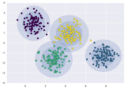
Similarly, we can use the GMM approach to fit our stretched dataset; allowing for a full covariance, the model will fit even very oblong, stretched-out clusters (Figure 5-130):
In[12]:gmm=GMM(n_components=4,covariance_type='full',random_state=42)plot_gmm(gmm,X_stretched)
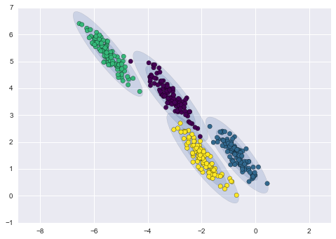
This makes clear that GMMs address the two main practical issues with k-means encountered before.
If you look at the details of the preceding fits, you will see that the
covariance_type option was set differently within each. This
hyperparameter controls the degrees of freedom in the shape of each
cluster; it is essential to set this carefully for any given problem.
The default is covariance_type="diag", which means that the size of
the cluster along each dimension can be set independently, with the
resulting ellipse constrained to align with the axes. A slightly simpler
and faster model is covariance_type="spherical", which constrains the
shape of the cluster such that all dimensions are equal. The resulting
clustering will have similar characteristics to that of k-means, though
it is not entirely equivalent. A more complicated and computationally
expensive model (especially as the number of dimensions grows) is to use
covariance_type="full", which allows each cluster to be modeled as an
ellipse with arbitrary orientation.
We can see a visual representation of these three choices for a single cluster within Figure 5-131:
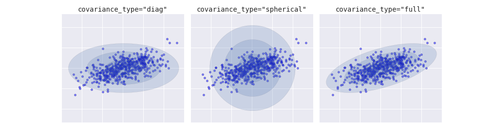
Though GMM is often categorized as a clustering algorithm, fundamentally it is an algorithm for density estimation. That is to say, the result of a GMM fit to some data is technically not a clustering model, but a generative probabilistic model describing the distribution of the data.
As an example, consider some data generated from Scikit-Learn’s
make_moons function (visualized in Figure 5-132), which we saw in “In Depth: k-Means Clustering”:
In[13]:fromsklearn.datasetsimportmake_moonsXmoon,ymoon=make_moons(200,noise=.05,random_state=0)plt.scatter(Xmoon[:,0],Xmoon[:,1]);
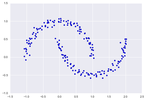
If we try to fit this to a two-component GMM viewed as a clustering model, the results are not particularly useful (Figure 5-133):
In[14]:gmm2=GMM(n_components=2,covariance_type='full',random_state=0)plot_gmm(gmm2,Xmoon)
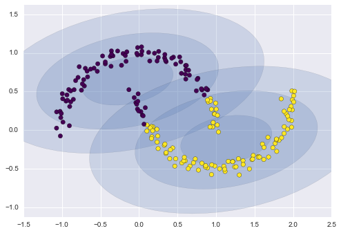
But if we instead use many more components and ignore the cluster labels, we find a fit that is much closer to the input data (Figure 5-134):
In[15]:gmm16=GMM(n_components=16,covariance_type='full',random_state=0)plot_gmm(gmm16,Xmoon,label=False)
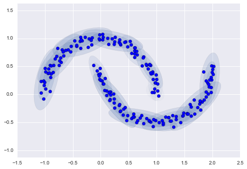
Here the mixture of 16 Gaussians serves not to find separated clusters of data, but rather to model the overall distribution of the input data. This is a generative model of the distribution, meaning that the GMM gives us the recipe to generate new random data distributed similarly to our input. For example, here are 400 new points drawn from this 16-component GMM fit to our original data (Figure 5-135):
In[16]:Xnew=gmm16.sample(400,random_state=42)plt.scatter(Xnew[:,0],Xnew[:,1]);
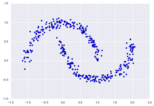
GMM is convenient as a flexible means of modeling an arbitrary multidimensional distribution of data.
The fact that GMM is a generative model gives us a natural means of determining the optimal number of components for a given dataset. A generative model is inherently a probability distribution for the dataset, and so we can simply evaluate the likelihood of the data under the model, using cross-validation to avoid overfitting. Another means of correcting for overfitting is to adjust the model likelihoods using some analytic criterion such as the Akaike information criterion (AIC) or the Bayesian information criterion (BIC). Scikit-Learn’s GMM estimator actually includes built-in methods that compute both of these, and so it is very easy to operate on this approach.
Let’s look at the AIC and BIC as a function as the number of GMM components for our moon dataset (Figure 5-136):
In[17]:n_components=np.arange(1,21)models=[GMM(n,covariance_type='full',random_state=0).fit(Xmoon)forninn_components]plt.plot(n_components,[m.bic(Xmoon)forminmodels],label='BIC')plt.plot(n_components,[m.aic(Xmoon)forminmodels],label='AIC')plt.legend(loc='best')plt.xlabel('n_components');
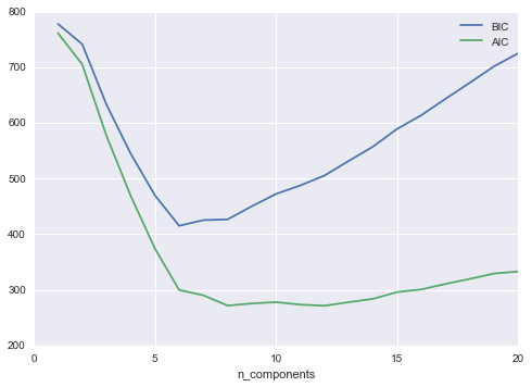
The optimal number of clusters is the value that minimizes the AIC or BIC, depending on which approximation we wish to use. The AIC tells us that our choice of 16 components was probably too many: around 8–12 components would have been a better choice. As is typical with this sort of problem, the BIC recommends a simpler model.
Notice the important point: this choice of number of components measures how well GMM works as a density estimator, not how well it works as a clustering algorithm. I’d encourage you to think of GMM primarily as a density estimator, and use it for clustering only when warranted within simple datasets.
We just saw a simple example of using GMM as a generative model of data in order to create new samples from the distribution defined by the input data. Here we will run with this idea and generate new handwritten digits from the standard digits corpus that we have used before.
To start with, let’s load the digits data using Scikit-Learn’s data tools:
In[18]:fromsklearn.datasetsimportload_digitsdigits=load_digits()digits.data.shape
Out[18]: (1797, 64)
Next let’s plot the first 100 of these to recall exactly what we’re looking at (Figure 5-137):
In[19]:defplot_digits(data):fig,ax=plt.subplots(10,10,figsize=(8,8),subplot_kw=dict(xticks=[],yticks=[]))fig.subplots_adjust(hspace=0.05,wspace=0.05)fori,axiinenumerate(ax.flat):im=axi.imshow(data[i].reshape(8,8),cmap='binary')im.set_clim(0,16)plot_digits(digits.data)
We have nearly 1,800 digits in 64 dimensions, and we can build a GMM on top of these to generate more. GMMs can have difficulty converging in such a high dimensional space, so we will start with an invertible dimensionality reduction algorithm on the data. Here we will use a straightforward PCA, asking it to preserve 99% of the variance in the projected data:
In[20]:fromsklearn.decompositionimportPCApca=PCA(0.99,whiten=True)data=pca.fit_transform(digits.data)data.shape
Out[20]: (1797, 41)
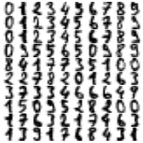
The result is 41 dimensions, a reduction of nearly 1/3 with almost no information loss. Given this projected data, let’s use the AIC to get a gauge for the number of GMM components we should use (Figure 5-138):
In[21]:n_components=np.arange(50,210,10)models=[GMM(n,covariance_type='full',random_state=0)forninn_components]aics=[model.fit(data).aic(data)formodelinmodels]plt.plot(n_components,aics);
It appears that around 110 components minimizes the AIC; we will use this model. Let’s quickly fit this to the data and confirm that it has converged:
In[22]:gmm=GMM(110,covariance_type='full',random_state=0)gmm.fit(data)(gmm.converged_)
True
Now we can draw samples of 100 new points within this 41-dimensional projected space, using the GMM as a generative model:
In[23]:data_new=gmm.sample(100,random_state=0)data_new.shape
Out[23]: (100, 41)
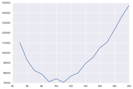
Finally, we can use the inverse transform of the PCA object to construct the new digits (Figure 5-139):
In[24]:digits_new=pca.inverse_transform(data_new)plot_digits(digits_new)
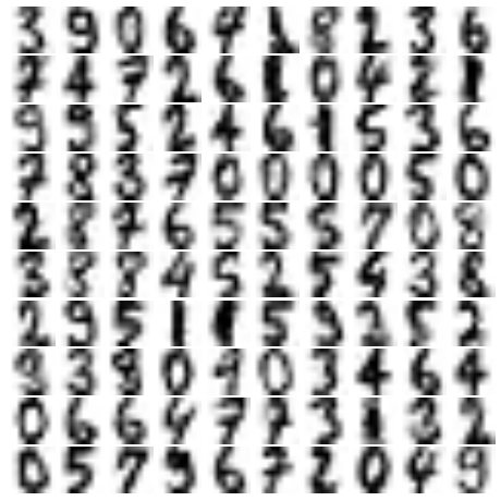
The results for the most part look like plausible digits from the dataset!
Consider what we’ve done here: given a sampling of handwritten digits, we have modeled the distribution of that data in such a way that we can generate brand new samples of digits from the data: these are “handwritten digits” that do not individually appear in the original dataset, but rather capture the general features of the input data as modeled by the mixture model. Such a generative model of digits can prove very useful as a component of a Bayesian generative classifier, as we shall see in the next section.
In the previous section we covered Gaussian mixture models (GMM), which
are a kind of hybrid between a clustering estimator and a density
estimator. Recall that a density estimator is an algorithm that takes a
 -dimensional dataset and produces an estimate of the
 -dimensional probability distribution which that data is
drawn from. The GMM algorithm accomplishes this by representing the
density as a weighted sum of Gaussian distributions. Kernel density
estimation (KDE) is in some senses an algorithm that takes the
mixture-of-Gaussians idea to its logical extreme: it uses a mixture
consisting of one Gaussian component per point, resulting in an
essentially nonparametric estimator of density. In this section, we
will explore the motivation and uses of KDE. We begin with the standard imports:
-dimensional probability distribution which that data is
drawn from. The GMM algorithm accomplishes this by representing the
density as a weighted sum of Gaussian distributions. Kernel density
estimation (KDE) is in some senses an algorithm that takes the
mixture-of-Gaussians idea to its logical extreme: it uses a mixture
consisting of one Gaussian component per point, resulting in an
essentially nonparametric estimator of density. In this section, we
will explore the motivation and uses of KDE. We begin with the standard imports:
In[1]:%matplotlibinlineimportmatplotlib.pyplotaspltimportseabornassns;sns.set()importnumpyasnp
As already discussed, a density estimator is an algorithm that seeks to model the probability distribution that generated a dataset. For one-dimensional data, you are probably already familiar with one simple density estimator: the histogram. A histogram divides the data into discrete bins, counts the number of points that fall in each bin, and then visualizes the results in an intuitive manner.
For example, let’s create some data that is drawn from two normal distributions:
In[2]:defmake_data(N,f=0.3,rseed=1):rand=np.random.RandomState(rseed)x=rand.randn(N)x[int(f*N):]+=5returnxx=make_data(1000)
We have previously seen that the standard count-based histogram can be
created with the plt.hist() function. By specifying the normed
parameter of the histogram, we end up with a normalized histogram where
the height of the bins does not reflect counts, but instead reflects
probability density (Figure 5-140):
In[3]:hist=plt.hist(x,bins=30,normed=True)
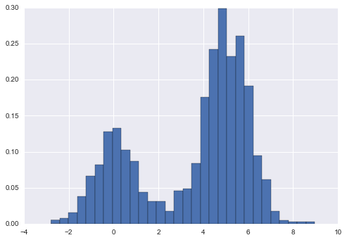
Notice that for equal binning, this normalization simply changes the scale on the y-axis, leaving the relative heights essentially the same as in a histogram built from counts. This normalization is chosen so that the total area under the histogram is equal to 1, as we can confirm by looking at the output of the histogram function:
In[4]:density,bins,patches=histwidths=bins[1:]-bins[:-1](density*widths).sum()
Out[4]: 1.0
One of the issues with using a histogram as a density estimator is that the choice of bin size and location can lead to representations that have qualitatively different features. For example, if we look at a version of this data with only 20 points, the choice of how to draw the bins can lead to an entirely different interpretation of the data! Consider this example (visualized in Figure 5-141):
In[5]:x=make_data(20)bins=np.linspace(-5,10,10)
In[6]:fig,ax=plt.subplots(1,2,figsize=(12,4),sharex=True,sharey=True,subplot_kw={'xlim':(-4,9),'ylim':(-0.02,0.3)})fig.subplots_adjust(wspace=0.05)fori,offsetinenumerate([0.0,0.6]):ax[i].hist(x,bins=bins+offset,normed=True)ax[i].plot(x,np.full_like(x,-0.01),'|k',markeredgewidth=1)
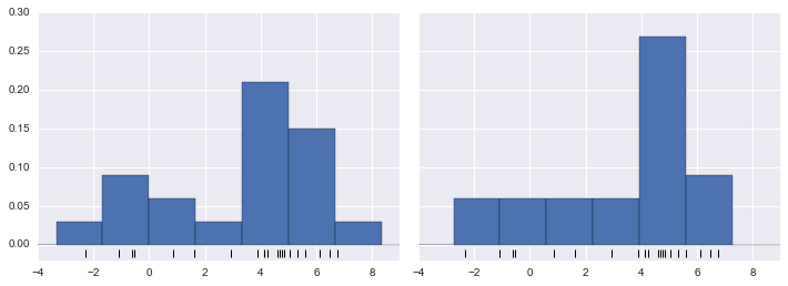
On the left, the histogram makes clear that this is a bimodal distribution. On the right, we see a unimodal distribution with a long tail. Without seeing the preceding code, you would probably not guess that these two histograms were built from the same data. With that in mind, how can you trust the intuition that histograms confer? And how might we improve on this?
Stepping back, we can think of a histogram as a stack of blocks, where we stack one block within each bin on top of each point in the dataset. Let’s view this directly (Figure 5-142):
In[7]:fig,ax=plt.subplots()bins=np.arange(-3,8)ax.plot(x,np.full_like(x,-0.1),'|k',markeredgewidth=1)forcount,edgeinzip(*np.histogram(x,bins)):foriinrange(count):ax.add_patch(plt.Rectangle((edge,i),1,1,alpha=0.5))ax.set_xlim(-4,8)ax.set_ylim(-0.2,8)
Out[7]: (-0.2, 8)
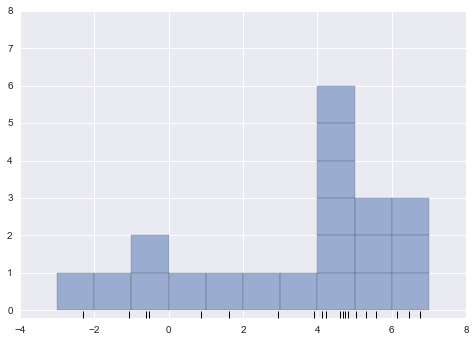
The problem with our two binnings stems from the fact that the height of the block stack often reflects not on the actual density of points nearby, but on coincidences of how the bins align with the data points. This misalignment between points and their blocks is a potential cause of the poor histogram results seen here. But what if, instead of stacking the blocks aligned with the bins, we were to stack the blocks aligned with the points they represent? If we do this, the blocks won’t be aligned, but we can add their contributions at each location along the x-axis to find the result. Let’s try this (Figure 5-143):
In[8]:x_d=np.linspace(-4,8,2000)density=sum((abs(xi-x_d)<0.5)forxiinx)plt.fill_between(x_d,density,alpha=0.5)plt.plot(x,np.full_like(x,-0.1),'|k',markeredgewidth=1)plt.axis([-4,8,-0.2,8]);
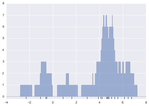
The result looks a bit messy, but is a much more robust reflection of the actual data characteristics than is the standard histogram. Still, the rough edges are not aesthetically pleasing, nor are they reflective of any true properties of the data. In order to smooth them out, we might decide to replace the blocks at each location with a smooth function, like a Gaussian. Let’s use a standard normal curve at each point instead of a block (Figure 5-144):
In[9]:fromscipy.statsimportnormx_d=np.linspace(-4,8,1000)density=sum(norm(xi).(x_d)forxiinx)plt.fill_between(x_d,density,alpha=0.5)plt.plot(x,np.full_like(x,-0.1),'|k',markeredgewidth=1)plt.axis([-4,8,-0.2,5]);
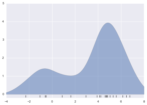
This smoothed-out plot, with a Gaussian distribution contributed at the location of each input point, gives a much more accurate idea of the shape of the data distribution, and one that has much less variance (i.e., changes much less in response to differences in sampling).
These last two plots are examples of kernel density estimation in one dimension: the first uses a so-called “tophat” kernel and the second uses a Gaussian kernel. We’ll now look at kernel density estimation in more detail.
The free parameters of kernel density estimation are the kernel, which specifies the shape of the distribution placed at each point, and the kernel bandwidth, which controls the size of the kernel at each point. In practice, there are many kernels you might use for a kernel density estimation: in particular, the Scikit-Learn KDE implementation supports one of six kernels, which you can read about in Scikit-Learn’s Density Estimation documentation.
While there are several versions of kernel density estimation
implemented in Python (notably in the SciPy and StatsModels packages), I
prefer to use Scikit-Learn’s version because of its efficiency and
flexibility. It is implemented in the sklearn.neighbors.KernelDensity
estimator, which handles KDE in multiple dimensions with one of six
kernels and one of a couple dozen distance metrics. Because KDE can be
fairly computationally intensive, the Scikit-Learn estimator uses a
tree-based algorithm under the hood and can trade off computation time
for accuracy using the atol (absolute tolerance) and rtol (relative
tolerance) parameters. We can determine the kernel bandwidth, which is a free parameter, using Scikit-Learn’s standard cross-validation tools,
as we will soon see.
Let’s first see a simple example of replicating the preceding plot using
the Scikit-Learn KernelDensity estimator (Figure 5-145):
In[10]:fromsklearn.neighborsimportKernelDensity# instantiate and fit the KDE modelkde=KernelDensity(bandwidth=1.0,kernel='gaussian')kde.fit(x[:,None])# score_samples returns the log of the probability densitylogprob=kde.score_samples(x_d[:,None])plt.fill_between(x_d,np.exp(logprob),alpha=0.5)plt.plot(x,np.full_like(x,-0.01),'|k',markeredgewidth=1)plt.ylim(-0.02,0.22)
Out[10]: (-0.02, 0.22)
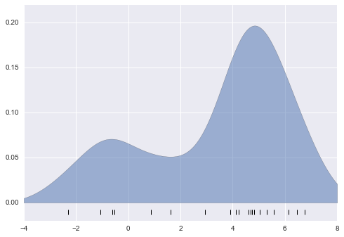
The result here is normalized such that the area under the curve is equal to 1.
The choice of bandwidth within KDE is extremely important to finding a suitable density estimate, and is the knob that controls the bias–variance trade-off in the estimate of density: too narrow a bandwidth leads to a high-variance estimate (i.e., overfitting), where the presence or absence of a single point makes a large difference. Too wide a bandwidth leads to a high-bias estimate (i.e., underfitting) where the structure in the data is washed out by the wide kernel.
There is a long history in statistics of methods to quickly estimate the best bandwidth based on rather stringent assumptions about the data: if you look up the KDE implementations in the SciPy and StatsModels packages, for example, you will see implementations based on some of these rules.
In machine learning contexts, we’ve seen that such hyperparameter tuning
often is done empirically via a cross-validation approach. With this in
mind, the KernelDensity estimator in Scikit-Learn is designed such
that it can be used directly within Scikit-Learn’s standard grid
search tools. Here we will use GridSearchCV to optimize the bandwidth
for the preceding dataset. Because we are looking at such a small dataset,
we will use leave-one-out cross-validation, which minimizes the
reduction in training set size for each cross-validation trial:
In[11]:fromsklearn.grid_searchimportGridSearchCVfromsklearn.cross_validationimportLeaveOneOutbandwidths=10**np.linspace(-1,1,100)grid=GridSearchCV(KernelDensity(kernel='gaussian'),{'bandwidth':bandwidths},cv=LeaveOneOut(len(x)))grid.fit(x[:,None]);
Now we can find the choice of bandwidth that maximizes the score (which in this case defaults to the log-likelihood):
In[12]:grid.best_params_
Out[12]: {'bandwidth': 1.1233240329780276}
The optimal bandwidth happens to be very close to what we used in the
example plot earlier, where the bandwidth was 1.0 (i.e., the default width
of scipy.stats.norm).
Perhaps the most common use of KDE is in graphically representing distributions of points. For example, in the Seaborn visualization library (discussed earlier in “Visualization with Seaborn”), KDE is built in and automatically used to help visualize points in one and two dimensions.
Here we will look at a slightly more sophisticated use of KDE for visualization of distributions. We will make use of some geographic data that can be loaded with Scikit-Learn: the geographic distributions of recorded observations of two South American mammals, Bradypus variegatus (the brown-throated sloth) and Microryzomys minutus (the forest small rice rat).
With Scikit-Learn, we can fetch this data as follows:
In[13]:fromsklearn.datasetsimportfetch_species_distributionsdata=fetch_species_distributions()# Get matrices/arrays of species IDs and locationslatlon=np.vstack([data.train['dd lat'],data.train['dd long']]).Tspecies=np.array([d.decode('ascii').startswith('micro')fordindata.train['species']],dtype='int')
With this data loaded, we can use the Basemap toolkit (mentioned previously in “Geographic Data with Basemap”) to plot the observed locations of these two species on the map of South America (Figure 5-146):
In[14]:frommpl_toolkits.basemapimportBasemapfromsklearn.datasets.species_distributionsimportconstruct_gridsxgrid,ygrid=construct_grids(data)# plot coastlines with Basemapm=Basemap(projection='cyl',resolution='c',llcrnrlat=ygrid.min(),urcrnrlat=ygrid.max(),llcrnrlon=xgrid.min(),urcrnrlon=xgrid.max())m.drawmapboundary(fill_color='#DDEEFF')m.fillcontinents(color='#FFEEDD')m.drawcoastlines(color='gray',zorder=2)m.drawcountries(color='gray',zorder=2)# plot locationsm.scatter(latlon[:,1],latlon[:,0],zorder=3,c=species,cmap='rainbow',latlon=True);
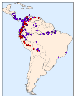
Unfortunately, this doesn’t give a very good idea of the density of the species, because points in the species range may overlap one another. You may not realize it by looking at this plot, but there are over 1,600 points shown here!
Let’s use kernel density estimation to show this distribution in a more
interpretable way: as a smooth indication of density on the map. Because
the coordinate system here lies on a spherical surface rather than a
flat plane, we will use the haversine distance metric, which will
correctly represent distances on a curved surface.
There is a bit of boilerplate code here (one of the disadvantages of the Basemap toolkit), but the meaning of each code block should be clear (Figure 5-147):
In[15]:# Set up the data grid for the contour plotX,Y=np.meshgrid(xgrid[::5],ygrid[::5][::-1])land_reference=data.coverages[6][::5,::5]land_mask=(land_reference>-9999).ravel()xy=np.vstack([Y.ravel(),X.ravel()]).Txy=np.radians(xy[land_mask])# Create two side-by-side plotsfig,ax=plt.subplots(1,2)fig.subplots_adjust(left=0.05,right=0.95,wspace=0.05)species_names=['Bradypus Variegatus','Microryzomys Minutus']cmaps=['Purples','Reds']fori,axiinenumerate(ax):axi.set_title(species_names[i])# plot coastlines with Basemapm=Basemap(projection='cyl',llcrnrlat=Y.min(),urcrnrlat=Y.max(),llcrnrlon=X.min(),urcrnrlon=X.max(),resolution='c',ax=axi)m.drawmapboundary(fill_color='#DDEEFF')m.drawcoastlines()m.drawcountries()# construct a spherical kernel density estimate of the distributionkde=KernelDensity(bandwidth=0.03,metric='haversine')kde.fit(np.radians(latlon[species==i]))# evaluate only on the land: -9999 indicates oceanZ=np.full(land_mask.shape[0],-9999.0)Z[land_mask]=np.exp(kde.score_samples(xy))Z=Z.reshape(X.shape)# plot contours of the densitylevels=np.linspace(0,Z.max(),25)axi.contourf(X,Y,Z,levels=levels,cmap=cmaps[i])
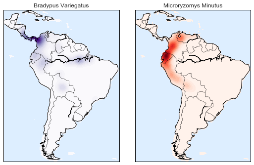
Compared to the simple scatter plot we initially used, this visualization paints a much clearer picture of the geographical distribution of observations of these two species.
This example looks at Bayesian generative classification with KDE, and demonstrates how to use the Scikit-Learn architecture to create a custom estimator.
In “In Depth: Naive Bayes Classification”, we took a look at naive Bayesian classification, in which we created a simple generative model for each class, and used these models to build a fast classifier. For naive Bayes, the generative model is a simple axis-aligned Gaussian. With a density estimation algorithm like KDE, we can remove the “naive” element and perform the same classification with a more sophisticated generative model for each class. It’s still Bayesian classification, but it’s no longer naive.
The general approach for generative classification is this:
Split the training data by label.
For each set, fit a KDE to obtain a generative model of the data.
This allows you for any observation  and label
 to compute a likelihood
  .
.
From the number of examples of each class in the training set,
compute the class prior,  .
.
For an unknown point  , the posterior probability for
each class is
, the posterior probability for
each class is 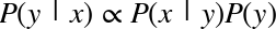 . The class
that maximizes this posterior is the label assigned to the point.
. The class
that maximizes this posterior is the label assigned to the point.
The algorithm is straightforward and intuitive to understand; the more difficult piece is couching it within the Scikit-Learn framework in order to make use of the grid search and cross-validation architecture.
This is the code that implements the algorithm within the Scikit-Learn framework; we will step through it following the code block:
In[16]:fromsklearn.baseimportBaseEstimator,ClassifierMixinclassKDEClassifier(BaseEstimator,ClassifierMixin):"""Bayesian generative classification based on KDEParameters----------bandwidth : floatthe kernel bandwidth within each classkernel : strthe kernel name, passed to KernelDensity"""def__init__(self,bandwidth=1.0,kernel='gaussian'):self.bandwidth=bandwidthself.kernel=kerneldeffit(self,X,y):self.classes_=np.sort(np.unique(y))training_sets=[X[y==yi]foryiinself.classes_]self.models_=[KernelDensity(bandwidth=self.bandwidth,kernel=self.kernel).fit(Xi)forXiintraining_sets]self.logpriors_=[np.log(Xi.shape[0]/X.shape[0])forXiintraining_sets]returnselfdefpredict_proba(self,X):logprobs=np.array([model.score_samples(X)formodelinself.models_]).Tresult=np.exp(logprobs+self.logpriors_)returnresult/result.sum(1,keepdims=True)defpredict(self,X):returnself.classes_[np.argmax(self.predict_proba(X),1)]
Let’s step through this code and discuss the essential features:
fromsklearn.baseimportBaseEstimator,ClassifierMixinclassKDEClassifier(BaseEstimator,ClassifierMixin):"""Bayesian generative classification based on KDEParameters----------bandwidth : floatthe kernel bandwidth within each classkernel : strthe kernel name, passed to KernelDensity"""
Each estimator in Scikit-Learn is a class, and it is most convenient for
this class to inherit from the BaseEstimator class as well as the
appropriate mixin, which provides standard functionality. For example,
among other things, here the BaseEstimator contains the logic
necessary to clone/copy an estimator for use in a cross-validation
procedure, and ClassifierMixin defines a default score() method used
by such routines. We also provide a docstring, which will be captured
by IPython’s help functionality (see
“Help and Documentation in IPython”).
Next comes the class initialization method:
def__init__(self,bandwidth=1.0,kernel='gaussian'):self.bandwidth=bandwidthself.kernel=kernel
This is the actual code executed when the object is instantiated
with KDEClassifier(). In Scikit-Learn, it is important that
initialization contains no operations other than assigning the passed
values by name to self. This is due to the logic contained in
BaseEstimator required for cloning and modifying estimators for cross-validation, grid search, and other functions. Similarly, all arguments
to __init__ should be explicit; that is, *args or **kwargs should be
avoided, as they will not be correctly handled within cross-validation
routines.
Next comes the fit() method, where we handle training data:
deffit(self,X,y):self.classes_=np.sort(np.unique(y))training_sets=[X[y==yi]foryiinself.classes_]self.models_=[KernelDensity(bandwidth=self.bandwidth,kernel=self.kernel).fit(Xi)forXiintraining_sets]self.logpriors_=[np.log(Xi.shape[0]/X.shape[0])forXiintraining_sets]returnself
Here we find the unique classes in the training data, train a
KernelDensity model for each class, and compute the class priors based
on the number of input samples. Finally, fit() should always return
self so that we can chain commands. For example:
label=model.fit(X,y).predict(X)
Notice that each persistent result of the fit is stored with a trailing
underscore (e.g., self.logpriors_). This is a convention used in
Scikit-Learn so that you can quickly scan the members of an estimator
(using IPython’s tab completion) and see exactly which members are
fit to training data.
Finally, we have the logic for predicting labels on new data:
defpredict_proba(self,X):logprobs=np.vstack([model.score_samples(X)formodelinself.models_]).Tresult=np.exp(logprobs+self.logpriors_)returnresult/result.sum(1,keepdims=True)defpredict(self,X):returnself.classes_[np.argmax(self.predict_proba(X),1)]
Because this is a probabilistic classifier, we first implement
predict_proba(), which returns an array of class probabilities of shape
[n_samples, n_classes]. Entry [i, j] of this array is the posterior
probability that sample i is a member of class j, computed by
multiplying the likelihood by the class prior and normalizing.
Finally, the predict() method uses these probabilities and simply
returns the class with the largest probability.
Let’s try this custom estimator on a problem we have seen before: the
classification of handwritten digits. Here we will load the digits, and
compute the cross-validation score for a range of candidate bandwidths
using the GridSearchCV meta-estimator (refer back to “Hyperparameters and Model Validation” for more information on this):
In[17]:fromsklearn.datasetsimportload_digitsfromsklearn.grid_searchimportGridSearchCVdigits=load_digits()bandwidths=10**np.linspace(0,2,100)grid=GridSearchCV(KDEClassifier(),{'bandwidth':bandwidths})grid.fit(digits.data,digits.target)scores=[val.mean_validation_scoreforvalingrid.grid_scores_]
Next we can plot the cross-validation score as a function of bandwidth (Figure 5-148):
In[18]:plt.semilogx(bandwidths,scores)plt.xlabel('bandwidth')plt.ylabel('accuracy')plt.title('KDE Model Performance')(grid.best_params_)('accuracy =',grid.best_score_)
{'bandwidth': 7.0548023107186433}
accuracy = 0.966611018364
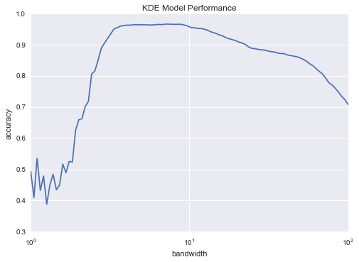
We see that this not-so-naive Bayesian classifier reaches a cross-validation accuracy of just over 96%; this is compared to around 80% for the naive Bayesian classification:
In[19]:fromsklearn.naive_bayesimportGaussianNBfromsklearn.cross_validationimportcross_val_scorecross_val_score(GaussianNB(),digits.data,digits.target).mean()
Out[19]: 0.81860038035501381
One benefit of such a generative classifier is interpretability of results: for each unknown sample, we not only get a probabilistic classification, but a full model of the distribution of points we are comparing it to! If desired, this offers an intuitive window into the reasons for a particular classification that algorithms like SVMs and random forests tend to obscure.
If you would like to take this further, there are some improvements that could be made to our KDE classifier model:
We could allow the bandwidth in each class to vary independently.
We could optimize these bandwidths not based on their prediction
score, but on the likelihood of the training data under the generative
model within each class (i.e., use the scores from KernelDensity itself
rather than the global prediction accuracy).
Finally, if you want some practice building your own estimator, you might tackle building a similar Bayesian classifier using Gaussian mixture models instead of KDE.
This chapter has explored a number of the central concepts and
algorithms of machine learning. But moving from these concepts to
real-world application can be a challenge. Real-world datasets are noisy
and heterogeneous, may have missing features, and may include data in a form
that is difficult to map to a clean [n_samples, n_features] matrix.
Before applying any of the methods discussed here, you must first
extract these features from your data; there is no formula for how to do
this that applies across all domains, and thus this is where you as a
data scientist must exercise your own intuition and expertise.
One interesting and compelling application of machine learning is to images, and we have already seen a few examples of this where pixel-level features are used for classification. In the real world, data is rarely so uniform and simple pixels will not be suitable, a fact that has led to a large literature on feature extraction methods for image data (see “Feature Engineering”).
In this section, we will take a look at one such feature extraction technique, the Histogram of Oriented Gradients (HOG), which transforms image pixels into a vector representation that is sensitive to broadly informative image features regardless of confounding factors like illumination. We will use these features to develop a simple face detection pipeline, using machine learning algorithms and concepts we’ve seen throughout this chapter. We begin with the standard imports:
In[1]:%matplotlibinlineimportmatplotlib.pyplotaspltimportseabornassns;sns.set()importnumpyasnp
The Histogram of Gradients is a straightforward feature extraction procedure that was developed in the context of identifying pedestrians within images. HOG involves the following steps:
Optionally prenormalize images. This leads to features that resist dependence on variations in illumination.
Convolve the image with two filters that are sensitive to horizontal and vertical brightness gradients. These capture edge, contour, and texture information.
Subdivide the image into cells of a predetermined size, and compute a histogram of the gradient orientations within each cell.
Normalize the histograms in each cell by comparing to the block of neighboring cells. This further suppresses the effect of illumination across the image.
Construct a one-dimensional feature vector from the information in each cell.
A fast HOG extractor is built into the Scikit-Image project, and we can try it out relatively quickly and visualize the oriented gradients within each cell (Figure 5-149):
In[2]:fromskimageimportdata,color,featureimportskimage.dataimage=color.rgb2gray(data.chelsea())hog_vec,hog_vis=feature.hog(image,visualise=True)fig,ax=plt.subplots(1,2,figsize=(12,6),subplot_kw=dict(xticks=[],yticks=[]))ax[0].imshow(image,cmap='gray')ax[0].set_title('input image')ax[1].imshow(hog_vis)ax[1].set_title('visualization of HOG features');
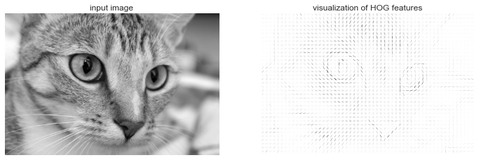
Using these HOG features, we can build up a simple facial detection algorithm with any Scikit-Learn estimator; here we will use a linear support vector machine (refer back to “In-Depth: Support Vector Machines” if you need a refresher on this). The steps are as follows:
Obtain a set of image thumbnails of faces to constitute “positive” training samples.
Obtain a set of image thumbnails of nonfaces to constitute “negative” training samples.
Extract HOG features from these training samples.
Train a linear SVM classifier on these samples.
For an “unknown” image, pass a sliding window across the image, using the model to evaluate whether that window contains a face or not.
If detections overlap, combine them into a single window.
Let’s go through these steps and try it out:
Obtain a set of positive training samples.
Let’s start by finding some positive training samples that show a variety of faces. We have one easy set of data to work with—the Labeled Faces in the Wild dataset, which can be downloaded by Scikit-Learn:
In[3]:fromsklearn.datasetsimportfetch_lfw_peoplefaces=fetch_lfw_people()positive_patches=faces.imagespositive_patches.shape
Out[3]: (13233, 62, 47)
This gives us a sample of 13,000 face images to use for training.
Obtain a set of negative training samples.
Next we need a set of similarly sized thumbnails that do not have a
face in them. One way to do this is to take any corpus of input images,
and extract thumbnails from them at a variety of scales. Here we can use
some of the images shipped with Scikit-Image, along with Scikit-Learn’s
PatchExtractor:
In[4]:fromskimageimportdata,transformimgs_to_use=['camera','text','coins','moon','page','clock','immunohistochemistry','chelsea','coffee','hubble_deep_field']images=[color.rgb2gray(getattr(data,name)())fornameinimgs_to_use]
In[5]:fromsklearn.feature_extraction.imageimportPatchExtractordefextract_patches(img,N,scale=1.0,patch_size=positive_patches[0].shape):extracted_patch_size=\tuple((scale*np.array(patch_size)).astype(int))extractor=PatchExtractor(patch_size=extracted_patch_size,max_patches=N,random_state=0)patches=extractor.transform(img[np.newaxis])ifscale!=1:patches=np.array([transform.resize(patch,patch_size)forpatchinpatches])returnpatchesnegative_patches=np.vstack([extract_patches(im,1000,scale)foriminimagesforscalein[0.5,1.0,2.0]])negative_patches.shape
Out[5]: (30000, 62, 47)
We now have 30,000 suitable image patches that do not contain faces. Let’s take a look at a few of them to get an idea of what they look like (Figure 5-150):
In[6]:fig,ax=plt.subplots(6,10)fori,axiinenumerate(ax.flat):axi.imshow(negative_patches[500*i],cmap='gray')axi.axis('off')
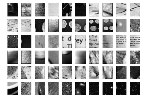
Our hope is that these would sufficiently cover the space of “nonfaces” that our algorithm is likely to see.
Combine sets and extract HOG features.
Now that we have these positive samples and negative samples, we can combine them and compute HOG features. This step takes a little while, because the HOG features involve a nontrivial computation for each image:
In[7]:fromitertoolsimportchainX_train=np.array([feature.hog(im)foriminchain(positive_patches,negative_patches)])y_train=np.zeros(X_train.shape[0])y_train[:positive_patches.shape[0]]=1
In[8]:X_train.shape
Out[8]: (43233, 1215)
We are left with 43,000 training samples in 1,215 dimensions, and we now have our data in a form that we can feed into Scikit-Learn!
Train a support vector machine.
Next we use the tools we have been exploring in this chapter to create a
classifier of thumbnail patches. For such a high-dimensional binary
classification task, a linear support vector machine is a good choice.
We will use Scikit-Learn’s LinearSVC, because in comparison to SVC
it often has better scaling for large number of samples.
First, though, let’s use a simple Gaussian naive Bayes to get a quick baseline:
In[9]:fromsklearn.naive_bayesimportGaussianNBfromsklearn.cross_validationimportcross_val_scorecross_val_score(GaussianNB(),X_train,y_train)
Out[9]: array([ 0.9408785 , 0.8752342 , 0.93976823])
We see that on our training data, even a simple naive Bayes algorithm gets us upward of 90% accuracy. Let’s try the support vector machine, with a grid search over a few choices of the C parameter:
In[10]:fromsklearn.svmimportLinearSVCfromsklearn.grid_searchimportGridSearchCVgrid=GridSearchCV(LinearSVC(),{'C':[1.0,2.0,4.0,8.0]})grid.fit(X_train,y_train)grid.best_score_
Out[10]: 0.98667684407744083
In[11]:grid.best_params_
Out[11]: {'C': 4.0}
Let’s take the best estimator and retrain it on the full dataset:
In[12]:model=grid.best_estimator_model.fit(X_train,y_train)
Out[12]: LinearSVC(C=4.0, class_weight=None, dual=True,
fit_intercept=True, intercept_scaling=1,
loss='squared_hinge', max_iter=1000,
multi_class='ovr', penalty='l2',
random_state=None, tol=0.0001, verbose=0)
Find faces in a new image.
Now that we have this model in place, let’s grab a new image and see how the model does. We will use one portion of the astronaut image for simplicity (see discussion of this in “Caveats and Improvements”), and run a sliding window over it and evaluate each patch (Figure 5-151):
In[13]:test_image=skimage.data.astronaut()test_image=skimage.color.rgb2gray(test_image)test_image=skimage.transform.rescale(test_image,0.5)test_image=test_image[:160,40:180]plt.imshow(test_image,cmap='gray')plt.axis('off');

Next, let’s create a window that iterates over patches of this image, and compute HOG features for each patch:
In[14]:defsliding_window(img,patch_size=positive_patches[0].shape,istep=2,jstep=2,scale=1.0):Ni,Nj=(int(scale*s)forsinpatch_size)foriinrange(0,img.shape[0]-Ni,istep):forjinrange(0,img.shape[1]-Ni,jstep):patch=img[i:i+Ni,j:j+Nj]ifscale!=1:patch=transform.resize(patch,patch_size)yield(i,j),patchindices,patches=zip(*sliding_window(test_image))patches_hog=np.array([feature.hog(patch)forpatchinpatches])patches_hog.shape
Out[14]: (1911, 1215)
Finally, we can take these HOG-featured patches and use our model to evaluate whether each patch contains a face:
In[15]:labels=model.predict(patches_hog)labels.sum()
Out[15]: 33.0
We see that out of nearly 2,000 patches, we have found 30 detections. Let’s use the information we have about these patches to show where they lie on our test image, drawing them as rectangles (Figure 5-152):
In[16]:fig,ax=plt.subplots()ax.imshow(test_image,cmap='gray')ax.axis('off')Ni,Nj=positive_patches[0].shapeindices=np.array(indices)fori,jinindices[labels==1]:ax.add_patch(plt.Rectangle((j,i),Nj,Ni,edgecolor='red',alpha=0.3,lw=2,facecolor='none'))
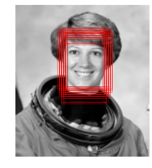
All of the detected patches overlap and found the face in the image! Not bad for a few lines of Python.
If you dig a bit deeper into the preceding code and examples, you’ll see that we still have a bit of work before we can claim a production-ready face detector. There are several issues with what we’ve done, and several improvements that could be made. In particular:
The central issue is that there are many face-like textures that are not in the training set, and so our current model is very prone to false positives. You can see this if you try out the preceding algorithm on the full astronaut image: the current model leads to many false detections in other regions of the image.
We might imagine addressing this by adding a wider variety of images to the negative training set, and this would probably yield some improvement. Another way to address this is to use a more directed approach, such as hard negative mining. In hard negative mining, we take a new set of images that our classifier has not seen, find all the patches representing false positives, and explicitly add them as negative instances in the training set before retraining the classifier.
As currently written, our algorithm will miss faces that are not
approximately 62×47 pixels. We can straightforwardly address this by
using sliding windows of a variety of sizes, and resizing each patch
using skimage.transform.resize before feeding it into the model.
In fact, the sliding_window() utility used here is already built with
this in mind.
For a production-ready pipeline, we would prefer not to have 30 detections of the same face, but to somehow reduce overlapping groups of detections down to a single detection. This could be done via an unsupervised clustering approach (MeanShift Clustering is one good candidate for this), or via a procedural approach such as nonmaximum suppression, an algorithm common in machine vision.
Once we address these issues, it would also be nice to create a more streamlined pipeline for ingesting training images and predicting sliding-window outputs. This is where Python as a data science tool really shines: with a bit of work, we could take our prototype code and package it with a well-designed object-oriented API that gives the user the ability to use this easily. I will leave this as a proverbial “exercise for the reader.”
Finally, I should add that HOG and other procedural feature extraction methods for images are no longer state-of-the-art techniques. Instead, many modern object detection pipelines use variants of deep neural networks. One way to think of neural networks is that they are an estimator that determines optimal feature extraction strategies from the data, rather than relying on the intuition of the user. An intro to these deep neural net methods is conceptually (and computationally!) beyond the scope of this section, although open tools like Google’s TensorFlow have recently made deep learning approaches much more accessible than they once were. As of the writing of this book, deep learning in Python is still relatively young, and so I can’t yet point to any definitive resource. That said, the list of references in the following section should provide a useful place to start.
This chapter has been a quick tour of machine learning in Python, primarily using the tools within the Scikit-Learn library. As long as the chapter is, it is still too short to cover many interesting and important algorithms, approaches, and discussions. Here I want to suggest some resources for those who would like to learn more about machine learning.
To learn more about machine learning in Python, I’d suggest some of the following resources:
The Scikit-Learn website has an impressive breadth of documentation and examples covering some of the models discussed here, and much, much more. If you want a brief survey of the most important and often used machine learning algorithms, this website is a good place to start.
Scikit-Learn and other machine learning topics are perennial favorites in the tutorial tracks of many Python-focused conference series, in particular the PyCon, SciPy, and PyData conferences. You can find the most recent ones via a simple web search.
Written by Andreas C. Mueller and Sarah Guido, this book includes a fuller treatment of the topics in this chapter. If you’re interested in reviewing the fundamentals of machine learning and pushing the Scikit-Learn toolkit to its limits, this is a great resource, written by one of the most prolific developers on the Scikit-Learn team.
Sebastian Raschka’s book focuses less on Scikit-Learn itself, and more on the breadth of machine learning tools available in Python. In particular, there is some very useful discussion on how to scale Python-based machine learning approaches to large and complex datasets.
Of course, machine learning is much broader than just the Python world. There are many good resources to take your knowledge further, and here I highlight a few that I have found useful:
Taught by Andrew Ng (Coursera), this is a very clearly taught, free online course covering the basics of machine learning from an algorithmic perspective. It assumes undergraduate-level understanding of mathematics and programming, and steps through detailed considerations of some of the most important machine learning algorithms. Homework assignments, which are algorithmically graded, have you actually implement some of these models yourself.
Written by Christopher Bishop, this classic technical text covers the concepts of machine learning discussed in this chapter in detail. If you plan to go further in this subject, you should have this book on your shelf.
Written by Kevin Murphy, this is an excellent graduate-level text that explores nearly all important machine learning algorithms from a ground-up, unified probabilistic perspective.
These resources are more technical than the material presented in this book, but to really understand the fundamentals of these methods requires a deep dive into the mathematics behind them. If you’re up for the challenge and ready to bring your data science to the next level, don’t hesitate to dive in!
The animal on the cover of Python Data Science Handbook is a Mexican beaded lizard (Heloderma horridum), a reptile found in Mexico and parts of Guatemala. It and the Gila monster (a close relative) are the only venomous lizards in the world. This animal primarily feeds on eggs, however, so the venom is used as a defense mechanism. When it feels threatened, the lizard will bite—and because it cannot release a large quantity of venom at once, it firmly clamps its jaws and uses a chewing motion to move the toxin deeper into the wound. This bite and the aftereffects of the venom are extremely painful, though rarely fatal to humans.
The Greek word heloderma translates to “studded skin,” referring to the distinctive beaded texture of the reptile’s skin. These bumps are osteoderms, which each contain a small piece of bone and serve as protective armor. The Mexican beaded lizard is black with yellow patches and bands. It has a broad head and a thick tail that stores fat to help the animal survive during the hot summer months when it is inactive. On average, these lizards are 22–36 inches long, and weigh around 1.8 pounds.
As with most snakes and lizards, the tongue of the Mexican beaded lizard is its primary sensory organ. It will flick it out repeatedly to gather scent particles from the environment and detect prey (or, during mating season, a potential partner). When the forked tongue is retracted into the mouth, it touches the Jacobson’s organ, a patch of sensory cells that identify various chemicals and pheromones.
The beaded lizard’s venom contains enzymes that have been synthesized to help treat diabetes, and further pharmacological research is in progress. It is endangered by loss of habitat, poaching for the pet trade, and being killed by locals who are simply afraid of it. This animal is protected by legislation in both countries where it lives.
Many of the animals on O’Reilly covers are endangered; all of them are important to the world. To learn more about how you can help, go to animals.oreilly.com.
The cover image is from Wood’s Animate Creation. The cover fonts are URW Typewriter and Guardian Sans. The text font is Adobe Minion Pro; the heading font is Adobe Myriad Condensed; and the code font is Dalton Maag’s Ubuntu Mono.
Essential Tools for Working with Data
Copyright © 2017 Jake VanderPlas. All rights reserved.
Printed in the United States of America.
Published by O’Reilly Media, Inc., 1005 Gravenstein Highway North, Sebastopol, CA 95472.
O’Reilly books may be purchased for educational, business, or sales promotional use. Online editions are also available for most titles (http://oreilly.com/safari). For more information, contact our corporate/institutional sales department: 800-998-9938 or corporate@oreilly.com.
See http://oreilly.com/catalog/errata.csp?isbn=9781491912058 for release details.
The O’Reilly logo is a registered trademark of O’Reilly Media, Inc. Python Data Science Handbook, the cover image, and related trade dress are trademarks of O’Reilly Media, Inc.
While the publisher and the author have used good faith efforts to ensure that the information and instructions contained in this work are accurate, the publisher and the author disclaim all responsibility for errors or omissions, including without limitation responsibility for damages resulting from the use of or reliance on this work. Use of the information and instructions contained in this work is at your own risk. If any code samples or other technology this work contains or describes is subject to open source licenses or the intellectual property rights of others, it is your responsibility to ensure that your use thereof complies with such licenses and/or rights.
978-1-491-91205-8
[LSI]
This is a book about doing data science with Python, which immediately begs the question: what is data science? It’s a surprisingly hard definition to nail down, especially given how ubiquitous the term has become. Vocal critics have variously dismissed the term as a superfluous label (after all, what science doesn’t involve data?) or a simple buzzword that only exists to salt résumés and catch the eye of overzealous tech recruiters.
In my mind, these critiques miss something important. Data science, despite its hype-laden veneer, is perhaps the best label we have for the cross-disciplinary set of skills that are becoming increasingly important in many applications across industry and academia. This cross-disciplinary piece is key: in my mind, the best existing definition of data science is illustrated by Drew Conway’s Data Science Venn Diagram, first published on his blog in September 2010 (see Figure P-1).
While some of the intersection labels are a bit tongue-in-cheek, this diagram captures the essence of what I think people mean when they say “data science”: it is fundamentally an interdisciplinary subject. Data science comprises three distinct and overlapping areas: the skills of a statistician who knows how to model and summarize datasets (which are growing ever larger); the skills of a computer scientist who can design and use algorithms to efficiently store, process, and visualize this data; and the domain expertise—what we might think of as “classical” training in a subject—necessary both to formulate the right questions and to put their answers in context.
With this in mind, I would encourage you to think of data science not as a new domain of knowledge to learn, but as a new set of skills that you can apply within your current area of expertise. Whether you are reporting election results, forecasting stock returns, optimizing online ad clicks, identifying microorganisms in microscope photos, seeking new classes of astronomical objects, or working with data in any other field, the goal of this book is to give you the ability to ask and answer new questions about your chosen subject area.
In my teaching both at the University of Washington and at various tech-focused conferences and meetups, one of the most common questions I have heard is this: “how should I learn Python?” The people asking are generally technically minded students, developers, or researchers, often with an already strong background in writing code and using computational and numerical tools. Most of these folks don’t want to learn Python per se, but want to learn the language with the aim of using it as a tool for data-intensive and computational science. While a large patchwork of videos, blog posts, and tutorials for this audience is available online, I’ve long been frustrated by the lack of a single good answer to this question; that is what inspired this book.
The book is not meant to be an introduction to Python or to programming in general; I assume the reader has familiarity with the Python language, including defining functions, assigning variables, calling methods of objects, controlling the flow of a program, and other basic tasks. Instead, it is meant to help Python users learn to use Python’s data science stack—libraries such as IPython, NumPy, Pandas, Matplotlib, Scikit-Learn, and related tools—to effectively store, manipulate, and gain insight from data.
Python has emerged over the last couple decades as a first-class tool for scientific computing tasks, including the analysis and visualization of large datasets. This may have come as a surprise to early proponents of the Python language: the language itself was not specifically designed with data analysis or scientific computing in mind. The usefulness of Python for data science stems primarily from the large and active ecosystem of third-party packages: NumPy for manipulation of homogeneous array-based data, Pandas for manipulation of heterogeneous and labeled data, SciPy for common scientific computing tasks, Matplotlib for publication-quality visualizations, IPython for interactive execution and sharing of code, Scikit-Learn for machine learning, and many more tools that will be mentioned in the following pages.
If you are looking for a guide to the Python language itself, I would suggest the sister project to this book, A Whirlwind Tour of the Python Language. This short report provides a tour of the essential features of the Python language, aimed at data scientists who already are familiar with one or more other programming languages.
This book uses the syntax of Python 3, which contains language enhancements that are not compatible with the 2.x series of Python. Though Python 3.0 was first released in 2008, adoption has been relatively slow, particularly in the scientific and web development communities. This is primarily because it took some time for many of the essential third-party packages and toolkits to be made compatible with the new language internals. Since early 2014, however, stable releases of the most important tools in the data science ecosystem have been fully compatible with both Python 2 and 3, and so this book will use the newer Python 3 syntax. However, the vast majority of code snippets in this book will also work without modification in Python 2: in cases where a Py2-incompatible syntax is used, I will make every effort to note it explicitly.
Each chapter of this book focuses on a particular package or tool that contributes a fundamental piece of the Python data science story.
These packages provide the computational environment in which many Python-using data scientists work.
This library provides the ndarray object for efficient storage and manipulation of dense data arrays in Python.
This library provides the DataFrame object for efficient storage
and manipulation of labeled/columnar data in Python.
This library provides capabilities for a flexible range of data visualizations in Python.
This library provides efficient and clean Python implementations of the most important and established machine learning algorithms.
The PyData world is certainly much larger than these five packages, and is growing every day. With this in mind, I make every attempt through these pages to provide references to other interesting efforts, projects, and packages that are pushing the boundaries of what can be done in Python. Nevertheless, these five are currently fundamental to much of the work being done in the Python data science space, and I expect they will remain important even as the ecosystem continues growing around them.
Supplemental material (code examples, figures, etc.) is available for download at https://github.com/jakevdp/PythonDataScienceHandbook. This book is here to help you get your job done. In general, if example code is offered with this book, you may use it in your programs and documentation. You do not need to contact us for permission unless you’re reproducing a significant portion of the code. For example, writing a program that uses several chunks of code from this book does not require permission. Selling or distributing a CD-ROM of examples from O’Reilly books does require permission. Answering a question by citing this book and quoting example code does not require permission. Incorporating a significant amount of example code from this book into your product’s documentation does require permission.
We appreciate, but do not require, attribution. An attribution usually includes the title, author, publisher, and ISBN. For example, “Python Data Science Handbook by Jake VanderPlas (O’Reilly). Copyright 2017 Jake VanderPlas, 978-1-491-91205-8.”
If you feel your use of code examples falls outside fair use or the permission given above, feel free to contact us at permissions@oreilly.com.
Installing Python and the suite of libraries that enable scientific computing is straightforward. This section will outline some of the considerations to keep in mind when setting up your computer.
Though there are various ways to install Python, the one I would suggest for use in data science is the Anaconda distribution, which works similarly whether you use Windows, Linux, or Mac OS X. The Anaconda distribution comes in two flavors:
Miniconda gives you the Python interpreter itself, along with a command-line tool called conda that operates as a cross-platform package manager geared toward Python packages, similar in spirit to the apt or yum tools that Linux users might be familiar with.
Anaconda includes both Python and conda, and additionally bundles a suite of other preinstalled packages geared toward scientific computing. Because of the size of this bundle, expect the installation to consume several gigabytes of disk space.
Any of the packages included with Anaconda can also be installed manually on top of Miniconda; for this reason I suggest starting with Miniconda.
To get started, download and install the Miniconda package (make sure to choose a version with Python 3), and then install the core packages used in this book:
[~]$ conda install numpy pandas scikit-learn matplotlib seaborn ipython-notebook
Throughout the text, we will also make use of other, more specialized tools
in Python’s scientific ecosystem; installation is usually as easy as
typing conda install packagename. For more information on conda,
including information about creating and using conda environments (which
I would highly recommend), refer to
conda’s online documentation.
The following typographical conventions are used in this book:
Indicates new terms, URLs, email addresses, filenames, and file extensions.
Constant widthUsed for program listings, as well as within paragraphs to refer to program elements such as variable or function names, databases, data types, environment variables, statements, and keywords.
Constant width boldShows commands or other text that should be typed literally by the user.
Constant width italicShows text that should be replaced with user-supplied values or by values determined by context.
Safari (formerly Safari Books Online) is a membership-based training and reference platform for enterprise, government, educators, and individuals.
Members have access to thousands of books, training videos, Learning Paths, interactive tutorials, and curated playlists from over 250 publishers, including O’Reilly Media, Harvard Business Review, Prentice Hall Professional, Addison-Wesley Professional, Microsoft Press, Sams, Que, Peachpit Press, Adobe, Focal Press, Cisco Press, John Wiley & Sons, Syngress, Morgan Kaufmann, IBM Redbooks, Packt, Adobe Press, FT Press, Apress, Manning, New Riders, McGraw-Hill, Jones & Bartlett, and Course Technology, among others.
For more information, please visit http://oreilly.com/safari.
Please address comments and questions concerning this book to the publisher:
We have a web page for this book, where we list errata, examples, and any additional information. You can access this page at http://bit.ly/python-data-sci-handbook.
To comment or ask technical questions about this book, send email to bookquestions@oreilly.com.
For more information about our books, courses, conferences, and news, see our website at http://www.oreilly.com.
Find us on Facebook: http://facebook.com/oreilly
Follow us on Twitter: http://twitter.com/oreillymedia
Watch us on YouTube: http://www.youtube.com/oreillymedia
There are many options for development environments for Python, and I’m often asked which one I use in my own work. My answer sometimes surprises people: my preferred environment is IPython plus a text editor (in my case, Emacs or Atom depending on my mood). IPython (short for Interactive Python) was started in 2001 by Fernando Perez as an enhanced Python interpreter, and has since grown into a project aiming to provide, in Perez’s words, “Tools for the entire lifecycle of research computing.” If Python is the engine of our data science task, you might think of IPython as the interactive control panel.
As well as being a useful interactive interface to Python, IPython also provides a number of useful syntactic additions to the language; we’ll cover the most useful of these additions here. In addition, IPython is closely tied with the Jupyter project, which provides a browser-based notebook that is useful for development, collaboration, sharing, and even publication of data science results. The IPython notebook is actually a special case of the broader Jupyter notebook structure, which encompasses notebooks for Julia, R, and other programming languages. As an example of the usefulness of the notebook format, look no further than the page you are reading: the entire manuscript for this book was composed as a set of IPython notebooks.
IPython is about using Python effectively for interactive scientific and data-intensive computing. This chapter will start by stepping through some of the IPython features that are useful to the practice of data science, focusing especially on the syntax it offers beyond the standard features of Python. Next, we will go into a bit more depth on some of the more useful “magic commands” that can speed up common tasks in creating and using data science code. Finally, we will touch on some of the features of the notebook that make it useful in understanding data and sharing results.
There are two primary means of using IPython that we’ll discuss in this chapter: the IPython shell and the IPython notebook. The bulk of the material in this chapter is relevant to both, and the examples will switch between them depending on what is most convenient. In the few sections that are relevant to just one or the other, I will explicitly state that fact. Before we start, some words on how to launch the IPython shell and IPython notebook.
This chapter, like most of this book, is not designed to be absorbed
passively. I recommend that as you read through it, you follow along and
experiment with the tools and syntax we cover: the muscle-memory you
build through doing this will be far more useful than the simple act of
reading about it. Start by launching the IPython interpreter by typing
ipython on the command line; alternatively, if you’ve installed a
distribution like Anaconda or EPD, there may be a launcher specific to
your system (we’ll discuss this more fully in “Help and Documentation in IPython”).
Once you do this, you should see a prompt like the following:
IPython 4.0.1 -- An enhanced Interactive Python. ? -> Introduction and overview of IPython's features. %quickref -> Quick reference. help -> Python's own help system. object? -> Details about 'object', use 'object??' for extra details. In [1]:
With that, you’re ready to follow along.
The Jupyter notebook is a browser-based graphical interface to the IPython shell, and builds on it a rich set of dynamic display capabilities. As well as executing Python/IPython statements, the notebook allows the user to include formatted text, static and dynamic visualizations, mathematical equations, JavaScript widgets, and much more. Furthermore, these documents can be saved in a way that lets other people open them and execute the code on their own systems.
Though the IPython notebook is viewed and edited through your web browser window, it must connect to a running Python process in order to execute code. To start this process (known as a “kernel”), run the following command in your system shell:
$ jupyter notebook
This command will launch a local web server that will be visible to your browser. It immediately spits out a log showing what it is doing; that log will look something like this:
$ jupyter notebook [NotebookApp] Serving notebooks from local directory: /Users/jakevdp/... [NotebookApp] 0 active kernels [NotebookApp] The IPython Notebook is running at: http://localhost:8888/ [NotebookApp] Use Control-C to stop this server and shut down all kernels...
Upon issuing the command, your default browser should automatically open and navigate to the listed local URL; the exact address will depend on your system. If the browser does not open automatically, you can open a window and manually open this address (http://localhost:8888/ in this example).
If you read no other section in this chapter, read this one: I find the tools discussed here to be the most transformative contributions of IPython to my daily workflow.
When a technologically minded person is asked to help a friend, family member, or colleague with a computer problem, most of the time it’s less a matter of knowing the answer as much as knowing how to quickly find an unknown answer. In data science it’s the same: searchable web resources such as online documentation, mailing-list threads, and Stack Overflow answers contain a wealth of information, even (especially?) if it is a topic you’ve found yourself searching before. Being an effective practitioner of data science is less about memorizing the tool or command you should use for every possible situation, and more about learning to effectively find the information you don’t know, whether through a web search engine or another means.
One of the most useful functions of IPython/Jupyter is to shorten the gap between the user and the type of documentation and search that will help them do their work effectively. While web searches still play a role in answering complicated questions, an amazing amount of information can be found through IPython alone. Some examples of the questions IPython can help answer in a few keystrokes:
How do I call this function? What arguments and options does it have?
What does the source code of this Python object look like?
What is in this package I imported? What attributes or methods does this object have?
Here we’ll discuss IPython’s tools to quickly access this information,
namely the ? character to explore documentation, the ?? characters
to explore source code, and the Tab key for autocompletion.
The Python language and its data science ecosystem are built with the
user in mind, and one big part of that is access to documentation. Every
Python object contains the reference to a string, known as a docstring, which in most cases will contain a concise summary of the
object and how to use it. Python has a built-in help() function that can access this information and print the results. For example, to see
the documentation of the built-in len function, you can do the
following:
In[1]:help(len)Helponbuilt-infunctionleninmodulebuiltins:len(...)len(object)->integerReturnthenumberofitemsofasequenceormapping.
Depending on your interpreter, this information may be displayed as inline text, or in some separate pop-up window.
Because finding help on an object is so common and useful, IPython
introduces the ? character as a shorthand for accessing this
documentation and other relevant information:
In[2]:len?Type:builtin_function_or_methodStringform:<built-infunctionlen>Namespace:PythonbuiltinDocstring:len(object)->integerReturnthenumberofitemsofasequenceormapping.
This notation works for just about anything, including object methods:
In[3]:L=[1,2,3]In[4]:L.insert?Type:builtin_function_or_methodStringform:<built-inmethodinsertoflistobjectat0x1024b8ea8>Docstring:L.insert(index,object)--insertobjectbeforeindex
or even objects themselves, with the documentation from their type:
In[5]:L?Type:listStringform:[1,2,3]Length:3Docstring:list()->newemptylistlist(iterable)->newlistinitializedfromiterable's items
Importantly, this will even work for functions or other objects you create yourself! Here we’ll define a small function with a docstring:
In[6]:defsquare(a):....:"""Return the square of a."""....:returna**2....:
Note that to create a docstring for our function, we simply placed a string literal in the first line. Because docstrings are usually multiple lines, by convention we used Python’s triple-quote notation for multiline strings.
Now we’ll use the ? mark to find this docstring:
In[7]:square?Type:functionStringform:<functionsquareat0x103713cb0>Definition:square(a)Docstring:Returnthesquareofa.
This quick access to documentation via docstrings is one reason you should get in the habit of always adding such inline documentation to the code you write!
Because the Python language is so easily readable, you can usually gain another level of
insight by reading the source code of the object
you’re curious about. IPython provides a shortcut to the source code
with the double question mark (??):
In[8]:square??Type:functionStringform:<functionsquareat0x103713cb0>Definition:square(a)Source:defsquare(a):"Return the square of a"returna**2
For simple functions like this, the double question mark can give quick insight into the under-the-hood details.
If you play with this much, you’ll notice that sometimes the ?? suffix
doesn’t display any source code: this is generally because the object in
question is not implemented in Python, but in C or some other compiled
extension language. If this is the case, the ?? suffix gives the same
output as the ? suffix. You’ll find this particularly with many of
Python’s built-in objects and types, for example len from above:
In[9]:len??Type:builtin_function_or_methodStringform:<built-infunctionlen>Namespace:PythonbuiltinDocstring:len(object)->integerReturnthenumberofitemsofasequenceormapping.
Using ? and/or ?? gives a powerful and quick interface for finding
information about what any Python function or module does.
IPython’s other useful interface is the use of the Tab key for
autocompletion and exploration of the contents of objects, modules, and
namespaces. In the examples that follow, we’ll use <TAB> to indicate when the Tab key should be pressed.
Every Python object has various attributes and methods associated with
it. Like with the help function discussed before, Python has a built-in dir
function that returns a list of these, but the tab-completion interface
is much easier to use in practice. To see a list of all available
attributes of an object, you can type the name of the object followed by
a period (.) character and the Tab key:
In[10]:L.<TAB>L.appendL.copyL.extendL.insertL.removeL.sortL.clearL.countL.indexL.popL.reverse
To narrow down the list, you can type the first character or several characters of the name, and the Tab key will find the matching attributes and methods:
In[10]:L.c<TAB>L.clearL.copyL.countIn[10]:L.co<TAB>L.copyL.count
If there is only a single option, pressing the Tab key will complete the
line for you. For example, the following will instantly be replaced with L.count:
In[10]:L.cou<TAB>
Though Python has no strictly enforced distinction between public/external attributes and private/internal attributes, by convention a preceding underscore is used to denote such methods. For clarity, these private methods and special methods are omitted from the list by default, but it’s possible to list them by explicitly typing the underscore:
In[10]:L._<TAB>L.__add__L.__gt__L.__reduce__L.__class__L.__hash__L.__reduce_ex__
For brevity, we’ve only shown the first couple lines of the output. Most of these are Python’s special double-underscore methods (often nicknamed “dunder” methods).
Tab completion is also useful when importing objects from packages. Here
we’ll use it to find all possible imports in the itertools package
that start with co:
In [10]: from itertools import co<TAB> combinations compress combinations_with_replacement count
Similarly, you can use tab completion to see which imports are available on your system (this will change depending on which third-party scripts and modules are visible to your Python session):
In [10]: import <TAB> Display all 399 possibilities? (y or n) Crypto dis py_compile Cython distutils pyclbr ... ... ... difflib pwd zmq In [10]: import h<TAB> hashlib hmac http heapq html husl
(Note that for brevity, I did not print here all 399 importable packages and modules on my system.)
Tab completion is useful if you know the first few characters of the
object or attribute you’re looking for, but is little help if you’d like
to match characters at the middle or end of the word. For this use case,
IPython provides a means of wildcard matching for names using the *
character.
For example, we can use this to list every object in the namespace that
ends with Warning:
In[10]:*Warning?BytesWarningRuntimeWarningDeprecationWarningSyntaxWarningFutureWarningUnicodeWarningImportWarningUserWarningPendingDeprecationWarningWarningResourceWarning
Notice that the * character matches any string, including the empty
string.
Similarly, suppose we are looking for a string method that contains the
word find somewhere in its name. We can search for it this way:
In[10]:str.*find*?str.findstr.rfind
I find this type of flexible wildcard search can be very useful for finding a particular command when I’m getting to know a new package or reacquainting myself with a familiar one.
If you spend any amount of time on the computer, you’ve probably found a use for keyboard shortcuts in your workflow. Most familiar perhaps are Cmd-C and Cmd-V (or Ctrl-C and Ctrl-V) for copying and pasting in a wide variety of programs and systems. Power users tend to go even further: popular text editors like Emacs, Vim, and others provide users an incredible range of operations through intricate combinations of keystrokes.
The IPython shell doesn’t go this far, but does provide a number of keyboard shortcuts for fast navigation while you’re typing commands. These shortcuts are not in fact provided by IPython itself, but through its dependency on the GNU Readline library: thus, some of the following shortcuts may differ depending on your system configuration. Also, while some of these shortcuts do work in the browser-based notebook, this section is primarily about shortcuts in the IPython shell.
Once you get accustomed to these, they can be very useful for quickly performing certain commands without moving your hands from the “home” keyboard position. If you’re an Emacs user or if you have experience with Linux-style shells, the following will be very familiar. We’ll group these shortcuts into a few categories: navigation shortcuts, text entry shortcuts, command history shortcuts, and miscellaneous shortcuts.
While everyone is familiar with using the Backspace key to delete the previous character, reaching for the key often requires some minor finger gymnastics, and it only deletes a single character at a time. In IPython there are several shortcuts for removing some portion of the text you’re typing. The most immediately useful of these are the commands to delete entire lines of text. You’ll know these have become second nature if you find yourself using a combination of Ctrl-b and Ctrl-d instead of reaching for the Backspace key to delete the previous character!
| Keystroke | Action |
|---|---|
Backspace key |
Delete previous character in line |
Ctrl-d |
Delete next character in line |
Ctrl-k |
Cut text from cursor to end of line |
Ctrl-u |
Cut text from beginning fo line to cursor |
Ctrl-y |
Yank (i.e., paste) text that was previously cut |
Ctrl-t |
Transpose (i.e., switch) previous two characters |
Perhaps the most impactful shortcuts discussed here are the ones IPython provides for navigating the command history. This command history goes beyond your current IPython session: your entire command history is stored in a SQLite database in your IPython profile directory. The most straightforward way to access these is with the up and down arrow keys to step through the history, but other options exist as well:
| Keystroke | Action |
|---|---|
Ctrl-p (or the up arrow key) |
Access previous command in history |
Ctrl-n (or the down arrow key) |
Access next command in history |
Ctrl-r |
Reverse-search through command history |
The reverse-search can be particularly useful. Recall that in the
previous section we defined a function called square. Let’s
reverse-search our Python history from a new IPython shell and find this
definition again. When you press Ctrl-r in the IPython terminal,
you’ll see the following prompt:
In[1]:(reverse-i-search)`':
If you start typing characters at this prompt, IPython will auto-fill the most recent command, if any, that matches those characters:
In[1]:(reverse-i-search)`sqa': square??
At any point, you can add more characters to refine the search, or press Ctrl-r again to search further for another command that matches the query. If you followed along in the previous section, pressing Ctrl-r twice more gives:
In[1]:(reverse-i-search)`sqa': def square(a):"""Return the square of a"""returna**2
Once you have found the command you’re looking for, press Return and the search will end. We can then use the retrieved command, and carry on with our session:
In[1]:defsquare(a):"""Return the square of a"""returna**2In[2]:square(2)Out[2]:4
Note that you can also use Ctrl-p/Ctrl-n or the up/down arrow keys to
search through history, but only by matching characters at the beginning
of the line. That is, if you type def and then press Ctrl-p, it would find the most
recent command (if any) in your history that begins with the characters
def.
Finally, there are a few miscellaneous shortcuts that don’t fit into any of the preceding categories, but are nevertheless useful to know:
| Keystroke | Action |
|---|---|
Ctrl-l |
Clear terminal screen |
Ctrl-c |
Interrupt current Python command |
Ctrl-d |
Exit IPython session |
The Ctrl-c shortcut in particular can be useful when you inadvertently start a very long-running job.
While some of the shortcuts discussed here may seem a bit tedious at first, they quickly become automatic with practice. Once you develop that muscle memory, I suspect you will even find yourself wishing they were available in other contexts.
The previous two sections showed how IPython lets you use and explore
Python efficiently and interactively. Here we’ll begin discussing some
of the enhancements that IPython adds on top of the normal Python
syntax. These are known in IPython as magic commands, and are prefixed
by the % character. These magic commands are designed to succinctly
solve various common problems in standard data analysis. Magic commands
come in two flavors: line magics, which are denoted by a single % prefix and operate on a single line of input, and cell magics, which are denoted by a
double %% prefix and operate on multiple lines of input. We’ll
demonstrate and discuss a few brief examples here, and come back to more
focused discussion of several useful magic commands later in the
chapter.
When you’re working in the IPython interpreter, one common gotcha is that pasting multiline code blocks can lead to unexpected errors, especially when indentation and interpreter markers are involved. A common case is that you find some example code on a website and want to paste it into your interpreter. Consider the following simple function:
>>>defdonothing(x):...returnx
The code is formatted as it would appear in the Python interpreter, and if you copy and paste this directly into IPython you get an error:
In[2]:>>>defdonothing(x):...:...returnx...:File"<ipython-input-20-5a66c8964687>",line2...returnx^SyntaxError:invalidsyntax
In the direct paste, the interpreter is confused by the additional
prompt characters. But never fear—IPython’s %paste magic function is
designed to handle this exact type of multiline, marked-up input:
In[3]:%paste>>>defdonothing(x):...returnx## -- End pasted text --
The %paste command both enters and executes the code, so now the
function is ready to be used:
In[4]:donothing(10)Out[4]:10
A command with a similar intent is %cpaste, which opens up an
interactive multiline prompt in which you can paste one or more chunks
of code to be executed in a batch:
In[5]:%cpastePastingcode;enter'--'aloneonthelinetostoporuseCtrl-D.:>>>defdonothing(x)::...returnx:--
These magic commands, like others we’ll see, make available functionality that would be difficult or impossible in a standard Python interpreter.
As you begin developing more extensive code, you will likely find
yourself working in both IPython for interactive exploration, as well as
a text editor to store code that you want to reuse. Rather than running
this code in a new window, it can be convenient to run it within your
IPython session. This can be done with the %run magic.
For example, imagine you’ve created a myscript.py file with the following contents:
#-------------------------------------# file: myscript.pydefsquare(x):"""square a number"""returnx**2forNinrange(1,4):(N,"squared is",square(N))
You can execute this from your IPython session as follows:
In[6]:%runmyscript.py1squaredis12squaredis43squaredis9
Note also that after you’ve run this script, any functions defined within it are available for use in your IPython session:
In[7]:square(5)Out[7]:25
There are several options to fine-tune how your code is run; you can see
the documentation in the normal way, by typing %run? in the IPython
interpreter.
Another example of a useful magic function is %timeit, which will
automatically determine the execution time of the single-line Python
statement that follows it. For example, we may want to check the
performance of a list comprehension:
In[8]:%timeitL = [n ** 2 for n in range(1000)]1000loops,bestof3:325µsperloop
The benefit of %timeit is that for short commands it will
automatically perform multiple runs in order to attain more robust
results. For multiline statements, adding a second % sign will turn
this into a cell magic that can handle multiple lines of input. For
example, here’s the equivalent construction with a for loop:
In[9]:%%timeit...: L = [] ...: for n in range(1000): ...: L.append(n ** 2) ...: 1000 loops, best of 3: 373 µs per loop
We can immediately see that list comprehensions are about 10% faster
than the equivalent for loop construction in this case. We’ll explore
%timeit and other approaches to timing and profiling code in
“Profiling and Timing Code”.
Like normal Python functions, IPython magic functions have docstrings, and this useful documentation can be accessed in the standard manner. So, for example, to read the documentation of the %timeit magic, simply type this:
In[10]:%timeit?
Documentation for other functions can be accessed similarly. To access a general description of available magic functions, including some examples, you can type this:
In[11]:%magic
For a quick and simple list of all available magic functions, type this:
In[12]:%lsmagic
Finally, I’ll mention that it is quite straightforward to define your own magic functions if you wish. We won’t discuss it here, but if you are interested, see the references listed in “More IPython Resources”.
Previously we saw that the IPython shell allows you to access previous commands with the up and down arrow keys, or equivalently the Ctrl-p/Ctrl-n shortcuts. Additionally, in both the shell and the notebook, IPython exposes several ways to obtain the output of previous commands, as well as string versions of the commands themselves. We’ll explore those here.
By now I imagine you’re quite familiar with the In[1]:/Out[1]: style
prompts used by IPython. But it turns out that these are not just pretty
decoration: they give a clue as to how you can access previous inputs
and outputs in your current session. Imagine you start a session that
looks like this:
In[1]:importmathIn[2]:math.sin(2)Out[2]:0.9092974268256817In[3]:math.cos(2)Out[3]:-0.4161468365471424
We’ve imported the built-in math package, then computed the sine and
the cosine of the number 2. These inputs and outputs are displayed in
the shell with In/Out labels, but there’s more—IPython actually
creates some Python variables called In and Out that are
automatically updated to reflect this history:
In[4]:(In)['','import math','math.sin(2)','math.cos(2)','print(In)']In[5]:OutOut[5]:{2:0.9092974268256817,3:-0.4161468365471424}
The In object is a list, which keeps track of the commands in order
(the first item in the list is a placeholder so that In[1] can refer
to the first command):
In[6]:(In[1])importmath
The Out object is not a list but a dictionary mapping input numbers to
their outputs (if any):
In[7]:(Out[2])0.9092974268256817
Note that not all operations have outputs: for example, import
statements and print statements don’t affect the output. The latter
may be surprising, but makes sense if you consider that print is a
function that returns None; for brevity, any command that returns
None is not added to Out.
Where this can be useful is if you want to interact with past results.
For example, let’s check the sum of sin(2) ** 2 and cos(2) ** 2
using the previously computed results:
In[8]:Out[2]**2+Out[3]**2Out[8]:1.0
The result is 1.0 as we’d expect from the well-known trigonometric
identity. In this case, using these previous results probably is not
necessary, but it can become very handy if you execute a very expensive
computation and want to reuse the result!
The standard Python shell contains just one simple shortcut for
accessing previous output; the variable _ (i.e., a single underscore)
is kept updated with the previous output; this works in IPython as well:
In[9]:(_)1.0
But IPython takes this a bit further—you can use a double underscore to access the second-to-last output, and a triple underscore to access the third-to-last output (skipping any commands with no output):
In[10]:(__)-0.4161468365471424In[11]:(___)0.9092974268256817
IPython stops there: more than three underscores starts to get a bit hard to count, and at that point it’s easier to refer to the output by line number.
There is one more shortcut we should mention, however—a
shorthand for Out[X] is _X (i.e., a single underscore followed by the line number):
In[12]:Out[2]Out[12]:0.9092974268256817In[13]:_2Out[13]:0.9092974268256817
Sometimes you might wish to suppress the output of a statement (this is perhaps most common with the plotting commands that we’ll explore in Chapter 4). Or maybe the command you’re executing produces a result that you’d prefer not to store in your output history, perhaps so that it can be deallocated when other references are removed. The easiest way to suppress the output of a command is to add a semicolon to the end of the line:
In[14]:math.sin(2)+math.cos(2);
Note that the result is computed silently, and the output is neither
displayed on the screen or stored in the Out dictionary:
In[15]:14inOutOut[15]:False
When working interactively with the standard Python interpreter, one of
the frustrations you’ll face is the need to switch between multiple windows to
access Python tools and system command-line tools. IPython bridges this
gap, and gives you a syntax for executing shell commands directly from
within the IPython terminal. The magic happens with the exclamation
point: anything appearing after ! on a line will be executed not by
the Python kernel, but by the system command line.
The following assumes you’re on a Unix-like system, such as Linux or Mac OS X. Some of the examples that follow will fail on Windows, which uses a different type of shell by default (though with the 2016 announcement of native Bash shells on Windows, soon this may no longer be an issue!). If you’re unfamiliar with shell commands, I’d suggest reviewing the Shell Tutorial put together by the always excellent Software Carpentry Foundation.
A full intro to using the shell/terminal/command line is well beyond the scope of this chapter, but for the uninitiated we will offer a quick introduction here. The shell is a way to interact textually with your computer. Ever since the mid-1980s, when Microsoft and Apple introduced the first versions of their now ubiquitous graphical operating systems, most computer users have interacted with their operating system through familiar clicking of menus and drag-and-drop movements. But operating systems existed long before these graphical user interfaces, and were primarily controlled through sequences of text input: at the prompt, the user would type a command, and the computer would do what the user told it to. Those early prompt systems are the precursors of the shells and terminals that most active data scientists still use today.
Someone unfamiliar with the shell might ask why you would bother with this, when you can accomplish many results by simply clicking on icons and menus. A shell user might reply with another question: why hunt icons and click menus when you can accomplish things much more easily by typing? While it might sound like a typical tech preference impasse, when moving beyond basic tasks it quickly becomes clear that the shell offers much more control of advanced tasks, though admittedly the learning curve can intimidate the average computer user.
As an example, here is a sample of a Linux/OS X shell session where a
user explores, creates, and modifies directories and files on their
system (osx:~ $ is the prompt, and everything after the $
sign is the typed command; text that is preceded by a # is meant just as description,
rather than something you would actually type in):
osx:~$echo"hello world"# echo is like Python's print functionhello world osx:~$pwd# pwd = print working directory/home/jake# this is the "path" that we're inosx:~$ls# ls = list working directory contentsnotebooks projects osx:~$cdprojects/# cd = change directoryosx:projects$pwd/home/jake/projects osx:projects$ls datasci_book mpld3 myproject.txt osx:projects$mkdir myproject# mkdir = make new directoryosx:projects$cdmyproject/ osx:myproject$mv ../myproject.txt ./# mv = move file. Here we're moving the# file myproject.txt from one directory# up (../) to the current directory (./)osx:myproject$ls myproject.txt
Notice that all of this is just a compact way to do familiar operations
(navigating a directory structure, creating a directory, moving a file,
etc.) by typing commands rather than clicking icons and menus. Note that
with just a few commands (pwd, ls, cd, mkdir, and cp) you can
do many of the most common file operations. It’s when you go beyond
these basics that the shell approach becomes really powerful.
You can use any command that works at the command line in IPython by prefixing it with the ! character. For example, the ls, pwd, and
echo commands can be run as follows:
In[1]:!lsmyproject.txtIn[2]:!pwd/home/jake/projects/myprojectIn[3]:!echo"printing from the shell"printingfromtheshell
Shell commands can not only be called from IPython, but can also be made to interact with the IPython namespace. For example, you can save the output of any shell command to a Python list using the assignment operator:
In[4]:contents=!lsIn[5]:(contents)['myproject.txt']In[6]:directory=!pwdIn[7]:(directory)['/Users/jakevdp/notebooks/tmp/myproject']
Note that these results are not returned as lists, but as a special shell return type defined in IPython:
In[8]:type(directory)IPython.utils.text.SList
This looks and acts a lot like a Python list, but has additional
functionality, such as the grep and fields methods and the s,
n, and p properties that allow you to search, filter, and display the
results in convenient ways. For more information on these, you can use
IPython’s built-in help features.
Communication in the other direction—passing Python variables into the
shell—is possible through the {varname} syntax:
In[9]:message="hello from Python"In[10]:!echo{message}hellofromPython
The curly braces contain the variable name, which is replaced by the variable’s contents in the shell command.
Code development and data analysis always require a bit of trial and error, and IPython contains tools to streamline this process. This section will briefly cover some options for controlling Python’s exception reporting, followed by exploring tools for debugging errors in code.
Most of the time when a Python script fails, it will raise an
exception. When the interpreter hits one of these exceptions,
information about the cause of the error can be found in the
traceback, which can be accessed from within Python. With the %xmode
magic function, IPython allows you to control the amount of information
printed when the exception is raised. Consider the following code:
In[1]:deffunc1(a,b):returna/bdeffunc2(x):a=xb=x-1returnfunc1(a,b)
In[2]:func2(1)
---------------------------------------------------------------------------
ZeroDivisionError Traceback (most recent call last)
<ipython-input-2-b2e110f6fc8f^gt; in <module>()
----> 1 func2(1)
<ipython-input-1-d849e34d61fb> in func2(x)
5 a = x
6 b = x - 1
----> 7 return func1(a, b)
<ipython-input-1-d849e34d61fb> in func1(a, b)
1 def func1(a, b):
----> 2 return a / b
3
4 def func2(x):
5 a = x
ZeroDivisionError: division by zero
Calling func2 results in an error, and reading the printed trace lets
us see exactly what happened. By default, this trace includes several
lines showing the context of each step that led to the error. Using the
%xmode magic function (short for exception mode), we can change what
information is printed.
%xmode takes a single argument, the mode, and there are three
possibilities: Plain, Context, and Verbose. The default is
Context, and gives output like that just shown. Plain is more compact and
gives less information:
In[3]:%xmodePlain
Exception reporting mode: Plain
In[4]:func2(1)
------------------------------------------------------------
Traceback (most recent call last):
File "<ipython-input-4-b2e110f6fc8f>", line 1, in <module>
func2(1)
File "<ipython-input-1-d849e34d61fb>", line 7, in func2
return func1(a, b)
File "<ipython-input-1-d849e34d61fb>", line 2, in func1
return a / b
ZeroDivisionError: division by zero
The Verbose mode adds some extra information, including the arguments
to any functions that are called:
In[5]:%xmodeVerbose
Exception reporting mode: Verbose
In[6]:func2(1)
---------------------------------------------------------------------------
ZeroDivisionError Traceback (most recent call last)
<ipython-input-6-b2e110f6fc8f> in <module>()
----> 1 func2(1)
global func2 = <function func2 at 0x103729320>
<ipython-input-1-d849e34d61fb> in func2(x=1)
5 a = x
6 b = x - 1
----> 7 return func1(a, b)
global func1 = <function func1 at 0x1037294d0>
a = 1
b = 0
<ipython-input-1-d849e34d61fb> in func1(a=1, b=0)
1 def func1(a, b):
----> 2 return a / b
a = 1
b = 0
3
4 def func2(x):
5 a = x
ZeroDivisionError: division by zero
This extra information can help you narrow in on why the exception is being
raised. So why not use the Verbose mode all the time? As code gets
complicated, this kind of traceback can get extremely long. Depending on
the context, sometimes the brevity of Default mode is easier to work
with.
The standard Python tool for interactive debugging is pdb, the Python
debugger. This debugger lets the user step through the code line by line
in order to see what might be causing a more difficult error. The
IPython-enhanced version of this is ipdb, the IPython debugger.
There are many ways to launch and use both these debuggers; we won’t cover them fully here. Refer to the online documentation of these two utilities to learn more.
In IPython, perhaps the most convenient interface to debugging is the
%debug magic command. If you call it after hitting an exception, it
will automatically open an interactive debugging prompt at the point of
the exception. The ipdb prompt lets you explore the current state of
the stack, explore the available variables, and even run Python
commands!
Let’s look at the most recent exception, then do some basic tasks—print
the values of a and b, and type quit to quit the debugging
session:
In[7]:%debug
> <ipython-input-1-d849e34d61fb>(2)func1()
1 def func1(a, b):
----> 2 return a / b
3
ipdb> print(a)
1
ipdb> print(b)
0
ipdb> quit
The interactive debugger allows much more than this, though—we can even step up and down through the stack and explore the values of variables there:
In[8]:%debug
> <ipython-input-1-d849e34d61fb>(2)func1()
1 def func1(a, b):
----> 2 return a / b
3
ipdb> up
> <ipython-input-1-d849e34d61fb>(7)func2()
5 a = x
6 b = x - 1
----> 7 return func1(a, b)
ipdb> print(x)
1
ipdb> up
> <ipython-input-6-b2e110f6fc8f>(1)<module>()
----> 1 func2(1)
ipdb> down
> <ipython-input-1-d849e34d61fb>(7)func2()
5 a = x
6 b = x - 1
----> 7 return func1(a, b)
ipdb> quit
This allows you to quickly find out not only what caused the error, but also what function calls led up to the error.
If you’d like the debugger to launch automatically whenever an exception
is raised, you can use the %pdb magic function to turn on this
automatic behavior:
In[9]:%xmodePlain%pdbonfunc2(1)
Exception reporting mode: Plain
Automatic pdb calling has been turned ON
Traceback (most recent call last):
File "<ipython-input-9-569a67d2d312>", line 3, in <module>
func2(1)
File "<ipython-input-1-d849e34d61fb>", line 7, in func2
return func1(a, b)
File "<ipython-input-1-d849e34d61fb>", line 2, in func1
return a / b
ZeroDivisionError: division by zero
> <ipython-input-1-d849e34d61fb>(2)func1()
1 def func1(a, b):
----> 2 return a / b
3
ipdb> print(b)
0
ipdb> quit
Finally, if you have a script that you’d like to run from the beginning
in interactive mode, you can run it with the command %run -d, and use
the next command to step through the lines of code interactively.
There are many more available commands for interactive debugging than we’ve listed here; the following table contains a description of some of the more common and useful ones:
| Command | Description |
|---|---|
|
Show the current location in the file |
|
Show a list of commands, or find help on a specific command |
|
Quit the debugger and the program |
|
Quit the debugger; continue in the program |
|
Go to the next step of the program |
|
Repeat the previous command |
|
Print variables |
|
Step into a subroutine |
|
Return out of a subroutine |
For more information, use the help command in the debugger, or take a
look at ipdb’s online documentation.
In the process of developing code and creating data processing pipelines, there are often trade-offs you can make between various implementations. Early in developing your algorithm, it can be counterproductive to worry about such things. As Donald Knuth famously quipped, “We should forget about small efficiencies, say about 97% of the time: premature optimization is the root of all evil.”
But once you have your code working, it can be useful to dig into its efficiency a bit. Sometimes it’s useful to check the execution time of a given command or set of commands; other times it’s useful to dig into a multiline process and determine where the bottleneck lies in some complicated series of operations. IPython provides access to a wide array of functionality for this kind of timing and profiling of code. Here we’ll discuss the following IPython magic commands:
%timeTime the execution of a single statement
%timeitTime repeated execution of a single statement for more accuracy
%prunRun code with the profiler
%lprunRun code with the line-by-line profiler
%memitMeasure the memory use of a single statement
%mprunRun code with the line-by-line memory profiler
The last four commands are not bundled with IPython—you’ll need to install the
line_profiler and memory_profiler extensions, which we will discuss
in the following sections.
We saw the %timeit line magic and %%timeit cell magic in the
introduction to magic functions in
“IPython Magic Commands”; %%timeit can be used
to time the repeated execution of snippets of code:
In[1]:%timeitsum(range(100))
100000 loops, best of 3: 1.54 µs per loop
Note that because this operation is so fast, %timeit automatically
does a large number of repetitions. For slower commands, %timeit will
automatically adjust and perform fewer repetitions:
In[2]:%%timeittotal=0foriinrange(1000):forjinrange(1000):total+=i*(-1)**j
1 loops, best of 3: 407 ms per loop
Sometimes repeating an operation is not the best option. For example, if we have a list that we’d like to sort, we might be misled by a repeated operation. Sorting a pre-sorted list is much faster than sorting an unsorted list, so the repetition will skew the result:
In[3]:importrandomL=[random.random()foriinrange(100000)]%timeitL.sort()
100 loops, best of 3: 1.9 ms per loop
For this, the %time magic function may be a better choice. It also is
a good choice for longer-running commands, when short, system-related
delays are unlikely to affect the result. Let’s time the sorting of an
unsorted and a presorted list:
In[4]:importrandomL=[random.random()foriinrange(100000)]("sorting an unsorted list:")%timeL.sort()
sorting an unsorted list: CPU times: user 40.6 ms, sys: 896 µs, total: 41.5 ms Wall time: 41.5 ms
In[5]:("sorting an already sorted list:")%timeL.sort()
sorting an already sorted list: CPU times: user 8.18 ms, sys: 10 µs, total: 8.19 ms Wall time: 8.24 ms
Notice how much faster the presorted list is to sort, but notice also
how much longer the timing takes with %time versus %timeit, even
for the presorted list! This is a result of the fact that %timeit
does some clever things under the hood to prevent system calls from
interfering with the timing. For example, it prevents cleanup of unused
Python objects (known as garbage collection) that might otherwise
affect the timing. For this reason, %timeit results are usually
noticeably faster than %time results.
For %time as with %timeit, using the double-percent-sign cell-magic
syntax allows timing of multiline scripts:
In[6]:%%timetotal=0foriinrange(1000):forjinrange(1000):total+=i*(-1)**j
CPU times: user 504 ms, sys: 979 µs, total: 505 ms Wall time: 505 ms
For more information on %time and %timeit, as well as their available options,
use the IPython help functionality (i.e., type %time? at the IPython
prompt).
A program is made of many single statements, and sometimes timing these
statements in context is more important than timing them on their own.
Python contains a built-in code profiler (which you can read about in the Python documentation), but IPython offers a much more convenient way to use this profiler, in the form of the magic function %prun.
By way of example, we’ll define a simple function that does some calculations:
In[7]:defsum_of_lists(N):total=0foriinrange(5):L=[j^(j>>i)forjinrange(N)]total+=sum(L)returntotal
Now we can call %prun with a function call to see the profiled
results:
In[8]:%prunsum_of_lists(1000000)
In the notebook, the output is printed to the pager, and looks something like this:
14 function calls in 0.714 seconds
Ordered by: internal time
ncalls tottime percall cumtime percall filename:lineno(function)
5 0.599 0.120 0.599 0.120 <ipython-input-19>:4(<listcomp>)
5 0.064 0.013 0.064 0.013 {built-in method sum}
1 0.036 0.036 0.699 0.699 <ipython-input-19>:1(sum_of_lists)
1 0.014 0.014 0.714 0.714 <string>:1(<module>)
1 0.000 0.000 0.714 0.714 {built-in method exec}
The result is a table that indicates, in order of total time on each
function call, where the execution is spending the most time. In this
case, the bulk of execution time is in the list comprehension inside
sum_of_lists. From here, we could start thinking about what changes we
might make to improve the performance in the algorithm.
For more information on %prun, as well as its available options, use the
IPython help functionality (i.e., type %prun? at the IPython prompt).
The function-by-function profiling of %prun is useful, but sometimes
it’s more convenient to have a line-by-line profile report. This is not
built into Python or IPython, but there is a line_profiler package
available for installation that can do this. Start by using Python’s
packaging tool, pip, to install the line_profiler package:
$ pip install line_profiler
Next, you can use IPython to load the line_profiler IPython extension,
offered as part of this package:
In[9]:%load_extline_profiler
Now the %lprun command will do a line-by-line profiling of any
function—in this case, we need to tell it explicitly which functions
we’re interested in profiling:
In[10]:%lprun-fsum_of_listssum_of_lists(5000)
As before, the notebook sends the result to the pager, but it looks something like this:
Timer unit: 1e-06 s
Total time: 0.009382 s
File: <ipython-input-19-fa2be176cc3e>
Function: sum_of_lists at line 1
Line # Hits Time Per Hit % Time Line Contents
==============================================================
1 def sum_of_lists(N):
2 1 2 2.0 0.0 total = 0
3 6 8 1.3 0.1 for i in range(5):
4 5 9001 1800.2 95.9 L = [j ^ (j >> i) ...
5 5 371 74.2 4.0 total += sum(L)
6 1 0 0.0 0.0 return total
The information at the top gives us the key to reading the results: the time is reported in microseconds and we can see where the program is spending the most time. At this point, we may be able to use this information to modify aspects of the script and make it perform better for our desired use case.
For more information on %lprun, as well as its available options, use the
IPython help functionality (i.e., type %lprun? at the IPython prompt).
Another aspect of profiling is the amount of memory an operation uses.
This can be evaluated with another IPython extension, the
memory_profiler. As with the line_profiler, we start by
pip-installing the extension:
$ pip install memory_profiler
Then we can use IPython to load the extension:
In[12]:%load_extmemory_profiler
The memory profiler extension contains two useful magic functions: the
%memit magic (which offers a memory-measuring equivalent of %timeit) and the %mprun function (which offers a memory-measuring equivalent of %lprun). The %memit function can be used rather simply:
In[13]:%memitsum_of_lists(1000000)
peak memory: 100.08 MiB, increment: 61.36 MiB
We see that this function uses about 100 MB of memory.
For a line-by-line description of memory use, we can use the %mprun
magic. Unfortunately, this magic works only for functions defined in
separate modules rather than the notebook itself, so we’ll start by
using the %%file magic to create a simple module called
mprun_demo.py, which contains our sum_of_lists function, with one
addition that will make our memory profiling results more clear:
In[14]:%%filemprun_demo.pydefsum_of_lists(N):total=0foriinrange(5):L=[j^(j>>i)forjinrange(N)]total+=sum(L)delL# remove reference to Lreturntotal
Overwriting mprun_demo.py
We can now import the new version of this function and run the memory line profiler:
In[15]:frommprun_demoimportsum_of_lists%mprun-fsum_of_listssum_of_lists(1000000)
The result, printed to the pager, gives us a summary of the memory use of the function, and looks something like this:
Filename: ./mprun_demo.py
Line # Mem usage Increment Line Contents
================================================
4 71.9 MiB 0.0 MiB L = [j ^ (j >> i) for j in range(N)]
Filename: ./mprun_demo.py
Line # Mem usage Increment Line Contents
================================================
1 39.0 MiB 0.0 MiB def sum_of_lists(N):
2 39.0 MiB 0.0 MiB total = 0
3 46.5 MiB 7.5 MiB for i in range(5):
4 71.9 MiB 25.4 MiB L = [j ^ (j >> i) for j in range(N)]
5 71.9 MiB 0.0 MiB total += sum(L)
6 46.5 MiB -25.4 MiB del L # remove reference to L
7 39.1 MiB -7.4 MiB return total
Here the Increment column tells us how much each line affects the
total memory budget: observe that when we create and delete the list
L, we are adding about 25 MB of memory usage. This is on top of
the background memory usage from the Python interpreter itself.
For more information on %memit and %mprun, as well as their available options,
use the IPython help functionality (i.e., type %memit? at the IPython
prompt).
In this chapter, we’ve just scratched the surface of using IPython to enable data science tasks. Much more information is available both in print and on the Web, and here we’ll list some other resources that you may find helpful.
The IPython website links to documentation, examples, tutorials, and a variety of other resources.
This site shows static renderings of any IPython notebook available on the Internet. The front page features some example notebooks that you can browse to see what other folks are using IPython for!
This ever-growing list of notebooks, powered by nbviewer, shows the depth and breadth of numerical analysis you can do with IPython. It includes everything from short examples and tutorials to full-blown courses and books composed in the notebook format!
Searching the Internet, you will find many video-recorded tutorials on IPython. I’d especially recommend seeking tutorials from the PyCon, SciPy, and PyData conferences by Fernando Perez and Brian Granger, two of the primary creators and maintainers of IPython and Jupyter.
Wes McKinney’s book includes a chapter that covers using IPython as a data scientist. Although much of the material overlaps what we’ve discussed here, another perspective is always helpful.
This short book by Cyrille Rossant offers a good introduction to using IPython for data analysis.
Also by Cyrille Rossant, this book is a longer and more advanced treatment of using IPython for data science. Despite its name, it’s not just about IPython—it also goes into some depth on a broad range of data science topics.
Finally, a reminder that you can find help on your own: IPython’s
?-based help functionality (discussed in “Help and Documentation in IPython”) can be very useful if you use it well and use it often. As you go through the examples here and elsewhere, you can use it to familiarize yourself with all the tools that IPython has to offer.
This chapter, along with Chapter 3, outlines techniques for effectively loading, storing, and manipulating in-memory data in Python. The topic is very broad: datasets can come from a wide range of sources and a wide range of formats, including collections of documents, collections of images, collections of sound clips, collections of numerical measurements, or nearly anything else. Despite this apparent heterogeneity, it will help us to think of all data fundamentally as arrays of numbers.
For example, images—particularly digital images—can be thought of as simply two-dimensional arrays of numbers representing pixel brightness across the area. Sound clips can be thought of as one-dimensional arrays of intensity versus time. Text can be converted in various ways into numerical representations, perhaps binary digits representing the frequency of certain words or pairs of words. No matter what the data are, the first step in making them analyzable will be to transform them into arrays of numbers. (We will discuss some specific examples of this process later in “Feature Engineering”.)
For this reason, efficient storage and manipulation of numerical arrays is absolutely fundamental to the process of doing data science. We’ll now take a look at the specialized tools that Python has for handling such numerical arrays: the NumPy package and the Pandas package (discussed in Chapter 3.)
This chapter will cover NumPy in detail. NumPy (short for Numerical Python) provides an efficient interface to store and operate on dense
data buffers. In some ways, NumPy arrays are like Python’s built-in
list type, but NumPy arrays provide much more efficient storage and
data operations as the arrays grow larger in size. NumPy arrays form
the core of nearly the entire ecosystem of data science tools in Python,
so time spent learning to use NumPy effectively will be valuable no
matter what aspect of data science interests you.
If you followed the advice outlined in the preface and installed the Anaconda stack, you already have NumPy installed and ready to go. If you’re more the do-it-yourself type, you can go to the NumPy website and follow the installation instructions found there. Once you do, you can import NumPy and double-check the version:
In[1]:importnumpynumpy.__version__
Out[1]: '1.11.1'
For the pieces of the package discussed here, I’d recommend NumPy
version 1.8 or later. By convention, you’ll find that most people in the
SciPy/PyData world will import NumPy using np as an alias:
In[2]:importnumpyasnp
Throughout this chapter, and indeed the rest of the book, you’ll find that this is the way we will import and use NumPy.
Effective data-driven science and computation requires understanding how data is stored and manipulated. This section outlines and contrasts how arrays of data are handled in the Python language itself, and how NumPy improves on this. Understanding this difference is fundamental to understanding much of the material throughout the rest of the book.
Users of Python are often drawn in by its ease of use, one piece of which is dynamic typing. While a statically typed language like C or Java requires each variable to be explicitly declared, a dynamically typed language like Python skips this specification. For example, in C you might specify a particular operation as follows:
/* C code */intresult=0;for(inti=0;i<100;i++){result+=i;}
While in Python the equivalent operation could be written this way:
# Python coderesult=0foriinrange(100):result+=i
Notice the main difference: in C, the data types of each variable are explicitly declared, while in Python the types are dynamically inferred. This means, for example, that we can assign any kind of data to any variable:
# Python codex=4x="four"
Here we’ve switched the contents of x from an integer to a string. The
same thing in C would lead (depending on compiler settings) to a
compilation error or other unintended consequences:
/* C code */intx=4;x="four";// FAILS
This sort of flexibility is one piece that makes Python and other dynamically typed languages convenient and easy to use. Understanding how this works is an important piece of learning to analyze data efficiently and effectively with Python. But what this type flexibility also points to is the fact that Python variables are more than just their value; they also contain extra information about the type of the value. We’ll explore this more in the sections that follow.
The standard Python implementation is written in C. This means that
every Python object is simply a cleverly disguised C structure, which
contains not only its value, but other information as well. For example,
when we define an integer in Python, such as x = 10000, x is not just a “raw” integer. It’s actually a pointer to a compound C
structure, which contains several values. Looking through the Python 3.4
source code, we find that the integer (long) type definition effectively
looks like this (once the C macros are expanded):
struct_longobject{longob_refcnt;PyTypeObject*ob_type;size_tob_size;longob_digit[1];};
A single integer in Python 3.4 actually contains four pieces:
ob_refcnt, a reference count that helps Python silently handle
memory allocation and deallocation
ob_type, which encodes the type of the variable
ob_size, which specifies the size of the following data members
ob_digit, which contains the actual integer value that we expect the
Python variable to represent
This means that there is some overhead in storing an integer in Python as compared to an integer in a compiled language like C, as illustrated in Figure 2-1.
Here PyObject_HEAD is the part of the structure containing the
reference count, type code, and other pieces mentioned before.
Notice the difference here: a C integer is essentially a label for a position in memory whose bytes encode an integer value. A Python integer is a pointer to a position in memory containing all the Python object information, including the bytes that contain the integer value. This extra information in the Python integer structure is what allows Python to be coded so freely and dynamically. All this additional information in Python types comes at a cost, however, which becomes especially apparent in structures that combine many of these objects.
Let’s consider now what happens when we use a Python data structure that holds many Python objects. The standard mutable multielement container in Python is the list. We can create a list of integers as follows:
In[1]:L=list(range(10))L
Out[1]: [0, 1, 2, 3, 4, 5, 6, 7, 8, 9]
In[2]:type(L[0])
Out[2]: int
Or, similarly, a list of strings:
In[3]:L2=[str(c)forcinL]L2
Out[3]: ['0', '1', '2', '3', '4', '5', '6', '7', '8', '9']
In[4]:type(L2[0])
Out[4]: str
Because of Python’s dynamic typing, we can even create heterogeneous lists:
In[5]:L3=[True,"2",3.0,4][type(item)foriteminL3]
Out[5]: [bool, str, float, int]
But this flexibility comes at a cost: to allow these flexible types, each item in the list must contain its own type info, reference count, and other information—that is, each item is a complete Python object. In the special case that all variables are of the same type, much of this information is redundant: it can be much more efficient to store data in a fixed-type array. The difference between a dynamic-type list and a fixed-type (NumPy-style) array is illustrated in Figure 2-2.
At the implementation level, the array essentially contains a single pointer to one contiguous block of data. The Python list, on the other hand, contains a pointer to a block of pointers, each of which in turn points to a full Python object like the Python integer we saw earlier. Again, the advantage of the list is flexibility: because each list element is a full structure containing both data and type information, the list can be filled with data of any desired type. Fixed-type NumPy-style arrays lack this flexibility, but are much more efficient for storing and manipulating data.
Python offers several different options for storing data in efficient,
fixed-type data buffers. The built-in array module (available since Python 3.3) can be used to create dense arrays of a uniform type:
In[6]:importarrayL=list(range(10))A=array.array('i',L)A
Out[6]: array('i', [0, 1, 2, 3, 4, 5, 6, 7, 8, 9])
Here 'i' is a type code indicating the contents are integers.
Much more useful, however, is the ndarray object of the NumPy package.
While Python’s array object provides efficient storage of array-based
data, NumPy adds to this efficient operations on that data. We will
explore these operations in later sections; here we’ll demonstrate
several ways of creating a NumPy array.
We’ll start with the standard NumPy import, under the alias np:
In[7]:importnumpyasnp
First, we can use np.array to create arrays from Python lists:
In[8]:# integer array:np.array([1,4,2,5,3])
Out[8]: array([1, 4, 2, 5, 3])
Remember that unlike Python lists, NumPy is constrained to arrays that all contain the same type. If types do not match, NumPy will upcast if possible (here, integers are upcast to floating point):
In[9]:np.array([3.14,4,2,3])
Out[9]: array([ 3.14, 4. , 2. , 3. ])
If we want to explicitly set the data type of the resulting array, we can
use the dtype keyword:
In[10]:np.array([1,2,3,4],dtype='float32')
Out[10]: array([ 1., 2., 3., 4.], dtype=float32)
Finally, unlike Python lists, NumPy arrays can explicitly be multidimensional; here’s one way of initializing a multidimensional array using a list of lists:
In[11]:# nested lists result in multidimensional arraysnp.array([range(i,i+3)foriin[2,4,6]])
Out[11]: array([[2, 3, 4],
[4, 5, 6],
[6, 7, 8]])
The inner lists are treated as rows of the resulting two-dimensional array.
Especially for larger arrays, it is more efficient to create arrays from scratch using routines built into NumPy. Here are several examples:
In[12]:# Create a length-10 integer array filled with zerosnp.zeros(10,dtype=int)
Out[12]: array([0, 0, 0, 0, 0, 0, 0, 0, 0, 0])
In[13]:# Create a 3x5 floating-point array filled with 1snp.ones((3,5),dtype=float)
Out[13]: array([[ 1., 1., 1., 1., 1.],
[ 1., 1., 1., 1., 1.],
[ 1., 1., 1., 1., 1.]])
In[14]:# Create a 3x5 array filled with 3.14np.full((3,5),3.14)
Out[14]: array([[ 3.14, 3.14, 3.14, 3.14, 3.14],
[ 3.14, 3.14, 3.14, 3.14, 3.14],
[ 3.14, 3.14, 3.14, 3.14, 3.14]])
In[15]:# Create an array filled with a linear sequence# Starting at 0, ending at 20, stepping by 2# (this is similar to the built-in range() function)np.arange(0,20,2)
Out[15]: array([ 0, 2, 4, 6, 8, 10, 12, 14, 16, 18])
In[16]:# Create an array of five values evenly spaced between 0 and 1np.linspace(0,1,5)
Out[16]: array([ 0. , 0.25, 0.5 , 0.75, 1. ])
In[17]:# Create a 3x3 array of uniformly distributed# random values between 0 and 1np.random.random((3,3))
Out[17]: array([[ 0.99844933, 0.52183819, 0.22421193],
[ 0.08007488, 0.45429293, 0.20941444],
[ 0.14360941, 0.96910973, 0.946117 ]])
In[18]:# Create a 3x3 array of normally distributed random values# with mean 0 and standard deviation 1np.random.normal(0,1,(3,3))
Out[18]: array([[ 1.51772646, 0.39614948, -0.10634696],
[ 0.25671348, 0.00732722, 0.37783601],
[ 0.68446945, 0.15926039, -0.70744073]])
In[19]:# Create a 3x3 array of random integers in the interval [0, 10)np.random.randint(0,10,(3,3))
Out[19]: array([[2, 3, 4],
[5, 7, 8],
[0, 5, 0]])
In[20]:# Create a 3x3 identity matrixnp.eye(3)
Out[20]: array([[ 1., 0., 0.],
[ 0., 1., 0.],
[ 0., 0., 1.]])
In[21]:# Create an uninitialized array of three integers# The values will be whatever happens to already exist at that# memory locationnp.empty(3)
Out[21]: array([ 1., 1., 1.])
NumPy arrays contain values of a single type, so it is important to have detailed knowledge of those types and their limitations. Because NumPy is built in C, the types will be familiar to users of C, Fortran, and other related languages.
The standard NumPy data types are listed in Table 2-1. Note that when constructing an array, you can specify them using a string:
np.zeros(10,dtype='int16')
Or using the associated NumPy object:
np.zeros(10,dtype=np.int16)
| Data type | Description |
|---|---|
|
Boolean (True or False) stored as a byte |
|
Default integer type (same as C |
|
Identical to C |
|
Integer used for indexing (same as C |
|
Byte (–128 to 127) |
|
Integer (–32768 to 32767) |
|
Integer (–2147483648 to 2147483647) |
|
Integer (–9223372036854775808 to 9223372036854775807) |
|
Unsigned integer (0 to 255) |
|
Unsigned integer (0 to 65535) |
|
Unsigned integer (0 to 4294967295) |
|
Unsigned integer (0 to 18446744073709551615) |
|
Shorthand for |
|
Half-precision float: sign bit, 5 bits exponent, 10 bits mantissa |
|
Single-precision float: sign bit, 8 bits exponent, 23 bits mantissa |
|
Double-precision float: sign bit, 11 bits exponent, 52 bits mantissa |
|
Shorthand for |
|
Complex number, represented by two 32-bit floats |
|
Complex number, represented by two 64-bit floats |
More advanced type specification is possible, such as specifying big or little endian numbers; for more information, refer to the NumPy documentation. NumPy also supports compound data types, which will be covered in “Structured Data: NumPy’s Structured Arrays”.
Data manipulation in Python is nearly synonymous with NumPy array manipulation: even newer tools like Pandas (Chapter 3) are built around the NumPy array. This section will present several examples using NumPy array manipulation to access data and subarrays, and to split, reshape, and join the arrays. While the types of operations shown here may seem a bit dry and pedantic, they comprise the building blocks of many other examples used throughout the book. Get to know them well!
We’ll cover a few categories of basic array manipulations here:
Determining the size, shape, memory consumption, and data types of arrays
Getting and setting the value of individual array elements
Getting and setting smaller subarrays within a larger array
Changing the shape of a given array
Combining multiple arrays into one, and splitting one array into many
First let’s discuss some useful array attributes. We’ll start by defining three random arrays: a one-dimensional, two-dimensional, and three-dimensional array. We’ll use NumPy’s random number generator, which we will seed with a set value in order to ensure that the same random arrays are generated each time this code is run:
In[1]:importnumpyasnpnp.random.seed(0)# seed for reproducibilityx1=np.random.randint(10,size=6)# One-dimensional arrayx2=np.random.randint(10,size=(3,4))# Two-dimensional arrayx3=np.random.randint(10,size=(3,4,5))# Three-dimensional array
Each array has attributes ndim (the number of dimensions),
shape (the size of each dimension), and size (the
total size of the array):
In[2]:("x3 ndim: ",x3.ndim)("x3 shape:",x3.shape)("x3 size: ",x3.size)
x3 ndim: 3 x3 shape: (3, 4, 5) x3 size: 60
Another useful attribute is the dtype, the data type of the
array (which we discussed previously in “Understanding Data Types in Python”):
In[3]:("dtype:",x3.dtype)
dtype: int64
Other attributes include itemsize, which lists the size (in bytes) of
each array element, and nbytes, which lists the total size (in bytes)
of the array:
In[4]:("itemsize:",x3.itemsize,"bytes")("nbytes:",x3.nbytes,"bytes")
itemsize: 8 bytes nbytes: 480 bytes
In general, we expect that nbytes is equal to itemsize times size.
If you are familiar with Python’s standard list indexing, indexing in NumPy will feel quite familiar. In a one-dimensional array, you can access the ith value (counting from zero) by specifying the desired index in square brackets, just as with Python lists:
In[5]:x1
Out[5]: array([5, 0, 3, 3, 7, 9])
In[6]:x1[0]
Out[6]: 5
In[7]:x1[4]
Out[7]: 7
To index from the end of the array, you can use negative indices:
In[8]:x1[-1]
Out[8]: 9
In[9]:x1[-2]
Out[9]: 7
In a multidimensional array, you access items using a comma-separated tuple of indices:
In[10]:x2
Out[10]: array([[3, 5, 2, 4],
[7, 6, 8, 8],
[1, 6, 7, 7]])
In[11]:x2[0,0]
Out[11]: 3
In[12]:x2[2,0]
Out[12]: 1
In[13]:x2[2,-1]
Out[13]: 7
You can also modify values using any of the above index notation:
In[14]:x2[0,0]=12x2
Out[14]: array([[12, 5, 2, 4],
[ 7, 6, 8, 8],
[ 1, 6, 7, 7]])
Keep in mind that, unlike Python lists, NumPy arrays have a fixed type. This means, for example, that if you attempt to insert a floating-point value to an integer array, the value will be silently truncated. Don’t be caught unaware by this behavior!
In[15]:x1[0]=3.14159# this will be truncated!x1
Out[15]: array([3, 0, 3, 3, 7, 9])
Just as we can use square brackets to access individual array elements,
we can also use them to access subarrays with the slice notation,
marked by the colon (:) character. The NumPy slicing syntax follows
that of the standard Python list; to access a slice of an array x, use this:
x[start:stop:step]
If any of these are unspecified, they default to the values start=0,
stop=size of dimension, step=1. We’ll take a look at accessing
subarrays in one dimension and in multiple dimensions.
In[16]:x=np.arange(10)x
Out[16]: array([0, 1, 2, 3, 4, 5, 6, 7, 8, 9])
In[17]:x[:5]# first five elements
Out[17]: array([0, 1, 2, 3, 4])
In[18]:x[5:]# elements after index 5
Out[18]: array([5, 6, 7, 8, 9])
In[19]:x[4:7]# middle subarray
Out[19]: array([4, 5, 6])
In[20]:x[::2]# every other element
Out[20]: array([0, 2, 4, 6, 8])
In[21]:x[1::2]# every other element, starting at index 1
Out[21]: array([1, 3, 5, 7, 9])
A potentially confusing case is when the step value is negative. In
this case, the defaults for start and stop are swapped. This becomes
a convenient way to reverse an array:
In[22]:x[::-1]# all elements, reversed
Out[22]: array([9, 8, 7, 6, 5, 4, 3, 2, 1, 0])
In[23]:x[5::-2]# reversed every other from index 5
Out[23]: array([5, 3, 1])
Multidimensional slices work in the same way, with multiple slices separated by commas. For example:
In[24]:x2
Out[24]: array([[12, 5, 2, 4],
[ 7, 6, 8, 8],
[ 1, 6, 7, 7]])
In[25]:x2[:2,:3]# two rows, three columns
Out[25]: array([[12, 5, 2],
[ 7, 6, 8]])
In[26]:x2[:3,::2]# all rows, every other column
Out[26]: array([[12, 2],
[ 7, 8],
[ 1, 7]])
Finally, subarray dimensions can even be reversed together:
In[27]:x2[::-1,::-1]
Out[27]: array([[ 7, 7, 6, 1],
[ 8, 8, 6, 7],
[ 4, 2, 5, 12]])
One commonly needed routine is accessing single rows or columns of an
array. You can do this by combining indexing and slicing, using an
empty slice marked by a single colon (:):
In[28]:(x2[:,0])# first column of x2
[12 7 1]
In[29]:(x2[0,:])# first row of x2
[12 5 2 4]
In the case of row access, the empty slice can be omitted for a more compact syntax:
In[30]:(x2[0])# equivalent to x2[0, :]
[12 5 2 4]
One important—and extremely useful—thing to know about array slices is that they return views rather than copies of the array data. This is one area in which NumPy array slicing differs from Python list slicing: in lists, slices will be copies. Consider our two-dimensional array from before:
In[31]:(x2)
[[12 5 2 4] [ 7 6 8 8] [ 1 6 7 7]]
Let’s extract a 2×2 subarray from this:
In[32]:x2_sub=x2[:2,:2](x2_sub)
[[12 5] [ 7 6]]
Now if we modify this subarray, we’ll see that the original array is changed! Observe:
In[33]:x2_sub[0,0]=99(x2_sub)
[[99 5] [ 7 6]]
In[34]:(x2)
[[99 5 2 4] [ 7 6 8 8] [ 1 6 7 7]]
This default behavior is actually quite useful: it means that when we work with large datasets, we can access and process pieces of these datasets without the need to copy the underlying data buffer.
Despite the nice features of array views, it is sometimes useful to
instead explicitly copy the data within an array or a subarray. This can
be most easily done with the copy() method:
In[35]:x2_sub_copy=x2[:2,:2].copy()(x2_sub_copy)
[[99 5] [ 7 6]]
If we now modify this subarray, the original array is not touched:
In[36]:x2_sub_copy[0,0]=42(x2_sub_copy)
[[42 5] [ 7 6]]
In[37]:(x2)
[[99 5 2 4] [ 7 6 8 8] [ 1 6 7 7]]
Another useful type of operation is reshaping of arrays. The most
flexible way of doing this is with the reshape() method. For example, if
you want to put the numbers 1 through 9 in a 3×3 grid, you can do the
following:
In[38]:grid=np.arange(1,10).reshape((3,3))(grid)
[[1 2 3] [4 5 6] [7 8 9]]
Note that for this to work, the size of the initial array must match the
size of the reshaped array. Where possible, the reshape method will
use a no-copy view of the initial array, but with noncontiguous memory
buffers this is not always the case.
Another common reshaping pattern is the conversion of a one-dimensional array into a
two-dimensional row or column matrix. You can do this with the reshape method, or
more easily by making use of the newaxis keyword within a slice
operation:
In[39]:x=np.array([1,2,3])# row vector via reshapex.reshape((1,3))
Out[39]: array([[1, 2, 3]])
In[40]:# row vector via newaxisx[np.newaxis,:]
Out[40]: array([[1, 2, 3]])
In[41]:# column vector via reshapex.reshape((3,1))
Out[41]: array([[1],
[2],
[3]])
In[42]:# column vector via newaxisx[:,np.newaxis]
Out[42]: array([[1],
[2],
[3]])
We will see this type of transformation often throughout the remainder of the book.
All of the preceding routines worked on single arrays. It’s also possible to combine multiple arrays into one, and to conversely split a single array into multiple arrays. We’ll take a look at those operations here.
Concatenation, or joining of two arrays in NumPy, is primarily
accomplished through the routines np.concatenate, np.vstack, and
np.hstack. np.concatenate takes a tuple or list of arrays as its first
argument, as we can see here:
In[43]:x=np.array([1,2,3])y=np.array([3,2,1])np.concatenate([x,y])
Out[43]: array([1, 2, 3, 3, 2, 1])
You can also concatenate more than two arrays at once:
In[44]:z=[99,99,99](np.concatenate([x,y,z]))
[ 1 2 3 3 2 1 99 99 99]
np.concatenate can also be used for two-dimensional arrays:
In[45]:grid=np.array([[1,2,3],[4,5,6]])
In[46]:# concatenate along the first axisnp.concatenate([grid,grid])
Out[46]: array([[1, 2, 3],
[4, 5, 6],
[1, 2, 3],
[4, 5, 6]])
In[47]:# concatenate along the second axis (zero-indexed)np.concatenate([grid,grid],axis=1)
Out[47]: array([[1, 2, 3, 1, 2, 3],
[4, 5, 6, 4, 5, 6]])
For working with arrays of mixed dimensions, it can be clearer to use
the np.vstack (vertical stack) and np.hstack (horizontal stack)
functions:
In[48]:x=np.array([1,2,3])grid=np.array([[9,8,7],[6,5,4]])# vertically stack the arraysnp.vstack([x,grid])
Out[48]: array([[1, 2, 3],
[9, 8, 7],
[6, 5, 4]])
In[49]:# horizontally stack the arraysy=np.array([[99],[99]])np.hstack([grid,y])
Out[49]: array([[ 9, 8, 7, 99],
[ 6, 5, 4, 99]])
Similarly, np.dstack will stack arrays along the third axis.
The opposite of concatenation is splitting, which is implemented by the
functions np.split, np.hsplit, and np.vsplit. For each of these,
we can pass a list of indices giving the split points:
In[50]:x=[1,2,3,99,99,3,2,1]x1,x2,x3=np.split(x,[3,5])(x1,x2,x3)
[1 2 3] [99 99] [3 2 1]
Notice that N split points lead to N + 1 subarrays. The related
functions np.hsplit and np.vsplit are similar:
In[51]:grid=np.arange(16).reshape((4,4))grid
Out[51]: array([[ 0, 1, 2, 3],
[ 4, 5, 6, 7],
[ 8, 9, 10, 11],
[12, 13, 14, 15]])
In[52]:upper,lower=np.vsplit(grid,[2])(upper)(lower)
[[0 1 2 3] [4 5 6 7]] [[ 8 9 10 11] [12 13 14 15]]
In[53]:left,right=np.hsplit(grid,[2])(left)(right)
[[ 0 1] [ 4 5] [ 8 9] [12 13]] [[ 2 3] [ 6 7] [10 11] [14 15]]
Similarly, np.dsplit will split arrays along the third axis.
Up until now, we have been discussing some of the basic nuts and bolts of NumPy; in the next few sections, we will dive into the reasons that NumPy is so important in the Python data science world. Namely, it provides an easy and flexible interface to optimized computation with arrays of data.
Computation on NumPy arrays can be very fast, or it can be very slow. The key to making it fast is to use vectorized operations, generally implemented through NumPy’s universal functions (ufuncs). This section motivates the need for NumPy’s ufuncs, which can be used to make repeated calculations on array elements much more efficient. It then introduces many of the most common and useful arithmetic ufuncs available in the NumPy package.
Python’s default implementation (known as CPython) does some operations very slowly. This is in part due to the dynamic, interpreted nature of the language: the fact that types are flexible, so that sequences of operations cannot be compiled down to efficient machine code as in languages like C and Fortran. Recently there have been various attempts to address this weakness: well-known examples are the PyPy project, a just-in-time compiled implementation of Python; the Cython project, which converts Python code to compilable C code; and the Numba project, which converts snippets of Python code to fast LLVM bytecode. Each of these has its strengths and weaknesses, but it is safe to say that none of the three approaches has yet surpassed the reach and popularity of the standard CPython engine.
The relative sluggishness of Python generally manifests itself in situations where many small operations are being repeated—for instance, looping over arrays to operate on each element. For example, imagine we have an array of values and we’d like to compute the reciprocal of each. A straightforward approach might look like this:
In[1]:importnumpyasnpnp.random.seed(0)defcompute_reciprocals(values):output=np.empty(len(values))foriinrange(len(values)):output[i]=1.0/values[i]returnoutputvalues=np.random.randint(1,10,size=5)compute_reciprocals(values)
Out[1]: array([ 0.16666667, 1. , 0.25 , 0.25 , 0.125 ])
This implementation probably feels fairly natural to someone from, say,
a C or Java background. But if we measure the execution time of this
code for a large input, we see that this operation is very slow, perhaps
surprisingly so! We’ll benchmark this with IPython’s %timeit magic
(discussed in “Profiling and Timing Code”):
In[2]:big_array=np.random.randint(1,100,size=1000000)%timeitcompute_reciprocals(big_array)
1 loop, best of 3: 2.91 s per loop
It takes several seconds to compute these million operations and to store the result! When even cell phones have processing speeds measured in Giga-FLOPS (i.e., billions of numerical operations per second), this seems almost absurdly slow. It turns out that the bottleneck here is not the operations themselves, but the type-checking and function dispatches that CPython must do at each cycle of the loop. Each time the reciprocal is computed, Python first examines the object’s type and does a dynamic lookup of the correct function to use for that type. If we were working in compiled code instead, this type specification would be known before the code executes and the result could be computed much more efficiently.
For many types of operations, NumPy provides a convenient interface into just this kind of statically typed, compiled routine. This is known as a vectorized operation. You can accomplish this by simply performing an operation on the array, which will then be applied to each element. This vectorized approach is designed to push the loop into the compiled layer that underlies NumPy, leading to much faster execution.
Compare the results of the following two:
In[3]:(compute_reciprocals(values))(1.0/values)
[ 0.16666667 1. 0.25 0.25 0.125 ] [ 0.16666667 1. 0.25 0.25 0.125 ]
Looking at the execution time for our big array, we see that it completes orders of magnitude faster than the Python loop:
In[4]:%timeit(1.0/big_array)
100 loops, best of 3: 4.6 ms per loop
Vectorized operations in NumPy are implemented via ufuncs, whose main purpose is to quickly execute repeated operations on values in NumPy arrays. Ufuncs are extremely flexible—before we saw an operation between a scalar and an array, but we can also operate between two arrays:
In[5]:np.arange(5)/np.arange(1,6)
Out[5]: array([ 0. , 0.5 , 0.66666667, 0.75 , 0.8 ])
And ufunc operations are not limited to one-dimensional arrays—they can act on multidimensional arrays as well:
In[6]:x=np.arange(9).reshape((3,3))2**x
Out[6]: array([[ 1, 2, 4],
[ 8, 16, 32],
[ 64, 128, 256]])
Computations using vectorization through ufuncs are nearly always more efficient than their counterpart implemented through Python loops, especially as the arrays grow in size. Any time you see such a loop in a Python script, you should consider whether it can be replaced with a vectorized expression.
Ufuncs exist in two flavors: unary ufuncs, which operate on a single input, and binary ufuncs, which operate on two inputs. We’ll see examples of both these types of functions here.
NumPy’s ufuncs feel very natural to use because they make use of Python’s native arithmetic operators. The standard addition, subtraction, multiplication, and division can all be used:
In[7]:x=np.arange(4)("x =",x)("x + 5 =",x+5)("x - 5 =",x-5)("x * 2 =",x*2)("x / 2 =",x/2)("x // 2 =",x//2)# floor division
x = [0 1 2 3] x + 5 = [5 6 7 8] x - 5 = [-5 -4 -3 -2] x * 2 = [0 2 4 6] x / 2 = [ 0. 0.5 1. 1.5] x // 2 = [0 0 1 1]
There is also a unary ufunc for negation, a ** operator for
exponentiation, and a % operator for modulus:
In[8]:("-x = ",-x)("x ** 2 = ",x**2)("x % 2 = ",x%2)
-x = [ 0 -1 -2 -3] x ** 2 = [0 1 4 9] x % 2 = [0 1 0 1]
In addition, these can be strung together however you wish, and the standard order of operations is respected:
In[9]:-(0.5*x+1)**2
Out[9]: array([-1. , -2.25, -4. , -6.25])
All of these arithmetic operations are simply convenient wrappers
around specific functions built into NumPy; for example, the +
operator is a wrapper for the add function:
In[10]:np.add(x,2)
Out[10]: array([2, 3, 4, 5])
Table 2-2 lists the arithmetic operators implemented in NumPy.
| Operator | Equivalent ufunc | Description |
|---|---|---|
|
|
Addition (e.g., |
|
|
Subtraction (e.g., |
|
|
Unary negation (e.g., |
|
|
Multiplication (e.g., |
|
|
Division (e.g., |
|
|
Floor division (e.g., |
|
|
Exponentiation (e.g., |
|
|
Modulus/remainder (e.g., |
Additionally there are Boolean/bitwise operators; we will explore these in “Comparisons, Masks, and Boolean Logic”.
Just as NumPy understands Python’s built-in arithmetic operators, it also understands Python’s built-in absolute value function:
In[11]:x=np.array([-2,-1,0,1,2])abs(x)
Out[11]: array([2, 1, 0, 1, 2])
The corresponding NumPy ufunc is np.absolute, which is also available
under the alias np.abs:
In[12]:np.absolute(x)
Out[12]: array([2, 1, 0, 1, 2])
In[13]:np.abs(x)
Out[13]: array([2, 1, 0, 1, 2])
This ufunc can also handle complex data, in which the absolute value returns the magnitude:
In[14]:x=np.array([3-4j,4-3j,2+0j,0+1j])np.abs(x)
Out[14]: array([ 5., 5., 2., 1.])
NumPy provides a large number of useful ufuncs, and some of the most useful for the data scientist are the trigonometric functions. We’ll start by defining an array of angles:
In[15]:theta=np.linspace(0,np.pi,3)
Now we can compute some trigonometric functions on these values:
In[16]:("theta = ",theta)("sin(theta) = ",np.sin(theta))("cos(theta) = ",np.cos(theta))("tan(theta) = ",np.tan(theta))
theta = [ 0. 1.57079633 3.14159265] sin(theta) = [ 0.00000000e+00 1.00000000e+00 1.22464680e-16] cos(theta) = [ 1.00000000e+00 6.12323400e-17 -1.00000000e+00] tan(theta) = [ 0.00000000e+00 1.63312394e+16 -1.22464680e-16]
The values are computed to within machine precision, which is why values that should be zero do not always hit exactly zero. Inverse trigonometric functions are also available:
In[17]:x=[-1,0,1]("x = ",x)("arcsin(x) = ",np.arcsin(x))("arccos(x) = ",np.arccos(x))("arctan(x) = ",np.arctan(x))
x = [-1, 0, 1] arcsin(x) = [-1.57079633 0. 1.57079633] arccos(x) = [ 3.14159265 1.57079633 0. ] arctan(x) = [-0.78539816 0. 0.78539816]
Another common type of operation available in a NumPy ufunc are the exponentials:
In[18]:x=[1,2,3]("x =",x)("e^x =",np.exp(x))("2^x =",np.exp2(x))("3^x =",np.power(3,x))
x = [1, 2, 3] e^x = [ 2.71828183 7.3890561 20.08553692] 2^x = [ 2. 4. 8.] 3^x = [ 3 9 27]
The inverse of the exponentials, the logarithms, are also available. The
basic np.log gives the natural logarithm; if you prefer to compute the
base-2 logarithm or the base-10 logarithm, these are available as well:
In[19]:x=[1,2,4,10]("x =",x)("ln(x) =",np.log(x))("log2(x) =",np.log2(x))("log10(x) =",np.log10(x))
x = [1, 2, 4, 10] ln(x) = [ 0. 0.69314718 1.38629436 2.30258509] log2(x) = [ 0. 1. 2. 3.32192809] log10(x) = [ 0. 0.30103 0.60205999 1. ]
There are also some specialized versions that are useful for maintaining precision with very small input:
In[20]:x=[0,0.001,0.01,0.1]("exp(x) - 1 =",np.expm1(x))("log(1 + x) =",np.log1p(x))
exp(x) - 1 = [ 0. 0.0010005 0.01005017 0.10517092] log(1 + x) = [ 0. 0.0009995 0.00995033 0.09531018]
When x is very small, these functions give more precise values than if
the raw np.log or np.exp were used.
NumPy has many more ufuncs available, including hyperbolic trig functions, bitwise arithmetic, comparison operators, conversions from radians to degrees, rounding and remainders, and much more. A look through the NumPy documentation reveals a lot of interesting functionality.
Another excellent source for more specialized and obscure ufuncs is the submodule scipy.special. If you want to compute some obscure
mathematical function on your data, chances are it is implemented in
scipy.special. There are far too many functions to list them all,
but the following snippet shows a couple that might come up in a statistics context:
In[21]:fromscipyimportspecial
In[22]:# Gamma functions (generalized factorials) and related functionsx=[1,5,10]("gamma(x) =",special.gamma(x))("ln|gamma(x)| =",special.gammaln(x))("beta(x, 2) =",special.beta(x,2))
gamma(x) = [ 1.00000000e+00 2.40000000e+01 3.62880000e+05] ln|gamma(x)| = [ 0. 3.17805383 12.80182748] beta(x, 2) = [ 0.5 0.03333333 0.00909091]
In[23]:# Error function (integral of Gaussian)# its complement, and its inversex=np.array([0,0.3,0.7,1.0])("erf(x) =",special.erf(x))("erfc(x) =",special.erfc(x))("erfinv(x) =",special.erfinv(x))
erf(x) = [ 0. 0.32862676 0.67780119 0.84270079] erfc(x) = [ 1. 0.67137324 0.32219881 0.15729921] erfinv(x) = [ 0. 0.27246271 0.73286908 inf]
There are many, many more ufuncs available in both NumPy and
scipy.special. Because the documentation of these packages is
available online, a web search along the lines of “gamma function
python” will generally find the relevant information.
Many NumPy users make use of ufuncs without ever learning their full set of features. We’ll outline a few specialized features of ufuncs here.
For large calculations, it is sometimes useful to be able to specify the
array where the result of the calculation will be stored. Rather than
creating a temporary array, you can use this to write computation
results directly to the memory location where you’d like them to be. For
all ufuncs, you can do this using the out argument of the function:
In[24]:x=np.arange(5)y=np.empty(5)np.multiply(x,10,out=y)(y)
[ 0. 10. 20. 30. 40.]
This can even be used with array views. For example, we can write the results of a computation to every other element of a specified array:
In[25]:y=np.zeros(10)np.power(2,x,out=y[::2])(y)
[ 1. 0. 2. 0. 4. 0. 8. 0. 16. 0.]
If we had instead written y[::2] = 2 ** x, this would have resulted in
the creation of a temporary array to hold the results of 2 ** x,
followed by a second operation copying those values into the y array.
This doesn’t make much of a difference for such a small computation, but
for very large arrays the memory savings from careful use of the out
argument can be significant.
For binary ufuncs, there are some interesting aggregates that can be
computed directly from the object. For example, if we’d like to reduce
an array with a particular operation, we can use the reduce method of
any ufunc. A reduce repeatedly applies a given operation to the elements
of an array until only a single result remains.
For example, calling reduce on the add ufunc returns the sum of all
elements in the array:
In[26]:x=np.arange(1,6)np.add.reduce(x)
Out[26]: 15
Similarly, calling reduce on the multiply ufunc results in the
product of all array elements:
In[27]:np.multiply.reduce(x)
Out[27]: 120
If we’d like to store all the intermediate results of the computation,
we can instead use accumulate:
In[28]:np.add.accumulate(x)
Out[28]: array([ 1, 3, 6, 10, 15])
In[29]:np.multiply.accumulate(x)
Out[29]: array([ 1, 2, 6, 24, 120])
Note that for these particular cases, there are dedicated NumPy
functions to compute the results (np.sum, np.prod, np.cumsum,
np.cumprod), which we’ll explore in “Aggregations: Min, Max, and Everything in Between”.
Finally, any ufunc can compute the output of all pairs of two different
inputs using the outer method. This allows you, in one line, to do
things like create a multiplication table:
In[30]:x=np.arange(1,6)np.multiply.outer(x,x)
Out[30]: array([[ 1, 2, 3, 4, 5],
[ 2, 4, 6, 8, 10],
[ 3, 6, 9, 12, 15],
[ 4, 8, 12, 16, 20],
[ 5, 10, 15, 20, 25]])
The ufunc.at and
ufunc.reduceat methods, which we’ll explore in
“Fancy Indexing”, are very helpful as well.
Another extremely useful feature of ufuncs is the ability to operate between arrays of different sizes and shapes, a set of operations known as broadcasting. This subject is important enough that we will devote a whole section to it (see “Computation on Arrays: Broadcasting”).
More information on universal functions (including the full list of available functions) can be found on the NumPy and SciPy documentation websites.
Recall that you can also access information directly from within IPython
by importing the packages and using IPython’s tab-completion and
help (?) functionality, as described in “Help and Documentation in IPython”.
Often when you are faced with a large amount of data, a first step is to compute summary statistics for the data in question. Perhaps the most common summary statistics are the mean and standard deviation, which allow you to summarize the “typical” values in a dataset, but other aggregates are useful as well (the sum, product, median, minimum and maximum, quantiles, etc.).
NumPy has fast built-in aggregation functions for working on arrays; we’ll discuss and demonstrate some of them here.
As a quick example, consider computing the sum of all values in an
array. Python itself can do this using the built-in sum function:
In[1]:importnumpyasnp
In[2]:L=np.random.random(100)sum(L)
Out[2]: 55.61209116604941
The syntax is quite similar to that of NumPy’s sum function, and the
result is the same in the simplest case:
In[3]:np.sum(L)
Out[3]: 55.612091166049424
However, because it executes the operation in compiled code, NumPy’s version of the operation is computed much more quickly:
In[4]:big_array=np.random.rand(1000000)%timeitsum(big_array)%timeitnp.sum(big_array)
10 loops, best of 3: 104 ms per loop 1000 loops, best of 3: 442 µs per loop
Be careful, though: the sum function and the np.sum function are not
identical, which can sometimes lead to confusion! In particular, their
optional arguments have different meanings, and np.sum is aware of
multiple array dimensions, as we will see in the following section.
Similarly, Python has built-in min and max functions, used to find
the minimum value and maximum value of any given array:
In[5]:min(big_array),max(big_array)
Out[5]: (1.1717128136634614e-06, 0.9999976784968716)
NumPy’s corresponding functions have similar syntax, and again operate much more quickly:
In[6]:np.min(big_array),np.max(big_array)
Out[6]: (1.1717128136634614e-06, 0.9999976784968716)
In[7]:%timeitmin(big_array)%timeitnp.min(big_array)
10 loops, best of 3: 82.3 ms per loop 1000 loops, best of 3: 497 µs per loop
For min, max, sum, and several other NumPy aggregates, a shorter
syntax is to use methods of the array object itself:
In[8]:(big_array.min(),big_array.max(),big_array.sum())
1.17171281366e-06 0.999997678497 499911.628197
Whenever possible, make sure that you are using the NumPy version of these aggregates when operating on NumPy arrays!
One common type of aggregation operation is an aggregate along a row or column. Say you have some data stored in a two-dimensional array:
In[9]:M=np.random.random((3,4))(M)
[[ 0.8967576 0.03783739 0.75952519 0.06682827] [ 0.8354065 0.99196818 0.19544769 0.43447084] [ 0.66859307 0.15038721 0.37911423 0.6687194 ]]
By default, each NumPy aggregation function will return the aggregate over the entire array:
In[10]:M.sum()
Out[10]: 6.0850555667307118
Aggregation functions take an additional argument specifying the axis
along which the aggregate is computed. For example, we can find the
minimum value within each column by specifying axis=0:
In[11]:M.min(axis=0)
Out[11]: array([ 0.66859307, 0.03783739, 0.19544769, 0.06682827])
The function returns four values, corresponding to the four columns of numbers.
Similarly, we can find the maximum value within each row:
In[12]:M.max(axis=1)
Out[12]: array([ 0.8967576 , 0.99196818, 0.6687194 ])
The way the axis is specified here can be confusing to users coming from
other languages. The axis keyword specifies the dimension of the
array that will be collapsed, rather than the dimension that will be
returned. So specifying axis=0 means that the first axis will be
collapsed: for two-dimensional arrays, this means that values within
each column will be aggregated.
NumPy provides many other aggregation functions, but we won’t discuss them in detail here. Additionally, most aggregates have a NaN-safe counterpart that computes the result while ignoring missing values, which are
marked by the special IEEE floating-point NaN value (for a fuller
discussion of missing data, see “Handling Missing Data”). Some of these NaN-safe functions were not added
until NumPy 1.8, so they will not be available in older NumPy versions.
Table 2-3 provides a list of useful aggregation functions available in NumPy.
| Function Name | NaN-safe Version | Description |
|---|---|---|
|
|
Compute sum of elements |
|
|
Compute product of elements |
|
|
Compute median of elements |
|
|
Compute standard deviation |
|
|
Compute variance |
|
|
Find minimum value |
|
|
Find maximum value |
|
|
Find index of minimum value |
|
|
Find index of maximum value |
|
|
Compute median of elements |
|
|
Compute rank-based statistics of elements |
|
N/A |
Evaluate whether any elements are true |
|
N/A |
Evaluate whether all elements are true |
We will see these aggregates often throughout the rest of the book.
Aggregates available in NumPy can be extremely useful for summarizing a set of values. As a simple example, let’s consider the heights of all US presidents. This data is available in the file president_heights.csv, which is a simple comma-separated list of labels and values:
In[13]:!head-4data/president_heights.csv
order,name,height(cm) 1,George Washington,189 2,John Adams,170 3,Thomas Jefferson,189
We’ll use the Pandas package, which we’ll explore more fully in Chapter 3, to read the file and extract this information (note that the heights are measured in centimeters):
In[14]:importpandasaspddata=pd.read_csv('data/president_heights.csv')heights=np.array(data['height(cm)'])(heights)
[189 170 189 163 183 171 185 168 173 183 173 173 175 178 183 193 178 173 174 183 183 168 170 178 182 180 183 178 182 188 175 179 183 193 182 183 177 185 188 188 182 185]
Now that we have this data array, we can compute a variety of summary statistics:
In[15]:("Mean height: ",heights.mean())("Standard deviation:",heights.std())("Minimum height: ",heights.min())("Maximum height: ",heights.max())
Mean height: 179.738095238 Standard deviation: 6.93184344275 Minimum height: 163 Maximum height: 193
Note that in each case, the aggregation operation reduced the entire array to a single summarizing value, which gives us information about the distribution of values. We may also wish to compute quantiles:
In[16]:("25th percentile: ",np.percentile(heights,25))("Median: ",np.median(heights))("75th percentile: ",np.percentile(heights,75))
25th percentile: 174.25 Median: 182.0 75th percentile: 183.0
We see that the median height of US presidents is 182 cm, or just shy of six feet.
Of course, sometimes it’s more useful to see a visual representation of this data, which we can accomplish using tools in Matplotlib (we’ll discuss Matplotlib more fully in Chapter 4). For example, this code generates the chart shown in Figure 2-3:
In[17]:%matplotlibinlineimportmatplotlib.pyplotaspltimportseaborn;seaborn.set()# set plot style
In[18]:plt.hist(heights)plt.title('Height Distribution of US Presidents')plt.xlabel('height (cm)')plt.ylabel('number');
These aggregates are some of the fundamental pieces of exploratory data analysis that we’ll explore in more depth in later chapters of the book.
We saw in the previous section how NumPy’s universal functions can be used to vectorize operations and thereby remove slow Python loops. Another means of vectorizing operations is to use NumPy’s broadcasting functionality. Broadcasting is simply a set of rules for applying binary ufuncs (addition, subtraction, multiplication, etc.) on arrays of different sizes.
Recall that for arrays of the same size, binary operations are performed on an element-by-element basis:
In[1]:importnumpyasnp
In[2]:a=np.array([0,1,2])b=np.array([5,5,5])a+b
Out[2]: array([5, 6, 7])
Broadcasting allows these types of binary operations to be performed on arrays of different sizes—for example, we can just as easily add a scalar (think of it as a zero-dimensional array) to an array:
In[3]:a+5
Out[3]: array([5, 6, 7])
We can think of this as an operation that stretches or duplicates the
value 5 into the array [5, 5, 5], and adds the results. The
advantage of NumPy’s broadcasting is that this duplication of values
does not actually take place, but it is a useful mental model as we
think about broadcasting.
We can similarly extend this to arrays of higher dimension. Observe the result when we add a one-dimensional array to a two-dimensional array:
In[4]:M=np.ones((3,3))M
Out[4]: array([[ 1., 1., 1.],
[ 1., 1., 1.],
[ 1., 1., 1.]])
In[5]:M+a
Out[5]: array([[ 1., 2., 3.],
[ 1., 2., 3.],
[ 1., 2., 3.]])
Here the one-dimensional array a is stretched, or broadcast, across the
second dimension in order to match the shape of M.
While these examples are relatively easy to understand, more complicated cases can involve broadcasting of both arrays. Consider the following example:
In[6]:a=np.arange(3)b=np.arange(3)[:,np.newaxis](a)(b)
[0 1 2] [[0] [1] [2]]
In[7]:a+b
Out[7]: array([[0, 1, 2],
[1, 2, 3],
[2, 3, 4]])
Just as before we stretched or broadcasted one value to match the shape
of the other, here we’ve stretched both a and b to match a common
shape, and the result is a two-dimensional array! The geometry of these examples is visualized in Figure 2-4.1
The light boxes represent the broadcasted values: again, this extra memory is not actually allocated in the course of the operation, but it can be useful conceptually to imagine that it is.
Broadcasting in NumPy follows a strict set of rules to determine the interaction between the two arrays:
Rule 1: If the two arrays differ in their number of dimensions, the shape of the one with fewer dimensions is padded with ones on its leading (left) side.
Rule 2: If the shape of the two arrays does not match in any dimension, the array with shape equal to 1 in that dimension is stretched to match the other shape.
Rule 3: If in any dimension the sizes disagree and neither is equal to 1, an error is raised.
To make these rules clear, let’s consider a few examples in detail.
Let’s look at adding a two-dimensional array to a one-dimensional array:
In[8]:M=np.ones((2,3))a=np.arange(3)
Let’s consider an operation on these two arrays. The shapes of the arrays are:
M.shape = (2, 3)a.shape = (3,)We see by rule 1 that the array a has fewer dimensions, so we pad
it on the left with ones:
M.shape -> (2, 3)a.shape -> (1, 3)By rule 2, we now see that the first dimension disagrees, so we stretch this dimension to match:
M.shape -> (2, 3)a.shape -> (2, 3)The shapes match, and we see that the final shape will be (2, 3):
In[9]:M+a
Out[9]: array([[ 1., 2., 3.],
[ 1., 2., 3.]])
Let’s take a look at an example where both arrays need to be broadcast:
In[10]:a=np.arange(3).reshape((3,1))b=np.arange(3)
Again, we’ll start by writing out the shape of the arrays:
a.shape = (3, 1)b.shape = (3,)Rule 1 says we must pad the shape of b with ones:
a.shape -> (3, 1)b.shape -> (1, 3)And rule 2 tells us that we upgrade each of these ones to match the corresponding size of the other array:
a.shape -> (3, 3)b.shape -> (3, 3)Because the result matches, these shapes are compatible. We can see this here:
In[11]:a+b
Out[11]: array([[0, 1, 2],
[1, 2, 3],
[2, 3, 4]])
Now let’s take a look at an example in which the two arrays are not compatible:
In[12]:M=np.ones((3,2))a=np.arange(3)
This is just a slightly different situation than in the first example: the
matrix M is transposed. How does this affect the calculation? The
shapes of the arrays are:
M.shape = (3, 2)a.shape = (3,)Again, rule 1 tells us that we must pad the shape of a with ones:
M.shape -> (3, 2)a.shape -> (1, 3)By rule 2, the first dimension of a is stretched to match that of M:
M.shape -> (3, 2)a.shape -> (3, 3)Now we hit rule 3—the final shapes do not match, so these two arrays are incompatible, as we can observe by attempting this operation:
In[13]:M+a
--------------------------------------------------------------------------- ValueError Traceback (most recent call last) <ipython-input-13-9e16e9f98da6> in <module>() ----> 1 M + a ValueError: operands could not be broadcast together with shapes (3,2) (3,)
Note the potential confusion here: you could imagine making a and M
compatible by, say, padding a’s shape with ones on the right rather
than the left. But this is not how the broadcasting rules work! That
sort of flexibility might be useful in some cases, but it would lead to
potential areas of ambiguity. If right-side padding is what you’d like,
you can do this explicitly by reshaping the array (we’ll use the
np.newaxis keyword introduced in “The Basics of NumPy Arrays”):
In[14]:a[:,np.newaxis].shape
Out[14]: (3, 1)
In[15]:M+a[:,np.newaxis]
Out[15]: array([[ 1., 1.],
[ 2., 2.],
[ 3., 3.]])
Also note that while we’ve been focusing on the + operator here,
these broadcasting rules apply to any binary ufunc. For example,
here is the logaddexp(a, b) function, which computes
log(exp(a) + exp(b)) with more precision than the naive approach:
In[16]:np.logaddexp(M,a[:,np.newaxis])
Out[16]: array([[ 1.31326169, 1.31326169],
[ 1.69314718, 1.69314718],
[ 2.31326169, 2.31326169]])
For more information on the many available universal functions, refer to “Computation on NumPy Arrays: Universal Functions”.
Broadcasting operations form the core of many examples we’ll see throughout this book. We’ll now take a look at a couple simple examples of where they can be useful.
In the previous section, we saw that ufuncs allow a NumPy user to remove the need to explicitly write slow Python loops. Broadcasting extends this ability. One commonly seen example is centering an array of data. Imagine you have an array of 10 observations, each of which consists of 3 values. Using the standard convention (see “Data Representation in Scikit-Learn”), we’ll store this in a 10×3 array:
In[17]:X=np.random.random((10,3))
We can compute the mean of each feature using the mean aggregate
across the first dimension:
In[18]:Xmean=X.mean(0)Xmean
Out[18]: array([ 0.53514715, 0.66567217, 0.44385899])
And now we can center the X array by subtracting the mean (this is a
broadcasting operation):
In[19]:X_centered=X-Xmean
To double-check that we’ve done this correctly, we can check that the centered array has near zero mean:
In[20]:X_centered.mean(0)
Out[20]: array([ 2.22044605e-17, -7.77156117e-17, -1.66533454e-17])
To within-machine precision, the mean is now zero.
One place that broadcasting is very useful is in displaying images based on two-dimensional functions. If we want to define a function z = f(x, y), broadcasting can be used to compute the function across the grid:
In[21]:# x and y have 50 steps from 0 to 5x=np.linspace(0,5,50)y=np.linspace(0,5,50)[:,np.newaxis]z=np.sin(x)**10+np.cos(10+y*x)*np.cos(x)
We’ll use Matplotlib to plot this two-dimensional array (these tools will be discussed in full in “Density and Contour Plots”):
In[22]:%matplotlibinlineimportmatplotlib.pyplotasplt
In[23]:plt.imshow(z,origin='lower',extent=[0,5,0,5],cmap='viridis')plt.colorbar();
The result, shown in Figure 2-5, is a compelling visualization of the two-dimensional function.
This section covers the use of Boolean masks to examine and manipulate values within NumPy arrays. Masking comes up when you want to extract, modify, count, or otherwise manipulate values in an array based on some criterion: for example, you might wish to count all values greater than a certain value, or perhaps remove all outliers that are above some threshold. In NumPy, Boolean masking is often the most efficient way to accomplish these types of tasks.
Imagine you have a series of data that represents the amount of precipitation each day for a year in a given city. For example, here we’ll load the daily rainfall statistics for the city of Seattle in 2014, using Pandas (which is covered in more detail in Chapter 3):
In[1]:importnumpyasnpimportpandasaspd# use Pandas to extract rainfall inches as a NumPy arrayrainfall=pd.read_csv('data/Seattle2014.csv')['PRCP'].valuesinches=rainfall/254# 1/10mm -> inchesinches.shape
Out[1]: (365,)
The array contains 365 values, giving daily rainfall in inches from January 1 to December 31, 2014.
As a first quick visualization, let’s look at the histogram of rainy days shown in Figure 2-6, which was generated using Matplotlib (we will explore this tool more fully in Chapter 4):
In[2]:%matplotlibinlineimportmatplotlib.pyplotaspltimportseaborn;seaborn.set()# set plot styles
In[3]:plt.hist(inches,40);
This histogram gives us a general idea of what the data looks like: despite its reputation, the vast majority of days in Seattle saw near zero measured rainfall in 2014. But this doesn’t do a good job of conveying some information we’d like to see: for example, how many rainy days were there in the year? What is the average precipitation on those rainy days? How many days were there with more than half an inch of rain?
One approach to this would be to answer these questions by hand: loop through the data, incrementing a counter each time we see values in some desired range. For reasons discussed throughout this chapter, such an approach is very inefficient, both from the standpoint of time writing code and time computing the result. We saw in “Computation on NumPy Arrays: Universal Functions” that NumPy’s ufuncs can be used in place of loops to do fast element-wise arithmetic operations on arrays; in the same way, we can use other ufuncs to do element-wise comparisons over arrays, and we can then manipulate the results to answer the questions we have. We’ll leave the data aside for right now, and discuss some general tools in NumPy to use masking to quickly answer these types of questions.
In “Computation on NumPy Arrays: Universal Functions” we introduced ufuncs, and focused in
particular on arithmetic operators. We saw that using +, -, *,
/, and others on arrays leads to element-wise operations. NumPy also
implements comparison operators such as < (less than) and > (greater
than) as element-wise ufuncs. The result of these comparison operators is
always an array with a Boolean data type. All six of the standard
comparison operations are available:
In[4]:x=np.array([1,2,3,4,5])
In[5]:x<3# less than
Out[5]: array([ True, True, False, False, False], dtype=bool)
In[6]:x>3# greater than
Out[6]: array([False, False, False, True, True], dtype=bool)
In[7]:x<=3# less than or equal
Out[7]: array([ True, True, True, False, False], dtype=bool)
In[8]:x>=3# greater than or equal
Out[8]: array([False, False, True, True, True], dtype=bool)
In[9]:x!=3# not equal
Out[9]: array([ True, True, False, True, True], dtype=bool)
In[10]:x==3# equal
Out[10]: array([False, False, True, False, False], dtype=bool)
It is also possible to do an element-by-element comparison of two arrays, and to include compound expressions:
In[11]:(2*x)==(x**2)
Out[11]: array([False, True, False, False, False], dtype=bool)
As in the case of arithmetic operators, the comparison operators are
implemented as ufuncs in NumPy; for example, when you write x < 3,
internally NumPy uses np.less(x, 3). A summary of the comparison
operators and their equivalent ufunc is shown here:
| Operator | Equivalent ufunc |
|---|---|
|
|
|
|
|
|
|
|
|
|
|
|
Just as in the case of arithmetic ufuncs, these will work on arrays of any size and shape. Here is a two-dimensional example:
In[12]:rng=np.random.RandomState(0)x=rng.randint(10,size=(3,4))x
Out[12]: array([[5, 0, 3, 3],
[7, 9, 3, 5],
[2, 4, 7, 6]])
In[13]:x<6
Out[13]: array([[ True, True, True, True],
[False, False, True, True],
[ True, True, False, False]], dtype=bool)
In each case, the result is a Boolean array, and NumPy provides a number of straightforward patterns for working with these Boolean results.
Given a Boolean array, there are a host of useful operations you can do.
We’ll work with x, the two-dimensional array we created earlier:
In[14]:(x)
[[5 0 3 3] [7 9 3 5] [2 4 7 6]]
To count the number of True entries in a Boolean array,
np.count_nonzero is useful:
In[15]:# how many values less than 6?np.count_nonzero(x<6)
Out[15]: 8
We see that there are eight array entries that are less than 6.
Another way to get at this information is to use np.sum; in this case,
False is interpreted as 0, and True is interpreted as 1:
In[16]:np.sum(x<6)
Out[16]: 8
The benefit of sum() is that like with other NumPy aggregation
functions, this summation can be done along rows or columns as well:
In[17]:# how many values less than 6 in each row?np.sum(x<6,axis=1)
Out[17]: array([4, 2, 2])
This counts the number of values less than 6 in each row of the matrix.
If we’re interested in quickly checking whether any or all the values
are true, we can use (you guessed it) np.any() or np.all():
In[18]:# are there any values greater than 8?np.any(x>8)
Out[18]: True
In[19]:# are there any values less than zero?np.any(x<0)
Out[19]: False
In[20]:# are all values less than 10?np.all(x<10)
Out[20]: True
In[21]:# are all values equal to 6?np.all(x==6)
Out[21]: False
np.all() and np.any() can be used along particular axes as well. For
example:
In[22]:# are all values in each row less than 8?np.all(x<8,axis=1)
Out[22]: array([ True, False, True], dtype=bool)
Here all the elements in the first and third rows are less than 8, while this is not the case for the second row.
Finally, a quick warning: as mentioned in
“Aggregations: Min, Max, and Everything in Between”, Python has built-in sum(), any(),
and all() functions. These have a different syntax than the NumPy
versions, and in particular will fail or produce unintended results when
used on multidimensional arrays. Be sure that you are using np.sum(),
np.any(), and np.all() for these examples!
We’ve already seen how we might count, say, all days with rain less than four
inches, or all days with rain greater than two inches. But what if we
want to know about all days with rain less than four inches and greater
than one inch? This is accomplished through Python’s bitwise logic
operators, &, |, ^, and ~. Like with the standard arithmetic
operators, NumPy overloads these as ufuncs that work element-wise on
(usually Boolean) arrays.
For example, we can address this sort of compound question as follows:
In[23]:np.sum((inches>0.5)&(inches<1))
Out[23]: 29
So we see that there are 29 days with rainfall between 0.5 and 1.0 inches.
Note that the parentheses here are important—because of operator precedence rules, with parentheses removed this expression would be evaluated as follows, which results in an error:
inches>(0.5&inches)<1
Using the equivalence of A AND B and NOT (A OR B) (which you may remember if you’ve taken an introductory logic course), we can compute the same result in a different manner:
In[24]:np.sum(~((inches<=0.5)|(inches>=1)))
Out[24]: 29
Combining comparison operators and Boolean operators on arrays can lead to a wide range of efficient logical operations.
The following table summarizes the bitwise Boolean operators and their equivalent ufuncs:
| Operator | Equivalent ufunc |
|---|---|
|
|
| |
|
|
|
|
|
Using these tools, we might start to answer the types of questions we have about our weather data. Here are some examples of results we can compute when combining masking with aggregations:
In[25]:("Number days without rain: ",np.sum(inches==0))("Number days with rain: ",np.sum(inches!=0))("Days with more than 0.5 inches:",np.sum(inches>0.5))("Rainy days with < 0.1 inches :",np.sum((inches>0)&(inches<0.2)))
Number days without rain: 215 Number days with rain: 150 Days with more than 0.5 inches: 37 Rainy days with < 0.1 inches : 75
In the preceding section, we looked at aggregates computed directly on Boolean arrays. A
more powerful pattern is to use Boolean arrays as masks, to select
particular subsets of the data themselves. Returning to our x array
from before, suppose we want an array of all values in the array that
are less than, say, 5:
In[26]:x
Out[26]: array([[5, 0, 3, 3],
[7, 9, 3, 5],
[2, 4, 7, 6]])
We can obtain a Boolean array for this condition easily, as we’ve already seen:
In[27]:x<5
Out[27]: array([[False, True, True, True],
[False, False, True, False],
[ True, True, False, False]], dtype=bool)
Now to select these values from the array, we can simply index on this Boolean array; this is known as a masking operation:
In[28]:x[x<5]
Out[28]: array([0, 3, 3, 3, 2, 4])
What is returned is a one-dimensional array filled with all the values
that meet this condition; in other words, all the values in positions
at which the mask array is True.
We are then free to operate on these values as we wish. For example, we can compute some relevant statistics on our Seattle rain data:
In[29]:# construct a mask of all rainy daysrainy=(inches>0)# construct a mask of all summer days (June 21st is the 172nd day)summer=(np.arange(365)-172<90)&(np.arange(365)-172>0)("Median precip on rainy days in 2014 (inches): ",np.median(inches[rainy]))("Median precip on summer days in 2014 (inches): ",np.median(inches[summer]))("Maximum precip on summer days in 2014 (inches): ",np.max(inches[summer]))("Median precip on non-summer rainy days (inches):",np.median(inches[rainy&~summer]))
Median precip on rainy days in 2014 (inches): 0.194881889764 Median precip on summer days in 2014 (inches): 0.0 Maximum precip on summer days in 2014 (inches): 0.850393700787 Median precip on non-summer rainy days (inches): 0.200787401575
By combining Boolean operations, masking operations, and aggregates, we can very quickly answer these sorts of questions for our dataset.
In the previous sections, we saw how to access and modify portions of
arrays using simple indices (e.g., arr[0]), slices (e.g., arr[:5]),
and Boolean masks (e.g., arr[arr > 0]). In this section, we’ll look at
another style of array indexing, known as fancy indexing. Fancy
indexing is like the simple indexing we’ve already seen, but we pass arrays of
indices in place of single scalars. This allows us to very quickly
access and modify complicated subsets of an array’s values.
Fancy indexing is conceptually simple: it means passing an array of indices to access multiple array elements at once. For example, consider the following array:
In[1]:importnumpyasnprand=np.random.RandomState(42)x=rand.randint(100,size=10)(x)
[51 92 14 71 60 20 82 86 74 74]
Suppose we want to access three different elements. We could do it like this:
In[2]:[x[3],x[7],x[2]]
Out[2]: [71, 86, 14]
Alternatively, we can pass a single list or array of indices to obtain the same result:
In[3]:ind=[3,7,4]x[ind]
Out[3]: array([71, 86, 60])
With fancy indexing, the shape of the result reflects the shape of the index arrays rather than the shape of the array being indexed:
In[4]:ind=np.array([[3,7],[4,5]])x[ind]
Out[4]: array([[71, 86],
[60, 20]])
Fancy indexing also works in multiple dimensions. Consider the following array:
In[5]:X=np.arange(12).reshape((3,4))X
Out[5]: array([[ 0, 1, 2, 3],
[ 4, 5, 6, 7],
[ 8, 9, 10, 11]])
Like with standard indexing, the first index refers to the row, and the second to the column:
In[6]:row=np.array([0,1,2])col=np.array([2,1,3])X[row,col]
Out[6]: array([ 2, 5, 11])
Notice that the first value in the result is X[0, 2], the second is
X[1, 1], and the third is X[2, 3]. The pairing of indices in fancy
indexing follows all the broadcasting rules that were mentioned in
“Computation on Arrays: Broadcasting”. So, for example, if we combine a column vector
and a row vector within the indices, we get a two-dimensional result:
In[7]:X[row[:,np.newaxis],col]
Out[7]: array([[ 2, 1, 3],
[ 6, 5, 7],
[10, 9, 11]])
Here, each row value is matched with each column vector, exactly as we saw in broadcasting of arithmetic operations. For example:
In[8]:row[:,np.newaxis]*col
Out[8]: array([[0, 0, 0],
[2, 1, 3],
[4, 2, 6]])
It is always important to remember with fancy indexing that the return value reflects the broadcasted shape of the indices, rather than the shape of the array being indexed.
For even more powerful operations, fancy indexing can be combined with the other indexing schemes we’ve seen:
In[9]:(X)
[[ 0 1 2 3] [ 4 5 6 7] [ 8 9 10 11]]
We can combine fancy and simple indices:
In[10]:X[2,[2,0,1]]
Out[10]: array([10, 8, 9])
We can also combine fancy indexing with slicing:
In[11]:X[1:,[2,0,1]]
Out[11]: array([[ 6, 4, 5],
[10, 8, 9]])
And we can combine fancy indexing with masking:
In[12]:mask=np.array([1,0,1,0],dtype=bool)X[row[:,np.newaxis],mask]
Out[12]: array([[ 0, 2],
[ 4, 6],
[ 8, 10]])
All of these indexing options combined lead to a very flexible set of operations for accessing and modifying array values.
One common use of fancy indexing is the selection of subsets of rows from a matrix. For example, we might have an N by D matrix representing N points in D dimensions, such as the following points drawn from a two-dimensional normal distribution:
In[13]:mean=[0,0]cov=[[1,2],[2,5]]X=rand.multivariate_normal(mean,cov,100)X.shape
Out[13]: (100, 2)
Using the plotting tools we will discuss in Chapter 4, we can visualize these points as a scatter plot (Figure 2-7):
In[14]:%matplotlibinlineimportmatplotlib.pyplotaspltimportseaborn;seaborn.set()# for plot stylingplt.scatter(X[:,0],X[:,1]);
Let’s use fancy indexing to select 20 random points. We’ll do this by first choosing 20 random indices with no repeats, and use these indices to select a portion of the original array:
In[15]:indices=np.random.choice(X.shape[0],20,replace=False)indices
Out[15]: array([93, 45, 73, 81, 50, 10, 98, 94, 4, 64, 65, 89, 47, 84, 82,
80, 25, 90, 63, 20])
In[16]:selection=X[indices]# fancy indexing hereselection.shape
Out[16]: (20, 2)
Now to see which points were selected, let’s over-plot large circles at the locations of the selected points (Figure 2-8):
In[17]:plt.scatter(X[:,0],X[:,1],alpha=0.3)plt.scatter(selection[:,0],selection[:,1],facecolor='none',s=200);
This sort of strategy is often used to quickly partition datasets, as is often needed in train/test splitting for validation of statistical models (see “Hyperparameters and Model Validation”), and in sampling approaches to answering statistical questions.
Just as fancy indexing can be used to access parts of an array, it can also be used to modify parts of an array. For example, imagine we have an array of indices and we’d like to set the corresponding items in an array to some value:
In[18]:x=np.arange(10)i=np.array([2,1,8,4])x[i]=99(x)
[ 0 99 99 3 99 5 6 7 99 9]
We can use any assignment-type operator for this. For example:
In[19]:x[i]-=10(x)
[ 0 89 89 3 89 5 6 7 89 9]
Notice, though, that repeated indices with these operations can cause some potentially unexpected results. Consider the following:
In[20]:x=np.zeros(10)x[[0,0]]=[4,6](x)
[ 6. 0. 0. 0. 0. 0. 0. 0. 0. 0.]
Where did the 4 go? The result of this operation is to first assign
x[0] = 4, followed by x[0] = 6. The result, of course, is that
x[0] contains the value 6.
Fair enough, but consider this operation:
In[21]:i=[2,3,3,4,4,4]x[i]+=1x
Out[21]: array([ 6., 0., 1., 1., 1., 0., 0., 0., 0., 0.])
You might expect that x[3] would contain the value 2, and x[4] would
contain the value 3, as this is how many times each index is repeated.
Why is this not the case? Conceptually, this is because x[i] += 1 is
meant as a shorthand of x[i] = x[i] + 1. x[i] + 1 is evaluated, and
then the result is assigned to the indices in x. With this in mind, it
is not the augmentation that happens multiple times, but the assignment,
which leads to the rather nonintuitive results.
So what if you want the other behavior where the operation is repeated?
For this, you can use the at() method of ufuncs (available since NumPy
1.8), and do the following:
In[22]:x=np.zeros(10)np.add.at(x,i,1)(x)
[ 0. 0. 1. 2. 3. 0. 0. 0. 0. 0.]
The at() method does an in-place application of the given operator at
the specified indices (here, i) with the specified value (here, 1).
Another method that is similar in spirit is the reduceat() method of
ufuncs, which you can read about in the NumPy documentation.
You can use these ideas to efficiently bin data to create a histogram
by hand. For example, imagine we have 1,000 values and would like to
quickly find where they fall within an array of bins. We could compute
it using ufunc.at like this:
In[23]:np.random.seed(42)x=np.random.randn(100)# compute a histogram by handbins=np.linspace(-5,5,20)counts=np.zeros_like(bins)# find the appropriate bin for each xi=np.searchsorted(bins,x)# add 1 to each of these binsnp.add.at(counts,i,1)
The counts now reflect the number of points within each bin—in other words, a histogram (Figure 2-9):
In[24]:# plot the resultsplt.plot(bins,counts,linestyle='steps');
Of course, it would be silly to have to do this each time you want to
plot a histogram. This is why Matplotlib provides the plt.hist()
routine, which does the same in a single line:
plt.hist(x,bins,histtype='step');
This function will create a nearly identical plot to the one seen here.
To compute the binning, Matplotlib uses the np.histogram function,
which does a very similar computation to what we did before. Let’s
compare the two here:
In[25]:("NumPy routine:")%timeitcounts,edges=np.histogram(x,bins)("Custom routine:")%timeitnp.add.at(counts,np.searchsorted(bins,x),1)
NumPy routine: 10000 loops, best of 3: 97.6 µs per loop Custom routine: 10000 loops, best of 3: 19.5 µs per loop
Our own one-line algorithm is several times faster than the optimized
algorithm in NumPy! How can this be? If you dig into the np.histogram
source code (you can do this in IPython by typing np.histogram??),
you’ll see that it’s quite a bit more involved than the simple
search-and-count that we’ve done; this is because NumPy’s algorithm is
more flexible, and particularly is designed for better performance when
the number of data points becomes large:
In[26]:x=np.random.randn(1000000)("NumPy routine:")%timeitcounts,edges=np.histogram(x,bins)("Custom routine:")%timeitnp.add.at(counts,np.searchsorted(bins,x),1)
NumPy routine: 10 loops, best of 3: 68.7 ms per loop Custom routine: 10 loops, best of 3: 135 ms per loop
What this comparison shows is that algorithmic efficiency is almost
never a simple question. An algorithm efficient for large datasets will
not always be the best choice for small datasets, and vice versa (see
“Big-O Notation”). But the
advantage of coding this algorithm yourself is that with an
understanding of these basic methods, you could use these building
blocks to extend this to do some very interesting custom behaviors. The
key to efficiently using Python in data-intensive applications is
knowing about general convenience routines like np.histogram and when
they’re appropriate, but also knowing how to make use of lower-level
functionality when you need more pointed behavior.
Up to this point we have been concerned mainly with tools to access and operate on array data with NumPy. This section covers algorithms related to sorting values in NumPy arrays. These algorithms are a favorite topic in introductory computer science courses: if you’ve ever taken one, you probably have had dreams (or, depending on your temperament, nightmares) about insertion sorts, selection sorts, merge sorts, quick sorts, bubble sorts, and many, many more. All are means of accomplishing a similar task: sorting the values in a list or array.
For example, a simple selection sort repeatedly finds the minimum value from a list, and makes swaps until the list is sorted. We can code this in just a few lines of Python:
In[1]:importnumpyasnpdefselection_sort(x):foriinrange(len(x)):swap=i+np.argmin(x[i:])(x[i],x[swap])=(x[swap],x[i])returnx
In[2]:x=np.array([2,1,4,3,5])selection_sort(x)
Out[2]: array([1, 2, 3, 4, 5])
As any first-year computer science major will tell you, the selection
sort is useful for its simplicity, but is much too slow to be useful for
larger arrays. For a list of N values, it requires
N loops, each of which does on the order of ~ N
comparisons to find the swap value. In terms of the “big-O” notation
often used to characterize these algorithms (see “Big-O Notation”), selection sort averages : if you double the number of items in the
list, the execution time will go up by about a factor of four.
Even selection sort, though, is much better than my all-time favorite sorting algorithms, the bogosort:
In[3]:defbogosort(x):whilenp.any(x[:-1]>x[1:]):np.random.shuffle(x)returnx
In[4]:x=np.array([2,1,4,3,5])bogosort(x)
Out[4]: array([1, 2, 3, 4, 5])
This silly sorting method relies on pure chance: it repeatedly applies a
random shuffling of the array until the result happens to be sorted.
With an average scaling of (that’s N times N factorial), this should—quite obviously—never
be used for any real computation.
Fortunately, Python contains built-in sorting algorithms that are much more efficient than either of the simplistic algorithms just shown. We’ll start by looking at the Python built-ins, and then take a look at the routines included in NumPy and optimized for NumPy arrays.
Although Python has built-in sort and sorted functions to work
with lists, we won’t discuss them here because NumPy’s np.sort
function turns out to be much more efficient and useful for our
purposes. By default np.sort uses an , quicksort algorithm, though
mergesort and heapsort are also available. For most applications,
the default quicksort is more than sufficient.
To return a sorted version of the array without modifying the input, you
can use np.sort:
In[5]:x=np.array([2,1,4,3,5])np.sort(x)
Out[5]: array([1, 2, 3, 4, 5])
If you prefer to sort the array in-place, you can instead use the sort
method of arrays:
In[6]:x.sort()(x)
[1 2 3 4 5]
A related function is argsort, which instead returns the indices of
the sorted elements:
In[7]:x=np.array([2,1,4,3,5])i=np.argsort(x)(i)
[1 0 3 2 4]
The first element of this result gives the index of the smallest element, the second value gives the index of the second smallest, and so on. These indices can then be used (via fancy indexing) to construct the sorted array if desired:
In[8]:x[i]
Out[8]: array([1, 2, 3, 4, 5])
A useful feature of NumPy’s sorting algorithms is the ability to sort
along specific rows or columns of a multidimensional array using the
axis argument. For example:
In[9]:rand=np.random.RandomState(42)X=rand.randint(0,10,(4,6))(X)
[[6 3 7 4 6 9] [2 6 7 4 3 7] [7 2 5 4 1 7] [5 1 4 0 9 5]]
In[10]:# sort each column of Xnp.sort(X,axis=0)
Out[10]: array([[2, 1, 4, 0, 1, 5],
[5, 2, 5, 4, 3, 7],
[6, 3, 7, 4, 6, 7],
[7, 6, 7, 4, 9, 9]])
In[11]:# sort each row of Xnp.sort(X,axis=1)
Out[11]: array([[3, 4, 6, 6, 7, 9],
[2, 3, 4, 6, 7, 7],
[1, 2, 4, 5, 7, 7],
[0, 1, 4, 5, 5, 9]])
Keep in mind that this treats each row or column as an independent array, and any relationships between the row or column values will be lost!
Sometimes we’re not interested in sorting the entire array, but simply want to find the K smallest values in the array. NumPy provides this
in the np.partition function. np.partition takes an array and a
number K; the result is a new array with the smallest K values to
the left of the partition, and the remaining values to the right, in
arbitrary order:
In[12]:x=np.array([7,2,3,1,6,5,4])np.partition(x,3)
Out[12]: array([2, 1, 3, 4, 6, 5, 7])
Note that the first three values in the resulting array are the three smallest in the array, and the remaining array positions contain the remaining values. Within the two partitions, the elements have arbitrary order.
Similarly to sorting, we can partition along an arbitrary axis of a multidimensional array:
In[13]:np.partition(X,2,axis=1)
Out[13]: array([[3, 4, 6, 7, 6, 9],
[2, 3, 4, 7, 6, 7],
[1, 2, 4, 5, 7, 7],
[0, 1, 4, 5, 9, 5]])
The result is an array where the first two slots in each row contain the smallest values from that row, with the remaining values filling the remaining slots.
Finally, just as there is a np.argsort that computes indices of the
sort, there is a np.argpartition that computes indices of the
partition. We’ll see this in action in the following section.
Let’s quickly see how we might use this argsort function along
multiple axes to find the nearest neighbors of each point in a set.
We’ll start by creating a random set of 10 points on a two-dimensional
plane. Using the standard convention, we’ll arrange these in a
10×2 array:
In[14]:X=rand.rand(10,2)
To get an idea of how these points look, let’s quickly scatter plot them (Figure 2-10):
In[15]:%matplotlibinlineimportmatplotlib.pyplotaspltimportseaborn;seaborn.set()# Plot stylingplt.scatter(X[:,0],X[:,1],s=100);
Now we’ll compute the distance between each pair of points. Recall that the squared-distance between two points is the sum of the squared differences in each dimension; using the efficient broadcasting (“Computation on Arrays: Broadcasting”) and aggregation (“Aggregations: Min, Max, and Everything in Between”) routines provided by NumPy, we can compute the matrix of square distances in a single line of code:
In[16]:dist_sq=np.sum((X[:,np.newaxis,:]-X[np.newaxis,:,:])**2,axis=-1)
This operation has a lot packed into it, and it might be a bit confusing if you’re unfamiliar with NumPy’s broadcasting rules. When you come across code like this, it can be useful to break it down into its component steps:
In[17]:# for each pair of points, compute differences in their coordinatesdifferences=X[:,np.newaxis,:]-X[np.newaxis,:,:]differences.shape
Out[17]: (10, 10, 2)
In[18]:# square the coordinate differencessq_differences=differences**2sq_differences.shape
Out[18]: (10, 10, 2)
In[19]:# sum the coordinate differences to get the squared distancedist_sq=sq_differences.sum(-1)dist_sq.shape
Out[19]: (10, 10)
Just to double-check what we are doing, we should see that the diagonal of this matrix (i.e., the set of distances between each point and itself) is all zero:
In[20]:dist_sq.diagonal()
Out[20]: array([ 0., 0., 0., 0., 0., 0., 0., 0., 0., 0.])
It checks out! With the pairwise square-distances converted, we can now
use np.argsort to sort along each row. The leftmost columns will then
give the indices of the nearest neighbors:
In[21]:nearest=np.argsort(dist_sq,axis=1)(nearest)
[[0 3 9 7 1 4 2 5 6 8] [1 4 7 9 3 6 8 5 0 2] [2 1 4 6 3 0 8 9 7 5] [3 9 7 0 1 4 5 8 6 2] [4 1 8 5 6 7 9 3 0 2] [5 8 6 4 1 7 9 3 2 0] [6 8 5 4 1 7 9 3 2 0] [7 9 3 1 4 0 5 8 6 2] [8 5 6 4 1 7 9 3 2 0] [9 7 3 0 1 4 5 8 6 2]]
Notice that the first column gives the numbers 0 through 9 in order: this is due to the fact that each point’s closest neighbor is itself, as we would expect.
By using a full sort here, we’ve actually done more work than we need to
in this case. If we’re simply interested in the nearest k
neighbors, all we need is to partition each row so that the smallest
k + 1 squared distances come first, with larger distances
filling the remaining positions of the array. We can do this with the
np.argpartition function:
In[22]:K=2nearest_partition=np.argpartition(dist_sq,K+1,axis=1)
In order to visualize this network of neighbors, let’s quickly plot the points along with lines representing the connections from each point to its two nearest neighbors (Figure 2-11):
In[23]:plt.scatter(X[:,0],X[:,1],s=100)# draw lines from each point to its two nearest neighborsK=2foriinrange(X.shape[0]):forjinnearest_partition[i,:K+1]:# plot a line from X[i] to X[j]# use some zip magic to make it happen:plt.plot(*zip(X[j],X[i]),color='black')
Each point in the plot has lines drawn to its two nearest neighbors. At first glance, it might seem strange that some of the points have more than two lines coming out of them: this is due to the fact that if point A is one of the two nearest neighbors of point B, this does not necessarily imply that point B is one of the two nearest neighbors of point A.
Although the broadcasting and row-wise sorting of this approach might seem less straightforward than writing a loop, it turns out to be a very efficient way of operating on this data in Python. You might be tempted to do the same type of operation by manually looping through the data and sorting each set of neighbors individually, but this would almost certainly lead to a slower algorithm than the vectorized version we used. The beauty of this approach is that it’s written in a way that’s agnostic to the size of the input data: we could just as easily compute the neighbors among 100 or 1,000,000 points in any number of dimensions, and the code would look the same.
Finally, I’ll note that when doing very large nearest-neighbor searches,
there are tree-based and/or approximate algorithms that can scale as
or better rather than the
of the brute-force algorithm. One
example of this is the KD-Tree,
implemented
in Scikit-Learn.
While often our data can be well represented by a homogeneous array of
values, sometimes this is not the case. This section demonstrates the
use of NumPy’s structured arrays and record arrays, which provide
efficient storage for compound, heterogeneous data. While the patterns
shown here are useful for simple operations, scenarios like this often
lend themselves to the use of Pandas DataFrames, which we’ll explore in Chapter 3.
Imagine that we have several categories of data on a number of people (say, name, age, and weight), and we’d like to store these values for use in a Python program. It would be possible to store these in three separate arrays:
In[2]:name=['Alice','Bob','Cathy','Doug']age=[25,45,37,19]weight=[55.0,85.5,68.0,61.5]
But this is a bit clumsy. There’s nothing here that tells us that the three arrays are related; it would be more natural if we could use a single structure to store all of this data. NumPy can handle this through structured arrays, which are arrays with compound data types.
Recall that previously we created a simple array using an expression like this:
In[3]:x=np.zeros(4,dtype=int)
We can similarly create a structured array using a compound data type specification:
In[4]:# Use a compound data type for structured arraysdata=np.zeros(4,dtype={'names':('name','age','weight'),'formats':('U10','i4','f8')})(data.dtype)
[('name', '<U10'), ('age', '<i4'), ('weight', '<f8')]
Here 'U10' translates to “Unicode string of maximum length 10,” 'i4'
translates to “4-byte (i.e., 32 bit) integer,” and 'f8' translates to
“8-byte (i.e., 64 bit) float.” We’ll discuss other options for these type
codes in the following section.
Now that we’ve created an empty container array, we can fill the array with our lists of values:
In[5]:data['name']=namedata['age']=agedata['weight']=weight(data)
[('Alice', 25, 55.0) ('Bob', 45, 85.5) ('Cathy', 37, 68.0)
('Doug', 19, 61.5)]
As we had hoped, the data is now arranged together in one convenient block of memory.
The handy thing with structured arrays is that you can now refer to values either by index or by name:
In[6]:# Get all namesdata['name']
Out[6]: array(['Alice', 'Bob', 'Cathy', 'Doug'],
dtype='<U10')
In[7]:# Get first row of datadata[0]
Out[7]: ('Alice', 25, 55.0)
In[8]:# Get the name from the last rowdata[-1]['name']
Out[8]: 'Doug'
Using Boolean masking, this even allows you to do some more sophisticated operations such as filtering on age:
In[9]:# Get names where age is under 30data[data['age']<30]['name']
Out[9]: array(['Alice', 'Doug'],
dtype='<U10')
Note that if you’d like to do any operations that are any more
complicated than these, you should probably consider the Pandas package,
covered in the next chapter. As we’ll see, Pandas provides a DataFrame
object, which is a structure built on NumPy arrays that offers a variety
of useful data manipulation functionality similar to what we’ve shown
here, as well as much, much more.
Structured array data types can be specified in a number of ways. Earlier, we saw the dictionary method:
In[10]:np.dtype({'names':('name','age','weight'),'formats':('U10','i4','f8')})
Out[10]: dtype([('name', '<U10'), ('age', '<i4'), ('weight', '<f8')])
For clarity, numerical types can be specified with Python types or
NumPy dtypes instead:
In[11]:np.dtype({'names':('name','age','weight'),'formats':((np.str_,10),int,np.float32)})
Out[11]: dtype([('name', '<U10'), ('age', '<i8'), ('weight', '<f4')])
A compound type can also be specified as a list of tuples:
In[12]:np.dtype([('name','S10'),('age','i4'),('weight','f8')])
Out[12]: dtype([('name', 'S10'), ('age', '<i4'), ('weight', '<f8')])
If the names of the types do not matter to you, you can specify the types alone in a comma-separated string:
In[13]:np.dtype('S10,i4,f8')
Out[13]: dtype([('f0', 'S10'), ('f1', '<i4'), ('f2', '<f8')])
The shortened string format codes may seem confusing, but they are built
on simple principles. The first (optional) character is < or >,
which means “little endian” or “big endian,” respectively, and specifies
the ordering convention for significant bits. The next character
specifies the type of data: characters, bytes, ints, floating points,
and so on (see Table 2-4). The last character or characters represents
the size of the object in bytes.
| Character | Description | Example |
|---|---|---|
|
Byte |
|
|
Signed integer |
|
|
Unsigned integer |
|
|
Floating point |
|
|
Complex floating point |
|
|
string |
|
|
Unicode string |
|
|
Raw data (void) |
|
It is possible to define even more advanced compound types. For example,
you can create a type where each element contains an array or matrix of
values. Here, we’ll create a data type with a mat component consisting
of a 3×3 floating-point matrix:
In[14]:tp=np.dtype([('id','i8'),('mat','f8',(3,3))])X=np.zeros(1,dtype=tp)(X[0])(X['mat'][0])
(0, [[0.0, 0.0, 0.0], [0.0, 0.0, 0.0], [0.0, 0.0, 0.0]]) [[ 0. 0. 0.] [ 0. 0. 0.] [ 0. 0. 0.]]
Now each element in the X array consists of an id and a 3×3 matrix.
Why would you use this rather than a simple multidimensional array, or
perhaps a Python dictionary? The reason is that this NumPy dtype
directly maps onto a C structure definition, so the buffer containing
the array content can be accessed directly within an appropriately
written C program. If you find yourself writing a Python interface to a
legacy C or Fortran library that manipulates structured data, you’ll
probably find structured arrays quite useful!
NumPy also provides the np.recarray class, which is almost identical
to the structured arrays just described, but with one additional feature:
fields can be accessed as attributes rather than as dictionary keys.
Recall that we previously accessed the ages by writing:
In[15]:data['age']
Out[15]: array([25, 45, 37, 19], dtype=int32)
If we view our data as a record array instead, we can access this with slightly fewer keystrokes:
In[16]:data_rec=data.view(np.recarray)data_rec.age
Out[16]: array([25, 45, 37, 19], dtype=int32)
The downside is that for record arrays, there is some extra overhead involved in accessing the fields, even when using the same syntax. We can see this here:
In[17]:%timeitdata['age']%timeitdata_rec['age']%timeitdata_rec.age
1000000 loops, best of 3: 241 ns per loop 100000 loops, best of 3: 4.61 µs per loop 100000 loops, best of 3: 7.27 µs per loop
Whether the more convenient notation is worth the additional overhead will depend on your own application.
This section on structured and record arrays is purposely at the end of this chapter, because it leads so well into the next package we will cover: Pandas. Structured arrays like the ones discussed here are good to know about for certain situations, especially in case you’re using NumPy arrays to map onto binary data formats in C, Fortran, or another language. For day-to-day use of structured data, the Pandas package is a much better choice, and we’ll dive into a full discussion of it in the next chapter.
1 Code to produce this plot can be found in the online appendix, and is adapted from source published in the astroML documentation. Used with permission.
In the previous chapter, we dove into detail on NumPy and its ndarray
object, which provides efficient storage and manipulation of dense typed
arrays in Python. Here we’ll build on this knowledge by looking in
detail at the data structures provided by the Pandas library. Pandas is
a newer package built on top of NumPy, and provides an efficient
implementation of a DataFrame. DataFrames are essentially
multidimensional arrays with attached row and column labels, and often
with heterogeneous types and/or missing data. As well as offering a
convenient storage interface for labeled data, Pandas implements a
number of powerful data operations familiar to users of both database
frameworks and spreadsheet programs.
As we saw, NumPy’s ndarray data structure provides essential features
for the type of clean, well-organized data typically seen in numerical
computing tasks. While it serves this purpose very well, its limitations
become clear when we need more flexibility (attaching labels to
data, working with missing data, etc.) and when attempting operations
that do not map well to element-wise broadcasting (groupings,
pivots, etc.), each of which is an important piece of analyzing the less
structured data available in many forms in the world around us. Pandas,
and in particular its Series and DataFrame objects, builds on the
NumPy array structure and provides efficient access to these sorts of
“data munging” tasks that occupy much of a data scientist’s time.
In this chapter, we will focus on the mechanics of using Series, DataFrame, and related structures effectively. We will use
examples drawn from real datasets where appropriate, but these examples
are not necessarily the focus.
Installing Pandas on your system requires NumPy to be installed, and if you’re building the library from source, requires the appropriate tools to compile the C and Cython sources on which Pandas is built. Details on this installation can be found in the Pandas documentation. If you followed the advice outlined in the preface and used the Anaconda stack, you already have Pandas installed.
Once Pandas is installed, you can import it and check the version:
In[1]:importpandaspandas.__version__
Out[1]: '0.18.1'
Just as we generally import NumPy under the alias np, we will import Pandas under the alias pd:
In[2]:importpandasaspd
This import convention will be used throughout the remainder of this book.
At the very basic level, Pandas objects can be thought of as enhanced
versions of NumPy structured arrays in which the rows and columns are
identified with labels rather than simple integer indices. As we will
see during the course of this chapter, Pandas provides a host of useful
tools, methods, and functionality on top of the basic data structures, but
nearly everything that follows will require an understanding of what
these structures are. Thus, before we go any further, let’s introduce these three
fundamental Pandas data structures: the Series, DataFrame, and
Index.
We will start our code sessions with the standard NumPy and Pandas imports:
In[1]:importnumpyasnpimportpandasaspd
A Pandas Series is a one-dimensional array of indexed data. It can be
created from a list or array as follows:
In[2]:data=pd.Series([0.25,0.5,0.75,1.0])data
Out[2]: 0 0.25
1 0.50
2 0.75
3 1.00
dtype: float64
As we see in the preceding output, the Series wraps both a sequence of
values and a sequence of indices, which we can access with the values
and index attributes. The values are simply a familiar NumPy array:
In[3]:data.values
Out[3]: array([ 0.25, 0.5 , 0.75, 1. ])
The index is an array-like object of type pd.Index, which
we’ll discuss in more detail momentarily:
In[4]:data.index
Out[4]: RangeIndex(start=0, stop=4, step=1)
Like with a NumPy array, data can be accessed by the associated index via the familiar Python square-bracket notation:
In[5]:data[1]
Out[5]: 0.5
In[6]:data[1:3]
Out[6]: 1 0.50
2 0.75
dtype: float64
As we will see, though, the Pandas Series is much more general and
flexible than the one-dimensional NumPy array that it emulates.
From what we’ve seen so far, it may look like the Series object is
basically interchangeable with a one-dimensional NumPy array. The
essential difference is the presence of the index: while the NumPy array
has an implicitly defined integer index used to access the values, the
Pandas Series has an explicitly defined index associated with the
values.
This explicit index definition gives the Series object additional
capabilities. For example, the index need not be an integer, but can
consist of values of any desired type. For example, if we wish, we can
use strings as an index:
In[7]:data=pd.Series([0.25,0.5,0.75,1.0],index=['a','b','c','d'])data
Out[7]: a 0.25
b 0.50
c 0.75
d 1.00
dtype: float64
And the item access works as expected:
In[8]:data['b']
Out[8]: 0.5
We can even use noncontiguous or nonsequential indices:
In[9]:data=pd.Series([0.25,0.5,0.75,1.0],index=[2,5,3,7])data
Out[9]: 2 0.25
5 0.50
3 0.75
7 1.00
dtype: float64
In[10]:data[5]
Out[10]: 0.5
In this way, you can think of a Pandas Series a bit like a
specialization of a Python dictionary. A dictionary is a structure that
maps arbitrary keys to a set of arbitrary values, and a Series is a
structure that maps typed keys to a set of typed values. This
typing is important: just as the type-specific compiled code behind a
NumPy array makes it more efficient than a Python list for certain
operations, the type information of a Pandas Series makes it much more
efficient than Python dictionaries for certain operations.
We can make the Series-as-dictionary analogy even more clear by constructing a
Series object directly from a Python dictionary:
In[11]:population_dict={'California':38332521,'Texas':26448193,'New York':19651127,'Florida':19552860,'Illinois':12882135}population=pd.Series(population_dict)population
Out[11]: California 38332521
Florida 19552860
Illinois 12882135
New York 19651127
Texas 26448193
dtype: int64
By default, a Series will be created where the index is drawn from the
sorted keys. From here, typical dictionary-style item access can be
performed:
In[12]:population['California']
Out[12]: 38332521
Unlike a dictionary, though, the Series also supports array-style
operations such as slicing:
In[13]:population['California':'Illinois']
Out[13]: California 38332521
Florida 19552860
Illinois 12882135
dtype: int64
We’ll discuss some of the quirks of Pandas indexing and slicing in “Data Indexing and Selection”.
We’ve already seen a few ways of constructing a Pandas Series from
scratch; all of them are some version of the following:
>>>pd.Series(data,index=index)
where index is an optional argument, and data can be one of many
entities.
For example, data can be a list or NumPy array, in which case index
defaults to an integer sequence:
In[14]:pd.Series([2,4,6])
Out[14]: 0 2
1 4
2 6
dtype: int64
data can be a scalar, which is repeated to fill the specified index:
In[15]:pd.Series(5,index=[100,200,300])
Out[15]: 100 5
200 5
300 5
dtype: int64
data can be a dictionary, in which index defaults to the sorted
dictionary keys:
In[16]:pd.Series({2:'a',1:'b',3:'c'})
Out[16]: 1 b
2 a
3 c
dtype: object
In each case, the index can be explicitly set if a different result is preferred:
In[17]:pd.Series({2:'a',1:'b',3:'c'},index=[3,2])
Out[17]: 3 c
2 a
dtype: object
Notice that in this case, the Series is populated only with the
explicitly identified keys.
The next fundamental structure in Pandas is the DataFrame. Like the
Series object discussed in the previous section, the DataFrame can be thought of either as a
generalization of a NumPy array, or as a specialization of a Python
dictionary. We’ll now take a look at each of these perspectives.
If a Series is an analog of a one-dimensional array with flexible
indices, a DataFrame is an analog of a two-dimensional array with both
flexible row indices and flexible column names. Just as you might think
of a two-dimensional array as an ordered sequence of aligned
one-dimensional columns, you can think of a DataFrame as a sequence of
aligned Series objects. Here, by “aligned” we mean that they share the
same index.
To demonstrate this, let’s first construct a new Series listing the
area of each of the five states discussed in the previous section:
In[18]:area_dict={'California':423967,'Texas':695662,'New York':141297,'Florida':170312,'Illinois':149995}area=pd.Series(area_dict)area
Out[18]: California 423967
Florida 170312
Illinois 149995
New York 141297
Texas 695662
dtype: int64
Now that we have this along with the population Series from before, we
can use a dictionary to construct a single two-dimensional object
containing this information:
In[19]:states=pd.DataFrame({'population':population,'area':area})states
Out[19]: area population
California 423967 38332521
Florida 170312 19552860
Illinois 149995 12882135
New York 141297 19651127
Texas 695662 26448193
Like the Series object, the DataFrame has an index attribute that
gives access to the index labels:
In[20]:states.index
Out[20]: Index(['California', 'Florida', 'Illinois', 'New York', 'Texas'], dtype='object')
Additionally, the DataFrame has a columns attribute, which is an
Index object holding the column labels:
In[21]:states.columns
Out[21]: Index(['area', 'population'], dtype='object')
Thus the DataFrame can be thought of as a generalization of a
two-dimensional NumPy array, where both the rows and columns have a
generalized index for accessing the data.
Similarly, we can also think of a DataFrame as a specialization of a
dictionary. Where a dictionary maps a key to a value, a DataFrame maps
a column name to a Series of column data. For example, asking for the
'area' attribute returns the Series object containing the areas we
saw earlier:
In[22]:states['area']
Out[22]: California 423967
Florida 170312
Illinois 149995
New York 141297
Texas 695662
Name: area, dtype: int64
Notice the potential point of confusion here: in a two-dimensional NumPy
array, data[0] will return the first row. For a DataFrame,
data['col0'] will return the first column. Because of this, it is
probably better to think about DataFrames as generalized dictionaries
rather than generalized arrays, though both ways of looking at the
situation can be useful. We’ll explore more flexible means of indexing
DataFrames in “Data Indexing and Selection”.
A Pandas DataFrame can be constructed in a variety of ways. Here we’ll
give several examples.
A DataFrame is a collection of Series objects, and a single-column DataFrame can
be constructed from a single Series:
In[23]:pd.DataFrame(population,columns=['population'])
Out[23]: population
California 38332521
Florida 19552860
Illinois 12882135
New York 19651127
Texas 26448193
Any list of dictionaries can be made into a DataFrame. We’ll use a
simple list comprehension to create some data:
In[24]:data=[{'a':i,'b':2*i}foriinrange(3)]pd.DataFrame(data)
Out[24]: a b
0 0 0
1 1 2
2 2 4
Even if some keys in the dictionary are missing, Pandas will fill them
in with NaN (i.e., “not a number”) values:
In[25]:pd.DataFrame([{'a':1,'b':2},{'b':3,'c':4}])
Out[25]: a b c
0 1.0 2 NaN
1 NaN 3 4.0
As we saw before, a DataFrame can be constructed from a dictionary of
Series objects as well:
In[26]:pd.DataFrame({'population':population,'area':area})
Out[26]: area population
California 423967 38332521
Florida 170312 19552860
Illinois 149995 12882135
New York 141297 19651127
Texas 695662 26448193
Given a two-dimensional array of data, we can create a DataFrame with
any specified column and index names. If omitted, an integer index will
be used for each:
In[27]:pd.DataFrame(np.random.rand(3,2),columns=['foo','bar'],index=['a','b','c'])
Out[27]: foo bar
a 0.865257 0.213169
b 0.442759 0.108267
c 0.047110 0.905718
We covered structured arrays in
“Structured Data: NumPy’s Structured Arrays”. A Pandas DataFrame operates much like a structured
array, and can be created directly from one:
In[28]:A=np.zeros(3,dtype=[('A','i8'),('B','f8')])A
Out[28]: array([(0, 0.0), (0, 0.0), (0, 0.0)],
dtype=[('A', '<i8'), ('B', '<f8')])
In[29]:pd.DataFrame(A)
Out[29]: A B
0 0 0.0
1 0 0.0
2 0 0.0
We have seen here that both the Series and DataFrame objects contain an
explicit index that lets you reference and modify data. This Index
object is an interesting structure in itself, and it can be thought of
either as an immutable array or as an ordered set (technically a
multiset, as Index objects may contain repeated values). Those views
have some interesting consequences in the operations available on Index
objects. As a simple example, let’s construct an Index from a list of
integers:
In[30]:ind=pd.Index([2,3,5,7,11])ind
Out[30]: Int64Index([2, 3, 5, 7, 11], dtype='int64')
The Index object in many ways operates like an array. For example, we can use
standard Python indexing notation to retrieve values or slices:
In[31]:ind[1]
Out[31]: 3
In[32]:ind[::2]
Out[32]: Int64Index([2, 5, 11], dtype='int64')
Index objects also have many of the attributes familiar from NumPy
arrays:
In[33]:(ind.size,ind.shape,ind.ndim,ind.dtype)
5 (5,) 1 int64
One difference between Index objects and NumPy arrays is that indices
are immutable—that is, they cannot be modified via the normal means:
In[34]:ind[1]=0
---------------------------------------------------------------------------
TypeError Traceback (most recent call last)
<ipython-input-34-40e631c82e8a> in <module>()
----> 1 ind[1] = 0
/Users/jakevdp/anaconda/lib/python3.5/site-packages/pandas/indexes/base.py ...
1243
1244 def __setitem__(self, key, value):
-> 1245 raise TypeError("Index does not support mutable operations")
1246
1247 def __getitem__(self, key):
TypeError: Index does not support mutable operations
This immutability makes it safer to share indices between multiple
DataFrames and arrays, without the potential for side effects from
inadvertent index modification.
Pandas objects are designed to facilitate operations such as joins
across datasets, which depend on many aspects of set arithmetic. The
Index object follows many of the conventions used by Python’s built-in set
data structure, so that unions, intersections, differences, and other
combinations can be computed in a familiar way:
In[35]:indA=pd.Index([1,3,5,7,9])indB=pd.Index([2,3,5,7,11])
In[36]:indA&indB# intersection
Out[36]: Int64Index([3, 5, 7], dtype='int64')
In[37]:indA|indB# union
Out[37]: Int64Index([1, 2, 3, 5, 7, 9, 11], dtype='int64')
In[38]:indA^indB# symmetric difference
Out[38]: Int64Index([1, 2, 9, 11], dtype='int64')
These operations may also be accessed via object methods—for example, indA.intersection(indB).
In Chapter 2, we looked in detail at methods and tools to
access, set, and modify values in NumPy arrays. These included indexing
(e.g., arr[2, 1]), slicing (e.g., arr[:, 1:5]), masking (e.g.,
arr[arr > 0]), fancy indexing (e.g., arr[0, [1, 5]]), and
combinations thereof (e.g., arr[:, [1, 5]]). Here we’ll look at similar
means of accessing and modifying values in Pandas Series and
DataFrame objects. If you have used the NumPy patterns, the corresponding patterns in Pandas will feel very familiar,
though there are a few quirks to be aware of.
We’ll start with the simple case of the one-dimensional Series object,
and then move on to the more complicated two-dimensional DataFrame
object.
As we saw in the previous section, a Series object acts in many ways
like a one-dimensional NumPy array, and in many ways like a standard
Python dictionary. If we keep these two overlapping analogies in mind,
it will help us to understand the patterns of data indexing and
selection in these arrays.
Like a dictionary, the Series object provides a mapping from a
collection of keys to a collection of values:
In[1]:importpandasaspddata=pd.Series([0.25,0.5,0.75,1.0],index=['a','b','c','d'])data
Out[1]: a 0.25
b 0.50
c 0.75
d 1.00
dtype: float64
In[2]:data['b']
Out[2]: 0.5
We can also use dictionary-like Python expressions and methods to examine the keys/indices and values:
In[3]:'a'indata
Out[3]: True
In[4]:data.keys()
Out[4]: Index(['a', 'b', 'c', 'd'], dtype='object')
In[5]:list(data.items())
Out[5]: [('a', 0.25), ('b', 0.5), ('c', 0.75), ('d', 1.0)]
Series objects can even be modified with a dictionary-like syntax.
Just as you can extend a dictionary by assigning to a new key, you can
extend a Series by assigning to a new index value:
In[6]:data['e']=1.25data
Out[6]: a 0.25
b 0.50
c 0.75
d 1.00
e 1.25
dtype: float64
This easy mutability of the objects is a convenient feature: under the hood, Pandas is making decisions about memory layout and data copying that might need to take place; the user generally does not need to worry about these issues.
A Series builds on this dictionary-like interface and provides
array-style item selection via the same basic mechanisms as NumPy arrays—that is, slices, masking, and fancy indexing. Examples of these are
as follows:
In[7]:# slicing by explicit indexdata['a':'c']
Out[7]: a 0.25
b 0.50
c 0.75
dtype: float64
In[8]:# slicing by implicit integer indexdata[0:2]
Out[8]: a 0.25
b 0.50
dtype: float64
In[9]:# maskingdata[(data>0.3)&(data<0.8)]
Out[9]: b 0.50
c 0.75
dtype: float64
In[10]:# fancy indexingdata[['a','e']]
Out[10]: a 0.25
e 1.25
dtype: float64
Among these, slicing may be the source of the most confusion. Notice
that when you are slicing with an explicit index (i.e., data['a':'c']), the
final index is included in the slice, while when you’re slicing with an
implicit index (i.e., data[0:2]), the final index is excluded from
the slice.
These slicing and indexing conventions can be a source of confusion.
For example, if your Series has an explicit integer index, an indexing
operation such as data[1] will use the explicit indices, while a
slicing operation like data[1:3] will use the implicit Python-style
index.
In[11]:data=pd.Series(['a','b','c'],index=[1,3,5])data
Out[11]: 1 a
3 b
5 c
dtype: object
In[12]:# explicit index when indexingdata[1]
Out[12]: 'a'
In[13]:# implicit index when slicingdata[1:3]
Out[13]: 3 b
5 c
dtype: object
Because of this potential confusion in the case of integer indexes,
Pandas provides some special indexer attributes that explicitly
expose certain indexing schemes. These are not functional methods, but
attributes that expose a particular slicing interface to the data in
the Series.
First, the loc attribute allows indexing and slicing that always
references the explicit index:
In[14]:data.loc[1]
Out[14]: 'a'
In[15]:data.loc[1:3]
Out[15]: 1 a
3 b
dtype: object
The iloc attribute allows indexing and slicing that always references
the implicit Python-style index:
In[16]:data.iloc[1]
Out[16]: 'b'
In[17]:data.iloc[1:3]
Out[17]: 3 b
5 c
dtype: object
A third indexing attribute, ix, is a hybrid of the two, and for Series
objects is equivalent to standard []-based indexing. The purpose of
the ix indexer will become more apparent in the context of DataFrame
objects, which we will discuss in a moment.
One guiding principle of Python code is that “explicit is better than
implicit.” The explicit nature of loc and iloc make them very useful
in maintaining clean and readable code; especially in the case of
integer indexes, I recommend using these both to make code easier to
read and understand, and to prevent subtle bugs due to the mixed
indexing/slicing convention.
Recall that a DataFrame acts in many ways like a two-dimensional or
structured array, and in other ways like a dictionary of Series
structures sharing the same index. These analogies can be helpful to
keep in mind as we explore data selection within this structure.
The first analogy we will consider is the DataFrame as a dictionary of
related Series objects. Let’s return to our example of areas and
populations of states:
In[18]:area=pd.Series({'California':423967,'Texas':695662,'New York':141297,'Florida':170312,'Illinois':149995})pop=pd.Series({'California':38332521,'Texas':26448193,'New York':19651127,'Florida':19552860,'Illinois':12882135})data=pd.DataFrame({'area':area,'pop':pop})data
Out[18]: area pop
California 423967 38332521
Florida 170312 19552860
Illinois 149995 12882135
New York 141297 19651127
Texas 695662 26448193
The individual Series that make up the columns of the DataFrame can
be accessed via dictionary-style indexing of the column name:
In[19]:data['area']
Out[19]: California 423967
Florida 170312
Illinois 149995
New York 141297
Texas 695662
Name: area, dtype: int64
Equivalently, we can use attribute-style access with column names that are strings:
In[20]:data.area
Out[20]: California 423967
Florida 170312
Illinois 149995
New York 141297
Texas 695662
Name: area, dtype: int64
This attribute-style column access actually accesses the exact same object as the dictionary-style access:
In[21]:data.areaisdata['area']
Out[21]: True
Though this is a useful shorthand, keep in mind that it does not work
for all cases! For example, if the column names are not strings, or if
the column names conflict with methods of the DataFrame, this
attribute-style access is not possible. For example, the DataFrame has a
pop() method, so data.pop will point to this rather than the "pop"
column:
In[22]:data.popisdata['pop']
Out[22]: False
In particular, you should avoid the temptation to try column assignment
via attribute (i.e., use data['pop'] = z rather than data.pop = z).
Like with the Series objects discussed earlier, this dictionary-style syntax can
also be used to modify the object, in this case to add a new column:
In[23]:data['density']=data['pop']/data['area']data
Out[23]: area pop density
California 423967 38332521 90.413926
Florida 170312 19552860 114.806121
Illinois 149995 12882135 85.883763
New York 141297 19651127 139.076746
Texas 695662 26448193 38.018740
This shows a preview of the straightforward syntax of element-by-element
arithmetic between Series objects; we’ll dig into this further in
“Operating on Data in Pandas”.
As mentioned previously, we can also view the DataFrame as an enhanced
two-dimensional array. We can examine the raw underlying data array
using the values attribute:
In[24]:data.values
Out[24]: array([[ 4.23967000e+05, 3.83325210e+07, 9.04139261e+01],
[ 1.70312000e+05, 1.95528600e+07, 1.14806121e+02],
[ 1.49995000e+05, 1.28821350e+07, 8.58837628e+01],
[ 1.41297000e+05, 1.96511270e+07, 1.39076746e+02],
[ 6.95662000e+05, 2.64481930e+07, 3.80187404e+01]])
With this picture in mind, we can do many familiar array-like observations on the DataFrame itself. For example, we can transpose the full
DataFrame to swap rows and columns:
In[25]:data.T
Out[25]:
California Florida Illinois New York Texas
area 4.239670e+05 1.703120e+05 1.499950e+05 1.412970e+05 6.956620e+05
pop 3.833252e+07 1.955286e+07 1.288214e+07 1.965113e+07 2.644819e+07
density 9.041393e+01 1.148061e+02 8.588376e+01 1.390767e+02 3.801874e+01
When it comes to indexing of DataFrame objects, however, it is clear
that the dictionary-style indexing of columns precludes our ability to
simply treat it as a NumPy array. In particular, passing a single index
to an array accesses a row:
In[26]:data.values[0]
Out[26]: array([ 4.23967000e+05, 3.83325210e+07, 9.04139261e+01])
and passing a single “index” to a DataFrame accesses a column:
In[27]:data['area']
Out[27]: California 423967
Florida 170312
Illinois 149995
New York 141297
Texas 695662
Name: area, dtype: int64
Thus for array-style indexing, we need another convention. Here Pandas
again uses the loc, iloc, and ix indexers mentioned earlier. Using
the iloc indexer, we can index the underlying array as if it is a
simple NumPy array (using the implicit Python-style index), but the
DataFrame index and column labels are maintained in the result:
In[28]:data.iloc[:3,:2]
Out[28]: area pop
California 423967 38332521
Florida 170312 19552860
Illinois 149995 12882135
In[29]:data.loc[:'Illinois',:'pop']
Out[29]: area pop
California 423967 38332521
Florida 170312 19552860
Illinois 149995 12882135
The ix indexer allows a hybrid of these two approaches:
In[30]:data.ix[:3,:'pop']
Out[30]: area pop
California 423967 38332521
Florida 170312 19552860
Illinois 149995 12882135
Keep in mind that for integer indices, the ix indexer is subject to
the same potential sources of confusion as discussed for integer-indexed
Series objects.
Any of the familiar NumPy-style data access patterns can be used within
these indexers. For example, in the loc indexer we can combine masking
and fancy indexing as in the following:
In[31]:data.loc[data.density>100,['pop','density']]
Out[31]: pop density
Florida 19552860 114.806121
New York 19651127 139.076746
Any of these indexing conventions may also be used to set or modify values; this is done in the standard way that you might be accustomed to from working with NumPy:
In[32]:data.iloc[0,2]=90data
Out[32]: area pop density
California 423967 38332521 90.000000
Florida 170312 19552860 114.806121
Illinois 149995 12882135 85.883763
New York 141297 19651127 139.076746
Texas 695662 26448193 38.018740
To build up your fluency in Pandas data manipulation, I suggest spending
some time with a simple DataFrame and exploring the types of indexing,
slicing, masking, and fancy indexing that are allowed by these various
indexing approaches.
There are a couple extra indexing conventions that might seem at odds with the preceding discussion, but nevertheless can be very useful in practice. First, while indexing refers to columns, slicing refers to rows:
In[33]:data['Florida':'Illinois']
Out[33]: area pop density
Florida 170312 19552860 114.806121
Illinois 149995 12882135 85.883763
Such slices can also refer to rows by number rather than by index:
In[34]:data[1:3]
Out[34]: area pop density
Florida 170312 19552860 114.806121
Illinois 149995 12882135 85.883763
Similarly, direct masking operations are also interpreted row-wise rather than column-wise:
In[35]:data[data.density>100]
Out[35]: area pop density
Florida 170312 19552860 114.806121
New York 141297 19651127 139.076746
These two conventions are syntactically similar to those on a NumPy array, and while these may not precisely fit the mold of the Pandas conventions, they are nevertheless quite useful in practice.
One of the essential pieces of NumPy is the ability to perform quick element-wise operations, both with basic arithmetic (addition, subtraction, multiplication, etc.) and with more sophisticated operations (trigonometric functions, exponential and logarithmic functions, etc.). Pandas inherits much of this functionality from NumPy, and the ufuncs that we introduced in “Computation on NumPy Arrays: Universal Functions” are key to this.
Pandas includes a couple useful twists, however: for unary operations
like negation and trigonometric functions, these ufuncs will preserve
index and column labels in the output, and for binary operations such
as addition and multiplication, Pandas will automatically align
indices when passing the objects to the ufunc. This means that keeping
the context of data and combining data from different sources—both
potentially error-prone tasks with raw NumPy arrays—become essentially
foolproof ones with Pandas. We will additionally see that there are
well-defined operations between one-dimensional Series structures and
two-dimensional DataFrame structures.
Because Pandas is designed to work with NumPy, any NumPy ufunc will work
on Pandas Series and DataFrame objects. Let’s start by defining a simple
Series and DataFrame on which to demonstrate this:
In[1]:importpandasaspdimportnumpyasnp
In[2]:rng=np.random.RandomState(42)ser=pd.Series(rng.randint(0,10,4))ser
Out[2]: 0 6
1 3
2 7
3 4
dtype: int64
In[3]:df=pd.DataFrame(rng.randint(0,10,(3,4)),columns=['A','B','C','D'])df
Out[3]: A B C D
0 6 9 2 6
1 7 4 3 7
2 7 2 5 4
If we apply a NumPy ufunc on either of these objects, the result will be another Pandas object with the indices preserved:
In[4]:np.exp(ser)
Out[4]: 0 403.428793
1 20.085537
2 1096.633158
3 54.598150
dtype: float64
Or, for a slightly more complex calculation:
In[5]:np.sin(df*np.pi/4)
Out[5]: A B C D
0 -1.000000 7.071068e-01 1.000000 -1.000000e+00
1 -0.707107 1.224647e-16 0.707107 -7.071068e-01
2 -0.707107 1.000000e+00 -0.707107 1.224647e-16
Any of the ufuncs discussed in “Computation on NumPy Arrays: Universal Functions” can be used in a similar manner.
For binary operations on two Series or DataFrame objects, Pandas
will align indices in the process of performing the operation. This is
very convenient when you are working with incomplete data, as we’ll see in some
of the examples that follow.
As an example, suppose we are combining two different data sources, and find only the top three US states by area and the top three US states by population:
In[6]:area=pd.Series({'Alaska':1723337,'Texas':695662,'California':423967},name='area')population=pd.Series({'California':38332521,'Texas':26448193,'New York':19651127},name='population')
Let’s see what happens when we divide these to compute the population density:
In[7]:population/area
Out[7]: Alaska NaN
California 90.413926
New York NaN
Texas 38.018740
dtype: float64
The resulting array contains the union of indices of the two input arrays, which we could determine using standard Python set arithmetic on these indices:
In[8]:area.index|population.index
Out[8]: Index(['Alaska', 'California', 'New York', 'Texas'], dtype='object')
Any item for which one or the other does not have an entry is marked with
NaN, or “Not a Number,” which is how Pandas marks missing data (see
further discussion of missing data in
“Handling Missing Data”). This index
matching is implemented this way for any of Python’s built-in arithmetic
expressions; any missing values are filled in with NaN by default:
In[9]:A=pd.Series([2,4,6],index=[0,1,2])B=pd.Series([1,3,5],index=[1,2,3])A+B
Out[9]: 0 NaN
1 5.0
2 9.0
3 NaN
dtype: float64
If using NaN values is not the desired behavior, we can modify the fill value using appropriate object methods in place of the operators. For
example, calling A.add(B) is equivalent to calling A + B, but allows
optional explicit specification of the fill value for any elements in
A or B that might be missing:
In[10]:A.add(B,fill_value=0)
Out[10]: 0 2.0
1 5.0
2 9.0
3 5.0
dtype: float64
A similar type of alignment takes place for both columns and indices
when you are performing operations on DataFrames:
In[11]:A=pd.DataFrame(rng.randint(0,20,(2,2)),columns=list('AB'))A
Out[11]: A B
0 1 11
1 5 1
In[12]:B=pd.DataFrame(rng.randint(0,10,(3,3)),columns=list('BAC'))B
Out[12]: B A C
0 4 0 9
1 5 8 0
2 9 2 6
In[13]:A+B
Out[13]: A B C
0 1.0 15.0 NaN
1 13.0 6.0 NaN
2 NaN NaN NaN
Notice that indices are aligned correctly irrespective of their order in
the two objects, and indices in the result are sorted. As was the case with Series, we can use the associated object’s arithmetic method
and pass any desired fill_value to be used in place of missing
entries. Here we’ll fill with the mean of all values in A (which we compute by
first stacking the rows of A):
In[14]:fill=A.stack().mean()A.add(B,fill_value=fill)
Out[14]: A B C
0 1.0 15.0 13.5
1 13.0 6.0 4.5
2 6.5 13.5 10.5
Table 3-1 lists Python operators and their equivalent Pandas object methods.
| Python operator | Pandas method(s) |
|---|---|
|
|
|
|
|
|
|
|
|
|
|
|
|
|
When you are performing operations between a DataFrame and a Series, the
index and column alignment is similarly maintained. Operations between a
DataFrame and a Series are similar to operations between a two-dimensional and one-dimensional
NumPy array. Consider one common operation, where we find the difference
of a two-dimensional array and one of its rows:
In[15]:A=rng.randint(10,size=(3,4))A
Out[15]: array([[3, 8, 2, 4],
[2, 6, 4, 8],
[6, 1, 3, 8]])
In[16]:A-A[0]
Out[16]: array([[ 0, 0, 0, 0],
[-1, -2, 2, 4],
[ 3, -7, 1, 4]])
According to NumPy’s broadcasting rules (see “Computation on Arrays: Broadcasting”), subtraction between a two-dimensional array and one of its rows is applied row-wise.
In Pandas, the convention similarly operates row-wise by default:
In[17]:df=pd.DataFrame(A,columns=list('QRST'))df-df.iloc[0]
Out[17]: Q R S T
0 0 0 0 0
1 -1 -2 2 4
2 3 -7 1 4
If you would instead like to operate column-wise, you can use the object
methods mentioned earlier, while specifying the axis keyword:
In[18]:df.subtract(df['R'],axis=0)
Out[18]: Q R S T
0 -5 0 -6 -4
1 -4 0 -2 2
2 5 0 2 7
Note that these DataFrame/Series operations, like the operations
discussed before, will automatically align indices between the two
elements:
In[19]:halfrow=df.iloc[0,::2]halfrow
Out[19]: Q 3
S 2
Name: 0, dtype: int64
In[20]:df-halfrow
Out[20]: Q R S T
0 0.0 NaN 0.0 NaN
1 -1.0 NaN 2.0 NaN
2 3.0 NaN 1.0 NaN
This preservation and alignment of indices and columns means that operations on data in Pandas will always maintain the data context, which prevents the types of silly errors that might come up when you are working with heterogeneous and/or misaligned data in raw NumPy arrays.
The difference between data found in many tutorials and data in the real world is that real-world data is rarely clean and homogeneous. In particular, many interesting datasets will have some amount of data missing. To make matters even more complicated, different data sources may indicate missing data in different ways.
In this section, we will discuss some general considerations for missing data, discuss how Pandas chooses to represent it, and demonstrate some built-in Pandas tools for handling missing data in Python. Here and throughout the book, we’ll refer to missing data in general as null, NaN, or NA values.
A number of schemes have been developed to indicate the
presence of missing data in a table or DataFrame. Generally, they
revolve around one of two strategies: using a mask that globally
indicates missing values, or choosing a sentinel value that indicates
a missing entry.
In the masking approach, the mask might be an entirely separate Boolean array, or it may involve appropriation of one bit in the data representation to locally indicate the null status of a value.
In the sentinel approach, the sentinel value could be some data-specific convention, such as indicating a missing integer value with –9999 or some rare bit pattern, or it could be a more global convention, such as indicating a missing floating-point value with NaN (Not a Number), a special value which is part of the IEEE floating-point specification.
None of these approaches is without trade-offs: use of a separate mask array requires allocation of an additional Boolean array, which adds overhead in both storage and computation. A sentinel value reduces the range of valid values that can be represented, and may require extra (often non-optimized) logic in CPU and GPU arithmetic. Common special values like NaN are not available for all data types.
As in most cases where no universally optimal choice exists, different languages and systems use different conventions. For example, the R language uses reserved bit patterns within each data type as sentinel values indicating missing data, while the SciDB system uses an extra byte attached to every cell to indicate a NA state.
The way in which Pandas handles missing values is constrained by its reliance on the NumPy package, which does not have a built-in notion of NA values for non-floating-point data types.
Pandas could have followed R’s lead in specifying bit patterns for each individual data type to indicate nullness, but this approach turns out to be rather unwieldy. While R contains four basic data types, NumPy supports far more than this: for example, while R has a single integer type, NumPy supports fourteen basic integer types once you account for available precisions, signedness, and endianness of the encoding. Reserving a specific bit pattern in all available NumPy types would lead to an unwieldy amount of overhead in special-casing various operations for various types, likely even requiring a new fork of the NumPy package. Further, for the smaller data types (such as 8-bit integers), sacrificing a bit to use as a mask will significantly reduce the range of values it can represent.
NumPy does have support for masked arrays—that is, arrays that have a separate Boolean mask array attached for marking data as “good” or “bad.” Pandas could have derived from this, but the overhead in both storage, computation, and code maintenance makes that an unattractive choice.
With these constraints in mind, Pandas chose to use sentinels for
missing data, and further chose to use two already-existing Python null
values: the special floating-point NaN value, and the Python None
object. This choice has some side effects, as we will see, but in
practice ends up being a good compromise in most cases of interest.
The first sentinel value used by Pandas is None, a Python
singleton object that is often used for missing data in Python code.
Because None is a Python object, it cannot be used in any arbitrary
NumPy/Pandas array, but only in arrays with data type 'object' (i.e.,
arrays of Python objects):
In[1]:importnumpyasnpimportpandasaspd
In[2]:vals1=np.array([1,None,3,4])vals1
Out[2]: array([1, None, 3, 4], dtype=object)
This dtype=object means that the best common type representation NumPy
could infer for the contents of the array is that they are Python
objects. While this kind of object array is useful for some purposes,
any operations on the data will be done at the Python level, with much
more overhead than the typically fast operations seen for arrays with
native types:
In[3]:fordtypein['object','int']:("dtype =",dtype)%timeitnp.arange(1E6,dtype=dtype).sum()()
dtype = object 10 loops, best of 3: 78.2 ms per loop dtype = int 100 loops, best of 3: 3.06 ms per loop
The use of Python objects in an array also means that if you perform
aggregations like sum() or min() across an array with a None
value, you will generally get an error:
In[4]:vals1.sum()
TypeError Traceback (most recent call last)
<ipython-input-4-749fd8ae6030> in <module>()
----> 1 vals1.sum()
/Users/jakevdp/anaconda/lib/python3.5/site-packages/numpy/core/_methods.py ...
30
31 def _sum(a, axis=None, dtype=None, out=None, keepdims=False):
---> 32 return umr_sum(a, axis, dtype, out, keepdims)
33
34 def _prod(a, axis=None, dtype=None, out=None, keepdims=False):
TypeError: unsupported operand type(s) for +: 'int' and 'NoneType'
This reflects the fact that addition between an integer and None is
undefined.
The other missing data representation, NaN (acronym for Not a
Number), is different; it is a special floating-point value recognized by all systems that use the standard IEEE floating-point
representation:
In[5]:vals2=np.array([1,np.nan,3,4])vals2.dtype
Out[5]: dtype('float64')
Notice that NumPy chose a native floating-point type for this array:
this means that unlike the object array from before, this array supports fast
operations pushed into compiled code. You should be aware that NaN is
a bit like a data virus—it infects any other object it touches.
Regardless of the operation, the result of arithmetic with NaN will be
another NaN:
In[6]:1+np.nan
Out[6]: nan
In[7]:0*np.nan
Out[7]: nan
Note that this means that aggregates over the values are well defined (i.e., they don’t result in an error) but not always useful:
In[8]:vals2.sum(),vals2.min(),vals2.max()
Out[8]: (nan, nan, nan)
NumPy does provide some special aggregations that will ignore these missing values:
In[9]:np.nansum(vals2),np.nanmin(vals2),np.nanmax(vals2)
Out[9]: (8.0, 1.0, 4.0)
Keep in mind that NaN is specifically a floating-point value; there is
no equivalent NaN value for integers, strings, or other types.
NaN and None both have their place, and Pandas is built to handle
the two of them nearly interchangeably, converting between them where
appropriate:
In[10]:pd.Series([1,np.nan,2,None])
Out[10]: 0 1.0
1 NaN
2 2.0
3 NaN
dtype: float64
For types that don’t have an available sentinel value, Pandas
automatically type-casts when NA values are present. For example, if we
set a value in an integer array to np.nan, it will automatically be
upcast to a floating-point type to accommodate the NA:
In[11]:x=pd.Series(range(2),dtype=int)x
Out[11]: 0 0
1 1
dtype: int64
In[12]:x[0]=Nonex
Out[12]: 0 NaN
1 1.0
dtype: float64
Notice that in addition to casting the integer array to floating point,
Pandas automatically converts the None to a NaN value. (Be aware
that there is a proposal to add a native integer NA to Pandas in the
future; as of this writing, it has not been included.)
While this type of magic may feel a bit hackish compared to the more unified approach to NA values in domain-specific languages like R, the Pandas sentinel/casting approach works quite well in practice and in my experience only rarely causes issues.
Table 3-2 lists the upcasting conventions in Pandas when NA values are introduced.
| Typeclass | Conversion when storing NAs | NA sentinel value |
|---|---|---|
|
No change |
|
|
No change |
|
|
Cast to |
|
|
Cast to |
|
Keep in mind that in Pandas, string data is always stored with an
object dtype.
As we have seen, Pandas treats None and NaN as essentially
interchangeable for indicating missing or null values. To facilitate
this convention, there are several useful methods for detecting,
removing, and replacing null values in Pandas data structures. They are:
isnull()Generate a Boolean mask indicating missing values
notnull()Opposite of isnull()
dropna()Return a filtered version of the data
fillna()Return a copy of the data with missing values filled or imputed
We will conclude this section with a brief exploration and demonstration of these routines.
Pandas data structures have two useful methods for detecting null data:
isnull() and notnull(). Either one will return a Boolean mask over
the data. For example:
In[13]:data=pd.Series([1,np.nan,'hello',None])
In[14]:data.isnull()
Out[14]: 0 False
1 True
2 False
3 True
dtype: bool
As mentioned in “Data Indexing and Selection”, Boolean masks can be used directly as a Series
or DataFrame index:
In[15]:data[data.notnull()]
Out[15]: 0 1
2 hello
dtype: object
The isnull() and notnull() methods produce similar Boolean results
for DataFrames.
In addition to the masking used before, there are the convenience
methods, dropna() (which removes NA values) and fillna() (which fills in NA values). For a Series, the result is straightforward:
In[16]:data.dropna()
Out[16]: 0 1
2 hello
dtype: object
For a DataFrame, there are more options. Consider the following
DataFrame:
In[17]:df=pd.DataFrame([[1,np.nan,2],[2,3,5],[np.nan,4,6]])df
Out[17]: 0 1 2
0 1.0 NaN 2
1 2.0 3.0 5
2 NaN 4.0 6
We cannot drop single values from a DataFrame; we can only drop full
rows or full columns. Depending on the application, you might want one
or the other, so dropna() gives a number of options for a DataFrame.
By default, dropna() will drop all rows in which any null value is
present:
In[18]:df.dropna()
Out[18]: 0 1 2
1 2.0 3.0 5
Alternatively, you can drop NA values along a different axis; axis=1
drops all columns containing a null value:
In[19]:df.dropna(axis='columns')
Out[19]: 2
0 2
1 5
2 6
But this drops some good data as well; you might rather be interested in
dropping rows or columns with all NA values, or a majority of NA
values. This can be specified through the how or thresh parameters,
which allow fine control of the number of nulls to allow through.
The default is how='any', such that any row or column (depending on
the axis keyword) containing a null value will be dropped. You can
also specify how='all', which will only drop rows/columns that are
all null values:
In[20]:df[3]=np.nandf
Out[20]: 0 1 2 3
0 1.0 NaN 2 NaN
1 2.0 3.0 5 NaN
2 NaN 4.0 6 NaN
In[21]:df.dropna(axis='columns',how='all')
Out[21]: 0 1 2
0 1.0 NaN 2
1 2.0 3.0 5
2 NaN 4.0 6
For finer-grained control, the thresh parameter lets you specify a
minimum number of non-null values for the row/column to be kept:
In[22]:df.dropna(axis='rows',thresh=3)
Out[22]: 0 1 2 3
1 2.0 3.0 5 NaN
Here the first and last row have been dropped, because they contain only two non-null values.
Sometimes rather than dropping NA values, you’d rather replace them with
a valid value. This value might be a single number like zero, or it
might be some sort of imputation or interpolation from the good values.
You could do this in-place using the isnull() method as a mask, but
because it is such a common operation Pandas provides the fillna()
method, which returns a copy of the array with the null values replaced.
Consider the following Series:
In[23]:data=pd.Series([1,np.nan,2,None,3],index=list('abcde'))data
Out[23]: a 1.0
b NaN
c 2.0
d NaN
e 3.0
dtype: float64
We can fill NA entries with a single value, such as zero:
In[24]:data.fillna(0)
Out[24]: a 1.0
b 0.0
c 2.0
d 0.0
e 3.0
dtype: float64
We can specify a forward-fill to propagate the previous value forward:
In[25]:# forward-filldata.fillna(method='ffill')
Out[25]: a 1.0
b 1.0
c 2.0
d 2.0
e 3.0
dtype: float64
Or we can specify a back-fill to propagate the next values backward:
In[26]:# back-filldata.fillna(method='bfill')
Out[26]: a 1.0
b 2.0
c 2.0
d 3.0
e 3.0
dtype: float64
For DataFrames, the options are similar, but we can also specify an
axis along which the fills take place:
In[27]:df
Out[27]: 0 1 2 3
0 1.0 NaN 2 NaN
1 2.0 3.0 5 NaN
2 NaN 4.0 6 NaN
In[28]:df.fillna(method='ffill',axis=1)
Out[28]: 0 1 2 3
0 1.0 1.0 2.0 2.0
1 2.0 3.0 5.0 5.0
2 NaN 4.0 6.0 6.0
Notice that if a previous value is not available during a forward fill, the NA value remains.
Up to this point we’ve been focused primarily on one-dimensional and
two-dimensional data, stored in Pandas Series and DataFrame objects,
respectively. Often it is useful to go beyond this and store
higher-dimensional data—that is, data indexed by more than one or two
keys. While Pandas does provide Panel and Panel4D objects that
natively handle three-dimensional and four-dimensional data (see “Panel Data”), a far more common pattern in practice is to make use of
hierarchical indexing (also known as multi-indexing) to incorporate
multiple index levels within a single index. In this way,
higher-dimensional data can be compactly represented within the familiar
one-dimensional Series and two-dimensional DataFrame objects.
In this section, we’ll explore the direct creation of MultiIndex objects;
considerations around indexing, slicing, and computing statistics across
multiply indexed data; and useful routines for converting between simple
and hierarchically indexed representations of your data.
We begin with the standard imports:
In[1]:importpandasaspdimportnumpyasnp
Let’s start by considering how we might represent two-dimensional data
within a one-dimensional Series. For concreteness, we will consider a
series of data where each point has a character and numerical key.
Suppose you would like to track data about states from two different years. Using the Pandas tools we’ve already covered, you might be tempted to simply use Python tuples as keys:
In[2]:index=[('California',2000),('California',2010),('New York',2000),('New York',2010),('Texas',2000),('Texas',2010)]populations=[33871648,37253956,18976457,19378102,20851820,25145561]pop=pd.Series(populations,index=index)pop
Out[2]: (California, 2000) 33871648
(California, 2010) 37253956
(New York, 2000) 18976457
(New York, 2010) 19378102
(Texas, 2000) 20851820
(Texas, 2010) 25145561
dtype: int64
With this indexing scheme, you can straightforwardly index or slice the series based on this multiple index:
In[3]:pop[('California',2010):('Texas',2000)]
Out[3]: (California, 2010) 37253956
(New York, 2000) 18976457
(New York, 2010) 19378102
(Texas, 2000) 20851820
dtype: int64
But the convenience ends there. For example, if you need to select all values from 2010, you’ll need to do some messy (and potentially slow) munging to make it happen:
In[4]:pop[[iforiinpop.indexifi[1]==2010]]
Out[4]: (California, 2010) 37253956
(New York, 2010) 19378102
(Texas, 2010) 25145561
dtype: int64
This produces the desired result, but is not as clean (or as efficient for large datasets) as the slicing syntax we’ve grown to love in Pandas.
Fortunately, Pandas provides a better way. Our tuple-based indexing is
essentially a rudimentary multi-index, and the Pandas MultiIndex type
gives us the type of operations we wish to have. We can create a
multi-index from the tuples as follows:
In[5]:index=pd.MultiIndex.from_tuples(index)index
Out[5]: MultiIndex(levels=[['California', 'New York', 'Texas'], [2000, 2010]],
labels=[[0, 0, 1, 1, 2, 2], [0, 1, 0, 1, 0, 1]])
Notice that the MultiIndex contains multiple levels of indexing—in
this case, the state names and the years, as well as multiple labels
for each data point which encode these levels.
If we reindex our series with this MultiIndex, we see the hierarchical
representation of the data:
In[6]:pop=pop.reindex(index)pop
Out[6]: California 2000 33871648
2010 37253956
New York 2000 18976457
2010 19378102
Texas 2000 20851820
2010 25145561
dtype: int64
Here the first two columns of the Series representation show the
multiple index values, while the third column shows the data. Notice
that some entries are missing in the first column: in this multi-index
representation, any blank entry indicates the same value as the line
above it.
Now to access all data for which the second index is 2010, we can simply use the Pandas slicing notation:
In[7]:pop[:,2010]
Out[7]: California 37253956
New York 19378102
Texas 25145561
dtype: int64
The result is a singly indexed array with just the keys we’re interested in. This syntax is much more convenient (and the operation is much more efficient!) than the home-spun tuple-based multi-indexing solution that we started with. We’ll now further discuss this sort of indexing operation on hierarchically indexed data.
You might notice something else here: we could easily have stored the
same data using a simple DataFrame with index and column labels. In
fact, Pandas is built with this equivalence in mind. The unstack()
method will quickly convert a multiply-indexed Series into a
conventionally indexed DataFrame:
In[8]:pop_df=pop.unstack()pop_df
Out[8]: 2000 2010
California 33871648 37253956
New York 18976457 19378102
Texas 20851820 25145561
Naturally, the stack() method provides the opposite operation:
In[9]:pop_df.stack()
Out[9]: California 2000 33871648
2010 37253956
New York 2000 18976457
2010 19378102
Texas 2000 20851820
2010 25145561
dtype: int64
Seeing this, you might wonder why would we would bother with
hierarchical indexing at all. The reason is simple: just as we were able
to use multi-indexing to represent two-dimensional data within a
one-dimensional Series, we can also use it to represent data of three or more dimensions in a Series or DataFrame. Each extra level in a
multi-index represents an extra dimension of data; taking advantage of
this property gives us much more flexibility in the types of data we can
represent. Concretely, we might want to add another column of
demographic data for each state at each year (say, population under 18);
with a MultiIndex this is as easy as adding another column to the
DataFrame:
In[10]:pop_df=pd.DataFrame({'total':pop,'under18':[9267089,9284094,4687374,4318033,5906301,6879014]})pop_df
Out[10]: total under18
California 2000 33871648 9267089
2010 37253956 9284094
New York 2000 18976457 4687374
2010 19378102 4318033
Texas 2000 20851820 5906301
2010 25145561 6879014
In addition, all the ufuncs and other functionality discussed in “Operating on Data in Pandas” work with hierarchical indices as well. Here we compute the fraction of people under 18 by year, given the above data:
In[11]:f_u18=pop_df['under18']/pop_df['total']f_u18.unstack()
Out[11]: 2000 2010
California 0.273594 0.249211
New York 0.247010 0.222831
Texas 0.283251 0.273568
This allows us to easily and quickly manipulate and explore even high-dimensional data.
The most straightforward way to construct a multiply indexed Series or
DataFrame is to simply pass a list of two or more index arrays to the
constructor. For example:
In[12]:df=pd.DataFrame(np.random.rand(4,2),index=[['a','a','b','b'],[1,2,1,2]],columns=['data1','data2'])df
Out[12]: data1 data2
a 1 0.554233 0.356072
2 0.925244 0.219474
b 1 0.441759 0.610054
2 0.171495 0.886688
The work of creating the MultiIndex is done in the background.
Similarly, if you pass a dictionary with appropriate tuples as keys,
Pandas will automatically recognize this and use a MultiIndex by
default:
In[13]:data={('California',2000):33871648,('California',2010):37253956,('Texas',2000):20851820,('Texas',2010):25145561,('New York',2000):18976457,('New York',2010):19378102}pd.Series(data)
Out[13]: California 2000 33871648
2010 37253956
New York 2000 18976457
2010 19378102
Texas 2000 20851820
2010 25145561
dtype: int64
Nevertheless, it is sometimes useful to explicitly create a MultiIndex;
we’ll see a couple of these methods here.
For more flexibility in how the index is constructed, you can instead
use the class method constructors available in the pd.MultiIndex. For
example, as we did before, you can construct the MultiIndex from a
simple list of arrays, giving the index values within each level:
In[14]:pd.MultiIndex.from_arrays([['a','a','b','b'],[1,2,1,2]])
Out[14]: MultiIndex(levels=[['a', 'b'], [1, 2]],
labels=[[0, 0, 1, 1], [0, 1, 0, 1]])
You can construct it from a list of tuples, giving the multiple index values of each point:
In[15]:pd.MultiIndex.from_tuples([('a',1),('a',2),('b',1),('b',2)])
Out[15]: MultiIndex(levels=[['a', 'b'], [1, 2]],
labels=[[0, 0, 1, 1], [0, 1, 0, 1]])
You can even construct it from a Cartesian product of single indices:
In[16]:pd.MultiIndex.from_product([['a','b'],[1,2]])
Out[16]: MultiIndex(levels=[['a', 'b'], [1, 2]],
labels=[[0, 0, 1, 1], [0, 1, 0, 1]])
Similarly, you can construct the MultiIndex directly using its internal
encoding by passing levels (a list of lists containing available index
values for each level) and labels (a list of lists that reference
these labels):
In[17]:pd.MultiIndex(levels=[['a','b'],[1,2]],labels=[[0,0,1,1],[0,1,0,1]])
Out[17]: MultiIndex(levels=[['a', 'b'], [1, 2]],
labels=[[0, 0, 1, 1], [0, 1, 0, 1]])
You can pass any of these objects as the index argument when creating
a Series or DataFrame, or to the reindex method of an
existing Series or DataFrame.
Sometimes it is convenient to name the levels of the MultiIndex. You can accomplish this by passing the names argument to any of the above
MultiIndex constructors, or by setting the names attribute of the
index after the fact:
In[18]:pop.index.names=['state','year']pop
Out[18]: state year
California 2000 33871648
2010 37253956
New York 2000 18976457
2010 19378102
Texas 2000 20851820
2010 25145561
dtype: int64
With more involved datasets, this can be a useful way to keep track of the meaning of various index values.
In a DataFrame, the rows and columns are completely symmetric, and just
as the rows can have multiple levels of indices, the columns can have
multiple levels as well. Consider the following, which is a mock-up of
some (somewhat realistic) medical data:
In[19]:# hierarchical indices and columnsindex=pd.MultiIndex.from_product([[2013,2014],[1,2]],names=['year','visit'])columns=pd.MultiIndex.from_product([['Bob','Guido','Sue'],['HR','Temp']],names=['subject','type'])# mock some datadata=np.round(np.random.randn(4,6),1)data[:,::2]*=10data+=37# create the DataFramehealth_data=pd.DataFrame(data,index=index,columns=columns)health_data
Out[19]: subject Bob Guido Sue
type HR Temp HR Temp HR Temp
year visit
2013 1 31.0 38.7 32.0 36.7 35.0 37.2
2 44.0 37.7 50.0 35.0 29.0 36.7
2014 1 30.0 37.4 39.0 37.8 61.0 36.9
2 47.0 37.8 48.0 37.3 51.0 36.5
Here we see where the multi-indexing for both rows and columns can come
in very handy. This is fundamentally four-dimensional data, where the
dimensions are the subject, the measurement type, the year, and the
visit number. With this in place we can, for example, index the top-level column by the person’s name and get a full DataFrame containing
just that person’s information:
In[20]:health_data['Guido']
Out[20]: type HR Temp
year visit
2013 1 32.0 36.7
2 50.0 35.0
2014 1 39.0 37.8
2 48.0 37.3
For complicated records containing multiple labeled measurements across multiple times for many subjects (people, countries, cities, etc.), use of hierarchical rows and columns can be extremely convenient!
Indexing and slicing on a MultiIndex is designed to be intuitive, and it
helps if you think about the indices as added dimensions. We’ll first
look at indexing multiply indexed Series, and then multiply indexed
DataFrames.
Consider the multiply indexed Series of state populations we saw earlier:
In[21]:pop
Out[21]: state year
California 2000 33871648
2010 37253956
New York 2000 18976457
2010 19378102
Texas 2000 20851820
2010 25145561
dtype: int64
We can access single elements by indexing with multiple terms:
In[22]:pop['California',2000]
Out[22]: 33871648
The MultiIndex also supports partial indexing, or indexing just one of
the levels in the index. The result is another Series, with the
lower-level indices maintained:
In[23]:pop['California']
Out[23]: year
2000 33871648
2010 37253956
dtype: int64
Partial slicing is available as well, as long as the MultiIndex is
sorted (see discussion in “Sorted and unsorted indices”):
In[24]:pop.loc['California':'New York']
Out[24]: state year
California 2000 33871648
2010 37253956
New York 2000 18976457
2010 19378102
dtype: int64
With sorted indices, we can perform partial indexing on lower levels by passing an empty slice in the first index:
In[25]:pop[:,2000]
Out[25]: state
California 33871648
New York 18976457
Texas 20851820
dtype: int64
Other types of indexing and selection (discussed in “Data Indexing and Selection”) work as well; for example, selection based on Boolean masks:
In[26]:pop[pop>22000000]
Out[26]: state year
California 2000 33871648
2010 37253956
Texas 2010 25145561
dtype: int64
Selection based on fancy indexing also works:
In[27]:pop[['California','Texas']]
Out[27]: state year
California 2000 33871648
2010 37253956
Texas 2000 20851820
2010 25145561
dtype: int64
A multiply indexed DataFrame behaves in a similar manner. Consider our
toy medical DataFrame from before:
In[28]:health_data
Out[28]: subject Bob Guido Sue
type HR Temp HR Temp HR Temp
year visit
2013 1 31.0 38.7 32.0 36.7 35.0 37.2
2 44.0 37.7 50.0 35.0 29.0 36.7
2014 1 30.0 37.4 39.0 37.8 61.0 36.9
2 47.0 37.8 48.0 37.3 51.0 36.5
Remember that columns are primary in a DataFrame, and the syntax used
for multiply indexed Series applies to the columns. For example,
we can recover Guido’s heart rate data with a simple operation:
In[29]:health_data['Guido','HR']
Out[29]: year visit
2013 1 32.0
2 50.0
2014 1 39.0
2 48.0
Name: (Guido, HR), dtype: float64
Also, as with the single-index case, we can use the loc, iloc,
and ix indexers introduced in
“Data Indexing and Selection”. For example:
In[30]:health_data.iloc[:2,:2]
Out[30]: subject Bob
type HR Temp
year visit
2013 1 31.0 38.7
2 44.0 37.7
These indexers provide an array-like view of the underlying
two-dimensional data, but each individual index in loc or iloc can
be passed a tuple of multiple indices. For example:
In[31]:health_data.loc[:,('Bob','HR')]
Out[31]: year visit
2013 1 31.0
2 44.0
2014 1 30.0
2 47.0
Name: (Bob, HR), dtype: float64
Working with slices within these index tuples is not especially convenient; trying to create a slice within a tuple will lead to a syntax error:
In[32]:health_data.loc[(:,1),(:,'HR')]
File "<ipython-input-32-8e3cc151e316>", line 1
health_data.loc[(:, 1), (:, 'HR')]
^
SyntaxError: invalid syntax
You could get around this by building the desired slice explicitly using
Python’s built-in slice() function, but a better way in this context
is to use an IndexSlice object, which Pandas provides for precisely
this situation. For example:
In[33]:idx=pd.IndexSlicehealth_data.loc[idx[:,1],idx[:,'HR']]
Out[33]: subject Bob Guido Sue
type HR HR HR
year visit
2013 1 31.0 32.0 35.0
2014 1 30.0 39.0 61.0
There are so many ways to interact with data in multiply indexed Series
and DataFrames, and as with many tools in this book the best way to
become familiar with them is to try them out!
One of the keys to working with multiply indexed data is knowing how to
effectively transform the data. There are a number of operations that
will preserve all the information in the dataset, but rearrange it for
the purposes of various computations. We saw a brief example of this in
the stack() and unstack() methods, but there are many more
ways to finely control the rearrangement of data between hierarchical
indices and columns, and we’ll explore them here.
Earlier, we briefly mentioned a caveat, but we should emphasize it more
here. Many of the MultiIndex slicing operations will fail if the index
is not sorted. Let’s take a look at this here.
We’ll start by creating some simple multiply indexed data where the indices are not lexographically sorted:
In[34]:index=pd.MultiIndex.from_product([['a','c','b'],[1,2]])data=pd.Series(np.random.rand(6),index=index)data.index.names=['char','int']data
Out[34]: char int
a 1 0.003001
2 0.164974
c 1 0.741650
2 0.569264
b 1 0.001693
2 0.526226
dtype: float64
If we try to take a partial slice of this index, it will result in an error:
In[35]:try:data['a':'b']exceptKeyErrorase:(type(e))(e)
<class 'KeyError'> 'Key length (1) was greater than MultiIndex lexsort depth (0)'
Although it is not entirely clear from the error message, this is the
result of the MultiIndex not being sorted. For various
reasons, partial slices and other similar operations require the levels
in the MultiIndex to be in sorted (i.e., lexographical) order. Pandas
provides a number of convenience routines to perform this type of
sorting; examples are the sort_index() and sortlevel() methods of
the DataFrame. We’ll use the simplest, sort_index(), here:
In[36]:data=data.sort_index()data
Out[36]: char int
a 1 0.003001
2 0.164974
b 1 0.001693
2 0.526226
c 1 0.741650
2 0.569264
dtype: float64
With the index sorted in this way, partial slicing will work as expected:
In[37]:data['a':'b']
Out[37]: char int
a 1 0.003001
2 0.164974
b 1 0.001693
2 0.526226
dtype: float64
As we saw briefly before, it is possible to convert a dataset from a stacked multi-index to a simple two-dimensional representation, optionally specifying the level to use:
In[38]:pop.unstack(level=0)
Out[38]: state California New York Texas
year
2000 33871648 18976457 20851820
2010 37253956 19378102 25145561
In[39]:pop.unstack(level=1)
Out[39]: year 2000 2010
state
California 33871648 37253956
New York 18976457 19378102
Texas 20851820 25145561
The opposite of unstack() is stack(), which here can be used to
recover the original series:
In[40]:pop.unstack().stack()
Out[40]: state year
California 2000 33871648
2010 37253956
New York 2000 18976457
2010 19378102
Texas 2000 20851820
2010 25145561
dtype: int64
Another way to rearrange hierarchical data is to turn the index labels
into columns; this can be accomplished with the reset_index method.
Calling this on the population dictionary will result in a DataFrame
with a state and year column holding the information that was
formerly in the index. For clarity, we can optionally specify the name
of the data for the column representation:
In[41]:pop_flat=pop.reset_index(name='population')pop_flat
Out[41]: state year population
0 California 2000 33871648
1 California 2010 37253956
2 New York 2000 18976457
3 New York 2010 19378102
4 Texas 2000 20851820
5 Texas 2010 25145561
Often when you are working with data in the real world, the raw input data looks
like this and it’s useful to build a MultiIndex from the column values.
This can be done with the set_index method of the DataFrame, which
returns a multiply indexed DataFrame:
In[42]:pop_flat.set_index(['state','year'])
Out[42]: population
state year
California 2000 33871648
2010 37253956
New York 2000 18976457
2010 19378102
Texas 2000 20851820
2010 25145561
In practice, I find this type of reindexing to be one of the more useful patterns when I encounter real-world datasets.
We’ve previously seen that Pandas has built-in data aggregation methods,
such as mean(), sum(), and max(). For hierarchically indexed
data, these can be passed a level parameter that controls which
subset of the data the aggregate is computed on.
For example, let’s return to our health data:
In[43]:health_data
Out[43]: subject Bob Guido Sue
type HR Temp HR Temp HR Temp
year visit
2013 1 31.0 38.7 32.0 36.7 35.0 37.2
2 44.0 37.7 50.0 35.0 29.0 36.7
2014 1 30.0 37.4 39.0 37.8 61.0 36.9
2 47.0 37.8 48.0 37.3 51.0 36.5
Perhaps we’d like to average out the measurements in the two visits each year. We can do this by naming the index level we’d like to explore, in this case the year:
In[44]:data_mean=health_data.mean(level='year')data_mean
Out[44]: subject Bob Guido Sue
type HR Temp HR Temp HR Temp
year
2013 37.5 38.2 41.0 35.85 32.0 36.95
2014 38.5 37.6 43.5 37.55 56.0 36.70
By further making use of the axis keyword, we can take the mean among
levels on the columns as well:
In[45]:data_mean.mean(axis=1,level='type')
Out[45]: type HR Temp
year
2013 36.833333 37.000000
2014 46.000000 37.283333
Thus in two lines, we’ve been able to find the average heart rate and
temperature measured among all subjects in all visits each year. This
syntax is actually a shortcut to the GroupBy functionality, which we
will discuss in “Aggregation and Grouping”. While this is a toy example, many real-world datasets
have similar hierarchical structure.
Some of the most interesting studies of data come from combining
different data sources. These operations can involve anything from very
straightforward concatenation of two different datasets, to more
complicated database-style joins and merges that correctly handle any
overlaps between the datasets. Series and DataFrames are built
with this type of operation in mind, and Pandas includes functions and
methods that make this sort of data wrangling fast and straightforward.
Here we’ll take a look at simple concatenation of Series and DataFrames
with the pd.concat function; later we’ll dive into more sophisticated
in-memory merges and joins implemented in Pandas.
We begin with the standard imports:
In[1]:importpandasaspdimportnumpyasnp
For convenience, we’ll define this function, which creates a DataFrame of
a particular form that will be useful below:
In[2]:defmake_df(cols,ind):"""Quickly make a DataFrame"""data={c:[str(c)+str(i)foriinind]forcincols}returnpd.DataFrame(data,ind)# example DataFramemake_df('ABC',range(3))
Out[2]: A B C
0 A0 B0 C0
1 A1 B1 C1
2 A2 B2 C2
Concatenation of Series and DataFrame objects is very similar to concatenation
of NumPy arrays, which can be done via the np.concatenate function as
discussed in “The Basics of NumPy Arrays”. Recall that with it, you can combine the contents of two
or more arrays into a single array:
In[4]:x=[1,2,3]y=[4,5,6]z=[7,8,9]np.concatenate([x,y,z])
Out[4]: array([1, 2, 3, 4, 5, 6, 7, 8, 9])
The first argument is a list or tuple of arrays to concatenate.
Additionally, it takes an axis keyword that allows you to specify the
axis along which the result will be concatenated:
In[5]:x=[[1,2],[3,4]]np.concatenate([x,x],axis=1)
Out[5]: array([[1, 2, 1, 2],
[3, 4, 3, 4]])
Pandas has a function, pd.concat(), which has a similar
syntax to np.concatenate but contains a number of options that we’ll discuss momentarily:
# Signature in Pandas v0.18pd.concat(objs,axis=0,join='outer',join_axes=None,ignore_index=False,keys=None,levels=None,names=None,verify_integrity=False,copy=True)
pd.concat() can be used for a simple concatenation of Series or
DataFrame objects, just as np.concatenate() can be used for simple
concatenations of arrays:
In[6]:ser1=pd.Series(['A','B','C'],index=[1,2,3])ser2=pd.Series(['D','E','F'],index=[4,5,6])pd.concat([ser1,ser2])
Out[6]: 1 A
2 B
3 C
4 D
5 E
6 F
dtype: object
It also works to concatenate higher-dimensional objects, such as
DataFrames:
In[7]:df1=make_df('AB',[1,2])df2=make_df('AB',[3,4])(df1);(df2);(pd.concat([df1,df2]))
df1 df2 pd.concat([df1, df2])
A B A B A B
1 A1 B1 3 A3 B3 1 A1 B1
2 A2 B2 4 A4 B4 2 A2 B2
3 A3 B3
4 A4 B4
By default, the concatenation takes place row-wise within the DataFrame
(i.e., axis=0). Like np.concatenate, pd.concat allows specification
of an axis along which concatenation will take place. Consider the
following example:
In[8]:df3=make_df('AB',[0,1])df4=make_df('CD',[0,1])(df3);(df4);(pd.concat([df3,df4],axis='col'))
df3 df4 pd.concat([df3, df4], axis='col')
A B C D A B C D
0 A0 B0 0 C0 D0 0 A0 B0 C0 D0
1 A1 B1 1 C1 D1 1 A1 B1 C1 D1
We could have equivalently specified axis=1; here we’ve used the more
intuitive axis='col'.
One important difference between np.concatenate and pd.concat is
that Pandas concatenation preserves indices, even if the result will
have duplicate indices! Consider this simple example:
In[9]:x=make_df('AB',[0,1])y=make_df('AB',[2,3])y.index=x.index# make duplicate indices!(x);(y);(pd.concat([x,y]))
x y pd.concat([x, y])
A B A B A B
0 A0 B0 0 A2 B2 0 A0 B0
1 A1 B1 1 A3 B3 1 A1 B1
0 A2 B2
1 A3 B3
Notice the repeated indices in the result. While this is valid within
DataFrames, the outcome is often undesirable. pd.concat() gives us a
few ways to handle it.
If you’d like to simply verify that the indices in the result of
pd.concat() do not overlap, you can specify the verify_integrity
flag. With this set to True, the concatenation will raise an exception
if there are duplicate indices. Here is an example, where for clarity
we’ll catch and print the error message:
In[10]:try:pd.concat([x,y],verify_integrity=True)exceptValueErrorase:("ValueError:",e)
ValueError: Indexes have overlapping values: [0, 1]
Sometimes the index itself does not matter, and you would prefer it to
simply be ignored. You can specify this option using the ignore_index
flag. With this set to True, the concatenation will create a new integer
index for the resulting Series:
In[11]:(x);(y);(pd.concat([x,y],ignore_index=True))
x y pd.concat([x, y], ignore_index=True)
A B A B A B
0 A0 B0 0 A2 B2 0 A0 B0
1 A1 B1 1 A3 B3 1 A1 B1
2 A2 B2
3 A3 B3
Another alternative is to use the keys option to specify a label for the
data sources; the result will be a hierarchically indexed series
containing the data:
In[12]:(x);(y);(pd.concat([x,y],keys=['x','y']))
x y pd.concat([x, y], keys=['x', 'y'])
A B A B A B
0 A0 B0 0 A2 B2 x 0 A0 B0
1 A1 B1 1 A3 B3 1 A1 B1
y 0 A2 B2
1 A3 B3
The result is a multiply indexed DataFrame, and we can use the tools
discussed in “Hierarchical Indexing” to transform this data into the representation we’re
interested in.
In the simple examples we just looked at, we were mainly concatenating DataFrames
with shared column names. In practice, data from different sources might
have different sets of column names, and pd.concat offers several
options in this case. Consider the concatenation of the following two
DataFrames, which have some (but not all!) columns in common:
In[13]:df5=make_df('ABC',[1,2])df6=make_df('BCD',[3,4])(df5);(df6);(pd.concat([df5,df6])
df5 df6 pd.concat([df5, df6])
A B C B C D A B C D
1 A1 B1 C1 3 B3 C3 D3 1 A1 B1 C1 NaN
2 A2 B2 C2 4 B4 C4 D4 2 A2 B2 C2 NaN
3 NaN B3 C3 D3
4 NaN B4 C4 D4
By default, the entries for which no data is available are filled with
NA values. To change this, we can specify one of several options for the
join and join_axes parameters of the concatenate function. By
default, the join is a union of the input columns (join='outer'), but
we can change this to an intersection of the columns using
join='inner':
In[14]:(df5);(df6);(pd.concat([df5,df6],join='inner'))
df5 df6 pd.concat([df5, df6], join='inner')
A B C B C D B C
1 A1 B1 C1 3 B3 C3 D3 1 B1 C1
2 A2 B2 C2 4 B4 C4 D4 2 B2 C2
3 B3 C3
4 B4 C4
Another option is to directly specify the index of the remaining colums
using the join_axes argument, which takes a list of index objects.
Here we’ll specify that the returned columns should be the same as those
of the first input:
In[15]:(df5);(df6);(pd.concat([df5,df6],join_axes=[df5.columns]))
df5 df6 pd.concat([df5, df6], join_axes=[df5.columns])
A B C B C D A B C
1 A1 B1 C1 3 B3 C3 D3 1 A1 B1 C1
2 A2 B2 C2 4 B4 C4 D4 2 A2 B2 C2
3 NaN B3 C3
4 NaN B4 C4
The combination of options of the pd.concat function allows a wide
range of possible behaviors when you are joining two datasets; keep these in
mind as you use these tools for your own data.
Because direct array concatenation is so common, Series and DataFrame
objects have an append method that can accomplish the same thing in
fewer keystrokes. For example, rather than calling
pd.concat([df1, df2]), you can simply call df1.append(df2):
In[16]:(df1);(df2);(df1.append(df2))
df1 df2 df1.append(df2)
A B A B A B
1 A1 B1 3 A3 B3 1 A1 B1
2 A2 B2 4 A4 B4 2 A2 B2
3 A3 B3
4 A4 B4
Keep in mind that unlike the append() and extend() methods of Python
lists, the append() method in Pandas does not modify the original object—instead, it creates a new object with the combined data. It also is not a very
efficient method, because it involves creation of a new index and data
buffer. Thus, if you plan to do multiple append operations, it is
generally better to build a list of DataFrames and pass them all at once
to the concat() function.
In the next section, we’ll look at another more powerful approach to
combining data from multiple sources, the database-style merges/joins
implemented in pd.merge. For more information on concat(),
append(), and related functionality, see the
“Merge, Join,
and Concatenate” section of the Pandas documentation.
One essential feature offered by Pandas is its high-performance,
in-memory join and merge operations. If you have ever worked with
databases, you should be familiar with this type of data interaction.
The main interface for this is the pd.merge function, and we’ll see
a few examples of how this can work in practice.
The behavior implemented in pd.merge() is a subset of what is known as
relational algebra, which is a formal set of rules for manipulating
relational data, and forms the conceptual foundation of operations
available in most databases. The strength of the relational algebra
approach is that it proposes several primitive operations, which become
the building blocks of more complicated operations on any dataset. With
this lexicon of fundamental operations implemented efficiently in a
database or other program, a wide range of fairly complicated composite
operations can be performed.
Pandas implements several of these fundamental building blocks in the
pd.merge() function and the related join() method of Series and
DataFrames. As we will see, these let you efficiently link data
from different sources.
The pd.merge() function implements a number of types of joins: the
one-to-one, many-to-one, and many-to-many joins. All three types
of joins are accessed via an identical call to the pd.merge()
interface; the type of join performed depends on the form of the input
data. Here we will show simple examples of the three types of merges,
and discuss detailed options further below.
Perhaps the simplest type of merge expression is the one-to-one join,
which is in many ways very similar to the column-wise concatenation seen
in “Combining Datasets: Concat and Append”. As a concrete example, consider the following two DataFrames,
which contain information on several employees in a company:
In[2]:df1=pd.DataFrame({'employee':['Bob','Jake','Lisa','Sue'],'group':['Accounting','Engineering','Engineering','HR']})df2=pd.DataFrame({'employee':['Lisa','Bob','Jake','Sue'],'hire_date':[2004,2008,2012,2014]})(df1);(df2)
df1 df2 employee group employee hire_date 0 Bob Accounting 0 Lisa 2004 1 Jake Engineering 1 Bob 2008 2 Lisa Engineering 2 Jake 2012 3 Sue HR 3 Sue 2014
To combine this information into a single DataFrame, we can use the
pd.merge() function:
In[3]:df3=pd.merge(df1,df2)df3
Out[3]: employee group hire_date
0 Bob Accounting 2008
1 Jake Engineering 2012
2 Lisa Engineering 2004
3 Sue HR 2014
The pd.merge() function recognizes that each DataFrame has an
“employee” column, and automatically joins using this column as a key.
The result of the merge is a new DataFrame that combines the information
from the two inputs. Notice that the order of entries in each column is
not necessarily maintained: in this case, the order of the
“employee” column differs between df1 and df2, and the pd.merge()
function correctly accounts for this. Additionally, keep in mind that
the merge in general discards the index, except in the special case of
merges by index (see “The left_index and right_index keywords”).
Many-to-one joins are joins in which one of the two key columns contains
duplicate entries. For the many-to-one case, the resulting DataFrame
will preserve those duplicate entries as appropriate. Consider the
following example of a many-to-one join:
In[4]:df4=pd.DataFrame({'group':['Accounting','Engineering','HR'],'supervisor':['Carly','Guido','Steve']})(df3);(df4);(pd.merge(df3,df4))
df3 df4 employee group hire_date group supervisor 0 Bob Accounting 2008 0 Accounting Carly 1 Jake Engineering 2012 1 Engineering Guido 2 Lisa Engineering 2004 2 HR Steve 3 Sue HR 2014 pd.merge(df3, df4) employee group hire_date supervisor 0 Bob Accounting 2008 Carly 1 Jake Engineering 2012 Guido 2 Lisa Engineering 2004 Guido 3 Sue HR 2014 Steve
The resulting DataFrame has an additional column with the “supervisor”
information, where the information is repeated in one or more locations
as required by the inputs.
Many-to-many joins are a bit confusing conceptually, but are
nevertheless well defined. If the key column in both the left and right
array contains duplicates, then the result is a many-to-many merge. This
will be perhaps most clear with a concrete example. Consider the
following, where we have a DataFrame showing one or more skills
associated with a particular group.
By performing a many-to-many join, we can recover the skills associated with any individual person:
In[5]:df5=pd.DataFrame({'group':['Accounting','Accounting','Engineering','Engineering','HR','HR'],'skills':['math','spreadsheets','coding','linux','spreadsheets','organization']})(df1);(df5);(pd.merge(df1,df5))
df1 df5
employee group group skills
0 Bob Accounting 0 Accounting math
1 Jake Engineering 1 Accounting spreadsheets
2 Lisa Engineering 2 Engineering coding
3 Sue HR 3 Engineering linux
4 HR spreadsheets
5 HR organization
pd.merge(df1, df5)
employee group skills
0 Bob Accounting math
1 Bob Accounting spreadsheets
2 Jake Engineering coding
3 Jake Engineering linux
4 Lisa Engineering coding
5 Lisa Engineering linux
6 Sue HR spreadsheets
7 Sue HR organization
These three types of joins can be used with other Pandas tools to
implement a wide array of functionality. But in practice, datasets are
rarely as clean as the one we’re working with here. In the following section, we’ll consider some of the options
provided by pd.merge() that enable you to tune how the join
operations work.
We’ve already seen the default behavior of pd.merge(): it looks for one or
more matching column names between the two inputs, and uses this as the
key. However, often the column names will not match so nicely, and pd.merge()
provides a variety of options for handling this.
Most simply, you can explicitly specify the name of the key column using
the on keyword, which takes a column name or a list of column names:
In[6]:(df1);(df2);(pd.merge(df1,df2,on='employee'))
df1 df2 employee group employee hire_date 0 Bob Accounting 0 Lisa 2004 1 Jake Engineering 1 Bob 2008 2 Lisa Engineering 2 Jake 2012 3 Sue HR 3 Sue 2014 pd.merge(df1, df2, on='employee') employee group hire_date 0 Bob Accounting 2008 1 Jake Engineering 2012 2 Lisa Engineering 2004 3 Sue HR 2014
This option works only if both the left and right DataFrames have the
specified column name.
At times you may wish to merge two datasets with different column names;
for example, we may have a dataset in which the employee name is labeled as “name” rather than “employee”. In this case, we can use the left_on
and right_on keywords to specify the two column names:
In[7]:df3=pd.DataFrame({'name':['Bob','Jake','Lisa','Sue'],'salary':[70000,80000,120000,90000]})(df1);(df3);(pd.merge(df1,df3,left_on="employee",right_on="name"))
df1 df3 employee group name salary 0 Bob Accounting 0 Bob 70000 1 Jake Engineering 1 Jake 80000 2 Lisa Engineering 2 Lisa 120000 3 Sue HR 3 Sue 90000 pd.merge(df1, df3, left_on="employee", right_on="name") employee group name salary 0 Bob Accounting Bob 70000 1 Jake Engineering Jake 80000 2 Lisa Engineering Lisa 120000 3 Sue HR Sue 90000
The result has a redundant column that we can drop if desired—for example, by using the drop() method of DataFrames:
In[8]:pd.merge(df1,df3,left_on="employee",right_on="name").drop('name',axis=1)
Out[8]: employee group salary
0 Bob Accounting 70000
1 Jake Engineering 80000
2 Lisa Engineering 120000
3 Sue HR 90000
Sometimes, rather than merging on a column, you would instead like to merge on an index. For example, your data might look like this:
In[9]:df1a=df1.set_index('employee')df2a=df2.set_index('employee')(df1a);(df2a)
df1a df2a
group hire_date
employee employee
Bob Accounting Lisa 2004
Jake Engineering Bob 2008
Lisa Engineering Jake 2012
Sue HR Sue 2014
You can use the index as the key for merging by specifying the
left_index and/or right_index flags in pd.merge():
In[10]:(df1a);(df2a);(pd.merge(df1a,df2a,left_index=True,right_index=True))
df1a df2a
group hire_date
employee employee
Bob Accounting Lisa 2004
Jake Engineering Bob 2008
Lisa Engineering Jake 2012
Sue HR Sue 2014
pd.merge(df1a, df2a, left_index=True, right_index=True)
group hire_date
employee
Lisa Engineering 2004
Bob Accounting 2008
Jake Engineering 2012
Sue HR 2014
For convenience, DataFrames implement the join() method, which
performs a merge that defaults to joining on indices:
In[11]:(df1a);(df2a);(df1a.join(df2a))
df1a df2a
group hire_date
employee employee
Bob Accounting Lisa 2004
Jake Engineering Bob 2008
Lisa Engineering Jake 2012
Sue HR Sue 2014
df1a.join(df2a)
group hire_date
employee
Bob Accounting 2008
Jake Engineering 2012
Lisa Engineering 2004
Sue HR 2014
If you’d like to mix indices and columns, you can combine left_index
with right_on or left_on with right_index to get the desired
behavior:
In[12]:(df1a);(df3);(pd.merge(df1a,df3,left_index=True,right_on='name'))
df1a df3
group
employee name salary
Bob Accounting 0 Bob 70000
Jake Engineering 1 Jake 80000
Lisa Engineering 2 Lisa 120000
Sue HR 3 Sue 90000
pd.merge(df1a, df3, left_index=True, right_on='name')
group name salary
0 Accounting Bob 70000
1 Engineering Jake 80000
2 Engineering Lisa 120000
3 HR Sue 90000
All of these options also work with multiple indices and/or multiple columns; the interface for this behavior is very intuitive. For more information on this, see the “Merge, Join, and Concatenate” section of the Pandas documentation.
In all the preceding examples we have glossed over one important consideration in performing a join: the type of set arithmetic used in the join. This comes up when a value appears in one key column but not the other. Consider this example:
In[13]:df6=pd.DataFrame({'name':['Peter','Paul','Mary'],'food':['fish','beans','bread']},columns=['name','food'])df7=pd.DataFrame({'name':['Mary','Joseph'],'drink':['wine','beer']},columns=['name','drink'])(df6);(df7);(pd.merge(df6,df7))
df6 df7 pd.merge(df6, df7)
name food name drink name food drink
0 Peter fish 0 Mary wine 0 Mary bread wine
1 Paul beans 1 Joseph beer
2 Mary bread
Here we have merged two datasets that have only a single “name” entry
in common: Mary. By default, the result contains the intersection of
the two sets of inputs; this is what is known as an inner join. We can
specify this explicitly using the how keyword, which defaults to
'inner':
In[14]:pd.merge(df6,df7,how='inner')
Out[14]: name food drink
0 Mary bread wine
Other options for the how keyword are 'outer', 'left', and
'right'. An outer join returns a join over the union of the input
columns, and fills in all missing values with NAs:
In[15]:(df6);(df7);(pd.merge(df6,df7,how='outer'))
df6 df7 pd.merge(df6, df7, how='outer')
name food name drink name food drink
0 Peter fish 0 Mary wine 0 Peter fish NaN
1 Paul beans 1 Joseph beer 1 Paul beans NaN
2 Mary bread 2 Mary bread wine
3 Joseph NaN beer
The left join and right join return join over the left entries and right entries, respectively. For example:
In[16]:(df6);(df7);(pd.merge(df6,df7,how='left'))
df6 df7 pd.merge(df6, df7, how='left')
name food name drink name food drink
0 Peter fish 0 Mary wine 0 Peter fish NaN
1 Paul beans 1 Joseph beer 1 Paul beans NaN
2 Mary bread 2 Mary bread wine
The output rows now correspond to the entries in the left input.
Using how='right' works in a similar manner.
All of these options can be applied straightforwardly to any of the preceding join types.
Finally, you may end up in a case where your two input DataFrames have
conflicting column names. Consider this example:
In[17]:df8=pd.DataFrame({'name':['Bob','Jake','Lisa','Sue'],'rank':[1,2,3,4]})df9=pd.DataFrame({'name':['Bob','Jake','Lisa','Sue'],'rank':[3,1,4,2]})(df8);(df9);(pd.merge(df8,df9,on="name"))
df8 df9 pd.merge(df8, df9, on="name")
name rank name rank name rank_x rank_y
0 Bob 1 0 Bob 3 0 Bob 1 3
1 Jake 2 1 Jake 1 1 Jake 2 1
2 Lisa 3 2 Lisa 4 2 Lisa 3 4
3 Sue 4 3 Sue 2 3 Sue 4 2
Because the output would have two conflicting column names, the merge
function automatically appends a suffix _x or _y to make the
output columns unique. If these defaults are inappropriate, it is
possible to specify a custom suffix using the suffixes keyword:
In[18]:(df8);(df9);(pd.merge(df8,df9,on="name",suffixes=["_L","_R"]))
df8 df9
name rank name rank
0 Bob 1 0 Bob 3
1 Jake 2 1 Jake 1
2 Lisa 3 2 Lisa 4
3 Sue 4 3 Sue 2
pd.merge(df8, df9, on="name", suffixes=["_L", "_R"])
name rank_L rank_R
0 Bob 1 3
1 Jake 2 1
2 Lisa 3 4
3 Sue 4 2
These suffixes work in any of the possible join patterns, and work also if there are multiple overlapping columns.
For more information on these patterns, see “Aggregation and Grouping”, where we dive a bit deeper into relational algebra. Also see the “Merge, Join, and Concatenate” section of the Pandas documentation for further discussion of these topics.
Merge and join operations come up most often when one is combining data from different sources. Here we will consider an example of some data about US states and their populations. The data files can be found at http://github.com/jakevdp/data-USstates/:
In[19]:# Following are shell commands to download the data# !curl -O https://raw.githubusercontent.com/jakevdp/# data-USstates/master/state-population.csv# !curl -O https://raw.githubusercontent.com/jakevdp/# data-USstates/master/state-areas.csv# !curl -O https://raw.githubusercontent.com/jakevdp/# data-USstates/master/state-abbrevs.csv
Let’s take a look at the three datasets, using the Pandas read_csv()
function:
In[20]:pop=pd.read_csv('state-population.csv')areas=pd.read_csv('state-areas.csv')abbrevs=pd.read_csv('state-abbrevs.csv')(pop.head());(areas.head());(abbrevs.head())
pop.head() areas.head()
state/region ages year population state area (sq. mi)
0 AL under18 2012 1117489.0 0 Alabama 52423
1 AL total 2012 4817528.0 1 Alaska 656425
2 AL under18 2010 1130966.0 2 Arizona 114006
3 AL total 2010 4785570.0 3 Arkansas 53182
4 AL under18 2011 1125763.0 3 Arkansas 53182
4 California 163707
abbrevs.head()
state abbreviation
0 Alabama AL
1 Alaska AK
2 Arizona AZ
3 Arkansas AR
4 California CA
Given this information, say we want to compute a relatively straightforward result: rank US states and territories by their 2010 population density. We clearly have the data here to find this result, but we’ll have to combine the datasets to get it.
We’ll start with a many-to-one merge that will give us the full state
name within the population DataFrame. We want to merge based on the
state/region column of pop, and the abbreviation column of
abbrevs. We’ll use how='outer' to make sure no data is thrown away
due to mismatched labels.
In[21]:merged=pd.merge(pop,abbrevs,how='outer',left_on='state/region',right_on='abbreviation')merged=merged.drop('abbreviation',1)# drop duplicate infomerged.head()
Out[21]: state/region ages year population state
0 AL under18 2012 1117489.0 Alabama
1 AL total 2012 4817528.0 Alabama
2 AL under18 2010 1130966.0 Alabama
3 AL total 2010 4785570.0 Alabama
4 AL under18 2011 1125763.0 Alabama
Let’s double-check whether there were any mismatches here, which we can do by looking for rows with nulls:
In[22]:merged.isnull().any()
Out[22]: state/region False
ages False
year False
population True
state True
dtype: bool
Some of the population info is null; let’s figure out which these
are!
In[23]:merged[merged['population'].isnull()].head()
Out[23]: state/region ages year population state
2448 PR under18 1990 NaN NaN
2449 PR total 1990 NaN NaN
2450 PR total 1991 NaN NaN
2451 PR under18 1991 NaN NaN
2452 PR total 1993 NaN NaN
It appears that all the null population values are from Puerto Rico prior to the year 2000; this is likely due to this data not being available from the original source.
More importantly, we see also that some of the new state entries are
also null, which means that there was no corresponding entry in the
abbrevs key! Let’s figure out which regions lack this match:
In[24]:merged.loc[merged['state'].isnull(),'state/region'].unique()
Out[24]: array(['PR', 'USA'], dtype=object)
We can quickly infer the issue: our population data includes entries for Puerto Rico (PR) and the United States as a whole (USA), while these entries do not appear in the state abbreviation key. We can fix these quickly by filling in appropriate entries:
In[25]:merged.loc[merged['state/region']=='PR','state']='Puerto Rico'merged.loc[merged['state/region']=='USA','state']='United States'merged.isnull().any()
Out[25]: state/region False
ages False
year False
population True
state False
dtype: bool
No more nulls in the state column: we’re all set!
Now we can merge the result with the area data using a similar
procedure. Examining our results, we will want to join on the state
column in both:
In[26]:final=pd.merge(merged,areas,on='state',how='left')final.head()
Out[26]: state/region ages year population state area (sq. mi)
0 AL under18 2012 1117489.0 Alabama 52423.0
1 AL total 2012 4817528.0 Alabama 52423.0
2 AL under18 2010 1130966.0 Alabama 52423.0
3 AL total 2010 4785570.0 Alabama 52423.0
4 AL under18 2011 1125763.0 Alabama 52423.0
Again, let’s check for nulls to see if there were any mismatches:
In[27]:final.isnull().any()
Out[27]: state/region False
ages False
year False
population True
state False
area (sq. mi) True
dtype: bool
There are nulls in the area column; we can take a look to see which
regions were ignored here:
In[28]:final['state'][final['area (sq. mi)'].isnull()].unique()
Out[28]: array(['United States'], dtype=object)
We see that our areas DataFrame does not contain the area of the
United States as a whole. We could insert the appropriate value (using the sum of all state areas, for instance), but in this case we’ll just drop the
null values because the population density of the entire United States is not
relevant to our current discussion:
In[29]:final.dropna(inplace=True)final.head()
Out[29]: state/region ages year population state area (sq. mi)
0 AL under18 2012 1117489.0 Alabama 52423.0
1 AL total 2012 4817528.0 Alabama 52423.0
2 AL under18 2010 1130966.0 Alabama 52423.0
3 AL total 2010 4785570.0 Alabama 52423.0
4 AL under18 2011 1125763.0 Alabama 52423.0
Now we have all the data we need. To answer the question of interest,
let’s first select the portion of the data corresponding with the year
2000, and the total population. We’ll use the query() function to do
this quickly (this requires the numexpr package to be installed; see
“High-Performance Pandas: eval() and query()”):
In[30]:data2010=final.query("year == 2010 & ages == 'total'")data2010.head()
Out[30]: state/region ages year population state area (sq. mi)
3 AL total 2010 4785570.0 Alabama 52423.0
91 AK total 2010 713868.0 Alaska 656425.0
101 AZ total 2010 6408790.0 Arizona 114006.0
189 AR total 2010 2922280.0 Arkansas 53182.0
197 CA total 2010 37333601.0 California 163707.0
Now let’s compute the population density and display it in order. We’ll start by reindexing our data on the state, and then compute the result:
In[31]:data2010.set_index('state',inplace=True)density=data2010['population']/data2010['area (sq. mi)']
In[32]:density.sort_values(ascending=False,inplace=True)density.head()
Out[32]: state
District of Columbia 8898.897059
Puerto Rico 1058.665149
New Jersey 1009.253268
Rhode Island 681.339159
Connecticut 645.600649
dtype: float64
The result is a ranking of US states plus Washington, DC, and Puerto Rico in order of their 2010 population density, in residents per square mile. We can see that by far the densest region in this dataset is Washington, DC (i.e., the District of Columbia); among states, the densest is New Jersey.
We can also check the end of the list:
In[33]:density.tail()
Out[33]: state
South Dakota 10.583512
North Dakota 9.537565
Montana 6.736171
Wyoming 5.768079
Alaska 1.087509
dtype: float64
We see that the least dense state, by far, is Alaska, averaging slightly over one resident per square mile.
This type of messy data merging is a common task when one is trying to answer questions using real-world data sources. I hope that this example has given you an idea of the ways you can combine tools we’ve covered in order to gain insight from your data!
An essential piece of analysis of large data is efficient summarization:
computing aggregations like sum(), mean(), median(), min(), and
max(), in which a single number gives insight into the nature of a
potentially large dataset. In this section, we’ll explore aggregations in
Pandas, from simple operations akin to what we’ve seen on NumPy arrays,
to more sophisticated operations based on the concept of a groupby.
Here we will use the Planets dataset, available via the Seaborn package (see “Visualization with Seaborn”). It gives information on planets that astronomers have discovered around other stars (known as extrasolar planets or exoplanets for short). It can be downloaded with a simple Seaborn command:
In[2]:importseabornassnsplanets=sns.load_dataset('planets')planets.shape
Out[2]: (1035, 6)
In[3]:planets.head()
Out[3]: method number orbital_period mass distance year
0 Radial Velocity 1 269.300 7.10 77.40 2006
1 Radial Velocity 1 874.774 2.21 56.95 2008
2 Radial Velocity 1 763.000 2.60 19.84 2011
3 Radial Velocity 1 326.030 19.40 110.62 2007
4 Radial Velocity 1 516.220 10.50 119.47 2009
This has some details on the 1,000+ exoplanets discovered up to 2014.
Earlier we explored some of the data aggregations available for NumPy arrays (“Aggregations: Min, Max, and Everything in Between”). As with a one-dimensional NumPy array, for a Pandas Series the aggregates return a single value:
In[4]:rng=np.random.RandomState(42)ser=pd.Series(rng.rand(5))ser
Out[4]: 0 0.374540
1 0.950714
2 0.731994
3 0.598658
4 0.156019
dtype: float64
In[5]:ser.sum()
Out[5]: 2.8119254917081569
In[6]:ser.mean()
Out[6]: 0.56238509834163142
For a DataFrame, by default the aggregates return results within each
column:
In[7]:df=pd.DataFrame({'A':rng.rand(5),'B':rng.rand(5)})df
Out[7]: A B
0 0.155995 0.020584
1 0.058084 0.969910
2 0.866176 0.832443
3 0.601115 0.212339
4 0.708073 0.181825
In[8]:df.mean()
Out[8]: A 0.477888
B 0.443420
dtype: float64
By specifying the axis argument, you can instead aggregate within each
row:
In[9]:df.mean(axis='columns')
Out[9]: 0 0.088290
1 0.513997
2 0.849309
3 0.406727
4 0.444949
dtype: float64
Pandas Series and DataFrames include all of the common aggregates
mentioned in “Aggregations: Min, Max, and Everything in Between”; in addition, there is a convenience
method describe() that computes several common aggregates for each
column and returns the result. Let’s use this on the Planets data, for
now dropping rows with missing values:
In[10]:planets.dropna().describe()
Out[10]: number orbital_period mass distance year
count 498.00000 498.000000 498.000000 498.000000 498.000000
mean 1.73494 835.778671 2.509320 52.068213 2007.377510
std 1.17572 1469.128259 3.636274 46.596041 4.167284
min 1.00000 1.328300 0.003600 1.350000 1989.000000
25% 1.00000 38.272250 0.212500 24.497500 2005.000000
50% 1.00000 357.000000 1.245000 39.940000 2009.000000
75% 2.00000 999.600000 2.867500 59.332500 2011.000000
max 6.00000 17337.500000 25.000000 354.000000 2014.000000
This can be a useful way to begin understanding the overall properties
of a dataset. For example, we see in the year column that although
exoplanets were discovered as far back as 1989, half of all known exoplanets were not discovered until 2010 or after. This is largely thanks to the Kepler
mission, which is a space-based telescope specifically designed for
finding eclipsing planets around other stars.
Table 3-3 summarizes some other built-in Pandas aggregations.
| Aggregation | Description |
|---|---|
|
Total number of items |
|
First and last item |
|
Mean and median |
|
Minimum and maximum |
|
Standard deviation and variance |
|
Mean absolute deviation |
|
Product of all items |
|
Sum of all items |
These are all methods of DataFrame and Series objects.
To go deeper into the data, however, simple aggregates are often not
enough. The next level of data summarization is the groupby
operation, which allows you to quickly and efficiently compute
aggregates on subsets of data.
Simple aggregations can give you a flavor of your dataset, but often we
would prefer to aggregate conditionally on some label or index: this is
implemented in the so-called groupby operation. The name “group by”
comes from a command in the SQL database language, but it is perhaps
more illuminative to think of it in the terms first coined by Hadley
Wickham of Rstats fame: split, apply, combine.
A canonical example of this split-apply-combine operation, where the “apply” is a summation aggregation, is illustrated in Figure 3-1.
Figure 3-1 makes clear what the GroupBy accomplishes:
The split step involves breaking up and grouping a DataFrame
depending on the value of the specified key.
The apply step involves computing some function, usually an aggregate, transformation, or filtering, within the individual groups.
The combine step merges the results of these operations into an output array.
While we could certainly do this manually using some combination of
the masking, aggregation, and merging commands covered earlier, it’s
important to realize that the intermediate splits do not need to be
explicitly instantiated. Rather, the GroupBy can (often) do this in a
single pass over the data, updating the sum, mean, count, min, or other
aggregate for each group along the way. The power of the GroupBy is that
it abstracts away these steps: the user need not think about how the
computation is done under the hood, but rather thinks about the
operation as a whole.
As a concrete example, let’s take a look at using Pandas for the computation
shown in Figure 3-1. We’ll start by creating the input DataFrame:
In[11]:df=pd.DataFrame({'key':['A','B','C','A','B','C'],'data':range(6)},columns=['key','data'])df
Out[11]: key data
0 A 0
1 B 1
2 C 2
3 A 3
4 B 4
5 C 5
We can compute the most basic split-apply-combine operation with the
groupby() method of DataFrames, passing the name of the desired key
column:
In[12]:df.groupby('key')
Out[12]: <pandas.core.groupby.DataFrameGroupBy object at 0x117272160>
Notice that what is returned is not a set of DataFrames, but a
DataFrameGroupBy object. This object is where the magic is: you can
think of it as a special view of the DataFrame, which is poised to dig
into the groups but does no actual computation until the aggregation is
applied. This “lazy evaluation” approach means that common aggregates
can be implemented very efficiently in a way that is almost transparent
to the user.
To produce a result, we can apply an aggregate to this
DataFrameGroupBy object, which will perform the appropriate
apply/combine steps to produce the desired result:
In[13]:df.groupby('key').sum()
Out[13]: data
key
A 3
B 5
C 7
The sum() method is just one possibility here; you can apply virtually
any common Pandas or NumPy aggregation function, as well as virtually
any valid DataFrame operation, as we will see in the following discussion.
The GroupBy object is a very flexible abstraction. In many ways, you can
simply treat it as if it’s a collection of DataFrames, and it does the
difficult things under the hood. Let’s see some examples using the
Planets data.
Perhaps the most important operations made available by a GroupBy are
aggregate, filter, transform, and apply. We’ll discuss each of these more fully in “Aggregate, filter, transform, apply”, but before that let’s introduce some of
the other functionality that can be used with the basic GroupBy
operation.
The GroupBy object supports column indexing in the same way as the
DataFrame, and returns a modified GroupBy object. For example:
In[14]:planets.groupby('method')
Out[14]: <pandas.core.groupby.DataFrameGroupBy object at 0x1172727b8>
In[15]:planets.groupby('method')['orbital_period']
Out[15]: <pandas.core.groupby.SeriesGroupBy object at 0x117272da0>
Here we’ve selected a particular Series group from the original
DataFrame group by reference to its column name. As with the GroupBy
object, no computation is done until we call some aggregate on the
object:
In[16]:planets.groupby('method')['orbital_period'].median()
Out[16]: method
Astrometry 631.180000
Eclipse Timing Variations 4343.500000
Imaging 27500.000000
Microlensing 3300.000000
Orbital Brightness Modulation 0.342887
Pulsar Timing 66.541900
Pulsation Timing Variations 1170.000000
Radial Velocity 360.200000
Transit 5.714932
Transit Timing Variations 57.011000
Name: orbital_period, dtype: float64
This gives an idea of the general scale of orbital periods (in days) that each method is sensitive to.
The GroupBy object supports direct iteration over the groups, returning
each group as a Series or DataFrame:
In[17]:for(method,group)inplanets.groupby('method'):("{0:30s} shape={1}".format(method,group.shape))
Astrometry shape=(2, 6) Eclipse Timing Variations shape=(9, 6) Imaging shape=(38, 6) Microlensing shape=(23, 6) Orbital Brightness Modulation shape=(3, 6) Pulsar Timing shape=(5, 6) Pulsation Timing Variations shape=(1, 6) Radial Velocity shape=(553, 6) Transit shape=(397, 6) Transit Timing Variations shape=(4, 6)
This can be useful for doing certain things manually, though it is often
much faster to use the built-in apply functionality, which we will
discuss momentarily.
Through some Python class magic, any method not explicitly implemented
by the GroupBy object will be passed through and called on the groups,
whether they are DataFrame or Series objects. For example, you can use
the describe() method of DataFrames to perform a set of aggregations
that describe each group in the data:
In[18]:planets.groupby('method')['year'].describe().unstack()
Out[18]:
count mean std min 25% \\
method
Astrometry 2.0 2011.500000 2.121320 2010.0 2010.75
Eclipse Timing Variations 9.0 2010.000000 1.414214 2008.0 2009.00
Imaging 38.0 2009.131579 2.781901 2004.0 2008.00
Microlensing 23.0 2009.782609 2.859697 2004.0 2008.00
Orbital Brightness Modulation 3.0 2011.666667 1.154701 2011.0 2011.00
Pulsar Timing 5.0 1998.400000 8.384510 1992.0 1992.00
Pulsation Timing Variations 1.0 2007.000000 NaN 2007.0 2007.00
Radial Velocity 553.0 2007.518987 4.249052 1989.0 2005.00
Transit 397.0 2011.236776 2.077867 2002.0 2010.00
Transit Timing Variations 4.0 2012.500000 1.290994 2011.0 2011.75
50% 75% max
method
Astrometry 2011.5 2012.25 2013.0
Eclipse Timing Variations 2010.0 2011.00 2012.0
Imaging 2009.0 2011.00 2013.0
Microlensing 2010.0 2012.00 2013.0
Orbital Brightness Modulation 2011.0 2012.00 2013.0
Pulsar Timing 1994.0 2003.00 2011.0
Pulsation Timing Variations 2007.0 2007.00 2007.0
Radial Velocity 2009.0 2011.00 2014.0
Transit 2012.0 2013.00 2014.0
Transit Timing Variations 2012.5 2013.25 2014.0
Looking at this table helps us to better understand the data: for example, the vast majority of planets have been discovered by the Radial Velocity and Transit methods, though the latter only became common (due to new, more accurate telescopes) in the last decade. The newest methods seem to be Transit Timing Variation and Orbital Brightness Modulation, which were not used to discover a new planet until 2011.
This is just one example of the utility of dispatch methods. Notice that
they are applied to each individual group, and the results are then
combined within GroupBy and returned. Again, any valid DataFrame/Series
method can be used on the corresponding GroupBy object, which allows for
some very flexible and powerful operations!
The preceding discussion focused on aggregation for the combine operation,
but there are more options available. In particular, GroupBy objects
have aggregate(), filter(), transform(), and apply() methods
that efficiently implement a variety of useful operations before
combining the grouped data.
For the purpose of the following subsections, we’ll use this
DataFrame:
In[19]:rng=np.random.RandomState(0)df=pd.DataFrame({'key':['A','B','C','A','B','C'],'data1':range(6),'data2':rng.randint(0,10,6)},columns=['key','data1','data2'])df
Out[19]: key data1 data2
0 A 0 5
1 B 1 0
2 C 2 3
3 A 3 3
4 B 4 7
5 C 5 9
We’re now familiar with GroupBy aggregations with sum(), median(),
and the like, but the aggregate() method allows for even more flexibility. It
can take a string, a function, or a list thereof, and compute all the
aggregates at once. Here is a quick example combining all these:
In[20]:df.groupby('key').aggregate(['min',np.median,max])
Out[20]: data1 data2
min median max min median max
key
A 0 1.5 3 3 4.0 5
B 1 2.5 4 0 3.5 7
C 2 3.5 5 3 6.0 9
Another useful pattern is to pass a dictionary mapping column names to operations to be applied on that column:
In[21]:df.groupby('key').aggregate({'data1':'min','data2':'max'})
Out[21]: data1 data2
key
A 0 5
B 1 7
C 2 9
A filtering operation allows you to drop data based on the group properties. For example, we might want to keep all groups in which the standard deviation is larger than some critical value:
In[22]:deffilter_func(x):returnx['data2'].std()>4(df);(df.groupby('key').std());(df.groupby('key').filter(filter_func))
df df.groupby('key').std()
key data1 data2 key data1 data2
0 A 0 5 A 2.12132 1.414214
1 B 1 0 B 2.12132 4.949747
2 C 2 3 C 2.12132 4.242641
3 A 3 3
4 B 4 7
5 C 5 9
df.groupby('key').filter(filter_func)
key data1 data2
1 B 1 0
2 C 2 3
4 B 4 7
5 C 5 9
The filter() function should return a Boolean value specifying whether the
group passes the filtering. Here because group A does not have a
standard deviation greater than 4, it is dropped from the result.
While aggregation must return a reduced version of the data, transformation can return some transformed version of the full data to recombine. For such a transformation, the output is the same shape as the input. A common example is to center the data by subtracting the group-wise mean:
In[23]:df.groupby('key').transform(lambdax:x-x.mean())
Out[23]: data1 data2
0 -1.5 1.0
1 -1.5 -3.5
2 -1.5 -3.0
3 1.5 -1.0
4 1.5 3.5
5 1.5 3.0
The apply() method lets you apply an arbitrary function to the group
results. The function should take a DataFrame, and return either a
Pandas object (e.g., DataFrame, Series) or a scalar; the combine
operation will be tailored to the type of output returned.
For example, here is an apply() that normalizes the first column by
the sum of the second:
In[24]:defnorm_by_data2(x):# x is a DataFrame of group valuesx['data1']/=x['data2'].sum()returnx(df);(df.groupby('key').apply(norm_by_data2))
df df.groupby('key').apply(norm_by_data2)
key data1 data2 key data1 data2
0 A 0 5 0 A 0.000000 5
1 B 1 0 1 B 0.142857 0
2 C 2 3 2 C 0.166667 3
3 A 3 3 3 A 0.375000 3
4 B 4 7 4 B 0.571429 7
5 C 5 9 5 C 0.416667 9
apply() within a GroupBy is quite flexible: the only criterion is that
the function takes a DataFrame and returns a Pandas object or scalar;
what you do in the middle is up to you!
In the simple examples presented before, we split the DataFrame on a single
column name. This is just one of many options by which the groups can be
defined, and we’ll go through some other options for group specification
here.
The key can be any series or list with a length matching that of the
DataFrame. For example:
In[25]:L=[0,1,0,1,2,0](df);(df.groupby(L).sum())
df df.groupby(L).sum() key data1 data2 data1 data2 0 A 0 5 0 7 17 1 B 1 0 1 4 3 2 C 2 3 2 4 7 3 A 3 3 4 B 4 7 5 C 5 9
Of course, this means there’s another, more verbose way of accomplishing
the df.groupby('key') from before:
In[26]:(df);(df.groupby(df['key']).sum())
df df.groupby(df['key']).sum() key data1 data2 data1 data2 0 A 0 5 A 3 8 1 B 1 0 B 5 7 2 C 2 3 C 7 12 3 A 3 3 4 B 4 7 5 C 5 9
Another method is to provide a dictionary that maps index values to the group keys:
In[27]:df2=df.set_index('key')mapping={'A':'vowel','B':'consonant','C':'consonant'}(df2);(df2.groupby(mapping).sum())
df2 df2.groupby(mapping).sum() key data1 data2 data1 data2 A 0 5 consonant 12 19 B 1 0 vowel 3 8 C 2 3 A 3 3 B 4 7 C 5 9
Similar to mapping, you can pass any Python function that will input the index value and output the group:
In[28]:(df2);(df2.groupby(str.lower).mean())
df2 df2.groupby(str.lower).mean() key data1 data2 data1 data2 A 0 5 a 1.5 4.0 B 1 0 b 2.5 3.5 C 2 3 c 3.5 6.0 A 3 3 B 4 7 C 5 9
Further, any of the preceding key choices can be combined to group on a multi-index:
In[29]:df2.groupby([str.lower,mapping]).mean()
Out[29]: data1 data2
a vowel 1.5 4.0
b consonant 2.5 3.5
c consonant 3.5 6.0
As an example of this, in a couple lines of Python code we can put all these together and count discovered planets by method and by decade:
In[30]:decade=10*(planets['year']//10)decade=decade.astype(str)+'s'decade.name='decade'planets.groupby(['method',decade])['number'].sum().unstack().fillna(0)
Out[30]: decade 1980s 1990s 2000s 2010s
method
Astrometry 0.0 0.0 0.0 2.0
Eclipse Timing Variations 0.0 0.0 5.0 10.0
Imaging 0.0 0.0 29.0 21.0
Microlensing 0.0 0.0 12.0 15.0
Orbital Brightness Modulation 0.0 0.0 0.0 5.0
Pulsar Timing 0.0 9.0 1.0 1.0
Pulsation Timing Variations 0.0 0.0 1.0 0.0
Radial Velocity 1.0 52.0 475.0 424.0
Transit 0.0 0.0 64.0 712.0
Transit Timing Variations 0.0 0.0 0.0 9.0
This shows the power of combining many of the operations we’ve discussed up to this point when looking at realistic datasets. We immediately gain a coarse understanding of when and how planets have been discovered over the past several decades!
Here I would suggest digging into these few lines of code, and evaluating the individual steps to make sure you understand exactly what they are doing to the result. It’s certainly a somewhat complicated example, but understanding these pieces will give you the means to similarly explore your own data.
We have seen how the GroupBy abstraction lets us explore relationships
within a dataset. A pivot table is a similar operation that is
commonly seen in spreadsheets and other programs that operate on
tabular data. The pivot table takes simple column-wise data as input,
and groups the entries into a two-dimensional table that provides a
multidimensional summarization of the data. The difference between
pivot tables and GroupBy can sometimes cause confusion; it helps me to
think of pivot tables as essentially a multidimensional version of
GroupBy aggregation. That is, you split-apply-combine, but both the
split and the combine happen across not a one-dimensional index, but
across a two-dimensional grid.
For the examples in this section, we’ll use the database of passengers on the Titanic, available through the Seaborn library (see “Visualization with Seaborn”):
In[1]:importnumpyasnpimportpandasaspdimportseabornassnstitanic=sns.load_dataset('titanic')
In[2]:titanic.head()
Out[2]:
survived pclass sex age sibsp parch fare embarked class \\
0 0 3 male 22.0 1 0 7.2500 S Third
1 1 1 female 38.0 1 0 71.2833 C First
2 1 3 female 26.0 0 0 7.9250 S Third
3 1 1 female 35.0 1 0 53.1000 S First
4 0 3 male 35.0 0 0 8.0500 S Third
who adult_male deck embark_town alive alone
0 man True NaN Southampton no False
1 woman False C Cherbourg yes False
2 woman False NaN Southampton yes True
3 woman False C Southampton yes False
4 man True NaN Southampton no True
This contains a wealth of information on each passenger of that ill-fated voyage, including gender, age, class, fare paid, and much more.
To start learning more about this data, we might begin by grouping it according to gender, survival status, or some combination thereof. If you have
read the previous section, you might be tempted to apply a GroupBy
operation—for example, let’s look at survival rate by gender:
In[3]:titanic.groupby('sex')[['survived']].mean()
Out[3]: survived
sex
female 0.742038
male 0.188908
This immediately gives us some insight: overall, three of every four females on board survived, while only one in five males survived!
This is useful, but we might like to go one step deeper and look at
survival by both sex and, say, class. Using the vocabulary of GroupBy,
we might proceed using something like this: we group by class and gender,
select survival, apply a mean aggregate, combine the resulting
groups, and then unstack the hierarchical index to reveal the hidden
multidimensionality. In code:
In[4]:titanic.groupby(['sex','class'])['survived'].aggregate('mean').unstack()
Out[4]: class First Second Third
sex
female 0.968085 0.921053 0.500000
male 0.368852 0.157407 0.135447
This gives us a better idea of how both gender and class affected
survival, but the code is starting to look a bit garbled. While each
step of this pipeline makes sense in light of the tools we’ve previously
discussed, the long string of code is not particularly easy to read or
use. This two-dimensional GroupBy is common enough that Pandas includes
a convenience routine, pivot_table, which succinctly handles this type
of multidimensional aggregation.
Here is the equivalent to the preceding operation using the pivot_table
method of DataFrames:
In[5]:titanic.pivot_table('survived',index='sex',columns='class')
Out[5]: class First Second Third
sex
female 0.968085 0.921053 0.500000
male 0.368852 0.157407 0.135447
This is eminently more readable than the GroupBy approach, and produces
the same result. As you might expect of an early 20th-century
transatlantic cruise, the survival gradient favors both women and higher
classes. First-class women survived with near certainty (hi, Rose!),
while only one in ten third-class men survived (sorry, Jack!).
Just as in the GroupBy, the grouping in pivot tables can be specified
with multiple levels, and via a number of options. For example, we might
be interested in looking at age as a third dimension. We’ll bin the age
using the pd.cut function:
In[6]:age=pd.cut(titanic['age'],[0,18,80])titanic.pivot_table('survived',['sex',age],'class')
Out[6]: class First Second Third
sex age
female (0, 18] 0.909091 1.000000 0.511628
(18, 80] 0.972973 0.900000 0.423729
male (0, 18] 0.800000 0.600000 0.215686
(18, 80] 0.375000 0.071429 0.133663
We can apply this same strategy when working with the columns as well; let’s add info on the fare
paid using pd.qcut to automatically compute quantiles:
In[7]:fare=pd.qcut(titanic['fare'],2)titanic.pivot_table('survived',['sex',age],[fare,'class'])
Out[7]:
fare [0, 14.454]
class First Second Third \\
sex age
female (0, 18] NaN 1.000000 0.714286
(18, 80] NaN 0.880000 0.444444
male (0, 18] NaN 0.000000 0.260870
(18, 80] 0.0 0.098039 0.125000
fare (14.454, 512.329]
class First Second Third
sex age
female (0, 18] 0.909091 1.000000 0.318182
(18, 80] 0.972973 0.914286 0.391304
male (0, 18] 0.800000 0.818182 0.178571
(18, 80] 0.391304 0.030303 0.192308
The result is a four-dimensional aggregation with hierarchical indices (see “Hierarchical Indexing”), shown in a grid demonstrating the relationship between the values.
The full call signature of the pivot_table method of DataFrames is as
follows:
# call signature as of Pandas 0.18DataFrame.pivot_table(data,values=None,index=None,columns=None,aggfunc='mean',fill_value=None,margins=False,dropna=True,margins_name='All')
We’ve already seen examples of the first three arguments; here we’ll take
a quick look at the remaining ones. Two of the options,
fill_value and dropna, have to do with missing data and are fairly
straightforward; we will not show examples of them here.
The aggfunc keyword controls what type of aggregation is applied,
which is a mean by default. As in the GroupBy, the aggregation
specification can be a string representing one of several common choices
('sum', 'mean', 'count', 'min', 'max', etc.) or a
function that implements an aggregation (np.sum(), min(),
sum(), etc.). Additionally, it can be specified as a dictionary mapping
a column to any of the above desired options:
In[8]:titanic.pivot_table(index='sex',columns='class',aggfunc={'survived':sum,'fare':'mean'})
Out[8]: fare survived
class First Second Third First Second Third
sex
female 106.125798 21.970121 16.118810 91.0 70.0 72.0
male 67.226127 19.741782 12.661633 45.0 17.0 47.0
Notice also here that we’ve omitted the values keyword; when you’re specifying a mapping for aggfunc, this is determined automatically.
At times it’s useful to compute totals along each grouping. This can be
done via the margins keyword:
In[9]:titanic.pivot_table('survived',index='sex',columns='class',margins=True)
Out[9]: class First Second Third All
sex
female 0.968085 0.921053 0.500000 0.742038
male 0.368852 0.157407 0.135447 0.188908
All 0.629630 0.472826 0.242363 0.383838
Here this automatically gives us information about the class-agnostic
survival rate by gender, the gender-agnostic survival rate by class, and
the overall survival rate of 38%. The margin label can be specified with
the margins_name keyword, which defaults to "All".
As a more interesting example, let’s take a look at the freely available data on births in the United States, provided by the Centers for Disease Control (CDC). This data can be found at https://raw.githubusercontent.com/jakevdp/data-CDCbirths/master/births.csv (this dataset has been analyzed rather extensively by Andrew Gelman and his group; see, for example, this blog post):
In[10]:# shell command to download the data:# !curl -O https://raw.githubusercontent.com/jakevdp/data-CDCbirths/# master/births.csv
In[11]:births=pd.read_csv('births.csv')
Taking a look at the data, we see that it’s relatively simple—it contains the number of births grouped by date and gender:
In[12]:births.head()
Out[12]: year month day gender births
0 1969 1 1 F 4046
1 1969 1 1 M 4440
2 1969 1 2 F 4454
3 1969 1 2 M 4548
4 1969 1 3 F 4548
We can start to understand this data a bit more by using a pivot table. Let’s add a decade column, and take a look at male and female births as a function of decade:
In[13]:births['decade']=10*(births['year']//10)births.pivot_table('births',index='decade',columns='gender',aggfunc='sum')
Out[13]: gender F M
decade
1960 1753634 1846572
1970 16263075 17121550
1980 18310351 19243452
1990 19479454 20420553
2000 18229309 19106428
We immediately see that male births outnumber female births in every decade. To see this trend a bit more clearly, we can use the built-in plotting tools in Pandas to visualize the total number of births by year (Figure 3-2; see Chapter 4 for a discussion of plotting with Matplotlib):
In[14]:%matplotlibinlineimportmatplotlib.pyplotaspltsns.set()# use Seaborn stylesbirths.pivot_table('births',index='year',columns='gender',aggfunc='sum').plot()plt.ylabel('total births per year');
With a simple pivot table and plot() method, we can immediately see
the annual trend in births by gender. By eye, it appears that over the
past 50 years male births have outnumbered female births by around 5%.
Though this doesn’t necessarily relate to the pivot table, there are a few more interesting features we can pull out of this dataset using the Pandas tools covered up to this point. We must start by cleaning the data a bit, removing outliers caused by mistyped dates (e.g., June 31st) or missing values (e.g., June 99th). One easy way to remove these all at once is to cut outliers; we’ll do this via a robust sigma-clipping operation:1
In[15]:quartiles=np.percentile(births['births'],[25,50,75])mu=quartiles[1]sig=0.74*(quartiles[2]-quartiles[0])
This final line is a robust estimate of the sample mean, where the 0.74
comes from the interquartile range of a Gaussian distribution. With this
we can use the query() method (discussed further in
“High-Performance Pandas: eval() and query()”) to filter out rows with births outside these
values:
In[16]:births=births.query('(births > @mu - 5 * @sig) & (births < @mu + 5 * @sig)')
Next we set the day column to integers; previously it had been a
string because some columns in the dataset contained the value 'null':
In[17]:# set 'day' column to integer; it originally was a string due to nullsbirths['day']=births['day'].astype(int)
Finally, we can combine the day, month, and year to create a Date index (see “Working with Time Series”). This allows us to quickly compute the weekday corresponding to each row:
In[18]:# create a datetime index from the year, month, daybirths.index=pd.to_datetime(10000*births.year+100*births.month+births.day,format='%Y%m%d')births['dayofweek']=births.index.dayofweek
Using this we can plot births by weekday for several decades (Figure 3-3):
In[19]:importmatplotlib.pyplotaspltimportmatplotlibasmplbirths.pivot_table('births',index='dayofweek',columns='decade',aggfunc='mean').plot()plt.gca().set_xticklabels(['Mon','Tues','Wed','Thurs','Fri','Sat','Sun'])plt.ylabel('mean births by day');
Apparently births are slightly less common on weekends than on weekdays! Note that the 1990s and 2000s are missing because the CDC data contains only the month of birth starting in 1989.
Another interesting view is to plot the mean number of births by the day of the year. Let’s first group the data by month and day separately:
In[20]:births_by_date=births.pivot_table('births',[births.index.month,births.index.day])births_by_date.head()
Out[20]: 1 1 4009.225
2 4247.400
3 4500.900
4 4571.350
5 4603.625
Name: births, dtype: float64
The result is a multi-index over months and days. To make this easily plottable, let’s turn these months and days into a date by associating them with a dummy year variable (making sure to choose a leap year so February 29th is correctly handled!)
In[21]:births_by_date.index=[pd.datetime(2012,month,day)for(month,day)inbirths_by_date.index]births_by_date.head()
Out[21]: 2012-01-01 4009.225
2012-01-02 4247.400
2012-01-03 4500.900
2012-01-04 4571.350
2012-01-05 4603.625
Name: births, dtype: float64
Focusing on the month and day only, we now have a time series reflecting
the average number of births by date of the year. From this, we can use
the plot method to plot the data (Figure 3-4). It reveals some interesting trends:
In[22]:# Plot the resultsfig,ax=plt.subplots(figsize=(12,4))births_by_date.plot(ax=ax);
In particular, the striking feature of this graph is the dip in birthrate on US holidays (e.g., Independence Day, Labor Day, Thanksgiving, Christmas, New Year’s Day) although this likely reflects trends in scheduled/induced births rather than some deep psychosomatic effect on natural births. For more discussion on this trend, see the analysis and links in Andrew Gelman’s blog post on the subject. We’ll return to this figure in “Example: Effect of Holidays on US Births”, where we will use Matplotlib’s tools to annotate this plot.
Looking at this short example, you can see that many of the Python and Pandas tools we’ve seen to this point can be combined and used to gain insight from a variety of datasets. We will see some more sophisticated applications of these data manipulations in future sections!
One strength of Python is its relative ease in handling and manipulating string data. Pandas builds on this and provides a comprehensive set of vectorized string operations that become an essential piece of the type of munging required when one is working with (read: cleaning up) real-world data. In this section, we’ll walk through some of the Pandas string operations, and then take a look at using them to partially clean up a very messy dataset of recipes collected from the Internet.
We saw in previous sections how tools like NumPy and Pandas generalize arithmetic operations so that we can easily and quickly perform the same operation on many array elements. For example:
In[1]:importnumpyasnpx=np.array([2,3,5,7,11,13])x*2
Out[1]: array([ 4, 6, 10, 14, 22, 26])
This vectorization of operations simplifies the syntax of operating on arrays of data: we no longer have to worry about the size or shape of the array, but just about what operation we want done. For arrays of strings, NumPy does not provide such simple access, and thus you’re stuck using a more verbose loop syntax:
In[2]:data=['peter','Paul','MARY','gUIDO'][s.capitalize()forsindata]
Out[2]: ['Peter', 'Paul', 'Mary', 'Guido']
This is perhaps sufficient to work with some data, but it will break if there are any missing values. For example:
In[3]:data=['peter','Paul',None,'MARY','gUIDO'][s.capitalize()forsindata]
---------------------------------------------------------------------------
---------------------------------------------------------------------------
AttributeError Traceback (most recent call last)
<ipython-input-3-fc1d891ab539> in <module>()
1 data = ['peter', 'Paul', None, 'MARY', 'gUIDO']
----> 2 [s.capitalize() for s in data]
<ipython-input-3-fc1d891ab539> in <listcomp>(.0)
1 data = ['peter', 'Paul', None, 'MARY', 'gUIDO']
----> 2 [s.capitalize() for s in data]
AttributeError: 'NoneType' object has no attribute 'capitalize'
---------------------------------------------------------------------------
Pandas includes features to address both this need for vectorized string
operations and for correctly handling missing data via the str
attribute of Pandas Series and Index objects containing strings. So, for
example, suppose we create a Pandas Series with this data:
In[4]:importpandasaspdnames=pd.Series(data)names
Out[4]: 0 peter
1 Paul
2 None
3 MARY
4 gUIDO
dtype: object
We can now call a single method that will capitalize all the entries, while skipping over any missing values:
In[5]:names.str.capitalize()
Out[5]: 0 Peter
1 Paul
2 None
3 Mary
4 Guido
dtype: object
Using tab completion on this str attribute will list all the
vectorized string methods available to Pandas.
If you have a good understanding of string manipulation in Python, most of Pandas’ string syntax is intuitive enough that it’s probably sufficient to just list a table of available methods; we will start with that here, before diving deeper into a few of the subtleties. The examples in this section use the following series of names:
In[6]:monte=pd.Series(['Graham Chapman','John Cleese','Terry Gilliam','Eric Idle','Terry Jones','Michael Palin'])
Nearly all Python’s built-in string methods are mirrored by a Pandas
vectorized string method. Here is a list of Pandas str methods that
mirror Python string methods:
|
|
|
|
|
|
|
|
|
|
|
|
|
|
|
|
|
|
|
|
|
|
|
|
|
|
|
|
|
|
|
|
Notice that these have various return values. Some, like lower(), return a series of strings:
In[7]:monte.str.lower()
Out[7]: 0 graham chapman
1 john cleese
2 terry gilliam
3 eric idle
4 terry jones
5 michael palin
dtype: object
But some others return numbers:
In[8]:monte.str.len()
Out[8]: 0 14
1 11
2 13
3 9
4 11
5 13
dtype: int64
Or Boolean values:
In[9]:monte.str.startswith('T')
Out[9]: 0 False
1 False
2 True
3 False
4 True
5 False
dtype: bool
Still others return lists or other compound values for each element:
In[10]:monte.str.split()
Out[10]: 0 [Graham, Chapman]
1 [John, Cleese]
2 [Terry, Gilliam]
3 [Eric, Idle]
4 [Terry, Jones]
5 [Michael, Palin]
dtype: object
We’ll see further manipulations of this kind of series-of-lists object as we continue our discussion.
In addition, there are several methods that accept regular expressions
to examine the content of each string element, and follow some of the
API conventions of Python’s built-in re module (see Table 3-4).
| Method | Description |
|---|---|
|
Call |
|
Call |
|
Call |
|
Replace occurrences of pattern with some other string. |
|
Call |
|
Count occurrences of pattern. |
|
Equivalent to |
|
Equivalent to |
With these, you can do a wide range of interesting operations. For example, we can extract the first name from each by asking for a contiguous group of characters at the beginning of each element:
In[11]:monte.str.extract('([A-Za-z]+)')
Out[11]: 0 Graham
1 John
2 Terry
3 Eric
4 Terry
5 Michael
dtype: object
Or we can do something more complicated, like finding all names that
start and end with a consonant, making use of the start-of-string
(^) and end-of-string ($) regular expression characters:
In[12]:monte.str.findall(r'^[^AEIOU].*[^aeiou]$')
Out[12]: 0 [Graham Chapman]
1 []
2 [Terry Gilliam]
3 []
4 [Terry Jones]
5 [Michael Palin]
dtype: object
The ability to concisely apply regular expressions across Series or
DataFrame entries opens up many possibilities for analysis and cleaning
of data.
Finally, there are some miscellaneous methods that enable other convenient operations (see Table 3-5).
| Method | Description |
|---|---|
|
Index each element |
|
Slice each element |
|
Replace slice in each element with passed value |
|
Concatenate strings |
|
Repeat values |
|
Return Unicode form of string |
|
Add whitespace to left, right, or both sides of strings |
|
Split long strings into lines with length less than a given width |
|
Join strings in each element of the |
|
Extract dummy variables as a |
The get() and slice() operations, in particular, enable vectorized
element access from each array. For example, we can get a slice of the
first three characters of each array using str.slice(0, 3). Note that
this behavior is also available through Python’s normal indexing syntax—for example, df.str.slice(0, 3) is equivalent to df.str[0:3]:
In[13]:monte.str[0:3]
Out[13]: 0 Gra
1 Joh
2 Ter
3 Eri
4 Ter
5 Mic
dtype: object
Indexing via df.str.get(i) and df.str[i] is similar.
These get() and slice() methods also let you access elements of
arrays returned by split(). For example, to extract the last
name of each entry, we can combine split() and get():
In[14]:monte.str.split().str.get(-1)
Out[14]: 0 Chapman
1 Cleese
2 Gilliam
3 Idle
4 Jones
5 Palin
dtype: object
Another method that requires a bit of extra explanation is the
get_dummies() method. This is useful when your data has a column
containing some sort of coded indicator. For example, we might have a
dataset that contains information in the form of codes, such as A=“born
in America,” B=“born in the United Kingdom,” C=“likes cheese,” D=“likes
spam”:
In[15]:full_monte=pd.DataFrame({'name':monte,'info':['B|C|D','B|D','A|C','B|D','B|C','B|C|D']})full_monte
Out[15]: info name
0 B|C|D Graham Chapman
1 B|D John Cleese
2 A|C Terry Gilliam
3 B|D Eric Idle
4 B|C Terry Jones
5 B|C|D Michael Palin
The get_dummies() routine lets you quickly split out these indicator
variables into a DataFrame:
In[16]:full_monte['info'].str.get_dummies('|')
Out[16]: A B C D
0 0 1 1 1
1 0 1 0 1
2 1 0 1 0
3 0 1 0 1
4 0 1 1 0
5 0 1 1 1
With these operations as building blocks, you can construct an endless range of string processing procedures when cleaning your data.
We won’t dive further into these methods here, but I encourage you to
read through “Working with Text Data” in the pandas online documentation, or to refer to the resources listed in
“Further Resources”.
These vectorized string operations become most useful in the process of cleaning up messy, real-world data. Here I’ll walk through an example of that, using an open recipe database compiled from various sources on the Web. Our goal will be to parse the recipe data into ingredient lists, so we can quickly find a recipe based on some ingredients we have on hand.
The scripts used to compile this can be found at https://github.com/fictivekin/openrecipes, and the link to the current version of the database is found there as well.
As of spring 2016, this database is about 30 MB, and can be downloaded and unzipped with these commands:
In[17]:# !curl -O http://openrecipes.s3.amazonaws.com/recipeitems-latest.json.gz# !gunzip recipeitems-latest.json.gz
The database is in JSON format, so we will try pd.read_json to read it:
In[18]:try:recipes=pd.read_json('recipeitems-latest.json')exceptValueErrorase:("ValueError:",e)
ValueError: Trailing data
Oops! We get a ValueError mentioning that there is “trailing data.”
Searching for this error on the Internet, it seems that it’s due to
using a file in which each line is itself a valid JSON, but the full
file is not. Let’s check if this interpretation is true:
In[19]:withopen('recipeitems-latest.json')asf:line=f.readline()pd.read_json(line).shape
Out[19]: (2, 12)
Yes, apparently each line is a valid JSON, so we’ll need to string them
together. One way we can do this is to actually construct a string
representation containing all these JSON entries, and then load the
whole thing with pd.read_json:
In[20]:# read the entire file into a Python arraywithopen('recipeitems-latest.json','r')asf:# Extract each linedata=(line.strip()forlineinf)# Reformat so each line is the element of a listdata_json="[{0}]".format(','.join(data))# read the result as a JSONrecipes=pd.read_json(data_json)
In[21]:recipes.shape
Out[21]: (173278, 17)
We see there are nearly 200,000 recipes, and 17 columns. Let’s take a look at one row to see what we have:
In[22]:recipes.iloc[0]
Out[22]:
_id {'$oid': '5160756b96cc62079cc2db15'}
cookTime PT30M
creator NaN
dateModified NaN
datePublished 2013-03-11
description Late Saturday afternoon, after Marlboro Man ha...
image http://static.thepioneerwoman.com/cooking/file...
ingredients Biscuits\n3 cups All-purpose Flour\n2 Tablespo...
name Drop Biscuits and Sausage Gravy
prepTime PT10M
recipeCategory NaN
recipeInstructions NaN
recipeYield 12
source thepioneerwoman
totalTime NaN
ts {'$date': 1365276011104}
url http://thepioneerwoman.com/cooking/2013/03/dro...
Name: 0, dtype: object
There is a lot of information there, but much of it is in a very messy form, as is typical of data scraped from the Web. In particular, the ingredient list is in string format; we’re going to have to carefully extract the information we’re interested in. Let’s start by taking a closer look at the ingredients:
In[23]:recipes.ingredients.str.len().describe()
Out[23]: count 173278.000000
mean 244.617926
std 146.705285
min 0.000000
25% 147.000000
50% 221.000000
75% 314.000000
max 9067.000000
Name: ingredients, dtype: float64
The ingredient lists average 250 characters long, with a minimum of 0 and a maximum of nearly 10,000 characters!
Just out of curiosity, let’s see which recipe has the longest ingredient list:
In[24]:recipes.name[np.argmax(recipes.ingredients.str.len())]
Out[24]: 'Carrot Pineapple Spice & Brownie Layer Cake with Whipped Cream & Cream Cheese Frosting and Marzipan Carrots'
That certainly looks like an involved recipe.
We can do other aggregate explorations; for example, let’s see how many of the recipes are for breakfast food:
In[33]:recipes.description.str.contains('[Bb]reakfast').sum()
Out[33]: 3524
Or how many of the recipes list cinnamon as an ingredient:
In[34]:recipes.ingredients.str.contains('[Cc]innamon').sum()
Out[34]: 10526
We could even look to see whether any recipes misspell the ingredient as “cinamon”:
In[27]:recipes.ingredients.str.contains('[Cc]inamon').sum()
Out[27]: 11
This is the type of essential data exploration that is possible with Pandas string tools. It is data munging like this that Python really excels at.
Let’s go a bit further, and start working on a simple recipe recommendation system: given a list of ingredients, find a recipe that uses all those ingredients. While conceptually straightforward, the task is complicated by the heterogeneity of the data: there is no easy operation, for example, to extract a clean list of ingredients from each row. So we will cheat a bit: we’ll start with a list of common ingredients, and simply search to see whether they are in each recipe’s ingredient list. For simplicity, let’s just stick with herbs and spices for the time being:
In[28]:spice_list=['salt','pepper','oregano','sage','parsley','rosemary','tarragon','thyme','paprika','cumin']
We can then build a Boolean DataFrame consisting of True and False
values, indicating whether this ingredient appears in the list:
In[29]:importrespice_df=pd.DataFrame(dict((spice,recipes.ingredients.str.contains(spice,re.IGNORECASE))forspiceinspice_list))spice_df.head()
Out[29]: cumin oregano paprika parsley pepper rosemary sage salt tarragon thyme 0 False False False False False False True False False False 1 False False False False False False False False False False 2 True False False False True False False True False False 3 False False False False False False False False False False 4 False False False False False False False False False False
Now, as an example, let’s say we’d like to find a recipe that uses
parsley, paprika, and tarragon. We can compute this very quickly using
the query() method of DataFrames, discussed in
“High-Performance Pandas: eval() and query()”:
In[30]:selection=spice_df.query('parsley & paprika & tarragon')len(selection)
Out[30]: 10
We find only 10 recipes with this combination; let’s use the index returned by this selection to discover the names of the recipes that have this combination:
In[31]:recipes.name[selection.index]
Out[31]: 2069 All cremat with a Little Gem, dandelion and wa...
74964 Lobster with Thermidor butter
93768 Burton's Southern Fried Chicken with White Gravy
113926 Mijo's Slow Cooker Shredded Beef
137686 Asparagus Soup with Poached Eggs
140530 Fried Oyster Po’boys
158475 Lamb shank tagine with herb tabbouleh
158486 Southern fried chicken in buttermilk
163175 Fried Chicken Sliders with Pickles + Slaw
165243 Bar Tartine Cauliflower Salad
Name: name, dtype: object
Now that we have narrowed down our recipe selection by a factor of almost 20,000, we are in a position to make a more informed decision about what we’d like to cook for dinner.
Hopefully this example has given you a bit of a flavor (ba-dum!) for the types of data cleaning operations that are efficiently enabled by Pandas string methods. Of course, building a very robust recipe recommendation system would require a lot more work! Extracting full ingredient lists from each recipe would be an important piece of the task; unfortunately, the wide variety of formats used makes this a relatively time-consuming process. This points to the truism that in data science, cleaning and munging of real-world data often comprises the majority of the work, and Pandas provides the tools that can help you do this efficiently.
Pandas was developed in the context of financial modeling, so as you might expect, it contains a fairly extensive set of tools for working with dates, times, and time-indexed data. Date and time data comes in a few flavors, which we will discuss here:
Time stamps reference particular moments in time (e.g., July 4th, 2015, at 7:00 a.m.).
Time intervals and periods reference a length of time between a particular beginning and end point—for example, the year 2015. Periods usually reference a special case of time intervals in which each interval is of uniform length and does not overlap (e.g., 24 hour-long periods constituting days).
Time deltas or durations reference an exact length of time (e.g., a duration of 22.56 seconds).
In this section, we will introduce how to work with each of these types of date/time data in Pandas. This short section is by no means a complete guide to the time series tools available in Python or Pandas, but instead is intended as a broad overview of how you as a user should approach working with time series. We will start with a brief discussion of tools for dealing with dates and times in Python, before moving more specifically to a discussion of the tools provided by Pandas. After listing some resources that go into more depth, we will review some short examples of working with time series data in Pandas.
The Python world has a number of available representations of dates, times, deltas, and timespans. While the time series tools provided by Pandas tend to be the most useful for data science applications, it is helpful to see their relationship to other packages used in Python.
Python’s basic objects for working with dates and times reside in the
built-in datetime module. Along with the third-party dateutil
module, you can use it to quickly perform a host of useful
functionalities on dates and times. For example, you can manually build
a date using the datetime type:
In[1]:fromdatetimeimportdatetimedatetime(year=2015,month=7,day=4)
Out[1]: datetime.datetime(2015, 7, 4, 0, 0)
Or, using the dateutil module, you can parse dates from a variety of
string formats:
In[2]:fromdateutilimportparserdate=parser.parse("4th of July, 2015")date
Out[2]: datetime.datetime(2015, 7, 4, 0, 0)
Once you have a datetime object, you can do things like printing the
day of the week:
In[3]:date.strftime('%A')
Out[3]: 'Saturday'
In the final line, we’ve used one of the standard string format codes
for printing dates ("%A"), which you can read about in the
strftime
section of Python’s
datetime documentation.
Documentation of other useful date utilities can be found in
dateutil’s online documentation. A
related package to be aware of is pytz,
which contains tools for working with the most migraine-inducing piece of
time series data: time zones.
The power of datetime and dateutil lies in their flexibility and easy
syntax: you can use these objects and their built-in methods to easily
perform nearly any operation you might be interested in. Where they
break down is when you wish to work with large arrays of dates and
times: just as lists of Python numerical variables are suboptimal
compared to NumPy-style typed numerical arrays, lists of Python datetime
objects are suboptimal compared to typed arrays of encoded dates.
The weaknesses of Python’s datetime format inspired the NumPy team to
add a set of native time series data type to NumPy. The datetime64
dtype encodes dates as 64-bit integers, and thus allows arrays of dates
to be represented very compactly. The datetime64 requires a very
specific input format:
In[4]:importnumpyasnpdate=np.array('2015-07-04',dtype=np.datetime64)date
Out[4]: array(datetime.date(2015, 7, 4), dtype='datetime64[D]')
Once we have this date formatted, however, we can quickly do vectorized operations on it:
In[5]:date+np.arange(12)
Out[5]:
array(['2015-07-04', '2015-07-05', '2015-07-06', '2015-07-07',
'2015-07-08', '2015-07-09', '2015-07-10', '2015-07-11',
'2015-07-12', '2015-07-13', '2015-07-14', '2015-07-15'],
dtype='datetime64[D]')
Because of the uniform type in NumPy datetime64 arrays, this type of
operation can be accomplished much more quickly than if we were working
directly with Python’s datetime objects, especially as arrays get
large (we introduced this type of vectorization in
“Computation on NumPy Arrays: Universal Functions”).
One detail of the datetime64 and timedelta64 objects is that they
are built on a fundamental time unit. Because the datetime64 object
is limited to 64-bit precision, the range of encodable times is 264 times this fundamental unit. In other words,
datetime64 imposes a trade-off between time resolution and maximum
time span.
For example, if you want a time resolution of one nanosecond, you only have enough information to encode a range of 264 nanoseconds, or just under 600 years. NumPy will infer the desired unit from the input; for example, here is a day-based datetime:
In[6]:np.datetime64('2015-07-04')
Out[6]: numpy.datetime64('2015-07-04')
Here is a minute-based datetime:
In[7]:np.datetime64('2015-07-04 12:00')
Out[7]: numpy.datetime64('2015-07-04T12:00')
Notice that the time zone is automatically set to the local time on the computer executing the code. You can force any desired fundamental unit using one of many format codes; for example, here we’ll force a nanosecond-based time:
In[8]:np.datetime64('2015-07-04 12:59:59.50','ns')
Out[8]: numpy.datetime64('2015-07-04T12:59:59.500000000')
Table 3-6, drawn from the NumPy datetime64 documentation, lists the available format codes along with the relative and absolute timespans that they can encode.
| Code | Meaning | Time span (relative) | Time span (absolute) |
|---|---|---|---|
|
Year |
± 9.2e18 years |
[9.2e18 BC, 9.2e18 AD] |
|
Month |
± 7.6e17 years |
[7.6e17 BC, 7.6e17 AD] |
|
Week |
± 1.7e17 years |
[1.7e17 BC, 1.7e17 AD] |
|
Day |
± 2.5e16 years |
[2.5e16 BC, 2.5e16 AD] |
|
Hour |
± 1.0e15 years |
[1.0e15 BC, 1.0e15 AD] |
|
Minute |
± 1.7e13 years |
[1.7e13 BC, 1.7e13 AD] |
|
Second |
± 2.9e12 years |
[ 2.9e9 BC, 2.9e9 AD] |
|
Millisecond |
± 2.9e9 years |
[ 2.9e6 BC, 2.9e6 AD] |
|
Microsecond |
± 2.9e6 years |
[290301 BC, 294241 AD] |
|
Nanosecond |
± 292 years |
[ 1678 AD, 2262 AD] |
|
Picosecond |
± 106 days |
[ 1969 AD, 1970 AD] |
|
Femtosecond |
± 2.6 hours |
[ 1969 AD, 1970 AD] |
|
Attosecond |
± 9.2 seconds |
[ 1969 AD, 1970 AD] |
For the types of data we see in the real world, a useful default is
datetime64[ns], as it can encode a useful range of modern dates with a
suitably fine precision.
Finally, we will note that while the datetime64 data type addresses
some of the deficiencies of the built-in Python datetime type, it
lacks many of the convenient methods and functions provided by
datetime and especially dateutil. More information can be found in
NumPy’s
datetime64 documentation.
Pandas builds upon all the tools just discussed to provide a Timestamp object,
which combines the ease of use of datetime and dateutil with the
efficient storage and vectorized interface of numpy.datetime64. From a
group of these Timestamp objects, Pandas can construct a
DatetimeIndex that can be used to index data in a Series or
DataFrame; we’ll see many examples of this below.
For example, we can use Pandas tools to repeat the demonstration from above. We can parse a flexibly formatted string date, and use format codes to output the day of the week:
In[9]:importpandasaspddate=pd.to_datetime("4th of July, 2015")date
Out[9]: Timestamp('2015-07-04 00:00:00')
In[10]:date.strftime('%A')
Out[10]: 'Saturday'
Additionally, we can do NumPy-style vectorized operations directly on this same object:
In[11]:date+pd.to_timedelta(np.arange(12),'D')
Out[11]: DatetimeIndex(['2015-07-04', '2015-07-05', '2015-07-06', '2015-07-07',
'2015-07-08', '2015-07-09', '2015-07-10', '2015-07-11',
'2015-07-12', '2015-07-13', '2015-07-14', '2015-07-15'],
dtype='datetime64[ns]', freq=None)
In the next section, we will take a closer look at manipulating time series data with the tools provided by Pandas.
Where the Pandas time series tools really become useful is when you begin
to index data by timestamps. For example, we can construct a Series
object that has time-indexed data:
In[12]:index=pd.DatetimeIndex(['2014-07-04','2014-08-04','2015-07-04','2015-08-04'])data=pd.Series([0,1,2,3],index=index)data
Out[12]: 2014-07-04 0
2014-08-04 1
2015-07-04 2
2015-08-04 3
dtype: int64
Now that we have this data in a Series, we can make use of any of the
Series indexing patterns we discussed in previous sections, passing
values that can be coerced into dates:
In[13]:data['2014-07-04':'2015-07-04']
Out[13]: 2014-07-04 0
2014-08-04 1
2015-07-04 2
dtype: int64
There are additional special date-only indexing operations, such as passing a year to obtain a slice of all data from that year:
In[14]:data['2015']
Out[14]: 2015-07-04 2
2015-08-04 3
dtype: int64
Later, we will see additional examples of the convenience of dates-as-indices. But first, let’s take a closer look at the available time series data structures.
This section will introduce the fundamental Pandas data structures for working with time series data:
For time stamps, Pandas provides the Timestamp type. As mentioned
before, it is essentially a replacement for Python’s native datetime,
but is based on the more efficient numpy.datetime64 data type. The
associated index structure is DatetimeIndex.
For time periods, Pandas provides the Period type. This encodes a
fixed-frequency interval based on numpy.datetime64. The associated
index structure is PeriodIndex.
For time deltas or durations, Pandas provides the Timedelta
type. Timedelta is a more efficient replacement for Python’s native
datetime.timedelta type, and is based on numpy.timedelta64. The
associated index structure is TimedeltaIndex.
The most fundamental of these date/time objects are the Timestamp and
DatetimeIndex objects. While these class objects can be invoked
directly, it is more common to use the pd.to_datetime() function,
which can parse a wide variety of formats. Passing a single date to
pd.to_datetime() yields a Timestamp; passing a series of dates by
default yields a DatetimeIndex:
In[15]:dates=pd.to_datetime([datetime(2015,7,3),'4th of July, 2015','2015-Jul-6','07-07-2015','20150708'])dates
Out[15]: DatetimeIndex(['2015-07-03', '2015-07-04', '2015-07-06', '2015-07-07',
'2015-07-08'],
dtype='datetime64[ns]', freq=None)
Any DatetimeIndex can be converted to a PeriodIndex with the
to_period() function with the addition of a frequency code; here we’ll
use 'D' to indicate daily frequency:
In[16]:dates.to_period('D')
Out[16]: PeriodIndex(['2015-07-03', '2015-07-04', '2015-07-06', '2015-07-07',
'2015-07-08'],
dtype='int64', freq='D')
A TimedeltaIndex is created, for example, when one date is subtracted from
another:
In[17]:dates-dates[0]
Out[17]:
TimedeltaIndex(['0 days', '1 days', '3 days', '4 days', '5 days'],
dtype='timedelta64[ns]', freq=None)
To make the creation of regular date sequences more convenient, Pandas
offers a few functions for this purpose: pd.date_range() for
timestamps, pd.period_range() for periods, and pd.timedelta_range()
for time deltas. We’ve seen that Python’s range() and NumPy’s
np.arange() turn a startpoint, endpoint, and optional stepsize into a
sequence. Similarly, pd.date_range() accepts a start date, an end
date, and an optional frequency code to create a regular sequence of
dates. By default, the frequency is one day:
In[18]:pd.date_range('2015-07-03','2015-07-10')
Out[18]: DatetimeIndex(['2015-07-03', '2015-07-04', '2015-07-05', '2015-07-06',
'2015-07-07', '2015-07-08', '2015-07-09', '2015-07-10'],
dtype='datetime64[ns]', freq='D')
Alternatively, the date range can be specified not with a start- and endpoint, but with a startpoint and a number of periods:
In[19]:pd.date_range('2015-07-03',periods=8)
Out[19]: DatetimeIndex(['2015-07-03', '2015-07-04', '2015-07-05', '2015-07-06',
'2015-07-07', '2015-07-08', '2015-07-09', '2015-07-10'],
dtype='datetime64[ns]', freq='D')
You can modify the spacing by altering the freq argument, which
defaults to D. For example, here we will construct a range of hourly
timestamps:
In[20]:pd.date_range('2015-07-03',periods=8,freq='H')
Out[20]: DatetimeIndex(['2015-07-03 00:00:00', '2015-07-03 01:00:00',
'2015-07-03 02:00:00', '2015-07-03 03:00:00',
'2015-07-03 04:00:00', '2015-07-03 05:00:00',
'2015-07-03 06:00:00', '2015-07-03 07:00:00'],
dtype='datetime64[ns]', freq='H')
To create regular sequences of period or time delta values, the very
similar pd.period_range() and pd.timedelta_range() functions are
useful. Here are some monthly periods:
In[21]:pd.period_range('2015-07',periods=8,freq='M')
Out[21]:
PeriodIndex(['2015-07', '2015-08', '2015-09', '2015-10', '2015-11', '2015-12',
'2016-01', '2016-02'],
dtype='int64', freq='M')
And a sequence of durations increasing by an hour:
In[22]:pd.timedelta_range(0,periods=10,freq='H')
Out[22]:
TimedeltaIndex(['00:00:00', '01:00:00', '02:00:00', '03:00:00', '04:00:00',
'05:00:00', '06:00:00', '07:00:00', '08:00:00', '09:00:00'],
dtype='timedelta64[ns]', freq='H')
All of these require an understanding of Pandas frequency codes, which we’ll summarize in the next section.
Fundamental to these Pandas time series tools is the concept of a
frequency or date offset. Just as we saw the D (day) and H
(hour) codes previously, we can use such codes to specify any desired
frequency spacing. Table 3-7 summarizes the main codes available.
| Code | Description | Code | Description |
|---|---|---|---|
|
Calendar day |
|
Business day |
|
Weekly |
||
|
Month end |
|
Business month end |
|
Quarter end |
|
Business quarter end |
|
Year end |
|
Business year end |
|
Hours |
|
Business hours |
|
Minutes |
||
|
Seconds |
||
|
Milliseonds |
||
|
Microseconds |
||
|
Nanoseconds |
The monthly, quarterly, and annual frequencies are all marked at the end of
the specified period. Adding an S suffix to any of these marks it instead at the beginning (Table 3-8).
| Code | Description |
|---|---|
|
Month start |
|
Business month start |
|
Quarter start |
|
Business quarter start |
|
Year start |
|
Business year start |
Additionally, you can change the month used to mark any quarterly or annual code by adding a three-letter month code as a suffix:
Q-JAN, BQ-FEB, QS-MAR, BQS-APR, etc.
A-JAN, BA-FEB, AS-MAR, BAS-APR, etc.
In the same way, you can modify the split-point of the weekly frequency by adding a three-letter weekday code:
W-SUN, W-MON, W-TUE, W-WED, etc.
On top of this, codes can be combined with numbers to specify other
frequencies. For example, for a frequency of 2 hours 30 minutes, we can
combine the hour (H) and minute (T) codes as follows:
In[23]:pd.timedelta_range(0,periods=9,freq="2H30T")
Out[23]:
TimedeltaIndex(['00:00:00', '02:30:00', '05:00:00', '07:30:00', '10:00:00',
'12:30:00', '15:00:00', '17:30:00', '20:00:00'],
dtype='timedelta64[ns]', freq='150T')
All of these short codes refer to specific instances of Pandas time
series offsets, which can be found in the pd.tseries.offsets module.
For example, we can create a business day offset directly as follows:
In[24]:frompandas.tseries.offsetsimportBDaypd.date_range('2015-07-01',periods=5,freq=BDay())
Out[24]: DatetimeIndex(['2015-07-01', '2015-07-02', '2015-07-03', '2015-07-06',
'2015-07-07'],
dtype='datetime64[ns]', freq='B')
For more discussion of the use of frequencies and offsets, see the “DateOffset objects” section of the Pandas online documentation.
The ability to use dates and times as indices to intuitively organize and access data is an important piece of the Pandas time series tools. The benefits of indexed data in general (automatic alignment during operations, intuitive data slicing and access, etc.) still apply, and Pandas provides several additional time series–specific operations.
We will take a look at a few of those here, using some stock price data
as an example. Because Pandas was developed largely in a finance
context, it includes some very specific tools for financial data. For
example, the accompanying pandas-datareader package (installable via
conda install pandas-datareader) knows how to import financial data
from a number of available sources, including Yahoo finance, Google
Finance, and others. Here we will load Google’s closing price history:
In[25]:frompandas_datareaderimportdatagoog=data.DataReader('GOOG',start='2004',end='2016',data_source='google')goog.head()
Out[25]: Open High Low Close Volume
Date
2004-08-19 49.96 51.98 47.93 50.12 NaN
2004-08-20 50.69 54.49 50.20 54.10 NaN
2004-08-23 55.32 56.68 54.47 54.65 NaN
2004-08-24 55.56 55.74 51.73 52.38 NaN
2004-08-25 52.43 53.95 51.89 52.95 NaN
For simplicity, we’ll use just the closing price:
In[26]:goog=goog['Close']
We can visualize this using the plot() method, after the normal
Matplotlib setup boilerplate (Figure 3-5):
In[27]:%matplotlibinlineimportmatplotlib.pyplotaspltimportseaborn;seaborn.set()
In[28]:goog.plot();
One common need for time series data is resampling at a higher or lower
frequency. You can do this using the resample() method, or the much
simpler asfreq() method. The primary difference between the two is
that resample() is fundamentally a data aggregation, while
asfreq() is fundamentally a data selection.
Taking a look at the Google closing price, let’s compare what the two return when we down-sample the data. Here we will resample the data at the end of business year (Figure 3-6):
In[29]:goog.plot(alpha=0.5,style='-')goog.resample('BA').mean().plot(style=':')goog.asfreq('BA').plot(style='--');plt.legend(['input','resample','asfreq'],loc='upper left');
Notice the difference: at each point, resample reports the average of
the previous year, while asfreq reports the value at the end of the
year.
For up-sampling, resample() and asfreq() are largely equivalent,
though resample has many more options available. In this case, the
default for both methods is to leave the up-sampled points empty—that
is, filled with NA values. Just as with the pd.fillna() function
discussed previously, asfreq() accepts a method argument to specify
how values are imputed. Here, we will resample the business day data at
a daily frequency (i.e., including weekends); see Figure 3-7:
In[30]:fig,ax=plt.subplots(2,sharex=True)data=goog.iloc[:10]data.asfreq('D').plot(ax=ax[0],marker='o')data.asfreq('D',method='bfill').plot(ax=ax[1],style='-o')data.asfreq('D',method='ffill').plot(ax=ax[1],style='--o')ax[1].legend(["back-fill","forward-fill"]);
The top panel is the default: non-business days are left as NA values and do not appear on the plot. The bottom panel shows the differences between two strategies for filling the gaps: forward-filling and backward-filling.
Another common time series–specific operation is shifting of data in
time. Pandas has two closely related methods for computing this:
shift() and tshift(). In short, the difference between them is that
shift() shifts the data, while tshift() shifts the index. In
both cases, the shift is specified in multiples of the frequency.
Here we will both shift() and tshift() by 900 days (Figure 3-8):
In[31]:fig,ax=plt.subplots(3,sharey=True)# apply a frequency to the datagoog=goog.asfreq('D',method='pad')goog.plot(ax=ax[0])goog.shift(900).plot(ax=ax[1])goog.tshift(900).plot(ax=ax[2])# legends and annotationslocal_max=pd.to_datetime('2007-11-05')offset=pd.Timedelta(900,'D')ax[0].legend(['input'],loc=2)ax[0].get_xticklabels()[4].set(weight='heavy',color='red')ax[0].axvline(local_max,alpha=0.3,color='red')ax[1].legend(['shift(900)'],loc=2)ax[1].get_xticklabels()[4].set(weight='heavy',color='red')ax[1].axvline(local_max+offset,alpha=0.3,color='red')ax[2].legend(['tshift(900)'],loc=2)ax[2].get_xticklabels()[1].set(weight='heavy',color='red')ax[2].axvline(local_max+offset,alpha=0.3,color='red');
We see here that shift(900) shifts the data by 900 days, pushing
some of it off the end of the graph (and leaving NA values at the other
end), while tshift(900) shifts the index values by 900 days.
A common context for this type of shift is computing differences over time. For example, we use shifted values to compute the one-year return on investment for Google stock over the course of the dataset (Figure 3-9):
In[32]:ROI=100*(goog.tshift(-365)/goog-1)ROI.plot()plt.ylabel('% Return on Investment');
This helps us to see the overall trend in Google stock: thus far, the most profitable times to invest in Google have been (unsurprisingly, in retrospect) shortly after its IPO, and in the middle of the 2009 recession.
Rolling statistics are a third type of time series–specific operation
implemented by Pandas. These can be accomplished via the rolling()
attribute of Series and DataFrame objects, which returns a view similar
to what we saw with the groupby operation (see
“Aggregation and Grouping”).
This rolling view makes available a number of aggregation operations by
default.
For example, here is the one-year centered rolling mean and standard deviation of the Google stock prices (Figure 3-10):
In[33]:rolling=goog.rolling(365,center=True)data=pd.DataFrame({'input':goog,'one-year rolling_mean':rolling.mean(),'one-year rolling_std':rolling.std()})ax=data.plot(style=['-','--',':'])ax.lines[0].set_alpha(0.3)
As with groupby operations, the aggregate() and apply() methods can
be used for custom rolling computations.
This section has provided only a brief summary of some of the most essential features of time series tools provided by Pandas; for a more complete discussion, you can refer to the “Time Series/Date” section of the Pandas online documentation.
Another excellent resource is the textbook Python for Data Analysis by Wes McKinney (O’Reilly, 2012). Although it is now a few years old, it is an invaluable resource on the use of Pandas. In particular, this book emphasizes time series tools in the context of business and finance, and focuses much more on particular details of business calendars, time zones, and related topics.
As always, you can also use the IPython help functionality to explore and try further options available to the functions and methods discussed here. I find this often is the best way to learn a new Python tool.
As a more involved example of working with some time series data, let’s take a look at bicycle counts on Seattle’s Fremont Bridge. This data comes from an automated bicycle counter, installed in late 2012, which has inductive sensors on the east and west sidewalks of the bridge. The hourly bicycle counts can be downloaded from http://data.seattle.gov/; here is the direct link to the dataset.
As of summer 2016, the CSV can be downloaded as follows:
In[34]:# !curl -o FremontBridge.csv# https://data.seattle.gov/api/views/65db-xm6k/rows.csv?accessType=DOWNLOAD
Once this dataset is downloaded, we can use Pandas to read the CSV
output into a DataFrame. We will specify that we want the Date as an
index, and we want these dates to be automatically parsed:
In[35]:data=pd.read_csv('FremontBridge.csv',index_col='Date',parse_dates=True)data.head()
Out[35]: Fremont Bridge West Sidewalk \\
Date
2012-10-03 00:00:00 4.0
2012-10-03 01:00:00 4.0
2012-10-03 02:00:00 1.0
2012-10-03 03:00:00 2.0
2012-10-03 04:00:00 6.0
Fremont Bridge East Sidewalk
Date
2012-10-03 00:00:00 9.0
2012-10-03 01:00:00 6.0
2012-10-03 02:00:00 1.0
2012-10-03 03:00:00 3.0
2012-10-03 04:00:00 1.0
For convenience, we’ll further process this dataset by shortening the column names and adding a “Total” column:
In[36]:data.columns=['West','East']data['Total']=data.eval('West + East')
Now let’s take a look at the summary statistics for this data:
In[37]:data.dropna().describe()
Out[37]: West East Total
count 33544.000000 33544.000000 33544.000000
mean 61.726568 53.541706 115.268275
std 83.210813 76.380678 144.773983
min 0.000000 0.000000 0.000000
25% 8.000000 7.000000 16.000000
50% 33.000000 28.000000 64.000000
75% 80.000000 66.000000 151.000000
max 825.000000 717.000000 1186.000000
We can gain some insight into the dataset by visualizing it. Let’s start by plotting the raw data (Figure 3-11):
In[38]:%matplotlibinlineimportseaborn;seaborn.set()
In[39]:data.plot()plt.ylabel('Hourly Bicycle Count');
The ~25,000 hourly samples are far too dense for us to make much sense of. We can gain more insight by resampling the data to a coarser grid. Let’s resample by week (Figure 3-12):
In[40]:weekly=data.resample('W').sum()weekly.plot(style=[':','--','-'])plt.ylabel('Weekly bicycle count');
This shows us some interesting seasonal trends: as you might expect, people bicycle more in the summer than in the winter, and even within a particular season the bicycle use varies from week to week (likely dependent on weather; see “In Depth: Linear Regression” where we explore this further).
Another way that comes in handy for aggregating the data is to use a rolling mean, utilizing the pd.rolling_mean() function. Here we’ll do a 30-day rolling mean of
our data, making sure to center the window (Figure 3-13):
In[41]:daily=data.resample('D').sum()daily.rolling(30,center=True).sum().plot(style=[':','--','-'])plt.ylabel('mean hourly count');
The jaggedness of the result is due to the hard cutoff of the window. We can get a smoother version of a rolling mean using a window function—for example, a Gaussian window. The following code (visualized in Figure 3-14) specifies both the width of the window (we chose 50 days) and the width of the Gaussian within the window (we chose 10 days):
In[42]:daily.rolling(50,center=True,win_type='gaussian').sum(std=10).plot(style=[':','--','-']);
While the smoothed data views in Figure 3-14 are useful to get an idea of the general
trend in the data, they hide much of the interesting structure. For
example, we might want to look at the average traffic as a function of
the time of day. We can do this using the GroupBy functionality
discussed in “Aggregation and Grouping” (Figure 3-15):
In[43]:by_time=data.groupby(data.index.time).mean()hourly_ticks=4*60*60*np.arange(6)by_time.plot(xticks=hourly_ticks,style=[':','--','-']);
The hourly traffic is a strongly bimodal distribution, with peaks around 8:00 in the morning and 5:00 in the evening. This is likely evidence of a strong component of commuter traffic crossing the bridge. This is further evidenced by the differences between the western sidewalk (generally used going toward downtown Seattle), which peaks more strongly in the morning, and the eastern sidewalk (generally used going away from downtown Seattle), which peaks more strongly in the evening.
We also might be curious about how things change based on the day of the
week. Again, we can do this with a simple groupby (Figure 3-16):
In[44]:by_weekday=data.groupby(data.index.dayofweek).mean()by_weekday.index=['Mon','Tues','Wed','Thurs','Fri','Sat','Sun']by_weekday.plot(style=[':','--','-']);
This shows a strong distinction between weekday and weekend totals, with around twice as many average riders crossing the bridge on Monday through Friday than on Saturday and Sunday.
With this in mind, let’s do a compound groupby and look at the hourly
trend on weekdays versus weekends. We’ll start by grouping by both a flag
marking the weekend, and the time of day:
In[45]:weekend=np.where(data.index.weekday<5,'Weekday','Weekend')by_time=data.groupby([weekend,data.index.time]).mean()
Now we’ll use some of the Matplotlib tools described in “Multiple Subplots” to plot two panels side by side (Figure 3-17):
In[46]:importmatplotlib.pyplotaspltfig,ax=plt.subplots(1,2,figsize=(14,5))by_time.ix['Weekday'].plot(ax=ax[0],title='Weekdays',xticks=hourly_ticks,style=[':','--','-'])by_time.ix['Weekend'].plot(ax=ax[1],title='Weekends',xticks=hourly_ticks,style=[':','--','-']);
The result is very interesting: we see a bimodal commute pattern during the work week, and a unimodal recreational pattern during the weekends. It would be interesting to dig through this data in more detail, and examine the effect of weather, temperature, time of year, and other factors on people’s commuting patterns; for further discussion, see my blog post “Is Seattle Really Seeing an Uptick In Cycling?”, which uses a subset of this data. We will also revisit this dataset in the context of modeling in “In Depth: Linear Regression”.
As we’ve already seen in previous chapters, the power of the PyData stack is built upon the ability of NumPy and Pandas to push basic operations into C via an intuitive syntax: examples are vectorized/broadcasted operations in NumPy, and grouping-type operations in Pandas. While these abstractions are efficient and effective for many common use cases, they often rely on the creation of temporary intermediate objects, which can cause undue overhead in computational time and memory use.
As of version 0.13 (released January 2014), Pandas includes some
experimental tools that allow you to directly access C-speed operations
without costly allocation of intermediate arrays. These are the eval()
and query() functions, which rely on the
Numexpr package. In this notebook we
will walk through their use and give some rules of thumb about when you
might think about using them.
We’ve seen previously that NumPy and Pandas support fast vectorized operations; for example, when you are adding the elements of two arrays:
In[1]:importnumpyasnprng=np.random.RandomState(42)x=rng.rand(1E6)y=rng.rand(1E6)%timeitx+y
100 loops, best of 3: 3.39 ms per loop
As discussed in “Computation on NumPy Arrays: Universal Functions”, this is much faster than doing the addition via a Python loop or comprehension:
In[2]:%timeitnp.fromiter((xi+yiforxi,yiinzip(x,y)),dtype=x.dtype,count=len(x))
1 loop, best of 3: 266 ms per loop
But this abstraction can become less efficient when you are computing compound expressions. For example, consider the following expression:
In[3]:mask=(x>0.5)&(y<0.5)
Because NumPy evaluates each subexpression, this is roughly equivalent to the following:
In[4]:tmp1=(x>0.5)tmp2=(y<0.5)mask=tmp1&tmp2
In other words, every intermediate step is explicitly allocated in
memory. If the x and y arrays are very large, this can lead to
significant memory and computational overhead. The Numexpr library gives
you the ability to compute this type of compound expression
element by element, without the need to allocate full intermediate
arrays. The Numexpr documentation has
more details, but for the time being it is sufficient to say that the
library accepts a string giving the NumPy-style expression you’d like
to compute:
In[5]:importnumexprmask_numexpr=numexpr.evaluate('(x > 0.5) & (y < 0.5)')np.allclose(mask,mask_numexpr)
Out[5]: True
The benefit here is that Numexpr evaluates the expression in a way that
does not use full-sized temporary arrays, and thus can be much more
efficient than NumPy, especially for large arrays. The Pandas eval()
and query() tools that we will discuss here are conceptually similar, and depend
on the Numexpr package.
The eval() function in Pandas uses string expressions to efficiently
compute operations using DataFrames. For example, consider the following
DataFrames:
In[6]:importpandasaspdnrows,ncols=100000,100rng=np.random.RandomState(42)df1,df2,df3,df4=(pd.DataFrame(rng.rand(nrows,ncols))foriinrange(4))
To compute the sum of all four DataFrames using the typical Pandas
approach, we can just write the sum:
In[7]:%timeitdf1+df2+df3+df4
10 loops, best of 3: 87.1 ms per loop
We can compute the same result via pd.eval by constructing the
expression as a string:
In[8]:%timeitpd.eval('df1 + df2 + df3 + df4')
10 loops, best of 3: 42.2 ms per loop
The eval() version of this expression is about 50% faster (and uses
much less memory), while giving the same result:
In[9]:np.allclose(df1+df2+df3+df4,pd.eval('df1 + df2 + df3 + df4'))
Out[9]: True
As of Pandas v0.16, pd.eval() supports a wide range of operations. To
demonstrate these, we’ll use the following integer DataFrames:
In[10]:df1,df2,df3,df4,df5=(pd.DataFrame(rng.randint(0,1000,(100,3)))foriinrange(5))
pd.eval() supports all arithmetic operators. For example:
In[11]:result1=-df1*df2/(df3+df4)-df5result2=pd.eval('-df1 * df2 / (df3 + df4) - df5')np.allclose(result1,result2)
Out[11]: True
pd.eval() supports all comparison operators, including chained
expressions:
In[12]:result1=(df1<df2)&(df2<=df3)&(df3!=df4)result2=pd.eval('df1 < df2 <= df3 != df4')np.allclose(result1,result2)
Out[12]: True
pd.eval() supports the & and | bitwise operators:
In[13]:result1=(df1<0.5)&(df2<0.5)|(df3<df4)result2=pd.eval('(df1 < 0.5) & (df2 < 0.5) | (df3 < df4)')np.allclose(result1,result2)
Out[13]: True
In addition, it supports the use of the literal and and or in
Boolean expressions:
In[14]:result3=pd.eval('(df1 < 0.5) and (df2 < 0.5) or (df3 < df4)')np.allclose(result1,result3)
Out[14]: True
pd.eval() supports access to object attributes via the obj.attr
syntax, and indexes via the obj[index] syntax:
In[15]:result1=df2.T[0]+df3.iloc[1]result2=pd.eval('df2.T[0] + df3.iloc[1]')np.allclose(result1,result2)
Out[15]: True
Just as Pandas has a top-level pd.eval() function, DataFrames have an
eval() method that works in similar ways. The benefit of the eval()
method is that columns can be referred to by name. We’ll use this
labeled array as an example:
In[16]:df=pd.DataFrame(rng.rand(1000,3),columns=['A','B','C'])df.head()
Out[16]: A B C
0 0.375506 0.406939 0.069938
1 0.069087 0.235615 0.154374
2 0.677945 0.433839 0.652324
3 0.264038 0.808055 0.347197
4 0.589161 0.252418 0.557789
Using pd.eval() as above, we can compute expressions with the three
columns like this:
In[17]:result1=(df['A']+df['B'])/(df['C']-1)result2=pd.eval("(df.A + df.B) / (df.C - 1)")np.allclose(result1,result2)
Out[17]: True
The DataFrame.eval() method allows much more succinct evaluation of
expressions with the columns:
In[18]:result3=df.eval('(A + B) / (C - 1)')np.allclose(result1,result3)
Out[18]: True
Notice here that we treat column names as variables within the evaluated expression, and the result is what we would wish.
In addition to the options just discussed, DataFrame.eval() also
allows assignment to any column. Let’s use the DataFrame from before,
which has columns 'A', 'B', and 'C':
In[19]:df.head()
Out[19]: A B C
0 0.375506 0.406939 0.069938
1 0.069087 0.235615 0.154374
2 0.677945 0.433839 0.652324
3 0.264038 0.808055 0.347197
4 0.589161 0.252418 0.557789
We can use df.eval() to create a new column 'D' and assign to it a
value computed from the other columns:
In[20]:df.eval('D = (A + B) / C',inplace=True)df.head()
Out[20]: A B C D
0 0.375506 0.406939 0.069938 11.187620
1 0.069087 0.235615 0.154374 1.973796
2 0.677945 0.433839 0.652324 1.704344
3 0.264038 0.808055 0.347197 3.087857
4 0.589161 0.252418 0.557789 1.508776
In the same way, any existing column can be modified:
In[21]:df.eval('D = (A - B) / C',inplace=True)df.head()
Out[21]: A B C D
0 0.375506 0.406939 0.069938 -0.449425
1 0.069087 0.235615 0.154374 -1.078728
2 0.677945 0.433839 0.652324 0.374209
3 0.264038 0.808055 0.347197 -1.566886
4 0.589161 0.252418 0.557789 0.603708
The DataFrame.eval() method supports an additional syntax that lets
it work with local Python variables. Consider the following:
In[22]:column_mean=df.mean(1)result1=df['A']+column_meanresult2=df.eval('A + @column_mean')np.allclose(result1,result2)
Out[22]: True
The @ character here marks a variable name rather than a column
name, and lets you efficiently evaluate expressions involving the two
“namespaces”: the namespace of columns, and the namespace of Python
objects. Notice that this @ character is only supported by the
DataFrame.eval() method, not by the pandas.eval() function,
because the pandas.eval() function only has access to the one (Python)
namespace.
The DataFrame has another method based on evaluated strings, called the
query() method. Consider the following:
In[23]:result1=df[(df.A<0.5)&(df.B<0.5)]result2=pd.eval('df[(df.A < 0.5) & (df.B < 0.5)]')np.allclose(result1,result2)
Out[23]: True
As with the example used in our discussion of DataFrame.eval(), this is an expression
involving columns of the DataFrame. It cannot be expressed
using the DataFrame.eval() syntax, however! Instead, for this type of filtering
operation, you can use the query() method:
In[24]:result2=df.query('A < 0.5 and B < 0.5')np.allclose(result1,result2)
Out[24]: True
In addition to being a more efficient computation, compared to the
masking expression this is much easier to read and understand. Note that
the query() method also accepts the @ flag to mark local variables:
In[25]:Cmean=df['C'].mean()result1=df[(df.A<Cmean)&(df.B<Cmean)]result2=df.query('A < @Cmean and B < @Cmean')np.allclose(result1,result2)
Out[25]: True
When considering whether to use these functions, there are two
considerations: computation time and memory use. Memory use is the
most predictable aspect. As already mentioned, every compound expression
involving NumPy arrays or Pandas DataFrames will result in implicit
creation of temporary arrays: For example, this:
In[26]:x=df[(df.A<0.5)&(df.B<0.5)]
is roughly equivalent to this:
In[27]:tmp1=df.A<0.5tmp2=df.B<0.5tmp3=tmp1&tmp2x=df[tmp3]
If the size of the temporary DataFrames is significant compared to your
available system memory (typically several gigabytes), then it’s a good
idea to use an eval() or query() expression. You can check the
approximate size of your array in bytes using this:
In[28]:df.values.nbytes
Out[28]: 32000
On the performance side, eval() can be faster even when you are not
maxing out your system memory. The issue is how your temporary
DataFrames compare to the size of the L1 or L2 CPU cache on your system
(typically a few megabytes in 2016); if they are much bigger, then
eval() can avoid some potentially slow movement of values between the
different memory caches. In practice, I find that the difference in
computation time between the traditional methods and the eval/query
method is usually not significant—if anything, the traditional method
is faster for smaller arrays! The benefit of eval/query is mainly in
the saved memory, and the sometimes cleaner syntax they offer.
We’ve covered most of the details of eval() and query() here; for
more information on these, you can refer to the Pandas documentation. In
particular, different parsers and engines can be specified for running
these queries; for details on this, see the discussion within the
“Enhancing
Performance” section.
In this chapter, we’ve covered many of the basics of using Pandas effectively for data analysis. Still, much has been omitted from our discussion. To learn more about Pandas, I recommend the following resources:
This is the go-to source for complete documentation of the package. While the examples in the documentation tend to be small generated datasets, the description of the options is complete and generally very useful for understanding the use of various functions.
Written by Wes McKinney (the original creator of Pandas), this book contains much more detail on the package than we had room for in this chapter. In particular, he takes a deep dive into tools for time series, which were his bread and butter as a financial consultant. The book also has many entertaining examples of applying Pandas to gain insight from real-world datasets. Keep in mind, though, that the book is now several years old, and the Pandas package has quite a few new features that this book does not cover (but be on the lookout for a new edition in 2017).
Pandas has so many users that any question you have has likely been asked and answered on Stack Overflow. Using Pandas is a case where some Google-Fu is your best friend. Simply go to your favorite search engine and type in the question, problem, or error you’re coming across—more than likely you’ll find your answer on a Stack Overflow page.
From PyCon to SciPy to PyData, many conferences have featured tutorials from Pandas developers and power users. The PyCon tutorials in particular tend to be given by very well-vetted presenters.
My hope is that, by using these resources, combined with the walk-through given in this chapter, you’ll be poised to use Pandas to tackle any data analysis problem you come across!
1 You can learn more about sigma-clipping operations in a book I coauthored with Željko Ivezić, Andrew J. Connolly, and Alexander Gray: Statistics, Data Mining, and Machine Learning in Astronomy: A Practical Python Guide for the Analysis of Survey Data (Princeton University Press, 2014).
We’ll now take an in-depth look at the Matplotlib tool for visualization in Python. Matplotlib is a multiplatform data visualization library built on NumPy arrays, and designed to work with the broader SciPy stack. It was conceived by John Hunter in 2002, originally as a patch to IPython for enabling interactive MATLAB-style plotting via gnuplot from the IPython command line. IPython’s creator, Fernando Perez, was at the time scrambling to finish his PhD, and let John know he wouldn’t have time to review the patch for several months. John took this as a cue to set out on his own, and the Matplotlib package was born, with version 0.1 released in 2003. It received an early boost when it was adopted as the plotting package of choice of the Space Telescope Science Institute (the folks behind the Hubble Telescope), which financially supported Matplotlib’s development and greatly expanded its capabilities.
One of Matplotlib’s most important features is its ability to play well with many operating systems and graphics backends. Matplotlib supports dozens of backends and output types, which means you can count on it to work regardless of which operating system you are using or which output format you wish. This cross-platform, everything-to-everyone approach has been one of the great strengths of Matplotlib. It has led to a large userbase, which in turn has led to an active developer base and Matplotlib’s powerful tools and ubiquity within the scientific Python world.
In recent years, however, the interface and style of Matplotlib have begun to show their age. Newer tools like ggplot and ggvis in the R language, along with web visualization toolkits based on D3js and HTML5 canvas, often make Matplotlib feel clunky and old-fashioned. Still, I’m of the opinion that we cannot ignore Matplotlib’s strength as a well-tested, cross-platform graphics engine. Recent Matplotlib versions make it relatively easy to set new global plotting styles (see “Customizing Matplotlib: Configurations and Stylesheets”), and people have been developing new packages that build on its powerful internals to drive Matplotlib via cleaner, more modern APIs—for example, Seaborn (discussed in “Visualization with Seaborn”), ggplot, HoloViews, Altair, and even Pandas itself can be used as wrappers around Matplotlib’s API. Even with wrappers like these, it is still often useful to dive into Matplotlib’s syntax to adjust the final plot output. For this reason, I believe that Matplotlib itself will remain a vital piece of the data visualization stack, even if new tools mean the community gradually moves away from using the Matplotlib API directly.
Before we dive into the details of creating visualizations with Matplotlib, there are a few useful things you should know about using the package.
Just as we use the np shorthand for NumPy and the pd shorthand for
Pandas, we will use some standard shorthands for Matplotlib imports:
In[1]:importmatplotlibasmplimportmatplotlib.pyplotasplt
The plt interface is what we will use most often, as we’ll see
throughout this chapter.
We will use the plt.style directive to choose
appropriate aesthetic styles for our figures. Here we will set the
classic style, which ensures that the plots we create use the classic
Matplotlib style:
In[2]:plt.style.use('classic')
Throughout this section, we will adjust this style as needed. Note that the stylesheets used here are supported as of Matplotlib version 1.5; if you are using an earlier version of Matplotlib, only the default style is available. For more information on stylesheets, see “Customizing Matplotlib: Configurations and Stylesheets”.
A visualization you can’t see won’t be of much use, but just how you view your Matplotlib plots depends on the context. The best use of Matplotlib differs depending on how you are using it; roughly, the three applicable contexts are using Matplotlib in a script, in an IPython terminal, or in an IPython notebook.
If you are using Matplotlib from within a script, the function
plt.show() is your friend. plt.show() starts an event loop, looks
for all currently active figure objects, and opens one or more
interactive windows that display your figure or figures.
So, for example, you may have a file called myplot.py containing the following:
# ------- file: myplot.py ------importmatplotlib.pyplotaspltimportnumpyasnpx=np.linspace(0,10,100)plt.plot(x,np.sin(x))plt.plot(x,np.cos(x))plt.show()
You can then run this script from the command-line prompt, which will result in a window opening with your figure displayed:
$ python myplot.py
The plt.show() command does a lot under the hood, as it must interact with
your system’s interactive graphical backend. The details of this
operation can vary greatly from system to system and even installation
to installation, but Matplotlib does its best to hide all these details
from you.
One thing to be aware of: the plt.show() command should be used only
once per Python session, and is most often seen at the very end of the
script. Multiple show() commands can lead to unpredictable
backend-dependent behavior, and should mostly be avoided.
It can be very convenient to use Matplotlib interactively within an
IPython shell (see
Chapter 1). IPython is built to work well with Matplotlib if you specify
Matplotlib mode. To enable this mode, you can use the %matplotlib
magic command after starting ipython:
In[1]:%matplotlibUsingmatplotlibbackend:TkAggIn[2]:importmatplotlib.pyplotasplt
At this point, any plt plot command will cause a figure window to
open, and further commands can be run to update the plot. Some changes
(such as modifying properties of lines that are already drawn) will not
draw automatically; to force an update, use plt.draw(). Using
plt.show() in Matplotlib mode is not required.
The IPython notebook is a browser-based interactive data analysis tool that can combine narrative, code, graphics, HTML elements, and much more into a single executable document (see Chapter 1).
Plotting interactively within an IPython notebook can be done with the
%matplotlib command, and works in a similar way to the IPython shell.
In the IPython notebook, you also have the option of embedding graphics
directly in the notebook, with two possible options:
%matplotlib notebook will lead to interactive plots embedded
within the notebook
%matplotlib inline will lead to static images of your plot
embedded in the notebook
For this book, we will generally opt for %matplotlib inline:
In[3]:%matplotlibinline
After you run this command (it needs to be done only once per kernel/session), any cell within the notebook that creates a plot will embed a PNG image of the resulting graphic (Figure 4-1):
In[4]:importnumpyasnpx=np.linspace(0,10,100)fig=plt.figure()plt.plot(x,np.sin(x),'-')plt.plot(x,np.cos(x),'--');
One nice feature of Matplotlib is the ability to save figures in a wide
variety of formats. You can save a figure using the savefig()
command. For example, to save the previous figure as a PNG file, you can
run this:
In[5]:fig.savefig('my_figure.png')
We now have a file called my_figure.png in the current working directory:
In[6]:!ls-lhmy_figure.png
-rw-r--r-- 1 jakevdp staff 16K Aug 11 10:59 my_figure.png
To confirm that it contains what we think it contains, let’s use the
IPython Image object to display the contents of this file (Figure 4-2):
In[7]:fromIPython.displayimportImageImage('my_figure.png')
In savefig(), the file format is inferred from the extension of the
given filename. Depending on what backends you have installed, many
different file formats are available. You can find the list of supported file types for your system by using the following method of the figure
canvas object:
In[8]:fig.canvas.get_supported_filetypes()
Out[8]: {'eps': 'Encapsulated Postscript',
'jpeg': 'Joint Photographic Experts Group',
'jpg': 'Joint Photographic Experts Group',
'pdf': 'Portable Document Format',
'pgf': 'PGF code for LaTeX',
'png': 'Portable Network Graphics',
'ps': 'Postscript',
'raw': 'Raw RGBA bitmap',
'rgba': 'Raw RGBA bitmap',
'svg': 'Scalable Vector Graphics',
'svgz': 'Scalable Vector Graphics',
'tif': 'Tagged Image File Format',
'tiff': 'Tagged Image File Format'}
Note that when saving your figure, it’s not necessary to use plt.show() or
related commands discussed earlier.
A potentially confusing feature of Matplotlib is its dual interfaces: a convenient MATLAB-style state-based interface, and a more powerful object-oriented interface. We’ll quickly highlight the differences between the two here.
Matplotlib was originally written as a Python alternative for MATLAB
users, and much of its syntax reflects that fact. The MATLAB-style tools
are contained in the pyplot (plt) interface. For example, the
following code will probably look quite familiar to MATLAB users (Figure 4-3):
In[9]:plt.figure()# create a plot figure# create the first of two panels and set current axisplt.subplot(2,1,1)# (rows, columns, panel number)plt.plot(x,np.sin(x))# create the second panel and set current axisplt.subplot(2,1,2)plt.plot(x,np.cos(x));
It’s important to note that this interface is stateful: it keeps track of the
“current” figure and axes, which are where all plt commands are
applied. You can get a reference to these using the plt.gcf() (get
current figure) and plt.gca() (get current axes) routines.
While this stateful interface is fast and convenient for simple plots, it is easy to run into problems. For example, once the second panel is created, how can we go back and add something to the first? This is possible within the MATLAB-style interface, but a bit clunky. Fortunately, there is a better way.
The object-oriented interface is available for these more complicated
situations, and for when you want more control over your figure. Rather
than depending on some notion of an “active” figure or axes, in the
object-oriented interface the plotting functions are methods of
explicit Figure and Axes objects. To re-create the previous plot using
this style of plotting, you might do the following (Figure 4-4):
In[10]:# First create a grid of plots# ax will be an array of two Axes objectsfig,ax=plt.subplots(2)# Call plot() method on the appropriate objectax[0].plot(x,np.sin(x))ax[1].plot(x,np.cos(x));
For more simple plots, the choice of which style to use is largely a matter of preference, but the object-oriented approach can become a necessity as plots become
more complicated. Throughout this chapter, we will switch between the
MATLAB-style and object-oriented interfaces, depending on what is most
convenient. In most cases, the difference is as small as switching
plt.plot() to ax.plot(), but there are a few gotchas that we will
highlight as they come up in the following sections.
Perhaps the simplest of all plots is the visualization of a single
function . Here we will take a first look at
creating a simple plot of this type. As with all the following sections,
we’ll start by setting up the notebook for plotting and importing the functions we will use:
In[1]:%matplotlibinlineimportmatplotlib.pyplotaspltplt.style.use('seaborn-whitegrid')importnumpyasnp
For all Matplotlib plots, we start by creating a figure and an axes. In their simplest form, a figure and axes can be created as follows (Figure 4-5):
In[2]:fig=plt.figure()ax=plt.axes()
In Matplotlib, the figure (an instance of the class plt.Figure) can
be thought of as a single container that contains all the objects
representing axes, graphics, text, and labels. The axes (an instance
of the class plt.Axes) is what we see above: a bounding box with ticks
and labels, which will eventually contain the plot elements that make up
our visualization. Throughout this book, we’ll commonly use the variable
name fig to refer to a figure instance, and ax to refer to an axes
instance or group of axes instances.
Once we have created an axes, we can use the ax.plot function to plot
some data. Let’s start with a simple sinusoid (Figure 4-6):
In[3]:fig=plt.figure()ax=plt.axes()x=np.linspace(0,10,1000)ax.plot(x,np.sin(x));
Alternatively, we can use the pylab interface and let the figure and axes be created for us in the background (Figure 4-7; see “Two Interfaces for the Price of One” for a discussion of these two interfaces):
In[4]:plt.plot(x,np.sin(x));
If we want to create a single figure with multiple lines, we can simply
call the plot function multiple times (Figure 4-8):
In[5]:plt.plot(x,np.sin(x))plt.plot(x,np.cos(x));
That’s all there is to plotting simple functions in Matplotlib! We’ll now dive into some more details about how to control the appearance of the axes and lines.
The first adjustment you might wish to make to a plot is to control the
line colors and styles. The plt.plot() function takes additional
arguments that can be used to specify these. To adjust the color, you
can use the color keyword, which accepts a string argument
representing virtually any imaginable color. The color can be specified
in a variety of ways (Figure 4-9):
In[6]:plt.plot(x,np.sin(x-0),color='blue')# specify color by nameplt.plot(x,np.sin(x-1),color='g')# short color code (rgbcmyk)plt.plot(x,np.sin(x-2),color='0.75')# Grayscale between 0 and 1plt.plot(x,np.sin(x-3),color='#FFDD44')# Hex code (RRGGBB from 00 to FF)plt.plot(x,np.sin(x-4),color=(1.0,0.2,0.3))# RGB tuple, values 0 and 1plt.plot(x,np.sin(x-5),color='chartreuse');# all HTML color names supported
If no color is specified, Matplotlib will automatically cycle through a set of default colors for multiple lines.
Similarly, you can adjust the line style using the linestyle keyword (Figure 4-10):
In[7]:plt.plot(x,x+0,linestyle='solid')plt.plot(x,x+1,linestyle='dashed')plt.plot(x,x+2,linestyle='dashdot')plt.plot(x,x+3,linestyle='dotted');# For short, you can use the following codes:plt.plot(x,x+4,linestyle='-')# solidplt.plot(x,x+5,linestyle='--')# dashedplt.plot(x,x+6,linestyle='-.')# dashdotplt.plot(x,x+7,linestyle=':');# dotted
If you would like to be extremely terse, these linestyle and color
codes can be combined into a single nonkeyword argument to the
plt.plot() function (Figure 4-11):
In[8]:plt.plot(x,x+0,'-g')# solid greenplt.plot(x,x+1,'--c')# dashed cyanplt.plot(x,x+2,'-.k')# dashdot blackplt.plot(x,x+3,':r');# dotted red
These single-character color codes reflect the standard abbreviations in the RGB (Red/Green/Blue) and CMYK (Cyan/Magenta/Yellow/blacK) color systems, commonly used for digital color graphics.
There are many other keyword arguments that can be used to fine-tune the
appearance of the plot; for more details, I’d suggest viewing the
docstring of the plt.plot() function using IPython’s help tools (see
“Help and Documentation in IPython”).
Matplotlib does a decent job of choosing default axes limits for your
plot, but sometimes it’s nice to have finer control. The most basic way
to adjust axis limits is to use the plt.xlim() and plt.ylim()
methods (Figure 4-12):
In[9]:plt.plot(x,np.sin(x))plt.xlim(-1,11)plt.ylim(-1.5,1.5);
If for some reason you’d like either axis to be displayed in reverse, you can simply reverse the order of the arguments (Figure 4-13):
In[10]:plt.plot(x,np.sin(x))plt.xlim(10,0)plt.ylim(1.2,-1.2);
A useful related method is plt.axis() (note here the potential
confusion between axes with an e, and axis with an i). The
plt.axis() method allows you to set the x and y limits with a single
call, by passing a list that specifies [xmin, xmax, ymin, ymax] (Figure 4-14):
In[11]:plt.plot(x,np.sin(x))plt.axis([-1,11,-1.5,1.5]);
The plt.axis() method goes even beyond this, allowing you to do things
like automatically tighten the bounds around the current plot (Figure 4-15):
In[12]:plt.plot(x,np.sin(x))plt.axis('tight');
It allows even higher-level specifications, such as ensuring an equal
aspect ratio so that on your screen, one unit in x is equal to one unit
in y (Figure 4-16):
In[13]:plt.plot(x,np.sin(x))plt.axis('equal');
For more information on axis limits and the other capabilities of the
plt.axis() method, refer to the plt.axis() docstring.
As the last piece of this section, we’ll briefly look at the labeling of plots: titles, axis labels, and simple legends.
Titles and axis labels are the simplest such labels—there are methods that can be used to quickly set them (Figure 4-17):
In[14]:plt.plot(x,np.sin(x))plt.title("A Sine Curve")plt.xlabel("x")plt.ylabel("sin(x)");
You can adjust the position, size, and style of these labels using optional arguments to the function. For more information, see the Matplotlib documentation and the docstrings of each of these functions.
When multiple lines are being shown within a single axes, it can be
useful to create a plot legend that labels each line type. Again,
Matplotlib has a built-in way of quickly creating such a legend. It is
done via the (you guessed it) plt.legend() method. Though there are
several valid ways of using this, I find it easiest to specify the label
of each line using the label keyword of the plot function (Figure 4-18):
In[15]:plt.plot(x,np.sin(x),'-g',label='sin(x)')plt.plot(x,np.cos(x),':b',label='cos(x)')plt.axis('equal')plt.legend();
As you can see, the plt.legend() function keeps track of the line
style and color, and matches these with the correct label. More
information on specifying and formatting plot legends can be found in
the plt.legend() docstring; additionally, we will cover some more
advanced legend options in
“Customizing Plot Legends”.
Another commonly used plot type is the simple scatter plot, a close cousin of the line plot. Instead of points being joined by line segments, here the points are represented individually with a dot, circle, or other shape. We’ll start by setting up the notebook for plotting and importing the functions we will use:
In[1]:%matplotlibinlineimportmatplotlib.pyplotaspltplt.style.use('seaborn-whitegrid')importnumpyasnp
In the previous section, we looked at plt.plot/ax.plot to produce line
plots. It turns out that this same function can produce scatter plots as
well (Figure 4-20):
In[2]:x=np.linspace(0,10,30)y=np.sin(x)plt.plot(x,y,'o',color='black');
The third argument in the function call is a character that represents
the type of symbol used for the plotting. Just as you can specify options such as '-' and '--' to control the line style, the marker style has its own set
of short string codes. The full list of available symbols can be seen in
the documentation of plt.plot, or in Matplotlib’s online
documentation. Most of the possibilities are fairly intuitive, and we’ll
show a number of the more common ones here (Figure 4-21):
In[3]:rng=np.random.RandomState(0)formarkerin['o','.',',','x','+','v','^','<','>','s','d']:plt.plot(rng.rand(5),rng.rand(5),marker,label="marker='{0}'".format(marker))plt.legend(numpoints=1)plt.xlim(0,1.8);
For even more possibilities, these character codes can be used together with line and color codes to plot points along with a line connecting them (Figure 4-22):
In[4]:plt.plot(x,y,'-ok');# line (-), circle marker (o), black (k)
Additional keyword arguments to plt.plot specify a wide range of
properties of the lines and markers (Figure 4-23):
In[5]:plt.plot(x,y,'-p',color='gray',markersize=15,linewidth=4,markerfacecolor='white',markeredgecolor='gray',markeredgewidth=2)plt.ylim(-1.2,1.2);
This type of flexibility in the plt.plot function allows for a wide
variety of possible visualization options. For a full description of the
options available, refer to the plt.plot documentation.
A second, more powerful method of creating scatter plots is the
plt.scatter function, which can be used very similarly to the
plt.plot function (Figure 4-24):
In[6]:plt.scatter(x,y,marker='o');
The primary difference of plt.scatter from plt.plot is that it can
be used to create scatter plots where the properties of each individual
point (size, face color, edge color, etc.) can be individually
controlled or mapped to data.
Let’s show this by creating a random scatter plot with points of many
colors and sizes. In order to better see the overlapping results, we’ll
also use the alpha keyword to adjust the transparency level (Figure 4-25):
In[7]:rng=np.random.RandomState(0)x=rng.randn(100)y=rng.randn(100)colors=rng.rand(100)sizes=1000*rng.rand(100)plt.scatter(x,y,c=colors,s=sizes,alpha=0.3,cmap='viridis')plt.colorbar();# show color scale
Notice that the color argument is
automatically mapped to a color scale (shown here by the colorbar()
command), and the size argument is given in pixels. In this way, the
color and size of points can be used to convey information in the
visualization, in order to illustrate multidimensional data.
For example, we might use the Iris data from Scikit-Learn, where each sample is one of three types of flowers that has had the size of its petals and sepals carefully measured (Figure 4-26):
In[8]:fromsklearn.datasetsimportload_irisiris=load_iris()features=iris.data.Tplt.scatter(features[0],features[1],alpha=0.2,s=100*features[3],c=iris.target,cmap='viridis')plt.xlabel(iris.feature_names[0])plt.ylabel(iris.feature_names[1]);
We can see that this scatter plot has given us the ability to simultaneously explore four different dimensions of the data: the (x, y) location of each point corresponds to the sepal length and width, the size of the point is related to the petal width, and the color is related to the particular species of flower. Multicolor and multifeature scatter plots like this can be useful for both exploration and presentation of data.
Aside from the different features available in plt.plot and
plt.scatter, why might you choose to use one over the other? While it
doesn’t matter as much for small amounts of data, as datasets get larger
than a few thousand points, plt.plot can be noticeably more efficient
than plt.scatter. The reason is that plt.scatter has the capability
to render a different size and/or color for each point, so the renderer
must do the extra work of constructing each point individually. In
plt.plot, on the other hand, the points are always essentially clones
of each other, so the work of determining the appearance of the points
is done only once for the entire set of data. For large datasets, the
difference between these two can lead to vastly different performance,
and for this reason, plt.plot should be preferred over plt.scatter
for large datasets.
For any scientific measurement, accurate accounting for errors is nearly as important, if not more important, than accurate reporting of the number itself. For example, imagine that I am using some astrophysical observations to estimate the Hubble Constant, the local measurement of the expansion rate of the universe. I know that the current literature suggests a value of around 71 (km/s)/Mpc, and I measure a value of 74 (km/s)/Mpc with my method. Are the values consistent? The only correct answer, given this information, is this: there is no way to know.
Suppose I augment this information with reported uncertainties: the
current literature suggests a value of around 71 2.5
(km/s)/Mpc, and my method has measured a value of 74 5
(km/s)/Mpc. Now are the values consistent? That is a question that can
be quantitatively answered.
In visualization of data and results, showing these errors effectively can make a plot convey much more complete information.
A basic errorbar can be created with a single Matplotlib function call (Figure 4-27):
In[1]:%matplotlibinlineimportmatplotlib.pyplotaspltplt.style.use('seaborn-whitegrid')importnumpyasnp
In[2]:x=np.linspace(0,10,50)dy=0.8y=np.sin(x)+dy*np.random.randn(50)plt.errorbar(x,y,yerr=dy,fmt='.k');
Here the fmt is a format code controlling the appearance of lines and
points, and has the same syntax as the shorthand used in plt.plot,
outlined in “Simple Line Plots” and
“Simple Scatter Plots”.
In addition to these basic options, the errorbar function has many
options to fine-tune the outputs. Using these additional options you can
easily customize the aesthetics of your errorbar plot. I often find it
helpful, especially in crowded plots, to make the errorbars lighter than
the points themselves (Figure 4-28):
In[3]:plt.errorbar(x,y,yerr=dy,fmt='o',color='black',ecolor='lightgray',elinewidth=3,capsize=0);
In addition to these options, you can also specify horizontal errorbars
(xerr), one-sided errorbars, and many other variants. For more
information on the options available, refer to the docstring of
plt.errorbar.
In some situations it is desirable to show errorbars on continuous
quantities. Though Matplotlib does not have a built-in convenience
routine for this type of application, it’s relatively easy to combine
primitives like plt.plot and plt.fill_between for a useful result.
Here we’ll perform a simple Gaussian process regression (GPR), using the Scikit-Learn API (see “Introducing Scikit-Learn” for details). This is a method of fitting a very flexible nonparametric function to data with a continuous measure of the uncertainty. We won’t delve into the details of Gaussian process regression at this point, but will focus instead on how you might visualize such a continuous error measurement:
In[4]:fromsklearn.gaussian_processimportGaussianProcess# define the model and draw some datamodel=lambdax:x*np.sin(x)xdata=np.array([1,3,5,6,8])ydata=model(xdata)# Compute the Gaussian process fitgp=GaussianProcess(corr='cubic',theta0=1e-2,thetaL=1e-4,thetaU=1E-1,random_start=100)gp.fit(xdata[:,np.newaxis],ydata)xfit=np.linspace(0,10,1000)yfit,MSE=gp.predict(xfit[:,np.newaxis],eval_MSE=True)dyfit=2*np.sqrt(MSE)# 2*sigma ~ 95% confidence region
We now have xfit, yfit, and dyfit, which sample the continuous fit
to our data. We could pass these to the plt.errorbar function as
above, but we don’t really want to plot 1,000 points with 1,000 errorbars.
Instead, we can use the plt.fill_between function with a light color
to visualize this continuous error (Figure 4-29):
In[5]:# Visualize the resultplt.plot(xdata,ydata,'or')plt.plot(xfit,yfit,'-',color='gray')plt.fill_between(xfit,yfit-dyfit,yfit+dyfit,color='gray',alpha=0.2)plt.xlim(0,10);
Note what we’ve done here with the fill_between function: we pass an x
value, then the lower y-bound, then the upper y-bound, and the result is
that the area between these regions is filled.
The resulting figure gives a very intuitive view into what the Gaussian process regression algorithm is doing: in regions near a measured data point, the model is strongly constrained and this is reflected in the small model errors. In regions far from a measured data point, the model is not strongly constrained, and the model errors increase.
For more information on the options available in plt.fill_between()
(and the closely related plt.fill() function), see the function
docstring or the Matplotlib documentation.
Finally, if this seems a bit too low level for your taste, refer to “Visualization with Seaborn”, where we discuss the Seaborn package, which has a more streamlined API for visualizing this type of continuous errorbar.
Sometimes it is useful to display three-dimensional data in
two dimensions using contours or color-coded regions. There are three
Matplotlib functions that can be helpful for this task: plt.contour
for contour plots, plt.contourf for filled contour plots, and
plt.imshow for showing images. This section looks at several examples of using these. We’ll start by setting up the notebook for plotting and importing the functions we will use:
In[1]:%matplotlibinlineimportmatplotlib.pyplotaspltplt.style.use('seaborn-white')importnumpyasnp
We’ll start by demonstrating a contour plot using a function
, using the following particular choice for
(we’ve seen this before in
“Computation on Arrays: Broadcasting”, when we used it as a motivating example for array
broadcasting):
In[2]:deff(x,y):returnnp.sin(x)**10+np.cos(10+y*x)*np.cos(x)
A contour plot can be created with the plt.contour function. It takes
three arguments: a grid of x values, a grid of y values, and a grid of z
values. The x and y values represent positions on the plot, and the z
values will be represented by the contour levels. Perhaps the most
straightforward way to prepare such data is to use the np.meshgrid
function, which builds two-dimensional grids from one-dimensional arrays:
In[3]:x=np.linspace(0,5,50)y=np.linspace(0,5,40)X,Y=np.meshgrid(x,y)Z=f(X,Y)
Now let’s look at this with a standard line-only contour plot (Figure 4-30):
In[4]:plt.contour(X,Y,Z,colors='black');
Notice that by default when a single color is used, negative values are
represented by dashed lines, and positive values by solid lines.
Alternatively, you can color-code the lines by specifying a colormap
with the cmap argument. Here, we’ll also specify that we want more
lines to be drawn—20 equally spaced intervals within the data range (Figure 4-31):
In[5]:plt.contour(X,Y,Z,20,cmap='RdGy');
Here we chose the RdGy (short for Red-Gray) colormap, which is a good
choice for centered data. Matplotlib has a wide range of colormaps
available, which you can easily browse in IPython by doing a
tab completion on the plt.cm module:
plt.cm.<TAB>
Our plot is looking nicer, but the spaces between the lines may be
a bit distracting. We can change this by switching to a filled contour
plot using the plt.contourf() function (notice the f at the end),
which uses largely the same syntax as plt.contour().
Additionally, we’ll add a plt.colorbar() command, which automatically
creates an additional axis with labeled color information for the plot (Figure 4-32):
In[6]:plt.contourf(X,Y,Z,20,cmap='RdGy')plt.colorbar();
The colorbar makes it clear that the black regions are “peaks,” while the red regions are “valleys.”
One potential issue with this plot is that it is a bit “splotchy.” That
is, the color steps are discrete rather than continuous, which is not
always what is desired. You could remedy this by setting the number of
contours to a very high number, but this results in a rather inefficient
plot: Matplotlib must render a new polygon for each step in the level. A
better way to handle this is to use the plt.imshow() function, which
interprets a two-dimensional grid of data as an image.
Figure 4-33 shows the result of the following code:
In[7]:plt.imshow(Z,extent=[0,5,0,5],origin='lower',cmap='RdGy')plt.colorbar()plt.axis(aspect='image');
There are a few potential gotchas with imshow(), however:
plt.imshow() doesn’t accept an x and y grid, so you must manually
specify the extent [xmin, xmax, ymin, ymax] of the image on the plot.
plt.imshow() by default follows the standard image array definition
where the origin is in the upper left, not in the lower left as in most
contour plots. This must be changed when showing gridded data.
plt.imshow() will automatically adjust the axis aspect ratio to
match the input data; you can change this by setting, for example,
plt.axis(aspect='image') to make x and y units match.
Finally, it can sometimes be useful to combine contour plots and image
plots. For example, to create the effect shown in Figure 4-34, we’ll use a partially
transparent background image (with transparency set via the alpha
parameter) and over-plot contours with labels on the contours themselves
(using the plt.clabel() function):
In[8]:contours=plt.contour(X,Y,Z,3,colors='black')plt.clabel(contours,inline=True,fontsize=8)plt.imshow(Z,extent=[0,5,0,5],origin='lower',cmap='RdGy',alpha=0.5)plt.colorbar();
The combination of these three functions—plt.contour, plt.contourf,
and plt.imshow—gives nearly limitless possibilities for displaying
this sort of three-dimensional data within a two-dimensional plot. For
more information on the options available in these functions, refer to
their docstrings. If you are interested in three-dimensional
visualizations of this type of data, see
“Three-Dimensional Plotting in Matplotlib”.
A simple histogram can be a great first step in understanding a dataset. Earlier, we saw a preview of Matplotlib’s histogram function (see “Comparisons, Masks, and Boolean Logic”), which creates a basic histogram in one line, once the normal boilerplate imports are done (Figure 4-35):
In[1]:%matplotlibinlineimportnumpyasnpimportmatplotlib.pyplotaspltplt.style.use('seaborn-white')data=np.random.randn(1000)
In[2]:plt.hist(data);
The hist() function has many options to tune both the calculation and
the display; here’s an example of a more customized histogram (Figure 4-36):
In[3]:plt.hist(data,bins=30,normed=True,alpha=0.5,histtype='stepfilled',color='steelblue',edgecolor='none');
The plt.hist docstring has more information on other customization
options available. I find this combination of
histtype='stepfilled' along with some transparency alpha to be very
useful when comparing histograms of several distributions (Figure 4-37):
In[4]:x1=np.random.normal(0,0.8,1000)x2=np.random.normal(-2,1,1000)x3=np.random.normal(3,2,1000)kwargs=dict(histtype='stepfilled',alpha=0.3,normed=True,bins=40)plt.hist(x1,**kwargs)plt.hist(x2,**kwargs)plt.hist(x3,**kwargs);
If you would like to simply compute the histogram (that is, count the
number of points in a given bin) and not display it, the
np.histogram() function is available:
In[5]:counts,bin_edges=np.histogram(data,bins=5)(counts)
[ 12 190 468 301 29]
Just as we create histograms in one dimension by dividing the
number line into bins, we can also create histograms in two dimensions
by dividing points among two-dimensional bins. We’ll take a brief look
at several ways to do this here. We’ll start by defining some data—an
x and y array drawn from a multivariate Gaussian distribution:
In[6]:mean=[0,0]cov=[[1,1],[1,2]]x,y=np.random.multivariate_normal(mean,cov,10000).T
One straightforward way to plot a two-dimensional histogram is to use Matplotlib’s
plt.hist2d function (Figure 4-38):
In[12]:plt.hist2d(x,y,bins=30,cmap='Blues')cb=plt.colorbar()cb.set_label('counts in bin')
Just as with plt.hist, plt.hist2d has a number of extra options to
fine-tune the plot and the binning, which are nicely outlined in the function
docstring. Further, just as plt.hist has a counterpart in np.histogram,
plt.hist2d has a counterpart in np.histogram2d, which can be used as
follows:
In[8]:counts,xedges,yedges=np.histogram2d(x,y,bins=30)
For the generalization of this histogram binning in dimensions higher
than two, see the np.histogramdd function.
The two-dimensional histogram creates a tessellation of squares across
the axes. Another natural shape for such a tessellation is the regular
hexagon. For this purpose, Matplotlib provides the plt.hexbin routine,
which represents a two-dimensional dataset binned within a grid of
hexagons (Figure 4-39):
In[9]:plt.hexbin(x,y,gridsize=30,cmap='Blues')cb=plt.colorbar(label='count in bin')
plt.hexbin has a number of interesting options, including the ability
to specify weights for each point, and to change the output in each bin
to any NumPy aggregate (mean of weights, standard deviation of weights,
etc.).
Another common method of evaluating densities in multiple dimensions is
kernel density estimation (KDE). This will be discussed more fully in
“In-Depth: Kernel Density Estimation”, but for now we’ll simply mention that KDE can be thought of
as a way to “smear out” the points in space and add up the result to
obtain a smooth function. One extremely quick and simple KDE
implementation exists in the scipy.stats package. Here is a quick
example of using the KDE on this data (Figure 4-40):
In[10]:fromscipy.statsimportgaussian_kde# fit an array of size [Ndim, Nsamples]data=np.vstack([x,y])kde=gaussian_kde(data)# evaluate on a regular gridxgrid=np.linspace(-3.5,3.5,40)ygrid=np.linspace(-6,6,40)Xgrid,Ygrid=np.meshgrid(xgrid,ygrid)Z=kde.evaluate(np.vstack([Xgrid.ravel(),Ygrid.ravel()]))# Plot the result as an imageplt.imshow(Z.reshape(Xgrid.shape),origin='lower',aspect='auto',extent=[-3.5,3.5,-6,6],cmap='Blues')cb=plt.colorbar()cb.set_label("density")
KDE has a smoothing length that effectively slides the knob between
detail and smoothness (one example of the ubiquitous bias–variance
trade-off). The literature on choosing an appropriate smoothing length is
vast: gaussian_kde uses a rule of thumb to attempt to find a
nearly optimal smoothing length for the input data.
Other KDE implementations are available within the SciPy ecosystem, each with its own various strengths and weaknesses; see, for example,
sklearn.neighbors.KernelDensity and
statsmodels.nonparametric.kernel_density.KDEMultivariate. For
visualizations based on KDE, using Matplotlib tends to be
overly verbose. The Seaborn library, discussed in
“Visualization with Seaborn”,
provides a much more terse API for creating KDE-based visualizations.
Plot legends give meaning to a visualization, assigning labels to the various plot elements. We previously saw how to create a simple legend; here we’ll take a look at customizing the placement and aesthetics of the legend in Matplotlib.
The simplest legend can be created with the plt.legend() command,
which automatically creates a legend for any labeled plot elements (Figure 4-41):
In[1]:importmatplotlib.pyplotaspltplt.style.use('classic')
In[2]:%matplotlibinlineimportnumpyasnp
In[3]:x=np.linspace(0,10,1000)fig,ax=plt.subplots()ax.plot(x,np.sin(x),'-b',label='Sine')ax.plot(x,np.cos(x),'--r',label='Cosine')ax.axis('equal')leg=ax.legend();
But there are many ways we might want to customize such a legend. For example, we can specify the location and turn off the frame (Figure 4-42):
In[4]:ax.legend(loc='upper left',frameon=False)fig
We can use the ncol command to specify the number of columns in the
legend (Figure 4-43):
In[5]:ax.legend(frameon=False,loc='lower center',ncol=2)fig
We can use a rounded box (fancybox) or add a shadow, change the
transparency (alpha value) of the frame, or change the padding around
the text (Figure 4-44):
In[6]:ax.legend(fancybox=True,framealpha=1,shadow=True,borderpad=1)fig
For more information on available legend options, see the plt.legend
docstring.
As we’ve already seen, the legend includes all labeled elements by default.
If this is not what is desired, we can fine-tune which elements and
labels appear in the legend by using the objects returned by plot
commands. The plt.plot() command is able to create multiple lines at
once, and returns a list of created line instances. Passing any of these
to plt.legend() will tell it which to identify, along with the labels
we’d like to specify (Figure 4-45):
In[7]:y=np.sin(x[:,np.newaxis]+np.pi*np.arange(0,2,0.5))lines=plt.plot(x,y)# lines is a list of plt.Line2D instancesplt.legend(lines[:2],['first','second']);
I generally find in practice that it is clearer to use the first method, applying labels to the plot elements you’d like to show on the legend (Figure 4-46):
In[8]:plt.plot(x,y[:,0],label='first')plt.plot(x,y[:,1],label='second')plt.plot(x,y[:,2:])plt.legend(framealpha=1,frameon=True);
Notice that by default, the legend ignores all elements without a
label attribute set.
Sometimes the legend defaults are not sufficient for the given visualization. For example, perhaps you’re using the size of points to mark certain features of the data, and want to create a legend reflecting this. Here is an example where we’ll use the size of points to indicate populations of California cities. We’d like a legend that specifies the scale of the sizes of the points, and we’ll accomplish this by plotting some labeled data with no entries (Figure 4-47):
In[9]:importpandasaspdcities=pd.read_csv('data/california_cities.csv')# Extract the data we're interested inlat,lon=cities['latd'],cities['longd']population,area=cities['population_total'],cities['area_total_km2']# Scatter the points, using size and color but no labelplt.scatter(lon,lat,label=None,c=np.log10(population),cmap='viridis',s=area,linewidth=0,alpha=0.5)plt.axis(aspect='equal')plt.xlabel('longitude')plt.ylabel('latitude')plt.colorbar(label='log$_{10}$(population)')plt.clim(3,7)# Here we create a legend:# we'll plot empty lists with the desired size and labelforareain[100,300,500]:plt.scatter([],[],c='k',alpha=0.3,s=area,label=str(area)+' km$^2$')plt.legend(scatterpoints=1,frameon=False,labelspacing=1,title='City Area')plt.title('California Cities: Area and Population');
The legend will always reference some object that is on the plot, so if we’d like to display a particular shape we need to plot it. In this case, the objects we want (gray circles) are not on the plot, so we fake them by plotting empty lists. Notice too that the legend only lists plot elements that have a label specified.
By plotting empty lists, we create labeled plot objects that are picked up by the legend, and now our legend tells us some useful information. This strategy can be useful for creating more sophisticated visualizations.
Finally, note that for geographic data like this, it would be clearer if we could show state boundaries or other map-specific elements. For this, an excellent choice of tool is Matplotlib’s Basemap add-on toolkit, which we’ll explore in “Geographic Data with Basemap”.
Sometimes when designing a plot you’d like to add multiple legends to
the same axes. Unfortunately, Matplotlib does not make this easy: via
the standard legend interface, it is only possible to create a single
legend for the entire plot. If you try to create a second legend using
plt.legend() or ax.legend(), it will simply override the first one.
We can work around this by creating a new legend artist from scratch,
and then using the lower-level ax.add_artist() method to manually add
the second artist to the plot (Figure 4-48):
In[10]:fig,ax=plt.subplots()lines=[]styles=['-','--','-.',':']x=np.linspace(0,10,1000)foriinrange(4):lines+=ax.plot(x,np.sin(x-i*np.pi/2),styles[i],color='black')ax.axis('equal')# specify the lines and labels of the first legendax.legend(lines[:2],['line A','line B'],loc='upper right',frameon=False)# Create the second legend and add the artist manually.frommatplotlib.legendimportLegendleg=Legend(ax,lines[2:],['line C','line D'],loc='lower right',frameon=False)ax.add_artist(leg);
This is a peek into the low-level artist objects that compose any
Matplotlib plot. If you examine the source code of ax.legend() (recall
that you can do this within the IPython notebook using ax.legend??)
you’ll see that the function simply consists of some logic to create a
suitable Legend artist, which is then saved in the legend_ attribute
and added to the figure when the plot is drawn.
Plot legends identify discrete labels of discrete points. For continuous labels based on the color of points, lines, or regions, a labeled colorbar can be a great tool. In Matplotlib, a colorbar is a separate axes that can provide a key for the meaning of colors in a plot. Because the book is printed in black and white, this section has an accompanying online appendix where you can view the figures in full color (https://github.com/jakevdp/PythonDataScienceHandbook). We’ll start by setting up the notebook for plotting and importing the functions we will use:
In[1]:importmatplotlib.pyplotaspltplt.style.use('classic')
In[2]:%matplotlibinlineimportnumpyasnp
As we have seen several times throughout this section, the simplest
colorbar can be created with the plt.colorbar function (Figure 4-49):
In[3]:x=np.linspace(0,10,1000)I=np.sin(x)*np.cos(x[:,np.newaxis])plt.imshow(I)plt.colorbar();
We’ll now discuss a few ideas for customizing these colorbars and using them effectively in various situations.
We can specify the colormap using the cmap argument to the plotting
function that is creating the visualization (Figure 4-50):
In[4]:plt.imshow(I,cmap='gray');
All the available colormaps are in the plt.cm namespace; using
IPython’s tab-completion feature will give you a full list of built-in
possibilities:
plt.cm.<TAB>
But being able to choose a colormap is just the first step: more important is how to decide among the possibilities! The choice turns out to be much more subtle than you might initially expect.
A full treatment of color choice within visualization is beyond the scope of this book, but for entertaining reading on this subject and others, see the article “Ten Simple Rules for Better Figures”. Matplotlib’s online documentation also has an interesting discussion of colormap choice.
Broadly, you should be aware of three different categories of colormaps:
These consist of one continuous sequence
of colors (e.g., binary or viridis).
These usually contain two distinct colors,
which show positive and negative deviations from a mean (e.g., RdBu or
PuOr).
These mix colors with no particular
sequence (e.g., rainbow or jet).
The jet colormap, which was the default in Matplotlib prior to version
2.0, is an example of a qualitative colormap. Its status as the default
was quite unfortunate, because qualitative maps are often a poor choice
for representing quantitative data. Among the problems is the fact that
qualitative maps usually do not display any uniform progression in
brightness as the scale increases.
We can see this by converting the jet colorbar into black and white (Figure 4-51):
In[5]:frommatplotlib.colorsimportLinearSegmentedColormapdefgrayscale_cmap(cmap):"""Return a grayscale version of the given colormap"""cmap=plt.cm.get_cmap(cmap)colors=cmap(np.arange(cmap.N))# convert RGBA to perceived grayscale luminance# cf. http://alienryderflex.com/hsp.htmlRGB_weight=[0.299,0.587,0.114]luminance=np.sqrt(np.dot(colors[:,:3]**2,RGB_weight))colors[:,:3]=luminance[:,np.newaxis]returnLinearSegmentedColormap.from_list(cmap.name+"_gray",colors,cmap.N)defview_colormap(cmap):"""Plot a colormap with its grayscale equivalent"""cmap=plt.cm.get_cmap(cmap)colors=cmap(np.arange(cmap.N))cmap=grayscale_cmap(cmap)grayscale=cmap(np.arange(cmap.N))fig,ax=plt.subplots(2,figsize=(6,2),subplot_kw=dict(xticks=[],yticks=[]))ax[0].imshow([colors],extent=[0,10,0,1])ax[1].imshow([grayscale],extent=[0,10,0,1])
In[6]:view_colormap('jet')
Notice the bright stripes in the grayscale image. Even in full color,
this uneven brightness means that the eye will be drawn to certain
portions of the color range, which will potentially emphasize
unimportant parts of the dataset. It’s better to use a colormap such as
viridis (the default as of Matplotlib 2.0), which is specifically
constructed to have an even brightness variation across the range. Thus,
it not only plays well with our color perception, but also will
translate well to grayscale printing (Figure 4-52):
In[7]:view_colormap('viridis')
If you favor rainbow schemes, another good option for continuous data is
the cubehelix colormap (Figure 4-53):
In[8]:view_colormap('cubehelix')
For other situations, such as showing positive and negative deviations
from some mean, dual-color colorbars such as RdBu (short for Red-Blue) can be
useful. However, as you can see in Figure 4-54, it’s important to note that the positive-negative information will be
lost upon translation to grayscale!
In[9]:view_colormap('RdBu')
We’ll see examples of using some of these color maps as we continue.
There are a large number of colormaps available in Matplotlib; to see a
list of them, you can use IPython to explore the plt.cm submodule. For
a more principled approach to colors in Python, you can refer to the
tools and documentation within the Seaborn library (see
“Visualization with Seaborn”).
Matplotlib allows for a large range of colorbar customization. The
colorbar itself is simply an instance of plt.Axes, so all of the axes
and tick formatting tricks we’ve learned are applicable. The colorbar
has some interesting flexibility; for example, we can narrow the color
limits and indicate the out-of-bounds values with a triangular arrow at
the top and bottom by setting the extend property. This might come in
handy, for example, if you’re displaying an image that is subject to noise (Figure 4-55):
In[10]:# make noise in 1% of the image pixelsspeckles=(np.random.random(I.shape)<0.01)I[speckles]=np.random.normal(0,3,np.count_nonzero(speckles))plt.figure(figsize=(10,3.5))plt.subplot(1,2,1)plt.imshow(I,cmap='RdBu')plt.colorbar()plt.subplot(1,2,2)plt.imshow(I,cmap='RdBu')plt.colorbar(extend='both')plt.clim(-1,1);
Notice that in the left panel, the default color limits respond to the noisy pixels, and the range of the noise completely washes out the pattern we are interested in. In the right panel, we manually set the color limits, and add extensions to indicate values that are above or below those limits. The result is a much more useful visualization of our data.
Colormaps are by default continuous, but sometimes you’d like to
represent discrete values. The easiest way to do this is to use the
plt.cm.get_cmap() function, and pass the name of a suitable colormap
along with the number of desired bins (Figure 4-56):
In[11]:plt.imshow(I,cmap=plt.cm.get_cmap('Blues',6))plt.colorbar()plt.clim(-1,1);
The discrete version of a colormap can be used just like any other colormap.
For an example of where this might be useful, let’s look at an interesting visualization of some handwritten digits data. This data is included in Scikit-Learn, and consists of nearly 2,000 8×8 thumbnails showing various handwritten digits.
For now, let’s start by downloading the digits data and visualizing
several of the example images with plt.imshow() (Figure 4-57):
In[12]:# load images of the digits 0 through 5 and visualize several of themfromsklearn.datasetsimportload_digitsdigits=load_digits(n_class=6)fig,ax=plt.subplots(8,8,figsize=(6,6))fori,axiinenumerate(ax.flat):axi.imshow(digits.images[i],cmap='binary')axi.set(xticks=[],yticks=[])
Because each digit is defined by the hue of its 64 pixels, we can consider each digit to be a point lying in 64-dimensional space: each dimension represents the brightness of one pixel. But visualizing relationships in such high-dimensional spaces can be extremely difficult. One way to approach this is to use a dimensionality reduction technique such as manifold learning to reduce the dimensionality of the data while maintaining the relationships of interest. Dimensionality reduction is an example of unsupervised machine learning, and we will discuss it in more detail in “What Is Machine Learning?”.
Deferring the discussion of these details, let’s take a look at a two-dimensional manifold learning projection of this digits data (see “In-Depth: Manifold Learning” for details):
In[13]:# project the digits into 2 dimensions using IsoMapfromsklearn.manifoldimportIsomapiso=Isomap(n_components=2)projection=iso.fit_transform(digits.data)
We’ll use our discrete colormap to view the results, setting the ticks
and clim to improve the aesthetics of the resulting colorbar (Figure 4-58):
In[14]:# plot the resultsplt.scatter(projection[:,0],projection[:,1],lw=0.1,c=digits.target,cmap=plt.cm.get_cmap('cubehelix',6))plt.colorbar(ticks=range(6),label='digit value')plt.clim(-0.5,5.5)
The projection also gives us some interesting insights on the relationships within the dataset: for example, the ranges of 5 and 3 nearly overlap in this projection, indicating that some handwritten fives and threes are difficult to distinguish, and therefore more likely to be confused by an automated classification algorithm. Other values, like 0 and 1, are more distantly separated, and therefore much less likely to be confused. This observation agrees with our intuition, because 5 and 3 look much more similar than do 0 and 1.
We’ll return to manifold learning and digit classification in Chapter 5.
Sometimes it is helpful to compare different views of data side by side. To this end, Matplotlib has the concept of subplots: groups of smaller axes that can exist together within a single figure. These subplots might be insets, grids of plots, or other more complicated layouts. In this section, we’ll explore four routines for creating subplots in Matplotlib. We’ll start by setting up the notebook for plotting and importing the functions we will use:
In[1]:%matplotlibinlineimportmatplotlib.pyplotaspltplt.style.use('seaborn-white')importnumpyasnp
The most basic method of creating an axes is to use the plt.axes
function. As we’ve seen previously, by default this creates a standard
axes object that fills the entire figure. plt.axes also takes an
optional argument that is a list of four numbers in the figure
coordinate system. These numbers represent
[bottom, left, width, height] in the figure coordinate system, which
ranges from 0 at the bottom left of the figure to 1 at the top right of
the figure.
For example, we might create an inset axes at the top-right corner of another axes by setting the x and y position to 0.65 (that is, starting at 65% of the width and 65% of the height of the figure) and the x and y extents to 0.2 (that is, the size of the axes is 20% of the width and 20% of the height of the figure). Figure 4-59 shows the result of this code:
In[2]:ax1=plt.axes()# standard axesax2=plt.axes([0.65,0.65,0.2,0.2])
The equivalent of this command within the object-oriented interface is
fig.add_axes(). Let’s use this to create two vertically stacked axes (Figure 4-60):
In[3]:fig=plt.figure()ax1=fig.add_axes([0.1,0.5,0.8,0.4],xticklabels=[],ylim=(-1.2,1.2))ax2=fig.add_axes([0.1,0.1,0.8,0.4],ylim=(-1.2,1.2))x=np.linspace(0,10)ax1.plot(np.sin(x))ax2.plot(np.cos(x));
We now have two axes (the top with no tick labels) that are just touching: the bottom of the upper panel (at position 0.5) matches the top of the lower panel (at position 0.1 + 0.4).
Aligned columns or rows of subplots are a common enough need that
Matplotlib has several convenience routines that make them easy to
create. The lowest level of these is plt.subplot(), which creates a
single subplot within a grid. As you can see, this command takes three
integer arguments—the number of rows, the number of columns, and the
index of the plot to be created in this scheme, which runs from the
upper left to the bottom right (Figure 4-61):
In[4]:foriinrange(1,7):plt.subplot(2,3,i)plt.text(0.5,0.5,str((2,3,i)),fontsize=18,ha='center')
The command plt.subplots_adjust can be used to adjust the spacing between these plots. The following code (the result of which is shown in Figure 4-62) uses the equivalent object-oriented
command, fig.add_subplot():
In[5]:fig=plt.figure()fig.subplots_adjust(hspace=0.4,wspace=0.4)foriinrange(1,7):ax=fig.add_subplot(2,3,i)ax.text(0.5,0.5,str((2,3,i)),fontsize=18,ha='center')
We’ve used the hspace and wspace arguments of plt.subplots_adjust,
which specify the spacing along the height and width of the figure, in
units of the subplot size (in this case, the space is 40% of the subplot
width and height).
The approach just described can become quite tedious when you’re creating a large grid of
subplots, especially if you’d like to hide the x- and y-axis labels
on the inner plots. For this purpose, plt.subplots() is the easier tool
to use (note the s at the end of subplots). Rather than creating a
single subplot, this function creates a full grid of subplots in a
single line, returning them in a NumPy array. The arguments are the
number of rows and number of columns, along with optional keywords
sharex and sharey, which allow you to specify the relationships
between different axes.
Here we’ll create a 2×3 grid of subplots, where all axes in the same row share their y-axis scale, and all axes in the same column share their x-axis scale (Figure 4-63):
In[6]:fig,ax=plt.subplots(2,3,sharex='col',sharey='row')
Note that by specifying sharex and sharey, we’ve automatically
removed inner labels on the grid to make the plot cleaner. The resulting
grid of axes instances is returned within a NumPy array, allowing for
convenient specification of the desired axes using standard array
indexing notation (Figure 4-64):
In[7]:# axes are in a two-dimensional array, indexed by [row, col]foriinrange(2):forjinrange(3):ax[i,j].text(0.5,0.5,str((i,j)),fontsize=18,ha='center')fig
In comparison to plt.subplot(), plt.subplots() is more consistent
with Python’s conventional 0-based indexing.
To go beyond a regular grid to subplots that span multiple rows and
columns, plt.GridSpec() is the best tool. The plt.GridSpec() object
does not create a plot by itself; it is simply a convenient interface
that is recognized by the plt.subplot() command. For example, a
gridspec for a grid of two rows and three columns with some specified width
and height space looks like this:
In[8]:grid=plt.GridSpec(2,3,wspace=0.4,hspace=0.3)
From this we can specify subplot locations and extents using the familiar Python slicing syntax (Figure 4-65):
In[9]:plt.subplot(grid[0,0])plt.subplot(grid[0,1:])plt.subplot(grid[1,:2])plt.subplot(grid[1,2]);
This type of flexible grid alignment has a wide range of uses. I most often use it when creating multi-axes histogram plots like the one shown here (Figure 4-66):
In[10]:# Create some normally distributed datamean=[0,0]cov=[[1,1],[1,2]]x,y=np.random.multivariate_normal(mean,cov,3000).T# Set up the axes with gridspecfig=plt.figure(figsize=(6,6))grid=plt.GridSpec(4,4,hspace=0.2,wspace=0.2)main_ax=fig.add_subplot(grid[:-1,1:])y_hist=fig.add_subplot(grid[:-1,0],xticklabels=[],sharey=main_ax)x_hist=fig.add_subplot(grid[-1,1:],yticklabels=[],sharex=main_ax)# scatter points on the main axesmain_ax.plot(x,y,'ok',markersize=3,alpha=0.2)# histogram on the attached axesx_hist.hist(x,40,histtype='stepfilled',orientation='vertical',color='gray')x_hist.invert_yaxis()y_hist.hist(y,40,histtype='stepfilled',orientation='horizontal',color='gray')y_hist.invert_xaxis()
This type of distribution plotted alongside its margins is common enough that it has its own plotting API in the Seaborn package; see “Visualization with Seaborn” for more details.
Creating a good visualization involves guiding the reader so that the figure tells a story. In some cases, this story can be told in an entirely visual manner, without the need for added text, but in others, small textual cues and labels are necessary. Perhaps the most basic types of annotations you will use are axes labels and titles, but the options go beyond this. Let’s take a look at some data and how we might visualize and annotate it to help convey interesting information. We’ll start by setting up the notebook for plotting and importing the functions we will use:
In[1]:%matplotlibinlineimportmatplotlib.pyplotaspltimportmatplotlibasmplplt.style.use('seaborn-whitegrid')importnumpyasnpimportpandasaspd
Let’s return to some data we worked with earlier in “Example: Birthrate Data”, where we generated a plot of average births over the course of the calendar year; as already mentioned, this data can be downloaded at https://raw.githubusercontent.com/jakevdp/data-CDCbirths/master/births.csv.
We’ll start with the same cleaning procedure we used there, and plot the results (Figure 4-67):
In[2]:births=pd.read_csv('births.csv')quartiles=np.percentile(births['births'],[25,50,75])mu,sig=quartiles[1],0.74*(quartiles[2]-quartiles[0])births=births.query('(births > @mu - 5 * @sig) & (births < @mu + 5 * @sig)')births['day']=births['day'].astype(int)births.index=pd.to_datetime(10000*births.year+100*births.month+births.day,format='%Y%m%d')births_by_date=births.pivot_table('births',[births.index.month,births.index.day])births_by_date.index=[pd.datetime(2012,month,day)for(month,day)inbirths_by_date.index]
In[3]:fig,ax=plt.subplots(figsize=(12,4))births_by_date.plot(ax=ax);
When we’re communicating data like this, it is often useful to annotate
certain features of the plot to draw the reader’s attention. This can be
done manually with the plt.text/ax.text command, which will place
text at a particular x/y value (Figure 4-68):
In[4]:fig,ax=plt.subplots(figsize=(12,4))births_by_date.plot(ax=ax)# Add labels to the plotstyle=dict(size=10,color='gray')ax.text('2012-1-1',3950,"New Year's Day",**style)ax.text('2012-7-4',4250,"Independence Day",ha='center',**style)ax.text('2012-9-4',4850,"Labor Day",ha='center',**style)ax.text('2012-10-31',4600,"Halloween",ha='right',**style)ax.text('2012-11-25',4450,"Thanksgiving",ha='center',**style)ax.text('2012-12-25',3850,"Christmas ",ha='right',**style)# Label the axesax.set(title='USA births by day of year (1969-1988)',ylabel='average daily births')# Format the x axis with centered month labelsax.xaxis.set_major_locator(mpl.dates.MonthLocator())ax.xaxis.set_minor_locator(mpl.dates.MonthLocator(bymonthday=15))ax.xaxis.set_major_formatter(plt.NullFormatter())ax.xaxis.set_minor_formatter(mpl.dates.DateFormatter('%h'));
The ax.text method takes an x position, a y position, a string, and
then optional keywords specifying the color, size, style, alignment, and
other properties of the text. Here we used ha='right' and
ha='center', where ha is short for horizonal alignment. See the
docstring of plt.text() and of mpl.text.Text() for more information
on available options.
In the previous example, we anchored our text annotations to data locations. Sometimes it’s preferable to anchor the text to a position on the axes or figure, independent of the data. In Matplotlib, we do this by modifying the transform.
Any graphics display framework needs some scheme for translating between
coordinate systems. For example, a data point at
needs to somehow be represented at a
certain location on the figure, which in turn needs to be represented in
pixels on the screen. Mathematically, such coordinate transformations are relatively straightforward, and Matplotlib has a well-developed set of
tools that it uses internally to perform them (the tools can be explored in the matplotlib.transforms submodule).
The average user rarely needs to worry about the details of these transforms, but it is helpful knowledge to have when considering the placement of text on a figure. There are three predefined transforms that can be useful in this situation:
ax.transDataTransform associated with data coordinates
ax.transAxesTransform associated with the axes (in units of axes dimensions)
fig.transFigureTransform associated with the figure (in units of figure dimensions)
Here let’s look at an example of drawing text at various locations using these transforms (Figure 4-69):
In[5]:fig,ax=plt.subplots(facecolor='lightgray')ax.axis([0,10,0,10])# transform=ax.transData is the default, but we'll specify it anywayax.text(1,5,". Data: (1, 5)",transform=ax.transData)ax.text(0.5,0.1,". Axes: (0.5, 0.1)",transform=ax.transAxes)ax.text(0.2,0.2,". Figure: (0.2, 0.2)",transform=fig.transFigure);
Note that by default, the text is aligned above and to the left of the specified coordinates; here the “.” at the beginning of each string will approximately mark the given coordinate location.
The transData coordinates give the usual data coordinates associated
with the x- and y-axis labels. The transAxes coordinates give the
location from the bottom-left corner of the axes (here the white box)
as a fraction of the axes size. The transFigure coordinates are
similar, but specify the position from the bottom left of the figure
(here the gray box) as a fraction of the figure size.
Notice now that if we change the axes limits, it is only the transData
coordinates that will be affected, while the others remain stationary (Figure 4-70):
In[6]:ax.set_xlim(0,2)ax.set_ylim(-6,6)fig
You can see this behavior more clearly by changing the axes limits
interactively; if you are executing this code in a notebook, you can
make that happen by changing %matplotlib inline to
%matplotlib notebook and using each plot’s menu to interact with the
plot.
Along with tick marks and text, another useful annotation mark is the simple arrow.
Drawing arrows in Matplotlib is often much harder than you might hope.
While there is a plt.arrow() function available, I wouldn’t suggest using
it; the arrows it creates are SVG objects that will be subject to the
varying aspect ratio of your plots, and the result is rarely what the
user intended. Instead, I’d suggest using the plt.annotate() function.
This function creates some text and an arrow, and the arrows can be very
flexibly specified.
Here we’ll use annotate with several of its options (Figure 4-71):
In[7]:%matplotlibinlinefig,ax=plt.subplots()x=np.linspace(0,20,1000)ax.plot(x,np.cos(x))ax.axis('equal')ax.annotate('local maximum',xy=(6.28,1),xytext=(10,4),arrowprops=dict(facecolor='black',shrink=0.05))ax.annotate('local minimum',xy=(5*np.pi,-1),xytext=(2,-6),arrowprops=dict(arrowstyle="->",connectionstyle="angle3,angleA=0,angleB=-90"));
The arrow style is controlled through the arrowprops dictionary, which
has numerous options available. These options are fairly well documented
in Matplotlib’s online documentation, so rather than repeating them here
I’ll quickly show some of the possibilities.
Let’s demonstrate several of the possible options using the birthrate
plot from before (Figure 4-72):
In[8]:fig,ax=plt.subplots(figsize=(12,4))births_by_date.plot(ax=ax)# Add labels to the plotax.annotate("New Year's Day",xy=('2012-1-1',4100),xycoords='data',xytext=(50,-30),textcoords='offset points',arrowprops=dict(arrowstyle="->",connectionstyle="arc3,rad=-0.2"))ax.annotate("Independence Day",xy=('2012-7-4',4250),xycoords='data',bbox=dict(boxstyle="round",fc="none",ec="gray"),xytext=(10,-40),textcoords='offset points',ha='center',arrowprops=dict(arrowstyle="->"))ax.annotate('Labor Day',xy=('2012-9-4',4850),xycoords='data',ha='center',xytext=(0,-20),textcoords='offset points')ax.annotate('',xy=('2012-9-1',4850),xytext=('2012-9-7',4850),xycoords='data',textcoords='data',arrowprops={'arrowstyle':'|-|,widthA=0.2,widthB=0.2',})ax.annotate('Halloween',xy=('2012-10-31',4600),xycoords='data',xytext=(-80,-40),textcoords='offset points',arrowprops=dict(arrowstyle="fancy",fc="0.6",ec="none",connectionstyle="angle3,angleA=0,angleB=-90"))ax.annotate('Thanksgiving',xy=('2012-11-25',4500),xycoords='data',xytext=(-120,-60),textcoords='offset points',bbox=dict(boxstyle="round4,pad=.5",fc="0.9"),arrowprops=dict(arrowstyle="->",connectionstyle="angle,angleA=0,angleB=80,rad=20"))ax.annotate('Christmas',xy=('2012-12-25',3850),xycoords='data',xytext=(-30,0),textcoords='offset points',size=13,ha='right',va="center",bbox=dict(boxstyle="round",alpha=0.1),arrowprops=dict(arrowstyle="wedge,tail_width=0.5",alpha=0.1));# Label the axesax.set(title='USA births by day of year (1969-1988)',ylabel='average daily births')# Format the x axis with centered month labelsax.xaxis.set_major_locator(mpl.dates.MonthLocator())ax.xaxis.set_minor_locator(mpl.dates.MonthLocator(bymonthday=15))ax.xaxis.set_major_formatter(plt.NullFormatter())ax.xaxis.set_minor_formatter(mpl.dates.DateFormatter('%h'));ax.set_ylim(3600,5400);
You’ll notice that the specifications of the arrows and text boxes are very detailed: this gives you the power to create nearly any arrow style you wish. Unfortunately, it also means that these sorts of features often must be manually tweaked, a process that can be very time-consuming when one is producing publication-quality graphics! Finally, I’ll note that the preceding mix of styles is by no means best practice for presenting data, but rather included as a demonstration of some of the available options.
More discussion and examples of available arrow and annotation styles can be found in the Matplotlib gallery, in particular http://matplotlib.org/examples/pylab_examples/annotation_demo2.html.
Matplotlib’s default tick locators and formatters are designed to be generally sufficient in many common situations, but are in no way optimal for every plot. This section will give several examples of adjusting the tick locations and formatting for the particular plot type you’re interested in.
Before we go into examples, it will be best for us to understand further
the object hierarchy of Matplotlib plots. Matplotlib aims to have a
Python object representing everything that appears on the plot: for
example, recall that the figure is the bounding box within which plot
elements appear. Each Matplotlib object can also act as a container of
sub-objects; for example, each figure can contain one or more axes
objects, each of which in turn contain other objects representing plot
contents.
The tick marks are no exception. Each axes has attributes xaxis and
yaxis, which in turn have attributes that contain all the properties
of the lines, ticks, and labels that make up the axes.
Within each axis, there is the concept of a major tick mark and a minor tick mark. As the names would imply, major ticks are usually bigger or more pronounced, while minor ticks are usually smaller. By default, Matplotlib rarely makes use of minor ticks, but one place you can see them is within logarithmic plots (Figure 4-73):
In[1]:%matplotlibinlineimportmatplotlib.pyplotaspltplt.style.use('seaborn-whitegrid')importnumpyasnp
In[2]:ax=plt.axes(xscale='log',yscale='log')
We see here that each major tick shows a large tick mark and a label, while each minor tick shows a smaller tick mark with no label.
We can customize these tick properties—that is, locations and labels—by
setting the formatter and locator objects of each axis. Let’s
examine these for the x axis of the plot just shown:
In[3]:(ax.xaxis.get_major_locator())(ax.xaxis.get_minor_locator())
<matplotlib.ticker.LogLocator object at 0x107530cc0> <matplotlib.ticker.LogLocator object at 0x107530198>
In[4]:(ax.xaxis.get_major_formatter())(ax.xaxis.get_minor_formatter())
<matplotlib.ticker.LogFormatterMathtext object at 0x107512780> <matplotlib.ticker.NullFormatter object at 0x10752dc18>
We see that both major and minor tick labels have their locations
specified by a LogLocator (which makes sense for a logarithmic plot).
Minor ticks, though, have their labels formatted by a NullFormatter;
this says that no labels will be shown.
We’ll now show a few examples of setting these locators and formatters for various plots.
Perhaps the most common tick/label formatting operation is the act of
hiding ticks or labels. We can do this using plt.NullLocator() and
plt.NullFormatter(), as shown here (Figure 4-74):
In[5]:ax=plt.axes()ax.plot(np.random.rand(50))ax.yaxis.set_major_locator(plt.NullLocator())ax.xaxis.set_major_formatter(plt.NullFormatter())
Notice that we’ve removed the labels (but kept the ticks/gridlines) from the x axis, and removed the ticks (and thus the labels as well) from the y axis. Having no ticks at all can be useful in many situations—for example, when you want to show a grid of images. For instance, consider Figure 4-75, which includes images of different faces, an example often used in supervised machine learning problems (for more information, see “In-Depth: Support Vector Machines”):
In[6]:fig,ax=plt.subplots(5,5,figsize=(5,5))fig.subplots_adjust(hspace=0,wspace=0)# Get some face data from scikit-learnfromsklearn.datasetsimportfetch_olivetti_facesfaces=fetch_olivetti_faces().imagesforiinrange(5):forjinrange(5):ax[i,j].xaxis.set_major_locator(plt.NullLocator())ax[i,j].yaxis.set_major_locator(plt.NullLocator())ax[i,j].imshow(faces[10*i+j],cmap="bone")
Notice that each image has its own axes, and we’ve set the locators to null because the tick values (pixel number in this case) do not convey relevant information for this particular visualization.
One common problem with the default settings is that smaller subplots can end up with crowded labels. We can see this in the plot grid shown in Figure 4-76:
In[7]:fig,ax=plt.subplots(4,4,sharex=True,sharey=True)
Particularly for the x ticks, the numbers nearly overlap, making them
quite difficult to decipher. We can fix this with the
plt.MaxNLocator(), which allows us to specify the maximum number of
ticks that will be displayed. Given this maximum number, Matplotlib
will use internal logic to choose the particular tick locations (Figure 4-77):
In[8]:# For every axis, set the x and y major locatorforaxiinax.flat:axi.xaxis.set_major_locator(plt.MaxNLocator(3))axi.yaxis.set_major_locator(plt.MaxNLocator(3))fig
This makes things much cleaner. If you want even more control over the
locations of regularly spaced ticks, you might also use
plt.MultipleLocator, which we’ll discuss in the following section.
Matplotlib’s default tick formatting can leave a lot to be desired; it works well as a broad default, but sometimes you’d like to do something more. Consider the plot shown in Figure 4-78, a sine and a cosine:
In[9]:# Plot a sine and cosine curvefig,ax=plt.subplots()x=np.linspace(0,3*np.pi,1000)ax.plot(x,np.sin(x),lw=3,label='Sine')ax.plot(x,np.cos(x),lw=3,label='Cosine')# Set up grid, legend, and limitsax.grid(True)ax.legend(frameon=False)ax.axis('equal')ax.set_xlim(0,3*np.pi);
There are a couple changes we might like to make. First, it’s more
natural for this data to space the ticks and grid lines in multiples of
. We can do this by setting a MultipleLocator, which
locates ticks at a multiple of the number you provide. For good measure,
we’ll add both major and minor ticks in multiples of
(Figure 4-79):
In[10]:ax.xaxis.set_major_locator(plt.MultipleLocator(np.pi/2))ax.xaxis.set_minor_locator(plt.MultipleLocator(np.pi/4))fig
But now these tick labels look a little bit silly: we can see that they
are multiples of , but the decimal representation does
not immediately convey this. To fix this, we can change the tick
formatter. There’s no built-in formatter for what we want to do, so
we’ll instead use plt.FuncFormatter, which accepts a user-defined
function giving fine-grained control over the tick outputs (Figure 4-80):
In[11]:defformat_func(value,tick_number):# find number of multiples of pi/2N=int(np.round(2*value/np.pi))ifN==0:return"0"elifN==1:returnr"$\pi/2$"elifN==2:returnr"$\pi$"elifN%2>0:returnr"${0}\pi/2$".format(N)else:returnr"${0}\pi$".format(N//2)ax.xaxis.set_major_formatter(plt.FuncFormatter(format_func))fig
This is much better! Notice that we’ve made use of Matplotlib’s
LaTeX support, specified by enclosing the string within dollar signs.
This is very convenient for display of mathematical symbols and
formulae; in this case, "$\pi$" is rendered as the Greek character
.
The plt.FuncFormatter() offers extremely fine-grained control over the
appearance of your plot ticks, and comes in very handy when you’re preparing
plots for presentation or publication.
We’ve mentioned a couple of the available formatters and locators. We’ll
conclude this section by briefly listing all the built-in locator and formatter
options. For more information on any of these, refer to the docstrings
or to the Matplotlib online documentation. Each of the following is
available in the plt namespace:
| Locator class | Description |
|---|---|
|
No ticks |
|
Tick locations are fixed |
|
Locator for index plots (e.g., where |
|
Evenly spaced ticks from |
|
Logarithmically ticks from |
|
Ticks and range are a multiple of base |
|
Finds up to a max number of ticks at nice locations |
|
(Default) |
|
Locator for minor ticks |
| Formatter class | Description |
|---|---|
|
No labels on the ticks |
|
Set the strings from a list of labels |
|
Set the strings manually for the labels |
|
User-defined function sets the labels |
|
Use a format string for each value |
|
(Default) Formatter for scalar values |
|
Default formatter for log axes |
We’ll see additional examples of these throughout the remainder of the book.
Matplotlib’s default plot settings are often the subject of complaint among its users. While much is slated to change in the 2.0 Matplotlib release, the ability to customize default settings helps bring the package in line with your own aesthetic preferences.
Here we’ll walk through some of Matplotlib’s runtime configuration (rc)
options, and take a look at the newer stylesheets feature, which
contains some nice sets of default configurations.
Throughout this chapter, we’ve seen how it is possible to tweak individual plot settings to end up with something that looks a little bit nicer than the default. It’s possible to do these customizations for each individual plot. For example, here is a fairly drab default histogram (Figure 4-81):
In[1]:importmatplotlib.pyplotaspltplt.style.use('classic')importnumpyasnp%matplotlibinline
In[2]:x=np.random.randn(1000)plt.hist(x);
We can adjust this by hand to make it a much more visually pleasing plot, shown in Figure 4-82:
In[3]:# use a gray backgroundax=plt.axes(axisbg='#E6E6E6')ax.set_axisbelow(True)# draw solid white grid linesplt.grid(color='w',linestyle='solid')# hide axis spinesforspineinax.spines.values():spine.set_visible(False)# hide top and right ticksax.xaxis.tick_bottom()ax.yaxis.tick_left()# lighten ticks and labelsax.tick_params(colors='gray',direction='out')fortickinax.get_xticklabels():tick.set_color('gray')fortickinax.get_yticklabels():tick.set_color('gray')# control face and edge color of histogramax.hist(x,edgecolor='#E6E6E6',color='#EE6666');
This looks better, and you may recognize the look as inspired by the
look of the R language’s ggplot visualization package. But this took a
whole lot of effort! We definitely do not want to have to do all that
tweaking each time we create a plot. Fortunately, there is a way to
adjust these defaults once in a way that will work for all plots.
Each time Matplotlib loads, it defines a runtime configuration (rc) containing the default styles for every plot element you create.
You can adjust this configuration at any time using the plt.rc
convenience routine. Let’s see what it looks like to modify the rc
parameters so that our default plot will look similar to what we did
before.
We’ll start by saving a copy of the current rcParams dictionary, so we
can easily reset these changes in the current session:
In[4]:IPython_default=plt.rcParams.copy()
Now we can use the plt.rc function to change some of these settings:
In[5]:frommatplotlibimportcyclercolors=cycler('color',['#EE6666','#3388BB','#9988DD','#EECC55','#88BB44','#FFBBBB'])plt.rc('axes',facecolor='#E6E6E6',edgecolor='none',axisbelow=True,grid=True,prop_cycle=colors)plt.rc('grid',color='w',linestyle='solid')plt.rc('xtick',direction='out',color='gray')plt.rc('ytick',direction='out',color='gray')plt.rc('patch',edgecolor='#E6E6E6')plt.rc('lines',linewidth=2)
With these settings defined, we can now create a plot and see our settings in action (Figure 4-83):
In[6]:plt.hist(x);
Let’s see what simple line plots look like with these rc parameters (Figure 4-84):
In[7]:foriinrange(4):plt.plot(np.random.rand(10))
I find this much more aesthetically pleasing than the default styling.
If you disagree with my aesthetic sense, the good news is that you can
adjust the rc parameters to suit your own tastes! These settings can be
saved in a .matplotlibrc file, which you can read about in the
Matplotlib documentation.
That said, I prefer to customize Matplotlib using its
stylesheets instead.
The version 1.4 release of Matplotlib in August 2014 added a very
convenient style module, which includes a number of new default
stylesheets, as well as the ability to create and package your own
styles. These stylesheets are formatted similarly to the .matplotlibrc
files mentioned earlier, but must be named with a .mplstyle extension.
Even if you don’t create your own style, the stylesheets included by
default are extremely useful. The available styles are listed in
plt.style.available—here I’ll list only the first five for brevity:
In[8]:plt.style.available[:5]
Out[8]: ['fivethirtyeight',
'seaborn-pastel',
'seaborn-whitegrid',
'ggplot',
'grayscale']
The basic way to switch to a stylesheet is to call:
plt.style.use('stylename')
But keep in mind that this will change the style for the rest of the session! Alternatively, you can use the style context manager, which sets a style temporarily:
withplt.style.context('stylename'):make_a_plot()
Let’s create a function that will make two basic types of plot:
In[9]:defhist_and_lines():np.random.seed(0)fig,ax=plt.subplots(1,2,figsize=(11,4))ax[0].hist(np.random.randn(1000))foriinrange(3):ax[1].plot(np.random.rand(10))ax[1].legend(['a','b','c'],loc='lower left')
We’ll use this to explore how these plots look using the various built-in styles.
The default style is what we’ve been seeing so far throughout the book; we’ll start with that. First, let’s reset our runtime configuration to the notebook default:
In[10]:# reset rcParamsplt.rcParams.update(IPython_default);
Now let’s see how it looks (Figure 4-85):
In[11]:hist_and_lines()
The FiveThirtyEight style mimics the graphics found on the popular FiveThirtyEight website. As you can see in Figure 4-86, it is typified by bold colors, thick lines, and transparent axes.
In[12]:withplt.style.context('fivethirtyeight'):hist_and_lines()
The ggplot package in the R language is a very popular visualization
tool. Matplotlib’s ggplot style mimics the default styles from that
package (Figure 4-87):
In[13]:withplt.style.context('ggplot'):hist_and_lines()
There is a very nice short online book called
Probabilistic
Programming and Bayesian Methods for Hackers; it features figures
created with Matplotlib, and uses a nice set of rc parameters to create
a consistent and visually appealing style throughout the book. This
style is reproduced in the bmh stylesheet (Figure 4-88):
In[14]:withplt.style.context('bmh'):hist_and_lines()
For figures used within presentations, it is often useful to have a dark
rather than light background. The dark_background style provides
this (Figure 4-89):
In[15]:withplt.style.context('dark_background'):hist_and_lines()
Sometimes you might find yourself preparing figures for a print
publication that does not accept color figures. For this, the
grayscale style, shown in Figure 4-90, can be very useful:
In[16]:withplt.style.context('grayscale'):hist_and_lines()
Matplotlib also has stylesheets inspired by the Seaborn library (discussed more fully in “Visualization with Seaborn”). As we will see, these styles are loaded automatically when Seaborn is imported into a notebook. I’ve found these settings to be very nice, and tend to use them as defaults in my own data exploration (see Figure 4-91):
In[17]:importseabornhist_and_lines()
With all of these built-in options for various plot styles, Matplotlib becomes much more useful for both interactive visualization and creation of figures for publication. Throughout this book, I will generally use one or more of these style conventions when creating plots.
Matplotlib was initially designed with only two-dimensional plotting in
mind. Around the time of the 1.0 release, some three-dimensional plotting utilities
were built on top of Matplotlib’s two-dimensional display, and the result is a
convenient (if somewhat limited) set of tools for three-dimensional data
visualization. We enable three-dimensional plots by importing the mplot3d toolkit,
included with the main Matplotlib installation (Figure 4-92):
In[1]:frommpl_toolkitsimportmplot3d
Once this submodule is imported, we can create a three-dimensional axes by passing the keyword projection='3d' to any of the normal axes
creation routines:
In[2]:%matplotlibinlineimportnumpyasnpimportmatplotlib.pyplotasplt
In[3]:fig=plt.figure()ax=plt.axes(projection='3d')
With this 3D axes enabled, we can now plot a variety of
three-dimensional plot types. Three-dimensional plotting is one of the
functionalities that benefits immensely from viewing figures
interactively rather than statically in the notebook; recall that to use
interactive figures, you can use %matplotlib notebook rather than
%matplotlib inline when running this code.
The most basic three-dimensional plot is a line or scatter plot created
from sets of (x, y, z) triples. In analogy with the more common
two-dimensional plots discussed earlier, we can create these using the
ax.plot3D and ax.scatter3D functions. The call signature for these
is nearly identical to that of their two-dimensional counterparts, so
you can refer to “Simple Line Plots”
and “Simple Scatter Plots” for more
information on controlling the output. Here we’ll plot a trigonometric
spiral, along with some points drawn randomly near the line (Figure 4-93):
In[4]:ax=plt.axes(projection='3d')# Data for a three-dimensional linezline=np.linspace(0,15,1000)xline=np.sin(zline)yline=np.cos(zline)ax.plot3D(xline,yline,zline,'gray')# Data for three-dimensional scattered pointszdata=15*np.random.random(100)xdata=np.sin(zdata)+0.1*np.random.randn(100)ydata=np.cos(zdata)+0.1*np.random.randn(100)ax.scatter3D(xdata,ydata,zdata,c=zdata,cmap='Greens');
Notice that by default, the scatter points have their transparency adjusted to give a sense of depth on the page. While the three-dimensional effect is sometimes difficult to see within a static image, an interactive view can lead to some nice intuition about the layout of the points.
Analogous to the contour plots we explored in
“Density and Contour Plots”,
mplot3d contains tools to create three-dimensional relief plots using
the same inputs. Like two-dimensional ax.contour plots, ax.contour3D
requires all the input data to be in the form of two-dimensional regular
grids, with the Z data evaluated at each point. Here we’ll show a three-dimensional
contour diagram of a three-dimensional sinusoidal function (Figure 4-94):
In[5]:deff(x,y):returnnp.sin(np.sqrt(x**2+y**2))x=np.linspace(-6,6,30)y=np.linspace(-6,6,30)X,Y=np.meshgrid(x,y)Z=f(X,Y)
In[6]:fig=plt.figure()ax=plt.axes(projection='3d')ax.contour3D(X,Y,Z,50,cmap='binary')ax.set_xlabel('x')ax.set_ylabel('y')ax.set_zlabel('z');
Sometimes the default viewing angle is not optimal, in which case we can
use the view_init method to set the elevation and azimuthal angles.
In this example (the result of which is shown in Figure 4-95), we’ll use an elevation of 60 degrees (that is, 60 degrees above the
x-y plane) and an azimuth of 35 degrees (that is, rotated 35 degrees
counter-clockwise about the z-axis):
In[7]:ax.view_init(60,35)fig
Again, note that we can accomplish this type of rotation interactively by clicking and dragging when using one of Matplotlib’s interactive backends.
Two other types of three-dimensional plots that work on gridded data are wireframes and surface plots. These take a grid of values and project it onto the specified three-dimensional surface, and can make the resulting three-dimensional forms quite easy to visualize. Here’s an example using a wireframe (Figure 4-96):
In[8]:fig=plt.figure()ax=plt.axes(projection='3d')ax.plot_wireframe(X,Y,Z,color='black')ax.set_title('wireframe');
A surface plot is like a wireframe plot, but each face of the wireframe is a filled polygon. Adding a colormap to the filled polygons can aid perception of the topology of the surface being visualized (Figure 4-97):
In[9]:ax=plt.axes(projection='3d')ax.plot_surface(X,Y,Z,rstride=1,cstride=1,cmap='viridis',edgecolor='none')ax.set_title('surface');
Note that though the grid of values for a surface plot needs to be
two-dimensional, it need not be rectilinear. Here is an example of
creating a partial polar grid, which when used with the surface3D plot
can give us a slice into the function we’re visualizing (Figure 4-98):
In[10]:r=np.linspace(0,6,20)theta=np.linspace(-0.9*np.pi,0.8*np.pi,40)r,theta=np.meshgrid(r,theta)X=r*np.sin(theta)Y=r*np.cos(theta)Z=f(X,Y)ax=plt.axes(projection='3d')ax.plot_surface(X,Y,Z,rstride=1,cstride=1,cmap='viridis',edgecolor='none');
For some applications, the evenly sampled grids required by the preceding routines are overly restrictive and inconvenient. In these situations, the triangulation-based plots can be very useful. What if rather than an even draw from a Cartesian or a polar grid, we instead have a set of random draws?
In[11]:theta=2*np.pi*np.random.random(1000)r=6*np.random.random(1000)x=np.ravel(r*np.sin(theta))y=np.ravel(r*np.cos(theta))z=f(x,y)
We could create a scatter plot of the points to get an idea of the surface we’re sampling from (Figure 4-99):
In[12]:ax=plt.axes(projection='3d')ax.scatter(x,y,z,c=z,cmap='viridis',linewidth=0.5);
This leaves a lot to be desired. The function that will help us in this
case is ax.plot_trisurf, which creates a surface by first finding a
set of triangles formed between adjacent points (the result is shown in Figure 4-100; remember that x, y, and z here are one-dimensional arrays):
In[13]:ax=plt.axes(projection='3d')ax.plot_trisurf(x,y,z,cmap='viridis',edgecolor='none');
The result is certainly not as clean as when it is plotted with a grid, but the flexibility of such a triangulation allows for some really interesting three-dimensional plots. For example, it is actually possible to plot a three-dimensional Möbius strip using this, as we’ll see next.
A Möbius strip is similar to a strip of paper glued into a loop with a half-twist.
Topologically, it’s quite interesting because despite appearances it has
only a single side! Here we will visualize such an object using
Matplotlib’s three-dimensional tools. The key to creating the Möbius strip is to think
about its parameterization: it’s a two-dimensional strip, so we need two
intrinsic dimensions. Let’s call them , which ranges
from 0 to around the loop, and
which ranges from –1 to 1 across the width of the strip:
In[14]:theta=np.linspace(0,2*np.pi,30)w=np.linspace(-0.25,0.25,8)w,theta=np.meshgrid(w,theta)
Now from this parameterization, we must determine the (x, y, z) positions of the embedded strip.
Thinking about it, we might realize that there are two rotations
happening: one is the position of the loop about its center (what we’ve
called ), while the other is the twisting of the
strip about its axis (we’ll call this ). For a Möbius
strip, we must have the strip make half a twist during a full loop, or
.
In[15]:phi=0.5*theta
Now we use our recollection of trigonometry to derive the
three-dimensional embedding. We’ll define , the distance
of each point from the center, and use this to find the embedded
coordinates:
In[16]:# radius in x-y planer=1+w*np.cos(phi)x=np.ravel(r*np.cos(theta))y=np.ravel(r*np.sin(theta))z=np.ravel(w*np.sin(phi))
Finally, to plot the object, we must make sure the triangulation is correct. The best way to do this is to define the triangulation within the underlying parameterization, and then let Matplotlib project this triangulation into the three-dimensional space of the Möbius strip. This can be accomplished as follows (Figure 4-101):
In[17]:# triangulate in the underlying parameterizationfrommatplotlib.triimportTriangulationtri=Triangulation(np.ravel(w),np.ravel(theta))ax=plt.axes(projection='3d')ax.plot_trisurf(x,y,z,triangles=tri.triangles,cmap='viridis',linewidths=0.2);ax.set_xlim(-1,1);ax.set_ylim(-1,1);ax.set_zlim(-1,1);
Combining all of these techniques, it is possible to create and display a wide variety of three-dimensional objects and patterns in Matplotlib.
One common type of visualization in data science is that of geographic
data. Matplotlib’s main tool for this type of visualization is the
Basemap toolkit, which is one of several Matplotlib toolkits that
live under the mpl_toolkits namespace. Admittedly, Basemap feels a
bit clunky to use, and often even simple visualizations take much longer
to render than you might hope. More modern solutions, such as leaflet or
the Google Maps API, may be a better choice for more intensive map
visualizations. Still, Basemap is a useful tool for Python users to
have in their virtual toolbelts. In this section, we’ll show several
examples of the type of map visualization that is possible with this
toolkit.
Installation of Basemap is straightforward; if you’re using conda you can type this and the package will be downloaded:
$ conda install basemap
We add just a single new import to our standard boilerplate:
In[1]:%matplotlibinlineimportnumpyasnpimportmatplotlib.pyplotaspltfrommpl_toolkits.basemapimportBasemap
Once you have the Basemap toolkit installed and imported, geographic
plots are just a few lines away (the graphics in Figure 4-102 also
require the PIL package in Python 2, or the pillow package in
Python 3):
In[2]:plt.figure(figsize=(8,8))m=Basemap(projection='ortho',resolution=None,lat_0=50,lon_0=-100)m.bluemarble(scale=0.5);
The meaning of the arguments to Basemap will be discussed momentarily.
The useful thing is that the globe shown here is not a mere image; it is a fully functioning Matplotlib axes that understands spherical coordinates and allows us to easily over-plot data on the map! For example, we can use a different map projection, zoom in to North America, and plot the location of Seattle. We’ll use an etopo image (which shows topographical features both on land and under the ocean) as the map background (Figure 4-103):
In[3]:fig=plt.figure(figsize=(8,8))m=Basemap(projection='lcc',resolution=None,width=8E6,height=8E6,lat_0=45,lon_0=-100,)m.etopo(scale=0.5,alpha=0.5)# Map (long, lat) to (x, y) for plottingx,y=m(-122.3,47.6)plt.plot(x,y,'ok',markersize=5)plt.text(x,y,' Seattle',fontsize=12);
This gives you a brief glimpse into the sort of geographic visualizations that are possible with just a few lines of Python. We’ll now discuss the features of Basemap in more depth, and provide several examples of visualizing map data. Using these brief examples as building blocks, you should be able to create nearly any map visualization that you desire.
The first thing to decide when you are using maps is which projection to use. You’re probably familiar with the fact that it is impossible to project a spherical map, such as that of the Earth, onto a flat surface without somehow distorting it or breaking its continuity. These projections have been developed over the course of human history, and there are a lot of choices! Depending on the intended use of the map projection, there are certain map features (e.g., direction, area, distance, shape, or other considerations) that are useful to maintain.
The Basemap package implements several dozen such projections, all referenced by a short format code. Here we’ll briefly demonstrate some of the more common ones.
We’ll start by defining a convenience routine to draw our world map along with the longitude and latitude lines:
In[4]:fromitertoolsimportchaindefdraw_map(m,scale=0.2):# draw a shaded-relief imagem.shadedrelief(scale=scale)# lats and longs are returned as a dictionarylats=m.drawparallels(np.linspace(-90,90,13))lons=m.drawmeridians(np.linspace(-180,180,13))# keys contain the plt.Line2D instanceslat_lines=chain(*(tup[1][0]fortupinlats.items()))lon_lines=chain(*(tup[1][0]fortupinlons.items()))all_lines=chain(lat_lines,lon_lines)# cycle through these lines and set the desired styleforlineinall_lines:line.set(linestyle='-',alpha=0.3,color='w')
The simplest of map projections are cylindrical projections, in which
lines of constant latitude and longitude are mapped to horizontal and
vertical lines, respectively. This type of mapping represents equatorial
regions quite well, but results in extreme distortions near the poles.
The spacing of latitude lines varies between different cylindrical
projections, leading to different conservation properties, and different
distortion near the poles. In Figure 4-104, we show an example of the equidistant
cylindrical projection, which chooses a latitude scaling that
preserves distances along meridians. Other cylindrical projections are
the Mercator (projection='merc') and the cylindrical equal-area
(projection='cea') projections.
In[5]:fig=plt.figure(figsize=(8,6),edgecolor='w')m=Basemap(projection='cyl',resolution=None,llcrnrlat=-90,urcrnrlat=90,llcrnrlon=-180,urcrnrlon=180,)draw_map(m)
The additional arguments to Basemap for this view specify the latitude
(lat) and longitude (lon) of the lower-left corner (llcrnr) and
upper-right corner (urcrnr) for the desired map, in units of degrees.
Pseudo-cylindrical projections relax the requirement that meridians
(lines of constant longitude) remain vertical; this can give better
properties near the poles of the projection. The Mollweide projection
(projection='moll') is one common example of this, in which all
meridians are elliptical arcs (Figure 4-105). It is constructed so as to preserve area
across the map: though there are distortions near the poles, the area of
small patches reflects the true area. Other pseudo-cylindrical
projections are the sinusoidal (projection='sinu') and Robinson
(projection='robin') projections.
In[6]:fig=plt.figure(figsize=(8,6),edgecolor='w')m=Basemap(projection='moll',resolution=None,lat_0=0,lon_0=0)draw_map(m)
The extra arguments to Basemap here refer to the central latitude
(lat_0) and longitude (lon_0) for the desired map.
Perspective projections are constructed using a particular choice of
perspective point, similar to if you photographed the Earth from a
particular point in space (a point which, for some projections,
technically lies within the Earth!). One common example is the
orthographic projection (projection='ortho'), which shows one side of
the globe as seen from a viewer at a very long distance. Thus, it can
show only half the globe at a time. Other perspective-based projections
include the gnomonic projection (projection='gnom') and stereographic
projection (projection='stere'). These are often the most useful for
showing small portions of the map.
Here is an example of the orthographic projection (Figure 4-106):
In[7]:fig=plt.figure(figsize=(8,8))m=Basemap(projection='ortho',resolution=None,lat_0=50,lon_0=0)draw_map(m);
A conic projection projects the map onto a single cone, which is then
unrolled. This can lead to very good local properties, but regions far
from the focus point of the cone may become very distorted. One example
of this is the Lambert conformal conic projection (projection='lcc'),
which we saw earlier in the map of North America. It projects the map onto
a cone arranged in such a way that two standard parallels (specified in
Basemap by lat_1 and lat_2) have well-represented distances, with
scale decreasing between them and increasing outside of them. Other
useful conic projections are the equidistant conic (projection='eqdc')
and the Albers equal-area (projection='aea') projection (Figure 4-107). Conic
projections, like perspective projections, tend to be good choices for
representing small to medium patches of the globe.
In[8]:fig=plt.figure(figsize=(8,8))m=Basemap(projection='lcc',resolution=None,lon_0=0,lat_0=50,lat_1=45,lat_2=55,width=1.6E7,height=1.2E7)draw_map(m)
If you’re going to do much with map-based visualizations, I encourage you to read up on other available projections, along with their properties, advantages, and disadvantages. Most likely, they are available in the Basemap package. If you dig deep enough into this topic, you’ll find an incredible subculture of geo-viz geeks who will be ready to argue fervently in support of their favorite projection for any given application!
Earlier we saw the bluemarble() and shadedrelief() methods
for projecting global images on the map, as well as the
drawparallels() and drawmeridians() methods for drawing lines of
constant latitude and longitude. The Basemap package contains a range of
useful functions for drawing borders of physical features like
continents, oceans, lakes, and rivers, as well as political boundaries
such as countries and US states and counties. The following are some of
the available drawing functions that you may wish to explore using
IPython’s help features:
Physical boundaries and bodies of water
drawcoastlines()Draw continental coast lines
drawlsmask()Draw a mask between the land and sea, for use with projecting images on one or the other
drawmapboundary()Draw the map boundary, including the fill color for oceans
drawrivers()Draw rivers on the map
fillcontinents()Fill the continents with a given color; optionally fill lakes with another color
Political boundaries
drawcountries()Draw country boundaries
drawstates()Draw US state boundaries
drawcounties()Draw US county boundaries
Map features
drawgreatcircle()Draw a great circle between two points
drawparallels()Draw lines of constant latitude
drawmeridians()Draw lines of constant longitude
drawmapscale()Draw a linear scale on the map
Whole-globe images
bluemarble()Project NASA’s blue marble image onto the map
shadedrelief()Project a shaded relief image onto the map
etopo()Draw an etopo relief image onto the map
warpimage()Project a user-provided image onto the map
For the boundary-based features, you must set the desired resolution
when creating a Basemap image. The resolution argument of the
Basemap class sets the level of detail in boundaries, either 'c'
(crude), 'l' (low), 'i' (intermediate), 'h' (high), 'f' (full),
or None if no boundaries will be used. This choice is important:
setting high-resolution boundaries on a global map, for example, can be
very slow.
Here’s an example of drawing land/sea boundaries, and the effect of the resolution parameter. We’ll create both a low- and high-resolution map of Scotland’s beautiful Isle of Skye. It’s located at 57.3°N, 6.2°W, and a map of 90,000×120,000 kilometers shows it well (Figure 4-108):
In[9]:fig,ax=plt.subplots(1,2,figsize=(12,8))fori,resinenumerate(['l','h']):m=Basemap(projection='gnom',lat_0=57.3,lon_0=-6.2,width=90000,height=120000,resolution=res,ax=ax[i])m.fillcontinents(color="#FFDDCC",lake_color='#DDEEFF')m.drawmapboundary(fill_color="#DDEEFF")m.drawcoastlines()ax[i].set_title("resolution='{0}'".format(res));
Notice that the low-resolution coastlines are not suitable for this level of zoom, while high-resolution works just fine. The low level would work just fine for a global view, however, and would be much faster than loading the high-resolution border data for the entire globe! It might require some experimentation to find the correct resolution parameter for a given view; the best route is to start with a fast, low-resolution plot and increase the resolution as needed.
Perhaps the most useful piece of the Basemap toolkit is the ability to
over-plot a variety of data onto a map background. For simple plotting
and text, any plt function works on the map; you can use the Basemap
instance to project latitude and longitude coordinates to (x, y)
coordinates for plotting with plt, as we saw earlier in the Seattle example.
In addition to this, there are many map-specific functions available
as methods of the Basemap instance. These work very similarly to their
standard Matplotlib counterparts, but have an additional Boolean
argument latlon, which if set to True allows you to pass raw
latitudes and longitudes to the method, rather than projected (x, y)
coordinates.
Some of these map-specific methods are:
contour()/contourf()Draw contour lines or filled contours
imshow()Draw an image
pcolor()/pcolormesh()Draw a pseudocolor plot for irregular/regular meshes
plot()Draw lines and/or markers
scatter()Draw points with markers
quiver()Draw vectors
barbs()Draw wind barbs
drawgreatcircle()Draw a great circle
We’ll see examples of a few of these as we continue. For more information on these functions, including several example plots, see the online Basemap documentation.
Recall that in “Customizing Plot Legends”, we demonstrated the use of size and color in a scatter plot to convey information about the location, size, and population of California cities. Here, we’ll create this plot again, but using Basemap to put the data in context.
We start with loading the data, as we did before:
In[10]:importpandasaspdcities=pd.read_csv('data/california_cities.csv')# Extract the data we're interested inlat=cities['latd'].valueslon=cities['longd'].valuespopulation=cities['population_total'].valuesarea=cities['area_total_km2'].values
Next, we set up the map projection, scatter the data, and then create a colorbar and legend (Figure 4-109):
In[11]:# 1. Draw the map backgroundfig=plt.figure(figsize=(8,8))m=Basemap(projection='lcc',resolution='h',lat_0=37.5,lon_0=-119,width=1E6,height=1.2E6)m.shadedrelief()m.drawcoastlines(color='gray')m.drawcountries(color='gray')m.drawstates(color='gray')# 2. scatter city data, with color reflecting population# and size reflecting aream.scatter(lon,lat,latlon=True,c=np.log10(population),s=area,cmap='Reds',alpha=0.5)# 3. create colorbar and legendplt.colorbar(label=r'$\log_{10}({\rm population})$')plt.clim(3,7)# make legend with dummy pointsforain[100,300,500]:plt.scatter([],[],c='k',alpha=0.5,s=a,label=str(a)+' km$^2$')plt.legend(scatterpoints=1,frameon=False,labelspacing=1,loc='lower left');
This shows us roughly where larger populations of people have settled in California: they are clustered near the coast in the Los Angeles and San Francisco areas, stretched along the highways in the flat central valley, and avoiding almost completely the mountainous regions along the borders of the state.
As an example of visualizing some more continuous geographic data, let’s consider the “polar vortex” that hit the eastern half of the United States in January 2014. A great source for any sort of climatic data is NASA’s Goddard Institute for Space Studies. Here we’ll use the GIS 250 temperature data, which we can download using shell commands (these commands may have to be modified on Windows machines). The data used here was downloaded on 6/12/2016, and the file size is approximately 9 MB:
In[12]:# !curl -O http://data.giss.nasa.gov/pub/gistemp/gistemp250.nc.gz# !gunzip gistemp250.nc.gz
The data comes in NetCDF format, which can be read in Python by the
netCDF4 library. You can install this library as shown here:
$ conda install netcdf4
We read the data as follows:
In[13]:fromnetCDF4importDatasetdata=Dataset('gistemp250.nc')
The file contains many global temperature readings on a variety of dates; we need to select the index of the date we’re interested in—in this case, January 15, 2014:
In[14]:fromnetCDF4importdate2indexfromdatetimeimportdatetimetimeindex=date2index(datetime(2014,1,15),data.variables['time'])
Now we can load the latitude and longitude data, as well as the temperature anomaly for this index:
In[15]:lat=data.variables['lat'][:]lon=data.variables['lon'][:]lon,lat=np.meshgrid(lon,lat)temp_anomaly=data.variables['tempanomaly'][timeindex]
Finally, we’ll use the pcolormesh() method to draw a color mesh of the
data. We’ll look at North America, and use a shaded relief map in the
background. Note that for this data we specifically chose a divergent
colormap, which has a neutral color at zero and two contrasting colors
at negative and positive values (Figure 4-110). We’ll also lightly draw the coastlines
over the colors for reference:
In[16]:fig=plt.figure(figsize=(10,8))m=Basemap(projection='lcc',resolution='c',width=8E6,height=8E6,lat_0=45,lon_0=-100,)m.shadedrelief(scale=0.5)m.pcolormesh(lon,lat,temp_anomaly,latlon=True,cmap='RdBu_r')plt.clim(-8,8)m.drawcoastlines(color='lightgray')plt.title('January 2014 Temperature Anomaly')plt.colorbar(label='temperature anomaly (°C)');
The data paints a picture of the localized, extreme temperature anomalies that happened during that month. The eastern half of the United States was much colder than normal, while the western half and Alaska were much warmer. Regions with no recorded temperature show the map background.
Matplotlib has proven to be an incredibly useful and popular visualization tool, but even avid users will admit it often leaves much to be desired. There are several valid complaints about Matplotlib that often come up:
Prior to version 2.0, Matplotlib’s defaults are not exactly the best choices. It was based off of MATLAB circa 1999, and this often shows.
Matplotlib’s API is relatively low level. Doing sophisticated statistical visualization is possible, but often requires a lot of boilerplate code.
Matplotlib predated Pandas by more than a decade, and thus is not
designed for use with Pandas DataFrames. In order to visualize data from
a Pandas DataFrame, you must extract each Series and often concatenate
them together into the right format. It would be nicer to have
a plotting library that can intelligently use the DataFrame labels in a
plot.
An answer to these problems is
Seaborn. Seaborn
provides an API on top of Matplotlib that offers sane choices for plot
style and color defaults, defines simple high-level functions for common
statistical plot types, and integrates with the functionality
provided by Pandas DataFrames.
To be fair, the Matplotlib team is addressing this: it has recently
added the plt.style tools (discussed in
“Customizing Matplotlib: Configurations and Stylesheets”), and is starting to handle Pandas data
more seamlessly. The 2.0 release of the library will include a new
default stylesheet that will improve on the current status quo. But for
all the reasons just discussed, Seaborn remains an extremely useful
add-on.
Here is an example of a simple random-walk plot in Matplotlib, using its classic plot formatting and colors. We start with the typical imports:
In[1]:importmatplotlib.pyplotaspltplt.style.use('classic')%matplotlibinlineimportnumpyasnpimportpandasaspd
Now we create some random walk data:
In[2]:# Create some datarng=np.random.RandomState(0)x=np.linspace(0,10,500)y=np.cumsum(rng.randn(500,6),0)
And do a simple plot (Figure 4-111):
In[3]:# Plot the data with Matplotlib defaultsplt.plot(x,y)plt.legend('ABCDEF',ncol=2,loc='upper left');
Although the result contains all the information we’d like it to convey, it does so in a way that is not all that aesthetically pleasing, and even looks a bit old-fashioned in the context of 21st-century data visualization.
Now let’s take a look at how it works with Seaborn. As we will see, Seaborn has many of its
own high-level plotting routines, but it can also overwrite Matplotlib’s default parameters and in turn get even simple Matplotlib scripts to produce vastly superior output.
We can set the style by calling Seaborn’s set() method. By convention,
Seaborn is imported as sns:
In[4]:importseabornassnssns.set()
Now let’s rerun the same two lines as before (Figure 4-112):
In[5]:# same plotting code as above!plt.plot(x,y)plt.legend('ABCDEF',ncol=2,loc='upper left');
The main idea of Seaborn is that it provides high-level commands to create a variety of plot types useful for statistical data exploration, and even some statistical model fitting.
Let’s take a look at a few of the datasets and plot types available in Seaborn. Note that all of the following could be done using raw Matplotlib commands (this is, in fact, what Seaborn does under the hood), but the Seaborn API is much more convenient.
Often in statistical data visualization, all you want is to plot histograms and joint distributions of variables. We have seen that this is relatively straightforward in Matplotlib (Figure 4-113):
In[6]:data=np.random.multivariate_normal([0,0],[[5,2],[2,2]],size=2000)data=pd.DataFrame(data,columns=['x','y'])forcolin'xy':plt.hist(data[col],normed=True,alpha=0.5)
Rather than a histogram, we can get a smooth estimate of the
distribution using a kernel density estimation, which Seaborn does with
sns.kdeplot (Figure 4-114):
In[7]:forcolin'xy':sns.kdeplot(data[col],shade=True)
Histograms and KDE can be combined using distplot (Figure 4-115):
In[8]:sns.distplot(data['x'])sns.distplot(data['y']);
If we pass the full two-dimensional dataset to kdeplot, we will get a
two-dimensional visualization of the data (Figure 4-116):
In[9]:sns.kdeplot(data);
We can see the joint distribution and the marginal distributions
together using sns.jointplot. For this plot, we’ll set the style to a
white background (Figure 4-117):
In[10]:withsns.axes_style('white'):sns.jointplot("x","y",data,kind='kde');
There are other parameters that can be passed to jointplot—for
example, we can use a hexagonally based histogram instead (Figure 4-118):
In[11]:withsns.axes_style('white'):sns.jointplot("x","y",data,kind='hex')
When you generalize joint plots to datasets of larger dimensions, you end up with pair plots. This is very useful for exploring correlations between multidimensional data, when you’d like to plot all pairs of values against each other.
We’ll demo this with the well-known Iris dataset, which lists measurements of petals and sepals of three iris species:
In[12]:iris=sns.load_dataset("iris")iris.head()
Out[12]: sepal_length sepal_width petal_length petal_width species
0 5.1 3.5 1.4 0.2 setosa
1 4.9 3.0 1.4 0.2 setosa
2 4.7 3.2 1.3 0.2 setosa
3 4.6 3.1 1.5 0.2 setosa
4 5.0 3.6 1.4 0.2 setosa
Visualizing the multidimensional relationships among the samples is as
easy as calling sns.pairplot (Figure 4-119):
In[13]:sns.pairplot(iris,hue='species',size=2.5);
Sometimes the best way to view data is via histograms of subsets.
Seaborn’s FacetGrid makes this extremely simple. We’ll take a look at
some data that shows the amount that restaurant staff receive in tips
based on various indicator data (Figure 4-120):
In[14]:tips=sns.load_dataset('tips')tips.head()
Out[14]: total_bill tip sex smoker day time size
0 16.99 1.01 Female No Sun Dinner 2
1 10.34 1.66 Male No Sun Dinner 3
2 21.01 3.50 Male No Sun Dinner 3
3 23.68 3.31 Male No Sun Dinner 2
4 24.59 3.61 Female No Sun Dinner 4
In[15]:tips['tip_pct']=100*tips['tip']/tips['total_bill']grid=sns.FacetGrid(tips,row="sex",col="time",margin_titles=True)grid.map(plt.hist,"tip_pct",bins=np.linspace(0,40,15));
Factor plots can be useful for this kind of visualization as well. This allows you to view the distribution of a parameter within bins defined by any other parameter (Figure 4-121):
In[16]:withsns.axes_style(style='ticks'):g=sns.factorplot("day","total_bill","sex",data=tips,kind="box")g.set_axis_labels("Day","Total Bill");
Similar to the pair plot we saw earlier, we can use sns.jointplot to show
the joint distribution between different datasets, along with the
associated marginal distributions (Figure 4-122):
In[17]:withsns.axes_style('white'):sns.jointplot("total_bill","tip",data=tips,kind='hex')
The joint plot can even do some automatic kernel density estimation and regression (Figure 4-123):
In[18]:sns.jointplot("total_bill","tip",data=tips,kind='reg');
Time series can be plotted with sns.factorplot. In the following example (visualized in Figure 4-124), we’ll use the Planets data that we first saw in
“Aggregation and Grouping”:
In[19]:planets=sns.load_dataset('planets')planets.head()
Out[19]: method number orbital_period mass distance year
0 Radial Velocity 1 269.300 7.10 77.40 2006
1 Radial Velocity 1 874.774 2.21 56.95 2008
2 Radial Velocity 1 763.000 2.60 19.84 2011
3 Radial Velocity 1 326.030 19.40 110.62 2007
4 Radial Velocity 1 516.220 10.50 119.47 2009
In[20]:withsns.axes_style('white'):g=sns.factorplot("year",data=planets,aspect=2,kind="count",color='steelblue')g.set_xticklabels(step=5)
We can learn more by looking at the method of discovery of each of these planets, as illustrated in Figure 4-125:
In[21]:withsns.axes_style('white'):g=sns.factorplot("year",data=planets,aspect=4.0,kind='count',hue='method',order=range(2001,2015))g.set_ylabels('Number of Planets Discovered')
For more information on plotting with Seaborn, see the Seaborn documentation, a tutorial, and the Seaborn gallery.
Here we’ll look at using Seaborn to help visualize and understand finishing results from a marathon. I’ve scraped the data from sources on the Web, aggregated it and removed any identifying information, and put it on GitHub where it can be downloaded (if you are interested in using Python for web scraping, I would recommend Web Scraping with Python by Ryan Mitchell). We will start by downloading the data from the Web, and loading it into Pandas:
In[22]:# !curl -O https://raw.githubusercontent.com/jakevdp/marathon-data/# master/marathon-data.csv
In[23]:data=pd.read_csv('marathon-data.csv')data.head()
Out[23]: age gender split final
0 33 M 01:05:38 02:08:51
1 32 M 01:06:26 02:09:28
2 31 M 01:06:49 02:10:42
3 38 M 01:06:16 02:13:45
4 31 M 01:06:32 02:13:59
By default, Pandas loaded the time columns as Python strings (type
object); we can see this by looking at the dtypes attribute of the
DataFrame:
In[24]:data.dtypes
Out[24]: age int64
gender object
split object
final object
dtype: object
Let’s fix this by providing a converter for the times:
In[25]:defconvert_time(s):h,m,s=map(int,s.split(':'))returnpd.datetools.timedelta(hours=h,minutes=m,seconds=s)data=pd.read_csv('marathon-data.csv',converters={'split':convert_time,'final':convert_time})data.head()
Out[25]: age gender split final
0 33 M 01:05:38 02:08:51
1 32 M 01:06:26 02:09:28
2 31 M 01:06:49 02:10:42
3 38 M 01:06:16 02:13:45
4 31 M 01:06:32 02:13:59
In[26]:data.dtypes
Out[26]: age int64
gender object
split timedelta64[ns]
final timedelta64[ns]
dtype: object
That looks much better. For the purpose of our Seaborn plotting utilities, let’s next add columns that give the times in seconds:
In[27]:data['split_sec']=data['split'].astype(int)/1E9data['final_sec']=data['final'].astype(int)/1E9data.head()
Out[27]: age gender split final split_sec final_sec
0 33 M 01:05:38 02:08:51 3938.0 7731.0
1 32 M 01:06:26 02:09:28 3986.0 7768.0
2 31 M 01:06:49 02:10:42 4009.0 7842.0
3 38 M 01:06:16 02:13:45 3976.0 8025.0
4 31 M 01:06:32 02:13:59 3992.0 8039.0
To get an idea of what the data looks like, we can plot a jointplot
over the data (Figure 4-126):
In[28]:withsns.axes_style('white'):g=sns.jointplot("split_sec","final_sec",data,kind='hex')g.ax_joint.plot(np.linspace(4000,16000),np.linspace(8000,32000),':k')
The dotted line shows where someone’s time would lie if they ran the marathon at a perfectly steady pace. The fact that the distribution lies above this indicates (as you might expect) that most people slow down over the course of the marathon. If you have run competitively, you’ll know that those who do the opposite—run faster during the second half of the race—are said to have “negative-split” the race.
Let’s create another column in the data, the split fraction, which measures the degree to which each runner negative-splits or positive-splits the race:
In[29]:data['split_frac']=1-2*data['split_sec']/data['final_sec']data.head()
Out[29]: age gender split final split_sec final_sec split_frac
0 33 M 01:05:38 02:08:51 3938.0 7731.0 -0.018756
1 32 M 01:06:26 02:09:28 3986.0 7768.0 -0.026262
2 31 M 01:06:49 02:10:42 4009.0 7842.0 -0.022443
3 38 M 01:06:16 02:13:45 3976.0 8025.0 0.009097
4 31 M 01:06:32 02:13:59 3992.0 8039.0 0.006842
Where this split difference is less than zero, the person negative-split the race by that fraction. Let’s do a distribution plot of this split fraction (Figure 4-127):
In[30]:sns.distplot(data['split_frac'],kde=False);plt.axvline(0,color="k",linestyle="--");
In[31]:sum(data.split_frac<0)
Out[31]: 251
Out of nearly 40,000 participants, there were only 250 people who negative-split their marathon.
Let’s see whether there is any correlation between this split fraction
and other variables. We’ll do this using a pairgrid, which draws plots
of all these correlations (Figure 4-128):
In[32]:g=sns.PairGrid(data,vars=['age','split_sec','final_sec','split_frac'],hue='gender',palette='RdBu_r')g.map(plt.scatter,alpha=0.8)g.add_legend();
It looks like the split fraction does not correlate particularly with age, but does correlate with the final time: faster runners tend to have closer to even splits on their marathon time. (We see here that Seaborn is no panacea for Matplotlib’s ills when it comes to plot styles: in particular, the x-axis labels overlap. Because the output is a simple Matplotlib plot, however, the methods in “Customizing Ticks” can be used to adjust such things if desired.)
The difference between men and women here is interesting. Let’s look at the histogram of split fractions for these two groups (Figure 4-129):
In[33]:sns.kdeplot(data.split_frac[data.gender=='M'],label='men',shade=True)sns.kdeplot(data.split_frac[data.gender=='W'],label='women',shade=True)plt.xlabel('split_frac');
The interesting thing here is that there are many more men than women who are running close to an even split! This almost looks like some kind of bimodal distribution among the men and women. Let’s see if we can suss out what’s going on by looking at the distributions as a function of age.
A nice way to compare distributions is to use a violin plot (Figure 4-130):
In[34]:sns.violinplot("gender","split_frac",data=data,palette=["lightblue","lightpink"]);
This is yet another way to compare the distributions between men and women.
Let’s look a little deeper, and compare these violin plots as a function of age. We’ll start by creating a new column in the array that specifies the decade of age that each person is in (Figure 4-131):
In[35]:data['age_dec']=data.age.map(lambdaage:10*(age//10))data.head()
Out[35]: age gender split final split_sec final_sec split_frac age_dec 0 33 M 01:05:38 02:08:51 3938.0 7731.0 -0.018756 30 1 32 M 01:06:26 02:09:28 3986.0 7768.0 -0.026262 30 2 31 M 01:06:49 02:10:42 4009.0 7842.0 -0.022443 30 3 38 M 01:06:16 02:13:45 3976.0 8025.0 0.009097 30 4 31 M 01:06:32 02:13:59 3992.0 8039.0 0.006842 30
In[36]:men=(data.gender=='M')women=(data.gender=='W')withsns.axes_style(style=None):sns.violinplot("age_dec","split_frac",hue="gender",data=data,split=True,inner="quartile",palette=["lightblue","lightpink"]);
Looking at this, we can see where the distributions of men and women differ: the split distributions of men in their 20s to 50s show a pronounced over-density toward lower splits when compared to women of the same age (or of any age, for that matter).
Also surprisingly, the 80-year-old women seem to outperform everyone in terms of their split time. This is probably due to the fact that we’re estimating the distribution from small numbers, as there are only a handful of runners in that range:
In[38]:(data.age>80).sum()
Out[38]: 7
Back to the men with negative splits: who are these runners? Does this
split fraction correlate with finishing quickly? We can plot this very
easily. We’ll use regplot, which will automatically fit a linear
regression to the data (Figure 4-132):
In[37]:g=sns.lmplot('final_sec','split_frac',col='gender',data=data,markers=".",scatter_kws=dict(color='c'))g.map(plt.axhline,y=0.1,color="k",ls=":");
Apparently the people with fast splits are the elite runners who are finishing within ~15,000 seconds, or about 4 hours. People slower than that are much less likely to have a fast second split.
A single chapter in a book can never hope to cover all the available features and plot types available in Matplotlib. As with other packages we’ve seen, liberal use of IPython’s tab-completion and help functions (see “Help and Documentation in IPython”) can be very helpful when you’re exploring Matplotlib’s API. In addition, Matplotlib’s online documentation can be a helpful reference. See in particular the Matplotlib gallery linked on that page: it shows thumbnails of hundreds of different plot types, each one linked to a page with the Python code snippet used to generate it. In this way, you can visually inspect and learn about a wide range of different plotting styles and visualization techniques.
For a book-length treatment of Matplotlib, I would recommend Interactive Applications Using Matplotlib, written by Matplotlib core developer Ben Root.
Although Matplotlib is the most prominent Python visualization library, there are other more modern tools that are worth exploring as well. I’ll mention a few of them briefly here:
Bokeh is a JavaScript visualization library with a Python frontend that creates highly interactive visualizations capable of handling very large and/or streaming datasets. The Python frontend outputs a JSON data structure that can be interpreted by the Bokeh JS engine.
Plotly is the eponymous open source product of the Plotly company, and is similar in spirit to Bokeh. Because Plotly is the main product of a startup, it is receiving a high level of development effort. Use of the library is entirely free.
Vispy is an actively developed project focused on dynamic visualizations of very large datasets. Because it is built to target OpenGL and make use of efficient graphics processors in your computer, it is able to render some quite large and stunning visualizations.
Vega and Vega-Lite are declarative graphics representations, and are the product of years of research into the fundamental language of data visualization. The reference rendering implementation is JavaScript, but the API is language agnostic. There is a Python API under development in the Altair package. Though it’s not mature yet, I’m quite excited for the possibilities of this project to provide a common reference point for visualization in Python and other languages.
The visualization space in the Python community is very dynamic, and I fully expect this list to be out of date as soon as it is published. Keep an eye out for what’s coming in the future!
In many ways, machine learning is the primary means by which data science manifests itself to the broader world. Machine learning is where these computational and algorithmic skills of data science meet the statistical thinking of data science, and the result is a collection of approaches to inference and data exploration that are not about effective theory so much as effective computation.
The term “machine learning” is sometimes thrown around as if it is some kind of magic pill: apply machine learning to your data, and all your problems will be solved! As you might expect, the reality is rarely this simple. While these methods can be incredibly powerful, to be effective they must be approached with a firm grasp of the strengths and weaknesses of each method, as well as a grasp of general concepts such as bias and variance, overfitting and underfitting, and more.
This chapter will dive into practical aspects of machine learning, primarily using Python’s Scikit-Learn package. This is not meant to be a comprehensive introduction to the field of machine learning; that is a large subject and necessitates a more technical approach than we take here. Nor is it meant to be a comprehensive manual for the use of the Scikit-Learn package (for this, see “Further Machine Learning Resources”). Rather, the goals of this chapter are:
To introduce the fundamental vocabulary and concepts of machine learning.
To introduce the Scikit-Learn API and show some examples of its use.
To take a deeper dive into the details of several of the most important machine learning approaches, and develop an intuition into how they work and when and where they are applicable.
Much of this material is drawn from the Scikit-Learn tutorials and workshops I have given on several occasions at PyCon, SciPy, PyData, and other conferences. Any clarity in the following pages is likely due to the many workshop participants and co-instructors who have given me valuable feedback on this material over the years!
Finally, if you are seeking a more comprehensive or technical treatment of any of these subjects, I’ve listed several resources and references in “Further Machine Learning Resources”.
Before we take a look at the details of various machine learning methods, let’s start by looking at what machine learning is, and what it isn’t. Machine learning is often categorized as a subfield of artificial intelligence, but I find that categorization can often be misleading at first brush. The study of machine learning certainly arose from research in this context, but in the data science application of machine learning methods, it’s more helpful to think of machine learning as a means of building models of data.
Fundamentally, machine learning involves building mathematical models to help understand data. “Learning” enters the fray when we give these models tunable parameters that can be adapted to observed data; in this way the program can be considered to be “learning” from the data. Once these models have been fit to previously seen data, they can be used to predict and understand aspects of newly observed data. I’ll leave to the reader the more philosophical digression regarding the extent to which this type of mathematical, model-based “learning” is similar to the “learning” exhibited by the human brain.
Understanding the problem setting in machine learning is essential to using these tools effectively, and so we will start with some broad categorizations of the types of approaches we’ll discuss here.
At the most fundamental level, machine learning can be categorized into two main types: supervised learning and unsupervised learning.
Supervised learning involves somehow modeling the relationship between measured features of data and some label associated with the data; once this model is determined, it can be used to apply labels to new, unknown data. This is further subdivided into classification tasks and regression tasks: in classification, the labels are discrete categories, while in regression, the labels are continuous quantities. We will see examples of both types of supervised learning in the following section.
Unsupervised learning involves modeling the features of a dataset without reference to any label, and is often described as “letting the dataset speak for itself.” These models include tasks such as clustering and dimensionality reduction. Clustering algorithms identify distinct groups of data, while dimensionality reduction algorithms search for more succinct representations of the data. We will see examples of both types of unsupervised learning in the following section.
In addition, there are so-called semi-supervised learning methods, which fall somewhere between supervised learning and unsupervised learning. Semi-supervised learning methods are often useful when only incomplete labels are available.
To make these ideas more concrete, let’s take a look at a few very simple examples of a machine learning task. These examples are meant to give an intuitive, non-quantitative overview of the types of machine learning tasks we will be looking at in this chapter. In later sections, we will go into more depth regarding the particular models and how they are used. For a preview of these more technical aspects, you can find the Python source that generates the figures in the online appendix.
We will first take a look at a simple classification task, in which you are given a set of labeled points and want to use these to classify some unlabeled points.
Imagine that we have the data shown in Figure 5-1 (the code used to generate this figure, and all figures in this section, is available in the online appendix).
Here we have two-dimensional data; that is, we have two features for each point, represented by the (x,y) positions of the points on the plane. In addition, we have one of two class labels for each point, here represented by the colors of the points. From these features and labels, we would like to create a model that will let us decide whether a new point should be labeled “blue” or “red.”
There are a number of possible models for such a classification task, but here we will use an extremely simple one. We will make the assumption that the two groups can be separated by drawing a straight line through the plane between them, such that points on each side of the line fall in the same group. Here the model is a quantitative version of the statement “a straight line separates the classes,” while the model parameters are the particular numbers describing the location and orientation of that line for our data. The optimal values for these model parameters are learned from the data (this is the “learning” in machine learning), which is often called training the model.
Figure 5-2 is a visual representation of what the trained model looks like for this data.
Now that this model has been trained, it can be generalized to new, unlabeled data. In other words, we can take a new set of data, draw this model line through it, and assign labels to the new points based on this model. This stage is usually called prediction. See Figure 5-3.
This is the basic idea of a classification task in machine learning, where “classification” indicates that the data has discrete class labels. At first glance this may look fairly trivial: it would be relatively easy to simply look at this data and draw such a discriminatory line to accomplish this classification. A benefit of the machine learning approach, however, is that it can generalize to much larger datasets in many more dimensions.
For example, this is similar to the task of automated spam detection for email; in this case, we might use the following features and labels:
feature 1, feature 2, etc. normalized counts of
important words or phrases (“Viagra,” “Nigerian prince,” etc.)
label “spam” or “not spam”
For the training set, these labels might be determined by individual inspection of a small representative sample of emails; for the remaining emails, the label would be determined using the model. For a suitably trained classification algorithm with enough well-constructed features (typically thousands or millions of words or phrases), this type of approach can be very effective. We will see an example of such text-based classification in “In Depth: Naive Bayes Classification”.
Some important classification algorithms that we will discuss in more detail are Gaussian naive Bayes (see “In Depth: Naive Bayes Classification”), support vector machines (see “In-Depth: Support Vector Machines”), and random forest classification (see “In-Depth: Decision Trees and Random Forests”).
In contrast with the discrete labels of a classification algorithm, we will next look at a simple regression task in which the labels are continuous quantities.
Consider the data shown in Figure 5-4, which consists of a set of points, each with a continuous label.
As with the classification example, we have two-dimensional data; that is, there are two features describing each data point. The color of each point represents the continuous label for that point.
There are a number of possible regression models we might use for this type of data, but here we will use a simple linear regression to predict the points. This simple linear regression model assumes that if we treat the label as a third spatial dimension, we can fit a plane to the data. This is a higher-level generalization of the well-known problem of fitting a line to data with two coordinates.
We can visualize this setup as shown in Figure 5-5.
Notice that the feature 1–feature 2 plane here is the same as in the two-dimensional plot from before; in this case, however, we have represented the labels by both color and three-dimensional axis position. From this view, it seems reasonable that fitting a plane through this three-dimensional data would allow us to predict the expected label for any set of input parameters. Returning to the two-dimensional projection, when we fit such a plane we get the result shown in Figure 5-6.
This plane of fit gives us what we need to predict labels for new points. Visually, we find the results shown in Figure 5-7.
As with the classification example, this may seem rather trivial in a low number of dimensions. But the power of these methods is that they can be straightforwardly applied and evaluated in the case of data with many, many features.
For example, this is similar to the task of computing the distance to galaxies observed through a telescope—in this case, we might use the following features and labels:
feature 1, feature 2, etc. brightness of each
galaxy at one of several wavelengths or colors
label distance or redshift of the galaxy
The distances for a small number of these galaxies might be determined through an independent set of (typically more expensive) observations. We could then estimate distances to remaining galaxies using a suitable regression model, without the need to employ the more expensive observation across the entire set. In astronomy circles, this is known as the “photometric redshift” problem.
Some important regression algorithms that we will discuss are linear regression (see “In Depth: Linear Regression”), support vector machines (see “In-Depth: Support Vector Machines”), and random forest regression (see “In-Depth: Decision Trees and Random Forests”).
The classification and regression illustrations we just looked at are examples of supervised learning algorithms, in which we are trying to build a model that will predict labels for new data. Unsupervised learning involves models that describe data without reference to any known labels.
One common case of unsupervised learning is “clustering,” in which data is automatically assigned to some number of discrete groups. For example, we might have some two-dimensional data like that shown in Figure 5-8.
By eye, it is clear that each of these points is part of a distinct group. Given this input, a clustering model will use the intrinsic structure of the data to determine which points are related. Using the very fast and intuitive k-means algorithm (see “In Depth: k-Means Clustering”), we find the clusters shown in Figure 5-9.
k-means fits a model consisting of k cluster centers; the optimal centers are assumed to be those that minimize the distance of each point from its assigned center. Again, this might seem like a trivial exercise in two dimensions, but as our data becomes larger and more complex, such clustering algorithms can be employed to extract useful information from the dataset.
We will discuss the k-means algorithm in more depth in “In Depth: k-Means Clustering”. Other important clustering algorithms include Gaussian mixture models (see “In Depth: Gaussian Mixture Models”) and spectral clustering (see Scikit-Learn’s clustering documentation).
Dimensionality reduction is another example of an unsupervised algorithm, in which labels or other information are inferred from the structure of the dataset itself. Dimensionality reduction is a bit more abstract than the examples we looked at before, but generally it seeks to pull out some low-dimensional representation of data that in some way preserves relevant qualities of the full dataset. Different dimensionality reduction routines measure these relevant qualities in different ways, as we will see in “In-Depth: Manifold Learning”.
As an example of this, consider the data shown in Figure 5-10.
Visually, it is clear that there is some structure in this data: it is drawn from a one-dimensional line that is arranged in a spiral within this two-dimensional space. In a sense, you could say that this data is “intrinsically” only one dimensional, though this one-dimensional data is embedded in higher-dimensional space. A suitable dimensionality reduction model in this case would be sensitive to this nonlinear embedded structure, and be able to pull out this lower-dimensionality representation.
Figure 5-11 presents a visualization of the results of the Isomap algorithm, a manifold learning algorithm that does exactly this.
Notice that the colors (which represent the extracted one-dimensional latent variable) change uniformly along the spiral, which indicates that the algorithm did in fact detect the structure we saw by eye. As with the previous examples, the power of dimensionality reduction algorithms becomes clearer in higher-dimensional cases. For example, we might wish to visualize important relationships within a dataset that has 100 or 1,000 features. Visualizing 1,000-dimensional data is a challenge, and one way we can make this more manageable is to use a dimensionality reduction technique to reduce the data to two or three dimensions.
Some important dimensionality reduction algorithms that we will discuss are principal component analysis (see “In Depth: Principal Component Analysis”) and various manifold learning algorithms, including Isomap and locally linear embedding (see “In-Depth: Manifold Learning”).
Here we have seen a few simple examples of some of the basic types of machine learning approaches. Needless to say, there are a number of important practical details that we have glossed over, but I hope this section was enough to give you a basic idea of what types of problems machine learning approaches can solve.
In short, we saw the following:
Models that can predict labels based on labeled training data
Models that predict labels as two or more discrete categories
Models that predict continuous labels
Models that identify structure in unlabeled data
Models that detect and identify distinct groups in the data
Models that detect and identify lower-dimensional structure in higher-dimensional data
In the following sections we will go into much greater depth within these categories, and see some more interesting examples of where these concepts can be useful.
All of the figures in the preceding discussion are generated based on actual machine learning computations; the code behind them can be found in the online appendix.
There are several Python libraries that provide solid implementations of a range of machine learning algorithms. One of the best known is Scikit-Learn, a package that provides efficient versions of a large number of common algorithms. Scikit-Learn is characterized by a clean, uniform, and streamlined API, as well as by very useful and complete online documentation. A benefit of this uniformity is that once you understand the basic use and syntax of Scikit-Learn for one type of model, switching to a new model or algorithm is very straightforward.
This section provides an overview of the Scikit-Learn API; a solid understanding of these API elements will form the foundation for understanding the deeper practical discussion of machine learning algorithms and approaches in the following chapters.
We will start by covering data representation in Scikit-Learn, followed by covering the Estimator API, and finally go through a more interesting example of using these tools for exploring a set of images of handwritten digits.
Machine learning is about creating models from data: for that reason, we’ll start by discussing how data can be represented in order to be understood by the computer. The best way to think about data within Scikit-Learn is in terms of tables of data.
A basic table is a two-dimensional grid of data, in which the rows
represent individual elements of the dataset, and the columns represent
quantities related to each of these elements. For example, consider the
Iris dataset,
famously analyzed by Ronald Fisher in 1936. We can download this dataset in the form of a Pandas DataFrame using the Seaborn library:
In[1]:importseabornassnsiris=sns.load_dataset('iris')iris.head()
Out[1]: sepal_length sepal_width petal_length petal_width species
0 5.1 3.5 1.4 0.2 setosa
1 4.9 3.0 1.4 0.2 setosa
2 4.7 3.2 1.3 0.2 setosa
3 4.6 3.1 1.5 0.2 setosa
4 5.0 3.6 1.4 0.2 setosa
Here each row of the data refers to a single observed flower, and the
number of rows is the total number of flowers in the dataset. In
general, we will refer to the rows of the matrix as samples, and the
number of rows as n_samples.
Likewise, each column of the data refers to a particular quantitative
piece of information that describes each sample. In general, we will
refer to the columns of the matrix as features, and the number of
columns as n_features.
This table layout makes clear that the information can be thought of as
a two-dimensional numerical array or matrix, which we will call the
features matrix. By convention, this features matrix is often stored
in a variable named X. The features matrix is assumed to be
two-dimensional, with shape [n_samples, n_features], and is most often
contained in a NumPy array or a Pandas DataFrame, though some Scikit-Learn
models also accept SciPy sparse matrices.
The samples (i.e., rows) always refer to the individual objects described by the dataset. For example, the sample might be a flower, a person, a document, an image, a sound file, a video, an astronomical object, or anything else you can describe with a set of quantitative measurements.
The features (i.e., columns) always refer to the distinct observations that describe each sample in a quantitative manner. Features are generally real-valued, but may be Boolean or discrete-valued in some cases.
In addition to the feature matrix X, we also generally work with a
label or target array, which by convention we will usually call y.
The target array is usually one dimensional, with length n_samples,
and is generally contained in a NumPy array or Pandas Series. The target
array may have continuous numerical values, or discrete classes/labels.
While some Scikit-Learn estimators do handle multiple target values in
the form of a two-dimensional [n_samples, n_targets] target array, we
will primarily be working with the common case of a one-dimensional
target array.
Often one point of confusion is how the target array differs from the
other features columns. The distinguishing feature of the target array
is that it is usually the quantity we want to predict from the data:
in statistical terms, it is the dependent variable. For example, in the
preceding data we may wish to construct a model that can predict the species
of flower based on the other measurements; in this case, the species
column would be considered the feature.
With this target array in mind, we can use Seaborn (discussed earlier in “Visualization with Seaborn”) to conveniently visualize the data (see Figure 5-12):
In[2]:%matplotlibinlineimportseabornassns;sns.set()sns.pairplot(iris,hue='species',size=1.5);
For use in Scikit-Learn, we will extract the features matrix and target
array from the DataFrame, which we can do using some of the Pandas
DataFrame operations discussed in Chapter 3:
In[3]:X_iris=iris.drop('species',axis=1)X_iris.shape
Out[3]: (150, 4)
In[4]:y_iris=iris['species']y_iris.shape
Out[4]: (150,)
To summarize, the expected layout of features and target values is visualized in Figure 5-13.
With this data properly formatted, we can move on to consider the estimator API of Scikit-Learn.
The Scikit-Learn API is designed with the following guiding principles in mind, as outlined in the Scikit-Learn API paper:
All objects share a common interface drawn from a limited set of methods, with consistent documentation.
All specified parameter values are exposed as public attributes.
Only algorithms are represented by Python
classes; datasets are represented in standard formats (NumPy arrays,
Pandas DataFrames, SciPy sparse matrices) and parameter names use
standard Python strings.
Many machine learning tasks can be expressed as sequences of more fundamental algorithms, and Scikit-Learn makes use of this wherever possible.
When models require user-specified parameters, the library defines an appropriate default value.
In practice, these principles make Scikit-Learn very easy to use, once the basic principles are understood. Every machine learning algorithm in Scikit-Learn is implemented via the Estimator API, which provides a consistent interface for a wide range of machine learning applications.
Most commonly, the steps in using the Scikit-Learn estimator API are as follows (we will step through a handful of detailed examples in the sections that follow):
Choose a class of model by importing the appropriate estimator class from Scikit-Learn.
Choose model hyperparameters by instantiating this class with desired values.
Arrange data into a features matrix and target vector following the discussion from before.
Fit the model to your data by calling the fit() method of the
model instance.
Apply the model to new data:
For supervised learning, often we predict labels for unknown data
using the predict() method.
For unsupervised learning, we often transform or infer properties of
the data using the transform() or predict() method.
We will now step through several simple examples of applying supervised and unsupervised learning methods.
As an example of this process, let’s consider a simple linear regression—that is, the common case of fitting a line to
data. We will use the following simple data for our regression example (Figure 5-14):
In[5]:importmatplotlib.pyplotaspltimportnumpyasnprng=np.random.RandomState(42)x=10*rng.rand(50)y=2*x-1+rng.randn(50)plt.scatter(x,y);
With this data in place, we can use the recipe outlined earlier. Let’s walk through the process:
Choose a class of model.
In Scikit-Learn, every class of model is represented by a Python class. So, for example, if we would like to compute a simple linear regression model, we can import the linear regression class:
In[6]:fromsklearn.linear_modelimportLinearRegression
Note that other, more general linear regression models exist as well; you
can read more about them in the
sklearn.linear_model
module documentation.
Choose model hyperparameters.
An important point is that a class of model is not the same as an instance of a model.
Once we have decided on our model class, there are still some options open to us. Depending on the model class we are working with, we might need to answer one or more questions like the following:
Would we like to fit for the offset (i.e., intercept)?
Would we like the model to be normalized?
Would we like to preprocess our features to add model flexibility?
What degree of regularization would we like to use in our model?
How many model components would we like to use?
These are examples of the important choices that must be made once the model class is selected. These choices are often represented as hyperparameters, or parameters that must be set before the model is fit to data. In Scikit-Learn, we choose hyperparameters by passing values at model instantiation. We will explore how you can quantitatively motivate the choice of hyperparameters in “Hyperparameters and Model Validation”.
For our linear regression example, we can instantiate the
LinearRegression class and specify that we would like to fit the
intercept using the fit_intercept hyperparameter:
In[7]:model=LinearRegression(fit_intercept=True)model
Out[7]: LinearRegression(copy_X=True, fit_intercept=True, n_jobs=1,
normalize=False)
Keep in mind that when the model is instantiated, the only action is the storing of these hyperparameter values. In particular, we have not yet applied the model to any data: the Scikit-Learn API makes very clear the distinction between choice of model and application of model to data.
Arrange data into a features matrix and target vector.
Previously we detailed the Scikit-Learn data representation, which
requires a two-dimensional features matrix and a one-dimensional target
array. Here our target variable y is already in the correct form (a
length-n_samples array), but we need to massage the data x to make
it a matrix of size [n_samples, n_features]. In this case, this
amounts to a simple reshaping of the one-dimensional array:
In[8]:X=x[:,np.newaxis]X.shape
Out[8]: (50, 1)
Fit the model to your data.
Now it is time to apply our model to data. This can be done with the
fit() method of the model:
In[9]:model.fit(X,y)
Out[9]:
LinearRegression(copy_X=True, fit_intercept=True, n_jobs=1,
normalize=False)
This fit() command causes a number of model-dependent internal
computations to take place, and the results of these computations are
stored in model-specific attributes that the user can explore. In
Scikit-Learn, by convention all model parameters that were learned
during the fit() process have trailing underscores; for example, in
this linear model, we have the following:
In[10]:model.coef_
Out[10]: array([ 1.9776566])
In[11]:model.intercept_
Out[11]: -0.90331072553111635
These two parameters represent the slope and intercept of the simple linear fit to the data. Comparing to the data definition, we see that they are very close to the input slope of 2 and intercept of –1.
One question that frequently comes up regards the uncertainty in such internal model parameters. In general, Scikit-Learn does not provide tools to draw conclusions from internal model parameters themselves: interpreting model parameters is much more a statistical modeling question than a machine learning question. Machine learning rather focuses on what the model predicts. If you would like to dive into the meaning of fit parameters within the model, other tools are available, including the StatsModels Python package.
Predict labels for unknown data.
Once the model is trained, the main task of supervised machine learning
is to evaluate it based on what it says about new data that was not
part of the training set. In Scikit-Learn, we can do this using the
predict() method. For the sake of this example, our “new data” will be
a grid of x values, and we will ask what y values the model predicts:
In[12]:xfit=np.linspace(-1,11)
As before, we need to coerce these x values into a
[n_samples, n_features] features matrix, after which we can feed it to
the model:
In[13]:Xfit=xfit[:,np.newaxis]yfit=model.predict(Xfit)
Finally, let’s visualize the results by plotting first the raw data, and then this model fit (Figure 5-15):
In[14]:plt.scatter(x,y)plt.plot(xfit,yfit);
Typically one evaluates the efficacy of the model by comparing its results to some known baseline, as we will see in the next example.
Let’s take a look at another example of this process, using the Iris dataset we discussed earlier. Our question will be this: given a model trained on a portion of the Iris data, how well can we predict the remaining labels?
For this task, we will use an extremely simple generative model known as Gaussian naive Bayes, which proceeds by assuming each class is drawn from an axis-aligned Gaussian distribution (see “In Depth: Naive Bayes Classification” for more details). Because it is so fast and has no hyperparameters to choose, Gaussian naive Bayes is often a good model to use as a baseline classification, before you explore whether improvements can be found through more sophisticated models.
We would like to evaluate the model on data it has not seen before, and
so we will split the data into a training set and a testing set.
This could be done by hand, but it is more convenient to use the
train_test_split utility function:
In[15]:fromsklearn.cross_validationimporttrain_test_splitXtrain,Xtest,ytrain,ytest=train_test_split(X_iris,y_iris,random_state=1)
With the data arranged, we can follow our recipe to predict the labels:
In[16]:fromsklearn.naive_bayesimportGaussianNB# 1. choose model classmodel=GaussianNB()# 2. instantiate modelmodel.fit(Xtrain,ytrain)# 3. fit model to datay_model=model.predict(Xtest)# 4. predict on new data
Finally, we can use the accuracy_score utility to see the fraction of
predicted labels that match their true value:
In[17]:fromsklearn.metricsimportaccuracy_scoreaccuracy_score(ytest,y_model)
Out[17]: 0.97368421052631582
With an accuracy topping 97%, we see that even this very naive classification algorithm is effective for this particular dataset!
As an example of an unsupervised learning problem, let’s take a look at reducing the dimensionality of the Iris data so as to more easily visualize it. Recall that the Iris data is four dimensional: there are four features recorded for each sample.
The task of dimensionality reduction is to ask whether there is a suitable lower-dimensional representation that retains the essential features of the data. Often dimensionality reduction is used as an aid to visualizing data; after all, it is much easier to plot data in two dimensions than in four dimensions or higher!
Here we will use principal component analysis (PCA; see “In Depth: Principal Component Analysis”), which is a fast linear dimensionality reduction technique. We will ask the model to return two components—that is, a two-dimensional representation of the data.
Following the sequence of steps outlined earlier, we have:
In[18]:fromsklearn.decompositionimportPCA# 1. Choose the model classmodel=PCA(n_components=2)# 2. Instantiate the model with hyperparametersmodel.fit(X_iris)# 3. Fit to data. Notice y is not specified!X_2D=model.transform(X_iris)# 4. Transform the data to two dimensions
Now let’s plot the results. A quick way to do this is to insert the
results into the original Iris DataFrame, and use Seaborn’s lmplot to
show the results (Figure 5-16):
In[19]:iris['PCA1']=X_2D[:,0]iris['PCA2']=X_2D[:,1]sns.lmplot("PCA1","PCA2",hue='species',data=iris,fit_reg=False);
We see that in the two-dimensional representation, the species are fairly well separated, even though the PCA algorithm had no knowledge of the species labels! This indicates to us that a relatively straightforward classification will probably be effective on the dataset, as we saw before.
Let’s next look at applying clustering to the Iris data. A clustering algorithm attempts to find distinct groups of data without reference to any labels. Here we will use a powerful clustering method called a Gaussian mixture model (GMM), discussed in more detail in “In Depth: Gaussian Mixture Models”. A GMM attempts to model the data as a collection of Gaussian blobs.
We can fit the Gaussian mixture model as follows:
In[20]:fromsklearn.mixtureimportGMM# 1. Choose the model classmodel=GMM(n_components=3,covariance_type='full')# 2. Instantiate the model w/ hyperparametersmodel.fit(X_iris)# 3. Fit to data. Notice y is not specified!y_gmm=model.predict(X_iris)# 4. Determine cluster labels
As before, we will add the cluster label to the Iris DataFrame and use
Seaborn to plot the results (Figure 5-17):
In[21]:iris['cluster']=y_gmmsns.lmplot("PCA1","PCA2",data=iris,hue='species',col='cluster',fit_reg=False);
By splitting the data by cluster number, we see exactly how well the GMM algorithm has recovered the underlying label: the setosa species is separated perfectly within cluster 0, while there remains a small amount of mixing between versicolor and virginica. This means that even without an expert to tell us the species labels of the individual flowers, the measurements of these flowers are distinct enough that we could automatically identify the presence of these different groups of species with a simple clustering algorithm! This sort of algorithm might further give experts in the field clues as to the relationship between the samples they are observing.
To demonstrate these principles on a more interesting problem, let’s consider one piece of the optical character recognition problem: the identification of handwritten digits. In the wild, this problem involves both locating and identifying characters in an image. Here we’ll take a shortcut and use Scikit-Learn’s set of preformatted digits, which is built into the library.
We’ll use Scikit-Learn’s data access interface and take a look at this data:
In[22]:fromsklearn.datasetsimportload_digitsdigits=load_digits()digits.images.shape
Out[22]: (1797, 8, 8)
The images data is a three-dimensional array: 1,797 samples, each consisting of an 8×8 grid of pixels. Let’s visualize the first hundred of these (Figure 5-18):
In[23]:importmatplotlib.pyplotaspltfig,axes=plt.subplots(10,10,figsize=(8,8),subplot_kw={'xticks':[],'yticks':[]},gridspec_kw=dict(hspace=0.1,wspace=0.1))fori,axinenumerate(axes.flat):ax.imshow(digits.images[i],cmap='binary',interpolation='nearest')ax.text(0.05,0.05,str(digits.target[i]),transform=ax.transAxes,color='green')
In order to work with this data within Scikit-Learn, we need a
two-dimensional, [n_samples, n_features] representation. We can
accomplish this by treating each pixel in the image as a feature—that
is, by flattening out the pixel arrays so that we have a length-64 array
of pixel values representing each digit. Additionally, we need the
target array, which gives the previously determined label for each
digit. These two quantities are built into the digits dataset under the
data and target attributes, respectively:
In[24]:X=digits.dataX.shape
Out[24]: (1797, 64)
In[25]:y=digits.targety.shape
Out[25]: (1797,)
We see here that there are 1,797 samples and 64 features.
We’d like to visualize our points within the 64-dimensional parameter space, but it’s difficult to effectively visualize points in such a high-dimensional space. Instead we’ll reduce the dimensions to 2, using an unsupervised method. Here, we’ll make use of a manifold learning algorithm called Isomap (see “In-Depth: Manifold Learning”), and transform the data to two dimensions:
In[26]:fromsklearn.manifoldimportIsomapiso=Isomap(n_components=2)iso.fit(digits.data)data_projected=iso.transform(digits.data)data_projected.shape
Out[26]: (1797, 2)
We see that the projected data is now two-dimensional. Let’s plot this data to see if we can learn anything from its structure (Figure 5-19):
In[27]:plt.scatter(data_projected[:,0],data_projected[:,1],c=digits.target,edgecolor='none',alpha=0.5,cmap=plt.cm.get_cmap('spectral',10))plt.colorbar(label='digit label',ticks=range(10))plt.clim(-0.5,9.5);
This plot gives us some good intuition into how well various numbers are separated in the larger 64-dimensional space. For example, zeros (in black) and ones (in purple) have very little overlap in parameter space. Intuitively, this makes sense: a zero is empty in the middle of the image, while a one will generally have ink in the middle. On the other hand, there seems to be a more or less continuous spectrum between ones and fours: we can understand this by realizing that some people draw ones with “hats” on them, which cause them to look similar to fours.
Overall, however, the different groups appear to be fairly well separated in the parameter space: this tells us that even a very straightforward supervised classification algorithm should perform suitably on this data. Let’s give it a try.
Let’s apply a classification algorithm to the digits. As with the Iris data previously, we will split the data into a training and test set, and fit a Gaussian naive Bayes model:
In[28]:Xtrain,Xtest,ytrain,ytest=train_test_split(X,y,random_state=0)
In[29]:fromsklearn.naive_bayesimportGaussianNBmodel=GaussianNB()model.fit(Xtrain,ytrain)y_model=model.predict(Xtest)
Now that we have predicted our model, we can gauge its accuracy by comparing the true values of the test set to the predictions:
In[30]:fromsklearn.metricsimportaccuracy_scoreaccuracy_score(ytest,y_model)
Out[30]: 0.83333333333333337
With even this extremely simple model, we find about 80% accuracy for classification of the digits! However, this single number doesn’t tell us where we’ve gone wrong—one nice way to do this is to use the confusion matrix, which we can compute with Scikit-Learn and plot with Seaborn (Figure 5-20):
In[31]:fromsklearn.metricsimportconfusion_matrixmat=confusion_matrix(ytest,y_model)sns.heatmap(mat,square=True,annot=True,cbar=False)plt.xlabel('predicted value')plt.ylabel('true value');
This shows us where the mislabeled points tend to be: for example, a large number of twos here are misclassified as either ones or eights. Another way to gain intuition into the characteristics of the model is to plot the inputs again, with their predicted labels. We’ll use green for correct labels, and red for incorrect labels (Figure 5-21):
In[32]:fig,axes=plt.subplots(10,10,figsize=(8,8),subplot_kw={'xticks':[],'yticks':[]},gridspec_kw=dict(hspace=0.1,wspace=0.1))fori,axinenumerate(axes.flat):ax.imshow(digits.images[i],cmap='binary',interpolation='nearest')ax.text(0.05,0.05,str(y_model[i]),transform=ax.transAxes,color='green'if(ytest[i]==y_model[i])else'red')
Examining this subset of the data, we can gain insight regarding where the algorithm might not be performing optimally. To go beyond our 80% classification rate, we might move to a more sophisticated algorithm, such as support vector machines (see “In-Depth: Support Vector Machines”) or random forests (see “In-Depth: Decision Trees and Random Forests”), or another classification approach.
In this section we have covered the essential features of the Scikit-Learn data representation, and the estimator API. Regardless of the type of estimator, the same import/instantiate/fit/predict pattern holds. Armed with this information about the estimator API, you can explore the Scikit-Learn documentation and begin trying out various models on your data.
In the next section, we will explore perhaps the most important topic in machine learning: how to select and validate your model.
In the previous section, we saw the basic recipe for applying a supervised machine learning model:
Choose a class of model
Choose model hyperparameters
Fit the model to the training data
Use the model to predict labels for new data
The first two pieces of this—the choice of model and choice of hyperparameters—are perhaps the most important part of using these tools and techniques effectively. In order to make an informed choice, we need a way to validate that our model and our hyperparameters are a good fit to the data. While this may sound simple, there are some pitfalls that you must avoid to do this effectively.
In principle, model validation is very simple: after choosing a model and its hyperparameters, we can estimate how effective it is by applying it to some of the training data and comparing the prediction to the known value.
The following sections first show a naive approach to model validation and why it fails, before exploring the use of holdout sets and cross-validation for more robust model evaluation.
Let’s demonstrate the naive approach to validation using the Iris data, which we saw in the previous section. We will start by loading the data:
In[1]:fromsklearn.datasetsimportload_irisiris=load_iris()X=iris.datay=iris.target
Next we choose a model and hyperparameters. Here we’ll use a k-neighbors
classifier with n_neighbors=1. This is a very simple and intuitive
model that says “the label of an unknown point is the same as the label
of its closest training point”:
In[2]:fromsklearn.neighborsimportKNeighborsClassifiermodel=KNeighborsClassifier(n_neighbors=1)
Then we train the model, and use it to predict labels for data we already know:
In[3]:model.fit(X,y)y_model=model.predict(X)
Finally, we compute the fraction of correctly labeled points:
In[4]:fromsklearn.metricsimportaccuracy_scoreaccuracy_score(y,y_model)
Out[4]: 1.0
We see an accuracy score of 1.0, which indicates that 100% of points were correctly labeled by our model! But is this truly measuring the expected accuracy? Have we really come upon a model that we expect to be correct 100% of the time?
As you may have gathered, the answer is no. In fact, this approach contains a fundamental flaw: it trains and evaluates the model on the same data. Furthermore, the nearest neighbor model is an instance-based estimator that simply stores the training data, and predicts labels by comparing new data to these stored points; except in contrived cases, it will get 100% accuracy every time!
So what can be done? We can get a better sense of a model’s performance using what’s known as a holdout set; that is, we hold back some
subset of the data from the training of the model, and then use this
holdout set to check the model performance. We can do this splitting using the train_test_split utility in Scikit-Learn:
In[5]:fromsklearn.cross_validationimporttrain_test_split# split the data with 50% in each setX1,X2,y1,y2=train_test_split(X,y,random_state=0,train_size=0.5)# fit the model on one set of datamodel.fit(X1,y1)# evaluate the model on the second set of datay2_model=model.predict(X2)accuracy_score(y2,y2_model)
Out[5]: 0.90666666666666662
We see here a more reasonable result: the nearest-neighbor classifier is about 90% accurate on this holdout set. The holdout set is similar to unknown data, because the model has not “seen” it before.
One disadvantage of using a holdout set for model validation is that we have lost a portion of our data to the model training. In the previous case, half the dataset does not contribute to the training of the model! This is not optimal, and can cause problems—especially if the initial set of training data is small.
One way to address this is to use cross-validation—that is, to do a sequence of fits where each subset of the data is used both as a training set and as a validation set. Visually, it might look something like Figure 5-22.
Here we do two validation trials, alternately using each half of the data as a holdout set. Using the split data from before, we could implement it like this:
In[6]:y2_model=model.fit(X1,y1).predict(X2)y1_model=model.fit(X2,y2).predict(X1)accuracy_score(y1,y1_model),accuracy_score(y2,y2_model)
Out[6]: (0.95999999999999996, 0.90666666666666662)
What comes out are two accuracy scores, which we could combine (by, say, taking the mean) to get a better measure of the global model performance. This particular form of cross-validation is a two-fold cross-validation—one in which we have split the data into two sets and used each in turn as a validation set.
We could expand on this idea to use even more trials, and more folds in the data—for example, Figure 5-23 is a visual depiction of five-fold cross-validation.
Here we split the data into five groups, and use each of them in turn to
evaluate the model fit on the other 4/5 of the data. This would be
rather tedious to do by hand, and so we can use Scikit-Learn’s
cross_val_score convenience routine to do it succinctly:
In[7]:fromsklearn.cross_validationimportcross_val_scorecross_val_score(model,X,y,cv=5)
Out[7]: array([ 0.96666667, 0.96666667, 0.93333333, 0.93333333, 1. ])
Repeating the validation across different subsets of the data gives us an even better idea of the performance of the algorithm.
Scikit-Learn implements a number of cross-validation schemes that
are useful in particular situations; these are implemented via iterators
in the cross_validation module. For example, we might wish to go to
the extreme case in which our number of folds is equal to the number of
data points; that is, we train on all points but one in each trial. This
type of cross-validation is known as leave-one-out cross-validation,
and can be used as follows:
In[8]:fromsklearn.cross_validationimportLeaveOneOutscores=cross_val_score(model,X,y,cv=LeaveOneOut(len(X)))scores
Out[8]: array([ 1., 1., 1., 1., 1., 1., 1., 1., 1., 1., 1., 1., 1.,
1., 1., 1., 1., 1., 1., 1., 1., 1., 1., 1., 1., 1.,
1., 1., 1., 1., 1., 1., 1., 1., 1., 1., 1., 1., 1.,
1., 1., 1., 1., 1., 1., 1., 1., 1., 1., 1., 1., 1.,
1., 1., 1., 1., 1., 1., 1., 1., 1., 1., 1., 1., 1.,
1., 1., 1., 1., 1., 0., 1., 0., 1., 1., 1., 1., 1.,
1., 1., 1., 1., 1., 0., 1., 1., 1., 1., 1., 1., 1.,
1., 1., 1., 1., 1., 1., 1., 1., 1., 1., 1., 1., 1.,
1., 1., 0., 1., 1., 1., 1., 1., 1., 1., 1., 1., 1.,
1., 1., 0., 1., 1., 1., 1., 1., 1., 1., 1., 1., 1.,
1., 1., 1., 0., 1., 1., 1., 1., 1., 1., 1., 1., 1.,
1., 1., 1., 1., 1., 1., 1.])
Because we have 150 samples, the leave-one-out cross-validation yields scores for 150 trials, and the score indicates either successful (1.0) or unsuccessful (0.0) prediction. Taking the mean of these gives an estimate of the error rate:
In[9]:scores.mean()
Out[9]: 0.95999999999999996
Other cross-validation schemes can be used similarly. For a description
of what is available in Scikit-Learn, use IPython to explore the
sklearn.cross_validation submodule, or take a look at Scikit-Learn’s
online
cross-validation documentation.
Now that we’ve seen the basics of validation and cross-validation, we will go into a little more depth regarding model selection and selection of hyperparameters. These issues are some of the most important aspects of the practice of machine learning, and I find that this information is often glossed over in introductory machine learning tutorials.
Of core importance is the following question: if our estimator is underperforming, how should we move forward? There are several possible answers:
Use a more complicated/more flexible model
Use a less complicated/less flexible model
Gather more training samples
Gather more data to add features to each sample
The answer to this question is often counterintuitive. In particular, sometimes using a more complicated model will give worse results, and adding more training samples may not improve your results! The ability to determine what steps will improve your model is what separates the successful machine learning practitioners from the unsuccessful.
Fundamentally, the question of “the best model” is about finding a sweet spot in the trade-off between bias and variance. Consider Figure 5-24, which presents two regression fits to the same dataset.
It is clear that neither of these models is a particularly good fit to the data, but they fail in different ways.
The model on the left attempts to find a straight-line fit through the data. Because the data are intrinsically more complicated than a straight line, the straight-line model will never be able to describe this dataset well. Such a model is said to underfit the data; that is, it does not have enough model flexibility to suitably account for all the features in the data. Another way of saying this is that the model has high bias.
The model on the right attempts to fit a high-order polynomial through the data. Here the model fit has enough flexibility to nearly perfectly account for the fine features in the data, but even though it very accurately describes the training data, its precise form seems to be more reflective of the particular noise properties of the data rather than the intrinsic properties of whatever process generated that data. Such a model is said to overfit the data; that is, it has so much model flexibility that the model ends up accounting for random errors as well as the underlying data distribution. Another way of saying this is that the model has high variance.
To look at this in another light, consider what happens if we use these two models to predict the y-value for some new data. In diagrams in Figure 5-25, the red/lighter points indicate data that is omitted from the training set.
The score here is the score, or
coefficient
of determination, which measures how well a model performs relative to
a simple mean of the target values. indicates a
perfect match, indicates the model does no better
than simply taking the mean of the data, and negative values mean even
worse models. From the scores associated with these two models, we can
make an observation that holds more generally:
For high-bias models, the performance of the model on the validation set is similar to the performance on the training set.
For high-variance models, the performance of the model on the validation set is far worse than the performance on the training set.
If we imagine that we have some ability to tune the model complexity, we would expect the training score and validation score to behave as illustrated in Figure 5-26.
The diagram shown in Figure 5-26 is often called a validation curve, and we see the following essential features:
The training score is everywhere higher than the validation score. This is generally the case: the model will be a better fit to data it has seen than to data it has not seen.
For very low model complexity (a high-bias model), the training data is underfit, which means that the model is a poor predictor both for the training data and for any previously unseen data.
For very high model complexity (a high-variance model), the training data is overfit, which means that the model predicts the training data very well, but fails for any previously unseen data.
For some intermediate value, the validation curve has a maximum. This level of complexity indicates a suitable trade-off between bias and variance.
The means of tuning the model complexity varies from model to model; when we discuss individual models in depth in later sections, we will see how each model allows for such tuning.
Let’s look at an example of using cross-validation to compute the
validation curve for a class of models. Here we will use a polynomial regression model: this is a generalized linear model in which the
degree of the polynomial is a tunable parameter. For example, a degree-1
polynomial fits a straight line to the data; for model parameters
and :
A degree-3 polynomial fits a cubic curve to the data; for model
parameters :
We can generalize this to any number of polynomial features. In Scikit-Learn, we can implement this with a simple linear regression combined with the polynomial preprocessor. We will use a pipeline to string these operations together (we will discuss polynomial features and pipelines more fully in “Feature Engineering”):
In[10]:fromsklearn.preprocessingimportPolynomialFeaturesfromsklearn.linear_modelimportLinearRegressionfromsklearn.pipelineimportmake_pipelinedefPolynomialRegression(degree=2,**kwargs):returnmake_pipeline(PolynomialFeatures(degree),LinearRegression(**kwargs))
Now let’s create some data to which we will fit our model:
In[11]:importnumpyasnpdefmake_data(N,err=1.0,rseed=1):# randomly sample the datarng=np.random.RandomState(rseed)X=rng.rand(N,1)**2y=10-1./(X.ravel()+0.1)iferr>0:y+=err*rng.randn(N)returnX,yX,y=make_data(40)
We can now visualize our data, along with polynomial fits of several degrees (Figure 5-27):
In[12]:%matplotlibinlineimportmatplotlib.pyplotaspltimportseaborn;seaborn.set()# plot formattingX_test=np.linspace(-0.1,1.1,500)[:,None]plt.scatter(X.ravel(),y,color='black')axis=plt.axis()fordegreein[1,3,5]:y_test=PolynomialRegression(degree).fit(X,y).predict(X_test)plt.plot(X_test.ravel(),y_test,label='degree={0}'.format(degree))plt.xlim(-0.1,1.0)plt.ylim(-2,12)plt.legend(loc='best');
The knob controlling model complexity in this case is the degree of the polynomial, which can be any non-negative integer. A useful question to answer is this: what degree of polynomial provides a suitable trade-off between bias (underfitting) and variance (overfitting)?
We can make progress in this by visualizing the validation curve for
this particular data and model; we can do this straightforwardly using
the validation_curve convenience routine provided by Scikit-Learn.
Given a model, data, parameter name, and a range to explore, this
function will automatically compute both the training score and
validation score across the range (Figure 5-28):
In[13]:fromsklearn.learning_curveimportvalidation_curvedegree=np.arange(0,21)train_score,val_score=validation_curve(PolynomialRegression(),X,y,'polynomialfeatures__degree',degree,cv=7)plt.plot(degree,np.median(train_score,1),color='blue',label='training score')plt.plot(degree,np.median(val_score,1),color='red',label='validation score')plt.legend(loc='best')plt.ylim(0,1)plt.xlabel('degree')plt.ylabel('score');
This shows precisely the qualitative behavior we expect: the training score is everywhere higher than the validation score; the training score is monotonically improving with increased model complexity; and the validation score reaches a maximum before dropping off as the model becomes overfit.
From the validation curve, we can read off that the optimal trade-off between bias and variance is found for a third-order polynomial; we can compute and display this fit over the original data as follows (Figure 5-29):
In[14]:plt.scatter(X.ravel(),y)lim=plt.axis()y_test=PolynomialRegression(3).fit(X,y).predict(X_test)plt.plot(X_test.ravel(),y_test);plt.axis(lim);
Notice that finding this optimal model did not actually require us to compute the training score, but examining the relationship between the training score and validation score can give us useful insight into the performance of the model.
One important aspect of model complexity is that the optimal model will generally depend on the size of your training data. For example, let’s generate a new dataset with a factor of five more points (Figure 5-30):
In[15]:X2,y2=make_data(200)plt.scatter(X2.ravel(),y2);
We will duplicate the preceding code to plot the validation curve for this larger dataset; for reference let’s over-plot the previous results as well (Figure 5-31):
In[16]:degree=np.arange(21)train_score2,val_score2=validation_curve(PolynomialRegression(),X2,y2,'polynomialfeatures__degree',degree,cv=7)plt.plot(degree,np.median(train_score2,1),color='blue',label='training score')plt.plot(degree,np.median(val_score2,1),color='red',label='validation score')plt.plot(degree,np.median(train_score,1),color='blue',alpha=0.3,linestyle='dashed')plt.plot(degree,np.median(val_score,1),color='red',alpha=0.3,linestyle='dashed')plt.legend(loc='lower center')plt.ylim(0,1)plt.xlabel('degree')plt.ylabel('score');
The solid lines show the new results, while the fainter dashed lines show the results of the previous smaller dataset. It is clear from the validation curve that the larger dataset can support a much more complicated model: the peak here is probably around a degree of 6, but even a degree-20 model is not seriously overfitting the data—the validation and training scores remain very close.
Thus we see that the behavior of the validation curve has not one, but two, important inputs: the model complexity and the number of training points. It is often useful to explore the behavior of the model as a function of the number of training points, which we can do by using increasingly larger subsets of the data to fit our model. A plot of the training/validation score with respect to the size of the training set is known as a learning curve.
The general behavior we would expect from a learning curve is this:
A model of a given complexity will overfit a small dataset: this means the training score will be relatively high, while the validation score will be relatively low.
A model of a given complexity will underfit a large dataset: this means that the training score will decrease, but the validation score will increase.
A model will never, except by chance, give a better score to the validation set than the training set: this means the curves should keep getting closer together but never cross.
With these features in mind, we would expect a learning curve to look qualitatively like that shown in Figure 5-32.
The notable feature of the learning curve is the convergence to a particular score as the number of training samples grows. In particular, once you have enough points that a particular model has converged, adding more training data will not help you! The only way to increase model performance in this case is to use another (often more complex) model.
Scikit-Learn offers a convenient utility for computing such learning curves from your models; here we will compute a learning curve for our original dataset with a second-order polynomial model and a ninth-order polynomial (Figure 5-33):
In[17]:fromsklearn.learning_curveimportlearning_curvefig,ax=plt.subplots(1,2,figsize=(16,6))fig.subplots_adjust(left=0.0625,right=0.95,wspace=0.1)fori,degreeinenumerate([2,9]):N,train_lc,val_lc=learning_curve(PolynomialRegression(degree),X,y,cv=7,train_sizes=np.linspace(0.3,1,25))ax[i].plot(N,np.mean(train_lc,1),color='blue',label='training score')ax[i].plot(N,np.mean(val_lc,1),color='red',label='validation score')ax[i].hlines(np.mean([train_lc[-1],val_lc[-1]]),N[0],N[-1],color='gray',linestyle='dashed')ax[i].set_ylim(0,1)ax[i].set_xlim(N[0],N[-1])ax[i].set_xlabel('training size')ax[i].set_ylabel('score')ax[i].set_title('degree = {0}'.format(degree),size=14)ax[i].legend(loc='best')
This is a valuable diagnostic, because it gives us a visual depiction of how our model responds to increasing training data. In particular, when your learning curve has already converged (i.e., when the training and validation curves are already close to each other), adding more training data will not significantly improve the fit! This situation is seen in the left panel, with the learning curve for the degree-2 model.
The only way to increase the converged score is to use a different (usually more complicated) model. We see this in the right panel: by moving to a much more complicated model, we increase the score of convergence (indicated by the dashed line), but at the expense of higher model variance (indicated by the difference between the training and validation scores). If we were to add even more data points, the learning curve for the more complicated model would eventually converge.
Plotting a learning curve for your particular choice of model and dataset can help you to make this type of decision about how to move forward in improving your analysis.
The preceding discussion is meant to give you some intuition into the trade-off between bias and variance, and its dependence on model complexity and training set size. In practice, models generally have more than one knob to turn, and thus plots of validation and learning curves change from lines to multidimensional surfaces. In these cases, such visualizations are difficult and we would rather simply find the particular model that maximizes the validation score.
Scikit-Learn provides automated tools to do this in the grid_search
module. Here is an example of using grid search to find the optimal
polynomial model. We will explore a three-dimensional grid of model
features—namely, the polynomial degree, the flag telling us whether to
fit the intercept, and the flag telling us whether to normalize the
problem. We can set this up using Scikit-Learn’s GridSearchCV
meta-estimator:
In[18]:fromsklearn.grid_searchimportGridSearchCVparam_grid={'polynomialfeatures__degree':np.arange(21),'linearregression__fit_intercept':[True,False],'linearregression__normalize':[True,False]}grid=GridSearchCV(PolynomialRegression(),param_grid,cv=7)
Notice that like a normal estimator, this has not yet been applied to
any data. Calling the fit() method will fit the model at each grid
point, keeping track of the scores along the way:
In[19]:grid.fit(X,y);
Now that this is fit, we can ask for the best parameters as follows:
In[20]:grid.best_params_
Out[20]: {'linearregression__fit_intercept': False,
'linearregression__normalize': True,
'polynomialfeatures__degree': 4}
Finally, if we wish, we can use the best model and show the fit to our data using code from before (Figure 5-34):
In[21]:model=grid.best_estimator_plt.scatter(X.ravel(),y)lim=plt.axis()y_test=model.fit(X,y).predict(X_test)plt.plot(X_test.ravel(),y_test,hold=True);plt.axis(lim);
The grid search provides many more options, including the ability to specify a custom scoring function, to parallelize the computations, to do randomized searches, and more. For information, see the examples in “In-Depth: Kernel Density Estimation” and “Application: A Face Detection Pipeline”, or refer to Scikit-Learn’s grid search documentation.
In this section, we have begun to explore the concept of model validation and hyperparameter optimization, focusing on intuitive aspects of the bias–variance trade-off and how it comes into play when fitting models to data. In particular, we found that the use of a validation set or cross-validation approach is vital when tuning parameters in order to avoid overfitting for more complex/flexible models.
In later sections, we will discuss the details of particularly useful models, and throughout will talk about what tuning is available for these models and how these free parameters affect model complexity. Keep the lessons of this section in mind as you read on and learn about these machine learning approaches!
The previous sections outline the fundamental ideas of machine learning,
but all of the examples assume that you have numerical data in a tidy,
[n_samples, n_features] format. In the real world, data rarely comes
in such a form. With this in mind, one of the more important steps in
using machine learning in practice is feature engineering—that is,
taking whatever information you have about your problem and turning it
into numbers that you can use to build your feature matrix.
In this section, we will cover a few common examples of feature engineering tasks: features for representing categorical data, features for representing text, and features for representing images. Additionally, we will discuss derived features for increasing model complexity and imputation of missing data. Often this process is known as vectorization, as it involves converting arbitrary data into well-behaved vectors.
One common type of non-numerical data is categorical data. For example, imagine you are exploring some data on housing prices, and along with numerical features like “price” and “rooms,” you also have “neighborhood” information. For example, your data might look something like this:
In[1]:data=[{'price':850000,'rooms':4,'neighborhood':'Queen Anne'},{'price':700000,'rooms':3,'neighborhood':'Fremont'},{'price':650000,'rooms':3,'neighborhood':'Wallingford'},{'price':600000,'rooms':2,'neighborhood':'Fremont'}]
You might be tempted to encode this data with a straightforward numerical mapping:
In[2]:{'Queen Anne':1,'Fremont':2,'Wallingford':3};
It turns out that this is not generally a useful approach in Scikit-Learn: the package’s models make the fundamental assumption that numerical features reflect algebraic quantities. Thus such a mapping would imply, for example, that Queen Anne < Fremont < Wallingford, or even that Wallingford - Queen Anne = Fremont, which (niche demographic jokes aside) does not make much sense.
In this case, one proven technique is to use one-hot encoding, which
effectively creates extra columns indicating the presence or absence of
a category with a value of 1 or 0, respectively. When your data comes as a
list of dictionaries, Scikit-Learn’s DictVectorizer will do this for
you:
In[3]:fromsklearn.feature_extractionimportDictVectorizervec=DictVectorizer(sparse=False,dtype=int)vec.fit_transform(data)
Out[3]: array([[ 0, 1, 0, 850000, 4],
[ 1, 0, 0, 700000, 3],
[ 0, 0, 1, 650000, 3],
[ 1, 0, 0, 600000, 2]], dtype=int64)
Notice that the neighborhood column has been expanded into three separate columns, representing the three neighborhood labels, and that each row has a 1 in the column associated with its neighborhood. With these categorical features thus encoded, you can proceed as normal with fitting a Scikit-Learn model.
To see the meaning of each column, you can inspect the feature names:
In[4]:vec.get_feature_names()
Out[4]: ['neighborhood=Fremont',
'neighborhood=Queen Anne',
'neighborhood=Wallingford',
'price',
'rooms']
There is one clear disadvantage of this approach: if your category has many possible values, this can greatly increase the size of your dataset. However, because the encoded data contains mostly zeros, a sparse output can be a very efficient solution:
In[5]:vec=DictVectorizer(sparse=True,dtype=int)vec.fit_transform(data)
Out[5]: <4x5 sparse matrix of type '<class 'numpy.int64'>'
with 12 stored elements in Compressed Sparse Row format>
Many (though not yet all) of the Scikit-Learn estimators accept such
sparse inputs when fitting and evaluating models. sklearn.preprocessing.OneHotEncoder and
sklearn.feature_extraction.FeatureHasher are two additional tools that Scikit-Learn includes to support this type of encoding.
Another common need in feature engineering is to convert text to a set of representative numerical values. For example, most automatic mining of social media data relies on some form of encoding the text as numbers. One of the simplest methods of encoding data is by word counts: you take each snippet of text, count the occurrences of each word within it, and put the results in a table.
For example, consider the following set of three phrases:
In[6]:sample=['problem of evil','evil queen','horizon problem']
For a vectorization of this data based on word count, we could construct
a column representing the word “problem,” the word “evil,” the word
“horizon,” and so on. While doing this by hand would be possible, we can avoid the tedium by using Scikit-Learn’s CountVectorizer:
In[7]:fromsklearn.feature_extraction.textimportCountVectorizervec=CountVectorizer()X=vec.fit_transform(sample)X
Out[7]: <3x5 sparse matrix of type '<class 'numpy.int64'>'
with 7 stored elements in Compressed Sparse Row format>
The result is a sparse matrix recording the number of times each word
appears; it is easier to inspect if we convert this to a DataFrame with
labeled columns:
In[8]:importpandasaspdpd.DataFrame(X.toarray(),columns=vec.get_feature_names())
Out[8]: evil horizon of problem queen
0 1 0 1 1 0
1 1 0 0 0 1
2 0 1 0 1 0
There are some issues with this approach, however: the raw word counts lead to features that put too much weight on words that appear very frequently, and this can be suboptimal in some classification algorithms. One approach to fix this is known as term frequency–inverse document frequency (TF–IDF), which weights the word counts by a measure of how often they appear in the documents. The syntax for computing these features is similar to the previous example:
In[9]:fromsklearn.feature_extraction.textimportTfidfVectorizervec=TfidfVectorizer()X=vec.fit_transform(sample)pd.DataFrame(X.toarray(),columns=vec.get_feature_names())
Out[9]: evil horizon of problem queen
0 0.517856 0.000000 0.680919 0.517856 0.000000
1 0.605349 0.000000 0.000000 0.000000 0.795961
2 0.000000 0.795961 0.000000 0.605349 0.000000
For an example of using TF–IDF in a classification problem, see “In Depth: Naive Bayes Classification”.
Another common need is to suitably encode images for machine learning analysis. The simplest approach is what we used for the digits data in “Introducing Scikit-Learn”: simply using the pixel values themselves. But depending on the application, such approaches may not be optimal.
A comprehensive summary of feature extraction techniques for images is well beyond the scope of this section, but you can find excellent implementations of many of the standard approaches in the Scikit-Image project. For one example of using Scikit-Learn and Scikit-Image together, see “Application: A Face Detection Pipeline”.
Another useful type of feature is one that is mathematically derived from some input features. We saw an example of this in “Hyperparameters and Model Validation” when we constructed polynomial features from our input data. We saw that we could convert a linear regression into a polynomial regression not by changing the model, but by transforming the input! This is sometimes known as basis function regression, and is explored further in “In Depth: Linear Regression”.
For example, this data clearly cannot be well described by a straight line (Figure 5-35):
In[10]:%matplotlibinlineimportnumpyasnpimportmatplotlib.pyplotaspltx=np.array([1,2,3,4,5])y=np.array([4,2,1,3,7])plt.scatter(x,y);
Still, we can fit a line to the data using LinearRegression and get
the optimal result (Figure 5-36):
In[11]:fromsklearn.linear_modelimportLinearRegressionX=x[:,np.newaxis]model=LinearRegression().fit(X,y)yfit=model.predict(X)plt.scatter(x,y)plt.plot(x,yfit);
It’s clear that we need a more sophisticated model to describe the
relationship between and . We can do this by transforming the data, adding extra columns of features to drive
more flexibility in the model. For example, we can add polynomial
features to the data this way:
In[12]:fromsklearn.preprocessingimportPolynomialFeaturespoly=PolynomialFeatures(degree=3,include_bias=False)X2=poly.fit_transform(X)(X2)
[[ 1. 1. 1.] [ 2. 4. 8.] [ 3. 9. 27.] [ 4. 16. 64.] [ 5. 25. 125.]]
The derived feature matrix has one column representing ,
and a second column representing , and a third column
representing . Computing a linear regression on this
expanded input gives a much closer fit to our data (Figure 5-37):
In[13]:model=LinearRegression().fit(X2,y)yfit=model.predict(X2)plt.scatter(x,y)plt.plot(x,yfit);
This idea of improving a model not by changing the model, but by transforming the inputs, is fundamental to many of the more powerful machine learning methods. We explore this idea further in “In Depth: Linear Regression” in the context of basis function regression. More generally, this is one motivational path to the powerful set of techniques known as kernel methods, which we will explore in “In-Depth: Support Vector Machines”.
Another common need in feature engineering is handling missing data.
We discussed the handling of missing data in DataFrames in
“Handling Missing Data”, and saw that
often the NaN value is used to mark missing values. For example, we
might have a dataset that looks like this:
In[14]:fromnumpyimportnanX=np.array([[nan,0,3],[3,7,9],[3,5,2],[4,nan,6],[8,8,1]])y=np.array([14,16,-1,8,-5])
When applying a typical machine learning model to such data, we will need to first replace such missing data with some appropriate fill value. This is known as imputation of missing values, and strategies range from simple (e.g., replacing missing values with the mean of the column) to sophisticated (e.g., using matrix completion or a robust model to handle such data).
The sophisticated approaches tend to be very application-specific, and
we won’t dive into them here. For a baseline imputation approach, using
the mean, median, or most frequent value, Scikit-Learn provides the
Imputer class:
In[15]:fromsklearn.preprocessingimportImputerimp=Imputer(strategy='mean')X2=imp.fit_transform(X)X2
Out[15]: array([[ 4.5, 0. , 3. ],
[ 3. , 7. , 9. ],
[ 3. , 5. , 2. ],
[ 4. , 5. , 6. ],
[ 8. , 8. , 1. ]])
We see that in the resulting data, the two missing values have been
replaced with the mean of the remaining values in the column. This
imputed data can then be fed directly into, for example, a LinearRegression
estimator:
In[16]:model=LinearRegression().fit(X2,y)model.predict(X2)
Out[16]: array([ 13.14869292, 14.3784627 , -1.15539732, 10.96606197, -5.33782027])
With any of the preceding examples, it can quickly become tedious to do the transformations by hand, especially if you wish to string together multiple steps. For example, we might want a processing pipeline that looks something like this:
Impute missing values using the mean
Transform features to quadratic
Fit a linear regression
To streamline this type of processing pipeline, Scikit-Learn provides a pipeline object, which can be used as follows:
In[17]:fromsklearn.pipelineimportmake_pipelinemodel=make_pipeline(Imputer(strategy='mean'),PolynomialFeatures(degree=2),LinearRegression())
This pipeline looks and acts like a standard Scikit-Learn object, and will apply all the specified steps to any input data.
In[18]:model.fit(X,y)# X with missing values, from above(y)(model.predict(X))
[14 16 -1 8 -5] [ 14. 16. -1. 8. -5.]
All the steps of the model are applied automatically. Notice that for the simplicity of this demonstration, we’ve applied the model to the data it was trained on; this is why it was able to perfectly predict the result (refer back to “Hyperparameters and Model Validation” for further discussion of this).
For some examples of Scikit-Learn pipelines in action, see the following section on naive Bayes classification as well as “In Depth: Linear Regression” and “In-Depth: Support Vector Machines”.
The previous four sections have given a general overview of the concepts of machine learning. In this section and the ones that follow, we will be taking a closer look at several specific algorithms for supervised and unsupervised learning, starting here with naive Bayes classification.
Naive Bayes models are a group of extremely fast and simple classification algorithms that are often suitable for very high-dimensional datasets. Because they are so fast and have so few tunable parameters, they end up being very useful as a quick-and-dirty baseline for a classification problem. This section will focus on an intuitive explanation of how naive Bayes classifiers work, followed by a couple examples of them in action on some datasets.
Naive Bayes classifiers are built on Bayesian classification methods.
These rely on Bayes’s theorem, which is an equation describing the
relationship of conditional probabilities of statistical quantities. In
Bayesian classification, we’re interested in finding the probability of
a label given some observed features, which we can write as
. Bayes’s theorem tells us how to
express this in terms of quantities we can compute more directly:
If we are trying to decide between two labels—let’s call them
and —then one way to make this
decision is to compute the ratio of the posterior probabilities for each
label:
All we need now is some model by which we can compute
for each label. Such a model is
called a generative model because it specifies the hypothetical random
process that generates the data. Specifying this generative model for
each label is the main piece of the training of such a Bayesian
classifier. The general version of such a training step is a very
difficult task, but we can make it simpler through the use of some
simplifying assumptions about the form of this model.
This is where the “naive” in “naive Bayes” comes in: if we make very naive assumptions about the generative model for each label, we can find a rough approximation of the generative model for each class, and then proceed with the Bayesian classification. Different types of naive Bayes classifiers rest on different naive assumptions about the data, and we will examine a few of these in the following sections. We begin with the standard imports:
In[1]:%matplotlibinlineimportnumpyasnpimportmatplotlib.pyplotaspltimportseabornassns;sns.set()
Perhaps the easiest naive Bayes classifier to understand is Gaussian naive Bayes. In this classifier, the assumption is that data from each label is drawn from a simple Gaussian distribution. Imagine that you have the following data (Figure 5-38):
In[2]:fromsklearn.datasetsimportmake_blobsX,y=make_blobs(100,2,centers=2,random_state=2,cluster_std=1.5)plt.scatter(X[:,0],X[:,1],c=y,s=50,cmap='RdBu');
One extremely fast way to create a simple model is to assume that the data is described by a Gaussian distribution with no covariance between dimensions. We can fit this model by simply finding the mean and standard deviation of the points within each label, which is all you need to define such a distribution. The result of this naive Gaussian assumption is shown in Figure 5-39.
The ellipses here represent the Gaussian generative model for each
label, with larger probability toward the center of the ellipses. With
this generative model in place for each class, we have a simple recipe
to compute the likelihood for any
data point, and thus we can quickly compute the posterior ratio and
determine which label is the most probable for a given point.
This procedure is implemented in Scikit-Learn’s sklearn.naive_bayes.GaussianNB estimator:
In[3]:fromsklearn.naive_bayesimportGaussianNBmodel=GaussianNB()model.fit(X,y);
Now let’s generate some new data and predict the label:
In[4]:rng=np.random.RandomState(0)Xnew=[-6,-14]+[14,18]*rng.rand(2000,2)ynew=model.predict(Xnew)
Now we can plot this new data to get an idea of where the decision boundary is (Figure 5-40):
In[5]:plt.scatter(X[:,0],X[:,1],c=y,s=50,cmap='RdBu')lim=plt.axis()plt.scatter(Xnew[:,0],Xnew[:,1],c=ynew,s=20,cmap='RdBu',alpha=0.1)plt.axis(lim);
We see a slightly curved boundary in the classifications—in general, the boundary in Gaussian naive Bayes is quadratic.
A nice piece of this Bayesian formalism is that it naturally allows for
probabilistic classification, which we can compute using the
predict_proba method:
In[6]:yprob=model.predict_proba(Xnew)yprob[-8:].round(2)
Out[6]: array([[ 0.89, 0.11],
[ 1. , 0. ],
[ 1. , 0. ],
[ 1. , 0. ],
[ 1. , 0. ],
[ 1. , 0. ],
[ 0. , 1. ],
[ 0.15, 0.85]])
The columns give the posterior probabilities of the first and second label, respectively. If you are looking for estimates of uncertainty in your classification, Bayesian approaches like this can be a useful approach.
Of course, the final classification will only be as good as the model assumptions that lead to it, which is why Gaussian naive Bayes often does not produce very good results. Still, in many cases—especially as the number of features becomes large—this assumption is not detrimental enough to prevent Gaussian naive Bayes from being a useful method.
The Gaussian assumption just described is by no means the only simple assumption that could be used to specify the generative distribution for each label. Another useful example is multinomial naive Bayes, where the features are assumed to be generated from a simple multinomial distribution. The multinomial distribution describes the probability of observing counts among a number of categories, and thus multinomial naive Bayes is most appropriate for features that represent counts or count rates.
The idea is precisely the same as before, except that instead of modeling the data distribution with the best-fit Gaussian, we model the data distribution with a best-fit multinomial distribution.
One place where multinomial naive Bayes is often used is in text classification, where the features are related to word counts or frequencies within the documents to be classified. We discussed the extraction of such features from text in “Feature Engineering”; here we will use the sparse word count features from the 20 Newsgroups corpus to show how we might classify these short documents into categories.
Let’s download the data and take a look at the target names:
In[7]:fromsklearn.datasetsimportfetch_20newsgroupsdata=fetch_20newsgroups()data.target_names
Out[7]: ['alt.atheism',
'comp.graphics',
'comp.os.ms-windows.misc',
'comp.sys.ibm.pc.hardware',
'comp.sys.mac.hardware',
'comp.windows.x',
'misc.forsale',
'rec.autos',
'rec.motorcycles',
'rec.sport.baseball',
'rec.sport.hockey',
'sci.crypt',
'sci.electronics',
'sci.med',
'sci.space',
'soc.religion.christian',
'talk.politics.guns',
'talk.politics.mideast',
'talk.politics.misc',
'talk.religion.misc']
For simplicity, we will select just a few of these categories, and download the training and testing set:
In[8]:categories=['talk.religion.misc','soc.religion.christian','sci.space','comp.graphics']train=fetch_20newsgroups(subset='train',categories=categories)test=fetch_20newsgroups(subset='test',categories=categories)
Here is a representative entry from the data:
In[9]:(train.data[5])
From: dmcgee@uluhe.soest.hawaii.edu (Don McGee) Subject: Federal Hearing Originator: dmcgee@uluhe Organization: School of Ocean and Earth Science and Technology Distribution: usa Lines: 10 Fact or rumor....? Madalyn Murray O'Hare an atheist who eliminated the use of the bible reading and prayer in public schools 15 years ago is now going to appear before the FCC with a petition to stop the reading of the Gospel on the airways of America. And she is also campaigning to remove Christmas programs, songs, etc from the public schools. If it is true then mail to Federal Communications Commission 1919 H Street Washington DC 20054 expressing your opposition to her request. Reference Petition number 2493.
In order to use this data for machine learning, we need to be able to convert the content of each string into a vector of numbers. For this we will use the TF–IDF vectorizer (discussed in “Feature Engineering”), and create a pipeline that attaches it to a multinomial naive Bayes classifier:
In[10]:fromsklearn.feature_extraction.textimportTfidfVectorizerfromsklearn.naive_bayesimportMultinomialNBfromsklearn.pipelineimportmake_pipelinemodel=make_pipeline(TfidfVectorizer(),MultinomialNB())
With this pipeline, we can apply the model to the training data, and predict labels for the test data:
In[11]:model.fit(train.data,train.target)labels=model.predict(test.data)
Now that we have predicted the labels for the test data, we can evaluate them to learn about the performance of the estimator. For example, here is the confusion matrix between the true and predicted labels for the test data (Figure 5-41):
In[12]:fromsklearn.metricsimportconfusion_matrixmat=confusion_matrix(test.target,labels)sns.heatmap(mat.T,square=True,annot=True,fmt='d',cbar=False,xticklabels=train.target_names,yticklabels=train.target_names)plt.xlabel('true label')plt.ylabel('predicted label');
Evidently, even this very simple classifier can successfully separate space talk from computer talk, but it gets confused between talk about religion and talk about Christianity. This is perhaps an expected area of confusion!
The very cool thing here is that we now have the tools to determine the
category for any string, using the predict() method of this
pipeline. Here’s a quick utility function that will return the
prediction for a single string:
In[13]:defpredict_category(s,train=train,model=model):pred=model.predict([s])returntrain.target_names[pred[0]]
Let’s try it out:
In[14]:predict_category('sending a payload to the ISS')
Out[14]: 'sci.space'
In[15]:predict_category('discussing islam vs atheism')
Out[15]: 'soc.religion.christian'
In[16]:predict_category('determining the screen resolution')
Out[16]: 'comp.graphics'
Remember that this is nothing more sophisticated than a simple probability model for the (weighted) frequency of each word in the string; nevertheless, the result is striking. Even a very naive algorithm, when used carefully and trained on a large set of high-dimensional data, can be surprisingly effective.
Because naive Bayesian classifiers make such stringent assumptions about data, they will generally not perform as well as a more complicated model. That said, they have several advantages:
They are extremely fast for both training and prediction
They provide straightforward probabilistic prediction
They are often very easily interpretable
They have very few (if any) tunable parameters
These advantages mean a naive Bayesian classifier is often a good choice as an initial baseline classification. If it performs suitably, then congratulations: you have a very fast, very interpretable classifier for your problem. If it does not perform well, then you can begin exploring more sophisticated models, with some baseline knowledge of how well they should perform.
Naive Bayes classifiers tend to perform especially well in one of the following situations:
When the naive assumptions actually match the data (very rare in practice)
For very well-separated categories, when model complexity is less important
For very high-dimensional data, when model complexity is less important
The last two points seem distinct, but they actually are related: as the dimension of a dataset grows, it is much less likely for any two points to be found close together (after all, they must be close in every single dimension to be close overall). This means that clusters in high dimensions tend to be more separated, on average, than clusters in low dimensions, assuming the new dimensions actually add information. For this reason, simplistic classifiers like naive Bayes tend to work as well or better than more complicated classifiers as the dimensionality grows: once you have enough data, even a simple model can be very powerful.
Just as naive Bayes (discussed earlier in “In Depth: Naive Bayes Classification”) is a good starting point for classification tasks, linear regression models are a good starting point for regression tasks. Such models are popular because they can be fit very quickly, and are very interpretable. You are probably familiar with the simplest form of a linear regression model (i.e., fitting a straight line to data), but such models can be extended to model more complicated data behavior.
In this section we will start with a quick intuitive walk-through of the mathematics behind this well-known problem, before moving on to see how linear models can be generalized to account for more complicated patterns in data. We begin with the standard imports:
In[1]:%matplotlibinlineimportmatplotlib.pyplotaspltimportseabornassns;sns.set()importnumpyasnp
We will start with the most familiar linear regression, a straight-line
fit to data. A straight-line fit is a model of the form y = ax + b
where is commonly known as the slope, and
is commonly known as the intercept.
Consider the following data, which is scattered about a line with a slope of 2 and an intercept of –5 (Figure 5-42):
In[2]:rng=np.random.RandomState(1)x=10*rng.rand(50)y=2*x-5+rng.randn(50)plt.scatter(x,y);
We can use Scikit-Learn’s LinearRegression estimator to fit this data
and construct the best-fit line (Figure 5-43):
In[3]:fromsklearn.linear_modelimportLinearRegressionmodel=LinearRegression(fit_intercept=True)model.fit(x[:,np.newaxis],y)xfit=np.linspace(0,10,1000)yfit=model.predict(xfit[:,np.newaxis])plt.scatter(x,y)plt.plot(xfit,yfit);
The slope and intercept of the data are contained in the model’s fit
parameters, which in Scikit-Learn are always marked by a trailing
underscore. Here the relevant parameters are coef_ and intercept_:
In[4]:("Model slope: ",model.coef_[0])("Model intercept:",model.intercept_)
Model slope: 2.02720881036 Model intercept: -4.99857708555
We see that the results are very close to the inputs, as we might hope.
The LinearRegression estimator is much more capable than this,
however—in addition to simple straight-line fits, it can also handle
multidimensional linear models of the form:
where there are multiple values. Geometrically, this
is akin to fitting a plane to points in three dimensions, or fitting a
hyper-plane to points in higher dimensions.
The multidimensional nature of such regressions makes them more difficult to visualize, but we can see one of these fits in action by building some example data, using NumPy’s matrix multiplication operator:
In[5]:rng=np.random.RandomState(1)X=10*rng.rand(100,3)y=0.5+np.dot(X,[1.5,-2.,1.])model.fit(X,y)(model.intercept_)(model.coef_)
0.5 [ 1.5 -2. 1. ]
Here the data is constructed from three random
values, and the linear regression recovers the
coefficients used to construct the data.
In this way, we can use the single LinearRegression estimator to fit
lines, planes, or hyperplanes to our data. It still appears that this
approach would be limited to strictly linear relationships between
variables, but it turns out we can relax this as well.
One trick you can use to adapt linear regression to nonlinear
relationships between variables is to transform the data according to
basis functions. We have seen one version of this before, in the
PolynomialRegression pipeline used in
“Hyperparameters and Model Validation” and “Feature Engineering”. The idea is to take our multidimensional linear model:
and build the and so on from our
single-dimensional input . That is, we let
, where is some function
that transforms our data.
For example, if , our model becomes a
polynomial regression:
Notice that this is still a linear model—the linearity refers to
the fact that the coefficients never multiply or
divide each other. What we have effectively done is taken our
one-dimensional values and projected them into a higher
dimension, so that a linear fit can fit more complicated relationships
between and .
This polynomial projection is useful enough that it is built into
Scikit-Learn, using the PolynomialFeatures transformer:
In[6]:fromsklearn.preprocessingimportPolynomialFeaturesx=np.array([2,3,4])poly=PolynomialFeatures(3,include_bias=False)poly.fit_transform(x[:,None])
Out[6]: array([[ 2., 4., 8.],
[ 3., 9., 27.],
[ 4., 16., 64.]])
We see here that the transformer has converted our one-dimensional array into a three-dimensional array by taking the exponent of each value. This new, higher-dimensional data representation can then be plugged into a linear regression.
As we saw in “Feature Engineering”, the cleanest way to accomplish this is to use a pipeline. Let’s make a 7th-degree polynomial model in this way:
In[7]:fromsklearn.pipelineimportmake_pipelinepoly_model=make_pipeline(PolynomialFeatures(7),LinearRegression())
With this transform in place, we can use the linear model to fit much
more complicated relationships between and
. For example, here is a sine wave with noise (Figure 5-44):
In[8]:rng=np.random.RandomState(1)x=10*rng.rand(50)y=np.sin(x)+0.1*rng.randn(50)poly_model.fit(x[:,np.newaxis],y)yfit=poly_model.predict(xfit[:,np.newaxis])plt.scatter(x,y)plt.plot(xfit,yfit);
Our linear model, through the use of 7th-order polynomial basis functions, can provide an excellent fit to this nonlinear data!
Of course, other basis functions are possible. For example, one useful pattern is to fit a model that is not a sum of polynomial bases, but a sum of Gaussian bases. The result might look something like Figure 5-45.
The shaded regions in the plot shown in Figure 5-45 are the scaled basis functions, and when added together they reproduce the smooth curve through the data. These Gaussian basis functions are not built into Scikit-Learn, but we can write a custom transformer that will create them, as shown here and illustrated in Figure 5-46 (Scikit-Learn transformers are implemented as Python classes; reading Scikit-Learn’s source is a good way to see how they can be created):
In[9]:fromsklearn.baseimportBaseEstimator,TransformerMixinclassGaussianFeatures(BaseEstimator,TransformerMixin):"""Uniformly spaced Gaussian features for one-dimensional input"""def__init__(self,N,width_factor=2.0):self.N=Nself.width_factor=width_factor@staticmethoddef_gauss_basis(x,y,width,axis=None):arg=(x-y)/widthreturnnp.exp(-0.5*np.sum(arg**2,axis))deffit(self,X,y=None):# create N centers spread along the data rangeself.centers_=np.linspace(X.min(),X.max(),self.N)self.width_=self.width_factor*(self.centers_[1]-self.centers_[0])returnselfdeftransform(self,X):returnself._gauss_basis(X[:,:,np.newaxis],self.centers_,self.width_,axis=1)gauss_model=make_pipeline(GaussianFeatures(20),LinearRegression())gauss_model.fit(x[:,np.newaxis],y)yfit=gauss_model.predict(xfit[:,np.newaxis])plt.scatter(x,y)plt.plot(xfit,yfit)plt.xlim(0,10);
We put this example here just to make clear that there is nothing magic about polynomial basis functions: if you have some sort of intuition into the generating process of your data that makes you think one basis or another might be appropriate, you can use them as well.
The introduction of basis functions into our linear regression makes the model much more flexible, but it also can very quickly lead to overfitting (refer back to “Hyperparameters and Model Validation” for a discussion of this). For example, if we choose too many Gaussian basis functions, we end up with results that don’t look so good (Figure 5-47):
In[10]:model=make_pipeline(GaussianFeatures(30),LinearRegression())model.fit(x[:,np.newaxis],y)plt.scatter(x,y)plt.plot(xfit,model.predict(xfit[:,np.newaxis]))plt.xlim(0,10)plt.ylim(-1.5,1.5);
With the data projected to the 30-dimensional basis, the model has far too much flexibility and goes to extreme values between locations where it is constrained by data. We can see the reason for this if we plot the coefficients of the Gaussian bases with respect to their locations (Figure 5-48):
In[11]:defbasis_plot(model,title=None):fig,ax=plt.subplots(2,sharex=True)model.fit(x[:,np.newaxis],y)ax[0].scatter(x,y)ax[0].plot(xfit,model.predict(xfit[:,np.newaxis]))ax[0].set(xlabel='x',ylabel='y',ylim=(-1.5,1.5))iftitle:ax[0].set_title(title)ax[1].plot(model.steps[0][1].centers_,model.steps[1][1].coef_)ax[1].set(xlabel='basis location',ylabel='coefficient',xlim=(0,10))model=make_pipeline(GaussianFeatures(30),LinearRegression())basis_plot(model)
The lower panel in Figure 5-48 shows the amplitude of the basis function at each location. This is typical overfitting behavior when basis functions overlap: the coefficients of adjacent basis functions blow up and cancel each other out. We know that such behavior is problematic, and it would be nice if we could limit such spikes explicitly in the model by penalizing large values of the model parameters. Such a penalty is known as regularization, and comes in several forms.
regularization)Perhaps the most common form of regularization is known as ridge
regression or regularization, sometimes also called
Tikhonov regularization. This proceeds by penalizing the sum of
squares (2-norms) of the model coefficients; in this case, the penalty
on the model fit would be:
where is a free parameter that controls the
strength of the penalty. This type of penalized model is built into
Scikit-Learn with the Ridge estimator (Figure 5-49):
In[12]:fromsklearn.linear_modelimportRidgemodel=make_pipeline(GaussianFeatures(30),Ridge(alpha=0.1))basis_plot(model,title='Ridge Regression')
) regularization applied to the overly complex model (compare to Figure 5-48)The parameter is essentially a knob controlling the
complexity of the resulting model. In the limit
, we recover the standard linear regression
result; in the limit , all model responses
will be suppressed. One advantage of ridge regression in particular is
that it can be computed very efficiently—at hardly more computational
cost than the original linear regression model.
)Another very common type of regularization is known as lasso, and involves penalizing the sum of absolute values (1-norms) of regression coefficients:
Though this is conceptually very similar to ridge regression, the results can differ surprisingly: for example, due to geometric reasons lasso regression tends to favor sparse models where possible; that is, it preferentially sets model coefficients to exactly zero.
We can see this behavior in duplicating the plot shown in Figure 5-49, but using L1-normalized coefficients (Figure 5-50):
In[13]:fromsklearn.linear_modelimportLassomodel=make_pipeline(GaussianFeatures(30),Lasso(alpha=0.001))basis_plot(model,title='Lasso Regression')
) regularization applied to the overly complex model (compare to Figure 5-48)With the lasso regression penalty, the majority of the coefficients are
exactly zero, with the functional behavior being modeled by a small
subset of the available basis functions. As with ridge
regularization, the parameter tunes the
strength of the penalty, and should be determined via, for example,
cross-validation (refer back to
“Hyperparameters and Model Validation” for a discussion of this).
As an example, let’s take a look at whether we can predict the number of bicycle trips across Seattle’s Fremont Bridge based on weather, season, and other factors. We have seen this data already in “Working with Time Series”.
In this section, we will join the bike data with another dataset, and try to determine the extent to which weather and seasonal factors—temperature, precipitation, and daylight hours—affect the volume of bicycle traffic through this corridor. Fortunately, the NOAA makes available their daily weather station data (I used station ID USW00024233) and we can easily use Pandas to join the two data sources. We will perform a simple linear regression to relate weather and other information to bicycle counts, in order to estimate how a change in any one of these parameters affects the number of riders on a given day.
In particular, this is an example of how the tools of Scikit-Learn can be used in a statistical modeling framework, in which the parameters of the model are assumed to have interpretable meaning. As discussed previously, this is not a standard approach within machine learning, but such interpretation is possible for some models.
Let’s start by loading the two datasets, indexing by date:
In[14]:importpandasaspdcounts=pd.read_csv('fremont_hourly.csv',index_col='Date',parse_dates=True)weather=pd.read_csv('599021.csv',index_col='DATE',parse_dates=True)
Next we will compute the total daily bicycle traffic, and put this in
its own DataFrame:
In[15]:daily=counts.resample('d',how='sum')daily['Total']=daily.sum(axis=1)daily=daily[['Total']]# remove other columns
We saw previously that the patterns of use generally vary from day to day; let’s account for this in our data by adding binary columns that indicate the day of the week:
In[16]:days=['Mon','Tue','Wed','Thu','Fri','Sat','Sun']foriinrange(7):daily[days[i]]=(daily.index.dayofweek==i).astype(float)
Similarly, we might expect riders to behave differently on holidays; let’s add an indicator of this as well:
In[17]:frompandas.tseries.holidayimportUSFederalHolidayCalendarcal=USFederalHolidayCalendar()holidays=cal.holidays('2012','2016')daily=daily.join(pd.Series(1,index=holidays,name='holiday'))daily['holiday'].fillna(0,inplace=True)
We also might suspect that the hours of daylight would affect how many people ride; let’s use the standard astronomical calculation to add this information (Figure 5-51):
In[18]:defhours_of_daylight(date,axis=23.44,latitude=47.61):"""Compute the hours of daylight for the given date"""days=(date-pd.datetime(2000,12,21)).daysm=(1.-np.tan(np.radians(latitude))*np.tan(np.radians(axis)*np.cos(days*2*np.pi/365.25)))return24.*np.degrees(np.arccos(1-np.clip(m,0,2)))/180.daily['daylight_hrs']=list(map(hours_of_daylight,daily.index))daily[['daylight_hrs']].plot();
We can also add the average temperature and total precipitation to the data. In addition to the inches of precipitation, let’s add a flag that indicates whether a day is dry (has zero precipitation):
In[19]:# temperatures are in 1/10 deg C; convert to Cweather['TMIN']/=10weather['TMAX']/=10weather['Temp (C)']=0.5*(weather['TMIN']+weather['TMAX'])# precip is in 1/10 mm; convert to inchesweather['PRCP']/=254weather['dry day']=(weather['PRCP']==0).astype(int)daily=daily.join(weather[['PRCP','Temp (C)','dry day']])
Finally, let’s add a counter that increases from day 1, and measures how many years have passed. This will let us measure any observed annual increase or decrease in daily crossings:
In[20]:daily['annual']=(daily.index-daily.index[0]).days/365.
Now our data is in order, and we can take a look at it:
In[21]:daily.head()
Out[21]:
Total Mon Tue Wed Thu Fri Sat Sun holiday daylight_hrs \\
Date
2012-10-03 3521 0 0 1 0 0 0 0 0 11.277359
2012-10-04 3475 0 0 0 1 0 0 0 0 11.219142
2012-10-05 3148 0 0 0 0 1 0 0 0 11.161038
2012-10-06 2006 0 0 0 0 0 1 0 0 11.103056
2012-10-07 2142 0 0 0 0 0 0 1 0 11.045208
PRCP Temp (C) dry day annual
Date
2012-10-03 0 13.35 1 0.000000
2012-10-04 0 13.60 1 0.002740
2012-10-05 0 15.30 1 0.005479
2012-10-06 0 15.85 1 0.008219
2012-10-07 0 15.85 1 0.010959
With this in place, we can choose the columns to use, and fit a linear
regression model to our data. We will set fit_intercept = False,
because the daily flags essentially operate as their own day-specific
intercepts:
In[22]:column_names=['Mon','Tue','Wed','Thu','Fri','Sat','Sun','holiday','daylight_hrs','PRCP','dry day','Temp (C)','annual']X=daily[column_names]y=daily['Total']model=LinearRegression(fit_intercept=False)model.fit(X,y)daily['predicted']=model.predict(X)
Finally, we can compare the total and predicted bicycle traffic visually (Figure 5-52):
In[23]:daily[['Total','predicted']].plot(alpha=0.5);
It is evident that we have missed some key features, especially during the summer time. Either our features are not complete (i.e., people decide whether to ride to work based on more than just these) or there are some nonlinear relationships that we have failed to take into account (e.g., perhaps people ride less at both high and low temperatures). Nevertheless, our rough approximation is enough to give us some insights, and we can take a look at the coefficients of the linear model to estimate how much each feature contributes to the daily bicycle count:
In[24]:params=pd.Series(model.coef_,index=X.columns)params
Out[24]: Mon 503.797330
Tue 612.088879
Wed 591.611292
Thu 481.250377
Fri 176.838999
Sat -1104.321406
Sun -1134.610322
holiday -1187.212688
daylight_hrs 128.873251
PRCP -665.185105
dry day 546.185613
Temp (C) 65.194390
annual 27.865349
dtype: float64
These numbers are difficult to interpret without some measure of their uncertainty. We can compute these uncertainties quickly using bootstrap resamplings of the data:
In[25]:fromsklearn.utilsimportresamplenp.random.seed(1)err=np.std([model.fit(*resample(X,y)).coef_foriinrange(1000)],0)
With these errors estimated, let’s again look at the results:
In[26]:(pd.DataFrame({'effect':params.round(0),'error':err.round(0)}))
effect error Mon 504 85 Tue 612 82 Wed 592 82 Thu 481 85 Fri 177 81 Sat -1104 79 Sun -1135 82 holiday -1187 164 daylight_hrs 129 9 PRCP -665 62 dry day 546 33 Temp (C) 65 4 annual 28 18
We first see that there is a relatively stable trend in the weekly baseline: there are many more riders on weekdays than on weekends and holidays. We see that for each additional hour of daylight, 129 ± 9 more people choose to ride; a temperature increase of one degree Celsius encourages 65 ± 4 people to grab their bicycle; a dry day means an average of 546 ± 33 more riders; and each inch of precipitation means 665 ± 62 more people leave their bike at home. Once all these effects are accounted for, we see a modest increase of 28 ± 18 new daily riders each year.
Our model is almost certainly missing some relevant information. For example, nonlinear effects (such as effects of precipitation and cold temperature) and nonlinear trends within each variable (such as disinclination to ride at very cold and very hot temperatures) cannot be accounted for in this model. Additionally, we have thrown away some of the finer-grained information (such as the difference between a rainy morning and a rainy afternoon), and we have ignored correlations between days (such as the possible effect of a rainy Tuesday on Wednesday’s numbers, or the effect of an unexpected sunny day after a streak of rainy days). These are all potentially interesting effects, and you now have the tools to begin exploring them if you wish!
Support vector machines (SVMs) are a particularly powerful and flexible class of supervised algorithms for both classification and regression. In this section, we will develop the intuition behind support vector machines and their use in classification problems. We begin with the standard imports:
In[1]:%matplotlibinlineimportnumpyasnpimportmatplotlib.pyplotaspltfromscipyimportstats# use Seaborn plotting defaultsimportseabornassns;sns.set()
As part of our discussion of Bayesian classification (see “In Depth: Naive Bayes Classification”), we learned a simple model describing the distribution of each underlying class, and used these generative models to probabilistically determine labels for new points. That was an example of generative classification; here we will consider instead discriminative classification: rather than modeling each class, we simply find a line or curve (in two dimensions) or manifold (in multiple dimensions) that divides the classes from each other.
As an example of this, consider the simple case of a classification task, in which the two classes of points are well separated (Figure 5-53):
In[2]:fromsklearn.datasets.samples_generatorimportmake_blobsX,y=make_blobs(n_samples=50,centers=2,random_state=0,cluster_std=0.60)plt.scatter(X[:,0],X[:,1],c=y,s=50,cmap='autumn');
A linear discriminative classifier would attempt to draw a straight line separating the two sets of data, and thereby create a model for classification. For two-dimensional data like that shown here, this is a task we could do by hand. But immediately we see a problem: there is more than one possible dividing line that can perfectly discriminate between the two classes!
We can draw them as follows (Figure 5-54):
In[3]:xfit=np.linspace(-1,3.5)plt.scatter(X[:,0],X[:,1],c=y,s=50,cmap='autumn')plt.plot([0.6],[2.1],'x',color='red',markeredgewidth=2,markersize=10)form,bin[(1,0.65),(0.5,1.6),(-0.2,2.9)]:plt.plot(xfit,m*xfit+b,'-k')plt.xlim(-1,3.5);
These are three very different separators that, nevertheless, perfectly discriminate between these samples. Depending on which you choose, a new data point (e.g., the one marked by the “X” in Figure 5-54) will be assigned a different label! Evidently our simple intuition of “drawing a line between classes” is not enough, and we need to think a bit deeper.
Support vector machines offer one way to improve on this. The intuition is this: rather than simply drawing a zero-width line between the classes, we can draw around each line a margin of some width, up to the nearest point. Here is an example of how this might look (Figure 5-55):
In[4]:xfit=np.linspace(-1,3.5)plt.scatter(X[:,0],X[:,1],c=y,s=50,cmap='autumn')form,b,din[(1,0.65,0.33),(0.5,1.6,0.55),(-0.2,2.9,0.2)]:yfit=m*xfit+bplt.plot(xfit,yfit,'-k')plt.fill_between(xfit,yfit-d,yfit+d,edgecolor='none',color='#AAAAAA',alpha=0.4)plt.xlim(-1,3.5);
In support vector machines, the line that maximizes this margin is the one we will choose as the optimal model. Support vector machines are an example of such a maximum margin estimator.
Let’s see the result of an actual fit to this data: we will use
Scikit-Learn’s support vector classifier to train an SVM model on this
data. For the time being, we will use a linear kernel and set the C
parameter to a very large number (we’ll discuss the meaning of these in more depth momentarily):
In[5]:fromsklearn.svmimportSVC# "Support vector classifier"model=SVC(kernel='linear',C=1E10)model.fit(X,y)
Out[5]: SVC(C=10000000000.0, cache_size=200, class_weight=None, coef0=0.0,
decision_function_shape=None, degree=3, gamma='auto', kernel='linear',
max_iter=-1, probability=False, random_state=None, shrinking=True,
tol=0.001, verbose=False)
To better visualize what’s happening here, let’s create a quick convenience function that will plot SVM decision boundaries for us (Figure 5-56):
In[6]:defplot_svc_decision_function(model,ax=None,plot_support=True):"""Plot the decision function for a two-dimensional SVC"""ifaxisNone:ax=plt.gca()xlim=ax.get_xlim()ylim=ax.get_ylim()# create grid to evaluate modelx=np.linspace(xlim[0],xlim[1],30)y=np.linspace(ylim[0],ylim[1],30)Y,X=np.meshgrid(y,x)xy=np.vstack([X.ravel(),Y.ravel()]).TP=model.decision_function(xy).reshape(X.shape)# plot decision boundary and marginsax.contour(X,Y,P,colors='k',levels=[-1,0,1],alpha=0.5,linestyles=['--','-','--'])# plot support vectorsifplot_support:ax.scatter(model.support_vectors_[:,0],model.support_vectors_[:,1],s=300,linewidth=1,facecolors='none');ax.set_xlim(xlim)ax.set_ylim(ylim)
In[7]:plt.scatter(X[:,0],X[:,1],c=y,s=50,cmap='autumn')plot_svc_decision_function(model);
This is the dividing line that maximizes the margin between the two sets
of points. Notice that a few of the training points just touch the
margin; they are indicated by the black circles in Figure 5-56. These
points are the pivotal elements of this fit, and are known as the
support vectors, and give the algorithm its name. In Scikit-Learn, the
identity of these points is stored in the support_vectors_ attribute
of the classifier:
In[8]:model.support_vectors_
Out[8]: array([[ 0.44359863, 3.11530945],
[ 2.33812285, 3.43116792],
[ 2.06156753, 1.96918596]])
A key to this classifier’s success is that for the fit, only the position of the support vectors matters; any points further from the margin that are on the correct side do not modify the fit! Technically, this is because these points do not contribute to the loss function used to fit the model, so their position and number do not matter so long as they do not cross the margin.
We can see this, for example, if we plot the model learned from the first 60 points and first 120 points of this dataset (Figure 5-57):
In[9]:defplot_svm(N=10,ax=None):X,y=make_blobs(n_samples=200,centers=2,random_state=0,cluster_std=0.60)X=X[:N]y=y[:N]model=SVC(kernel='linear',C=1E10)model.fit(X,y)ax=axorplt.gca()ax.scatter(X[:,0],X[:,1],c=y,s=50,cmap='autumn')ax.set_xlim(-1,4)ax.set_ylim(-1,6)plot_svc_decision_function(model,ax)fig,ax=plt.subplots(1,2,figsize=(16,6))fig.subplots_adjust(left=0.0625,right=0.95,wspace=0.1)foraxi,Ninzip(ax,[60,120]):plot_svm(N,axi)axi.set_title('N = {0}'.format(N))
In the left panel, we see the model and the support vectors for 60 training points. In the right panel, we have doubled the number of training points, but the model has not changed: the three support vectors from the left panel are still the support vectors from the right panel. This insensitivity to the exact behavior of distant points is one of the strengths of the SVM model.
If you are running this notebook live, you can use IPython’s interactive widgets to view this feature of the SVM model interactively (Figure 5-58):
In[10]:fromipywidgetsimportinteract,fixedinteract(plot_svm,N=[10,200],ax=fixed(None));
Where SVM becomes extremely powerful is when it is combined with kernels. We have seen a version of kernels before, in the basis function regressions of “In Depth: Linear Regression”. There we projected our data into higher-dimensional space defined by polynomials and Gaussian basis functions, and thereby were able to fit for nonlinear relationships with a linear classifier.
In SVM models, we can use a version of the same idea. To motivate the need for kernels, let’s look at some data that is not linearly separable (Figure 5-59):
In[11]:fromsklearn.datasets.samples_generatorimportmake_circlesX,y=make_circles(100,factor=.1,noise=.1)clf=SVC(kernel='linear').fit(X,y)plt.scatter(X[:,0],X[:,1],c=y,s=50,cmap='autumn')plot_svc_decision_function(clf,plot_support=False);
It is clear that no linear discrimination will ever be able to separate this data. But we can draw a lesson from the basis function regressions in “In Depth: Linear Regression”, and think about how we might project the data into a higher dimension such that a linear separator would be sufficient. For example, one simple projection we could use would be to compute a radial basis function centered on the middle clump:
In[12]:r=np.exp(-(X**2).sum(1))
We can visualize this extra data dimension using a three-dimensional plot—if you are running this notebook live, you will be able to use the sliders to rotate the plot (Figure 5-60):
In[13]:frommpl_toolkitsimportmplot3ddefplot_3D(elev=30,azim=30,X=X,y=y):ax=plt.subplot(projection='3d')ax.scatter3D(X[:,0],X[:,1],r,c=y,s=50,cmap='autumn')ax.view_init(elev=elev,azim=azim)ax.set_xlabel('x')ax.set_ylabel('y')ax.set_zlabel('r')interact(plot_3D,elev=[-90,90],azip=(-180,180),X=fixed(X),y=fixed(y));
We can see that with this additional dimension, the data becomes trivially linearly separable, by drawing a separating plane at, say, r=0.7.
Here we had to choose and carefully tune our projection; if we had not centered our radial basis function in the right location, we would not have seen such clean, linearly separable results. In general, the need to make such a choice is a problem: we would like to somehow automatically find the best basis functions to use.
One strategy to this end is to compute a basis function centered at every point in the dataset, and let the SVM algorithm sift through the results. This type of basis function transformation is known as a kernel transformation, as it is based on a similarity relationship (or kernel) between each pair of points.
A potential problem with this strategy—projecting
points into dimensions—is that it might become very
computationally intensive as grows large. However,
because of a neat little procedure known as the
kernel trick, a fit on
kernel-transformed data can be done implicitly—that is, without ever
building the full -dimensional representation of the
kernel projection! This kernel trick is built into the SVM, and is one
of the reasons the method is so powerful.
In Scikit-Learn, we can apply kernelized SVM simply by changing our
linear kernel to an RBF (radial basis function) kernel, using the
kernel model hyperparameter (Figure 5-61):
In[14]:clf=SVC(kernel='rbf',C=1E6)clf.fit(X,y)
Out[14]: SVC(C=1000000.0, cache_size=200, class_weight=None, coef0=0.0,
decision_function_shape=None, degree=3, gamma='auto', kernel='rbf',
max_iter=-1, probability=False, random_state=None, shrinking=True,
tol=0.001, verbose=False)
In[15]:plt.scatter(X[:,0],X[:,1],c=y,s=50,cmap='autumn')plot_svc_decision_function(clf)plt.scatter(clf.support_vectors_[:,0],clf.support_vectors_[:,1],s=300,lw=1,facecolors='none');
Using this kernelized support vector machine, we learn a suitable nonlinear decision boundary. This kernel transformation strategy is used often in machine learning to turn fast linear methods into fast nonlinear methods, especially for models in which the kernel trick can be used.
Our discussion so far has centered on very clean datasets, in which a perfect decision boundary exists. But what if your data has some amount of overlap? For example, you may have data like this (Figure 5-62):
In[16]:X,y=make_blobs(n_samples=100,centers=2,random_state=0,cluster_std=1.2)plt.scatter(X[:,0],X[:,1],c=y,s=50,cmap='autumn');
To handle this case, the SVM implementation has a bit of a fudge-factor
that “softens” the margin; that is, it allows some of the points to
creep into the margin if that allows a better fit. The hardness of the
margin is controlled by a tuning parameter, most often known as
. For very large , the margin is hard, and
points cannot lie in it. For smaller , the margin is
softer, and can grow to encompass some points.
The plot shown in Figure 5-63 gives a visual picture of how a changing
parameter affects the final fit, via the softening of
the margin:
In[17]:X,y=make_blobs(n_samples=100,centers=2,random_state=0,cluster_std=0.8)fig,ax=plt.subplots(1,2,figsize=(16,6))fig.subplots_adjust(left=0.0625,right=0.95,wspace=0.1)foraxi,Cinzip(ax,[10.0,0.1]):model=SVC(kernel='linear',C=C).fit(X,y)axi.scatter(X[:,0],X[:,1],c=y,s=50,cmap='autumn')plot_svc_decision_function(model,axi)axi.scatter(model.support_vectors_[:,0],model.support_vectors_[:,1],s=300,lw=1,facecolors='none');axi.set_title('C = {0:.1f}'.format(C),size=14)
The optimal value of the parameter will depend on your
dataset, and should be tuned via cross-validation or a similar
procedure (refer back to “Hyperparameters and Model Validation” for further information).
As an example of support vector machines in action, let’s take a look at the facial recognition problem. We will use the Labeled Faces in the Wild dataset, which consists of several thousand collated photos of various public figures. A fetcher for the dataset is built into Scikit-Learn:
In[18]:fromsklearn.datasetsimportfetch_lfw_peoplefaces=fetch_lfw_people(min_faces_per_person=60)(faces.target_names)(faces.images.shape)
['Ariel Sharon' 'Colin Powell' 'Donald Rumsfeld' 'George W Bush' 'Gerhard Schroeder' 'Hugo Chavez' 'Junichiro Koizumi' 'Tony Blair'] (1348, 62, 47)
Let’s plot a few of these faces to see what we’re working with (Figure 5-64):
In[19]:fig,ax=plt.subplots(3,5)fori,axiinenumerate(ax.flat):axi.imshow(faces.images[i],cmap='bone')axi.set(xticks=[],yticks=[],xlabel=faces.target_names[faces.target[i]])
Each image contains [62×47] or nearly 3,000 pixels. We could proceed by simply using each pixel value as a feature, but often it is more effective to use some sort of preprocessor to extract more meaningful features; here we will use a principal component analysis (see “In Depth: Principal Component Analysis”) to extract 150 fundamental components to feed into our support vector machine classifier. We can do this most straightforwardly by packaging the preprocessor and the classifier into a single pipeline:
In[20]:fromsklearn.svmimportSVCfromsklearn.decompositionimportRandomizedPCAfromsklearn.pipelineimportmake_pipelinepca=RandomizedPCA(n_components=150,whiten=True,random_state=42)svc=SVC(kernel='rbf',class_weight='balanced')model=make_pipeline(pca,svc)
For the sake of testing our classifier output, we will split the data into a training and testing set:
In[21]:fromsklearn.cross_validationimporttrain_test_splitXtrain,Xtest,ytrain,ytest=train_test_split(faces.data,faces.target,random_state=42)
Finally, we can use a grid search cross-validation to explore
combinations of parameters. Here we will adjust C (which controls the
margin hardness) and gamma (which controls the size of the radial
basis function kernel), and determine the best model:
In[22]:fromsklearn.grid_searchimportGridSearchCVparam_grid={'svc__C':[1,5,10,50],'svc__gamma':[0.0001,0.0005,0.001,0.005]}grid=GridSearchCV(model,param_grid)%timegrid.fit(Xtrain,ytrain)(grid.best_params_)
CPU times: user 47.8 s, sys: 4.08 s, total: 51.8 s
Wall time: 26 s
{'svc__gamma': 0.001, 'svc__C': 10}
The optimal values fall toward the middle of our grid; if they fell at the edges, we would want to expand the grid to make sure we have found the true optimum.
Now with this cross-validated model, we can predict the labels for the test data, which the model has not yet seen:
In[23]:model=grid.best_estimator_yfit=model.predict(Xtest)
Let’s take a look at a few of the test images along with their predicted values (Figure 5-65):
In[24]:fig,ax=plt.subplots(4,6)fori,axiinenumerate(ax.flat):axi.imshow(Xtest[i].reshape(62,47),cmap='bone')axi.set(xticks=[],yticks=[])axi.set_ylabel(faces.target_names[yfit[i]].split()[-1],color='black'ifyfit[i]==ytest[i]else'red')fig.suptitle('Predicted Names; Incorrect Labels in Red',size=14);
Out of this small sample, our optimal estimator mislabeled only a single face (Bush’s face in the bottom row was mislabeled as Blair). We can get a better sense of our estimator’s performance using the classification report, which lists recovery statistics label by label:
In[25]:fromsklearn.metricsimportclassification_report(classification_report(ytest,yfit,target_names=faces.target_names))
precision recall f1-score support
Ariel Sharon 0.65 0.73 0.69 15
Colin Powell 0.81 0.87 0.84 68
Donald Rumsfeld 0.75 0.87 0.81 31
George W Bush 0.93 0.83 0.88 126
Gerhard Schroeder 0.86 0.78 0.82 23
Hugo Chavez 0.93 0.70 0.80 20
Junichiro Koizumi 0.80 1.00 0.89 12
Tony Blair 0.83 0.93 0.88 42
avg / total 0.85 0.85 0.85 337
We might also display the confusion matrix between these classes (Figure 5-66):
In[26]:fromsklearn.metricsimportconfusion_matrixmat=confusion_matrix(ytest,yfit)sns.heatmap(mat.T,square=True,annot=True,fmt='d',cbar=False,xticklabels=faces.target_names,yticklabels=faces.target_names)plt.xlabel('true label')plt.ylabel('predicted label');
This helps us get a sense of which labels are likely to be confused by the estimator.
For a real-world facial recognition task, in which the photos do not come precropped into nice grids, the only difference in the facial classification scheme is the feature selection: you would need to use a more sophisticated algorithm to find the faces, and extract features that are independent of the pixellation. For this kind of application, one good option is to make use of OpenCV, which among other things, includes pretrained implementations of state-of-the-art feature extraction tools for images in general and faces in particular.
We have seen here a brief intuitive introduction to the principals behind support vector machines. These methods are a powerful classification method for a number of reasons:
Their dependence on relatively few support vectors means that they are very compact models, and take up very little memory.
Once the model is trained, the prediction phase is very fast.
Because they are affected only by points near the margin, they work well with high-dimensional data—even data with more dimensions than samples, which is a challenging regime for other algorithms.
Their integration with kernel methods makes them very versatile, able to adapt to many types of data.
However, SVMs have several disadvantages as well:
The scaling with the number of samples is
at worst, or
for efficient implementations. For large
numbers of training samples, this computational cost can be prohibitive.
The results are strongly dependent on a suitable choice for the
softening parameter . This must be carefully chosen via
cross-validation, which can be expensive as datasets grow in size.
The results do not have a direct probabilistic interpretation. This
can be estimated via an internal cross-validation (see the probability
parameter of SVC), but this extra estimation is costly.
With those traits in mind, I generally only turn to SVMs once other simpler, faster, and less tuning-intensive methods have been shown to be insufficient for my needs. Nevertheless, if you have the CPU cycles to commit to training and cross-validating an SVM on your data, the method can lead to excellent results.
Previously we have looked in depth at a simple generative classifier (naive Bayes; see “In Depth: Naive Bayes Classification”) and a powerful discriminative classifier (support vector machines; see “In-Depth: Support Vector Machines”). Here we’ll take a look at motivating another powerful algorithm—a nonparametric algorithm called random forests. Random forests are an example of an ensemble method, a method that relies on aggregating the results of an ensemble of simpler estimators. The somewhat surprising result with such ensemble methods is that the sum can be greater than the parts; that is, a majority vote among a number of estimators can end up being better than any of the individual estimators doing the voting! We will see examples of this in the following sections. We begin with the standard imports:
In[1]:%matplotlibinlineimportnumpyasnpimportmatplotlib.pyplotaspltimportseabornassns;sns.set()
Random forests are an example of an ensemble learner built on decision trees. For this reason we’ll start by discussing decision trees themselves.
Decision trees are extremely intuitive ways to classify or label objects: you simply ask a series of questions designed to zero in on the classification. For example, if you wanted to build a decision tree to classify an animal you come across while on a hike, you might construct the one shown in Figure 5-67.
The binary splitting makes this extremely efficient: in a well-constructed tree, each question will cut the number of options by approximately half, very quickly narrowing the options even among a large number of classes. The trick, of course, comes in deciding which questions to ask at each step. In machine learning implementations of decision trees, the questions generally take the form of axis-aligned splits in the data; that is, each node in the tree splits the data into two groups using a cutoff value within one of the features. Let’s now take a look at an example.
Consider the following two-dimensional data, which has one of four class labels (Figure 5-68):
In[2]:fromsklearn.datasetsimportmake_blobsX,y=make_blobs(n_samples=300,centers=4,random_state=0,cluster_std=1.0)plt.scatter(X[:,0],X[:,1],c=y,s=50,cmap='rainbow');
A simple decision tree built on this data will iteratively split the data along one or the other axis according to some quantitative criterion, and at each level assign the label of the new region according to a majority vote of points within it. Figure 5-69 presents a visualization of the first four levels of a decision tree classifier for this data.
Notice that after the first split, every point in the upper branch remains unchanged, so there is no need to further subdivide this branch. Except for nodes that contain all of one color, at each level every region is again split along one of the two features.
This process of fitting a decision tree to our data can be done in
Scikit-Learn with the DecisionTreeClassifier estimator:
In[3]:fromsklearn.treeimportDecisionTreeClassifiertree=DecisionTreeClassifier().fit(X,y)
Let’s write a quick utility function to help us visualize the output of the classifier:
In[4]:defvisualize_classifier(model,X,y,ax=None,cmap='rainbow'):ax=axorplt.gca()# Plot the training pointsax.scatter(X[:,0],X[:,1],c=y,s=30,cmap=cmap,clim=(y.min(),y.max()),zorder=3)ax.axis('tight')ax.axis('off')xlim=ax.get_xlim()ylim=ax.get_ylim()# fit the estimatormodel.fit(X,y)xx,yy=np.meshgrid(np.linspace(*xlim,num=200),np.linspace(*ylim,num=200))Z=model.predict(np.c_[xx.ravel(),yy.ravel()]).reshape(xx.shape)# Create a color plot with the resultsn_classes=len(np.unique(y))contours=ax.contourf(xx,yy,Z,alpha=0.3,levels=np.arange(n_classes+1)-0.5,cmap=cmap,clim=(y.min(),y.max()),zorder=1)ax.set(xlim=xlim,ylim=ylim)
Now we can examine what the decision tree classification looks like (Figure 5-70):
In[5]:visualize_classifier(DecisionTreeClassifier(),X,y)
If you’re running this notebook live, you can use the helpers script included in the online appendix to bring up an interactive visualization of the decision tree building process (Figure 5-71):
In[6]:# helpers_05_08 is found in the online appendix# (https://github.com/jakevdp/PythonDataScienceHandbook)importhelpers_05_08helpers_05_08.plot_tree_interactive(X,y);
Notice that as the depth increases, we tend to get very strangely shaped classification regions; for example, at a depth of five, there is a tall and skinny purple region between the yellow and blue regions. It’s clear that this is less a result of the true, intrinsic data distribution, and more a result of the particular sampling or noise properties of the data. That is, this decision tree, even at only five levels deep, is clearly overfitting our data.
Such overfitting turns out to be a general property of decision trees; it is very easy to go too deep in the tree, and thus to fit details of the particular data rather than the overall properties of the distributions they are drawn from. Another way to see this overfitting is to look at models trained on different subsets of the data—for example, in Figure 5-72 we train two different trees, each on half of the original data.
It is clear that in some places, the two trees produce consistent results (e.g., in the four corners), while in other places, the two trees give very different classifications (e.g., in the regions between any two clusters). The key observation is that the inconsistencies tend to happen where the classification is less certain, and thus by using information from both of these trees, we might come up with a better result!
If you are running this notebook live, the following function will allow you to interactively display the fits of trees trained on a random subset of the data (Figure 5-73):
In[7]:# helpers_05_08 is found in the online appendix# (https://github.com/jakevdp/PythonDataScienceHandbook)importhelpers_05_08helpers_05_08.randomized_tree_interactive(X,y)
Just as using information from two trees improves our results, we might expect that using information from many trees would improve our results even further.
This notion—that multiple overfitting estimators can be combined to reduce the effect of this overfitting—is what underlies an ensemble method called bagging. Bagging makes use of an ensemble (a grab bag, perhaps) of parallel estimators, each of which overfits the data, and averages the results to find a better classification. An ensemble of randomized decision trees is known as a random forest.
We can do this type of bagging classification manually using
Scikit-Learn’s BaggingClassifier meta-estimator as shown here (Figure 5-74):
In[8]:fromsklearn.treeimportDecisionTreeClassifierfromsklearn.ensembleimportBaggingClassifiertree=DecisionTreeClassifier()bag=BaggingClassifier(tree,n_estimators=100,max_samples=0.8,random_state=1)bag.fit(X,y)visualize_classifier(bag,X,y)
In this example, we have randomized the data by fitting each estimator with a random subset of 80% of the training points. In practice, decision trees are more effectively randomized when some stochasticity is injected in how the splits are chosen; this way, all the data contributes to the fit each time, but the results of the fit still have the desired randomness. For example, when determining which feature to split on, the randomized tree might select from among the top several features. You can read more technical details about these randomization strategies in the Scikit-Learn documentation and references within.
In Scikit-Learn, such an optimized ensemble of randomized decision trees
is implemented in the RandomForestClassifier estimator, which takes
care of all the randomization automatically. All you need to do is
select a number of estimators, and it will very quickly (in parallel, if
desired) fit the ensemble of trees (Figure 5-75):
In[9]:fromsklearn.ensembleimportRandomForestClassifiermodel=RandomForestClassifier(n_estimators=100,random_state=0)visualize_classifier(model,X,y);
We see that by averaging over 100 randomly perturbed models, we end up with an overall model that is much closer to our intuition about how the parameter space should be split.
In the previous section we considered random forests within the context of
classification. Random forests can also be made to work in the case of
regression (that is, continuous rather than categorical variables). The
estimator to use for this is the RandomForestRegressor, and the syntax
is very similar to what we saw earlier.
Consider the following data, drawn from the combination of a fast and slow oscillation (Figure 5-76):
In[10]:rng=np.random.RandomState(42)x=10*rng.rand(200)defmodel(x,sigma=0.3):fast_oscillation=np.sin(5*x)slow_oscillation=np.sin(0.5*x)noise=sigma*rng.randn(len(x))returnslow_oscillation+fast_oscillation+noisey=model(x)plt.errorbar(x,y,0.3,fmt='o');
Using the random forest regressor, we can find the best-fit curve as follows (Figure 5-77):
In[11]:fromsklearn.ensembleimportRandomForestRegressorforest=RandomForestRegressor(200)forest.fit(x[:,None],y)xfit=np.linspace(0,10,1000)yfit=forest.predict(xfit[:,None])ytrue=model(xfit,sigma=0)plt.errorbar(x,y,0.3,fmt='o',alpha=0.5)plt.plot(xfit,yfit,'-r');plt.plot(xfit,ytrue,'-k',alpha=0.5);
Here the true model is shown by the smooth curve, while the random forest model is shown by the jagged curve. As you can see, the nonparametric random forest model is flexible enough to fit the multiperiod data, without us needing to specify a multiperiod model!
Earlier we took a quick look at the handwritten digits data (see “Introducing Scikit-Learn”). Let’s use that again here to see how the random forest classifier can be used in this context.
In[12]:fromsklearn.datasetsimportload_digitsdigits=load_digits()digits.keys()
Out[12]: dict_keys(['target', 'data', 'target_names', 'DESCR', 'images'])
To remind us what we’re looking at, we’ll visualize the first few data points (Figure 5-78):
In[13]:# set up the figurefig=plt.figure(figsize=(6,6))# figure size in inchesfig.subplots_adjust(left=0,right=1,bottom=0,top=1,hspace=0.05,wspace=0.05)# plot the digits: each image is 8x8 pixelsforiinrange(64):ax=fig.add_subplot(8,8,i+1,xticks=[],yticks=[])ax.imshow(digits.images[i],cmap=plt.cm.binary,interpolation='nearest')# label the image with the target valueax.text(0,7,str(digits.target[i]))
We can quickly classify the digits using a random forest as follows (Figure 5-79):
In[14]:fromsklearn.cross_validationimporttrain_test_splitXtrain,Xtest,ytrain,ytest=train_test_split(digits.data,digits.target,random_state=0)model=RandomForestClassifier(n_estimators=1000)model.fit(Xtrain,ytrain)ypred=model.predict(Xtest)
We can take a look at the classification report for this classifier:
In[15]:fromsklearnimportmetrics(metrics.classification_report(ypred,ytest))
precision recall f1-score support
0 1.00 0.97 0.99 38
1 1.00 0.98 0.99 44
2 0.95 1.00 0.98 42
3 0.98 0.96 0.97 46
4 0.97 1.00 0.99 37
5 0.98 0.96 0.97 49
6 1.00 1.00 1.00 52
7 1.00 0.96 0.98 50
8 0.94 0.98 0.96 46
9 0.96 0.98 0.97 46
avg / total 0.98 0.98 0.98 450
And for good measure, plot the confusion matrix (Figure 5-79):
In[16]:fromsklearn.metricsimportconfusion_matrixmat=confusion_matrix(ytest,ypred)sns.heatmap(mat.T,square=True,annot=True,fmt='d',cbar=False)plt.xlabel('true label')plt.ylabel('predicted label');
We find that a simple, untuned random forest results in a very accurate classification of the digits data.
This section contained a brief introduction to the concept of ensemble estimators, and in particular the random forest model—an ensemble of randomized decision trees. Random forests are a powerful method with several advantages:
Both training and prediction are very fast, because of the simplicity of the underlying decision trees. In addition, both tasks can be straightforwardly parallelized, because the individual trees are entirely independent entities.
The multiple trees allow for a probabilistic classification: a
majority vote among estimators gives an estimate of the probability
(accessed in Scikit-Learn with the predict_proba() method).
The nonparametric model is extremely flexible, and can thus perform well on tasks that are underfit by other estimators.
A primary disadvantage of random forests is that the results are not easily interpretable; that is, if you would like to draw conclusions about the meaning of the classification model, random forests may not be the best choice.
Up until now, we have been looking in depth at supervised learning estimators: those estimators that predict labels based on labeled training data. Here we begin looking at several unsupervised estimators, which can highlight interesting aspects of the data without reference to any known labels.
In this section, we explore what is perhaps one of the most broadly used of unsupervised algorithms, principal component analysis (PCA). PCA is fundamentally a dimensionality reduction algorithm, but it can also be useful as a tool for visualization, for noise filtering, for feature extraction and engineering, and much more. After a brief conceptual discussion of the PCA algorithm, we will see a couple examples of these further applications. We begin with the standard imports:
In[1]:%matplotlibinlineimportnumpyasnpimportmatplotlib.pyplotaspltimportseabornassns;sns.set()
Principal component analysis is a fast and flexible unsupervised method for dimensionality reduction in data, which we saw briefly in “Introducing Scikit-Learn”. Its behavior is easiest to visualize by looking at a two-dimensional dataset. Consider the following 200 points (Figure 5-80):
In[2]:rng=np.random.RandomState(1)X=np.dot(rng.rand(2,2),rng.randn(2,200)).Tplt.scatter(X[:,0],X[:,1])plt.axis('equal');
By eye, it is clear that there is a nearly linear relationship between the x and y variables. This is reminiscent of the linear regression data we explored in “In Depth: Linear Regression”, but the problem setting here is slightly different: rather than attempting to predict the y values from the x values, the unsupervised learning problem attempts to learn about the relationship between the x and y values.
In principal component analysis, one quantifies this relationship by
finding a list of the principal axes in the data, and using those axes
to describe the dataset. Using Scikit-Learn’s PCA estimator, we can
compute this as follows:
In[3]:fromsklearn.decompositionimportPCApca=PCA(n_components=2)pca.fit(X)
Out[3]: PCA(copy=True, n_components=2, whiten=False)
The fit learns some quantities from the data, most importantly the “components” and “explained variance”:
In[4]:(pca.components_)
[[ 0.94446029 0.32862557] [ 0.32862557 -0.94446029]]
In[5]:(pca.explained_variance_)
[ 0.75871884 0.01838551]
To see what these numbers mean, let’s visualize them as vectors over the input data, using the “components” to define the direction of the vector, and the “explained variance” to define the squared-length of the vector (Figure 5-81):
In[6]:defdraw_vector(v0,v1,ax=None):ax=axorplt.gca()arrowprops=dict(arrowstyle='->',linewidth=2,shrinkA=0,shrinkB=0)ax.annotate('',v1,v0,arrowprops=arrowprops)# plot dataplt.scatter(X[:,0],X[:,1],alpha=0.2)forlength,vectorinzip(pca.explained_variance_,pca.components_):v=vector*3*np.sqrt(length)draw_vector(pca.mean_,pca.mean_+v)plt.axis('equal');
These vectors represent the principal axes of the data, and the length shown in Figure 5-81 is an indication of how “important” that axis is in describing the distribution of the data—more precisely, it is a measure of the variance of the data when projected onto that axis. The projection of each data point onto the principal axes are the “principal components” of the data.
If we plot these principal components beside the original data, we see the plots shown in Figure 5-82.
This transformation from data axes to principal axes is as an affine transformation, which basically means it is composed of a translation, rotation, and uniform scaling.
While this algorithm to find principal components may seem like just a mathematical curiosity, it turns out to have very far-reaching applications in the world of machine learning and data exploration.
Using PCA for dimensionality reduction involves zeroing out one or more of the smallest principal components, resulting in a lower-dimensional projection of the data that preserves the maximal data variance.
Here is an example of using PCA as a dimensionality reduction transform:
In[7]:pca=PCA(n_components=1)pca.fit(X)X_pca=pca.transform(X)("original shape: ",X.shape)("transformed shape:",X_pca.shape)
original shape: (200, 2) transformed shape: (200, 1)
The transformed data has been reduced to a single dimension. To understand the effect of this dimensionality reduction, we can perform the inverse transform of this reduced data and plot it along with the original data (Figure 5-83):
In[8]:X_new=pca.inverse_transform(X_pca)plt.scatter(X[:,0],X[:,1],alpha=0.2)plt.scatter(X_new[:,0],X_new[:,1],alpha=0.8)plt.axis('equal');
The light points are the original data, while the dark points are the projected version. This makes clear what a PCA dimensionality reduction means: the information along the least important principal axis or axes is removed, leaving only the component(s) of the data with the highest variance. The fraction of variance that is cut out (proportional to the spread of points about the line formed in Figure 5-83) is roughly a measure of how much “information” is discarded in this reduction of dimensionality.
This reduced-dimension dataset is in some senses “good enough” to encode the most important relationships between the points: despite reducing the dimension of the data by 50%, the overall relationship between the data points is mostly preserved.
The usefulness of the dimensionality reduction may not be entirely apparent in only two dimensions, but becomes much more clear when we look at high-dimensional data. To see this, let’s take a quick look at the application of PCA to the digits data we saw in “In-Depth: Decision Trees and Random Forests”.
We start by loading the data:
In[9]:fromsklearn.datasetsimportload_digitsdigits=load_digits()digits.data.shape
Out[9]: (1797, 64)
Recall that the data consists of 8×8 pixel images, meaning that they are 64-dimensional. To gain some intuition into the relationships between these points, we can use PCA to project them to a more manageable number of dimensions, say two:
In[10]:pca=PCA(2)# project from 64 to 2 dimensionsprojected=pca.fit_transform(digits.data)(digits.data.shape)(projected.shape)
(1797, 64) (1797, 2)
We can now plot the first two principal components of each point to learn about the data (Figure 5-84):
In[11]:plt.scatter(projected[:,0],projected[:,1],c=digits.target,edgecolor='none',alpha=0.5,cmap=plt.cm.get_cmap('spectral',10))plt.xlabel('component 1')plt.ylabel('component 2')plt.colorbar();
Recall what these components mean: the full data is a 64-dimensional point cloud, and these points are the projection of each data point along the directions with the largest variance. Essentially, we have found the optimal stretch and rotation in 64-dimensional space that allows us to see the layout of the digits in two dimensions, and have done this in an unsupervised manner—that is, without reference to the labels.
We can go a bit further here, and begin to ask what the reduced
dimensions mean. This meaning can be understood in terms of
combinations of basis vectors. For example, each image in the training
set is defined by a collection of 64 pixel values, which we will call
the vector :
One way we can think about this is in terms of a pixel basis. That is, to construct the image, we multiply each element of the vector by the pixel it describes, and then add the results together to build the image:
One way we might imagine reducing the dimension of this data is to zero out all but a few of these basis vectors. For example, if we use only the first eight pixels, we get an eight-dimensional projection of the data (Figure 5-85), but it is not very reflective of the whole image: we’ve thrown out nearly 90% of the pixels!
The upper row of panels shows the individual pixels, and the lower row shows the cumulative contribution of these pixels to the construction of the image. Using only eight of the pixel-basis components, we can only construct a small portion of the 64-pixel image. Were we to continue this sequence and use all 64 pixels, we would recover the original image.
But the pixel-wise representation is not the only choice of basis. We can also use other basis functions, which each contain some predefined contribution from each pixel, and write something like:
PCA can be thought of as a process of choosing optimal basis functions, such that adding together just the first few of them is enough to suitably reconstruct the bulk of the elements in the dataset. The principal components, which act as the low-dimensional representation of our data, are simply the coefficients that multiply each of the elements in this series. Figure 5-86 is a similar depiction of reconstructing this digit using the mean plus the first eight PCA basis functions.
Unlike the pixel basis, the PCA basis allows us to recover the salient features of the input image with just a mean plus eight components! The amount of each pixel in each component is the corollary of the orientation of the vector in our two-dimensional example. This is the sense in which PCA provides a low-dimensional representation of the data: it discovers a set of basis functions that are more efficient than the native pixel-basis of the input data.
A vital part of using PCA in practice is the ability to estimate how many components are needed to describe the data. We can determine this by looking at the cumulative explained variance ratio as a function of the number of components (Figure 5-87):
In[12]:pca=PCA().fit(digits.data)plt.plot(np.cumsum(pca.explained_variance_ratio_))plt.xlabel('number of components')plt.ylabel('cumulative explained variance');
This curve quantifies how much of the total, 64-dimensional variance is
contained within the first components. For example, we
see that with the digits the first 10 components contain approximately
75% of the variance, while you need around 50 components to describe
close to 100% of the variance.
Here we see that our two-dimensional projection loses a lot of information (as measured by the explained variance) and that we’d need about 20 components to retain 90% of the variance. Looking at this plot for a high-dimensional dataset can help you understand the level of redundancy present in multiple observations.
PCA can also be used as a filtering approach for noisy data. The idea is this: any components with variance much larger than the effect of the noise should be relatively unaffected by the noise. So if you reconstruct the data using just the largest subset of principal components, you should be preferentially keeping the signal and throwing out the noise.
Let’s see how this looks with the digits data. First we will plot several of the input noise-free data (Figure 5-88):
In[13]:defplot_digits(data):fig,axes=plt.subplots(4,10,figsize=(10,4),subplot_kw={'xticks':[],'yticks':[]},gridspec_kw=dict(hspace=0.1,wspace=0.1))fori,axinenumerate(axes.flat):ax.imshow(data[i].reshape(8,8),cmap='binary',interpolation='nearest',clim=(0,16))plot_digits(digits.data)
Now let’s add some random noise to create a noisy dataset, and replot it (Figure 5-89):
In[14]:np.random.seed(42)noisy=np.random.normal(digits.data,4)plot_digits(noisy)
It’s clear by eye that the images are noisy, and contain spurious pixels. Let’s train a PCA on the noisy data, requesting that the projection preserve 50% of the variance:
In[15]:pca=PCA(0.50).fit(noisy)pca.n_components_
Out[15]: 12
Here 50% of the variance amounts to 12 principal components. Now we compute these components, and then use the inverse of the transform to reconstruct the filtered digits (Figure 5-90):
In[16]:components=pca.transform(noisy)filtered=pca.inverse_transform(components)plot_digits(filtered)
This signal preserving/noise filtering property makes PCA a very useful feature selection routine—for example, rather than training a classifier on very high-dimensional data, you might instead train the classifier on the lower-dimensional representation, which will automatically serve to filter out random noise in the inputs.
Earlier we explored an example of using a PCA projection as a feature selector for facial recognition with a support vector machine (“In-Depth: Support Vector Machines”). Here we will take a look back and explore a bit more of what went into that. Recall that we were using the Labeled Faces in the Wild dataset made available through Scikit-Learn:
In[17]:fromsklearn.datasetsimportfetch_lfw_peoplefaces=fetch_lfw_people(min_faces_per_person=60)(faces.target_names)(faces.images.shape)
['Ariel Sharon' 'Colin Powell' 'Donald Rumsfeld' 'George W Bush' 'Gerhard Schroeder' 'Hugo Chavez' 'Junichiro Koizumi' 'Tony Blair'] (1348, 62, 47)
Let’s take a look at the principal axes that span this dataset. Because
this is a large dataset, we will use RandomizedPCA—it contains a
randomized method to approximate the first principal
components much more quickly than the standard PCA estimator, and thus
is very useful for high-dimensional data (here, a dimensionality of
nearly 3,000). We will take a look at the first 150 components:
In[18]:fromsklearn.decompositionimportRandomizedPCApca=RandomizedPCA(150)pca.fit(faces.data)
Out[18]: RandomizedPCA(copy=True, iterated_power=3, n_components=150,
random_state=None, whiten=False)
In this case, it can be interesting to visualize the images associated with the first several principal components (these components are technically known as “eigenvectors,” so these types of images are often called “eigenfaces”). As you can see in Figure 5-91, they are as creepy as they sound:
In[19]:fig,axes=plt.subplots(3,8,figsize=(9,4),subplot_kw={'xticks':[],'yticks':[]},gridspec_kw=dict(hspace=0.1,wspace=0.1))fori,axinenumerate(axes.flat):ax.imshow(pca.components_[i].reshape(62,47),cmap='bone')
The results are very interesting, and give us insight into how the images vary: for example, the first few eigenfaces (from the top left) seem to be associated with the angle of lighting on the face, and later principal vectors seem to be picking out certain features, such as eyes, noses, and lips. Let’s take a look at the cumulative variance of these components to see how much of the data information the projection is preserving (Figure 5-92):
In[20]:plt.plot(np.cumsum(pca.explained_variance_ratio_))plt.xlabel('number of components')plt.ylabel('cumulative explained variance');
We see that these 150 components account for just over 90% of the variance. That would lead us to believe that using these 150 components, we would recover most of the essential characteristics of the data. To make this more concrete, we can compare the input images with the images reconstructed from these 150 components (Figure 5-93):
In[21]:# Compute the components and projected facespca=RandomizedPCA(150).fit(faces.data)components=pca.transform(faces.data)projected=pca.inverse_transform(components)
In[22]:# Plot the resultsfig,ax=plt.subplots(2,10,figsize=(10,2.5),subplot_kw={'xticks':[],'yticks':[]},gridspec_kw=dict(hspace=0.1,wspace=0.1))foriinrange(10):ax[0,i].imshow(faces.data[i].reshape(62,47),cmap='binary_r')ax[1,i].imshow(projected[i].reshape(62,47),cmap='binary_r')ax[0,0].set_ylabel('full-dim\ninput')ax[1,0].set_ylabel('150-dim\nreconstruction');
The top row here shows the input images, while the bottom row shows the reconstruction of the images from just 150 of the ~3,000 initial features. This visualization makes clear why the PCA feature selection used in “In-Depth: Support Vector Machines” was so successful: although it reduces the dimensionality of the data by nearly a factor of 20, the projected images contain enough information that we might, by eye, recognize the individuals in the image. What this means is that our classification algorithm needs to be trained on 150-dimensional data rather than 3,000-dimensional data, which depending on the particular algorithm we choose, can lead to a much more efficient classification.
In this section we have discussed the use of principal component analysis for dimensionality reduction, for visualization of high-dimensional data, for noise filtering, and for feature selection within high-dimensional data. Because of the versatility and interpretability of PCA, it has been shown to be effective in a wide variety of contexts and disciplines. Given any high-dimensional dataset, I tend to start with PCA in order to visualize the relationship between points (as we did with the digits), to understand the main variance in the data (as we did with the eigenfaces), and to understand the intrinsic dimensionality (by plotting the explained variance ratio). Certainly PCA is not useful for every high-dimensional dataset, but it offers a straightforward and efficient path to gaining insight into high-dimensional data.
PCA’s main weakness is that it tends to be highly affected by
outliers in the data. For this reason, many robust variants of PCA have
been developed, many of which act to iteratively discard data points
that are poorly described by the initial components. Scikit-Learn
contains a couple interesting variants on PCA, including RandomizedPCA
and SparsePCA, both also in the sklearn.decomposition submodule.
RandomizedPCA, which we saw earlier, uses a nondeterministic method to
quickly approximate the first few principal components in very
high-dimensional data, while SparsePCA introduces a regularization
term (see “In Depth: Linear Regression”) that serves to enforce sparsity of the components.
In the following sections, we will look at other unsupervised learning methods that build on some of the ideas of PCA.
We have seen how principal component analysis can be used in the dimensionality reduction task—reducing the number of features of a dataset while maintaining the essential relationships between the points. While PCA is flexible, fast, and easily interpretable, it does not perform so well when there are nonlinear relationships within the data; we will see some examples of these below.
To address this deficiency, we can turn to a class of methods known as manifold learning—a class of unsupervised estimators that seeks to describe datasets as low-dimensional manifolds embedded in high-dimensional spaces. When you think of a manifold, I’d suggest imagining a sheet of paper: this is a two-dimensional object that lives in our familiar three-dimensional world, and can be bent or rolled in two dimensions. In the parlance of manifold learning, we can think of this sheet as a two-dimensional manifold embedded in three-dimensional space.
Rotating, reorienting, or stretching the piece of paper in three-dimensional space doesn’t change the flat geometry of the paper: such operations are akin to linear embeddings. If you bend, curl, or crumple the paper, it is still a two-dimensional manifold, but the embedding into the three-dimensional space is no longer linear. Manifold learning algorithms would seek to learn about the fundamental two-dimensional nature of the paper, even as it is contorted to fill the three-dimensional space.
Here we will demonstrate a number of manifold methods, going most deeply into a couple techniques: multidimensional scaling (MDS), locally linear embedding (LLE), and isometric mapping (Isomap). We begin with the standard imports:
In[1]:%matplotlibinlineimportmatplotlib.pyplotaspltimportseabornassns;sns.set()importnumpyasnp
To make these concepts more clear, let’s start by generating some two-dimensional data that we can use to define a manifold. Here is a function that will create data in the shape of the word “HELLO”:
In[2]:defmake_hello(N=1000,rseed=42):# Make a plot with "HELLO" text; save as PNGfig,ax=plt.subplots(figsize=(4,1))fig.subplots_adjust(left=0,right=1,bottom=0,top=1)ax.axis('off')ax.text(0.5,0.4,'HELLO',va='center',ha='center',weight='bold',size=85)fig.savefig('hello.png')plt.close(fig)# Open this PNG and draw random points from itfrommatplotlib.imageimportimreaddata=imread('hello.png')[::-1,:,0].Trng=np.random.RandomState(rseed)X=rng.rand(4*N,2)i,j=(X*data.shape).astype(int).Tmask=(data[i,j]<1)X=X[mask]X[:,0]*=(data.shape[0]/data.shape[1])X=X[:N]returnX[np.argsort(X[:,0])]
Let’s call the function and visualize the resulting data (Figure 5-94):
In[3]:X=make_hello(1000)colorize=dict(c=X[:,0],cmap=plt.cm.get_cmap('rainbow',5))plt.scatter(X[:,0],X[:,1],**colorize)plt.axis('equal');
The output is two dimensional, and consists of points drawn in the shape of the word “HELLO”. This data form will help us to see visually what these algorithms are doing.
Looking at data like this, we can see that the particular choice of x and y values of the dataset are not the most fundamental description of the data: we can scale, shrink, or rotate the data, and the “HELLO” will still be apparent. For example, if we use a rotation matrix to rotate the data, the x and y values change, but the data is still fundamentally the same (Figure 5-95):
In[4]:defrotate(X,angle):theta=np.deg2rad(angle)R=[[np.cos(theta),np.sin(theta)],[-np.sin(theta),np.cos(theta)]]returnnp.dot(X,R)X2=rotate(X,20)+5plt.scatter(X2[:,0],X2[:,1],**colorize)plt.axis('equal');
This tells us that the x and y values are not necessarily
fundamental to the relationships in the data. What is fundamental, in
this case, is the distance between each point and the other points in
the dataset. A common way to represent this is to use a distance matrix:
for points, we construct an
array such that entry contains the distance between
point and point . Let’s use
Scikit-Learn’s efficient pairwise_distances function to do this for
our original data:
In[5]:fromsklearn.metricsimportpairwise_distancesD=pairwise_distances(X)D.shape
Out[5]: (1000, 1000)
As promised, for our N=1,000 points, we obtain a 1,000×1,000 matrix, which can be visualized as shown in Figure 5-96:
In[6]:plt.imshow(D,zorder=2,cmap='Blues',interpolation='nearest')plt.colorbar();
If we similarly construct a distance matrix for our rotated and translated data, we see that it is the same:
In[7]:D2=pairwise_distances(X2)np.allclose(D,D2)
Out[7]: True
This distance matrix gives us a representation of our data that is invariant to rotations and translations, but the visualization of the matrix is not entirely intuitive. In the representation presented in Figure 5-96, we have lost any visible sign of the interesting structure in the data: the “HELLO” that we saw before.
Further, while computing this distance matrix from the (x, y)
coordinates is straightforward, transforming the distances back into x
and y coordinates is rather difficult. This is exactly what the
multidimensional scaling algorithm aims to do: given a distance matrix
between points, it recovers a -dimensional coordinate
representation of the data. Let’s see how it works for our distance
matrix, using the precomputed dissimilarity to specify that we are
passing a distance matrix (Figure 5-97):
In[8]:fromsklearn.manifoldimportMDSmodel=MDS(n_components=2,dissimilarity='precomputed',random_state=1)out=model.fit_transform(D)plt.scatter(out[:,0],out[:,1],**colorize)plt.axis('equal');
The MDS algorithm recovers one of the possible two-dimensional coordinate
representations of our data, using only the
distance matrix describing the relationship between the data points.
The usefulness of this becomes more apparent when we consider the fact that distance matrices can be computed from data in any dimension. So, for example, instead of simply rotating the data in the two-dimensional plane, we can project it into three dimensions using the following function (essentially a three-dimensional generalization of the rotation matrix used earlier):
In[9]:defrandom_projection(X,dimension=3,rseed=42):assertdimension>=X.shape[1]rng=np.random.RandomState(rseed)C=rng.randn(dimension,dimension)e,V=np.linalg.eigh(np.dot(C,C.T))returnnp.dot(X,V[:X.shape[1]])X3=random_projection(X,3)X3.shape
Out[9]: (1000, 3)
Let’s visualize these points to see what we’re working with (Figure 5-98):
In[10]:frommpl_toolkitsimportmplot3dax=plt.axes(projection='3d')ax.scatter3D(X3[:,0],X3[:,1],X3[:,2],**colorize)ax.view_init(azim=70,elev=50)
We can now ask the MDS estimator to input this three-dimensional data,
compute the distance matrix, and then determine the optimal
two-dimensional embedding for this distance matrix. The result recovers
a representation of the original data (Figure 5-99):
In[11]:model=MDS(n_components=2,random_state=1)out3=model.fit_transform(X3)plt.scatter(out3[:,0],out3[:,1],**colorize)plt.axis('equal');
This is essentially the goal of a manifold learning estimator: given high-dimensional embedded data, it seeks a low-dimensional representation of the data that preserves certain relationships within the data. In the case of MDS, the quantity preserved is the distance between every pair of points.
Our discussion so far has considered linear embeddings, which essentially consist of rotations, translations, and scalings of data into higher-dimensional spaces. Where MDS breaks down is when the embedding is nonlinear—that is, when it goes beyond this simple set of operations. Consider the following embedding, which takes the input and contorts it into an “S” shape in three dimensions:
In[12]:defmake_hello_s_curve(X):t=(X[:,0]-2)*0.75*np.pix=np.sin(t)y=X[:,1]z=np.sign(t)*(np.cos(t)-1)returnnp.vstack((x,y,z)).TXS=make_hello_s_curve(X)
This is again three-dimensional data, but we can see that the embedding is much more complicated (Figure 5-100):
In[13]:frommpl_toolkitsimportmplot3dax=plt.axes(projection='3d')ax.scatter3D(XS[:,0],XS[:,1],XS[:,2],**colorize);
The fundamental relationships between the data points are still there, but this time the data has been transformed in a nonlinear way: it has been wrapped up into the shape of an “S.”
If we try a simple MDS algorithm on this data, it is not able to “unwrap” this nonlinear embedding, and we lose track of the fundamental relationships in the embedded manifold (Figure 5-101):
In[14]:fromsklearn.manifoldimportMDSmodel=MDS(n_components=2,random_state=2)outS=model.fit_transform(XS)plt.scatter(outS[:,0],outS[:,1],**colorize)plt.axis('equal');
The best two-dimensional linear embedding does not unwrap the S-curve, but instead throws out the original y-axis.
How can we move forward here? Stepping back, we can see that the source of the problem is that MDS tries to preserve distances between faraway points when constructing the embedding. But what if we instead modified the algorithm such that it only preserves distances between nearby points? The resulting embedding would be closer to what we want.
Visually, we can think of it as illustrated in Figure 5-102.
Here each faint line represents a distance that should be preserved in the embedding. On the left is a representation of the model used by MDS: it tries to preserve the distances between each pair of points in the dataset. On the right is a representation of the model used by a manifold learning algorithm called locally linear embedding (LLE): rather than preserving all distances, it instead tries to preserve only the distances between neighboring points: in this case, the nearest 100 neighbors of each point.
Thinking about the left panel, we can see why MDS fails: there is no way to flatten this data while adequately preserving the length of every line drawn between the two points. For the right panel, on the other hand, things look a bit more optimistic. We could imagine unrolling the data in a way that keeps the lengths of the lines approximately the same. This is precisely what LLE does, through a global optimization of a cost function reflecting this logic.
LLE comes in a number of flavors; here we will use the modified LLE algorithm to recover the embedded two-dimensional manifold. In general, modified LLE does better than other flavors of the algorithm at recovering well-defined manifolds with very little distortion (Figure 5-103):
In[15]:fromsklearn.manifoldimportLocallyLinearEmbeddingmodel=LocallyLinearEmbedding(n_neighbors=100,n_components=2,method='modified',eigen_solver='dense')out=model.fit_transform(XS)fig,ax=plt.subplots()ax.scatter(out[:,0],out[:,1],**colorize)ax.set_ylim(0.15,-0.15);
The result remains somewhat distorted compared to our original manifold, but captures the essential relationships in the data!
Though this story and motivation is compelling, in practice manifold learning techniques tend to be finicky enough that they are rarely used for anything more than simple qualitative visualization of high-dimensional data.
The following are some of the particular challenges of manifold learning, which all contrast poorly with PCA:
In manifold learning, there is no good framework for handling missing data. In contrast, there are straightforward iterative approaches for missing data in PCA.
In manifold learning, the presence of noise in the data can “short-circuit” the manifold and drastically change the embedding. In contrast, PCA naturally filters noise from the most important components.
The manifold embedding result is generally highly dependent on the number of neighbors chosen, and there is generally no solid quantitative way to choose an optimal number of neighbors. In contrast, PCA does not involve such a choice.
In manifold learning, the globally optimal number of output dimensions is difficult to determine. In contrast, PCA lets you find the output dimension based on the explained variance.
In manifold learning, the meaning of the embedded dimensions is not always clear. In PCA, the principal components have a very clear meaning.
In manifold learning the computational expense of manifold methods scales as O[N2] or O[N3]. For PCA, there exist randomized approaches that are generally much faster (though see the megaman package for some more scalable implementations of manifold learning).
With all that on the table, the only clear advantage of manifold learning methods over PCA is their ability to preserve nonlinear relationships in the data; for that reason I tend to explore data with manifold methods only after first exploring them with PCA.
Scikit-Learn implements several common variants of manifold learning beyond Isomap and LLE: the Scikit-Learn documentation has a nice discussion and comparison of them. Based on my own experience, I would give the following recommendations:
For toy problems such as the S-curve we saw before, locally linear
embedding (LLE) and its variants (especially modified LLE), perform
very well. This is implemented in
sklearn.manifold.LocallyLinearEmbedding.
For high-dimensional data from real-world sources, LLE often produces
poor results, and isometric mapping (Isomap) seems to generally lead to
more meaningful embeddings. This is implemented in
sklearn.manifold.Isomap.
For data that is highly clustered, t-distributed stochastic neighbor
embedding (t-SNE) seems to work very well, though can be very slow
compared to other methods. This is implemented in
sklearn.manifold.TSNE.
If you’re interested in getting a feel for how these work, I’d suggest running each of the methods on the data in this section.
One place manifold learning is often used is in understanding the relationship between high-dimensional data points. A common case of high-dimensional data is images; for example, a set of images with 1,000 pixels each can be thought of as collection of points in 1,000 dimensions—the brightness of each pixel in each image defines the coordinate in that dimension.
Here let’s apply Isomap on some faces data. We will use the Labeled Faces in the Wild dataset, which we previously saw in “In-Depth: Support Vector Machines” and “In Depth: Principal Component Analysis”. Running this command will download the data and cache it in your home directory for later use:
In[16]:fromsklearn.datasetsimportfetch_lfw_peoplefaces=fetch_lfw_people(min_faces_per_person=30)faces.data.shape
Out[16]: (2370, 2914)
We have 2,370 images, each with 2,914 pixels. In other words, the images can be thought of as data points in a 2,914-dimensional space!
Let’s quickly visualize several of these images to see what we’re working with (Figure 5-104):
In[17]:fig,ax=plt.subplots(4,8,subplot_kw=dict(xticks=[],yticks=[]))fori,axiinenumerate(ax.flat):axi.imshow(faces.images[i],cmap='gray')
We would like to plot a low-dimensional embedding of the 2,914-dimensional data to learn the fundamental relationships between the images. One useful way to start is to compute a PCA, and examine the explained variance ratio, which will give us an idea of how many linear features are required to describe the data (Figure 5-105):
In[18]:fromsklearn.decompositionimportRandomizedPCAmodel=RandomizedPCA(100).fit(faces.data)plt.plot(np.cumsum(model.explained_variance_ratio_))plt.xlabel('n components')plt.ylabel('cumulative variance');
We see that for this data, nearly 100 components are required to preserve 90% of the variance. This tells us that the data is intrinsically very high dimensional—it can’t be described linearly with just a few components.
When this is the case, nonlinear manifold embeddings like LLE and Isomap can be helpful. We can compute an Isomap embedding on these faces using the same pattern shown before:
In[19]:fromsklearn.manifoldimportIsomapmodel=Isomap(n_components=2)proj=model.fit_transform(faces.data)proj.shape
Out[19]: (2370, 2)
The output is a two-dimensional projection of all the input images. To get a better idea of what the projection tells us, let’s define a function that will output image thumbnails at the locations of the projections:
In[20]:frommatplotlibimportoffsetboxdefplot_components(data,model,images=None,ax=None,thumb_frac=0.05,cmap='gray'):ax=axorplt.gca()proj=model.fit_transform(data)ax.plot(proj[:,0],proj[:,1],'.k')ifimagesisnotNone:min_dist_2=(thumb_frac*max(proj.max(0)-proj.min(0)))**2shown_images=np.array([2*proj.max(0)])foriinrange(data.shape[0]):dist=np.sum((proj[i]-shown_images)**2,1)ifnp.min(dist)<min_dist_2:# don't show points that are too closecontinueshown_images=np.vstack([shown_images,proj[i]])imagebox=offsetbox.AnnotationBbox(offsetbox.OffsetImage(images[i],cmap=cmap),proj[i])ax.add_artist(imagebox)
Calling this function now, we see the result (Figure 5-106):
In[21]:fig,ax=plt.subplots(figsize=(10,10))plot_components(faces.data,model=Isomap(n_components=2),images=faces.images[:,::2,::2])
The result is interesting: the first two Isomap dimensions seem to describe global image features: the overall darkness or lightness of the image from left to right, and the general orientation of the face from bottom to top. This gives us a nice visual indication of some of the fundamental features in our data.
We could then go on to classify this data, perhaps using manifold features as inputs to the classification algorithm as we did in “In-Depth: Support Vector Machines”.
As another example of using manifold learning for visualization, let’s take a look at the MNIST handwritten digits set. This data is similar to the digits we saw in “In-Depth: Decision Trees and Random Forests”, but with many more pixels per image. It can be downloaded from http://mldata.org/ with the Scikit-Learn utility:
In[22]:fromsklearn.datasetsimportfetch_mldatamnist=fetch_mldata('MNIST original')mnist.data.shape
Out[22]: (70000, 784)
This consists of 70,000 images, each with 784 pixels (i.e., the images are 28×28). As before, we can take a look at the first few images (Figure 5-107):
In[23]:fig,ax=plt.subplots(6,8,subplot_kw=dict(xticks=[],yticks=[]))fori,axiinenumerate(ax.flat):axi.imshow(mnist.data[1250*i].reshape(28,28),cmap='gray_r')
This gives us an idea of the variety of handwriting styles in the dataset.
Let’s compute a manifold learning projection across the data, illustrated in Figure 5-108. For speed here, we’ll only use 1/30 of the data, which is about ~2,000 points (because of the relatively poor scaling of manifold learning, I find that a few thousand samples is a good number to start with for relatively quick exploration before moving to a full calculation):
In[24]:# use only 1/30 of the data: full dataset takes a long time!data=mnist.data[::30]target=mnist.target[::30]model=Isomap(n_components=2)proj=model.fit_transform(data)plt.scatter(proj[:,0],proj[:,1],c=target,cmap=plt.cm.get_cmap('jet',10))plt.colorbar(ticks=range(10))plt.clim(-0.5,9.5);
The resulting scatter plot shows some of the relationships between the data points, but is a bit crowded. We can gain more insight by looking at just a single number at a time (Figure 5-109):
In[25]:fromsklearn.manifoldimportIsomap# Choose 1/4 of the "1" digits to projectdata=mnist.data[mnist.target==1][::4]fig,ax=plt.subplots(figsize=(10,10))model=Isomap(n_neighbors=5,n_components=2,eigen_solver='dense')plot_components(data,model,images=data.reshape((-1,28,28)),ax=ax,thumb_frac=0.05,cmap='gray_r')
The result gives you an idea of the variety of forms that the number “1” can take within the dataset. The data lies along a broad curve in the projected space, which appears to trace the orientation of the digit. As you move up the plot, you find ones that have hats and/or bases, though these are very sparse within the dataset. The projection lets us identify outliers that have data issues (i.e., pieces of the neighboring digits that snuck into the extracted images).
Now, this in itself may not be useful for the task of classifying digits, but it does help us get an understanding of the data, and may give us ideas about how to move forward, such as how we might want to preprocess the data before building a classification pipeline.
In the previous few sections, we have explored one category of unsupervised machine learning models: dimensionality reduction. Here we will move on to another class of unsupervised machine learning models: clustering algorithms. Clustering algorithms seek to learn, from the properties of the data, an optimal division or discrete labeling of groups of points.
Many clustering algorithms are available in Scikit-Learn and elsewhere,
but perhaps the simplest to understand is an algorithm known as k-means clustering, which is implemented in sklearn.cluster.KMeans. We begin with the standard imports:
In[1]:%matplotlibinlineimportmatplotlib.pyplotaspltimportseabornassns;sns.set()# for plot stylingimportnumpyasnp
The k-means algorithm searches for a predetermined number of clusters within an unlabeled multidimensional dataset. It accomplishes this using a simple conception of what the optimal clustering looks like:
The “cluster center” is the arithmetic mean of all the points belonging to the cluster.
Each point is closer to its own cluster center than to other cluster centers.
Those two assumptions are the basis of the k-means model. We will soon dive into exactly how the algorithm reaches this solution, but for now let’s take a look at a simple dataset and see the k-means result.
First, let’s generate a two-dimensional dataset containing four distinct blobs. To emphasize that this is an unsupervised algorithm, we will leave the labels out of the visualization (Figure 5-110):
In[2]:fromsklearn.datasets.samples_generatorimportmake_blobsX,y_true=make_blobs(n_samples=300,centers=4,cluster_std=0.60,random_state=0)plt.scatter(X[:,0],X[:,1],s=50);
By eye, it is relatively easy to pick out the four clusters. The k-means algorithm does this automatically, and in Scikit-Learn uses the typical estimator API:
In[3]:fromsklearn.clusterimportKMeanskmeans=KMeans(n_clusters=4)kmeans.fit(X)y_kmeans=kmeans.predict(X)
Let’s visualize the results by plotting the data colored by these labels. We will also plot the cluster centers as determined by the k-means estimator (Figure 5-111):
In[4]:plt.scatter(X[:,0],X[:,1],c=y_kmeans,s=50,cmap='viridis')centers=kmeans.cluster_centers_plt.scatter(centers[:,0],centers[:,1],c='black',s=200,alpha=0.5);
The good news is that the k-means algorithm (at least in this simple case) assigns the points to clusters very similarly to how we might assign them by eye. But you might wonder how this algorithm finds these clusters so quickly! After all, the number of possible combinations of cluster assignments is exponential in the number of data points—an exhaustive search would be very, very costly. Fortunately for us, such an exhaustive search is not necessary; instead, the typical approach to k-means involves an intuitive iterative approach known as expectation–maximization.
Expectation–maximization (E–M) is a powerful algorithm that comes up in a variety of contexts within data science. k-means is a particularly simple and easy-to-understand application of the algorithm, and we will walk through it briefly here. In short, the expectation–maximization approach consists of the following procedure:
Guess some cluster centers
Repeat until converged
E-Step: assign points to the nearest cluster center
M-Step: set the cluster centers to the mean
Here the “E-step” or “Expectation step” is so named because it involves updating our expectation of which cluster each point belongs to. The “M-step” or “Maximization step” is so named because it involves maximizing some fitness function that defines the location of the cluster centers—in this case, that maximization is accomplished by taking a simple mean of the data in each cluster.
The literature about this algorithm is vast, but can be summarized as follows: under typical circumstances, each repetition of the E-step and M-step will always result in a better estimate of the cluster characteristics.
We can visualize the algorithm as shown in Figure 5-112.
For the particular initialization shown here, the clusters converge in just three iterations. For an interactive version of this figure, refer to the code in the online appendix.
The k-means algorithm is simple enough that we can write it in a few lines of code. The following is a very basic implementation (Figure 5-113):
In[5]:fromsklearn.metricsimportpairwise_distances_argmindeffind_clusters(X,n_clusters,rseed=2):# 1. Randomly choose clustersrng=np.random.RandomState(rseed)i=rng.permutation(X.shape[0])[:n_clusters]centers=X[i]whileTrue:# 2a. Assign labels based on closest centerlabels=pairwise_distances_argmin(X,centers)# 2b. Find new centers from means of pointsnew_centers=np.array([X[labels==i].mean(0)foriinrange(n_clusters)])# 2c. Check for convergenceifnp.all(centers==new_centers):breakcenters=new_centersreturncenters,labelscenters,labels=find_clusters(X,4)plt.scatter(X[:,0],X[:,1],c=labels,s=50,cmap='viridis');
Most well-tested implementations will do a bit more than this under the hood, but the preceding function gives the gist of the expectation–maximization approach.
There are a few issues to be aware of when using the expectation–maximization algorithm.
First, although the E–M procedure is guaranteed to improve the result in each step, there is no assurance that it will lead to the global best solution. For example, if we use a different random seed in our simple procedure, the particular starting guesses lead to poor results (Figure 5-114):
In[6]:centers,labels=find_clusters(X,4,rseed=0)plt.scatter(X[:,0],X[:,1],c=labels,s=50,cmap='viridis');
Here the E–M approach has converged, but has not converged to a globally
optimal configuration. For this reason, it is common for the algorithm
to be run for multiple starting guesses, as indeed Scikit-Learn does by
default (set by the n_init parameter, which defaults to 10).
Another common challenge with k-means is that you must tell it how many clusters you expect: it cannot learn the number of clusters from the data. For example, if we ask the algorithm to identify six clusters, it will happily proceed and find the best six clusters (Figure 5-115):
In[7]:labels=KMeans(6,random_state=0).fit_predict(X)plt.scatter(X[:,0],X[:,1],c=labels,s=50,cmap='viridis');
Whether the result is meaningful is a question that is difficult to answer definitively; one approach that is rather intuitive, but that we won’t discuss further here, is called silhouette analysis.
Alternatively, you might use a more complicated clustering algorithm
which has a better quantitative measure of the fitness per number of
clusters (e.g., Gaussian mixture models; see
“In Depth: Gaussian Mixture Models”)
or which can choose a suitable number of clusters (e.g., DBSCAN,
mean-shift, or affinity propagation, all available in the
sklearn.cluster submodule).
The fundamental model assumptions of k-means (points will be closer to their own cluster center than to others) means that the algorithm will often be ineffective if the clusters have complicated geometries.
In particular, the boundaries between k-means clusters will always be linear, which means that it will fail for more complicated boundaries. Consider the following data, along with the cluster labels found by the typical k-means approach (Figure 5-116):
In[8]:fromsklearn.datasetsimportmake_moonsX,y=make_moons(200,noise=.05,random_state=0)
In[9]:labels=KMeans(2,random_state=0).fit_predict(X)plt.scatter(X[:,0],X[:,1],c=labels,s=50,cmap='viridis');
This situation is reminiscent of the discussion in “In-Depth: Support Vector Machines”, where we used a kernel transformation to project the data into a higher dimension where a linear separation is possible. We might imagine using the same trick to allow k-means to discover nonlinear boundaries.
One version of this kernelized k-means is implemented in Scikit-Learn
within the SpectralClustering estimator. It uses the graph of
nearest neighbors to compute a higher-dimensional representation of the
data, and then assigns labels using a k-means algorithm (Figure 5-117):
In[10]:fromsklearn.clusterimportSpectralClusteringmodel=SpectralClustering(n_clusters=2,affinity='nearest_neighbors',assign_labels='kmeans')labels=model.fit_predict(X)plt.scatter(X[:,0],X[:,1],c=labels,s=50,cmap='viridis');
We see that with this kernel transform approach, the kernelized k-means is able to find the more complicated nonlinear boundaries between clusters.
Because each iteration of k-means must access every point in the
dataset, the algorithm can be relatively slow as the number of samples
grows. You might wonder if this requirement to use all data at each
iteration can be relaxed; for example, you might just use a subset of
the data to update the cluster centers at each step. This is the idea
behind batch-based k-means algorithms, one form of which is implemented
in sklearn.cluster.MiniBatchKMeans. The interface for this is the same
as for standard KMeans; we will see an example of its use as we continue our discussion.
Being careful about these limitations of the algorithm, we can use k-means to our advantage in a wide variety of situations. We’ll now take a look at a couple examples.
To start, let’s take a look at applying k-means on the same simple digits data that we saw in “In-Depth: Decision Trees and Random Forests” and “In Depth: Principal Component Analysis”. Here we will attempt to use k-means to try to identify similar digits without using the original label information; this might be similar to a first step in extracting meaning from a new dataset about which you don’t have any a priori label information.
We will start by loading the digits and then finding the KMeans
clusters. Recall that the digits consist of 1,797 samples with 64
features, where each of the 64 features is the brightness of one pixel
in an 8×8 image:
In[11]:fromsklearn.datasetsimportload_digitsdigits=load_digits()digits.data.shape
Out[11]: (1797, 64)
The clustering can be performed as we did before:
In[12]:kmeans=KMeans(n_clusters=10,random_state=0)clusters=kmeans.fit_predict(digits.data)kmeans.cluster_centers_.shape
Out[12]: (10, 64)
The result is 10 clusters in 64 dimensions. Notice that the cluster centers themselves are 64-dimensional points, and can themselves be interpreted as the “typical” digit within the cluster. Let’s see what these cluster centers look like (Figure 5-118):
In[13]:fig,ax=plt.subplots(2,5,figsize=(8,3))centers=kmeans.cluster_centers_.reshape(10,8,8)foraxi,centerinzip(ax.flat,centers):axi.set(xticks=[],yticks=[])axi.imshow(center,interpolation='nearest',cmap=plt.cm.binary)
We see that even without the labels, KMeans is able to find clusters
whose centers are recognizable digits, with perhaps the exception of 1
and 8.
Because k-means knows nothing about the identity of the cluster, the 0–9 labels may be permuted. We can fix this by matching each learned cluster label with the true labels found in them:
In[14]:fromscipy.statsimportmodelabels=np.zeros_like(clusters)foriinrange(10):mask=(clusters==i)labels[mask]=mode(digits.target[mask])[0]
Now we can check how accurate our unsupervised clustering was in finding similar digits within the data:
In[15]:fromsklearn.metricsimportaccuracy_scoreaccuracy_score(digits.target,labels)
Out[15]: 0.79354479688369506
With just a simple k-means algorithm, we discovered the correct grouping for 80% of the input digits! Let’s check the confusion matrix for this (Figure 5-119):
In[16]:fromsklearn.metricsimportconfusion_matrixmat=confusion_matrix(digits.target,labels)sns.heatmap(mat.T,square=True,annot=True,fmt='d',cbar=False,xticklabels=digits.target_names,yticklabels=digits.target_names)plt.xlabel('true label')plt.ylabel('predicted label');
As we might expect from the cluster centers we visualized before, the main point of confusion is between the eights and ones. But this still shows that using k-means, we can essentially build a digit classifier without reference to any known labels!
Just for fun, let’s try to push this even further. We can use the t-distributed stochastic neighbor embedding (t-SNE) algorithm (mentioned in “In-Depth: Manifold Learning”) to preprocess the data before performing k-means. t-SNE is a nonlinear embedding algorithm that is particularly adept at preserving points within clusters. Let’s see how it does:
In[17]:fromsklearn.manifoldimportTSNE# Project the data: this step will take several secondstsne=TSNE(n_components=2,init='pca',random_state=0)digits_proj=tsne.fit_transform(digits.data)# Compute the clusterskmeans=KMeans(n_clusters=10,random_state=0)clusters=kmeans.fit_predict(digits_proj)# Permute the labelslabels=np.zeros_like(clusters)foriinrange(10):mask=(clusters==i)labels[mask]=mode(digits.target[mask])[0]# Compute the accuracyaccuracy_score(digits.target,labels)
Out[17]: 0.93356149137451305
That’s nearly 94% classification accuracy without using the labels. This is the power of unsupervised learning when used carefully: it can extract information from the dataset that it might be difficult to do by hand or by eye.
One interesting application of clustering is in color compression within images. For example, imagine you have an image with millions of colors. In most images, a large number of the colors will be unused, and many of the pixels in the image will have similar or even identical colors.
For example, consider the image shown in Figure 5-120, which is from Scikit-Learn’s datasets module
(for this to work, you’ll have to have the pillow Python package
installed):
In[18]:# Note: this requires the pillow package to be installedfromsklearn.datasetsimportload_sample_imagechina=load_sample_image("china.jpg")ax=plt.axes(xticks=[],yticks=[])ax.imshow(china);
The image itself is stored in a three-dimensional array of size
(height, width, RGB), containing red/blue/green contributions as
integers from 0 to 255:
In[19]:china.shape
Out[19]: (427, 640, 3)
One way we can view this set of pixels is as a cloud of points in a
three-dimensional color space. We will reshape the data to [n_samples x n_features], and rescale the colors so that they lie between 0 and 1:
In[20]:data=china/255.0# use 0...1 scaledata=data.reshape(427*640,3)data.shape
Out[20]: (273280, 3)
We can visualize these pixels in this color space, using a subset of 10,000 pixels for efficiency (Figure 5-121):
In[21]:defplot_pixels(data,title,colors=None,N=10000):ifcolorsisNone:colors=data# choose a random subsetrng=np.random.RandomState(0)i=rng.permutation(data.shape[0])[:N]colors=colors[i]R,G,B=data[i].Tfig,ax=plt.subplots(1,2,figsize=(16,6))ax[0].scatter(R,G,color=colors,marker='.')ax[0].set(xlabel='Red',ylabel='Green',xlim=(0,1),ylim=(0,1))ax[1].scatter(R,B,color=colors,marker='.')ax[1].set(xlabel='Red',ylabel='Blue',xlim=(0,1),ylim=(0,1))fig.suptitle(title,size=20);
In[22]:plot_pixels(data,title='Input color space: 16 million possible colors')
Now let’s reduce these 16 million colors to just 16 colors, using a k-means clustering across the pixel space. Because we are dealing with a very large dataset, we will use the mini batch k-means, which operates on subsets of the data to compute the result much more quickly than the standard k-means algorithm (Figure 5-122):
In[23]:fromsklearn.clusterimportMiniBatchKMeanskmeans=MiniBatchKMeans(16)kmeans.fit(data)new_colors=kmeans.cluster_centers_[kmeans.predict(data)]plot_pixels(data,colors=new_colors,title="Reduced color space: 16 colors")
The result is a recoloring of the original pixels, where each pixel is assigned the color of its closest cluster center. Plotting these new colors in the image space rather than the pixel space shows us the effect of this (Figure 5-123):
In[24]:china_recolored=new_colors.reshape(china.shape)fig,ax=plt.subplots(1,2,figsize=(16,6),subplot_kw=dict(xticks=[],yticks=[]))fig.subplots_adjust(wspace=0.05)ax[0].imshow(china)ax[0].set_title('Original Image',size=16)ax[1].imshow(china_recolored)ax[1].set_title('16-color Image',size=16);
Some detail is certainly lost in the rightmost panel, but the overall image is still easily recognizable. This image on the right achieves a compression factor of around 1 million! While this is an interesting application of k-means, there are certainly better way to compress information in images. But the example shows the power of thinking outside of the box with unsupervised methods like k-means.
The k-means clustering model explored in the previous section is simple and relatively easy to understand, but its simplicity leads to practical challenges in its application. In particular, the nonprobabilistic nature of k-means and its use of simple distance-from-cluster-center to assign cluster membership leads to poor performance for many real-world situations. In this section we will take a look at Gaussian mixture models, which can be viewed as an extension of the ideas behind k-means, but can also be a powerful tool for estimation beyond simple clustering. We begin with the standard imports:
In[1]:%matplotlibinlineimportmatplotlib.pyplotaspltimportseabornassns;sns.set()importnumpyasnp
Let’s take a look at some of the weaknesses of k-means and think about how we might improve the cluster model. As we saw in the previous section, given simple, well-separated data, k-means finds suitable clustering results.
For example, if we have simple blobs of data, the k-means algorithm can quickly label those clusters in a way that closely matches what we might do by eye (Figure 5-124):
In[2]:# Generate some datafromsklearn.datasets.samples_generatorimportmake_blobsX,y_true=make_blobs(n_samples=400,centers=4,cluster_std=0.60,random_state=0)X=X[:,::-1]# flip axes for better plotting
In[3]:# Plot the data with k-means labelsfromsklearn.clusterimportKMeanskmeans=KMeans(4,random_state=0)labels=kmeans.fit(X).predict(X)plt.scatter(X[:,0],X[:,1],c=labels,s=40,cmap='viridis');
From an intuitive standpoint, we might expect that the clustering assignment for some points is more certain than others; for example, there appears to be a very slight overlap between the two middle clusters, such that we might not have complete confidence in the cluster assignment of points between them. Unfortunately, the k-means model has no intrinsic measure of probability or uncertainty of cluster assignments (although it may be possible to use a bootstrap approach to estimate this uncertainty). For this, we must think about generalizing the model.
One way to think about the k-means model is that it places a circle (or, in higher dimensions, a hyper-sphere) at the center of each cluster, with a radius defined by the most distant point in the cluster. This radius acts as a hard cutoff for cluster assignment within the training set: any point outside this circle is not considered a member of the cluster. We can visualize this cluster model with the following function (Figure 5-125):
In[4]:fromsklearn.clusterimportKMeansfromscipy.spatial.distanceimportcdistdefplot_kmeans(kmeans,X,n_clusters=4,rseed=0,ax=None):labels=kmeans.fit_predict(X)# plot the input dataax=axorplt.gca()ax.axis('equal')ax.scatter(X[:,0],X[:,1],c=labels,s=40,cmap='viridis',zorder=2)# plot the representation of the k-means modelcenters=kmeans.cluster_centers_radii=[cdist(X[labels==i],[center]).max()fori,centerinenumerate(centers)]forc,rinzip(centers,radii):ax.add_patch(plt.Circle(c,r,fc='#CCCCCC',lw=3,alpha=0.5,zorder=1))
In[5]:kmeans=KMeans(n_clusters=4,random_state=0)plot_kmeans(kmeans,X)
An important observation for k-means is that these cluster models must be circular: k-means has no built-in way of accounting for oblong or elliptical clusters. So, for example, if we take the same data and transform it, the cluster assignments end up becoming muddled (Figure 5-126):
In[6]:rng=np.random.RandomState(13)X_stretched=np.dot(X,rng.randn(2,2))kmeans=KMeans(n_clusters=4,random_state=0)plot_kmeans(kmeans,X_stretched)
By eye, we recognize that these transformed clusters are noncircular, and thus circular clusters would be a poor fit. Nevertheless, k-means is not flexible enough to account for this, and tries to force-fit the data into four circular clusters. This results in a mixing of cluster assignments where the resulting circles overlap: see especially the bottom right of this plot. One might imagine addressing this particular situation by preprocessing the data with PCA (see “In Depth: Principal Component Analysis”), but in practice there is no guarantee that such a global operation will circularize the individual data.
These two disadvantages of k-means—its lack of flexibility in cluster shape and lack of probabilistic cluster assignment—mean that for many datasets (especially low-dimensional datasets) it may not perform as well as you might hope.
You might imagine addressing these weaknesses by generalizing the k-means model: for example, you could measure uncertainty in cluster assignment by comparing the distances of each point to all cluster centers, rather than focusing on just the closest. You might also imagine allowing the cluster boundaries to be ellipses rather than circles, so as to account for noncircular clusters. It turns out these are two essential components of a different type of clustering model, Gaussian mixture models.
A Gaussian mixture model (GMM) attempts to find a mixture of multidimensional Gaussian probability distributions that best model any input dataset. In the simplest case, GMMs can be used for finding clusters in the same manner as k-means (Figure 5-127):
In[7]:fromsklearn.mixtureimportGMMgmm=GMM(n_components=4).fit(X)labels=gmm.predict(X)plt.scatter(X[:,0],X[:,1],c=labels,s=40,cmap='viridis');
But because GMM contains a probabilistic model under the hood, it is
also possible to find probabilistic cluster assignments—in
Scikit-Learn we do this using the predict_proba method. This returns
a matrix of size [n_samples, n_clusters] that measures the
probability that any point belongs to the given cluster:
In[8]:probs=gmm.predict_proba(X)(probs[:5].round(3))
[[ 0. 0. 0.475 0.525] [ 0. 1. 0. 0. ] [ 0. 1. 0. 0. ] [ 0. 0. 0. 1. ] [ 0. 1. 0. 0. ]]
We can visualize this uncertainty by, for example, making the size of each point proportional to the certainty of its prediction; looking at Figure 5-128, we can see that it is precisely the points at the boundaries between clusters that reflect this uncertainty of cluster assignment:
In[9]:size=50*probs.max(1)**2# square emphasizes differencesplt.scatter(X[:,0],X[:,1],c=labels,cmap='viridis',s=size);
Under the hood, a Gaussian mixture model is very similar to k-means: it uses an expectation–maximization approach that qualitatively does the following:
Choose starting guesses for the location and shape
Repeat until converged:
E-step: for each point, find weights encoding the probability of membership in each cluster
M-step: for each cluster, update its location, normalization, and shape based on all data points, making use of the weights
The result of this is that each cluster is associated not with a hard-edged sphere, but with a smooth Gaussian model. Just as in the k-means expectation–maximization approach, this algorithm can sometimes miss the globally optimal solution, and thus in practice multiple random initializations are used.
Let’s create a function that will help us visualize the locations and
shapes of the GMM clusters by drawing ellipses based on the gmm output:
In[10]:frommatplotlib.patchesimportEllipsedefdraw_ellipse(position,covariance,ax=None,**kwargs):"""Draw an ellipse with a given position and covariance"""ax=axorplt.gca()# Convert covariance to principal axesifcovariance.shape==(2,2):U,s,Vt=np.linalg.svd(covariance)angle=np.degrees(np.arctan2(U[1,0],U[0,0]))width,height=2*np.sqrt(s)else:angle=0width,height=2*np.sqrt(covariance)# Draw the ellipsefornsiginrange(1,4):ax.add_patch(Ellipse(position,nsig*width,nsig*height,angle,**kwargs))defplot_gmm(gmm,X,label=True,ax=None):ax=axorplt.gca()labels=gmm.fit(X).predict(X)iflabel:ax.scatter(X[:,0],X[:,1],c=labels,s=40,cmap='viridis',zorder=2)else:ax.scatter(X[:,0],X[:,1],s=40,zorder=2)ax.axis('equal')w_factor=0.2/gmm.weights_.max()forpos,covar,winzip(gmm.means_,gmm.covars_,gmm.weights_):draw_ellipse(pos,covar,alpha=w*w_factor)
With this in place, we can take a look at what the four-component GMM gives us for our initial data (Figure 5-129):
In[11]:gmm=GMM(n_components=4,random_state=42)plot_gmm(gmm,X)
Similarly, we can use the GMM approach to fit our stretched dataset; allowing for a full covariance, the model will fit even very oblong, stretched-out clusters (Figure 5-130):
In[12]:gmm=GMM(n_components=4,covariance_type='full',random_state=42)plot_gmm(gmm,X_stretched)
This makes clear that GMMs address the two main practical issues with k-means encountered before.
If you look at the details of the preceding fits, you will see that the
covariance_type option was set differently within each. This
hyperparameter controls the degrees of freedom in the shape of each
cluster; it is essential to set this carefully for any given problem.
The default is covariance_type="diag", which means that the size of
the cluster along each dimension can be set independently, with the
resulting ellipse constrained to align with the axes. A slightly simpler
and faster model is covariance_type="spherical", which constrains the
shape of the cluster such that all dimensions are equal. The resulting
clustering will have similar characteristics to that of k-means, though
it is not entirely equivalent. A more complicated and computationally
expensive model (especially as the number of dimensions grows) is to use
covariance_type="full", which allows each cluster to be modeled as an
ellipse with arbitrary orientation.
We can see a visual representation of these three choices for a single cluster within Figure 5-131:
Though GMM is often categorized as a clustering algorithm, fundamentally it is an algorithm for density estimation. That is to say, the result of a GMM fit to some data is technically not a clustering model, but a generative probabilistic model describing the distribution of the data.
As an example, consider some data generated from Scikit-Learn’s
make_moons function (visualized in Figure 5-132), which we saw in “In Depth: k-Means Clustering”:
In[13]:fromsklearn.datasetsimportmake_moonsXmoon,ymoon=make_moons(200,noise=.05,random_state=0)plt.scatter(Xmoon[:,0],Xmoon[:,1]);
If we try to fit this to a two-component GMM viewed as a clustering model, the results are not particularly useful (Figure 5-133):
In[14]:gmm2=GMM(n_components=2,covariance_type='full',random_state=0)plot_gmm(gmm2,Xmoon)
But if we instead use many more components and ignore the cluster labels, we find a fit that is much closer to the input data (Figure 5-134):
In[15]:gmm16=GMM(n_components=16,covariance_type='full',random_state=0)plot_gmm(gmm16,Xmoon,label=False)
Here the mixture of 16 Gaussians serves not to find separated clusters of data, but rather to model the overall distribution of the input data. This is a generative model of the distribution, meaning that the GMM gives us the recipe to generate new random data distributed similarly to our input. For example, here are 400 new points drawn from this 16-component GMM fit to our original data (Figure 5-135):
In[16]:Xnew=gmm16.sample(400,random_state=42)plt.scatter(Xnew[:,0],Xnew[:,1]);
GMM is convenient as a flexible means of modeling an arbitrary multidimensional distribution of data.
The fact that GMM is a generative model gives us a natural means of determining the optimal number of components for a given dataset. A generative model is inherently a probability distribution for the dataset, and so we can simply evaluate the likelihood of the data under the model, using cross-validation to avoid overfitting. Another means of correcting for overfitting is to adjust the model likelihoods using some analytic criterion such as the Akaike information criterion (AIC) or the Bayesian information criterion (BIC). Scikit-Learn’s GMM estimator actually includes built-in methods that compute both of these, and so it is very easy to operate on this approach.
Let’s look at the AIC and BIC as a function as the number of GMM components for our moon dataset (Figure 5-136):
In[17]:n_components=np.arange(1,21)models=[GMM(n,covariance_type='full',random_state=0).fit(Xmoon)forninn_components]plt.plot(n_components,[m.bic(Xmoon)forminmodels],label='BIC')plt.plot(n_components,[m.aic(Xmoon)forminmodels],label='AIC')plt.legend(loc='best')plt.xlabel('n_components');
The optimal number of clusters is the value that minimizes the AIC or BIC, depending on which approximation we wish to use. The AIC tells us that our choice of 16 components was probably too many: around 8–12 components would have been a better choice. As is typical with this sort of problem, the BIC recommends a simpler model.
Notice the important point: this choice of number of components measures how well GMM works as a density estimator, not how well it works as a clustering algorithm. I’d encourage you to think of GMM primarily as a density estimator, and use it for clustering only when warranted within simple datasets.
We just saw a simple example of using GMM as a generative model of data in order to create new samples from the distribution defined by the input data. Here we will run with this idea and generate new handwritten digits from the standard digits corpus that we have used before.
To start with, let’s load the digits data using Scikit-Learn’s data tools:
In[18]:fromsklearn.datasetsimportload_digitsdigits=load_digits()digits.data.shape
Out[18]: (1797, 64)
Next let’s plot the first 100 of these to recall exactly what we’re looking at (Figure 5-137):
In[19]:defplot_digits(data):fig,ax=plt.subplots(10,10,figsize=(8,8),subplot_kw=dict(xticks=[],yticks=[]))fig.subplots_adjust(hspace=0.05,wspace=0.05)fori,axiinenumerate(ax.flat):im=axi.imshow(data[i].reshape(8,8),cmap='binary')im.set_clim(0,16)plot_digits(digits.data)
We have nearly 1,800 digits in 64 dimensions, and we can build a GMM on top of these to generate more. GMMs can have difficulty converging in such a high dimensional space, so we will start with an invertible dimensionality reduction algorithm on the data. Here we will use a straightforward PCA, asking it to preserve 99% of the variance in the projected data:
In[20]:fromsklearn.decompositionimportPCApca=PCA(0.99,whiten=True)data=pca.fit_transform(digits.data)data.shape
Out[20]: (1797, 41)
The result is 41 dimensions, a reduction of nearly 1/3 with almost no information loss. Given this projected data, let’s use the AIC to get a gauge for the number of GMM components we should use (Figure 5-138):
In[21]:n_components=np.arange(50,210,10)models=[GMM(n,covariance_type='full',random_state=0)forninn_components]aics=[model.fit(data).aic(data)formodelinmodels]plt.plot(n_components,aics);
It appears that around 110 components minimizes the AIC; we will use this model. Let’s quickly fit this to the data and confirm that it has converged:
In[22]:gmm=GMM(110,covariance_type='full',random_state=0)gmm.fit(data)(gmm.converged_)
True
Now we can draw samples of 100 new points within this 41-dimensional projected space, using the GMM as a generative model:
In[23]:data_new=gmm.sample(100,random_state=0)data_new.shape
Out[23]: (100, 41)
Finally, we can use the inverse transform of the PCA object to construct the new digits (Figure 5-139):
In[24]:digits_new=pca.inverse_transform(data_new)plot_digits(digits_new)
The results for the most part look like plausible digits from the dataset!
Consider what we’ve done here: given a sampling of handwritten digits, we have modeled the distribution of that data in such a way that we can generate brand new samples of digits from the data: these are “handwritten digits” that do not individually appear in the original dataset, but rather capture the general features of the input data as modeled by the mixture model. Such a generative model of digits can prove very useful as a component of a Bayesian generative classifier, as we shall see in the next section.
In the previous section we covered Gaussian mixture models (GMM), which
are a kind of hybrid between a clustering estimator and a density
estimator. Recall that a density estimator is an algorithm that takes a
-dimensional dataset and produces an estimate of the
-dimensional probability distribution which that data is
drawn from. The GMM algorithm accomplishes this by representing the
density as a weighted sum of Gaussian distributions. Kernel density
estimation (KDE) is in some senses an algorithm that takes the
mixture-of-Gaussians idea to its logical extreme: it uses a mixture
consisting of one Gaussian component per point, resulting in an
essentially nonparametric estimator of density. In this section, we
will explore the motivation and uses of KDE. We begin with the standard imports:
In[1]:%matplotlibinlineimportmatplotlib.pyplotaspltimportseabornassns;sns.set()importnumpyasnp
As already discussed, a density estimator is an algorithm that seeks to model the probability distribution that generated a dataset. For one-dimensional data, you are probably already familiar with one simple density estimator: the histogram. A histogram divides the data into discrete bins, counts the number of points that fall in each bin, and then visualizes the results in an intuitive manner.
For example, let’s create some data that is drawn from two normal distributions:
In[2]:defmake_data(N,f=0.3,rseed=1):rand=np.random.RandomState(rseed)x=rand.randn(N)x[int(f*N):]+=5returnxx=make_data(1000)
We have previously seen that the standard count-based histogram can be
created with the plt.hist() function. By specifying the normed
parameter of the histogram, we end up with a normalized histogram where
the height of the bins does not reflect counts, but instead reflects
probability density (Figure 5-140):
In[3]:hist=plt.hist(x,bins=30,normed=True)
Notice that for equal binning, this normalization simply changes the scale on the y-axis, leaving the relative heights essentially the same as in a histogram built from counts. This normalization is chosen so that the total area under the histogram is equal to 1, as we can confirm by looking at the output of the histogram function:
In[4]:density,bins,patches=histwidths=bins[1:]-bins[:-1](density*widths).sum()
Out[4]: 1.0
One of the issues with using a histogram as a density estimator is that the choice of bin size and location can lead to representations that have qualitatively different features. For example, if we look at a version of this data with only 20 points, the choice of how to draw the bins can lead to an entirely different interpretation of the data! Consider this example (visualized in Figure 5-141):
In[5]:x=make_data(20)bins=np.linspace(-5,10,10)
In[6]:fig,ax=plt.subplots(1,2,figsize=(12,4),sharex=True,sharey=True,subplot_kw={'xlim':(-4,9),'ylim':(-0.02,0.3)})fig.subplots_adjust(wspace=0.05)fori,offsetinenumerate([0.0,0.6]):ax[i].hist(x,bins=bins+offset,normed=True)ax[i].plot(x,np.full_like(x,-0.01),'|k',markeredgewidth=1)
On the left, the histogram makes clear that this is a bimodal distribution. On the right, we see a unimodal distribution with a long tail. Without seeing the preceding code, you would probably not guess that these two histograms were built from the same data. With that in mind, how can you trust the intuition that histograms confer? And how might we improve on this?
Stepping back, we can think of a histogram as a stack of blocks, where we stack one block within each bin on top of each point in the dataset. Let’s view this directly (Figure 5-142):
In[7]:fig,ax=plt.subplots()bins=np.arange(-3,8)ax.plot(x,np.full_like(x,-0.1),'|k',markeredgewidth=1)forcount,edgeinzip(*np.histogram(x,bins)):foriinrange(count):ax.add_patch(plt.Rectangle((edge,i),1,1,alpha=0.5))ax.set_xlim(-4,8)ax.set_ylim(-0.2,8)
Out[7]: (-0.2, 8)
The problem with our two binnings stems from the fact that the height of the block stack often reflects not on the actual density of points nearby, but on coincidences of how the bins align with the data points. This misalignment between points and their blocks is a potential cause of the poor histogram results seen here. But what if, instead of stacking the blocks aligned with the bins, we were to stack the blocks aligned with the points they represent? If we do this, the blocks won’t be aligned, but we can add their contributions at each location along the x-axis to find the result. Let’s try this (Figure 5-143):
In[8]:x_d=np.linspace(-4,8,2000)density=sum((abs(xi-x_d)<0.5)forxiinx)plt.fill_between(x_d,density,alpha=0.5)plt.plot(x,np.full_like(x,-0.1),'|k',markeredgewidth=1)plt.axis([-4,8,-0.2,8]);
The result looks a bit messy, but is a much more robust reflection of the actual data characteristics than is the standard histogram. Still, the rough edges are not aesthetically pleasing, nor are they reflective of any true properties of the data. In order to smooth them out, we might decide to replace the blocks at each location with a smooth function, like a Gaussian. Let’s use a standard normal curve at each point instead of a block (Figure 5-144):
In[9]:fromscipy.statsimportnormx_d=np.linspace(-4,8,1000)density=sum(norm(xi).(x_d)forxiinx)plt.fill_between(x_d,density,alpha=0.5)plt.plot(x,np.full_like(x,-0.1),'|k',markeredgewidth=1)plt.axis([-4,8,-0.2,5]);
This smoothed-out plot, with a Gaussian distribution contributed at the location of each input point, gives a much more accurate idea of the shape of the data distribution, and one that has much less variance (i.e., changes much less in response to differences in sampling).
These last two plots are examples of kernel density estimation in one dimension: the first uses a so-called “tophat” kernel and the second uses a Gaussian kernel. We’ll now look at kernel density estimation in more detail.
The free parameters of kernel density estimation are the kernel, which specifies the shape of the distribution placed at each point, and the kernel bandwidth, which controls the size of the kernel at each point. In practice, there are many kernels you might use for a kernel density estimation: in particular, the Scikit-Learn KDE implementation supports one of six kernels, which you can read about in Scikit-Learn’s Density Estimation documentation.
While there are several versions of kernel density estimation
implemented in Python (notably in the SciPy and StatsModels packages), I
prefer to use Scikit-Learn’s version because of its efficiency and
flexibility. It is implemented in the sklearn.neighbors.KernelDensity
estimator, which handles KDE in multiple dimensions with one of six
kernels and one of a couple dozen distance metrics. Because KDE can be
fairly computationally intensive, the Scikit-Learn estimator uses a
tree-based algorithm under the hood and can trade off computation time
for accuracy using the atol (absolute tolerance) and rtol (relative
tolerance) parameters. We can determine the kernel bandwidth, which is a free parameter, using Scikit-Learn’s standard cross-validation tools,
as we will soon see.
Let’s first see a simple example of replicating the preceding plot using
the Scikit-Learn KernelDensity estimator (Figure 5-145):
In[10]:fromsklearn.neighborsimportKernelDensity# instantiate and fit the KDE modelkde=KernelDensity(bandwidth=1.0,kernel='gaussian')kde.fit(x[:,None])# score_samples returns the log of the probability densitylogprob=kde.score_samples(x_d[:,None])plt.fill_between(x_d,np.exp(logprob),alpha=0.5)plt.plot(x,np.full_like(x,-0.01),'|k',markeredgewidth=1)plt.ylim(-0.02,0.22)
Out[10]: (-0.02, 0.22)
The result here is normalized such that the area under the curve is equal to 1.
The choice of bandwidth within KDE is extremely important to finding a suitable density estimate, and is the knob that controls the bias–variance trade-off in the estimate of density: too narrow a bandwidth leads to a high-variance estimate (i.e., overfitting), where the presence or absence of a single point makes a large difference. Too wide a bandwidth leads to a high-bias estimate (i.e., underfitting) where the structure in the data is washed out by the wide kernel.
There is a long history in statistics of methods to quickly estimate the best bandwidth based on rather stringent assumptions about the data: if you look up the KDE implementations in the SciPy and StatsModels packages, for example, you will see implementations based on some of these rules.
In machine learning contexts, we’ve seen that such hyperparameter tuning
often is done empirically via a cross-validation approach. With this in
mind, the KernelDensity estimator in Scikit-Learn is designed such
that it can be used directly within Scikit-Learn’s standard grid
search tools. Here we will use GridSearchCV to optimize the bandwidth
for the preceding dataset. Because we are looking at such a small dataset,
we will use leave-one-out cross-validation, which minimizes the
reduction in training set size for each cross-validation trial:
In[11]:fromsklearn.grid_searchimportGridSearchCVfromsklearn.cross_validationimportLeaveOneOutbandwidths=10**np.linspace(-1,1,100)grid=GridSearchCV(KernelDensity(kernel='gaussian'),{'bandwidth':bandwidths},cv=LeaveOneOut(len(x)))grid.fit(x[:,None]);
Now we can find the choice of bandwidth that maximizes the score (which in this case defaults to the log-likelihood):
In[12]:grid.best_params_
Out[12]: {'bandwidth': 1.1233240329780276}
The optimal bandwidth happens to be very close to what we used in the
example plot earlier, where the bandwidth was 1.0 (i.e., the default width
of scipy.stats.norm).
Perhaps the most common use of KDE is in graphically representing distributions of points. For example, in the Seaborn visualization library (discussed earlier in “Visualization with Seaborn”), KDE is built in and automatically used to help visualize points in one and two dimensions.
Here we will look at a slightly more sophisticated use of KDE for visualization of distributions. We will make use of some geographic data that can be loaded with Scikit-Learn: the geographic distributions of recorded observations of two South American mammals, Bradypus variegatus (the brown-throated sloth) and Microryzomys minutus (the forest small rice rat).
With Scikit-Learn, we can fetch this data as follows:
In[13]:fromsklearn.datasetsimportfetch_species_distributionsdata=fetch_species_distributions()# Get matrices/arrays of species IDs and locationslatlon=np.vstack([data.train['dd lat'],data.train['dd long']]).Tspecies=np.array([d.decode('ascii').startswith('micro')fordindata.train['species']],dtype='int')
With this data loaded, we can use the Basemap toolkit (mentioned previously in “Geographic Data with Basemap”) to plot the observed locations of these two species on the map of South America (Figure 5-146):
In[14]:frommpl_toolkits.basemapimportBasemapfromsklearn.datasets.species_distributionsimportconstruct_gridsxgrid,ygrid=construct_grids(data)# plot coastlines with Basemapm=Basemap(projection='cyl',resolution='c',llcrnrlat=ygrid.min(),urcrnrlat=ygrid.max(),llcrnrlon=xgrid.min(),urcrnrlon=xgrid.max())m.drawmapboundary(fill_color='#DDEEFF')m.fillcontinents(color='#FFEEDD')m.drawcoastlines(color='gray',zorder=2)m.drawcountries(color='gray',zorder=2)# plot locationsm.scatter(latlon[:,1],latlon[:,0],zorder=3,c=species,cmap='rainbow',latlon=True);
Unfortunately, this doesn’t give a very good idea of the density of the species, because points in the species range may overlap one another. You may not realize it by looking at this plot, but there are over 1,600 points shown here!
Let’s use kernel density estimation to show this distribution in a more
interpretable way: as a smooth indication of density on the map. Because
the coordinate system here lies on a spherical surface rather than a
flat plane, we will use the haversine distance metric, which will
correctly represent distances on a curved surface.
There is a bit of boilerplate code here (one of the disadvantages of the Basemap toolkit), but the meaning of each code block should be clear (Figure 5-147):
In[15]:# Set up the data grid for the contour plotX,Y=np.meshgrid(xgrid[::5],ygrid[::5][::-1])land_reference=data.coverages[6][::5,::5]land_mask=(land_reference>-9999).ravel()xy=np.vstack([Y.ravel(),X.ravel()]).Txy=np.radians(xy[land_mask])# Create two side-by-side plotsfig,ax=plt.subplots(1,2)fig.subplots_adjust(left=0.05,right=0.95,wspace=0.05)species_names=['Bradypus Variegatus','Microryzomys Minutus']cmaps=['Purples','Reds']fori,axiinenumerate(ax):axi.set_title(species_names[i])# plot coastlines with Basemapm=Basemap(projection='cyl',llcrnrlat=Y.min(),urcrnrlat=Y.max(),llcrnrlon=X.min(),urcrnrlon=X.max(),resolution='c',ax=axi)m.drawmapboundary(fill_color='#DDEEFF')m.drawcoastlines()m.drawcountries()# construct a spherical kernel density estimate of the distributionkde=KernelDensity(bandwidth=0.03,metric='haversine')kde.fit(np.radians(latlon[species==i]))# evaluate only on the land: -9999 indicates oceanZ=np.full(land_mask.shape[0],-9999.0)Z[land_mask]=np.exp(kde.score_samples(xy))Z=Z.reshape(X.shape)# plot contours of the densitylevels=np.linspace(0,Z.max(),25)axi.contourf(X,Y,Z,levels=levels,cmap=cmaps[i])
Compared to the simple scatter plot we initially used, this visualization paints a much clearer picture of the geographical distribution of observations of these two species.
This example looks at Bayesian generative classification with KDE, and demonstrates how to use the Scikit-Learn architecture to create a custom estimator.
In “In Depth: Naive Bayes Classification”, we took a look at naive Bayesian classification, in which we created a simple generative model for each class, and used these models to build a fast classifier. For naive Bayes, the generative model is a simple axis-aligned Gaussian. With a density estimation algorithm like KDE, we can remove the “naive” element and perform the same classification with a more sophisticated generative model for each class. It’s still Bayesian classification, but it’s no longer naive.
The general approach for generative classification is this:
Split the training data by label.
For each set, fit a KDE to obtain a generative model of the data.
This allows you for any observation and label
to compute a likelihood .
From the number of examples of each class in the training set,
compute the class prior, .
For an unknown point , the posterior probability for
each class is . The class
that maximizes this posterior is the label assigned to the point.
The algorithm is straightforward and intuitive to understand; the more difficult piece is couching it within the Scikit-Learn framework in order to make use of the grid search and cross-validation architecture.
This is the code that implements the algorithm within the Scikit-Learn framework; we will step through it following the code block:
In[16]:fromsklearn.baseimportBaseEstimator,ClassifierMixinclassKDEClassifier(BaseEstimator,ClassifierMixin):"""Bayesian generative classification based on KDEParameters----------bandwidth : floatthe kernel bandwidth within each classkernel : strthe kernel name, passed to KernelDensity"""def__init__(self,bandwidth=1.0,kernel='gaussian'):self.bandwidth=bandwidthself.kernel=kerneldeffit(self,X,y):self.classes_=np.sort(np.unique(y))training_sets=[X[y==yi]foryiinself.classes_]self.models_=[KernelDensity(bandwidth=self.bandwidth,kernel=self.kernel).fit(Xi)forXiintraining_sets]self.logpriors_=[np.log(Xi.shape[0]/X.shape[0])forXiintraining_sets]returnselfdefpredict_proba(self,X):logprobs=np.array([model.score_samples(X)formodelinself.models_]).Tresult=np.exp(logprobs+self.logpriors_)returnresult/result.sum(1,keepdims=True)defpredict(self,X):returnself.classes_[np.argmax(self.predict_proba(X),1)]
Let’s step through this code and discuss the essential features:
fromsklearn.baseimportBaseEstimator,ClassifierMixinclassKDEClassifier(BaseEstimator,ClassifierMixin):"""Bayesian generative classification based on KDEParameters----------bandwidth : floatthe kernel bandwidth within each classkernel : strthe kernel name, passed to KernelDensity"""
Each estimator in Scikit-Learn is a class, and it is most convenient for
this class to inherit from the BaseEstimator class as well as the
appropriate mixin, which provides standard functionality. For example,
among other things, here the BaseEstimator contains the logic
necessary to clone/copy an estimator for use in a cross-validation
procedure, and ClassifierMixin defines a default score() method used
by such routines. We also provide a docstring, which will be captured
by IPython’s help functionality (see
“Help and Documentation in IPython”).
Next comes the class initialization method:
def__init__(self,bandwidth=1.0,kernel='gaussian'):self.bandwidth=bandwidthself.kernel=kernel
This is the actual code executed when the object is instantiated
with KDEClassifier(). In Scikit-Learn, it is important that
initialization contains no operations other than assigning the passed
values by name to self. This is due to the logic contained in
BaseEstimator required for cloning and modifying estimators for cross-validation, grid search, and other functions. Similarly, all arguments
to __init__ should be explicit; that is, *args or **kwargs should be
avoided, as they will not be correctly handled within cross-validation
routines.
Next comes the fit() method, where we handle training data:
deffit(self,X,y):self.classes_=np.sort(np.unique(y))training_sets=[X[y==yi]foryiinself.classes_]self.models_=[KernelDensity(bandwidth=self.bandwidth,kernel=self.kernel).fit(Xi)forXiintraining_sets]self.logpriors_=[np.log(Xi.shape[0]/X.shape[0])forXiintraining_sets]returnself
Here we find the unique classes in the training data, train a
KernelDensity model for each class, and compute the class priors based
on the number of input samples. Finally, fit() should always return
self so that we can chain commands. For example:
label=model.fit(X,y).predict(X)
Notice that each persistent result of the fit is stored with a trailing
underscore (e.g., self.logpriors_). This is a convention used in
Scikit-Learn so that you can quickly scan the members of an estimator
(using IPython’s tab completion) and see exactly which members are
fit to training data.
Finally, we have the logic for predicting labels on new data:
defpredict_proba(self,X):logprobs=np.vstack([model.score_samples(X)formodelinself.models_]).Tresult=np.exp(logprobs+self.logpriors_)returnresult/result.sum(1,keepdims=True)defpredict(self,X):returnself.classes_[np.argmax(self.predict_proba(X),1)]
Because this is a probabilistic classifier, we first implement
predict_proba(), which returns an array of class probabilities of shape
[n_samples, n_classes]. Entry [i, j] of this array is the posterior
probability that sample i is a member of class j, computed by
multiplying the likelihood by the class prior and normalizing.
Finally, the predict() method uses these probabilities and simply
returns the class with the largest probability.
Let’s try this custom estimator on a problem we have seen before: the
classification of handwritten digits. Here we will load the digits, and
compute the cross-validation score for a range of candidate bandwidths
using the GridSearchCV meta-estimator (refer back to “Hyperparameters and Model Validation” for more information on this):
In[17]:fromsklearn.datasetsimportload_digitsfromsklearn.grid_searchimportGridSearchCVdigits=load_digits()bandwidths=10**np.linspace(0,2,100)grid=GridSearchCV(KDEClassifier(),{'bandwidth':bandwidths})grid.fit(digits.data,digits.target)scores=[val.mean_validation_scoreforvalingrid.grid_scores_]
Next we can plot the cross-validation score as a function of bandwidth (Figure 5-148):
In[18]:plt.semilogx(bandwidths,scores)plt.xlabel('bandwidth')plt.ylabel('accuracy')plt.title('KDE Model Performance')(grid.best_params_)('accuracy =',grid.best_score_)
{'bandwidth': 7.0548023107186433}
accuracy = 0.966611018364
We see that this not-so-naive Bayesian classifier reaches a cross-validation accuracy of just over 96%; this is compared to around 80% for the naive Bayesian classification:
In[19]:fromsklearn.naive_bayesimportGaussianNBfromsklearn.cross_validationimportcross_val_scorecross_val_score(GaussianNB(),digits.data,digits.target).mean()
Out[19]: 0.81860038035501381
One benefit of such a generative classifier is interpretability of results: for each unknown sample, we not only get a probabilistic classification, but a full model of the distribution of points we are comparing it to! If desired, this offers an intuitive window into the reasons for a particular classification that algorithms like SVMs and random forests tend to obscure.
If you would like to take this further, there are some improvements that could be made to our KDE classifier model:
We could allow the bandwidth in each class to vary independently.
We could optimize these bandwidths not based on their prediction
score, but on the likelihood of the training data under the generative
model within each class (i.e., use the scores from KernelDensity itself
rather than the global prediction accuracy).
Finally, if you want some practice building your own estimator, you might tackle building a similar Bayesian classifier using Gaussian mixture models instead of KDE.
This chapter has explored a number of the central concepts and
algorithms of machine learning. But moving from these concepts to
real-world application can be a challenge. Real-world datasets are noisy
and heterogeneous, may have missing features, and may include data in a form
that is difficult to map to a clean [n_samples, n_features] matrix.
Before applying any of the methods discussed here, you must first
extract these features from your data; there is no formula for how to do
this that applies across all domains, and thus this is where you as a
data scientist must exercise your own intuition and expertise.
One interesting and compelling application of machine learning is to images, and we have already seen a few examples of this where pixel-level features are used for classification. In the real world, data is rarely so uniform and simple pixels will not be suitable, a fact that has led to a large literature on feature extraction methods for image data (see “Feature Engineering”).
In this section, we will take a look at one such feature extraction technique, the Histogram of Oriented Gradients (HOG), which transforms image pixels into a vector representation that is sensitive to broadly informative image features regardless of confounding factors like illumination. We will use these features to develop a simple face detection pipeline, using machine learning algorithms and concepts we’ve seen throughout this chapter. We begin with the standard imports:
In[1]:%matplotlibinlineimportmatplotlib.pyplotaspltimportseabornassns;sns.set()importnumpyasnp
The Histogram of Gradients is a straightforward feature extraction procedure that was developed in the context of identifying pedestrians within images. HOG involves the following steps:
Optionally prenormalize images. This leads to features that resist dependence on variations in illumination.
Convolve the image with two filters that are sensitive to horizontal and vertical brightness gradients. These capture edge, contour, and texture information.
Subdivide the image into cells of a predetermined size, and compute a histogram of the gradient orientations within each cell.
Normalize the histograms in each cell by comparing to the block of neighboring cells. This further suppresses the effect of illumination across the image.
Construct a one-dimensional feature vector from the information in each cell.
A fast HOG extractor is built into the Scikit-Image project, and we can try it out relatively quickly and visualize the oriented gradients within each cell (Figure 5-149):
In[2]:fromskimageimportdata,color,featureimportskimage.dataimage=color.rgb2gray(data.chelsea())hog_vec,hog_vis=feature.hog(image,visualise=True)fig,ax=plt.subplots(1,2,figsize=(12,6),subplot_kw=dict(xticks=[],yticks=[]))ax[0].imshow(image,cmap='gray')ax[0].set_title('input image')ax[1].imshow(hog_vis)ax[1].set_title('visualization of HOG features');
Using these HOG features, we can build up a simple facial detection algorithm with any Scikit-Learn estimator; here we will use a linear support vector machine (refer back to “In-Depth: Support Vector Machines” if you need a refresher on this). The steps are as follows:
Obtain a set of image thumbnails of faces to constitute “positive” training samples.
Obtain a set of image thumbnails of nonfaces to constitute “negative” training samples.
Extract HOG features from these training samples.
Train a linear SVM classifier on these samples.
For an “unknown” image, pass a sliding window across the image, using the model to evaluate whether that window contains a face or not.
If detections overlap, combine them into a single window.
Let’s go through these steps and try it out:
Obtain a set of positive training samples.
Let’s start by finding some positive training samples that show a variety of faces. We have one easy set of data to work with—the Labeled Faces in the Wild dataset, which can be downloaded by Scikit-Learn:
In[3]:fromsklearn.datasetsimportfetch_lfw_peoplefaces=fetch_lfw_people()positive_patches=faces.imagespositive_patches.shape
Out[3]: (13233, 62, 47)
This gives us a sample of 13,000 face images to use for training.
Obtain a set of negative training samples.
Next we need a set of similarly sized thumbnails that do not have a
face in them. One way to do this is to take any corpus of input images,
and extract thumbnails from them at a variety of scales. Here we can use
some of the images shipped with Scikit-Image, along with Scikit-Learn’s
PatchExtractor:
In[4]:fromskimageimportdata,transformimgs_to_use=['camera','text','coins','moon','page','clock','immunohistochemistry','chelsea','coffee','hubble_deep_field']images=[color.rgb2gray(getattr(data,name)())fornameinimgs_to_use]
In[5]:fromsklearn.feature_extraction.imageimportPatchExtractordefextract_patches(img,N,scale=1.0,patch_size=positive_patches[0].shape):extracted_patch_size=\tuple((scale*np.array(patch_size)).astype(int))extractor=PatchExtractor(patch_size=extracted_patch_size,max_patches=N,random_state=0)patches=extractor.transform(img[np.newaxis])ifscale!=1:patches=np.array([transform.resize(patch,patch_size)forpatchinpatches])returnpatchesnegative_patches=np.vstack([extract_patches(im,1000,scale)foriminimagesforscalein[0.5,1.0,2.0]])negative_patches.shape
Out[5]: (30000, 62, 47)
We now have 30,000 suitable image patches that do not contain faces. Let’s take a look at a few of them to get an idea of what they look like (Figure 5-150):
In[6]:fig,ax=plt.subplots(6,10)fori,axiinenumerate(ax.flat):axi.imshow(negative_patches[500*i],cmap='gray')axi.axis('off')
Our hope is that these would sufficiently cover the space of “nonfaces” that our algorithm is likely to see.
Combine sets and extract HOG features.
Now that we have these positive samples and negative samples, we can combine them and compute HOG features. This step takes a little while, because the HOG features involve a nontrivial computation for each image:
In[7]:fromitertoolsimportchainX_train=np.array([feature.hog(im)foriminchain(positive_patches,negative_patches)])y_train=np.zeros(X_train.shape[0])y_train[:positive_patches.shape[0]]=1
In[8]:X_train.shape
Out[8]: (43233, 1215)
We are left with 43,000 training samples in 1,215 dimensions, and we now have our data in a form that we can feed into Scikit-Learn!
Train a support vector machine.
Next we use the tools we have been exploring in this chapter to create a
classifier of thumbnail patches. For such a high-dimensional binary
classification task, a linear support vector machine is a good choice.
We will use Scikit-Learn’s LinearSVC, because in comparison to SVC
it often has better scaling for large number of samples.
First, though, let’s use a simple Gaussian naive Bayes to get a quick baseline:
In[9]:fromsklearn.naive_bayesimportGaussianNBfromsklearn.cross_validationimportcross_val_scorecross_val_score(GaussianNB(),X_train,y_train)
Out[9]: array([ 0.9408785 , 0.8752342 , 0.93976823])
We see that on our training data, even a simple naive Bayes algorithm gets us upward of 90% accuracy. Let’s try the support vector machine, with a grid search over a few choices of the C parameter:
In[10]:fromsklearn.svmimportLinearSVCfromsklearn.grid_searchimportGridSearchCVgrid=GridSearchCV(LinearSVC(),{'C':[1.0,2.0,4.0,8.0]})grid.fit(X_train,y_train)grid.best_score_
Out[10]: 0.98667684407744083
In[11]:grid.best_params_
Out[11]: {'C': 4.0}
Let’s take the best estimator and retrain it on the full dataset:
In[12]:model=grid.best_estimator_model.fit(X_train,y_train)
Out[12]: LinearSVC(C=4.0, class_weight=None, dual=True,
fit_intercept=True, intercept_scaling=1,
loss='squared_hinge', max_iter=1000,
multi_class='ovr', penalty='l2',
random_state=None, tol=0.0001, verbose=0)
Find faces in a new image.
Now that we have this model in place, let’s grab a new image and see how the model does. We will use one portion of the astronaut image for simplicity (see discussion of this in “Caveats and Improvements”), and run a sliding window over it and evaluate each patch (Figure 5-151):
In[13]:test_image=skimage.data.astronaut()test_image=skimage.color.rgb2gray(test_image)test_image=skimage.transform.rescale(test_image,0.5)test_image=test_image[:160,40:180]plt.imshow(test_image,cmap='gray')plt.axis('off');
Next, let’s create a window that iterates over patches of this image, and compute HOG features for each patch:
In[14]:defsliding_window(img,patch_size=positive_patches[0].shape,istep=2,jstep=2,scale=1.0):Ni,Nj=(int(scale*s)forsinpatch_size)foriinrange(0,img.shape[0]-Ni,istep):forjinrange(0,img.shape[1]-Ni,jstep):patch=img[i:i+Ni,j:j+Nj]ifscale!=1:patch=transform.resize(patch,patch_size)yield(i,j),patchindices,patches=zip(*sliding_window(test_image))patches_hog=np.array([feature.hog(patch)forpatchinpatches])patches_hog.shape
Out[14]: (1911, 1215)
Finally, we can take these HOG-featured patches and use our model to evaluate whether each patch contains a face:
In[15]:labels=model.predict(patches_hog)labels.sum()
Out[15]: 33.0
We see that out of nearly 2,000 patches, we have found 30 detections. Let’s use the information we have about these patches to show where they lie on our test image, drawing them as rectangles (Figure 5-152):
In[16]:fig,ax=plt.subplots()ax.imshow(test_image,cmap='gray')ax.axis('off')Ni,Nj=positive_patches[0].shapeindices=np.array(indices)fori,jinindices[labels==1]:ax.add_patch(plt.Rectangle((j,i),Nj,Ni,edgecolor='red',alpha=0.3,lw=2,facecolor='none'))
All of the detected patches overlap and found the face in the image! Not bad for a few lines of Python.
If you dig a bit deeper into the preceding code and examples, you’ll see that we still have a bit of work before we can claim a production-ready face detector. There are several issues with what we’ve done, and several improvements that could be made. In particular:
The central issue is that there are many face-like textures that are not in the training set, and so our current model is very prone to false positives. You can see this if you try out the preceding algorithm on the full astronaut image: the current model leads to many false detections in other regions of the image.
We might imagine addressing this by adding a wider variety of images to the negative training set, and this would probably yield some improvement. Another way to address this is to use a more directed approach, such as hard negative mining. In hard negative mining, we take a new set of images that our classifier has not seen, find all the patches representing false positives, and explicitly add them as negative instances in the training set before retraining the classifier.
As currently written, our algorithm will miss faces that are not
approximately 62×47 pixels. We can straightforwardly address this by
using sliding windows of a variety of sizes, and resizing each patch
using skimage.transform.resize before feeding it into the model.
In fact, the sliding_window() utility used here is already built with
this in mind.
For a production-ready pipeline, we would prefer not to have 30 detections of the same face, but to somehow reduce overlapping groups of detections down to a single detection. This could be done via an unsupervised clustering approach (MeanShift Clustering is one good candidate for this), or via a procedural approach such as nonmaximum suppression, an algorithm common in machine vision.
Once we address these issues, it would also be nice to create a more streamlined pipeline for ingesting training images and predicting sliding-window outputs. This is where Python as a data science tool really shines: with a bit of work, we could take our prototype code and package it with a well-designed object-oriented API that gives the user the ability to use this easily. I will leave this as a proverbial “exercise for the reader.”
Finally, I should add that HOG and other procedural feature extraction methods for images are no longer state-of-the-art techniques. Instead, many modern object detection pipelines use variants of deep neural networks. One way to think of neural networks is that they are an estimator that determines optimal feature extraction strategies from the data, rather than relying on the intuition of the user. An intro to these deep neural net methods is conceptually (and computationally!) beyond the scope of this section, although open tools like Google’s TensorFlow have recently made deep learning approaches much more accessible than they once were. As of the writing of this book, deep learning in Python is still relatively young, and so I can’t yet point to any definitive resource. That said, the list of references in the following section should provide a useful place to start.
This chapter has been a quick tour of machine learning in Python, primarily using the tools within the Scikit-Learn library. As long as the chapter is, it is still too short to cover many interesting and important algorithms, approaches, and discussions. Here I want to suggest some resources for those who would like to learn more about machine learning.
To learn more about machine learning in Python, I’d suggest some of the following resources:
The Scikit-Learn website has an impressive breadth of documentation and examples covering some of the models discussed here, and much, much more. If you want a brief survey of the most important and often used machine learning algorithms, this website is a good place to start.
Scikit-Learn and other machine learning topics are perennial favorites in the tutorial tracks of many Python-focused conference series, in particular the PyCon, SciPy, and PyData conferences. You can find the most recent ones via a simple web search.
Written by Andreas C. Mueller and Sarah Guido, this book includes a fuller treatment of the topics in this chapter. If you’re interested in reviewing the fundamentals of machine learning and pushing the Scikit-Learn toolkit to its limits, this is a great resource, written by one of the most prolific developers on the Scikit-Learn team.
Sebastian Raschka’s book focuses less on Scikit-Learn itself, and more on the breadth of machine learning tools available in Python. In particular, there is some very useful discussion on how to scale Python-based machine learning approaches to large and complex datasets.
Of course, machine learning is much broader than just the Python world. There are many good resources to take your knowledge further, and here I highlight a few that I have found useful:
Taught by Andrew Ng (Coursera), this is a very clearly taught, free online course covering the basics of machine learning from an algorithmic perspective. It assumes undergraduate-level understanding of mathematics and programming, and steps through detailed considerations of some of the most important machine learning algorithms. Homework assignments, which are algorithmically graded, have you actually implement some of these models yourself.
Written by Christopher Bishop, this classic technical text covers the concepts of machine learning discussed in this chapter in detail. If you plan to go further in this subject, you should have this book on your shelf.
Written by Kevin Murphy, this is an excellent graduate-level text that explores nearly all important machine learning algorithms from a ground-up, unified probabilistic perspective.
These resources are more technical than the material presented in this book, but to really understand the fundamentals of these methods requires a deep dive into the mathematics behind them. If you’re up for the challenge and ready to bring your data science to the next level, don’t hesitate to dive in!
The animal on the cover of Python Data Science Handbook is a Mexican beaded lizard (Heloderma horridum), a reptile found in Mexico and parts of Guatemala. It and the Gila monster (a close relative) are the only venomous lizards in the world. This animal primarily feeds on eggs, however, so the venom is used as a defense mechanism. When it feels threatened, the lizard will bite—and because it cannot release a large quantity of venom at once, it firmly clamps its jaws and uses a chewing motion to move the toxin deeper into the wound. This bite and the aftereffects of the venom are extremely painful, though rarely fatal to humans.
The Greek word heloderma translates to “studded skin,” referring to the distinctive beaded texture of the reptile’s skin. These bumps are osteoderms, which each contain a small piece of bone and serve as protective armor. The Mexican beaded lizard is black with yellow patches and bands. It has a broad head and a thick tail that stores fat to help the animal survive during the hot summer months when it is inactive. On average, these lizards are 22–36 inches long, and weigh around 1.8 pounds.
As with most snakes and lizards, the tongue of the Mexican beaded lizard is its primary sensory organ. It will flick it out repeatedly to gather scent particles from the environment and detect prey (or, during mating season, a potential partner). When the forked tongue is retracted into the mouth, it touches the Jacobson’s organ, a patch of sensory cells that identify various chemicals and pheromones.
The beaded lizard’s venom contains enzymes that have been synthesized to help treat diabetes, and further pharmacological research is in progress. It is endangered by loss of habitat, poaching for the pet trade, and being killed by locals who are simply afraid of it. This animal is protected by legislation in both countries where it lives.
Many of the animals on O’Reilly covers are endangered; all of them are important to the world. To learn more about how you can help, go to animals.oreilly.com.
The cover image is from Wood’s Animate Creation. The cover fonts are URW Typewriter and Guardian Sans. The text font is Adobe Minion Pro; the heading font is Adobe Myriad Condensed; and the code font is Dalton Maag’s Ubuntu Mono.