Table of Contents for
Wireshark for Security Professionals
 Wireshark for Security Professionals
Published by
Wiley, 2017
Wireshark for Security Professionals
Published by
Wiley, 2017
- Cover
- Contents
- Title Page
- Introduction
- Chapter 1: Introducing Wireshark
- Chapter 2: Setting Up the Lab
- Chapter 3: The Fundamentals
- Chapter 4: Capturing Packets
- Chapter 5: Diagnosing Attacks
- Chapter 6: Offensive Wireshark
- Chapter 7: Decrypting TLS, Capturing USB, Keyloggers, and Network Graphing
- Chapter 8: Scripting with Lua
- Copyright
- Dedication
- Credits
- About the Authors
- About the Technical Editor
- Acknowledgments
- End User License Agreement
Chapter 4
Capturing Packets
This chapter deals with capturing the packets and handling them in Wireshark. It might seem too simple a topic to dedicate a chapter to, but Wireshark offers enough flexibility in handling packet capture files to fill more than a few pages. We also discuss the intelligence between the capture and what shows on the GUI. The tool's interpretation of packets, or how the tool “dissects” the captured packets, is also clever and adaptable.
We delve into packet capturing on various operating systems, as well as how to handle the challenges of a switched network. With a brief introduction to TShark, you will capture packets both with the GUI and the command line.
With packets captured, we move on to handling capture files. Wireshark offers several options on how to save and manage your packet captures, according to the time, size, or even number of packets. We discuss the powerful interpreters behind Wireshark, the dissectors. Dissectors enable Wireshark to give the raw bits and bytes streaming across the wire some context by decoding and displaying them into something that is meaningful to the human analyst. We explore how Wireshark colorizes packets to add more meaning, as well as how you can adjust the colors to meet your own needs.
Finally, we offer a couple of resources full of capture files to study, just in case your own network isn't active enough. In fact, if at work or on a public network, capturing network traffic might be a policy violation. On the other hand, capture files posted online are great for studying, since they are often sized to hold all the relevant packets but are scrubbed of unrelated data.
Sniffing
Sniffing is the colloquial term for capturing data from the network. Much like a dog sniffing the trail for evidence, we're sniffing the wire for packets. (Great analogy, eh?) Generally, when we say we are capturing data from the network, we are talking about the recording of the 1s and 0s going across some physical medium. While machines are able to make sense of these 1s and 0s, humans need a little more help, which is where tools like Wireshark come in. In order to analyze a network protocol, you need to capture some traffic first. There are many ways to accomplish this, but we will walk through some basic network sniffing on a switched network.
As discussed in an earlier chapter, normally you can only see network traffic originating from you, destined to you, or broadcast traffic. At least your network card knows to drop anything other than traffic involving your system. To sniff and capture traffic not relevant to your system requires a special mode.
Promiscuous Mode
Normally a system is aware and “cares about” only the packets relevant to it. When the network card or driver receives a packet that is not addressed to it, the packet is dropped and the operating system is none the wiser. In the context of OSI layers discussed in an earlier chapter, packets are dropped at the lowest possible level, layer 2. Once MAC addressing determines the packet doesn't relate to the host, then it's dropped. Certainly there's no reason to tie up resources handling it any further up the stack than that, right? But is the local traffic all you want to see?
Depending on your sniffing setup, you may want a way to disable this behavior and gain visibility into all the packets that are hitting your network interface. Network drivers support this behavior with a setting called promiscuous mode. When this mode is enabled, the network card accepts all packets it sees and passes them up the network stack, allowing them to be captured by Wireshark.
Back to layer 2. On a switched wired Ethernet network, however, there is little to no traffic seen by the host apart from that relevant to the local system. Remember that a switch is aware what MAC addresses are beyond each port. Because the switch is aware, the switch will not forward packets destined for other hosts out to your machine. Only if several machines hang off a hub (no discrimination of traffic at layer 2) between you and the nearest switch, then promiscuous mode would present traffic from multiple machines. If it is one machine per switch port, then promiscuous mode would reveal very little more.
Passive Sniffing Is Hardly Passive
Someone might think that being in promiscuous mode is simply passive sniffing, undetectable. Wrong. Having a network monitoring system in promiscuous mode is detectable in a number of ways. One way is based on the fact your network interface is working overtime, processing all packets, not just those relevant to the host. If someone “hunting” for network sniffers, for example, pings all hosts and closely analyzes the time to respond, the sniffers can be exposed just by being the slowest. Even though the actual time difference from the rest is only a few hundred milliseconds, they will be consistently the slowest.
There are other ways to detect sniffing machines, apart from just performance. Some network capture tools respond to ARP replies in a way that is detectable. Another way is if you have the capturing device resolve an IP address to its DNS name (which Wireshark will gladly do if you wish). By sending traffic with a “false flag” IP address, only a network sniffer would seek to resolve that IP, therefore alerting the sniffer detection team it exists. It fast becomes a game of cat and mouse, and additional care needs to be taken if the goal of your sniffing activities is to remain as invisible as possible. How to remain invisible goes beyond the scope of this book, and evading promiscuous NIC detection will have to be left as an exercise for the reader.
Promiscuous Mode versus Monitor Mode
During your research or other learning, you might have heard these two words, perhaps used interchangeably. Monitor mode does equate to sniffing, but as a term, it only applies to wireless sniffing. An interface sniffing all packets on a wired network is in promiscuous mode.
In the context of wireless sniffing, there is one big difference to capturing wireless traffic in promiscuous mode versus monitor mode. Capturing wireless traffic in promiscuous mode means sniffing traffic while associated with an access point (AP). Similar to promiscuous mode for wired networks, you see all traffic destined for your host and for others. And all the traffic you see is going through the WLAN AP you and those other hosts are currently connected with.
Monitor mode, on the other hand, means sniffing all traffic, from all access points. You're not currently connected or associated with an AP. You're seeing all wireless traffic transmitted, at least to the extent the RF signal strength provides and your antenna can detect. In fact, this applies to sniffing wireless traffic in both operating modes defined by the 802.11 standard: infrastructure mode (devices connect to an AP) and ad-hoc mode (devices connect to each other without an AP).
Starting the First Capture
To start sniffing, launch Wireshark and look for the capture section in the home screen. If it looks somewhat like Figure 4-1, you are good to go. If it shows an error message about not being able to find interfaces to capture on, check the setup instructions at the beginning of the book.
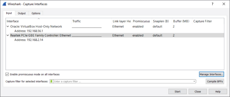
Figure 4-1: The Capture interfaces list
For a basic capture on your wired interface, the default options are okay; so, just click on eth0/em1 on Linux or Local Area Connection on Windows so that it is highlighted, and then click Start. By default, this sets the interface you selected to promiscuous mode (more on that later) and starts listening for traffic.
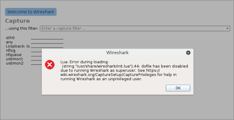
Figure 4-2: Superuser warning
After you start sniffing, you almost immediately begin seeing some traffic in the display, as most network-capable devices are constantly generating some traffic. You should click around on the packets shown in the packet list to familiarize yourself with the different panes of the interface and what kind of specific traffic you can see on your network.
As shown in Figure 4-3, packets are captured and displayed within the first seconds of sniffing. Clicking on packet number 7 on the Packet List pane, you see a breakdown of the packet in the Packet Details pane. In the Packet Details pane, you might expand any subtree by clicking the subtree's arrow on the immediate left. Note the arrow points right when the subtree is collapsed, and down when the subtree is expanded.
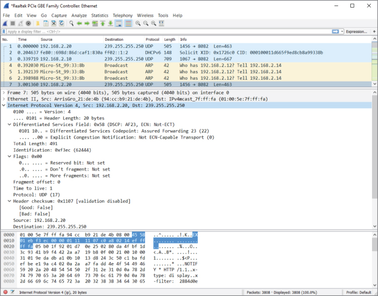
Figure 4-3: New traffic
You'll see by the example packet that the Packet List pane highlights which packet is being shown. The Packet Details pane shows inside the packet through the applicable subtrees. Expanding one subtree, “Internet Protocol Version 4,” in the Packet Details pane shows the packet's source and destination IP addresses, as well as various flags and other IPv4 header information.
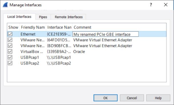
Figure 4-4: Renaming a network interface
Sniffing on Windows Versus Linux
To find the right interface in Windows, follow these steps:
- Open a command prompt by pressing the Windows key + x or by
searching for and executing cmd in the Cortana search box or the Run dialog box.
- Type ipconfig /all to list all the available network interfaces.
- Check each interface for the IP configuration of your network.
The name in the Wireshark list of interfaces corresponds with the name after “adapter” (for example, “Wi-Fi 4”).
To find the right interface in Linux, you follow similar steps:
- Open a terminal window.
- Type ifconfig /all to list all the available network interfaces.
- Check each interface for the IP configuration of the network.
Additionally, you can select Capture ⇨ Options within Wireshark to open the Capture Interfaces window. From there you can see each interface, a small graphic portrayal of traffic, whether or not the interface is in promiscuous mode, its buffer size, and other interface details.
For now, experiment with what you're able to see. The type of traffic you see in particular is, of course, somewhat limited to the traffic visible by your network interface. After a brief introduction to TShark, the command-line UI of Wireshark, we will delve deep into how to expand your visible traffic on the network.
TShark
TShark is the lesser known UI of Wireshark—and in my opinion is highly underused. TShark is for when you want to impress your friends by ripping out packets from a Linux terminal like an old-school Unix wizard. It is very similar in basic functionality to the revered tcpdump tool, but with all the added functionality of Wireshark, such as the easy packet filtering and the Lua scripting engine. In other words, it is tcpdump on steroids. When scripting for Wireshark, you usually end up using TShark, as opposed to the graphical interface, because it is more streamlined and better suited to further scripting. For this chapter, we focus on the basics needed to get packets scrolling across your terminal.
The following code illustrates a typical TShark session. The packets are numbered followed by timestamp, source and destination addresses, protocol, length, and description—very much like the Wireshark GUI but in a textual representation.
localhost:~$ tshark
31 5.064302000 192.168.178.30 -> 173.194.67.103 TCP 74 48231 > http [SYN] Seq=0
   Win=29200 Len=0 MSS=1460 SACK_PERM=1 TSval=926223 TSecr=0 WS=1024
32 5.074492000 192.168.178.30 -> 194.109.6.66 DNS 75 Standard query 0x56dc  A forums.kali.org
33 5.074987000 192.168.178.30 -> 46.51.197.88 TCP 74 59132 > https [SYN] Seq=0
   Win=29200 Len=0 MSS=1460 SACK_PERM=1 TSval=926226 TSecr=0 WS=1024
34 5.082801000 192.168.178.30 -> 46.228.47.115 TCP 74 33138 > http [SYN] Seq=0
   Win=29200 Len=0 MSS=1460 SACK_PERM=1 TSval=926228 TSecr=0 WS=1024
35 5.103958000 192.168.178.30 -> 91.198.174.192 TCP 66 47282 > http [ACK] Seq=1
   Ack=1 Win=29696 Len=0 TSval=926233 TSecr=3372083284
36 5.104123000 192.168.178.30 -> 173.194.67.103 TCP 66 48231 > http [ACK] Seq=1
   Ack=1 Win=29696 Len=0 TSval=926233 TSecr=1173326044
37 5.104411000 192.168.178.30 -> 91.198.174.192 HTTP 378 GE/favicon.ico HTTP /1.1
Like all the Wireshark tools, TShark runs on both Linux and Windows operating systems. With Windows, it isn't added to your working path, so you won't be able to run TShark from an open command prompt without first changing your working directory to the Wireshark installation folder. To avoid this little bit of extra typing, you can just add the Wireshark installation folder to your PATH variable, as outlined in Chapter 2.
Like most *nix command-line tools, supplying the -h flag displays some general help about how to use TShark. Additionally, if you want to check your version, and whether it supports Lua scripting, you can provide the -v flag:
localhost:~$ tshark -v
TShark 1.10.2 (SVN Rev 51934 from /trunk-1.10)
Copyright 1998-2013 Gerald Combs <gerald@wireshark.org> and contributors.
This is free software; see the source for copying conditions. There is NO
warranty; not even for MERCHANTABILITY or FITNESS FOR A PARTICULAR PURPOSE.
Compiled (32-bit) with GLib 2.32.4, with libpcap, with libz 1.2.7, with POSIX
capabilities (Linux), without libnl, with SMI 0.4.8, with c-ares 1.9.1, with
Lua 5.1, without Python, with GnuTLS 2.12.20, with Gcrypt 1.5.0, with MIT
Kerberos, with GeoIP.
Running on Linux 3.12-kali1-686-pae, with locale en_US.UTF-8, with libpcap
version 1.3.0, with libz 1.2.7.
Built using gcc 4.7.2.
The most important flag is going to be the -i flag, which specifies the interface on which to start capturing. Before the -i flag can be used, however, you will need to know how the interface you want to use is named. To help with figuring out which interface to use, TShark provides the -D flag. This flag prints all of the interfaces that are available for capture, as shown in the following code:
localhost:~$ tshark -D
1. em1
2. wlan1
3. vmnet1
4. wlan2
5. vmnet8
6. any (Pseudo-device that captures on all interfaces)
7. lo
To start capturing on a specific interface, use the -i flag along with the interface you are interested in capturing on. The -i flag is followed by either the specific interface or the number given by the list provided by the -D flag. If you do not specify an interface, TShark will begin capturing on the first non-loopback interface in the list. In the preceding example, the first non-loopback interface is em1. So, to capture on that interface, you would type:
localhost:~$ tshark -i em1
Capturing on em1
Frame 1: 66 bytes on wire (528 bits), 66 bytes captured (528 bits)
 on interface 0
Often, when scripting with TShark, you don't actually want to see all the packets that TShark is capturing because your script is already printing the data you want to see. Using the -q flag will suppress the majority of output so that you can clearly see the script output you are interested in. The reverse scenario is when you want to not just see what kinds of packets TShark is capturing but also the actual packet contents. Again, TShark provides the -V flag that will dump all the details of packets captured by TShark, as shown in the following example:
localhost:~$ tshark -V
Capturing on em1
Frame 1: 66 bytes on wire (528 bits), 66 bytes captured (528 bits) on
  interface 0
    Interface id: 0
    WTAP_ENCAP: 1
    Arrival Time: May 12, 2014 04:52:57.103458000 CDT
    [Time shift for this packet: 0.000000000 seconds]
    Epoch Time: 1399888377.103458000 seconds
    [Time delta from previous captured frame: 0.000000000 seconds]
    [Time delta from previous displayed frame: 0.000000000 seconds]
    [Time since reference or first frame: 0.000000000 seconds]
    Frame Number: 1
    Frame Length: 66 bytes (528 bits)
    Capture Length: 66 bytes (528 bits)
    [Frame is marked: False]
    [Frame is ignored: False]
    [Protocols in frame: eth:ip:tcp]
Ethernet II, Src: Alfa_6d:a0:65 (00:c0:ca:6d:a0:65), Dst: Tp-LinkT_eb:06:e8
  (00:1d:0f:eb:06:e8)
    Destination: Tp-LinkT_eb:06:e8 (00:1d:0f:eb:06:e8)
        Address: Tp-LinkT_eb:06:e8 (00:1d:0f:eb:06:e8)
        …. ..0. …. …. …. …. = LG bit: Globally unique address
  (factory default)
        …. …0 …. …. …. …. = IG bit: Individual address (unicast)
    Source: Alfa_6d:a0:65 (00:c0:ca:6d:a0:65)
        Address: Alfa_6d:a0:65 (00:c0:ca:6d:a0:65)
        …. ..0. …. …. …. …. = LG bit: Globally unique address
  (factory default)
        …. …0 …. …. …. …. = IG bit: Individual address (unicast)
    Type: IP (0x0800)
Internet Protocol Version 4, Src: 192.168.1.127 (192.168.1.127), Dst:
  64.4.44.84 (64.4.44.84)
    Version: 4
    Header length: 20 bytes
    Differentiated Services Field: 0x00 (DSCP 0x00: Default; ECN: 0x00: Not-ECT
   (Not ECN-Capable Transport))
        0000 00.. = Differentiated Services Codepoint: Default (0x00)
        …. ..00 = Explicit Congestion Notification: Not-ECT
  (Not ECN-Capable Transport) (0x00)
    Total Length: 52
    Identification: 0x46db (18139)
    Flags: 0x02 (Don't Fragment)
        0… …. = Reserved bit: Not set
        .1.. …. = Don't fragment: Set
        ..0. …. = More fragments: Not set
    Fragment offset: 0
    Time to live: 64
    Protocol: TCP (6)
    Header checksum: 0xc569 [correct]
        [Good: True]
        [Bad: False]
    Source: 192.168.1.127 (192.168.1.127)
    Destination: 64.4.44.84 (64.4.44.84)
    [Source GeoIP: Unknown]
    [Destination GeoIP: Unknown]
Transmission Control Protocol, Src Port: 53707 (53707), Dst Port: https (443),
   Seq: 1, Ack: 1, Len: 0
    Source port: 53707 (53707)
    Destination port: https (443)
    [Stream index: 0]
    Sequence number: 1    (relative sequence number)
    Acknowledgment number: 1    (relative ack number)
    Header length: 32 bytes
    Flags: 0x019 (FIN, PSH, ACK)
        000. …. …. = Reserved: Not set
        …0 …. …. = Nonce: Not set
        …. 0… …. = Congestion Window Reduced (CWR): Not set
        …. .0.. …. = ECN-Echo: Not set
        …. ..0. …. = Urgent: Not set
        …. …1 …. = Acknowledgment: Set
        …. …. 1… = Push: Set
        …. …. .0.. = Reset: Not set
        …. …. ..0. = Syn: Not set
        …. …. …1 = Fin: Set
            [Expert Info (Chat/Sequence): Connection finish (FIN)]
                [Message: Connection finish (FIN)]
                [Severity level: Chat]
                [Group: Sequence]
    Window size value: 41412
    [Calculated window size: 41412]
    [Window size scaling factor: -1 (unknown)]
    Checksum: 0x1917 [validation disabled]
        [Good Checksum: False]
        [Bad Checksum: False]
    Options: (12 bytes), No-Operation (NOP), No-Operation (NOP), Timestamps
        No-Operation (NOP)
            Type: 1
                0… …. = Copy on fragmentation: No
                .00. …. = Class: Control (0)
                …0 0001 = Number: No-Operation (NOP) (1)
        No-Operation (NOP)
            Type: 1
                0… …. = Copy on fragmentation: No
                .00. …. = Class: Control (0)
                …0 0001 = Number: No-Operation (NOP) (1)
        Timestamps: TSval 1972083, TSecr 326665960
            Kind: Timestamp (8)
            Length: 10
            Timestamp value: 1972083
            Timestamp echo reply: 326665960
Note that this is effectively what you see in the Wireshark GUI if you were to expand all the fields in the Packet Details pane. As you can imagine, with the -V flag set, any amount of network traffic will result in a fast-scrolling screen of capture output. If the volume of packets is too high to control, or if you discover packets are being dropped before they can be written to disk, remember that Wireshark allows you to change the buffer size. By default, the buffer is 2 MB for each interface. Increasing the buffer offers more room to scroll back for packet review.
This concludes the introduction to TShark. For the majority of the chapters, we'll use the GUI interface. Chapter 8 delves deep into programming with Lua, the scripting language that enables you to extend Wireshark, both at the command line and in the GUI. We also play a lot more with TShark.
Dealing with the Network
Earlier you experimented with a short capture (or is it still running?). Whether you use the Wireshark GUI or the TShark command-line interface, the packets visible to your device might be limited by the topology of your network. This is the common, fundamental challenge to anyone seeking to capture packets. And that's what this section is all about.
What good is a packet analyzer if you can't get the packets you want to analyze? The answer is pretty simple: It isn't! In this section, we go over different ways to capture packets to make sure you don't ever have the problem of not being able to get the network data you need for your task.
Capturing packets on Ethernet networks wasn't much of a problem until the rise of switched networks. Before the switch, the main tool for connecting multiple networked devices was a hub. A hub just copied every packet it received to all ports except the one it was received on to prevent loops. This meant everyone with enough privileges on a connected computer could capture all the traffic passing through the hub. Today it is more complicated; capturing packets requires anything from configuration changes to specialized equipment or dedicated packet-capturing features on network devices.
This section describes methods for capturing packets and, where applicable, provides explicit instructions on how to perform the capture. One warning, however: We are going to be talking about tools other than what is available with Wireshark. While this may seem blasphemous, we need to be clear on the Wireshark use case. The majority of Wireshark functionality is geared toward analyzing packets. Also, there are situations where you do not want to install any additional software but still need to gather packet data. We address these situations by discussing some other tools and scripts that are capable of recording a network into pcap format for later, offline analysis by Wireshark.
Local Machine
At times, it seems just capturing packets from your host machine isn't of much use, although you would be surprised at the information you can salvage from a network analyzer by just plugging it in and having it listen. Additionally, seeing what your network applications are actually doing on the network often tells you more than a thousand error messages can. In this section, we go over some techniques for capturing traffic on the local machine. In particular, we cover how to capture packets from the local machine using tools that are native to Windows and Linux as well as how to capture traffic that is just going over localhost.
Native Packet Capture
Native packet capture refers to capturing packets from a machine without having to install any additional tools. As mentioned in the introduction to this section, it is useful to be aware of the methods to capture traffic from a local machine without having to install additional software. A good example of a situation like this is when software is installed that prevents the installation or running of software that is not preapproved or included by default with the operating system installation. Another example is if you are trying to analyze a potentially compromised machine and want to avoid tipping your hand to the bad guy or muddling your results by installing additional software. Luckily, there are options for both Linux and Windows that enable you to get packet data without having to install any additional tools.
Native Windows Capture
We cover native packet capture in Windows first. Capturing traffic on Windows 10 and below without installing additional software is all but impossible. We don't say it is completely impossible, because if working in this industry has taught us anything, it is that anything is possible. The reason this is fortuitous is that newer versions of Windows actually provide functionality that can be leveraged to get packet captures without having to install any additional tools.
We are going to look at the netsh command-line tool. This tool has been available on Windows for several versions, and Windows 10 has only grown its feature set. In particular, it has the netsh trace command, which we will leverage to get some packet data.
There are a lot of awesome resources on the Internet for how you can really use netsh trace, so we are not going to go into too much detail of all the options this tool supports. For starters, at a command prompt, type netsh trace /? to view the options.
Sniffing Localhost
When we say localhost, we are usually talking about the loopback adapter, which is basically a virtual interface that isn't physically connected to an actual network. Localhost is actually just a hostname. By convention, however, localhost almost always resolves to the reserved 127.0.0.1 IPv4 address and the ::1 IPv6 address. Generally, applications use this loopback interface for inter-process communication between applications running on the same host machine.
Localhost is also often used by services that do not need to be exposed to a larger network. A prime example is a database server running on the same machine as the web application connecting to that database. Because the database is potentially accessible from outside of the web application machine, it poses a security risk. In such situations, simply bind the database to localhost so that the local web server can still communicate with it but the database is inaccessible from processes outside the local machine.
It should be noted that occasionally you will see applications that mess this up. For example, if your machine has an IP address of 192.168.56.101 and you bind a service to that IP specifically, then processes running on your local machine will be able to communicate with that service, much like they can if the service was bound to 127.0.0.1. The difference, however, is that anyone who can access the 192.168.56.101 from the local network at large can also interact with the service. This is why it is important to make sure that services that do not need to be exposed to the network at large are not binding to 0.0.0.0 (which is shorthand for all IP addresses) or any other interface that has a reachable IP address.
On Linux-based operating systems the loopback interface is generally the lo interface. Wireshark can easily attach to this interface and sniff packets destined to localhost only. Figure 4-5 shows some sample ICMP traffic to the IP address 127.0.0.1.
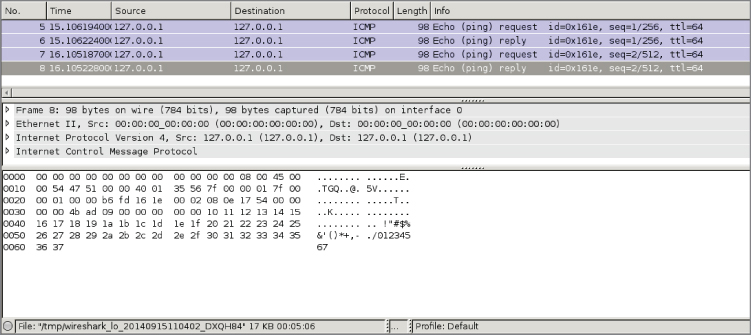
Figure 4-5: Sample localhost ICMP traffic
Windows and Localhost
In networking, every system has a hostname. The hostname identifies that specific system for services or connections. And while the hostname is unique compared to other systems, every system has the same name “local” to itself: localhost.
The hostname localhost refers to the system you're currently on. Connecting to localhost connects you to services running on the local system. If you have a web server running locally to serve the web files in a browser, simply type http://localhost to browse the locally running web service.
Similar to the local system's hostname, the network adapter used to connect to localhost is also special. It is called the loopback adapter. The loopback adapter is not a physical network adapter, but only a logical one. Wireshark is able to sniff and capture network traffic from the loopback adapter, provided it is installed. However, for Windows, the loopback adapter is not installed by default.
Adding a Loopback Adapter to Windows
The loopback adapter is not present by default on Windows systems. This does not mean that it is not using the loopback principle to transmit traffic to the local machine. To be able to capture this traffic, you need to add the loopback interface manually. Once the loopback adapter is available for Wireshark to present as an option, you can select it and capture from it.
Follow these steps to add the loopback interface to your Windows sniffing host:
- Run
hdwwizin a command prompt. This should open the Add Hardware Wizard. - Click Next and select the manual device selection option (Advanced).
- Select Network Adapters as the type of hardware and click Next.
- Select Microsoft as the manufacturer and select Microsoft Loopback Adapter as the network adapter (see Figure 4-6). Click Next.
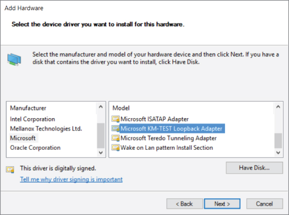
Figure 4-6: Installing the loopback adapter on Windows
- Click Next again to install the driver.
- Click Finish to close the Add Hardware Wizard.
You should now have a new interface using the loopback driver.
Sniffing without a Loopback Adapter on Windows
You can sniff traffic destined for the localhost on Windows without installing a loopback adapter. Netresec has a public tool called RawCap that can be used to sniff any interface on a Windows machine that has an IP address, and specifically can sniff traffic destined for 127.0.0.1. RawCap outputs to pcap format, which can then be easily loaded into Wireshark. You can review the RawCap web page on the Netresec site for a full explanation of how to use RawCap, but for our purposes we are just going to demonstrate how to use it to sniff localhost traffic. This is accomplished by double-clicking RawCap.exe, which displays the prompt shown in Figure 4-7. Select the appropriate network interface number—in this case, number 6 was chosen to sniff on the localhost. (Keep in mind that while it says Loopback, this isn't an interface installed on the machine, like in the previous section.) We then chose the name loopback_dump.pcap, which is saved in the current working directory.
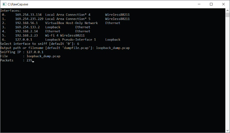
Figure 4-7: RawCap loopback sniffing
If you don't have any traffic on the localhost of your machine, you can generate some by pinging 127.0.0.1. After you capture a decent amount of traffic, press Ctrl+C to kill RawCap.exe and save your file. Figure 4-8 shows opening the pcap created by RawCap in Windows, which displays packets sent to localhost.
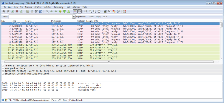
Figure 4-8: RawCap pcap in Wireshark
Sniffing on Virtual Machine Interfaces
Security researchers, whether offensive like pentesters or defensive like malware analysts, have a habit of using a lot of virtual machines (VMs). You generally carry only a laptop to the job, but you might need to reconstruct an entire network of computers to test something in your portable lab of VMs. You also almost always need varying versions of the most popular operating systems ready to go. Debugging complicated lab setups while testing your exploits or looking for vulnerabilities can take a lot of time. It always helps if you can take a look at what an application is actually doing on the network. This is especially helpful when error messages are missing and/or nondescriptive.
Which interface to sniff on in a VM environment depends a lot on your specific setup and the use case. Each of the common networking setups for VirtualBox is explored in detail in this section. Note that while other virtualization solutions may use different names for their network types, they are all generally implemented the same way, and the following information can be applied for how to capture traffic.
Bridge
Connecting your VMs with the bridged setup means connecting them on the same layer 2 network as your host machine. This means that the interface to which you have bridged will be responding to multiple MAC addresses—the MAC address of the physical interface as well as the MAC address for every virtual machine that has been bridged to the physical interface. All the traffic passing through the bridge can be sniffed on the interface to which the virtual machine has been bridged. This is especially useful if you are running multiple virtual machines and you want to see all the network traffic they are generating.
Figure 4-9 shows bridging a Kali Linux VM to a Windows host physical interface Realtek PCIe gigabit. Note the MAC address within the VirtualBox configuration window (which is configurable when the VM is powered off).
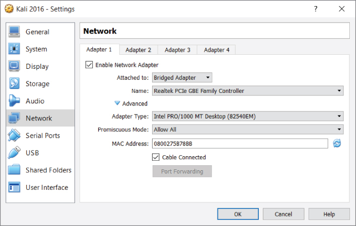
Figure 4-9: VirtualBox bridging
For my setup, the VM interface has an IP address of 192.168.2.12, and my host machine has an IP address of 192.168.2.14. Figure 4-10 shows the Wireshark output from the em1 interface (our host interface). These ICMP packets show that from a network standpoint the VM is attached to the physical interface and uses its own MAC address for Ethernet communication. Again, this means that as far as the network is concerned, there are two distinct Ethernet devices with only one physical interface.
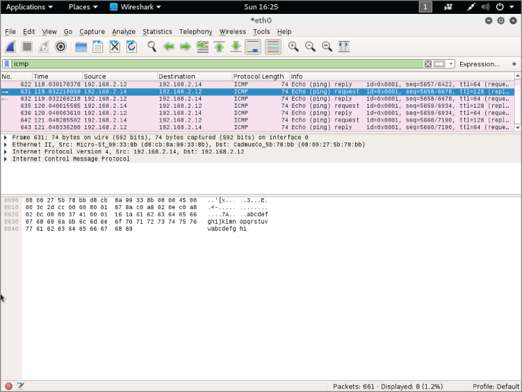
Figure 4-10: Wireshark sniffing bridged network
If you want to capture only VM traffic and not traffic generated by your actual host, you could use a capture filter. The following capture filter would apply to our previous example and capture only traffic destined for the Kali virtual machine:
ether src host d8:cb:8a:99:33:8b || ether dst host08:00:27:5b:78:bb
The downside is that you are exposing your VMs to whichever network the interface you have bridged is connected to. When deploying labs, you may want to ensure that the traffic is properly isolated, which is why you would use the host-only networking option, as discussed in the following section.
Host-only
For host-only networking in Oracle VirtualBox, a virtual network interface (for example, vboxnet0) is created on the host machine that acts as a switch. The VMs are then transparent to the host, attached to this virtual host-only switch interface. This is handy when you want communication between VMs and the host machine, such as virtual servers offered privately to the host. In host-only mode, the VMs do not have access to the Internet, like they do in a NAT network. Host-only mode is also commonly used when you are setting up a lab environment that you want to isolate for analysis. When using host-only networking, it is often helpful to sniff all the traffic of the host-only network traffic from the host itself. One would initially think that sniffing on the host-only network interface with Wireshark would give you all the traffic on the host-only network. Remember, however, that this interface is acting as a switch, so it only receives broadcast traffic or traffic that is actually destined for that host interface. Therefore, when sniffing from the host, you will not see traffic between VMs.
Obviously, you can run Wireshark within each VM to sniff traffic generated by that VM, but this gets cumbersome with a lab setup of more than two VMs. Unfortunately, there isn't an easy way to capture all the traffic on a host-only network. Because the unicast traffic between VirtualBox VMs connected as host-only mode cannot be captured by the host, VirtualBox offers a workaround (https://www.virtualbox.org/wiki/Network_tips). However, being a command-line solution and requiring effort on each VM to be captured, this is no simple fix.
You can create your own host-only network by using the Linux bridging utilities and running your own DHCP server, or by just using static IP addresses. We discuss Linux bridging in more detail later in this chapter.
NAT
Network address translation (NAT) is the default method of networking for connecting VMs to the outside world. When you configure NAT as the method for VM connections, your host machine is routing all the packets onto the network. It is a layer 3 connection, so you will not be able to analyze layer 2 traffic on the host side of the network. All traffic generated by your VMs will look like it originated from your host machine to the target network, and the VMs will receive all traffic forwarded by the host machine.
The NAT engine needs to keep track of all the connections made by the VMs in order to know where to send replies to these packets. This can generate problems when the VMs are generating a lot of connections (that is, port scanning). In these cases it might be a better idea to switch to bridged networking. If your network access is limited to one MAC address, for example, or if you change your network configuration repeatedly, it might save you trouble if you stick to NAT networking. This ensures the configuration for your virtual machines doesn't have to be updated each time you change networks, and it will fool the network into thinking only one machine is connected.
When you have a VM configured in NAT mode, you can sniff all the traffic the machine sends to the outside network by sniffing on whatever interface your default gateway is accessible on. The downside is that you are not able to easily distinguish between VMs, which are both using NAT. You also cannot easily distinguish between traffic generated by your host and those packets generated by VMs. Often NAT is useful only when you want to get access to the Internet from your VMs and you are not too concerned with getting good packet data from the traffic that VM sends.
Sniffing with Hubs
In the earlier days of networking, the typical method of connecting machines on a network was with a hub. Today's method is with a switch. As you know, the primary difference between switches and hubs is the traffic from one system is repeated out all other ports on a hub, whereas a switch is intelligent enough to direct the traffic only out the needed port. Switches learn what systems (known by their layer 2 MAC address) are hanging off of which ports. Hubs broadcast all traffic everywhere.
Remembering this key difference explains why sniffing with hubs means getting all the traffic, whereas sniffing off a switch can mean hearing only some of the conversation.
It's also important to remember the OSI model, the representative layering of how data travels and is handled between systems. Bits from the Physical layer get switched, routed, error-checked, authenticated, presented, and formatted, eventually leading to the top layer (Application). Discussion about switches and hubs is at layer 2, the Data Link layer, where network traffic is split into frames.
Switches versus Hubs
The difference between these two network devices was briefly mentioned in the introduction of this section. It boils down to the fact that a hub does not do anything intelligent with the frame. A hub operates on layer 1 (the Physical layer) of the OSI model. All bits are copied to every other port except the receiving one. This last bit of intelligence is essential in the case of two hubs connected to each other with one cable. If it would copy a broadcast frame to all ports, including the receiving one, it would cause a broadcast storm, amplifying that single broadcast frame.
Switches are more intelligent devices. They operate on layer 2 of the OSI model and thereby understand Ethernet (MAC) addresses. This enables a switch to decide to which port to send traffic by keeping a table that lists ports and MAC addresses. Broadcast frames are still forwarded to all ports except the receiving port. This behavior is the reason some (ethical) hackers still bring an old hub to consulting jobs. The fact that it keeps a table of MAC addresses means that you are not able to see traffic not addressed to you. This is generally a good thing, but not for those in the security crowd if they are investigating suspicious activity or are in an offensive role.
Sniffing from a Hub
To capture network traffic passing through a specific Ethernet cable, you need an Ethernet hub and two extra cables. After connecting all the cables, there is a Y-formed connection, as shown in Figure 4-11.
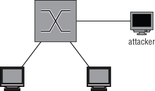
Figure 4-11: Capturing packets with a hub
Packets should now be repeated on all three sides of the connection. A few things have changed in the network, though. Most connections automatically negotiate their physical connections to full-duplex, allowing both transmitting and receiving at the same time when connected normally. When you connect a hub, all connections negotiate to half-duplex and therefore re-enable collision-detection protocols. This is an anomaly in modern switched networks. Full-duplex connections were not possible before switched networks because the collision domain of the connection contained more than one device.
As shown in Figure 4-12, a frame coming in to port number 1 will be duplicated to ports 2 and 3. This is similar to the behavior of a switch without Spanning Tree Protocol (STP) enabled, meaning all traffic is directed out, without regard to a possible looping.
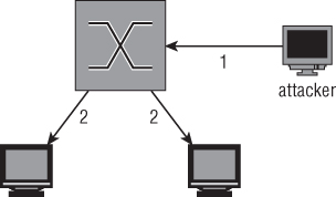
Figure 4-12: Traffic when sniffing on a hub
SPAN Ports
Switched Port Analyzer (SPAN) is a feature found on most managed switches or routers. Not every manufacturer uses the proprietary name SPAN, but the functionality is more or less the same. Another common term for the same principle is port mirroring. Sniffing on a SPAN port is explained in the following sections along with the configuration of a SPAN port on the most common network devices.
Sniffing on a SPAN Port
The traffic you see on your SPAN port depends on the configuration and capabilities of your capturing device. For this example, assume you want to capture the traffic of one device, as that is the simplest case.
Sniffing on the SPAN port is extremely versatile. Most of the time you can listen-enable the mirroring of packets from a list of interfaces or even an entire virtual LAN (VLAN). There is a serious pitfall, however: If you are sniffing multiple ports or an entire VLAN, there is a high chance you will get duplicate packets. This is a side effect of sniffing on a VLAN or multiple ports, so if you absolutely have to do this to capture all the traffic you need, there is no other option.
There is also the question of connectivity for the listening system. Depending on the vendor of the switch, connectivity may be disabled for a mirror destination port. This is a sensible default, because your own connectivity would only contaminate the network traffic you are capturing, which could be problematic in a mobile pen-testing scenario. So, be prepared and investigate the options your switch supports.
Figure 4-13 shows a diagram of the connections in a SPAN-sniffing setup. The dotted line represents the copied packet originally destined for another client also being transmitted to the attacker.
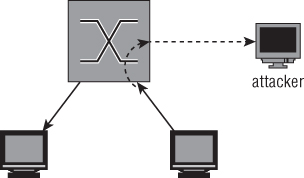
Figure 4-13: SPAN sniffing connections
Configuring SPAN on Cisco
To monitor all the traffic coming in or out from FastEthernet port 1/1, use the following snippet. This is the syntax for most of the Catalyst series of Cisco switches:
Switch#conf t
Switch(config)#monitor session 1 source interface fastethernet 1/1
Switch(config)#monitor session 1 destination interface fastethernet 1/2
Switch(config)#exit
You can check the results of your commands with the following:
show monitor session 1.
By default, there are two assumptions in the previous configuration. The first monitor statement assumes that both directions should be monitored. This can be overridden by specifying both | rx | tx. The second assumption is probably less expected. In a Cisco SPAN configuration, a destination monitor port by default does not accept any incoming traffic. You are only able to receive the monitored traffic, and no connection to the network can be made. To enable incoming traffic on the destination port, you can append ingress vlan vlanid to specify the VLAN incoming traffic should be sent to. For example, to capture traffic received on the monitored port and allow normal traffic on the destination port, enter the following:
Switch(config)#monitor session 1 source interface fastethernet 1/1 rx
Switch(config)#monitor session 1 destination interface fastethernet 1/2
                                             ingress vlan 5
Switch(config)#exit
Different models of the Catalyst switch series will have different syntax. Cisco routers are also not covered by this example. The general idea will be the same, however, so refer to the references and examples from Cisco if you are trying to configure port mirroring on a specific model and the previous examples do not seem to apply.
Configuring SPAN on HP
HP ProCurves are a common alternative to Cisco or Juniper network hardware. Their syntax is similar to Cisco, but there are small differences as well as completely different terms for the same features.
The following statements enable port mirroring on an HP switch:
Procurve(config)# mirror-port 6
Procurve(config)# interface 2
Procurve(eth-2)# monitor
Procurve(eth-2)# exit
Procurve(config)#
In this case, port 6 is the port where monitored traffic is duplicated. You can specify the monitor keyword for multiple interfaces. All the traffic will be sent to the mirror port. In the switch we used for testing, it was impossible to specify only capturing sent or received packets.
You can show the current monitoring configuration by executing:
Procurve# show monitor
The output will show both a list of ports being monitored as well as the interface the packets are being mirrored to.
Remote Spanning
Sometimes the person responsible for analyzing spanned traffic is unable to have the monitoring device directly off of the spanned port. In another case, a person might want to monitor spanned ports on more than one switch. In both cases, you just need to use remote spanning. Remote spanning allows you to monitor a switch port from a device on another switch port. And you can set up remote spanning to span ports from multiple switches. In both cases, the spanned traffic gets sent to the destination switch port (typically over a dedicated VLAN to isolate the traffic and prevent possible collision or loop issues). The monitoring device is expected at the destination port.
Network Taps
Network taps are devices dedicated to capturing traffic on a network. They are available for different types of networks and/or cables used. A lot of network taps are passive devices, meaning they perform the capture without any software or intelligence by making a bypass connection to the RX wire pair, for example.
Because you are tapping into a network line and not as a connected device, there might be some confusion about the direction of traffic. Be assured that, even when connected only to the RX wire pair, you are still capturing traffic intended for all. The bits are still traveling on the wire, regardless of what originating device's traffic you are capturing. If you choose to aggregate traffic, then also be mindful of how much traffic you're receiving. If your tap is more than 50% utilized, you're likely dropping packets.
Unlike SPAN ports, taps can capture network traffic at 100% utilization very well. This is in part due to the fact that a tap does not change in the operation of the network (aside from the fact that it leaks traffic to someone other than the intended recipient).
A tap generally does not combine the mirrored traffic into one port for easy sniffing. It merely replicates incoming traffic on both of the interfaces to separate monitoring ports. In order to capture all traffic on a tapped link, you need two sniffing interfaces on your monitoring workstation.
There are a few advantages to using taps compared to other methods of capturing network traffic. Because most taps are passive devices, it is unlikely they will disrupt network connectivity because of hardware failure. For the same reason, they are completely invisible on the network. They do not participate on the network, so they cannot be detected or change its behavior, except on negligible physical levels (for example, degrading signal quality).
Most passive network taps degrade the connection to 100BASE-TX on purpose because a passive device cannot tap a 1000BASE-T connection. This is due to the fact that it uses all four wire pairs and auto-negotiates a clock source. A passive tap might allow two devices to continue operating on 1000BASE-T but would not be able to sniff the packets because it would be unaware of the clock source. Active switches solve this problem and allow you to capture up to 10GBASE-T, while keeping the redundancy features that do not interrupt the connection when the device fails.
For the reasons just mentioned, taps are useful for applications like intrusion detection systems and similar monitoring, where the traffic only needs to be read.
Professional-Grade Taps
An enterprise-level network tap is an expensive network device that can be rack mounted most of the time, just like any other high-capacity network device. This makes these types of taps a good fit for permanent sniffing solutions as might be needed for an IDS. These taps can often be configured dynamically, and most claim not to interrupt the tapped connection in the event of device or power failure.
The use of these taps as well as an overview of the types available is out of the scope of this book. Suffice to say that these devices are available in all types and flavors for every physical network media in use in modern networks.
Throwing Star LAN Taps
The throwing star is a popular LAN tap available either in kit form to assemble yourself or as an assembled device. It is completely passive and quite inexpensive. It is primarily used by enthusiasts and is a common addition to the pentester's kit bag.
As shown in Figure 4-14, the throwing star is a portable device, so there is no excuse for not keeping it in your set of default equipment. Like the other types of passive Ethernet taps, the throwing star splits the Rx and Tx traffic to separate Ethernet cables. It also uses its circuitry to force the speed to auto-negotiate to 100 Mbps in order for the wiring to be correct, as described earlier in this section.
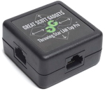
Figure 4-14: Throwing star LAN tap
Source: Great Scott Designs
Transparent Linux Bridges
If you own a machine capable of running Linux with two or more network interfaces, you can transform it into a powerful networking tool. This section shows you the basics of Linux bridges and how to sniff traffic with them.
Using a bridge is very versatile because you can use packet filtering provided by the operating system. This allows you to block certain traffic or even change packets and redirect them to a malicious destination, which is covered in Chapter 6 when dealing with man-in-the-middle attacks.
Sniffing on a Linux Bridge
Linux bridge support is built into the Kernel, but to start using it you need to install the support utilities. For Debian/Ubuntu-based systems, install the package bridge-utils:
localhost# apt-get install bridge-utils
And do the following for Red-Hat based systems:
localhost# yum install bridge-utils
After installing the bridging utilities, yo can manage bridges by using the brctl command. This command allows you to add a bridge with the addbr command, which appears as an extra interface. Then you use the addif or delif commands to add interfaces to the bridge. If the interfaces are up and in promiscuous mode, packets will be forwarded between the interfaces.
To create a bridge named testbr using eth1 and eth2 of your machine, use the following commands:
root@pickaxe:~# brctl addbr testbr
root@pickaxe:~# brctl addif testbr eth1
root@pickaxe:~# brctl addif testbr eth2
root@pickaxe:~# ifconfig eth1 up promiscuous
root@pickaxe:~# ifconfig eth2 up promiscuous
root@pickaxe:~# ifconfig testbr up
Packets should now be forwarded from one interface to the other. This also means that the packets being processed by your machine can now be sniffed. All you have to do is set up Wireshark to listen on the bridge with a device directly attached to it, and it will receive every packet that passes through. Figure 4-15 illustrates the flow of traffic.
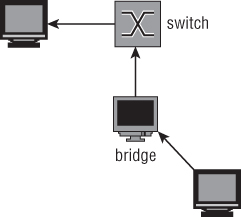
Figure 4-15: Traffic flow when sniffing a Linux bridge
Hiding the Bridge
In the default configuration, a Linux bridge is not the stealthiest of options. A number of issues might negatively affect the network you are sniffing, contaminate your traffic samples, or give away your presence. This section highlights some of the troubles you might encounter while trying to sniff using a transparent Linux bridge.
Linux bridges support Spanning Tree Protocol (STP). STP uses Bridge Protocol Data Unit (BPDU) packets to detect loops in the network. BPDU packets can be thought of as scouts sent to detect anomalies, particularly loops, in the topology. Loops in a network are very bad because broadcast packets can propagate around and get re-sent, cascading into a network-crippling broadcast storm. BPDU packets that detect a loop will instruct the STP-enabled switch to disable the offending switch port. If you connect a switch for the purpose of sniffing, you generally do not want this feature, especially if you are sniffing a workstation or similar non-networking device that would not send BPDU packets in normal operation. For these reasons, you should verify that STP is disabled on your bridge.
The following code snippet shows how you can check if STP is enabled and how to disable it:
root@pickaxe:~# brctl show
bridge name  bridge id            STP enabled   interfaces
stpbr        8000.000000000000    yes
root@pickaxe:~# brctl stp stpbr off
root@pickaxe:~#
A cautionary note: A bridge interface generates traffic. Traffic originating from the bridge will have layer 2 (MAC) information in the IP header. Even when you don't configure an IP address on the bridge, it can generate traffic in some cases. Unless you specifically configured your bridge to run in a “transparent” mode or “stealth” mode, your bridge's MAC information will be used. This traffic not only gives away your presence on the network, but traffic with an unfamiliar MAC address might even disable the switchport if the settings are restrictive enough or if there is a form of Network Access Control (NAC) in place. A good way to prevent these problems is by filtering all traffic from the host going out the bridge entirely using iptables.
The following iptables statements block all outgoing traffic originating from the host. This has to be done on the bridge interfaces as well because some kernel modules (like the IPv6 stack) generate traffic on all connected interfaces in an attempt to autoconfigure or because of multicast protocols.
root@pickaxe:~# iptables -A OUTPUT -o stpbr -j DROP
root@pickaxe:~# iptables -A OUTPUT -o eth1 -j DROP
root@pickaxe:~# iptables -A OUTPUT -o eth2 -j DROP
Remember that this disables your connection to the network if you are using the bridging interfaces for other purposes (like browsing the Internet). If it is essential for you to be stealthy, take extra care to disable IPv6 functions that try to automatically configure. It is best to disable IPv6 altogether in a sniffing setup because it is hard to limit the transmission of packets on an IPv6 interface that are related to the IP protocol itself.
Wireless Networks
Wireless communications result in unique challenges to safeguard confidentiality. A cable gives at least some idea of the recipient. In the case of wireless communications, the recipient can be anywhere within a given radius. For this reason, there are multiple ways to secure the packets traveling through the airwaves. Some of these protocols have been broken, exposing the users of these deprecated protocols to sniffing. Others choose to leave the WiFi Access Points unsecured for ease of access or to run a restaurant hotspot. The full scope of sniffing wireless networks is beyond this book, but this section gives you a primer on the possibilities when sniffing WiFi connections.
WiFi sniffing on Windows is very challenging because WinPcap, the library used by Wireshark, does not support monitor mode, also called rfmon mode for wireless. If you need a monitor mode for Wireshark on Windows, you will need to change the driver, at a minimum. At the time of this writing, one possible driver option is Riverbed AirPcap. In general, getting wireless monitoring working in Wireshark is highly dependent on the version of Windows, Wireshark, the model of wireless adapter, and, of course, the driver. Therefore, this section focuses on sniffing wireless connections on Linux.
Unsecured WiFi
Transmitting packets through an unsecured wireless connection is much like a shouting conversation across a city square: You can't really blame people for listening in. The same applies to sniffing on a wireless link. All you need is a wireless network card that supports promiscuous mode to hear everything that is shouted across that busy café hotspot.
Promiscuous mode for a wireless card is called monitor mode or rfmon mode. The easiest way to check if your wireless card supports this mode, and to enable it if it does, is the Aircrack-ng suite of tools. Go to http://www.aircrack-ng.org/doku.php?id=faq for up-to-date information. Currently, an expensive but known working option is the Alfa AWUS036H, a USB wireless card with high output that makes it ideally suited for sniffing and security applications.
Follow these steps to enable monitor mode on your wireless interface and analyze the packets with Wireshark:
- Connect the WiFi card. Make sure it is detected in
dmesgoutput. - Disable all programs that might interfere with the card's operation (for example, dhclient and NetworkManager). Airmon-ng will also warn you about this.
- Execute the following command:
airmon-ngwlan0start(wherewlan0is the name of your supported wireless card). Note that you will have to run this command as root. - Airmon-ng creates a new interface called mon0.
- Start Wireshark and select the new interface mon0 to sniff the packets in Wireshark.
As shown in Figure 4-16, Wireshark shows you all the raw packets it receives. In the case of unsecured WiFi connections, as used in public hotspots, this means you can see all the traffic if the signal quality is good enough.
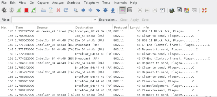
Figure 4-16: Raw wireless packets in Wireshark
Identifying base stations with airodump is also possible. Using the tool airodump is left outside the scope of this book, as there are several resources online.
The wireless card is tuned to a specific channel and you will only see packets that are transmitted in the frequency range belonging to that channel. The allowed channel numbers differ by region but are in the range of 1 to 14. To change the channel the card is listening to, use the following command:
root@pickaxe:~# iwconfig channel 6
Loading and Saving Capture Files
Viewing packets in the GUI using Wireshark or watching them scrolling by you in TShark is great. Sometimes, however, Wireshark isn't the only tool you want to use for packet analysis. Packet captures can come from varying sources generated by different tools and saved to different formats. Wireshark supports both saving out to the common pcap formats and reading/saving various proprietary formats.
You cannot save a running capture, so in order to save your traffic, you need to stop the capture using the menu or by clicking the Stop button in the toolbar; otherwise, the Save button or menu options are grayed out. After stopping a running capture session, you can save it by selecting File ⇨ Save or pressing Ctrl+S. This presents a Save dialog box, where you can select the filename, destination path, and output format for the packet capture.
Likewise, there are very interesting packet captures available online for loading and analyzing. While most traces are kept at a minimal size and common format, you might find a few needing extra attention.
File Formats
Since Wireshark version 1.8, the default output format is PcapNG, a newer format being developed by WinPcap. PcapNG has support for saving metadata in the capture file, such as comments; it also supports higher precision timestamps and name resolution. If you intend to view the capture with a different, much older tool, you will want to save in the older pcap format to ensure compatibility. As shown in Figure 4-17, Wireshark can support file formats for a wide range of tools.
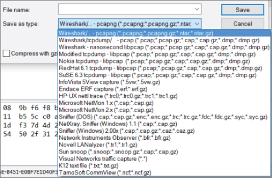
Figure 4-17: The File Save dialog box
Table 4-1 summarizes the different formats that Wireshark supports. Depending on which version Wireshark is running or produced the capture file, the capture will be one of the two primary supported file formats.
Table 4-1: Common Wireshark Capture File Formats
| FORMAT/EXTENSION | INFORMATION | SUPPORT |
| PcapNG | This is the next-generation format supported by libpcap from version 1.1.0 and onward. | New default for Wireshark, tcpdump, and other tools using libpcap. |
| Pcap | The original pcap format. | This is the most supported pcap format, as all tools using libpcap will be able to parse it. |
| Vendor-specific formats | Wireshark supports a good portion of capture formats available from specific vendors or programs — IBM iSeries, Windows Network Monitor, and so on. | Highly specific to the vendor. |
With a capture file loaded, it is easy to find out a capture file's format. In Wireshark, click on Statistics and choose Capture File Properties. The properties of the capture file will appear in a new dialog box (see Figure 4-18).
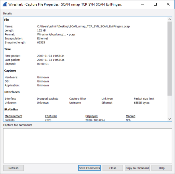
Figure 4-18: Properties of a capture file
Additionally, at the command line, you can type capinfos, followed by the capture file in question, to report file information.
Effectively, pcap is a means of serializing network traffic data, although it can be used to serialize anything. It is just an ordering of bytes that are given meaning by the standard. A good reference for the pcap format is on the Wireshark wiki, at https://wiki.wireshark.org/Development/LibpcapFileFormat. It is actually a pretty simple file format. There is a global header that includes a magic number (how applications identify it is a pcap file), the version of pcap the file is in, time zone offset, the accuracy of the timestamps (for example seconds versus microseconds), the snap length, which is the amount of data to capture for each packet, and, finally, the type of network the packet data was captured from (Ethernet, IP, and so on).
This global header is then followed by the packet header of the first packet. There is a packet header for each packet captured. The packet header contains metadata about the packet, such as the timestamp in seconds and microseconds, length of the packet data captured, and actual length of the packet. If you remember earlier, this explains why the Packet Details pane contains a Frame column that tells you the number of bytes captured versus the number of bytes that were actually transmitted. Wireshark is able to parse this all out from the pcap file. After the pcap header you have the actual packet/frame data. What is awesome about pcap is that it is actually a really simple format, which means it is easy to build your own pcap files even without some sort of high-level library. This is actually the approach we took for some of the custom sniffing applications developed during this book.
Now that you understand pcap, it should be clear that when doing live sniffing, Wireshark is reading in pcap-formatted data from Dumpcap. How Dumpcap gets data from the actual network card differs depending on the operating system and even the network type and network card being used. In Windows, you are almost always going to be using WinPcap. WinPcap is the library that allows you to actually capture raw packet data from your network card and then formats it into the pcap format. In Windows, Dumpcap is going to be using the WinPcap library, whereas on Linux it is generally going to use libpcap. Libpcap is the original packet capture library, used for virtually any *nix systems and is a programming library that allows you to get raw network data formatted into pcap. (libpcap developers actually invented the pcap format.)
Ring Buffers and Multiple Files
Wireshark is capable of spreading the captured data over multiple capture files. This is good when you intend to keep the capture running for some time or when you know you are going to be capturing a lot of traffic. Working with multiple, smaller capture files is far easier than wrestling with a resource intensive, large or ongoing packet capture. And waiting for a very large capture file to open or save out to the hard drive can eat up precious time and resources as well. Finally, if you're planning to continuously capture, then saving to multiple files allows you to work with one file or share it with a coworker, all without interrupting the ongoing packet capture.
Configuring Multiple Files
Spreading a capture over multiple files can be handy for a few reasons. Disk space may be scarce, for example, or you may need only recent traffic for your analysis. You might want to e-mail a capture file but need to divide it to be a maximum size. Or perhaps you're dealing with an extreme amount of traffic or need files to be divided often. Think of the reasons that would apply to you when deciding how large or how often you want to divide the captures.
Wireshark offers you the chance to divide files by size (KB, MB, or GB) and/or by time (seconds, minutes, or hours). You can set it to divide by one or both conditions. Once the file exceeds either condition you select, the file is saved and a new capture file begins.
To configure saving to multiple files (with or without a ring buffer), follow these steps:
- Open the Capture Options dialog box by selecting an interface and clicking Capture, then selecting Options.
- In the Capture Options dialog box, select the Output tab.
- Enter a base filename by clicking Browse and typing a filename and path. (A filename is required.)
- Configure the options you want to use. (We select every 5 megabytes or every 5 minutes, whichever happens first.)
- Click Start to start capturing.
The steps we did are shown in Figure 4-19. After clicking Start, you begin seeing packets scrolling up the Packet List pane. Wireshark is recording packets (capturing them) and saving them to the first capture file. If you chose to use multiple files, the capture continues until the first capture file is complete. A file completes when it reaches a certain size or after the set time has passed, depending on the chosen option.
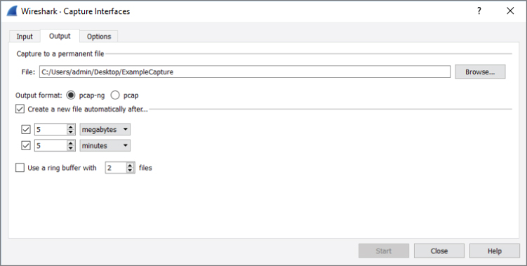
Figure 4-19: Multiple file settings
After the first capture file is finished, a new capture file begins. The scrolling packets in the Packet List pane does clear and reset, but no packets are lost in the capture process. Capturing continues for as long as you configured.
Finally, if you click the Options tab in the Wireshark: Capture Interfaces dialog box, you will see additional options to limit your capture, as shown in Figure 4-20. You can instruct Wireshark to stop capturing after it reaches a number of files, or the files reach a certain size or after so much time. You can even instruct capturing to stop after a set number of packets is reached.
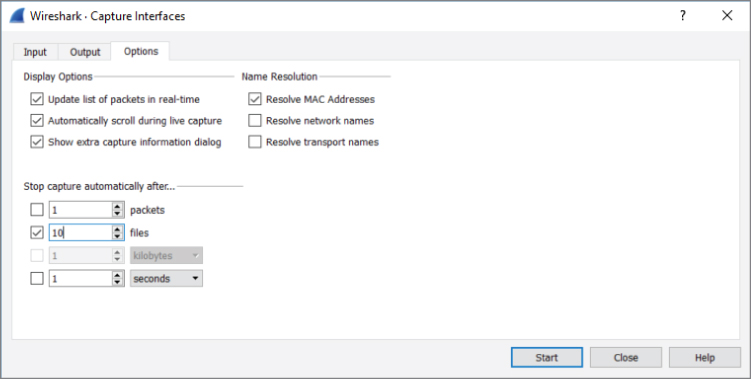
Figure 4-20: Stop capture options
Configuring a Ring Buffer
In addition to saving to multiple files, Wireshark can also use a ring buffer of multiple files to save the last megabytes of data captured or packets captured within a certain time period. This mode starts saving to a new file after a set amount of traffic has been captured or amount of time has passed, depending on your configuration. After you reach your chosen number of buffer files, the next saved file writes over the oldest buffer file. This process loops to keep the number of buffer files containing the most recent packet captures.
Let's put all this information to good use in an example.
You need to create a new file after every 10 seconds, with the base file name “10SecRing” to save on the desktop. Then, you also enable the ring buffer for a ring of five files. To see all those settings in place, refer to Figure 4-21.
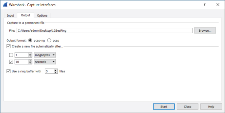
Figure 4-21: Setting multiple files and ring buffer
From this dialog box, start the capture immediately by clicking Start. After every 10 seconds, the Packet List pane clears for a brief moment, hinting the capture just started a new file. No packets are dropped in the course of closing one file and reopening another.
Wireshark will continue to make new capture files until the ring buffer's threshold is reached. By choosing a ring buffer of five files, the sixth capture file will overwrite the first capture file. You will have a ring buffer of five full files containing the most recent packets captured. Again, multiple files are named with incrementing numbers and with the start time of the capture.
After more than a minute, stop the capture.
As shown in Figure 4-22, you have the five ring buffer files. Note the filenames include a date and time stamp, beginning with the base name and sequential number. Also note the five files are now numbered 00003-00007, because after 50 seconds, the first file was overwritten and it continues in that manner.
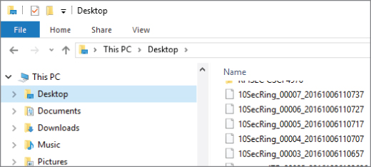
Figure 4-22: Resultant ring buffer files
Merging Multiple Files
You might opt to merge two or more capture files together. While the GUI offers the option under File to merge capture files, it is easier and more flexible to use the command-line tool mergecap. Mergecap is part of the Wireshark distribution. If you are using Windows, you'll find mergecap in the Wireshark directory.
For example, let's merge three of the 10SecRing capture files into one 30-second capture file. For this example, we'll use Windows.
- Open a command window and run as Administrator.
- Set a path for Windows to find mergecap. This is done with the command
set PATH=%PATH%;"c:\Program Files\Wireshark"(if you installed Wireshark in the default location). - Go to the location of your capture files to be merged and use the following command and syntax:
mergecap -w 30SecCap 10SecRing_00003_20161006110657
10SecRing_00004_20161006110707 10SecRing_00005_20161006110717
The -w switch tells mergecap to output as a file, named “30SecCap” in our case. You follow the output file with the files to be merged. That's it!
If you use the -v verbose switch, mergecap will tell you the format type of each file, pcapng in our case, as shown in Figure 4-23. (Be careful if you're merging a million packets, however; verbose will echo that each record is merged, every step of the way!)
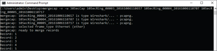
Figure 4-23: Mergecap verbose
In the end, mergecap will humbly echo it's complete (see Figure 4-24).
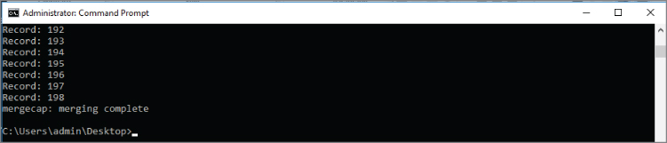
Figure 4-24: Mergecap complete
It's important to note that you do not have to merge capture files that are perfectly adjacent to each other with respect to time. For example, you can merge capture files from different days together. Wireshark will set the timestamps relative to each other chronologically.
Recent Capture Files
The first time you launch Wireshark, you see the list of network interfaces. You pick the interface here or you can choose it within Wireshark under Capture ![]() Options. Let's assume you've already captured packets and then saved to a file.
Options. Let's assume you've already captured packets and then saved to a file.
The next time you open Wireshark, the interfaces are no longer the top item shown. Now it's a list of capture files recently opened or saved. This list, under the heading Open, is shown above the Capture heading with the interfaces. The list of recently opened capture files shows the path of the capture file, the name, and total size. This list will continue to grow to the maximum allowed number. If too many are present, just scroll down to select the capture file you want. Wireshark obviously confirms file availability, because for any captures not available, the full path and filename will be italicized, followed by “(not found)”.
Clearing or Stopping the Recent Files
Maybe you don't want recent capture files showing up there. Because maybe you don't want a client shoulder-surfing as you open Wireshark, spotting the names of another client's traces or seeing filenames suggesting problems. In any case, the list of recent captures can pose a confidentiality risk.
It's a simple few clicks to clear out the list of recent files. Once in Wireshark, click File on the top menu bar, then Open Recent. At the bottom of the recent file choices, you will see Clear Menu, as shown in Figure 4-25.
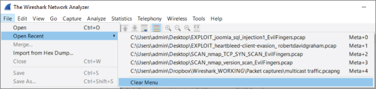
Figure 4-25: Clearing recent files
If you want fewer recent files to show, or perhaps none at all, click Edit on the top menu, then Preferences. In the Appearance menu, you can use the Show up to option to select the number of recent files to display (see Figure 4-26).
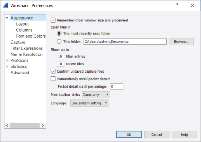
Figure 4-26: Changing the number of recent files shown
Dissectors
Dissectors are the magic that changes the bytes on the wire to the rich information displayed in the UI. Dissectors are one of the most important features that make Wireshark the powerful tool it is. Each protocol is parsed by a dissector and passed on to the next dissector until everything up to the Application layer has been converted from bits and bytes to all the separate fields and human-readable descriptions that are presented in the different parts of the UI. Dissectors are also what define the fields that allow you to apply the various filters. (Filters are discussed in more detail later in this chapter.) For now, this section serves as a quick introduction to dissectors. Chapter 8 walks through creating custom dissectors to parse custom protocols.
The first dissector is always the Frame dissector. It adds the timestamps and passes the raw bytes to the next-lowest protocol dissector—usually Ethernet. Wireshark uses a combination of tables containing which protocols are built on top of which other protocols combined with heuristics like port numbers to decide which dissector to apply to a packet. Some protocols, like Ethernet, have a field that states which protocol it is encapsulating, so heuristics are not needed and Wireshark can easily pick the right dissector for the job.
In basic Wireshark traffic analysis, you won't need to tweak anything about dissectors. You will occasionally come across a scenario where Wireshark isn't able to determine the appropriate dissector to use. This often happens with HTTP traffic over a nonstandard port.
W4SP Lab: Managing Nonstandard HTTP Traffic
An example of HTTP traffic over a nonstandard port is provided for you in the Wireshark for Security Professionals (W4SP) Lab. In the virtual lab environment, the server FTP1 is serving web traffic over TCP port 1080. Capturing traffic in Wireshark will present that traffic incorrectly. You need to alter the way Wireshark interprets the traffic so that the protocol is correctly labeled in the Packet List pane.
With this example, the packets will usually be shown as just type TCP because that was the highest level protocol that Wireshark can immediately identify. If you want to tell Wireshark it has to use the HTTP dissector on traffic, you will need to add a dissection rule.
Our example has captured some HTTP traffic that is going over port 1080. In this case, however, Wireshark confused the traffic as Socks, as the default port for Socks traffic is 1080. To solve this dilemma, a new dissection rule is applied. To add a dissection rule, select a packet and choose Analyze ![]() Decode As, or right-click one of the packets you want to change the decoding of and select Decode As. Figure 4-27 shows this process with the Decode As window.
Decode As, or right-click one of the packets you want to change the decoding of and select Decode As. Figure 4-27 shows this process with the Decode As window.
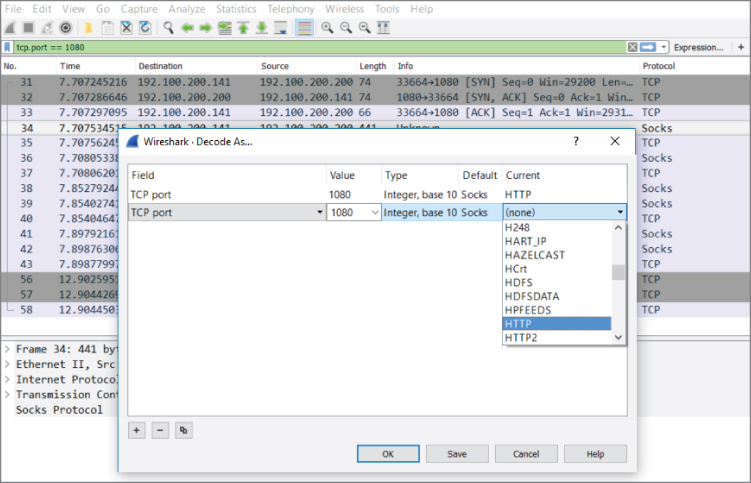
Figure 4-27: Wireshark's Decode As window
To apply the HTTP dissector to the TCP stream, select HTTP from the available protocol choices to tell Wireshark to apply the dissector to TCP traffic that is using the port 1080. Click OK to save your settings. When you return to the Packet List pane, Wireshark is now able to identify the HTTP traffic correctly. Figure 4-28 shows that we've told Wireshark to correctly decode the traffic over 1080/tcp as HTTP.
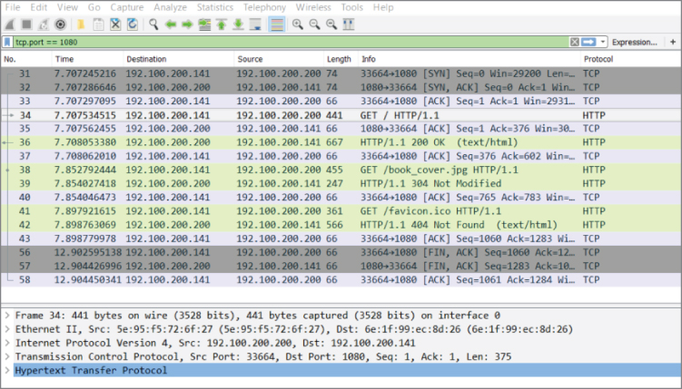
Figure 4-28: Wireshark's Decode As window
Filtering SMB Filenames
Server Message Block (SMB) is a good protocol for a practical example. Every network with some Windows clients will have some SMB activity, especially when a domain is set up and the clients are connected to various network shares. This section illustrates the process in which a filter evolves. The process used within this section can be applied to any other type of scenario where you have a packet field you want focus on. Notice that you don't necessarily need to read any RFCs or reverse engineer the protocol. The Wireshark dissector has done all the heavy lifting for you in this case, and all you need to do is figure out how to build the appropriate filter.
To start, packets are scrolling by too fast to read. Most of it is HTTP traffic with an occasional burst of SMB with a spattering of ARP and DHCP broadcasts. Suppose you have been tasked to figure out which files are being accessed over SMB. You are focusing on SMB traffic, so the logical first step is to filter for it by using smb as the filter. For new versions of Windows, such as in Figure 4-29, you will use smb2 as the filter.
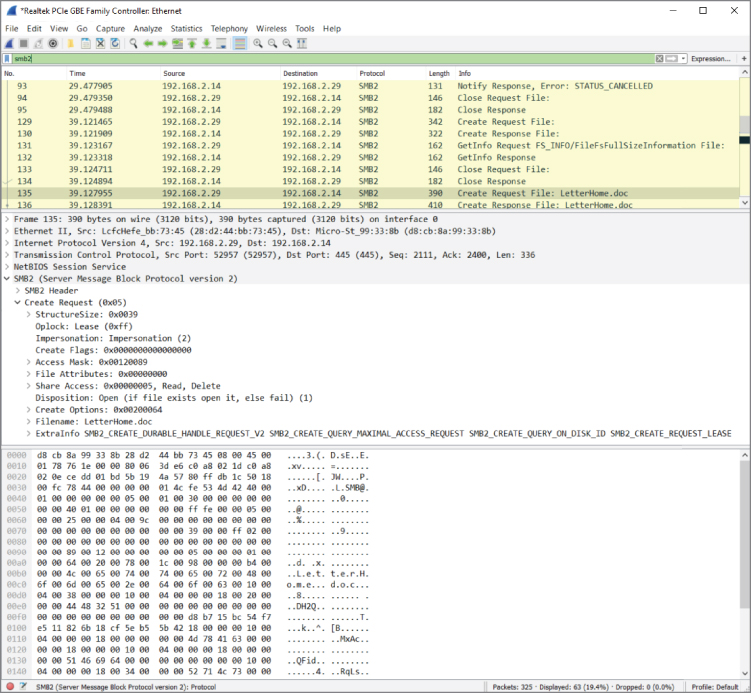
Figure 4-29: Packet list filtering for SMB
Not all the SMB packets you see now are the result of the computer accessing files. In fact, probably only a fraction of the packets are even accessing a file. The rest are concerned with metadata, directory listings, and just general protocol overhead. The packet list in Figure 4-29 has what appears to be a path in the description and would therefore serve as a good starting point for further investigation. Because you are looking for filenames being accessed, you should find differentiating properties for this SMB packet so that you can filter for all the packets concerned with a filename or path. If you look at the Packet Bytes pane, the filename is obviously in there. There is a little trick here: When you click on the filename in the Packet Bytes hexadecimal display, Wireshark will highlight the corresponding object in the Packet Details pane. If it highlights the entire Trans2 object, just expand it until you see the corresponding field. The corresponding filter field for this file attribute is smb2.filename, so this is the filter you can apply next. This filter has narrowed the list of packets down to all the SMB requests that reference a file. Sounds pretty close, right? The Packet List pane should now look somewhat like Figure 4-30.
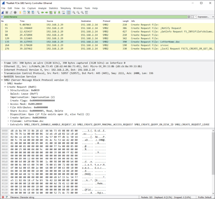
Figure 4-30: SMB packets referencing a file
To narrow it down further, you need to determine what sequence of packets forms the transaction of accessing a file with SMB. The quickest way to do this is to control the actions of the client by copying a file from a share and tracing this in Wireshark. The best way is to consult reference documentation for the protocols you are analyzing, but generally time is against you in the security field and you may encounter protocols that are not that well documented. To see the packets concerned with copying your file, use the filter smb.file contains"partoffilename". Using this relatively limited set of packets, the types of packets in a transaction can be analyzed by manual inspection. Use the descriptions Wireshark gives you to try and analyze how the transaction starts and finishes.
A good packet to choose for the purpose of finding accessed filenames is the NT Create AndX Request. This SMB procedure call is usually preceded by Query Path Info calls that the client uses to do directory listings and check file parameters such as size. The NT Create packet creates an SMB pipe to the file after which it gets transferred using Read AndX calls. The transfer calls adjust the byte offset argument after each call to get a different chunk of the requested file in the server's response. After the transfer is finished, the client usually closes the access pipe and requests Path Info again. Now you have almost all the information you need to build a filter showing just packets that are accessing a file and the filename shown in the description column for easy reference.
To show only the NT Create commands, you can use the smb.cmd filter. Find the correct value by inspecting the NT Create packet in your known filename trace. The filter should now be smb.file and smb.cmd == 0xa2. The packet list should look somewhat like Figure 4-31.
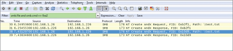
Figure 4-31: Packet list filtered for NT Create calls
You can make one last optimization in the filter. The packet list now shows one line with a filename and the other without a filename in the Info column. This is because the Wireshark SMB dissector doesn't show the filename parameter for a server response. You can inspect the packets again to determine whether the protocol stores this information in a packet. The answer can be found in the flags object, which stores a response variable that you can match against in an expression. You can use the following filter to show only requests going to the server:
smb.file and smb.cmd == 0xa2 and smb.flags.response == 0While the list of files is now human readable, it is neither exportable nor suitable for reporting purposes. TShark is the best tool to get there, combined with some Unix command line magic for the finishing touch. To get a list of all the files accessed, you can run TShark while only showing the SMB filename. This, combined with the filter, results in a list of accessed files, although there will be some duplicates because of the way SMB clients work. To get rid of the duplicates, you can use uniq and sort, both standard Unix tools.
The Unix uniq command will display any unique line but remove subsequent repeated lines. So, if you have “AAA” repeated four times, followed by “BBB” 10 times, then “CCC” another 10 times, then the uniq command will present only “AAA,” “BBB,” and “CCC” once each.
The Unix sort command displays items in a sorted manner, generally alphabetically. For example, let's say you have a list of names, such as “Charlie,” “Alice,” “Dave,” and “Bob.” Using the sort command, the output would be the list in the order: Alice, Bob, Charlie, and Dave.
Try the following command yourself:
tshark -2 -R "smb.file and smb.cmd == 0xa2 and smb.flags.response == 0"
   -T fields -e smb.file -r smb_test.dump \
| sort | uniq -c
You should now have a list of accessed files over SMB without programming one line of code.
This is a glimpse at the power of filters and Wireshark in general. The workflow described in this section is not unique to SMB or this specific case. It can be applied to a lot of protocols by leveraging the excellent bundled dissectors in Wireshark, which support the most popular protocols. By applying this workflow, you can solve a lot of your network-related queries or problems with just filters and some simple elimination.
Packet Colorization
By now you have seen that Wireshark color codes the packets in the Packet List pane. Some people will find this helpful; others will turn it off. It's a personal choice, of course. Before any hasty reaction, let's discuss what's behind the color coding.
Colors are assigned to the packets in one of two ways. The first way packets get colored is defined by the Coloring Rules, a persistent feature of Wireshark. These colors stay as they are configured after Wireshark is shut down or restarted. The second way is temporarily assigning colors to assist for a particular capture. Temporary coloring lasts only for as long as Wireshark is showing that capture. Going forward, we delve into how both of these can be helpful.
Persistent Colors, by Rule
The Coloring Rules, previously called color filters, are persistent, but highly adjustable and scalable. You can view them by clicking the View option on the top menu bar and then selecting Coloring Rules. You get a dialog box like that shown in Figure 4-32. Each rule has a friendly name and has the filter associated with it. Foreground and Background buttons appear near the bottom when any rule is highlighted and enable you to fine-tune the background or font coloring.
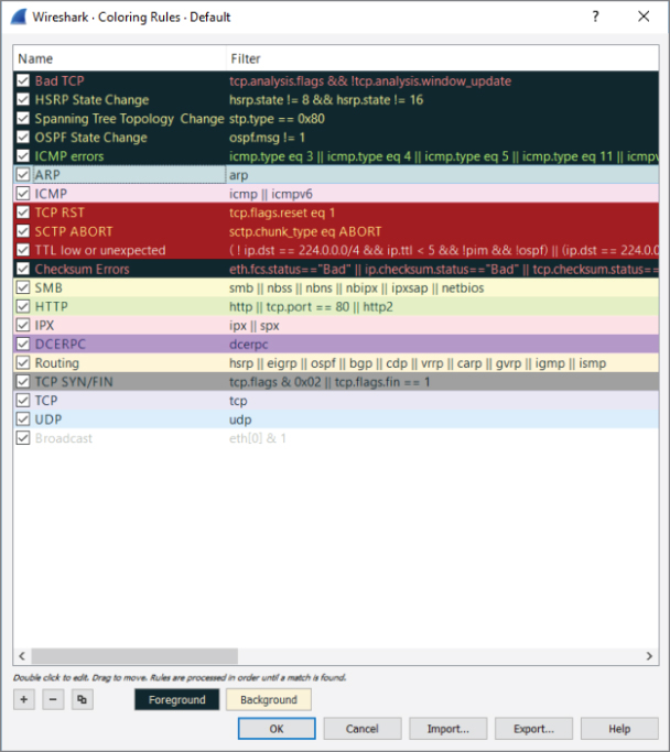
Figure 4-32: Adjusting packet colors
Far more important than adjusting colors, you can adjust the rule condition itself. Double-clicking on a filter allows you to edit and change the reason for coloring a packet.
For example, say you want to adjust the ICMP rule. Right now, the rule colors packets matching this condition:
- icmp || icmpv6
Basically, any ICMP packet, whether IPv4 or IPv6, gets colored that shade of pink. But what if you want to specify ICMP packets coming only from a particular subnet? Then you would adjust the rule to perhaps this:
- icmp || icmpv6 && ip.src==192.168.0.0/16
Now when ping packets originating from the 192.168.0.0 subnet are captured, they will appear in that color. You can use the display filter syntax to adjust any coloring rule.
Temporary Colors, by Choice
The second way packets get colored is by temporarily assigning colors. To colorize an entire conversation (a stream between two or more devices), simply right-click a packet in the Packet List pane and choose Colorize Conversation. As shown in Figure 4-33, you have the option of what layer to distinguish with a color.
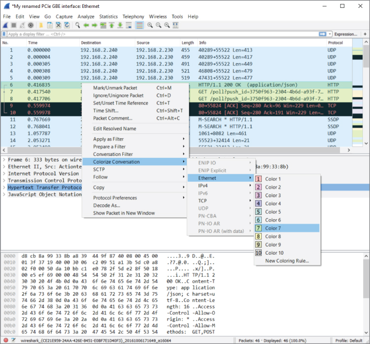
Figure 4-33: Colorizing conversations
In older versions of Wireshark, supported by their documentation, the choice of layer was made for you, coloring “based on TCP first, then UDP, then IP, and at last Ethernet.” The coloring of packets is obviously very flexible. From the GUI and figures, you see how granular a change you can make.
Using Coloring Rules for Troubleshooting
Besides being catchy for the eyes, using colors to distinguish packets can help in troubleshooting. Colorizing the Packet List pane can be revealing, for example, when you are investigating a particular protocol, gauging how often a port appears, or tracing an exchange between devices. When you select and configure your own set of color rules, you also have the option to save your color scheme and even export it for another Wireshark platform or for others to use.
Going further, a collection of color rule sets is available for you to use. On the Wireshark site at the following address, you will find rule sets sent in by Wireshark community members for a wide range of scenarios:
https://wiki.wireshark.org/ColoringRules
Given all the above, we hope to further remove any mystery on why packets appear the way they do in the GUI. Experiment as you like with the two ways of coloring packets you capture or view from other captures.
Viewing Someone Else's Captures
You might find capturing packets at home somewhat predictable. For fun, you browsed a few sites, turned on an extra PC or tablet, and maybe transferred a file or text. It is interesting to watch the SMB, DNS, and DHCP traffic. The next step is capturing traffic while you log into an FTP site—and yes, there's the password in cleartext!
But even after a few experiments like that, your local traffic gets boring. Maybe you want to see protocols that aren't available locally. Or you're curious about malware or some certain malicious packet volley. It's time to find some capture files somewhere else.
You could search using Google, and sure, there are many sources. Instead, let's save the hunting time and offer some of the best sources of pcap files.
First, a repository from a familiar site:
This page includes an exhaustive list of protocol-specific pcap files. If there is any one protocol you want to view, or compare against another, this is your source. It can be very interesting to view the exchange between systems for a number of protocols.
Second, a repository especially appealing for security professionals:
NETRESEC is a software vendor based in Sweden that develops tools for network analysis. With a specialization in network security, it has an impressive set of pcap files you should enjoy parsing through, including those from Capture the Flag events and other competitions, plenty of malware, and forensics traces.
Summary
This chapter has shown a few methods of capturing traffic. To best understand how traffic gets captured, it was first necessary to refresh your understanding about the localhost, its loopback adapter, and what kinds of traffic you can expect to find locally. We captured traffic, both using the GUI and command-line tool TShark.
Beyond the localhost, we covered traffic behavior on the network and how promiscuous mode allows you to see packets beyond your system's needs. You can capture traffic between VMs or across network devices such as hubs and switches. Remembering the key differences between these devices can help answer questions about why you see the traffic you do—or don't.
There was a lot of discussion about when sniffing involves switches. One solution is to create a spanning port, by managing a switch's configuration, to mirror or copy desired traffic to a specific port. Another solution is to use a network tap, which basically replicates network traffic from one or more ports to other ports. Finally, regarding wireless networks, we know that Wireshark can be a challenge. You learned how to enable your own wireless network adapter to view all packets in monitor mode. While a challenge, you can monitor all wireless traffic as well as monitor several WiFi stations, given the right tools and platform.
We discussed the primary supported file formats, explored how to use ring buffers, and divide captures into multiple files. Going the other way, we merged several capture files into one capture file using the command-line tool mergecap. With each capture file handled in Wireshark, the tool adds to a list of recent files opened. We discussed how to better manage that list.
We discussed how Wireshark interprets the packet streams through dissectors. Using the W4SP Lab, we walked through an example of how a dissector can misinterpret a capture—and how to fix it. Lastly, related to dissectors, we discussed in depth how colorization works in the Packet List pane. You can now configure your own rule set as well as share it with others in the community.
Exercises
- Perform two captures, one in promiscuous mode and one not in promiscuous mode. Find any packets only in the trace captured in promiscuous mode. What packet details made you determine how the trace was done?
- Is there a display filter you could have used to rule out the localhost as either a source or destination?
- Find the ARP traffic within the packet dump and ensure the correct dissector is applied to it.
- Design a display filter that will help you see DHCP request and response traffic for when another machine first connects to the network.
- Sniff on a host-only network, a NAT network, and a bridge network.
- Sniff some encrypted WiFi traffic. What do you see?
- Set up your own host-only network using Linux bridging. (Hint: You can use TUN/TAP attached to a Linux bridge, and then bridge the virtual machines to these interfaces.)