Table of Contents for
Grokking Algorithms: An illustrated guide for programmers and other curious people
 Grokking Algorithms: An illustrated guide for programmers and other curious people
Published by
Manning Publications, 2016
Grokking Algorithms: An illustrated guide for programmers and other curious people
Published by
Manning Publications, 2016
- Cover
- Grokking Algorithms: An illustrated guide for programmers and other curious people
- Copyright
- Brief Table of Contents
- Table of Contents
- Preface
- Acknowledgments
- About this Book
- Chapter 1. Introduction to Algorithms
- Chapter 2. Selection Sort
- Chapter 3. Recursion
- Chapter 4. Quicksort
- Chapter 5. Hash Tables
- Chapter 6. Breadth-first Search
- Chapter 7. Dijkstra’s algorithm
- Chapter 8. Greedy algorithms
- Chapter 9. Dynamic programming
- Chapter 10. K-nearest neighbors
- Chapter 11. Where to go next
- Appendix. Answers to Exercises
- Index
Chapter 8. Greedy algorithms

- You learn how to tackle the impossible: problems that have no fast algorithmic solution (NP-complete problems).
- You learn how to identify such problems when you see them, so you don’t waste time trying to find a fast algorithm for them.
- You learn about approximation algorithms, which you can use to find an approximate solution to an NP-complete problem quickly.
- You learn about the greedy strategy, a very simple problem-solving strategy.
The classroom scheduling problem

Suppose you have a classroom and want to hold as many classes here as possible. You get a list of classes.
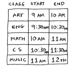
You can’t hold all of these classes in there, because some of them overlap.
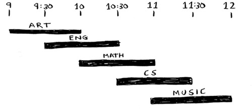
You want to hold as many classes as possible in this classroom. How do you pick what set of classes to hold, so that you get the biggest set of classes possible?
Sounds like a hard problem, right? Actually, the algorithm is so easy, it might surprise you. Here’s how it works:
- Pick the class that ends the soonest. This is the first class you’ll hold in this classroom.
- Now, you have to pick a class that starts after the first class. Again, pick the class that ends the soonest. This is the second class you’ll hold.
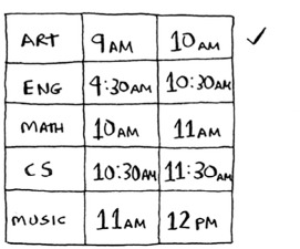
Keep doing this, and you’ll end up with the answer! Let’s try it out. Art ends the soonest, at 10:00 a.m., so that’s one of the classes you pick.
Now you need the next class that starts after 10:00 a.m. and ends the soonest.
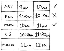
English is out because it conflicts with Art, but Math works.
Finally, CS conflicts with Math, but Music works.
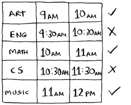
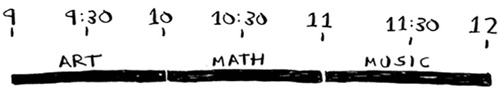
So these are the three classes you’ll hold in this classroom.
A lot of people tell me that this algorithm seems easy. It’s too obvious, so it must be wrong. But that’s the beauty of greedy algorithms: they’re easy! A greedy algorithm is simple: at each step, pick the optimal move. In this case, each time you pick a class, you pick the class that ends the soonest. In technical terms: at each step you pick the locally optimal solution, and in the end you’re left with the globally optimal solution. Believe it or not, this simple algorithm finds the optimal solution to this scheduling problem!
Obviously, greedy algorithms don’t always work. But they’re simple to write! Let’s look at another example.
The knapsack problem

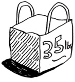
Suppose you’re a greedy thief. You’re in a store with a knapsack, and there are all these items you can steal. But you can only take what you can fit in your knapsack. The knapsack can hold 35 pounds.
You’re trying to maximize the value of the items you put in your knapsack. What algorithm do you use?
Again, the greedy strategy is pretty simple:
- Pick the most expensive thing that will fit in your knapsack.
- Pick the next most expensive thing that will fit in your knapsack. And so on.
Except this time, it doesn’t work! For example, suppose there are three items you can steal.

Your knapsack can hold 35 pounds of items. The stereo system is the most expensive, so you steal that. Now you don’t have space for anything else.
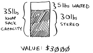
You got $3,000 worth of goods. But wait! If you’d picked the laptop and the guitar instead, you could have had $3,500 worth of loot!

Clearly, the greedy strategy doesn’t give you the optimal solution here. But it gets you pretty close. In the next chapter, I’ll explain how to calculate the correct solution. But if you’re a thief in a shopping center, you don’t care about perfect. “Pretty good” is good enough.
Here’s the takeaway from this second example: sometimes, perfect is the enemy of good. Sometimes all you need is an algorithm that solves the problem pretty well. And that’s where greedy algorithms shine, because they’re simple to write and usually get pretty close.
Exercises
You work for a furniture company, and you have to ship furniture all over the country. You need to pack your truck with boxes. All the boxes are of different sizes, and you’re trying to maximize the space you use in each truck. How would you pick boxes to maximize space? Come up with a greedy strategy. Will that give you the optimal solution?
You’re going to Europe, and you have seven days to see everything you can. You assign a point value to each item (how much you want to see it) and estimate how long it takes. How can you maximize the point total (seeing all the things you really want to see) during your stay? Come up with a greedy strategy. Will that give you the optimal solution?
Let’s look at one last example. This is an example where greedy algorithms are absolutely necessary.
The set-covering problem
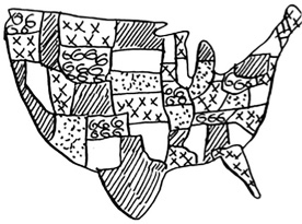
Suppose you’re starting a radio show. You want to reach listeners in all 50 states. You have to decide what stations to play on to reach all those listeners. It costs money to be on each station, so you’re trying to minimize the number of stations you play on. You have a list of stations.
Each station covers a region, and there’s overlap.
How do you figure out the smallest set of stations you can play on to cover all 50 states? Sounds easy, doesn’t it? Turns out it’s extremely hard. Here’s how to do it:
- List every possible subset of stations. This is called the power set. There are 2^n possible subsets.
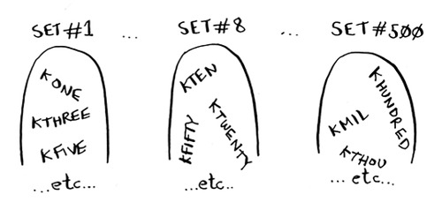
- From these, pick the set with the smallest number of stations that covers all 50 states.
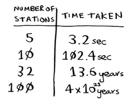
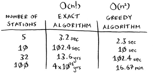
The problem is, it takes a long time to calculate every possible subset of stations. It takes O(2^n) time, because there are 2^n stations. It’s possible to do if you have a small set of 5 to 10 stations. But with all the examples here, think about what will happen if you have a lot of items. It takes much longer if you have more stations. Suppose you can calculate 10 subsets per second.
There’s no algorithm that solves it fast enough! What can you do?
Approximation algorithms
Greedy algorithms to the rescue! Here’s a greedy algorithm that comes pretty close:
- Pick the station that covers the most states that haven’t been covered yet. It’s OK if the station covers some states that have been covered already.
- Repeat until all the states are covered.
This is called an approximation algorithm. When calculating the exact solution will take too much time, an approximation algorithm will work. Approximation algorithms are judged by
- How fast they are
- How close they are to the optimal solution
Greedy algorithms are a good choice because not only are they simple to come up with, but that simplicity means they usually run fast, too. In this case, the greedy algorithm runs in O(n^2) time, where n is the number of radio stations.
Let’s see how this problem looks in code.
Code for setup
For this example, I’m going to use a subset of the states and the stations to keep things simple.
First, make a list of the states you want to cover:

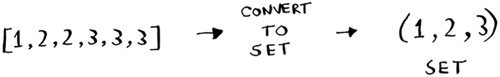
I used a set for this. A set is like a list, except that each item can show up only once in a set. Sets can’t have duplicates. For example, suppose you had this list:
>>> arr = [1, 2, 2, 3, 3, 3]
And you converted it to a set:
>>> set(arr)
set([1, 2, 3])
1, 2, and 3 all show up just once in a set.
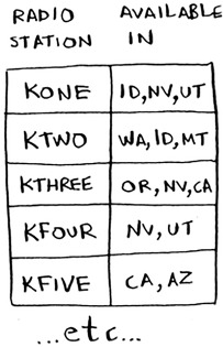
You also need the list of stations that you’re choosing from. I chose to use a hash for this:
stations = {}
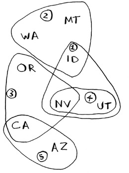
stations["kone"] = set(["id", "nv", "ut"])
stations["ktwo"] = set(["wa", "id", "mt"])
stations["kthree"] = set(["or", "nv", "ca"])
stations["kfour"] = set(["nv", "ut"])
stations["kfive"] = set(["ca", "az"])
The keys are station names, and the values are the states they cover. So in this example, the kone station covers Idaho, Nevada, and Utah. All the values are sets, too. Making everything a set will make your life easier, as you’ll see soon.
Finally, you need something to hold the final set of stations you’ll use:
final_stations = set()
Calculating the answer
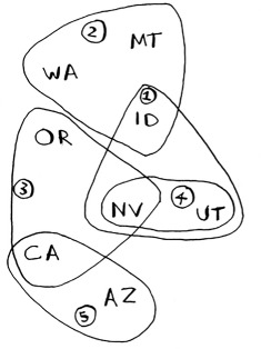
Now you need to calculate what stations you’ll use. Take a look at the image at right, and see if you can predict what stations you should use.
There can be more than one correct solution. You need to go through every station and pick the one that covers the most uncovered states. I’ll call this best_station:
best_station = None
states_covered = set()
for station, states_for_station in stations.items():
states_covered is a set of all the states this station covers that haven’t been covered yet. The for loop allows you to loop over every station to see which one is the best station. Let’s look at the body of the for loop:
There’s a funny-looking line here:
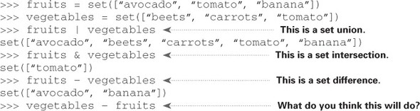
covered = states_needed & states_for_station
What’s going on?
Sets
Suppose you have a set of fruits.

You also have a set of vegetables.

When you have two sets, you can do some fun things with them.
Here are some things you can do with sets.
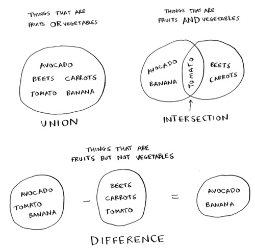
- A set union means “combine both sets.”
- A set intersection means “find the items that show up in both sets” (in this case, just the tomato).
- A set difference means “subtract the items in one set from the items in the other set.”
For example:
- Sets are like lists, except sets can’t have duplicates.
- You can do some interesting operations on sets, like union, intersection, and difference.
Back to the code
Let’s get back to the original example.
This is a set intersection:
covered = states_needed & states_for_station
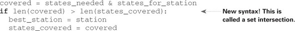
covered is a set of states that were in both states_needed and states_for_station. So covered is the set of uncovered states that this station covers! Next you check whether this station covers more states than the current best_station:
if len(covered) > len(states_covered):
  best_station = station
  states_covered = covered

If so, this station is the new best_station. Finally, after the for loop is over, you add best_station to the final list of stations:
final_stations.add(best_station)
You also need to update states_needed. Because this station covers some states, those states aren’t needed anymore:
states_needed -= states_covered
And you loop until states_needed is empty. Here’s the full code for the loop:
while states_needed:
  best_station = None
  states_covered = set()
  for station, states in stations.items():
    covered = states_needed & states
    if len(covered) > len(states_covered):
     best_station = station
     states_covered = covered

states_needed -= states_covered
final_stations.add(best_station)
Finally, you can print final_stations, and you should see this:
>>> print final_stations
set(['ktwo', 'kthree', 'kone', 'kfive'])
Is that what you expected? Instead of stations 1, 2, 3, and 5, you could have chosen stations 2, 3, 4, and 5. Let’s compare the run time of the greedy algorithm to the exact algorithm.
Exercises
For each of these algorithms, say whether it’s a greedy algorithm or not.
Quicksort
Breadth-first search
Dijkstra’s algorithm
NP-complete problems
To solve the set-covering problem, you had to calculate every possible set.

Maybe you were reminded of the traveling salesperson problem from chapter 1. In this problem, a salesperson has to visit five different cities.
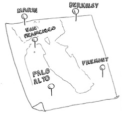
And he’s trying to figure out the shortest route that will take him to all five cities. To find the shortest route, you first have to calculate every possible route.
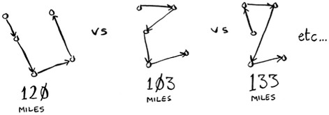
How many routes do you have to calculate for five cities?
Traveling salesperson, step by step
Let’s start small. Suppose you only have two cities. There are two routes to choose from.
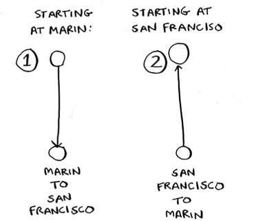
You may think this should be the same route. After all, isn’t SF > Marin the same distance as Marin > SF? Not necessarily. Some cities (like San Francisco) have a lot of one-way streets, so you can’t go back the way you came. You might also have to go 1 or 2 miles out of the way to find an on-ramp to a highway. So these two routes aren’t necessarily the same.
You may be wondering, “In the traveling salesperson problem, is there a specific city you need to start from?” For example, let’s say I’m the traveling salesperson. I live in San Francisco, and I need to go to four other cities. San Francisco would be my start city.
But sometimes the start city isn’t set. Suppose you’re FedEx, trying to deliver a package to the Bay Area. The package is being flown in from Chicago to one of 50 FedEx locations in the Bay Area. Then that package will go on a truck that will travel to different locations delivering packages. Which location should it get flown to? Here the start location is unknown. It’s up to you to compute the optimal path and start location for the traveling salesperson.
The running time for both versions is the same. But it’s an easier example if there’s no defined start city, so I’ll go with that version.
Two cities = two possible routes.
3 cities
Now suppose you add one more city. How many possible routes are there?
If you start at Berkeley, you have two more cities to visit.
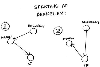
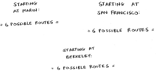
There are six total routes, two for each city you can start at.
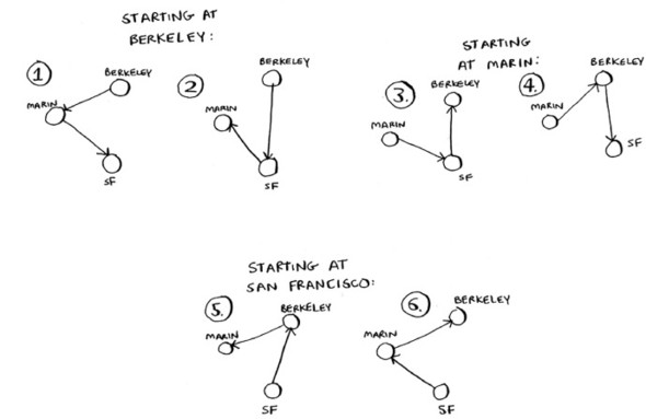
So three cities = six possible routes.
4 cities
Let’s add another city, Fremont. Now suppose you start at Fremont.
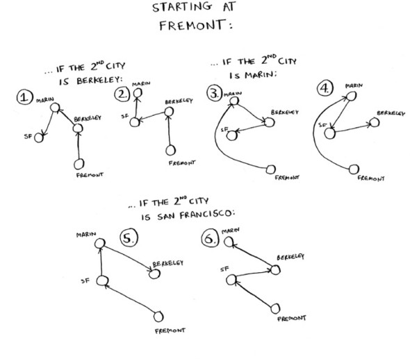
There are six possible routes starting from Fremont. And hey! They look a lot like the six routes you calculated earlier, when you had only three cities. Except now all the routes have an additional city, Fremont! There’s a pattern here. Suppose you have four cities, and you pick a start city, Fremont. There are three cities left. And you know that if there are three cities, there are six different routes for getting between those cities. If you start at Fremont, there are six possible routes. You could also start at one of the other cities.
Four possible start cities, with six possible routes for each start city = 4 * 6 = 24 possible routes.
Do you see a pattern? Every time you add a new city, you’re increasing the number of routes you have to calculate.
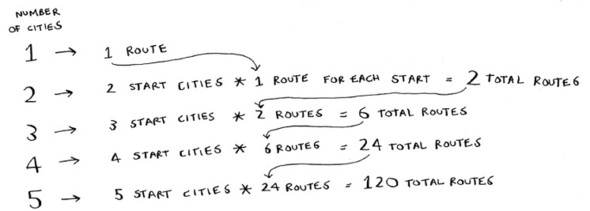
How many possible routes are there for six cities? If you guessed 720, you’re right. 5,040 for 7 cities, 40,320 for 8 cities.
This is called the factorial function (remember reading about this in chapter 3?). So 5! = 120. Suppose you have 10 cities. How many possible routes are there? 10! = 3,628,800. You have to calculate over 3 million possible routes for 10 cities. As you can see, the number of possible routes becomes big very fast! This is why it’s impossible to compute the “correct” solution for the traveling-salesperson problem if you have a large number of cities.
The traveling-salesperson problem and the set-covering problem both have something in common: you calculate every possible solution and pick the smallest/shortest one. Both of these problems are NP-complete.
What’s a good approximation algorithm for the traveling salesperson? Something simple that finds a short path. See if you can come up with an answer before reading on.
Here’s how I would do it: arbitrarily pick a start city. Then, each time the salesperson has to pick the next city to visit, they pick the closest unvisited city. Suppose they start in Marin.
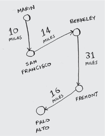
Total distance: 71 miles. Maybe it’s not the shortest path, but it’s still pretty short.
Here’s the short explanation of NP-completeness: some problems are famously hard to solve. The traveling salesperson and the set-covering problem are two examples. A lot of smart people think that it’s not possible to write an algorithm that will solve these problems quickly.
How do you tell if a problem is NP-complete?
Jonah is picking players for his fantasy football team. He has a list of abilities he wants: good quarterback, good running back, good in rain, good under pressure, and so on. He has a list of players, where each player fulfills some abilities.

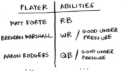
Jonah needs a team that fulfills all his abilities, and the team size is limited. “Wait a second,” Jonah realizes. “This is a set-covering problem!”
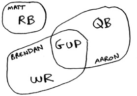
Jonah can use the same approximation algorithm to create his team:
- Find the player who fulfills the most abilities that haven’t been fulfilled yet.
- Repeat until the team fulfills all abilities (or you run out of space on the team).
NP-complete problems show up everywhere! It’s nice to know if the problem you’re trying to solve is NP-complete. At that point, you can stop trying to solve it perfectly, and solve it using an approximation algorithm instead. But it’s hard to tell if a problem you’re working on is NP-complete. Usually there’s a very small difference between a problem that’s easy to solve and an NP-complete problem. For example, in the previous chapters, I talked a lot about shortest paths. You know how to calculate the shortest way to get from point A to point B.
But if you want to find the shortest path that connects several points, that’s the traveling-salesperson problem, which is NP-complete. The short answer: there’s no easy way to tell if the problem you’re working on is NP-complete. Here are some giveaways:
- Your algorithm runs quickly with a handful of items but really slows down with more items.
- “All combinations of X” usually point to an NP-complete problem.
- Do you have to calculate “every possible version” of X because you can’t break it down into smaller sub-problems? Might be NP-complete.
- If your problem involves a sequence (such as a sequence of cities, like traveling salesperson), and it’s hard to solve, it might be NP-complete.
- If your problem involves a set (like a set of radio stations) and it’s hard to solve, it might be NP-complete.
- Can you restate your problem as the set-covering problem or the traveling-salesperson problem? Then your problem is definitely NP-complete.
Exercises
A postman needs to deliver to 20 homes. He needs to find the shortest route that goes to all 20 homes. Is this an NP-complete problem?
Finding the largest clique in a set of people (a clique is a set of people who all know each other). Is this an NP-complete problem?
You’re making a map of the USA, and you need to color adjacent states with different colors. You have to find the minimum number of colors you need so that no two adjacent states are the same color. Is this an NP-complete problem?
Recap
- Greedy algorithms optimize locally, hoping to end up with a global optimum.
- NP-complete problems have no known fast solution.
- If you have an NP-complete problem, your best bet is to use an approximation algorithm.
- Greedy algorithms are easy to write and fast to run, so they make good approximation algorithms.