Table of Contents for
Introduction to Machine Learning with Python
 Introduction to Machine Learning with Python
Published by
O'Reilly Media, Inc., 2016
Introduction to Machine Learning with Python
Published by
O'Reilly Media, Inc., 2016
- Cover
- nav
- Introduction to Machine Learning with Python
- Introduction to Machine Learning with Python
- Preface
- 1. Introduction
- 2. Supervised Learning
- 3. Unsupervised Learning and Preprocessing
- 4. Representing Data and Engineering Features
- 5. Model Evaluation and Improvement
- 6. Algorithm Chains and Pipelines
- 7. Working with Text Data
- 8. Wrapping Up
- Index
- About the Authors
- Colophon
Chapter 5. Model Evaluation and Improvement
Having discussed the fundamentals of supervised and unsupervised learning, and having explored a variety of machine learning algorithms, we will now dive more deeply into evaluating models and selecting parameters.
We will focus on the supervised methods, regression and classification, as evaluating and selecting models in unsupervised learning is often a very qualitative process (as we saw in Chapter 3).
To evaluate our supervised models, so far we have split our dataset into
a training set and a test set using the train_test_split function,
built a model on the training set by calling the fit method, and
evaluated it on the test set using the score method, which for
classification computes the fraction of correctly classified samples.
Here’s an example of that process:
In[1]:
fromsklearn.datasetsimportmake_blobsfromsklearn.linear_modelimportLogisticRegressionfromsklearn.model_selectionimporttrain_test_split# create a synthetic datasetX,y=make_blobs(random_state=0)# split data and labels into a training and a test setX_train,X_test,y_train,y_test=train_test_split(X,y,random_state=0)# instantiate a model and fit it to the training setlogreg=LogisticRegression().fit(X_train,y_train)# evaluate the model on the test set("Test set score: {:.2f}".format(logreg.score(X_test,y_test)))
Out[1]:
Test set score: 0.88
Remember, the reason we split our data into training and test sets is that we are interested in measuring how well our model generalizes to new, previously unseen data. We are not interested in how well our model fit the training set, but rather in how well it can make predictions for data that was not observed during training.
In this chapter, we will expand on two aspects of this evaluation. We
will first introduce cross-validation, a more robust way to assess
generalization performance, and discuss methods to evaluate
classification and regression performance that go beyond the default
measures of accuracy and R2 provided by the score
method.
We will also discuss grid search, an effective method for adjusting the parameters in supervised models for the best generalization performance.
5.1 Cross-Validation
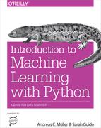
Cross-validation is a statistical method of evaluating generalization performance that is more stable and thorough than using a split into a training and a test set. In cross-validation, the data is instead split repeatedly and multiple models are trained. The most commonly used version of cross-validation is k-fold cross-validation, where k is a user-specified number, usually 5 or 10. When performing five-fold cross-validation, the data is first partitioned into five parts of (approximately) equal size, called folds. Next, a sequence of models is trained. The first model is trained using the first fold as the test set, and the remaining folds (2–5) are used as the training set. The model is built using the data in folds 2–5, and then the accuracy is evaluated on fold 1. Then another model is built, this time using fold 2 as the test set and the data in folds 1, 3, 4, and 5 as the training set. This process is repeated using folds 3, 4, and 5 as test sets. For each of these five splits of the data into training and test sets, we compute the accuracy. In the end, we have collected five accuracy values. The process is illustrated in Figure 5-1:
In[2]:
mglearn.plots.plot_cross_validation()
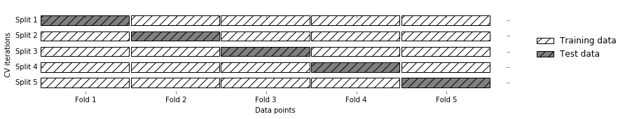
Figure 5-1. Data splitting in five-fold cross-validation
Usually, the first fifth of the data is the first fold, the second fifth of the data is the second fold, and so on.
5.1.1 Cross-Validation in scikit-learn
Cross-validation is implemented in scikit-learn using the
cross_val_score function from the model_selection module. The
parameters of the cross_val_score function are the model we want to
evaluate, the training data, and the ground-truth labels. Let’s evaluate
LogisticRegression on the iris dataset:
In[3]:
fromsklearn.model_selectionimportcross_val_scorefromsklearn.datasetsimportload_irisfromsklearn.linear_modelimportLogisticRegressioniris=load_iris()logreg=LogisticRegression()scores=cross_val_score(logreg,iris.data,iris.target)("Cross-validation scores: {}".format(scores))
Out[3]:
Cross-validation scores: [0.961 0.922 0.958]
Here, cross_val_score performed three-fold cross-validation and
therefore returned three scores. By default, cross_val_score performs
three-fold cross-validation in earlier versions of scikit-learn, and
will perform five-fold cross-validation by default (starting with
scikit-learn 0.22). We can change the number of folds used by changing
the cv parameter:
In[4]:
scores=cross_val_score(logreg,iris.data,iris.target,cv=5)("Cross-validation scores: {}".format(scores))
Out[4]:
Cross-validation scores: [1. 0.967 0.933 0.9 1. ]
It’s recommended to use at least five-fold cross-validation. A common way to summarize the cross-validation accuracy is to compute the mean:
In[5]:
("Average cross-validation score: {:.2f}".format(scores.mean()))
Out[5]:
Average cross-validation score: 0.96
Using the mean cross-validation we can conclude that we expect the model
to be around 96% accurate on average. Looking at all five scores
produced by the five-fold cross-validation, we can also conclude that
there is a relatively high variance in the accuracy between folds,
ranging from 100% accuracy to 90% accuracy. This could imply that the
model is very dependent on the particular folds used for training, but
it could also just be a consequence of the small size of the dataset.
There is a second function you can use for cross-validation, called
cross_validate. It has a similar interface to cross_val_score, but
returns a dictionary containing training and test times (and optionally
the training score, in addition to the test scores) for each split:
In[6]:
fromsklearn.model_selectionimportcross_validateres=cross_validate(logreg,iris.data,iris.target,cv=5,return_train_score=True)display(res)
Out[6]:
{'fit_time': array([0.002, 0.002, 0.002, 0.001, 0.002]),
 'score_time': array([0.   , 0.   , 0.001, 0.001, 0.001]),
 'test_score': array([1.   , 0.967, 0.933, 0.9  , 1.   ]),
 'train_score': array([0.95 , 0.967, 0.967, 0.975, 0.958])}
Using pandas, we can nicely display these results and compute summaries:
In[7]:
res_df=pd.DataFrame(res)display(res_df)("Mean times and scores:\n",res_df.mean())
Out[7]:
[cols=",,,,",options="header",]
|===============================================
| |fit_time |score_time |test_score |train_score
|0 |1.50e-03 |4.62e-04 |1.00 |0.95
|1 |1.58e-03 |4.99e-04 |0.97 |0.97
|2 |1.60e-03 |6.45e-04 |0.93 |0.97
|3 |1.49e-03 |5.19e-04 |0.90 |0.97
|4 |1.54e-03 |1.06e-03 |1.00 |0.96
|===============================================

Mean times and scores:
 fit_time       1.54e-03
score_time     6.37e-04
test_score     9.60e-01
train_score    9.63e-01
dtype: float64
5.1.2 Benefits of Cross-Validation
There are several benefits to using cross-validation instead of a single
split into a training and a test set. First, remember that
train_test_split performs a random split of the data. Imagine that we
are “lucky” when randomly splitting the data, and all examples that are
hard to classify end up in the training set. In that case, the test set
will only contain “easy” examples, and our test set accuracy will be
unrealistically high. Conversely, if we are “unlucky,” we might have
randomly put all the hard-to-classify examples in the test set and
consequently obtain an unrealistically low score. However, when using
cross-validation, each example will be in the test set exactly once:
each example is in one of the folds, and each fold is the test set once.
Therefore, the model needs to generalize well to all of the samples in
the dataset for all of the cross-validation scores (and their mean) to
be high.
Having multiple splits of the data also provides some information about
how sensitive our model is to the selection of the training dataset.
For the iris dataset, we saw accuracies
between 90% and 100%. This is quite a range, and it provides us with an
idea about how the model might perform in the worst case and best
case scenarios when applied to new data.
Another benefit of cross-validation as compared to using a single split
of the data is that we use our data more effectively. When using
train_test_split, we usually use 75% of the data for training and 25%
of the data for evaluation. When using five-fold cross-validation, in
each iteration we can use four-fifths of the data (80%) to fit the model. When
using 10-fold cross-validation, we can use nine-tenths of the data (90%) to
fit the model. More data will usually result in more accurate models.
The main disadvantage of cross-validation is increased computational cost. As we are now training k models instead of a single model, cross-validation will be roughly k times slower than doing a single split of the data.
Tip
It is important to keep in mind that cross-validation is not
a way to build a model that can be applied to new data. Cross-validation
does not return a model. When calling cross_val_score, multiple models
are built internally, but the purpose of cross-validation is only to
evaluate how well a given algorithm will generalize when trained on a
specific dataset.
5.1.3 Stratified k-Fold Cross-Validation and Other Strategies
Splitting the dataset into k folds by starting with the first one-k-th
part of the data, as described in the previous section, might not always be a good idea. For
example, let’s have a look at the iris dataset:
In[8]:
fromsklearn.datasetsimportload_irisiris=load_iris()("Iris labels:\n{}".format(iris.target))
Out[8]:
Iris labels:
[0 0 0 0 0 0 0 0 0 0 0 0 0 0 0 0 0 0 0 0 0 0 0 0 0 0 0 0 0 0 0 0 0 0 0 0 0
 0 0 0 0 0 0 0 0 0 0 0 0 0 1 1 1 1 1 1 1 1 1 1 1 1 1 1 1 1 1 1 1 1 1 1 1 1
 1 1 1 1 1 1 1 1 1 1 1 1 1 1 1 1 1 1 1 1 1 1 1 1 1 1 2 2 2 2 2 2 2 2 2 2 2
 2 2 2 2 2 2 2 2 2 2 2 2 2 2 2 2 2 2 2 2 2 2 2 2 2 2 2 2 2 2 2 2 2 2 2 2 2
 2 2]
As you can see, the first third of the data is the class 0, the second
third is the class 1, and the last third is the class 2. Imagine doing
three-fold cross-validation on this dataset. The first fold would be
only class 0, so in the first split of the data, the test set would be
only class 0, and the training set would be only classes 1 and 2. As
the classes in training and test sets would be different for all three
splits, the three-fold cross-validation accuracy would be zero on this
dataset. That is not very helpful, as we can do much better than 0%
accuracy on iris.
As the simple k-fold strategy fails here, scikit-learn does not use
it for classification, but rather uses stratified k-fold
cross-validation. In stratified cross-validation, we split the data
such that the proportions between classes are the same in each fold as
they are in the whole dataset, as illustrated in
Figure 5-2:
In[9]:
mglearn.plots.plot_stratified_cross_validation()
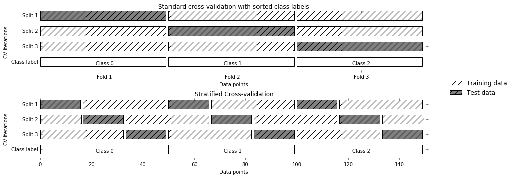
Figure 5-2. Comparison of standard cross-validation and stratified cross-validation when the data is ordered by class label
For example, if 90% of your samples belong to class A and 10% of your samples belong to class B, then stratified cross-validation ensures that in each fold, 90% of samples belong to class A and 10% of samples belong to class B.
It is usually a good idea to use stratified k-fold cross-validation instead of k-fold cross-validation to evaluate a classifier, because it results in more reliable estimates of generalization performance. In the case of only 10% of samples belonging to class B, using standard k-fold cross-validation it might easily happen that one fold only contains samples of class A. Using this fold as a test set would not be very informative about the overall performance of the classifier.
For regression, scikit-learn uses the standard k-fold cross-validation
by default. It would be possible to also try to make each fold
representative of the different values the regression target has, but
this is not a commonly used strategy and would be surprising to most
users.
More control over cross-validation
We saw earlier that we can adjust the number of folds that are used in
cross_val_score using the cv parameter. However, scikit-learn allows
for much finer control over what happens during the splitting of the
data by providing a cross-validation splitter as the cv parameter.
For most use cases, the defaults of k-fold cross-validation for
regression and stratified k-fold for classification work well, but there
are some cases where you might want to use a different strategy. Say, for
example, we want to use the standard k-fold cross-validation on a
classification dataset to reproduce someone else’s results. To do this,
we first have to import the KFold splitter class from the
model_selection module and instantiate it with the number of folds
we want to use:
In[10]:
fromsklearn.model_selectionimportKFoldkfold=KFold(n_splits=5)
Then, we can pass the kfold splitter object as the cv parameter to
cross_val_score:
In[11]:
("Cross-validation scores:\n{}".format(cross_val_score(logreg,iris.data,iris.target,cv=kfold)))
Out[11]:
Cross-validation scores:
[1.    0.933 0.433 0.967 0.433]
This way, we can verify that it is indeed a really bad idea to use
three-fold (nonstratified) cross-validation on the iris dataset:
In[12]:
kfold=KFold(n_splits=3)("Cross-validation scores:\n{}".format(cross_val_score(logreg,iris.data,iris.target,cv=kfold)))
Out[12]:
Cross-validation scores:
[0. 0. 0.]
Remember: each fold corresponds to one of the classes in the iris
dataset, and so nothing can be learned. Another way to resolve this
problem is to shuffle the data instead of stratifying the folds, to
remove the ordering of the samples by label. We can do that by setting the
shuffle parameter of KFold to True. If we shuffle the data, we
also need to fix the random_state to get a reproducible shuffling.
Otherwise, each run of cross_val_score would yield a different result,
as each time a different split would be used (this might not be a
problem, but can be surprising). Shuffling the data before splitting it yields a much better result:
In[13]:
kfold=KFold(n_splits=3,shuffle=True,random_state=0)("Cross-validation scores:\n{}".format(cross_val_score(logreg,iris.data,iris.target,cv=kfold)))
Out[13]:
Cross-validation scores:
[0.9  0.96 0.96]
Leave-one-out cross-validation
Another frequently used cross-validation method is leave-one-out. You can think of leave-one-out cross-validation as k-fold cross-validation where each fold is a single sample. For each split, you pick a single data point to be the test set. This can be very time consuming, particularly for large datasets, but sometimes provides better estimates on small datasets:
In[14]:
fromsklearn.model_selectionimportLeaveOneOutloo=LeaveOneOut()scores=cross_val_score(logreg,iris.data,iris.target,cv=loo)("Number of cv iterations: ",len(scores))("Mean accuracy: {:.2f}".format(scores.mean()))
Out[14]:
Number of cv iterations:  150
Mean accuracy: 0.95
Shuffle-split cross-validation
Another, very flexible strategy for cross-validation is shuffle-split
cross-validation. In shuffle-split cross-validation, each split samples
train_size many points for the training set and test_size many
(disjoint) point for the test set. This splitting is repeated n_splits
times. Figure 5-3 illustrates running four iterations of
splitting a dataset consisting of 10 points, with a training set of 5
points and test sets of 2 points each (you can use integers for
train_size and test_size to use absolute sizes for these sets, or
floating-point numbers to use fractions of the whole dataset):
In[15]:
mglearn.plots.plot_shuffle_split()
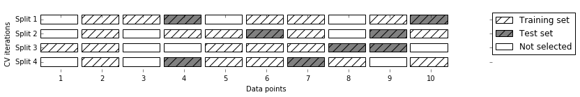
Figure 5-3. ShuffleSplit with 10 points, train_size=5, test_size=2, and n_splits=4
The following code splits the dataset into 50% training set and 50% test set for 10 iterations:
In[16]:
fromsklearn.model_selectionimportShuffleSplitshuffle_split=ShuffleSplit(test_size=.5,train_size=.5,n_splits=10)scores=cross_val_score(logreg,iris.data,iris.target,cv=shuffle_split)("Cross-validation scores:\n{}".format(scores))
Out[16]:
Cross-validation scores:
[0.973 0.92  0.96  0.96  0.893 0.947 0.88  0.893 0.947 0.947]
Shuffle-split cross-validation allows for control over the number of
iterations independently of the training and test sizes, which can
sometimes be helpful. It also allows for using only part of the data in
each iteration, by providing train_size and test_size settings that
don’t add up to one. Subsampling the data in this way can be useful for
experimenting with large datasets.
There is also a stratified variant of
ShuffleSplit, aptly named StratifiedShuffleSplit, which can provide
more reliable results for classification tasks.
Cross-validation with groups
Another very common setting for cross-validation is when there are groups in the data that are highly related. Say you want to build a system to recognize emotions from pictures of faces, and you collect a dataset of pictures of 100 people where each person is captured multiple times, showing various emotions. The goal is to build a classifier that can correctly identify emotions of people not in the dataset. You could use the default stratified cross-validation to measure the performance of a classifier here. However, it is likely that pictures of the same person will be in both the training and the test set. It will be much easier for a classifier to detect emotions in a face that is part of the training set, compared to a completely new face. To accurately evaluate the generalization to new faces, we must therefore ensure that the training and test sets contain images of different people.
To achieve this, we can use GroupKFold, which takes an array of groups
as argument that we can use to indicate which person is in the image. The groups array here indicates groups in the data that should not be split when
creating the training and test sets, and should not be confused with the
class label.
This example of groups in the data is common in medical applications, where you might have multiple samples from the same patient, but are interested in generalizing to new patients. Similarly, in speech recognition, you might have multiple recordings of the same speaker in your dataset, but are interested in recognizing speech of new speakers.
The following is an example of using a synthetic dataset with a grouping given
by the groups array. The dataset consists of 12 data points, and for
each of the data points, groups specifies which group (think patient)
the point belongs to. The groups specify that there are four groups, and the
first three samples belong to the first group, the next four samples
belong to the second group, and so on:
In[17]:
fromsklearn.model_selectionimportGroupKFold# create synthetic datasetX,y=make_blobs(n_samples=12,random_state=0)# assume the first three samples belong to the same group,# then the next four, etc.groups=[0,0,0,1,1,1,1,2,2,3,3,3]scores=cross_val_score(logreg,X,y,groups,cv=GroupKFold(n_splits=3))("Cross-validation scores:\n{}".format(scores))
Out[17]:
Cross-validation scores:
[0.75  0.8   0.667]
The samples don’t need to be ordered by group; we just did this for illustration purposes. The splits that are calculated based on these labels are visualized in Figure 5-4. As you can see, for each split, each group is either entirely in the training set or entirely in the test set:
In[18]:
mglearn.plots.plot_group_kfold()
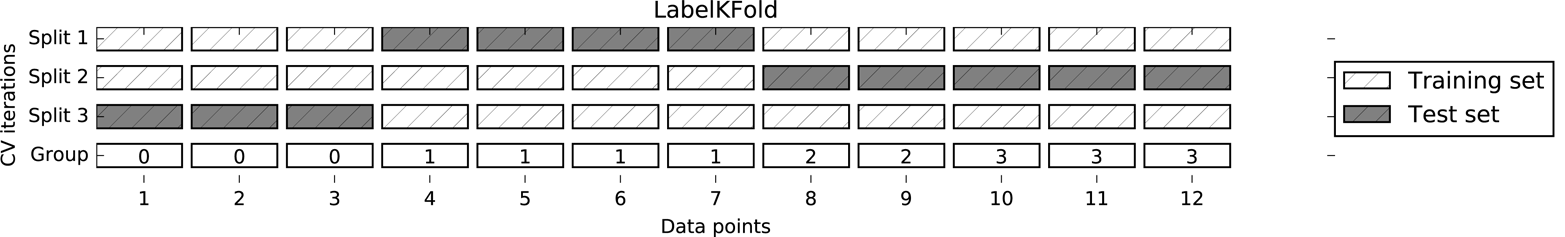
Figure 5-4. Label-dependent splitting with GroupKFold
There are more splitting strategies for cross-validation in
scikit-learn, which allow for an even greater variety of use cases (you can find these in the scikit-learn user guide). However, the standard KFold,
StratifiedKFold, and GroupKFold are by far the most commonly used
ones.
5.2 Grid Search
Now that we know how to evaluate how well a model generalizes, we can
take the next step and improve the model’s generalization performance by
tuning its parameters. We discussed the parameter settings of many of
the algorithms in scikit-learn in Chapters 2 and 3, and it is important
to understand what the parameters mean before trying to adjust them.
Finding the values of the important parameters of a model (the ones that
provide the best generalization performance) is a tricky task, but
necessary for almost all models and datasets. Because it is such a
common task, there are standard methods in scikit-learn to help you with
it. The most commonly used method is grid search, which basically
means trying all possible combinations of the parameters of interest.
Consider the case of a kernel SVM with an RBF (radial basis function)
kernel, as implemented in the SVC class. As we discussed in Chapter 2,
there are two important parameters: the kernel bandwidth, gamma, and the
regularization parameter, C. Say we want to try the values
0.001, 0.01, 0.1, 1, 10, and 100 for the parameter C, and the same for
gamma. Because we have six different settings for C and gamma that
we want to try, we have 36 combinations of parameters in total. Looking
at all possible combinations creates a table (or grid) of parameter
settings for the SVM, as shown here:
| C = 0.001 | C = 0.01 | … | C = 10 | ||
|---|---|---|---|---|---|
gamma=0.001 |
SVC(C=0.001, gamma=0.001) |
SVC(C=0.01, gamma=0.001) |
… |
SVC(C=10, gamma=0.001) |
|
gamma=0.01 |
SVC(C=0.001, gamma=0.01) |
SVC(C=0.01, gamma=0.01) |
… |
SVC(C=10, gamma=0.01) |
|
… |
… |
… |
… |
… |
|
gamma=100 |
SVC(C=0.001, gamma=100) |
SVC(C=0.01, gamma=100) |
… |
SVC(C=10, gamma=100) |
5.2.1 Simple Grid Search
We can implement a simple grid search just as for loops over the two
parameters, training and evaluating a classifier for each combination:
In[19]:
# naive grid search implementationfromsklearn.svmimportSVCX_train,X_test,y_train,y_test=train_test_split(iris.data,iris.target,random_state=0)("Size of training set: {} size of test set: {}".format(X_train.shape[0],X_test.shape[0]))best_score=0forgammain[0.001,0.01,0.1,1,10,100]:forCin[0.001,0.01,0.1,1,10,100]:# for each combination of parameters, train an SVCsvm=SVC(gamma=gamma,C=C)svm.fit(X_train,y_train)# evaluate the SVC on the test setscore=svm.score(X_test,y_test)# if we got a better score, store the score and parametersifscore>best_score:best_score=scorebest_parameters={'C':C,'gamma':gamma}("Best score: {:.2f}".format(best_score))("Best parameters: {}".format(best_parameters))
Out[19]:
Size of training set: 112   size of test set: 38
Best score: 0.97
Best parameters: {'C': 100, 'gamma': 0.001}
5.2.2 The Danger of Overfitting the Parameters and the Validation Set
Given this result, we might be tempted to report that we found a model that performs with 97% accuracy on our dataset. However, this claim could be overly optimistic (or just wrong), for the following reason: we tried many different parameters and selected the one with best accuracy on the test set, but this accuracy won’t necessarily carry over to new data. Because we used the test data to adjust the parameters, we can no longer use it to assess how good the model is. This is the same reason we needed to split the data into training and test sets in the first place; we need an independent dataset to evaluate, one that was not used to create the model.
One way to resolve this problem is to split the data again, so we have three sets: the training set to build the model, the validation (or development) set to select the parameters of the model, and the test set to evaluate the performance of the selected parameters. Figure 5-5 shows what this looks like:
In[20]:
mglearn.plots.plot_threefold_split()
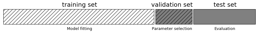
Figure 5-5. A threefold split of data into training set, validation set, and test set
After selecting the best parameters using the validation set, we can rebuild a model using the parameter settings we found, but now training on both the training data and the validation data. This way, we can use as much data as possible to build our model. This leads to the following implementation:
In[21]:
fromsklearn.svmimportSVC# split data into train+validation set and test setX_trainval,X_test,y_trainval,y_test=train_test_split(iris.data,iris.target,random_state=0)# split train+validation set into training and validation setsX_train,X_valid,y_train,y_valid=train_test_split(X_trainval,y_trainval,random_state=1)("Size of training set: {} size of validation set: {} size of test set:"" {}\n".format(X_train.shape[0],X_valid.shape[0],X_test.shape[0]))best_score=0forgammain[0.001,0.01,0.1,1,10,100]:forCin[0.001,0.01,0.1,1,10,100]:# for each combination of parameters, train an SVCsvm=SVC(gamma=gamma,C=C)svm.fit(X_train,y_train)# evaluate the SVC on the validation setscore=svm.score(X_valid,y_valid)# if we got a better score, store the score and parametersifscore>best_score:best_score=scorebest_parameters={'C':C,'gamma':gamma}# rebuild a model on the combined training and validation set,# and evaluate it on the test setsvm=SVC(**best_parameters)svm.fit(X_trainval,y_trainval)test_score=svm.score(X_test,y_test)("Best score on validation set: {:.2f}".format(best_score))("Best parameters: ",best_parameters)("Test set score with best parameters: {:.2f}".format(test_score))
Out[21]:
Size of training set: 84   size of validation set: 28   size of test set: 38

Best score on validation set: 0.96
Best parameters:  {'C': 10, 'gamma': 0.001}
Test set score with best parameters: 0.92
The best score on the validation set is 96%: slightly lower than
before, probably because we used less data to train the model (X_train
is smaller now because we split our dataset twice). However, the score
on the test set—the score that actually tells us how well we
generalize—is even lower, at 92%. So we can only claim to classify new
data 92% correctly, not 97% correctly as we thought before!
The distinction between the training set, validation set, and test set is fundamentally important to applying machine learning methods in practice. Any choices made based on the test set accuracy “leak” information from the test set into the model. Therefore, it is important to keep a separate test set, which is only used for the final evaluation. It is good practice to do all exploratory analysis and model selection using the combination of a training and a validation set, and reserve the test set for a final evaluation—this is even true for exploratory visualization. Strictly speaking, evaluating more than one model on the test set and choosing the better of the two will result in an overly optimistic estimate of how accurate the model is.
5.2.3 Grid Search with Cross-Validation
While the method of splitting the data into a training, a
validation, and a test set that we just saw is workable, and relatively commonly used, it
is quite sensitive to how exactly the data is split. From the output of
the previous code snippet we can see that grid search
selects 'C': 10, 'gamma': 0.001 as the best parameters, while the
output of the code in the previous section selects
'C': 100, 'gamma': 0.001 as the best parameters. For a better estimate
of the generalization performance, instead of using a single split into
a training and a validation set, we can use cross-validation to evaluate
the performance of each parameter combination. This method can be coded
up as follows:
In[22]:
forgammain[0.001,0.01,0.1,1,10,100]:forCin[0.001,0.01,0.1,1,10,100]:# for each combination of parameters,# train an SVCsvm=SVC(gamma=gamma,C=C)# perform cross-validationscores=cross_val_score(svm,X_trainval,y_trainval,cv=5)# compute mean cross-validation accuracyscore=np.mean(scores)# if we got a better score, store the score and parametersifscore>best_score:best_score=scorebest_parameters={'C':C,'gamma':gamma}# rebuild a model on the combined training and validation setsvm=SVC(**best_parameters)svm.fit(X_trainval,y_trainval)
To evaluate the accuracy of the SVM using a particular setting of C
and gamma using five-fold cross-validation, we need to train 36 * 5 =
180 models. As you can imagine, the main downside of the use of
cross-validation is the time it takes to train all these models.
The following visualization (Figure 5-6) illustrates how the best parameter setting is selected in the preceding code:
In[23]:
mglearn.plots.plot_cross_val_selection()
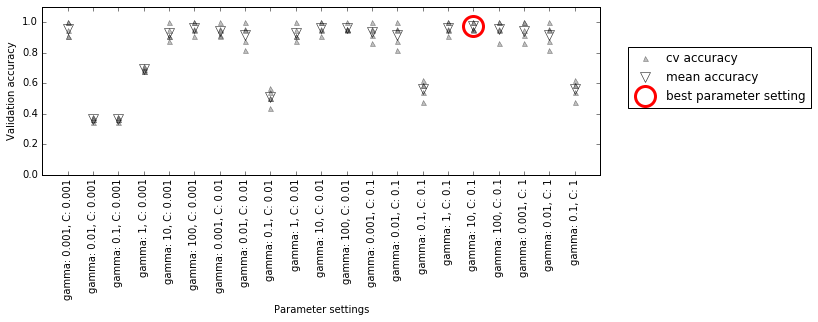
Figure 5-6. Results of grid search with cross-validation
For each parameter setting (only a subset is shown), five accuracy values are computed, one for each split in the cross-validation. Then the mean validation accuracy is computed for each parameter setting. The parameters with the highest mean validation accuracy are chosen, marked by the circle.
Warning
As we said earlier, cross-validation is a way to evaluate a given algorithm on a specific dataset. However, it is often used in conjunction with parameter search methods like grid search. For this reason, many people use the term cross-validation colloquially to refer to grid search with cross-validation.
The overall process of splitting the data, running the grid search, and evaluating the final parameters is illustrated in Figure 5-7:
In[24]:
mglearn.plots.plot_grid_search_overview()
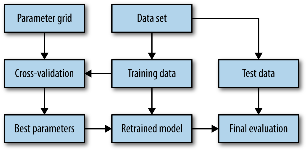
Figure 5-7. Overview of the process of parameter selection and model evaluation with GridSearchCV
Because grid search with cross-validation is such a commonly used method
to adjust parameters, scikit-learn provides the GridSearchCV class, which
implements it in the form of an estimator. To use the GridSearchCV
class, you first need to specify the parameters you want to search over
using a dictionary. GridSearchCV will then perform all the necessary
model fits. The keys of the dictionary are the names of parameters we
want to adjust (as given when constructing the model—in this case, C
and gamma), and the values are the parameter settings we want to try
out. Trying the values 0.001, 0.01, 0.1, 1, 10, and 100 for C and
gamma translates to the following dictionary:
In[25]:
param_grid={'C':[0.001,0.01,0.1,1,10,100],'gamma':[0.001,0.01,0.1,1,10,100]}("Parameter grid:\n{}".format(param_grid))
Out[25]:
Parameter grid:
{'C': [0.001, 0.01, 0.1, 1, 10, 100], 'gamma': [0.001, 0.01, 0.1, 1, 10, 100]}
We can now instantiate the GridSearchCV class with the model (SVC),
the parameter grid to search (param_grid), and the cross-validation
strategy we want to use (say, five-fold stratified cross-validation):
In[26]:
fromsklearn.model_selectionimportGridSearchCVfromsklearn.svmimportSVCgrid_search=GridSearchCV(SVC(),param_grid,cv=5,return_train_score=True)
GridSearchCV will use cross-validation in place of the split into a
training and validation set that we used before. However, we still need
to split the data into a training and a test set, to avoid overfitting
the parameters:
In[27]:
X_train,X_test,y_train,y_test=train_test_split(iris.data,iris.target,random_state=0)
The grid_search object that we created behaves just like a classifier;
we can call the standard methods fit, predict, and score on it.1 However,
when we call fit, it will run cross-validation for each combination of
parameters we specified in param_grid:
In[28]:
grid_search.fit(X_train,y_train)
Fitting the GridSearchCV object not only searches for the best
parameters, but also automatically fits a new model on the whole training
dataset with the parameters that yielded the best cross-validation
performance. What happens in fit is therefore equivalent to the result of the In[21] code we saw at the beginning of this section. The GridSearchCV class provides a
very convenient interface to access the retrained model using the
predict and score methods. To evaluate how well the best found
parameters generalize, we can call score on the test set:
In[29]:
("Test set score: {:.2f}".format(grid_search.score(X_test,y_test)))
Out[29]:
Test set score: 0.97
Choosing the parameters using cross-validation, we actually found a
model that achieves 97% accuracy on the test set. The important thing
here is that we did not use the test set to choose the parameters. The
parameters that were found are stored in the best_params_ attribute,
and the best cross-validation accuracy (the mean accuracy over the
different splits for this parameter setting) is stored in best_score_:
In[30]:
("Best parameters: {}".format(grid_search.best_params_))("Best cross-validation score: {:.2f}".format(grid_search.best_score_))
Out[30]:
Best parameters: {'C': 100, 'gamma': 0.01}
Best cross-validation score: 0.97
Warning
Again, be careful not to confuse best_score_ with the
generalization performance of the model as computed by the score
method on the test set. Using the score method (or evaluating the
output of the predict method) employs a model trained on the whole
training set. The best_score_ attribute stores the mean cross-validation accuracy, with cross-validation performed on the
training set.
Sometimes it is helpful to have access to the actual model that was
found—for example, to look at coefficients or feature importances. You
can access the model with the best parameters trained on the whole
training set using the best_estimator_ attribute:
In[31]:
("Best estimator:\n{}".format(grid_search.best_estimator_))
Out[31]:
Best estimator:
SVC(C=100, cache_size=200, class_weight=None, coef0=0.0,
  decision_function_shape='ovr', degree=3, gamma=0.01, kernel='rbf',
  max_iter=-1, probability=False, random_state=None, shrinking=True,
  tol=0.001, verbose=False)
Because grid_search itself has predict and score methods, using
best_estimator_ is not needed to make predictions or evaluate the
model.
Analyzing the result of cross-validation
It is often helpful to visualize the results of cross-validation, to
understand how the model generalization depends on the parameters we are
searching. As grid searches are quite computationally expensive to run,
often it is a good idea to start with a relatively coarse and small
grid. We can then inspect the results of the cross-validated
grid search, and possibly expand our search. The results of a grid
search can be found in the cv_results_ attribute, which is a dictionary
storing all aspects of the search. It contains a lot of details, as you can see in the following output, and
is best looked at after converting it to a pandas DataFrame:
In[32]:
importpandasaspd# convert to DataFrameresults=pd.DataFrame(grid_search.cv_results_)# show the first 5 rowsdisplay(results.head())
Out[32]:
    param_C   param_gamma   params                        mean_test_score
0   0.001     0.001         {'C': 0.001, 'gamma': 0.001}       0.366
1   0.001      0.01         {'C': 0.001, 'gamma': 0.01}        0.366
2   0.001       0.1         {'C': 0.001, 'gamma': 0.1}         0.366
3   0.001         1         {'C': 0.001, 'gamma': 1}           0.366
4   0.001        10         {'C': 0.001, 'gamma': 10}          0.366

       rank_test_score  split0_test_score  split1_test_score  split2_test_score
0               22              0.375           0.347           0.363
1               22              0.375           0.347           0.363
2               22              0.375           0.347           0.363
3               22              0.375           0.347           0.363
4               22              0.375           0.347           0.363

       split3_test_score  split4_test_score  std_test_score
0           0.363              0.380           0.011
1           0.363              0.380           0.011
2           0.363              0.380           0.011
3           0.363              0.380           0.011
4           0.363              0.380           0.011
Each row in results corresponds to one particular parameter
setting. For each setting, the results of all cross-validation splits
are recorded, as well as the mean and standard deviation over all splits. As
we were searching a two-dimensional grid of parameters (C and
gamma), this is best visualized as a heat map (Figure 5-8). First we extract the
mean validation scores, then we reshape the scores so that the axes
correspond to C and gamma:
In[33]:
scores=np.array(results.mean_test_score).reshape(6,6)# plot the mean cross-validation scoresmglearn.tools.heatmap(scores,xlabel='gamma',xticklabels=param_grid['gamma'],ylabel='C',yticklabels=param_grid['C'],cmap="viridis")
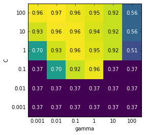
Figure 5-8. Heat map of mean cross-validation score as a function of C and gamma
Each point in the heat map corresponds to one run of cross-validation,
with a particular parameter setting. The color encodes the
cross-validation accuracy, with light colors meaning high accuracy and
dark colors meaning low accuracy. You can see that SVC is very
sensitive to the setting of the parameters. For many of the parameter
settings, the accuracy is around 40%, which is quite bad; for other
settings the accuracy is around 96%. We can take away from this plot
several things. First, the parameters we adjusted are very important
for obtaining good performance. Both parameters (C and gamma) matter a
lot, as adjusting them can change the accuracy from 40% to 96%. Additionally,
the ranges we picked for the parameters are ranges in which we see
significant changes in the outcome. It’s also important to note that the
ranges for the parameters are large enough: the optimum values for each
parameter are not on the edges of the plot.
Now let’s look at some plots (shown in Figure 5-9) where the result is less ideal, because the search ranges were not chosen properly:
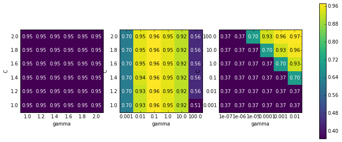
Figure 5-9. Heat map visualizations of misspecified search grids
In[34]:
fig,axes=plt.subplots(1,3,figsize=(13,5))param_grid_linear={'C':np.linspace(1,2,6),'gamma':np.linspace(1,2,6)}param_grid_one_log={'C':np.linspace(1,2,6),'gamma':np.logspace(-3,2,6)}param_grid_range={'C':np.logspace(-3,2,6),'gamma':np.logspace(-7,-2,6)}forparam_grid,axinzip([param_grid_linear,param_grid_one_log,param_grid_range],axes):grid_search=GridSearchCV(SVC(),param_grid,cv=5)grid_search.fit(X_train,y_train)scores=grid_search.cv_results_['mean_test_score'].reshape(6,6)# plot the mean cross-validation scoresscores_image=mglearn.tools.heatmap(scores,xlabel='gamma',ylabel='C',xticklabels=param_grid['gamma'],yticklabels=param_grid['C'],cmap="viridis",ax=ax)plt.colorbar(scores_image,ax=axes.tolist())
The first panel shows no changes at all, with a constant color over the
whole parameter grid. In this case, this is caused by improper scaling
and range of the parameters C and gamma. However, if no change in
accuracy is visible over the different parameter settings, it could also
be that a parameter is just not important at all. It is usually good to
try very extreme values first, to see if there are any changes in the
accuracy as a result of changing a parameter.
The second panel shows a vertical stripe pattern. This indicates that
only the setting of the gamma parameter makes any difference. This could
mean that the gamma parameter is searching over interesting values but
the C parameter is not—or it could mean the C parameter is not
important.
The third panel shows changes in both C and gamma. However, we can
see that in the entire bottom left of the plot, nothing interesting is
happening. We can probably exclude the very small values from future
grid searches. The optimum parameter setting is at the top right. As the
optimum is in the border of the plot, we can expect that there might be
even better values beyond this border, and we might want to change our
search range to include more parameters in this region.
Tuning the parameter grid based on the cross-validation scores is perfectly fine, and a good way to explore the importance of different parameters. However, you should not test different parameter ranges on the final test set—as we discussed earlier, evaluation of the test set should happen only once we know exactly what model we want to use.
Search over spaces that are not grids
In some cases, trying all possible combinations of all parameters
as GridSearchCV usually does, is not a good idea. For example, SVC
has a kernel parameter, and depending on which kernel is chosen, other parameters will be relevant. If kernel='linear', the model
is linear, and only the C parameter is used. If kernel='rbf', both
the C and gamma parameters are used (but not other parameters like
degree). In this case, searching over all possible combinations of
C, gamma, and kernel wouldn’t make sense: if kernel='linear',
gamma is not used, and trying different values for gamma would be a
waste of time. To deal with these kinds of “conditional” parameters,
GridSearchCV allows the param_grid to be a list of dictionaries.
Each dictionary in the list is expanded into an independent grid. A
possible grid search involving kernel and parameters could look like
this:
In[35]:
param_grid=[{'kernel':['rbf'],'C':[0.001,0.01,0.1,1,10,100],'gamma':[0.001,0.01,0.1,1,10,100]},{'kernel':['linear'],'C':[0.001,0.01,0.1,1,10,100]}]("List of grids:\n{}".format(param_grid))
Out[35]:
List of grids:
[{'kernel': ['rbf'], 'C': [0.001, 0.01, 0.1, 1, 10, 100],
  'gamma': [0.001, 0.01, 0.1, 1, 10, 100]},
 {'kernel': ['linear'], 'C': [0.001, 0.01, 0.1, 1, 10, 100]}]
In the first grid, the kernel parameter is always set to 'rbf' (note
that the entry for kernel is a list of length one), and both the C
and gamma parameters are varied. In the second grid, the kernel
parameter is always set to linear, and only C is varied. Now let’s
apply this more complex parameter search:
In[36]:
grid_search=GridSearchCV(SVC(),param_grid,cv=5,return_train_score=True)grid_search.fit(X_train,y_train)("Best parameters: {}".format(grid_search.best_params_))("Best cross-validation score: {:.2f}".format(grid_search.best_score_))
Out[36]:
Best parameters: {'C': 100, 'gamma': 0.01, 'kernel': 'rbf'}
Best cross-validation score: 0.97
Let’s look at the cv_results_ again. As expected, if kernel is
'linear', then only C is varied:
In[37]:
results=pd.DataFrame(grid_search.cv_results_)# we display the transposed table so that it better fits on the page:display(results.T)
Out[37]:
| 0 | 1 | 2 | 3 | … | 38 | 39 | 40 | 41 | |
|---|---|---|---|---|---|---|---|---|---|
param_C |
0.001 |
0.001 |
0.001 |
0.001 |
… |
0.1 |
1 |
10 |
100 |
param_gamma |
0.001 |
0.01 |
0.1 |
1 |
… |
NaN |
NaN |
NaN |
NaN |
param_kernel |
rbf |
rbf |
rbf |
rbf |
… |
linear |
linear |
linear |
linear |
params |
{C: 0.001, kernel: rbf, gamma: 0.001} |
{C: 0.001, kernel: rbf, gamma: 0.01} |
{C: 0.001, kernel: rbf, gamma: 0.1} |
{C: 0.001, kernel: rbf, gamma: 1} |
… |
{C: 0.1, kernel: linear} |
{C: 1, kernel: linear} |
{C: 10, kernel: linear} |
{C: 100, kernel: linear} |
mean_test_score |
0.37 |
0.37 |
0.37 |
0.37 |
… |
0.95 |
0.97 |
0.96 |
0.96 |
rank_test_score |
27 |
27 |
27 |
27 |
… |
11 |
1 |
3 |
3 |
split0_test_score |
0.38 |
0.38 |
0.38 |
0.38 |
… |
0.96 |
1 |
0.96 |
0.96 |
split1_test_score |
0.35 |
0.35 |
0.35 |
0.35 |
… |
0.91 |
0.96 |
1 |
1 |
split2_test_score |
0.36 |
0.36 |
0.36 |
0.36 |
… |
1 |
1 |
1 |
1 |
split3_test_score |
0.36 |
0.36 |
0.36 |
0.36 |
… |
0.91 |
0.95 |
0.91 |
0.91 |
split4_test_score |
0.38 |
0.38 |
0.38 |
0.38 |
… |
0.95 |
0.95 |
0.95 |
0.95 |
std_test_score |
0.011 |
0.011 |
0.011 |
0.011 |
… |
0.033 |
0.022 |
0.034 |
0.034 |
12 rows × 42 columns
Using different cross-validation strategies with grid search
Similarly to cross_val_score, GridSearchCV uses stratified k-fold
cross-validation by default for classification, and k-fold
cross-validation for regression. However, you can also pass any
cross-validation splitter, as described in “More control over cross-validation”, as the cv
parameter in GridSearchCV. In particular, to get only a single split
into a training and a validation set, you can use ShuffleSplit or
StratifiedShuffleSplit with n_splits=1. This might be helpful for very
large datasets, or very slow models.
Nested cross-validation
In the preceding examples, we went from using a single split of the data into
training, validation, and test sets to splitting the data into training
and test sets and then performing cross-validation on the training set.
But when using GridSearchCV as described earlier, we still have a single split of the
data into training and test sets, which might make our
results unstable and make us depend too much on this single split
of the data. We can go a step further, and instead of splitting the
original data into training and test sets once, use multiple
splits of cross-validation. This will result in what is called nested
cross-validation. In nested cross-validation, there is an outer loop
over splits of the data into training and test sets. For each of them, a
grid search is run (which might result in different best parameters for
each split in the outer loop). Then, for each outer split, the test set
score using the best settings is reported.
The result of this procedure is a list of scores—not a model, and not a parameter setting. The scores tell us how well a model generalizes, given the best parameters found by grid search. As it doesn’t provide a model that can be used on new data, nested cross-validation is rarely used when looking for a predictive model to apply to future data. However, it can be useful for evaluating how well a given model works on a particular dataset.
Implementing nested cross-validation in scikit-learn is straightforward.
We call cross_val_score with an instance of GridSearchCV as the
model:
In[38]:
param_grid={'C':[0.001,0.01,0.1,1,10,100],'gamma':[0.001,0.01,0.1,1,10,100]}scores=cross_val_score(GridSearchCV(SVC(),param_grid,cv=5),iris.data,iris.target,cv=5)("Cross-validation scores: ",scores)("Mean cross-validation score: ",scores.mean())
Out[38]:
Cross-validation scores:  [0.967 1.    0.967 0.967 1.   ]
Mean cross-validation score:  0.98
The result of our nested cross-validation can be summarized as “SVC can
achieve 98% mean cross-validation accuracy on the iris dataset”—nothing more and nothing less.
Here, we used stratified five-fold cross-validation in both the inner
and the outer loop. As our param_grid contains 36 combinations of
parameters, this results in a whopping 36 * 5 * 5 = 900 models being
built, making nested cross-validation a very expensive procedure. Here,
we used the same cross-validation splitter in the inner and the outer loop;
however, this is not necessary and you can use any combination of
cross-validation strategies in the inner and outer loops. It can be a bit
tricky to understand what is happening in the single line given above,
and it can be helpful to visualize it as for loops, as done in the
following simplified implementation:
In[39]:
defnested_cv(X,y,inner_cv,outer_cv,Classifier,parameter_grid):outer_scores=[]# for each split of the data in the outer cross-validation# (split method returns indices of training and test parts)fortraining_samples,test_samplesinouter_cv.split(X,y):# find best parameter using inner cross-validationbest_parms={}best_score=-np.inf# iterate over parametersforparametersinparameter_grid:# accumulate score over inner splitscv_scores=[]# iterate over inner cross-validationforinner_train,inner_testininner_cv.split(X[training_samples],y[training_samples]):# build classifier given parameters and training dataclf=Classifier(**parameters)clf.fit(X[inner_train],y[inner_train])# evaluate on inner test setscore=clf.score(X[inner_test],y[inner_test])cv_scores.append(score)# compute mean score over inner foldsmean_score=np.mean(cv_scores)ifmean_score>best_score:# if better than so far, remember parametersbest_score=mean_scorebest_params=parameters# build classifier on best parameters using outer training setclf=Classifier(**best_params)clf.fit(X[training_samples],y[training_samples])# evaluateouter_scores.append(clf.score(X[test_samples],y[test_samples]))returnnp.array(outer_scores)
Now, let’s run this function on the iris dataset:
In[40]:
fromsklearn.model_selectionimportParameterGrid,StratifiedKFoldscores=nested_cv(iris.data,iris.target,StratifiedKFold(5),StratifiedKFold(5),SVC,ParameterGrid(param_grid))("Cross-validation scores: {}".format(scores))
Out[40]:
Cross-validation scores: [0.967 1. 0.967 0.967 1. ]
Parallelizing cross-validation and grid search
While running a grid search over many parameters and on large datasets
can be computationally challenging, it is also embarrassingly
parallel. This means that building a model using a particular parameter
setting on a particular cross-validation split can be done completely
independently from the other parameter settings and models. This makes
grid search and cross-validation ideal candidates for parallelization
over multiple CPU cores or over a cluster. You can make use of multiple
cores in GridSearchCV and cross_val_score by setting the n_jobs
parameter to the number of CPU cores you want to use. You can set
n_jobs=-1 to use all available cores.
Setting n_jobs in both the model and GridSearchCV is supported since
scikit-learn 0.20.0, but is not well tested yet. If your dataset and
model are very large, it might be that using many cores uses up too much
memory, and you should monitor your memory usage when building large
models in parallel.
It is also possible to parallelize grid search and cross-validation over
multiple machines in a cluster by using the distributed computing
package dask. See http://distributed.dask.org/en/latest/joblib.html
for more details.
5.3 Evaluation Metrics and Scoring
So far, we have evaluated classification performance using accuracy (the fraction of correctly classified samples) and regression performance using R2. However, these are only two of the many possible ways to summarize how well a supervised model performs on a given dataset. In practice, these evaluation metrics might not be appropriate for your application, and it is important to choose the right metric when selecting between models and adjusting parameters.
5.3.1 Keep the End Goal in Mind
When selecting a metric, you should always have the end goal of the machine learning application in mind. In practice, we are usually interested not just in making accurate predictions, but in using these predictions as part of a larger decision-making process. Before picking a machine learning metric, you should think about the high-level goal of the application, often called the business metric. The consequences of choosing a particular algorithm for a machine learning application are called the business impact.2 Maybe the high-level goal is avoiding traffic accidents, or decreasing the number of hospital admissions. It could also be getting more users for your website, or having users spend more money in your shop. When choosing a model or adjusting parameters, you should pick the model or parameter values that have the most positive influence on the business metric. Often this is hard, as assessing the business impact of a particular model might require putting it in production in a real-life system.
In the early stages of development, and for adjusting parameters, it is often infeasible to put models into production just for testing purposes, because of the high business or personal risks that can be involved. Imagine evaluating the pedestrian avoidance capabilities of a self-driving car by just letting it drive around, without verifying it first; if your model is bad, pedestrians will be in trouble! Therefore we often need to find some surrogate evaluation procedure, using an evaluation metric that is easier to compute. For example, we could test classifying images of pedestrians against non-pedestrians and measure accuracy. Keep in mind that this is only a surrogate, and it pays off to find the closest metric to the original business goal that is feasible to evaluate. This closest metric should be used whenever possible for model evaluation and selection. The result of this evaluation might not be a single number—the consequence of your algorithm could be that you have 10% more customers, but each customer will spend 15% less—but it should capture the expected business impact of choosing one model over another.
In this section, we will first discuss metrics for the important special case of binary classification, then turn to multiclass classification and finally regression.
5.3.2 Metrics for Binary Classification
Binary classification is arguably the most common and conceptually simple application of machine learning in practice. However, there are still a number of caveats in evaluating even this simple task. Before we dive into alternative metrics, let’s have a look at the ways in which measuring accuracy might be misleading. Remember that for binary classification, we often speak of a positive class and a negative class, with the understanding that the positive class is the one we are looking for.
Kinds of errors
Often, accuracy is not a good measure of predictive performance, as the number of mistakes we make does not contain all the information we are interested in. Imagine an application to screen for the early detection of cancer using an automated test. If the test is negative, the patient will be assumed healthy, while if the test is positive, the patient will undergo additional screening. Here, we would call a positive test (an indication of cancer) the positive class, and a negative test the negative class. We can’t assume that our model will always work perfectly, and it will make mistakes. For any application, we need to ask ourselves what the consequences of these mistakes might be in the real world.
One possible mistake is that a healthy patient will be classified as positive, leading to additional testing. This leads to some costs and an inconvenience for the patient (and possibly some mental distress). An incorrect positive prediction is called a false positive. The other possible mistake is that a sick patient will be classified as negative, and will not receive further tests and treatment. The undiagnosed cancer might lead to serious health issues, and could even be fatal. A mistake of this kind—an incorrect negative prediction—is called a false negative. In statistics, a false positive is also known as type I error, and a false negative as type II error. We will stick to “false negative” and “false positive,” as they are more explicit and easier to remember. In the cancer diagnosis example, it is clear that we want to avoid false negatives as much as possible, while false positives can be viewed as more of a minor nuisance.
While this is a particularly drastic example, the consequence of false positives and false negatives are rarely the same. In commercial applications, it might be possible to assign dollar values to both kinds of mistakes, which would allow measuring the error of a particular prediction in dollars, instead of accuracy. This might be much more meaningful for making business decisions on which model to use.
Imbalanced datasets
Types of errors play an important role when one of two classes is much more frequent than the other one. This is very common in practice; a good example is click-through prediction, where each data point represents an “impression,” an item that was shown to a user. This item might be an ad, or a related story, or a related person to follow on a social media site. The goal is to predict whether, if shown a particular item, a user will click on it (indicating they are interested). Most things users are shown on the Internet (in particular, ads) will not result in a click. You might need to show a user 100 ads or articles before they find something interesting enough to click on. This results in a dataset where for each 99 “no click” data points, there is 1 “clicked” data point; in other words, 99% of the samples belong to the “no click” class. Datasets in which one class is much more frequent than the other are often called imbalanced datasets, or datasets with imbalanced classes. In reality, imbalanced data is the norm, and it is rare that the events of interest have equal or even similar frequency in the data.
Now let’s say you build a classifier that is 99% accurate on the click prediction task. What does that tell you? 99% accuracy sounds impressive, but this doesn’t take the class imbalance into account. You can achieve 99% accuracy without building a machine learning model, by always predicting “no click.” On the other hand, even with imbalanced data, a 99% accurate model could in fact be quite good. However, accuracy doesn’t allow us to distinguish the constant “no click” model from a potentially good model.
To illustrate, we’ll create a 9:1 imbalanced dataset from the digits
dataset, by classifying the digit 9 against the nine other classes:
In[41]:
fromsklearn.datasetsimportload_digitsdigits=load_digits()y=digits.target==9X_train,X_test,y_train,y_test=train_test_split(digits.data,y,random_state=0)
We can use the DummyClassifier to always predict the majority class
(here “not nine”) to see how uninformative accuracy can be:
In[42]:
fromsklearn.dummyimportDummyClassifierdummy_majority=DummyClassifier(strategy='most_frequent').fit(X_train,y_train)pred_most_frequent=dummy_majority.predict(X_test)("Unique predicted labels: {}".format(np.unique(pred_most_frequent)))("Test score: {:.2f}".format(dummy_majority.score(X_test,y_test)))
Out[42]:
Unique predicted labels: [False]
Test score: 0.90
We obtained close to 90% accuracy without learning anything. This might seem striking, but think about it for a minute. Imagine someone telling you their model is 90% accurate. You might think they did a very good job. But depending on the problem, that might be possible by just predicting one class! Let’s compare this against using an actual classifier:
In[43]:
fromsklearn.treeimportDecisionTreeClassifiertree=DecisionTreeClassifier(max_depth=2).fit(X_train,y_train)pred_tree=tree.predict(X_test)("Test score: {:.2f}".format(tree.score(X_test,y_test)))
Out[43]:
Test score: 0.92
According to accuracy, the DecisionTreeClassifier is only slightly
better than the constant predictor. This could indicate either that
something is wrong with how we used DecisionTreeClassifier, or that
accuracy is in fact not a good measure here.
For comparison purposes, let’s evaluate two more classifiers,
LogisticRegression and the default DummyClassifier, which makes
random predictions but produces classes with the same proportions as in
the training set:
In[44]:
fromsklearn.linear_modelimportLogisticRegressiondummy=DummyClassifier().fit(X_train,y_train)pred_dummy=dummy.predict(X_test)("dummy score: {:.2f}".format(dummy.score(X_test,y_test)))logreg=LogisticRegression(C=0.1).fit(X_train,y_train)pred_logreg=logreg.predict(X_test)("logreg score: {:.2f}".format(logreg.score(X_test,y_test)))
Out[44]:
dummy score: 0.80
logreg score: 0.98
The dummy classifier that produces random output is clearly the worst of
the lot (according to accuracy), while LogisticRegression produces
very good results. However, even the random classifier yields over 80%
accuracy. This makes it very hard to judge which of these results is
actually helpful. The problem here is that accuracy is an inadequate
measure for quantifying predictive performance in this imbalanced
setting. For the rest of this chapter, we will explore alternative
metrics that provide better guidance in selecting models. In particular,
we would like to have metrics that tell us how much better a model is
than making “most frequent” predictions or random predictions, as they
are computed in pred_most_frequent and pred_dummy. If we use a
metric to assess our models, it should definitely be able to weed out
these nonsense predictions.
Confusion matrices
One of the most comprehensive ways to represent the result of evaluating
binary classification is using confusion matrices.
Let’s inspect the
predictions of LogisticRegression from the previous section using the confusion_matrix
function. We already stored the predictions on the test set in
pred_logreg:
In[45]:
fromsklearn.metricsimportconfusion_matrixconfusion=confusion_matrix(y_test,pred_logreg)("Confusion matrix:\n{}".format(confusion))
Out[45]:
Confusion matrix:
[[401   2]
 [  8  39]]
The output of confusion_matrix is a two-by-two array, where the rows
correspond to the true classes and the columns correspond to the
predicted classes. Each entry counts how often a sample that belongs to
the class corresponding to the row (here, “not nine” and “nine”) was classified
as the class corresponding to the column. The following plot (Figure 5-10)
illustrates this meaning:
In[46]:
mglearn.plots.plot_confusion_matrix_illustration()
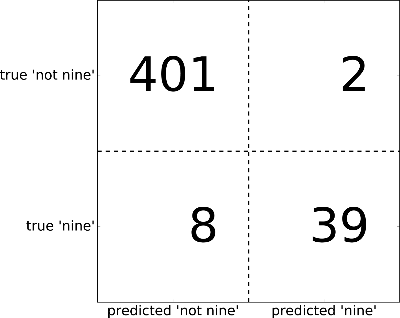
Figure 5-10. Confusion matrix of the “nine vs. rest” classification task
Entries on the main diagonal3 of the confusion matrix correspond to correct classifications, while other entries tell us how many samples of one class got mistakenly classified as another class.
If we declare “a nine” the positive class, we can relate the entries of the confusion matrix with the terms false positive and false negative that we introduced earlier. To complete the picture, we call correctly classified samples belonging to the positive class true positives and correctly classified samples belonging to the negative class true negatives. These terms are usually abbreviated FP, FN, TP, and TN and lead to the following interpretation for the confusion matrix (Figure 5-11):
In[47]:
mglearn.plots.plot_binary_confusion_matrix()
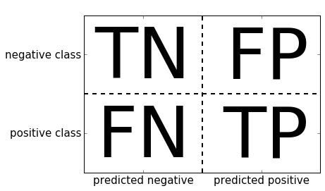
Figure 5-11. Confusion matrix for binary classification
Now let’s use the confusion matrix to compare the models we fitted earlier (the two dummy models, the decision tree, and the logistic regression):
In[48]:
("Most frequent class:")(confusion_matrix(y_test,pred_most_frequent))("\nDummy model:")(confusion_matrix(y_test,pred_dummy))("\nDecision tree:")(confusion_matrix(y_test,pred_tree))("\nLogistic Regression")(confusion_matrix(y_test,pred_logreg))
Out[48]:
Most frequent class:
[[403   0]
 [ 47   0]]

Dummy model:
[[361  42]
 [ 43   4]]

Decision tree:
[[390  13]
 [ 24  23]]

Logistic Regression
[[401   2]
 [  8  39]]
Looking at the confusion matrix, it is quite clear that something is
wrong with pred_most_frequent, because it always predicts the same
class. pred_dummy, on the other hand, has a very small number of true
positives (4), particularly compared to the number of false negatives
and false positives—there are many more false positives than true
positives! The predictions made by the decision tree make much more sense than
the dummy predictions, even though the accuracy was nearly the same.
Finally, we can see that logistic regression does better than pred_tree in
all aspects: it has more true positives and true negatives while having
fewer false positives and false negatives. From this comparison, it is
clear that only the decision tree and the logistic regression give reasonable
results, and that the logistic regression works better than the tree on
all accounts. However, inspecting the full confusion matrix is a bit
cumbersome, and while we gained a lot of insight from looking at all
aspects of the matrix, the process was very manual and qualitative.
There are several ways to summarize the information in the confusion
matrix, which we will discuss next.
Relation to accuracy
We already saw one way to summarize the result in the confusion matrix—by computing accuracy, which can be expressed as:

In other words, accuracy is the number of correct predictions (TP and TN) divided by the number of all samples (all entries of the confusion matrix summed up).
Precision, recall, and f-score
There are several other ways to summarize the confusion matrix, with the most common ones being precision and recall. Precision measures how many of the samples predicted as positive are actually positive:
Precision is used as a performance metric when the goal is to limit the number of false positives. As an example, imagine a model for predicting whether a new drug will be effective in treating a disease in clinical trials. Clinical trials are notoriously expensive, and a pharmaceutical company will only want to run an experiment if it is very sure that the drug will actually work. Therefore, it is important that the model does not produce many false positives—in other words, that it has a high precision. Precision is also known as positive predictive value (PPV).
Recall, on the other hand, measures how many of the positive samples are captured by the positive predictions:
Recall is used as performance metric when we need to identify all positive samples; that is, when it is important to avoid false negatives. The cancer diagnosis example from earlier in this chapter is a good example for this: it is important to find all people that are sick, possibly including healthy patients in the prediction. Other names for recall are sensitivity, hit rate, or true positive rate (TPR).
There is a trade-off between optimizing recall and optimizing precision. You can trivially obtain a perfect recall if you predict all samples to belong to the positive class—there will be no false negatives, and no true negatives either. However, predicting all samples as positive will result in many false positives, and therefore the precision will be very low. On the other hand, if you find a model that predicts only the single data point it is most sure about as positive and the rest as negative, then precision will be perfect (assuming this data point is in fact positive), but recall will be very bad.
Tip
Precision and recall are only two of many classification measures derived from TP, FP, TN, and FN. You can find a great summary of all the measures on Wikipedia. In the machine learning community, precision and recall are arguably the most commonly used measures for binary classification, but other communities might use other related metrics.
So, while precision and recall are very important measures, looking at only one of them will not provide you with the full picture. One way to summarize them is the f-score or f-measure, which is with the harmonic mean of precision and recall:
This particular variant is also known as the f1-score. As
it takes precision and recall into account, it can be a better measure
than accuracy on imbalanced binary classification datasets. Let’s run it
on the predictions for the “nine vs. rest” dataset that we computed
earlier. Here, we will assume that the “nine” class is the positive
class (it is labeled as True while the rest is labeled as False), so
the positive class is the minority class:
In[49]:
fromsklearn.metricsimportf1_score("f1 score most frequent: {:.2f}".format(f1_score(y_test,pred_most_frequent)))("f1 score dummy: {:.2f}".format(f1_score(y_test,pred_dummy)))("f1 score tree: {:.2f}".format(f1_score(y_test,pred_tree)))("f1 score logistic regression: {:.2f}".format(f1_score(y_test,pred_logreg)))
Out[49]:
f1 score most frequent: 0.00
f1 score dummy: 0.10
f1 score tree: 0.55
f1 score logistic regression: 0.89
We can note two things here. First, we get an error message for the most_frequent
prediction, as there were no predictions of the positive class (which
makes the denominator in the f-score zero). Also, we can see a pretty
strong distinction between the dummy predictions and the tree
predictions, which wasn’t clear when looking at accuracy alone. Using
the f-score for evaluation, we summarized the predictive performance
again in one number. However, the f-score seems to capture our intuition
of what makes a good model much better than accuracy did. A disadvantage
of the f-score, however, is that it is harder to interpret and explain
than accuracy.
If we want a more comprehensive summary of precision, recall, and f1-score, we can use the classification_report convenience function to
compute all three at once, and print them in a nice format:
In[50]:
fromsklearn.metricsimportclassification_report(classification_report(y_test,pred_most_frequent,target_names=["not nine","nine"]))
Out[50]:
              precision    recall  f1-score   support

    not nine       0.90      1.00      0.94       403
        nine       0.00      0.00      0.00        47

   micro avg       0.90      0.90      0.90       450
   macro avg       0.45      0.50      0.47       450
weighted avg       0.80      0.90      0.85       450
The classification_report function produces one line per class (here,
True and False) and reports precision, recall, and f-score with this
class as the positive class. Before, we assumed the minority “nine”
class was the positive class. If we change the positive class to “not
nine,” we can see from the output of classification_report that we
obtain an f-score of 0.94 with the most_frequent model. Furthermore,
for the “not nine” class we have a recall of 1, as we classified all
samples as “not nine.” The last column next to the f-score provides the
support of each class, which simply means the number of samples in
this class according to the ground truth.
Three additional rows in the classification report show averages of the precision, recall, and f1-score. The macro average simply computes the average across the classes, while the weighted average computes a weighted average, weighted by the number of samples in the class. Because they are averages over both classes, these metrics don’t require a notion of positive class, and in contrast to just looking at precision or just looking at recall for the positive class, averaging over both classes provides a meaningful metric in a single number. Here are two more reports, one for the dummy classifier and one for the logistic regression:
In[51]:
(classification_report(y_test,pred_dummy,target_names=["not nine","nine"]))
Out[51]:
              precision    recall  f1-score   support

    not nine       0.90      0.89      0.90       403
        nine       0.17      0.19      0.18        47

   micro avg       0.82      0.82      0.82       450
   macro avg       0.54      0.54      0.54       450
weighted avg       0.83      0.82      0.82       450
In[52]:
(classification_report(y_test,pred_logreg,target_names=["not nine","nine"]))
Out[52]:
              precision    recall  f1-score   support

    not nine       0.98      1.00      0.99       403
        nine       0.95      0.83      0.89        47

   micro avg       0.98      0.98      0.98       450
   macro avg       0.97      0.91      0.94       450
weighted avg       0.98      0.98      0.98       450
As you may notice when looking at the reports, the differences between the dummy models and a very good model are not as clear any more. Picking which class is declared the positive class has a big impact on the metrics. While the f-score for the dummy classification is 0.10 (vs. 0.89 for the logistic regression) on the “nine” class, for the “not nine” class it is 0.91 vs. 0.99, which both seem like reasonable results. Looking at all the numbers together paints a pretty accurate picture, though, and we can clearly see the superiority of the logistic regression model.
Taking uncertainty into account
The confusion matrix and the classification report provide a very
detailed analysis of a particular set of predictions. However, the
predictions themselves already threw away a lot of information that is
contained in the model. As we discussed in Chapter 2, most classifiers
provide a decision_function or a predict_proba method to assess
degrees of certainty about predictions. Making predictions can be seen
as thresholding the output of decision_function or predict_proba at
a certain fixed point—in binary classification we use 0 for the
decision function and 0.5 for predict_proba.
The following is an example of an imbalanced binary classification task, with
400 points in the negative class classified against 50 points in the
positive class. The training data is shown on the left in
Figure 5-12. We train a kernel SVM model on this data, and the
plots to the right of the training data illustrate the values of the decision
function as a heat map. You can see a black circle in the plot in the
top center, which denotes the threshold of the decision_function being
exactly zero. Points inside this circle will be classified as the
positive class, and points outside as the negative class:
In[53]:
X,y=make_blobs(n_samples=(400,50),cluster_std=[7.0,2],random_state=22)X_train,X_test,y_train,y_test=train_test_split(X,y,random_state=0)svc=SVC(gamma=.05).fit(X_train,y_train)
In[54]:
mglearn.plots.plot_decision_threshold()
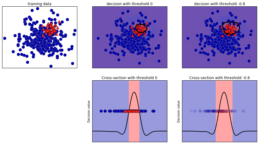
Figure 5-12. Heatmap of the decision function and the impact of changing the decision threshold
We can use the classification_report function to evaluate precision and recall
for both classes:
In[55]:
(classification_report(y_test,svc.predict(X_test)))
Out[55]:
              precision    recall  f1-score   support

           0       0.97      0.89      0.93       104
           1       0.35      0.67      0.46         9

   micro avg       0.88      0.88      0.88       113
   macro avg       0.66      0.78      0.70       113
weighted avg       0.92      0.88      0.89       113
For class 1, we get a fairly small precision, and recall is mixed. Because class 0 is so much larger, the classifier focuses on getting class 0 right, and not the smaller class 1.
Let’s assume in our application it is more important to have a high
recall for class 1, as in the cancer screening example earlier. This
means we are willing to risk more false positives (false class 1) in
exchange for more true positives (which will increase the recall). The
predictions generated by svc.predict really do not fulfill this
requirement, but we can adjust the predictions to focus on a higher
recall of class 1 by changing the decision threshold away from 0. By
default, points with a decision_function value greater than 0 will be
classified as class 1. We want more points to be classified as class
1, so we need to decrease the threshold:
In[56]:
y_pred_lower_threshold=svc.decision_function(X_test)>-.8
Let’s look at the classification report for this prediction:
In[57]:
(classification_report(y_test,y_pred_lower_threshold))
Out[57]:
              precision    recall  f1-score   support

           0       1.00      0.82      0.90       104
           1       0.32      1.00      0.49         9

   micro avg       0.83      0.83      0.83       113
   macro avg       0.66      0.91      0.69       113
weighted avg       0.95      0.83      0.87       113
As expected, the recall of class 1 went up, and the precision went down.
We are now classifying a larger region of space as class 1, as
illustrated in the top-right panel of Figure 5-12. If you value precision over recall or the other way
around, or you data is heavily imbalanced, changing the decision
threshold is the easiest way to obtain better results. As the
decision_function can have arbitrary ranges, it is hard to provide a
rule of thumb regarding how to pick a threshold. If you do set a
threshold, you need to be careful not to do so using the test set. As
with any other parameter, setting a decision threshold on the test set
is likely to yield overly optimistic results. Use a validation set or
cross-validation instead.
Warning
For simplicity, we changed the threshold value based on test set results in the code above. In practice, you need to use a hold-out validation set, not the test set. As with any other parameter, setting a decision threshold on the test set is likely to yield overly optimistic results. Use a validation set or cross-validation instead.
Picking a threshold for models that implement the predict_proba method
can be easier, as the output of predict_proba is on a fixed 0 to
1 scale, and models probabilities. By default, the threshold of 0.5
means that if the model is more than 50% “sure” that a point is of the
positive class, it will be classified as such. Increasing the threshold
means that the model needs to be more confident to make a positive
decision (and less confident to make a negative decision). While working
with probabilities may be more intuitive than working with arbitrary
thresholds, not all models provide realistic models of uncertainty (a
DecisionTree that is grown to its full depth is always 100% sure of
its decisions, even though it might often be wrong). This relates to
the concept of calibration: a calibrated model is a model that
provides an accurate measure of its uncertainty. Discussing calibration
in detail is beyond the scope of this book, but you can find
more details in the paper “Predicting Good Probabilities with Supervised
Learning” by Alexandru Niculescu-Mizil and Rich Caruana.
Precision-recall curves and ROC curves
As we just discussed, changing the threshold that is used to make a classification decision in a model is a way to adjust the trade-off of precision and recall for a given classifier. Maybe you want to miss less than 10% of positive samples, meaning a desired recall of 90%. This decision depends on the application, and it should be driven by business goals. Once a particular goal is set—say, a particular recall or precision value for a class—a threshold can be set appropriately. It is always possible to set a threshold to fulfill a particular target, like 90% recall. The hard part is to develop a model that still has reasonable precision with this threshold—if you classify everything as positive, you will have 100% recall, but your model will be useless.
Setting a requirement on a classifier like 90% recall is often called setting the operating point. Fixing an operating point is often helpful in business settings to make performance guarantees to customers or other groups inside your organization.
Often, when developing a new model, it is not entirely clear what the
operating point will be. For this reason, and to understand a modeling
problem better, it is instructive to look at all possible thresholds, or
all possible trade-offs of precision and recall at once. This is
possible using a tool called the precision-recall curve. You can find
the function to compute the precision-recall curve in the
sklearn.metrics module. It needs the ground truth labeling and
predicted uncertainties, created via either decision_function or
predict_proba:
In[58]:
fromsklearn.metricsimportprecision_recall_curveprecision,recall,thresholds=precision_recall_curve(y_test,svc.decision_function(X_test))
The precision_recall_curve function returns a list of precision and
recall values for all possible thresholds (all values that appear in the
decision function) in sorted order, so we can plot a curve, as seen in Figure 5-13:
In[59]:
# Use more data points for a smoother curveX,y=make_blobs(n_samples=(4000,500),cluster_std=[7.0,2],random_state=22)X_train,X_test,y_train,y_test=train_test_split(X,y,random_state=0)svc=SVC(gamma=.05).fit(X_train,y_train)precision,recall,thresholds=precision_recall_curve(y_test,svc.decision_function(X_test))# find threshold closest to zeroclose_zero=np.argmin(np.abs(thresholds))plt.plot(precision[close_zero],recall[close_zero],'o',markersize=10,label="threshold zero",fillstyle="none",c='k',mew=2)plt.plot(precision,recall,label="precision recall curve")plt.xlabel("Precision")plt.ylabel("Recall")plt.legend(loc="best")
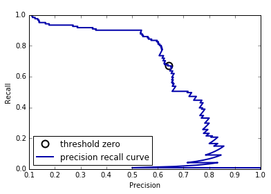
Figure 5-13. Precision recall curve for SVC(gamma=0.05)
Each point along the curve in Figure 5-13 corresponds to a
possible threshold of the decision_function. We can see, for example,
that we can achieve a recall of 0.4 at a precision of about 0.75. The
black circle marks the point that corresponds to a threshold of 0,
the default threshold for decision_function. This point is the
trade-off that is chosen when calling the predict method.
The closer a curve stays to the upper-right corner, the better the classifier. A point at the upper right means high precision and high recall for the same threshold. The curve starts at the top-left corner, corresponding to a very low threshold, classifying everything as the positive class. Raising the threshold moves the curve toward higher precision, but also lower recall. Raising the threshold more and more, we get to a situation where most of the points classified as being positive are true positives, leading to a very high precision but lower recall. The more the model keeps recall high as precision goes up, the better.
Looking at this particular curve a bit more, we can see that with this model it is possible to get a precision of up to around 0.5 with very high recall. If we want a much higher precision, we have to sacrifice a lot of recall. In other words, on the left the curve is relatively flat, meaning that recall does not go down a lot when we require increased precision. For precision greater than 0.5, each gain in precision costs us a lot of recall.
Different classifiers can work well in different parts of the curve—that is, at different operating points. Let’s compare the SVM we trained
to a random forest trained on the same dataset. The
RandomForestClassifier doesn’t have a decision_function, only
predict_proba. The precision_recall_curve function expects as its second
argument a certainty measure for the positive class (class 1), so we
pass the probability of a sample being class 1—that is,
rf.predict_proba(X_test)[:, 1]. The default threshold for
predict_proba in binary classification is 0.5, so this is the point we
marked on the curve (see Figure 5-14):
In[60]:
fromsklearn.ensembleimportRandomForestClassifierrf=RandomForestClassifier(n_estimators=100,random_state=0,max_features=2)rf.fit(X_train,y_train)# RandomForestClassifier has predict_proba, but not decision_functionprecision_rf,recall_rf,thresholds_rf=precision_recall_curve(y_test,rf.predict_proba(X_test)[:,1])plt.plot(precision,recall,label="svc")plt.plot(precision[close_zero],recall[close_zero],'o',markersize=10,label="threshold zero svc",fillstyle="none",c='k',mew=2)plt.plot(precision_rf,recall_rf,label="rf")close_default_rf=np.argmin(np.abs(thresholds_rf-0.5))plt.plot(precision_rf[close_default_rf],recall_rf[close_default_rf],'^',c='k',markersize=10,label="threshold 0.5 rf",fillstyle="none",mew=2)plt.xlabel("Precision")plt.ylabel("Recall")plt.legend(loc="best")
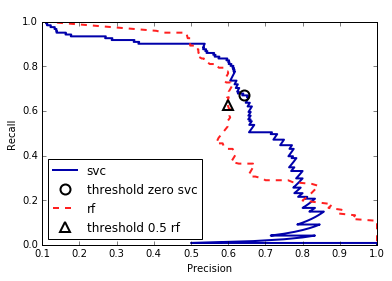
Figure 5-14. Comparing precision recall curves of SVM and random forest
From the comparison plot we can see that the random forest performs better at the extremes, for very high recall or very high precision requirements. Around the middle (approximately precision=0.7), the SVM performs better. If we only looked at the f1-score to compare overall performance, we would have missed these subtleties. The f1-score only captures one point on the precision-recall curve, the one given by the default threshold:
In[61]:
("f1_score of random forest: {:.3f}".format(f1_score(y_test,rf.predict(X_test))))("f1_score of svc: {:.3f}".format(f1_score(y_test,svc.predict(X_test))))
Out[61]:
f1_score of random forest: 0.610
f1_score of svc: 0.656
Comparing two precision-recall curves provides a lot of detailed
insight, but is a fairly manual process. For automatic model comparison,
we might want to summarize the information contained in the curve,
without limiting ourselves to a particular threshold or operating point.
One particular way to summarize the precision-recall curve is by
computing the integral or area under the curve of the precision-recall
curve, also known as the average precision.4 You can use the average_precision_score function to compute the average precision. Because we need to
compute the precision-recall curve and consider multiple thresholds, the result of decision_function or predict_proba needs to be passed to
average_precision_score, not the result of predict:
In[62]:
fromsklearn.metricsimportaverage_precision_scoreap_rf=average_precision_score(y_test,rf.predict_proba(X_test)[:,1])ap_svc=average_precision_score(y_test,svc.decision_function(X_test))("Average precision of random forest: {:.3f}".format(ap_rf))("Average precision of svc: {:.3f}".format(ap_svc))
Out[62]:
Average precision of random forest: 0.666
Average precision of svc: 0.663
When averaging over all possible thresholds, we see that the random forest
and SVC perform similarly well, with the random forest even slightly
ahead. This is quite different from the result we got from f1_score
earlier. Because average precision is the area under a curve that goes
from 0 to 1, average precision always returns a value between 0 (worst)
and 1 (best). The average precision of a classifier that assigns
decision_function at random is the fraction of positive samples in the
dataset.
Receiver operating characteristics (ROC) and AUC
There is another tool that is commonly used to analyze the behavior of classifiers at different thresholds: the receiver operating characteristics curve, or ROC curve for short. Similar to the precision-recall curve, the ROC curve considers all possible thresholds for a given classifier, but instead of reporting precision and recall, it shows the false positive rate (FPR) against the true positive rate (TPR). Recall that the true positive rate is simply another name for recall, while the false positive rate is the fraction of false positives out of all negative samples:

The ROC curve can be computed using the roc_curve function (see Figure 5-15):
In[63]:
fromsklearn.metricsimportroc_curvefpr,tpr,thresholds=roc_curve(y_test,svc.decision_function(X_test))plt.plot(fpr,tpr,label="ROC Curve")plt.xlabel("FPR")plt.ylabel("TPR (recall)")# find threshold closest to zeroclose_zero=np.argmin(np.abs(thresholds))plt.plot(fpr[close_zero],tpr[close_zero],'o',markersize=10,label="threshold zero",fillstyle="none",c='k',mew=2)plt.legend(loc=4)
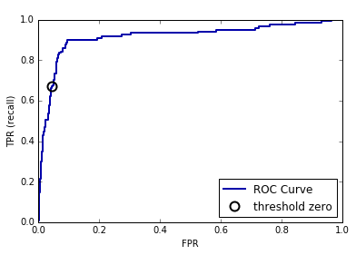
Figure 5-15. ROC curve for SVM
For the ROC curve, the ideal curve is close to the top left: you want a classifier that produces a high recall while keeping a low false positive rate. Compared to the default threshold of 0, the curve shows that we can achieve a significantly higher recall (around 0.9) while only increasing the FPR slightly. The point closest to the top left might be a better operating point than the one chosen by default. Again, be aware that choosing a threshold should not be done on the test set, but on a separate validation set.
You can find a comparison of the random forest and the SVM using ROC curves in Figure 5-16:
In[64]:
fpr_rf,tpr_rf,thresholds_rf=roc_curve(y_test,rf.predict_proba(X_test)[:,1])plt.plot(fpr,tpr,label="ROC Curve SVC")plt.plot(fpr_rf,tpr_rf,label="ROC Curve RF")plt.xlabel("FPR")plt.ylabel("TPR (recall)")plt.plot(fpr[close_zero],tpr[close_zero],'o',markersize=10,label="threshold zero SVC",fillstyle="none",c='k',mew=2)close_default_rf=np.argmin(np.abs(thresholds_rf-0.5))plt.plot(fpr_rf[close_default_rf],tpr[close_default_rf],'^',markersize=10,label="threshold 0.5 RF",fillstyle="none",c='k',mew=2)plt.legend(loc=4)
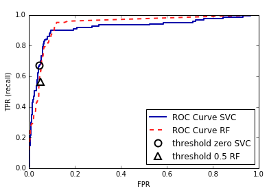
Figure 5-16. Comparing ROC curves for SVM and random forest
As for the precision-recall curve, we often want to summarize the ROC
curve using a single number, the area under the curve (this is commonly just referred to as the AUC, and it is understood that the curve in question is the ROC curve). We can
compute the area under the ROC curve using the roc_auc_score function:
In[65]:
fromsklearn.metricsimportroc_auc_scorerf_auc=roc_auc_score(y_test,rf.predict_proba(X_test)[:,1])svc_auc=roc_auc_score(y_test,svc.decision_function(X_test))("AUC for Random Forest: {:.3f}".format(rf_auc))("AUC for SVC: {:.3f}".format(svc_auc))
Out[65]:
AUC for Random Forest: 0.937
AUC for SVC: 0.916
Comparing the random forest and SVM using the AUC score, we find that the random forest performs quite a bit better than the SVM. Recall that because AUC is the area under a curve that goes from 0 to 1, AUC always returns a value between 0 (worst) and 1 (best). Predicting randomly always produces an AUC of 0.5, no matter how imbalanced the classes in a dataset are. This makes AUC a much better metric for imbalanced classification problems than accuracy. The AUC can be interpreted as evaluating the ranking of positive samples. It’s equivalent to the probability that a randomly picked point of the positive class will have a higher score according to the classifier than a randomly picked point from the negative class. So, a perfect AUC of 1 means that all positive points have a higher score than all negative points. For classification problems with imbalanced classes, using AUC for model selection is often much more meaningful than using accuracy.
Let’s go back to the problem we studied earlier of classifying all nines
in the digits dataset versus all other digits. We will classify the
dataset with an SVM with three different settings of the kernel
bandwidth, gamma (see Figure 5-17):
In[66]:
y=digits.target==9X_train,X_test,y_train,y_test=train_test_split(digits.data,y,random_state=0)plt.figure()forgammain[1,0.05,0.01]:svc=SVC(gamma=gamma).fit(X_train,y_train)accuracy=svc.score(X_test,y_test)auc=roc_auc_score(y_test,svc.decision_function(X_test))fpr,tpr,_=roc_curve(y_test,svc.decision_function(X_test))("gamma = {:.2f} accuracy = {:.2f} AUC = {:.2f}".format(gamma,accuracy,auc))plt.plot(fpr,tpr,label="gamma={:.3f}".format(gamma))plt.xlabel("FPR")plt.ylabel("TPR")plt.xlim(-0.01,1)plt.ylim(0,1.02)plt.legend(loc="best")
Out[66]:
gamma = 1.00  accuracy = 0.90  AUC = 0.50
gamma = 0.05  accuracy = 0.90  AUC = 0.90
gamma = 0.01  accuracy = 0.90  AUC = 1.00
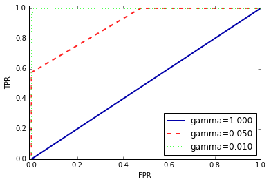
Figure 5-17. Comparing ROC curves of SVMs with different settings of gamma
The accuracy of all three settings of gamma is the same, 90%. This might be the same as chance performance, or it might not. Looking at the AUC and
the corresponding curve, however, we see a clear distinction between the
three models. With gamma=1.0, the AUC is actually at chance level,
meaning that the output of the decision_function is as good as random.
With gamma=0.05, performance drastically improves to an AUC of 0.9.
Finally, with gamma=0.01, we get a perfect AUC of 1.0. That means that
all positive points are ranked higher than all negative points according
to the decision function. In other words, with the right threshold, this
model can classify the data perfectly!5 Knowing this,
we can adjust the threshold on this model and obtain great predictions.
If we had only used accuracy, we would never have discovered this.
For this reason, we highly recommend using AUC when evaluating models on imbalanced data. Keep in mind that AUC does not make use of the default threshold, though, so adjusting the decision threshold might be necessary to obtain useful classification results from a model with a high AUC.
5.3.3 Metrics for Multiclass Classification
Now that we have discussed evaluation of binary classification tasks
in depth, let’s move on to metrics to evaluate multiclass
classification. Basically, all metrics for multiclass classification are
derived from binary classification metrics, but averaged over all
classes. Accuracy for multiclass classification is again defined as the
fraction of correctly classified examples. And again, when classes are
imbalanced, accuracy is not a great evaluation measure. Imagine a
three-class classification problem with 85% of points belonging to class
A, 10% belonging to class B, and 5% belonging to class C. What does being
85% accurate mean on this dataset? In general, multiclass
classification results are harder to understand than binary
classification results. Apart from accuracy, common tools are the
confusion matrix and the classification report we saw in the binary case in the previous section. Let’s apply these two detailed evaluation methods on the task of
classifying the 10 different handwritten digits in the digits
dataset:
In[67]:
fromsklearn.metricsimportaccuracy_scoreX_train,X_test,y_train,y_test=train_test_split(digits.data,digits.target,random_state=0)lr=LogisticRegression().fit(X_train,y_train)pred=lr.predict(X_test)("Accuracy: {:.3f}".format(accuracy_score(y_test,pred)))("Confusion matrix:\n{}".format(confusion_matrix(y_test,pred)))
Out[67]:
Accuracy: 0.953
Confusion matrix:
[[37  0  0  0  0  0  0  0  0  0]
 [ 0 39  0  0  0  0  2  0  2  0]
 [ 0  0 41  3  0  0  0  0  0  0]
 [ 0  0  1 43  0  0  0  0  0  1]
 [ 0  0  0  0 38  0  0  0  0  0]
 [ 0  1  0  0  0 47  0  0  0  0]
 [ 0  0  0  0  0  0 52  0  0  0]
 [ 0  1  0  1  1  0  0 45  0  0]
 [ 0  3  1  0  0  0  0  0 43  1]
 [ 0  0  0  1  0  1  0  0  1 44]]
The model has an accuracy of 95.3%, which already tells us that we are doing pretty well. The confusion matrix provides us with some more detail. As for the binary case, each row corresponds to a true label, and each column corresponds to a predicted label. You can find a visually more appealing plot in Figure 5-18:
In[68]:
scores_image=mglearn.tools.heatmap(confusion_matrix(y_test,pred),xlabel='Predicted label',ylabel='True label',xticklabels=digits.target_names,yticklabels=digits.target_names,cmap=plt.cm.gray_r,fmt="%d")plt.title("Confusion matrix")plt.gca().invert_yaxis()
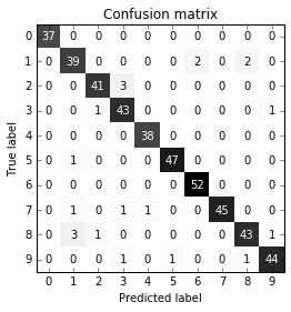
Figure 5-18. Confusion matrix for the 10-digit classification task
For the first class, the digit 0, there are 37 samples in the class, and all of these samples were classified as class 0 (there are no false negatives for class 0). We can see that because all other entries in the first row of the confusion matrix are 0. We can also see that no other digits were mistakenly classified as 0, because all other entries in the first column of the confusion matrix are 0 (there are no false positives for class 0). Some digits were confused with others, though—for example, the digit 2 (third row), three of which were classified as the digit 3 (fourth column). There was also one digit 3 that was classified as 2 (third column, fourth row) and one digit 8 that was classified as 2 (third column, ninth row).
With the classification_report function, we can compute the precision,
recall, and f-score for each class:
In[69]:
(classification_report(y_test,pred))
Out[69]:
              precision    recall  f1-score   support

           0       1.00      1.00      1.00        37
           1       0.89      0.91      0.90        43
           2       0.95      0.93      0.94        44
           3       0.90      0.96      0.92        45
           4       0.97      1.00      0.99        38
           5       0.98      0.98      0.98        48
           6       0.96      1.00      0.98        52
           7       1.00      0.94      0.97        48
           8       0.93      0.90      0.91        48
           9       0.96      0.94      0.95        47

   micro avg       0.95      0.95      0.95       450
   macro avg       0.95      0.95      0.95       450
weighted avg       0.95      0.95      0.95       450
Unsurprisingly, precision and recall are a perfect 1 for class 0, as there are no confusions with this class. For class 7, on the other hand, precision is 1 because no other class was mistakenly classified as 7, while for class 6, there are no false negatives, so the recall is 1. We can also see that the model has particular difficulties with classes 8 and 3.
The most commonly used metric for imbalanced datasets in the multiclass setting is the multiclass version of the f-score. The idea behind the multiclass f-score is to compute one binary f-score per class, with that class being the positive class and the other classes making up the negative classes. Then, these per-class f-scores are averaged using one of the following strategies:
-
"macro"averaging computes the unweighted per-class f-scores. This gives equal weight to all classes, no matter what their size is. -
"weighted"averaging computes the mean of the per-class f-scores, weighted by their support. This is what is reported in the classification report. -
"micro"averaging computes the total number of false positives, false negatives, and true positives over all classes, and then computes precision, recall, and f-score using these counts.
If you care about each sample equally much, it is recommended to use the
"micro" average f1-score; if you care about each class equally much,
it is recommended to use the "macro" average f1-score:
In[70]:
("Micro average f1 score: {:.3f}".format(f1_score(y_test,pred,average="micro")))("Macro average f1 score: {:.3f}".format(f1_score(y_test,pred,average="macro")))
Out[70]:
Micro average f1 score: 0.953
Macro average f1 score: 0.954
5.3.4 Regression Metrics
Evaluation for regression can be done in similar detail as we did for
classification—for example, by analyzing overpredicting the
target versus underpredicting the target. However, in most applications
we’ve seen, using the default R2 used in the score
method of all regressors is enough. Sometimes business decisions are
made on the basis of mean squared error or mean absolute error, which
might give incentive to tune models using these metrics. In general,
though, we have found R2 to be a more intuitive metric to
evaluate regression models.
5.3.5 Using Evaluation Metrics in Model Selection
We have discussed many evaluation methods in detail, and how to apply
them given the ground truth and a model. However, we often want to use
metrics like AUC in model selection using GridSearchCV or
cross_val_score. Luckily scikit-learn provides a very simple way to
achieve this, via the scoring argument that can be used in both
GridSearchCV and cross_val_score. You can simply provide a string
describing the evaluation metric you want to use. Say, for example, we
want to evaluate the SVM classifier on the “nine vs. rest” task on the
digits dataset, using the average precision score. Changing the score
from the default (accuracy) to average precision can be done by
providing "average_precision" as the scoring parameter:
In[71]:
# default scoring for classification is accuracy("Default scoring:",cross_val_score(SVC(),digits.data,digits.target==9,cv=5))# providing scoring="accuracy" doesn't change the resultsexplicit_accuracy=cross_val_score(SVC(),digits.data,digits.target==9,scoring="accuracy",cv=5)("Explicit accuracy:",explicit_accuracy)ap=cross_val_score(SVC(),digits.data,digits.target==9,scoring="average_precision",cv=5)("Average precision:",ap)
Out[71]:
Default scoring: [0.9 0.9 0.9 0.9 0.9]
Explicit accuracy scoring: [0.9 0.9 0.9 0.9 0.9]
AUC scoring: [0.997 0.997 0.996 0.998 0.992]
Using cross_validate, we can even compute several metrics at once:
In[72]:
res=cross_validate(SVC(),digits.data,digits.target==9,scoring=["accuracy","average_precision","recall_macro"],return_train_score=True,cv=5)display(pd.DataFrame(res))
Out[72]:
[cols=",,,,,,,,",options="header",]
|=======================================================================
| |fit_time |score_time |test_accuracy |train_accuracy
|test_average_precision |train_average_precision |test_recall_macro
|train_recall_macro
|0 |0.34 |0.20 |0.9 |1.0 |0.98 |1.0 |0.5 |1.0

|1 |0.24 |0.16 |0.9 |1.0 |1.00 |1.0 |0.5 |1.0

|2 |0.25 |0.17 |0.9 |1.0 |1.00 |1.0 |0.5 |1.0

|3 |0.23 |0.16 |0.9 |1.0 |1.00 |1.0 |0.5 |1.0

|4 |0.24 |0.15 |0.9 |1.0 |0.99 |1.0 |0.5 |1.0
|=======================================================================
Similarly, we can change the metric used to pick the best parameters in
GridSearchCV:
In[73]:
X_train,X_test,y_train,y_test=train_test_split(digits.data,digits.target==9,random_state=0)# we provide a somewhat bad grid to illustrate the point:param_grid={'gamma':[0.0001,0.01,0.1,1,10]}# using the default scoring of accuracy:grid=GridSearchCV(SVC(),param_grid=param_grid)grid.fit(X_train,y_train)("Grid-Search with accuracy")("Best parameters:",grid.best_params_)("Best cross-validation score (accuracy)): {:.3f}".format(grid.best_score_))("Test set average precision: {:.3f}".format(average_precision_score(y_test,grid.decision_function(X_test))))("Test set accuracy: {:.3f}".format(# identical to grid.score hereaccuracy_score(y_test,grid.predict(X_test))))
Out[73]:
Grid-Search with accuracy
Best parameters: {'gamma': 0.0001}
Best cross-validation score (accuracy)): 0.970
Test set average precision: 0.966
Test set accuracy: 0.973
In[74]:
# using AUC scoring instead:grid=GridSearchCV(SVC(),param_grid=param_grid,scoring="average_precision")grid.fit(X_train,y_train)("Grid-Search with average precision")("Best parameters:",grid.best_params_)("Best cross-validation score (average precision): {:.3f}".format(grid.best_score_))("Test set average precision: {:.3f}".format(# identical to grid.score hereaverage_precision_score(y_test,grid.decision_function(X_test))))("Test set accuracy: {:.3f}".format(accuracy_score(y_test,grid.predict(X_test))))
Out[74]:
Grid-Search with average precision
Best parameters: {'gamma': 0.01}
Best cross-validation score (average precision): 0.985
Test set average precision: 0.996
Test set accuracy: 0.896
When using accuracy, the parameter gamma=0.0001 is selected, while
gamma=0.01 is selected when using average precision. The
cross-validation score is consistent with the test set score in both
cases. As might be expected, the parameters found optimizing average
precision perform better on the test set in terms of average precision,
while the parameters found optimizing accuracy perform better on the
test set in terms of accuracy.
The most important values for the scoring parameter for classification
are accuracy (the default), roc_auc for the area under the ROC
curve, average_precision for the area under the precision-recall
curve, recall_macro and precision_macro for (macro) averaged
precision or recall, f1, f1_macro, and f1_weighted for the binary
f1-score and the different weighted variants. For regression, the most
commonly used values are r2 for the R2 score,
mean_squared_error for mean squared error, and mean_absolute_error
for mean absolute error. You can find a full list of supported arguments
in the documentation or by looking at the SCORER dictionary defined in
the metrics.scorer module:
In[75]:
fromsklearn.metrics.scorerimportSCORERS("Available scorers:\n{}".format(sorted(SCORERS.keys())))
Out[75]:
Available scorers:
['accuracy', 'adjusted_mutual_info_score', 'adjusted_rand_score', 'average_precision',
 'balanced_accuracy', 'brier_score_loss', 'completeness_score', 'explained_variance',
 'f1', 'f1_macro', 'f1_micro', 'f1_samples', 'f1_weighted', 'fowlkes_mallows_score',
 'homogeneity_score', 'mutual_info_score', 'neg_log_loss', 'neg_mean_absolute_error',
 'neg_mean_squared_error', 'neg_mean_squared_log_error', 'neg_median_absolute_error',
 'normalized_mutual_info_score', 'precision', 'precision_macro', 'precision_micro',
 'precision_samples', 'precision_weighted', 'r2', 'recall', 'recall_macro',
 'recall_micro', 'recall_samples', 'recall_weighted', 'roc_auc',
 'v_measure_score']
5.4 Summary and Outlook
In this chapter we discussed cross-validation, grid search, and evaluation metrics, the cornerstones of evaluating and improving machine learning algorithms. The tools described in this chapter, together with the algorithms described in Chapters 2 and 3, are the bread and butter of every machine learning practitioner.
There are two particular points that we made in this chapter that warrant repeating, because they are often overlooked by new practitioners. The first has to do with cross-validation. Cross-validation or the use of a test set allow us to evaluate a machine learning model as it will perform in the future. However, if we use the test set or cross-validation to select a model or select model parameters, we “use up” the test data, and using the same data to evaluate how well our model will do in the future will lead to overly optimistic estimates. We therefore need to resort to a split into training data for model building, validation data for model and parameter selection, and test data for model evaluation. Instead of a simple split, we can replace each of these splits with cross-validation. The most commonly used form (as described earlier) is a training/test split for evaluation, and using cross-validation on the training set for model and parameter selection.
The second point has to do with the importance of the evaluation metric or scoring function used for model selection and model evaluation. The theory of how to make business decisions from the predictions of a machine learning model is somewhat beyond the scope of this book.6 However, it is rarely the case that the end goal of a machine learning task is building a model with a high accuracy. Make sure that the metric you choose to evaluate and select a model for is a good stand-in for what the model will actually be used for. In reality, classification problems rarely have balanced classes, and often false positives and false negatives have very different consequences. Make sure you understand what these consequences are, and pick an evaluation metric accordingly.
The model evaluation and selection techniques we have described so
far are the most important tools in a data scientist’s toolbox. Grid search and cross-validation as we’ve described them in this chapter can
only be applied to a single supervised model. We have seen before,
however, that many models require preprocessing, and that in some
applications, like the face recognition example in Chapter 3, extracting
a different representation of the data can be useful. In the next
chapter, we will introduce the Pipeline class, which allows us to use
grid search and cross-validation on these complex chains of algorithms.
1 A scikit-learn estimator that is created using another estimator is called a meta-estimator. GridSearchCV is the most commonly used meta-estimator, but we will see more later.
2 We ask scientifically minded readers to excuse the commercial language in this section. Not losing track of the end goal is equally important in science, though the authors are not aware of a similar phrase to “business impact” being used in that realm.
3 The main diagonal of a two-dimensional array or matrix A is A[i, i].
4 There are some minor technical differences between the area under the precision-recall curve and average precision. However, this explanation conveys the general idea.
5 Looking at the curve for gamma=0.01 in detail, you can see a small kink close to the top left. That means that at least one point was not ranked correctly. The AUC of 1.0 is a consequence of rounding to the second decimal point.
6 We highly recommend Foster Provost and Tom Fawcett’s book Data Science for Business (O’Reilly) for more information on this topic.