Cassandra in 50 Words or Less

“Apache Cassandra is an open source, distributed, decentralized, elastically scalable, highly available, fault-tolerant, tuneably consistent, row-oriented database that bases its distribution design on Amazon’s Dynamo and its data model on Google’s Bigtable.  Created at Facebook, it is now used at some of the most popular sites on the Web.” That’s exactly 50 words.

Of course, if you were to recite that to your boss in the elevator, you’d probably get a blank look in return. So let’s break down the key points in the following sections.

Distributed and Decentralized

Cassandra is distributed, which means that it is capable of running on multiple machines while appearing to users as a unified whole.   In fact, there is little point in running a single Cassandra node. Although you can do it, and that’s acceptable for getting up to speed on how it works, you quickly realize that you’ll need multiple machines to really realize any benefit from running Cassandra. Much of its design and code base is specifically engineered toward not only making it work across many different machines, but also for optimizing performance across multiple data center racks, and even for a single Cassandra cluster running across geographically dispersed data centers. You can confidently write data to anywhere in the cluster and Cassandra will get it.

Once you start to scale many other data stores (MySQL, Bigtable), some nodes need to be set up as masters in order to organize other nodes, which are set up as slaves. Cassandra, however, is decentralized, meaning that every node is identical; no Cassandra node performs certain organizing operations distinct from any other node. Instead, Cassandra features a peer-to-peer protocol and uses gossip to maintain and keep in sync a list of nodes that are alive or dead.

The fact that Cassandra is decentralized means that there is no single point of failure. All of the nodes in a Cassandra cluster function exactly the same. This is sometimes referred to as “server symmetry.” Because they are all doing the same thing, by definition there can’t be a special host that is coordinating activities, as with the master/slave setup that you see in MySQL, Bigtable, and so many others.

In many distributed data solutions (such as RDBMS clusters), you set up multiple copies of data on different servers in a process called replication, which copies the data to multiple machines so that they can all serve simultaneous requests and improve performance. Typically this process is not decentralized, as in Cassandra, but is rather performed by defining a master/slave relationship. That is, all of the servers in this kind of cluster don’t function in the same way. You configure your cluster by designating one server as the master and others as slaves. The master acts as the authoritative source of the data, and operates in a unidirectional relationship with the slave nodes, which must synchronize their copies. If the master node fails, the whole database is in jeopardy. The decentralized design is therefore one of the keys to Cassandra’s high availability. Note that while we frequently understand master/slave replication in the RDBMS world, there are NoSQL databases such as MongoDB that follow the master/slave scheme as well.

Decentralization, therefore, has two key advantages: it’s simpler to use than master/slave, and it helps you avoid outages. It can be easier to operate and maintain a decentralized store than a master/slave store because all nodes are the same. That means that you don’t need any special knowledge to scale; setting up 50 nodes isn’t much different from setting up one. There’s next to no configuration required to support it. Moreover, in a master/slave setup, the master can become a single point of failure (SPOF). To avoid this, you often need to add some complexity to the environment in the form of multiple masters. Because all of the replicas in Cassandra are identical, failures of a node won’t disrupt service.

In short, because Cassandra is distributed and decentralized, there is no single point of failure, which supports high availability.

Elastic Scalability

Scalability is an architectural feature of a system that can continue serving a greater number of requests with little degradation in performance. Vertical scaling—simply adding more hardware capacity and memory to your existing machine—is the easiest way to achieve this. Horizontal scaling means adding more machines that have all or some of the data on them so that no one machine has to bear the entire burden of serving requests. But then the software itself must have an internal mechanism for keeping its data in sync with the other nodes in the cluster.

Elastic scalability refers to a special property of horizontal scalability. It means that your cluster can seamlessly scale up and scale back down. To do this, the cluster must be able to accept new nodes that can begin participating by getting a copy of some or all of the data and start serving new user requests without major disruption or reconfiguration of the entire cluster. You don’t have to restart your process. You don’t have to change your application queries. You don’t have to manually rebalance the data yourself. Just add another machine—Cassandra will find it and start sending it work.

Scaling down, of course, means removing some of the processing capacity from your cluster. You might do this for business reasons, such as adjusting to seasonal workloads in retail or travel applications. Or perhaps there will be technical reasons such as moving parts of your application to another platform. As much as we try to minimize these situations, they still happen. But when they do, you won’t need to upset the entire apple cart to scale back.

High Availability and Fault Tolerance

In general architecture terms, the availability of a system is measured according to its ability to fulfill requests. But computers can experience all manner of failure, from hardware component failure to network disruption to corruption. Any computer is susceptible to these kinds of failure. There are of course very sophisticated (and often prohibitively expensive) computers that can themselves mitigate many of these circumstances, as they include internal hardware redundancies and facilities to send notification of failure events and hot swap components. But anyone can accidentally break an Ethernet cable, and catastrophic events can beset a single data center. So for a system to be highly available, it must typically include multiple networked computers, and the software they’re running must then be capable of operating in a cluster and have some facility for recognizing node failures and failing over requests to another part of the system.

Cassandra is highly available. You can replace failed nodes in the cluster with no downtime, and you can replicate data to multiple data centers to offer improved local performance and prevent downtime if one data center experiences a catastrophe such as fire or flood.

Tuneable Consistency

Consistency essentially means that a read always returns the most recently written value. Consider two customers are attempting to put the same item into their shopping carts on an ecommerce site. If I place the last item in stock into my cart an instant after you do, you should get the item added to your cart, and I should be informed that the item is no longer available for purchase. This is guaranteed to happen when the state of a write is consistent among all nodes that have that data.

But as we’ll see later, scaling data stores means making certain trade-offs between data consistency, node availability, and partition tolerance. Cassandra is frequently called “eventually consistent,” which is a bit misleading. Out of the box, Cassandra trades some consistency in order to achieve total availability. But Cassandra is more accurately termed “tuneably consistent,” which means it allows you to easily decide the level of consistency you require, in balance with the level of availability.

Let’s take a moment to unpack this, as the term “eventual consistency” has caused some uproar in the industry. Some practitioners hesitate to use a system that is described as “eventually consistent.”

For detractors of eventual consistency, the broad argument goes something like this: eventual consistency is maybe OK for social web applications where data doesn’t really matter. After all, you’re just posting to Mom what little Billy ate for breakfast, and if it gets lost, it doesn’t really matter. But the data I have is actually really important, and it’s ridiculous to think that I could allow eventual consistency in my model.

Set aside the fact that all of the most popular web applications (Amazon, Facebook, Google, Twitter) are using this model, and that perhaps there’s something to it. Presumably such data is very important indeed to the companies running these applications, because that data is their primary product, and they are multibillion-dollar companies with billions of users to satisfy in a sharply competitive world. It may be possible to gain guaranteed, immediate, and perfect consistency throughout a highly trafficked system running in parallel on a variety of networks, but if you want clients to get their results sometime this year, it’s a very tricky proposition.

The detractors claim that some Big Data databases such as Cassandra have merely eventual consistency, and that all other distributed systems have strict consistency. As with so many things in the world, however, the reality is not so black and white, and the binary opposition between consistent and not-consistent is not truly reflected in practice. There are instead degrees of consistency, and in the real world they are very susceptible to external circumstance.

Eventual consistency is one of several consistency models available to architects. Let’s take a look at these models so we can understand the trade-offs:

Strict consistency

This is sometimes called sequential consistency, and is the most stringent level of consistency. It requires that any read will always return the most recently written value. That sounds perfect, and it’s exactly what I’m looking for. I’ll take it! However, upon closer examination, what do we find? What precisely is meant by “most recently written”? Most recently to whom? In one single-processor machine, this is no problem to observe, as the sequence of operations is known to the one clock. But in a system executing across a variety of geographically dispersed data centers, it becomes much more slippery. Achieving this implies some sort of global clock that is capable of timestamping all operations, regardless of the location of the data or the user requesting it or how many (possibly disparate) services are required to determine the response.

Causal consistency

This is a slightly weaker form of strict consistency. It does away with the fantasy of the single global clock that can magically synchronize all operations without creating an unbearable bottleneck. Instead of relying on timestamps, causal consistency instead takes a more semantic approach, attempting to determine the cause of events to create some consistency in their order. It means that writes that are potentially related must be read in sequence. If two different, unrelated operations suddenly write to the same field, then those writes are inferred not to be causally related. But if one write occurs after another, we might infer that they are causally related. Causal consistency dictates that causal writes must be read in sequence.

Weak (eventual) consistency

Eventual consistency means on the surface that all updates will propagate throughout all of the replicas in a distributed system, but that this may take some time. Eventually, all replicas will be consistent.

Eventual consistency becomes suddenly very attractive when you consider what is required to achieve stronger forms of consistency.

When considering consistency, availability, and partition tolerance, we can achieve only two of these goals in a given distributed system, a trade-off known as the CAP theorem (we explore this theorem in more depth in “Brewer’s CAP Theorem”). At the center of the problem is data update replication. To achieve a strict consistency, all update operations will be performed synchronously, meaning that they must block, locking all replicas until the operation is complete, and forcing competing clients to wait. A side effect of such a design is that during a failure, some of the data will be entirely unavailable. As Amazon CTO Werner Vogels puts it, “rather than dealing with the uncertainty of the correctness of an answer, the data is made unavailable until it is absolutely certain that it is correct.”¹

We could alternatively take an optimistic approach to replication, propagating updates to all replicas in the background in order to avoid blowing up on the client. The difficulty this approach presents is that now we are forced into the situation of detecting and resolving conflicts. A design approach must decide whether to resolve these conflicts at one of two possible times: during reads or during writes. That is, a distributed database designer must choose to make the system either always readable or always writable.

Dynamo and Cassandra choose to be always writable, opting to defer the complexity of reconciliation to read operations, and realize tremendous performance gains. The alternative is to reject updates amidst network and server failures.

In Cassandra, consistency is not an all-or-nothing proposition. We might more accurately term it “tuneable consistency” because the client can control the number of replicas to block on for all updates. This is done by setting the consistency level against the replication factor.

The replication factor lets you decide how much you want to pay in performance to gain more consistency. You set the replication factor to the number of nodes in the cluster you want the updates to propagate to (remember that an update means any add, update, or delete operation).

The consistency level is a setting that clients must specify on every operation and that allows you to decide how many replicas in the cluster must acknowledge a write operation or respond to a read operation in order to be considered successful. That’s the part where Cassandra has pushed the decision for determining consistency out to the client.

So if you like, you could set the consistency level to a number equal to the replication factor, and gain stronger consistency at the cost of synchronous blocking operations that wait for all nodes to be updated and declare success before returning. This is not often done in practice with Cassandra, however, for reasons that should be clear (it defeats the availability goal, would impact performance, and generally goes against the grain of why you’d want to use Cassandra in the first place). So if the client sets the consistency level to a value less than the replication factor, the update is considered successful even if some nodes are down.

Brewer’s CAP Theorem

In order to understand Cassandra’s design and its label as an “eventually consistent” database, we need to understand the CAP theorem. The CAP theorem is sometimes called Brewer’s theorem after its author, Eric Brewer.

While working at the University of California at Berkeley, Eric Brewer posited his CAP theorem in 2000 at the ACM Symposium on the Principles of Distributed Computing. The theorem states that within a large-scale distributed data system, there are three requirements that have a relationship of sliding dependency:

Consistency

All database clients will read the same value for the same query, even given concurrent updates.

Availability

All database clients will always be able to read and write data.

Partition tolerance

The database can be split into multiple machines; it can continue functioning in the face of network segmentation breaks.

Brewer’s theorem is that in any given system, you can strongly support only two of the three. This is analogous to the saying you may have heard in software development: “You can have it good, you can have it fast, you can have it cheap: pick two.”

We have to choose between them because of this sliding mutual dependency. The more consistency you demand from your system, for example, the less partition-tolerant you’re likely to be able to make it, unless you make some concessions around availability.

The CAP theorem was formally proved to be true by Seth Gilbert and Nancy Lynch of MIT in 2002. In distributed systems, however, it is very likely that you will have network partitioning, and that at some point, machines will fail and cause others to become unreachable. Networking issues such as packet loss or high latency are nearly inevitable and have the potential to cause temporary partitions. This leads us to the conclusion that a distributed system must do its best to continue operating in the face of network partitions (to be partition tolerant), leaving us with only two real options to compromise on: availability and consistency.

Figure 2-1 illustrates visually that there is no overlapping segment where all three are obtainable.

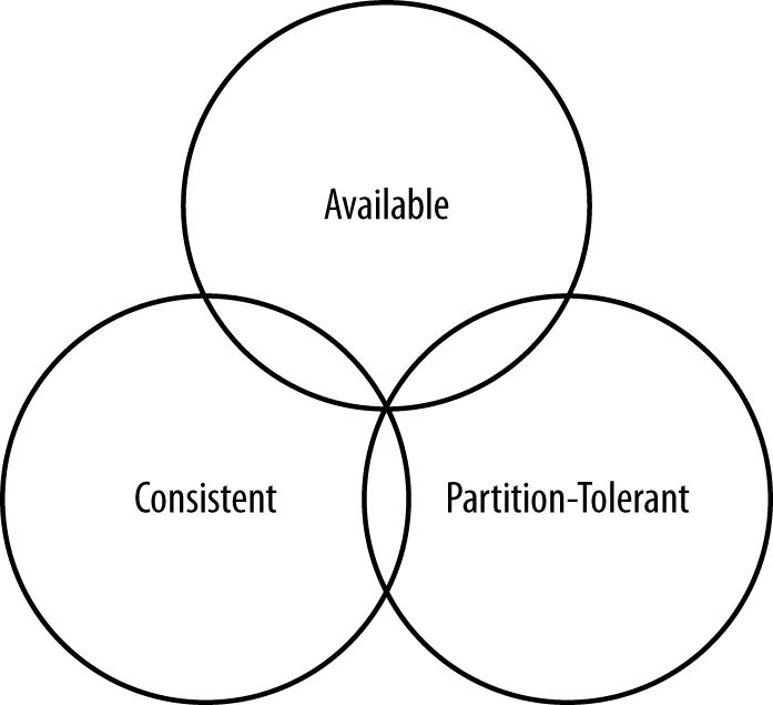
Figure 2-1. CAP theorem indicates that you can realize only two of these properties at once

It might prove useful at this point to see a graphical depiction of where each of the non-relational data stores we’ll look at falls within the CAP spectrum.  The graphic in Figure 2-2 was inspired by a slide in a 2009 talk given by Dwight Merriman, CEO and founder of MongoDB, to the MySQL User Group in New York City. However, we have modified the placement of some systems based on research.

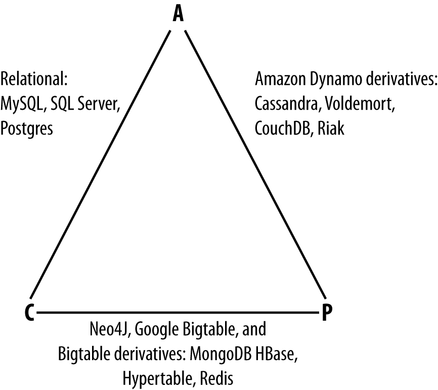
Figure 2-2. Where different databases appear on the CAP continuum

Figure 2-2 shows the general focus of some of the different databases we discuss in this chapter. Note that placement of the databases in this chart could change based on configuration. As Stu Hood points out, a distributed MySQL database can count as a consistent system only if you’re using Google’s synchronous replication patches; otherwise, it can only be available and partition tolerant (AP).

It’s interesting to note that the design of the system around CAP placement is independent of the orientation of the data storage mechanism; for example, the CP edge is populated by graph databases and document-oriented databases alike.

In this depiction, relational databases are on the line between consistency and availability, which means that they can fail in the event of a network failure (including a cable breaking). This is typically achieved by defining a single master server, which could itself go down, or an array of servers that simply don’t have sufficient mechanisms built in to continue functioning in the case of network partitions.

Graph databases such as Neo4J and the set of databases derived at least in part from the design of Google’s Bigtable database (such as MongoDB, HBase, Hypertable, and Redis) all are focused slightly less on availability and more on ensuring consistency and partition tolerance.

Finally, the databases derived from Amazon’s Dynamo design include Cassandra, Project Voldemort, CouchDB, and Riak. These are more focused on availability and partition tolerance. However, this does not mean that they dismiss consistency as unimportant, any more than Bigtable dismisses availability. According to the Bigtable paper, the average percentage of server hours that “some data” was unavailable is 0.0047% (section 4), so this is relative, as we’re talking about very robust systems already. If you think of each of these letters (C, A, P) as knobs you can tune to arrive at the system you want, Dynamo derivatives are intended for employment in the many use cases where “eventual consistency” is tolerable and where “eventual” is a matter of milliseconds, read repairs mean that reads will return consistent values, and you can achieve strong consistency if you want to.

So what does it mean in practical terms to support only two of the three facets of CAP?

CA

To primarily support consistency and availability means that you’re likely using two-phase commit for distributed transactions. It means that the system will block when a network partition occurs, so it may be that your system is limited to a single data center cluster in an attempt to mitigate this. If your application needs only this level of scale, this is easy to manage and allows you to rely on familiar, simple structures.

CP

To primarily support consistency and partition tolerance, you may try to advance your architecture by setting up data shards in order to scale. Your data will be consistent, but you still run the risk of some data becoming unavailable if nodes fail.

AP

To primarily support availability and partition tolerance, your system may return inaccurate data, but the system will always be available, even in the face of network partitioning. DNS is perhaps the most popular example of a system that is massively scalable, highly available, and partition tolerant.

Note that this depiction is intended to offer an overview that helps draw distinctions between the broader contours in these systems; it is not strictly precise. For example, it’s not entirely clear where Google’s Bigtable should be placed on such a continuum. The Google paper describes Bigtable as “highly available,” but later goes on to say that if Chubby (the Bigtable persistent lock service) “becomes unavailable for an extended period of time [caused by Chubby outages or network issues], Bigtable becomes unavailable” (section 4). On the matter of data reads, the paper says that “we do not consider the possibility of multiple copies of the same data, possibly in alternate forms due to views or indices.” Finally, the paper indicates that “centralized control and Byzantine fault tolerance are not Bigtable goals” (section 10). Given such variable information, you can see that determining where a database falls on this sliding scale is not an exact science.

Row-Oriented

Cassandra’s data model can be described as a partitioned row store, in which data is stored in sparse multidimensional hashtables. “Sparse” means that for any given row you can have one or more columns, but each row doesn’t need to have all the same columns as other rows like it (as in a relational model). “Partitioned” means that each row has a unique key which makes its data accessible, and the keys are used to distribute the rows across multiple data stores.

In the relational storage model, all of the columns for a table are defined beforehand and space is allocated for each column whether it is populated or not. In contrast, Cassandra stores data in a multidimensional, sorted hash table. As data is stored in each column, it is stored as a separate entry in the hash table. Column values are stored according to a consistent sort order, omitting columns that are not populated, which enables more efficient storage and query processing. We’ll examine Cassandra’s data model in more detail in Chapter 4.

High Performance

Cassandra was designed specifically from the ground up to take full advantage of multiprocessor/multi-core machines, and to run across many dozens of these machines housed in multiple data centers. It scales consistently and seamlessly to hundreds of terabytes. Cassandra has been shown to perform exceptionally well under heavy load. It consistently can show very fast throughput for writes per second on basic commodity computers, whether physical hardware or virtual machines. As you add more servers, you can maintain all of Cassandra’s desirable properties without sacrificing performance.

Release History

Now that we’ve learned about the people and organizations that have shaped Cassandra, let’s take a look at how Cassandra has matured through its various releases since becoming an official Apache project. If you’re new to Cassandra, don’t worry if some of these concepts and terms are new to you—we’ll dive into them in more depth in due time. You can return to this list later to get a sense of the trajectory of how Cassandra has matured over time and its future directions. If you’ve used Cassandra in the past, this summary will give you a quick primer on what’s changed.

Release 0.6

This was the first release after Cassandra graduated from the Apache Incubator to a top-level project. Releases in this series ran from 0.6.0 in April 2010 through 0.6.13 in April 2011. Features in this series included:

• Integration with Apache Hadoop, allowing easy data retrieval from Cassandra via MapReduce
• Integrated row caching, which helped eliminate the need for applications to deploy other caching technologies alongside Cassandra

Release 0.7

Releases in this series ran from 0.7.0 in January 2011 through 0.7.10 in October 2011. Key features and improvements included:

• Secondary indexes—that is, indexes on non-primary columns
• Support for large rows, containing up to two billion columns
• Online schema changes, including adding, renaming, and removing keyspaces and column families in live clusters without a restart, via the Thrift API
• Expiring columns, via specification of a time-to-live (TTL) per column
• The NetworkTopologyStrategy was introduced to support multi-data center deployments, allowing a separate replication factor per data center, per keyspace
• Configuration files were converted from XML to the more readable YAML format

Release 0.8

This release began a major shift in Cassandra APIs with the introduction of CQL. Releases in this series ran from 0.8.0 in June 2011 through 0.8.10 in February 2012. Key features and improvements included:

• Distributed counters were added as a new data type that incrementally counts up or down
• The sstableloader tool was introduced to support bulk loading of data into Cassandra clusters
• An off-heap row cache was provided to allow usage of native memory instead of the JVM heap
• Concurrent compaction allowed for multi-threaded execution and throttling control of SSTable compaction
• Improved memory configuration parameters allowed more flexible control over the size of memtables

Release 1.0

In keeping with common version numbering practice, this is officially the first production release of Cassandra, although many companies were using Cassandra in production well before this point. Releases in this series ran from 1.0.0 in October 2011 through 1.0.12 in October 2012. In keeping with the focus on production readiness, improvements focused on performance and enhancements to existing features:

• CQL 2 added several improvements, including the ability to alter tables and columns, support for counters and TTL, and the ability to retrieve the count of items matching a query
• The leveled compaction strategy was introduced as an alternative to the original size-tiered compaction strategy, allowing for faster reads at the expense of more I/O on writes
• Compression of SSTable files, configurable on a per-table level

Release 1.1

Releases in this series ran from 1.1.0 in April 2011 through 1.1.12 in May 2013. Key features and improvements included:

• CQL 3 added the timeuuid type, and the ability to create tables with compound primary keys including clustering keys. Clustering keys support “order by” semantics to allow sorting. This was a much anticipated feature that allowed the creation of “wide rows” via CQL.
• Support for importing and exporting comma-separated values (CSV) files via cqlsh
• Flexible data storage settings allow the storage of data in SSDs or magnetic storage, selectable by table
• The schema update mechanism was reimplemented to allow concurrent changes and improve reliability. Schema are now stored in tables in the system keyspace.
• Caching was updated to provide more straightforward configuration of cache sizes
• A utility to leverage the bulk loader from Hadoop, allowing efficient export of data from Hadoop to Cassandra
• Row-level isolation was added to assure that when multiple columns are updated on a write, it is not possible for a read to get a mix of new and old column values

Release 1.2

Releases in this series ran from 1.2.0 in January 2013 through 1.2.19 in September 2014. Notable features and improvements included:

• CQL 3 added collection types (sets, lists, and maps), prepared statements, and a binary protocol as a replacement for Thrift
• Virtual nodes spread data more evenly across the nodes in a cluster, improving performance, especially when adding or replacing nodes
• Atomic batches ensure that all writes in a batch succeed or fail as a unit
• The system keyspace contains the local table containing information about the local node and the peers table describing other nodes in the cluster
• Request tracing can be enabled to allow clients to see the interactions between nodes for reads and writes. Tracing provides valuable insight into what is going on behind the scenes and can help developers understand the implications of various table design options.
• Most data structures were moved off of the JVM heap to native memory
• Disk failure policies allow flexible configuration of behaviors, including removing a node from the cluster on disk failure or making a best effort to access data from memory, even if stale

Release 2.0

The 2.0 release was an especially significant milestone in the history of Cassandra, as it marked the culmination of the CQL capability, as well as a new level of production maturity. This included significant performance improvements and cleanup of the codebase to pay down 5 years of accumulated technical debt. Releases in this series ran from 2.0.0 in September 2013 through 2.0.16 in June 2015. Highlights included:

• Lightweight transactions were added using the Paxos consensus protocol
• CQL3 improvements included the addition of DROP semantics on the ALTER command, conditional schema modifications (IF EXISTS, IF NOT EXISTS), and the ability to create secondary indexes on primary key columns
• Native CQL protocol improvements began to make CQL demonstrably more performant than Thrift
• A prototype implementation of triggers was added, providing an extensible way to react to write operations. Triggers can be implemented in any JVM language.
• Java 7 was required for the first time
• Static columns were added in the 2.0.6 release

Release 2.1

Releases in this series ran from 2.1.0 in September 2014 through 2.1.8 in June 2015. Key features and improvements included:

• CQL3 added user-defined types (UDT), and the ability to create secondary indexes on collections
• Configuration options were added to move memtable data off heap to native memory
• Row caching was made more configurable to allow setting the number of cached rows per partition
• Counters were re-implemented to improve performance and reliability

Release 2.2

The original release plan outlined by the Cassandra developers did not contain a 2.2 release.  The intent was to do some major “under the covers” rework for a 3.0 release to follow the 2.1 series. However, due to the amount and complexity of the changes involved, it was decided to release some of completed features separately in order to make them available while allowing some of the more complex changes time to mature. Release 2.2.0 became available in July 2015, and support releases are scheduled through fall 2016. Notable features and improvements in this series included:

• CQL3 improvements, including support for JSON-formatted input/output and user-defined functions
• With this release, Windows became a fully supported operating system. Although Cassandra still performs best on Linux systems, improvements in file I/O and scripting have made it much easier to run Cassandra on Windows.
• The Date Tiered Compaction Strategy (DTCS) was introduced to improve performance of time series data
• Role-based access control (RBAC) was introduced to allow more flexible management of authorization

Release 3.0 (Feature release - November 2015)

• The underlying storage engine was rewritten to more closely match CQL constructs
• Support for materialized views (sometimes also called global indexes) was added
• Java 8 is now the supported version
• The Thrift-based command-line interface (CLI) was removed

Release 3.1 (Bug fix release - December 2015)

Release 3.2 (Feature release - January 2016)

• The way in which Cassandra allocates SSTable file storage across multiple disk in “just a bunch of disks” or JBOD configurations was reworked to improve reliability and performance and to enable backup and restore of individual disks
• The ability to compress and encrypt hints was added

Release 3.3 (Bug fix release - February 2016)

Release 3.4 (Feature release - March 2016)

• SSTableAttachedSecondaryIndex, or “SASI” for short, is an implementation of Cassandra’s SecondaryIndex interface that can be used as an alternative to the existing implementations.

Release 3.5 (Bug fix release - April 2016)

 

The 4.0 release series is scheduled to begin in Fall 2016.

As you will have noticed, the trends in these releases include:

• Continuous improvement in the capabilities of CQL
• A growing list of clients for popular languages built on a common set of metaphors
• Exposure of configuration options to tune performance and optimize resource usage
• Performance and reliability improvements, and reduction of technical debt

Large Deployments

You probably don’t drive a semitruck to pick up your dry cleaning; semis aren’t well suited for that sort of task. Lots of careful engineering has gone into Cassandra’s high availability, tuneable consistency, peer-to-peer protocol, and seamless scaling, which are its main selling points. None of these qualities is even meaningful in a single-node deployment, let alone allowed to realize its full potential.

There are, however, a wide variety of situations where a single-node relational database is all we may need. So do some measuring. Consider your expected traffic, throughput needs, and SLAs. There are no hard-and-fast rules here, but if you expect that you can reliably serve traffic with an acceptable level of performance with just a few relational databases, it might be a better choice to do so, simply because RDBMSs are easier to run on a single machine and are more familiar.

If you think you’ll need at least several nodes to support your efforts, however, Cassandra might be a good fit. If your application is expected to require dozens of nodes, Cassandra might be a great fit.

Lots of Writes, Statistics, and Analysis

Consider your application from the perspective of the ratio of reads to writes. Cassandra is optimized for excellent throughput on writes.

Many of the early production deployments of Cassandra involve storing user activity updates, social network usage, recommendations/reviews, and application statistics. These are strong use cases for Cassandra because they involve lots of writing with less predictable read operations, and because updates can occur unevenly with sudden spikes. In fact, the ability to handle application workloads that require high performance at significant write volumes with many concurrent client threads is one of the primary features of Cassandra.

According to the project wiki, Cassandra has been used to create a variety of applications, including a windowed time-series store, an inverted index for document searching, and a distributed job priority queue.

Geographical Distribution

Cassandra has out-of-the-box support for geographical distribution of data. You can easily configure Cassandra to replicate data across multiple data centers. If you have a globally deployed application that could see a performance benefit from putting the data near the user, Cassandra could be a great fit.

Evolving Applications

If your application is evolving rapidly and you’re in “startup mode,” Cassandra might be a good fit given its support for flexible schemas. This makes it easy to keep your database in step with application changes as you rapidly deploy.