Third Edition
A Practical Guide to the Advanced Open Source Database
Copyright © 2018 Regina Obe, Leo Hsu. All rights reserved.
Printed in the United States of America.
Published by O’Reilly Media, Inc., 1005 Gravenstein Highway North, Sebastopol, CA 95472.
O’Reilly books may be purchased for educational, business, or sales promotional use. Online editions are also available for most titles (http://oreilly.com/safari). For more information, contact our corporate/institutional sales department: 800-998-9938 or corporate@oreilly.com.
See http://oreilly.com/catalog/errata.csp?isbn=9781491963418 for release details.
The O’Reilly logo is a registered trademark of O’Reilly Media, Inc. PostgreSQL: Up and Running, the cover image, and related trade dress are trademarks of O’Reilly Media, Inc.
While the publisher and the authors have used good faith efforts to ensure that the information and instructions contained in this work are accurate, the publisher and the authors disclaim all responsibility for errors or omissions, including without limitation responsibility for damages resulting from the use of or reliance on this work. Use of the information and instructions contained in this work is at your own risk. If any code samples or other technology this work contains or describes is subject to open source licenses or the intellectual property rights of others, it is your responsibility to ensure that your use thereof complies with such licenses and/or rights.
978-1-491-96341-8
[LSI]
PostgreSQL bills itself as the world’s most advanced open source database. We couldn’t agree more.
What we hope to accomplish in this book is to give you a firm grounding in the concepts and features that make PostgreSQL so impressive. Along the way, we should convince you that PostgreSQL does indeed stand up to its claim to fame. Because the database is advanced, no book short of the 3500 pages of documentation can bring out all its glory. But then again, most users don’t need to delve into the most abstruse features that PostgreSQL has to offer. So in our shorter 300-pager, we hope to get you, as the subtitle proclaims, Up and Running.
Each topic is presented with some context so you understand when to use it and what it offers. We assume you have prior experience with some other database so that we can jump right to the key points of PostgreSQL. We generously litter the pages of this book with links to references so you can dig deeper into topics of interest. These links lead to sections in the manual, to helpful articles, to blog posts of PostgreSQL vanguards. We also link to our own site at Postgres OnLine Journal, where we have collected many pieces that we have written on PostgreSQL and its interoperability with other applications.
This book focuses on PostgreSQL versions 9.5, 9.6, and 10, but we will cover some unique and advanced features that are also present in prior versions.
For migrants from other database engines, we’ll point out parallels that PostgreSQL shares with other leading products. Perhaps more importantly, we highlight feats you can achieve with PostgreSQL that are difficult or impossible to do in other databases.
We stop short of teaching you SQL, as you’ll find many excellent sources for that. SQL is much like chess—a few hours to learn, a lifetime to master. You have wisely chosen PostgreSQL. You’ll be greatly rewarded.
If you’re currently a savvy PostgreSQL user or a weather-beaten DBA, much of the material in this book should be familiar terrain, but you’ll be sure to pick up some pointers and shortcuts introduced in newer versions of PostgreSQL. Perhaps you’ll even find the hidden gem that eluded you. If nothing else, this book is at least ten times lighter than the PostgreSQL manual.
Not using PostgreSQL yet? This book is propaganda—the good kind. Each day you continue to use a database with limited SQL capabilities, you handicap yourself. Each day that you’re wedded to a proprietary system, you’re bleeding dollars.
Finally, if your work has nothing to do with databases or IT, or if you’ve just graduated from kindergarten, the cute picture of the elephant shrew on the cover should be worthy of the price alone.
PostgreSQL has a well-maintained set of online documentation: PostgreSQL manuals. We encourage you to bookmark it. The manual is available both as HTML and as a PDF. Hardcopy collector editions are available for purchase.
Other PostgreSQL resources include:
Planet PostgreSQL is an aggregator of PostgreSQL blogs. You’ll find PostgreSQL core developers and general users showcasing new features, novel ways to use existing ones, and reporting of bugs that have yet to be patched.
PostgreSQL Wiki provides tips and tricks for managing various facets of the database and migrating from other databases.
PostgreSQL Books is a list of books about PostgreSQL.
PostGIS in Action Books is the website for the books we’ve written on PostGIS, the spatial extender for PostgreSQL, and more recently pgRouting, another PostgreSQL extension that provides network routing capabilities useful for building driving apps.
For elements in parentheses, we gravitate toward placing the open parenthesis on the same line as the preceding element and the closing parenthesis on a line by itself. This is a classic C formatting style that we like because it cuts down on the number of blank lines:
function(
	Welcome to PostgreSQL
);
We also remove gratuitous spaces in screen output, so if the formatting of your results doesn’t match ours exactly, don’t fret.
We omit the space after a serial comma for short elements. For example, ('a','b','c').
The SQL interpreter treats tabs, newlines, and carriage returns as whitespace. In our code, we generally use whitespaces for indentation, not tabs. Make sure that your editor doesn’t automatically remove tabs, newlines, and carriage returns or convert them to something other than spaces.
After copying and pasting, if you find your code not working, check the copied code to make sure it looks like what we have in the listing.
We use examples based on both Linux and Windows. Path notations
differ between the two, namely the use of solidus (/) versus
reverse solidus (\). While on Windows, use the Linux solidus,
always! /, not \. You may see a path such as
/postgresql_book/somefile.csv. These are always
relative to the root of your server. If you are on Windows, you must
include the drive letter:
C:/postgresql_book/somefile.csv.
The following typographical conventions are used in this book:
Indicates new terms, URLs, email addresses, filenames, and file extensions.
Constant widthUsed for program listings. Used within paragraphs, where needed for clarity, to refer to programming elements such as variables, functions, databases, data types, environment variables, statements, and keywords.
Constant width
        bold
Shows commands or other text that should be typed literally by the user.
Constant width italicShows text that should be replaced with user-supplied values or by values determined by context.
This icon signifies a tip, suggestion, or general note.
This icon indicates a warning or caution.
Code and data examples are available for download at http://www.postgresonline.com/downloads/postgresql_book_3e.zip.
This book is here to help you get your job done. In general, you may use the code in this book in your programs and documentation. You do not need to contact us for permission unless you’re reproducing a significant portion of the code. For example, writing a program that uses several chunks of code from this book does not require permission. Selling or distributing a CD-ROM of examples from O’Reilly books does require permission. Answering a question by citing this book and quoting example code does not require permission. Incorporating a significant amount of example code from this book into your product’s documentation does require permission.
We appreciate, but do not require, attribution. An attribution usually includes the title, author, publisher, and ISBN. For example: “PostgreSQL: Up and Running, Third Edition by Regina Obe and Leo Hsu (O’Reilly). Copyright 2018 Regina Obe and Leo Hsu, 978-1-491-96341-8.”
If you feel your use of code examples falls outside fair use or the permission given above, feel free to contact us at permissions@oreilly.com.
Safari (formerly Safari Books Online) is a membership-based training and reference platform for enterprise, government, educators, and individuals.
Members have access to thousands of books, training videos, Learning Paths, interactive tutorials, and curated playlists from over 250 publishers, including O’Reilly Media, Harvard Business Review, Prentice Hall Professional, Addison-Wesley Professional, Microsoft Press, Sams, Que, Peachpit Press, Adobe, Focal Press, Cisco Press, John Wiley & Sons, Syngress, Morgan Kaufmann, IBM Redbooks, Packt, Adobe Press, FT Press, Apress, Manning, New Riders, McGraw-Hill, Jones & Bartlett, and Course Technology, among others.
For more information, please visit http://oreilly.com/safari.
Please address comments and questions concerning this book to the publisher:
Please submit errata using the book’s errata page.
The companion site for this book is at http://bit.ly/postgresql-up-and-running-3e.
To contact the authors, send email to lr@pcorp.us.
To comment or ask technical questions to the publisher, send email to bookquestions@oreilly.com.
For more information about our books, courses, conferences, and news, see our website at http://www.oreilly.com.
Find us on Facebook: http://facebook.com/oreilly
Follow us on Twitter: http://twitter.com/oreillymedia
Watch us on YouTube: http://www.youtube.com/oreillymedia
PostgreSQL is an extremely powerful piece of software that introduces features you may not have seen before. Some of the features are also present in other well-known database engines, but under different names. This chapter lays out the main concepts you should know when starting to attack PostgreSQL documentation, and mentions some related terms in other databases.
We begin by pointing you to resources for downloading and installing PostgreSQL. Next, we provide an overview of indispensable administration tools followed by a review of PostgreSQL nomenclature. PostgreSQL 10 was recently released. We’ll highlight some of the new features therein. We close with resources to turn to when you need additional guidance and to submit bug reports.
PostgreSQL is an enterprise-class relational database management system, on par with the very best proprietary database systems: Oracle, Microsoft SQL Server, and IBM DB2, just to name a few. PostgreSQL is special because it’s not just a database: it’s also an application platform, and an impressive one at that.
PostgreSQL is fast. In benchmarks, PostgreSQL either exceeds or matches the performance of many other databases, both open source and proprietary.
PostgreSQL invites you to write stored procedures and functions in numerous programming languages. In addition to the prepackaged languages of C, SQL, and PL/pgSQL, you can easily enable support for additional languages such as PL/Perl, PL/Python, PL/V8 (aka PL/JavaScript), PL/Ruby, and PL/R. This support for a wide variety of languages allows you to choose the language with constructs that can best solve the problem at hand. For instance, use R for statistics and graphing, Python for calling web services, the Python SciPy library for scientific computing, and PL/V8 for validating data, processing strings, and wrangling with JSON data. Easier yet, find a freely available function that you need, find out the language that it’s written in, enable that specific language in PostgreSQL, and copy the code. No one will think less of you.
Most database products limit you to a predefined set of data types: integers, texts, Booleans, etc. Not only does PostgreSQL come with a larger built-in set than most, but you can define additional data types to suit your needs. Need complex numbers? Create a composite type made up of two floats. Have a triangle fetish? Create a coordinate type, then create a triangle type made up of three coordinate pairs. A dozenal activist? Create your own duodecimal type. Innovative types are useful insofar as the operators and functions that support them. So once you’ve created your special number types, don’t forget to define basic arithmetic operations for them. Yes, PostgreSQL will let you customize the meaning of the symbols (+,-,/,*). Whenever you create a type, PostgreSQL automatically creates a companion array type for you. If you created a complex number type, arrays of complex numbers are available to you without additional work.
PostgreSQL also automatically creates types from any tables you define. For instance, create a table of dogs with columns such as breed, cuteness, and barkiness. Behind the scenes, PostgreSQL maintains a dogs data type for you. This amazingly useful bridge between the relational world and the object world means that you can treat data elements in a way that’s convenient for the task at hand. You can create functions that work on one object at a time or functions that work on sets of objects at a time. Many third-party extensions for PostgreSQL leverage custom types to achieve performance gains, provide domain-specific constructs for shorter and more maintainable code, and accomplish feats you can only fantasize about with other database products.
Our principal advice is this: don’t treat databases as dumb storage. A database such as PostgreSQL can be a full-fledged application platform. With a robust database, everything else is eye candy. Once you’re versant in SQL, you’ll be able to accomplish in seconds what would take a casual programmer hours, both in coding and running time.
In recent years, we’ve witnessed an upsurge of NoSQL movements (though much of it could be hype). Although PostgreSQL is fundamentally relational, you’ll find plenty of facilities to handle nonrelational data. The ltree extension to PostgreSQL has been around since time immemorial and provides support for graphs. The hstore extensions let you store key-value pairs. JSON and JSONB types allow storage of documents similar to MongoDb. In many ways, PostgreSQL accommodated NoSQL before the term was even coined!
PostgreSQL just celebrated its 20th birthday, dating from its christening to PostgreSQL from Postgres95. The beginnings of the PostgreSQL code-base began well before that in 1986. PostgreSQL is supported on all major operating systems: Linux, Unix, Windows, and Mac. Every year brings a new major release, offering enhanced performance along with features that push the envelope of what’s possible in a database offering.
Finally, PostgreSQL is open source with a generous licensing policy. PostgreSQL is supported by a community of developers and users where profit maximization is not the ultimate pursuit. If you want features, you’re free to contribute, or at least vocalize. If you want to customize and experiment, no one is going to sue you. You, the mighty user, make PostgreSQL what it is.
In the end, you will wonder why you ever used any other database, because PostgreSQL does everything you could hope for and does it for free. No more reading the licensing cost fineprint of those other databases to figure out how many dollars you need to spend if you have eight cores on your virtualized servers with X number of concurrent connections. No more fretting about how much more the next upgrade will cost you.
Given all the proselytizing thus far, it’s only fair that we point out situations when PostgreSQL might not be suitable.
The typical installation size of PostgreSQL without any extensions is more than 100 MB. This rules out PostgreSQL for a database on a small device or as a simple cache store. Many lightweight databases abound that could better serve your needs without the larger footprint.
Given its enterprise stature, PostgreSQL doesn’t take security lightly. If you’re developing lightweight applications where you’re managing security at the application level, PostgreSQL security with its sophisticated role and permission management could be overkill. You might consider a single-user database such as SQLite or a database such as Firebird that can be run either as a client server or in single-user embedded mode.
All that said, it is a common practice to combine PostgreSQL with other database types. One common combination you will find is using Redis or Memcache to cache PostgreSQL query results. As another example, SQLite can be used to store a disconnected set of data for offline querying when PostgreSQL is the main database backend for an application.
Finally, many hosting companies don’t offer PostgreSQL on a shared hosting environment, or they offer an outdated version. Most still gravitate toward the impotent MySQL. To a web designer, for whom the database is an afterthought, MySQL might suffice. But as soon as you learn to write any SQL beyond a single-table select and simple joins, you’ll begin to sense the shortcomings of MySQL. Since the first edition of this book, virtualization has resown the landscape of commerical hosting, so having your own dedicated server is no longer a luxury, but the norm. And when you have your own server, you’re free to choose what you wish to have installed. PostgreSQL bodes well with the popularity of cloud computing such as Platform as a Service (PaaS) and Database as a Service (DbaaS). Most of the major PaaS and DbaaS providers offer PostgreSQL, notably Heroku, Engine Yard, Red Hat OpenShift, Amazon RDS for PostgreSQL, Google Cloud SQL for PostgreSQL, Amazon Aurora for PostgreSQL, and Microsoft Azure for PostgreSQL.
Years ago, if you wanted PostgreSQL, you had to compile it from source. Thankfully, those days are long gone. Granted, you can still compile from source, but using packaged installers won’t make you any less cool. A few clicks or keystrokes, and you’re on your way.
If you’re installing PostgreSQL for the first time and have no existing database to upgrade, you should install the latest stable release version for your OS. The downloads page for the PostgreSQL core distribution maintains a listing of places where you can download PostgreSQL binaries for various OSes. In Appendix A, you’ll find useful installation instructions and links to additional custom distributions.
Four tools widely used with PostgreSQL are psql, pgAdmin, phpPgAdmin, and Adminer. PostgreSQL core developers actively maintain the first three; therefore, they tend to stay in sync with PostgreSQL releases. Adminer, while not specific to PostgreSQL, is useful if you also need to manage other relational databases: SQLite, MySQL, SQL Server, or Oracle. Beyond the four that we mentioned, you can find plenty of other excellent administration tools, both open source and proprietary.
psql is a command-line interface for running queries and is included in all distributions of PostgreSQL (see “psql Interactive Commands”). psql has some unusual features, such as an import and export command for delimited files (CSV or tab), and a minimalistic report writer that can generate HTML output. psql has been around since the introduction of PostgreSQL and is the tool of choice for many expert users, for people working in consoles without a GUI, or for running common tasks in shell scripts. Newer converts favor GUI tools and wonder why the older generation still clings to the command line.
pgAdmin is a popular, free GUI tool for PostgreSQL. Download it separately from PostgreSQL if it isn’t already packaged with your installer. pgAdmin runs on all OSes supported by PostgreSQL.
Even if your database lives on a console-only Linux server, go ahead and install pgAdmin on your workstation, and you’ll find yourself armed with a fantastic GUI tool.
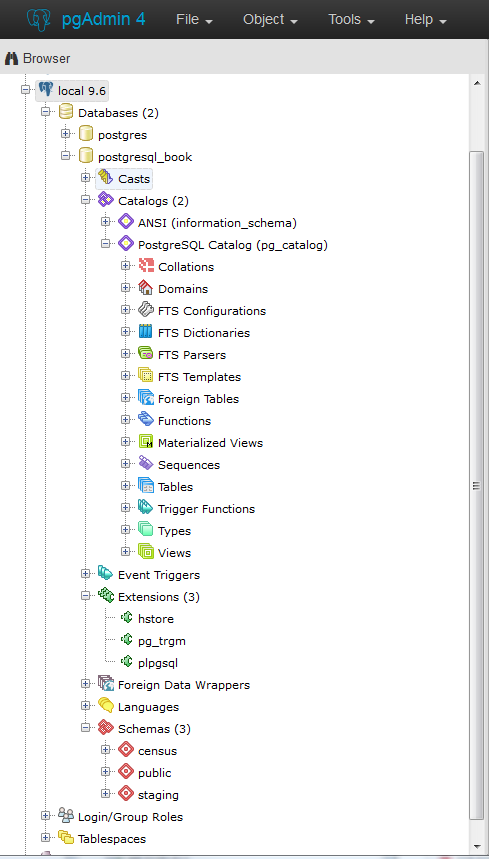
pgAdmin recently entered its fourth release, dubbed pgAdmin4. pgAdmin4 is a complete rewrite of pgAdmin3 that sports a desktop as well as a web server application version utilizing Python. pgAdmin4 is currently at version 1.5. It made its debut at the same time as PostgreSQL 9.6 and is available as part of several PostgreSQL distributions. You can run pgAdmin4 as a desktop application or via a browser interface.
An example of pgAdmin4 appears in Figure 1-1.
If you’re unfamiliar with PostgreSQL, you should definitely start with pgAdmin. You’ll get a bird’s-eye view and appreciate the richness of PostgreSQL just by exploring everything you see in the main interface. If you’re deserting Microsoft SQL Server and are accustomed to Management Studio, you’ll feel right at home.
pgAdmin4 still has a couple of pain points compared to pgAdmin3, but its feature set is ramping up quickly and in some ways already surpasses pgAdmin3. That said, if you are a long-time user of pgAdmin3, you might want to go for the pgAdmin3 Long Time support (LTS) version supported and distributed by BigSQL, and spend a little time test-driving pgAdmin4 before you fully commit to it. But keep in mind that the pgAdmin project is fully committed to pgAdmin4 and no longer will make changes to pgAdmin3.
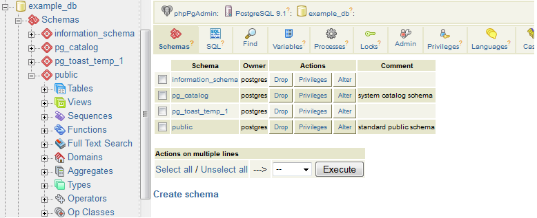
phpPgAdmin, pictured in Figure 1-2, is a free, web-based administration tool patterned after the popular phpMyAdmin. phpPgAdmin differs from phpMyAdmin by including ways to manage PostgreSQL objects such as schemas, procedural languages, casts, operators, and so on. If you’ve used phpMyAdmin, you’ll find phpPgAdmin to have the same look and feel.
If you manage other databases besides PostgreSQL and are looking for a unified tool, Adminer might fit the bill. Adminer is a lightweight, open source PHP application with options for PostgreSQL, MySQL, SQLite, SQL Server, and Oracle, all delivered through a single interface.
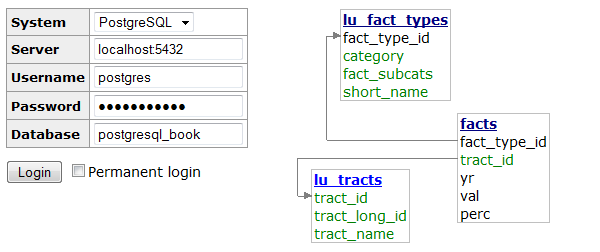
One unique feature of Adminer we’re impressed with is the relational diagrammer that can produce a schematic layout of your database schema, along with a linear representation of foreign key relationships. Another hassle-reducing feature is that you can deploy Adminer as a single PHP file.
Figure 1-3 is a screenshot of the login screen and a snippet from the diagrammer output. Many users stumble in the login screen of Adminer because it doesn’t include a separate text box for indicating the port number. If PostgreSQL is listening on the standard 5432 port, you need not worry. But if you use some other port, append the port number to the server name with a colon, as shown in Figure 1-3.
Adminer is sufficient for straightforward querying and editing, but because it’s tailored to the lowest common denominator among database products, you won’t find management applets that are specific to PostgreSQL for such tasks as creating new users, granting rights, or displaying permissions. Adminer also treats each schema as a separate database, which severely reduces the usefulness of the relational diagrammer if your relationships cross schema boundaries. If you’re a DBA, stick to pgAdmin or psql.
So you installed PostgreSQL, fired up pgAdmin, and expanded its browse tree. Before you is a bewildering display of database objects, some familiar and some completely foreign. PostgreSQL has more database objects than most other relational database products (and that’s before add-ons). You’ll probably never touch many of these objects, but if you dream up something new, more likely than not it’s already implemented using one of those esoteric objects. This book is not even going to attempt to describe all that you’ll find in a standard PostgreSQL install. With PostgreSQL churning out features at breakneck speed, we can’t imagine any book that could possibly do this. We limit our quick overview to those objects that you should be familiar with:
Schemas are part of the ANSI SQL standard. They are the immediate next level of organization within each database. If you think of the database as a country, schemas would be the individual states (or provinces, prefectures, or departments, depending on the country). Most database objects first belong to a schema, which belongs to a database. When you create a new database, PostgreSQL automatically creates a schema named public to store objects that you create. If you have few tables, using public would be fine. But if you have thousands of tables, you should organize them into different schemas.
Tables are the workhorses of any database. In PostgreSQL, tables are first citizens of their respective schemas, which in turn are citizens of the database.
PostgreSQL tables have two remarkable talents: first, they are inheritable. Table inheritance streamlines your database design and can save you endless lines of looping code when querying tables with nearly identical structures. Second, whenever you create a table, PostgreSQL automatically creates an accompanying custom data type.
Almost all relational database products offer views as a level of abstraction from tables. In a view, you can query multiple tables and present additional derived columns based on complex calculations. Views are generally read-only, but PostgreSQL allows you to update the underlying data by updating the view, provided that the view draws from a single table. To update data from views that join multiple tables, you need to create a trigger against the view. Version 9.3 introduced materialized views, which cache data to speed up commonly used queries at the sacrifice of having the most up-to-date data. See “Materialized Views”.
Extensions allow developers to package functions, data types, casts,
custom index types, tables, attribute variables, etc., for
installation or removal as a unit. Extensions are similar in concept
to Oracle packages and have been the preferred method for
distributing add-ons since PostgreSQL 9.1. You should follow the
developer’s instructions on how to install the extension files onto
your server, which usually involves copying binaries into your
PostgreSQL installation folders and then running a set of scripts.
Once done, you must enable the extension for each database
separately. You shouldn’t enable an extension in your database
unless you need it. For example, if you need advanced text search in
only one database, enable fuzzystrmatch for that one
only.
When you enable extensions, you choose the schemas where all constituent objects will reside. Accepting the default will place everything from the extension into the public schema, littering it with potentially thousands of new objects. We recommend that you create a separate schema that will house all extensions. For an extension with many objects, we suggest that you create a separate schema devoted entirely to it. Optionally, you can append the name of any schemas you add to the search_path variable of the database so you can refer to the function without having to prepend the schema name. Some extensions, especially ones that install a new procedural language (PL), will dictate the installation schema. For example, PL/V8 must be installed the pg_catalog schema.
Extensions may depend on other extensions. Prior to PostgreSQL
9.6, you had to know all dependent extensions and install them
first. With 9.6, you simply need to add the CASCADE
option and PostgreSQL will take care of the rest. For example:
CREATEEXTENSIONpostgis_tiger_geocoderCASCADE;
first installs the dependent extensions postgis and fuzzystrmatch, if not present.
You can program your own custom functions to handle data manipulation, perform complex calculations, or wrap similar functionality. Create functions using PLs. PostgreSQL comes stocked with thousands of functions, which you can view in the postgres database that is part of every install. PostgreSQL functions can return scalar values, arrays, single records, or sets of records. Other database products refer to functions that manipulate data as stored procedures. PostgreSQL does not make this distinction.
Create functions using a PL. PostgreSQL installs three by default: SQL,
PL/pgSQL, and C. You can easily install additional languages using
the extension framework or the CREATE PRODCEDURAL LANGUAGE command.
Languages currently in vogue are PL/Python, PL/V8 (JavaScript), and
PL/R. We’ll show you plenty of examples in Chapter 8.
Operators are nothing more than symbolically named aliases such as = or && for functions. In PostgreSQL, you can invent your own. This is often the case when you create custom data types. For example, if you create a custom data type of complex numbers, you’d probably want to also create addition operators (+,-,*,/) to handle arithmetic on them.
Foreign tables are virtual tables linked to data outside a PostgreSQL database. Once you’ve configured the link, you can query them like any other tables. Foreign tables can link to CSV files, a PostgreSQL table on another server, a table in a different product such as SQL Server or Oracle, a NoSQL database such as Redis, or even a web service such as Twitter or Salesforce.
Foreign data wrappers (FDWs) facilitate the magic handshake between PostgreSQL and external data sources. FDW implementations in PostgreSQL follow the SQL/Management of External Data (MED) standard.
Many charitable programmers have already developed FDWs for popular data sources. You can try your hand at creating your own FDWs as well. (Be sure to publicize your success so the community can reap the fruits of your toil.) Install FDWs using the extension framework. Once installed, pgAdmin lists them under a node called Foreign Data Wrappers.
You will find triggers in all enterprise-level databases; triggers detect data-change events. When PostgreSQL fires a trigger, you have the opportunity to execute trigger functions in response. A trigger can run in response to particular types of statements or in response to changes to particular rows, and can fire before or after a data-change event.
In pgAdmin, to see which table triggers, drill down to the table level. Pick the table of interest and look under triggers.
Create trigger functions to respond to firing of triggers. Trigger functions differ from regular functions in that they have access to special variables that store the data both before and after the triggering event. This allows you to reverse data changes made by the event during the execution of the trigger function. Because of this, trigger functions are often used to write complex validation routines that are beyond what can be implemented using check constraints.
Trigger technology is evolving rapidly in PostgreSQL. Starting in 9.0, a WITH clause lets you specify a boolean WHEN condition, which is tested to see whether the trigger should be fired. Version 9.0 also introduced the UPDATE OF clause, which allows you to specify which column(s) to monitor for changes. When data in monitored columns changes, the trigger fires. In 9.1, a data change in a view can fire a trigger. Since 9.3, data definition language (DDL) events can fire triggers. For a list of triggerable DDL events, refer to the Event Trigger Firing Matrix. pgAdmin lists DDL triggers under the Event Triggers branch. Finally, as of version 9.4, you may place triggers against foreign tables.
Catalogs are system schemas that store PostgreSQL builtin functions and metadata. Every database contains two catalogs: pg_catalog, which holds all functions, tables, system views, casts, and types packaged with PostgreSQL; and information_schema, which offers views exposing metadata in a format dictated by the ANSI SQL standard.
PostgreSQL practices what it preaches. You will find that PostgreSQL itself is built atop a self-replicating structure. All settings to finetune servers are kept in system tables that you’re free to query and modify. This gives PostgreSQL a level of extensibility (read hackability) impossible to attain by proprietary database products. Go ahead and take a close look inside the pg_catalog schema. You’ll get a sense of how PostgreSQL is put together. If you have superuser privileges, you are at liberty to make updates to the pg_catalog directly (and screw things up royally).
The information_schema catalog is one you’ll find in MySQL and SQL Server as well. The most commonly used views in the PostgreSQL information_schema are columns, which list all table columns in a database; tables, which list all tables (including views) in a database; and views, which list all views and the associated SQL to rebuild the view.
Type is short for data type. Every database product and every programming language has a set of types that it understands: integers, characters, arrays, blobs, etc. PostgreSQL has composite types, which are made up of other types. Think of complex numbers, polar coordinates, vectors, or tensors as examples.
Whenever you create a new table, PostgreSQL automatically creates a composite type based on the structure of the table. This allows you to treat table rows as objects in their own right. You’ll appreciate this automatic type creation when you write functions that loop through tables. pgAdmin doesn’t make the automatic type creation obvious because it does not list them under the types node, but rest assured that they are there.
Full text search (FTS) is a natural language–based search. This kind of search has some “intelligence” built in. Unlike regular expression search, FTS can match based on the semantics of an expression, not just its syntactical makeup. For example, if you’re searching for the word running in a long piece of text, you may end up with run, running, ran, runner, jog, sprint, dash, and so on. Three objects in PostgreSQL together support FTS: FTS configurations, FTS dictionaries, and FTS parsers. These objects exist to support the built-in Full Text Search engine packaged with PostgreSQL. For general use cases, the configurations, dictionaries, and parsers packaged with PostgreSQL are sufficient. But should you be working in a specific industry with specialized vocabulary and syntax rules such as pharmacology or organized crime, you can swap out the packaged FTS objects with your own. We cover FTS in detail in “Full Text Search”.
Casts prescribe how to convert from one data type to another. They are backed by functions that actually perform the conversion. In PostgreSQL, you can create your own casts and override or enhance the default casting behavior. For example, imagine you’re converting zip codes (which are five digits long in the US) to character from integer. You can define a custom cast that automatically prepends a zero when the zip is between 1000 and 9999.
Casting can be implicit or explicit. Implicit casts are automatic and usually expand from a more specific to a more generic type. When an implicit cast is not offered, you must cast explicitly.
A sequence controls the autoincrementation of a serial data type. PostgresSQL automatically creates sequences when you define a serial column, but you can easily change the initial value, step, and next available value. Because sequences are objects in their own right, more than one table can share the same sequence object. This allows you to create a unique key value that can span tables. Both SQL Server and Oracle have sequence objects, but you must create them manually.
Rules are instructions to rewrite an SQL prior to execution. We’re not going to cover rules as they’ve fallen out of favor because triggers can accomplish the same things.
For each object, PostgreSQL makes available many attribute variables that you can set. You can set variables at the server level, at the database level, at the function level, and so on. You may encounter the fancy term GUC, which stands for grand unified configuration, but it means nothing more than configuration settings in PostgreSQL.
Every September a new PostgreSQL is released. With each new release comes greater stability, heightened security, better performance—and avant-garde features. The upgrade process itself gets easier with each new version. The lesson here? Upgrade. Upgrade often. For a summary chart of key features added in each release, refer to the PostgreSQL Feature Matrix.
If you’re using PostgreSQL 9.1 or below, upgrade now! Version 9.1 retired to end-of-life (EOL) status in September 2016. Details about PostgreSQL EOL policy can be found here: PostgreSQL Release Support Policy. EOL is not where you want to be. New security updates and fixes to serious bugs will no longer be available. You’ll need to hire specialized PostgreSQL core consultants to patch problems or to implement workarounds—probably not a cheap proposition, assuming you can even locate someone willing to undertake the work.
Regardless of which major version you are running, you should always keep up with the latest micro versions. An upgrade from say, 9.1.17 to 9.1.21, requires no more than a file replacement and a restart. Micro versions only patch bugs. Nothing will stop working after a micro upgrade. Performing a micro upgrade can in fact save you much grief down the road.
PostgreSQL 10 is the latest stable release and was released in October 2017. Starting with PostgreSQL 10, the PostgreSQL project adopted a new versioning convention. In prior versions, major versions got a minor version number bump. For example, PostgreSQL 9.6 introduced some major new features that were not in its PostgreSQL 9.5 predecessor. In contrast, starting with PostgreSQL 10, major releases will have the first digit bumped. So major changes to PostgreSQL 10 will be called PostgreSQL 11. This is more in line with what other database vendors follow, such as SQLite, SQL Server, and Oracle.
Here are the key new features in 10:
There are new planner strategies for parallel queries: Parallel Bitmap Heap Scan, Parallel Index Scan, and others. These changes allow a wider range of queries to be parallelized for. See “Parallelized Queries”.
Prior versions of PostgreSQL had streaming replication that replicates the whole server cluster. Slaves in streaming replication were read-only and could be used only for queries that don’t change data. Nor could they have tables of their own. Logical replication provides two features that streaming replication did not have. You can now replicate just a table or a database (no need for the whole cluster); since you are replicating only part of the data, the slaves can have their own set of data that is not involved in replication.
In prior versions, to_tsvector would work only with plain text when generating a full text vector. Now to_tsvector can understand the json and jsonb types, ignoring the keys in JSON and including only the values in the vector. The ts_headline function for json and jsonb was also introduced. It highlights matches in a json document during a tsquery. Refer to “Full Text Support for JSON and JSONB”.
XMLTABLE provides a simpler way of deconstructing XML into a standard table structure. This feature has existed for some time in Oracle and IBM DB2 databases. Refer to Example 5-41.
The FDW API can now run aggregations such as COUNT(*) or SUM(*) on remote queries. postgres_fdw takes advantage of this new feature. Prior to postgres_fdw, any aggregation would require the local server to request all the data that needed aggregation and do the aggregation locally.
In prior versions, if you had a table you needed to partition but query as a single unit, you would utilize PostgreSQL table inheritance support. Using inheritance was cumbersome in that you had to write triggers to reroute data to a table PARTITION if adding to the parent table. PostgreSQL 10 introduces the PARTITION BY construct. PARTITION BY allows you to create a parent table with no data, but with a defined PARTITION formula. Now you can insert data into the parent table without the need to define triggers. Refer to “Partitioned Tables”.
Various speedups have been added.
New construct for creating statistics on multiple columns. Refer to Example 9-18.
A new IDENTITY qualifier in DDL table creation and ALTER statements provides a more standards-compliant way to designate a table column as an auto increment. Refer to Example 6-2.
PostgreSQL 9.6 was released in September 2016. PostgreSQL 9.6 is the last of the PostgreSQL 9+ series:
Up to now, PostgreSQL could not take advantage of multiple processor cores. In 9.6, the PostgreSQL engine can distribute certain types of queries across multiple cores and processers. Qualified queries include those with sequential scans, some joins, and some aggregates. However, queries that involve changing data such as deletes, inserts, and updates are not parallelizable. Parallelization is a work in progress with the eventual hope that all queries will take advantage of multiple processor cores. See “Parallelized Queries”.
Use the distance operator <-> in a full
text search query to indicate how far two words can be apart from
each other and still be considered a match. In prior versions you
could indicate only which words should be searched; now you can
control the sequence of the words. See “Full Text Search”.
\gexec optionsThese read an SQL statement from a query and execute it. See “Dynamic SQL Execution”.
Updates, inserts, and deletes are all much faster for simple cases. See Depesz: Directly Modify Foreign Table for details.
This is now supported by some FDWs. postgres_fdw supports this feature. When you join foreign tables, instead of retrieving the data from the foreign server and performing the join locally, FDW will perform the join remotely if foreign tables involved in the join are from the same foreign server and then retrieve the result set. This could lower the number of rows that have to come over from the foreign server, dramatically improving performance when joins eliminate many rows.
Version 9.5 came out in January of 2016. Notable new features are as follows:
A new IMPORT FOREIGN SCHEMA command allows for bulk creation of foreign tables from a
foreign server. Foreign table inheritance means that a local table
can inherit from foreign tables; foreign tables can inherit from
local tables; and foreign tables can inherit from other foreign
tables. You can also add constraints to foreign tables. See “Foreign Data Wrappers” and “Querying Other PostgreSQL Servers”.
The downside is that unlogged tables would get truncated
during a crash. In prior versions, promoting an unlogged table to
a logged table could not be done without creating a new table and
repopulating the records. In 9.5, just use the ALTER TABLE ... SET UNLOGGED
command.
The array_agg function accepts a set of values and combines them into a single array. Prior to 9.5, passing in arrays would throw an error. With 9.5, array_agg is smart enough to automatically construct multidimensional arrays for you. See Example 5-17.
A new kind of index with smaller footprint than B-Tree and GIN. Under some circumstances BRIN can outperform the former two. See “Indexes”.
This feature is used in conjunction with aggregate queries to return additional subtotal rows. See “GROUPING SETS, CUBE, ROLLUP” for examples.
Prior to 9.5, any inserts or updates that conflicted with primary key and check constraints would automatically fail. Now you have an opportunity to catch the exception and offer an alternative course, or to skip the records causing the conflict. See “UPSERTs: INSERT ON CONFLICT UPDATE”.
If you want to select and lock rows with the intent of updating the data,
you can use SELECT ... FOR UPDATE. If you’re unable
to obtain the lock, prior to 9.5, you’d receive an error. With
9.5, you can add the SKIP LOCKED option to bypass
rows for which you’re unable to obtain locks.
You now have the ability to set visibility and updatability on rows of a table using policies. This is especially useful for multitenant databases or situations where security cannot be easily isolated by segmenting data into different tables.
Version 9.4 came out in September 2014. Notable new features are as follows:
In 9.3, materialized views are inaccessible during a refresh, which could be a long time. This makes their deployment in a production undesirable. 9.4 eliminated the lock provided for materizalized views with a unique index.
percentile_disc (percentile discrete) and percentile_cont (percentile continuous) were added. They must be
used with the special WITHIN GROUP (ORDER BY ...)
construct. PostgreSQL vanguard Hubert Lubaczewski described their use in
Ordered Set Within
Group Aggregates. If you’ve ever looked for an
aggregate median function in PostgreSQL, you didn’t find it.
Recall from your introduction to medians that the algorithm has an
extra tie-breaker step at the end, making it difficult to program
as an aggregate function. The new percentile functions approximate
the true median with a “fast” median. We cover these two functions
in more detail in “Percentiles and Mode”.
WITH CHECK OPTION clause added to the CREATE VIEW statement
will block, update, or insert on the view if the resulting data
would no longer be visible in the view. We demonstrate this
feature in Example 7-3.
JSONBThe JavaScript object notation binary type allows you to index a full JSON document and expedite retrieval of subelements. For details, see “JSON” and check out these blog posts: Introduce jsonb: A Structured Format for Storing JSON and JSONB: Wildcard Query.
GIN was designed with FTS, trigrams, hstores, and JSONB in mind. Under many circumstances, you may choose GIN with its smaller footprint over B-Tree without loss in performance. Version 9.5 improved its query speed. Check out GIN as a Substitute for Bitmap Indexes.
These are json_build_array, json_build_object, json_object, json_to_record, and json_to_recordset.
You can now move all database objects from one tablespace to
another by using the syntax ALTER TABLESPACE old_space MOVE ALL TO
new_space;.
You can add a row number for set-returning functions with the system column ordinality. This is particularly handy when converting denormalized data stored in arrays, hstores, and composite types to records. Here is an example using hstore:
SELECTordinality,key,valueFROMEACH('breed=>pug,cuteness=>high'::hstore)WITHordinality;
The ALTER system SET ... construct allows you to set global system settings without
editing the postgresql.conf, as detailed in “The postgresql.conf File”. This also means you can now
programmatically change system settings, but keep in mind that
PostgreSQL may require a restart for new settings to take
effect.
The unnest function predictably allocates arrays of different sizes into columns. Prior to 9.4, unnesting arrays of different sizes resulted in shuffling of columns in unexpected ways.
ROWS FROMThis construct allows the use of multiple set-returning functions in a series, even if they have an unbalanced number of elements in each set:
SELECT*FROMROWSFROM(jsonb_each('{"a":"foo1","b":"bar"}'::jsonb),jsonb_each('{"c":"foo2"}'::jsonb))x(a1,a1_val,a2,a2_val);
You can code these in C to do work that is not available through SQL or functions. A trivial example is available in the 9.4 source code in the contrib/worker_spi directory.
Chances are that you’re not using PostgreSQL in a vacuum. You need a database driver to interact with applications and other databases. PostgreSQL works with free drivers for many programming languages and tools. Moreover, various commercial organizations provide drivers with extra bells and whistles at modest prices. Here are some of the notable open source drivers:
PHP is a popular language for web development, and most PHP distributions include at least one PostgreSQL driver: the old pgsql driver or the newer pdo_pgsql. You may need to enable them in your php.ini.
For Java developers, the JDBC driver keeps up with latest PostgreSQL versions. Download it from PostgreSQL.
For .NET (both Microsoft or Mono), you can use the Npgsql driver. Both the source code and the binary are available for .NET Framework, Microsoft Entity Framework, and Mono.NET.
If you need to connect from Microsoft Access, Excel, or any other products that support Open Database Connectivity (ODBC), download drivers from the PostgreSQL ODBC drivers site. You’ll have your choice of 32-bit or 64-bit.
LibreOffice 3.5 and later comes packaged with a native PostgreSQL driver. For OpenOffice and older versions of LibreOffice, you can use the JDBC driver or the SDBC driver. Learn more details from our article OO Base and PostgreSQL.
Python has support for PostgreSQL via many database drivers. At the moment, psycopg2 is the most popular. Rich support for PostgreSQL is also available in the Django web framework. If you are looking for an object-relational mapper, SQL Alchemy is the most popular and is used internally by the Multicorn Foreign Data Wrapper.
If you use Ruby, connect to PostgreSQL using rubygems pg.
You’ll find Perl’s connectivity to PostgreSQL in the DBI and the DBD::Pg drivers. Alternatively, there’s the pure Perl DBD::PgPP driver from CPAN.
Node.js is a JavaScript framework for running scalable network programs. There are two PostgreSQL drivers currently: Node Postgres with optional native libpq bindings and pure JS (no compilation required) and Node-DBI.
There will come a day when you need help. That day always arrives early; we want to point you to some resources now rather than later. Our favorite is the lively mailing list designed for helping new and old users with technical issues. First, visit PostgreSQL Help Mailing Lists. If you are new to PostgreSQL, the best list to start with is the PGSQL General Mailing List. If you run into what appears to be a bug in PostgreSQL, report it at PostgreSQL Bug Reporting.
The MIT/BSD-style licensing of PostgreSQL makes it a great candidate for forking. Various groups have done exactly that over the years. Some have contributed their changes back to the original project or funded PostgreSQL work. For list of forks, refer to PostgreSQL-derived databases.
Many popular forks are proprietary and closed source. Netezza, a popular database choice for data warehousing, was a PostgreSQL fork at inception. Similarly, the Amazon Redshift data warehouse is a fork of a fork of PostgreSQL. Amazon has two other offerings that are closer to standard PostgreSQL: Amazon RDS for PostgreSQL and Amazon Aurora for PostgreSQL. These stay in line with PostgreSQL versions in SQL syntax but with more management and speed features.
PostgreSQL Advanced Plus by EnterpriseDB is a fork that adds Oracle syntax and compatibility features to woo Oracle users. EnterpriseDB ploughs funding and development support back to the PostgreSQL community. For this, we’re grateful. Its Postgres Plus Advanced Server is fairly close to the most recent stable version of PostgreSQL.
Postgres-X2, Postgres-XL, and GreenPlum are three budding forks with open source licensing (although GreenPlum was closed source for a period). These three target large-scale data analytics and replication.
Part of the reason for forking is to advance ahead of the PostgreSQL release cycle and try out new features that may or may not be of general interest. Many of the new features developed this way do find their way back into a later PostgreSQL core release. Such is the case with the multi-master bi-directional replication (BDR) fork developed by 2nd Quadrant. Pieces of BDR, such as the logical replication support, are beefing up the built-in replication functionality in PostgreSQL proper. Some of the parallelization work of Postgres-XL will also likely make it into future versions of PostgreSQL.
Citus is a project that started as a fork of PostgreSQL to support real-time big data and parallel queries. It has since been incorporated back and can be installed in PostgreSQL 9.5 as an extension.
Google Cloud SQL for PostgreSQL is a fairly recent addition by Google and is currently in beta.
This chapter covers what we consider basic administration of a PostgreSQL server: managing roles and permissions, creating databases, installing extensions, and backing up and restoring data. Before continuing, you should have already installed PostgreSQL and have administration tools at your disposal.
Three main configuration files control operations of a PostgreSQL server:
Controls general settings, such as memory allocation, default storage location for new databases, the IP addresses that PostgreSQL listens on, location of logs, and plenty more.
Controls access to the server, dictating which users can log in to which databases, which IP addresses can connect, and which authentication scheme to accept.
If present, this file maps an authenticated OS login to a PostgreSQL user. People sometimes map the OS root account to the PostgresSQL superuser account, postgres.
PostgreSQL officially refers to users as roles. Not all roles need to have login privileges. For example, group roles often do not. We use the term user to refer to a role with login privileges.
If you accepted default installation options, you will find these configuration files in the main PostgreSQL data folder. You can edit them using any text editor or the Admin Pack in pgAdmin. Instructions for editing with pgAdmin are in “Editing postgresql.conf and pg_hba.conf from pgAdmin3”. If you are unable to find the physical location of these files, run the Example 2-1 query as a superuser while connected to any database.
SELECTname,settingFROMpg_settingsWHEREcategory='File Locations';
       name        |                 setting
-------------------+------------------------------------------
 config_file       | /etc/postgresql/9.6/main/postgresql.conf
 data_directory    | /var/lib/postgresql/9.6/main
 external_pid_file | /var/run/postgresql/9.6-main.pid
 hba_file          | /etc/postgresql/9.6/main/pg_hba.conf
 ident_file        | /etc/postgresql/9.6/main/pg_ident.conf
(5 rows)
Some configuration changes require a PostgreSQL service
restart, which closes any active connections from clients. Other changes
require just a reload. New users connecting after a reload will receive
the new setting. Extant users with active connections will not be
affected during a reload. If you’re not sure whether a configuration
change requires a reload or restart, look under the context setting
associated with a configuration. If the context is
postmaster, you’ll need a restart. If the context is
user, a reload will suffice.
A reload can be done in several ways. One way is to open a console window and run this command:
pg_ctl reload -D your_data_directory_hereIf you have PostgreSQL installed as a service in RedHat Enterprise Linux, CentOS, or Ubuntu, enter instead:
service postgresql-9.5 reloadpostgresql-9.5 is the name of your
service. (For older versions of PostgreSQL, the service is sometimes
called postgresql sans version number.)
You can also log in as a superuser to any database and execute the following SQL:
SELECTpg_reload_conf();
Finally, you can reload from pgAdmin; see “Editing postgresql.conf and pg_hba.conf from pgAdmin3”.
More fundamental configuration changes require a restart. You can perform a restart by stopping and restarting the postgres service (daemon). Yes, power cycling will do the trick as well.
You can’t restart with a PostgreSQL command, but you can trigger a restart from the operating system shell. On Linux/Unix with a service, enter:
service postgresql-9.6 restartFor any PostgreSQL instance not installed as a service:
pg_ctl restart -D your_data_directory_hereOn Windows you can also just click Restart on the PostgreSQL service in the Services Manager.
postgresql.conf controls the life-sustaining settings of the PostgreSQL server. You can override many settings at the database, role, session, and even function levels. You’ll find many details on how to finetune your server by tweaking settings in the article Tuning Your PostgreSQL Server.
Version 9.4 introduced an important change: instead of editing postgresql.conf directly, you should override settings using an additional file called postgresql.auto.conf. We further recommend that you don’t touch the postgresql.conf and place any custom settings in postgresql.auto.conf.
An easy way to read the current settings without opening the configuration files is to query the view named pg_settings. We demonstrate in Example 2-2.
SELECTname,context,unit,setting,boot_val,reset_valFROMpg_settingsWHEREnameIN('listen_addresses','deadlock_timeout','shared_buffers','effective_cache_size','work_mem','maintenance_work_mem')ORDERBYcontext,name;
name                 | context    | unit | setting | boot_val  | reset_val
---------------------+------------+------+-------- +-----------+----------
listen_addresses     | postmaster |      | *       | localhost | *
shared_buffers       | postmaster | 8kB  | 131584  | 1024      | 131584
deadlock_timeout     | superuser  | ms   | 1000    | 1000      | 1000
effective_cache_size | user       | 8kB  | 16384   | 16384     | 16384
maintenance_work_mem | user       | kB   | 16384   | 16384     | 16384
work_mem             | user       | kB   | 5120    | 1024      | 5120

The context is the scope of the setting. Some settings have a wider effect than others, depending on their context.
User settings can be changed by each user to affect just that user’s sessions. If set by the superuser, the setting becomes a default for all users who connect after a reload.
Superuser settings can be changed only by a superuser, and will apply to all users who connect after a reload. Users cannot individually override the setting.
Postmaster settings affect the entire server (postmaster represents the PostgreSQL service) and take effect only after a restart.
Settings with user or superuser context can be set for a specific database, user, session, and function level. For example, you might want to set work_mem higher for an SQL guru-level user who writes mind-boggling queries. Similarly, if you have one function that is sort-intensive, you could raise work_mem just for it. Settings set at database, user, session, and function levels do not require a reload. Settings set at the database level take effect on the next connect to the database. Settings set for the session or function take effect right away.

Be careful checking the units of measurement used for memory. As you can see in Example 2-2, some are reported in 8-KB blocks and some just in kilobytes. Regardless of how a setting displays, you can use any unit of choice when setting; 128 MB is a versatile choice for most memory settings.
Showing units as 8 KB is annoying at best and is
destabilizing at worst. The SHOW command in SQL offers display
settings in labeled and more intuitive units. For example,
running:
SHOWshared_buffers;
returns 1028MB. Similarly, running:
SHOWdeadlock_timeout;
returns 1s. If you want to see the units for all
settings, enter SHOW ALL.

setting is the current setting;
boot_val is the default setting;
reset_val is the new setting if you were to restart
or reload the server. Make sure that setting and
reset_val match after you make a change. If not, the
server needs a restart or reload.
New in version 9.5 is a system view called pg_file_settings, which
you can use to query settings. Its output lists the source file where
the settings can be found. The applied tells you
whether the setting is in effect; if the setting has an f in that column you need to reload or
restart to make it take effect. In cases where a particular setting is
present in both postgresql.conf and
postgresql.auto.conf, the
postgresql.auto.conf one will take precedent and
you’ll see the other files with applied set to false (f). The applied
is shown in Example 2-3.
SELECTname,sourcefile,sourceline,setting,appliedFROMpg_file_settingsWHEREnameIN('listen_addresses','deadlock_timeout','shared_buffers','effective_cache_size','work_mem','maintenance_work_mem')ORDERBYname;
name                 | sourcefile                    | sourceline | setting | applied
---------------------+-------------------------------+------------+---------+--------
effective_cache_size | E:/data96/postgresql.auto.conf|         11 | 8GB     | t
listen_addresses     | E:/data96/postgresql.conf     |         59 | *       | t
maintenance_work_mem | E:/data96/postgresql.auto.conf|          3 | 16MB    | t
shared_buffers       | E:/data96/postgresql.conf     |        115 | 128MB   | f
shared_buffers       | E:/data96/postgresql.auto.conf|          5 | 131584  | t
Pay special attention to the following network settings in postgresql.conf or postgresql.auto.conf, because an incorrect entry here will prevent clients from connecting. Changing their values requires a service restart:
Informs PostgreSQL which IP addresses to listen on. This usually defaults to local (meaning a socket on the local system), or localhost, meaning the IPv6 or IPv4 localhost IP address. But many people change the setting to *, meaning all available IP addresses.
Defaults to 5432. You may wish to change this well-known port to something else for security or if you are running multiple PostgreSQL services on the same server.
This setting is somewhat a misnomer. It specifies the format of the logfiles rather than their physical location. The default is stderr. If you intend to perform extensive analysis on your logs, we suggest changing it to csvlog, which is easier to export to third-party analytic tools. Make sure you have the logging_collection set to on if you want logging.
The following settings affect performance. Defaults are rarely the optimal value for your installation. As soon as you gain enough confidence to tweak configuration settings, you should tune these values:
Allocated amount of memory shared among all connections to store recently accessed pages. This setting profoundly affects the speed of your queries. You want this setting to be fairly high, probably as much as 25% of your RAM. However, you’ll generally see diminishing returns after more than 8 GB. Changes require a restart.
An estimate of how much memory PostgreSQL expects the operating system to devote to it. This setting has no effect on actual allocation, but the query planner figures in this setting to guess whether intermediate steps and query output would fit in RAM. If you set this much lower than available RAM, the planner may forgo using indexes. With a dedicated server, setting the value to half of your RAM is a good starting point. Changes require a reload.
Controls the maximum amount of memory allocated for each operation such as sorting, hash join, and table scans. The optimal setting depends on how you’re using the database, how much memory you have to spare, and whether your server is dedicated to PostgreSQL. If you have many users running simple queries, you want this setting to be relatively low to be democratic; otherwise, the first user may hog all the memory. How high you set this also depends on how much RAM you have to begin with. A good article to read for guidance is Understanding work_mem. Changes require a reload.
The total memory allocated for housekeeping activities such as vacuuming (pruning records marked for deletion). You shouldn’t set it higher than about 1 GB. Reload after changes.
This is a new setting introduced in 9.6 for parallelism. The setting determines
the maximum parallel worker threads that can be spawned for each
gather operation. The default setting is 0, which means
parallelism is completely turned off. If you have more than one
CPU core, you will want to elevate this. Parallel processing is
new in version 9.6, so you may have to experiment with this
setting to find what works best for your server. Also note that
the number you have here should be less than
max_worker_processes, which defaults to 8
because the parallel background worker processes are a subset of
the maximum allowed processes.
In version 10, there is an additional setting called max_parallel_workers,
which controls the subset of max_worker_processes allocated for
parallelization.
PostgreSQL 9.4 introduced the ability to change settings using the ALTER SYSTEM SQL command. For example, to set the work_mem globally, enter the following:
ALTERSYSTEMSETwork_mem='500MB';
This command is wise enough to not directly edit postgres.conf but will make the change in postgres.auto.conf.
Depending on the particular setting changed, you may need to restart the service. If you just need to reload it, here’s a convenient command:
SELECTpg_reload_conf();
If you have to track many settings, consider organizing them into multiple configuration files and then linking them back using the include or include_if_exists directive within the postgresql.conf. The exact syntax is as follows:
include 'filename'The filename argument can be an absolute path or a relative path from the postgresql.conf file.
The easiest way to figure out what you screwed up is to look at the logfile, located at the root of the data folder, or in the pg_log subfolder. Open the latest file and read what the last line says. The error raised is usually self-explanatory.
A common culprit is setting shared_buffers too high. Another suspect is an old postmaster.pid left over from a failed shutdown. You can safely delete this file, located in the data cluster folder, and try restarting again.
The pg_hba.conf file controls which IP addresses and users can connect to the database. Furthermore, it dictates the authentication protocol that the client must follow. Changes to the file require at least a reload to take effect. A typical pg_hba.conf looks like Example 2-4.
# TYPE DATABASE USER ADDRESS METHOD host all all 127.0.0.1/32 ident# TYPE DATABASE USER ADDRESS METHOD # Allow replication connections from localhost, # by a user with replication privilege.
#host replication postgres 127.0.0.1/32 trust #host replication postgres ::1/128 trust
Authentication method. The usual choices are ident, trust, md5, peer, and password.
IPv6 syntax for defining network range. This applies only to servers with IPv6 support and may prevent pg_hba.conf from loading if you add this section without actually having IPv6 networking enabled on the server.
IPv4 syntax for defining network range. The first part is the network address followed by the bit mask; for instance: 192.168.54.0/24. PostgreSQL will accept connection requests from any IP address within the range.
SSL connection rule. In our example, we allow anyone to connect to our server outside of the allowed IP range as long as they can connect using SSL.
SSL configuration settings can be found in postgres.conf or postgres.auto.conf:
ssl, ssl_cert_file,
ssl_key_file. Once the server confirms that the
client is able to support SSL, it will honor the connection
request and all transmissions will be encrypted using the key
information.
Range of IP addresses allowed to replicate with this server.
For each connection request, pg_hba.conf is checked from the top down. As
soon as a rule granting access is encountered, a connection is allowed
and the server reads no further in the file. As soon as a rule rejecting
access is encountered, the connection is denied and the server reads no
further in the file. If the end of the file is reached without any
matching rules, the connection is denied. A common mistake people make
is to put the rules in the wrong order. For example, if you added
0.0.0.0/0 reject before 127.0.0.1/32 trust,
local users won’t be able to connect, even though a rule is in place
allowing them to.
New in version 10 is the pg_hba_file_rules
system view that lists all the contents of the pg_hba.conf file.
Don’t worry. This happens quite often, but is easy to recover from. This error is generally caused by typos or by adding an unavailable authentication scheme. When the postgres service can’t parse pg_hba.conf, it blocks all access just to be safe. Sometimes, it won’t even start up. The easiest way to figure out what you did wrong is to read the logfile located in the root of the data folder or in the pg_log subfolder. Open the latest file and read the last line. The error message is usually self-explanatory. If you’re prone to slippery fingers, back up the file prior to editing.
PostgreSQL gives you many choices for authenticating users—probably more than any other database product. Most people are content with the popular ones: trust, peer, ident, md5, and password. And don’t forget about reject, which immediately denies access. Also keep in mind that pg_hba.conf offers settings at many other levels as the gatekeeper to the entire PostgreSQL server. Users or devices must still satisfy role and database access restrictions after being admitted by pg_hba.conf.
We describe the common authentication methods here:
This is the least secure authentication, essentially no password is needed. As long as the user and database exist in the system and the request comes from an IP within the allowed range, the user can connect. You should implement trust only for local connections or private network connections. Even then it’s possible for someone to spoof IP addresses, so the more security-minded among us discourage its use entirely. Nevertheless, it’s the most common for PostgreSQL installed on a desktop for single-user local access where security is not a concern.
Uses pg_ident.conf to check whether the OS account of the user trying to connect has a mapping to a PostgreSQL account. The password is not checked. ident is not available on Windows.
Uses the OS name of the user from the kernel. It is available only for Linux, BSD, macOS, and Solaris, and only for local connections on these systems.
Stipulates that connections use SSL. The client must have a registered certificate. cert uses an ident file such as pg_ident to map the certificate to a PostgreSQL user and is available on all platforms where SSL connection is enabled.
More esoteric options abound, such as gss, radius, ldap, and pam. Some may not always be installed by default.
You can elect more than one authentication method, even for the same database. Keep in mind that pg_hba.conf is processed from top to bottom.
More often than not, someone else (never you, of course) will execute an inefficient query that ends up hogging resources. They could also run a query that’s taking much longer than what they have patience for. Cancelling the query, terminating the connection, or both will put an end to the offending query.
Cancelling and terminating are far from graceful and should be used sparingly. Your client application should prevent queries from going haywire in the first place. Out of politeness, you probably should alert the connected role that you’re about to terminate its connection, or wait until after hours to do the dirty deed.
There are few scenarios where you should cancel all active update queries: before backing up the database and before restoring the database.
To cancel running queries and terminate connections, follow these steps:
Retrieve a listing of recent connections and process IDs (PIDs):
SELECT*FROMpg_stat_activity;
pg_stat_activity is a view that lists the last query running on each connection, the connected user (usename), the database (datname) in use, and the start times of the queries. Review the list to identify the PIDs of connections you wish to terminate.
Cancel active queries on a connection with PID
1234:
SELECT pg_cancel_backend(1234);This does not terminate the connection itself, though.
Terminate the connection:
SELECT pg_terminate_backend(1234);You may need to take the additional step of terminating the client connection. This is especially important prior to a database restore. If you don’t terminate the connection, the client may immediately reconnect after restore and run the offending query anew. If you did not already cancel the queries on the connection, terminating the connection will cancel all of its queries.
PostgreSQL lets you embed functions within a regular SELECT statement. Even though pg_terminate_backend and pg_cancel_backend act on only one connection at a time, you can kill multiple connections by wrapping them in a SELECT. For example, let’s suppose you want to kill all connections belonging to a role with a single blow. Run this SQL command:
SELECT pg_terminate_backend(pid) FROM pg_stat_activity
WHERE usename = 'some_role';
You can set certain operational parameters at the server, database, user, session, or function level. Any queries that exceed the parameter will automatically be cancelled by the server. Setting a parameter to 0 disables the parameter:
This is the amount of time a deadlocked query should wait before giving up. This defaults to 1000 ms. If your application performs a lot of updates, you may want to increase this value to minimize contention.
Instead of relying on this setting, you can include a NOWAIT
clause in your update SQL: SELECT FOR UPDATE NOWAIT ...
.
The query will be automatically cancelled upon encountering a deadlock.
In PostgreSQL 9.5, you have another choice: SELECT FOR UPDATE SKIP
LOCKED will skip over locked rows.
This is the amount of time a query can run before it is forced to cancel. This defaults to 0, meaning no time limit. If you have long-running functions that you want cancelled if they exceed a certain time, set this value in the definition of the function rather than globally. Cancelling a function cancels the query and the transaction that’s calling it.
This is the amount of time a query should wait for a lock before giving up, and is most applicable to update queries. Before data updates, the query must obtain an exclusive lock on affected records. The default is 0, meaning that the query will wait infinitely. This setting is generally used at the function or session level. lock_timeout should be lower than statement_timeout, otherwise statement_timeout will always occur first, making lock_timeout irrelevant.
This is the amount of time a transaction can stay in an idle state before it is terminated. This defaults to 0, meaning it can stay alive infinitely. This setting is new in PostgreSQL 9.6. It’s useful for preventing queries from holding on to locks on data indefinitely or eating up a connection.
The pg_stat_activity view has changed considerably since version 9.1 with the
renaming, dropping, and addition of new columns. Starting from version
9.2, procpid was renamed to pid.
pg_stat_activity changed in PostgreSQL 9.6 to provide
more detail about waiting queries. In prior versions of PostgreSQL,
there was a field called waiting that could take the
value true or false. true denoted
a query that was being blocked waiting some resource, but the resource
being waited for was never stated. In PostgreSQL 9.6,
waiting was removed and replaced with
wait_event_type and wait_event to
provide more information about what resource a query was waiting for.
Therefore, prior to PostgreSQL 9.6, use waiting = true to
determine what queries are being blocked. In PostgreSQL 9.6 or higher,
use wait_event IS NOT NULL.
In addition to the change in structure, PostgreSQL 9.6 will now
track additional wait locks that did not get set to
waiting=true in prior versions. As a result, you may find
lighter lock waits being listed for queries than you saw in prior
versions. For a list of different wait_event types, refer to PostgreSQL
Manual: wait_event names and types.
PostgreSQL handles credentialing using roles. Roles that can log in are called login roles. Roles can also be members of other roles; the roles that contain other roles are called group roles. (And yes, group roles can be members of other group roles and so on, but don’t go there unless you have a knack for hierarchical thinking.) Group roles that can log in are called group login roles. However, for security, group roles generally cannot log in. A role can be designated as a superuser. These roles have unfettered access to the PostgreSQL service and should be assigned with discretion.
Recent versions of PostgreSQL no longer use the terms users and groups. You will still run into these terms; just know that they mean login roles and group roles, respectively. For backward compatibility, CREATE USER and CREATE GROUP still work in current versions, but shun them and use CREATE ROLE instead.
When you initialize the data cluster during setup, PostgreSQL
creates a single login role with the name postgres.
(PostgreSQL also creates a namesake database called postgres.) You can
bypass the password setting by mapping an OS root user to the new role
and using ident, peer, or
trust for authentication. After you’ve installed
PostgreSQL, before you do anything else, you should log in as postgres
and create other roles. pgAdmin has a graphical section
for creating user roles, but if you want to create one using SQL,
execute an SQL command like the one shown in Example 2-5.
CREATEROLEleoLOGINPASSWORD'king'VALIDUNTIL'infinity'CREATEDB;
Specifying VALID UNTIL is optional. If omitted, the role remains active indefinitely. CREATEDB grants database creation privilege to the new role.
To create a user with superuser privileges, follow Example 2-6. Naturally, you must be a superuser to create other superusers.
CREATEROLEreginaLOGINPASSWORD'queen'VALIDUNTIL'2020-1-1 00:00'SUPERUSER;
Both of the previous examples create roles that can log in. To create roles that cannot log in, omit the LOGIN PASSWORD clause.
Group roles generally cannot log in. Rather, they serve as containers for other roles. This is merely a best-practice suggestion. Nothing stops you from creating a role that can log in as well as contain other roles.
Create a group role using the following SQL:
CREATEROLEroyaltyINHERIT;
Note the use of the modifier INHERIT. This means that any member of royalty will automatically inherit privileges of the royalty role, except for the superuser privilege. For security, PostgreSQL never passes down the superuser privilege. INHERIT is the default, but we recommend that you always include the modifier for clarity.
To refrain from passing privileges from the group to its members, create the role with the NOINHERIT modifier.
To add members to a group role, you would do:
GRANTroyaltyTOleo;GRANTroyaltyTOregina;
Some privileges can’t be inherited. For example, although you can create a group role that you mark as superuser, this doesn’t make its member roles superusers. However, those users can impersonate their group role by using the SET ROLE command, thereby gaining superuser privileges for the duration of the session. For example:
Let’s give the royalty role superuser rights with the command:
ALTERROLEroyaltySUPERUSER;
Although leo is a member of the royalty group
and he inherits most rights of royalty, when he logs in, he still will
not have superuser rights. He can gain superuser rights by doing:
SETROLEroyalty;
His superuser rights will last only for his current session.
This feature, though peculiar, is useful if you want to prevent yourself from unintentionally doing superuser things while you are logged in.
SET ROLE is a command available to all users, but a
more powerful command called SET SESSION AUTHORIZATION is available
to people who log in as superusers. In order to understand the
differences, we’ll first introduce two global variables that PostgreSQL
has called: current_user and
session_user. You can see these values when you log in by running the SQL
statement:
SELECTsession_user,current_user;
When you first log in, the values of these two variables are the
same. SET ROLE changes the current_user,
while SET SESSION AUTHORIZATION changes both the
current_user and session_user
variables.
Here are the salient properties of SET ROLE:
SET ROLE does not require superuser rights.
SET ROLE changes the current_user variable, but not the session_user variable.
A session_user that has superuser rights can SET ROLE to any other role.
Nonsuperusers can SET ROLE only to the role the session_user is or the roles the session_user belongs to.
When you do SET ROLE you gain all privileges of the impersonated user except for SET SESSION_AUTHORIZATION and SET ROLE.
A more powerful command, SET SESSION AUTHORIZATION,
is available as well. Key features of SET SESSION AUTHORIZATION are as
follows:
Only a user that logs in as a superuser has permission to do SET SESSION AUTHORIZATION to another role.
The SET SESSION AUTHORIZATION privilege is in effect for the life of the session, meaning that even if you SET SESSION AUTHORIZATION to a user that is not a superuser, you still have the SET SESSION AUTHORIZATION privilege for the life of your session.
SET SESSION AUTHORIZATION changes the values of the current_user and session_user variables to those of the user being impersonated.
A session_user that has superuser rights can SET ROLE to any other role.
We’ll do a set of exercises that illustrate the differences
between SET ROLE and SET SESSION AUTHORIZATION
by first logging in as leo and then running the
code in Example 2-7.
In Example 2-7 leo was
unable to use SET SESSION AUTHORIZATION because he’s not a superuser. He
was also unable to SET ROLE to regina because he is not in the regina
group. However, he was able to SET ROLE royalty since he is
a member of the royalty group (he’s a king consort). Even though royalty
has superuser rights, he still wasn’t able to impersonate the queen,
regina, because his SET ROLE abilities are still based on being the
powerless leo. Since royalty is a group that has superuser rights, he
was able to promote his own account leo to be a superuser. Once leo is
promoted to power, he can then impersonate regina. He is now able to
completely take over her session_user and current_user persona with SET SESSION AUTHORIZATION.
The minimum SQL command to create a database is:
CREATE DATABASE mydb;This creates a copy of the template1 database. Any role with CREATEDB privilege can create new databases.
A template database is, as the name suggests, a database that serves as a skeleton for new databases. When you create a new database, PostgreSQL copies all the database settings and data from the template database to the new database.
The default PostgreSQL installation comes with two template databases: template0 and template1. If you don’t specify a template database to follow when you create a database, template1 is used.
You should never alter template0 because it is the immaculate model that you’ll need to copy from if you screw up your templates. Make your customizations to template1 or a new template database you create. You can’t change the encoding and collation of a database you create from template1 or any other template database you create. So if you need a different encoding or collation from those in template1, create the database from template0.
The basic syntax to create a database modeled after a specific template is:
CREATE DATABASEmy_dbTEMPLATEmy_template_db;
You can pick any database to serve as the template. This could come in quite handy when making replicas. You can also mark any database as a template database. Once you do, the database is no longer editable and deletable. Any role with the CREATEDB privilege can use a template database. To make any database a template, run the following SQL as a superuser:
UPDATEpg_databaseSETdatistemplate=TRUEWHEREdatname='mydb';
If ever you need to edit or drop a template database, first set the datistemplate attribute to FALSE. Don’t forget to change the value back after you’re done with edits.
Schemas organize your database into logical groups. If you have more than two dozen tables in your database, consider cubbyholing them into schemas. Objects must have unique names within a schema but need not be unique across the database. If you cram all your tables into the default public schema, you’ll run into name clashes sooner or later. It’s up to you how to organize your schemas. For example, if you are an airline, you can place all tables of planes you own and their maintenance records into a planes schema. Place all your crew and staff into an employees schema and place all passenger-related information into a passengers schema.
Another common way to organize schemas is by roles. We found this to be particularly handy with applications that serve multiple clients whose data must be kept separate.
Suppose that you started a dog beauty management business (doggie spa). You start with a table in public called dogs to track all the dogs you hope to groom. You convince your two best friends to become customers. Whimsical government privacy regulation passes, and now you have to put in iron-clad assurances that one customer cannot see dog information from another. To comply, you set up one schema per customer and create the same dogs table in each as follows:
CREATESCHEMAcustomer1;CREATESCHEMAcustomer2;
You then move the dog records into the schema that corresponds with the client. The final touch is to create different login roles for each schema with the same name as the schema. Dogs are now completely isolated in their respective schemas. When customers log in to your database to make appointments, they will be able to access only information pertaining to their own dogs.
Wait, it gets better. Because we named our roles to match their respective schemas, we’re blessed with another useful technique. But we must first introduce the search_path database variable.
As we mentioned earlier, object names must be unique within a
schema, but you can have same-named objects in different schemas. For
example, you have the same table called dogs in all 12 of your schemas.
When you execute something like SELECT * FROM dogs, how
does PostgreSQL know which schema you’re referring to? The simple answer
is to always prepend the schema name onto the table name with a dot,
such as in SELECT * FROM customer1.dogs. Another method is
to set the search_path variable to be something like customer1,
public. When the query executes, the planner searches for the
dogs table first in the customer1 schema. If not found, it continues to
the public schema and stops there.
PostgreSQL has a little-known variable called
user that retrieves the role currently logged in.
SELECT user returns this name. user is just an
alias for current_user, so you can use either.
Recall how we named our customers’ schemas to be the same as their login roles. We did this so that we can take advantage of the default search path set in postgresql.conf:
search_path = "$user", public;
Now, if role customer1 logs in, all queries will first look in the customer1 schema for the tables before moving to public. Most importantly, the SQL remains the same for all customers. Even if the business grows to have thousands or hundreds of thousands of dog owners, none of the SQL scripts need to change. Commonly shared tables such as common lookup tables can be put in the public schema.
Another practice that we strongly encourage is to create schemas to house extensions (“Step 2: Installing into a database”). When you install an extension, new tables, functions, data types, and plenty of other relics join your server. If they all swarm into the public schema, it gets cluttered. For example, the entire PostGIS suite of extensions will together add thousands of functions. If you’ve already created a few tables and functions of your own in the public schema, imagine how maddening it would be to scan a list of tables and functions trying to find your own among the thousands.
Before you install any extensions, create a new schema:
CREATE SCHEMA my_extensions;Then add your new schema to the search path:
ALTER DATABASEmydbSET search_path='$user', public,my_extensions;
When you install extensions, be sure to indicate your new schema as their new home.
ALTER DATABASE .. SET search_path will not take
effect for existing connections. You’ll need to reconnect.
Privileges (often called permissions) can be tricky to administer in PostgreSQL because of the granular control at your disposal. Security can bore down to the column and row level. Yes! You can assign different privileges to each data point of your table, if that ever becomes necessary.
Row-level security (RLS) first appeared in PostgreSQL 9.5. Although RLS is available on all PostgreSQL installations, when used in SELinux, certain advanced features are enabled.
Teaching you all there is to know about privileges could take a few chapters. What we’ll aim for in this section instead is to give you enough information to get up and running and to guide you around some of the more nonintuitive land mines that could either lock you out completely or expose your server inappropriately.
Privilege management in PostgreSQL is no cakewalk. The pgAdmin graphical administration tool can ease some of the tasks or, at the very least, paint you a picture of your privilege settings. You can accomplish most, if not all, of your privilege assignment tasks in pgAdmin. If you’re saddled with the task of administering privileges and are new to PostgreSQL, start with pgAdmin. Jump to “Creating Database Assets and Setting Privileges” if you can’t wait.
PostgreSQL has a few dozen privileges, some of which you may never need to worry about. The more mundane privileges are SELECT, INSERT, UPDATE, ALTER, EXECUTE, DELETE, and TRUNCATE.
Most privileges must have a context. For example, a role having an ALTER privilege is meaningless unless qualified with a database object such as ALTER privilege on tables1, SELECT privilege on table2, EXECUTE privilege on function1, and so on. Not all privileges apply to all objects: an EXECUTE privilege for a table is nonsense.
Some privileges make sense without a context. CREATEDB and CREATE ROLE are two privileges where context is irrelevant.
So you successfully installed PostgreSQL; you should have one superuser, whose password you know by heart. Now you should take the following steps to set up additional roles and assign privileges:
PostgreSQL creates one superuser and one database for you at installation, both named postgres. Log in to your server as postgres.
Before creating your first database, create a role that will own the database and can log in, such as:
CREATE ROLEmydb_adminLOGIN PASSWORD 'something';
Create the database and set the owner:
CREATE DATABASEmydbWITH owner =mydb_admin;
Now log in as the mydb_admin user
and start setting up additional schemas and tables.
The GRANT command is the primary means to assign privileges. Basic usage is:
GRANTsome_privilegeTOsome_role;
A few things to keep in mind when it comes to GRANT:
Obviously, you need to have the privilege you’re granting. And, you must have the GRANT privilege yourself. You can’t give away what you don’t have.
Some privileges always remain with the owner of an object and can never be granted away. These include DROP and ALTER.
The owner of an object retains all privileges. Granting an owner privilege in what it already owns is unnecessary. Keep in mind, though, that ownership does not drill down to child objects. For instance, if you own a database, you may not necessarily own all the schemas within it.
When granting privileges, you can add WITH GRANT OPTION. This means that the grantee can grant her own privileges to others, passing them on:
GRANT ALL ON ALL TABLES IN SCHEMA public TO mydb_admin WITH GRANT OPTION;To grant specific privileges on ALL objects of a specific type use ALL instead of the specific object name, as in:
GRANT SELECT, REFERENCES, TRIGGER ON
ALL TABLES IN SCHEMA my_schema TO
PUBLIC;
Note that ALL TABLES includes regular tables,
foreign tables, and views.
To grant privileges to all roles, you can use the PUBLIC alias, as in:
GRANT USAGE ON SCHEMA my_schema TO PUBLIC;The GRANT command is covered in detail in GRANT. We strongly recommend that you take the time to study this document before you inadvertently knock a big hole in your security wall.
Some privileges are, by default, granted to PUBLIC. These are CONNECT and CREATE TEMP TABLE for databases and EXECUTE for functions. In many cases you might consider revoking some of the defaults with the REVOKE command, as in:
REVOKE EXECUTE ON ALL FUNCTIONS IN SCHEMA my_schema FROM PUBLIC;Default privileges ease privilege management by letting you set privileges before their creation.
Adding or changing default privileges won’t affect privilege settings on existing objects.
Let’s suppose we want all users of our database to have EXECUTE and SELECT privileges access to any future tables and functions in a particular schema. We can define privileges as shown in Example 2-8. All roles of a PostgreSQL server are members of the group PUBLIC.
GRANT USAGE ON SCHEMAmy_schemaTO PUBLIC;my_schemaGRANT SELECT, REFERENCES ON TABLES TO PUBLIC;my_schemaGRANT ALL ON TABLES TOmydb_adminWITH GRANT OPTION;my_schemamy_schemamydb_adminWITH GRANT OPTION; ALTER DEFAULT PRIVILEGES IN SCHEMAmy_schemaGRANT USAGE ON TYPES TO PUBLIC;
Allows all users that can connect to the database to also be able to use and create objects in a schema if they have rights to those objects in the schema. GRANT USAGE on a schema is the first step to granting access to objects in the schema. If a user has rights to select from a table in a schema but no USAGE on the schema, then he will not be able to query the table.
Grant read and reference rights (the ability to create foreign key constraints against columns in a table) for all future tables created in a schema to all users that have USAGE of the schema.
GRANT ALL permissions on future tables to role mydb_admin. In addition, allow members in mydb_admin to be able to grant a subset or all privileges to other users to future tables in this schema. GRANT ALL gives permission to add/update/delete/truncate rows, add triggers, and create constraints on the tables.
GRANT permissions on future sequences, functions, and types.
To read more about default privileges, see ALTER DEFAULT PRIVILEGES.
Before we unleash you to explore privileges on your own, we do want to point out a few quirks that may not be apparent.
Unlike in other database products, being the owner of a PostgreSQL database does not give you access to all objects in the database. Another role could conceivably create a table in your database and deny you access to it! However, the privilege to drop the entire database could never be wrestled away from you.
After granting privileges to tables and functions with a schema, don’t forget to grant usage on the schema itself.
Extensions, formerly called contribs, are add-ons that you can install in a PostgreSQL database to extend functionality beyond the base offerings. They exemplify the best of open source software: people collaborating, building, and freely sharing new features. Since version 9.1, the new extension model has made adding extensions a cinch.
Older add-ons outside the extension model are still called contribs, but with an eye toward the future, we’ll call them all extensions.
Not all extensions need to be in all databases. You should install extensions to your individual database on an as-needed basis. If you want all your databases to have a certain set of extensions, you can develop a template database, as discussed in “Template Databases”, with all the extensions installed, and then beget future databases from that template.
Occasionally prune extensions that you no longer need to avoid bloat. Leaving old extensions you don’t need may cause problems during an in-place upgrade since all extensions you have installed must be also installed in the new PostgreSQL version you are upgrading to.
To see which extensions you have already installed in a database, connect to the database and run the query in Example 2-9. Your list could vary significantly from ours.
SELECTname,default_version,installed_version,left(comment,30)AscommentFROMpg_available_extensionsWHEREinstalled_versionISNOTNULLORDERBYname;
     name      | default_version | installed_version |            comment
---------------+-----------------+-------------------+--------------------------------
 btree_gist    | 1.5             | 1.5               | support for indexing common da
 fuzzystrmatch | 1.1             | 1.1               | determine similarities and dis
 hstore        | 1.4             | 1.4               | data type for storing sets of
 ogr_fdw       | 1.0             | 1.0               | foreign-data wrapper for GIS d
 pgrouting     | 2.4.1           | 2.4.1             | pgRouting Extension
 plpgsql       | 1.0             | 1.0               | PL/pgSQL procedural language
 plv8          | 1.4.10          | 1.4.10            | PL/JavaScript (v8) trusted pro
 postgis       | 2.4.0dev        | 2.4.0dev          | PostGIS geometry, geography, a
(8 rows)
If you want to see all the extensions installed on the server,
regardless of if they are installed in your current database, leave out
the WHERE installed_version IS NOT NULL.
To get more details about a particular extension already installed in your database, enter the following command from psql:
\dx+ fuzzystrmatch
Alternatively, execute the following query:
SELECTpg_describe_object(D.classid,D.objid,0)ASdescriptionFROMpg_catalog.pg_dependASDINNERJOINpg_catalog.pg_extensionASEOND.refobjid=E.oidWHERED.refclassid='pg_catalog.pg_extension'::pg_catalog.regclassANDdeptype='e'ANDE.extname='fuzzystrmatch';
This shows what’s packaged in the extension:
description
---------------------------------------------------------------------------
function dmetaphone_alt(text)
function dmetaphone(text)
function difference(text,text)
function text_soundex(text)
function soundex(text)
function metaphone(text,integer)
function levenshtein_less_equal(text,text,integer,integer,integer,integer)
function levenshtein_less_equal(text,text,integer)
function levenshtein(text,text,integer,integer,integer)
function levenshtein(text,text)
Extensions can include database assets of all types: functions, tables, data types, casts, languages, operators, etc., but functions usually constitute the bulk of the payload.
Getting an extension into your database takes two installation steps. First, download the extension and install it onto your server. Second, install the extension into your database.
We’ll be using the same term—install—to refer to both procedures but distinguish between the installation on the server and the installation into the database when the context is unclear.
We cover both steps in this section as well as how to install on PostgreSQL versions prior to extension support.
The installation of extensions on your server varies by OS. The overall idea is to download binary files and requisite libraries, then copy the respective binaries to the bin and lib folders and the script files to share/extension (versions 9.1 and above) or share/contrib (prior to version 9.1). This makes the extension available for the second step.
For smaller popular extensions, many of the requisite libraries come prepackaged with your PostgreSQL installation or can be easily retrieved using yum or apt-get postgresql-contrib. For others, you’ll need to compile your own, find installers that someone has already created, or copy the files from another equivalent server setup. Larger extensions, such as PostGIS, can usually be found at the same location where you downloaded PostgreSQL. To view all extension binaries already available on your server, enter:
SELECT*FROMpg_available_extensions;
The extension support makes installation of added features simple. Use the CREATE EXTENSION command to install extensions into each database. The three big benefits are that you don’t have to figure out where the extension files are kept (share/extension), you can uninstall them at will using DROP EXTENSION, and you will have a readily available listing of what is installed and what is available.
PostgreSQL installation packages already include the most
popular extensions. To retrieve additional extensions, visit the
PostgreSQL Extension Network.
You’ll also find many PostgreSQL extensions on GitHub by searching for postgresql extension.
Here is how we would install the fuzzystrmatch extension using SQL:
CREATEEXTENSIONfuzzystrmatch;
You can still install an extension noninteractively using psql. Make sure you’re connected to the database where you need the extension, then run:
psql -p 5432 -d mydb -c "CREATE EXTENSION fuzzystrmatch;"C-based extensions must be installed by a superuser. Most extensions fall into this category.
We strongly suggest you create one or more schemas to house extensions to keep them separate from production data. After you create the schema, install extensions into it through a command like the following:
CREATEEXTENSIONfuzzystrmatchSCHEMAmy_extensions;
If you’ve been using a version of PostgreSQL older than 9.1 and restored your old database into version 9.1 or later during a version upgrade, all extensions should continue to function without intervention. For maintainability, you should upgrade your old extensions in the contrib folder to use the new approach to extensions. You can upgrade extensions, especially the ones that come packaged with PostgreSQL, from the old contrib model to the new one. Remember that we’re referring only to the upgrade in the installation model, not to the extension itself.
For example, suppose you had installed the tablefunc extension (for cross-tab queries) to your PostgreSQL 9.0 in a schema called contrib, and you have just restored your database to a 9.1 server. Run the following command to upgrade:
CREATEEXTENSIONtablefuncSCHEMAcontribFROMunpackaged;
This command searches through contrib schema (assuming this is where you placed all the extensions), retrieves all components of the extension, and repackages them into a new extension object so it appears in the pg_available_extensions list as being installed.
This command leaves the old functions in the contrib schema intact but removes them from being a part of a database backup.
Many extensions come packaged with PostgreSQL but are not installed by default. Some past extensions have gained enough traction to become part of the PostgreSQL core. If you’re upgrading from an ancient version, you may gain functionality without needing any extensions.
Since version 9.1, PostgreSQL prefers the extension model to deliver all add-ons. These include basic extensions consisting only of functions and types, as well as PLs, index types, and FDWs. In this section we list the most popular extensions (some say, “must-have” extensions) that PostgreSQL doesn’t install into your database by default. Depending on your PostgreSQL distribution, you’ll find many of these already available on your server:
Provides GiST index operator classes that implement B-Tree equivalent behavior for common B-Tree services data types. See “PostgreSQL Stock Indexes” for more details.
Provides GIN index operator classes that implement B-Tree equivalent behavior for common B-Tree serviced data types. See “PostgreSQL Stock Indexes” for more details.
Elevates PostgreSQL to a state-of-the-art spatial database outrivaling all commercial options. If you deal with standard OGC GIS data, demographic statistics data, or geocoding, 3d data, or even raster data, you don’t want to be without this one. You can learn more about PostGIS in our book PostGIS in Action. PostGIS is a whopper of an extension, weighing in at more than 800 functions, types, and spatial indexes. PostGIS is so big it has extensions that extend it. There exist extensions on top of PostGIS such as those included with PostGIS itself. In addition, there is pgpointcloud for managing point clouds and pgRouting for network routing, which are packaged separately.
A lightweight extension with functions such as soundex, levenshtein, and metaphone algorithms for fuzzy string matching. We discuss its use in Where is Soundex and Other Fuzzy Things.
An extension that adds key-value pair storage and index support, well-suited for storing pseudonormalized data. If you are looking for a comfortable medium between a relational database and NoSQL, check out hstore. Usage of hstore in many cases has been replaced with the built-in jsonb type. So this extension isn’t as popular as it used to be.
Another fuzzy string search library, used in conjunction with
fuzzystrmatch. It includes an operator class, making searches
using the ILIKE operator indexable. trigram
can also allow wildcard searches in the form of LIKE
% or regular
expression searches such as something%'somefield ~ '(foo|bar)'
to utilize an index. See Teaching
ILIKE and LIKE New Tricks for further
discussion.
Allows you to query a PostgreSQL database on another server. Prior to the introduction of FDWs in version 9.3, this was the only supported mechanism for cross-database interactions. It remains useful for one-time connections or ad hoc queries, especially where you need to call functions on the foreign server. Prior to PostgreSQL 9.6, postgres_fdw doesn’t allow a statement to call functions on the foreign server, only local ones. In PostgreSQL 9.6 you can call functions defined in an extension if you denote in the foreign server that the server has that extension installed.
Provides encryption tools, including the popular PGP. It’s handy for encrypting top-secret information stored in the database. See our quick primer on it at Encrypting Data with pgcrypto.
Here are a few venerable ex-extensions that have gained enough of a following to make it into official PostgreSQL releases. We call them out here because you could still run into them as separate extensions on older servers:
A suite of indexes, operators, custom dictionaries, and functions that enhance FTSs. It is now part of PostgreSQL proper. If you’re still relying on behavior from the old extension, you can install tsearch2. A better tactic would be just to update servers where you’re using the old functions, because compatibility could end at any time.
An extension that added an XML data type, related functions,
and operators. The XML data type is now an integral part of
PostgreSQL, in part to meet the ANSI SQL XML standard. The old
extension, now dubbed xml2, can still be installed
and contains functions that didn’t make it into the core. In
particular, you need this extension if you relied on the
xlst_process function for processing XSL templates. There are also a
couple of old XPath functions only found in xml2.
PostgreSQL ships with three utilities for backup: pg_dump, pg_dumpall, and pg_basebackup. You’ll find all of them in the PostgreSQL bin folder.
Use pg_dump to back up specific databases. To back up all databases in plain text along with server globals, use pg_dumpall, which needs to run under a superuser account so that it back up all databases. Use pg_basebackup to do system-level disk backup of all databases.
For the rest of this section, we’ll focus our discussion on using pg_dump and pg_dumpall. pg_basebackup is the most efficient way of doing a full postgresql server cluster backup. If you have a reasonably sized database, as in 500 GB or more, you should be using pg_basebackup as part of your backup strategy. pg_basebackup, however, requires enabling of features that are often turned off, but that are also needed for replication, so we’ll save discussion of pg_basebackup for “Setting Up Full Server Replication”.
Most of the command-line options for these tools exist both in GNU style (two hyphens plus a word) and the traditional single-letter style (one hyphen plus an alphabetic character). You can use both styles interchangeably, even in the same command. We’ll be covering just the basics here; for a more in-depth discussion, see the PostgreSQL documentation Backup and Restore.
In this section we will not discuss third-party tools that are often used for PostgreSQL backup and restore. Two popular open source ones you might want to consider are pgBackRest and Barman. These offer additional features like backup scheduling, multiserver support, and restore shortcuts.
As you wade through this section, you’ll find that we often specify the port and host in our examples. This is because we often run backups for a different server as scheduled jobs using pgAgent, as discussed in “Job Scheduling with pgAgent”. We often have multiple instances of PostgreSQL running on the same machine, on different ports as well. Sometimes specifying the host can cause problems if your service is set to listen only on localhost. You can safely leave out the host if you are running the examples directly on the server.
You may also want to create a ~/.pgpass file to store all
passwords. pg_dump and pg_dumpall don’t have password options.
Alternatively, you can set a password in the PGPASSWORD environment variable.
For day-to-day backup, pg_dump is more expeditious than pg_dumpall because pg_dump can selectively back up tables, schemas, and databases. pg_dump can back up to plain SQL, as well as compressed, TAR, and directory formats. Compressed, TAR, and directory format backups can take advantage of the parallel restore feature of pg_restore. Directory backups allow parallel pg_dump of a large database. Because we believe you’ll be using pg_dump as part of your daily regimen, we have included a full dump of the help in “Database Backup Using pg_dump” so you can see the myriad switches in a single glance.
The next examples demonstrate a few common backup scenarios and corresponding pg_dump options. They should work for any version of PostgreSQL.
To create a compressed, single database backup:
pg_dump -h localhost -p 5432 -Usomeuser-F c -b -v -fmydb.backupmydb
To create a plain-text single database backup, including a -C option, which stands for CREATE DATABASE:
pg_dump -h localhost -p 5432 -Usomeuser-C -F p -b -v -fmydb.backupmydb
To create a compressed backup of tables whose names start with pay in any schema:
pg_dump -h localhost -p 5432 -Usomeuser-F c -b -v -t *.pay* -fpay.backupmydb
To create a compressed backup of all objects in the
hr and payroll schemas:
pg_dump -h localhost -p 5432 -Usomeuser-F c -b -v \ -n hr -n payroll -fhr.backupmydb
To create a compressed backup of all objects in all schemas, excluding the public schema:
pg_dump -h localhost -p 5432 -Usomeuser-F c -b -v -N public \ -fall_sch_except_pub.backupmydb
To create a plain-text SQL backup of select tables, useful for porting structure and data to lower versions of PostgreSQL or non-PostgreSQL databases (plain text generates an SQL script that you can run on any system that speaks SQL):
pg_dump -h localhost -p 5432 -Usomeuser-F p --column-inserts \ -fselect_tables.backupmydb
If your file paths contain spaces or other characters that could
throw off the command-line interpreter, wrap the file path in double
quotes: ". As a general rule, you can
always use double quotes if you aren’t sure./path with
spaces/mydb.backup"
The directory format option was introduced in version PostgreSQL 9.1. This option backs up each table as a separate file in a folder and gets around file size limitations. This option is the only pg_dump backup format option that results in multiple files, as shown in Example 2-10. It creates a new directory and populates it with a gzipped file for each table; also included is a file listing the hierarchy. This backup command exits with an error if the directory already exists.
pg_dump -h localhost -p 5432 -Usomeuser-F d -f/somepath/a_directorymydb
A parallel backup option was introduced in version 9.3 using the
--jobs or -j option and specifying the number
of jobs. For example: --jobs=3 (-j 3) runs
three backups in parallel. Parallel backup makes sense only with the
directory format option, because it’s the only backup where multiple
files are created. Example 2-11
demonstrates its use.
pg_dump -h localhost -p 5432 -Usomeuser-j 3 -Fd -f/somepath/a_directorymydb
Use the pg_dumpall utility to back up all databases on a server into a single plain-text file. This comprehensive backup automatically includes server globals such as tablespace definitions and roles. See “Server Backup: pg_dumpall” for a listing of available pg_dumpall command options.
It’s a good idea to back up globals on a daily basis. Although you can use pg_dumpall to back up databases as well, we prefer backing up databases individually using pg_dump or using pg_basebackup to do a PostgreSQL service-level backup. Restoring from a huge plain-text backup tries our patience. Using pg_basebackup in conjunction with streaming replication is the fastest way to recover from major server failure.
To back up all globals and tablespace definitions only, use the following:
pg_dumpall -h localhost -U postgres --port=5432 -f myglobals.sql --globals-onlyTo back up specific global settings, use the following:
pg_dumpall -h localhost -U postgres --port=5432 -f myroles.sql --roles-onlyThere are two ways to restore data in PostgreSQL from backups created with pg_dump or pg_dumpall:
Use psql to restore plain-text backups generated with pg_dumpall or pg_dump.
Use pg_restore to restore compressed, TAR, and directory backups created with pg_dump.
A plain SQL backup is nothing more than a text file containing a hefty SQL script. It’s the least convenient backup to have, but it’s the most versatile. With SQL backup, you must execute the entire script. You can’t cherry-pick objects unless you’re willing to manually edit the file. Run all of the following examples from the OS console or psql.
To restore a backup and ignore errors:
psql -U postgres -f myglobals.sqlTo restore, stopping if any error is found:
psql -U postgres --set ON_ERROR_STOP=on -f myglobals.sqlTo restore to a specific database:
psql -U postgres -dmydb-fselect_objects.sql
If you backed up using pg_dump and chose a format such as TAR, custom, or directory, you have to use the pg_restore utility to restore. pg_restore provides a dizzying array of options, far surpassing the restore utility found in other database products we’ve used. Some of its outstanding features include:
You can perform parallel restores using the -j
(equivalent to --jobs=) option to indicate the number
of threads to use. This allows each thread to restore a separate
table simultaneously, significantly picking up the pace of what
could otherwise be a lengthy process.
You can use pg_restore to generate a table of contents file from your backup file to check what has been backed up. You can also edit this table of contents and use the revised file to control what gets restored.
pg_restore allows you to selectively restore, even from within a backup of a full database. If you just need one table restored, you can do that.
pg_restore is backward-compatible, for the most part. You can back up a database on an older version of PostgreSQL and restore to a newer version.
See “Database Restore: pg_restore” for a listing of pg_restore options.
To perform a restore using pg_restore, first create the database anew using SQL:
CREATE DATABASE mydb;Then restore:
pg_restore --dbname=mydb--jobs=4 --verbosemydb.backup
If the name of the database is the same as the one you backed up, you can create and restore the database in one step:
pg_restore --dbname=postgres --create --jobs=4 --verbose mydb.backupWhen you use the --create option, the database name
is always the name of the one you backed up. You can’t rename it. If
you’re also using the --dbname option, that database name
must be different from the name of the database being restored. We
usually just specify the postgres database.
Normally, a restore will not re-create objects already present
in a database. If you have data in the database, and you want to
replace it with what’s in the backup, you need to add the
--clean switch to the pg_restore command.
This will cause objects to be dropped from the current database so
that restore can re-create them.
If you restore over an existing database, the content of the backup may replace things in your current database. Be careful during a restore: don’t accidentally pick the wrong backup file or the wrong database to restore to!
With PostgreSQL 9.2 or later, you can take advantage of the
--section option to restore just the structure without
the data. This is useful if you want to use an existing database as a
template for a new one. To do so, first create the target
database:
CREATE DATABASE mydb2;pg_restore --dbname=mydb2 --section=pre-data --jobs=4 mydb.backupPostgreSQL uses tablespaces to ascribe logical names to physical locations on disk. Initializing a PostgreSQL cluster automatically begets two tablespaces: pg_default, which stores all user data, and pg_global, which stores all system data. These are located in the same folder as your default data cluster. You’re free to create tablespaces at will and house them on any serverdisks. You can explicitly assign default tablespaces for new objects by database. You can also move existing database objects to new ones.
To create a new tablespace, specify a logical name and a physical folder and make sure that the postgres service account has full access to the physical folder. If you are on a Windows server, use the following command (note the use of Unix-style forwardslashes):
CREATE TABLESPACEsecondaryLOCATION'C:/pgdata94_secondary';
For Unix-based systems, you first must create the folder or define an fstab location, then use this command:
CREATE TABLESPACEsecondaryLOCATION'/usr/data/pgdata94_secondary';
You can shuffle database objects among different tablespaces. To move all objects in the database to your secondary tablespace, issue the following SQL command:
ALTER DATABASEmydbSET TABLESPACEsecondary;
ALTER TABLEmytableSET TABLESPACEsecondary;
New in PostgreSQL 9.4 is the ability move a group of objects from one tablespace to another. If the role running the command is a superuser, all objects will be moved. If not, only the owned objects will be moved.
To move all objects from default tablespace to secondary use:
ALTERTABLESPACEpg_defaultMOVEALLTOsecondary;
During the move, your database or table will be locked.
We have acted as first responders to many PostgreSQL accidents, so we thought it best to end this chapter by itemizing the most common mistakes.
For starters, if you don’t know what you did wrong, the logfile could provide clues. Look for the pg_log folder in your PostgreSQL data folder or the root of the PostgreSQL data folder. It’s also possible that your server shut down before a log entry could be written, in which case the log won’t help you. If your server fails to restart, try the following from the OS command line:
path/to/your/bin/pg_ctl -Dyour_postgresql_data_folder
Perhaps this is stating the obvious, but when people run out of disk space, the first thing they do is start deleting files from the PostgreSQL data cluster folder because it’s so darn big. Part of the reason this mistake happens so frequently is that some folders sport innocuous names such as pg_log, pg_xlog, and pg_clog. Yes, there are some files you can safely delete, but unless you know precisely which ones, you could end up destroying your data.
The pg_log folder, often found in your data folder, is a folder that builds up quickly, especially if you have logging enabled. You can always purge files from this folder without harm. In fact, many people schedule jobs to remove logfiles on a regular basis.
Files in the other folders, except for pg_xlog,
should never be deleted, even if they have log-sounding names. Don’t
even think of touching pg_clog, the active commit log, unless you want to invite
disaster.
pg_xlog stores transaction logs. Some systems we’ve seen are configured to move processed transaction logs into a subfolder called archive. You’ll often have an archive folder somewhere (not necessarily as a subfolder of pg_xlog) if you are running synchronous replication, doing continuous archiving, or just keeping logs around in case you need to revert to a different point in time. Deleting files in the root of pg_xlog will mess up the process. Deleting files in the archived folder will just prevent you from performing point-in-time recovery, or if a slave server hasn’t played back the logs, will prevent the slave from fetching them. If these scenarios don’t apply to you, it’s safe to remove files in the archive folder.
Be leery of overzealous antivirus programs, especially on Windows. We’ve seen cases in which antivirus software removed important binaries in the PostgreSQL bin folder. If PostgreSQL fails to start on a Windows system, the event viewer is the first place to look for clues as to why.
Many people are under the misconception that the postgres account needs to have full administrative privileges to the server. In fact, depending on your PostgreSQL version, if you give the postgres account full administrative privileges to the server, your database server might not even start.
The postgres account should always be created as a regular system user in the OS with privileges just to the data cluster and additional tablespace folders. Most installers will set up the correct permissions without you needing to worry. Don’t try to do postgres any favors by giving it more access than it needs. Granting unnecessary access leaves your system vulnerable if you fall victim to an SQL injection attack.
There are cases where you’ll need to give the postgres account write/delete/read rights to folders or executables outside of the data cluster. With scheduled jobs that execute batch files and FDWs that have foreign tables in files, this need often arises. Practice restraint and bestow only the minimum access necessary to get the job done.
Loading up your server with RAM doesn’t mean you can set the shared_buffers as high as your physical RAM. Try it and your server may crash or refuse to start. If you are running PostgreSQL on 32-bit Windows, setting it higher than 512 MB often results in instability. With 64-bit Windows, you can push the envelope higher, and can even exceed 8 GB without any issues. On some Linux systems, shared_buffers can’t be higher than the SHMMAX variable, which is usually quite low.
PostgreSQL 9.3 changed how kernel memory is used, so that many of the issues people ran into with limitations in prior versions are no longer issues. You can find more details in Kernel Resources.
If you try to start PostgreSQL on a port that’s already in use,
you’ll see errors in your pg_log
files of the form: make sure PostgreSQL is not already
running. Here are the common reasons why this happens:
You are trying to run PostgreSQL on a port already in use by another service.
Your postgres service had a sudden shutdown and you have an orphan postgresql.pid file in the data folder. Delete the file and try again.
You have an orphaned PostgreSQL process. When all else fails, kill all running PostgreSQL processes and then try starting again.
psql is the de rigueur command-line utility packaged with PostgreSQL. Aside from its common use of running queries, you can use psql to execute scripts, import and export data, restore tables, do other database administration, and even generate reports. If you have access only to a server’s command line with no GUI, psql is your only choice to interact with PostgreSQL. If you fall into this group, you have to be intimate with myriad commands and options. We suggest that you print out the dump of psql help as discussed in “psql Interactive Commands” and enshrine it above your workstation.
As with other command-line tools packaged with PostgreSQL, you can forgo specifying your
connection settings—host, port, user—by initializing the PGHOST, PGPORT,
and PGUSER environment variables. To avoid having to
retype the password, you can initialize the variable
PGPASSWORD. For more secure access, create a password
file as described in PostgreSQL
Password File. Since version 9.2 psql accepts two new environment
variables:
PSQL_HISTORYSets the name of the psql history file that lists all commands executed in the recent past. The default is ~/.psql_history.
PSQLRCSpecifies the location and name of a custom configuration file. Should you decide to create this file, you can place most of your settings in here. At startup, psql will read settings from your configuration file before loading default values, and your file’s settings will override the defaults.
If you omit the parameters when starting psql and failed to initialize environment variables, psql will use the standard defaults.
If you use pgAdmin3, once connected to a database, you can click an icon to open up psql with the same parameters you have in pgAdmin.
Run psql interactively by typing psql from your OS command line. Your prompt will transfigure to the
psql prompt, signaling that you are now in the interactive psql console.
Begin typing in commands. For SQL statements, terminate with a semicolon.
If you press Enter without a semicolon, psql will assume that your
statement continues to the next line.
Typing \? while in
the psql console brings up a list of available commands. For convenience,
we’ve reprinted this list in Appendix B, highlighting new
additions in the latest versions; see “psql Interactive Commands”. Typing \h followed by the command will
bring up the relevant sections of the PostgreSQL documentation pertaining
to the command.
To run commands repeatedly or in a sequence, you’re better off
creating a script first and then running it using psql noninteractively.
At your OS prompt, type psql followed by the name of the
script file. Within this script you can mix an unlimited number of SQL and
psql commands. Alternatively, you can pass in one or more SQL statements
surrounded by double quotes. Noninteractive psql is well-suited for
automated tasks. Batch your commands into a file; then schedule it to run
at regular intervals using a scheduling daemon like pgAgent, crontab in
Linux/Unix, or Windows Scheduler.
Noninteractive psql offers few command-line options because the
script file does most of the work. For a listing of all options, see “psql Noninteractive Commands”. To execute a file, use the
-f option, as in the following:
psql -f some_script_fileTo execute SQL on the fly, use the -c option. Separate
multiple statements with a semicolon as in the following:
psql -d postgresql_book -c "DROP TABLE IF EXISTS dross; CREATE SCHEMA staging;"You can embed interactive commands inside script files. Example 3-1 is the contents of a script
named build_stage.psql, which we will
use to create a staging table called
staging.factfinder_import that is loaded in Example 3-10. The script first generates a
CREATE TABLE statement, which it writes to a new file called
create_script.sql. It then executes
the generated create_script.sql.
\a
Since we want the output of our query to be saved as an
executable statement, we need to remove the headers by using the
\t option (shorthand for --tuples-only) and use the
\a option to get rid of the extra breaking elements that
psql normally puts in. We then use the \g option to force
our query output to be redirected to a file.
We call the \o without file arguments to stop
redirection of query results to file.
To execute our generated script, we use the \i
followed by the generated script name create_script.sql. The \i is
the interactive version of the noninteractive -f
option.
To run Example 3-1, we enter the following at an OS prompt:
psql -f build_stage.psql -d postgresql_book
Example 3-1 is an adaptation of
an approach we describe in How to
Create an N-column Table. As noted in the article, you can perform
this without an intermediary file by using the DO command
introduced in PostgreSQL 9.0.
If you spend most of your day in psql, consider tailoring the psql environment to make you more productive. psql reads settings from a configuration file called psqlrc, if present. When psql launches, it searches for this file and runs all commands therein.
On Linux/Unix, the file is customarily named .psqlrc and should be placed in your home
directory. On Windows, the file is called psqlrc.conf and should be placed in the
%APPDATA%\postgresql folder, which
usually resolves to C:\Users\username\AppData\Roaming\postgresql.
Don’t worry if you can’t find the file right after installation; you
usually need to create it. Any settings in the file will override psql
defaults.
Example 3-2 is a glimpse into the contents of a psqlrc file. You can include any psql command.
\pset null 'NULL'
\encoding latin1
\set PROMPT1 '%n@%M:%>%x %/# '
\pset pager always
\timing on
\set qstats92 '
    SELECT usename, datname, left(query,100) || ''...'' As query
    FROM pg_stat_activity WHERE state != ''idle'' ;
'Each command must be on a single line without breaks. Our examples may add line breaks to accommodate printing.
When you launch psql now, the result of executing the configuration file echoes to the screen:
Null display is "NULL".
Timing is on.
Pager is always used.
psql (9.6beta3)
Type "help" for help.
postgres@localhost:5442 postgresql_book#
Some commands work only on Linux/Unix systems, while others work
only on Windows. In either OS, you should use the Linux/Unix−style slash
(forward slash) for path. If you want to bypass the configuration file and
start psql with all its defaults, start it with the -X
option.
You can change settings on the fly while in psql, though the change
will only be in effect during your psql session. To remove a configuration
variable or set it back to the default, issue the \unset command followed by the
setting, as in: \unset qstat92.
When using set, keep in mind that the variable you
set is case sensitive. Use all caps to set system options, and lowercase
for your own variables. In Example 3-2,
PROMPT1 is a system setting for how the psql prompt should appear,
whereas qstats92 is a variable initialized as shorthand
to display current activities on the PostgreSQL server.
If you spend your waking hours playing with psql connecting to multiple servers and databases, customizing your prompt to display the connected server and database will enhance your situational awareness and possibly avoid disaster. Here’s a simple way to set a highly informational prompt:
\set PROMPT1 '%n@%M:%>%x %/# '
This includes whom we are logged in as (%n), the host
server (%M), the port (%>), the transaction
status (%x), and the database (%/). This is
probably overkill, so economize as you see fit. The complete listing of
prompt symbols is documented in the psql
Reference Guide.
When we connect with psql to our database, our enhanced prompt looks like:
postgres@localhost:5442 postgresql_book#
Should we switch to another database using \connect postgis_book, our prompt
changes to:
postgres@localhost:5442 postgis_book#
You may find it instructive to have psql output the time it took for each
query to execute. Use the \timing command to toggle it on and
off.
When enabled, each query you run will report the duration at the
end. For example, with \timing on, executing SELECT
COUNT(*) FROM pg_tables; outputs:
count
--------
73
(1 row)
Time: 18.650 ms
By default, autocommit is on, meaning any SQL command you issue that changes data will
immediately commit. Each command is its own transaction and is
irreversible. If you are running a large batch of precarious updates,
you may want a safety net. Start by turning off autocommit: \set AUTOCOMMIT off. Now, you
have the option to roll back your statements:
UPDATEcensus.factsSETshort_name='This is a mistake.';
To undo the update, run:
ROLLBACK;
To make the update permanent, run:
COMMIT;
Don’t forget to commit your changes if autocommit is off; otherwise, they roll back when you exit psql.
You can use the \set command to create useful keyboard shortcuts. Store universally applicable
shortcuts in your psqlrc file. For
example, if you use EXPLAIN ANALYZE VERBOSE once every 10
minutes, create a shortcut as follows:
\set eav 'EXPLAIN ANALYZE VERBOSE'
Now, all you have to type is :eav (the colon resolves the variable):
:eav SELECT COUNT(*) FROM pg_tables;
You can even save entire queries as shortcuts as we did in Example 3-2. Use lowercase to name your shortcuts to distinguish them from system settings.
As with many command-line tools, you can use the up arrows in psql to recall commands.
The HISTSIZE variable determines the
number of previous commands that you can recall. For example, \set
HISTSIZE 10 lets you recover the past 10 commands.
If you spent time building and testing a difficult query or performing a series of important updates, you may want to have the history of commands piped into separate files for perusal later:
\set HISTFILE ~/.psql_history - :DBNAME
In this section, we cover helpful featurettes buried inside the psql documentation.
The \watch command has been in psql since PostgreSQL 9.3. Use it to repeatedly
run an SQL statement at fixed intervals so you can monitor the output.
For example, suppose you want to keep tabs on queries that have yet to
complete. Tag the watch command to the end of the query as shown in
Example 3-3.
SELECT datname, query
FROM pg_stat_activity
WHERE state = 'active' AND pid != pg_backend_pid();
\watch 10
Although \watch is primarily for monitoring query
output, you can use it to execute statements at fixed intervals. In
Example 3-4, we first create a table using bulk
insert syntax
and then log activity
every five seconds after. Only the
last statement that does the insert is repeated every five seconds.
SELECT * INTO log_activity FROM pg_stat_activity;
Create table and do first insert.
Insert every five seconds.
To kill a watch, use CTRL-X CTRL-C.
Various psql describe commands list
database objects along with details. Example 3-5 demonstrates how to list all
tables and their sizes on disk in the pg_catalog schema that begins with
the letters pg_t.
\dt+ pg_catalog.pg_t*
Schema     | Name             | Type  | Owner    | Size   | Description
-----------+------------------+-------+----------+--------+------------
pg_catalog | pg_tablespace    | table | postgres | 40 kB  |
pg_catalog | pg_trigger       | table | postgres | 16 kB  |
pg_catalog | pg_ts_config     | table | postgres | 40 kB  |
pg_catalog | pg_ts_config_map | table | postgres | 48 kB  |
pg_catalog | pg_ts_dict       | table | postgres | 40 kB  |
pg_catalog | pg_ts_parser     | table | postgres | 40 kB  |
pg_catalog | pg_ts_template   | table | postgres | 40 kB  |
pg_catalog | pg_type          | table | postgres | 112 kB |
If you need further detail on a particular object, use the \d+ command as shown in Example 3-6.
\d+ pg_ts_dict
Table "pg_catalog.pg_ts_dict"
Column         | Type | Modifiers | Storage  | Stats target | Description
---------------+------+-----------+----------+--------------+------------
dictname       | name | not null  | plain    |              |
dictnamespace  | oid  | not null  | plain    |              |
dictowner      | oid  | not null  | plain    |              |
dicttemplate   | oid  | not null  | plain    |              |
dictinitoption | text |           | extended |              |
Indexes:
"pg_ts_dict_dictname_index" UNIQUE, btree (dictname, dictnamespace)
"pg_ts_dict_oid_index" UNIQUE, btree (oid)
Has OIDs: yes
New in PostgreSQL 9.6 psql is the \crosstabview command, which greatly
simplifies crosstab queries. This labor-saving command is available only
in the psql enviroment. We’ll illustrate with an example in Example 3-7, following it with an
explanation.
SELECTstudent,subject,AVG(score)::numeric(5,2)Asavg_scoreFROMtest_scoresGROUPBYstudent,subjectORDERBYstudent,subject\crosstabviewstudentsubjectavg_score
 student | algebra | calculus | chemistry | physics | scheme
---------+---------+----------+-----------+---------+--------
 alex    |   74.00 |    73.50 |     82.00 |   81.00 |
 leo     |   82.00 |    65.50 |     75.50 |   72.00 |
 regina  |   72.50 |    64.50 |     73.50 |   84.00 |  90.00
 sonia   |   76.50 |    67.50 |     84.00 |   72.00 |
(4 rows)
The \crosstabview immediately follows the query you want to cross tabulate. The
\crosstabview should list three columns selected by the
query, with an optional fourth column to control sorting. The cross
tabulation outputs a table where the first column serves as a row
header, the second column as a column header, and the last as the value
that goes in each cell. You can also omit the column names from the
\crosstabview command, in which case the SELECT statement must request exactly three
columns used in order for the cross tabulation.
In Example 3-7, student is the row header and subject is the column header. The average score column provides the entry for
each pivoted cell. Should our data contain a missing student-subject
pair, the corresponding cell would be null. We specified all the columns
in the \crosstabview command, but we
could have omitted them because they are in our SELECT in
the right order.
Suppose you wanted to construct SQL statements to run based on the output of a query. In
prior versions of PostgreSQL, you would build the SQL, output it to a
file, then execute the file. Alternatively you could use the
DO construct, which could be unwieldy in psql for long SQL
statements. Starting with PostgreSQL 9.6, you can execute generated SQL
in a single step with the new \gexec command,
which iterates through each cell of your query and executes the SQL
therein. Iteration is first by row then by column. It’s not yet smart
enough to discern whether each cell contains a legitimate SQL. gexec is
also oblivious to the result of the SQL execution. Should the SQL within
a particular cell throw an error, gexec merrily treads along. However,
it skips over nulls. Example 3-8 creates two
tables and inserts one row in each table using the \gexec command.
SELECT'CREATE TABLE '||person.name||'( a integer, b integer)'Ascreate,'INSERT INTO '||person.name||' VALUES(1,2) 'ASinsertFROM(VALUES('leo'),('regina'))ASperson(name)\gexec
CREATE TABLE
INSERT 0 1
CREATE TABLE
INSERT 0 1
In the next example we use gexec to obtain metadata by querying
information_schema.
SELECT'SELECT '||quote_literal(table_name)||' AS table_name,COUNT(*) As count FROM '||quote_ident(table_name)AScnt_qFROMinformation_schema.tablesWHEREtable_nameIN('leo','regina')\gexec
table_name | count
-----------+------
leo        | 1
(1 row)

table_name | count
-----------+------
 regina    | 1
(1 row)
psql has a \copy command that lets you import data from and export data to a text file. The tab
is the default delimiter, but you can specify others. Newline breaks must
separate the rows. For our first example, we downloaded data from US Census Fact Finder covering
racial demographics of housing in Massachusetts. You can download the file
we use in this example, DEC_10_SF1_QTH1_with_ann.csv, from the PostgreSQL Book Data.
Our usual sequence in loading denormalized or unfamiliar data is to create a staging schema to accept the incoming data. We then write explorative queries to get a sense of what we have on our hands. Finally, we distribute the data into various normalized production tables and delete the staging schema.
Before bringing the data into PostgreSQL, you must first create a table to store the incoming data. The data must match the file both in the number of columns and in data types. This could be an annoying extra step for a well-formed file, but it does obviate the need for psql to guess at data types.
psql processes the entire import as a single transaction; if it encounters any errors in the data, the entire import fails. If you’re unsure about the data contained in the file, we recommend setting up the table with the most accommodating data types and then recasting them later if necessary. For example, if you can’t be sure that a column will have just numeric values, make it character varying to get the data in for inspection and then recast it later.
Example 3-10 loads data into the table we created in Example 3-1. Launch psql from the command line and run the commands in Example 3-10.
\connect postgresql_book
\cd /postgresql_book/ch03
\copy staging.factfinder_import FROM DEC_10_SF1_QTH1_with_ann.csv CSV
In Example 3-10, we launch
interactive psql, connect to our database, use \cd to change the current directory to
the folder containing our file, and import our data using the
\copy command. Because the default delimiter is a tab, we
augment our statement with CSV to tell psql that our data
is comma-separated instead.
If your file has nonstandard delimiters such as pipes, indicate the delimiter as follows:
\copy sometable FROM somefile.txt DELIMITER '|';
During import, you can replace null values with something of your
own choosing by adding a NULL AS, as in the following:
\copy sometable FROM somefile.txt NULL As '';
Don’t confuse the \copy command in psql with the
COPY statement provided by the SQL language. Because psql
is a client utility, all paths are interpreted relative to the
connected client. The SQL copy is server-based and runs under the
context of the postgres service OS account. The input file for an SQL
copy must reside in a path accessible by the postgres service
account.
Exporting data is even easier than importing. You can even export
selected rows from a table. Use the psql \copy command to
export. Example 3-11 demonstrates how
to export the data we just loaded back to a tab-delimited file.
\connect postgresql_book
\copy (SELECT * FROM staging.factfinder_import  WHERE s01 ~ E'^[0-9]+' )
TO '/test.tab'
WITH DELIMITER E'\t' CSV HEADER
The default behavior of exporting data without qualifications is
to export to a tab-delimited file. However, the tab-delimited format does
not export header columns. You can use the HEADER option
only with the comma-delimited format (see Example 3-12).
\connect postgresql_book
\copy staging.factfinder_import TO '/test.csv'
WITH CSV HEADER QUOTE '"' FORCE QUOTE *
FORCE QUOTE * double quotes all columns. For clarity,
we specified the quoting character even though psql defaults to double
quotes.
Since PostgreSQL 9.3, psql can fetch data from the output of command-line programs such as curl, ls, and wget, and dump the data into a table. Example 3-13 imports a directory listing using a dir command.
\connect postgresql_book
CREATE TABLE dir_list (filename text);
\copy dir_list FROM PROGRAM 'dir C:\projects /b'
Hubert Lubaczewski has more examples of using \copy. Visit Depesz: Piping copy to from an external
program.
Believe it or not, psql is capable of producing basic HTML reports. Try the following and check out the generated output, shown in Figure 3-1.
psql -d postgresql_book -H -c "
SELECT category, COUNT(*) As num_per_cat
FROM pg_settings
WHERE category LIKE '%Query%'
GROUP BY category
ORDER BY category;
" -o test.html
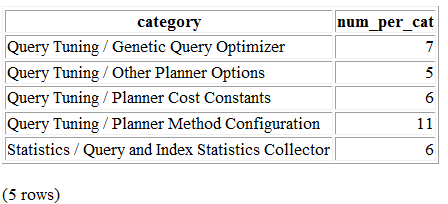
Not too shabby. But the command outputs only an HTML table, not a fully qualified HTML document. To create a meatier report, compose a script, as shown in Example 3-14.
\o settings_report.htmlFROM pg_settings WHERE category LIKE '%Planner%' GROUP BY category ORDER BY category; \H \qecho '</td><td><h2>File Locations</h2>' \x off
\t on \pset format html SELECT name, setting FROM pg_settings WHERE category = 'File Locations' ORDER BY name; \qecho '<h2>Memory Settings</h2>' SELECT name, setting, unit FROM pg_settings WHERE category ILIKE '%memory%' ORDER BY name; \qecho '</td></tr></table>' \qecho '</body></html>' \o
Redirects query output to a file.
CSS table settings for query output.
Appends additional HTML.
Expand mode. Repeats the column headers for each row and outputs each column of each row as a separate row.
Forces the queries to output as an HTML table.
string_agg(), introduced in PostgreSQL 9.0, concatenates all
properties in the same category into a single column.
Turns off expand mode. The second and third queries should output one row per table row.
Toggles tuples mode. When on, column headers and row counts are omitted.
Example 3-14 demonstrates that by
interspersing SQL and psql commands, you can create a comprehensive
tabular report replete with subreports. Run Example 3-14 by connecting interactively with
psql and executing \i settings_report.psql. Alternatively,
run psql noninteractively by executing psql -f
settings_report.psql from your OS command line. The output
generated by settings_report.html is
shown in Figure 3-2.
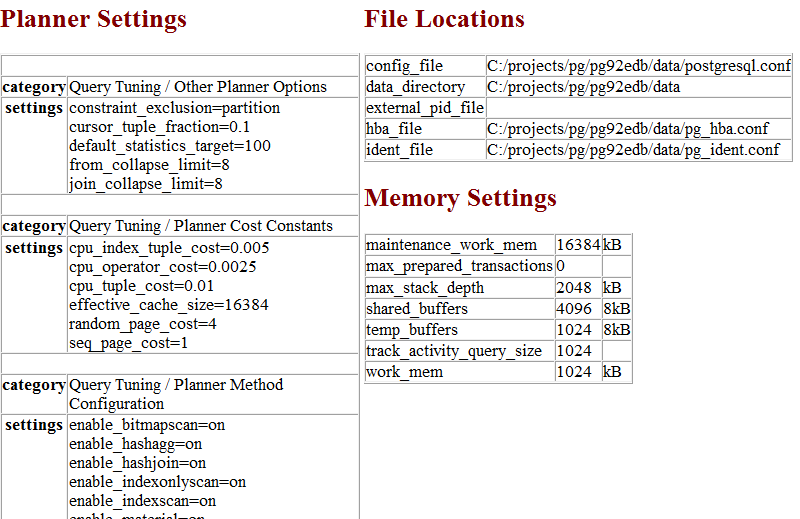
As demonstrated, composing psql scripts lets you show output from many queries within a single report. Further, after you write a script, you can schedule its execution in the future, and at fixed intervals. Use a daemon like pgAgent, crontab, or Windows Scheduler.
pgAdmin4 version 1.6 is the current rendition of the tried-and-true graphical administration tool for PostgreSQL. It is a complete rewrite of the predecessor pgAdmin3. Some features of pgAdmin3 have not been ported to pgAdmin4, though they may be in the future. In this chapter we’ll focus on what’s available in pgAdmin4. Much of the functionality you will find in pgAdmin4 was present in pgAdmin3, so this discussion will be valuable even if you are still using pgAdmin3. We will also cover some popular features of pgAdmin3 not yet ported to pgAdmin4. For the rest of this chapter, we’ll simply refer to both as pgAdmin, and only make distinguishing version notes where the functionality is different.
Most of the key changes thus far with pgAdmin4 compared to pgAdmin3 is that pgAdmin4 better supports the new 9.6 and 10 constructs including the ability to run in a server or desktop mode; an improved query results pane with ability to edit records and also select noncontiguous rows; and improved performance. If you are using Windows, make sure to use pgAdmin4 1.6 or above. Prior pgAdmin4 versions had performance issues on Windows when running in desktop mode.
Although pgAdmin has shortcomings, we are always encouraged by not only how quickly bugs are fixed, but also how quickly new features are added. Because the PostgreSQL developers position pgAdmin as the most commonly used graphical-administration tool for PostgreSQL and it is packaged with many binary distributions of PostgreSQL, the developers have taken on the responsibility of keeping pgAdmin always in sync with the latest PostgreSQL releases. If a new release of PostgreSQL introduces new features, you can count on the latest pgAdmin to let you manage it. If you’re new to PostgreSQL, you should definitely start with pgAdmin before exploring other tools.
pgAdmin4 comes packaged with many distributions. The BigSQL and EDB distributions from PostgreSQL 9.6 on include pgAdmin4 as an option. Note if you have a need for pgAdmin3 for PostgreSQL 9.6+, you’ll want to use the BigSQL pgAdmin3 LTS, which has been patched to handle versions 9.6 and 10. pgAdmin3 LTS is installable via the BigSQL package manager. After version 9.5, the EDB package only includes pgAdmin4. The pgAdmin group will no longer be making updates or enhancements to pgAdmin3.
If you are installing pgAdmin without PostgreSQL, you can download pgAdmin from pgadmin.org. While on the site, you can opt to peruse one of the guides introducing pgAdmin. The tool is well-organized and, for the most part, guides itself quite well. Adventurous users can always try beta and alpha releases of pgAdmin. Your help in testing would be greatly appreciated by the PostgreSQL community.
To whet your appetite, here’s a list of our favorite goodies in pgAdmin. More are listed in pgAdmin Features:
pgAdmin4 can be installed in desktop mode or as a web server WSGI application. pgAdmin3 was a desktop-only application.
This awesome feature offers pictorial insight into what the query planner is thinking. While verbose text-based planner output still has its place, a graphical explain provides a more digestible bird’s-eye view.
pgAdmin ultimately interacts with PostgreSQL via SQL, and it’s not shy about letting you see the generated SQL. When you use the graphical interface to make changes to your database, pgAdmin automatically displays, in an SQL pane, the underlying SQL that will perform the tasks. For novices, studying the generated SQL is a superb learning opportunity. For pros, taking advantage of the generated SQL is a great timesaver.
You no longer need to dig around for the files and use
another editor. This is currently only present in pgAdmin3, and to
use it, you also need to install the pgadmin extension in the database called
postgres.
pgAdmin can easily export query results as a CSV file or other delimited format and import such files as well. pgAdmin3 can even export results as HTML, providing you with a turnkey reporting engine, albeit a bit crude.
Can’t remember the myriad commands and switches to perform a backup or restore using pg_restore and pg_dump? pgAdmin has a nice interface that lets you selectively back up and restore databases, schemas, single tables, and globals. You can view and copy the underlying pg_dump or pg_restore command that pgAdmin used in the Message tab.
This timesaver allows you to change privileges on many database objects in one fell swoop.
This is a quick-and-dirty way to run scripts that don’t have to complete as transactions. With this you can execute loops that commit on each iteration, unlike functions that require all steps to be completed before the work is committed. Unfortunately, you cannot use this engine outside of pgAdmin and it is currently only available in pgAdmin3 (not 4).
To trigger the autocomplete popup use CTRL-Space. The autocomplete feature is improved in pgAdmin4.
We’ll devote an entire section to this cross-platform job scheduling agent. pgAdmin provides a cool interface to it.
Connecting to a PostgreSQL server with pgAdmin is straightforward. The General and Connection tabs are shown in Figure 4-1.
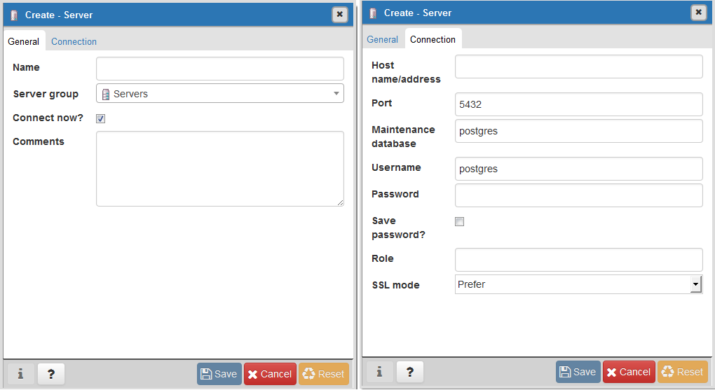
The tree layout of pgAdmin is intuitive to follow but does engender some possible anxiety, because it starts off by showing you every esoteric object found in the database. You can pare down the tree display by going into the Browser section of Preferences and deselecting objects that you would rather not have to stare at every time you use pgAdmin. To declutter the browse tree sections, go to Files→Preferences→Browser→Nodes. You will see the screen shown in Figure 4-2.
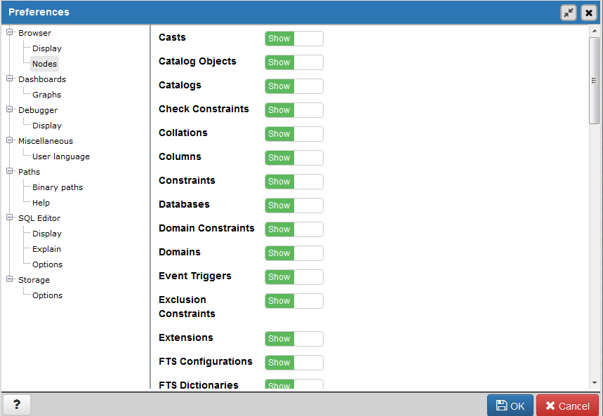
If you select Show System Objects in the Display section, you’ll
see the guts of your server: internal functions, system tables, hidden
columns in tables, and so forth. You will also see the metadata stored
in the PostgreSQL system catalogs: information_schema catalog and the pg_catalog. information_schema is an ANSI SQL standard
catalog found in other databases such as MySQL and SQL Server. You may
recognize some of the tables and columns from working with other
database products.
pgAdmin is chock full of goodies. We don’t have the space to bring them all to light, so we’ll just highlight the features that many use on a regular basis.
pgAdmin has this menu option that will autogenerate a template for SELECT, INSERT, and UPDATE statements from a table definition. You access this feature by right-clicking the table and accessing the SCRIPTS context menu option as shown in Figure 4-3.
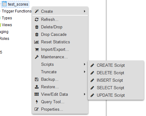
The “SELECT Script” option is particularly handy because it will create a query that lists all the columns in the table. If you have a lot of columns in a table and want to select a large subset but not all columns, this is a great timesaver. You can remove columns you don’t need in your query from the autogenerated statement.
Although pgAdmin is a great tool, psql does a better job in a few cases. One of them is the
execution of very large SQL files, such as those created by pg_dump and other dump tools. You can easily
jump to psql from pgAdmin3, but this feature is not available in
pgAdmin4. Click the plugin menu, as shown in Figure 4-4, and then click PSQL Console. This
opens a psql session connected to the database you are currently
connected to in pgAdmin. You can then use the \cd and \i commands
to change directory and run the SQL file.
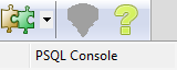
Because this feature relies on a database connection, you’ll see it disabled until you’re connected to a database.
You can edit configuration files directly from pgAdmin, provided that you installed the adminpack extension on your server. PostgreSQL one-click installers generally create the adminpack extension. If it’s present, you should see the Server Configuration menu enabled, as shown in Figure 4-5.
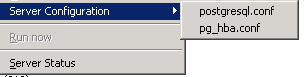
If the menu is grayed out and you are connected to a PostgreSQL
server, either you don’t have the adminpack installed on that server or you are not logged in as a
superuser. To install the adminpack run the SQL statement CREATE EXTENSION adminpack; or use
the graphical interface for installing extensions, as shown in Figure 4-6. Disconnect from the server
and reconnect; you should see the menu enabled.
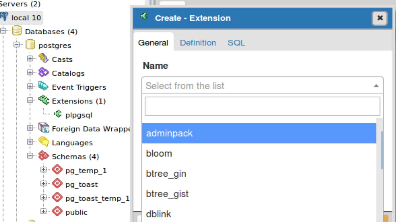
pgAdmin lets you create all kinds of database assets and assign privileges.
Creating a new database in pgAdmin is easy. Just right-click the database section of the tree and choose New Database, as shown in Figure 4-7. The Definition tab provides a drop-down menu for you to select a template database, similar to what we did in “Template Databases”.
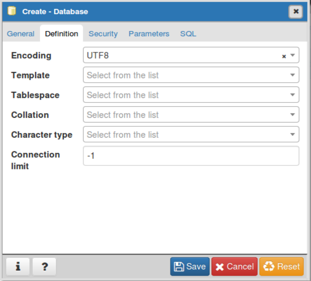
Follow the same steps to create roles, schemas, and other objects. Each will have its own relevant set of tabs for you to specify additional attributes.
To manage the privileges of database assets, nothing beats the
pgAdmin Grant Wizard, which you access from the Tools→Grant
Wizard menu of pgAdmin. If you are interested in granting permissions
only for objects in a specific schema, right-click the schema and
choose “Grant Wizard.” The list will be filtered to just objects in
the schema. As with many other features, this option is grayed out
unless you are connected to a database. It’s also sensitive to the
location in the tree you are on. For example, to set privileges for
items in the census schema, select
the schema and then choose Grant Wizard. The Grant Wizard screen is
shown in Figure 4-8. You can then
select all or some of the items and switch to the Privileges tab to
set the roles and privileges you want to grant.
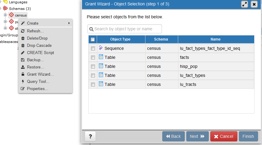
More often than setting privileges on existing objects, you may want to set default privileges for new objects in a schema or database. To do so, right-click the schema or database, select Properties, and then go to the Default Privileges tab, as shown in Figure 4-9.
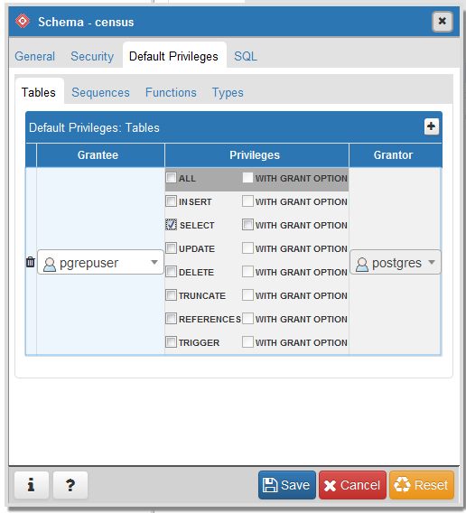
When setting privileges for a schema, make sure to also set the usage privilege on the schema to the groups you will be giving access to.
Like psql, pgAdmin allows you to import and export text files.
The import/export feature is really a wrapper around the
psql \copy command and requires the table
that will receive the data to exist already. In order to import data,
right-click the table you want to import/export data to. Figure 4-10 shows the menu that comes up
after we right-click the lu_fact_types table on the
left.
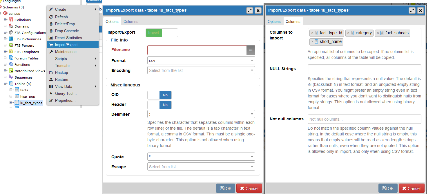
In addition to importing data, you can export your queries as well. pgAdmin3 allows exporting to delimited CSV, HTML, or XML formats. The pgAdmin4 export feature is much simpler and basic than pgAdmin3.
In pgAdmin to export with delimiters, perform the following:
Open the query window (![]() ).
).
Write the query.
Run the query.
In pgAdmin3, you’d choose File→Export. In pgAdmin4, you
click the download icon (![]() ) and browse to where you want to
save.
) and browse to where you want to
save.
For pgAdmin3, you get additional prompts before being given a save option. Fill out the settings as shown in Figure 4-11.
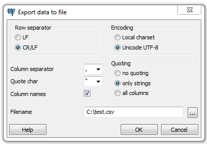
Exporting as HTML or XML is much the same, except you use the File→Quick Report option (see Figure 4-12).
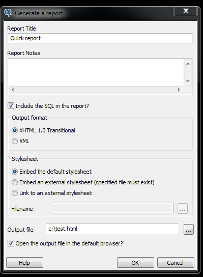
pgAdmin offers a graphical interface to pg_dump and
pg_restore, covered in “Backup and Restore”. In this section, we’ll repeat some of the same
examples using pgAdmin instead of the command line.
If several versions of PostgreSQL or pgAdmin are installed on your computer, it’s a good idea to make sure that the pgAdmin version is using the versions of the utilities that you expect. Check what the bin setting in pgAdmin is pointing to in order to ensure it’s the latest available, as shown in Figure 4-13.
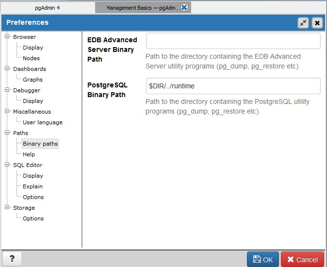
If your server is remote or your databases are huge, we
recommend using the command-line tools for backup and restore instead
of pgAdmin to avoid adding another layer of complexity to what could already be a pretty lengthy process. Also
keep in mind that if you do a compressed/TAR/directory backup with a
newer version of pg_dump, you need
to use the same or later version of pg_restore.
In “Selective Backup Using pg_dump”, we demonstrated how to back up a database. To repeat the same steps using the pgAdmin interface, right-click the database you want to back up and choose Custom for Format, as shown in Figure 4-14.
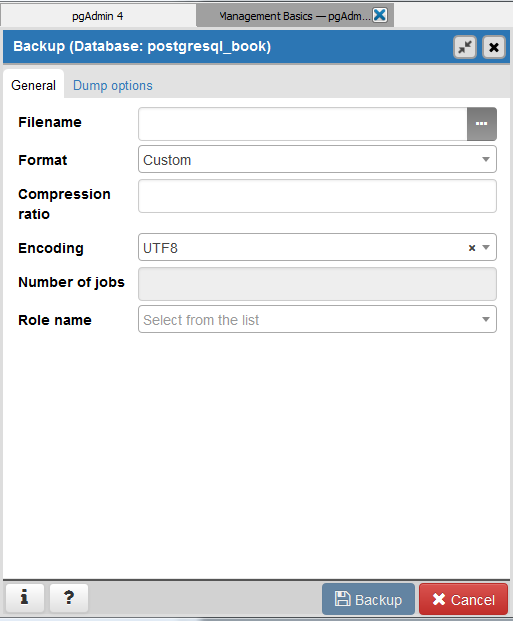
pgAdmin provides a graphical interface to pg_dumpall for backing up system objects. To use the interface, first
connect to the server you want to back up. Then, from the top menu,
choose Tools→Backup Globals.
pgAdmin doesn’t give you control over which global objects to back up, as the command-line interface does. pgAdmin backs up all tablespaces and roles.
If you ever want to back up the entire server, invoke pg_dumpall by going to the top menu and
choosing Tools→Backup Server.
pgAdmin provides a graphical interface to pg_dump for selective backup. Right-click
the asset you want to back up and select Backup (see Figure 4-15). You can back up an entire
database, a particular schema, a table, or anything else.
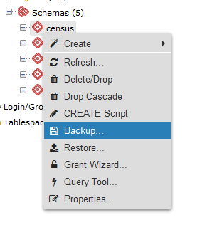
To back up the selected asset, you can forgo the other tabs (see Figure 4-14). In pgAdmin3, you can selectively drill down to more items by clicking the Objects tab, as shown in Figure 4-16. This feature is not yet present in pgAdmin4.
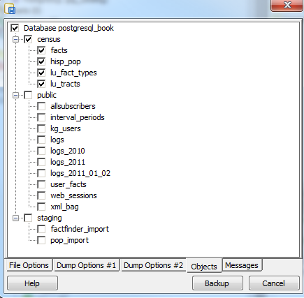
pgScript is a built-in scripting tool in pgAdmin3 but is not present in pgAdmin4. It’s most useful for running repetitive SQL tasks. pgScript can make better use of memory, and thus be more efficient, than equivalent PostgreSQL functions. This is because stored functions maintain all their work in memory and commit all the results of a function in a single batch. In contrast, pgScript commits each SQL insert or update statement as it runs through the script. This makes pgScript particularly handy for memory-hungry processes that you don’t need completed as single transactions. After each transaction commits, memory becomes available for the next one. You can see an example where we use pgScript for batch geocoding at Using pgScript for Geocoding.
The pgScript language is lazily typed and supports conditionals,
loops, data generators, basic print statements, and record variables. The
general syntax is similar to that of Transact SQL, the stored procedure
language of Microsoft SQL Server. Variables, prepended with
@, can hold scalars or arrays, including the results of SQL
commands. Commands such as DECLARE and SET, and
control constructs such as IF-ELSE and WHILE
loops, are part of the pgScript language.
Launch pgScript by opening a regular SQL query window. After typing
in your script, execute it by clicking the pgScript icon
(![]() ).
).
We’ll now show you some examples of pgScripts. Example 4-1 demonstrates how to use
pgScript record variables and loops to build a crosstab table, using the lu_fact_types table we create
in Example 7-22. The pgScript
creates an empty table called census.hisp_pop with numeric
columns: hispanic_or_latino, white_alone,
black_or_african_american_alone, and so on.
DECLARE @I, @labels, @tdef; SET @I = 0;Labels will hold records.SET @labels = SELECT quote_ident( replace( replace(lower(COALESCE(fact_subcats[4], fact_subcats[3])), ' ', '_') ,':','' ) ) As col_name, fact_type_id FROM census.lu_fact_types WHERE category = 'Population' AND fact_subcats[3] ILIKE 'Hispanic or Latino%' ORDER BY short_name; SET @tdef = 'census.hisp_pop(tract_id varchar(11) PRIMARY KEY ';Loop through records using LINES function.WHILE @I < LINES(@labels) BEGIN SET @tdef = @tdef + ', ' + @labels[@I][0] + ' numeric(12,3) '; SET @I = @I + 1; END SET @tdef = @tdef + ')';Print out table def.PRINT @tdef;create the table.CREATE TABLE @tdef;
Although pgScript does not have an execute command that allows you
to run dynamically generated SQL, we accomplished the same thing in Example 4-1 by assigning an SQL string to a
variable. Example 4-2 pushes
the envelope a bit further by populating the census.hisp_pop table we
just created.
DECLARE@I,@labels,@tload,@tcols,@fact_types;SET@I=0;SET@labels=SELECTquote_ident(replace(replace(lower(COALESCE(fact_subcats[4],fact_subcats[3])),' ','_'),':',''))Ascol_name,fact_type_idFROMcensus.lu_fact_typesWHEREcategory='Population'ANDfact_subcats[3]ILIKE'Hispanic or Latino%'ORDERBYshort_name;SET@tload='tract_id';SET@tcols='tract_id';SET@fact_types='-1';WHILE@I<LINES(@labels)BEGINSET@tcols=@tcols+', '+@labels[@I][0];SET@tload=@tload+', MAX(CASE WHEN fact_type_id = '+CAST(@labels[@I][1]ASSTRING)+' THEN val ELSE NULL END)';SET@fact_types=@fact_types+', '+CAST(@labels[@I][1]AsSTRING);SET@I=@I+1;ENDINSERTINTOcensus.hisp_pop(@tcols)SELECT@tloadFROMcensus.factsWHEREfact_type_idIN(@fact_types)ANDyr=2010GROUPBYtract_id;
The lesson to take away from Example 4-2 is that you can dynamically append SQL fragments into a variable.
One of the great gems in pgAdmin is its at-a-glance graphical explain of the query plan. You
can access the graphical explain plan by opening up an SQL query window,
writing a query, and clicking the explain icon (![]() ).
).
Suppose we run the query:
SELECTleft(tract_id,5)Ascounty_code,SUM(hispanic_or_latino)Astot,SUM(white_alone)Astot_white,SUM(COALESCE(hispanic_or_latino,0)-COALESCE(white_alone,0))ASnon_whiteFROMcensus.hisp_popGROUPBYcounty_codeORDERBYcounty_code;
We will get the graphical explain shown in Figure 4-17. Here’s a quick tip for interpreting the graphical explain: trim the fat! The fatter the arrow, the longer a step takes to complete.
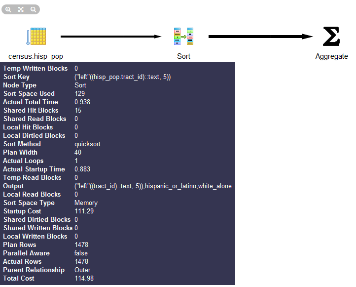
Graphical explain is disabled if Query→Explain→Buffers is enabled. So make sure to uncheck buffers before trying a graphical explain. In addition to the graphical explain, the Data Output tab shows the textual explain plan, which for this example looks like:
GroupAggregate  (cost=111.29..151.93 rows=1478 width=20)
  Output: ("left"((tract_id)::text, 5)), sum(hispanic_or_latino),
sum(white_alone), ...
  ->  Sort  (cost=111.29..114.98 rows=1478 width=20)
     Output: tract_id, hispanic_or_latino, white_alone,
     ("left"((tract_id)::text, 5))
	Sort Key: ("left"((tract_id)::text, 5))
	->  Seq Scan on census.hisp_pop  (cost=0.00..33.48 rows=1478 width=20)
		  Output: tract_id, hispanic_or_latino
, white_alone, "left"((tract_id)::text, 5)pgAgent is a handy utility for scheduling PostgreSQL jobs. But it can also execute batch scripts on the OS, replacing
crontab on Linux/Unix and the Task Scheduler on Windows. pgAgent goes even
further: you can schedule jobs to run on any other host regardless of OS.
All you have to do is install the pgAgent service on the host and point it
to use a specific PostgreSQL database with pgAgent tables and functions
installed. The PostgreSQL server itself is not required, but the client
connection libraries are. Because pgAgent is built atop PostgreSQL, you
are blessed with the added advantage of having access to all the tables
controlling the agent. If you ever need to replicate a complicated job
multiple times, you can go straight into the database tables directly and
insert the records for new jobs, skipping the pgAdmin interface.
We’ll get you started with pgAgent in this section. Visit Setting Up pgAgent and Doing Scheduled Backups to see more working examples and details on how to set it up.
You can download pgAgent from pgAgent
Download. It is also available via the EDB Application
Stackbuilder and BigSQL package. The packaged extension script creates a
new schema named pgAgent in the postgres database. When you connect to your
server via pgAdmin, you will see a new section called Jobs, as shown in
Figure 4-18.
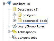
Although pgAgent is installed by default in postgres db, you can
install in a different database using CREATE EXTENSION pgagent;. If you
decide to install in a different database, make sure to set your
pgagent service to use that database and in pgAdmin set the
maintenance db in the server connection tab to be this
database.
If you want pgAgent to run batch jobs on additional servers, follow the same steps, except that you don’t have to reinstall the SQL script packaged with pgAgent. Pay particular attention to the OS permission settings of the pgAgent service/daemon account. Make sure each agent has sufficient privileges to execute the batch jobs that you will be scheduling.
Batch jobs often fail in pgAgent even when they might run fine from the command line. This is often due to permission issues. pgAgent always runs under the same account as the pgAgent service/daemon. If this account doesn’t have sufficient privileges or the necessary network path mappings, jobs fail.
Each scheduled job has two parts: the execution steps and the schedule. When creating a new job, start by adding one or more job steps. Figure 4-19 shows what the step add/edit screen looks like.
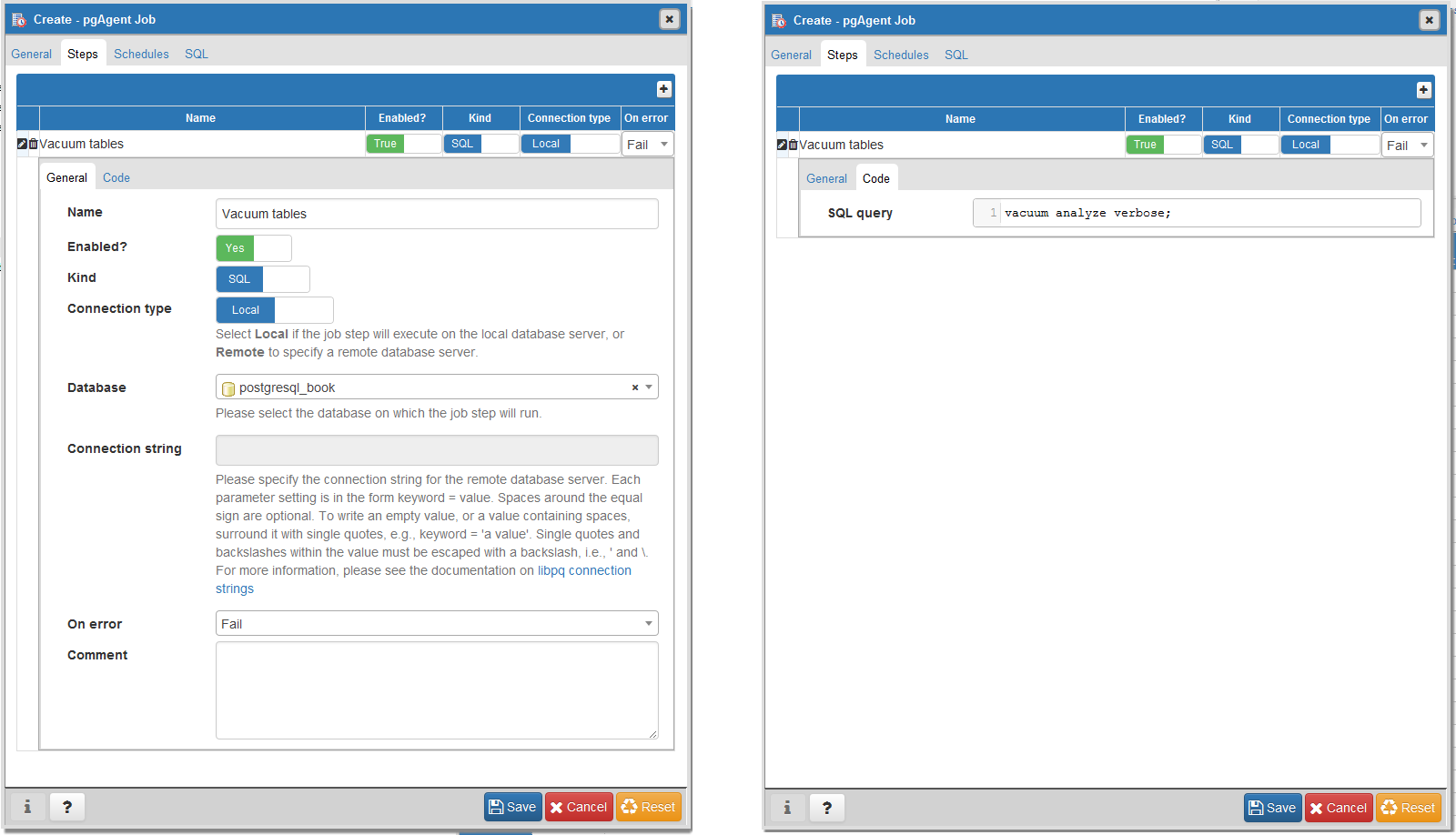
For each step, you can enter an SQL statement to run, point to a shell script on the OS, or even cut and paste in a full shell script as we commonly do.
If you choose SQL, the connection type option becomes enabled and defaults to local. With a local connection, the job step runs on the same server as the pgAgent and uses the same authentication username and password. You need to additionally specify the database that pgAgent should connect to in order to run the jobs. The screen offers you a drop-down list of databases to choose from. If you choose a remote connection type, the text box for entering a connection string becomes enabled. Type in the full connection string, including credentials and the database. When you connect to a remote PostgreSQL server with an earlier version of PostgreSQL, make sure that all the SQL constructs you use are supported on that version.
If you choose to run batch jobs, the syntax must be specific to the OS running the job. For example, if your pgAgent is running on Windows, your batch jobs should have valid DOS commands. If you are on Linux, your batch jobs should have valid shell or Bash commands.
Steps run in alphabetical order, and you can decide what kinds of actions you want to take upon success or failure of each step. You have the option of disabling steps that should remain dormant but that you don’t want to delete because you might reactivate them later.
Once you have the steps ready, go ahead and set up a schedule to run them. You can set up intricate schedules with the scheduling screen. You can even set up multiple schedules.
If you installed pgAgent on multiple servers and have them all pointing to the same pgAgent database, all these agents by default will execute all jobs.
If you want to run the job on just one specific machine, fill in
the host agent field when creating the job. Agents
running on other servers will skip the job if it doesn’t match their
hostname.
pgAgent consists of two parts: the data defining the jobs and
the logging of the job. Log information resides in the pgAgent schema,
usually in the postgres database; the job agents
query the jobs for the next job to run and then insert relevant
logging information in the database. Generally, both the PostgreSQL
server holding the data and the job agent executing the jobs reside on
the same server, but they are not required to. Additionally, a single
PostgreSQL server can service many job agents residing on different
servers.
A fully formed job is shown in Figure 4-20.
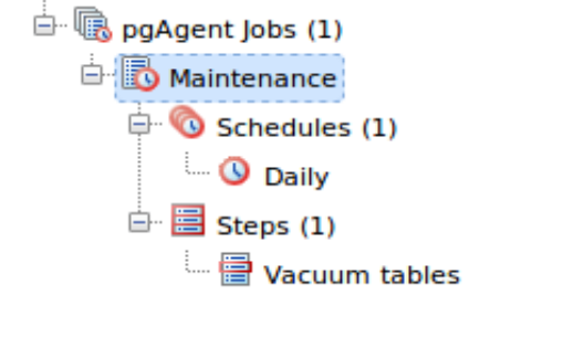
With your finely honed SQL skills, you can easily replicate jobs, delete jobs,
and edit jobs directly by messing with pgAgent metatables. Just be
careful! For example, to get a glimpse inside the tables controlling all
of your agents and jobs, connect to the postgres database and execute the query in
Example 4-3.
SELECTc.relnameAstable_name,d.descriptionFROMpg_classAscINNERJOINpg_namespacenONn.oid=c.relnamespaceINNERJOINpg_descriptionAsdONd.objoid=c.oidANDd.objsubid=0WHEREn.nspname='pgagent'ORDERBYc.relname;
table_name     |       description
---------------+-------------------------
pga_job        | Job main entry
pga_jobagent   | Active job agents
pga_jobclass   | Job classification
pga_joblog     | Job run logs.
pga_jobstep    | Job step to be executed
pga_jobsteplog | Job step run logs.
pga_schedule   | Job schedule exceptions
Although pgAdmin already provides an intuitive interface to pgAgent scheduling and logging, you may find the need to generate your own job reports. This is especially true if you have many jobs or you want to compile stats from your job results. Example 4-4 demonstrates the one query we use often.
SELECTj.jobname,s.jstname,l.jslstart,l.jslduration,l.jsloutputFROMpgagent.pga_jobsteplogAslINNERJOINpgagent.pga_jobstepAssONs.jstid=l.jsljstidINNERJOINpgagent.pga_jobAsjONj.jobid=s.jstjobidWHEREjslstart>CURRENT_DATEORDERBYj.jobname,s.jstname,l.jslstartDESC;
We find this query essential for monitoring batch jobs because
sometimes a job will report success even though it failed. pgAgent can’t
always discern the success or failure of a shell script on the OS. The
jsloutput field in the logs provides
the shell output, which usually details what went wrong.
PostgreSQL supports the workhorse data types of any database: numerics, strings, dates, times, and booleans. But PostgreSQL sprints ahead by adding support for arrays, time zone−aware datetimes, time intervals, ranges, JSON, XML, and many more. If that’s not enough, you can invent custom types. In this chapter, we don’t intend to cover every data type. For that, there’s always the manual. We showcase data types that are unique to PostgreSQL and nuances in how PostgreSQL handles common data types.
No data type would be useful without a cast of supporting functions and operators. And PostgreSQL has plenty of them. We’ll cover the more popular ones in this chapter.
When we use the term function, we’re talking about something that’s of the form
f(x). When we use the term operator,
we’re talking about something that’s symbolic and either unary
(having one argument) or binary (having two arguments) such as
+, -, *, or /. When
using operators, keep in mind that the same symbol can take on a different
meaning when applied to different data types. For example, the plus sign
means adding for numerics but unioning for ranges.
You will find your everyday integers, decimals, and floating-point numbers in PostgreSQL. Of the numeric types, we want to discuss serial data types and a nifty function to quickly generate arithmetic series of integers.
Serial and its bigger sibling, bigserial, are auto-incrementing
integers often used as primary keys of tables in which a natural key is not
apparent. This data type goes by different names in different database
products, with autonumber being the most common
alternative moniker. When you create a table and specify a column as
serial, PostgreSQL first creates an integer column and then creates a
sequence object named
table_name_column_name_seq
In PostgreSQL, the sequence type is a database asset in its own
right. You can inspect and edit the sequences using SQL with the ALTER SEQUENCE command or using PGAdmin.
You can set the current value, boundary values (both the upper and lower
bounds), and even how many numbers to increment each time. Though
decrementing is rare, you can do it by setting the increment value to a
negative number. Because sequences are independent database assets, you
can create them separately from a table using the CREATE
SEQUENCE command, and you can use the same sequence
across multiple tables. The cross-table sharing of the same sequence
comes in handy when you’re assigning a universal key in your
database.
To use an extant sequence for subsequent tables, create a new
column in the table as integer or bigint—not as serial—then set the default value
of the column using the nextval(
function as shown in Example 5-1.sequence_name)
CREATESEQUENCEsSTART1;CREATETABLEstuff(idbigintDEFAULTnextval('s')PRIMARYKEY,nametext);
If you rename a table that has a serial based on a sequence, PostgreSQL will not automatically rename the sequence object. To avoid confusion, you should rename the sequence object.
PostgreSQL has a nifty function called generate_series not
found in other database products. The function comes in two forms. One
is a numeric version that creates a sequence of integers incremented by
some value and one that creates a sequence of dates or timestamps
incremented by some time interval. What makes
generate_series so convenient is that it allows you to
effectively mimic a for loop in SQL. Example 5-2 demonstrates the numeric
version. Example 5-13 demonstrates
the temporal version.
Example 5-2 uses integers with an optional step parameter.
SELECTxFROMgenerate_series(1,51,13)Asx;
x
----
1
14
27
40
The default step is 1. As demonstrated in Example 5-2, you can pass in an optional step argument to specify how many steps to skip for each successive element. The end value will never exceed our prescribed range, so although our range ends at 51, our last number is 40 because adding another 13 to our 40 busts the upper bound.
There are three primitive textual types in PostgreSQL: character (abbreviable as char),
character varying (abbreviable as varchar), and text.
Use char only when the values stored are fixed length, such as postal codes, phone numbers, and Social Security numbers in the US. If your value is under the length specified, PostgreSQL automatically adds spaces to the end. When compared with varchar or text, the right-padding takes up more superfluous storage, but you get the assurance of an invariable length. There is absolutely no speed performance benefit of using char over varchar or text and char will always take up more disk space. Use character varying to store strings with varying length. When defining varchar columns, you should specify the maximum length of a varchar. Text is the most generic of the textual data types. With text, you cannot specify a maximum length.
The max length modifier for varchar is optional. Without it, varchar
behaves almost identically to text. Subtle differences do surface when
connecting to PostgreSQL via drivers. For instance, the ODBC driver cannot
sort text columns. Both varchar and text have a maximum storage of 1G for
each value—that’s a lot! Behind the scenes, any value larger than what can
fit in a record page gets pushed to TOAST.
Some folks advocate abandoning varchar and always using text. Rather than waste space arguing about it here, read the debate at In Defense of Varchar(X).
Often, for cross-system compatibility, you want to remove case sensitivity from your character types. To do this, you need to override comparison operators that take case into consideration. Overriding operators is easier for varchar than it is for text. We demonstrate an example in Using MS Access with PostgreSQL, where we show how to make varchar behave without case sensitivity and still be able to use an index.
Common string manipulations are padding (lpad, rpad), trimming
whitespace (rtrim, ltrim,
trim, btrim), extracting substrings (substring), and concatenating (||). Example 5-3 demonstrates padding, and Example 5-4 demonstrates trimming.
SELECTlpad('ab',4,'0')Asab_lpad,rpad('ab',4,'0')Asab_rpad,lpad('abcde',4,'0')Asab_lpad_trunc;
ab_lpad | ab_rpad | ab_lpad_trunc
--------+---------+---------------
00ab    | ab00    | abcd
lpad truncates instead of padding if the string
is too long.
By default, trim functions remove spaces, but you can pass in an optional argument indicating other characters to trim.
SELECTaAsa_before,trim(a)Asa_trim,rtrim(a)Asa_rt,iAsi_before,ltrim(i,'0')Asi_lt_0,rtrim(i,'0')Asi_rt_0,trim(i,'0')Asi_t_0FROM(SELECTrepeat(' ',4)||i||repeat(' ',4)Asa,'0'||iAsiFROMgenerate_series(0,200,50)Asi)Asx;
a_before | a_trim | a_rt | i_before | i_lt_0 | i_rt_0 | i_t_0
---------+--------+------+----------+--------+--------+------
0        | 0      | 0    | 00       |        |        |
50       | 50     | 50   | 050      | 50     | 05     | 5
100      | 100    | 100  | 0100     | 100    | 01     | 1
150      | 150    | 150  | 0150     | 150    | 015    | 15
200      | 200    | 200  | 0200     | 200    | 02     | 2
A helpful function for aggregating strings is the string_agg function, which we demonstrate in Examples 3-14 and 5-26.
There are a couple of useful functions in PostgreSQL for tearing strings apart.
The split_part function is useful for extracting an element from a delimited
string, as shown in Example 5-5. Here, we
select the second item in a string of items delimited by periods.
SELECTsplit_part('abc.123.z45','.',2)Asx;
x
---
123
The string_to_array function is useful for creating an array of elements from a delimited
string. By combining string_to_array with the
unnest function, you can expand the returned array into a set of rows, as
shown in Example 5-6.
SELECTunnest(string_to_array('abc.123.z45','.'))Asx;
x
---
abc
123
z45
PostgreSQL’s regular expression support is downright fantastic. You can return matches as tables or arrays and choreograph replaces and updates. Back-referencing and other fairly advanced search patterns are also supported. In this section, we’ll provide a small sampling. For more information, see Pattern Matching and String Functions.
Example 5-7 shows you how to format phone numbers stored simply as contiguous digits.
SELECTregexp_replace('6197306254','([0-9]{3})([0-9]{3})([0-9]{4})',E'\(\\1\) \\2-\\3')Asx;
x
--------------
(619) 730-6254
The \\1, \\2, etc., refer to elements in
our pattern expression. We use a backslash (\) to escape the parentheses.
The E' construct is PostgreSQL syntax for denoting that the
string to follow should be taken literally.
Suppose some field contains text with embedded phone numbers; Example 5-8 shows how to extract the phone numbers and turn them into rows all in one step.
SELECTunnest(regexp_matches('Cell (619) 852-5083. Work (619)123-4567 , Casa 619-730-6254. Bésame mucho.',E'[(]{0,1}[0-9]{3}[)-.]{0,1}[\\s]{0,1}[0-9]{3}[-.]{0,1}[0-9]{4}','g'))Asx;
x
--------------
(619) 852-5083
(619)123-4567
619-730-6254
(3 rows)
The matching rules for Example 5-8 are:
[(]{0,1}: starts with zero or one open
parenthesis.
[0-9]{3}: followed by three digits.
[)-.]{0,1}: followed by zero or one closed
parenthesis, hyphen, or period.
[\\s]+: followed by zero or more spaces.
[0-9]{4}: followed by four digits.
regexp_matches returns a string array consisting of matches of a regular
expression. The last input to our function is the flags
parameter. We set this to g, which stands for
global and returns all matches of a regular
expression as separate elements. If you leave out this
flags parameter, then your array will only contain the
first match. The flags parameter can consist of more
than one flag. For example, if you have letters in your regular
expression and text and you want to make the check case insensitive
and global, you would use two flags, gi. In addition to
the global flag, other allowed flags are listed in POSIX EMBEDDED OPTIONS.
There are many ways to compose the same regular expression. For
instance, \\d is shorthand for [0-9]. But
given the few characters you’d save, we prefer the more descriptive
longhand.
If you only care about the first match, you can utilize the
substring function, which will return the first matching
value as shown in Example 5-9.
SELECTsubstring('Cell (619) 852-5083. Work (619)123-4567 , Casa 619-730-6254. Bésame mucho.'fromE'[(]{0,1}[0-9]{3}[)-.]{0,1}[\\s]{0,1}[0-9]{3}[-.]{0,1}[0-9]{4}')Asx;
       x
----------------
 (619) 852-5083
(1 row)
In addition to the wealth of regular expression functions, you can
use regular expressions with the SIMILAR TO
(~) operators. The following example returns all description fields with
embedded phone numbers:
SELECT description
FROM mytable
WHERE description ~
E'[(]{0,1}[0-9]{3}[)-.]{0,1}[\\s]{0,1}[0-9]{3}[-.]{0,1}[0-9]{4}';PostgreSQL support for temporal data is second to none. In addition to the usual dates and
times types, PostgreSQL supports time zones, enabling the automatic
handling of daylight saving time (DST) conversions by region. Specialized data
types such as interval offer datetime arithmetic.
PostgreSQL also understands infinity and negative infinity, relieving us
from having to create conventions that we’ll surely forget. Range types provide support for
temporal ranges with a slew of companion operators,
functions, and indexes. We cover range types in “Range Types”.
At last count, PostgreSQL has nine temporal data types.
Understanding their distinctions is important in ensuring that you choose
the right data type for the job. All the types except range abide by ANSI SQL standards. Other leading
database products support some, but not all, of these data types. Oracle
has the most varieties of temporal types; SQL Server ranks second; and
MySQL comes in last.
PostgreSQL temporal types vary in a number of ways to handle different situations. If a type is time zone−aware, the time changes if you change your server’s time zone. The types are:
dateStores the month, day, and year, with no time zone awareness and no concept of hours, minutes, or seconds.
time (aka time without time
zone)Stores hours, minutes, and seconds with no awareness of time zone or calendar dates.
timestamp (aka timestamp without time
zone)Stores both calendar dates and time (hours, minutes, seconds) but does not care about the time zone.
timestamptz (aka timestamp with time
zone)A time zone−aware date and time data type. Internally,
timestamptz is stored in Coordinated Universal Time
(UTC), but its display defaults to the time zone of the server,
the service config, the database, the user, or the session. Yes, you
can observe different time zones at different levels. If you input a
timestamp with no time zone and cast it to one with the time zone,
PostgreSQL assumes the default time zone in effect. If you don’t set
your time zone in postgresql.conf, the server’s default
takes effect. This means that if you change your server’s time zone,
you’ll see all the displayed times change after the PostgreSQL
server restarts.
timetz (aka time with time
zone)The lesser-used sister of timestamptz. It is time zone−aware but
does not store the date. It always assumes DST of the current date
and time. Some programming languages with no concept of time without
date might map timetz to a timestamp with some
arbitrary date such as Unix Epoch 1970, resulting in year 1970 being
assumed.
intervalA duration of time in hours, days, months, minutes, and others. It comes in handy for datetime arithmetic. For example, if the world is supposed to end in exactly 666 days from now, all you have to do is add an interval of 666 days to the current time to get the exact moment (and plan accordingly).
tsrangeAllows you to define opened and closed ranges of timestamp with no timezone. The type
consists of two timestamps and opened/closed range qualifiers. For
example, '[2012-01-01 14:00, 2012-01-01
15:00)'::tsrange defines a period starting at 14:00 but
ending before 15:00. Refer to Range Types for details.
tstzrangeAllows you to define opened and closed ranges of timestamp with timezone.
daterangeA common misconception with PostgreSQL time zone−aware data types is that PostgreSQL
records an extra time marker with the datetime value itself. This is
incorrect. If you save 2012-2-14
18:08:00-8 (-8 being the Pacific offset from UTC), PostgreSQL
internally thinks like this:
Calculate the UTC time for 2012-02-14 18:08:00-8. This is 2012-02-15 04:08:00-0.
Store the value 2012-02-15
04:08:00.
When you call the data back for display, PostgreSQL internally works like this:
Start with the requested time zone, defaulting to the server time zone if none is requested.
Compute the offset for time zone for this UTC time (-5 for
America/New_York).
Determine the datetime with the offset (2012-02-15 16:08:00 with a -5 offset becomes 2012-02-15 21:08:00).
Display the result (2012-02-15
21:08:00-5).
So PostgreSQL doesn’t store the time zone, but uses it only to convert the datetime to UTC before storage. After that, the time zone information is discarded. When PostgreSQL displays datetime, it does so in the default time zone dictated by the session, user, database, or server, in that order. If you use time zone−aware data types, you should consider the consequence of a server move from one time zone to another. Suppose you based a server in New York City and subsequently restored the database in Los Angeles. All timestamps with time zone fields could suddenly display in Pacific time. This is fine as long as you anticipate this behavior.
Here’s an example of how something can go wrong. Suppose that
McDonald’s had its server on the East Coast and the opening time for
stores is stored as timetz. A new McDonald’s opens up in
San Francisco. The new franchisee phones McDonald’s headquarters to add
its store to the master directory with an opening time of 7 a.m. The
data entry dude entered the information as he is told: 7 a.m. The East
Coast PostgreSQL server interprets this to mean 7 a.m. Eastern, and now
early risers in San Francisco are lining up at the door wondering why
they can’t get their McBreakfasts at 4 a.m. Being hungry is one thing,
but we can imagine many situations in which confusion over a difference
of three hours could mean life or death.
Given the pitfalls, why would anyone want to use time zone−aware data types? First, it does spare you from having to do time zone conversions manually. For example, if a flight leaves Boston at 8 a.m. and arrives in Los Angeles at 11 a.m., and your server is in Europe, you don’t want to have to figure out the offset for each time manually. You could just enter the data with the Boston and Los Angeles local times. There’s another convincing reason to use time zone−aware data types: the automatic handling of DST. With countries deviating more and more from one another in DST schedules, manually keeping track of DST changes for a globally used database would require a dedicated programmer who does nothing but keep up-to-date with the latest DST schedules and map them to geographic enclaves.
Here’s an interesting example: a traveling salesperson catches a flight home from San Francisco to nearby Oakland. When she boards the plane, the clock at the terminal reads 2012-03-11 1:50 a.m. When she lands, the clock in the terminal reads 2012-03-11 3:10 a.m. How long was the flight? The key to the solution is that the change to DST occurred during the flight—the clocks sprang forward. With time zone−aware timestamps, you get 20 minutes, to which is a plausible answer for a short flight across the Bay. We get the wrong answer if we don’t use time zone−aware timestamps:
SELECT'2012-03-11 3:10 AM America/Los_Angeles'::timestamptz-'2012-03-11 1:50 AM America/Los_Angeles'::timestamptz;
gives you 20 minutes, whereas:
SELECT'2012-03-11 3:10 AM'::timestamp-'2012-03-11 1:50 AM'::timestamp;
gives you 1 hour and 20 minutes.
Let’s drive the point home with more examples, using a Boston server. For Example 5-10, I input my time in Los Angeles local time, but because my server is in Boston, I get a time returned in Boston local time. Note that it does give me the offset but that is merely display information. The timestamp is internally stored in UTC.
SELECT'2012-02-28 10:00 PM America/Los_Angeles'::timestamptz;
2012-02-29 01:00:00-05
In Example 5-11, we are getting back a timestamp without time zone. So the answer you get when you run this same query will be the same as mine, regardless of where in the world you are.
SELECT'2012-02-28 10:00 PM America/Los_Angeles'::timestamptzATTIMEZONE'Europe/Paris';
2012-02-29 07:00:00
The query is asking: what time is it in Paris if it’s 2012-02-28 10:00 p.m. in Los Angeles? Note the absence of the UTC offset in the result. Also, notice how you can specify a time zone with its official name rather than just an offset. Visit Wikipedia for a list of official time zone names.
The inclusion of a temporal interval data type greatly eases date and time arithmetic in PostgreSQL. Without it, we’d have to create another family of functions or use a nesting of functions as many other databases do. With intervals, we can add and subtract timestamp data simply by using the arithmetic operators we’re intimately familiar with. The following examples demonstrate operators and functions used with date and time data types.
The addition operator (+) adds an interval to
a timestamp:
SELECT'2012-02-10 11:00 PM'::timestamp+interval'1 hour';
2012-02-11 00:00:00
You can also add intervals:
SELECT'23 hours 20 minutes'::interval+'1 hour'::interval;
24:20:00
The subtraction operator (-) subtracts an interval from a temporal type:
SELECT'2012-02-10 11:00 PM'::timestamptz-interval'1 hour';
2012-02-10 22:00:00-05
OVERLAPS, demonstrated in Example 5-12, returns true if two temporal ranges overlap. This is
an ANSI SQL predicate equivalent to the overlaps function. OVERLAPS
takes four parameters, the first pair constituting one range and the
last pair constituting the other range. An overlap considers the time
periods to be half open, meaning that the start time is included but the
end time is outside the range. This is slightly different behavior from
the common BETWEEN predicate, which considers both start and end to be included. This
quirk won’t make a difference unless one of your ranges is a fixed point
in time (a period for which start and end are identical). Watch out for
this if you’re an avid user of the OVERLAPS function.
SELECT('2012-10-25 10:00 AM'::timestamp,'2012-10-25 2:00 PM'::timestamp)OVERLAPS('2012-10-25 11:00 AM'::timestamp,'2012-10-26 2:00 PM'::timestamp)ASx,('2012-10-25'::date,'2012-10-26'::date)OVERLAPS('2012-10-26'::date,'2012-10-27'::date)Asy;
x |y ---+--- t |f
In addition to operators and predicates, PostgreSQL comes with functions supporting temporal types. A full listing can be found at Datetime Functions and Operators. We’ll demonstrate a sampling here.
Once again, we start with the versatile
generate_series function. You can use this function with temporal types and interval
steps.
As you can see in Example 5-13, we can express dates in our local datetime format or the more global ISO yyyy-mm-dd format. PostgreSQL automatically interprets differing input formats. To be safe, we tend to stick with entering dates in ISO, because date formats vary from culture to culture, server to server, or even database to database.
SELECT(dt-interval'1 day')::dateAseomFROMgenerate_series('2/1/2012','6/30/2012',interval'1 month')Asdt;
eom ------------ 2012-01-31 2012-02-29 2012-03-31 2012-04-30 2012-05-31
Another popular activity is to extract or format parts of a
datetime value. Here, the functions date_part and to_char fit the
bill. Example 5-14 also
drives home the behavior of DST for a time zone−aware data type. We
intentionally chose a period that crosses a daylight saving switchover
in US/East. Because the clock springs
forward at 2 a.m., the final row of the table reflects the new
time.
SELECTdt,date_part('hour',dt)Ashr,to_char(dt,'HH12:MI AM')AsmnFROMgenerate_series('2012-03-11 12:30 AM','2012-03-11 3:00 AM',interval'15 minutes')Asdt;
dt | hr | mn -----------------------+----+---------- 2012-03-11 00:30:00-05 | 0 | 12:30 AM 2012-03-11 00:45:00-05 | 0 | 12:45 AM 2012-03-11 01:00:00-05 | 1 | 01:00 AM 2012-03-11 01:15:00-05 | 1 | 01:15 AM 2012-03-11 01:30:00-05 | 1 | 01:30 AM 2012-03-11 01:45:00-05 | 1 | 01:45 AM 2012-03-11 03:00:00-04 | 3 | 03:00 AM
By default, generate_series assumes
timestamptz if you don’t explicitly cast values to timestamp.
Arrays play an important role in PostgreSQL. They are particularly useful in building
aggregate functions, forming IN and ANY clauses,
and holding intermediary values for morphing to other data types. In
PostgreSQL, every data type has a companion array type. If you define your
own data type, PostgreSQL creates a corresponding array type in the
background for you. For example, integer has an integer array
type integer[], character has a character array
type character[], and so forth. We’ll show you some useful
functions to construct arrays short of typing them in manually. We will
then point out some handy functions for array manipulations. You can get
the complete listing of array functions and operators in the Official
Manual: Array Functions and Operators.
The most rudimentary way to create an array is to type the elements:
SELECTARRAY[2001,2002,2003]Asyrs;
If the elements of your array can be extracted from a query, you
can use the more sophisticated constructor function, array():
SELECTarray(SELECTDISTINCTdate_part('year',log_ts)FROMlogsORDERBYdate_part('year',log_ts));
Although the array function has to be used with a
query returning a single column, you can specify a composite type as the
output, thereby achieving multicolumn results. We demonstrate this in
“Custom and Composite Data Types”.
You can cast a string representation of an array to an array with syntax of the form:
SELECT'{Alex,Sonia}'::text[]Asname,'{46,43}'::smallint[]Asage;
name | age
-------------+--------
{Alex,Sonia} | {46,43}You can convert delimited strings to an array with the string_to_array function, as demonstrated
in Example 5-15.
SELECTstring_to_array('CA.MA.TX','.')Asestados;
estados
----------
{CA,MA,TX}
(1 row)array_agg is an aggregate function that can take a set of any data type
and convert it to an array, as demonstrated in Example 5-16.
SELECTarray_agg(log_tsORDERBYlog_ts)AsxFROMlogsWHERElog_tsBETWEEN'2011-01-01'::timestamptzAND'2011-01-15'::timestamptz;
x
------------------------------------------
{'2011-01-01', '2011-01-13', '2011-01-14'}PostgreSQL 9.5 introduced array_agg function support
for arrays. In prior versions if you wanted to aggregate rows of arrays
with array_agg, you’d get an error. array_agg support for arrays makes
it much easier to build multidimensional arrays from one-dimensional
arrays, as shown in Example 5-17.
SELECTarray_agg(f.t)FROM(VALUES('{Alex,Sonia}'::text[]),('{46,43}'::text[]))Asf(t);
array_agg
----------------------
{{Alex,Sonia},{46,43}}
(1 row)In order to aggregate arrays, they must be of the same data type and the same dimension. To force that in Example 5-17, we cast the ages to text. We also have the same number of items in the arrays being aggregated: two people and two ages. Arrays with the same number of elements are called balanced arrays.
A common function used with arrays is unnest, which allows you to expand
the elements of an array into a set of rows, as demonstrated in Example 5-18.
SELECTunnest('{XOX,OXO,XOX}'::char(3)[])Astic_tac_toe;
tic_tac_toe --- XOX OXO XOX
Although you can add multiple unnests to a single
SELECT, if the number of resultant rows from each array is
not balanced, you may get some head-scratching results.
A balanced unnest, as shown in Example 5-19, yields three rows.
SELECTunnest('{three,blind,mice}'::text[])Ast,unnest('{1,2,3}'::smallint[])Asi;
t |i ------+- three |1 blind |2 mice |3
If you remove an element of one array so that you don’t have an equal number of elements in both, you get the result shown in Example 5-20.
SELECTunnest('{blind,mouse}'::varchar[])ASv,unnest('{1,2,3}'::smallint[])ASi;
v |i ------+- blind |1 mouse |2 blind |3 mouse |1 blind |2 mouse |3
Version 9.4 introduced a multiargument unnest
function that puts in null placeholders where the arrays are not
balanced. The main drawback with the new unnest is that it can appear only in the
FROM clause. Example 5-21 revisits our unbalanced
arrays using the version 9.4 construct.
SELECT*FROMunnest('{blind,mouse}'::text[],'{1,2,3}'::int[])ASf(t,i);
t | i -------+--- blind | 1 mouse | 2 <NULL> | 3
PostgreSQL also supports array slicing using the
start:end syntax.
It returns another array that is a subarray of the original. For
example, to return new arrays that just contain elements 2 through 4 of
each original array, type:
SELECTfact_subcats[2:4]FROMcensus.lu_fact_types;
To glue two arrays together end to end, use the concatenation operator ||:
SELECTfact_subcats[1:2]||fact_subcats[3:4]FROMcensus.lu_fact_types;
You can also add additional elements to an existing array as follows:
SELECT'{1,2,3}'::integer[]||4||5;
The result is {1,2,3,4,5}.
Elements in arrays are most commonly referenced using the index of the element.
PostgreSQL array indexes start at 1. If you try to access an element
above the upper bound, you won’t get an error—only NULL will be returned. The next example grabs
the first and last element of our array column:
SELECTfact_subcats[1]ASprimero,fact_subcats[array_upper(fact_subcats,1)]AssegundoFROMcensus.lu_fact_types;
We used the array_upper function to get the upper bound of the array. The second required
parameter of the function indicates the dimension. In our case, our
array is one-dimensional, but PostgreSQL does support multidimensional
arrays.
PostgreSQL has several operators for working with array data. We already saw the
concatenation operator (||) for combining multiple arrays
into one or adding an element to an array in “Array Slicing and Splicing”. Arrays also support the
following comparison operators: =, <>,
<, >, @>,
<@, and &&. These operators require
both sides of the operator to be arrays of the same array data type. If
you have a GiST or GIN index on your array column, the comparison
operators can utilize them.
The overlap operator (&&) returns
true if two arrays have any elements in common. Example 5-22 will list all records in our table
where the fact_subcats contains elements
OCCUPANCY STATUS or For rent.
SELECTfact_subcatsFROMcensus.lu_fact_typesWHEREfact_subcats&&'{OCCUPANCY STATUS,For rent}'::varchar[];
fact_subcats
-----------------------------------------------------------
{S01,"OCCUPANCY STATUS","Total housing units"...}
{S02,"OCCUPANCY STATUS","Total housing units"...}
{S03,"OCCUPANCY STATUS","Total housing units"...}
{S10,"VACANCY STATUS","Vacant housing units","For rent"...}
(4 rows)The equality operator (=) returns true only
if elements in all the arrays are equal and in the same order. If you
don’t care about order of elements, and just need to know whether all
the elements in one array appear as a subset of the other array, use the
containment operators (@> , <@). Example 5-23 demonstrates the difference between the contains (@>) and
contained by (@<) operators.
SELECT'{1,2,3}'::int[]@>'{3,2}'::int[]AScontains;
contains -------- t (1 row)
SELECT'{1,2,3}'::int[]<@'{3,2}'::int[]AScontained_by;
contained_by ------------ f (1 row)
Range data types represent data with a beginning and an end. PostgreSQL also rolled out many operators and functions to identify overlapping ranges, check to see whether a value falls inside the range, and combine adjacent smaller ranges into larger ranges. Prior to range types, we had to kludge our own functions. These often were clumsy and slow, and didn’t always produce the expected results. We’ve been so happy with ranges that we’ve converted all of our temporal tables to use them where possible. We hope you share our joy.
Range types replace the need to use two separate fields to represent
ranges. Suppose we want all integers between −2 and 2, but not including
2. The range representation would be [-2,2). The square
bracket indicates a range that is closed on that end, whereas a
parenthesis indicates a range that is open on that end. Thus,
[-2,2) includes exactly four integers: −2, −1, 0, 1.
Similarly:
The range (-2,2] includes four integers: -1,
0, 1, 2.
The range (-2,2) includes three integers: -1,
0, 1.
The range [-2,2] includes five integers: -2,
-1, 0, 1, 2.
PostgreSQL makes a distinction between discrete and continuous ranges. A range of integers or dates is discrete because you can enumerate each value within the range. Think of dots on a number line. A range of numerics or timestamps is continuous, because an infinite number of values lies between the end points.
A discrete range has multiple representations. Our earlier example
of [-2,2) can be represented in the following ways and
still include the same number of values in the range: [-2,1],
(-3,1], (-3,2), [-2,2). Of these four representations, the one
with [) is considered the canonical form. There’s nothing
magical about closed-open ranges except that if everyone agrees to using
that representation for discrete ranges, we can easily compare among
many ranges without having to worry first about converting open to close
or vice versa. PostgreSQL canonicalizes all discrete ranges, for both
storage and display. So if you enter a date range as
(2014-1-5,2014-2-1], PostgreSQL rewrites it as
[2014-01-06,2014-02-02).
PostgreSQL comes with six built-in range types for numbers and datetimes:
int4range, int8rangeA range of integers. Integer ranges are discrete and subject to canonicalization.
numrangeA continuous range of decimals, floating-point numbers, or double-precision numbers.
daterangeA discrete date range of calendar dates without time zone awareness.
tsrange, tstzrangeA continuous date and time (timestamp) range allowing for fractional
seconds. tstrange is not time zone−aware;
tstzrange is time zone−aware.
For number-like ranges, if either the start point or the end point
is left blank, PostgreSQL replaces it with a null. For practicality, you
can interpret the null to represent either -infinity on the
left or infinity on the right. In actuality, you’re bound
by the smallest and largest values for the particular data type. So a
int4range of (,) would
be [-2147483648,2147483647).
For temporal ranges, -infinity and
infinity are valid upper and lower bounds.
In addition to the built-in range types, you can create your own range types. When you do, you can set the range to be either discrete or continuous.
A range, regardless of type, is always comprised of two elements of the same type with the bounding condition denoted by brackets or parentheses, as shown in Example 5-24.
SELECT'[2013-01-05,2013-08-13]'::daterange;SELECT'(2013-01-05,2013-08-13]'::daterange;SELECT'(0,)'::int8range;SELECT'(2013-01-05 10:00,2013-08-13 14:00]'::tsrange;
[2013-01-05,2013-08-14)
[2013-01-06,2013-08-14)
[1,)
("2013-01-05 10:00:00","2013-08-13 14:00:00"]A date range between 2013-01-05 and 2013-08-13 inclusive. Note the canonicalization on the upper bound.
A date range greater than 2013-01-05 and less than or equal to 2013-08-13. Notice the canonicalization.
All integers greater than 0. Note the canonicalization.
A timestamp greater than 2013-01-05 10:00 AM and less than or equal to 2013-08-13 2 PM.
Datetimes in PostgreSQL can take on the values of
-infinity and infinity. For uniformity and
in keeping with convention, we suggest that you always use [ for the
former and ) for the latter as in [-infinity,
infinity).
Ranges can also be defined using range constructor functions, which go by the same name as the range and can take two or three arguments. Here’s an example:
SELECTdaterange('2013-01-05','infinity','[]');
The third argument denotes the bound. If omitted, the open-close
[) convention is used by default. We suggest that you
always include the third element for clarity.
Temporal ranges are popular. Suppose you have an employment table that
stores employment history. Instead of creating separate columns for
start and end dates, you can design a table as shown in Example 5-25. In the example, we added an
index to the period column to speed up queries using our
range column.
CREATETABLEemployment(idserialPRIMARYKEY,employeevarchar(20),perioddaterange);CREATEINDEXix_employment_periodONemploymentUSINGgist(period);INSERTINTOemployment(employee,period)VALUES('Alex','[2012-04-24, infinity)'::daterange),('Sonia','[2011-04-24, 2012-06-01)'::daterange),('Leo','[2012-06-20, 2013-04-20)'::daterange),('Regina','[2012-06-20, 2013-04-20)'::daterange);
Add a GiST index on the range field.
Two range operators tend to be used most often: overlap
(&&) and contains (@>). Those are
the ones we’ll cover. To see the full catalog of range operators, go to
Range Operators.
As the name suggests, the overlap operator && returns true if two ranges have any values in
common. Example 5-26 demonstrates this
operator and puts to use the string_agg function
for aggregating the list of employees into a single text
field.
SELECTe1.employee,string_agg(DISTINCTe2.employee,', 'ORDERBYe2.employee)AscolleaguesFROMemploymentAse1INNERJOINemploymentAse2ONe1.period&&e2.periodWHEREe1.employee<>e2.employeeGROUPBYe1.employee;
employee | colleagues ---------+------------------- Alex | Leo, Regina, Sonia Leo | Alex, Regina Regina | Alex, Leo Sonia | Alex
In the contains operator (@>), the first argument is a range and the second is a value. If
the second is within the first, the contains operator returns true.
Example 5-27 demonstrates its
use.
SELECTemployeeFROMemploymentWHEREperiod@>CURRENT_DATEGROUPBYemployee;
employee -------- Alex
The reverse of the contains operator is the contained operator (<@), whose first
argument is the value and the second the range.
PostgreSQL provides JSON (JavaScript Object Notation) and many support functions. JSON has become the most popular data interchange format for web applications. Version 9.3 significantly beefed up JSON support with new functions for extracting, editing, and casting to other data types. Version 9.4 introduced the JSONB data type, a binary form of JSON that can also take advantage of indexes. Version 9.5 introduced more functions for jsonb, including functions for setting elements in a jsonb object. Version 9.6 introduced the jsonb_insert function for inserting elements into an existing jsonb array or adding a new key value.
To create a table to store JSON, define a column as a json type:
CREATETABLEpersons(idserialPRIMARYKEY,personjson);
Example 5-28 inserts JSON data. PostgreSQL automatically validates the input to make sure what you are adding is valid JSON. Remember that you can’t store invalid JSON in a JSON column, nor can you cast invalid JSON to a JSON data type.
INSERTINTOpersons(person)VALUES('{"name":"Sonia","spouse":{"name":"Alex","parents":{"father":"Rafael","mother":"Ofelia"},"phones":[{"type":"work","number":"619-722-6719"},{"type":"cell","number":"619-852-5083"}]},"children":[{"name":"Brandon","gender":"M"},{"name":"Azaleah","girl":true,"phones": []}]}');
The easiest way to traverse the hierarchy of a JSON object is by using pointer symbols. Example 5-29 shows some common usage.
SELECTperson->'name'FROMpersons;SELECTperson->'spouse'->'parents'->'father'FROMpersons;
You can also write the query using a path array as in the following example:
SELECTperson#>array['spouse','parents','father']FROMpersons;
Notice that you must use the #> pointer symbol if what comes after is a path array.
To penetrate JSON arrays, specify the array index. JSON arrays is zero-indexed, unlike PostgreSQL arrays, whose indexes start at 1.
SELECTperson->'children'->0->'name'FROMpersons;
And the path array equivalent:
SELECTperson#>array['children','0','name']FROMpersons;
All queries in the prior examples return the value as JSON primitives (numbers, strings, booleans). To return the text representation, add another greater-than sign as in the following examples:
SELECTperson->'spouse'->'parents'->>'father'FROMpersons;SELECTperson#>>array['children','0','name']FROMpersons;
If you are chaining the -> operator, only the very last one can be a ->> operator.
The json_array_elements function takes a JSON array and returns each element of the array as a separate row as in Example 5-30.
SELECTjson_array_elements(person->'children')->>'name'AsnameFROMpersons;
name ------- Brandon Azaleah (2 rows)
We strongly encourage you to use pointer symbols when drilling down into a JSON object. The syntax is more succinct and you can use the same operators as for JSONB (which we’ll cover shortly). PostgreSQL does offer functional equivalents if you need them: json_extract_path is a variadic function (functions with an unlimited number of arguments). The first argument is always the JSON object you are trying to navigate; subsequent parameters are the key value for each tier of the hierarchy. The equivalent to ->> and #>> is json_extract_path_text.
In addition to querying JSON data, you can convert other data to JSON. In these next examples, we’ll demonstrate the use of JSON built-in functions to create JSON objects.
Example 5-31 demonstrates the use
of row_to_json to convert a subset of columns
in each record from the table we created and loaded in Example 5-28.
SELECTrow_to_json(f)AsxFROM(SELECTid,json_array_elements(person->'children')->>'name'AscnameFROMpersons)Asf;
x
--------------------------
{"id":1,"cname":"Brandon"}
{"id":1,"cname":"Azaleah"}
(2 rows)To output each row in our persons table as JSON:
SELECTrow_to_json(f)Asjsoned_rowFROMpersonsAsf;
The use of a row as an output field in a query is a feature unique
to PostgreSQL. It’s handy for creating complex JSON objects. We describe
it further in “Composite Types in Queries”, and Example 7-20 demonstrates the use of array_agg and array_to_json
to output a set of rows as a single JSON object. In version
9.3 we have at our disposal the json_agg function. We demonstrate its use
in Example 7-21.
New in PostgreSQL 9.4 is the jsonb data type. It is handled through
the same operators as those for the json type, and
similarly named functions, plus several additional ones.
jsonb performance is much better than json
performance because jsonb doesn’t
need to be reparsed during operations. There are a couple of key
differences between the jsonb and json data
types:
jsonb is internally stored as a binary object and
does not maintain the formatting of the original JSON text as the
json data type does. Spaces aren’t preserved, numbers
can appear slightly different, and attributes become sorted. For
example, a number input as e-5 would be converted to
its decimal representation.
jsonb does not allow duplicate keys and silently
picks one, whereas the json type preserves duplicates.
This is demonstrated in Michael Paquier’s article “Manipulating jsonb data by abusing of
key uniqueness”.
jsonb columns can be directly indexed using the
GIN index method (covered in “Indexes”),
whereas json requires a functional index to extract key
elements.
To demonstrate these concepts, we’ll create another persons table, replacing the json column with a
jsonb:
CREATETABLEpersons_b(idserialPRIMARYKEY,personjsonb);
To insert data into our new table, we would repeat Example 5-28.
So far, working with JSON and binary JSON has been the same. Differences appear when you query. To make the binary JSON readable, PostgreSQL converts it to a canonical text representation, as shown in Example 5-32.
SELECTpersonAsbFROMpersons_bWHEREid=1;SELECTpersonAsjFROMpersonsWHEREid=1;
b
---------------------------------------------------------------------------------
{"name": "Sonia",
"spouse": {"name": "Alex", "phones": [{"type": "work", "number": "619-722-6719"},
{"type": "cell", "number": "619-852-5083"}],
"parents": {"father": "Rafael", "mother": "Ofelia"}},
"children": [{"name": "Brandon", "gender": "M"},
{"girl": true, "name": "Azaleah", "phones": []}]}
(1 row) j
---------------------------------------------
{
"name":"Sonia",
"spouse":
{
"name":"Alex",
"parents":
{
"father":"Rafael",
"mother":"Ofelia"
},
"phones":
[
{
"type":"work",
"number":"619-722-6719"+
},
{
"type":"cell",
"number":"619-852-5083"+
}
]
},
"children":
[
{
"name":"Brandon",
"gender":"M"
},
{
"name":"Azaleah",
"girl":true,
"phones": []
}
]
}
(1 row)jsonb reformats input and removes whitespace.
Also, the order of attributes is not maintained from the
insert.
json maintains input whitespace and the order of
attributes.
jsonb has similarly named functions as
json, plus some additional ones. So, for example, the
json family of functions such as json_extract_path_text and
json_each are matched in jsonb by
jsonb_extract_path_text, jsonb_each,
etc. However, the equivalent operators are the same, so
you will find that the examples in “Querying JSON”
work largely the same without change for the jsonb
type—just replace the table name and json_array_elements with
jsonb_array_elements.
In addition to the operators supported by json, jsonb has
additional comparator operators for equality (=), contains (@>), contained
(<@), key exists (?), any of array of keys exists (?|), and all of array of keys exists
(?&).
So, for example, to list all people that have a child named Brandon, use the contains operator as demonstrated in Example 5-33.
SELECTperson->>'name'AsnameFROMpersons_bWHEREperson@>'{"children":[{"name":"Brandon"}]}';
name ----- Sonia
These additional operators provide very fast checks when you
complement them with a GIN index on the jsonb column:
CREATEINDEXix_persons_jb_person_ginONpersons_bUSINGgin(person);
We don’t have enough records in our puny table for the index to kick in, but for more rows, you’d see that Example 5-33 utilizes the index.
PostgreSQL 9.5 introduced native jsonb concatenation (||) and
subtraction operators (-, #-) as well as
companion functions for setting data. These operators do not exist for
the json datatype. To be able to accomplish these tasks in prior
versions, you’d have to lean on “Writing PL/V8, PL/CoffeeScript, and PL/LiveScript Functions” to do
the work.
The concatenation operator can be used to add and replace attributes of a
jsonb object. In Example 5-34 we add an
address attribute to the Gomez family and use the RETURNING
construct covered in “Returning Affected Records to the User” to
return the updated value. The new value has an address attribute.
UPDATEpersons_bSETperson=person||'{"address": "Somewhere in San Diego, CA"}'::jsonbWHEREperson@>'{"name":"Sonia"}'RETURNINGperson;
profile
-------------------------------------------------------------------------------
{"name": "Sonia", ... "address": "Somewhere in San Diego, CA", "children": ...}
(1 row)
UPDATE 1Because JSONB requires that keys be unique, if you try to add a duplicate key, the original value will be replaced instead. So to update with a new address, we would repeat the exercise in Example 5-34, but replacing Somewhere in San Diego, CA with something else.
If we decided we no longer wanted an address, we could use the
- as shown in Example 5-35.
UPDATEpersons_bSETperson=person-'address'WHEREperson@>'{"name":"Sonia"}';
The simple - operator works for first-level elements, but what if you wanted to remove
an attribute from a particular member? This is when you’d use the #- operator. #- takes an
array of text values that denotes the path of the element you want to
remove. In Example 5-36 we
remove the girl designator of Azaleah.
UPDATEpersons_bSETperson=person#-'{children,1,girl}'::text[]WHEREperson@>'{"name":"Sonia"}'RETURNINGperson->'children'->1;
{"name": "Azaleah", "phones": []}When removing elements from an array, you need to denote the
index. Because JavaScript indexes start at 0, to remove an element from
the second child, we use 1 instead of 2. If we wanted to
remove Azaleah entirely, we would have used
'{children,1}'::text[].
To add a gender attribute, or replace one that was previously set,
we can use the jsonb_set function as shown in Example 5-37.
UPDATEpersons_bSETperson=jsonb_set(person,'{children,1,gender}'::text[],'"F"'::jsonb,true)WHEREperson@>'{"name":"Sonia"}';
jsonb_set takes three arguments of form
jsonb_set(.
If you set jsonb_to_update,
text_array_path,
new_jsonb_value,allow_creation)allow_creation to
false when the property did not already exist, the
statement will return an error.
The XML data type, similar to JSON, is “controversial” in a relational database
because it violates the principles of normalization. Nonetheless, all of
the high-end relational database products (IBM DB2, Oracle, SQL Server)
support XML. PostgreSQL also jumped on the bandwagon and offers plenty of
functions to boot. (We’ve authored many articles on working with XML in
PostgreSQL.) PostgreSQL comes packaged with functions for
generating, manipulating, and parsing XML data. These are outlined in
XML Functions. Unlike the
jsonb type, there is currently no direct index support for
it. So you need to use functional indexes to index subparts, similar to
what you can do with the plain json type.
When you create a column of the xml data type, PostgreSQL
automatically ensures that only valid XML values populate the rows. This
is what distinguishes an XML column from just any text column. However,
the XML is not validated against any Document Type Definition (DTD) or XML Schema Definition
(XSD), even if it is specified in the XML document. To freshen up
on what constitutes valid XML, Example 5-38
shows you how to append XML data to a table by declaring a column as
xml and inserting into it as usual.
CREATETABLEfamilies(idserialPRIMARYKEY,profilexml);INSERTINTOfamilies(profile)VALUES('<family name="Gomez"><member><relation>padre</relation><name>Alex</name></member><member><relation>madre</relation><name>Sonia</name></member><member><relation>hijo</relation><name>Brandon</name></member><member><relation>hija</relation><name>Azaleah</name></member></family>');
Each XML value could have a different XML structure. To enforce
uniformity, you can add a check constraint, covered in “Check Constraints”, to the XML column. Example 5-39 ensures that all
family has at least one relation element. The
'/family/member/relation' is XPath syntax, a basic way to
refer to elements and other parts of XML.
ALTERTABLEfamiliesADDCONSTRAINTchk_has_relationCHECK(xpath_exists('/family/member/relation',profile));
If we then try to insert something like:
INSERTINTOfamilies(profile)VALUES('<family name="HsuObe"></family>');
we will get this error: ERROR: new row for relation
"families" violates check constraint "chk_has_relation".
For more involved checks that require checking against DTD or XSD, you’ll need to resort to writing functions and using those in the check constraint, because PostgreSQL doesn’t have built-in functions to handle those kinds of checks.
To query XML, the xpath function is really useful. The first argument is an XPath query, and
the second is an xml object. The output is an array of XML
elements that satisfies the XPath query. Example 5-40 combines xpath with unnest to return all
the family members. unnest unravels the array into a row set. We then cast the XML fragment to
text.
SELECTordinalityASid,family,(xpath('/member/relation/text()',f))[1]::textAsrelation,(xpath('/member/name/text()',f))[1]::textAsmem_nameFROM(SELECT(xpath('/family/@name',profile))[1]::textAsfamily,f.ordinality,f.fFROMfamilies,unnest(xpath('/family/member',profile))WITHORDINALITYASf)x;
id | family | relation | mem_name ----+--------+----------+---------- 1 | Gomez | padre | Alex 2 | Gomez | madre | Sonia 3 | Gomez | hijo | Brandon 4 | Gomez | hija | Azaleah (4 rows)
Get the text element in the relation and name tags of each member element. We need to use array
subscripting because xpath always returns an array,
even if only one element is returned.
Get the name attribute from family root. For this we use
@.attribute_name
Break the result of the SELECT into the subelements <member>, <relation>, </relation>, <name>, </name>, and </member> tags. The slash is a way
of getting at subtag elements. For example,
xpath('/family/member', 'profile') will return an array
of all members in each family that is defined in a profile. The @
sign is used to select attributes of an element. So, for
example, family/@name returns the
name attribute of a family. By
default, xpath always returns an
element, including the tag part. The text() forces a
return of just the text body of an element.
New in version 10 is the ANSI-SQL standard XMLTABLE construct. XMLTABLE converts text of XML into individual rows and columns based on some defined transformation. We’ll repeat Example 5-40 using XMLTABLE.
SELECTxt.*FROMfamilies,XMLTABLE('/family/member'PASSINGprofileCOLUMNSidFORORDINALITY,familytextPATH'../@name',relationtextNOTNULL,member_nametextPATH'name'NOTNULL)ASxt;
id | family | relation | mem_name ----+--------+----------+---------- 1 | Gomez | padre | Alex 2 | Gomez | madre | Sonia 3 | Gomez | hijo | Brandon 4 | Gomez | hija | Azaleah (4 rows)
The first part is an XML path element that defines the row.
The word PASSING is followed by the table column to parse out
rows. This column has to be of type xml. We use the
families.profile column of our families table.
The COLUMNS component should define the list of columns to be parsed out of the xml.
Similar to WITH ORDINALITY in conjunction with set-returning functions, you can use FOR ORDINALITY to assign numeric order to each record.
You can use ../ to move up a level above the base of the
row. In this case we use ./@name to get the family name, which is
one level above family/member. The @ is used to denote this is an
attribute (something of form name='a value') and not
an element.
If a path element matches the name of your defined column, you
don’t need to specify the PATH. In this case, because /family/member/relation matches our
column name relation, we can
skip the PATH clause.
I’m sure you’ve seen websites where you can search by typing in keywords. An ecommerce site will bring up a list of matching products; a film site will bring up a list of matching movies; a knowledgebase site will bring up matching questions and answers, etc.
To search textual data by keywords, you have at your disposal
the like or ilike (case
insensitive) commands. You can also avail yourself of powerful regular
expression and Soundex searches. But both of these methods stop short of
offering natural language−based match conditions. For example, if you’re
looking for LGBT movies and type that abbreviation into your search,
you’re going to miss movies described as lesbian, gay, bisexual, or
transgendered. If you type in the search term lots of steamy sex
scenes, you may end up with nothing unless the description very
closely matches what you typed in.
FTS is a suite of tools that adds a modicum of “intelligence” to your searches. Though it’s far from being able to read your mind, it can find words that are close in meaning, rather than spelling. FTS is packaged into PostgreSQL, with no additional installation necessary.
At the core of FTS is an FTS configuration. The configuration codifies the rules under which match will occur by referring to one or more dictionaries. For instance, if your dictionary contains entries that equate the words love, romance, infatuation, lust, then any search by one of the words will find matches with any of the words. Dictionaries may also equate words with the same stem. For example, love, loving, and loved share a common stem. A dictionary could equate all principle parts of a verb; for example, eat, eats, ate, and eaten could be considered the same.
A dictionary can also list stop words. These are usually parts of speech that add little to the meaning. Articles, conjunctions, prepositions, and pronouns such as a, the, on, and that often make up the list of stop words.
Beyond matching synonyms and pruning stop words, FTS can be used to rank searches. FTS can utilize the proximity of words to each other and the frequency of terms in text to rank search results. For example, if you’re interested in viewing movies where sex is depicted with smoking, you could search for the two words sex and smoking, but also specify that the two words must be two words apart and rank higher if they appear in the title. And so they smoked after sex would hit, whereas sex took place in a hotel, which has a foyer for smoking guests would miss. FTS can apply unequal weights to the places where the sought-after words appear in the text. For instance, if you have a movie where the word sex appears in either the title or the byline, you could make this movie rank higher than movies where sex is only in the description.
Most PostgreSQL distributions come packaged with over 10 FTS configurations. All these are installed in the pg_catalog schema.
To see the listing of installed FTS configurations, run the query
SELECT cfgname FROM pg_ts_config;. Or use the
\dF command in psql. A typical list follows:
cfgname ---------- simple danish dutch english finnish french german hungarian italian norwegian portuguese romanian russian spanish swedish turkish (16 rows)
If you need to create your own configurations or dictionaries, refer to PostgreSQL Manual: Full Text Search Configuration and PostgreSQL Manual: Full Text Search Dictionaries.
You’re not limited to built-in FTS configurations. You can create your own. But before you do, you may wish to see what other users have already created that may suit your needs. If your text is medical-related, you may be able to find a configuration with dictionaries chock full of specialized anatomy terms. If your text is in Spanish, find a configuration that tailors to your particular dialect of Spanish.
Once you locate a configuration that you’d like added to your arsenal, installation is quite simple and usually doesn’t require additional compilation. We demonstrate by installing the popular hunspell configuration.
Start by downloading hunspell configurations from hunspell_dicts. You’ll be greeted by hunspell for many different languages. We’ll go with hunspell_en_us:
Download everything in the folder.
Copy en_us.affix and en_us.dict to your PostgreSQL installation directory share/tsearch_data.
Copy the hunspell_en_us--*.sql and hunspell_en_us.control files to your PostgreSQL installation directory share/extension folder.
CREATE EXTENSION hunspell_en_us SCHEMA pg_catalog;
From psql, if you now run Example 5-42, you’ll see details of the hunspell configuration and dictionary we just installed.
\dF+ english_hunspell;
Text search configuration "pg_catalog.english_hunspell" Parser: "pg_catalog.default" Token | Dictionaries ----------------+------------------------------- asciihword | english_hunspell,english_stem asciiword | english_hunspell,english_stem email | simple file | simple float | simple host | simple hword | english_hunspell,english_stem hword_asciipart | english_hunspell,english_stem hword_numpart | simple hword_part | english_hunspell,english_stem int | simple numhword | simple numword | simple sfloat | simple uint | simple url | simple url_path | simple version | simple word | english_hunspell,english_stem
Keep in mind that not all FTS configurations install in the same way. Read the instructions.
Contrast that output to the built-in English configuration in Example 5-43, which gives you the dictionaries used by the English configuration.
\dF+ english;
Text search configuration "pg_catalog.english" Parser: "pg_catalog.default" Token | Dictionaries ----------------+-------------- asciihword | english_stem asciiword | english_stem email | simple file | simple float | simple host | simple hword | english_stem hword_asciipart | english_stem hword_numpart | simple hword_part | english_stem int | simple numhword | simple numword | simple sfloat | simple uint | simple url | simple url_path | simple version | simple word | english_stem
The only difference between the two is that hunspell draws from an additional dictionary.
Not sure which configuration is the default? Run:
SHOW default_text_search_config;
To replace the default with another, run:
ALTER DATABASE postgresql_book SET default_text_search_config = 'pg_catalog.english';
This replacement takes place at the database level, but as with most PostgreSQL configuration settings, you can make the change at the server, user, or session levels.
A text column must be vectorized before FTS can search against it. The resultant vector column is a tsvector data type. To create a tsvector from text, you must specify the FTS configuration to use. The vectorization reduces the original text to a set of word skeletons, referred to as lexemes, by removing stop words. For each lexeme, the TSVector records where in the original text it appears. The more frequently a lexeme appears, the higher the weight. Each lexeme therefore is imbued with at least one position, much like a vector in the physical sense.
Use the to_tsvector function to vectorize a blob of text. This function will resort to the default FTS configuration unless you specify another.
Example 5-44 shows how TSVectors differ depending on which FTS configuration was used in their construction.
SELECTc.name,CASEWHENc.name='default'THENto_tsvector(f.t)ELSEto_tsvector(c.name::regconfig,f.t)ENDAsvectFROM(SELECT'Just dancing in the rain. I like to dance.'::text)Asf(t),(VALUES('default'),('english'),('english_hunspell'),('simple'))Asc(name);
name | vect -----------------+----------------------------------------------------------------------------- default | 'danc':2,9 'like':7 'rain':5 english | 'danc':2,9 'like':7 'rain':5 english_hunspell | 'dance':2,9 'dancing':2 'like':7 'rain':5 simple | 'dance':9 'dancing':2 'i':6 'in':3 'just':1 'like':7 'rain':5 'the':4 'to':8 (4 rows)
Example 5-44 demonstrates how four different FTS configurations result in different vectors. Note how the English and Hunspell configurations remove all stop words, such as just and to. English and Hunspell also convert words to their normalized form as dictated by their dictionaries, so dancing becomes danc and dance, respectively. The simple configuration has no concept of stemming and stop words.
The to_tsvector function returns where each lexeme appears in the
text. So, for example, 'danc':2,9 means that
dancing and dance appear as
the second and the ninth words.
To incorporate FTS into your database, add a tsvector column to your table. You then either schedule the tsvector column to be updated regularly, or add a trigger to the table so that whenever relevant fields update, the tsvector field recomputes.
For our examples, we gathered fictitious movie data. Load the tables from psql using the file.sql script as follows:
\encoding utf8; \i film.sql
Next, we add and compute a tsvector column to the film table as shown in Example 5-45.
ALTERTABLEfilmADDCOLUMNftstsvector;UPDATEfilmSETfts=setweight(to_tsvector(COALESCE(title,'')),'A')||setweight(to_tsvector(COALESCE(description,'')),'B');CREATEINDEXix_film_fts_ginONfilmUSINGgin(fts);
Example 5-45 vectorizes the title and description columns and stores the vector in a newly created tsvector column. To speed up searches, we add a GIN index on the tsvector column. GIN is a lossless index. You can also add a GiST index on a vector column. GiST is lossy and slower to search but builds quicker and takes up less disk space. We explore indexes in more detail in “Indexes”.
By populating the fts column, we’ve
introduced two new constructs, the setweight function and the concatenation operator (||), to
tsvector.
To distinguish the relative importance of different lexemes, you could assign a weight to each. The weights must be A, B, C, or D, with A ranking highest in importance. In Example 5-45, we assigned A to lexemes culled from the title and B to lexemes from the description. If our search term matches a lexeme from the title, we deem the match to be more relevant than a match from the description of the movie.
TSVectors can be formed from other tsvectors using the
concatenation (||) operator. We used it here to combine the
title and description into a single tsvector. This way when we search,
we have to contend with only a single column.
Should data change in one of the basis columns forming the tsvector, you must re-vectorize. To avoid having to manually run to_tsvector every time data changes, create a trigger that responds to updates. In the trigger, use the handy tsvector_update_trigger function as shown in Example 5-46.
CREATETRIGGERtrig_tsv_film_iuBEFOREINSERTORUPDATEOFtitle,descriptionONfilmFOREACHROWEXECUTEPROCEDUREtsvector_update_trigger(fts,'pg_catalog.english',title,description);
Example 5-46 reacts to an insert or update in the title or description by revectoring the fts column. One shortcoming though: tsvector_update_trigger does not support weighting.
A FTS, or any text search for that matter, has two components: the searched text and the search terms. For FTS to work, both must be vectorized. We have already seen how to vectorize the searched text to create tsvector columns. We now show you how to vectorize the search terms.
FTS refers to vectorized search terms as tsqueries, and PostgreSQL offers several functions that will convert plain-text search terms to tsqueries: to_tsquery, plainto_tsquery, and phraseto_tsquery. The latter is a new function in 9.6 and takes the ordering of words in the search term into consideration.
tsqueries are normally created on the fly rather than being stored in a table. However, if you are building a system where people can save their queries and run them, you could define a tsquery column in a table.
Example 5-47 shows the output using the to_tsquery functions against two configurations: the default English configuration and the Hunspell configuration.
SELECTto_tsquery('business & analytics');
to_tsquery ----------------- 'busi' & 'analyt'
SELECTto_tsquery('english_hunspell','business & analytics');
to_tsquery
--------------------------------
('business' | 'busy') & 'analyt'Both examples are akin to searching for text containing the words
business and analytics. The
and operator (&) means that both words must appear in the searched text. The or
operator (|) means one or both of the words must appear in the searched text.
If the configuration in use finds multiple stems for a word, they are
stitched together by the or operator.
You should use the same FTS configuration as the one you used to build the tsvector.
A slight variant of to_tsquery is plain_totsquery. This function automatically inserts the and operator between words for you, saving you a few key clicks. See Example 5-48.
SELECTplainto_tsquery('business analytics');
plainto_tsquery ----------------- 'busi' & 'analyt'
to_tsquery and plainto_tsquery look only at words, not their sequence. So business analytics and analytics business produce the same tsquery. This is a shortcoming because you’re limited to searching by single words only. Version 9.6 addressed this with the function phraseto_tsquery. In Example 5-49, the phraseto_tsquery vectorizes the words, inserting the distance operator between the words. This means that the searched text must contain the words business and analytics in that order, upgrading a word search to a phrase search.
SELECTphraseto_tsquery('business analytics');
phraseto_tsquery ------------------- 'busi' <-> 'analyt'
SELECTphraseto_tsquery('english_hunspell','business analytics');
phraseto_tsquery --------------------------------------------- 'business' <-> 'analyt' | 'busy' <-> 'analyt'
You can also cast text to tsquery without using any functions, as
in 'business & analytics'::tsquery. However, with
casts, words are not replaced with lexemes and are taken
literally.
TSQueries can be combined using the or operator (||) or
the and operator
(&&). The expression tsquery1 ||
tsquery2 means matching text must satisfy either tsquery1
or tsquery2. The expression tsquery1
&& tsquery2 means matching text must satisfy both
tsquery1 and tsquery2.
Examples of each are shown in Example 5-50.
SELECTplainto_tsquery('business analyst')||phraseto_tsquery('data scientist');
tsquery ------------------------------------------- 'busi' & 'analyst' | 'data' <-> 'scientist'
SELECTplainto_tsquery('business analyst')&&phraseto_tsquery('data scientist');
tsquery
--------------------------------------------
'busi' & 'analyst' & ('data' <-> 'scientist')tsqueries and tsvectors have additional operators for doing things like determining if one is a subset of another, and several other functions. All this is detailed in PostgreSQL Manual: Text Search Functions and Operators.
We have created a tsvector from our text; we have created a tsquery from our search
terms. Now, we can perform an FTS. We do so by using the @@ operator. Example 5-51 demonstrates
it.
SELECTleft(title,50)Astitle,left(description,50)asdescriptionFROMfilmWHEREfts@@to_tsquery('hunter & (scientist | chef)')ANDtitle>'';
title | description -----------------------+--------------------------------------------------- ALASKA PHANTOM | A Fanciful Saga of a Hunter And a Pastry Chef who CAUSE DATE | A Taut Tale of a Explorer And a Pastry Chef who mu CINCINATTI WHISPERER | A Brilliant Saga of a Pastry Chef And a Hunter who COMMANDMENTS EXPRESS | A Fanciful Saga of a Student And a Mad Scientist w DAUGHTER MADIGAN | A Beautiful Tale of a Hunter And a Mad Scientist w GOLDFINGER SENSIBILITY | A Insightful Drama of a Mad Scientist And a Hunter HATE HANDICAP | A Intrepid Reflection of a Mad Scientist And a Pio INSIDER ARIZONA | A Astounding Saga of a Mad Scientist And a Hunter WORDS HUNTER | A Action-Packed Reflection of a Composer And a Mad (9 rows)
Example 5-51 finds all films with a title or description containing the word hunter and either the word scientist, or the word chef, or both.
If you are running PostgreSQL 9.6, you can specify the proximity and order of words. See Example 5-52.
SELECTleft(title,50)Astitle,left(description,50)asdescriptionFROMfilmWHEREfts@@to_tsquery('hunter <4> (scientist | chef)')ANDtitle>'';
title | description -----------------+--------------------------------------------------- ALASKA PHANTOM | A Fanciful Saga of a Hunter And a Pastry Chef who DAUGHTER MADIGAN | A Beautiful Tale of a Hunter And a Mad Scientist w (2 rows)
Example 5-52 requires that the word hunter precede scientist or chef by exactly four words.
FTS includes functions for ranking results. These functions are ts_rank and ts_rank_cd. ts_rank considers only the frequency of terms and weights, while ts_rank_cd (cd stands for coverage density) also considers the position of the search term within the searched text. If lexemes are found closer together, the result ranks higher. ts_rank_cd is meaningful only if you have position markers in your tsvector; otherwise, it returns zero. The frequency with which a search term appears also depends on position markers. So the ts_rank function will consider only weights if positional markers are missing. By default, ts_rank and ts_rank_cd apply the weights 0.1, 0.2, 0.4, and 1.0, respectively, for D, C, B, and A. Example 5-53 follows the default order.
SELECTtitle,left(description,50)Asdescription,ts_rank(fts,ts)::numeric(10,3)ASrFROMfilm,to_tsquery('english','love & (wait | indian | mad)')AStsWHEREfts@@tsANDtitle>''ORDERBYrDESC;
title | description | r --------------+----------------------------------------------------+------ INDIAN LOVE | A Insightful Saga of a Mad Scientist And a Mad Sci | 0.999 LAWRENCE LOVE | A Fanciful Yarn of a Database Administrator And a | 0.252 (2 rows)
Let’s suppose we wish to retrieve a field only if the search terms appear in the title. For this situation we would assign 1 to the title field and 0 to all others. Example 5-54 repeats Example 5-53, passing in an array of weights.
SELECTleft(title,40)Astitle,ts_rank('{0,0,0,1}'::numeric[],fts,ts)::numeric(10,3)ASr,ts_rank_cd('{0,0,0,1}'::numeric[],fts,ts)::numeric(10,3)AsrcdFROMfilm,to_tsquery('english','love & (wait | indian | mad )')AStsWHEREfts@@tsANDtitle>''ORDERBYrDESC;
title | r | rcd --------------+-------+------ INDIAN LOVE | 0.991 | 1.000 LAWRENCE LOVE | 0.000 | 0.000 (2 rows)
Notice how in Example 5-54 the second entry has a ranking of zero because the title does not contain all the words to satisfy the tsquery.
If performance is a concern, you should explicitly declare the
FTS configuration in queries instead of allowing the default behavior.
As noted in Some FTS Tricks by
Oleg Bartunov, you can achieve twice the speed by using
to_tsquery('english','social & (science |
scientist)') in lieu of to_tsquery('social & (science
| scientist)').
By default, vectorization adds markers (location of the lexemes within the vector) and optionally weights (A, B, C, D). If your searches care only whether a particular term can be found, regardless of where it is in the text, how frequently it occurs, or its prominence, you can declutter your vectors using the strip function. This saves disk space and gains some speed. Example 5-55 compares what an unstripped versus stripped vector looks like.
SELECTftsFROMfilmWHEREfilm_id=1;
'academi':1A 'battl':15B 'canadian':20B 'dinosaur':2A 'drama':5B 'epic':4B 'feminist':8B 'mad':11B 'must':14B 'rocki':21B 'scientist':12B 'teacher':17B
SELECTstrip(fts)FROMfilmWHEREfilm_id=1;
'academi' 'battl' 'canadian' 'dinosaur' 'drama' 'epic' 'feminist' 'mad' 'must' 'rocki' 'scientist' 'teacher'
Keep in mind that although a stripped vector is faster to search and takes up less disk space, many operators and functions cannot be used in conjunction with them. For instance, because a stripped vector has no markers, distance operators cannot be used.
New in version 10 are ts_headline and
to_tsvector, which take as input json and jsonb data. The functions work just
like the text ones, except they consider only the values of json/jsonb
data and not the keys or json markup. Example 5-56 applies the function to the json
person column of the table we created in Example 5-28.
SELECTto_tsvector(person)FROMpersonsWHEREid=1;
to_tsvector ---------------------------------------------------------------------------------- '-5083':19 '-6719':13 '-722':12 '-852':18 '619':11,17 'alex':3 'azaleah':25 'brandon':21 'cell':15 'm':23 'ofelia':7 'rafael':5 'sonia':1 'work':9 (1 row)
To apply this function to the jsonb table
persons_b, swap out the persons
table for persons_b. Similar to the to_tsvector for
text, these functions also have a variant that takes the FTS
configuration to use as their first argument. To make best use of these
functions, create a tsvector column in your table and populate the field
using either a trigger or update as needed.
Also available now for json and jsonb is the ts_headline function, which tags as
HTML all matching text in the json document. Example 5-57 flags all references to Rafael in
the document.
SELECTts_headline(person->'spouse'->'parents','rafael'::tsquery)FROMpersons_bWHEREid=1;
{"father": "<b>Rafael</b>", "mother": "Ofelia"}
(1 row)This section demonstrates how to define and use a custom type. The
composite (aka record, row) object
type is often used to build an object that is then cast to a custom
type, or as a return type for functions needing to return multiple
columns.
PostgreSQL automatically creates custom types for all tables. For all intents and purposes, you can use custom types just as you would any other built-in type. So we could conceivably create a table that has a column type that is another table’s custom type, and we can go even further and make an array of that type. We demonstrate this “turducken” in Example 5-58.
CREATETABLEchickens(idintegerPRIMARYKEY);CREATETABLEducks(idintegerPRIMARYKEY,chickenschickens[]);CREATETABLEturkeys(idintegerPRIMARYKEY,ducksducks[]);INSERTINTOducksVALUES(1,ARRAY[ROW(1)::chickens,ROW(1)::chickens]);INSERTINTOturkeysVALUES(1,array(SELECTdFROMducksd));
We create an instance of a chicken without adding it to the
chicken table itself; hence we’re
able to repeat id with impunity. We take our array of two
chickens, stuff them into one duck, and add it to the ducks table. We take the duck we added and
stuff it into the turkeys
table.
Finally, let’s see what we have in our turkey:
SELECT*FROMturkeys;
output
--------------------------
id | ducks
---+----------------------
1 | {"(1,\"{(1),(1)}\")"}We can also replace subelements of our turducken. This next example replaces our second chicken in our first turkey with a different chicken:
UPDATEturkeysSETducks[1].chickens[2]=ROW(3)::chickensWHEREid=1RETURNING*;
output
--------------------------
id | ducks
---+----------------------
1 | {"(1,\"{(1),(3)}\")"}We used the RETURNING clause as discussed in “Returning Affected Records to the User”
to output the changed record.
Any complex row or column, regardless of how complex, can be converted to a json or jsonb column like so:
SELECTid,to_jsonb(ducks)ASducks_jsonbFROMturkeys;
id | ducks_jsonb
---+------------------------------------------------
1 | [{"id": 1, "chickens": [{"id": 1}, {"id": 3}]}]
(1 row)PostgreSQL internally keeps track of object dependencies. The
ducks.chickens column is dependent on the
chickens table. The turkeys.ducks column is
dependent on the ducks table. You won’t be able to drop the
chickens table without specifying
CASCADE or first dropping the ducks.chickens
column. If you do a CASCADE, the
ducks.chickens column will be gone, and without warning,
your turkeys will have no chickens in their ducks.
Although you can easily create composite types just by creating a table, at some point, you’ll probably want to build your own from scratch. For example, let’s build a complex number data type with the following statement:
CREATETYPEcomplex_numberAS(rdoubleprecision,idoubleprecision);
We can then use this complex number as a column type:
CREATETABLEcircuits(circuit_idserialPRIMARYKEY,ac_voltcomplex_number);
We can then query our table with statements such as:
SELECTcircuit_id,(ac_volt).*FROMcircuits;
or an equivalent:
SELECTcircuit_id,(ac_volt).r,(ac_volt).iFROMcircuits;
NULL is a confusing concept in the ANSI SQL Standard, primarily because
NULL != NULL. When working with NULLs, instead, you need to
use IS NULL, IS NOT NULL, or NOT (somevalue IS NULL). With
noncomposite types, something IS NULL is generally the
antithesis to something IS NOT NULL. This is not the case
with composites, however.
PostgreSQL abides by the ANSI SQL standard specs when dealing with NULLs. The specs require that in order for a composite to be IS NULL, all elements of the composite must be NULL. Here is where confusion can enter. In order for a composite to be considered IS NOT NULL, every element in the composite must return true for IS NOT NULL.
After you build a custom type such as a complex number, naturally you’ll want to create
functions and operators for it. We’ll demonstrate building a
+ operator for the complex_number we created.
For more details about building functions, see Chapter 8. As stated earlier, an operator is a
symbol alias for a function that takes one or two arguments. You can
find more details about what symbols and sets of symbols are allowed in CREATE
OPERATOR.
In addition to being an alias, an operator contains optimization information that can be used by the query optimizer to decide how indexes should be used, how best to navigate the data, and which operator expressions are equivalent. More details about these optimizations and how each can help the optimizer are in Operator Optimization.
The first step to creating an operator is to create a function, as shown in Example 5-59.
CREATEORREPLACEFUNCTIONadd(complex_number,complex_number)RETURNScomplex_numberAS$$SELECT((COALESCE(($1).r,0)+COALESCE(($2).r,0)),(COALESCE(($1).i,0)+COALESCE(($2).i,0)))::complex_number;$$languagesql;
The next step is to create a symbolic operator to wrap the function, as in Example 5-60.
CREATEOPERATOR+(PROCEDURE=add,LEFTARG=complex_number,RIGHTARG=complex_number,COMMUTATOR=+);
We can then test our new + operator:
SELECT(1,2)::complex_number+(3,-10)::complex_number;
which outputs (4,-8).
Although we didn’t demonstrate it here, you can overload functions
and operators to take different types as inputs. For example, you can
create an add function and companion +
operator that takes a complex_number and an
integer.
The ability to build custom types and operators pushes PostgreSQL to the boundary of a full-fledged development environment, bringing us ever closer to our utopia where everything is table-driven.
Tables constitute the building blocks of relational database storage. Structuring tables so that they form meaningful relationships is the key to relational database design. In PostgreSQL, constraints enforce relationships between tables. To distinguish a table from just a heap of data, we establish indexes. Much like the indexes you find at the end of books or the tenant list at the entrances to grand office buildings, indexes point to locations in the table so you don’t have to scour the table from top to bottom every time you’re looking for something.
In this chapter, we introduce syntax for creating tables and adding rows. We then move on to constraints to ensure that your data doesn’t get out of line. Finally, we show you how to add indexes to your tables to expedite searches.
Indexing a table is as much a programming task as it is an experimental endeavor. A misappropriated index is worse than useless. Not all indexes are created equal. Algorithmists have devised different kinds of indexes for different data types and different query types, all in an attempt to scrape that last morsel of speed from a query.
In addition to ordinary data tables, PostgreSQL offers several kinds of tables that are rather uncommon: temporary, unlogged, inherited, typed, and foreign (covered in Chapter 10).
Example 6-1 shows the table creation syntax, which is similar to what you’ll find in all SQL databases.
CREATETABLElogs(log_idserialPRIMARYKEY,user_namevarchar(50),descriptiontext,log_tstimestampwithtimezoneNOTNULLDEFAULTcurrent_timestamp);CREATEINDEXidx_logs_log_tsONlogsUSINGbtree(log_ts);
serial is the data type used to represent an incrementing autonumber. Adding a
serial column automatically adds an accompanying sequence object to
the database schema. A serial data type is always an integer with
the default value set to the next value of the sequence object. Each
table usually has just one serial column, which often serves as the
primary key. For very large tables, you should opt for the related
bigserial.
varchar is shorthand for “character varying,” a variable-length string
similar to what you will find in other databases. You don’t need to
specify a maximum length; if you don’t, varchar will be
almost identical to the text data type.
text is a string of indeterminate length. It’s never followed by a
length restriction.
timestamp with time zone (shorthand
timestamptz) is a date and time data type, always stored in UTC. It
displays date and time in the server’s own time zone unless you tell
it to otherwise. See “Time Zones: What They Are and Are Not” for a
more thorough discussion.
New in version 10 is the IDENTITY qualifier for a column. IDENTITY is a more standard-compliant way of generating an autonumber for a table column.
You could turn the existing log_id column to the new IDENTITY construct using a sequence object:
DROP SEQUENCE logs_log_id_seq CASCADE;
ALTER TABLE logs
    ALTER COLUMN log_id ADD GENERATED BY DEFAULT AS IDENTITY;
If we already had data in the table, we’d need to prevent the numbering from starting at 1 with a statement like this:
ALTER TABLE logs
    ALTER COLUMN log_id RESTART WITH 2000;
If we were starting with a new table, we’d create it as shown in Example 6-2 using IDENTITY instead of serial.
CREATETABLElogs(log_idintGENERATEDBYDEFAULTASIDENTITYPRIMARYKEY,user_namevarchar(50),descriptiontext,log_tstimestampwithtimezoneNOTNULLDEFAULTcurrent_timestamp);
The structure of Example 6-2 is much the same as what we saw in Example 6-1 but more verbose.
Under what cases would you prefer to use IDENTITY over serial? The main benefit of the IDENTITY construct is that an identity is always tied to a specific table, so incrementing and resetting the value is managed with the table. A serial, on the other hand, creates a sequence object that may or may not be reused by other tables and needs to be dropped manually when it’s no longer needed. If you wanted to reset the number of a serial, you’d need to modify the related SEQUENCE object, which means knowing what the name of it is.
The serial approach is still useful if you need to reuse an autonumber generator across many tables. In that case, though, you’d create the sequence object separate from the table and set the table column default to the next value of the sequence. Internally, the new IDENTITY construct behaves much the same by creating behind the scenes a sequence object, but preventing that sequence object from being edited directly.
PostgreSQL stands alone as the only database product offering inherited tables. When you specify that a table (the child table) inherits from another table (the parent table), PostgreSQL creates the child table with its own columns plus all the columns of the parent table. PostgreSQL will remember this parent-child relationship so that any subsequent structural changes to the parent automatically propagate to its children. Parent-child table design is perfect for partitioning your data. When you query the parent table, PostgreSQL automatically includes all rows in the child tables. Not every trait of the parent passes down to the child. Notably, primary key constraints, foreign key constraints, uniqueness constraints, and indexes are never inherited. Check constraints are inherited, but children can have their own check constraints in addition to the ones they inherit from their parents (see Example 6-3).
CREATETABLElogs_2011(PRIMARYKEY(log_id))INHERITS(logs);CREATEINDEXidx_logs_2011_log_tsONlogs_2011USINGbtree(log_ts);ALTERTABLElogs_2011ADDCONSTRAINTchk_y2011CHECK(log_ts>='2011-1-1'::timestamptzANDlog_ts<'2012-1-1'::timestamptz);
We define a check constraint to limit data to the year 2011. Having the check constraint in place allows the query planner to skip inherited tables that do not satisfy the query condition.
A new feature in PostgreSQL 9.5 is inheritance between local and foreign tables: each type can now inherit from the other. This is all in pursuit of making sharding easier.
New in version 10 are partitioned tables. Partitioned tables are much like inherited tables in that they allow partitioning of data across many tables and the planner can conditionally skip tables that don’t satisfy a query condition. Internally they are implemented much the same, but use a different DDL syntax.
Although partitioned tables replace the functionality of inherited tables in many cases, they are not complete replacements. Here are some key differences between inherited tables and partition tables:
A partitioned table group is created using the declarative
partition syntax CREATE TABLE .. PARTITION BY
RANGE ...
When partitions are used, data can be inserted into the core table and is rerouted automatically to the matching partition. This is not the case with inherited tables, where you either need to insert data into the child table, or have a trigger that reroutes data to the child tables.
All tables in a partition must have the same exact columns. This is unlike inherited tables, where child tables are allowed to have additional columns that are not in the parent tables.
Each partitioned table belongs to a single partitioned group. Internally that means it can have only one parent table. Inherited tables, on other hand, can inherit columns from multiple tables.
The parent of the partition can’t have primary keys, unique keys, or indexes, although the child partitions can. This is different from the inheritance tables, where the parent and each child can have a primary key that needs only to be unique within the table, not necessarily across all the inherited children.
Unlike inherited tables, the parent partitioned table can’t have any rows of its own. All inserts are redirected to a matching child partition and when no matching child partition is available, an error is thrown.
We’ll re-create the logs table
from Example 6-1 as a
partitioned table and create the child tables using partition syntax
instead of the inheritance shown in Example 6-3.
First, we’ll drop our existing logs table and all its child tables:
DROP TABLE IF EXISTS logs CASCADE;
For a partitioned table set, the parent table must be noted as a
partitioned table through the PARTITION BY syntax,
as shown in Example 6-4. Contrast that to Example 6-1 where we just start with a
regular table definition. Also note that we do not define a primary key
because primary keys are not supported for the parent partition
table.
CREATETABLElogs(log_idintGENERATEDBYDEFAULTASIDENTITY,user_namevarchar(50),descriptiontext,log_tstimestampwithtimezoneNOTNULLDEFAULTcurrent_timestamp)PARTITIONBYRANGE(log_ts);
Similar to inheritance, we create child tables of the partition,
except instead of using CHECK constraints to denote allowed data in the
child table, we use the FOR VALUES FROM DDL construct. We repeat
the exercise from Example 6-3 in Example 6-5 but using the FOR
VALUES FROM construct instead of INHERITS.
CREATETABLElogs_2011PARTITIONOFlogsFORVALUESFROM('2011-1-1')TO('2012-1-1');CREATEINDEXidx_logs_2011_log_tsONlogs_2011USINGbtree(log_ts);ALTERTABLElogs_2011ADDCONSTRAINTpk_logs_2011PRIMARYKEY(log_id);
Define the new table as a partition of
logs.
Define the set of data to be stored in this partition. Child partitions must not have overlapping ranges, so if you try to define a range that overlaps an existing range, the CREATE TABLE command will fail with an error.
Child partitions can have indexes and primary keys. As with inheritance, the primary key is not enforced across the whole partition set of tables.
Now if we were to insert data as follows:
INSERT INTO logs(user_name, description ) VALUES ('regina', 'Sleeping');We’d get an error such as:
ERROR: no partition of relation "logs" found for row DETAIL: Partition key of the failing row contains (log_ts) = (2017-05-25 02:58:28.057101-04).
If we then create a partition table for the current year:
CREATETABLElogs_gt_2011PARTITIONOFlogsFORVALUESFROM('2012-1-1')TO(unbounded);
Unlike Example 6-5, we opted
to use the PARTITION range keyword unbounded, which allows our partition to be
used for future dates.
Repeating our insert now, we can see by SELECT * FROM
logs_gt_2011; that our data got rerouted to the new
partition.
In the real world, you would need to create indexes and primary keys on the new child for query efficiency.
Similar to the way inheritance works, when we query the parent table, all partitions that don’t satisfy the date filter are skipped, as shown in Example 6-6.
EXPLAIN ANALYZE SELECT * FROM logs WHERE log_ts > '2017-05-01';
Append (cost=0.00..15.25 rows=140 width=162)
(actual time=0.008..0.009 rows=1 loops=1)
-> Seq Scan on logs_gt_2011 (cost=0.00..15.25 rows=140 width=162)
(actual time=0.008..0.008 rows=1 loops=1)
Filter: (log_ts > '2017-05-01 00:00:00-04'::timestamp with time zone)
Planning time: 0.152 ms
Execution time: 0.022 msIf you are using the PSQL packaged with PostgreSQL 10, you will get more information when you use the describe table command that details the partition ranges of the parent table:
\d+ logs
Table "public.logs"
:
Partition key: RANGE (log_ts)
Partitions: logs_2011
FOR VALUES FROM ('2011-01-01 00:00:00-05') TO ('2012-01-01 00:00:00-05'),
logs_gt_2011
FOR VALUES FROM ('2012-01-01 00:00:00-05') TO (UNBOUNDED)For ephemeral data that could be rebuilt in the event of a disk failure or doesn’t
need to be restored after a crash, you might prefer having more speed
than redundancy. The UNLOGGED modifier allows you to create unlogged tables, as shown in Example 6-7. These tables will not be part of
any write-ahead logs. The big advantage of an unlogged table is that
writing data to it is much faster than to a logged table—10−15 times
faster in our experience.
If you accidentally unplug the power cord on the server and then turn the power back on, the rollback process will wipe clean all data in unlogged tables. Another consequence of making a table unlogged is that its data won’t be able to participate in PostgreSQL replication. A pg_dump option also allows you to skip the backing up of unlogged data.
CREATEUNLOGGEDTABLEweb_sessions(session_idtextPRIMARYKEY,add_tstimestamptz,upd_tstimestamptz,session_statexml);
There are a few other sacrifices you have to make with unlogged tables. Prior to PostgreSQL 9.3, unlogged tables didn’t support GiST indexes (see “PostgreSQL Stock Indexes”), which are commonly used for more advanced data types such as arrays, ranges, json, full text, and spatial. Unlogged tables in any version will accommodate the common B-Tree and GIN indexes.
Prior to PostgreSQL 9.5, you couldn’t easily convert an UNLOGGED table to a logged one. To do so in version 9.5+, enter:
ALTER TABLE some_table SET LOGGED;PostgreSQL automatically creates a corresponding composite data type in the background whenever you create a new table. The reverse is not true. But you can use a composite data type as a template for creating tables. We’ll demonstrate this by first creating a type with the definition:
CREATETYPEbasic_userAS(user_namevarchar(50),pwdvarchar(10));
We can then create a table with rows that are instances of this type as shown in Example 6-8.
CREATETABLEsuper_usersOFbasic_user(CONSTRAINTpk_suPRIMARYKEY(user_name));
After creating tables from data types, you can’t alter the columns of the table. Instead, add or remove columns to the composite data type, and PostgreSQL will automatically propagate the changes to the table structure. Much like inheritance, the advantage of this approach is that if you have many tables sharing the same underlying structure and you need to make a universal alteration, you can do so by simply changing the underlying composite type.
Let’s say we now need to add a phone number to our
super_users table from Example 6-8. All we have to do is execute
the following command:
ALTERTYPEbasic_userADDATTRIBUTEphonevarchar(10)CASCADE;
Normally, you can’t change the definition of a type if tables
depend on that type. The CASCADE modifier overrides this
restriction, applying the same change to all dependent tables.
PostgreSQL constraints are the most advanced (and most complex) of any database we’ve worked with. You can control all facets of how a constraint handles existing data, all cascade options, how to perform the matching, which indexes to incorporate, conditions under which the constraint can be violated, and more. On top of it all, you can pick your own name for each constraint. For the full treatment, we suggest you review the official documentation. You’ll find comfort in knowing that using the default settings usually works out fine. We’ll start off with something familiar to most relational folks: foreign key, unique, and check constraints. Then we’ll move on to exclusion constraints.
Names of primary key and unique key constraints must be unique within a given schema. A good practice is to include the name of the table and column as part of the name of the key. For the sake of brevity, our examples might not abide by this practice.
PostgreSQL follows the same convention as most databases that support referential integrity. You can specify cascade update and delete rules to avoid pesky orphaned records. We show you how to add foreign key constraints in Example 6-9.
SETsearch_path=census,public;ALTERTABLEfactsADDCONSTRAINTfk_facts_1FOREIGNKEY(fact_type_id)REFERENCESlu_fact_types(fact_type_id)ONUPDATECASCADEONDELETERESTRICT;CREATEINDEXfki_facts_1ONfacts(fact_type_id);
We define a foreign key relationship between our facts and fact_types tables. This prevents us from introducing fact types into facts tables unless they are already present in the fact_types lookup table.
We add a cascade rule that automatically updates the
fact_type_id in our facts table should we renumber our fact types.
We restrict deletes from our lookup table so fact types in use
cannot be removed. RESTRICT is the default behavior,
but we suggest stating it for clarity.
Unlike for primary key and unique constraints, PostgreSQL doesn’t automatically create an index for foreign key constraints; you should add this yourself to speed up queries.
Foreign key constraints are important for data integrity. Newer versions of PostgreSQL can also use them to improve the planner’s thinking. In version 9.6, the planner was revised to use foreign key relationships to infer selectivity for join predicates, thus improving many types of queries.
Each table can have no more than a single primary key. If you need to enforce uniqueness on other columns, you must resort to unique constraints or unique indexes. Adding a unique constraint automatically creates an associated unique index. Similar to primary keys, unique key constraints can participate as the foreign key in foreign key constraints, but can have null values. A unique index without a unique key constraint can also have null values and in addition can use functions in its definition. The following example shows how to add a unique key:
ALTERTABLElogs_2011ADDCONSTRAINTuqUNIQUE(user_name,log_ts);
Often you’ll find yourself needing to ensure uniqueness for only a subset of your rows. PostgreSQL does not offer conditional unique constraints, but you can achieve the same effect by using a partial uniqueness index. See “Partial Indexes”.
Check constraints are conditions that must be met for a field or a set of fields for each row. The query planner takes advantage of check constraints by skipping tables that don’t meet the check constraints outright. We saw an example of a check constraint in Example 6-3. That particular example prevents the planner from having to scan rows failing to satisfy the date range specified in a query. You can exercise some creativity in your check constraints, because you can use functions and Boolean expressions to build complicated matching conditions. For example, the following constraint requires all usernames in the logs tables to be lowercase:
ALTERTABLElogsADDCONSTRAINTchkCHECK(user_name=lower(user_name));
The other noteworthy aspect of check constraints is that unlike primary key, foreign key, and unique key constraints, they inherit from parent tables.
Exclusion constraints allow you to incorporate additional operators to enforce uniqueness that can’t be satisfied by the equality operator. Exclusion constraints are especially useful in problems involving scheduling.
PostgreSQL 9.2 introduced the range data types that are perfect candidates for exclusion constraints. You’ll find a fine example of using exclusion constraints for range data types at Waiting for 9.2 Range Data Types.
Exclusion constraints are generally enforced using GiST indexes, but you can create compound indexes that incorporate B-Tree as well. Before you do this, you need to install the btree_gist extension. A classic use of a compound exclusion constraint is for scheduling resources.
Here’s an example using exclusion constraints. Suppose you have a
fixed number of conference rooms in your office, and groups must book
them in advance. See how we’d prevent double-booking in Example 6-10, and how we are able to use
the overlap operator (&&) for our
temporal comparison and the usual equality operator for the room
number.
CREATETABLEschedules(idserialprimarykey,roomint,time_slottstzrange);ALTERTABLEschedulesADDCONSTRAINTex_schedulesEXCLUDEUSINGgist(roomWITH=,time_slotWITH&&);
Just as with uniqueness constraints, PostgreSQL automatically creates a corresponding index of the type specified in the constraint declaration.
Arrays are another popular type where EXCLUSION constraints come in handy. Let’s suppose you have a set of rooms that you need to assign to a group of people. We’ll call these room “blocks.” For expediency, you decide to store one record per party, but you want to ensure that two parties are never given the same room. So you set up a table as follows:
CREATE TABLE room_blocks(block_id integer primary key, rooms int[]);
To ensure that no two blocks have a room in common, you can set up an exclusion constraint preventing blocks from overlapping (two blocks having the same room). Exclusion constraints unfortunately work only with GiST indexes, and because GIST indexes don’t exist for arrays out of the box, you need to install an additional extension before you can do this, as shown in Example 6-11.
CREATEEXTENSIONIFNOTEXISTSintarray;ALTERTABLEroom_blocksADDCONSTRAINTex_room_blocks_roomsEXCLUDEUSINGgist(roomsWITH&&);
The intarray extension provides GiST index support for integer arrays (int4, int8). After intarray is installed, you can then use GiST with arrays and create exclusion constraints on integer arrays.
PostgreSQL comes with a lavish framework for creating and fine-tuning indexes. The art of PostgreSQL indexing could fill a tome all by itself. PostgreSQL is packaged with several types of indexes. If you find these inadequate, you can define new index operators and modifiers to supplement. If still unsatisfied, you’re free to invent your own index type.
PostgreSQL also allows you to mix and match different index types in the same table with the expectation that the planner will consider them all. For instance, one column could use a B-Tree index while an adjacent column uses a GiST index, with both indexes contributing to speed up the queries. To delve more into the mechanics of how the planner takes advantage of indexes, visit Bitmap Index Scan Strategy.
You can create indexes on tables (with the exception of foreign tables) as well as materialized views.
To take full advantage of all that PostgreSQL has to offer, you’ll want to understand the various types of indexes and situations where they will aid or harm. Following is a list of stock indexes:
B-Tree is a general-purpose index common in relational databases. You can usually get by with B-Tree alone if you don’t want to experiment with additional index types. If PostgreSQL automatically creates an index for you or you don’t bother specifying the index method, B-Tree will be chosen. It is currently the only indexing method for primary keys and unique keys.
Block range index (BRIN) is an index type introduced in PostgreSQL 9.4. It’s designed specifically for very large tables where using an index such as B-Tree would take up too much space and not fit in memory. The approach of BRIN is to treat a range of pages as one unit. BRIN indexes are much smaller than B-Tree and other indexes and faster to build. But they are slower to use and can’t be used for primary keys or certain other situations.
Generalized Search Tree (GiST) is an index optimized for FTS, spatial data, scientific data, unstructured data, and hierarchical data. Although you can’t use it to enforce uniqueness, you can create the same effect by using it in an exclusion constraint.
GiST is a lossy index, in the sense that the index itself will not store the value of what it’s indexing, but merely a bounding value such as a box for a polygon. This creates the need for an extra lookup step if you need to retrieve the value or do a more fine-tuned check.
Generalized Inverted Index (GIN) is geared toward the built-in full text search and binary json data type of PostgreSQL. Many other extensions, such as hstore and pg_trgm, also utilize it. GIN is a descendent of GiST but without the lossiness. GIN will clone the values in the columns that are part of the index. If you ever need a query limited to covered columns, GIN is faster than GiST. However, the extra replication required by GIN means the index is larger and updating the index is slower than a comparable GiST index. Also, because each index row is limited to a certain size, you can’t use GIN to index large objects such as large hstore documents or text. If there is a possibility you’ll be inserting a 600-page manual into a field of a table, don’t use GIN to index that column.
You can find a wonderful example of GIN in Waiting for Faster LIKE/ILIKE. As of version 9.3, you can index regular expressions that leverage the GIN-based pg_trgm extension.
Space-Partitioned Generalized Search Tree (SP-GiST) can be used in the same situations as GiST but can be faster for certain kinds of data distribution. PostgreSQL’s native geometric data types, such as point and box, and the text data type, were the first to support SP-GiST. In version 9.3, support extended to range types.
Hash indexes were popular prior to the advent of GiST and GIN. General consensus rates GiST and GIN above hash in terms of both performance and transaction safety. The write-ahead log prior to PostgreSQL 10 did not track hash indexes; therefore, you couldn’t use them in streaming replication setups. Although hash indexes were relegated to legacy status for some time, they got some love in PostgreSQL 10. In that version, they gained transactional safety and some performance improvements that made them more efficient than B-Tree in some cases.
If you want to explore indexes beyond what PostgreSQL installs by default, either out of need or curiosity, start with the composite B-Tree-GiST or B-Tree-GIN indexes, both available as extensions and included with most PostgreSQL distributions.
These hybrids support the specialized operators of GiST or GIN, but also offer indexability of the equality operator like B-Tree indexes. You’ll find them indispensable when you want to create a compound index comprised of multiple columns containing both simple and complex types. For example, you can have a compound index that consists of a column of plain text and a column of full text. Normally complex types such as full-text, ltree, geometric, and spatial types can use only GIN or GiST indexes, and thus can never be combined with simpler types that can only use B-Tree. These combo methods allow you to combine columns indexed with GIST with columns indexed with B-Tree in a single index.
Although not packaged with PostgreSQL, other indexes can be found in extensions for PostgreSQL. Most popular others are the VODKA and RUM (a variant based on GIN) index method types, which will work with PostgreSQL 9.6 and up. RUM is most suited for work with complex types such as full-text and is required if you need index support for full-text phrase searches. It also offers additional distance operators.
Another recent addition is pgroonga, a PostgreSQL extension currently supported for PostgreSQL 9.5 and 9.6. It brings the power of the groonga full-text engine and column store to PostgreSQL. PGRoonga includes with it an index called pgroonga and companion operators. PGRoonga supports indexing of regular text to produce full-text like functionality without needing to have a full-text vector, as the built-in PostgreSQL FTS requires. PGRoonga also makes ILIKE and LIKE '%something%' indexable similar to the pg_trgm extension. In addition, it supports indexing of text arrays and JSONB. There are binaries available for Linux/Mac and Windows.
Most of you will skate through your index-capades without ever needing to know what operator classes (opclasses for short) are and why they matter for indexes. But if you falter, you’ll need to understand opclasses to troubleshoot the perennial question, “Why is the planner not taking advantage of my index?”
Index architects intend for their indexes to work only against
certain data types and with specific comparison operators. An expert in
indexing ranges could obsess over the overlap operator (&&), whereas an expert in indexing
text searches may find little meaning in an overlap. A linguist trying
to index logographic languages, such as Chinese, probably has little use
for inequalities, whereas a linguist trying to index alphabetic
languages would find A-to-Z sorting indispensable.
PostgreSQL groups operators into operator classes. For example,
the int4_ops operator class includes the operators = < > > < to be applied against
the data type of int4 (commonly known as an integer). The
pg_opclass system table provides a complete listing of available
operator classes, both from your original install and from extensions. A
particular index will work only against a given set of opclasses. To see
this complete list, you can either open up pgAdmin and look under
operator classes, or execute the query in Example 6-12 to get a comprehensive
view.
SELECTam.amnameASindex_method,opc.opcnameASopclass_name,opc.opcintype::regtypeASindexed_type,opc.opcdefaultASis_defaultFROMpg_amamINNERJOINpg_opclassopcONopc.opcmethod=am.oidWHEREam.amname='btree'ORDERBYindex_method,indexed_type,opclass_name;
index_method | opclass_name | indexed_type | is_default -------------+---------------------+--------------+------------ btree | bool_ops | boolean | t ⋮ btree | text_ops | text | t btree | text_pattern_ops | text | f btree | varchar_ops | text | f btree | varchar_pattern_ops | text | f :
In Example 6-12, we limit our result to B-Tree. Notice that one opclass per indexed data type is marked as the default. When you create an index without specifying the opclass, PostgreSQL chooses the default opclass for the index. Generally, this is good enough, but not always.
For instance, B-Tree against text_ops (aka
varchar_ops) doesn’t include the ~~ operator (the LIKE
operator), so none of your LIKE searches can use an index in the
text_ops opclass. If you plan on doing many wildcard
searches on varchar or text columns, you’d be
better off explicitly choosing the
text_pattern_ops/varchar_pattern_ops opclass
for your index. To specify the opclass, just append the opclass after
the column name, as in:
CREATEINDEXidx1ONcensus.lu_tractsUSINGbtree(tract_nametext_pattern_ops);
You will notice that the list contains both
varchar_ops and text_ops, but they map only
to text. character
varying doesn’t have B-Tree operators of its own, because it
is essentially text with a length constraint. varchar_ops
and varchar_pattern_ops are just aliases for
text_ops and text_pattern_ops to satisfy the
desire of some to maintain this symmetry of opclasses starting with
the name of the type they support.
Finally, remember that each index you create works against only a
single opclass. If you would like an index on a column to cover multiple
opclasses, you must create separate indexes. To add the default index
text_ops to a table, run:
CREATEINDEXidx2ONcensus.lu_tractsUSINGbtree(tract_name);
Now you have two indexes against the same column. (There’s no
limit to the number of indexes you can build against a single column.)
The planner will choose idx2 for basic equality queries and
idx1 for comparisons using LIKE.
You’ll find operator classes detailed in the Operator Classes section of the official documentation. We also strongly recommend that you read our article for tips on troubleshooting index issues, Why is My Index Not Used?
PostgreSQL lets you add indexes to functions of columns. Functional indexes prove their usefulness in mixed-case textual data. PostgreSQL is a case-sensitive database. To perform a case-insensitive search you could create a functional index:
CREATEINDEXidxONfeatnames_shortUSINGbtree(upper(fullname)varchar_pattern_ops);
This next example uses the same function to uppercase the fullname
column before comparing. Since we created the index with the same
upper(fullname) expression, the planner will be able to use
the index for this query:
SELECTfullnameFROMfeatnames_shortWHEREupper(fullname)LIKE'S%';
Always use the same functional expression when querying to ensure use of the index.
Partial indexes (sometimes called filtered indexes) are indexes that cover only rows
fitting a predefined WHERE condition. For instance, if you
have a table of 1,000,000 rows, but you care about a fixed set of
10,000, you’re better off creating partial indexes. The resulting
indexes can be faster because more can fit into RAM, plus you’ll save a
bit of disk space on the index itself.
Partial indexes let you place uniqueness constraints only on some rows of the data. Pretend that you manage newspaper subscribers who signed up in the past 10 years and want to ensure that nobody is getting more than one paper delivered per day. With dwindling interest in print media, only about 5% of your subscribers have a current subscription. You don’t care about subscribers being duplicated who have stopped getting newspapers, because they’re not on the carriers’ list anyway. Your table looks like this:
CREATETABLEsubscribers(idserialPRIMARYKEY,namevarchar(50)NOTNULL,typevarchar(50),is_activeboolean);
We add a partial index to guarantee uniqueness only for current subscribers:
CREATEUNIQUEINDEXuqONsubscribersUSINGbtree(lower(name))WHEREis_active;
Functions used in the index’s WHERE condition must
be immutable. This means you can’t use time functions like CURRENT_DATE or data from other tables (or
other rows of the indexed table) to determine whether a record should
be indexed.
One warning we stress is that when you query the data, in order
for the index to be considered by the planner, the conditions used when
creating the index must be a part of your WHERE condition
and any functions used in the index must also be used in the query
filter. This index is both PARTIAL and functional because what it
indexes is upper(name) (not name). An easy way
to not have to worry about this is to use a view. Back to our
subscribers example, create a view as follows:
CREATEORREPLACEVIEWvw_subscribers_currentASSELECTid,lower(name)AsnameFROMsubscribersWHEREis_active=true;
Then always query the view instead of the table (many purists
advocate never querying tables directly anyway). A view is a saved query
that is transparent to the planner. Any query done on a view will
include the view’s WHERE conditions and functional additions as well as
what other additions the query adds. The view we created does two things
to make indexes available to queries. The view replaces the name column
with lower(name), so that when we do a query against name with the view,
it’s short-hand for lower(name) against the underlying table. The view
also enables is_active = true, which means any query
against the view will automatically have that condition in it and be
able to use the PARTIAL index:
SELECT*FROMvw_subscribers_currentWHEREname='sandy';
You can open up the planner and confirm that the planner indeed used your index.
You’ve already seen many examples of multicolumn (aka compound) indexes in this chapter, but you can also create functional indexes using more than one underlying column. Here is an example of a multicolumn index:
CREATEINDEXidxONsubscribersUSINGbtree(type,upper(name)varchar_pattern_ops);
The PostgreSQL planner uses a strategy called bitmap index scan that automatically tries to combine indexes on the fly, often from single-column indexes, to achieve the same goal as a multicolumn index. If you’re unable to predict how you’ll be querying compound fields in the future, you may be better off creating single-column indexes and let the planner decide how to combine them during search.
If you have a multicolumn B-Tree index on type and
upper(name), there is no need for an index on just
type, because the planner can still use the compound index
for cases in which you just need to filter by type.
Although the planner can use the index even if the columns you are
querying are not the first in the index, querying by the first column in
an index is much more efficient than querying by just secondary columns.
The planner can also employ a strategy called an index-only scan, which enables the planner to use just the index and not the table if the index contains all the columns needed to satisfy a query. So if you commonly filter by the same set of fields and output those, a compound index can improve speed since it can skip the table. Keep in mind that the more columns you have in an index, the fatter your index and the less of it that can easily fit in RAM. Don’t go overboard with compound indexes.
PostgreSQL surpasses other database products in ANSI SQL compliance. It cements its lead by adding constructs that range from convenient syntax shorthands to avant-garde features that break the bounds of traditional SQL. In this chapter, we’ll cover some SQL tidbits not often found in other databases. For this chapter, you should have a working knowledge of SQL; otherwise, you may not appreciate the labor-saving amuse-bouche that PostgreSQL brings to the table.
Well-designed relational databases store data in normalized form. To access this data across scattered tables, you write queries to join underlying tables. When you find yourself writing the same query over and over again, create a view. Simply put, a view is nothing more than a query permanently stored in the database.
Some purists have argued that one should always query a view, never tables. This means you must create a view for every table that you intend to query directly. The added layer of indirection eases management of permissions and facilitates abstraction of table data. We find this to be sound advice, but laziness gets the better of us.
Views in PostgreSQL have evolved over the years. Version 9.3 unveiled automatically updatable views. If your view draws from a single table and you include the primary key as an output column, you can issue an update command directly against your view. Data in the underlying table will follow suit.
Version 9.3 also introduced materialized views. When you mark a view as materialized, it
will requery the data only when you issue the REFRESH command. The upside is that
you’re not wasting resources running complex queries repeatedly; the
downside is that you might not have the most up-to-date data when you use
the view. Furthermore, under some
circumstances you are barred from access to the view during a
refresh.
Version 9.4 allows users to access materialized views during
refreshes. It also introduced the WITH CHECK OPTION modifier, which prevents
inserts and updates outside the scope of the view.
The simplest view draws from a single table. Always include the primary key if you intend to write data back to the table, as shown in Example 7-1.
CREATEORREPLACEVIEWcensus.vw_facts_2011ASSELECTfact_type_id,val,yr,tract_idFROMcensus.factsWHEREyr=2011;
As of version 9.3, you can alter the data in this view by using
INSERT, UPDATE, or DELETE
commands. Updates and deletes will abide by any WHERE
condition you have as part of your view. For example, the following
query will delete only records whose value is 0:
DELETEFROMcensus.vw_facts_2011WHEREval=0;
And the following will not update any records, because the view explicitly includes only records for 2011:
UPDATEcensus.vw_facts_2011SETval=1WHEREyr=2012;
Be aware that you can insert data that places it outside of the
view’s WHERE or update data so it is no
longer visible from the view as shown in Example 7-2.
UPDATEcensus.vw_facts_2011SETyr=2012WHEREyr=2011;
The update of Example 7-2
does not violate the WHERE condition. But, once executed,
you would have emptied your view. For the sake of sanity, you may find
it desirable to prevent updates or inserts that leave data invisible to
further queries. Version 9.4 introduced the WITH CHECK
OPTION to accomplish this. Include this modifier when creating
the view and PostgreSQL will forever balk at any attempts to add records
outside the view and to update records that will put them outside the
view. In our example view, our goal is to limit vw_facts_2011 to allow
inserts only of 2011 data and disallow updates of the yr to something
other than 2011. To add this restriction, we revise our view definition
as shown in Example 7-3.
CREATEORREPLACEVIEWcensus.vw_facts_2011ASSELECTfact_type_id,val,yr,tract_idFROMcensus.factsWHEREyr=2011WITHCHECKOPTION;
Now try to run an update such as:
UPDATEcensus.vw_facts_2011SETyr=2012WHEREval>2942;
You’ll get an error:
ERROR:NewrowviolatesWITHCHECKOPTIONforview"vw_facts_2011"DETAIL:Failingrowcontains(1,25001010500,2012,2985.000,100.00).
Views can encapsulate joins among tables. When a view draws from more than one table, updating the underlying data with a simple command is no longer possible. Drawing data from more than one table introduces inherent ambiguity when you’re trying to update the underlying data, and PostgreSQL is not about to make an arbitrary decision for you. For instance, if you have a view that joins a table of countries with a table of provinces, and then decide to delete one of the rows, PostgreSQL won’t know whether you intend to delete only a country, a province, or a particular country-province pairing. Nonetheless, you can still modify the underlying data through the view using triggers.
Let’s start by creating a view that pulls rows from the facts table and a lookup table, as shown in Example 7-4.
CREATEORREPLACEVIEWcensus.vw_factsASSELECTy.fact_type_id,y.category,y.fact_subcats,y.short_name,x.tract_id,x.yr,x.val,x.percFROMcensus.factsAsxINNERJOINcensus.lu_fact_typesAsyONx.fact_type_id=y.fact_type_id;
To make this view updatable with a trigger, you can define one or
more INSTEAD OF triggers. We first define the
trigger function to handle the trifecta: INSERT,
UPDATE, DELETE. In addition, PostgreSQL
supports triggers on the TRUNCATE event. You can use any language to write the function except
SQL, and you’re free to name it whatever you like. We chose
PL/pgSQL in Example 7-5.
CREATEORREPLACEFUNCTIONcensus.trig_vw_facts_ins_upd_del()RETURNStriggerAS$$BEGINIF(TG_OP='DELETE')THENDELETEFROMcensus.factsASfWHEREf.tract_id=OLD.tract_idANDf.yr=OLD.yrANDf.fact_type_id=OLD.fact_type_id;RETURNOLD;ENDIF;IF(TG_OP='INSERT')THENINSERTINTOcensus.facts(tract_id,yr,fact_type_id,val,perc)SELECTNEW.tract_id,NEW.yr,NEW.fact_type_id,NEW.val,NEW.perc;RETURNNEW;ENDIF;IF(TG_OP='UPDATE')THENIFROW(OLD.fact_type_id,OLD.tract_id,OLD.yr,OLD.val,OLD.perc)!=ROW(NEW.fact_type_id,NEW.tract_id,NEW.yr,NEW.val,NEW.perc)THENUPDATEcensus.factsASfSETtract_id=NEW.tract_id,yr=NEW.yr,fact_type_id=NEW.fact_type_id,val=NEW.val,perc=NEW.percWHEREf.tract_id=OLD.tract_idANDf.yr=OLD.yrANDf.fact_type_id=OLD.fact_type_id;RETURNNEW;ELSERETURNNULL;ENDIF;ENDIF;END;$$LANGUAGEplpgsqlVOLATILE;
Handles deletes. Delete only records with matching keys in the
OLD record.
Handles inserts.
Handles updates. Use the OLD record to determine
which records to update. NEW record has the new
data.
Update rows only if at least one of the columns from the facts table has changed.
Next, we bind the trigger function to the view, as shown in Example 7-6.
CREATETRIGGERtrig_01_vw_facts_ins_upd_delINSTEADOFINSERTORUPDATEORDELETEONcensus.vw_factsFOREACHROWEXECUTEPROCEDUREcensus.trig_vw_facts_ins_upd_del();
The binding syntax is uncharacteristically English-like.
Now when we update, delete, or insert into our view, we update the
underlying facts table instead:
UPDATEcensus.vw_factsSETyr=2012WHEREyr=2011ANDtract_id='25027761200';
Upon a successful update, PostgreSQL returns the following message:
Query returned successfully: 56 rows affected, 40 ms execution time.
If we try to update a field not in our update row comparison, the update will not take place:
UPDATEcensus.vw_factsSETshort_name='test';
With a message:
Query returned successfully: 0 rows affected, 931 ms execution time.
Although this example created a single trigger function to handle multiple events, we could have just as easily created a separate trigger and trigger function for each event.
PostgreSQL has another approach for updating views called rules, which predates the
introduction of INSTEAD OF triggers view support. You can
see an example using rules in Database Abstraction with Updatable
Views.
You can still use rules to update view data, but INSTEAD
OF triggers are preferred now. Internally PostgreSQL still uses
rules to define the view (a view is nothing but an INSTEAD OF
SELECT rule on a virtual table) and to implement single table
updatable views. The difference between using a trigger and a rule is
that a rule rewrites the underlying query and a trigger gets called for
each virtual row. As such, rules become overwhelmingly difficult to
write (and understand) when many tables are involved. Rules are also
limited because they can be written only in SQL, not in other procedural languages.
Materialized views cache the fetched data. This happens when you first create the view as well as
when you run the REFRESH MATERIALIZED VIEW command.
To use materialized views, you need at least version
9.3.
The most convincing cases for using materialized views are when the underlying query takes a long time and when having timely data is not critical. You often encounter these scenarios when building online analytical processing (OLAP) applications.
Unlike nonmaterialized views, you can add indexes to materialized views to speed up the read.
Example 7-7 demonstrates how to make a materialized version of the view in Example 7-1.
CREATEMATERIALIZEDVIEWcensus.vw_facts_2011_materializedASSELECTfact_type_id,val,yr,tract_idFROMcensus.factsWHEREyr=2011;
Create an index on a materialized view as you would do on a regular table, as shown in Example 7-8.
CREATEUNIQUEINDEXixONcensus.vw_facts_2011_materialized(tract_id,fact_type_id,yr);
For speedier access to a materialized view with a large number of
records, you may want to control the physical sort of the data. The
easiest way is to include an ORDER BY when you create the
view. Alternatively, you can add a cluster index to the view. First,
create an index in the physical sort order you want to have. Then
run the CLUSTER command,
passing it the index, as shown in Example 7-9.
CLUSTERcensus.vw_facts_2011_materializedUSINGix;CLUSTERcensus.vw_facts_2011_materialized;
Name the index to cluster on. Needed only during view creation.
Each time you refresh, you must recluster the data.
The advantage of using ORDER BY in the materialized view over
using the CLUSTER approach is that the sort is maintained with each
REFRESH MATERIALIZED VIEW call, alleviating the need to
recluster. The downside is that ORDER BY generally adds
more processing time to the REFRESH
step of the view. You should test the effect of ORDER BY on performance of REFRESH before using it. One way to test is
just to run the underlying query of the view with an ORDER BY clause.
To refresh the view in PostgreSQL 9.3, use:
REFRESHMATERIALIZEDVIEWcensus.vw_facts_2011_materialized;
The view cannot be queried while the REFRESH MATERIALIZED VIEW step is running.
In PostgreSQL 9.4, to allow the view to be queried while it’s refreshing, you can use:
REFRESHMATERIALIZEDVIEWCONCURRENTLYcensus.vw_facts_2011_materialized;
Current limitations of materialized views include:
You can’t use CREATE OR REPLACE to edit an
existing materialized view. You must drop and re-create the view
even for the most trivial of changes. Use DROP MATERIALIZED VIEW
. Annoyingly, you’ll
lose all your indexes.name_of_view
You need to run REFRESH MATERIALIZED VIEW to
rebuild the cache. PostgreSQL doesn’t perform automatic recaching of
any kind. You need to resort to mechanisms such as crontab, pgAgent jobs, or triggers to
automate any kind of refresh. We have an example using triggers in
Caching Data with Materialized
Views and Statement-Level Triggers.
Refreshing materialized views in version 9.3 is a blocking
operation, meaning that the view will not be accessible during the
refresh process. In version 9.4 you can lift this quarantine by
adding the CONCURRENTLY keyword to your REFRESH command, provided that you have
established a unique index on your view. The trade-off is concurrent
refreshes could take longer to complete.
In our many years of writing SQL, we have come to appreciate the little things that make better use of our typing. Only PostgreSQL offers some of the gems we present in this section. Often this means that the construction is not ANSI-compliant. If thy God demands strict observance to the ANSI SQL standards, abstain from the short-cuts that we’ll be showing.
One of our favorites is DISTINCT ON. It behaves
like DISTINCT, but with two enhancements: you
can specify which columns to consider as distinct and to sort the
remaining columns. One little word—ON—replaces numerous lines of additional code
to achieve the same result.
In Example 7-10, we demonstrate how to get the details of the first tract for each county.
SELECTDISTINCTON(left(tract_id,5))left(tract_id,5)Ascounty,tract_id,tract_nameFROMcensus.lu_tractsORDERBYcounty,tract_id;
county | tract_id | tract_name -------+-------------+--------------------------------------------------- 25001 | 25001010100 | Census Tract 101, Barnstable County, Massachusetts 25003 | 25003900100 | Census Tract 9001, Berkshire County, Massachusetts 25005 | 25005600100 | Census Tract 6001, Bristol County, Massachusetts 25007 | 25007200100 | Census Tract 2001, Dukes County, Massachusetts 25009 | 25009201100 | Census Tract 2011, Essex County, Massachusetts : (14 rows)
The ON modifier accepts multiple columns, considering
all of them to determine distinctness. The ORDER BY clause
has to start with the set of columns in the DISTINCT ON;
then you can follow with your preferred ordering.
LIMIT returns only the number of rows indicated; OFFSET indicates the number of
rows to skip. You can use them in tandem or separately. You almost
always use them in conjunction with an ORDER BY. In Example 7-11, we demonstrate use of a
positive offset. Leaving out the offset yields the same result as
setting the offset to zero.
Limits and offsets are not unique to PostgreSQL and are in fact copied from MySQL, although implementation differs widely among database products.
SELECTDISTINCTON(left(tract_id,5))left(tract_id,5)Ascounty,tract_id,tract_nameFROMcensus.lu_tractsORDERBYcounty,tract_idLIMIT3OFFSET2;
county | tract_id | tract_name -------+-------------+------------------------------------------------- 25005 | 25005600100 | Census Tract 6001, Bristol County, Massachusetts 25007 | 25007200100 | Census Tract 2001, Dukes County, Massachusetts 25009 | 25009201100 | Census Tract 2011, Essex County, Massachusetts (3 rows)
ANSI SQL defines a construct called CAST that allows you to morph one
data type to another. For example, CAST('2011-1-11'
AS date) casts the text 2011-1-1 to a date.
PostgreSQL has shorthand for doing this, using a pair of colons, as in
'2011-1-1'::date. This syntax is shorter and easier to
apply for cases in which you can’t directly cast from one type to
another and have to intercede with one or more intermediary types, such
as someXML::text::integer.
PostgreSQL supports the multirow constructor to insert more than one record at a time. Example 7-12 demonstrates how to use a multirow construction to insert data into the table we created in Example 6-3.
INSERTINTOlogs_2011(user_name,description,log_ts)VALUES('robe','logged in','2011-01-10 10:15 AM EST'),('lhsu','logged out','2011-01-11 10:20 AM EST');
The latter portion of the multirow constructor, starting with
the VALUES keyword, is often referred to as a
values list. A values list can stand alone and effectively creates a table on
the fly, as in Example 7-13.
SELECT*FROM(VALUES('robe','logged in','2011-01-10 10:15 AM EST'::timestamptz),('lhsu','logged out','2011-01-11 10:20 AM EST'::timestamptz))ASl(user_name,description,log_ts);
When you use VALUES as a stand-in for a virtual
table, you need to specify the names for the columns. You also need to
explicitly cast the values to the data types in the table if the parser
can’t infer the data type from the data. The multirow VALUES construct
also exists in MySQL and SQL Server.
PostgreSQL is case-sensitive. However, it does have mechanisms in place to ignore
casing. You can apply the upper function to both sides of the ANSI LIKE operator, or you can simply use
the ILIKE (~~*) operator:
SELECTtract_nameFROMcensus.lu_tractsWHEREtract_nameILIKE'%duke%';
tract_name ------------------------------------------------ Census Tract 2001, Dukes County, Massachusetts Census Tract 2002, Dukes County, Massachusetts Census Tract 2003, Dukes County, Massachusetts Census Tract 2004, Dukes County, Massachusetts Census Tract 9900, Dukes County, Massachusetts
PostgreSQL has a construct called ANY that can be used in conjunction with arrays, combined with a comparator operator or comparator keyword. If any element of the array matches a row, that row is returned.
Here is an example:
SELECTtract_nameFROMcensus.lu_tractsWHEREtract_nameILIKEANY(ARRAY['%99%duke%','%06%Barnstable%']::text[]);
tract_name ----------------------------------------------------- Census Tract 102.06, Barnstable County, Massachusetts Census Tract 103.06, Barnstable County, Massachusetts Census Tract 106, Barnstable County, Massachusetts Census Tract 9900, Dukes County, Massachusetts (4 rows)
The example just shown is a shorthand way of using multiple
ILIKE OR clauses. You can use ANY
with other comparators such as LIKE, =, and
~ (the regex like operator).
ANY can be used with any data types and comparison operators (operators that return
a Boolean), including ones you built yourself or installed via
extensions.
A set-returning function is a function that could return more than one row.
PostgreSQL allows set-returning functions to appear in the
SELECT clause of an SQL statement. This is not true of most
other databases, in which only scalar functions can appear in the
SELECT.
Interweaving some set-returning functions into an already
complicated query could produce results beyond what you expect, because
these functions usually result in the creation of new rows. You must
anticipate this if you’ll be using the results as a subquery. In Example 7-14, we demonstrate row
creation resulting from using a temporal version of generate_series. The example uses
a table that we construct with:
CREATETABLEinterval_periods(i_typeinterval);INSERTINTOinterval_periods(i_type)VALUES('5 months'),('132 days'),('4862 hours');
SELECTi_type,generate_series('2012-01-01'::date,'2012-12-31'::date,i_type)AsdtFROMinterval_periods;
i_type | dt -----------+----------------------- 5 months | 2012-01-01 00:00:00-05 5 months | 2012-06-01 00:00:00-04 5 months | 2012-11-01 00:00:00-04 132 days | 2012-01-01 00:00:00-05 132 days | 2012-05-12 00:00:00-04 132 days | 2012-09-21 00:00:00-04 4862 hours | 2012-01-01 00:00:00-05 4862 hours | 2012-07-21 15:00:00-04
When you query from a table that has child tables, the query automatically drills
down into the children, creating a union of all the child records
satisfying the query condition. DELETE and
UPDATE work the same way, drilling down the hierarchy for victims.
Sometimes this is not desirable because you want data to come only from
the table you specified, without the kids tagging along.
This is where the ONLY keyword comes in handy. We show an example of its use in Example 7-37, where we want to delete only those
records from the production table that haven’t migrated to the log
table. Without the ONLY modifier, we’d end up deleting
records from the child table that might have already been moved
previously.
Often, when you delete data from a table, you’ll want to delete the data based
on its presence in another set of data. Specify this additional set with
the USING predicate. Then, in the WHERE
clause, you can use both datasets in the USING and in the
FROM to define conditions for deletion. Multiple tables can
be included in USING, separated by commas. Example 7-15 deletes all records from census.facts
that correspond to a fact type of short_name =
's01'.
DELETEFROMcensus.factsUSINGcensus.lu_fact_typesAsftWHEREfacts.fact_type_id=ft.fact_type_idANDft.short_name='s01';
The standards-compliant way would be to use a clunkier
IN expression in the WHERE.
The RETURNING predicate is supported by ANSI SQL standards but not commonly found in
other relational databases. We show an example in Example 7-37, where we return the records
deleted. RETURNING can also be used
for inserts and updates. For inserts into tables with a serial key,
RETURNING is invaluable because it returns the key value of
the new rows—something you wouldn’t know prior to the query execution.
Although RETURNING is often
accompanied by * for all fields, you can limit the fields
as we do in Example 7-16.
UPDATEcensus.lu_fact_typesASfSETshort_name=replace(replace(lower(f.fact_subcats[4]),' ','_'),':','')WHEREf.fact_subcats[3]='Hispanic or Latino:'ANDf.fact_subcats[4]>''RETURNINGfact_type_id,short_name;
fact_type_id | short_name -------------+------------------------------------------------- 96 | white_alone 97 | black_or_african_american_alone 98 | american_indian_and_alaska_native_alone 99 | asian_alone 100 | native_hawaiian_and_other_pacific_islander_alone 101 | some_other_race_alone 102 | two_or_more_races
New in version 9.5 is the INSERT ON CONFLICT construct, which is often referred to as an UPSERT. This feature is useful if you don’t know a record already exists in a table and rather than having the insert fail, you want it to either update the existing record or do nothing.
This feature requires a unique key, primary key, unique index, or exclusion constraint in place, that when violated, you’d want different behavior like updating the existing record or not doing anything. To demonstrate, imagine we have a table of colors to create:
CREATE TABLE colors(color varchar(50) PRIMARY KEY, hex varchar(6));
INSERT INTO colors(color, hex)
VALUES('blue', '0000FF'), ('red', 'FF0000');We then get a new batch of colors to add to our table, but some
may be present already. If we do a regular insert, we’d get a primary
key violation when we tried to add colors already in the table. When we
run Example 7-17, we get only one
record inserted, the green that is
not already in our table, and each subsequent run would result in no records being inserted.
INSERT INTO colors(color, hex)
VALUES('blue', '0000FF'), ('red', 'FF0000'), ('green', '00FF00')
ON CONFLICT DO NOTHING ;Someone could come and put in a different case 'Blue'
in our system, and we’d then have two different cased blues. To remedy
this, we can put a unique index on our table:
CREATE UNIQUE INDEX uidx_colors_lcolor ON colors USING btree(lower(color));
As before, if we tried to insert a 'Blue', we’d be
prevented from doing so and the ON CONFLICT DO NOTHING would result in
nothing happening. If we really wanted to spell the colors as given to
us, we could use code like that given in Example 7-18.
INSERT INTO colors(color, hex)
VALUES('Blue', '0000FF'), ('Red', 'FF0000'), ('Green', '00FF00')
ON CONFLICT(lower(color))
DO UPDATE SET color = EXCLUDED.color, hex = EXCLUDED.hex;In Example 7-18 we specified the
conflict, which matches the expression of a constraint or unique index,
so using something like upper(color) would not work since
the colors table has no matching index for that expression.
In the case of INSERT ON CONFLICT DO UPDATE, you need to specify
the conflicting condition or CONSTRAINT name. If using a constraint,
you’d use ON CONFLICT ON CONSTRAINT as shown in Example 7-19.constraint_name_here
INSERT INTO colors(color, hex)
VALUES('Blue', '0000FF'), ('Red', 'FF0000'), ('Green', '00FF00')
ON CONFLICT ON CONSTRAINT colors_pkey
DO UPDATE SET color = EXCLUDED.color, hex = EXCLUDED.hex;;The DO part of the INSERT construct will only happen if there is a primary key, unique index, or unique key constraint error triggered. However, errors such as data type ones or check constraints will fail and never be processed by DO UPDATE.
PostgreSQL automatically creates data types of all tables. Because data types derived from tables contain other data types, they are often called composite data types, or just composites. The first time you see a query with composites, you might be surprised. In fact, you might come across their versatility by accident when making a typo in an SQL statement. Try the following query:
SELECTxFROMcensus.lu_fact_typesAsxLIMIT2;
At first glance, you might think that we left out a
.* by accident, but check out the result:
x
------------------------------------------------------------------
(86,Population,"{D001,Total:}",d001)
(87,Population,"{D002,Total:,""Not Hispanic or Latino:""}",d002)Instead of erroring out, the preceding example returns the
canonical representation of a lu_fact_type data type.
Composites can serve as input to several useful functions, among which
are array_agg and hstore (a function packaged
with the hstore extension that converts a row into a key-value
pair object).
If you are building web applications, you can take advantage of
the built-in JSON and JSONB support we covered in “JSON” and use a combination of array_agg and array_to_json
to output a query as a single JSON object as shown in Example 7-20. In PostgreSQL 9.4, you can
use json_agg. See Example 7-21.
SELECTarray_to_json(array_agg(f))AscatFROM(SELECTMAX(fact_type_id)Asmax_type,categoryFROMcensus.lu_fact_typesGROUPBYcategory)Asf;
This will give you an output of:
cats
----------------------------------------------------
[{"max_type":102,"category":"Population"},
{"max_type":153,"category":"Housing"}]Defines a subquery with name f. f
can then be used to reference each row in the subquery.
Aggregate each row of subquerying using array_agg and then convert the array to json with array_to_json.
In version 9.3, the json_agg function replaces the
chain of array_to_json and array_agg, offering
both convenience and speed. In Example 7-21, we repeat Example 7-20 using json_agg, and
both examples will have the same output.
SELECTjson_agg(f)AscatsFROM(SELECTMAX(fact_type_id)Asmax_type,categoryFROMcensus.lu_fact_typesGROUPBYcategory)Asf;
In standard ANSI SQL, single quotes (') surround string literals. Should you have a single quote in the string itself, such as last names like O’Nan, possesives like mon’s place, or contractions like can’t, you need to escape it with another. The escape character is another single quote placed in front of the single quote you’re trying to escape. Say you’re writing an insert statement where you copied a large passage from a novel. Affixing yet another single quote to all existing single quotes is both tedious to add and challenging to read. After all, two single quotes look awfully like one double quote, which is another character entirely.
PostgreSQL lets you escape single quotes in strings of any length by surrounding them with two sequential dollar signs ($$), hence the name dollar quoting.
Dollar quoting is also useful in situations where you’re trying to
execute a piece of SQL dynamically, such as
exec(some sql). In
Example 7-5, we enclosed the
body of a trigger using dollar quoting.
If you are writing an SQL statement that glues two sentences with many single quotes, the ANSI standard way would be to escape as in the following:
SELECT'It''s O''Neil''s play. '||'It''ll start at two o''clock.'
With dollar quoting:
SELECT$$It's O'Neil's play. $$ || $$It'llstartattwoo'clock.$$
The pair of dollar signs replaces the single quote and escapes all single quotes within.
A variant of dollar quoting is named dollar quoting. We cover this in the following section.
The DO command allows you to inject a piece of procedural code into your SQL on the fly. You can
think of it as a one-time anonymous function. As an example, we’ll load
the data collected in Example 3-10 into
production tables from our staging table. We’ll use PL/pgSQL for our
procedural snippet, but you’re free to use other languages.
First, we’ll create the table:
setsearch_path=census;DROPTABLEIFEXISTSlu_fact_typesCASCADE;CREATETABLElu_fact_types(fact_type_idserial,categoryvarchar(100),fact_subcatsvarchar(255)[],short_namevarchar(50),CONSTRAINTpk_lu_fact_typesPRIMARYKEY(fact_type_id));
Then we’ll use DO to populate it as shown in Example 7-22. CASCADE will force the
drop of any related objects such as foreign key constraints and views,
so be cautious when using CASCADE.
Example 7-22 generates a
series of INSERT INTO SELECT statements. The SQL also
performs an unpivot operation to convert columnar data into rows.
Example 7-22 is only a
partial listing of the code needed to build
lu_fact_types. For the full code, refer to the
building_census_tables.sql file that is part of
the book code and data download.
DO language plpgsql
$$
DECLARE var_sql text;
BEGIN
var_sql := string_agg(
$sql$
INSERT INTO lu_fact_types(category, fact_subcats, short_name)
SELECT
'Housing',
array_agg(s$sql$ || lpad(i::text,2,'0')
|| ') As fact_subcats,'
|| quote_literal('s' || lpad(i::text,2,'0')) || ' As short_name
FROM staging.factfinder_import
WHERE s' || lpad(I::text,2,'0') || $sql$ ~ '^[a-zA-Z]+' $sql$, ';'
)
FROM generate_series(1,51) As I;
EXECUTE var_sql;
END
$$;Use of dollar quoting, so we don’t need to escape ' in
Housing. Since the DO command is also wrapped in dollars, we need
to use a named $ delimiter inside. We chose
$sql$.
Use string_agg to form a set of SQL statements as a single string of the form
INSERT INTO lu_fact_type(...) SELECT ... WHERE s01 ~
'[a-zA-Z]+';
Execute the SQL.
In Example 7-22, we are using the dollar-quoting syntax covered in “Dollar Quoting” for the body of the DO function and some fragments of the SQL statements inside the function. Since we use dollar quoting to define the whole body of the DO as well as internally, we need to use named dollar quoting for at least one part. The same dollar-quoting nested approach can be used for functon definitions as well.
New in version 9.4 is the FILTER clause for
aggregates, recently standardized in ANSI SQL. This
replaces the standard CASE WHEN clause for reducing the
number of rows included in an aggregation. For example, suppose you used
CASE WHEN to break out average test scores by student, as
shown in Example 7-23.
SELECTstudent,AVG(CASEWHENsubject='algebra'THENscoreELSENULLEND)Asalgebra,AVG(CASEWHENsubject='physics'THENscoreELSENULLEND)AsphysicsFROMtest_scoresGROUPBYstudent;
The FILTER clause equivalent
for Example 7-23 is shown in Example 7-24.
SELECTstudent,AVG(score)FILTER(WHEREsubject='algebra')Asalgebra,AVG(score)FILTER(WHEREsubject='physics')AsphysicsFROMtest_scoresGROUPBYstudent;
In the case of averages and sums and many other aggregates, the
CASE and FILTER are equivalent. The benefit is
that FILTER is a little clearer in purpose and for large
datasets is faster. However, there are some aggregates—such as
array_agg, which considers NULL fields—where the CASE statement gives you extra NULL values you don’t want. In Example 7-25 we try to get the list of
scores for each subject of interest for each student using the
CASE .. WHEN.. approach.
SELECTstudent,array_agg(CASEWHENsubject='algebra'THENscoreELSENULLEND)Asalgebra,array_agg(CASEWHENsubject='physics'THENscoreELSENULLEND)AsphysicsFROMtest_scoresGROUPBYstudent;
student | algebra | physics
--------+---------------------------+-------------------------------
jojo | {74,NULL,NULL,NULL,74,..} | {NULL,83,NULL,NULL,NULL,79,..}
jdoe | {75,NULL,NULL,NULL,78,..} | {NULL,72,NULL,NULL,NULL,72..}
robe | {68,NULL,NULL,NULL,77,..} | {NULL,83,NULL,NULL,NULL,85,..}
lhsu | {84,NULL,NULL,NULL,80,..} | {NULL,72,NULL,NULL,NULL,72,..}
(4 rows)Observe that in Example 7-25 we get a bunch of NULL fields in our arrays. We could work
around this issue with some clever use of subselects, but most of those
will be more verbose and slower than the FILTER alternative shown in Example 7-26.
SELECTstudent,array_agg(score)FILTER(WHEREsubject='algebra')Asalgebra,array_agg(score)FILTER(WHEREsubject='physics')AsphysicsFROMtest_scoresGROUPBYstudent;
student | algebra | physics
--------+---------+--------
jojo | {74,74} | {83,79}
jdoe | {75,78} | {72,72}
robe | {68,77} | {83,85}
lhsu | {84,80} | {72,72}FILTER works for all aggregate functions, not just
aggregate functions built into PostgreSQL.
New in PostgreSQL 9.4 are statistical functions for computing percentile, median (aka .5 percentile), and mode. These functions are percentile_disc (percentile discrete), percentile_cont (percentile continuous), and mode.
The two percentile functions differ in how they handle even counts. For the discrete function, the first value encountered is taken, so the ordering of the data matters. For the continuous case, values within the same percentile are averaged.
Median is merely the .5 percentile; therefore, it does not deserve a separate function of its own. The mode function finds the most common value. Should there be more than one mode, the first one encountered is returned; therefore, ordering matters, as shown in Example 7-27.
SELECTstudent,percentile_cont(0.5)WITHINGROUP(ORDERBYscore)Ascont_median,percentile_disc(0.5)WITHINGROUP(ORDERBYscore)ASdisc_median,mode()WITHINGROUP(ORDERBYscore)ASmode,COUNT(*)Asnum_scoresFROMtest_scoresGROUPBYstudentORDERBYstudent;
student | cont_median | disc_median | mode | num_scores --------+-------------+-------------+------+------------ alex | 78 | 77 | 74 | 8 leo | 72 | 72 | 72 | 8 regina | 76 | 76 | 68 | 9 sonia | 73.5 | 72 | 72 | 8 (4 rows)
Example 7-27 computes both the discrete and the continuous median score, which could differ when students have an even number of scores.
The inputs of these functions differ from other aggregate
functions. The column being aggregated is the column in the ORDER BY clauses of the WITHIN GROUP modifiers. The column is not
direct input to the function, as we’re used to seeing.
The percentile functions have another variant that accepts an array of percentiles, letting you retrieve multiple percentiles all in one call. Example 7-28 computes the median, the 60 percentile, and the highest score.
SELECTstudent,percentile_cont('{0.5,0.60,1}'::float[])WITHINGROUP(ORDERBYscore)AScont_median,percentile_disc('{0.5,0.60,1}'::float[])WITHINGROUP(ORDERBYscore)ASdisc_median,COUNT(*)Asnum_scoresFROMtest_scoresGROUPBYstudentORDERBYstudent;
student | cont_median | disc_median | num_scores
--------+----------------+-------------+------------
alex | {78,79.2,84} | {77,79,84} | 8
leo | {72,73.6,84} | {72,72,84} | 8
regina | {76,76.8,90} | {76,77,90} | 9
sonia | {73.5,75.6,86} | {72,75,86} | 8
(4 rows)As with all aggregates, you can combine these functions with
modifiers. Example 7-29
combines WITHIN GROUP with FILTER.
SELECTstudent,percentile_disc(0.5)WITHINGROUP(ORDERBYscore)FILTER(WHEREsubject='algebra')ASalgebra,percentile_disc(0.5)WITHINGROUP(ORDERBYscore)FILTER(WHEREsubject='physics')ASphysicsFROMtest_scoresGROUPBYstudentORDERBYstudent;
student | algebra | physics --------+---------+-------- alex | 74 | 79 leo | 80 | 72 regina | 68 | 83 sonia | 75 | 72 (4 rows)
Window functions are a common ANSI SQL feature. A window function has the
prescience to see and use data beyond the current row; hence the term
window. A window defines which other
rows need to be considered in addition to the current row. Windows let you
add aggregate information to each row of your output where the aggregation
involves other rows in the same window. Window functions such as row_number and rank are
useful for ordering your data in sophisticated ways that use rows outside
the selected results but within a window.
Without window functions, you’d have to resort to using joins and subqueries to poll neighboring rows. On the surface, window functions violate the set-based principle of SQL, but we mollify the purist by claiming that they are merely shorthand. You can find more details and examples in Window Functions.
Example 7-30 gives you a quick start.
Using a window function, we can obtain both the detail data and the
average value for all records with fact_type_id of 86 in one
single SELECT. Note that the WHERE clause is always evaluated
before the window function.
SELECTtract_id,val,AVG(val)OVER()asval_avgFROMcensus.factsWHEREfact_type_id=86;
tract_id | val | val_avg ------------+----------+---------------------- 25001010100 | 2942.000 | 4430.0602165087956698 25001010206 | 2750.000 | 4430.0602165087956698 25001010208 | 2003.000 | 4430.0602165087956698 25001010304 | 2421.000 | 4430.0602165087956698 :
The OVER sets the boundary of the window. In this
example, because the parentheses contain no constraint, the window covers
all the rows in our WHERE. So the
average is calculated across all rows with fact_type_id = 86.
The clause also morphed our conventional AVG aggregate
function into a window aggregate function. For each row, PostgreSQL
submits all the rows in the window to the AVG aggregation and
outputs the value as part of the row. Because our window has multiple
rows, the result of the aggregation is repeated. Notice that with window
functions, we were able to perform an aggregation without GROUP
BY. Furthermore, we were able to rejoin the aggregated result back
with the other variables without using a formal join.
You can use all SQL aggregate functions as window functions. In
addition, you’ll find ROW, RANK,
LEAD, and others listed in Window Functions.
You can run a window function over rows containing particular values instead of using
the whole table. This requires the addition of a PARTITION
BY clause, which instructs PostgreSQL to take the aggregate over
the indicated rows. In Example 7-31, we repeat what we did in
Example 7-30 but partition our window by
county code, which is always the first five characters of the
tract_id column. Thus, the rows in each county code are
averaged separately.
SELECTtract_id,val,AVG(val)OVER(PARTITIONBYleft(tract_id,5))Asval_avg_countyFROMcensus.factsWHEREfact_type_id=2ORDERBYtract_id;
tract_id | val | val_avg_county ------------+----------+---------------------- 25001010100 | 1765.000 | 1709.9107142857142857 25001010206 | 1366.000 | 1709.9107142857142857 25001010208 | 984.000 | 1709.9107142857142857 : 25003900100 | 1920.000 | 1438.2307692307692308 25003900200 | 1968.000 | 1438.2307692307692308 25003900300 | 1211.000 | 1438.2307692307692308 :
Window functions also allow an ORDER BY in the OVER clause. Without getting too abstruse, the
best way to think about this is that all the rows in the window will be
ordered as indicated by ORDER BY, and the window function
will consider only rows that range from the first row in the window up
to and including the current row in the window or partition. The classic
example uses the ROW_NUMBER function to sequentially
number rows. In Example 7-32, we
demonstrate how to number our census tracts in alphabetical order. To
arrive at the row number, ROW_NUMBER counts all rows up to
and including the current row based on the order dictated by the
ORDER BY.
SELECTROW_NUMBER()OVER(ORDERBYtract_name)Asrnum,tract_nameFROMcensus.lu_tractsORDERBYrnumLIMIT4;
rnum | tract_name -----+------------------------------------------------- 1 | Census Tract 1, Suffolk County, Massachusetts 2 | Census Tract 1001, Suffolk County, Massachusetts 3 | Census Tract 1002, Suffolk County, Massachusetts 4 | Census Tract 1003, Suffolk County, Massachusetts
In Example 7-32, we also have an
ORDER BY for the entire query. Don’t get confused between
this and the ORDER BY that’s specific to the window
function.
You can combine ORDER BY with PARTITION
BY, restarting the ordering for each partition. Example 7-33 returns to our example
of county codes.
SELECTtract_id,val,SUM(val)OVER(PARTITIONBYleft(tract_id,5)ORDERBYval)Assum_county_orderedFROMcensus.factsWHEREfact_type_id=2ORDERBYleft(tract_id,5),val;
tract_id | val | sum_county_ordered -------------+----------+----------------- 25001014100 | 226.000 | 226.000 25001011700 | 971.000 | 1197.000 25001010208 | 984.000 | 2181.000 : 25003933200 | 564.000 | 564.000 25003934200 | 593.000 | 1157.000 25003931300 | 606.000 | 1763.000 :
The key observation to make in the output is how the sum changes
from row to row. The ORDER BY clause means that the sum
will be taken only from the beginning of the partition to the current
row, giving you a running total, where the location of the current row
in the list is dictated by the ORDER BY clause. For
instance, if your row is in the fifth row in the third partition, the
sum will cover only the first five rows in the third partition. We put
an ORDER BY left(tract_id,5), val at the end of the query
so you can easily see the pattern, but keep in mind that the ORDER
BY of the query is independent of the ORDER BY in
each OVER clause.
You can explicitly control the rows under consideration by adding
a RANGE or ROWS clause: ROWS BETWEEN
CURRENT ROW AND 5 FOLLOWING.
PostgreSQL also supports window naming, which is useful if you
have the same window for each of your window columns. Example 7-34 demonstrates how to name windows
as well as how to use the LEAD and
LAG window functions to show a record value before and after for a
given partition.
SELECT*FROM(SELECTROW_NUMBER()OVER(wt)Asrnum,substring(tract_id,1,5)Ascounty_code,tract_id,LAG(tract_id,2)OVERwtAstract_2_before,LEAD(tract_id)OVERwtAstract_afterFROMcensus.lu_tractsWINDOWwtAS(PARTITIONBYsubstring(tract_id,1,5)ORDERBYtract_id))AsxWHERErnumBETWEEN2and3ANDcounty_codeIN('25007','25025')ORDERBYcounty_code,rnum;
rnum | county_code | tract_id | tract_2_before | tract_after -----+-------------+-------------+----------------+------------ 2 | 25007 | 25007200200 | | 25007200300 3 | 25007 | 25007200300 | 25007200100 | 25007200400 2 | 25025 | 25025000201 | | 25025000202 3 | 25025 | 25025000202 | 25025000100 | 25025000301
Naming our window wt window.
Using our window name instead of retyping.
Both LEAD and LAG take an optional step
argument that defines how many rows to skip forward or backward; the
step can be positive or negative. LEAD and LAG
return NULL when trying to retrieve
rows outside the window partition. This is a possibility that you always
have to account for.
In PostgreSQL, any aggregate function you create can be used as a
window function. Other databases tend to limit window functions to using
built-in aggregates such as AVG, SUM,
MIN, and MAX.
Essentially, common table expressions (CTEs) allow you to define a query that can be reused in a larger query. CTEs act as temporary tables defined within the scope of the statement; they’re gone once the enclosing statement has finished executing.
There are three ways to use CTEs:
This is your plain-vanilla CTE, used to make your SQL more readable or to encourage the planner to materialize a costly intermediate result for better performance.
This is an extension of the basic CTE with
UPDATE, INSERT, and DELETE
commands. A common final step in the CTE is to return changed
rows.
This puts an entirely new whirl on standard CTE. The rows returned by a recursive CTE vary during the execution of the query.
PostgreSQL allows you to have a CTE that is both writable and recursive.
The basic CTE looks like Example 7-35. The
WITH keyword introduces the CTE.
WITHcteAS(SELECTtract_id,substring(tract_id,1,5)Ascounty_code,COUNT(*)OVER(PARTITIONBYsubstring(tract_id,1,5))Ascnt_tractsFROMcensus.lu_tracts)SELECTMAX(tract_id)Aslast_tract,county_code,cnt_tractsFROMcteWHEREcnt_tracts>100GROUPBYcounty_code,cnt_tracts;
cte is the name of the CTE in Example 7-35, defined using a SELECT
statement to contain three columns: tract_id,
county_code, and cnt_tracts. The main
SELECT refers to the CTE.
You can stuff as many CTEs as you like, separated by commas, into
the WITH clause, as shown in Example 7-36. The order of the CTEs matters in that CTEs
defined later can call CTEs defined earlier, but not vice versa.
WITHcte1AS(SELECTtract_id,substring(tract_id,1,5)Ascounty_code,COUNT(*)OVER(PARTITIONBYsubstring(tract_id,1,5))Ascnt_tractsFROMcensus.lu_tracts),cte2AS(SELECTMAX(tract_id)Aslast_tract,county_code,cnt_tractsFROMcte1WHEREcnt_tracts<8GROUPBYcounty_code,cnt_tracts)SELECTc.last_tract,f.fact_type_id,f.valFROMcensus.factsAsfINNERJOINcte2cONf.tract_id=c.last_tract;
The writable CTE extends the CTE to allow for update, delete, and insert statements. We’ll revisit our logs tables that we created in Example 6-3, adding another child table and populating it:
CREATETABLElogs_2011_01_02(PRIMARYKEY(log_id),CONSTRAINTchkCHECK(log_ts>='2011-01-01'ANDlog_ts<'2011-03-01'))INHERITS(logs_2011);
In Example 7-37, we move data from
our parent 2011 table to our new child Jan-Feb 2011 table. The
ONLY keyword is described in “Restricting DELETE, UPDATE, and SELECT from Inherited
Tables”
and the RETURNING keyword in “Returning Affected Records to the User”.
WITHtAS(DELETEFROMONLYlogs_2011WHERElog_ts<'2011-03-01'RETURNING*)INSERTINTOlogs_2011_01_02SELECT*FROMt;
The official
documentation for PostgreSQL describes it best: “The optional RECURSIVE modifier
changes CTE from a mere syntactic convenience into a feature that
accomplishes things not otherwise possible in standard SQL.” A more
interesting CTE is one that uses a recursively defining construct to
build an expression. PostgreSQL recursive CTEs utilize UNION
ALL to combine tables, a kind of combination that can be done
repeatedly as the query adds the tables over and over.
To turn a basic CTE to a recursive one, add the
RECURSIVE modifier after the WITH. WITH
RECURSIVE can contain a mix of recursive and nonrecursive table
expressions. In most other databases, the RECURSIVE keyword
is not necessary to denote recursion.
A common use of recursive CTEs is to represent message threads and other tree-like structures. We have an example of this in Recursive CTE to Display Tree Structures.
In Example 7-38, we query the system catalog to list the cascading table relationships we have in our database.
WITHRECURSIVEtblsAS(SELECTc.oidAstableoid,n.nspnameASschemaname,c.relnameAStablenameFROMpg_classcLEFTJOINpg_namespacenONn.oid=c.relnamespaceLEFTJOINpg_tablespacetONt.oid=c.reltablespaceLEFTJOINpg_inheritsAsthONth.inhrelid=c.oidWHEREth.inhrelidISNULLANDc.relkind='r'::"char"ANDc.relhassubclassUNIONALLSELECTc.oidAstableoid,n.nspnameASschemaname,tbls.tablename||'->'||c.relnameAStablenameFROMtblsINNERJOINpg_inheritsAsthONth.inhparent=tbls.tableoidINNERJOINpg_classcONth.inhrelid=c.oidLEFTJOINpg_namespacenONn.oid=c.relnamespaceLEFTJOINpg_tablespacetONt.oid=c.reltablespace)SELECT*FROMtblsORDERBYtablename;
tableoid | schemaname | tablename ---------+------------+--------------------------------------- 3152249 | public | logs 3152260 | public | logs->logs_2011 3152272 | public | logs->logs_2011->logs_2011_01_02
Get a list of all tables that have child tables but no parent table.
This is the recursive part; it gets all children of tables in
tbls.
The names of the child tables start with the parental name.
Return parents and all child tables. Because we sort by table name, which prepends the parent name, all child tables will follow their parents in their output.
LATERAL is a new ANSI SQL
construction in version 9.3. Here’s the motivation behind it: suppose you
perform joins on two tables or subqueries; normally, the pair
participating in the join are independent units and can’t read data from
each other. For example, the following interaction would generate an error
because l.yr = 2011 is not a column on
the righthand side of the join:
SELECT*FROMcensus.factsLINNERJOIN(SELECT*FROMcensus.lu_fact_typesWHEREcategory=CASEWHENL.yr=2011THEN'Housing'ELSEcategoryEND)RONL.fact_type_id=R.fact_type_id;
Now add the LATERAL keyword, and
the error is gone:
SELECT*FROMcensus.factsLINNERJOINLATERAL(SELECT*FROMcensus.lu_fact_typesWHEREcategory=CASEWHENL.yr=2011THEN'Housing'ELSEcategoryEND)RONL.fact_type_id=R.fact_type_id;
LATERAL lets you share data in columns across two
tables in a FROM clause. However, it
works only in one direction: the righthand side can draw from the lefthand
side, but not vice versa.
There are situations when you should avail yourself of LATERAL to avoid extremely convoluted syntax. In
Example 7-39, a column on the left
serves as a parameter in the generate_series function on the
right:
CREATETABLEinterval_periods(i_typeinterval);INSERTINTOinterval_periods(i_type)VALUES('5 months'),('132 days'),('4862 hours');
SELECTi_type,dtFROMinterval_periodsCROSSJOINLATERALgenerate_series('2012-01-01'::date,'2012-12-31'::date,i_type)ASdtWHERENOT(dt='2012-01-01'ANDi_type='132 days'::interval);
i_type | dt ------------+----------------------- 5 mons | 2012-01-01 00:00:00-05 5 mons | 2012-06-01 00:00:00-04 5 mons | 2012-11-01 00:00:00-04 132 days | 2012-05-12 00:00:00-04 132 days | 2012-09-21 00:00:00-04 4862:00:00 | 2012-01-01 00:00:00-05 4862:00:00 | 2012-07-21 15:00:00-04
Lateral is also helpful for using values from the lefthand side to
limit the number of rows returned from the righthand side. Example 7-40 uses LATERAL
to return, for each superuser who has used our site within the last 100
days, the last five logins and what they were up to. Tables used in this
example were created in “TYPE OF” and “Basic Table Creation”.
SELECTu.user_name,l.description,l.log_tsFROMsuper_usersASuCROSSJOINLATERAL(SELECTdescription,log_tsFROMlogsWHERElog_ts>CURRENT_TIMESTAMP-interval'100 days'ANDlogs.user_name=u.user_nameORDERBYlog_tsDESCLIMIT5)ASl;
Although you can achieve the same results by using window functions, lateral joins yield faster results with more succinct syntax.
You can use multiple lateral joins in your SQL and even chain them
in sequence as you would when joining more than two subqueries. You can
sometimes get away with omitting the LATERAL keyword; the
query parser is smart enough to figure out a lateral join if you have a
correlated expression. But we advise that you always include the keyword
for the sake of clarity. Also, you’ll get an error if you write your
statement assuming the use of a lateral join but run the statement on a
prelateral version PostgreSQL. Without the keyword, PostgreSQL might end
up performing a join with unintended results.
Other database products also offer lateral joins, although they
don’t abide by the ANSI moniker. In Oracle, you’d use a table pipeline
construct. In SQL Server, you’d use CROSS APPLY or OUTER
APPLY.
Introduced in version 9.4, the WITH ORDINALITY clause
is an SQL ANSI standard construct. WITH
ORDINALITY adds a sequential number column to a set-returning
function result.
Although you can’t use WITH ORDINALITY with tables
and subqueries, you can achieve the same result for those by using the
window function ROW_NUMBER.
You’ll find WITH ORDINALITY often used with functions
like generate_series, unnest, and other
functions that expand out composite types and arrays. It can be used with
any set-returning function, including ones you create
yourself.
Example 7-41 demonstrates WITH
ORDINALITY used in conjunction with the temporal variant of
the generate_series function.
SELECTdt.*FROMgenerate_series('2016-01-01'::date,'2016-12-31'::date,interval'1 month')WITHORDINALITYAsdt;
dt | ordinality -----------------------+----------- 2016-01-01 00:00:00-05 | 1 2016-02-01 00:00:00-05 | 2 2016-03-01 00:00:00-05 | 3 2016-04-01 00:00:00-04 | 4 2016-05-01 00:00:00-04 | 5 2016-06-01 00:00:00-04 | 6 2016-07-01 00:00:00-04 | 7 2016-08-01 00:00:00-04 | 8 2016-09-01 00:00:00-04 | 9 2016-10-01 00:00:00-04 | 10 2016-11-01 00:00:00-04 | 11 2016-12-01 00:00:00-05 | 12 (12 rows)
WITH ORDINALITY always adds an additional column at the
end of the result called ordinality, and WITH
ORDINALITY can only appear in the FROM clause of an SQL statement. You are
free to rename the ordinality column.
You’ll often find WITH ORDINALITY paired with the
LATERAL construct. In Example 7-42 we repeat the LATERAL in
Example 7-39, but add on a sequential
number to each set.
SELECTd.ord,i_type,d.dtFROMinterval_periodsCROSSJOINLATERALgenerate_series('2012-01-01'::date,'2012-12-31'::date,i_type)WITHORDINALITYASd(dt,ord)WHERENOT(dt='2012-01-01'ANDi_type='132 days'::interval);
ord | i_type | dt ----+------------+----------------------- 1 | 5 mons | 2012-01-01 00:00:00-05 2 | 5 mons | 2012-06-01 00:00:00-04 3 | 5 mons | 2012-11-01 00:00:00-04 2 | 132 days | 2012-05-12 00:00:00-04 3 | 132 days | 2012-09-21 00:00:00-04 1 | 4862:00:00 | 2012-01-01 00:00:00-05 2 | 4862:00:00 | 2012-07-21 15:00:00-04 (7 rows)
In Example 7-42, WITH
ORDINALITY gets applied to the result of the set-returning
function. It always gets applied before the WHERE condition.
As a result, there is a gap in numbering in the final result (the number 1
is lacking for the 132 day interval), because the number was filtered out
by our WHERE condition.
If we didn’t have the WHERE condition excluding the
2012-01-01, 132 day record, we would have 8 rows with the 4th row
being 1 | 132 days | 2012-01-01
00:00:00-04
If you’ve ever tried to create a summary report that includes both totals and subtotals, you’ll appreciate the capability to partition your data on the fly. Grouping sets let you do exactly that.
For our table of test scores, if we need to find both the overall average per student and the average per student by subject, we could write a query as shown in Example 7-43, taking advantage of grouping sets.
SELECTstudent,subject,AVG(score)::numeric(10,2)FROMtest_scoresWHEREstudentIN('leo','regina')GROUPBYGROUPINGSETS((student),(student,subject))ORDERBYstudent,subjectNULLSLAST;
student | subject | avg ---------+-----------+------- leo | algebra | 82.00 leo | calculus | 65.50 leo | chemistry | 75.50 leo | physics | 72.00 leo | NULL | 73.75 regina | algebra | 72.50 regina | calculus | 64.50 regina | chemistry | 73.50 regina | economics | 90.00 regina | physics | 84.00 regina | NULL | 75.44 (11 rows)
In a single query, Example 7-43 gives us both the average of each student across all subjects and his or her average in each subject.
We can even include a total for each subject across all students by having multiple grouping sets as shown in Example 7-44.
SELECTstudent,subject,AVG(score)::numeric(10,2)FROMtest_scoresWHEREstudentIN('leo','regina')GROUPBYGROUPINGSETS((student,subject),(student),(subject))ORDERBYstudentNULLSLAST,subjectNULLSLAST;
student | subject | avg ---------+-----------+------- leo | algebra | 82.00 leo | calculus | 65.50 leo | chemistry | 75.50 leo | physics | 72.00 leo | NULL | 73.75 regina | algebra | 72.50 regina | calculus | 64.50 regina | chemistry | 73.50 regina | economics | 90.00 regina | physics | 84.00 regina | NULL | 75.44 NULL | algebra | 77.25 NULL | calculus | 65.00 NULL | chemistry | 74.50 NULL | economics | 90.00 NULL | physics | 78.00 (16 rows)
What if we wanted to have total breakdowns for student, student plus
subject, and overall average? We could revise our query to add a universal
grouping set GROUPING SETS ((student),(student, subject),()).
This is equivalent to the shorthand ROLLUP (student, subject). See Example 7-45.
SELECTstudent,subject,AVG(score)::numeric(10,2)FROMtest_scoresWHEREstudentIN('leo','regina')GROUPBYROLLUP(student,subject)ORDERBYstudentNULLSLAST,subjectNULLSLAST;
student | subject | avg ---------+-----------+------- leo | algebra | 82.00 leo | calculus | 65.50 leo | chemistry | 75.50 leo | physics | 72.00 leo | NULL | 73.75 regina | algebra | 72.50 regina | calculus | 64.50 regina | chemistry | 73.50 regina | economics | 90.00 regina | physics | 84.00 regina | NULL | 75.44 NULL | NULL | 74.65 (12 rows)
If we reverse the order of columns in ROLLUP, we get the score for each student/subject pair, average for each subject, and overall average as shown in Example 7-46.
SELECTstudent,subject,AVG(score)::numeric(10,2)FROMtest_scoresWHEREstudentIN('leo','regina')GROUPBYROLLUP(subject,student)ORDERBYstudentNULLSLAST,subjectNULLSLAST;
student | subject | avg ---------+-----------+------- leo | algebra | 82.00 leo | calculus | 65.50 leo | chemistry | 75.50 leo | physics | 72.00 regina | algebra | 72.50 regina | calculus | 64.50 regina | chemistry | 73.50 regina | economics | 90.00 regina | physics | 84.00 NULL | algebra | 77.25 NULL | calculus | 65.00 NULL | chemistry | 74.50 NULL | economics | 90.00 NULL | physics | 78.00 NULL | NULL | 74.65 (15 rows)
If we also wanted to include subtotals for just the subject and just
the student, we’d use GROUPING SETS ( (student), (student, subject),
(subject), () ), or the shorthand CUBE (student, subject) in Example 7-47.
SELECTstudent,subject,AVG(score)::numeric(10,2)FROMtest_scoresWHEREstudentIN('leo','regina')GROUPBYCUBE(student,subject)ORDERBYstudentNULLSLAST,subjectNULLSLAST;
student | subject | avg ---------+-----------+------- leo | algebra | 82.00 leo | calculus | 65.50 leo | chemistry | 75.50 leo | physics | 72.00 leo | NULL | 73.75 regina | algebra | 72.50 regina | calculus | 64.50 regina | chemistry | 73.50 regina | economics | 90.00 regina | physics | 84.00 regina | NULL | 75.44 NULL | algebra | 77.25 NULL | calculus | 65.00 NULL | chemistry | 74.50 NULL | economics | 90.00 NULL | physics | 78.00 NULL | NULL | 74.65 (17 rows)
In PostgreSQL, as in most databases, you can string a series of SQL statements together and treat them as a unit, even customizing each run by passing arguments. Different databases ascribe different names for this unit: stored procedures, user-defined functions, and so on. PostgreSQL simply refers to them as functions.
Aside from marshalling SQL statements, functions often add the capability to control the execution of the SQL using PLs. PostgreSQL offers a rich choice of languages for writing functions. SQL, C, PL/pgSQL, PL/Perl, and PL/Python are often packaged with installers. You’ll also find PL/V8, which allows you to write procedural functions in JavaScript. PL/V8 is a favorite for web developers and a darling companion to the built-in JSON and JSONB data types covered in “JSON”.
You can also install additional languages such as PL/R, PL/Java, PL/sh, PL/TSQL, and even experimental ones geared for high-end data processing and artificial intelligence, such as PL/Scheme or PL/OpenCL. You can find a listing of available languages in Procedural Languages.
PostgreSQL functions fall into the categories of basic function, aggregate function, window function, and trigger function. We’ll start by detailing the basic anatomy of a function and then go into detail about how the various kinds of specialized function types extends from this.
Regardless of which languages you choose for writing functions, all functions share a similar structure, as shown in Example 8-1.
CREATE OR REPLACE FUNCTIONfunc_name(arg1arg1_datatypeDEFAULTarg1_default) RETURNSsome type | set of some type | TABLE (..)AS $$BODY of function$$ LANGUAGElanguage_of_function
Arguments can have default values, which allow the caller of the function to omit them. Optional arguments must be positioned after nonoptional arguments in the function definition.
Argument names are optional but are useful because they let you refer to an argument by name inside the function body. For example, think of a function that is defined to take three input arguments (two being optional):
big_elephant(ear_sizenumeric,skin_colortextDEFAULT'blue',nametextDEFAULT'Dumbo')
You can refer to the arguments by
name (ear_size, skin_color, etc.) inside the
body of the function. If they are not named, you need to refer to the
arguments inside the function by their order in the argument list: $1,
$2, and $3.
If you name the arguments, you also have the option of using named notation when calling the function:
big_elephant(name=>'Wooly',ear_size=>1.2)
You can always use the positional notation big_elephant(1.2, 'blue',
'Wooly') even if function arguments are named. Named notation is
useful if you have a function that takes several arguments and many of
the arguments are optional. By using named notation, you can override a
default value and keep other defaults regardless of the order in which
the arguments are defined. You also don’t need to state the arguments in
the order they appear in the function definition. In the
big_elephant example we were able to accept the default
skin color of blue and override the default name, even though
name appears last in the argument list. If we were to call
the function simply by the order of arguments, we couldn’t skip over
skin_color if we wanted to override the name
argument.
In PostgreSQL 9.5 and above, the named notation convention is
name => 'Wooly'. In 9.4 and below you would use
name := 'Wooly'. For backward compatibility, the old
syntax of arg1_name := arg1_value is still supported in
9.5 and above, but may be removed in the future.
Functional definitions often include additional qualifiers to optimize execution and to enforce security:
LANGUAGEThe language must be one installed in your database. Obtain a
list with the SELECT lanname FROM pg_language;
query.
VOLATILITYThis setting clues the query planner as to whether outputs can be cached and used across multiple calls. Your choices are:
IMMUTABLEThe function will always return the same output for the same input. Think of arithmetic functions. Only immutable functions can be used in the definition of indexes.
STABLEThe function will return the same value for the same inputs within the same query.
VOLATILEThe function can return different values with each call, even with the same inputs. Think of functions that change data or depend on environment settings like system time. This is the default.
Keep in mind that the volatility setting is merely a hint to
the planner. The default value of VOLATILE
ensures that the planner will always recompute the result. If you
use one of the other values, the planner can still choose to forgo
caching should it decide that recomputing is more
cost-effective.
STRICTA function marked with this qualifier will always return NULL if any inputs are NULL. The planner skips evaluating the function altogether with any NULL inputs. When writing SQL functions, be cautious
when marking a function as STRICT, because it could prevent the planner from taking advantage of indexes. Read our article STRICT on SQL Functions for more details.
COSTThis is a relative measure of computational intensiveness. SQL and
PL/pgSQL functions default to 100 and C functions to
1. This affects the order that the planner will
follow when evaluating the function in a WHERE
clause, and the likelihood of caching. The higher you set the
cost, the more computation the planner will assume the function
needs.
ROWSApplies only to functions returning sets of records. The value provides an estimate of how many rows will be returned. The planner will take this value into consideration when coming up with the best strategy.
SECURITY DEFINERThis causes execution to take place within the security context of the owner of the function. If omitted, the function executes under the context of the user calling the function. This qualifier is useful for giving people rights to update a table via a function when they do not have direct update privileges.
PARALLELNew in PostgreSQL 9.6. This qualifier allows the planner to run in parallel mode. By default, a function is marked as PARALLEL UNSAFE, which prevents any queries containing the function from being distributed into separate work processes. Refer to Parallel Safety. Your choices are:
SAFEThis allows parallel use, and is generally a safe choice for IMMUTABLE functions or functions that don’t update data or change transaction state or other variables.
UNSAFEFunctions that change nontemp table data, access sequences, or state should be marked as UNSAFE. They prevent the query from being run in parallel mode and therefore risking the corruption of the tables or other system state.
RESTRICTEDYou may want to use this value for functions that use temporary tables, prepared statements, or client connection state. This value does not prevent a query from running in parallel mode, but processing of these functions can happen only on the lead query.
In many of the examples in this chapter, we’ll be including PARALLEL mode options. If you are running lower than version 9.6, leave out the parallel clauses.
No worthy database should lack triggers, which automatically detect and handle changes in data. PostgreSQL allows you to attach triggers to tables, views, and even DDL events like creation of a new table.
Triggers can actuate at both the statement level and the row
level. Statement triggers run once per SQL statement, whereas row
triggers run for each row affected by the SQL. For example, if you
execute an UPDATE statement that affects 1,500 rows, a
statement-level update trigger will fire only once, whereas the
row-level trigger can fire up to 1,500 times.
You can further refine the timing of the trigger by making a
distinction between BEFORE, AFTER, and
INSTEAD OF triggers. A BEFORE trigger
fires prior to the execution of the statement, giving you
a chance to cancel or back up data before the change. An
AFTER trigger fires after statement execution, giving you a chance to
retrieve the new data values. AFTER triggers are often used
for logging or replication purposes. INSTEAD OF triggers
execute in lieu of the statement. You can attach
BEFORE and AFTER triggers only to tables and
events, and INSTEAD OF triggers only to views.
Trigger functions that change values of a row should be called
only in the BEFORE event, because in the
AFTER event, all updates to the
NEW record will be ignored.
You can also adorn a trigger with a WHEN condition
to control which rows being updated will fire the trigger,
or an UPDATE OF
clause to have the
trigger fire only if certain columns are updated. To gain a more nuanced
understanding of the interplay between triggers and the underlying
statement, see the official documentation: Overview of Trigger Behavior. We
also demonstrated a view-based trigger in Example 7-5.columns_list
PostgreSQL offers specialized functions to handle triggers. These are called trigger functions and behave like any other function and have the same basic structure. Where they differ is in the input parameter and the output type. A trigger function never takes an argument, because internally the function already has access to the data and can modify it.
A trigger function always outputs a data type called a
trigger. Because PostgreSQL trigger functions are no
different from any other function, you can reuse the same trigger
function across different triggers. This is usually not the case for
other databases, where each trigger is wedded to its own handler
code.
In PostgreSQL, each trigger must have exactly one associated triggering function to handle the firing. To apply multiple triggering functions, you must create multiple triggers against the same event. The alphabetical order of the trigger name determines the order of firing. Each trigger will have access to the revised data from the previous trigger. If any trigger issues a rollback, all data amended by earlier triggers fired by the same event will roll back.
You can use almost any language to create trigger functions, with SQL being the notable exception. PL/pgSQL is by far the most popular language. We demonstrate writing trigger functions using PL/pgSQL in “Writing Trigger Functions in PL/pgSQL”.
Most other databases limit you to ANSI SQL built-in aggregate functions such as MIN,
MAX, AVG, SUM, and
COUNT. In PostgreSQL, you don’t have this limitation. If
you need a more esoteric aggregate function, you’re welcome to write
your own. Because you can use any aggregate function in PostgreSQL as a
window function (see “Window Functions”), you
get twice the use out of any aggregate function that you author.
You can write aggregates in almost any language, SQL included. An aggregate is generally comprised of one or more functions. It must have at least a state transition function to perform the computation; usually this function runs repeatedly to create one output row from two input rows. You can also specify optional functions to manage initial and final states. You can also use a different language for each of the subfunctions. We have various examples of building aggregates using PL/pgSQL, PL/Python, and SQL in the article PostgreSQL Aggregates.
Regardless of which language you use to code the functions, the
glue that brings them all together is the CREATE AGGREGATE command:
CREATE AGGREGATEmy_agg(input data type) ( SFUNC=state function name, STYPE=state type, FINALFUNC=final function name, INITCOND=initial state value, SORTOP=sort_operator);
The final function is optional, but if specified, it must take as input the result of the state function. The state function always takes a data type as the input along with the result of the last call to the state function. Sometimes this result is what you want as the result of the aggregate function, and sometimes you want to run a final function to massage the result. The initial condition is also optional. When the initial condition value is present, the command uses it to initialize the state value.
The optional sort operator can serve as the associated sort operator for a MIN- or MAX-like aggregate. It is used to take
advantage of indexes. It is just an operator name such as
> and <. It should be used only when the
two following statements are equivalent:
SELECTagg(col) FROMsometable;
SELECTcolFROMsometableORDER BYcolUSINGsortopLIMIT 1;
The PostgreSQL 9.4 CREATE AGGREGATE structure was
expanded to include support for creating moving aggregates, which are
useful with window functions that move the window. See PostgreSQL 9.4: CREATE AGGREGATE
for details.
In PostgreSQL 9.6, aggregates were expanded to include support
for parallelization. This was accomplished through the
parallel property, which can take the values of
safe, unsafe, or restricted. If
the parallel property is left out, the aggregate is
marked as parallel unsafe. In addition to the parallel
setting, combinefunc, serialfunc, and
deserialfunc properties were added to support parallel
aggregates. Refer to SQL
Create Aggregate for details.
Aggregates need not depend on a single column. If you need more than one column for your aggregate (an example is a built-in covariance function), see How to Create Multi-Column Aggregates for guidance.
SQL language functions are easy to write. You don’t have fancy control flow commands to worry about, and you probably have a good grasp of SQL to begin with. When it comes to writing aggregates, you can get pretty far with the SQL language alone. We demonstrate aggregates in “Writing SQL Aggregate Functions”.
Function languages can be either trusted or untrusted. Many—but not all—languages offer both a trusted and untrusted version. The term trusted connotes that the language can do no harm to the underlying operating system by denying it access to the key OS operations. In short:
A trusted language lacks access to the server’s filesystem beyond the data cluster. It therefore cannot execute OS commands. Users of any level can create functions in a trusted language. Languages such as SQL, PL/pgSQL, PL/Perl, and PL/V8 are trusted.
An untrusted language can interact with the OS. It can execute OS functions and call web services. Only superusers have the privilege of authoring functions in an untrusted language. However, a superuser can grant permission to another role to run an untrusted function. By convention, languages that are untrusted end in the letter U (PL/PerlU, PL/PythonU, etc.). But ending in U is not a requirement. For example, PL/R is such an exception.
Although SQL is mostly a language for issuing queries, it can also be used to write functions. In PostgreSQL, using an existing piece of SQL for the function is fast and easy: take your existing SQL statements, add a functional header and footer, and you’re done. But the ease comes at a price. You can’t use control features like conditional branches, looping, or defining variables. More restrictively, you can’t run dynamic SQL statements that you assemble on the fly using arguments passed into the function.
On the positive side, the query planner can peek into an SQL function and optimize execution—a process called inlining. Query planners treat other languages as black boxes. Only SQL functions can be inlined, which lets them take advantage of indexes and collapse repetitive computations.
Example 8-2 shows a primitive SQL function that inserts a row into a table and returns a scalar value.
CREATEORREPLACEFUNCTIONwrite_to_log(param_user_namevarchar,param_descriptiontext)RETURNSintegerAS$$INSERTINTOlogs(user_name,description)VALUES($1,$2)RETURNINGlog_id;$$LANGUAGE'sql'VOLATILE;
To call the function, execute something like:
SELECTwrite_to_log('alex','Logged in at 11:59 AM.')Asnew_id;
Similarly, you can update data with an SQL function and return a scalar or void, as shown in Example 8-3.
CREATEORREPLACEFUNCTIONupdate_logs(log_idint,param_user_namevarchar,param_descriptiontext)RETURNSvoidAS$$UPDATElogsSETuser_name=$2,description=$3,log_ts=CURRENT_TIMESTAMPWHERElog_id=$1;$$LANGUAGE'sql'VOLATILE;
To execute:
SELECTupdate_logs(12,'alex','Fell back asleep.');
Functions, in almost all languages, can return sets. SQL
functions are no exception. There are three common
approaches to doing this: the ANSI SQL standard RETURNS TABLE syntax,
OUT parameters, and composite data types. The
RETURNS TABLE approach is closest to what you’ll find
in other database products. In Example 8-4, we demonstrate how to write the
same function three ways.
Using RETURNS TABLE:
CREATEORREPLACEFUNCTIONselect_logs_rt(param_user_namevarchar)RETURNSTABLE(log_idint,user_namevarchar(50),descriptiontext,log_tstimestamptz)AS$$SELECTlog_id,user_name,description,log_tsFROMlogsWHEREuser_name=$1;$$LANGUAGE'sql'STABLEPARALLELSAFE;
Using OUT parameters:
CREATEORREPLACEFUNCTIONselect_logs_out(param_user_namevarchar,OUTlog_idint,OUTuser_namevarchar,OUTdescriptiontext,OUTlog_tstimestamptz)RETURNSSETOFrecordAS$$SELECT*FROMlogsWHEREuser_name=$1;$$LANGUAGE'sql'STABLEPARALLELSAFE;
CREATEORREPLACEFUNCTIONselect_logs_so(param_user_namevarchar)RETURNSSETOFlogsAS$$SELECT*FROMlogsWHEREuser_name=$1;$$LANGUAGE'sql'STABLEPARALLELSAFE;
Call all these functions using:
SELECT * FROM select_logs_xxx('alex');Yes! In PostgreSQL you are able to author your own aggregate functions to expand
beyond the usual aggregates MIN, MA, COUNT, AVG, etc. We demonstrate by
creating an aggregate function to compute the geometric mean. A geometric
mean is the nth root of a product of n positive numbers
((x1*x2*x3...xn)(1/n)). It has
various uses in finance, economics, and statistics. A geometric mean
substitutes for the more common arithmetic mean when the numbers range
across vastly different scales. A more suitable computational formula
uses logarithms to transform a multiplicative process to an additive one
(EXP(SUM(LN(x))/n)). We’ll be using this method in our
example.
To build our geometric mean aggregate, we need two subfunctions: a state transition function to sum the logs (see Example 8-5) and a final function to exponentiate the logs. We’ll also specify an initial condition of zero when we assemble everything together.
CREATEORREPLACEFUNCTIONgeom_mean_state(prevnumeric[2],nextnumeric)RETURNSnumeric[2]AS$$SELECTCASEWHEN$2ISNULLOR$2=0THEN$1ELSEARRAY[COALESCE($1[1],0)+ln($2),$1[2]+1]END;$$LANGUAGEsqlIMMUTABLEPARALLELSAFE;
Our state transition function takes two inputs: the previous state
passed in as an array with two elements, and the next added
in the summation. If the next argument evaluates to
NULL or zero, the state function
returns the prior state. Otherwise, it returns a new array in which the
first element is the sum of the logs and the second element is the
running count.
We also need a final function, shown in Example 8-6, that divides the sum from the state transition by the count.
CREATEORREPLACEFUNCTIONgeom_mean_final(numeric[2])RETURNSnumericAS$$SELECTCASEWHEN$1[2]>0THENexp($1[1]/$1[2])ELSE0END;$$LANGUAGEsqlIMMUTABLEPARALLELSAFE;
Now we stitch all the subfunctions together in our aggregate definition, as shown in Example 8-7. (Note that our aggregate has an initial condition that is the same data type as the one returned by our state function.)
CREATEAGGREGATEgeom_mean(numeric)(SFUNC=geom_mean_state,STYPE=numeric[],FINALFUNC=geom_mean_final,PARALLEL=safe,INITCOND='{0,0}');
Let’s take our new function for a test drive. In Example 8-8, we compute a heuristic rating for racial diversity and list the top five most racially diverse counties in Massachusetts.
SELECTleft(tract_id,5)Ascounty,geom_mean(val)Asdiv_countyFROMcensus.vw_factsWHEREcategory='Population'ANDshort_name!='white_alone'GROUPBYcountyORDERBYdiv_countyDESCLIMIT5;
county | div_county -------+--------------------- 25025 | 85.1549046212833364 25013 | 79.5972921427888918 25017 | 74.7697097102419689 25021 | 73.8824162064128504 25027 | 73.5955049035237656
Let’s go into overdrive and engage our new function as a window aggregate, as shown in Example 8-9.
WITHXAS(SELECTtract_id,left(tract_id,5)Ascounty,geom_mean(val)OVER(PARTITIONBYtract_id)Asdiv_tract,ROW_NUMBER()OVER(PARTITIONBYtract_id)Asrn,geom_mean(val)OVER(PARTITIONBYleft(tract_id,5))Asdiv_countyFROMcensus.vw_factsWHEREcategory='Population'ANDshort_name!='white_alone')SELECTtract_id,county,div_tract,div_countyFROMXWHERErn=1ORDERBYdiv_tractDESC,div_countyDESCLIMIT5;
tract_id | county | div_tract | div_county ------------+--------+----------------------+--------------------- 25025160101 | 25025 | 302.6815688785928786 | 85.1549046212833364 25027731900 | 25027 | 265.6136902148147729 | 73.5955049035237656 25021416200 | 25021 | 261.9351057509603296 | 73.8824162064128504 25025130406 | 25025 | 260.3241378371627137 | 85.1549046212833364 25017342500 | 25017 | 257.4671462282508267 | 74.7697097102419689
When your functional needs outgrow SQL, turning to PL/pgSQL is a common practice.
PL/pgSQL surpasses SQL in that you can declare local variables using DECLARE and you can
incorporate control flow.
To demonstrate syntax differences from SQL, in Example 8-10 we rewrite Example 8-4 as a PL/pgSQL function.
CREATEFUNCTIONselect_logs_rt(param_user_namevarchar)RETURNSTABLE(log_idint,user_namevarchar(50),descriptiontext,log_tstimestamptz)AS$$BEGINRETURNQUERYSELECTlog_id,user_name,description,log_tsFROMlogsWHEREuser_name=param_user_name;END;$$LANGUAGE'plpgsql'STABLE;
Because you can’t write trigger functions in SQL, PL/pgSQL is your next best bet. In this section, we’ll demonstrate how to write a basic trigger function in PL/pgSQL.
We proceed in two steps. First, we write the trigger function. Second, we explicitly attach the trigger function to the appropriate trigger. The second step is a powerful feature of PostgreSQL that decouples the function handling the trigger from the trigger itself. You can attach the same trigger function to multiple triggers, adding another level of reuse not found in other databases. Because each trigger function can stand on its own, you have your choice of languages, and mixing is completely OK. For a single triggering event, you can set up multiple triggers, each with functions written in a different language. For example, you can have a trigger email a client written in PL/PythonU or PL/PerlU and another trigger write to a log table with PL/pgSQL.
A basic trigger function and accompanying trigger is demonstrated in Example 8-11.
CREATEORREPLACEFUNCTIONtrig_time_stamper()RETURNStriggerAS$$BEGINNEW.upd_ts:=CURRENT_TIMESTAMP;RETURNNEW;END;$$LANGUAGEplpgsqlVOLATILE;CREATETRIGGERtrig_1BEFOREINSERTORUPDATEOFsession_state,session_idONweb_sessionsFOREACHROWEXECUTEPROCEDUREtrig_time_stamper();
Defines the trigger function. This function can be used on any
table that has a upd_ts column. It updates the
upd_ts field to the current time before returning the
changed record.
This is a new feature introduced in version 9.0 that allows us
to limit the firing of the trigger so it happens only if specified
columns have changed. Prior to version 9.0, the trigger would fire
on any update and you would need to perform a column-wise comparison
using OLD.some_column and NEW.some_column
to determine what changed. (This feature is not supported for INSTEAD OF triggers.)
Python is a slick language with a vast number of available libraries. PostgreSQL is the only database we know of that lets you compose functions using Python. PostgreSQL supports both Python 2 and Python 3.
Although you can install both plpython2u and
plpython3u in the same database, you can’t use both
during the same session. This means that you can’t write a query that
calls both plpython2u and
plpython3u functions. You may encounter a third
extension called plpythonu; this is an alias for
plpython2u and is left around for backward
compatibility.
In order to use PL/Python, you first need to install Python on your server. For Windows and Mac, Python installers are available. For Linux/Unix systems, Python binaries are usually available via the various distributions. For details, see PL/Python. After installing Python, install the PostgreSQL Python extension:
CREATEEXTENSIONplpython2u;CREATEEXTENSIONplpython3u;
Make absolutely sure that you have Python properly running on your server before attempting to install the extension, or else you will run into errors that could be difficult to troubleshoot.
The extensions are compiled against a specific minor version of
Python. You should install the minor version of Python that matches what
your plpythonu extensions were compiled against. For
example, if your plpython2u was compiled against Python
2.7, you should install Python 2.7.
PostgreSQL automatically converts PostgreSQL data types to Python data types and back. PL/Python is capable of returning arrays and composite types. You can use PL/Python to write triggers and create aggregate functions. We’ve demonstrated some of these in the Postgres OnLine Journal, in PL/Python Examples.
Python allows you to perform feats that aren’t possible in PL/pgSQL. In Example 8-12, we demonstrate how to write a PL/Python function to do a text search of the online PostgreSQL document site.
CREATEORREPLACEFUNCTIONpostgresql_help_search(param_searchtext)RETURNStextAS$$importurllib,reresponse=urllib.urlopen('http://www.postgresql.org/search/?u=%2Fdocs%2Fcurrent%2F&q='+param_search)raw_html=response.read()result=raw_html[raw_html.find("<!-- docbot goes here -->"):raw_html.find("<!-- pgContentWrap -->")-1]result=re.sub('<[^<]+?>','',result).strip()returnresult$$LANGUAGEplpython2uSECURITYDEFINERSTABLE;
Imports the libraries we’ll be using.
Performs a search after concatenating the search term.
Reads the response and saves the retrieved HTML to a variable
called raw_html.
Saves the part of the raw_html that starts with
<!-- docbot goes here -->
and ends just before the beginning of <!-- pgContentWrap --> into a new
variable called result.
Removes leading and trailing HTML symbols and whitespace.
Returns result.
Calling Python functions is no different from calling functions written in other languages. In Example 8-13, we use the function we created in Example 8-12 to output the result with three search terms.
SELECTsearch_term,left(postgresql_help_search(search_term),125)ASresultFROM(VALUES('regexp_match'),('pg_trgm'),('tsvector'))Asx(search_term);
Recall that PL/Python is an untrusted language, without a trusted counterpart. This
means only superusers can write functions using PL/Python, and the
function can interact with the filesystem of the OS. Example 8-14 takes advantage of the untrusted
nature of PL/Python to retrieve file listings from a directory. Keep in
mind that from the perspective of the OS, a PL/Python function runs
under the context of the postgres
user account created during installation, so you need to be
sure that this account has adequate access to the relevant
directories.
CREATEORREPLACEFUNCTIONlist_incoming_files()RETURNSSETOFtextAS$$importosreturnos.listdir('/incoming')$$LANGUAGE'plpython2u'VOLATILESECURITYDEFINER;
Run the function in Example 8-14 with the following query:
SELECTfilenameFROMlist_incoming_files()AsfilenameWHEREfilenameILIKE'%.csv'
PL/V8 (aka PL/JavaScript) is a trusted language built atop the Google V8 engine. It allows you to write functions in JavaScript and interface with the JSON data type. It is not part of the core PostgreSQL offering, so you won’t find it in all popular PostgreSQL distributions. You can always compile it from source. For Windows, we’ve built PL/V8 extension windows binaries. You can download them from our Postgres OnLine Journal site for PostgreSQL 9.6 (both 32-bit and 64-bit).
When you add PL/V8 binaries to your PostgreSQL setup, you get not one, but three JavaScript-related languages:
This is the basic language that serves as the basis for the other two JavaScript languages.
This language lets you write functions in CoffeeScript. CoffeeScript is JavaScript with a more succinct syntax structure that resembles Python. Like Python, it relies on indentation to impart context but does away with annoying curly braces.
PL/LiveScript allows you to write functions in LiveScript, a fork of CoffeeScript. LiveScript is similar to CoffeeScript but with some added syntactic condiments. This article promotes LiveScript as a superior alternative to CoffeeScript: 10 Reasons to Switch from CoffeeScript to LiveScript. If anything, LiveScript does have more Python, F#, and Haskell features than CoffeeScript. If you’re looking for a language that has a lighter footprint than PL/Python and is trusted, you might want to give LiveScript a try.
PL/CoffeeScript and PL/LiveScript are compiled using the same PL/V8 library. Their functionality is therefore identical to that of PL/V8. In fact, you can easily convert back to PL/V8 if they don’t suit your taste buds. All three languages are trusted. This means they can’t access OS filesystems, but they can be used by nonsuperusers to create functions.
Example 8-15 has the commands to install the three languages using extensions. For each database where you’d like to install the support, you must run these lines. You need not install all three if you choose not to.
CREATEEXTENSIONplv8;CREATEEXTENSIONplcoffee;CREATEEXTENSIONplls;
The PL/V8 family of languages has many key qualities that make them stand apart from PL/pgSQL, some of which you’ll find only in other high-end procedural languages like PL/R:
Generally faster numeric processing than SQL and PL/pgSQL.
The ability to create window functions. You can’t do this using SQL, PL/pgSQL, or PL/Python. (You can in PL/R and C, though.)
The ability to create triggers and aggregate functions.
Support for prepared statements, subtransactions, inner functions, classes, and try-catch error handling.
The ability to dynamically generate executable code using an
eval function.
JSON support, allowing for looping over and filtering of JSON objects.
Access to functions from DO
commands.
Compatibility with Node.js. Node.js users, and other users who want to use Javascript for
building network applications, will appreciate that PL/V8 and Node.js
are built on the same Google V8 engine and that many of the libraries
available for Node.js will work largely unchanged when used in PL/V8.
There is an extension called plv8x that makes using Node.js
modules and modules you build easier to reuse in PL/V8.
You can find several examples on our site of PL/V8 use. Some involved copying fairly large bodies of JavaScript code that we pulled from the web and wrapped in a PL/V8 wrapper, as detailed in Using PLV8 to Build JSON Selectors. The PL/V8 family mates perfectly with web applications because much of the same client-side JavaScript logic can be reused. More important, it makes a great all-purpose language for developing numeric functions, updating data, and so on.
One of the great benefits of PL/V8 is that you can use any JavaScript function in your PL/V8 functions with minimal change. For example, you’ll find many JavaScript examples on the web to validate email addresses. We arbitrarily picked one and made a PL/V8 out of it in Example 8-16.
CREATEORREPLACEFUNCTIONvalidate_email(text)returnsbooleanas$$varre=/\S+@\S+\.\S+/;returnre.test();$$LANGUAGEplv8IMMUTABLESTRICTPARALLELSAFE;
Our code uses a JavaScript regex object to check the email address. To use the function, see Example 8-17.
SELECT,validate_email()ASis_validFROM(VALUES('alexgomezq@gmail.com'),('alexgomezqgmail.com'),('alexgomezq@gmailcom'))ASx();
which outputs:
email | is_valid ----------------------+---------- alexgomezq@gmail.com | t alexgomezqgmail.com | f alexgomezq@gmailcom | f
Although you can code the same function using PL/pgSQL and PostgreSQL’s own regular expression support, we guiltlessly poached someone else’s time-tested code and wasted no time of our own. If you’re a web developer and find yourself having to validate data on both the client side and the database side, using PL/V8 could halve your development efforts, pretty much by cutting and pasting.
You can store a whole set of these validation functions in a
modules table. You can then inject results onto the page but also use
the validation functions directly in the database, as described in
Andrew Dunstan’s “Loading Useful Modules in PLV8”.
This is possible because the eval function is part of the PL/V8
JavaScript language. The built-in function allows you to compile
functions at startup for later use.
We fed Example 8-17
through an online converter
and added a return statement to generate its CoffeeScript
counterpart in Example 8-18.
CREATEORREPLACEFUNCTIONvalidate_email(text)returnsbooleanas$$re=/\S+@\S+\.\S+/returnre.test$$LANGUAGEplcoffeeIMMUTABLESTRICTPARALLELSAFE;
CoffeeScript doesn’t look all that different from JavaScript,
except for the lack of parentheses, curly braces, and semicolons. The
LiveScript version looks exactly like the CoffeeScript except with a
LANGUAGE plls specifier.
In Examples 8-19 and 8-20, we reformulate the state transition and final function of the geometric mean aggregate function (see “Writing SQL Aggregate Functions”) using PL/V8.
CREATEORREPLACEFUNCTIONgeom_mean_state(prevnumeric[2],nextnumeric)RETURNSnumeric[2]AS$$return(next==null||next==0)?prev:[(prev[0]==null)?0:prev[0]+Math.log(next),prev[1]+1];$$LANGUAGEplv8IMMUTABLEPARALLELSAFE;
CREATEORREPLACEFUNCTIONgeom_mean_final(in_numnumeric[2])RETURNSnumericAS$$returnin_num[1]>0?Math.exp(in_num[0]/in_num[1]):0;$$LANGUAGEplv8IMMUTABLEPARALLELSAFE;
The final CREATE AGGREGATE puts all the pieces together and looks more or less the same in all
languages. Our PL/V8 variant is shown in Example 8-21.
CREATEAGGREGATEgeom_mean(numeric)(SFUNC=geom_mean_state,STYPE=numeric[],FINALFUNC=geom_mean_final,PARALLEL=safe,INITCOND='{0,0}');
When you run Example 8-9, calling our new PL/V8 function, you get the same answers as the version written in SQL, but the PL/V8 version is two to three times faster. Generally, for mathematical operations, you’ll find that PL/V8 functions are 10 to 20 times faster than their SQL counterparts.
PostgreSQL has many built-in window functions, as discussed in “Window Functions”. Any aggregate function, including the ones you create, can be used as window aggregate functions. These two points alone make PostgreSQL stand out from most other relational databases. Even more impressive is that PostgreSQL allows you to create your own window functions.
The only caveat is that most PLs you can install in PostgreSQL will not allow you to create window functions. If you need to write a window function in PostgreSQL, you cannot do it with built-in PL/PGSQL or SQL languages. Nor can you do it in other popular PLs like PL/Python or PL/Perl. You can do it in C, but that requires compilation. You can also to some extent do it in a language like PL/R. PL/V8, on the other hand, fully supports writing window functions and is fairly efficient (in many cases just as fast as a window function written in C), but unlike C, doesn’t require compilation of your function code.
What makes writing window functions in PL/V8 possible is that
PL/V8 comes packaged with a plv8.window_object() helper
function that returns a handle to the current window object. This
object includes methods for inspecting and accessing elements within the
window.
In Example 8-22, we’ll create a
window function that, for each row, returns true if it’s the beginning
of a run, and false otherwise. Runs, or streaks, are sequences of
identical outcome. The function lets the caller decide how many rows
constitute a “run” through the ofs argument.
CREATEFUNCTIONrun_begin(arganyelement,ofsint)RETURNSbooleanAS$$varwinobj=plv8.get_window_object();varresult=true;/** Get current value **/varcval=winobj.get_func_arg_in_partition(0,0,winobj.SEEK_CURRENT,false);for(i=1;i<ofs;i++){/** get next value **/nval=winobj.get_func_arg_in_partition(0,i,winobj.SEEK_CURRENT,false);result=(cval==nval)?true:false;if(!result){break;}/** next current value is our last value **/cval=nval;}returnresult;$$LANGUAGEplv8WINDOW;
To declare a function as a window function, it must have a
WINDOW designator in the function envelope as in the last
line of Example 8-22.
The body of the function must inspect elements of the window set
of data and use them. PL/V8 has a handle to this window and helper
methods outlined in the PL/V8 documentation PL/V8
Window function API. Our function needs to look forward in the
window for values from the current position in the window through
ofs values. If these values are all the same, it will
return true, otherwise false. The function method that PL/V8 provides
for scanning values of a window is
get_func_arg_in_partition. We use that to look forward and
exit with false, as soon as the pattern of equality fails or we’ve
reached the last value.
We’ll use this function to find the winner in a simple game of coin toss. Each player gets four tosses, and the winner must have a run of three heads, as shown in Example 8-23.
SELECTid,player,toss,run_begin(toss,3)OVER(PARTITIONBYplayerORDERBYid)ASrbFROMcoin_tossesORDERBYplayer,id;
id | player | toss | rb ----+--------+------+---- 4 | alex | H | t 8 | alex | H | t 12 | alex | H | f 16 | alex | H | f 2 | leo | T | f 6 | leo | H | f 10 | leo | H | f 14 | leo | T | f 1 | regina | H | f 5 | regina | H | f 9 | regina | T | f 13 | regina | T | f 3 | sonia | T | t 7 | sonia | T | t 11 | sonia | T | f 15 | sonia | T | f (16 rows)
For other examples of writing PL/V8 functions in PL/V8, check out the PL/V8 window regression script, which demonstrates how to create many of the built-in PostgreSQL window functions (lead, lag, row_number, cume_dist, and first_value, last_value) in PL/V8.
Sooner or later, we’ll all face a query that takes just a bit longer to execute than we have patience for. The best and easiest fix is to perfect the underlying SQL, followed by adding indexes and updating planner statistics. To guide you in these pursuits, PostgreSQL comes with a built-in explainer that tells you how the query planner is going to execute your SQL. Armed with your knack for writing flawless SQL, your instinct to sniff out useful indexes, and the insight of the explainer, you should have no trouble getting your queries to run as fast as your hardware budget will allow.
The easiest tools for targeting query performance problems are the EXPLAIN and
EXPLAIN (ANALYZE) commands. EXPLAIN has been
around since the early years of PostgreSQL. Over time the command has
matured into a full-blown tool capable of reporting highly detailed
information about the query execution. Along the way, it added more output
formats. EXPLAIN can even dump the output to XML, JSON, or YAML.
Perhaps the most exciting enhancement for the casual user came several years back when pgAdmin introduced graphical explain. With a hard and long stare, you can identify where the bottlenecks are in your query, which tables are missing indexes, and whether the path of execution took an unexpected turn.
To use the nongraphical version of EXPLAIN, simply preface your SQL
with the word EXPLAIN, qualified by some optional
arguments:
EXPLAIN by itself will just
give you an idea of how the planner intends to execute the query
without running it.
Adding the ANALYZE
argument, as in EXPLAIN (ANALYZE), will execute the
query and give you a comparative analysis of expected versus actual
behavior.
Adding the VERBOSE
argument, as in EXPLAIN (VERBOSE), will report the planner’s activities down to the columnar
level.
Adding the BUFFERS
argument, which must be used in conjunction with ANALYZE, as in EXPLAIN (ANALYZE,
BUFFERS), will report share hits. The
higher this number, the more records were already in memory from
prior queries, meaning that the planner did not have to go back to
disk to reretrieve them.
An EXPLAIN that provides all
details, including timing, output of columns, and buffers, would look
like EXPLAIN (ANALYZE, VERBOSE, BUFFERS)
.your_query_here;
To see the results of EXPLAIN (ANALYZE) on a
data-changing statement such as UPDATE or
INSERT without making the actual data change, wrap the
statement in a transaction that you abort: place BEGIN
before the statement and ROLLBACK after it.
You can use graphical explain with a GUI such as pgAdmin. After
launching pgAdmin, compose your query as usual, but instead of executing
it, choose EXPLAIN or EXPLAIN (ANALYZE) from
the drop-down menu.
Let’s try an example. First, we’ll use the EXPLAIN (ANALYZE) command with
a table we created in Examples 4-1 and 4-2.
In order to ensure that the planner doesn’t use an index, we first drop the primary key from our table:
ALTER TABLE census.hisp_pop DROP CONSTRAINT IF EXISTS hisp_pop_pkey;
Dropping all indexes lets us see the most basic of plans in action, the sequential scan strategy. See Example 9-1.
EXPLAIN (ANALYZE) SELECT tract_id, hispanic_or_latino FROM census.hisp_pop WHERE tract_id = '25025010103';
Using EXPLAIN alone gives us estimated plan costs. Using EXPLAIN in conjunction with ANALYZE gives us both estimated and actual costs to execute the plan. Example 9-2 shows the output of Example 9-1.
Seq Scan on hisp_pop
(cost=0.00..33.48 rows=1 width=16)
(actual time=0.213..0.346 rows=1 loops=1)
Filter: ((tract_id)::text = '25025010103'::text)
Rows Removed by Filter: 1477
Planning time: 0.095 ms
Execution time: 0.381 msIn EXPLAIN plans, you’ll see a
breakdown by steps. Each step has a reported cost that looks something
like cost=0.00..33.48, as shown in Example 9-2. In this case we have
0.00, which is the estimated startup cost, and the second
number, 33.48, which is the total estimated cost of the
step. The startup is the time before retrieval of data and could include
scanning of indexes, joins of tables, etc. For sequential scan steps,
the startup cost is zero because the planner mindlessly pulls all data;
retrieval begins right away.
Keep in mind that the cost measure is reported in arbitrary units, which varies based on hardware and configuration cost settings. As such, it’s useful only as an estimate when comparing different plans on the same server. The planner’s job is to pick the plan with the lowest estimated overall costs.
Because we opted to include the ANALYZE argument in Example 9-1, the planner will run the query, and we’re
blessed with the actual timings as well.
From the plan in Example 9-2, we can
see that the planner elected a sequential scan because it couldn’t find
any indexes. The additional tidbit of information Rows Removed by
Filter: 1477 shows the number of rows that the planner examined
before excluding them from the output.
If you are running PostgreSQL 9.4 or above, the output makes a distinction between planning time and execution time. Planning time is the amount of time it takes for the planner to come up with the execution plan, whereas the execution time is everything that follows.
Let’s now add back our primary key:
ALTER TABLE census.hisp_pop ADD CONSTRAINT hisp_pop_pkey PRIMARY KEY(tract_id);
Now we’ll repeat Example 9-1, with the plan output in Example 9-3.
Index Scan using idx_hisp_pop_tract_id_pat on hisp_pop
(cost=0.28..8.29 rows=1 width=16)
(actual time=0.018..0.019 rows=1 loops=1)
Index Cond: ((tract_id)::text = '25025010103'::text)
Planning time: 0.110 ms
Execution time: 0.046 msThe planner concludes that using the index is cheaper than a sequential scan and switches to an index scan. The estimated overall cost drops from 33.48 to 8.29. The startup cost is no longer zero, because the planner first scans the index, then pulls the matching records from data pages (or from memory if in shared buffers already). You’ll also notice that the planner no longer needed to scan 1,477 records. This greatly reduced the cost.
More complex queries, such as in Example 9-4, include additional steps referred to as subplans, with each subplan having its own cost and all adding up to the total cost of the plan. The parent plan is always listed first, and its cost and time is equal to the sum of all its subplans. The output indents the subplans.
EXPLAIN (ANALYZE) SELECT left(tract_id,5) AS county_code, SUM(white_alone) As w FROM census.hisp_pop WHERE tract_id BETWEEN '25025000000' AND '25025999999' GROUP BY county_code;
The output of Example 9-4 is shown in Example 9-5, consisting of a grouping and sum.
HashAggregate
(cost=29.57..32.45 rows=192 width=16)
(actual time=0.664..0.664 rows=1 loops=1)
Group Key: "left"((tract_id)::text, 5)
-> Bitmap Heap Scan on hisp_pop
(cost=10.25..28.61 rows=192 width=16)
(actual time=0.441..0.550 rows=204 loops=1)
Recheck Cond:
(((tract_id)::text >= '25025000000'::text) AND
((tract_id)::text <= '25025999999'::text))
Heap Blocks: exact=15
-> Bitmap Index Scan on hisp_pop_pkey
(cost=0.00..10.20 rows=192 width=0)
(actual time=0.421..0.421 rows=204 loops=1)
Index Cond:
(((tract_id)::text >= '25025000000'::text) AND
((tract_id)::text <= '25025999999'::text))
Planning time: 4.835 ms
Execution time: 0.732 msThe parent of Example 9-5 is the HashAggregate. It contains a subplan of Bitmap Heap Scan, which in turn contains a subplan of Bitmap Index Scan. In this example, because this is the first time we’re running this query, our planning time greatly overshadows the execution time. However, PostgreSQL caches plans and data, so if we were to run this query or a similar one within a short period of time, we should be rewarded with a much reduced planning time and also possibly reduced execution time if much of the data it needs is already in memory. Because of caching, our second run has these stats:
Planning time: 0.200 ms Execution time: 0.635 ms
If reading the output is giving you a headache, see Figure 9-1 for the
graphical EXPLAIN (ANALYZE) of Example 9-4.
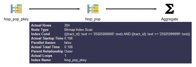
You can get more detailed information about each part by mousing over the node in the display.
Before wrapping up this section, we must pay homage to the tabular
explain plan created by Hubert Lubaczewski. Using his site, you can copy and paste the text output of your
EXPLAIN output, and it will show you
a beautifully formatted table, as shown in Figure 9-2.
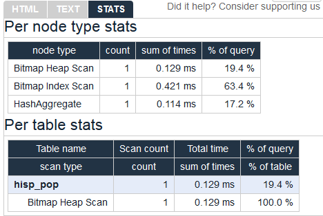
In the HTML tab, you’ll see a nicely reformatted color-coded table of the plan, with problem areas highlighted in vibrant colors, as shown in Figure 9-3. It has columns for exclusive time (time consumed by the parent step) and inclusive time (the time of the parent step plus its child steps).
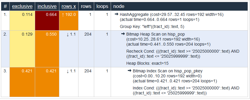
Although the HTML table in Figure 9-3 provides much the same information as our plain-text output, the color coding and the breakout of numbers makes it easier to digest. For example, yellow, brown, and red highlight potential bottlenecks.
The rows x column is the expected number of rows, while the rows column shows the actual number after execution. This reveals that, although our planner’s final step was expecting 192 records, we ended up with just one. Bad row estimates are often caused by out-of-date table statistics. It’s always a good habit to analyze tables frequently to update the statistics, especially right after an extensive update or insert.
The first step in optimizing performance is to determine which queries are bottlenecks. One monitoring extension useful for getting a handle on your most costly queries is pg_stat_statements. This extension provides metrics on running queries, the most frequently run queries, and how long each takes. Studying these metrics will help you determine where you need to focus your optimization efforts.
pg_stat_statements comes packaged with most PostgreSQL distributions but must be preloaded on startup to initiate its data-collection process:
In postgresql.conf, change
shared_preload_libraries = '' to
shared_preload_libraries = 'pg_stat_statements'.
In the customized options section of postgresql.conf, add the lines:
pg_stat_statements.max = 10000 pg_stat_statements.track = all
Restart your postgresql
service.
In any database you want to use for monitoring, enter
CREATE EXTENSION pg_stat_statements;.
The extension provides two key features:
A view called pg_stat_statements, which shows all the databases to which the currently
connected user has access.
A function called pg_stat_statements_reset, which
flushes the query log. This function can be run only by
superusers.
The query in Example 9-6 lists the
five most costly queries in the postgresql_book
database.
SELECT
query, calls, total_time, rows,
100.0*shared_blks_hit/NULLIF(shared_blks_hit+shared_blks_read,0) AS hit_percent
FROM pg_stat_statements As s INNER JOIN pg_database As d On d.oid = s.dbid
WHERE d.datname = 'postgresql_book'
ORDER BY total_time DESC LIMIT 5;The best and easiest way to improve query performance is to start with well-written queries. Four out of five queries we encounter are not written as efficiently as they could be.
There appear to be two primary causes for all this bad querying. First, we see people reuse SQL patterns without thinking. For example, if they successfully write a query using a left join, they will continue to use left join when incorporating more tables instead of considering the sometimes more appropriate inner join. Unlike other programming languages, the SQL language does not lend itself well to blind reuse.
Second, people don’t tend to keep up with the latest developments in their dialect of SQL. Don’t be oblivious to all the syntax-saving (and sanity-saving) addenda that have come along in new versions of PostgreSQL.
Writing efficient SQL takes practice. There’s no such thing as a wrong query as long as you get the expected result, but there is such a thing as a slow query. In this section, we point out some of the common mistakes we see people make. Although this book is about PostgreSQL, our recommendations are applicable to other relational databases as well.
A classic newbie mistake is to think of subqueries as independent entities. Unlike conventional programming languages, SQL doesn’t take kindly to black-boxing—writing a bunch of subqueries independently and then assembling them mindlessly to get the final result. You have to treat each query holistically. How you piece together data from different views and tables is every bit as important as how you go about retrieving the data in the first place.
The unnecessary use of subqueries, as shown in Example 9-7, is a common symptom of piecemeal thinking.
SELECT tract_id,
(SELECT COUNT(*) FROM census.facts As F
WHERE F.tract_id = T.tract_id) As num_facts,
(SELECT COUNT(*)
FROM census.lu_fact_types As Y
WHERE Y.fact_type_id IN (
SELECT fact_type_id
FROM census.facts F
WHERE F.tract_id = T.tract_id
)
) As num_fact_types
FROM census.lu_tracts As T;Example 9-7 can be more efficiently written as Example 9-8. This query, consolidating selects and using a join, is not only shorter than the prior one, but faster. If you have a larger dataset or weaker hardware, the difference could be even more pronounced.
SELECT T.tract_id,
COUNT(f.fact_type_id) As num_facts,
COUNT(DISTINCT fact_type_id) As num_fact_types
FROM census.lu_tracts As T LEFT JOIN census.facts As F ON T.tract_id = F.tract_id
GROUP BY T.tract_id;Figure 9-4 shows the graphical
plan for Example 9-7 (we’ll save you the
eyesore of seeing the gnarled output of the text EXPLAIN),
while Figure 9-5 shows the
tabular output from http://explain.depesz.com, revealing a great deal of
inefficiency.
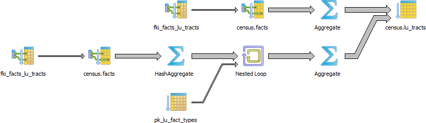
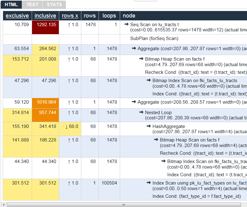
Figure 9-6 shows the graphical plan of Example 9-8, demonstrating how much less work goes on in it.
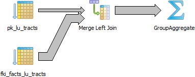
Keep in mind that we’re not asking you to avoid subqueries entirely. We’re only asking you to use them judiciously. When you do use them, pay extra attention to how you incorporate them into the main query. Finally, remember that a subquery should work with the main query, not independently of it.
SELECT * is wasteful. It’s akin to printing out a 1,000-page document when you
need only 10 pages. Besides the obvious downside of adding to network
traffic, there are two other drawbacks that you might not think
of.
First, PostgreSQL stores large blob and text objects using
TOAST (The Oversized-Attribute Storage Technique). TOAST
maintains side tables for PostgreSQL to store this extra data and may
chunk a single text field into multiple rows. So retrieving a large
field means that TOAST must assemble the data from several rows of a
side TOAST table. Imagine the extra processing if your table contains
text data the size of War and Peace and you perform
an unnecessary SELECT *.
Second, when you define views, you often will include more columns than you’ll need. You
might even go so far as to use SELECT * inside a view. This
is understandable and perfectly fine. PostgreSQL is smart enough to let
you request all the columns you want in your view definition and even
include complex calculations or joins without incurring penalty, as long
as no user runs a query referring to individual columns.
To drive home our point, let’s wrap our census in a view and use the slow subquery example from Example 9-7:
CREATE OR REPLACE VIEW vw_stats AS
SELECT tract_id,
(SELECT COUNT(*)
FROM census.facts As F
WHERE F.tract_id = T.tract_id) As num_facts,
(SELECT COUNT(*)
FROM census.lu_fact_types As Y
WHERE Y.fact_type_id IN (
SELECT fact_type_id
FROM census.facts F
WHERE F.tract_id = T.tract_id
)
) As num_fact_types
FROM census.lu_tracts As T;Now we query our view with this query:
SELECT tract_id FROM vw_stats;
Execution time is about 21 ms on our server because it doesn’t run
any computation for certain fields such as num_facts and
num_fact_types, fields we did not ask for. If you looked at
the plan, you may be startled to find that it never even touches the
facts table because it’s smart enough to know it doesn’t need to. But
suppose we enter:
SELECT * FROM vw_stats;
Our execution time skyrockets to 681 ms, and the plan is just as we had in Figure 9-4. Although our results in this example suffer the loss of just milliseconds, imagine tables with tens of millions of rows and hundreds of columns. Those milliseconds could translate into overtime at the office waiting for a query to finish.
We’re always surprised how frequently people forget about using the
ANSI SQL CASE expression. In many aggregate situations, a
CASE can obviate the need for inefficient subqueries. We’ll
demonstrate the point with two equivalent queries and their
corresponding plans. Example 9-9 uses
subqueries.
SELECT T.tract_id, COUNT(*) As tot, type_1.tot AS type_1
FROM
census.lu_tracts AS T LEFT JOIN
(SELECT tract_id, COUNT(*) As tot
FROM census.facts
WHERE fact_type_id = 131
GROUP BY tract_id
) As type_1 ON T.tract_id = type_1.tract_id LEFT JOIN
census.facts AS F ON T.tract_id = F.tract_id
GROUP BY T.tract_id, type_1.tot;Figure 9-7 shows the graphical plan of Example 9-9.
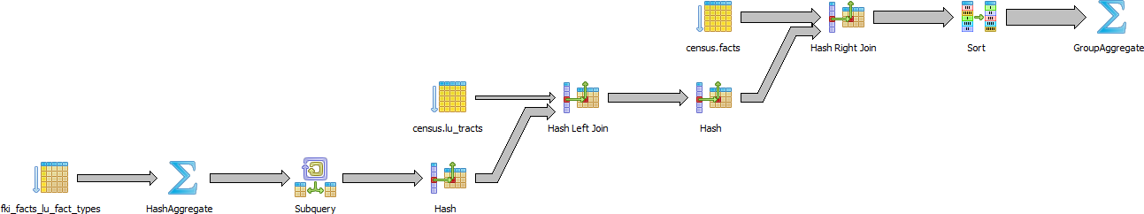
We now rewrite the query using CASE. You’ll find that
the economized query, shown in Example 9-10, is generally faster and
much easier to read.
SELECT T.tract_id, COUNT(*) As tot,
COUNT(CASE WHEN F.fact_type_id = 131 THEN 1 ELSE NULL END) AS type_1
FROM census.lu_tracts AS T LEFT JOIN census.facts AS F
ON T.tract_id = F.tract_id
GROUP BY T.tract_id;Figure 9-8 shows the graphical plan of Example 9-10.
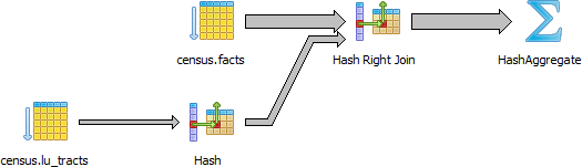
Even though our rewritten query still doesn’t use the
fact_type index, it’s faster than using subqueries because
the planner scans the facts table only once. A shorter plan
is generally not only easier to comprehend but also often performs
better than a longer one, although not always.
PostgreSQL 9.4 introduced the FILTER construct,
which we introduced in “FILTER Clause for Aggregates”. FILTER can often replace CASE in aggregate expressions. Not only is
this syntax more pleasant to look at, but in many situations it performs
better. We repeat Example 9-10
with the equivalent filter version in Example 9-11.
SELECT T.tract_id, COUNT(*) As tot,
COUNT(*) FILTER (WHERE F.fact_type_id = 131) AS type_1
FROM census.lu_tracts AS T LEFT JOIN census.facts AS F
ON T.tract_id = F.tract_id
GROUP BY T.tract_id;For this particular example, the FILTER performance is only about a millisecond
faster than our CASE version, and the
plans are more or less the same.
A parallelized query is one whose execution is distributed by the planner among multiple backend processes. By so doing, PostgreSQL is able to utilize multiple processor cores so that work completes in less time. Depending on the number of processor cores in your hardware, the time savings could be significant. Having two cores could halve your time; four could quarter your time, etc.
Parallelization was introduced in version 9.6. The kinds of queries available for parallelization are limited, usually consisting only of the most straightforward select statements. But with each new release, we expect the range of parallelizable queries to expand.
The kinds of queries that cannot be parallelized as of version 10.0 are:
Any data modifying queries, such as updates, inserts, and deletes.
Any data definition queries, such as the creation of new tables, columns, and indexes.
Queries called by cursors or for loops.
Some aggregates. Common ones like COUNT and SUM are parallelizable, but aggregates that include DISTINCT or ORDER BY are not.
Functions of your own creation. By default they are PARALLEL UNSAFE, but you can enable parallelization through the PARALLEL setting of the function as described in “Anatomy of PostgreSQL Functions”.
The following setting requirements are needed to enable the use of parallelism:
max_parallel_workers, a new setting in PostgreSQL 10, needs to be greater than zero
and less than or equal to max_worker_processes.
max_parallel_workers_per_gather needs
to be greater than zero and less than or equal to
max_worker_processes. For PostgreSQL 10, this
setting must also be less than or equal to
max_parallel_workers. You can apply this particular
setting at the session or function level.
How do you know if your query is a beneficiary of parallelization? Look in the plan. Parallelization is done by a part of the planner called a gather node. So if you see a gather node in your query plan, you have some kind of parallelization. A gather node contains exactly one plan, which it divides amongst what are called workers. Each worker runs as separate backend processes, each process working on a portion of the overall query. The results of workers are collected by a worker acting as the leader. The leader does the same work as other workers but has the added responsibility of collecting all the answers from fellow workers. If the gather node is the root node of a plan, the whole query will be run in parallel. If it’s lower down, only the subplan it encompasses will be parallelized.
For debugging purposes, you can invoke a setting called force_parallel_mode. When true,
it will encourage the planner to use parallel mode if a query is
parallelizable even when the planner concludes it’s not cost-effective
to do so. This setting is useful during debugging to figure out why a
query is not parallelized. Don’t switch on this setting in a production
environment, though!
The queries you’ve seen thus far in this chapter will not trigger a parallel plan because the cost of setting up the background workers outweighs the benefit. To confirm that our query takes longer when forced to be parallel, try the following:
set force_parallel_mode = true;
And then run Example 9-4 again. The output of the new plan is shown in Example 9-12.
Gather
(cost=1029.57..1051.65 rows=192 width=64)
(actual time=12.881..13.947 rows=1 loops=1)
Workers Planned: 1
Workers Launched: 1
Single Copy: true
-> HashAggregate
(cost=29.57..32.45 rows=192 width=64)
(actual time=0.230..0.231 rows=1 loops=1)
Group Key: "left"((tract_id)::text, 5)
-> Bitmap Heap Scan on hisp_pop
(cost=10.25..28.61 rows=192 width=36)
(actual time=0.127..0.184 rows=204 loops=1)
Recheck Cond:
(((tract_id)::text >= '25025000000'::text) AND
((tract_id)::text <= '25025999999'::text))
-> Bitmap Index Scan on hisp_pop_pkey
(cost=0.00..10.20 rows=192 width=0)
(actual time=0.106..0.106 rows=204 loops=1)
Index Cond:
(((tract_id)::text >= '25025000000'::text) AND
((tract_id)::text <= '25025999999'::text))
Planning time: 0.416 ms
Execution time: 16.160 msThe cost of organizing additional workers (even one) significantly increases the total time of the query.
Generally, parallelization is rarely worthwhile for queries that finish in a few milliseconds. But for queries over a ginormous dataset that normally take seconds or minutes to complete, parallelization is worth the initial setup cost.
To illustrate the benefit of parallelization, we downloaded a table from the US Bureau of Labor Statistics with 6.5 million rows of data and ran the query in Example 9-13.
set max_parallel_workers_per_gather=4; EXPLAIN ANALYZE VERBOSE SELECT COUNT(*), area_type_code FROM labor GROUP BY area_type_code ORDER BY area_type_code;
Finalize GroupAggregate
(cost=104596.49..104596.61 rows=3 width=10)
(actual time=500.440..500.444 rows=3 loops=1)
Output: COUNT(*), area_type_code
Group Key: labor.area_type_code
-> Sort
(cost=104596.49..104596.52 rows=12 width=10)
(actual time=500.433..500.435 rows=15 loops=1)
Output: area_type_code, (PARTIAL COUNT(*))
Sort Key: labor.area_type_code
Sort Method: quicksort Memory: 25kB
-> Gather
(cost=104595.05..104596.28 rows=12 width=10)
(actual time=500.159..500.382 rows=15 loops=1)
Output: area_type_code, (PARTIAL COUNT(*))
Workers Planned: 4
Workers Launched: 4
-> Partial HashAggregate
(cost=103595.05..103595.08 rows=3 width=10)
(actual time=483.081..483.082 rows=3 loops=5)
Output: area_type_code, PARTIAL count(*)
Group Key: labor.area_type_code
Worker 0: actual time=476.705..476.706 rows=3 loops=1
Worker 1: actual time=480.704..480.705 rows=3 loops=1
Worker 2: actual time=480.598..480.599 rows=3 loops=1
Worker 3: actual time=478.000..478.000 rows=3 loops=1
-> Parallel Seq Scan on public.labor
(cost=0.00..95516.70 rows=1615670 width=2)
(actual time=1.550..282.833 rows=1292543 loops=5)
Output: area_type_code
Worker 0: actual time=0.078..282.698 rows=1278313 loops=1
Worker 1: actual time=3.497..282.068 rows=1338095 loops=1
Worker 2: actual time=3.378..281.273 rows=1232359 loops=1
Worker 3: actual time=0.761..278.013 rows=1318569 loops=1
Planning time: 0.060 ms
Execution time: 512.667 msTo see the cost and timing without parallelization, set
max_parallel_workers_per_gather=0, and compare the plan, as
shown in Example 9-14.
set max_parallel_workers_per_gather=0; EXPLAIN ANALYZE VERBOSE SELECT COUNT(*), area_type_code FROM labor GROUP BY area_type_code ORDER BY area_type_code;
Sort
(cost=176300.24..176300.25 rows=3 width=10)
(actual time=1647.060..1647.060 rows=3 loops=1)
Output: (COUNT(*)), area_type_code
Sort Key: labor.area_type_code
Sort Method: quicksort Memory: 25kB
-> HashAggregate
(cost=176300.19..176300.22 rows=3 width=10)
(actual time=1647.025..1647.025 rows=3 loops=1)
Output: count(*), area_type_code
Group Key: labor.area_type_code
-> Seq Scan on public.labor
(cost=0.00..143986.79 rows=6462679 width=2)
(actual time=0.076..620.563 rows=6462713 loops=1)
Output: series_id, year, period, value, footnote_codes, area_type_code
Planning time: 0.054 ms
Execution time: 1647.115 msIn both cases, the output is the following:
count | area_type_code --------+--------------- 3718937 | M 2105205 | N 638571 | S (3 rows)
In the parallel plan, four workers each take about 280 ms to accomplish their portion of the task.
A parallel query has a particular scan strategy for partitioning the set of data among workers. In PostgreSQL 9.6, only a sequential scan is parallelizable. PostgreSQL 10 is also able to parallelize bitmap heap scans, index scans, and index-only scans. However, for index and index-only scans, only B-Tree indexes will parallelize. No such limitation exists for bitmap heap scans: for them, any index type will qualify. But in the bitmap heap scan, the building of the bitmap index is not parallelizable, so workers must wait for the bitmap index to be fully built.
Joins also benefit from parallelization. In PostgreSQL 9.6, nested loops and hash joins are parallelizable.
In nested loops, each worker matches its subset of data against a complete reference set of data shared by all workers.
In hash joins, each worker builds a separate copy of the hash table and joins this with their partitioned share of other tables. Thus, in a hash join, workers are doing redundant work by doing a full hash. So in cases where creating the hash table is expensive, a parallel hash join is less efficient than a nonparallel join.
In PostgreSQL 10, merge joins are parallelizable. Merge joins have a similar limitation to hash joins, in that one side of the join is repeated in its entirety by each worker.
The planner’s behavior is driven by the presence of indexes, cost settings, strategy settings, and its general perception of the distribution of data. In this section, we’ll go over various approaches for optimizing the planner’s behavior.
Although the PostgreSQL query planner doesn’t accept index hints as some other database products do, you can disable various strategy settings on a per-query or permanent basis to dissuade the planner from going down an unproductive path. All planner optimizing settings are documented in the section Planner Method Configuration of the manual. By default, all strategy settings are enabled, arming the planner with maximum flexibility. You can disable various strategies if you have some prior knowledge of the data. Keep in mind that disabling doesn’t necessarily mean that the planner will be barred from using the strategy. You’re only making a polite request to the planner to avoid it.
Two settings that we occasionally disable are enable_nestloop and
enable_seqscan. The reason is that these two
strategies tend to be the slowest, though not in all cases. Although you
can disable them, the planner can still use them when it has no viable
alternative. When you do see them being used, it’s a good idea to
double-check that the planner is using them out of efficiency, and not
out of ignorance. One quick way to check is to disable them. If they are
used by default but not used when you disable them, compare the actual
costs between the two cases to confirm that using them is more efficient
than not using them.
When the planner decides to perform a sequential scan, it loops through all the
rows of a table. It opts for this route when it finds no index that
could satisfy a query condition, or it concludes that using an index is
more costly than scanning the table. If you disable the sequential scan
strategy, and the planner still insists on using it, this means that
indexes are missing or that the planner can’t use the indexes you have
in place for the particular query. Two common mistakes people make are
to leave useful indexes out of their tables or to put in indexes that
can’t be used by their queries. An easy way to check whether your
indexes are being used is to query the pg_stat_user_indexes and pg_stat_user_tables views. To target slow
queries, use the pg_stat_statements extension described in
“Gathering Statistics on Statements”.
Let’s start off with a query against the table we created in Example 7-22. We’ll add a GIN index on the array column. GIN indexes are among the few indexes you can use to index arrays:
CREATE INDEX idx_lu_fact_types ON census.lu_fact_types USING gin (fact_subcats);
To test our index, we’ll execute a query to find all rows with
subcats containing “White alone” or “Asian alone.” We explicitly enabled
sequential scan even though it’s the default setting, just to be sure.
The accompanying EXPLAIN output is shown in Example 9-15.
setenable_seqscan=true;EXPLAIN(ANALYZE)SELECT*FROMcensus.lu_fact_typesWHEREfact_subcats&&'{White alone, Black alone}'::varchar[];
SeqScanonlu_fact_types(cost=0.00..2.85rows=2width=200)actualtime=0.066..0.076rows=2loops=1)Filter:(fact_subcats&&'{"White alone","Black alone"}'::charactervarying[])RowsRemovedbyFilter:66Planningtime:0.182msExecutiontime:0.108ms
Observe that when enable_seqscan is enabled,
our index is not being used and the planner has chosen to do a
sequential scan. This could be because our table is so small or because
the index we have is no good for this query. If we repeat the query but
turn off sequential scan beforehand, as shown in Example 9-16, we can see
that we have succeeded in forcing the planner to use the index.
setenable_seqscan=false;EXPLAIN(ANALYZE)SELECT*FROMcensus.lu_fact_typesWHEREfact_subcats&&'{White alone, Black alone}'::varchar[];
BitmapHeapScanonlu_fact_types(cost=12.02..14.04rows=2width=200)(actualtime=0.058..0.058rows=2loops=1)RecheckCond:(fact_subcats&&'{"White alone","Black alone"}'::charactervarying[])HeapBlocks:exact=1->BitmapIndexScanonidx_lu_fact_types(cost=0.00..12.02rows=2width=0)(actualtime=0.048..0.048rows=2loops=1)IndexCond:(fact_subcats&&'{"White alone","Black alone"}'::charactervarying[])Planningtime:0.230msExecutiontime:0.119ms
From this plan, we learn that our index can be used but ends up making the query take longer because the cost is more than doing a sequential scan. Therefore, under normal circumstances, the planner will opt for the sequential scan. As we add more data to our table, we’ll probably find that the planner changes strategies to an index scan.
In contrast to the previous example, suppose we were to write a query of the form:
SELECT * FROM census.lu_fact_types WHERE 'White alone' = ANY(fact_subcats);
We would discover that, regardless of how we set
enable_seqscan, the planner will always perform a
sequential scan because the index we have in place can’t service this
query. So it is important to consider which indexes will be useful and
to write queries to take advantage of them. And experiment, experiment,
experiment!
Despite what you might think or hope, the query planner is not a magician. Its decisions follow prescribed logic that’s far beyond the scope of this book. The rules that the planner follows depend heavily on the current state of the data. The planner can’t possibly scan all the tables and rows prior to formulating its plan. That would be self-defeating. Instead, it relies on aggregated statistics about the data.
Therefore, having accurate and current stats is crucial for the
planner to make the right decision. If stats differ greatly from
reality, the planner will often come up with bad plans, the most
detrimental of these being unnecessary sequential table scans.
Generally, only about 20 percent of the entire table is sampled to
produce stats. This percentage could be even lower for very large
tables. You can control the number of rows sampled on a column-by-column
basis by setting the STATISTICS value.
To get a sense of the information culled and used by the planner,
query the pg_stats table, as illustrated in Example 9-17.
SELECTattnameAscolname,n_distinct,most_common_valsAScommon_vals,most_common_freqsAsdist_freqFROMpg_statsWHEREtablename='facts'ORDERBYschemaname,tablename,attname;
colname|n_distinct|common_vals|dist_freq-------------+------------+------------------+------------------------------fact_type_id|68|{135,113...|{0.0157,0.0156333,...perc|985|{0.00,...|{0.1845,0.0579333,0.056...tract_id|1478|{25025090300...|{0.00116667,0.00106667,0.0...val|3391|{0.000,1.000,2...|{0.2116,0.0681333,0...yr|2|{2011,2010}|{0.748933,0.251067}
pg_stats gives the planner a sense of how actual
values are dispersed within a given column and lets it plan accordingly.
The pg_stats table is constantly updated as a background
process. After a large data load or a major deletion, you should
manually update the stats by executing VACUUM ANALYZE. VACUUM
permanently removes deleted rows from tables; ANALYZE
updates the stats.
For columns that participate often in joins and are used heavily
in WHERE clauses, consider increasing the number of sampled
rows:
ALTER TABLE census.facts ALTER COLUMN fact_type_id SET STATISTICS 1000;
Version 10 introduced support for multicolumn stats via
the new CREATE
STATISTICS DDL construct. This feature allows you to create
stats against a combination of columns. A multicolumn stat is useful if
you have columns that are correlated in value. Say, for example, that
you have a particular kind of data for only one year and not other
years. In that case, you might want to create a compound stat for
fact_type_id and yr as shown in Example 9-18.
CREATESTATISTICScensus.stats_facts_type_yr_dep_dist(dependencies,ndistinct)ONfact_type_id,yrFROMcensus.facts;ANALYZEcensus.facts;
A CREATE STATISTICS statement must specify two or more columns in
a single table. Example 9-18 creates
stats on the columns fact_type_id and
yr in the census.facts table. The statistics should also
be named, although that is optional. If you specify a schema as part of
the name, the statistics will be created in that schema; otherwise, they
get created in the default schema.
You can collect two kinds of statistics, and must specify one or both in your statement:
The dependencies statistic
catalogs dependencies between columns. For example,
zip code 02109 is seen only with Boston in the city
column. dependencies statistics are used only to
optimize queries with equalities, such as a query specifying
city = 'Boston' and zip = '02109'.
The ndistinct statistic
catalogs how often column values are seen together and
tries to catalog statistics for each group of columns.
ndistinct statistics are only used for improving
GROUP BY clauses. Specifically, they are useful only
on queries that group by all the columns in your statistic.
Statistics created using CREATE STATISTICS are stored in the table
pg_statistic_ext and can be dropped
using DROP STATISTICS. Similar to other statistics, they are computed during an ANALYZE
run, which happens during the system vacuum analyze process. After
creating a table, it’s a good idea to run an ANALYZE on it so the new
stats can be used immediately.
Another setting that influences the planner is the random_page_cost
(RPC) ratio, which is the relative cost of disk access when retrieving a
record using a sequential read versus random access. Generally, the
faster (and more expensive) the physical disk, the lower the ratio. The
default value for RPC is 4, which works well for most mechanical hard
drives on the market today. The use of solid-state drives (SSDs),
high-end storage area networks (SANs), or cloud storage makes it worth
tweaking this value.
You can set the RPC ratio per database, per server, or per
tablespace. At the server level, it makes most sense to set the ratio in
the postgresql.conf file. If you
have different kinds of disks, you can set the values at the
tablespace level using the ALTER TABLESPACE command:
ALTER TABLESPACEpg_defaultSET (random_page_cost=2);
Details about this setting can be found at Random Page Cost Revisited. The article suggests the following settings:
If you execute a complex query that takes a while to run, subsequent runs are often much faster. Thank caching. If the same query executes in sequence, by the same user or different users, and no changes have been made to the underlying data, you should get back the same result. As long as there’s space in memory to cache the data, the planner can skip replanning or reretrieving. Using common table expressions and immutable functions in your queries encourages caching.
How do you check what’s in the current cache? You can install the pg_buffercache extension:
CREATE EXTENSION pg_buffercache;
You can then run a query against the pg_buffercache view, as shown in Example 9-19.
SELECT
C.relname,
COUNT(CASE WHEN B.isdirty THEN 1 ELSE NULL END) As dirty_buffers,
COUNT(*) As num_buffers
FROM
pg_class AS C INNER JOIN
pg_buffercache B ON C.relfilenode = B.relfilenode INNER JOIN
pg_database D ON B.reldatabase = D.oid AND D.datname = current_database()
WHERE C.relname IN ('facts','lu_fact_types')
GROUP BY C.relname;Example 9-19 returns the number of
buffered pages of the facts and lu_fact_types
tables. Of course, to actually see buffered rows, you need to run a query.
Try this one:
SELECT T.fact_subcats[2], COUNT(*) As num_fact FROM census.facts As F INNER JOIN census.lu_fact_types AS T ON F.fact_type_id = T.fact_type_id GROUP BY T.fact_subcats[2];
The second time you run the query, you should notice at least a 10% performance speed increase and should see the following cached in the buffer:
relname | dirty_buffers | num_buffers --------------+---------------+------------ facts | 0 | 736 lu_fact_types | 0 | 4
The more onboard memory you have dedicated to the cache, the more
room you’ll have to cache data. You can set the amount of dedicated memory
by changing the shared_buffers setting in postgresql.conf. Don’t go overboard; raising
shared_buffers too much will bloat your cache, leading
to more time wasted scanning the cache.
Nowadays, there’s no shortage of onboard memory. You can take advantage of this by precaching commonly used tables using an extension called pg_prewarm. pg_prewarm lets you prime your PostgreSQL by loading data from commonly used tables into memory so that the first user to hit the database can experience the same performance boost offered by caching as later users. A good article that describes this feature is Prewarming Relational Data.
PostgreSQL has a number of options for sharing data with external
servers or data sources. The first option is the built-in replication options of PostgreSQL, which allow you to create a
copy of your server ready to run on another PostgreSQL server. The second
option is to use third-party add-ons, many of which are freely available and
time-tested. The third option is to use a foreign data wrapper (FDW). FDWs
give you the flexibility to query from a wide array of external data
sources. Since version 9.3, some FDWs also permit updating: these include postgres_fdw, hadoop_fdw, and ogr_fdw
(see “Querying Other Tabular Formats with ogr_fdw”).
The reasons for replicating your databases distill down to two: availability and scalability. Availability is assured by providing a redundant server so that, if your main server goes down, you have another that can immediately assume its role. For small databases, you could just make sure you have another physical server ready and restore the database onto it. But for large databases (in the terabytes), the restore itself could take hours, if not days. To avoid downtime, you’ll need to replicate.
The other motivation for replications is scalability. Suppose you set up a database to breed fancy elephant shrews for profit. After a few years of breeding, you now have thousands of elephant shrews. People all over the world come to your site to gawk and purchase. You’re overwhelmed by the traffic, but replication comes to your aid. You arrange a read-only slave server to replicate with your main server. Then you direct the countless gawkers to the slave, and let only serious buyers onto the master server to finalize their purchases.
Before we get too carried away, we should introduce some common lingo in PostgreSQL replication:
The master server is the database server sourcing the data being replicated and where all updates take place. You’re allowed only one master when using the built-in server replication features of PostgreSQL. Plans are in place to support multimaster replication scenarios. Watch for it in future releases. You may also hear the term publisher used to mean the provider of the data. Publisher/subscriber terminology gains more traction in PostgreSQL 10 for built-in logical replication.
A slave server consumes the replicated data and provides a replica of the master. More aesthetically pleasing terms such as subscriber and agent have been bandied about, but slave is still the most apropos. PostgreSQL built-in replication supports only read-only slaves at this time.
WAL is the log that keeps track of all transactions, often referred to as the transaction log in other database products. To stage replication, PostgreSQL simply makes the logs available to the slaves. Once slaves have pulled the logs, they just need to execute the transactions therein.
A transaction on the master will not be considered complete until at
least one synchronous slave listed in
synchronous_standby_names updates and reports
back. Prior to version 9.6, if any synchronous slave responds, the
transaction is complete. In version 9.6 and higher, the number of
standbys that must respond is configurable using the
synchronous_standby_names postgresql.conf
configuration variable. Version 10 introduced the keywords FIRST
and ANY that can be added to the synchronous_standby_names
configuration variable that dictates which nodes need to report
back. FIRST is the default behavior if not specified and the
behavior of 9.6.
A transaction on the master will commit even if no slave updates. This is expedient for distant servers where you don’t want transactions to wait because of network latency, but the downside is that your dataset on the slave might lag behind. Should the lag be severe, the slave might need to be reinitialized if the transaction it needs to continue has already been removed from the WAL logs.
To minimize the risk of WALs being removed before all slaves have used them, version 9.4 introduced replication slots. A replication slot is a contract between a slave and its master whereby the master will not wipe out any WAL logs that are still needed by any replication slots. The hazard is that if a slave holding a replication slot fails or loses communication for a long time, the master will keep the WALS indefinitely and run out of disk space and shut down.
The slave does not require direct file access between master and slaves. Instead, it relies on the PostgreSQL connection protocol to transmit the WALs.
Slaves can receive logs from nearby slaves instead of directly from the master. This allows a slave to behave like a master for replication purposes. The slave remains read-only. When a slave acts both as a receiver and a sender, it is called a cascading standby.
This is a new replication option in version 10 that allows the
replication of individual tables instead of requiring the whole
server cluster to be replicated. It relies on a feature called logical decoding, which
extracts changes to a database table from the WAL logs in an
easy-to-understand format without detailed knowledge of the
database’s internal state. Logical decoding has existed since 9.4
and has been used by some extensions for auditing and providing
replication. This new feature comes with the new DDL commands CREATE PUBLICATION and
CREATE SUBSCRIPTION for designating what tables to
replicate and what servers and corresponding database to send data
to.
To use this feature, you must set wal_level to
logical.
Refer to Logical Replication in PostgreSQL 10 for an example of its use.
Remastering promotes a slave to be the master. Version 9.3 introduced streaming-only remastering, which eliminates the need for remastering to consult a WAL archive; it can be done via streaming, and slaves no longer need to be recloned. As of version 9.4, though, a restart is still required. This may change in future releases.
PostgreSQL binary replication replicates only changes that are
transactional. Because any DDL command is transactional, the creation of tables,
views, and installation of extensions can be replicated as well. But
because unlogged table inserts and updates are not transactional, they
cannot be replicated. When installing extensions, you should make sure
all slaves have the binaries for the extension and version of extension
you are installing; otherwise, replication will fail when the CREATE EXTENSION command is executed on
the master.
PostgreSQL’s stock replication relies on WAL shipping. Streaming replication slaves should be running the same OS and bitness (32-bit/64-bit) as the master. It is also recommended that all servers be running the same minor version as the master, though running the same patch level (microversion) is not required. Though not recommended, the slave and master can be running a different minor version. In this case, it’s preferable for the slave to be running a newer minor version than the master.
Support for built-in replication improved over the following PostgreSQL releases:
Version 9.4 added replication slots. A replication slot is a contract between a master and a slave that requires the master to hold on to WALs until a slave is done processing them.
Version 9.5 added several functions for monitoring the progress of replication: refer to Replication Progress Tracking in the documentation.
Version 9.6 introduced multiple standby servers in synchronous replication for increased reliability.
Version 10 introduced built-in logical replication, which allows the replication of individual tables. The other benefit of logical replication is that a slave can have databases and tables of its own that are not part of replication and that can be updated on the slave. Version 10 also introduced temporary replication slots, which allow a process to create a replication slot on a one-time basis and have it disappear after the session is over. This is particularly useful for initializing a new copy of the server via pg_basebackup.
Although logical replication is built into PostgreSQL for the first time in version 10, you can use logical replication in PostgreSQL 9.4 and higher versions of PostgreSQL 9 through the open source PostgreSQL extension pglogical. If you need to replicate between version 10 and versions 9.4−9.6, you’ll need to have pglogical installed on both version 10 and the lower-versioned server. For logical replication between version 10 and future versions of PostgreSQL, you can use the built-in logical replication feature.
As alternatives to PostgreSQL’s built-in replication, common third-party options abound. Slony and Bucardo are two popular open source ones. Although PostgreSQL is improving replication with each new release, Slony, Bucardo, and other third-party replication options still offer more flexibility. Slony and Bucardo allow you to replicate individual databases or even tables instead of the entire server. They also don’t require that all masters and slaves run the same PostgreSQL version and OS. Both also support multimaster scenarios. However, both rely on additional triggers and possible addition of columns to tables to initiate the replication and often don’t replicate DDL commands for rare actions such as creating new tables, installing extensions, and so on. Thus, they require more manual intervention, such as the addition of triggers, additional table fields, or views.
We urge you to consult a comparison matrix of popular third-party options before deciding what to use.
Let’s go over the steps to replicate the whole server cluster. We’ll take advantage of streaming replication. Recall that streaming replication only requires connections at the PostgreSQL database level between the master and slaves.
The steps for setting up the master are:
CREATE ROLE pgrepuser REPLICATION LOGIN PASSWORD 'woohoo';
Alter the following configuration settings in postgresql.auto.conf. These can be done
using ALTER SYSTEM set variable=value followed by
SELECT pg_reload_conf(); without the need to touch the
physical config file:
listen_addresses = * wal_level = hot_standby archive_mode = on max_wal_senders = 5 wal_keep_segments = 10
If you want to use logical replication to do partial replication of only some tables, you’ll need to set wal_level = logical. Logical does more logging than hot_standby so will also work for doing full server replication.
These settings are described in Server Configuration:
Replication. You may want to set wal_keep_segments higher if
your servers are far apart and your production server has a lot of
transactions. If you are running version 9.6 or above, you should
use replica instead of hot_standby for the
wal_level. hot_standby is still
accepted in 9.6 for backward compatibility, but will be read as
replica.
Add the archive_command
configuration directive to postgresql.auto.conf or use ALTER
SYSTEM to indicate where the WALs will be saved. With
streaming, you’re free to choose any directory. More details on this
setting can be found in the PostgreSQL PGStandby
documentation.
On Linux/Unix, your archive_command line should look
something like:
archive_command = 'cp %p ../archive/%f'
You can also use rsync instead of cp
if you want to store the WALs on a different server:
archive_command = 'rsync -av %p postgres@192.168.0.10:archive/%f'
archive_command = 'copy %p ..\\archive\\%f'
Add a rule to pg_hba.conf
allowing the slaves to replicate. As an example, the following
rule will allow a PostgreSQL account named pgrepuser on a server on your private network with an IP address
in the range 192.168.0.1 to 192.168.0.254 to replicate using an md5
password:
host replication pgrepuser 192.168.0.0/24 md5
Restart the PostgreSQL service for the settings to take effect.
Use the pg_basebackup utility, found in the bin
folder of your PostgreSQL installation, to create a cluster backup.
This will create a copy of the data cluster files in the specified
directory.
When using pg_basebackup, use the
--xlog-method-stream switch to also copy over the WAL
logs and the -R switch to automatically create a config
file. The command --xlog-method-stream will spawn
another database connection for copying the WALs.
In version 10 and above, the pg_xlog directory is pg_wal.
In the following example, we are on the slave server and performing a streaming basebackup from our master server (192.168.0.1):
pg_basebackup -D /target_dir -h 192.168.0.1 \ --port=5432 --checkpoint=fast --xlog-method=stream -R
If you are using pg_basebackup primarily for backup purposes, you
can use the tarred/compressed form, which will create a tar.gz file in the target_dir folder for each table space.
-X is shorthand for --xlog-method. The tarred/compression format
does not support streaming logs, so you have to resort to fetching the
logs with that format:
pg_basebackup -Z9 -D /target_dir/ -h 192.168.0.1 -Ft -Xfetch
For backup, you will want to augment your backup to include transaction log shipping backup using pg_receivexlog for versions prior to 10. For versions 10 and above, pg_receivexlog was renamed to pg_receivewal. This you’ll want to keep running as a cronjob or service to continually make log backups.
This part is not needed for logical replication. To minimize headaches, slaves should have the same configuration as the master, especially if you’ll be using them for failover. They must also have the same set of PostgreSQL extensions installed in binary; otherwise, when CREATE EXTENSION is played back, it will fail and stop restore. In order for the server to be a slave, it must be able to play back the WAL transactions of the master. The steps for creating a slave are as follows:
Create a new instance of PostgreSQL with the same version (preferably even microversions) as your master server. For PostgreSQL, keeping servers identical for microversions is not a requirement, and you’re welcome to experiment and see how far you can deviate.
Shut down PostgreSQL on the new slave.
Overwrite the data folder files with those you generated with pg_basebackup.
Add the following configuration setting to the postgresql.auto.conf file:
hot_standby = on max_connections = 20 #set to higher or equal to master
You don’t need to run the slaves on the same port as the
master, so you can optionally change the port either via postgresql.auto.conf, postgresql.conf, or via some other
OS-specific startup script that sets the PGPORT
environment variable before startup.
Create a new file in the data folder called recovery.conf with the following contents, but substitute the actual hostname, IP address, and port of your master on the second line. This file is automatically created if you used pg_basebackup. You will have to add the trigger_file line though.
The application_name is optional but useful if you want to track the replica in postgresql system views:
standby_mode = 'on' primary_conninfo = 'host=192.168.0.1 port=5432 user=pgrepuser