Table of Contents
System-Level Controls and Settings
Introduction to the Instruction Set
Functions and Function Invocation
Branching and Conditional Execution
Asynchronous and Ad-Hoc Execution
Chapter 4: Debugging and Automation
The Debugging Tools and Basic Commands
Scripting with the Debugging Tools
Useful Extensions, Tools, and Resources
A Survey of Obfuscation Techniques
A Survey of Deobfuscation Techniques
The x86 is little-endian architecture based on the Intel 8086 processor. For the purpose of our chapter, x86 is the 32-bit implementation of the Intel architecture (IA-32) as defined in the Intel Software Development Manual. Generally speaking, it can operate in two modes: real and protected. Real mode is the processor state when it is first powered on and only supports a 16-bit instruction set. Protected mode is the processor state supporting virtual memory, paging, and other features; it is the state in which modern operating systems execute. The 64-bit extension of the architecture is called x64 or x86-64. This chapter discusses the x86 architecture operating in protected mode.
x86 supports the concept of privilege separation through an abstraction called ring level. The processor supports four ring levels, numbered from 0 to 3. (Rings 1 and 2 are not commonly used so they are not discussed here.) Ring 0 is the highest privilege level and can modify all system settings. Ring 3 is the lowest privileged level and can only read/modify a subset of system settings. Hence, modern operating systems typically implement user/kernel privilege separation by having user-mode applications run in ring 3, and the kernel in ring 0. The ring level is encoded in the CS register and sometimes referred to as the current privilege level (CPL) in official documentation.
This chapter discusses the x86/IA-32 architecture as defined in the Intel 64 and IA-32 Architectures Software Developer's Manual, Volumes 1–3 (www.intel.com/content/www/us/en/processors/architectures-software-developer-manuals.html).
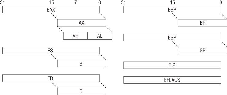
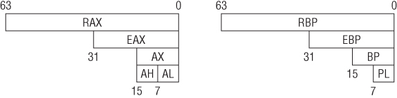
When operating in protected mode, the x86 architecture has eight 32-bit general-purpose registers (GPRs): EAX, EBX, ECX, EDX, EDI, ESI, EBP, and ESP. Some of them can be further divided into 8- and 16-bit registers. The instruction pointer is stored in the EIP register. The register set is illustrated in Figure 1.1. Table 1.1 describes some of these GPRs and how they are used.
Table 1.1 Some GPRs and Their Usage
| Register | Purpose |
| ECX | Counter in loops |
| ESI | Source in string/memory operations |
| EDI | Destination in string/memory operations |
| EBP | Base frame pointer |
| ESP | Stack pointer |
The common data types are as follows:
The 32-bit EFLAGS register is used to store the status of arithmetic operations and other execution states (e.g., trap flag). For example, if the previous “add” operation resulted in a zero, the ZF flag will be set to 1. The flags in EFLAGS are primarily used to implement conditional branching.
In addition to the GPRs, EIP, and EFLAGS, there are also registers that control important low-level system mechanisms such as virtual memory, interrupts, and debugging. For example, CR0 controls whether paging is on or off, CR2 contains the linear address that caused a page fault, CR3 is the base address of a paging data structure, and CR4 controls the hardware virtualization settings. DR0–DR7 are used to set memory breakpoints. We will come back to these registers later in the “System Mechanism” section.
There are also model-specific registers (MSRs). As the name implies, these registers may vary between different processors by Intel and AMD. Each MSR is identified by name and a 32-bit number, and read/written to through the RDMSR/WRMSR instructions. They are accessible only to code running in ring 0 and typically used to store special counters and implement low-level functionality. For example, the SYSENTER instruction transfers execution to the address stored in the IA32_SYSENTER_EIP MSR (0x176), which is usually the operating system's system call handler. MSRs are discussed throughout the book as they come up.
The x86 instruction set allows a high level of flexibility in terms of data movement between registers and memory. The movement can be classified into five general methods:
The first four methods are supported by all modern architectures, but the last one is specific to x86. A classical RISC architecture like ARM can only read/write data from/to memory with load/store instructions (LDR and STR, respectively); for example, a simple operation like incrementing a value in memory requires three instructions:
On x86, such an operation would require only one instruction (either INC or ADD) because it can directly access memory. The MOVS instruction can read and write memory at the same time.
ARM
01: 1B 68         LDR      R3, [R3]
; read the value at address R3
02: 5A 1C         ADDS     R2, R3, #1
; add 1 to it
03: 1A 60         STR      R2, [R3]
; write updated value back to address R3
x86
01: FF 00         inc      dword ptr [eax]
; directly increment value at address EAX
Another important characteristic is that x86 uses variable-length instruction size: the instruction length can range from 1 to 15 bytes. On ARM, instructions are either 2 or 4 bytes in length.
Depending on the assembler/disassembler, there are two syntax notations for x86 assembly code, Intel and AT&T:
Intel
mov ecx, AABBCCDDh
mov ecx, [eax]
mov ecx, eax
AT&T
movl $0xAABBCCDD, %ecx
movl (%eax), %ecx
movl %eax, %ecx
It is important to note that these are the same instructions but written differently. There are several differences between Intel and AT&T notation, but the most notable ones are as follows:
Disassemblers/assemblers and other reverse-engineering tools (IDA Pro, OllyDbg, MASM, etc.) on Windows typically use Intel notation, whereas those on UNIX frequently follow AT&T notation (GCC). In practice, Intel notation is the dominant form and is used throughout this book.
Instructions operate on values that come from registers or main memory. The most common instruction for moving data is MOV. The simplest usage is to move a register or immediate to register. For example:
01: BE 3F 00 0F 00   mov   esi, 0F003Fh ; set ESI = 0xF003
02: 8B F1            mov   esi, ecx     ; set ESI = ECX
The next common usage is to move data to/from memory. Similar to other assembly language conventions, x86 uses square brackets ([]) to indicate memory access. (The only exception to this is the LEA instruction, which uses [] but does not actually reference memory.) Memory access can be specified in several different ways, so we will begin with the simplest case:
Assembly
01: C7 00 01 00 00+  mov   dword ptr [eax], 1
; set the memory at address EAX to 1
02: 8B 08            mov   ecx, [eax]
; set ECX to the value at address EAX
03: 89 18            mov   [eax], ebx
; set the memory at address EAX to EBX
04: 89 46 34         mov   [esi+34h], eax
; set the memory address at (ESI+34) to EAX
05: 8B 46 34         mov   eax, [esi+34h]
; set EAX to the value at address (EAX+34)
06: 8B 14 01         mov   edx, [ecx+eax]
; set EDX to the value at address (ECX+EAX)
Pseudo C
01: *eax = 1;
02: ecx = *eax;
03: *eax = ebx;
04: *(esi+34) = eax;
05: eax = *(esi+34);
06: edx = *(ecx+eax);
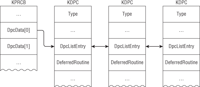
These examples demonstrate memory access through a base register and offset, where offset can be a register or immediate. This form is commonly used to access structure members or data buffers at a location computed at runtime. For example, suppose that ECX points to a structure of type KDPC with the layout
kd> dt nt!_KDPC
   +0x000 Type             : UChar
   +0x001 Importance       : UChar
   +0x002 Number           : Uint2B
   +0x004 DpcListEntry     : _LIST_ENTRY
   +0x00c DeferredRoutine  : Ptr32     void
   +0x010 DeferredContext  : Ptr32 Void
   +0x014 SystemArgument1  : Ptr32 Void
   +0x018 SystemArgument2  : Ptr32 Void
   +0x01c DpcData          : Ptr32 Void
and used in the following context:
Assembly
01: 8B 45 0C         mov   eax, [ebp+0Ch]
02: 83 61 1C 00      and   dword ptr [ecx+1Ch], 0
03: 89 41 0C         mov   [ecx+0Ch], eax
04: 8B 45 10         mov   eax, [ebp+10h]
05: C7 01 13 01 00+  mov   dword ptr [ecx], 113h
06: 89 41 10         mov   [ecx+10h], eax
Pseudo C
KDPC *p = …;
p->DpcData = NULL;
p->DeferredRoutine = …;
*(int *)p = 0x113;
p->DeferredContext = …;
Line 1 reads a value from memory and stores it in EAX. The DeferredRoutine field is set to this value in line 3. Line 2 clears the DpcData field by AND'ing it with 0. Line 4 reads another value from memory and stores it in EAX. The DeferredContext field is set to this value in line 6.
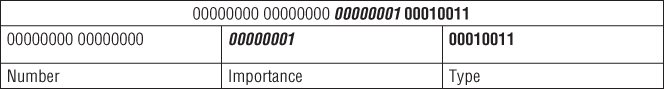
Line 5 writes the double-word value 0x113 to the base of the structure. Why does it write a double-word value at the base if the first field is only 1 byte in size? Wouldn't that implicitly set the Importance and Number fields as well? The answer is yes. Figure 1.2 shows the result of converting 0x113 to binary.
The Type field is set to 0x13 (bold bits), Importance is set to 0x1 (underlined bits), and Number is set to 0x0 (the remaining bits). By writing one value, the code managed to initialize three fields with a single instruction! The code could have been written as follows:
01: 8B 45 0C         mov   eax, [ebp+0Ch]
02: 83 61 1C 00      and   dword ptr [ecx+1Ch], 0
03: 89 41 0C         mov   [ecx+0Ch], eax
04: 8B 45 10         mov   eax, [ebp+10h]
05: C6 01 13         mov   byte ptr [ecx],13h
06: C6 41 01 01      mov   byte ptr [ecx+1],1
07: 66 C7 41 02 00+  mov   word ptr [ecx+2],0
08: 89 41 10         mov   [ecx+10h], eax
The compiler decided to fold three instructions into one because it knew the constants ahead of time and wants to save space. The three-instruction version occupies 13 bytes (the extra byte in line 7 is not shown), whereas the one-instruction version occupies 6 bytes. Another interesting observation is that memory access can be done at three granularity levels: byte (line 5–6), word (line 6), and double-word (line 1–4, 8). The default granularity is 4 bytes, which can be changed to 1 or 2 bytes with an override prefix. In the example, the override prefix bytes are C6 and 66 (italicized). Other prefixes are discussed as they come up.
The next memory access form is commonly used to access array-type objects. Generally, the format is as follows: [Base + Index * scale]. This is best understood through examples:
01: 8B 34 B5 40 05+  mov   esi, _KdLogBuffer[esi*4]
; always written as  mov   esi, [_KdLogBuffer + esi * 4]
; _KdLogBuffer is the base address of a global array and
; ESI is the index; we know that each element in the array
; is 4 bytes in length (hence the scaling factor)
02: 89 04 F7         mov   [edi+esi*8], eax
; here is EDI is the array base address; ESI is the array
; index; element size is 8.
In practice, this is observed in code looping over an array. For example:
01:                loop_start:
02: 8B 47 04         mov   eax, [edi+4]
03: 8B 04 98         mov   eax, [eax+ebx*4]
04: 85 C0            test  eax, eax
…
05: 74 14            jz    short loc_7F627F
06:                loc_7F627F:
07: 43               inc   ebx
08: 3B 1F            cmp   ebx, [edi]
09: 7C DD            jl    short loop_start
Line 2 reads a double-word from offset +4 from EDI and then uses it as the base address into an array in line 3; hence, you know that EDI is likely a structure that has an array at +4. Line 7 increments the index. Line 8 compares the index against a value at offset +0 in the same structure. Given this info, this small loop can be decompiled as follows:
typedef struct _FOO
{
    DWORD size;        // +0x00
    DWORD array[…];  // +0x04
} FOO, *PFOO;
PFOO bar = …;
for (i = …; i < bar->size; i++) {
    if (bar->array[i] != 0) {
    …
    }
}
The MOVSB/MOVSW/MOVSD instructions move data with 1-, 2-, or 4-byte granularity between two memory addresses. They implicitly use EDI/ESI as the destination/source address, respectively. In addition, they also automatically update the source/destination address depending on the direction flag (DF) flag in EFLAGS. If DF is 0, the addresses are decremented; otherwise, they are incremented. These instructions are typically used to implement string or memory copy functions when the length is known at compile time. In some cases, they are accompanied by the REP prefix, which repeats an instruction up to ECX times. Consider the following example:
Assembly
01: BE 28 B5 41 00   mov   esi, offset _RamdiskBootDiskGuid
; ESI = pointer to RamdiskBootDiskGuid
02: 8D BD 40 FF FF+  lea   edi, [ebp-0C0h]
; EDI is an address somewhere on the stack
03: A5               movsd
; copies 4 bytes from EDI to ESI; increment each by 4
04: A5               movsd
; same as above
05: A5               movsd
; save as above
06: A5               movsd
; same as above
Pseudo C
/* a GUID is 16-byte structure */
GUID RamDiskBootDiskGuid = …; // global
…
GUID foo;
memcpy(&foo, &RamdiskBootDiskGuid, sizeof(GUID));
Line 2 deserves some special attention. Although the LEA instruction uses [], it actually does not read from a memory address; it simply evaluates the expression in square brackets and puts the result in the destination register. For example, if EBP were 0x1000, then EDI would be 0xF40 (=0x1000 – 0xC0) after executing line 2. The point is that LEA does not access memory, despite the misleading syntax.
The following example, from nt!KiInitSystem, uses the REP prefix:
01: 6A 08            push   8    ; push 8 on the stack (will explain stacks
                                 ; later)
02: …
03: 59               pop    ecx  ; pop the stack. Basically sets ECX to 8.
04: …
05: BE 00 44 61 00   mov    esi, offset _KeServiceDescriptorTable
06: BF C0 43 61 00   mov    edi, offset _KeServiceDescriptorTableShadow
07: F3 A5            rep movsd   ; copy 32 bytes (movsd repeated 8 times)
; from this we can deduce that whatever these two objects are, they are
;  likely to be 32 bytes in size.
The rough C equivalent of this would be as follows:
memcpy(&KeServiceDescriptorTableShadow, &KeServiceDescriptorTable, 32);
The final example, nt!MmInitializeProcessAddressSpace, uses a combination of these instructions because the copy size is not a multiple of 4:
01: 8D B0 70 01 00+  lea   esi, [eax+170h]
; EAX is likely the base address of a structure. Remember what we said
; about LEA …
02: 8D BB 70 01 00+  lea   edi, [ebx+170h]
; EBX is likely to be base address of another structure of the same type
03: A5               movsd
04: A5               movsd
05: A5               movsd
06: 66 A5            movsw
07: A4               movsb
After lines 1–2, you know that EAX and EBX are likely to be of the same type because they are being used as source/destination and the offset is identical. This code snippet simply copies 15 bytes from one structure field to another. Note that the code could also have been written using the MOVSB instruction with a REP prefix and ECX set to 15; however, that would be inefficient because it results in 15 reads instead of only five.
Another class of data movement instructions with implicit source and destination includes the SCAS and STOS instructions. Similar to MOVS, these instructions can operate at 1-, 2-, or 4-byte granularity. SCAS implicitly compares AL/AX/EAX with data starting at the memory address EDI; EDI is automatically incremented/decremented depending on the DF bit in EFLAGS. Given its semantic, SCAS is commonly used along with the REP prefix to find a byte, word, or double-word in a buffer. For example, the C strlen() function can be implemented as follows:
01: 30 C0            xor    al, al
; set AL to 0 (NUL byte).  You will frequently observe the XOR reg, reg
;  pattern in code.
02: 89 FB            mov    ebx, edi
; save the original pointer to the string
03: F2 AE            repne  scasb
; repeatedly scan forward one byte at a time as long as AL does not match the
; byte at EDI when this instruction ends, it means we reached the NUL byte in
; the string buffer
04: 29 DF            sub    edi, ebx
; edi is now the NUL byte location. Subtract that from the original pointer
; to the length.
STOS is the same as SCAS except that it writes the value AL/AX/EAX to EDI. It is commonly used to initialize a buffer to a constant value (such as memset()). Here is an example:
01: 33 C0            xor    eax, eax
; set EAX to 0
02: 6A 09            push   9
; push 9 on the stack
03: 59               pop    ecx
; pop it back in ECX. Now ECX = 9.
04: 8B FE            mov    edi, esi
; set the destination address
05: F3 AB            rep stosd
; write 36 bytes of zero to the destination buffer (STOSD repeated 9 times)
; this is equivalent lent to memset(edi, 0, 36)
LODS is another instruction from the same family. It reads a 1-, 2-, or 4-byte value from ESI and stores it in AL, AX, or EAX.
01: 8B 7D 08         mov   edi, [ebp+8]
02: 8B D7            mov   edx, edi
03: 33 C0            xor   eax, eax
04: 83 C9 FF         or    ecx, 0FFFFFFFFh
05: F2 AE            repne scasb
06: 83 C1 02         add   ecx, 2
07: F7 D9            neg   ecx
08: 8A 45 0C         mov   al, [ebp+0Ch]
09: 8B FA            mov   edi, edx
10: F3 AA            rep stosb
11: 8B C2            mov   eax, edx
Fundamental arithmetic operations such as addition, subtraction, multiplication, and division are natively supported by the instruction set. Bit-level operations such as AND, OR, XOR, NOT, and left and right shift also have native corresponding instructions. With the exception of multiplication and division, the remaining instructions are straightforward in terms of usage. These operations are explained with the following examples:
01: 83 C4 14         add   esp, 14h          ; esp = esp + 0x14
02: 2B C8            sub   ecx, eax          ; ecx = ecx - eax
03: 83 EC 0C         sub   esp, 0Ch          ; esp = esp - 0xC
04: 41               inc   ecx               ; ecx = ecx + 1
05: 4F               dec   edi               ; edi = edi - 1
06: 83 C8 FF         or    eax, 0FFFFFFFFh   ; eax = eax | 0xFFFFFFFF
07: 83 E1 07         and   ecx, 7            ; ecx = ecx & 7
08: 33 C0            xor   eax, eax          ; eax = eax ^ eax
09: F7 D7            not   edi               ; edi = ∼edi
10: C0 E1 04         shl   cl, 4             ; cl = cl << 4
11: D1 E9            shr   ecx, 1            ; ecx = ecx >> 1
12: C0 C0 03         rol   al, 3             ; rotate AL left 3 positions
13: D0 C8            ror   al, 1             ; rotate AL right 1 position
The left and right shift instructions (lines 11–12) merit some explanation, as they are frequently observed in real-life code. These instructions are typically used to optimize multiplication and division operations where the multiplicand and divisor are a power of two. This type of optimization is sometimes known as strength reduction because it replaces a computationally expensive operation with a cheaper one. For example, integer division is relatively a slow operation, but when the divisor is a power of two, it can be reduced to shifting bits to the right; 100/2 is the same as 100 1. Similarly, multiplication by a power of two can be reduced to shifting bits to the left; 100*2 is the same as 100
 1.
1.
Unsigned and signed multiplication is done through the MUL and IMUL instructions, respectively. The MUL instruction has the following general form: MUL reg/memory. That is, it can only operate on register or memory values. The register is multiplied with AL, AX, or EAX and the result is stored in AX, DX:AX, or EDX:EAX, depending on the operand width. For example:
01: F7 E1          mul   ecx                ; EDX:EAX = EAX * ECX
02: F7 66 04       mul   dword ptr [esi+4]  ; EDX:EAX = EAX * dword_at(ESI+4)
03: F6 E1          mul   cl                 ; AX = AL * CL
04: 66 F7 E2       mul   dx                 ; DX:AX = AX * DX
Consider a few other concrete examples:
01: B8 03 00 00 00   mov   eax,3          ; set EAX=3
02: B9 22 22 22 22   mov   ecx,22222222h  ; set ECX=0x22222222
03: F7 E1            mul   ecx            ; EDX:EAX = 3 * 0x22222222 =
                                          ; 0x66666666
                                          ; hence, EDX=0, EAX=0x66666666
04: B8 03 00 00 00   mov   eax,3          ; set EAX=3
05: B9 00 00 00 80   mov   ecx,80000000h  ; set ECX=0x80000000
06: F7 E1            mul   ecx            ; EDX:EAX = 3 * 0x80000000 =
                                          ; 0x180000000
                                          ; hence, EDX=1, EAX=0x80000000
The reason why the result is stored in EDX:EAX for 32-bit multiplication is because the result potentially may not fit in one 32-bit register (as demonstrated in lines 4–6).
IMUL has three forms:
Some disassemblers shorten the parameters. For example:
01: F7 E9            imul  ecx        ; EDX:EAX = EAX * ECX
02: 69 F6 A0 01 00+  imul  esi, 1A0h  ; ESI = ESI * 0x1A0
03: 0F AF CE         imul  ecx, esi   ; ECX = ECX * ESI
Unsigned and signed division is done through the DIV and IDIV instructions, respectively. They take only one parameter (divisor) and have the following form: DIV/IDIV reg/mem. Depending on the divisor's size, DIV will use either AX, DX:AX, or EDX:EAX as the dividend, and the resulting quotient/remainder pair are stored in AL/AH, AX/DX, or EAX/EDX. For example:
01: F7 F1            div   ecx     ; EDX:EAX / ECX, quotient in EAX,
02: F6 F1            div   cl      ; AX / CL, quotient in AL, remainder in AH
03: F7 76 24         div   dword ptr [esi+24h] ; see line 1
04: B1 02            mov   cl,2    ; set CL = 2
05: B8 0A 00 00 00   mov   eax,0Ah ; set EAX = 0xA
06: F6 F1            div   cl      ; AX/CL = A/2 = 5 in AL (quotient),
                                   ; AH = 0 (remainder)
07: B1 02            mov   cl,2    ; set CL = 2
08: B8 09 00 00 00   mov   eax,09h ; set EAX = 0x9
09: F6 F1            div   cl      ; AX/CL = 9/2 = 4 in AL (quotient),
                                   ; AH = 1 (remainder)
The stack is a fundamental data structure in programming languages and operating systems. For example, local variables in C are stored on the functions' stack space. When the operating system transitions from ring 3 to ring 0, it saves state information on the stack. Conceptually, a stack is a last-in first-out data structure supporting two operations: push and pop. Push means to put something on top of the stack; pop means to remove an item from the top. Concretely speaking, on x86, a stack is a contiguous memory region pointed to by ESP and it grows downwards. Push/pop operations are done through the PUSH/POP instructions and they implicitly modify ESP. The PUSH instruction decrements ESP and then writes data at the location pointed to by ESP; POP reads the data and increments ESP. The default auto-increment/decrement value is 4, but it can be changed to 1 or 2 with a prefix override. In practice, the value is almost always 4 because the OS requires the stack to be double-word aligned.
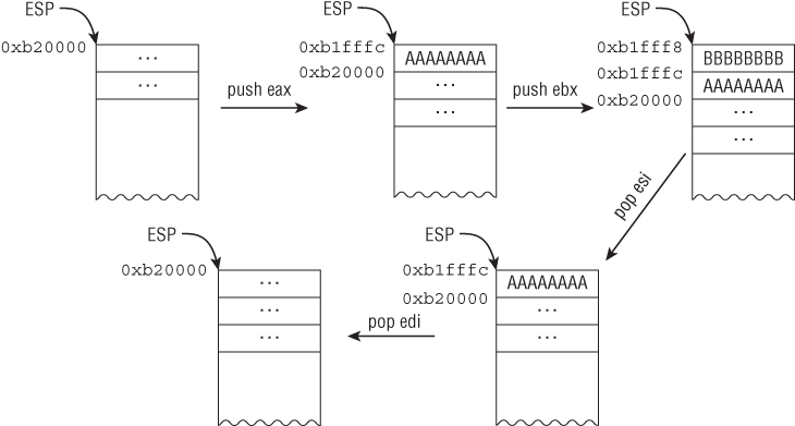
Suppose that ESP initially points to 0xb20000 and you have the following code:
; initial ESP = 0xb20000
01: B8 AA AA AA AA  mov    eax,0AAAAAAAAh
02: BB BB BB BB BB  mov    ebx,0BBBBBBBBh
03: B9 CC CC CC CC  mov    ecx,0CCCCCCCCh
04: BA DD DD DD DD  mov    edx,0DDDDDDDDh
05: 50              push   eax
; address 0xb1fffc will contain the value 0xAAAAAAAA and ESP
; will be 0xb1fffc (=0xb20000-4)
06: 53              push   ebx
; address 0xb1fff8 will contain the value 0xBBBBBBBB and ESP
; will be 0xb1fff8 (=0xb1fffc-4)
07: 5E              pop    esi
; ESI will contain the value 0xBBBBBBBB and ESP will be 0xb1fffc
; (=0xb1fff8+4)
08: 5F              pop    edi
; EDI will contain the value 0xAAAAAAAA and ESP will be 0xb20000
; (=0xb1fffc+4)
Figure 1.3 illustrates the stack layout.
ESP can also be directly modified by other instructions, such as ADD and SUB.
While high-level programming languages have the concept of functions that can be called and returned from, the processor does not provide such abstraction. At the lowest level, the processor operates only on concrete objects, such as registers or data coming from memory. How are functions translated at the machine level? They are implemented through the stack data structure! Consider the following function:
C
int
__cdecl addme(short a, short b)
{
    return a+b;
}
Assembly
01: 004113A0 55           push   ebp
02: 004113A1 8B EC        mov    ebp, esp
03: …
04: 004113BE 0F BF 45 08  movsx  eax, word ptr [ebp+8]
05: 004113C2 0F BF 4D 0C  movsx  ecx, word ptr [ebp+0Ch]
06: 004113C6 03 C1        add   eax, ecx
07: …
08: 004113CB 8B E5        mov    esp, ebp
09: 004113CD 5D           pop    ebp
10: 004113CE C3           retn
The function is invoked with the following code:
C
sum = addme(x, y);
Assembly
01: 004129F3 50               push  eax
02: …
03: 004129F8 51               push  ecx
04: 004129F9 E8 F1 E7 FF FF   call  addme
05: 004129FE 83 C4 08         add   esp, 8
Before going into the details, first consider the CALL/RET instructions and calling conventions. The CALL instruction performs two operations:
RET simply pops the address stored on the top of the stack into EIP and transfers control to it (literally like a “POP EIP” but such instruction sequence does not exist on x86). For example, if you want to begin execution at 0x12345678, you can just do the following:
01: 68 78 56 34 12   push  0x12345678
02: C3               ret
A calling convention is a set of rules dictating how function calls work at the machine level. It is defined by the Application Binary Interface (ABI) for a particular system. For example, should the parameters be passed through the stack, in registers, or both? Should the parameters be passed in from left-to-right or right-to-left? Should the return value be stored on the stack, in registers, or both? There are many calling conventions, but the popular ones are CDECL, STDCALL, THISCALL, and FASTCALL. (The compiler can also generate its own custom calling convention, but those will not be discussed here.) Table 1.2 summarizes their semantic.
Table 1.2 Calling Conventions
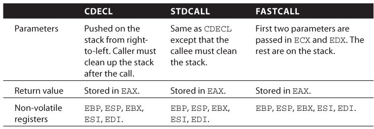
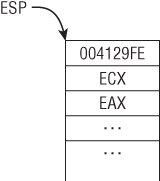
We now return to the code snippet to discuss how the function addme is invoked. In line 1 and 3, the two parameters are pushed on the stack; ECX and EAX are the first and second parameter, respectively. Line 4 invokes the addme function with the CALL instruction. This immediately pushes the return address, 0x4129FE, on the stack and begins execution at 0x4113A0. Figure 1.4 illustrates the stack layout after line 4 is executed.
After line 4 executes, we are now in the addme function body. Line 1 pushes EBP on the stack. Line 2 sets EBP to the current stack pointer. This two-instruction sequence is typically known as the function prologue because it establishes a new function frame. Line 4 reads the value at address EBP+8, which is the first parameter on the stack; line 5 reads the second parameter. Note that the parameters are accessed using EBP as the base register. When used in this context, EBP is known as the base frame pointer (see line 2) because it points to the stack frame for the current function, and parameters/locals can be accessed relative to it. The compiler can also be instructed to generate code that does not use EBP as the base frame pointer through an optimization called frame pointer omission. With such optimization, access to local variables and parameters is done relative to ESP, and EBP can be used as a general register like EAX, EBX, ECX, and so on. Line 6 adds the numbers and saves the result in EAX. Line 8 sets the stack pointer to the base frame pointer. Line 9 pops the saved EBP from line 1 into EBP. This two-instruction sequence is commonly referred to as the function epilogue because it is at the end of the function and restores the previous function frame. At this point, the top of the stack contains the return address saved by the CALL instruction at 0x4129F9. Line 10 performs a RET, which pops the stack and resumes execution at 0x4129FE. Line 5 in the snippet shrinks the stack by 8 because the caller must clean up the stack per CDECL's calling convention.
If the function addme had local variables, the code would need to grow the stack by subtracting ESP after line 2. All local variables would then be accessible through a negative offset from EBP.
This section describes how the system implements conditional execution for higher-level constructs like if/else, switch/case, and while/for. All of these are implemented through the CMP, TEST, JMP, and Jcc instructions and EFLAGS register. The following list summarizes the common flags in EFLAGS:
Arithmetic instructions update these flags based on the result. For example, the instruction SUB EAX, EAX would cause ZF to be set. The Jcc instructions, where “cc” is a conditional code, changes control flow depending on these flags. There can be up to 16 conditional codes, but the most common ones are described in Table 1.3.
Table 1.3 Common Conditional Codes
| Conditional Code | English Description | Machine Description |
| B/NAE | Below/Neither Above nor Equal. Used for unsigned operations. | CF=1 |
| NB/AE | Not Below/Above or Equal. Used for unsigned operations. | CF=0 |
| E/Z | Equal/Zero | ZF=1 |
| NE/NZ | Not Equal/Not Zero | ZF=0 |
| L | Less than/Neither Greater nor Equal. Used for signed operations. | (SF ^ OF) = 1 |
| GE/NL | Greater or Equal/Not Less than. Used for signed operations. | (SF ^ OF) = 0 |
| G/NLE | Greater/Not Less nor Equal. Used for signed operations. | ((SF ^ OF) | ZF) = 0 |
Because assembly language does not have a defined type system, one of the few ways to recognize signed/unsigned types is through these conditional codes.
The CMP instruction compares two operands and sets the appropriate conditional code in EFLAGS; it compares two numbers by subtracting one from another without updating the result. The TEST instruction does the same thing except it performs a logical AND between the two operands.
If-else constructs are quite simple to recognize because they involve a compare/test followed by a Jcc. For example:
Assembly
01:   mov   esi, [ebp+8]
02:   mov   edx, [esi]
03:   test  edx, edx
04:   jz    short loc_4E31F9
05:   mov   ecx, offset _FsRtlFastMutexLookasideList
06:   call  _ExFreeToNPagedLookasideList@8
07:   and   dword ptr [esi], 0
08:   lea   eax, [esi+4]
09:   push  eax
10:   call  _FsRtlUninitializeBaseMcb@4
11: loc_4E31F9:
12:   pop   esi
13:   pop   ebp
14:   retn  4
15: _FsRtlUninitializeLargeMcb@4 endp
Pseudo C
if (*esi == 0) {
  return;
}
ExFreeToNPagedLookasideList(…);
*esi = 0;
…
return;
OR
if (*esi != 0) {
  …
  ExFreeToNPagedLookasideList(…);
  *esi = 0;
  …
}
return;
Line 2 reads a value at location ESI and stores it in EDX. Line 3 ANDs EDX with itself and sets the appropriate flags in EFLAGS. Note that this pattern is commonly used to determine whether a register is zero. Line 4 jumps to loc_4E31F9 (line 12) if ZF=1. If ZF=0, then it executes line 5 and continues until the function returns.
Note that there are two slightly different but logically equivalent C translations for this snippet.
A switch-case block is a sequence of if/else statements. For example:
Switch-Case
switch(ch) {
    case 'c':
        handle_C();
        break;
    case 'h':
        handle_H();
        break;
    default:
        break;
}
domore();
…
If-Else
if (ch == 'c') {
    handle_C();
} else
if (ch == 'h') {
    handle_H();
}
domore();
…
Hence, the machine code translation will be a series if/else. The following simple example illustrates the idea:
Assembly
01:   push   ebp
02:   mov    ebp, esp
03:   mov    eax, [ebp+8]
04:   sub    eax, 41h
05:   jz     short loc_caseA
06:   dec    eax
07:   jz     short loc_caseB
08:   dec    eax
09:   jz     short loc_caseC
10:   mov    al, 5Ah
11:   movzx  eax, al
12:   pop    ebp
13:   retn
14: loc_caseC:
15:   mov    al, 43h
16:   movzx  eax, al
17:   pop    ebp
18:   retn
19: loc_caseB:
20:   mov    al, 42h
21:   movzx  eax, al
22:   pop    ebp
23:   retn
24: loc_caseA:
25:   mov    al, 41h
26:   movzx  eax, al
27:   pop    ebp
28:   retn
C
unsigned char switchme(int a)
{
    unsigned char res;
    switch(a) {
    case 0x41:
        res = 'A';
        break;
    case 0x42:
        res = 'B';
        break;
    case 0x43:
        res = 'C';
        break;
    default:
        res = 'Z';
        break;
    }
    return res;
}
Real-life switch-case statements can be more complex, and compilers commonly build a jump table to reduce the number of comparisons and conditional jumps. The jump table is essentially an array of addresses, each pointing to the handler for a specific case. This pattern can be observed in Sample J in sub_10001110:
Assembly
01:   cmp     edi, 5
02:   ja      short loc_10001141
03:   jmp     ds:off_100011A4[edi*4]
04: loc_10001125:
05:   mov     esi, 40h
06:   jmp     short loc_10001145
07: loc_1000112C:
08:   mov     esi, 20h
09:   jmp     short loc_10001145
10: loc_10001133:
11:   mov     esi, 38h
12:   jmp     short loc_10001145
13: loc_1000113A:
14:   mov     esi, 30h
15:   jmp     short loc_10001145
16: loc_10001141:
17:   mov     esi, [esp+0Ch]
18: …
19: off_100011A4 dd offset loc_10001125
20:   dd offset loc_10001125
21:   dd offset loc_1000113A
22:   dd offset loc_1000112C
23:   dd offset loc_10001133
24:   dd offset loc_1000113A
Pseudo C
switch(edi) {
  case 0:
  case 1:
    // goto loc_10001125;
    esi = 0x40;
    break;
  case 2:
  case 5:
    // goto loc_1000113A;
    esi = 0x30;
    break;
  case 3:
    // goto loc_1000112C;
    esi = 0x20;
    break;
  case 4:
    // goto loc_10001133;
    esi = 0x38;
    break;
  default:
    // goto loc_10001141;
    esi = *(esp+0xC)
    break;
}
…
Here, the compiler knows that there are only five cases and the case value is consecutive; hence, it can construct the jump table and index into it directly (line 3). Without the jump table, there would be 10 additional instructions to test each case and branch to the handler. (There are other forms of switch/case optimizations, but we will not cover them here.)
At the machine level, loops are implemented using a combination of Jcc and JMP instructions. In other words, they are implemented using if/else and goto constructs. The best way to understand this is to rewrite a loop using only if/else and goto. Consider the following example:
Using for
for (int i=0; i<10; i++) {
    printf("%d\n", i);
}
printf("done!\n");
Using if/else and goto
int i = 0;
loop_start:
    if (i < 10) {
        printf("%d\n", i);
        i++;
        goto loop_start;
    }
printf("done!n");
When compiled, both versions are identical at the machine-code level:
01: 00401002   mov    edi, ds:__imp__printf
02: 00401008   xor    esi, esi
03: 0040100A   lea    ebx, [ebx+0]
04: 00401010 loc_401010:
05: 00401010   push   esi
06: 00401011   push   offset Format                 ; "%d\n"
07: 00401016   call   edi ; __imp__printf
08: 00401018   inc    esi
09: 00401019   add    esp, 8
10: 0040101C   cmp    esi, 0Ah
11: 0040101F   jl     short loc_401010
12: 00401021   push   offset aDone                  ; "done!\n"
13: 00401026   call   edi ; __imp__printf
14: 00401028   add    esp, 4
Line 1 sets EDI to the printf function. Line 2 sets ESI to 0. Line 4 begins the loop; however, note that it does not begin with a comparison. There is no comparison here because the compiler knows that the counter was initialized to 0 (see line 2) and is obviously going to be less than 10 so it skips the check. Lines 5–7 call the printf function with the right parameters (format specifier and our number). Line 8 increments the number. Line 9 cleans up the stack because printf uses the CDECL calling convention. Line 10 checks to see if the counter is less than 0xA. If it is, it jumps back to loc_401010. If the counter is not less than 0xA, it continues execution at line 12 and finishes with a printf.
One important observation to make is that the disassembly allowed us to infer that the counter is a signed integer. Line 11 uses the “less than” conditional code (JL), so we immediately know that the comparison was done on signed integers. Remember: If “above/below,” it is unsigned; if “less than/greater than,” it is signed. Sample L has a small function, sub_1000AE3B, with the following interesting loop:
Assembly
01: sub_1000AE3B proc near
02:   push    edi
03:   push    esi
04:   call    ds:lstrlenA
05:   mov     edi, eax
06:   xor     ecx, ecx
07:   xor     edx, edx
08:   test    edi, edi
09:   jle     short loc_1000AE5B
10: loc_1000AE4D:
11:   mov     al, [edx+esi]
12:   mov     [ecx+esi], al
13:   add     edx, 3
14:   inc     ecx
15:   cmp     edx, edi
16:   jl      short loc_1000AE4D
17: loc_1000AE5B:
18:   mov     byte ptr [ecx+esi], 0
19:   mov     eax, esi
20:   pop     edi
21:   retn
22: sub_1000AE3B endp
C
char *sub_1000AE3B (char *str)
{
  int len, i=0, j=0;
  len = lstrlenA(str);
  if (len <= 0) {
    str[j] = 0;
    return str;
  }
  while (j < len) {
    str[i] = str[j];
    j = j+3;
    i = i+1;
  }
  str[i] = 0;
  return str;
}
The sub_1000AE3B function has one parameter passed using a custom calling convention (ESI holds the parameter). Line 2 saves EDI. Line 3 calls lstrlenA with the parameter; hence, you immediately know that ESI is of type char *. Line 5 saves the return value (string length) in EDI. Lines 6–7 clear ECX and EDX. Lines 8–9 check to see if the string length is less than or equal to zero. If it is, control is transferred to line 18, which sets the value at ECX+ESI to 0. If it is not, then execution is continued at line 11, which is the start of a loop. First, it reads the character at ESI+EDX (line 11), and then it stores it at ESI+ECX (line 12). Next, it increments the EDX and ECX by three and one, respectively. Lines 15–16 check to see if EDX is less than the string length; if so, execution goes back to the loop start. If not, execution is continued at line 18.
It may seem convoluted at first, but this function takes an obfuscated string whose deobfuscated value is every third character. For example, the string SX]OTYFKPTY^W\\aAFKRW\\E is actually SOFTWARE. The purpose of this function is to prevent naïve string scanners and evade detection. As an exercise, you should decompile this function so that it looks more “natural” (as opposed to our literal translation).
Outside of the normal Jcc constructs, certain loops can be implemented using the LOOP instruction. The LOOP instruction executes a block of code up to ECX time. For example:
Assembly
01: 8B CA         mov    ecx, edx
02:             loc_CFB8F:
03: AD            lodsd
04: F7 D0         not    eax
05: AB            stosd
06: E2 FA         loop   loc_CFB8F
Rough C
while (ecx != 0) {
    eax = *edi;
    edi++;
    *esi = ∼eax;
    esi++;
    ecx--;
}
Line 1 reads the counter from EDX. Line 3 is the loop start; it reads in a double-word at the memory address EDI and saves that in EAX; it also increments EDI by 4. Line 4 performs the NOT operator on the value just read. Line 5 writes the modified value to the memory address ESI and increments ESI by 4. Line 6 checks to see if ECX is 0; if not, execution is continued at the loop start.
The previous sections explain mechanisms and instructions that are available to code running at all privilege levels. To get a better appreciation of the architecture, this section discusses two fundamental system-level mechanisms: virtual address translation and exception/interrupt handling. You may skip this section on a first read.
The physical memory on a computer system is divided into 4KB units called pages. (A page can be more than 4KB, but we will not discuss the other sizes here.) Memory addresses are divided into two categories: virtual and physical. Virtual addresses are those used by instructions executed in the processor when paging is enabled. For example:
01: A1 78 56 34 12  mov   eax, [0x12345678]; read memory at the virtual
                                           ; address 0x12345678
01: 89 08           mov   [eax], ecx       ; write ECX at the virtual
                                           ; address EAX
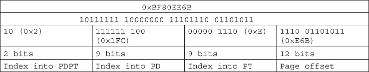
Physical addresses are the actual memory locations used by the processor when accessing memory. The processor's memory management unit (MMU) transparently translates every virtual address into a physical address before accessing it. While a virtual address may seem like just another number to the user, there is a structure to it when viewed by the MMU. On x86 systems with physical address extension (PAE) support, a virtual memory address can be divided into indices into three tables and offset: page directory pointer table (PDPT), page directory (PD), page table (PT), and page table entry (PTE). A PDPT is an array of four 8-byte elements, each pointing to a PD. A PD is an array of 512 8-byte elements, each pointing to a PT. A PT is an array of 512 8-byte elements each containing a PTE. For example, the virtual address 0xBF80EE6B can be understood as shown in Figure 1.5.
The 8-byte elements in these tables contain data about the tables, memory permission, and other memory characteristics. For example, there are bits that determine whether the page is read-only or readable/writable, executable or non-executable, accessible by user or not, and so on.
The address translation process revolves around these three tables and the CR3 register. CR3 holds the physical base address of the PDPT. The rest of this section walks through the translation of the virtual address 0xBF80EE6B on a real system (refer to Figure 1.5):
kd> r @cr3           ; CR3 is the physical address for the base of a PDPT
cr3=085c01e0
kd> !dq @cr3+2*8 L1  ; read the PDPT entry at index 2
# 85c01f0 00000000`0d66e001
Per the documentation, the bottom 12 bits of a PDPT entry are flags/reserved bits, and the remaining ones are used as the physical address of the PD base. Bit 63 is the NX flag in PAE, so you will also need to clear that as well. In this particular example, we did not clear it because it is already 0. (We are looking at code pages that are executable.)
; 0x00000000`0d66e001 = 00001101 01100110 11100000 00000001
; after clearing the bottom 12 bits, we have
; 0x0d66e000          = 00001101 01100110 11100000 00000000
; This tells us that the PD base is at physical address 0x0d66e000
kd> !dq 0d66e000+0x1fc*8 L1   ; read the PD entry at index 0x1FC
# d66efe0 00000000`0964b063
Again, per the documentation, the bottom 12 bits of a PD entry are used for flags/reserved bits, and the remaining ones are used as the base for the PT:
; 0x0964b063 = 00001001 01100100 10110000 01100011
; after clearing the bottom 12 bits, we get
; 0x0964b000 = 00001001 01100100 10110000 00000000
; This tells us that the PT base is at 0x0964b000
kd> !dq 0964b000+e*8 L1      ; read the PT entry at index 0xE
# 964b070 00000000`06694021
Again, the bottom 12 bits can be cleared to get to the base of a page entry:
; 0x06694021 = 00000110 01101001 01000000 00100001
; after clearing bottom 12 bits, we get
; 0x06694000 = 00000110 01101001 01000000 00000000
; This tells us that the page entry base is at 0x06694000
kd> !db 06694000+e6b L8      ; read 8 bytes from the page entry at offset 0xE6B
# 6694e6b 8b ff 55 8b ec 83 ec 0c ..U.....[).t....    ; our data at that
                                                      ; physical page
kd> db bf80ee6b L8           ; read 8 bytes from the virtual address
bf80ee6b  8b ff 55 8b ec 83 ec ..U.....[).t....       ; same data!
After the entire process, it is determined that the virtual address 0xBF80EE6B translates to the physical address 0x6694E6B.
Modern operating systems implement process address space separation using this mechanism. Every process is associated with a different CR3, resulting in process-specific virtual address translation. It is the magic behind each process's illusion that it has its own address space. Hopefully you will have more appreciation for the processor the next time your program accesses memory!
This section briefly discusses interrupts and exceptions, as complete implementation details can be found in Chapter 3, “The Windows Kernel.”
In contemporary computing systems, the processor is typically connected to peripheral devices through a data bus such as PCI Express, FireWire, or USB. When a device requires the processor's attention, it causes an interrupt that forces the processor to pause whatever it is doing and handle the device's request. How does the processor know how to handle the request? At the highest level, one can think of an interrupt as being associated with a number that is then used to index into an array of function pointers. When the processor receives the interrupt, it executes the function at the index associated with the interrupt and resumes execution at wherever it was before the interrupt occurred. These are called hardware interrupts because they are generated by hardware devices. They are asynchronous by nature.
When the processor is executing an instruction, it may run into exceptions. For example, an instruction could generate a divide-by-zero error, reference an invalid address, or trigger a privilege level transition. For the purpose of this discussion, exceptions can be classified into two categories: faults and traps. A fault is a correctable exception. For example, when the processor executes an instruction that references a valid memory address but the data is not present in main memory (it was paged out), a page fault exception is generated. The processor handles this by saving the current execution state, calling the page fault handler to correct this exception (by paging in the data), and re-executing the same instruction (which should no longer cause a page fault). A trap is an exception caused by executing special kinds of instructions. For example, the instruction SYSENTER causes the processor to begin executing the generic system call handler; after the handler is done, execution is resumed at the instruction immediately after SYSENTER. Hence, the major difference between a fault and a trap is where execution resumes. Operating systems commonly implement system calls through the interrupt and exception mechanism.
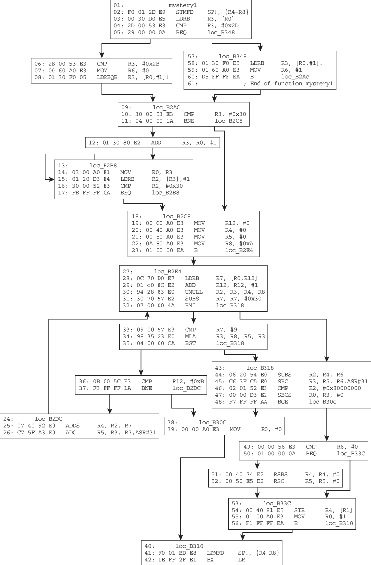
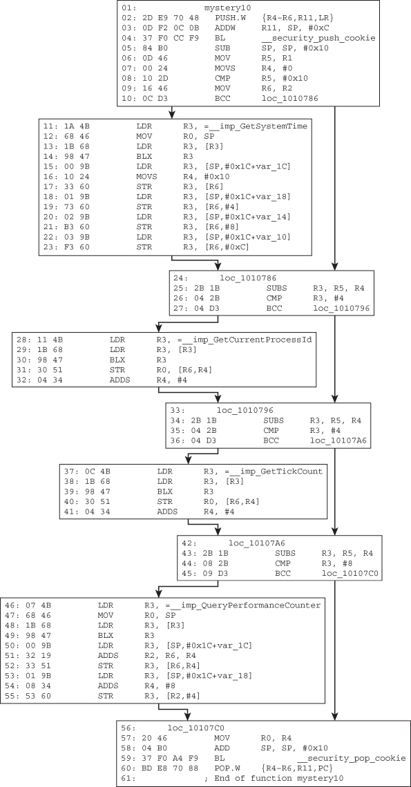
We finish the chapter with a walk-through of a function with fewer than 100 instructions. It is Sample J's DllMain routine. This exercise has two objectives. First, it applies almost every concept covered in the chapter (except for switch-case). Second, it teaches an important requirement in the practice of reverse engineering: reading technical manuals and online documentation. Here is the function:
01:    ; BOOL __stdcall DllMain(HINSTANCE hinstDLL, DWORD fdwReason,
       ; LPVOID lpvReserved)
02:                _DllMain@12 proc near
03: 55               push    ebp
04: 8B EC            mov     ebp, esp
05: 81 EC 30 01 00+  sub     esp, 130h
06: 57               push    edi
07: 0F 01 4D F8      sidt    fword ptr [ebp-8]
08: 8B 45 FA         mov     eax, [ebp-6]
09: 3D 00 F4 03 80   cmp     eax, 8003F400h
10: 76 10            jbe     short loc_10001C88 (line 18)
11: 3D 00 74 04 80   cmp     eax, 80047400h
12: 73 09            jnb     short loc_10001C88 (line 18)
13: 33 C0            xor     eax, eax
14: 5F               pop     edi
15: 8B E5            mov     esp, ebp
16: 5D               pop     ebp
17: C2 0C 00         retn    0Ch
18:                loc_10001C88:
19: 33 C0            xor     eax, eax
20: B9 49 00 00 00   mov     ecx, 49h
21: 8D BD D4 FE FF+  lea     edi, [ebp-12Ch]
22: C7 85 D0 FE FF+  mov     dword ptr [ebp-130h], 0
23: 50               push    eax
24: 6A 02            push    2
25: F3 AB            rep stosd
26: E8 2D 2F 00 00   call    CreateToolhelp32Snapshot
27: 8B F8            mov     edi, eax
28: 83 FF FF         cmp     edi, 0FFFFFFFFh
29: 75 09            jnz     short loc_10001CB9 (line 35)
30: 33 C0            xor     eax, eax
31: 5F               pop     edi
32: 8B E5            mov     esp, ebp
33: 5D               pop     ebp
34: C2 0C 00         retn    0Ch
35:                loc_10001CB9:
36: 8D 85 D0 FE FF+  lea     eax, [ebp-130h]
37: 56               push    esi
38: 50               push    eax
39: 57               push    edi
40: C7 85 D0 FE FF+  mov     dword ptr [ebp-130h], 128h
41: E8 FF 2E 00 00   call    Process32First
42: 85 C0            test    eax, eax
43: 74 4F            jz      short loc_10001D24 (line 70)
44: 8B 35 C0 50 00+  mov     esi, ds:_stricmp
45: 8D 8D F4 FE FF+  lea     ecx, [ebp-10Ch]
46: 68 50 7C 00 10   push    10007C50h
47: 51               push    ecx
48: FF D6            call    esi ; _stricmp
49: 83 C4 08         add     esp, 8
50: 85 C0            test    eax, eax
51: 74 26            jz      short loc_10001D16 (line 66)
52:                loc_10001CF0:
53: 8D 95 D0 FE FF+  lea     edx, [ebp-130h]
54: 52               push    edx
55: 57               push    edi
56: E8 CD 2E 00 00   call    Process32Next
57: 85 C0            test    eax, eax
58: 74 23            jz      short loc_10001D24 (line 70)
59: 8D 85 F4 FE FF+  lea     eax, [ebp-10Ch]
60: 68 50 7C 00 10   push    10007C50h
61: 50               push    eax
62: FF D6            call    esi ; _stricmp
63: 83 C4 08         add     esp, 8
64: 85 C0            test    eax, eax
65: 75 DA            jnz     short loc_10001CF0 (line 52)
66:                loc_10001D16:
67: 8B 85 E8 FE FF+  mov     eax, [ebp-118h]
68: 8B 8D D8 FE FF+  mov     ecx, [ebp-128h]
69: EB 06            jmp     short loc_10001D2A (line 73)
70:                loc_10001D24:
71: 8B 45 0C         mov     eax, [ebp+0Ch]
72: 8B 4D 0C         mov     ecx, [ebp+0Ch]
73:                loc_10001D2A:
74: 3B C1            cmp     eax, ecx
75: 5E               pop     esi
76: 75 09            jnz     short loc_10001D38 (line 82)
77: 33 C0            xor     eax, eax
78: 5F               pop     edi
79: 8B E5            mov     esp, ebp
80: 5D               pop     ebp
81: C2 0C 00         retn    0Ch
82:                loc_10001D38:
83: 8B 45 0C         mov     eax, [ebp+0Ch]
84: 48               dec     eax
85: 75 15            jnz     short loc_10001D53 (line 93)
86: 6A 00            push    0
87: 6A 00            push    0
88: 6A 00            push    0
89: 68 D0 32 00 10   push    100032D0h
90: 6A 00            push    0
91: 6A 00            push    0
92: FF 15 20 50 00+  call    ds:CreateThread
93:                loc_10001D53:
94: B8 01 00 00 00   mov     eax, 1
95: 5F               pop     edi
96: 8B E5            mov     esp, ebp
97: 5D               pop     ebp
98: C2 0C 00         retn    0Ch
99:                _DllMain@12 endp
Lines 3–4 set up the function prologue, which saves the previous base frame pointer and establishes a new one. Line 5 reserves 0x130 bytes of stack space. Line 6 saves EDI. Line 7 executes the SIDT instruction, which writes the 6-byte IDT register to a specified memory region. Line 8 reads a double-word at EBP-6 and saves it in EAX. Lines 9–10 check if EAX is below-or-equal to 0x8003F400. If it is, execution is transferred to line 18; otherwise, it continues executing at line 11. Lines 11–12 do a similar check except that the condition is not-below 0x80047400. If it is, execution is transferred to line 18; otherwise, it continues executing at line 13. Line 13 clears EAX. Line 14 restores the saved EDI register in line 6. Lines 15–16 restore the previous base frame and stack pointer. Line 17 adds 0xC bytes to the stack pointer and then returns to the caller.
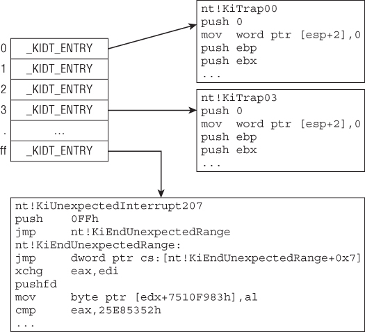
Before discussing the next area, note a few things about these first 17 lines. The SIDT instruction (line 7) writes the content of the IDT register to a 6-byte memory location. What is the IDT register? The Intel/AMD reference manual states that IDT is an array of 256 8-byte entries, each containing a pointer to an interrupt handler, segment selector, and offset. When an interrupt or exception occurs, the processor uses the interrupt number as an index into the IDT and calls the entry's specified handler. The IDT register is a 6-byte register; the top 4 bytes contain the base of the IDT array/table and the bottom 2 bytes store the table limit. With this in mind, you now know that line 8 is actually reading the IDT base address. Lines 9 and 11 check whether the base address is in the range (0x8003F400, 0x80047400). What is special about these seemingly random constants? If you search the Internet, you will note that 0x8003F400 is an IDT base address on Windows XP on x86. This can be verified in the kernel debugger:
0: kd> vertarget
Windows XP Kernel Version 2600 (Service Pack 3) MP (2 procs) Free x86 compatible
Built by: 2600.xpsp.080413-2111
…
0: kd> r @idtr
idtr=8003f400
0: kd> ∼1
1: kd> r @idtr
idtr=bab3c590
Why does the code check for this behavior? One possible explanation is that the developer assumed that an IDT base address falling in that range is considered “invalid” or may be the result of being virtualized. The function automatically returns zero if the IDTR is “invalid.” You can decompile this code to C as follows:
typedef struct _IDTR {
    DWORD base;
    SHORT limit;
} IDTR, *PIDTR;
BOOL __stdcall DllMain (HINSTANCE hinstDLL, DWORD fdwReason, LPVOID lpvReserved)
{
    IDTR idtr;
    __sidt(&idtr);
    if (idtr.base > 0x8003F400 && idtr.base < 0x80047400h) { return FALSE; }
    //line 18
    …
}
If the IDT base seems valid, the code continues execution at line 18. Lines 19–20 clear EAX and set ECX to 0x49. Line 21 uses sets EDI to whatever EBP-0x12C is; since EBP is the base frame pointer, EBP-0x12C is the address of a local variable. Line 22 writes zero at the location pointed to by EBP-0x130. Lines 23–24 push EAX and 2 on the stack. Line 25 zeroes a 0x124-byte buffer starting from EBP-0x12C. Line 26 calls CreateToolhelp32Snapshot:
HANDLE WINAPI CreateToolhelp32Snapshot(
  _In_ DWORD dwFlags,
  _In_ DWORD th32ProcessID
);
This Win32 API function takes two integer parameters. As a general rule, Win32 API functions follow STDCALL calling convention. Hence, the dwFlags and th32ProcessId parameters are 0x2 (line 24) and 0x0 (line 23). This function enumerates all processes on the system and returns a handle to be used in Process32Next. Lines 27–28 save the return value in EDI and check if it is -1. If it is, the return value is set to 0 and it returns (lines 30–34); otherwise, execution continues at line 35. Line 36 sets EAX to the address of the local variable previously initialized to 0 in line 22; line 40 initializes it to 0x128. Lines 37–39 push ESI, EAX, and EDI on the stack. Line 41 calls Process32First:
Function prototype
BOOL WINAPI Process32First(
  _In_     HANDLE hSnapshot,
  _Inout_  LPPROCESSENTRY32 lppe
);
Relevant structure definition
typedef struct tagPROCESSENTRY32 {
  DWORD     dwSize;
  DWORD     cntUsage;
  DWORD     th32ProcessID;
  ULONG_PTR th32DefaultHeapID;
  DWORD     th32ModuleID;
  DWORD     cntThreads;
  DWORD     th32ParentProcessID;
  LONG      pcPriClassBase;
  DWORD     dwFlags;
  TCHAR     szExeFile[MAX_PATH];
} PROCESSENTRY32, *PPROCESSENTRY32;
00000000 PROCESSENTRY32 struc ; (sizeof=0x128)
00000000 dwSize dd ?
00000004 cntUsage dd ?
00000008 th32ProcessID dd ?
0000000C th32DefaultHeapID dd ?
00000010 th32ModuleID dd ?
00000014 cntThreads dd ?
00000018 th32ParentProcessID dd ?
0000001C pcPriClassBase dd ?
00000020 dwFlags dd ?
00000024 szExeFile db 260 dup(?)
00000128 PROCESSENTRY32 ends
Because this API takes two parameters, hSnapshot is EDI (line 39, previously the returned handle from CreateToolhelp32Snapshot in line 27), and lppe is the address of a local variable (EBP-0x130). Because lppe points to a PROCESSENTRY32 structure, we immediately know that the local variable at EBP-0x130 is of the same type. It also makes sense because the documentation for Process32First states that before calling the function, the dwSize field must be set to the size of a PROCESSENTRY32 structure (which is 0x128). We now know that lines 19–25 were simply initializing this structure to 0. In addition, we can say that this local variable starts at EBP-0x130 and ends at EBP-0x8.
Line 42 tests the return value of Process32Next. If it is zero, execution begins at line 70; otherwise, it continues at line 43. Line 44 saves the address of the stricmp function in ESI. Line 45 sets ECX to the address of a local variable (EBP-0x10C), which happens to be a field in PROCESSENTRY32 (see the previous paragraph). Lines 46–48 push 0x10007C50/ECX on the stack and call stricmp. We know that stricmp takes two character strings as arguments; hence, ECX must be the szExeFile field in PROCESSENTRY32 and 0x10007C50 is the address of a string:
.data:10007C50 65 78 70 6C 6F+Str2 db 'explorer.exe',0
Line 49 cleans up the stack because stricmp uses CDECL calling convention. Line 50 checks stricmp's return value. If it is zero, meaning that the string matched “explorer.exe”, execution begins at line 66; otherwise, it continues execution at line 52. We can now decompile lines 18–51 as follows:
    HANDLE h;
    PROCESSENTRY32 procentry;
    h = CreateToolhelp32Snapshot(TH32CS_SNAPPROCESS, 0);
    if (h == INVALID_HANDLE_VALUE) { return FALSE; }
    memset(&procentry, 0, sizeof(PROCESSENTRY32));
    procentry.dwSize = sizeof(procentry); // 0x128
    if (Process32Next(h, &procentry) == FALSE) {
        // line 70
        …
    }
    if (stricmp(procentry.szExeFile, "explorer.exe") == 0) {
        // line 66
        …
    }
    // line 52
Lines 52–65 are nearly identical to the previous block except that they form a loop with two exit conditions. The first exit condition is when Process32Next returns FALSE (line 58) and the second is when stricmp returns zero. We can decompile lines 52–65 as follows:
    while (Process32Next(h, &procentry) != FALSE) {
        if (stricmp(procentry.szExeFile, "explorer".exe") == 0)
            break;
    }
After the loop exits, execution resumes at line 66. Lines 67–68 save the matching PROCESSENTRY32's th32ParentProcessID/th32ProcessID in EAX/ECX and continue execution at 37. Notice that Line 66 is also a jump target in line 43.
Lines 70–74 read the fdwReason parameter of DllMain (EBP+C) and check whether it is 0 (DLL_PROCESS_DETACH). If it is, the return value is set to 0 and it returns; otherwise, it goes to line 82. Lines 82–85 check if the fdwReason is greater than 1 (i.e., DLL_THREAD_ATTACH, DLL_THREAD_DETACH). If it is, the return value is set to 1 and it returns; otherwise, execution continues at line 86. Lines 86–92 call CreateThread:
HANDLE WINAPI CreateThread(
  _In_opt_   LPSECURITY_ATTRIBUTES lpThreadAttributes,
  _In_       SIZE_T dwStackSize,
  _In_       LPTHREAD_START_ROUTINE lpStartAddress,
  _In_opt_   LPVOID lpParameter,
  _In_       DWORD dwCreationFlags,
  _Out_opt_  LPDWORD lpThreadId
);
with lpStartAddress as 0x100032D0. This block can be decompiled as follows:
if (fdwReason == DLL_PROCESS_DETACH) { return FALSE; }
if (fdwReason == DLL_THREAD_ATTACH || fdwReason == DLL_THREAD_DETACH) {
   return TRUE; }
CreateThread(0, 0, (LPTHREAD_START_ROUTINE) 0x100032D0, 0, 0, 0);
return TRUE;
Having analyzed the function, we can deduce that the developer's original intention was this:
x64 is an extension of x86, so most of the architecture properties are the same, with minor differences such as register size and some instructions are unavailable (like PUSHAD). The following sections discuss the relevant differences.
The register set has 18 64-bit GPRs, and can be illustrated as shown in Figure 1.6. Note that 64-bit registers have the “R” prefix.
While RBP can still be used as the base frame pointer, it is rarely used for that purpose in real-life compiler-generated code. Most x64 compilers simply treat RBP as another GPR, and reference local variables relative to RSP.
x64 supports a concept referred to as RIP-relative addressing, which allows instructions to reference data at a relative position to RIP. For example:
01: 0000000000000000 48 8B 05 00 00+  mov     rax, qword ptr cs:loc_A
02:                                   ; originally written as "mov rax, [rip]"
03: 0000000000000007                loc_A:
04: 0000000000000007 48 31 C0         xor     rax, rax
05: 000000000000000A 90               nop
Line 1 reads the address of loc_A (which is 0x7) and saves it in RAX. RIP-relative addressing is primarily used to facilitate position-independent code.
Most arithmetic instructions are automatically promoted to 64 bits even though the operands are only 32 bits. For example:
48 B8 88 77 66+ mov   rax, 1122334455667788h
31 C0           xor   eax, eax  ; will also clear the upper 32bits of RAX.
                                ; i.e., RAX=0 after this
48 C7 C0 FF FF+ mov   rax,0FFFFFFFFFFFFFFFFh
FF C0           inc   eax  ; RAX=0 after this
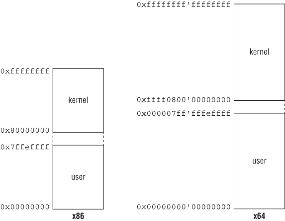
On x64, virtual addresses are 64 bits in width, but most processors do not support a full 64-bit virtual address space. Current Intel/AMD processors only use 48 bits for the address space. All virtual memory addresses must be in canonical form. A virtual address is in canonical form if bits 63 to the most significant implemented bit are either all 1s or 0s. In practical terms, it means that bits 48–63 need to match bit 47. For example:
0xfffff801`c9c11000 = 11111111 11111111 11111000 00000001 11001001 11000001
   00010000 00000000 ; canonical
0x000007f7`bdb67000 = 00000000 00000000 00000111 11110111 10111101 10110110
   01110000 00000000 ; canonical
0xffff0800`00000000 = 11111111 11111111 00001000 00000000 00000000 00000000
   00000000 00000000 ; non-canonical
0xffff8000`00000000 = 11111111 11111111 10000000 00000000 00000000 00000000
   00000000 00000000 ; canonical
0xfffff960`000989f0 = 11111111 11111111 11111001 01100000 00000000 00001001
   10001001 11110000 ; canonical
If code tries to dereference a non-canonical address, the system will cause an exception.
Recall that some calling conventions require parameters to be passed on the stack on x86. On x64, most calling conventions pass parameters through registers. For example, on Windows x64, there is only one calling convention and the first four parameters are passed through RCX, RDX, R8, and R9; the remaining are pushed on the stack from right to left. On Linux, the first six parameters are passed on RDI, RSI, RDX, RCX, R8, and R9.
A company named Acorn Computers developed a 32-bit RISC architecture named the Acorn RISC Machine (later renamed to Advanced RISC Machine) in the late 1980s. This architecture proved to be useful beyond their limited product line, so a company named ARM Holdings was formed to license the architecture for use in a wide variety of products. It is commonly found in embedded devices such as cell phones, automobile electronics, MP3 players, televisions, and so on. The first version of the architecture was introduced in 1985, and at the time of this writing it is at version 7 (ARMv7). ARM has developed a number of specific cores (e.g., ARM7, ARM7TDMI, ARM926EJS, Cortex)—not to be confused with the different architecture specifications, which are numbered ARMv1–ARMv7. While there are several versions, most devices are either on ARMv4, 5, 6, or 7. ARMv4 and v5 are relatively “old,” but they are also the most dominant and common versions of the processor (“more than 10 billion” cores in existence, according to ARM marketing). Popular consumer electronic products typically use more recent versions of the architecture. For example, the third-generation Apple iPod Touch and iPhone run on an ARMv6 chip, and later iPhone/iPad and Windows Phone 7 devices are all on ARMv7.
Whereas companies such as Intel and AMD design and manufacture their processors, ARM follows a slightly different model. ARM designs the architecture and licenses it to other companies, which then manufacture and integrate the processors into their devices. Companies such as Apple, NVIDIA, Qualcomm, and Texas Instruments market their own processors (A, Tegra, Snapdragon, and OMAP, respectively), but their core architecture is licensed from ARM. They all implement the base instruction set and memory model defined in the ARM architecture reference manual. Additional extensions can be added to the processor; for example, the Jazelle extension enables Java bytecode to be executed natively on the processor. The Thumb extension adds instructions that can be 16 or 32 bits wide, thus allowing higher code density (native ARM instructions are always 32 bits in width). The Debug extension allows engineers to analyze the physical processor using special debugging hardware. Each extension is typically represented by a letter (J, T, D, etc.). Depending on their requirements, manufacturers can decide whether they need to license these additional extensions. This is why ARMv6 and earlier processors have letters after them (e.g., ARM1156T2 means ARMv6 with Thumb-2 extension). These conventions are no longer used in ARMv7, which instead uses three profiles (Application, Real-time, and Microcontroller) and model name (Cortex) with different features. For example, ARMv7 Cortex-A series are processors with the application profile; and Cortex-M are meant for microcontrollers and only support Thumb mode execution.
This chapter covers the ARMv7 architecture as defined in the ARM Architecture Reference Manual: ARMv7-A and ARMv7-R Edition (ARM DDI 0406B).
Because ARM is a RISC architecture, there are a few basic differences between ARM and CISC architectures (x86/x64). (From a practical perspective, new versions of Intel processors have some RISC features as well—i.e., they are not “purely” CISC.) First, the ARM instruction set is very small compared to x86, but it offers more general-purpose registers. Second, the instruction length is fixed width (16 bits or 32 bits, depending on the state). Third, ARM uses a load-store model for memory access. This means data must be moved from memory into registers before being operated on, and only load/store instructions can access memory. On ARM, this translates to the LDR and STR instructions. If you want to increment a 32-bit value at a particular memory address, you must first load the value at that address to a register, increment it, and store it back. In contrast with x86, which allows most instructions to directly operate on data in memory, such a simple operation on ARM would require three instructions (one load, one increment, one store). This may imply that there is more code to read for the reverse engineer, but in practice it does not really matter much once you are used to it.
ARM also offers several different privilege levels to implement privilege isolation. In x86, privileges are defined by four rings, with ring 0 having the highest privilege and ring 3 having the lowest. In ARM, privileges are defined by eight different modes:
Code running in a given mode has access to certain privileges and registers that others may not; for example, code running in USR mode is not allowed to modify system registers (which are typically modified only in SVC mode). USR is the least privileged mode. While there are many technical differences, for the sake of simplicity you can make the analogy that USR is like ring 3 and SVC is like ring 0. Most operating systems implement kernel mode in SVC and user mode in USR. Both Windows and Linux do this.
If you recall from Chapter 1, x64 processors can execute in 32-bit, 64-bit, or both interchangeably. ARM processors are similar in that they can also operate in two states: ARM and Thumb. ARM/Thumb state determines only the instruction set, not the privilege level. For example, code running in SVC mode can be either ARM or Thumb. In ARM state, instructions are always 32 bits wide; in Thumb state, instructions can be either 16 bits or 32 bits wide. Which state the processor executes in depends on two conditions:
When an ARM core boots up, most of the time it enters ARM state and remains that way until there is an explicit or implicit change to Thumb. In practice, many recent operating system code mainly uses Thumb code because higher code density is wanted (a mixture of 16/32-bit wide instructions may be smaller in size than all 32-bit ones); applications can operate in whatever mode they want. While most Thumb and ARM instructions have the same mnemonic, 32-bit Thumb instructions have a .W suffix.
In addition to having different states of execution, ARM also supports conditional execution. This means that an instruction encodes certain arithmetic conditions that must be met in order for it to be executed. For example, an instruction can specify that it will only be executed if the result of the previous instruction is zero. Contrast this with x86, for which almost every single instruction is executed unconditionally. (Intel has a couple of instructions directly supporting conditional execution: CMOV and SETNE.) Conditional execution is useful because it cuts down on branch instructions (which are very expensive) and reduces the number of instructions to be executed (which leads to higher code density). All instructions in ARM state support conditional execution, but by default they execute unconditionally. In Thumb state, a special instruction IT is required to enable conditional execution.
Another unique ARM feature is the barrel shifter. Certain instructions can “contain” another arithmetic instruction that shifts or rotates a register. This is useful because it can shrink multiple instructions into one; for example, you want to multiply a register by 2 and then store the result in another register. Normally, this would require two instructions (a multiply followed by a move), but with the barrel shifter you can include the multiply (shift left by 1) inside the MOV instruction. The instruction would be something like the following:
MOV R1, R0, LSL #1 ; R1 = R0 * 2
Similar to high-level languages, ARM supports operations on different data types. The supported data types are: 8-bit (byte), 16-bit (half-word), 32-bit (word), and 64-bit (double-word).
The ARM architecture defines sixteen 32-bit general-purpose registers, numbered R0, R1, R2, . . . , R15. While all of them are available to the application programmer, in practice the first 12 registers are for general-purpose usage (such as EAX, EBX, etc., in x86) and the last three have special meaning in the architecture:
1: 0x00008344 push    {lr}
2: 0x00008346 mov     r0, pc
3: 0x00008348 mov.w   r2, r1, lsl #31
4: 0x0000834c pop     {pc}
After line 2 is executed, R0 will hold the value 0x0000834a (=0x00008346+4):
(gdb) br main
Breakpoint 1 at 0x8348
…
Breakpoint 1, 0x00008348 in main ()
(gdb) disas main
Dump of assembler code for function main:
   0x00008344 <+0>:     push    {lr}
   0x00008346 <+2>:     mov     r0, pc
=> 0x00008348 <+4>:     mov.w   r2, r1, lsl #31
   0x0000834c <+8>:     pop     {pc}
   0x0000834e <+10>:    lsls    r0, r0, #0
End of assembler dump.
(gdb) info register pc
pc             0x8348   0x8348 <main+4>
(gdb) info register r0
r0             0x834a   33610
Here we set a breakpoint at 0x00008348. When it hits, we show the PC and R0 register; as shown, PC points to the third instruction at 0x00008348 (about to be executed) and R0 shows the previously read PC value. From this example, you can see that when directly reading PC, it follows the definition; but when debugging, PC points to the instruction that is to be executed.
The reason for this peculiarity is due to legacy pipelining from older ARM processors, which always fetched two instructions ahead of the currently executing instruction. Nowadays, the pipelines are much more complicated so this does not really matter much, but ARM retains this definition to ensure compatibility with earlier processors.
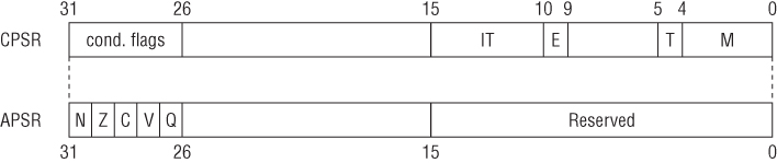
Similar to other architectures, ARM stores information about the current execution state in the current program status register (CPSR). From an application programmer's perspective, CPSR is similar to the EFLAGS/RFLAG register in x86/x64. Some documentation may discuss the application program status register (APSR), which is an alias for certain fields in the CPSR. There are many flags in the CPSR, some of which are illustrated in Figure 2.1 (others are covered in later sections).
ARM offers the concept of coprocessors to support additional instructions and system-level settings. For example, if the system supports a memory management unit (MMU), then its settings must be exposed to boot or kernel code. On x86/x64, these settings are stored in CR0 and CR4; on ARM, they are stored in coprocessor 15. There are 16 coprocessors in the ARM architecture, each identified by a number: CP0, CP1, . . . , CP15. (When used in code, these are referred to as P0, . . . , P15.) The first 13 are either optional or reserved by ARM; the optional ones can be used by manufacturers to implement manufacturer-specific instructions or features. For example, CP10 and CP11 are usually used for floating-point and NEON support. Each coprocessor contains additional “opcodes” and registers that can be controlled through special ARM instructions. CP14 and CP15 are used for debug and system settings; CP15, usually known as the system control coprocessor, stores most of the system settings (caching, paging, exceptions, and so forth).
Each coprocessor has 16 registers and eight corresponding opcodes. The semantic of these registers and opcodes is specific to the coprocessor. Accessing coprocessors can only be done through the MRC (read) and MCR (write) instructions; they take a coprocessor number, register number, and opcodes. For example, to read the translation base register (similar to CR3 in x86/x64) and save it in R0, you use the following:
MRC p15, 0, r0, c2, c0, 0 ; save TTBR in r0
This says, “read coprocessor 15's C2/C0 register using opcode 0/0 and store the result in the general-purpose register R0.” Because there are so many registers and opcodes within each coprocessor, you must read the documentation to determine the precise meaning of each. Some registers (C13/C0) are reserved for operating systems in order to store process- or thread-specific data.
While the MRC and MCR instructions do not require high privilege (i.e., they can be executed in USR mode), some of the coprocessor registers and opcodes are only accessible in SVC mode. Attempts to read certain registers without sufficient privilege will result in an exception. In practice, you will infrequently see these instructions in user-mode code; they are commonly found in very low-level code such as ROM, boot loaders, firmware, or kernel-mode code.
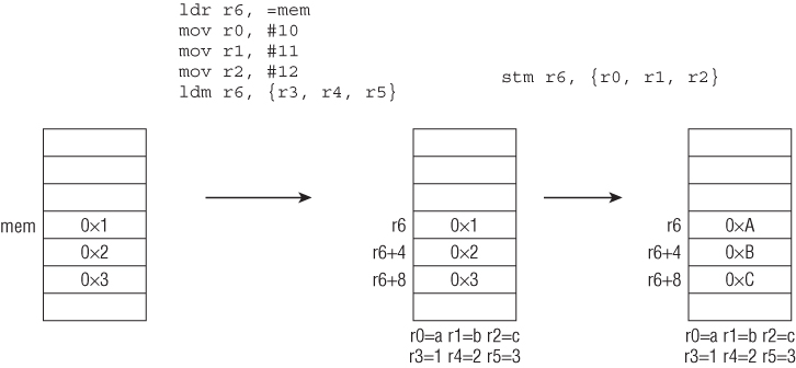
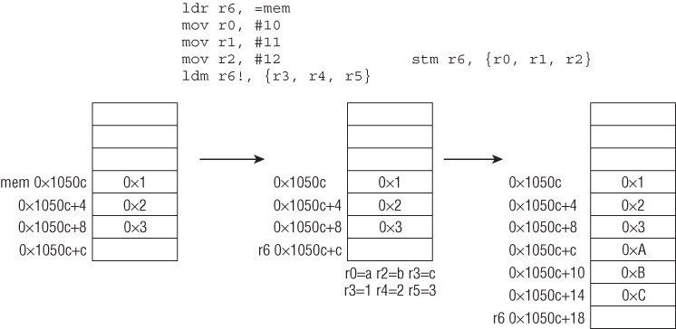
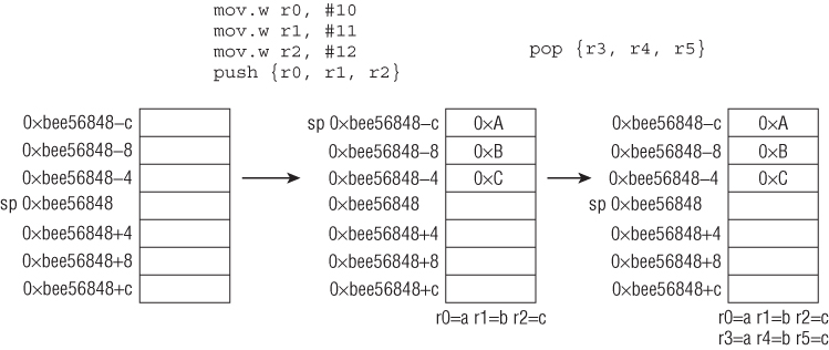
At this point, you are ready to look at the important ARM instructions. Besides conditional execution and barrel shifters, there are several other peculiarities about the instructions that are not found in x86. First, some instructions can operate on a range of registers in sequence. For example, to store five registers, R6–R10, at a particular memory location referenced by R1, you would write STM R1, {R6-R10}. R6 would be stored at memory address R1, R7 at R1+4, R8 at R1+8, and so on. Nonconsecutive registers can also be specified via comma separation (e.g., {R1,R5,R8}). In ARM assembly syntax, the register ranges are usually specified inside curly brackets. Second, some instructions can optionally update the base register after a read/write operation. This is usually done by affixing an exclamation mark (!) after the register name. For example, if you were to rewrite the previous instruction as STM R1!, {R6-R10} and execute it, then R1 will be updated with the address immediately after where R10 was stored. To make it clearer, here is an example:
01: (gdb) disas main
02: Dump of assembler code for function main:
03: => 0x00008344 <+0>:     mov     r6,  #10
04:    0x00008348 <+4>:     mov     r7,  #11
05:    0x0000834c <+8>:     mov     r8,  #12
06:    0x00008350 <+12>:    mov     r9,  #13
07:    0x00008354 <+16>:    mov     r10, #14
08:    0x00008358 <+20>:    stmia   sp!, {r6, r7, r8, r9, r10}
09:    0x0000835c <+24>:    bx      lr
10: End of assembler dump.
11: (gdb) si
12: 0x00008348 in main ()
13: …
14: 0x00008358 in main ()
15: (gdb) info reg sp
16: sp             0xbedf5848       0xbedf5848
17: (gdb) si
18: 0x0000835c in main ()
19: (gdb) info reg sp
20: sp             0xbedf585c       0xbedf585c
21: (gdb) x/6x 0xbedf5848
22: 0xbedf5848:     0x0000000a      0x0000000b      0x0000000c      0x0000000d
23: 0xbedf5858:     0x0000000e      0x00000000
Line 15 displays the value of SP (0xbedf5848) before executing the STM instruction; lines 17 and 19 execute the STM instruction and display the updated value of SP. Line 21 dumps six words starting at the old value of SP. Note that R6 was stored at the old SP, R7 at SP+0x4, R8 at SP+0x8, R9 at SP+0xc, and R10 at SP+0x10. The new SP (0xbedf585c) is immediately after where R10 was stored.
The preceding section mentions that ARM is a load-store architecture, which means that data must be loaded into registers before it can be operated on. The only instructions that can touch memory are load and store; all other instructions can operate only on registers. To load means to read data from memory and save it in a register; to store means to write the content of a register to a memory location. On ARM, the load/store instructions are LDR/STR, LDM/STM, and PUSH/POP.
These instructions can load and store 1, 2, or 4 bytes to and from memory. Their full syntax is somewhat complicated because there are several different ways to specify the offset and side effects for updating the base register. Consider the simplest case:
01: 03 68         LDR             R3, [R0] ; R3 = *R0
02: 23 60         STR             R3, [R4] ; *R4 = R3;
For the instruction in line 1, R0 is the base register and R3 is the destination; it loads the word value at address R0 into R3. In line 2, R4 is the base register and R3 is the destination; it takes the value in R3 and stores at the memory address R4. This example is simple because the memory address is specified by the base register.
At a fundamental level, the LDR/STR instructions take a base register and an offset; there are three offset forms and three addressing modes for each form. We begin by discussing the offset forms: immediate, register, and scaled register.
The first offset form uses an immediate as the offset. An immediate is simply an integer. It is added to or subtracted from the base register to access data at an offset known at compile time. The most common usage is to access a particular field in a structure or vtable. The general format is as follows:
Rb is the base register, and imm is the offset to be added to Rb.
For example, suppose that R0 holds a pointer to a KDPC structure and the following code:
Structure Definition
0:000> dt ntkrnlmp!_KDPC
   +0x000 Type             : UChar
   +0x001 Importance       : UChar
   +0x002 Number           : Uint2B
   +0x004 DpcListEntry     : _LIST_ENTRY
   +0x00c DeferredRoutine  : Ptr32     void
   +0x010 DeferredContext  : Ptr32 Void
   +0x014 SystemArgument1  : Ptr32 Void
   +0x018 SystemArgument2  : Ptr32 Void
   +0x01c DpcData          : Ptr32 Void
Code
01: 13 23         MOVS    R3, #0x13
02: 03 70         STRB    R3, [R0]
03: 01 23         MOVS    R3, #1
04: 43 70         STRB    R3, [R0,#1]
05: 00 23         MOVS    R3, #0
06: 43 80         STRH    R3, [R0,#2]
07: C3 61         STR     R3, [R0,#0x1C]
08: C1 60         STR     R1, [R0,#0xC]
09: 02 61         STR     R2, [R0,#0x10]
In this case, R0 is the base register and the immediates are 0x1, 0x2, 0xC, 0x10, and 0x1C. The snippet can be translated into C as follows:
KDPC *obj = …;             /* R0 is obj */
obj->Type = 0x13;
obj->Importance = 0x1;
obj->Number = 0x0;
obj->DpcData = NULL;
obj->DeferredRoutine = R1;   /* R1 is unknown to us */
obj->DeferredContext = R2;   /* R2 is unknown to us */
This offset form is similar to the MOV Reg, [Reg + Imm] on the x86/x64.
The second offset form uses a register as the offset. It is commonly used in code that needs to access an array but the index is computed at runtime. The general format is as follows:
Depending on the context, either Rb or Rc can be the base/offset. Consider the following two examples:
Example 1
01: 03 F0 F2 FA   BL  strlen
02: 06 46         MOV R6, R0
; R0 is strlen's return value
03: …
04: BB 57         LDRSB R3, [R7,R6]
; in this case, R6 is the offset
Example 2
01: B3 EB 05 08   SUBS.W  R8, R3, R5
02: 2F 78         LDRB    R7, [R5]
03: 18 F8 05 30   LDRB.W  R3, [R8,R5]
; here, R5 is the base and R8 is the offset
04: 9F 42         CMP     R7, R3
This is similar to the MOV Reg, [Reg + Reg] form on x86/x64.
The third offset form uses a scaled register as the offset. It is commonly used in a loop to iterate over an array. The barrel shifter is used to scale the offset. The general format is as follows:
Rb is the base register; Rc is an immediate; and <shifter> is the operation performed on the immediate—typically, a left/right shift to scale the immediate. For example:
01: 0E 4B         LDR     R3, =KeNumberNodes
02: …
03: 00 24         MOVS    R4, #0
04: 19 88         LDRH    R1, [R3]
05: 09 48         LDR     R0, =KeNodeBlock
06: 00 23         MOVS    R3, #0
07:             loop_start
08: 50 F8 23 20   LDR.W   R2, [R0,R3,LSL#2]
09: 00 23         MOVS    R3, #0
10: A2 F8 90 30   STRH.W  R3, [R2,#0x90]
11: 92 F8 89 30   LDRB.W  R3, [R2,#0x89]
12: 53 F0 02 03   ORRS.W  R3, R3, #2
13: 82 F8 89 30   STRB.W  R3, [R2,#0x89]
14: 63 1C         ADDS    R3, R4, #1
15: 9C B2         UXTH    R4, R3
16: 23 46         MOV     R3, R4
17: 8C 42         CMP     R4, R1
18: EF DB         BLT     loop_start
KeNumberNodes and KeNodeBlock are a global integer and an array of KNODE pointers, respectively.
Lines 1 and 5 simply load those globals into a register (we explain this syntax later). Line 8 iterates over the KeNodeBlock array (R0 is the base), R3 is the index multiplied by 2 (because it is an array of pointers; pointers are 4 bytes in size on this platform). Lines 10–13 initialize some fields of the KNODE element. Line 14 increments the index. Line 17 compares the index against the size of the array (R1 is the size; see line 4) and if it is less than the size then continues the loop.
This snippet can be roughly translated to C as follows:
int KeNumberNodes = …;
KNODE *KeNodeBlock[KeNumberNodes] = …;
for (int i=0; i < KeNumberNodes; i++) {
    KeNodeBlock[i].x = …;
    KeNodeBlock[i].y = …;
    …
}
This is similar to the MOV, Reg, [Reg + idx * scale] form on x86/x64.
Having covered the three offset forms, the rest of this section discusses addressing modes: offset, pre-indexed, and post-indexed. The only distinction among them is whether the base register is modified and, if so, in what way. All the preceding offset examples use offset addressing mode, which means that the base register is never modified. This is the simplest and most common mode. You can quickly recognize it because it does not contain an exclamation mark (!) anywhere and the immediate is inside the square brackets. (Some publications categorize these modes as pre-index, pre-index with writeback, and post-index. The terminology used here reflects the official ARM documentation.) The general syntax for the offset mode is LDR Rd, [Rn, offset].
Pre-indexed address mode means that the base register will be updated with the final memory address used in the reference operation. The semantic is very similar to the prefix form of the unary ++ and -- operator in C. The syntax for this mode is LDR Rd, [Rn, offset]!. For example:
12 F9 01 3D   LDRSB.W R3, [R2 ,#-1]! ; R3 = *(R2-1)
                                     ; R2 = R2-1
Post-indexed address mode means that the base register is used as the final address, then updated with the offset calculated. This is very similar to the postfix form of the unary ++ and -- operator in C. The syntax for this mode is LDR Rd, [Rn], offset. For example:
10 F9 01 6B   LDRSB.W R6, [R0],#1  ; R6 = *R0
                                   ; R0 = R0+1
The pre- and post-index forms are normally observed in code that accesses an offset in the same buffer multiple times. For example, suppose the code needs to loop and check whether a character in a string matches one of five characters; the compiler may update the base pointer so that it can shave off an increment instruction.
As explained earlier, LDR is used to load data from memory into a register; however, sometimes you see it in these forms:
01: DF F8 50 82   LDR.W   R8, =0x2932E00 ; LDR R8, [PC, x]
02: 80 4A         LDR     R2, =a04d ; "%04d" ; LDR R2, [PC, y]
03: 0E 4B         LDR     R3, =__imp_realloc ; LDR R3, [PC, z]
Clearly, this is not valid syntax according to the previous section. Technically, these are called pseudo-instructions and they are used by disassemblers to make manual inspection easier. Internally, they use the immediate form of LDR with PC as a base register; sometimes, this is called PC-relative addressing (or RIP-relative addressing on x64). ARM binaries usually have a literal pool that is a memory area in a section to store constants, strings, or offsets that others can reference in a position-independent manner. (The literal pool is part of the code, so it will be in the same section.) In the preceding snippet, the code is referencing a 32-bit constant, a string, and an offset to an imported function stored in the literal pool. This particular pseudo-instruction is useful because it allows a 32-bit constant to be moved into a register in one instruction. To make it clearer, consider the following snippet:
01: .text:0100B134 35 4B   LDR    R3, =0x68DB8BAD
                ; actually LDR R3, [PC, #0xD4]
                ; at this point, PC = 0x0100B138
02: …
03: .text:0100B20C AD 8B DB 68 dword_100B20C DCD 0x68DB8BAD
How did the disassembler shorten the first instruction from LDR R3, [PC, #0xD4] to the alternate form? Because the code is in Thumb state, PC is the current instruction plus 4, which is 0x0100B138; it is using the immediate form of PC, so it is trying to read the word at 0x0100B20C (=0x100B138+0xD4), which happens to be the constant we want to load.
Another related instruction is ADR, which gets the address for a label/function and puts it in a register. For example:
01: 00009390 65 A5         ADR     R5, dword_9528
02: 00009392 D5 E9 00 45   LDRD.W  R4, R5, [R5]
03: …
04: 00009528 00 CE 22 A9+dword_9528 DCD 0xA922CE00 , 0xC0A4
This instruction is typically used to implement jump tables or callbacks where you need to pass the address of a function to another. Internally, this instruction just calculates an offset from PC and saves it in the destination register.
LDM and STM are similar to LDR/STR except that they load and store multiple words at a given base register. They are useful when moving multiple data blocks to and from memory. The general syntax is as follows:
Rn is the base register and it holds the memory address to load/store from; the optional exclamation mark (!) means that the base register should be updated with the new address (writeback). Rm is the range of register to load/store. There are four modes:
This may sound a bit confusing at first, so let's walk through an example with the debugger:
01: (gdb) br main
02: Breakpoint 1 at 0x8344
03: (gdb) disas main
04: Dump of assembler code for function main:
05:    0x00008344 <+0>:     ldr     r6, =mem  ; edited a bit
06:    0x00008348 <+4>:     mov     r0, #10
07:    0x0000834c <+8>:     mov     r1, #11
08:    0x00008350 <+12>:    mov     r2, #12
09:    0x00008354 <+16>:    ldm     r6, {r3, r4, r5}  ; IA mode
10:    0x00008358 <+20>:    stm     r6, {r0, r1, r2}  ; IA mode
11: …
12: (gdb) r
13: Breakpoint 1, 0x00008344 in main ()
14: (gdb) si
15: 0x00008348 in main ()
16: (gdb) x/3x $r6
17: 0x1050c <mem>:  0x00000001      0x00000002      0x00000003
18: (gdb) si
19: 0x0000834c in main ()
20: …
21: (gdb)
22: 0x00008358 in main ()
23: (gdb) info reg r3 r4 r5
24: r3             0x1      1
25: r4             0x2      2
26: r5             0x3      3
27: (gdb) si
28: 0x0000835c in main ()
29: (gdb) x/3x $r6
30: 0x1050c <mem>:  0x0000000a      0x0000000b      0x0000000c
Line 5 stores a memory address in R6; the content of this memory address (0x1050c) is three words (line 17). Lines 6–8 set R0–R2 with some constants. Line 9 loads three words into R3–R5, starting at the memory location specified by R6. As shown in lines 24–26, R3–R5 contain the expected value. Line 10 stores R0–R2, starting at the memory location specified by R6. Line 29 shows that the expected values were written. Figure 2.2 illustrates the result of the preceding operations.
Here's the same experiment with writeback:
01: (gdb) br main
02: Breakpoint 1 at 0x8344
03: (gdb) disas main
04: Dump of assembler code for function main:
05:    0x00008344 <+0>:     ldr     r6, =mem   ; edited a bit
06:    0x00008348 <+4>:     mov     r0, #10
07:    0x0000834c <+8>:     mov     r1, #11
08:    0x00008350 <+12>:    mov     r2, #12
09:    0x00008354 <+16>:    ldm     r6!, {r3, r4, r5} ; IA mode w/ writeback
10:    0x00008358 <+20>:    stmia   r6!, {r0, r1, r2} ; IA mode w/ writeback
11: …
12: (gdb) r
13: Breakpoint 1, 0x00008344 in main ()
14: (gdb) si
15: 0x00008348 in main ()
16: …
17: (gdb)
18: 0x00008354 in main ()
19: (gdb) x/3x $r6
20: 0x1050c <mem>:  0x00000001      0x00000002      0x00000003
21: (gdb) si
22: 0x00008358 in main ()
23: (gdb) info reg r6
24: r6             0x10518  66840
25: (gdb) si
26: 0x0000835c in main ()
27: (gdb) info reg $r6
28: r6             0x10524  66852
29: (gdb) x/4x $r6-12
30: 0x10518 :       0x0000000a      0x0000000b      0x0000000c      0x00000000
Line 9 uses IA mode with writeback, so the r6 is updated with an address 4 bytes above the last location (line 23). The same can be observed in lines 10, 27, and 30. Figure 2.3 shows the result of the preceding snippet.
Because LDM and STM can move multiple words at a time, they are typically used in block- copy or move operations. For example, they are sometimes used to inline memcpy when the copy length is known at compile time. They are similar to the MOVS instruction with the REP prefix on x86. Consider the following blobs of code generated by two different compilers from the same source file:
Compiler A
01: A4 46         MOV      R12, R4
02: 35 46         MOV      R5, R6
03: BC E8 0F 00   LDMIA.W  R12!, {R0-R3}
04: 0F C5         STMIA    R5!, {R0-R3}
05: BC E8 0F 00   LDMIA.W  R12!, {R0-R3}
06: 0F C5         STMIA    R5!, {R0-R3}
07: 9C E8 0F 00   LDMIA.W  R12, {R0-R3}
08: 85 E8 0F 00   STMIA.W  R5, {R0-R3}
Compiler B
01: 30 22         MOVS   R2, #0x30
02: 21 46         MOV    R1, R4
03: 30 46         MOV    R0, R6
04: 23 F0 17 FA   BL     memcpy
All this does is copy 48 bytes from one buffer to another; the first compiler uses LDM/STM with writebacks to load/store 16 bytes at a time, while the second simply calls into its implementation of memcpy. When reverse engineering code, you can spot the inlined memcpy form by recognizing that the same source and destination pointers are being used by LDM/STM with the same register set. This is a good trick to keep in mind because you will see it often.
Another common place where LDM/STM can be seen is at the beginning and end of functions in ARM state. In this context, they are used as the prologue and epilogue. For example:
01: F0 4F 2D E9   STMFD   SP!, {R4-R11,LR}  ; save regs + return address
02: …
03: F0 8F BD E8   LDMFD   SP!, {R4-R11,PC}  ; restore regs and return
STMFD and LDMFD are pseudo-instructions for STMDB and LMDIA/LDM, respectively.
The final set of load/store instructions is PUSH and POP. They are similar to LDM/STM except for two characteristics:
The stack grows downward to lower addresses as it does in the x86/x64 architecture. The general syntax is PUSH/POP {Rn}, where Rn can be a range of registers.
PUSH stores the registers on the stack such that the last location is 4 bytes below the current stack pointer, and updates SP with the address of the first location. POP loads the registers starting from the current stack pointer and updates SP with the address 4 bytes above the last location. PUSH/POP are actually the same as STMDB/LDMIA with writeback and SP as the base pointer. Here is a short walk-through demonstrating the instructions:
01: (gdb) disas main
02: Dump of assembler code for function main:
03:    0x00008344 <+0>:     mov.w   r0, #10
04:    0x00008348 <+4>:     mov.w   r1, #11
05:    0x0000834c <+8>:     mov.w   r2, #12
06:    0x00008350 <+12>:    push    {r0, r1, r2}
07:    0x00008352 <+14>:    pop     {r3, r4, r5}
08: …
09: (gdb) br main
10: Breakpoint 1 at 0x8344
11: (gdb) r
12: Breakpoint 1, 0x00008344 in main ()
13: (gdb) si
14: 0x00008348 in main ()
15: …
16: (gdb)
17: 0x00008350 in main ()
18: (gdb) info reg sp        ; current stack pointer
19: sp             0xbee56848       0xbee56848
20: (gdb) si
21: 0x00008352 in main ()
22: (gdb) x/3x $sp           ; sp is updated after the push
23: 0xbee5683c:     0x0000000a      0x0000000b      0x0000000c
24: (gdb) si                 ; pop into the registers
25: 0x00008354 in main ()
26: (gdb) info reg r3 r4 r5  ; new registers
27: r3             0xa      10
28: r4             0xb      11
29: r5             0xc      12
30: (gdb) info reg sp        ; new sp (4 bytes above the last location)
31: sp             0xbee56848       0xbee56848
32: (gdb) x/3x $sp-12
33: 0xbee5683c:     0x0000000a      0x0000000b      0x0000000c
Figure 2.4 illustrates the preceding snippet.
The most common place for PUSH/POP is at the beginning and end of functions. In this context, they are used as the prologue and epilogue (like STMFD/LDMFD in ARM state). For example:
01: 2D E9 F0 4F   PUSH.W  {R4-R11,LR} ; save registers + return address
02: …
03: BD E8 F0 8F   POP.W   {R4-R11,PC} ; restore registers and return
Some disassemblers actually use this pattern as a heuristic to determine function boundaries.
Unlike x86/x64, which has only one instruction for function invocation (CALL) and branching (JMP), ARM offers several depending on how the destination is encoded. When you call a function, the processor needs to know where to resume execution after the function returns; this location is typically referred to as the return address. In x86, the CALL instruction implicitly pushes the return address on the stack before jumping to the target function; when it is done executing, the target function resumes execution at the return address by popping it off the stack into EIP.
The mechanism on ARM is essentially the same with a few minor differences. First, the return address can be stored on the stack or in the link register (LR); to resume execution after the call, the return address is explicitly popped off the stack into PC or there will be an unconditional branch to LR. Second, a branch can switch between ARM and Thumb state, depending on the destination address's LSB. Third, a standard calling convention is defined by ARM: The first four 32-bit parameters are passed via registers (R0-R3) and the rest are on the stack. Return value is stored in R0.
The instructions used for function invocations are B, BX, BL, and BLX.
Although it is rare to see B used in the context of function invocation, it can be used for transfer of control. It is simply an unconditional branch and is identical to the JMP instruction in x86. It is normally used inside of loops and conditionals to go back to the beginning or break out; it can also be used to call a function that never returns. B can only use label offsets as its destination; it cannot use registers. In this context, the syntax of B is as follows: B imm, where imm is an offset relative from the current instruction. (This does not take into consideration the conditional execution flags, which are discussed in the “Branching and Conditional Execution” section.) One important fact to note is that because ARM and Thumb instructions are 4- and 2-byte aligned, the target offset needs to be an even number. Here is a snippet showing the usage of B:
01: 0001C788   B         loc_1C7A8
02: 0001C78A
03: 0001C78A loc_1C78A
04: 0001C78A   LDRB      R7, [R6,R2]
05: …
06: 0001C7A4   STRB.W    R7, [R3,#-1]
07: 0001C7A8
08: 0001C7A8 loc_1C7A8
09: 0001C7A8   MOV       R7, R3
10: 0001C7AA   ADDS      R3, #2
11: 0001C7AC   CMP       R2, R4
12: 0001C7AE   BLT       loc_1C78A
In line 1, you see B being used as an unconditional jump to start off a loop. You can ignore the other instructions for now.
BX is Branch and Exchange. It is similar to B in that it transfers control to a target, but it has the ability to switch between ARM/Thumb state, and the target address is stored in a register. Branching instructions that end with X indicate that they are capable of switching between states. If the LSB of the target address is 1, then the processor automatically switches to Thumb state; otherwise, it executes in ARM state. The instruction format is BX <register>, where register holds the destination address. The two most common uses of this instruction are returning from a function by branching to LR (i.e., BX LR) and transferring of control to code in a different mode (i.e., going from ARM to Thumb or vice versa). In compiled code, you will almost always see BX LR at the end of functions; it is basically the same as RET in x86.
BL is Branch with Link. It is similar to B except that it also stores the return address in LR before transferring control to the target offset. This is probably the closest equivalence to the CALL instruction in x86 and you will often see it used to invoke functions. The instruction format is the same as B (that is, it takes only offsets). Here is a short snippet demonstrating function invocation and returning:
01: 00014350   BL              foo ; LR = 0x00014354
02: 00014354   MOVS            R4, #0x15
03: …
04: 0001B224 foo
05: 0001B224   PUSH            {R1-R3}
06: 0001B226   MOV             R3, 0x61240
07: …
08: 0001B24C   BX              LR  ; return to 0x00014354
Line 1 calls the function foo using BL; before transferring control to the destination, BL stores the return address (0x000014354) in LR. foo does some work and returns to the caller (BX LR).
BLX is Branch with Link and Exchange. It is like BL with the option to switch state. The major difference is that BLX can take either a register or an offset as its branch destination; in the case where BLX uses an offset, the processor always swaps state (ARM to Thumb and vice versa). Because it shares the same characteristics as BL, you can also think of it as the equivalent of the CALL instruction in x86. In practice, both BL and BLX are used to call functions. BL is typically used if the function is within a 32MB range, and BLX is used whenever the target range is undetermined (like a function pointer). When operating in Thumb state, BLX is usually used to call library routines; in ARM state, BL is used instead.
Having explored all instructions related to unconditional branching and direct function invocation, and how to return from a function (BX LR), you can consolidate your knowledge by looking at a full routine:
01: 0100C388             ; void *__cdecl mystery(int)
02: 0100C388             mystery
03: 0100C388 2D E9 30 48   PUSH.W  {R4,R5,R11,LR}
04: 0100C38C 0D F2 08 0B   ADDW    R11, SP, #8
05: 0100C390 0C 4B         LDR     R3, =__imp_malloc
06: 0100C392 C5 1D         ADDS    R5, R0, #7
07: 0100C394 6F F3 02 05   BFC.W   R5, #0, #3
08: 0100C398 1B 68         LDR     R3, [R3]
09: 0100C39A 15 F1 08 00   ADDS.W  R0, R5, #8
10: 0100C39E 98 47         BLX     R3
11: 0100C3A0 04 46         MOV     R4, R0
12: 0100C3A2 24 B1         CBZ     R4, loc_100C3AE
13: 0100C3A4 EB 17         ASRS    R3, R5, #0x1F
14: 0100C3A6 63 60         STR     R3, [R4,#4]
15: 0100C3A8 25 60         STR     R5, [R4]
16: 0100C3AA 08 34         ADDS    R4, #8
17: 0100C3AC 04 E0         B       loc_100C3B8
18: 0100C3AE             loc_100C3AE
19: 0100C3AE 04 49         LDR     R1, =aFailed ; "failed…"
20: 0100C3B0 2A 46         MOV     R2, R5
21: 0100C3B2 07 20         MOVS    R0, #7
22: 0100C3B4 01 F0 14 FC   BL      foo
23: 0100C3B8
24: 0100C3B8             loc_100C3B8
25: 0100C3B8 20 46         MOV     R0, R4
26: 0100C3BA BD E8 30 88   POP.W   {R4,R5,R11,PC}
27: 0100C3BA             ; End of function mystery
This function covers several of the ideas discussed earlier (ignore the other instructions for now):
After loading a value from memory into a register, the code can move it around and perform operations on it. The simplest operation is to move it to another register with the MOV instruction. The source can be a constant, a register, or something processed by the barrel shifter. Here are examples of its usage:
01: 4F F0 0A 00   MOV.W   R0, #0xA  ; r0 = 0xa
02: 38 46         MOV     R0, R7    ; r0 = r7
03: A4 4A A0 E1   MOV     R4, R4, LSR #21 ; r4 = (r421)
Line 3 shows the source operand being processed by the barrel shifter before being moved to the destination. The barrel shifter's operations include left shift (LSL), right shift (LSR, ASR), and rotate (ROR, RRX). The barrel shifter is useful because it allows the instruction to work on constants that cannot normally be encoded in immediate form. ARM and Thumb instructions can be either 16 or 32 bits wide, so they cannot directly have 32-bit constants as a parameter; with the barrel shifter, an immediate can be transformed into a larger value and moved to another register. Another way to move a 32-bit constant into a register is to split the constant into two 16-bit halves and move them one a time; this is normally done with the MOVW and MOVT instructions. MOVT sets the top 16 bits of a register, and MOVW sets the bottom 16 bits.
The basic arithmetic and logical operations are ADD, SUB, MUL, AND, ORR, and EOR. Here are examples of their usage:
01: 4B 44 ADD R3, R9 ; r3 = r3+r9 02: 0D F2 08 0B ADDW R11, SP, #8 ; r11 = sp+8 03: 04 EB 80 00 ADD.W R0, R4, R0,LSL#2 ; r0 = r4 + (r0
Note the “S” after some of these instructions. Unlike x86, ARM arithmetic instructions do not set the conditional flag by default. The “S” suffix indicates that the instruction should set arithmetic conditional flags (zero, negative, etc.) depending on its result. Note that the MUL instruction truncates the result such that only the bottom 32 bits are stored in the destination register; for full 64-bit multiplication, use the SMULL and UMULL instructions (see ARM TRM for the details).
Where is the divide instruction? ARM does not have a native divide instruction. (ARMv7-R and ARMv7-M cores have SDIV and UDIV, but they are not discussed here.) In practice, the runtime will have a software implementation for division and code simply call into it when needed. Here is an example with the Windows C runtime:
01: 41 46         MOV             R1, R8
02: 30 46         MOV             R0, R6
03: 35 F0 9E FF   BL              __rt_udiv ; software implementation of udiv
Every example discussed so far has been executed in a linear manner. Most programs will have conditionals and loops. At the assembly level, these constructs are implemented using conditional flags, which are stored in the application program status register (APSR). The APSR is an alias of the CPSR and is similar to the EFLAG in x86. Figure 2.5 illustrates the relevant flags, described as follows:
The N, Z, C, and V bits are identical to the SF, ZF, CF, and OF bits in the EFLAG register on x86. They are used to implement conditionals and loops in higher-level languages; they are also used to support conditional execution at the instruction level. Equality is described in terms of these flags. Table 2.1 shows common relationships and corresponding flags.
Table 2.1 Conditional code and meaning
| Suffix/Code | Meaning | Flags |
| EQ | Equal | Z==1 |
| NE | Not equal | Z==0 |
| MI | Minus, negative | N==1 |
| PL | Plus, positive, or zero | N==0 |
| HI | Unsigned higher/above | C==1 and Z==0 |
| LS | Unsigned lower/below | C==0 or Z==1 |
| GE | Signed greater than or equal | N==V |
| LT | Signed less than | N!=V |
| GT | Signed greater than | Z==0 and N==V |
| LE | Signed less than or equal | Z==1 or N!=V |
Instructions can be conditionally executed by adding one of these suffixes at the end. For example, BLT means to branch if the LT condition is true. (This is the same as JL in x86.) By default, instructions do not update conditional flags unless the “S” suffix is used; the comparison instructions (CBZ, CMP, TST, CMN, and TEQ) update the flags automatically because they are usually used before branch instructions.
The most common comparison instruction is probably CMP. Its syntax is CMP Rn, X, where Rn is a register and X can be an immediate, a register, or a barrel shift operation. Its semantic is identical to that in x86: It performs Rn - X, sets the appropriate flags, and discards the result. It is usually followed by a conditional branch. Here is an example of its usage and pseudo-code:
ARM
01: B3 EB E7 7F   CMP.W     R3, R7, ASR #31
02: 05 DB         BLT       loc_less
03: 01 DC         BGT       loc_greater
04: BD 42         CMP       R5, R7
05: 02 D9         BLS       loc_less
06:             loc_greater
07: 07 3D         SUBS      R5, #7
08: 6E F1 00 0E   SBC.W     LR, LR, #0
09:             loc_less
10: A5 FB 08 12   UMULL.W   R1, R2, R5, R8
11: 87 FB 08 04   SMULL.W   R0, R4, R7, R8
12: 0E FB 08 23   MLA.W     R3, LR, R8, R2
Pseudo C
if (r3 < r7) { goto loc_less; }
else if ( r3 > r7) { goto loc_greater; }
else if ( r5 < r7) { goto loc_less; }
The next most common comparison instruction is TST; its syntax is identical to that of CMP. Its semantic is identical to TEST in x86: It performs Rn & X, sets the appropriate flags, and discards the result. It is usually used to test whether a value is equal to another or to test for flags. Like most compare instructions, it is typically followed by a conditional branch. Here is an example:
01: AB 8A         LDRH     R3, [R5,#0x14]
02: 13 F0 02 0F   TST.W    R3, #2
03: 09 D0         BEQ      loc_10179DA
04: …
05:             loc_10179BE
06: AA 8A         LDRH     R2, [R5,#0x14]
07: 12 F0 04 0F   TST.W    R2, #4
08: 02 D0         BEQ      loc_10179E8
In Thumb-2 state, there are two popular comparison instructions: CBZ and CBNZ. Their syntax is simple: CBZ/CBNZ Rn, label, where Rn is a register and label is an offset to branch to if the condition is true. CBZ then branches to label if the register is zero. CBNZ is same except that it checks for a non-zero condition. These instructions are usually used to determine whether a number is 0 or a pointer is NULL. Here is a typical usage:
ARM
01: 10 F0 48 FF   BL          foo
             ; foo returns a pointer in r0
02: 28 B1         CBZ         R0, loc_100BC8E
03: …
04:             loc_100BC8E
05: 01 20         MOVS        R0, #1
06: 28 E0         B           locret_100BCE4
07: …
08:             locret_100BCE4
09: BD E8 F8 89   POP.W       {R3-R8,R11,PC}
Pseudo C
type *a;
a = foo(…);
if (a == NULL) { return 1; }
The other comparison instructions are CMN/TEQ, which performs addition/exclusive-or on the operands. Because they are not commonly used they are not covered here.
You have seen that the branch instruction (B) can be made to do conditional branches by adding a suffix (BEQ, BLE, BLT, BLS, etc.). In fact, most ARM instructions can be conditionally executed in the same way. If the condition is not met, the instruction can be seen as a no-op. Instruction-level conditional execution can reduce branches, which may speed up execution time. Here is an example:
ARM
01: 00 00 50 E3   CMP     R0, #0
02: 01 00 A0 03   MOVEQ   R0, #1
03: 68 00 D0 15   LDRNEB  R0, [R0,#0x68]
04: 1E FF 2F E1   BX      LR
Pseudo C
unk_type *a = …;
if (a == NULL) { return 1; }
else { return a->off_48; }
You immediately know that R0 is a pointer because of the LDR instruction in line 3. Line 1 checks whether R0 is NULL. If true (EQ), then line 2 sets R0 to 1; otherwise, NEQ loads the value at R0+0x68 into R0 (line 3) and then returns. Because EQ and NEQ cannot be true at the same time, only one of the instructions will be executed. Note that there are no branch instructions.
Unlike most ARM instructions, Thumb instructions cannot be conditionally executed (with the exception of B) without the IT (if-then) instruction. This is a Thumb-2-specific instruction that allows up to four instructions after it to be conditionally executed. The general syntax is as follows: ITxyz cc, where cc is the conditional code for the first instruction; x, y, and z describe the condition for the second, third, and fourth instruction, respectively. Conditions for instructions after the first are described by one of two letters: T or E. T means that the condition must match cc to be executed; E means to execute only if the condition is the inverse of cc. Consider the following example:
ARM
01: 00 2B         CMP     R3, #0
           ; check and set condition
02: 12 BF         ITEE NE
           ; begin IT block
03: BC FA 8C F0   CLZNE.W R0, R12
           ; first instruction
04: B6 FA 86 F0   CLZEQ.W R0, R6
           ; second instruction
05: 20 30         ADDEQ   R0, #0x20
           ; third instruction
Pseudo C
if (R3 != 0) {
 R0 = countleadzeros(R12);
} else {
 R0 = countleadzeros(R6);
 R0 += 0x20
}
Line 1 performs a comparison and sets a conditional flag. Line 2 specifies the conditions and start the if-then block. NE is the execution condition for the first instruction; the first E (after IT) indicates that the execution condition for the second instruction is the inverse of the first. (EQ is the inverse of NE.) The second E indicates the same for the third instruction. Lines 3–5 are instructions inside the IT block.
Due to its flexibility, the IT instruction can be used to reduce the number of instructions required to implement short conditionals in Thumb state.
Switch-case statements can be understood as many if-else statements bundled together. Because the test expression and target label are known at compile time, compilers usually construct a jump table to store addresses (ARM) or offsets (Thumb) for each case handler. After determining the index into the jump table, the compiler indirectly branches to the destination by loading the destination address into PC. In ARM state, this is normally done by LDR with PC as the destination and base register. Consider the following example:
01:  ; R1 is the case
02: 0B 00 51 E3   CMP      R1, #0xB   ; is it within range?
03: 01 F1 9F 97   LDRLS    PC, [PC,R1,LSL#2] ; yes, switch by
                                      ; indexing into the table
04: 14 00 00 EA   B        loc_DD10  ; no, break
05: 3C DD 00 00+  DCD loc_DD3C  ; begin of jump table
06: 4C DD 00 00+  DCD loc_DD4C
07: 68 DD 00 00+  DCD loc_DD68
08: 8C DD 00 00+  DCD loc_DD8C
09: BC DD 00 00+  DCD loc_DDBC
10: F0 DD 00 00+  DCD loc_DDF0
11: 38 DE 00 00+  DCD loc_DE38
12: 38 DE 00 00+  DCD loc_DE38
13: EC DC 00 00+  DCD loc_DCEC  ; case/index 8
14: EC DC 00 00+  DCD loc_DCEC  ; case/index 9
15: 3C DD 00 00+  DCD loc_DD3C
16: 3C DD 00 00   DCD loc_DD3C
17:             loc_DCEC   ; handler for case 8,9
18: 00 00 A0 E3   MOV      R0, #0
19: 08 10 41 E2   SUB      R1, R1, #8
20: 04 30 A0 E3   MOV      R3, #4
21: 14 00 82 E5   STR      R0, [R2,#0x14]
22: BC 31 C2 E1   STRH     R3, [R2,#0x1C]
23: 10 10 82 E5   STR      R1, [R2,#0x10]
Line 2 checks whether the case is within range; if not, then it executes the default handler (line 4). Line 3 conditionally executes if R1 is within range; it branches to the case-handler by indexing into the jump table and loads the destination address in PC. Recall that PC is 8 bytes after the current instruction (in ARM state), so the jump table is usually stored 8 bytes from the LDR instruction.
In Thumb mode, the same concept applies except that the jump table contains offsets instead of addresses. ARM added new instructions to support table-branching with byte or half-word offsets: TBB and TBH. For TBB, the table entries are byte values; for TBH, they are half-words. The table entries must be multiplied by two and added to PC to get the final branch destination. Here is the preceding example using TBB:
01: 0101E600 0B 29         CMP     R1, #0xB ; is it within range?
02: 0101E602 76 D8         BHI     loc_101E6F2 ; no, break
03: 0101E604 04 26         MOVS    R6, #4
04: 0101E606 DF E8 01 F0   TBB.W   [PC,R1] ; branch using table offset
05: 0101E60A 06          jpt_101E606 DCB 6 ; begin of jump table
06: 0101E60B 09            DCB 9
07: 0101E60C 0F            DCB 0xF
08: 0101E60D 18            DCB 0x18
09: 0101E60E 24            DCB 0x24
10: 0101E60F 32            DCB 0x32
11: 0101E610 45            DCB 0x45
12: 0101E611 45            DCB 0x45
13: 0101E612 6D            DCB 0x6D ; offset for 8
14: 0101E613 6D            DCB 0x6D ; offset for 9
15: 0101E614 06            DCB 6
16: 0101E615 06            DCB 6
17: …
18: 0101E6E4             loc_101E6E4   ; handler for case 8,9
19: 0101E6E4 B1 F1 08 03   SUBS.W  R3, R1, #8
20: 0101E6E8 00 20         MOVS    R0, #0
21: 0101E6EA 60 61         STR     R0, [R4,#0x14]
Because it is in Thumb state, PC is 4 bytes after the current instruction; hence, for case 8, the table entry would be at address 0x0101E612 (=0x0101E60A+8), which is 0x6d, and the handler is at 0x101E6E4 (=PC+(0x6d*2)). Similar to the previous example, the jump table is usually placed after the TBB/TBH instruction. Note that the TBB/TBH are used only in Thumb state.
This section briefly discusses concepts that are not directly related to the process of reverse engineering. However, in practice, they are important to know because they may contribute to your overall knowledge. More knowledge is always good. You can skip this section on a first read.
ARM supports the concept of just-in-time (JIT) and self-modifying code (SMC). JIT code is native code that is dynamically generated by a JIT compiler; for example, the Microsoft .NET languages compile to an intermediate language (MSIL) that is converted into native machine code (x86, x64, ARM, etc.) for execution on the CPU core. SMC is code that is generated or modified by the current instruction stream. A common example of SMC is encoded shellcode that is decoded and executed at run-time. Both JIT and SMC code require writing to memory new data that is then later fetched by execution.
The ARM core has two separate cache lines for instruction (i-cache) and data (d-cache); instructions are executed from the i-cache, and memory access is through the d-cache. These cache lines are not guaranteed to be coherent, which means that data written to one cache may not be immediately visible to the other. For example, suppose the i-cache holds four instructions from the instruction stream and the user generates new or modified instructions at the same spot (which updates the d-cache). Because they are not coherent, the i-cache may not know about the recent modification, so it executes stale instructions (which may lead to mysterious crashes or incorrect results). If you are writing JIT systems or shellcode, this is clearly not a desirable situation. The solution is to explicitly force the i-cache to be refreshed (also known as flushing the cache). On ARM, this is done by updating a register in the system control coprocessor (CP15):
01: 4F F0 00 00   MOV.W     R0, #0
02: 07 EE 15 0F   MCR       p15, 0, R0,c7,c5, 0
Most operating systems provide an interface for this operation, so you do not have to write it yourself. On Linux, use __clear_cache; on Windows, use FlushInstructionCache.
ARM does not have an instruction similar to cmpxchg (compare-and-exchange) in x86; instead, two instructions are used: LDREX and STREX. These instructions are just like LDR/STR, except that they acquire exclusive access to the memory address before loading/storing. Together, they are typically used to implement compare-and-exchange intrinsics. For example:
ARM
01: 01 21         MOVS      R1, #1
02:             loc_100C4B0
03: 54 E8 00 2F   LDREX.W   R2, [R4]
04: 1A B9         CBNZ      R2, loc_100C4BE
05: 44 E8 00 13   STREX.W   R3, R1, [R4] ; r3 is the result
06: 00 2B         CMP       R3, #0
07: F8 D1         BNE       loc_100C4B0
Pseudo C
if (InterlockedCompareExchange(&r4, 1, 0) == 0) { do stuff; }
Line 3 performs an atomic load into R2 and compares it against 0; if it is zero, then it is exchanged with zero and the result is returned in R3. This is actually the implementation of InterlockedCompareExchange in Windows.
From time to time, you will run into code using the DMB, DSB, and ISB instructions. These are barrier instructions that ensure that memory access and instruction fetches are synchronized before executing subsequent instructions. This is necessary in some cases because memory access and instructions can be executed out of order (i.e., the CPU might execute the instructions in a different order than what appears in the assembly code), and other executing threads may not see the updated result and consequently have an inconsistent view of the data. For this reason, you will often see these instructions used in code that implements locks.
When an ARM core boots up, it starts executing code in the ARM state at the memory address 0x00000000 or 0xFFFF0000, depending on a setting in coprocessor 15. This is determined by the vector (V) bit in the system control register (CP15, C1/C0). If it is 0, then the exception vector is at 0x00000000; otherwise, it is at 0xFFFF0000. This address is usually in flash memory (RAM has not been initialized yet so it cannot be used), and the content therein is commonly known as the exception vectors. ARM has a list of predefined vectors starting at the base address. The RESET exception handler is first in the table so it is executed after a reset event. Because it is the first code to be executed, it usually begins by performing basic hardware configuration and starts the boot process. Here is an exception vector taken from a real device:
01: 00000000 1A 00 00 EA   B  vect_RESET
02: 00000004 12 00 00 EA   B  vect_UNDEFINED_INSTRUCTION
03: 00000008 12 00 00 EA   B  vect_SUPERVISOR_CALL ; (for SWI/SVC)
04: 0000000C 12 00 00 EA   B  vect_PREFETCHABORT
05: …
06: 00000054             vect_UNDEFINED_INSTRUCTION
07: 00000054 FE FF FF EA   B  vect_UNDEFINED_INSTRUCTION
08: 00000058             vect_SUPERVISOR_CALL
09: 00000058 FE FF FF EA   B  vect_SUPERVISOR_CALL
10: 0000005C             vect_PREFETCHABORT
11: 0000005C FE FF FF EA   B  vect_PREFETCHABORT
12: …
13: 00000070             vect_RESET
14: 00000070 1C F1 9F E5   LDR PC, =0x10000078
15:              ; code has been mapped at 0x10000078
16:              ; begin executing there
17: …
18: 10000078 18 01 9F E5   LDR R0, =0x2001
19: 1000007C 11 0F 0F EE   MCR p15, 0, R0,c15,c1, 0
20:              ; initializes a vendor-specific register
21: 10000080 00 00 A0 E1   NOP
22: 10000084 00 00 A0 E1   NOP
23: 10000088 00 00 A0 E1   NOP
24: 1000008C 78 00 A0 E3   MOV R0, #0x78
25: 10000090 10 0F 01 EE   MCR p15, 0, R0,c1,c0, 0
26:              ; initializes system control register
After initializing hardware, the reset exception code jumps to a bootloader that is typically located in flash memory, removable media (MMC, SD card, etc.), or some other form of storage. Some devices use U-Boot, a popular, open-source bootloader. The bootloader performs more hardware initialization, reads an OS image from storage and maps it into main memory, and transfers control there. After that, the operating system boots up and the system is ready for use.
An operating system manages hardware resources and provides services to users. Because user code (usually in USR mode) runs at a lower privilege than kernel/OS code (usually SVC mode), it has to use an interface to request service from the OS. In practice, the interface is provided through a software interrupt or special trap instruction provided by the processor; the service is commonly implemented as system calls. (For example, on Linux x86, you can use interrupt 0x80 or the special instruction SYSENTER to issue a system call; on x64, this is provided by the SYSCALL instruction.) On ARM, there is no dedicated system-call instruction, so software interrupt is used to implement syscalls. When a software interrupt happens, the processor switches to supervisor mode to handle the interrupt. Software interrupts can be triggered by the SWI/SVC instruction. (These instructions are identical except they are named differently.) Both instructions take an immediate as the parameter—some operating systems use this parameter as an index into a system call table; and some do not use the parameter but require the system call number to be in a register (for example, Windows uses R12 for this purpose). On some Linux systems, the syscall number is put in R7 and arguments are passed via R0-R2. For example:
Linux (Ubuntu)
01: 05 20 A0 E1   MOV    R2, R5    ; 3rd arg
02: 06 10 A0 E1   MOV    R1, R6    ; 2nd arg
03: 09 00 A0 E1   MOV    R0, R9    ; 1st arg
04: 92 70 A0 E3   MOV    R7, #0x92
; syscall number
05: 00 00 00 EF   SVC    0 ; make the syscall
06: 04 00 70 E3   CMN    R0, #4
; check return value
07: 00 30 A0 13   MOVNE  R3, #0
; condition move based on return value
Windows RT
ZwCreateFile (in ntdll)
4F F0 53 0C   MOV.W    R12, #0x53
01 DF         SVC      1
70 47         BX       LR
          ; End of function ZwCreateFile
SVC transitions to supervisor mode, copies the relevant user registers into their own space, performs whatever function is requested, and returns when it is done. How does the SVC know where to return? Normally, it returns to the instruction after SVC. Before processing the exception, SVC mode copies the return address to R14_svc, which is a banked register in SVC mode. Banked registers are those that have meaning only in the context of a particular processor mode. For example, R13_svc and R14_svc are banked registers in SVC mode so they will have different values than R13–14 in USR mode.
While there is a dedicated instruction for software breakpoint BKPT, there are a few ways that it can be implemented. The first is through the BKPT instruction, which triggers the prefetch abort exception handler; the handler can then pass control to a debugger. Another common method is to trigger the undefined instruction exception handler via an undefined instruction. The ARM instruction encoding has a reserved range that is guaranteed to be undefined.
Every instruction in ARM state encodes an arithmetic condition to support conditional execution. By default, the condition is AL (always execute). This condition is encoded in the four most significant bits in the opcode (bits 28–31); AL is defined as 0b1110, which is 0xE. If you pay close attention to the assembly snippets (in ARM state), you will notice that the byte code usually has an 0xE* pattern at the end. In fact, if you look at the instructions in a hex editor, you will notice that 0xE* commonly occurs every four bytes. For example:
FE FF FF EA FE FF FF EA FE FF FF EA FE FF FF EA
FE FF FF EA 1C F1 9F E5 00 00 A0 E1 18 01 9F E5
11 0F 0F EE 00 00 A0 E1 00 00 A0 E1 00 00 A0 E1
78 00 A0 E3 10 0F 01 EE 00 00 A0 E1 00 00 A0 E1
00 00 A0 E1 00 00 A0 E3 17 0F 08 EE 17 0F 07 EE
Why is it important to know this pattern? Because ARM code is sometimes embedded in ROM or flash memory and may not follow a specific file format. In your reverse engineering journey, sometimes you will just be given a raw memory dump without much context, so it can be useful to guess the architecture by looking at the opcodes. The other reason is related to exploits. Shellcode can be embedded inside an exploit delivered over the network or in a document; to analyze it, you must extract the shellcode from the rest of the network traffic. Sometimes it is straightforward and the shellcode boundary is obvious, other times it is not. However, if you can recognize the pattern, you can quickly guess the start/end of code. The ability to recognize instruction boundaries in a seemingly random blob of data is important. Maybe you will appreciate it later.
Having learned all the fundamentals, you can apply them in this section by fully decompiling an unknown function. This function encompasses many concepts and techniques covered in this chapter, so it is an excellent way to put your knowledge to the test. Along the way, you will also learn new skills that were only hinted at in the early sections. Because the function is somewhat long, we put it in graph form to save space and improve readability. The function body is shown in Figure 2.6, and all the code line numbers discussed in this section refer to this figure.
Following is the context in which it is called:
01: 17 9B         LDR             R3, [SP,#0x5c]
02: 16 9A         LDR             R2, [SP,#0x58]
03: 51 46         MOV             R1, R10
04: 20 46         MOV             R0, R4
05: FF F7 98 FF   BL              unk_function
When approaching an unknown function (or any block of code), the first step is to determine what you know for certain about it. The following list enumerates these facts and how you know them:
BOOL unk_function(int, int, int, int)
BOOL unk_function(struct1 *, struct2 *, int, int)
Having enumerated known facts, you now need to use them to logically derive other useful facts. The next important task is to delve into the two unknown structures identified. Obviously you cannot recover its entire layout because only some of its elements are referenced in the function; however, you can still infer the field type information.
R0 is of type struct1 *. In line 10, it loads a field member at offset 0x8 and then compares it with R4 (line 13). R4 is a field member at offset 0x18 in the structure struct2 (R1). Because they are being compared to each other, you know that they are of the same type. Line 13 compares these two fields. If they are equal, then execution proceeds to loc_103C4BE; otherwise, 0 is returned (line 15). Because of the equality compare, you can infer that these two fields are integers.
Line 19 loads another field member from struct1 and compares it against 2; if it is not equal, then 0 is returned (line 21). You can infer that the field type is a short because of the LDRH instruction (loads a half-word).
Lines 22–23 load another field member from struct1 and ANDs it against the third argument (which is assumed to be an integer). Lines 25–27 do something similar with the fourth argument. Because of these operations, you can infer that field members at offset 0x18 and 0x1c are integers.
The structure definitions so far are as follows:
struct1
…
   +0x008 field08_i ; same type as struct2.field18_i
…
   +0x010 field10_s ; short
…
   +0x018 field18_i ; int
   +0x01c field1c_i ; int
struct2
…
   +0x018 field18_i ; same type as struct1.field08_i
Given these types, you can already recover the pseudo-code of everything from line 1 to 27. It is as follows:
struct1 *arg1 = …;
struct1 *arg2 = …;
int arg3 = …;
int arg4 = …;
BOOL result = unk_function(arg1, arg2, arg3, arg4);
if (arg1->field08_i == arg2->field18_i) {
  if (arg1->field10_s != 2) return 0;
  if ( ((arg1->field18_i & arg3) |
        (arg1->field1c_i & arg4)
       ) != 0
     ) return 0;
…
} else {
  return 0;
}
Astute readers will notice that lines 25–27 may seem a bit redundant. ANDS sets the condition flags, ORRS immediately overwrites it, and BNE takes the flag from ORRS; hence, the conditions set by ANDS are really not necessary. The compiler generates this redundancy because it is optimizing for code density: AND will be 4 bytes long, but ANDS is only 2 bytes. MOV and MOVS are also subjected to the same optimization. You will often see this pattern in code optimized for Thumb.
Line 28 loads another field from struct1 into R3; line 29 loads from offset zero of the same structure into R0; and line 30 sets R2 to R3*3 (=R3+(R31)). Line 31 loads a field from struct2 into R3 and then accesses another field using that as a base pointer. This implies that you have a pointer to another structure inside struct2 at offset 0xC. Line 32 loads a field from that new structure into R3; line 33 updates it to be R3+R2*8; and line 34 uses that as a base address and loads a signed short value at offset 0x16 of another structure into R4.
Let's update the structure definition before continuing:
struct1
   +0x000 field00_i ; int
…
   +0x008 field08_i ; same type as struct2.field18_i
   +0x00c field0c_i ; integer
…
   +0x010 field10_s ; short
…
   +0x018 field18_i ; int
   +0x01c field1c_i ; int
…
struct2
…
   +0x00c field0c_p ; struct3 *
…
   +0x018 field18_i ; same type as struct1.field08_i
…
struct3
…
   +0x00c field0c_p ; struct4 *
…
struct4 (size=0x18=24) // why?
…
   +0x016 field16_c; char
   +0x017 end
You could deduce that there was an array involved because of the multiplication/scaling factor (lines 30 and 33); there were not two arrays because R2–R3 in line 30 is not a base address but an index. Also, it does not make sense for a base address to be multiplied by 3. The base address of the array is R3 in line 33 because it is being indexed with R2. You inferred that each array element must be 0x18 (24) because after simplification, it was R2*3*8, where R2 is the index and 24 is the scale.
Figure 2.7 illustrates the relationships between the four structures.
Here is the pseudo-code for lines 28–35:
r3 = arg1->field0c_i;
r2 = r3 + r31
   = arg1->field0c_i*3;
r3 = arg2->field0c_p;
r3 = arg2->field0c_p->field0c_p;
r3 = arg2->field0c_p->field0c_p + r2*8
   = arg2->field0c_p->field0c_p + arg1->field0c_i*24;
   = arg2->field0c_p->field0c_p[arg1->field0c_i];
r4 = arg2->field0c_p->field0c_p[arg1->field0c_i].field16_c;
r0 = foo(arg1->field00_i);
The rest of the function is simply comparing the return value from foo and r4. The full pseudo-code now looks like this:
struct1 *arg1 = …;
struct2 *arg2 = …;
int arg3 = …;
int arg4 = …;
BOOL result = unk_function(arg1, arg2, arg3, arg4);
BOOL unk_function(struct1 *arg1, struct2 *arg2, int arg3, int arg4)
{
  char a;
  int b;
  if (arg1->field08_i == arg2->field18_i) {
    if (arg1->field10_s != 2) return 0;
    if ( ((arg1->field18_i & arg3) |
          (arg1->field1c_i & arg4)
         ) != 0
       ) return 0;
    b = foo(arg1->field00_i);
    a = arg2->field0c_p->field0c_p[arg1->field0c_i].field16_c;
    if (b == 0x61 && a != 0x61) {
      return 0;
    } else { return 1;}
    if (b == 0x62 && a >= 0x63) {
      return 1;
    } else { return 0;}
  } else {
   return 0;
  }
}
While this function used multiple, interconnected data structures whose full layout is unclear, you can see how you were still able to recover some of the field types and their relationship with others. You also learned how to recognize a type's width and signedness by considering the instruction and conditional code associated with them.
This chapter provided the fundamental skills required to statically reverse engineer ARM code. We intentionally avoided writing an instruction manual and left out many details; to improve your skills, you will need to do the exercises, practice, and read the ARM manuals (these activities go together). The technical reference manual can be somewhat dense, but the knowledge acquired from this chapter will make it much easier to understand.
Your next step should be to buy an ARM device and experiment with it. There are many ARM devices to choose from, but perhaps the two most conducive to learning are the BeagleBoard and the PandaBoard. These are development boards intended to introduce people to embedded development on the ARM platform; they are relatively powerful, cheap ($150–$170), well-documented, and have a large user community. (You may not run into many people who understand ARM assembly, but that's okay because you already read this chapter. The areas for which you may need help are usually related to the onboard peripherals and how they are programmed/controlled.) You can install Linux with a full development environment on these boards, so it is very simple to test your knowledge of ARM.
The exercises are included to ensure that you have a good understanding of the concepts and to raise your motivation. Some of the exercises were intentionally selected to include instructions that were not covered in the chapter so that you get used to reading the manual (a very important habit); calling context is also omitted to make you think more. Every function is self-contained to facilitate complete decompilation; some are selected such that you can verify your answer if you have done enough of them. It is recommended that you write comments and notes, and draw connections between branches/labels, on the exercise themselves.
For the code in each exercise, do the following in order (whenever possible):
01:             mystery3
02: 83 68         LDR             R3, [R0,#8]
03: 0B 60         STR             R3, [R1]
04: C3 68         LDR             R3, [R0,#0xC]
05: 00 20         MOVS            R0, #0
06: 4B 60         STR             R3, [R1,#4]
07: 70 47         BX              LR
08:             ; End of function mystery3
This chapter discusses the principles and techniques necessary for analyzing kernel-mode driver code, such as rootkits, on the Windows platform. Because drivers interact with the OS through well-defined interfaces, the analytical task can be decomposed into the following general objectives:
If the process of reverse engineering Windows drivers could be modeled as a discrete task, 90% would be understanding how Windows works and 10% would be understanding assembly code. Hence, the chapter is written as an introduction to the Windows kernel for reverse engineers. It begins with a discussion of the user-kernel interfaces and their implementation. Next, it discusses linked lists and how they are used in Windows. Then it explains concepts such as threads, processes, memory, interrupts, and how they are used in the kernel and drivers. After that it goes into the architecture of a kernel-mode driver and the driver-kernel programming interface. It concludes by applying these concepts to the reverse engineering of a rootkit.
Unless specified otherwise, every example in this chapter is taken from Windows 8 RTM.
We begin with a discussion of core Windows kernel concepts, including fundamental data structures and kernel objects relevant to driver programming and reverse engineering.
Like many operating systems, Windows divides the virtual address space into two portions: kernel and user space. On x86 and ARM, the upper 2GB is reserved for the kernel and the bottom 2GB is for user processes. Hence, virtual addresses from 0 to 0x7fffffff are in user space, 0x80000000 and above are in kernel space. On x64, the same concept applies except that user space is from 0 to 0x000007ff‘ffffffff and kernel space is 0xffff0800‘00000000 and above. Figure 3.1 illustrates the general layout on x86 and x64. The kernel memory space is mostly the same in all processes. However, running processes only have access to their user address space; kernel-mode code can access both. (Some kernel address ranges, such as those in session and hyper space, vary from process to process.) This is an important fact to keep in mind because we will come back to it later when discussing execution context. Kernel- and user-mode pages are distinguished by a special bit in their page table entry.
When a thread in a process is scheduled for execution, the OS changes a processor-specific register to point to the page directory for that particular process. This is so that all virtual-to-physical address translations are specific to the process and not others. This is how the OS can have multiple processes and each one has the illusion that it owns the entire user-mode address space. On x86 and x64 architectures, the page directory base register is CR3; on ARM it is the translation table base register (TTBR).
When the kernel boots up, it performs some basic initialization for each processor. Most of the initialization details are not vital for daily reverse engineering tasks, but it is important to know a few of the core structures.
The processor control region (PCR) is a per-processor structure that stores critical CPU information and state. For example, on x86 it contains the base address of the IDT and current IRQL. Inside the PCR is another data structure called the processor region control block (PRCB). It is a per-processor structure that contains information about the processor—i.e., CPU type, model, speed, current thread that it is running, next thread to run, queue of DPCs to run, and so on. Like the PCR, this structure is undocumented, but you can still view its definition with the kernel debugger:
x64 (x86 is similar)
PCR
0: kd> dt nt!_KPCR
   +0x000 NtTib            : _NT_TIB
   +0x000 GdtBase          : Ptr64 _KGDTENTRY64
   +0x008 TssBase          : Ptr64 _KTSS64
   +0x010 UserRsp          : Uint8B
   +0x018 Self             : Ptr64 _KPCR
   +0x020 CurrentPrcb      : Ptr64 _KPRCB
…
   +0x180 Prcb             : _KPRCB
PRCB
0: kd> dt nt!_KPRCB
   +0x000 MxCsr            : Uint4B
   +0x004 LegacyNumber     : UChar
   +0x005 ReservedMustBeZero : UChar
   +0x006 InterruptRequest : UChar
   +0x007 IdleHalt         : UChar
   +0x008 CurrentThread    : Ptr64 _KTHREAD
   +0x010 NextThread       : Ptr64 _KTHREAD
   +0x018 IdleThread       : Ptr64 _KTHREAD
…
   +0x040 ProcessorState   : _KPROCESSOR_STATE
   +0x5f0 CpuType          : Char
   +0x5f1 CpuID            : Char
   +0x5f2 CpuStep          : Uint2B
   +0x5f2 CpuStepping      : UChar
   +0x5f3 CpuModel         : UChar
   +0x5f4 MHz              : Uint4B
…
   +0x2d80 DpcData          : [2] _KDPC_DATA
   +0x2dc0 DpcStack         : Ptr64 Void
   +0x2dc8 MaximumDpcQueueDepth : Int4B
…
ARM
PCR
0: kd> dt nt!_KPCR
   +0x000 NtTib            : _NT_TIB
   +0x000 TibPad0          : [2] Uint4B
   +0x008 Spare1           : Ptr32 Void
   +0x00c Self             : Ptr32 _KPCR
   +0x010 CurrentPrcb      : Ptr32 _KPRCB
…
PRCB
0: kd> dt nt!_KPCR
   +0x000 NtTib            : _NT_TIB
   +0x000 TibPad0          : [2] Uint4B
   +0x008 Spare1           : Ptr32 Void
   +0x00c Self             : Ptr32 _KPCR
   +0x010 CurrentPrcb      : Ptr32 _KPRCB
…
0: kd> dt nt!_KPRCB
   +0x000 LegacyNumber     : UChar
   +0x001 ReservedMustBeZero : UChar
   +0x002 IdleHalt         : UChar
   +0x004 CurrentThread    : Ptr32 _KTHREAD
   +0x008 NextThread       : Ptr32 _KTHREAD
   +0x00c IdleThread       : Ptr32 _KTHREAD
…
   +0x020 ProcessorState   : _KPROCESSOR_STATE
   +0x3c0 ProcessorModel   : Uint2B
   +0x3c2 ProcessorRevision : Uint2B
   +0x3c4 MHz              : Uint4B
…
   +0x690 DpcData          : [2] _KDPC_DATA
   +0x6b8 DpcStack         : Ptr32 Void
…
   +0x900 InterruptCount   : Uint4B
   +0x904 KernelTime       : Uint4B
   +0x908 UserTime         : Uint4B
   +0x90c DpcTime          : Uint4B
   +0x910 InterruptTime    : Uint4B
…
The PCR for a current processor is always accessible from kernel-mode through special registers. It is stored in the FS segment (x86), GS segment (x64), or one of the system coprocessor registers (ARM). For example, the Windows kernel exports two routines to get the current EPROCESS and ETHREAD: PsGetCurrentProcess and PsGetCurrentThread. These routines work by querying the PCR/PRCB:
PsGetCurrentThread proc near
  mov     rax, gs:188h   ; gs:[0] is the PCR, offset 0x180 is the PRCB,
                         ; offset 0x8 into the PRCB is the CurrentThread field
  retn
PsGetCurrentThread endp
PsGetCurrentProcess proc near
  mov     rax, gs:188h    ; get current thread (see above)
  mov     rax, [rax+0B8h] ; offset 0x70 into the ETHREAD is the associated
                          ; process(actually ETHREAD.ApcState.Process)
  retn
PsGetCurrentProcess endp
An operating system manages hardware resources and provides interfaces through which users can request them. The most commonly used interface is the system call. A system call is typically a function in the kernel that services I/O requests from users; it is implemented in the kernel because only high-privilege code can manage such resources. For example, when a word processor saves a file to disk, it first needs to request a file handle from the kernel, writes to the file, and then commits the file content to the hard disk; the OS provides system calls to acquire a file handle and write bytes to it. While these appear to be simple operations, the system calls must perform many important tasks in the kernel to service the request. For example, to get a file handle, it must interact with the file system (to determine whether the path is valid or not) and then ask the security manager to determine whether the user has sufficient rights to access the file; to write bytes to the file, the kernel needs to figure out which hard drive volume the file is on, send the request to the volume, and package the data into a structure understood by the underlying hard-drive controller. All these operations are done with complete transparency to the user.
The Windows system call implementation details are officially undocumented, so it is worth exploring for intellectual and pedagogical reasons. While the implementation varies between processors, the concepts remain the same. We will first explain the concepts and then discuss the implementation details on x86, x64, and ARM.
Windows describes and stores system call information with two data structures: a service table descriptor and an array of function pointers/offsets. The service table descriptor is a structure that holds metadata about system calls supported by the OS; its definition is officially undocumented, but many people have reverse engineered its important field members as follows. (You can also figure out these fields by analyzing the KiSystemCall64 or KiSystemService routines.)
typedef struct _KSERVICE_TABLE_DESCRIPTOR
{
  PULONG Base; // array of addresses or offsets
  PULONG Count;
  ULONG Limit; // size of the array
  PUCHAR Number;
  …
} KSERVICE_TABLE_DESCRIPTOR, *PKSERVICE_TABLE_DESCRIPTOR;
Base is a pointer to an array of function pointers or offsets (depending on the processor); a system call number is an index into this array. Limit is the number of entries in the array. The kernel keeps two global arrays of KSERVICE_DESCRIPTOR_DESCRIPTOR: KeServiceDescriptorTable and KeServiceDescriptorTableShadow. The former contains the native syscall table; the latter contains the same data, in addition to the syscall table for GUI threads. The kernel also keeps two global pointers to the arrays of addresses/offsets: KiServiceTable points to the non-GUI syscall table and W32pServiceTable points to the GUI one. Figure 3.2 illustrates how these data structures are related to each other on x86.
On x86, the Base field is an array of function pointers for the syscalls:
0: kd> dps nt!KeServiceDescriptorTable
81472400  813564d0 nt!KiServiceTable    ; Base
81472404  00000000
81472408  000001ad
8147240c  81356b88 nt!KiArgumentTable
0: kd> dd nt!KiServiceTable
813564d0  81330901 812cf1e2 81581540 816090af
813564e0  815be478 814b048f 8164e434 8164e3cb
813564f0  812dfa09 814e303f 814a0830 81613a9f
81356500  814e5b65 815b9e3a 815e0c4e 8158ce33
…
0: kd> dps nt!KiServiceTable
813564d0  81330901 nt!NtWorkerFactoryWorkerReady
813564d4  812cf1e2 nt!NtYieldExecution
813564d8  81581540 nt!NtWriteVirtualMemory
813564dc  816090af nt!NtWriteRequestData
813564e0  815be478 nt!NtWriteFileGather
813564e4  814b048f nt!NtWriteFile
However, on x64 and ARM, it is an array of 32-bit integers which encodes the system call offset and number of arguments passed on the stack. The offset is contained in the top 20 bits, and the number of arguments on the stack is contained in the bottom 4 bits. The offset is added to the base of KiServiceTable to get the real address of the syscall. For example:
0: kd> dps nt!KeServiceDescriptorTable
fffff803'955cd900  fffff803'952ed200 nt!KiServiceTable   ; Base
fffff803'955cd908  00000000'00000000
fffff803'955cd910  00000000'000001ad
fffff803'955cd918  fffff803'952edf6c nt!KiArgumentTable
0: kd> u ntdll!NtCreateFile
ntdll!NtCreateFile:
000007f8'34f23130 mov     r10,rcx
000007f8'34f23133 mov     eax,53h ; syscall number
000007f8'34f23138 syscall
…
0: kd> x nt!KiServiceTable
fffff803'952ed200 nt!KiServiceTable (<no parameter info>)
0: kd> dd nt!KiServiceTable + (0x53*4) L1
fffff803'952ed34c  03ea2c07       ; encoded offset and number of arguments
0: kd> u nt!KiServiceTable + (0x03ea2c074) ; get the offset and add it to Base
nt!NtCreateFile:
fffff803'956d74c0 sub     rsp,88h
fffff803'956d74c7 xor     eax,eax
fffff803'956d74c9 mov     qword ptr [rsp+78h],rax
fffff803'956d74ce mov     dword ptr [rsp+70h],20h
0: kd> ? 0x03ea2c07 & 0xf         ; number of arguments
Evaluate expression: 7 = 00000000'00000007
; NtCreateFile takes 11 arguments. The first 4 are passed via registers and
; the last 7 are passed on the stack
As demonstrated, every system call is identified by a number that is an index into KiServiceTable or W32pServiceTable. At the lowest level, user-mode APIs decompose to one or more system calls.
Conceptually, this is how system calls work on Windows. The implementation details vary depending on processor architecture and platform. System calls are typically implemented through software interrupts or architecture-specific instructions, the details of which are covered in the following sections.
In preparation for the next sections, we need to introduce some basic terminology to explain how peripheral devices and software interact with the processor. In contemporary computing systems, the processor is typically connected to peripheral devices through a data bus such as PCI Express, FireWire, or USB. When a device requires the processor's attention, it causes an interrupt that forces the processor to pause whatever it is doing and handle the device's request. How does the processor know how to handle the request? At the highest level, one can think of an interrupt as being associated with a number that is then used to index into an array of function pointers. When the processor receives the interrupt, it executes the function at the index associated with the request and resumes execution wherever it was before the interrupt occurred. These are called hardware interrupts because they are generated by hardware devices. They are asynchronous by nature.
When the processor is executing an instruction, it may run into exceptions. For example, the instruction causes a divide-by-zero error, references an invalid address, or triggers privilege-level transition. For the purpose of this discussion, exceptions can be classified into two categories: faults and traps. A fault is a correctable exception. For example, when the processor executes an instruction that references a valid memory address but the data is not present in main memory (it was paged out), a page fault exception is generated. The processor handles this by saving the current execution state, calls the page fault handler to correct this exception (by paging in the data), and re-executes the same instruction (which should no longer cause a page fault). A trap is an exception caused by executing special kinds of instructions. For example, on x64, the instruction SYSCALL causes the processor to begin executing at an address specified by an MSR; after the handler is done, execution is resumed at the instruction immediately after SYSCALL. Hence, the major difference between a fault and a trap is where execution resumes. System calls are commonly implemented through special exceptions or trap instructions.
The Intel architecture defines an interrupt descriptor table (IDT) with 256 entries; each entry is a structure with information defining the interrupt handler. The base address of the IDT is stored in a special register called IDTR. An interrupt is associated with an index into this table. There are predefined interrupts reserved by the architecture. For example, 0x0 is for division exception, 0x3 is for software breakpoint, and 0xe is for page faults. Interrupts 32–255 are user-defined.
On x86, each entry in the IDT table is an 8-byte structure defined as follows:
1: kd> dt nt!_KIDTENTRY
   +0x000 Offset           : Uint2B
   +0x002 Selector         : Uint2B
   +0x004 Access           : Uint2B
   +0x006 ExtendedOffset   : Uint2B
(On x64, the IDT entry structure is mostly the same except that the interrupt handler's address is divided into three members. You can see it by dumping the nt!_KIDTENTRY64 structure. Also note that the IDTR is 48 bits in width and divided into two parts: IDT base address and limit. WinDBG displays only the base address.)
The interrupt handler's address is split between the Offset and ExtendedOffset fields. Here is an example decoding the IDT and disassembling the divide-by-zero interrupt handler (0x0):
1: kd> r @idtr
idtr=8b409d50
1: kd> dt nt!_KIDTENTRY 8b409d50
   +0x000 Offset           : 0xa284
   +0x002 Selector         : 8
   +0x004 Access           : 0x8e00
   +0x006 ExtendedOffset   : 0x813c
1: kd> u 0x813ca284
nt!KiTrap00:
813ca284 push    0
813ca286 mov     word ptr [esp+2],0
813ca28d push    ebp
813ca28e push    ebx
Figure 3.3 illustrates the IDT on x86.
On pre-Pentium 2 processors, Windows uses interrupt 0x2e to implement system calls. User-mode programs call APIs in kernel32.dll (or kernelbase.dll), which eventually resolve to short stubs in ntdll.dll that trigger interrupt 0x2e. To illustrate, consider the following snippet from the kernelbase!CreateFileW API routine on Windows 7:
[inside kernelbase!CreateFileW]
…
.text:0DCE9C87 mov ecx, [ebp+dwFlagsAndAttributes]
.text:0DCE9C8A push [ebp+lpSecurityAttributes]
.text:0DCE9C8D mov eax, [ebp+dwDesiredAccess]
.text:0DCE9C90 push [ebp+lpFileName]
.text:0DCE9C93 mov esi, ds:__imp__NtCreateFile@44
.text:0DCE9C99 push [ebp+var_4]
.text:0DCE9C9C and ecx, 7FA7h
.text:0DCE9CA2 push [ebp+dwShareMode]
.text:0DCE9CA5 mov [ebp+dwFlagsAndAttributes], ecx
.text:0DCE9CA8 push ecx
.text:0DCE9CA9 push ebx
.text:0DCE9CAA lea ecx, [ebp+var_20]
.text:0DCE9CAD push ecx
.text:0DCE9CAE or eax, 100080h
.text:0DCE9CB3 lea ecx, [ebp+var_64]
.text:0DCE9CB6 push ecx
.text:0DCE9CB7 push eax
.text:0DCE9CB8 mov [ebp+dwDesiredAccess], eax
.text:0DCE9CBB lea eax, [ebp+var_8]
.text:0DCE9CBE push eax
.text:0DCE9CBF call esi ; NtCreateFile(…)
It does some preliminary validation (not shown here) and then calls ntdll!NtCreateFile. The implementation for that is as follows:
[ntdll!NtCreateFile]
.text:77F04A10 _NtCreateFile@44 proc near
.text:77F04A10 mov eax, 42h ; syscall #
.text:77F04A15 mov edx, 7FFE0300h ; KUSER_SHARED_DATA.SystemCall
; the symbol for 0x7ffe0300 is SharedUserData!SystemCallStub
.text:77F04A1A call dword ptr [edx] ; call handler
.text:77F04A1C retn 2Ch ; return back to caller
.text:77F04A1C _NtCreateFile@44 endp
NtCreateFile sets EAX to 0x42 because that's the system call number for NtCreateFile in the kernel. Next, it reads a pointer at 0x7ffe0300 and calls it. What is special about 0x7ffe0300? On all architectures, there is a per-process structure called KUSER_SHARED_DATA that is always mapped at 0x7ffe0000. It contains some generic information about the system and a field called SystemCall:
0:000> dt ntdll!_KUSER_SHARED_DATA
   +0x000 TickCountLowDeprecated : Uint4B
   +0x004 TickCountMultiplier : Uint4B
   +0x008 InterruptTime : _KSYSTEM_TIME
   +0x014 SystemTime : _KSYSTEM_TIME
   +0x020 TimeZoneBias : _KSYSTEM_TIME
   …
   +0x2f8 TestRetInstruction : Uint8B
   +0x300 SystemCall : Uint4B ; syscall handler
   +0x304 SystemCallReturn : Uint4B
   …
When disassembling the system call stub, you see this:
0:000> u poi(SharedUserData!SystemCallStub)
ntdll!KiIntSystemCall:
76e46500 lea edx,[esp+8]
76e46504 int 2Eh
76e46506 ret
76e46507 nop
Dumping the IDT entry at index 0x2e shows that KiSystemService is the system call dispatcher:
0: kd> !idt 0x2e
Dumping IDT: …
2e: 8284b22e nt!KiSystemService
0: kd> u nt!KiSystemService
nt!KiSystemService:
8284b22e push 0
8284b230 push ebp
8284b231 push ebx
8284b232 push esi
8284b233 push edi
8284b234 push fs
8284b236 mov ebx,30h
…
The details of the system call dispatcher are covered in the next section.
The previous section explains how system calls are implemented with the built-in interrupt processing mechanism. This section explains how they are implemented through trap instructions on x64, x86, and ARM.
Beginning with the implementation on x64, consider the system call stub ntdll!NtCreateFile:
01: .text:00000001800030F0   public ZwCreateFile
02: .text:00000001800030F0 ZwCreateFile proc near
03: .text:00000001800030F0   mov     r10, rcx
04: .text:00000001800030F3   mov     eax, 53h
05: .text:00000001800030F8   syscall
06: .text:00000001800030FA   retn
07: .text:00000001800030FA ZwCreateFile endp
Line 3 saves the first argument to R10; it has to do this because SYSCALL's semantic dictates that the return address (line 6) must be stored in RCX. Line 4 saves the system call number in EAX; once SYSCALL transitions to kernel mode, it will use this as an index into the KiServiceTable array. Line 5 executes SYSCALL which transitions to kernel mode. How does it do this? The documentation for SYSCALL specifies that RIP will be loaded with a value defined by the IA32_LSTAR MSR (0xc0000082), and you can observe it in the debugger:
1: kd> rdmsr 0xC0000082
msr[c0000082] = fffff800'89e96dc0
1: kd> u fffff800'89e96dc0
nt!KiSystemCall64:
fffff800'89e96dc0 swapgs
fffff800'89e96dc3 mov     qword ptr gs:[10h],rsp
fffff800'89e96dcc mov     rsp,qword ptr gs:[1A8h]
fffff800'89e96dd5 push    2Bh
fffff800'89e96dd7 push    qword ptr gs:[10h]
fffff800'89e96ddf push    r11
This kernel debugger output indicates that SYSCALL will always end up executing KiSystemCall64 in the kernel. In fact, KiSystemCall64 is the main system call dispatcher in x64 Windows. Windows sets the IA32 LSTAR MSR to KiSystemCall64 early in the processor initialization process (see KiInitializeBootStructures). It is primarily responsible for saving the user-mode context, setting up a kernel stack, copying the user-mode arguments to the kernel stack, determining the system call in KiServiceTable (or W32pServiceTable) using the index passed in from EAX, invoking the system call, and returning to user mode. How does the syscall dispatcher know where to return in user mode? Recall that SYSCALL saves the return address in RCX. After the system call finishes its work and returns, the system call dispatcher uses the SYSRET instruction, which sets RIP to RCX so it goes back to user mode.
While KiSystemCall64 supports many functionalities (syscall profiling, user-mode scheduling, debugging, etc.), its primary responsibility is to dispatch system call requests. In the previous section, we stated that each value in the KiServiceTable array encodes an offset to the system call and the number of arguments passed on the stack. This can be observed in the following code snippet from KiSystemCall64:
01: KiSystemCall64 proc near
02:
03: var_110= byte ptr -110h
04:
05:   swapgs
06:   mov     gs:10h, rsp    ; KPCR->UserRsp
07:   mov     rsp, gs:1A8h   ; KPCR->KPRCB->RspBase
08:                          ; setup a new kernel stack
09:   push    2Bh
10:   push    qword ptr gs:10h ; KPCR->UserRsp
11:   push    r11
12:
13:   sti                      ; enable interrupts
14:   mov     [rbx+88h], rcx   ; KTHREAD->FirstArgument
15:   mov     [rbx+80h], eax   ; KTHREAD->SystemCallNumber
16: KiSystemServiceStart proc near
17:   mov     [rbx+90h], rsp   ; KTHREAD->TrapFrame
18:   mov     edi, eax         ; eax = syscall #
19:   shr     edi, 7           ; determine which syscall table
20:   and     edi, 20h
21:   and     eax, 0FFFh     ; index into table (recall 64bit syscall encoding)
22: KiSystemServiceRepeat proc near
23:   lea     r10, KeServiceDescriptorTable
24:   lea     r11, KeServiceDescriptorTableShadow
25:   test    dword ptr [rbx+78h], 40h ; determines if it is a GUI thread
26:   cmovnz  r10, r11         ; which table to use?
27:   cmp     eax, [rdi+r10+10h] ; is that syscall table within the table Limit?
28:                              ; i.e., KSERVICE_TABLE_DESCRIPTOR.Limit
29:   jnb     case_invalidcallnumber
30:   mov     r10, [rdi+r10]     ; select the right table
31:   movsxd  r11, dword ptr [r10+rax*4] ; get the syscall offset
32:   mov     rax, r11
33:   sar     r11, 4
34:   add     r10, r11   ; add it to the base of the table to get syscall VA
35:   cmp     edi, 20h   ; edi determines which table. here it is used to
                         ; determined if it is a GUI
36:   jnz     short case_nonguirequest
37:   mov     r11, [rbx+0F0h]
38:
39: KiSystemServiceCopyEnd proc near
40:   test    cs:dword_140356088, 40h
41:   jnz     case_loggingenabled
42:   call    r10        ; invoke the system call
Walking through KiSystemCall64 can be an instructional experience and is left as an exercise.
On x86, Windows uses the SYSENTER instruction to implement system calls. The mechanics is similar to that of SYSCALL on x64 processors. Before going into the implementation, let's look at the system call stub for ntdll!NtQueryInformationProcess:
01: _ZwQueryInformationProcess@20 proc near
02:   mov     eax, 0B0h          ; system call number
03:   call    sub_6A214FCD       ; stub
04:   retn    14h    ; clean stack and return. NtQueryInformationProcess takes
05:                  ; 5 parameters and they are passed on the stack
                                 ; SYSENTER will return here (see next example)
06: _ZwQueryInformationProcess@20 endp
07:
08: sub_6A214FCD proc near
09:   mov     edx, esp
10:   sysenter
11:   retn
12: sub_6A214FCD endp
ntdll!NtCreateFile sets the system call number and calls another routine that saves the stack pointer in EDX, followed by the SYSENTER instruction. Intel documentation states that SYSENTER sets EIP to the value stored in MSR 0x176:
0: kd> rdmsr 0x176
msr[176] = 00000000'80f7d1d0
0: kd> u 00000000'80f7d1d0
nt!KiFastCallEntry:
80f7d1d0 mov     ecx,23h
80f7d1d5 push    30h
80f7d1d7 pop     fs
80f7d1d9 mov     ds,cx
80f7d1db mov     es,cx
80f7d1dd mov     ecx,dword ptr fs:[40h]
The debugger output shows that when the instruction SYSENTER executes, it transitions to kernel mode and starts executing KiFastCallEntry. KiFastCallEntry is the main system call dispatcher on x86 Windows using SYSENTER (think of it like KiSystemCall64 on x64). One peculiar characteristic of SYSENTER is that it does not save the return address in a register as SYSCALL does. Once the system call is complete, how does the kernel know where to return? The answer consists of two parts. Using NtQueryInformationProcess again as an example, before calling SYSENTER to enter kernel mode, first the sequence of calls looks like this:
    kernel32!GetLogicalDrives ->
ntdll!NtQueryInformationProcess ->
                             stub -> SYSENTER
This means that the return address is already set up on the stack before SYSENTER is executed. Immediately before SYSENTER, KiFastSystemCall saves the stack pointer in EDX. Second, after SYSENTER, the code transitions to KiFastCallEntry, which saves this stack pointer. Once the system call is complete, the syscall dispatcher executes the SYSEXIT instruction. By definition, SYSEXIT sets EIP to EDX, and ESP to ECX; in practice, the kernel sets EDX to ntdll!KiSystemCallRet and ECX to the stack pointer before entering the kernel. You can observe this in action by setting a breakpoint at the SYSEXIT instruction inside KiSystemCallExit2 and then viewing the stack from there:
1: kd> r
eax=00000000 ebx=00000000 ecx=029af304 edx=77586954 esi=029af3c0 edi=029afa04
eip=815d0458 esp=a08f7c8c ebp=029af3a8 iopl=0         nv up ei ng nz na pe cy
cs=0008  ss=0010  ds=0023  es=0023  fs=0030  gs=0000             efl=00000287
nt!KiSystemCallExit2+0x18:
815d0458 sysexit
1: kd> dps @ecx L5   # SYSEXIT will set ESP to ECX (note the return address)
029af304  77584fca ntdll!NtQueryInformationProcess+0xa   # return address
029af308  775a9628 ntdll!RtlDispatchException+0x7c
029af30c  ffffffff
029af310  00000022
029af314  029af348
1: kd> u 77584fca
ntdll!NtQueryInformationProcess+0xa:
77584fca ret     14h            # this is line 4 in the last snippet
1: kd> u @edx                   # SYSEXIT will set EIP to EDX
ntdll!KiFastSystemCallRet:
77586954 ret                    # return to 77584fca
After executing KiFastSystemCallRet (which has only one instruction: RET), you return to NtQueryInformationProcess.
It is instructive to compare the SYSENTER implementation on Windows 7 and 8. You will be asked to do this as an exercise.
Windows on ARM uses the SVC instruction to implement system calls. In older documentation, SVC may be referred to as SWI, but they are the same opcode. Recall that ARM does not have an IDT like x86/x64 but its exception vector table has similar functionality:
.text:004D0E00 KiArmExceptionVectors
.text:004D0E00   LDR.W           PC, =0xFFFFFFFF
.text:004D0E04   LDR.W           PC, =(KiUndefinedInstructionException+1)
.text:004D0E08   LDR.W           PC, =(KiSWIException+1)
.text:004D0E0C   LDR.W           PC, =(KiPrefetchAbortException+1)
.text:004D0E10   LDR.W           PC, =(KiDataAbortException+1)
.text:004D0E14   LDR.W           PC, =0xFFFFFFFF
.text:004D0E18   LDR.W           PC, =(KiInterruptException+1)
.text:004D0E1C   LDR.W           PC, =(KiFIQException+1)
Whenever the SVC instruction is executed, the processor switches to supervisor mode and calls KiSWIException to handle the exception. This function can be viewed as the ARM equivalence of KiSystemCall64 on x64. Again, to understand the whole system call process on ARM, consider the user-mode function ntdll!NtQueryInformationProcess:
01: NtQueryInformationProcess
02:   MOV.W           R12, #0x17            ; NtQueryInformationProcess
03:   SVC             1
04:   BX              LR
The system call number is first put in R12 and followed by SVC. When SVC is executed, you go into the handler KiSWIException:
01: KiSWIException
02: trapframe= -0x1A0
03:   SUB             SP, SP, #0x1A0
04:   STRD.W          R0, R1, [SP,#0x1A0+trapframe._R0]
05:   STRD.W          R2, R3, [SP,#0x1A0+trapframe._R2]
06:   STR.W           R12, [SP,#0x1A0+trapframe._R12]
07:   STR.W           R11, [SP,#0x1A0+trapframe._R11]
08:   ORR.W           LR, LR, #1
09:   MOVS            R0, #0x30
10:   MRC             p15, 0, R12,c13,c0, 3 ; get the current thread
11:   STRD.W          LR, R0, [SP,#0x1A0+trapframe._Pc] ; LR is the return
                                                        ; address after the
                                                        ; SVC instruction. It
                                                        ; saved here so the
                                                          ; system knows where to
                                                        ; return after the
                                                        ; syscall is done
12:   LDRB.W          R1, [R12,#_ETHREAD.Tcb.Header.___u0.__s3.DebugActive]
13:   MOVS            R3, #2
14:   STR             R3, [SP,#0x1A0+trapframe.ExceptionActive]
15:   ADD.W           R11, SP, #0x1A0+trapframe._R11
16:   CMP             R1, #0
17:   BNE             case_DebugMode
18: loc_4D00D0
19:   MRC             p15, 0, R0,c1,c0, 2
20:   MOVS            R1, #0
21:   TST.W           R0, #0xF00000
22:   BEQ             loc_4D00F2
23:   ADD             R3, SP, #0x1A0+var_C8
24:   VMRS            R2, FPSCR
25:   ADD             R1, SP, #sizeof(_KTRAP_FRAME)
26:   STR             R2, [SP,#0x1A0+var_114]
27:   VSTMIA          R3, {D8-D15}
28:   BIC.W           R2, R2, #0x370000
29:   VMSR            FPSCR, R2
30:
31: loc_4D00F2
32:   STR             R1, [SP,#0x1A0+trapframe.VfpState]
33:   LDR             R0, [SP,#0x1A0+trapframe._R12]   ; retrieve saved syscall
                                                       ; from line 6
34:   LDR             R1, [SP,#0x1A0+trapframe._R0]
35:   MOV             R2, SP
36:   CPS.W           #0x1F
37:   STR.W           SP, [R2,#0x1A0+trapframe._Sp]
38:   STR.W           LR, [R2,#0x1A0+trapframe._Lr]
39:   CPSIE.W         I, #0x13
40:   STRD.W          R0, R1, [R12,#_ETHREAD.Tcb.SystemCallNumber]
                                                      ; write syscall# to the
                                                      ; thread
41:   MRC             p15, 0, R0,c13,c0, 4
42:   BFC.W           R0, #0, #0xC
43:   LDR.W           R1, [R0,#0x594]
44:   MOV             R2, #0x5CF300
45:   MOV             R12, #KiTrapFrameLog
46:   CMP             R1, #4
47:   BCS             loc_4D0178
48:
49:
50: loc_4D0178
51:   MRC             p15, 0, R12,c13,c0, 3
52:   LDR.W           R0, [R12,#_ETHREAD.Tcb.SystemCallNumber]
53:   BL              KiSystemService        ; dispatch the system call
54:   B               KiSystemServiceExit    ; return back to usermode
This function does many things, but the main points are that it constructs a trap frame (nt!_KTRAP_FRAME) to save some registers, saves the user-mode return address (SVC automatically puts the return address in LR), saves the system call number in the current thread object, and dispatches the system call (same mechanism as x64). The return back to user mode is done through KiSystemServiceExit:
01: KiSystemServiceExit
02: …
03:   BIC.W           R0, R0, #1
04:   MOV             R3, SP
05:   ADD             SP, SP, #0x1A0
06:   CPS.W           #0x1F
07:   LDR.W           SP, [R3,#_KTRAP_FRAME._Sp]
08:   LDRD.W          LR, R11, [R3,#_KTRAP_FRAME._Lr]
09:   CPS.W           #0x12
10:   STRD.W          R0, R1, [SP]
11:   LDR             R0, [R3,#_KTRAP_FRAME._R0]
12:   MOVS            R1, #0
13:   MOVS            R2, #0
14:   MOVS            R3, #0
15:   MOV             R12, R1
16:   RFEFD.W         SP       ; return back to usermode
The Windows kernel uses an abstract concept called interrupt request level (IRQL) to manage system interruptability. Interrupts can be divided into two general categories: software and hardware. Software interrupts are synchronous events that are triggered by conditions in the running code (divide by 0, execution of an INT instruction, page fault, etc.); hardware interrupts are asynchronous events that are triggered by devices connected to the CPU. Hardware interrupts are asynchronous because they can happen at any time; they are typically used to indicate I/O operations to the processor. The details of how hardware interrupts work are hardware-specific and hence abstracted away by the hardware abstraction layer (HAL) component of Windows.
Concretely speaking, an IRQL is simply a number (defined by the type KIRQL, which is actually a UCHAR) assigned to a processor. Windows associates an IRQL with an interrupt and defines the order in which it is handled. The exact number associated with each IRQL may vary from platform to platform, so we will reference them only by name. The general rule is that interrupts at IRQL X will mask all interrupts that are less than X. Once the interrupt is handled, the kernel lowers the IRQL so that it can run other tasks. Because IRQL is a per-processor value, multiple processors can simultaneously operate at different IRQLs.
There are several different IRQLs, but the most important ones to remember are as follows:
While it seems like IRQL is a thread-scheduling property, it is not. It is a per-processor property, whereas thread priority is a per-thread property.
Because IRQL is a software abstraction of interrupt priority, the underlying implementation has a direct correlation with the hardware. For example, on x86/x64, the local interrupt controller (LAPIC) in the processor has a programmable task priority register (TPR) and a read-only processor priority register (PPR). The TPR determines the interrupt priority; the PPR represents the current interrupt priority. The processor will deliver only interrupts whose priority is higher than the PPR. In practical terms, when Windows needs to change the interrupt priority, it calls the kernel functions KeRaiseIrql/KeLowerIrql, which program the TPR on the local APIC. This can be observed in the definition on x64 (on x64, CR8 is a shadow register allowing quick access to the LAPIC TTPR):
KeRaiseIrql
01: KzRaiseIrql proc near
02:   mov     rax, cr8
03:   movzx   ecx, cl
04:   mov     cr8, rcx
05:   retn
06: KzRaiseIrql endp
KeLowerIrql
01: KzLowerIrql proc near
02:   movzx   eax, cl
03:   mov     cr8, rax
04:   retn
05: KzLowerIrql endp
The preceding concepts explain why code running at high IRQL cannot be preempted by code at lower IRQL.
Similar to user-mode applications, kernel-mode code can allocate memory at run-time. The general name for it is pool memory; one can think it like the heap in user mode. Pool memory is generally divided into two types: paged pool and non-paged pool. Paged pool memory is memory that can be paged out at any given time by the memory manager. When kernel-mode code touches a buffer that is paged out, it triggers a page-fault exception that causes the memory manager to page in that buffer from disk. Non-paged pool memory is memory that can never be paged out; in other words, accessing such memory never triggers a page fault.
This distinction is important because it has consequences for code running at high IRQLs. Suppose a kernel thread is currently running at DISPATCH_LEVEL and it references memory that has been paged out and needs to be handled by the page-fault handler; because the page fault handler (see MmAccessFault) needs to issue a request to bring the page from disk and the thread dispatcher runs at DISPATCH_LEVEL, it cannot resolve the exception and results in a bugcheck. This is one of the reasons why code running at DISPATCH_LEVEL must only reside in and access non-paged pool memory.
Pool memory is allocated and freed by the ExAllocatePool* and ExFreePool* family of functions. By default, non-paged pool memory (type NonPagedPool) is mapped with read, write, and execute permission on x86/x64, but non-executable on ARM; on Windows 8, one can request non-executable, non-paged pool memory by specifying the NonPagedPoolNX pool type. Paged pool memory is mapped read, write, executable on x86, but non-executable on x64/ARM.
A memory descriptor list (MDL) is a data structure used to describe a set of physical pages mapped by a virtual address. Each MDL entry describes one contiguous buffer, and multiple entries can be linked together. Once an MDL is built for an existing buffer, the physical pages can be locked in memory (meaning they will not be reused) and can be mapped into another virtual address. To be useful, MDLs must be initialized, probed, and locked, and then mapped. To better understand the concept, consider some of the practical uses of MDLs.
Suppose a driver needs to map some memory in kernel space to the user-mode address space of a process or vice versa. In order to achieve this, it would first initialize an MDL to describe the memory buffer (IoAllocateMdl), ensure that the current thread has access to those pages and lock them (MmProbeAndLockPages), and then map those pages in memory (MmMapLockedPagesSpecifyCache) in that process.
Another scenario is when a driver needs to write to some read-only pages (such as those in the code section). One way to achieve this is through MDLs. The driver would initialize the MDL, lock it, and then map it to another virtual address with write permission. In this scenario, the driver can use MDLs to implement a VirtualProtect-like function in kernel mode.
A thread is defined by two kernel data structures: ETHREAD and KTHREAD. An ETHREAD structure contains housekeeping information about the thread (i.e., thread id, associated process, debugging enabled/disabled, etc.). A KTHREAD structure stores scheduling information for the thread dispatcher, such as thread stack information, processor on which to run, alertable state, and so on. An ETHREAD contains a KTHREAD.
The Windows scheduler operates on threads.
A process contains at least one thread and is defined by two kernel data structures: EPROCESS and KPROCESS. An EPROCESS structure stores basic information about the process (i.e., process id, security token, list of threads, etc.). A KPROCESS structure stores scheduling information for the process (i.e., page directory table, ideal processor, system/user time, etc.). An EPROCESS contains a KPROCESS. Just like ETHREAD and KTHREAD, these data structures are also opaque and should only be accessed with documented kernel routines. However, you can view their field members through the kernel debugger, as follows:
Processes
kd> dt nt!_EPROCESS
   +0x000 Pcb              : _KPROCESS
   +0x2c8 ProcessLock      : _EX_PUSH_LOCK
   +0x2d0 CreateTime       : _LARGE_INTEGER
   +0x2d8 RundownProtect   : _EX_RUNDOWN_REF
   +0x2e0 UniqueProcessId  : Ptr64 Void
   +0x2e8 ActiveProcessLinks : _LIST_ENTRY
   +0x2f8 Flags2           : Uint4B
   +0x2f8 JobNotReallyActive : Pos 0, 1 Bit
   +0x2f8 AccountingFolded : Pos 1, 1 Bit
   +0x2f8 NewProcessReported : Pos 2, 1 Bit
…
   +0x3d0 InheritedFromUniqueProcessId : Ptr64 Void
   +0x3d8 LdtInformation   : Ptr64 Void
   +0x3e0 CreatorProcess   : Ptr64 _EPROCESS
   +0x3e0 ConsoleHostProcess : Uint8B
   +0x3e8 Peb              : Ptr64 _PEB
   +0x3f0 Session          : Ptr64 Void
…
0: kd> dt nt!_KPROCESS
   +0x000 Header           : _DISPATCHER_HEADER
   +0x018 ProfileListHead  : _LIST_ENTRY
   +0x028 DirectoryTableBase : Uint8B
   +0x030 ThreadListHead   : _LIST_ENTRY
   +0x040 ProcessLock      : Uint4B
…
   +0x0f0 ReadyListHead    : _LIST_ENTRY
   +0x100 SwapListEntry    : _SINGLE_LIST_ENTRY
   +0x108 ActiveProcessors : _KAFFINITY_EX
…
Threads
0: kd> dt nt!_ETHREAD
   +0x000 Tcb              : _KTHREAD
   +0x348 CreateTime       : _LARGE_INTEGER
   +0x350 ExitTime         : _LARGE_INTEGER
…
   +0x380 ActiveTimerListLock : Uint8B
   +0x388 ActiveTimerListHead : _LIST_ENTRY
   +0x398 Cid              : _CLIENT_ID
…
0: kd> dt nt!_KTHREAD
   +0x000 Header           : _DISPATCHER_HEADER
   +0x018 SListFaultAddress : Ptr64 Void
   +0x020 QuantumTarget    : Uint8B
   +0x028 InitialStack     : Ptr64 Void
   +0x030 StackLimit       : Ptr64 Void
   +0x038 StackBase        : Ptr64 Void
   +0x040 ThreadLock       : Uint8B
…
   +0x0d8 WaitListEntry    : _LIST_ENTRY
   +0x0d8 SwapListEntry    : _SINGLE_LIST_ENTRY
   +0x0e8 Queue            : Ptr64 _KQUEUE
   +0x0f0 Teb              : Ptr64 Void
There are also analogous user-mode data structures storing information about processes and threads. For processes, there is the process environment block (PEB/ntdll!_PEB), which stores basic information such as base load address, loaded modules, process heaps, and so on. For threads, there is the thread environment block (TEB/ntdll!_TEB), which stores thread scheduling data and information for the associated process. User-mode code can always access the TEB through the FS (x86), GS (x64) segment, or coprocessor 15 (ARM). You will frequently see system code accessing these objects, so they are listed here:
Current Thread (Kernel Mode)
x86
mov eax, large fs:124h
x64
mov rax, gs:188h
ARM
MRC             p15, 0, R3,c13,c0, 3
BICS.W          R0, R3, #0x3F
TEB (User Mode)
x86
mov edx, large fs:18h
x64
mov rax, gs:30h
ARM
MRC p15, 0, R4,c13,c0, 2
Every running thread has an execution context. An execution context contains the address space, security token, and other important properties of the running thread. At any given time, Windows has hundreds of threads running in different execution contexts. From a kernel perspective, three general execution contexts can be defined:
Recall that each process has its own address space. While in kernel mode, it is important to know what context your code is running in because that determines the address space you are in and security privileges you own. There is no list of rules to precisely determine the execution context in a given scenario, but the following general tips can help:
For example, a driver's entry point only has access to the System process address space and hence cannot access any other process space without causing an access violation. If a kernel-mode thread wants to change its execution context to another process, it can use the documented API KeStackAttachProcess. This is useful when a driver needs to read/write a specific process' memory.
The kernel provides common synchronization primitives to be used by other components. The most common ones are events, spin locks, mutexes, resource locks, and timers. This section explains their interface and discusses their usage.
Event objects are used to indicate the state of an operation. For example, when the system is running low on non-paged pool memory, the kernel can notify a driver through events. An event can be in one of two states: signaled or non-signaled. The meaning of signaled and non-signaled depends on the usage scenario. Internally, an event is an object defined by the KEVENT structure and initialized by the KeInitializeEvent API. After initializing the event, a thread can wait for it with KeWaitForSingleObject or KeWaitForMultipleObjects. Events are commonly used in drivers to notify other threads that something is finished processing or a particular condition was satisfied.
Timers are used to indicate that a certain time interval has passed. For example, whenever we enter a new century, the kernel executes some code to update the time; the underlying mechanism for this is timers. Internally, timer objects are defined by the KTIMER structure and initialized by the KeInitializeTimer/Ex routine. When initializing timers, one can specify an optional DPC routine to be executed when they expire. By definition, each processor has its own timer queue; specifically, the TimerTable field in the PRCB is a list of timers for that particular processor. Timers are commonly used to do something in a periodic or time-specific manner. Both timers and DPCs are covered in more detail later in this chapter.
Mutexes are used for exclusive access to a shared resource. For example, if two threads are concurrently modifying a shared linked list without a mutex, they may corrupt the list; the solution is to only access the linked list while holding a mutex. While the core semantic of a mutex does not change, the Windows kernel offers two different kinds of mutexes: guarded mutex and fast mutex. Guarded mutexes are faster than fast mutexes but are only available on Windows 2003 and higher. Internally, a mutex is defined by either a FAST_MUTEX or GUARDED_MUTEX structure and initialized by ExInitialize{Fast,Guarded}Mutex. After initialization, they can be acquired and released through different APIs; see the Windows Driver Kit documentation for more information.
Spin locks are also used for exclusive access to a shared resource. While they are conceptually similar to mutexes, they are used to protect shared resources that are accessed at DISPATCH_LEVEL or higher IRQL. For example, the kernel acquires a spin lock before modifying critical global data structures such as the active process list; it must do this because on a multi-processor system, multiple threads can be accessing and modifying the list at the same time. Internally, spin locks are defined by the KSPIN_LOCK structure and initialized with KeInitializeSpinLock. After initialization, they can be acquired/released through various documented APIs; see the WDK documentation for more information. Note that code holding on to a spin lock is executing at DISPATCH_LEVEL or higher; hence, the executing code and the memory it touches must always be resident.
Linked lists are the fundamental building blocks of dynamic data structures in the kernel and drivers. Many important kernel data structures (such as those related to processes and threads) are built on top of lists. In fact, lists are so commonly used that the WDK provides a set of functions to create and manipulate them in a generic way. Although lists are conceptually simple and have no direct relationship to the understanding of kernel concepts or the practice of reverse engineering, they are introduced here for two important reasons. First, they are used in practically every Windows kernel data structure discussed in this chapter. The kernel commonly operates on entries from various lists (i.e., loaded module list, active process list, waiting threads list, etc.) contained in these structures, so it's important to understand the mechanics of such operations. Second, while the functions operating on lists, e.g., InsertHeadList, InsertTailList, RemoveHeadList, RemoveEntryList, etc., appear in source form in the WDK headers, they are always inlined by the compiler and consequently will never appear as “functions” at the assembly level in real-life binaries; in other words, they will never appear as a call or branch destination. Hence, you need to understand their implementation details and usage patterns so that you can recognize them at the assembly level.
The WDK provides functions supporting three list types:
All three are conceptually identical in terms of usage at the source code level. This chapter covers only doubly-linked lists because they are the most common. In one of the exercises, you will be asked to review the WDK documentation on list operations and write a driver that uses all three list types.
The implementation is built on top of one structure:
typedef struct _LIST_ENTRY {
   struct _LIST_ENTRY *Flink;
   struct _LIST_ENTRY *Blink;
} LIST_ENTRY, *PLIST_ENTRY;
A LIST_ENTRY can represent a list head or a list entry. A list head represents the “head” of the list and usually does not store any data except for the LIST_ENTRY structure itself; all list functions require a pointer to the list head. A list entry is the actual entry that stores data; in real life, it is a LIST_ENTRY structure embedded inside a larger structure.
Lists must be initialized with InitializeListHead before usage. This function simply sets the Flink and Blink fields to point to the list head. Its code is shown below and illustrated in Figure 3.4:
VOID InitializeListHead(PLIST_ENTRY ListHead) {
    ListHead->Flink = ListHead->Blink = ListHead;
    return;
}
In assembly form, this would translate to three instructions: one to retrieve ListHead and two to fill out the Flink and Blink pointers. Consider how InitializeListHead manifests itself in x86, x64, and the ARM assembly:
x86
lea     eax, [esi+2Ch]
mov     [eax+4], eax
mov     [eax], eax
x64
lea     r11, [rbx+48h]
mov     [r11+8], r11
mov     [r11], r11
ARM
ADDS.W          R3, R4, #0x2C
STR             R3, [R3,#4]
STR             R3, [R3]
In all three cases, the same pointer and register are used in write-only operations. Another key observation is that the writes at offset +0 and +4/8 from the base register; these offsets correspond to the Flink and Blink pointers in the structure. Whenever you see this code pattern, you should think of lists.
After initializing the list, entries can be inserted at the head or the tail. As mentioned previously, a list entry is simply a LIST_ENTRY inside a larger structure; for example, the kernel KDPC structure (discussed later in the chapter) has a DpcListEntry field:
C Definition
typedef struct _KDPC {
    UCHAR Type;
    UCHAR Importance;
    volatile USHORT Number;
    LIST_ENTRY DpcListEntry;
    PKDEFERRED_ROUTINE DeferredRoutine;
    PVOID DeferredContext;
    PVOID SystemArgument1;
    PVOID SystemArgument2;
    __volatile PVOID DpcData;
} KDPC, *PKDPC, *PRKDPC;
x64
0: kd> dt nt!_KDPC
   +0x000 Type             : UChar
   +0x001 Importance       : UChar
   +0x002 Number           : Uint2B
   +0x008 DpcListEntry     : _LIST_ENTRY
   +0x018 DeferredRoutine  : Ptr64     void
   +0x020 DeferredContext  : Ptr64 Void
   +0x028 SystemArgument1  : Ptr64 Void
   +0x030 SystemArgument2  : Ptr64 Void
   +0x038 DpcData          : Ptr64 Void
Suppose you have a list with one KDPC entry, as shown in Figure 3.5.
Insertion is done with InsertHeadList and InsertTailList. Consider the insertion of an entry at the head, as shown in Figure 3.6.
The source code for these routines and how they may manifest in assembly form are shown here:
InsertHeadList
C
VOID InsertHeadList(PLIST_ENTRY ListHead, PLIST_ENTRY Entry) {
    PLIST_ENTRY Flink;
    Flink = ListHead->Flink;
    Entry->Flink = Flink;
    Entry->Blink = ListHead;
    Flink->Blink = Entry;
    ListHead->Flink = Entry;
    return;
}
ARM
LDR     R1, [R5]
STR     R5, [R2,#4]
STR     R1, [R2]
STR     R2, [R1,#4]
STR     R2, [R5]
x86
mov     edx, [ebx]
mov     [ecx], edx
mov     [ecx+4], ebx
mov     [edx+4], ecx
mov     [ebx], ecx
x64
mov     rcx, [rdi]
mov     [rax+8], rdi
mov     [rax], rcx
mov     [rcx+8], rax
mov     [rdi], rax
InsertTailList
C
VOID InsertTailList(PLIST_ENTRY ListHead, PLIST_ENTRY Entry) {
    PLIST_ENTRY Blink;
    Blink = ListHead->Blink;
    Entry->Flink = ListHead;
    Entry->Blink = Blink;
    Blink->Flink = Entry;
    ListHead->Blink = Entry;
    return;
}
ARM
LDR     R1, [R5,#4]
STR     R5, [R2]
STR     R1, [R2,#4]
STR     R2, [R1]
STR     R2, [R5,#4]
x86
mov     ecx, [ebx+4]
mov     [eax], ebx
mov     [eax+4], ecx
mov     [ecx], eax
mov     [ebx+4], eax
x64
mov     rcx, [rdi+8]
mov     [rax], rdi
mov     [rax+8], rcx
mov     [rcx], rax
mov     [rdi+8], rax
In the preceding snippets, R5/EBX/RDI point to ListHead, and R2/ECX/RAX point to Entry.
Removal is done with RemoveHeadList, RemoveTailList, and RemoveEntryList. These routines are typically preceded by the IsListEmpty function, which simply checks whether the list head's Flink points to itself:
IsListEmpty
C
BOOLEAN IsListEmpty(PLIST_ENTRY ListHead) {
    return (BOOLEAN)(ListHead->Flink == ListHead);
}
ARM
LDR R2, [R4]
CMP R2, R4
x86
mov eax, [esi]
cmp eax, esi
x64
mov rax, [rbx]
cmp rax, rbx
RemoveHeadList
C
PLIST_ENTRY RemoveHeadList(PLIST_ENTRY ListHead) {
    PLIST_ENTRY Flink;
    PLIST_ENTRY Entry;
    Entry = ListHead->Flink;
    Flink = Entry->Flink;
    ListHead->Flink = Flink;
    Flink->Blink = ListHead;
    return Entry;
}
ARM
LDR R2, [R4]
LDR R1, [R2]
STR R1, [R4]
STR R4, [R1,#4]
x86
mov eax, [esi]
mov ecx, [eax]
mov [esi], ecx
mov [ecx+4], esi
x64
mov rax, [rbx]
mov rcx, [rax]
mov [rbx], rcx
mov [rcx+8], rbx
RemoveTailList
C
PLIST_ENTRY RemoveTailList(PLIST_ENTRY ListHead) {
    PLIST_ENTRY Blink;
    PLIST_ENTRY Entry;
    Entry = ListHead->Blink;
    Blink = Entry->Blink;
    ListHead->Blink = Blink;
    Blink->Flink = ListHead;
    return Entry;
}
ARM
LDR  R6, [R5,#4]
LDR  R2, [R6,#4]
STR  R2, [R5,#4]
STR  R5, [R2]
x86
mov  ebx, [edi+4]
mov  eax, [ebx+4]
mov  [edi+4], eax
mov  [eax], edi
x64
mov  rsi, [rdi+8]
mov  rax, [rsi+8]
mov  [rdi+8], rax
mov  [rax], rdi
RemoveEntryList
C
BOOLEAN RemoveEntryList(PLIST_ENTRY Entry){
    PLIST_ENTRY Blink;
    PLIST_ENTRY Flink;
    Flink = Entry->Flink;
    Blink = Entry->Blink;
    Blink->Flink = Flink;
    Flink->Blink = Blink;
    return (BOOLEAN)(Flink == Blink);
}
ARM
LDR  R1,[R0]
LDR  R2,[R0,#4]
STR  R1,[R2]
STR  R2,[R1,#4]
x86
mov  edx, [ecx]
mov  eax, [ecx+4]
mov  [eax], edx
mov  [edx+4], eax
x64
mov  rdx, [rcx]
mov  rax, [rcx+8]
mov  [rax], rdx
mov  [rdx+8], rax
Note that all list manipulation functions operate solely on the LIST_ENTRY structure. In order to do useful things with a list entry, code needs to manipulate the actual data in the entry. How do programs access fields in a list entry? This is done with the CONTAINING_RECORD macro:
#define CONTAINING_RECORD(address, type, field) ((type *)( \
                                             (PCHAR)(address) - \
                                             (ULONG_PTR)(&((type *)0)->field)))
CONTAINING_RECORD returns the base address of a structure using the following method: It calculates the offset of a field in a structure by casting the structure pointer to 0, then subtracts that from the real address of the field. In practice, this macro usually takes the address of the LIST_ENTRY field in the list entry, the type of the list entry, and the name of that field. For example, suppose you have a list of KDPC entries (see definition earlier) and you want a function to access the DeferredRoutine field; the code would be as follows:
PKDEFERRED_ROUTINE ReadEntryDeferredRoutine (PLIST_ENTRY entry) {
       PKDPC p;
       p = CONTAINING_RECORD(entry, KDPC, DpcListEntry);
       return p->DeferredRoutine;
}
This macro is commonly used immediately after calling one of the list removal routines or during list entry enumeration.
Having discussed the concepts and implementation details of the list manipulation functions in kernel mode, we will now apply that to the analysis of Sample C. This walk-through has three objectives:
This driver does many things, but we are only interested in two functions: sub_11553 and sub_115DA. Consider the following snippet from sub_115DA:
01: .text:000115FF   mov     eax, dword_1436C
02: .text:00011604   mov     edi, ds:wcsncpy
03: .text:0001160A   mov     ebx, [eax]
04: .text:0001160C   mov     esi, ebx
05: .text:0001160E loop_begin:
06: .text:0001160E   cmp     dword ptr [esi+20h], 0
07: .text:00011612   jz      short failed
08: .text:00011614   push    dword ptr [esi+28h]
09: .text:00011617   call    ds:MmIsAddressValid
10: .text:0001161D   test    al, al
11: .text:0001161F   jz      short failed
12: .text:00011621   mov     eax, [esi+28h]
13: .text:00011624   test    eax, eax
14: .text:00011626   jz      short failed
15: .text:00011628   movzx   ecx, word ptr [esi+24h]
16: .text:0001162C   shr     ecx, 1
17: .text:0001162E   push    ecx                           ; size_t
18: .text:0001162F   push    eax                           ; wchar_t *
19: .text:00011630   lea     eax, [ebp+var_208]
20: .text:00011636   push    eax                           ; wchar_t *
21: .text:00011637   call    edi ; wcsncpy
22: .text:00011639   lea     eax, [ebp+var_208]
23: .text:0001163F   push    eax                           ; wchar_t *
24: .text:00011640   call    ds:_wcslwr
25: .text:00011646   lea     eax, [ebp+var_208]
26: .text:0001164C   push    offset aKrnl                  ; "krnl"
27: .text:00011651   push    eax                           ; wchar_t *
28: .text:00011652   call    ds:wcsstr
29: .text:00011658   add     esp, 18h
30: .text:0001165B   test    eax, eax
31: .text:0001165D   jnz     short matched_krnl
32: .text:0001165F   mov     esi, [esi]
33: .text:00011661   cmp     esi, ebx
34: .text:00011663   jz      short loop_end
35: .text:00011665   jmp     short loop_begin
36: .text:00011667 matched_krnl:
37: .text:00011667   lea     eax, [ebp+var_208]
38: .text:0001166D   push    '\'                           ; wchar_t
39: .text:0001166F   push    eax                           ; wchar_t *
40: .text:00011670   call    ds:wcsrchr
41: .text:00011676   pop     ecx
42: .text:00011677   test    eax, eax
Lines 1–4 read a pointer from a global variable at dword_1436C and save it in EBX and ESI. The loop body references this pointer at offset 0x20 and 0x28; therefore, you can deduce that it is a pointer to a structure of at least 0x2c bytes in size. At the end of the loop, it reads another pointer from the structure and compares it against the original pointer (saved in line 3). Note that the pointer is read from offset 0. Hence, at this point, you can surmise that this loop is iterating over a list in which the “next” pointer is at offset 0. Can you claim that this structure contains a LIST_ENTRY field at offset 0? No, there is not enough concrete data at the moment to support that. Let's figure out where the global variable dword_1436C comes from.
sub_11553 uses the STDCALL calling convention and takes two parameters: a pointer to a DRIVER_OBJECT, and a pointer to a global variable dword_1436C. It has the following interesting code snippet:
01: .text:00011578   mov     eax, 0FFDFF034h
02: .text:0001157D   mov     eax, [eax]
03: .text:0001157F   mov     eax, [eax+70h]
04: …
05: .text:0001159E   mov     ecx, [ebp+arg_4]  ; pointer to the global var
06: .text:000115A1   mov     [ecx], eax
Line 2 reads a pointer from a hardcoded address, 0xFFDFF034. On Windows XP, there is a processor control block structure (discussed later in the chapter) at 0xFFDFF000 and offset 0x34 is the KdVersionBlock pointer. Lines 3–6 read a pointer value at offset 0x70 into the KdVersionBlock and write it back to the global variable; you know it is a pointer because it is used to iterate the list entries in sub_115DA. In order to figure out the exact list entry type, you need to determine what is at offset 0x70 of the KdVersionBlock structure. Because this is an undocumented OS-specific structure, you have to either reverse engineer the Windows XP kernel or search the Internet to see if other people already figured it out. The results indicate that on Windows XP, offset 0x70 of the KdVersionBlock structure is a pointer to a global list head called PsLoadedModuleList. Each entry in this list is of type KLDR_DATA_TABLE_ENTRY and it stores information about currently loaded kernel modules (name, base address, size, etc.); the first member in this structure is of type LIST_ENTRY. This makes sense because we previously deduced that at offset 0 is the “next” pointer (Flink to be precise).
Assuming that the information from the Internet is correct, these two functions can be summarized as follows:
You can briefly translate them back to C:
typedef struct _KLDR_DATA_TABLE_ENTRY {
    LIST_ENTRY ListEntry;
    …
    UNICODE_STRING FullDllName;
    UNICODE_STRING BaseDllName;
    …
} KLDR_DATA_TABLE_ENTRY, *PKLDR_DATA_TABLE_ENTRY;
BOOL GetLoadedModuleList(PDRIVER_OBJECT drvobj, PLIST_ENTRY g_modlist)
{
    …
    g_modlist = (PCR->KdVersionBlock) + 0x70
    …
}
BOOL GetKernelName()
{
    WCHAR fname[…];
    PKLDR_DATA_TABLE_ENTRY entry;
    PLIST_ENTRY p = g_modlist->Flink;
    while (p != g_modlist)
    {
       entry = CONTAINING_RECORD(p, KLDR_DATA_TABLE_ENTRY, ListEntry);
       …
       wcsncpy(fname, entry->FullDllName.Buffer, entry->FullDllName.Length * 2);
       …
       if (wcsstr(fname, L"krnl") != NULL) { … }
       p = p->Flink;
    }
    …
}
While this driver may seem to work on a specific version of Windows, there are several problems with it. First, it assumes that the PCR is always located at 0xFFDFF000 and that the KdVersionBlock is always at offset 0x34; these assumptions do not hold for Windows Vista+. Second, the driver assumes that KdVersionBlock always contains a valid value; this is untrue because the value is valid only for the first processor's PCR. Hence, if this code were executed on a multi-processor system and the thread happened to be scheduled on another processor, this code would crash. Third, it assumes that there is a UNICODE_STRING at offset 0x24 in the KLDR_DATA_TABLE_ENTRY structure (which is undocumented itself); this may not always be true because Microsoft may add or remove fields from the structure definition, causing the offset to change. Fourth, this code will certainly fail on an x64 kernel because the offsets are all different. Finally, the loaded module list may change (i.e., drivers being unloaded) while the driver is iterating the list; hence, it may receive stale results or lead to an access violation as a result of accessing a module that is no longer there. Also note that the driver does not use any kind of locking mechanism while iterating a global list. As you analyze more kernel-mode rootkits or third-party drivers, you will frequently encounter code written with these premature assumptions.
For this particular sample, you can tell that the developer just wants to get the kernel image name and base address. This could have been easily achieved using the documented kernel API AuxKlibQueryModuleInformation. (See also the exercise on AuxKlibQueryModuleInformation.)
To conclude, we would like to briefly discuss the thinking process in analyzing these two functions. How were we able to go from seemingly random values such as 0xFFDF034, 0x70, and 0x28 to PCR, KdVersionBlock, PsLoadedModuleList, KLDR_DATA_TABLE_ENTRY, and so on? The truth is that we already have previous kernel knowledge and experience analyzing kernel-mode drivers so we instinctively thought about these structures. For example, we started with a loop that processes each list entry looking for the substring "krnl"; we immediately guessed that they are searching for the kernel image name. The string and length offsets (0x24 and 0x28) alerted us of a UNICODE_STRING; with our kernel knowledge, we guessed that this is the KLDR_DATA_TABLE_ENTRY structure and verified that it is indeed the case using public symbols. Next, we know that PsLoadedModuleList is the global list head for the loaded module list. Because PsLoadedModuleList is not an exported symbol, we know that the driver must retrieve this from another structure. Going backwards, we see the hardcoded memory address 0xFFDF034 and immediately think of the PCR. We verify this in the debugger:
0: kd> dt nt!_KPCR 0xffdff000
   +0x000 NtTib            : _NT_TIB
   +0x01c SelfPcr          : 0xffdff000 _KPCR
   +0x020 Prcb             : 0xffdff120 _KPRCB
   +0x024 Irql             : 0 ''
   +0x028 IRR              : 0
   +0x02c IrrActive        : 0
   +0x030 IDR              : 0xffffffff
   +0x034 KdVersionBlock   : 0x8054d2b8 Void
…
From experience, we know that KdVersionBlock is a pointer to a large structure storing interesting information such as the kernel base address and list heads. At that point, we have all the information and data structures to understand the code.
As you can see, there is a systematic thinking process behind the analysis; however, it requires a substantial amount of background knowledge about the operating system, and experience. When you are first starting, you may not have all the knowledge and intuition required to quickly understand kernel-mode drivers. Have no fear! This book attempts to provide a strong foundation by explaining all the major kernel concepts and data structures. With a strong foundation and a lot of practice (see the exercises), you will eventually be able to do it with great ease. Remember: foundational knowledge + intuition + experience + patience = skills.
During the lifetime of a driver, it may create system threads, register callbacks for certain events, queue a function to be executed in the future, and so on. This section covers a variety of mechanisms a driver can use to achieve these forms of asynchronous and ad-hoc execution. The mechanisms covered include system threads, work items, APCs, DPCs, timers, and process and thread callbacks.
A typical user-mode program may have multiple threads handling different requests. Similarly, a driver may create multiple threads to handle requests from the kernel or user. These threads can be created with the PsCreateSystemThread API:
NTSTATUS PsCreateSystemThread(
  _Out_      PHANDLE ThreadHandle,
  _In_       ULONG DesiredAccess,
  _In_opt_   POBJECT_ATTRIBUTES ObjectAttributes,
  _In_opt_   HANDLE ProcessHandle,
  _Out_opt_  PCLIENT_ID ClientId,
  _In_       PKSTART_ROUTINE StartRoutine,
  _In_opt_   PVOID StartContext
);
If called with a NULL ProcessHandle parameter, this API will create a new thread in the System process and set its start routine to StartRoutine. The usage of system threads varies according to driver requirement. For example, the driver may decide to create a thread during initialization to handle subsequent I/O requests or wait on some events. One concrete example is the kernel creating a system thread to process DPCs (see also the KiStartDpcThread function).
Work items are similar to system threads except that no physical thread objects are created for them. A work item is simply an object in a queue processed by a pool of system threads. Concretely speaking, a work item is a structure defined as follows:
0: kd> dt nt!_IO_WORKITEM
   +0x000 WorkItem         : _WORK_QUEUE_ITEM
   +0x020 Routine          : Ptr64     void
   +0x028 IoObject         : Ptr64 Void
   +0x030 Context          : Ptr64 Void
   +0x038 Type             : Uint4B
   +0x03c ActivityId       : _GUID
0: kd> dt nt!_WORK_QUEUE_ITEM
   +0x000 List             : _LIST_ENTRY
   +0x010 WorkerRoutine    : Ptr64     void
   +0x018 Parameter        : Ptr64 Void
Note that its WorkItem field is actually a list entry containing the worker routine and parameter. This entry will eventually be inserted into a queue later. A driver calls the function IoAllocateWorkItem to get back a pointer to an IO_WORKITEM allocated in non-paged pool. Next, the driver initializes and queues the work item by calling IoQueueWorkItem:
PIO_WORKITEM IoAllocateWorkItem(
  _In_  PDEVICE_OBJECT DeviceObject
);
VOID IoQueueWorkItem(
  _In_      PIO_WORKITEM IoWorkItem,
  _In_      PIO_WORKITEM_ROUTINE WorkerRoutine,
  _In_      WORK_QUEUE_TYPE QueueType,
  _In_opt_  PVOID Context
);
The initialization part simply fills in the worker routine, parameter/context, and queue priority/type:
IO_WORKITEM_ROUTINE WorkItem;
VOID WorkItem(
  _In_      PDEVICE_OBJECT DeviceObject,
  _In_opt_  PVOID Context
)
{ … }
typedef enum _WORK_QUEUE_TYPE {
  CriticalWorkQueue       = 0,
  DelayedWorkQueue        = 1,
  HyperCriticalWorkQueue  = 2,
  MaximumWorkQueue        = 3
} WORK_QUEUE_TYPE;
Where is it queued? As explained earlier, each processor has an associated KPRCB that contains a field called ParentNode, which is a pointer to a KNODE structure; when the processor is initialized, this pointer points to an ENODE structure that holds the work items queue:
Work items queue
0: kd> dt nt!_KPRCB
…
   +0x5338 ParentNode       : Ptr64 _KNODE
0: kd> dt nt!_KNODE
   +0x000 DeepIdleSet      : Uint8B
   +0x040 ProximityId      : Uint4B
   +0x044 NodeNumber       : Uint2B
0: kd> dt nt!_ENODE
   +0x000 Ncb              : _KNODE
   +0x0c0 ExWorkerQueues   : [7] _EX_WORK_QUEUE
   +0x2f0 ExpThreadSetManagerEvent : _KEVENT
   +0x308 ExpWorkerThreadBalanceManagerPtr : Ptr64 _ETHREAD
   +0x310 ExpWorkerSeed    : Uint4B
   +0x314 ExWorkerFullInit : Pos 0, 1 Bit
   +0x314 ExWorkerStructInit : Pos 1, 1 Bit
   +0x314 ExWorkerFlags    : Uint4B
0: kd> dt nt!_EX_WORK_QUEUE
   +0x000 WorkerQueue      : _KQUEUE
   +0x040 WorkItemsProcessed : Uint4B
   +0x044 WorkItemsProcessedLastPass : Uint4B
   +0x048 ThreadCount      : Int4B
   +0x04c TryFailed        : UChar
ExQueueWorkItemEx
ExQueueWorkItemEx proc near
…
mov     rax, gs:20h
mov     r8, [rax+5338h]       ; enode
movzx   eax, word ptr [r8+44h]
mov     ecx, eax
lea     rax, [rax+rax*2]
shl     rax, 6
add     rax, rbp
…
mov     edx, r9d   ; queue type
mov     rcx, r11   ; workitem passed in
call    ExpQueueWorkItemNode
What actually happens is that each processor has several queues to store the work items and there is a system thread dequeueing one item at a time for execution. This system thread responsible for dequeueing is ExpWorkerThread.
As previously explained, work items are lightweight because they do not require new thread objects to be created. They also have two important properties:
Due to their lightweight nature, it is a common driver programming pattern to queue work items inside a DPC.
Asynchronous procedure calls (APCs) are used to implement many important operations such as asynchronous I/O completion, thread suspension, and process shutdown. Unfortunately, they are undocumented from a kernel perspective. The official driver development documentation simply includes a short section acknowledging that APCs exist and that there are different types. However, for common reverse engineering tasks, it is not necessary to understand all the underlying details. This section explains what APCs are and how they are commonly used.
Generally speaking, APCs are functions that execute in a particular thread context. They can be divided into two types: kernel-mode and user-mode. Kernel-mode APCs can be either normal or special; normal ones execute at PASSIVE_LEVEL, whereas special ones execute at APC_LEVEL (both execute in kernel mode). User APCs execute at PASSIVE_LEVEL in user mode when the thread is in an alertable state. Because APCs run in thread context, they are always associated with an ETHREAD object.
Concretely speaking, an APC is defined by the KAPC structure:
1: kd> dt nt!_KAPC
   +0x000 Type             : UChar
   +0x001 SpareByte0       : UChar
   +0x002 Size             : UChar
   +0x003 SpareByte1       : UChar
   +0x004 SpareLong0       : Uint4B
   +0x008 Thread           : Ptr32 _KTHREAD
   +0x00c ApcListEntry     : _LIST_ENTRY
   +0x014 KernelRoutine    : Ptr32     void
   +0x018 RundownRoutine   : Ptr32     void
   +0x01c NormalRoutine    : Ptr32     void
   +0x014 Reserved         : [3] Ptr32 Void
   +0x020 NormalContext    : Ptr32 Void
   +0x024 SystemArgument1  : Ptr32 Void
   +0x028 SystemArgument2  : Ptr32 Void
   +0x02c ApcStateIndex    : Char
   +0x02d ApcMode          : Char
   +0x02e Inserted         : UChar
This structured is initialized by the KeInitializeApc API:
KeInitializeApc
NTKERNELAPI VOID KeInitializeApc(
    PKAPC Apc,
    PKTHREAD Thread,
    KAPC_ENVIRONMENT Environment,
    PKKERNEL_ROUTINE KernelRoutine,
    PKRUNDOWN_ROUTINE RundownRoutine,
    PKNORMAL_ROUTINE NormalRoutine,
    KPROCESSOR_MODE ProcessorMode,
    PVOID NormalContext
    );
NTKERNELAPI BOOLEAN KeInsertQueueApc(
    PRKAPC Apc,
    PVOID SystemArgument1,
    PVOID SystemArgument2,
    KPRIORITY Increment
    );
Callback prototypes
typedef VOID (*PKKERNEL_ROUTINE)(
    PKAPC Apc,
    PKNORMAL_ROUTINE *NormalRoutine,
    PVOID *NormalContext,
    PVOID *SystemArgument1,
    PVOID *SystemArgument2
    );
typedef VOID (*PKRUNDOWN_ROUTINE)(
    PKAPC Apc
    );
typedef VOID (*PKNORMAL_ROUTINE)(
    PVOID NormalContext,
    PVOID SystemArgument1,
    PVOID SystemArgument2
    );
typedef enum _KAPC_ENVIRONMENT {
    OriginalApcEnvironment,
    AttachedApcEnvironment,
    CurrentApcEnvironment,
    InsertApcEnvironment
} KAPC_ENVIRONMENT, *PKAPC_ENVIRONMENT;
Apc is a caller-allocated buffer of type KAPC. In practice, it is usually allocated in non-paged pool by ExAllocatePool and freed in the kernel or normal routine. Thread is the thread to which this APC should be queued. Environment determines the environment in which the APC executes; for example, OriginalApcEnvironment means that the APC will run in the thread's process context (if it does not attach to another process). KernelRoutine is a function that will be executed at APC_LEVEL in kernel mode; RundownRoutine is a function that will be executed when the thread is terminating; and NormalRoutine is a function that will be executed at PASSIVE_LEVEL in ProcessorMode. User-mode APCs are those that have a NormalRoutine and ProcessorMode set to UserMode. NormalContext is the parameter passed to the NormalRoutine.
Once initialized, an APC is queued with the KeInsertQueueApc API. Apc is the APC initialized by KeInitializeApc. SystemArgument1 and SystemArgument2 are optional arguments that can be passed to kernel and normal routines. Increment is the number to increment the run-time priority; it is similar to the PriorityBoost parameter in IoCompleteRequest. Where is the APC queued? Recall that APCs are always associated with a thread. The KTHREAD structure has two APC queues:
0: kd> dt nt!_KTHREAD
   +0x000 Header           : _DISPATCHER_HEADER
   +0x018 SListFaultAddress : Ptr64 Void
   +0x020 QuantumTarget    : Uint8B
…
   +0x090 TrapFrame        : Ptr64 _KTRAP_FRAME
   +0x098 ApcState         : _KAPC_STATE
   +0x098 ApcStateFill     : [43] UChar
   +0x0c3 Priority         : Char
   +0x288 SchedulerApc     : _KAPC
…
   +0x2e0 SuspendEvent     : _KEVENT
0: kd> dt nt!_KAPC_STATE
   +0x000 ApcListHead      : [2] _LIST_ENTRY
   +0x020 Process          : Ptr64 _KPROCESS
   +0x028 KernelApcInProgress : UChar
   +0x029 KernelApcPending : UChar
   +0x02a UserApcPending   : UChar
The ApcState field contains an array of two queues, storing kernel-mode and user-mode APCs, respectively.
When a program wants to suspend a thread, the kernel queues a kernel APC to the thread. This suspension APC is the SchedulerApc field in the KTHREAD structure; it is initialized in KeInitThread with KiSchedulerApc as the normal routine. KiSchedulerApc simply holds on the thread's SuspendEvent. When the program wants to resume the thread, KeResumeThread releases this event.
Unless you are reverse engineering the Windows kernel or kernel-mode rootkits, it is unlikely that you will run into code using APCs. This is primarily because they are undocumented and hence not commonly used in commercial drivers. However, APCs are frequently used in rootkits because they offer a clean way to inject code into user mode from kernel mode. Rootkits achieve this by queueing a user-mode APC to a thread in the process in which they want to inject code.
Deferred procedure calls (DPCs) are routines executed at DISPATCH_LEVEL in arbitrary thread context on a particular processor. Hardware drivers use them to process interrupts coming from the device. A typical usage pattern is for the interrupt service routine (ISR) to queue a DPC, which in turn queues a work item to do the processing.
Hardware drivers do this because the ISR usually runs at high IRQLs (above DISPATCH_LEVEL) and if it takes too long, it could reduce the system's overall performance. Hence, the ISR typically queues a DPC and immediately returns so that the system can process other interrupts. Software drivers can use DPCs to quickly execute short tasks.
Internally, a DPC is defined by the KDPC structure:
0: kd> dt nt!_KDPC
   +0x000 Type             : UChar
   +0x001 Importance       : UChar
   +0x002 Number           : Uint2B
   +0x008 DpcListEntry     : _LIST_ENTRY
   +0x018 DeferredRoutine  : Ptr64     void
   +0x020 DeferredContext  : Ptr64 Void
   +0x028 SystemArgument1  : Ptr64 Void
   +0x030 SystemArgument2  : Ptr64 Void
   +0x038 DpcData          : Ptr64 Void
Each field's semantic is as follows:
KDEFERRED_ROUTINE CustomDpc;
VOID CustomDpc(
  _In_      struct _KDPC *Dpc,
  _In_opt_  PVOID DeferredContext,
  _In_opt_  PVOID SystemArgument1,
  _In_opt_  PVOID SystemArgument2
)
{ … }
0: kd> dt nt!_KDPC_DATA
   +0x000 DpcListHead      : _LIST_ENTRY
   +0x010 DpcLock          : Uint8B
   +0x018 DpcQueueDepth    : Int4B
   +0x01c DpcCount         : Uint4B
The DPC usage pattern in code is simple: Initialize the KDPC object with KeInitializeDpc and queue it with KeInsertQueueDpc. When the processor IRQL drops to DISPATCH_LEVEL, the kernel processes all DPCs in that queue.
As mentioned earlier, each CPU core keeps its own queue of DPCs. This queue is tracked by the per-core KPRCB structure:
0: kd> dt nt!_KPRCB
   +0x000 MxCsr            : Uint4B
   +0x004 LegacyNumber     : UChar
   +0x005 ReservedMustBeZero : UChar
   +0x006 InterruptRequest : UChar
   …
   +0x2d80 DpcData          : [2] _KDPC_DATA
   +0x2dc0 DpcStack         : Ptr64 Void
   +0x2dc8 MaximumDpcQueueDepth : Int4B
   +0x2dcc DpcRequestRate   : Uint4B
   +0x2dd0 MinimumDpcRate   : Uint4B
   +0x2dd4 DpcLastCount     : Uint4B
   +0x2dd8 ThreadDpcEnable  : UChar
   +0x2dd9 QuantumEnd       : UChar
   +0x2dda DpcRoutineActive : UChar
0: kd> dt nt!_KDPC_DATA
   +0x000 DpcListHead      : _LIST_ENTRY
   +0x010 DpcLock          : Uint8B
   +0x018 DpcQueueDepth    : Int4B
   +0x01c DpcCount         : Uint4B
The two notable fields are DpcData and DpcStack. DpcData is an array of KDPC_DATA structures whereby each element tracks a DPC queue; the first element tracks normal DPCs and the second tracks threaded DPCs. The function KeInsertQueueDpc simply inserts the DPC into one of these two queues. The relationship can be illustrated as shown in Figure 3.7.
DpcStack is a pointer to a block of memory to be used as the DPC routine's stack.
Windows has several mechanisms to process the DPC queue. The first mechanism is through KiIdleLoop. While “idling,” it checks the PRCB to determine if DPCs are waiting and if so to call KiRetireDpcList to process all DPCs. This is why sometimes these two functions appear on the stack while executing a DPC. For example:
0: kd> kn
 # Child-SP          RetAddr           Call Site
00 fffff800'00b9cc88 fffff800'028db5dc USBPORT!USBPORT_IsrDpc
01 fffff800'00b9cc90 fffff800'028d86fa nt!KiRetireDpcList+0x1bc
02 fffff800'00b9cd40 00000000'00000000 nt!KiIdleLoop+0x5a
The second mechanism occurs when the CPU is at DISPATCH_LEVEL. Consider the following stack:
0: kd> kn # Child-SP RetAddr Call Site 00 fffff800'00ba2ef8 fffff800'028db5dc USBPORT!USBPORT_IsrDpc 01 fffff800'00ba2f00 fffff800'028d6065 nt!KiRetireDpcList+0x1bc 02 fffff800'00ba2fb0 fffff800'028d5e7c nt!KyRetireDpcList+0x5 03 fffff880'04ac67a0 fffff800'0291b793 nt!KiDispatchInterruptContinue 04 fffff880'04ac67d0 fffff800'028cbda2 nt!KiDpcInterruptBypass+0x13 05 fffff880'04ac67e0 fffff960'0002992c nt!KiInterruptDispatch+0x212 06 fffff880'04ac6978 fffff960'000363b3 win32k!vAlphaPerPixelOnly+0x7c 07 fffff880'04ac6980 fffff960'00035fa4 win32k!AlphaScanLineBlend+0x303 08 fffff880'04ac6a40 fffff960'001fd4f9 win32k!EngAlphaBlend+0x4f4 09 fffff880'04ac6cf0 fffff960'001fdbaa win32k!NtGdiUpdateTransform+0x112d 0a fffff880'04ac6db0 fffff960'001fdd19 win32k!NtGdiUpdateTransform+0x17de 0b fffff880'04ac6ed0 fffff960'001fded8 win32k!EngNineGrid+0xb1 0c fffff880'04ac6f70 fffff960'001fe395 win32k!EngDrawStream+0x1a0 0d fffff880'04ac7020 fffff960'001fece7 win32k!NtGdiDrawStreamInternal+0x47d 0e fffff880'04ac70d0 fffff960'0021a480 win32k!GreDrawStream+0x917 0f fffff880'04ac72c0 fffff800'028cf153 win32k!NtGdiDrawStream+0x9c 10 fffff880'04ac7420 000007fe'fd762cda nt!KiSystemServiceCopyEnd+0x13
This long stack indicates that win32k.sys was handling some graphics operation request from the user, and then the USB port driver's DPC routine—which has nothing to do with win32k—is executed. What probably happened is that while win32k.sys was handling the request, a device interrupt occurred that caused the CPU to operate at device IRQL; and then the IRQL is eventually lowered to DISPATCH_LEVEL, which causes the DPC queue to be processed.
The third mechanism is through a system thread created during processor initialization. KiStartDpcThread creates a thread (KiExecuteDpc) for each processor, which processes the DPC queue whenever it runs. For example:
0: kd> kn # Child-SP RetAddr Call Site 00 fffff880'03116be8 fffff800'028aadb0 nt!KiDpcWatchdog 01 fffff880'03116bf0 fffff800'028aac4b nt!KiExecuteAllDpcs+0x148 02 fffff880'03116cb0 fffff800'02b73166 nt!KiExecuteDpc+0xcb 03 fffff880'03116d00 fffff800'028ae486 nt!PspSystemThreadStartup+0x5a 04 fffff880'03116d40 00000000'00000000 nt!KiStartSystemThread+0x16
Recall that the thread dispatcher runs at DISPATCH_LEVEL, and code running at this IRQL cannot be interrupted by other software IRQLs (i.e., those below DISPATCH_LEVEL). In other words, if there is an infinite loop in the DPC routine, the processor associated with it will spin forever and the system will practically “freeze”; in a multi-processor system, it may not freeze but the processor executing the DPC will not be usable by the thread dispatcher. In addition, the DPC routine cannot wait on any kind of dispatcher objects because the dispatcher itself operates at DISPATCH_LEVEL; this is why functions such as KeWaitForSingleObject and KeDelayExecutionThread cannot be called in DPC routines.
Some rootkits use DPCs to synchronize access to global linked lists. For example, they may remove an entry from the ActiveProcessLinks list to hide processes; because this list can be modified at any time by any processor, some rootkit authors use a DPC along with another synchronization mechanism to safely operate on it. In one of the exercises, you will be asked to explain why some authors succeed at this while others fail (machine bugchecks).
Timers are used to signal the expiration of a certain amount of time, which can be periodically or at some time in the future. Optionally, the timer can also be associated with a DPC. For example, if a driver wants to check the status of a device every five minutes or execute a routine 10 minutes in the future, it can achieve this by using timers.
Concretely speaking, a timer is defined by the KTIMER structure:
Timer-related structures
0: kd> dt nt!_KPRCB … +0x2dfc InterruptRate : Uint4B +0x2e00 TimerTable : _KTIMER_TABLE 0: kd> dt nt!_KTIMER_TABLE +0x000 TimerExpiry : [64] Ptr64 _KTIMER +0x200 TimerEntries : [256] _KTIMER_TABLE_ENTRY 0: kd> dt nt!_KTIMER +0x000 Header : _DISPATCHER_HEADER +0x018 DueTime : _ULARGE_INTEGER +0x020 TimerListEntry : _LIST_ENTRY +0x030 Dpc : Ptr64 _KDPC +0x038 Processor : Uint4B +0x03c Period : Uint4B 0: kd> dt nt!_KTIMER_TABLE_ENTRY +0x000 Lock : Uint8B +0x008 Entry : _LIST_ENTRY +0x018 Time : _ULARGE_INTEGER
Timer-related routines
VOID KeInitializeTimer( _Out_ PKTIMER Timer ); BOOLEAN KeSetTimer( _Inout_ PKTIMER Timer, _In_ LARGE_INTEGER DueTime, _In_opt_ PKDPC Dpc ); BOOLEAN KeSetTimerEx( _Inout_ PKTIMER Timer, _In_ LARGE_INTEGER DueTime, _In_ LONG Period, _In_opt_ PKDPC Dpc );
It is initialized by calling KeInitializeTimer, which simply fills out some of the basic fields. After initialization, the timer can be set through either KeSetTimer or KeSetTimerEx. The difference between the two is that KeSetTimerEx can be used to set a recurring timer (i.e., expire every X time unit). Note that these functions can optionally take a DPC object, which is executed when the timer expires. When calling these routines, the timer is inserted into a timer table in the PRCB (TimerTable->TimerListEntry). Once set and queued, a timer may be cancelled and hence removed from the timer table. This is done by the KeCancelTimer API.
How does the system know when a timer expires? On every clock interrupt, the system updates its runtime and checks the timer list to see if there are any expiring entries; if there are, it requests a DPC interrupt that will process the entries. Hence, timers are also processed at DISPATCH_LEVEL.
There are many examples showing how timers are used in the operating system. For example, the system has a periodic timer that synchronizes the system time and checks if the license is expiring (see ExpTimeRefreshDpcRoutine). There is even a timer that expires at the end of a century (see ExpCenturyDpcRoutine).
A driver can register callbacks for a variety of events. Two of the most common callbacks are related to processes and threads, and they can be registered through documented APIs such as PsSetCreateProcessNotifyRoutine, PsSetCreateThreadNotifyRoutine, and PsSetLoadImageNotifyRoutine. How do they work?
During system initialization, the kernel calls the function PspInitializeCallbacks to initialize three global arrays: PspCreateThreadNotifyRoutine, PspCreateProcessNotifyRoutine, and PspLoadImageNotifyRoutine. When the driver registers a process, thread, or image callback, it is stored in one of these arrays. In addition, there is a global flag, PspNotifyEnableMask, which determines what notification types are enabled/disabled. In the thread initialization and termination paths (PspInsertThread and PspExitThread, respectively), it checks whether the PspNotifyEnableMask flag is present and invokes the callbacks accordingly.
These callbacks are primarily provided for drivers and hence are not explicitly used by the kernel. For example, many anti-virus software products register these callbacks to monitor system behavior. Kernel-mode rootkits sometimes use them in conjunction with APCs to inject code into new processes.
The Windows I/O model is that of a device stack, whereby devices are layered on top of each other, with each layer implementing some specific function. This means that higher-level drivers can pass requests to lower ones for processing. Whichever layer completes the requests marks it done by calling IoCompleteRequest. Completion routines are used to notify drivers that their I/O request has been completed (or that it was cancelled or failed). They run in arbitrary thread context and can be set through the IoSetCompletionRoutine/Ex APIs. IoSetCompletionRoutine is documented in WDK, but it will never appear in an assembly listing or import table because it is forced-inline; one method to identify the IoSetCompletion routine is to see the CompletionRoutine field in an IO_STACK_LOCATION (see the next section) modified:
Structure definition
0: kd> dt nt!_IO_STACK_LOCATION +0x000 MajorFunction : UChar +0x001 MinorFunction : UChar +0x002 Flags : UChar +0x003 Control : UChar +0x008 Parameters : <unnamed-tag> +0x028 DeviceObject : Ptr64 _DEVICE_OBJECT +0x030 FileObject : Ptr64 _FILE_OBJECT +0x038 CompletionRoutine : Ptr64 long +0x040 Context : Ptr64 Void
Function definition
VOID
IoSetCompletionRoutine(
_In_ PIRP Irp,
_In_opt_ PIO_COMPLETION_ROUTINE CompletionRoutine,
_In_opt_ __drv_aliasesMem PVOID Context,
_In_ BOOLEAN InvokeOnSuccess,
_In_ BOOLEAN InvokeOnError,
_In_ BOOLEAN InvokeOnCancel
)
{
PIO_STACK_LOCATION irpSp;
irpSp = IoGetNextIrpStackLocation(Irp);
irpSp->CompletionRoutine = CompletionRoutine;
irpSp->Context = Context;
irpSp->Control = 0;
if (InvokeOnSuccess) {
irpSp->Control = SL_INVOKE_ON_SUCCESS;
}
if (InvokeOnError) {
irpSp->Control |= SL_INVOKE_ON_ERROR;
}
if (InvokeOnCancel) {
irpSp->Control |= SL_INVOKE_ON_CANCEL;
}
}
The I/O manager calls the registered completion routine as part of IopfCompleteRequest.
Although the legitimate use of completion routines is obvious, rootkits may use them for nefarious purposes. For example, they can set a completion routine to modify the return buffer from a lower driver before it is returned to user mode.
Windows uses I/O request packets (IRPs) to describe I/O requests to kernel-mode components (like drivers). When a user-mode application calls an API to request data, the I/O manager builds an IRP to describe the request and determines which device to send the IRP to for processing. From the time an IRP is created until its completion by a driver, it may have passed through multiple devices, and additional IRPs could have been created to fulfill the request. One can think of IRPs as the fundamental unit of communication between devices for I/O requests. An IRP is defined in WDK headers by the partially opaque IRP structure, but most fields are undocumented (hence partially opaque):
0: kd> dt nt!_IRP +0x000 Type : Int2B … +0x042 StackCount : Char +0x043 CurrentLocation : Char … +0x058 Overlay : <unnamed-tag> +0x068 CancelRoutine : Ptr64 void +0x070 UserBuffer : Ptr64 Void +0x078 Tail : <unnamed-tag>
From a programming perspective, an IRP can be divided into two areas: static and dynamic. The static part is an IRP structure with basic information about the request such as who requested the operation (kernel or user), requesting thread, and data passed in from the user. The Overlay and Tail fields are unions containing metadata about the request. The dynamic part is immediately after the header; it is an array of IO_STACK_LOCATION structures containing device-specific request information. An IO_STACK_LOCATION contains the IRP's major and minor function, parameters for the request, and an optional completion routine. Similar to IRP, it is a partially opaque structure:
0: kd> dt nt!_IO_STACK_LOCATION +0x000 MajorFunction : UChar +0x001 MinorFunction : UChar +0x002 Flags : UChar +0x003 Control : UChar +0x008 Parameters : <unnamed-tag> +0x028 DeviceObject : Ptr64 _DEVICE_OBJECT +0x030 FileObject : Ptr64 _FILE_OBJECT +0x038 CompletionRoutine : Ptr64 long +0x040 Context : Ptr64 Void
The Parameters field is a union because the parameter depends on the major and minor function number. Windows has a predefined list of generic major and minor functions to describe all request types. For example, a file read request will lead to an IRP created with the major function IRP_MJ_READ; when Windows requests input from the keyboard class driver, it also uses IRP_MJ_READ. When the I/O manager creates an IRP, it determines how many IO_STACK_LOCATION structures to allocate based on how many devices there are in the current device stack. Each device is responsible for preparing the IO_STACK_LOCATION for the next one. Recall that a driver can set a completion routine with the IoSetCompletionRoutine API; this is actually an inlined routine that sets the CompletionRoutine field in the IO_STACK_LOCATION.
Figure 3.8 illustrates the relationship between these two structures in an IRP.
Note that the “next” stack location is the element immediately above the “current” one (not after it). This is important to know because stack location routines such as IoGetCurrentIrpStackLocation, IoSkipCurrentIrpStackLocation, IoGetNextIrpStackLocation, and others are simply returning pointers to these array elements using pointer arithmetic.
Although IRPs are typically generated by the I/O manager in response to requests from users or other devices, they may also be created from scratch and sent to other devices for processing. A driver can allocate an IRP with IoAllocateIrp, associate it with a thread, fill out the IRP major and minor code, set up IO_STACK_LOCATION count/size, fill in parameters, and send it to the destination device for processing with IoCallDriver. Some rootkits use this mechanism to directly send requests to the file system driver in order to bypass system call hooking. You will analyze one such rootkit in the exercise.
A driver is a piece of software that interacts with the kernel and/or controls hardware resources. While there are many different types of drivers, we are primarily concerned with the following types of kernel-mode drivers:
The standard model for Windows drivers is the Windows Driver Model (WDM). WDM defines both a set of interfaces that drivers must implement and rules to follow in order to safely interact with the kernel. It has been defined since Windows 2000 and all drivers you analyze are based on it. Because writing reliable plug-and-play hardware drivers with full power management and handling all the synchronization idiosyncrasies using pure WDM interfaces is exceedingly difficult, Microsoft introduced the Windows Driver Foundation (WDF) framework. WDF is basically a set of libraries built on top of WDM that simplifies driver development by shielding developers from directly interacting with WDM. WDF is divided into two categories: kernel-mode driver framework (KMDF) and user-mode driver framework (UMDF). KMDF is meant for kernel-mode drivers (such as keyboards and USB devices) and UMDF is for user-mode drivers (such as printer drivers). This book deals only with drivers based on the WDM model.
One can think of a driver as a DLL that is loaded into the kernel address space and executes with the same privilege as the kernel. It has a well-defined entry point and may register dispatch routines to service requests from users or other drivers. Note that a driver does not have a main execution thread; it simply contains code that can be called by the kernel under certain circumstances. This is why drivers usually have to register dispatch routines with the I/O manager (see the next section). When analyzing drivers, the first and most important task is to identify these dispatch routines and understand how they interact with the kernel.
All drivers have an entry point called DriverEntry, which is defined as follows:
DriverEntry
NTSTATUS
DriverEntry (
PDRIVER_OBJECT DriverObject,
PUNICODE_STRING RegistryPath
);
DRIVER_OBJECT
typedef struct _DRIVER_OBJECT {
CSHORT Type;
CSHORT Size;
PDEVICE_OBJECT DeviceObject;
ULONG Flags;
PVOID DriverStart;
ULONG DriverSize;
PVOID DriverSection;
PDRIVER_EXTENSION DriverExtension;
UNICODE_STRING DriverName;
PUNICODE_STRING HardwareDatabase;
PFAST_IO_DISPATCH FastIoDispatch;
PDRIVER_INITIALIZE DriverInit;
PDRIVER_STARTIO DriverStartIo;
PDRIVER_UNLOAD DriverUnload;
PDRIVER_DISPATCH MajorFunction[IRP_MJ_MAXIMUM_FUNCTION + 1];
} DRIVER_OBJECT, *PDRIVER_OBJECT;
When a driver needs to be loaded, its image is mapped into kernel space memory, a driver object is created for it and registered with the object manager, and then the I/O manager calls the entry point. DRIVER_OBJECT is a structure filled out by the I/O manager during the driver loading process; the official documentation indicates that it is a partially opaque structure, but one can view its full definition in the header files. DriverInit is set to the driver's entry point and the I/O manager directly calls this field. The primary responsibility of DriverEntry is to initialize driver-specific settings and register IRP dispatch routines as necessary. These routines are stored in the MajorFunction array. As previously mentioned, Windows has a pre-defined set of IRP major functions to generically describe every I/O request; whenever an I/O request comes in for the driver, the I/O manager calls the appropriate IRP major function handler to process the request. Hence, it is common to see code like the following in DriverEntry:
DriverObject->MajorFunction[IRP_MJ_CREATE] = CreateCloseHandler; DriverObject->MajorFunction[IRP_MJ_CLOSE] = CreateCloseHandler; DriverObject->MajorFunction[IRP_MJ_DEVICE_CONTROL] = DeviceControlHandler; …
Note that the same dispatch routine can be specified for multiple IRP major functions. Sometimes they will be initialized in a loop:
for (i=0; i<IRP_MJ_MAXIMUM; i++) {
DriverObject->MajorFunction[i] = GenericHandler;
}
DriverObject->MajorFunction[IRP_MJ_CREATE] = CreateHandler;
DriverObject->MajorFunction[IRP_MJ_PNP] = PnpHandler;
…
If you do not initialize the MajorFunction table, it will contain the default handler IopInvalidDeviceRequest, which simply returns an error to the requestor.
If a driver supports dynamic unloading, it must also fill out the DriverUnload field; otherwise, the driver will remain in memory forever (until reboot). A DriverUnload routine typically performs driver-specific cleanup tasks. Many rootkits do not register an unload routine.
RegistryPath is the registry path for the driver. It is created as part of the normal driver installation process.
The previous section states that the I/O manager creates a DRIVER_OBJECT for every driver loaded in the system. A driver can choose to create one or more device objects. Device objects are defined by the partially opaque DEVICE_OBJECT structure:
typedef struct _DEVICE_OBJECT {
CSHORT Type;
USHORT Size;
LONG ReferenceCount;
struct _DRIVER_OBJECT *DriverObject;
struct _DEVICE_OBJECT *NextDevice;
struct _DEVICE_OBJECT *AttachedDevice;
struct _IRP *CurrentIrp;
…
PVOID DeviceExtension;
DEVICE_TYPE DeviceType;
CCHAR StackSize;
…
ULONG ActiveThreadCount;
PSECURITY_DESCRIPTOR SecurityDescriptor;
…
PVOID Reserved;
} DEVICE_OBJECT, *PDEVICE_OBJECT;
DriverObject is the driver object associated with this device object. If the driver created more than one device object, then NextDevice will point to the next device object in the chain. A driver may create multiple device objects to manage different hardware resources it is handling. If no device objects are created, then no one can send requests to the device. Typically, drivers will create device objects in DriverEntry through the IoCreateDevice API.
DeviceExtension is a pointer to device-specific data stored in non-paged pool. Its size is specified as a parameter to IoCreateDevice. Developers typically store context information or important data about the driver and other related devices here. Recovering the device extension structure is probably the second most important task in the analysis of drivers.
A driver can “attach” one of its own device objects to another device object so that it receives I/O requests intended for the target device object. For example, if device A attaches to device B, then all IRP requests sent to B will be routed to A first. This attaching mechanism is used to support filter drivers so that they can modify/inspect requests to other drivers. The AttachedDevice field points to the device to which the current device object is attached. Device attaching is done through the IoAttachDevice API family.
As mentioned earlier, DriverEntry typically registers dispatch routines to handle various IRP major functions. The prototype for these dispatch routines is as follows:
NTSTATUS
XXX_Dispatch (
PDEVICE_OBJECT *DeviceObject,
PIRP *Irp
);
The first argument is the request's target device object. The second argument is the IRP describing the request.
A dispatch routine typically first determines what IRP major function it received and then determines the request's parameters. It does so by checking the IO_STACK_LOCATION in the IRP. If the dispatch routine successfully completes the request, it calls IoCompleteRequest and returns. If it cannot complete the request, then it has three options: return an error, pass the IRP to another driver, or pend the IRP. For example, a filter driver may choose to process only IRP_MJ_READ requests itself and pass all other requests to the attached device. A driver can pass IRPs to another driver through the IoCallDriver API.
Because IRP parameters for each request are stored in their own IO_STACK_LOCATION, a driver must ensure that it is accessing the right location. This is done through the IoGetCurrentIrpStackLocation API. If the driver wants to pass the same IRP to another driver, it has to either copy the current parameters to the next IO_STACK_LOCATION (IoCopyCurrentIrpStackLocationToNext) or pass the parameter to the next driver (IoSkipCurrentStackLocation).
Many mechanisms are used to facilitate user-kernel communication. For example, a driver can communicate with user-mode code through a shared memory region double-mapped in user and kernel space. Another method is for the driver to create an event that a user-mode thread can wait on; the event state can be used as a trigger for further action. Yet another (although hackish) method is through interrupt handling. A driver can manually set up a custom interrupt handler in the IDT and user-mode code can trigger it with the INT instruction; you will probably never see this technique used in a commercial driver.
While the precise communication mechanism depends on the developer's ultimate goal, a generic documented interface is typically used for user-kernel data exchange. This mechanism is supported by the IRP_MJ_DEVICE_CONTROL operation and commonly referred to as device I/O control or simply IOCTL. It works as follows:
User-mode code can request these IOCTL operations through the DeviceIoControl API.
A driver can access a user-mode buffer using one of the following three methods:
There is no written rule for determining which method to use in drivers because it depends on the driver's specific requirements. However, in practice, most software drivers use buffered I/O because it provides a good balance between simplicity and security. Direct I/O is common in hardware drivers because it can be used to pass large data chunks without buffering overhead.
An IOCTL code is a 32-bit integer that encodes the device type, operation-specific code, buffering method, and security access. Drivers usually define IOCTL codes through the CTL_CODE macro:
#define CTL_CODE( DeviceType, Function, Method, Access ) ( \
((DeviceType) 16) | ((Access) 14) | ((Function) 2) | (Method) \
)
DeviceType is usually one of the FILE_DEVICE_* constants, but for third-party drivers it can use anything above 0x8000. (This is only the recommended value and there is nothing enforcing it.) Access specifies generic read/write operations allowed by the IOCTL; it can be a combination of FILE_ANY_ACCESS, FILE_READ_ACCESS, and FILE_WRITE_ACCESS. Function is the driver-specific IOCTL code; it can be anything above 0x800. Method specifies one of the buffering methods.
A typical way to define an IOCTL code is as follows:
#define FILE_DEVICE_GENIOCTL 0xa000 // our device type
#define GENIOCTL_PROCESS 0x800 // our special IOCTL code
#define IOCTL_PROCESS CTL_CODE(FILE_DEVICE_GENIOCTL, \
GENIOCTL_PROCESS, \
METHOD_BUFFERED, FILE_READ_DATA)
This defines an IOCTL called IOCTL_PROCESS for a custom driver using METHOD_BUFFERED.
When analyzing a driver, it is important to decompose the IOCTL down to its device type, code, access, and buffering method. This can be achieved with a couple of simple documented macros:
#define DEVICE_TYPE_FROM_CTL_CODE(ctrlCode) \
(((ULONG)(ctrlCode & 0xffff0000)) 16)
#define METHOD_FROM_CTL_CODE(ctrlCode) ((ULONG)(ctrlCode & 3)
This section discusses constructs that—while not essential to understanding kernel drivers—are frequently observed in real-life drivers.
In order to achieve their goals, many rootkit developers resort to hooking functions in the kernel. However, all kernel code is mapped as read-only, so patching it will result in a bugcheck. On x86/x64, this protection mechanism is actually enforced at the hardware level through a special control register: CR0. CR0 determines several important processor settings, such as whether it is in protected mode and whether paging is enabled; it also determines whether the CPU can write to read-only pages (WP bit). CR0 is only accessible by code running in ring 0. By default, Windows turns on the WP bit, which prohibits writes to pages marked read-only.
There are several ways to bypass this restriction and the easiest one is to toggle the WP bit. Hence, you will frequently see this code pattern in rootkits. For example, Sample G:
01: .text:0001062F push eax 02: .text:00010630 mov eax, cr0 03: .text:00010633 mov [esp+8+var_4], eax 04: .text:00010637 and eax, 0FFFEFFFFh 05: .text:0001063C mov cr0, eax 06: .text:0001063F pop eax
Lines 2–3 copy CR0 to EAX and save it to a local variable. Lines 4–5 turn off the bit 16 in EAX and write it back to CR0. Bit 16 in CR0 is the WP bit.
There are at least two other solutions that do not directly modify CR0. They involve MDLs and knowledge of the platform MMU. You will be required to do this as one of the exercises.
As previously stated, many rootkits resort to hooking system calls. However, as you learned, system calls are identified by a number that is used as an index into a syscall table. Furthermore, the system call table (KiServiceTable) is not exported, so there is no easy way to access it from a driver. How do rootkit authors get around this?
The kernel exports the KeServiceDescriptorTable symbol, which contains a KSERVICE_TABLE_DESCRIPTOR structure with the system call information. (Recall that on x64, this symbol is not exported.) This is how most rootkits access the system call table. The next step is to identify where the target system call is located. Recall that system calls are identified by a number, not by name. Rootkit authors have several ways to find the right system call. One way is to hardcode the syscall index. Another method is to disassemble the system call stub and get the index from there. Both of these methods have a trade-off: They are simple to implement, but they rely on code or data patterns that may change from service pack to service pack; they may be reliable on some platforms, but will certainly lead to system instability on others. Despite the unreliability, these two methods are frequently used by rootkits in the wild. For example, Sample G has the following code:
01: .text:000117D4 sub_117D4 proc near 02: .text:000117D4 push ebp 03: .text:000117D5 mov ebp, esp 04: .text:000117D7 push ecx 05: .text:000117D8 mov ecx, ds:KeServiceDescriptorTable 06: .text:000117DE mov ecx, [ecx] 07: .text:000117E0 push esi 08: .text:000117E1 mov esi, ds:ZwQuerySystemInformation 09: … 10: .text:00011808 call DisableWP 11: .text:0001180D mov ecx, ds:KeServiceDescriptorTable 12: .text:00011813 mov eax, [esi+1] 13: .text:00011816 mov ecx, [ecx] 14: .text:00011818 mov dword ptr [ecx+eax*4], offset sub_1123E 15: … 16: .text:00011836 sub_117D4 endp
Lines 5–10 save the address of KiServiceTable in ECX, save the address of ZwQuerySystemInformation in ESI, and disable the WP bit. Line 12 retrieves the second byte from ZwQuerySystemInformation; it does this because it assumes that the first instruction in the function moves the syscall number to a register and hence the 32-bit value after the opcode contains the actual syscall number (see the following sidebar). Lines 13–14 overwrite that syscall entry in the service table with a new function: sub_1123e. All calls to ZwQuerySystemInformation will now be redirected to sub_1123e.
A section is an object used to describe memory backed by some form of storage. The section can be backed by a normal file or a page file. A file-backed section is one for which the memory content is that of a file on disk; if there are modifications to the section, they will be made directly to disk. A page-file-backed section is one whose content is backed by the page file; modifications to such a section will be discarded after it is closed. A driver can create a section with the ZwCreateSection API and then map a view of it into another process with ZwMapViewOfSection. Each view is basically a virtual address range that can be used to access the memory represented by the associated section object. Hence, there can be multiple views for a section.
Now that you have a strong grasp of Windows kernel and driver concepts, it is time to apply that knowledge by analyzing some real-life rootkits. This section serves two purposes: to explain the thinking process of kernel-mode reverse engineering and to demonstrate the application of driver development techniques to understanding rootkits.
Rootkits come in many different forms. Some hook system calls, some hide files by filtering I/O responses, some intercept network communication, some log keystrokes, and so on. However, like all drivers, they share the same generic structure; for example, they all have a DriverEntry function with optional IRP dispatch handlers that interface with the kernel through documented and undocumented interfaces. With this knowledge, you can dissect core components of a driver and systematically analyze them. The general analysis process is as follows:
The walk-through begins with Sample A.
Its DriverEntry starts at 0x105F0 and ends at 0x106AD. It first initializes a UNICODE_STRING structure with the strings \Device\fsodhfn2m and \DosDevices\fsodhfn2m. In kernel mode, most strings are described using the UNICODE_STRING structure:
typedef struct _UNICODE_STRING {
USHORT Length;
USHORT MaximumLength;
PWSTR Buffer;
} UNICODE_STRING, *PUNICODE_STRING;
It is initialized through the RtlInitUnicodeString API. The “Device” string is a device name in the object manager; the “DosDevices” string is used as a symbolic link to the actual device name. The Windows object manager maintains and organizes objects in a filesystem-like structure with the root at “\”. There are well-defined directories such as \Devices, \BaseNamedObjects, \KernelObjects, and so on. \DosDevices is an alias for the \?? directory; it is there because when user-mode applications specify the path to an object they want to access, the \??\ is prepended to it; \?? contains symbolic links pointing to the real object. For example, when a user wants to access “c:\test.txt” through the CreateFile API, the actual path sent to the kernel is “\??\c:\test.txt”; because “c:” is a symbolic link to \Device\HarddiskVolume2 (it may vary on your system), the whole path will eventually resolve to \Device\HarddiskVolume2\test.txt. The symbolic link is necessary because user-mode APIs usually access devices through the \?? directory; if there were no symbolic links there, the device may not be accessible to user-mode apps.
After initializing the two strings, it proceeds to create the actual device object. IoCreateDevice is defined as follows:
NTSTATUS
IoCreateDevice(
IN PDRIVER_OBJECT DriverObject,
IN ULONG DeviceExtensionSize,
IN PUNICODE_STRING DeviceName OPTIONAL,
IN DEVICE_TYPE DeviceType,
IN ULONG DeviceCharacteristics,
IN BOOLEAN Exclusive,
OUT PDEVICE_OBJECT *DeviceObject
);
DriverObject is the caller's DRIVER_OBJECT; it is the driver object that the new device object is associated with. DeviceExtensionSize is how many bytes of non-paged pool memory should be allocated for the driver-specific structure. Because it is a user-defined structure, it is very important to recover its fields. DeviceName is the native device name. DeviceType is one of the pre-defined FILE_DEVICE_* types; if the device does not fall into a generic category, FILE_DEVICE_UNKNOWN is used instead. DeviceCharacteristics refers to the device characteristic; most of the time you will see FILE_DEVICE_SECURE_OPEN. Exclusive determines whether there can be more than one handle to the device. DeviceObject receives the actual device object.
From the disassembly, you can decompile the first basic block and its exiting condition as follows:
01: UNICODE_STRING devname;
02: UNICODE_STRING symname;
03:
04: NTSTATUS DriverEntry(PDRIVER_OBJECT DriverObject, \
PUNICODE_STRING regpath)
05: {
06: NTSTATUS status;
07: PDEVICE_OBJECT devobj;
08:
09: RtlInitUnicodeString(&devname, L"\\Device\\fsodhfn2m");
10: RtlInitUnicodeString(&symname, L"\\DosDevices\\fsodhfn2m");
11: status = IoCreateDevice(
12: DriverObject,
13: 0,
14: &devname,
15: FILE_DEVICE_UNKNOWN,
16: FILE_DEVICE_SECURE_OPEN,
17: FALSE,
18: &devobj);
19: if (!NT_SUCCESS(status)) {
20: return status; // loc_106A3
21: }
22: }
NT_SUCCESS() is a common macro that checks if status is greater than or equal to 0. After successfully creating the object, it proceeds to the following:
01: .text:00010643 mov ecx, [ebp+DriverObject] 02: .text:00010646 mov dword ptr [ecx+38h], offset sub_10300 03: .text:0001064D mov edx, [ebp+DriverObject] 04: .text:00010650 mov dword ptr [edx+40h], offset sub_10300 05: .text:00010657 mov eax, [ebp+DriverObject] 06: .text:0001065A mov dword ptr [eax+70h], offset sub_10300 07: .text:00010661 mov ecx, [ebp+DriverObject] 08: .text:00010664 mov dword ptr [ecx+34h], offset sub_10580 09: .text:0001066B push offset SymbolicLinkName ; SymbolicLinkName 10: .text:00010670 call ds:IoDeleteSymbolicLink 11: .text:00010676 push offset DestinationString ; DeviceName 12: .text:0001067B push offset SymbolicLinkName ; SymbolicLinkName 13: .text:00010680 call ds:IoCreateSymbolicLink 14: .text:00010686 mov [ebp+var_4], eax 15: .text:00010689 cmp [ebp+var_4], 0 16: .text:0001068D jge short loc_106A1
Lines 1–8 set some DRIVER_OBJECT fields to two function pointers. What is at offset 0x38, 0x40, 0x70, and 0x34?
0: kd> dt _DRIVER_OBJECT nt!_DRIVER_OBJECT +0x000 Type : Int2B +0x002 Size : Int2B +0x004 DeviceObject : Ptr32 _DEVICE_OBJECT … +0x034 DriverUnload : Ptr32 void +0x038 MajorFunction : [28] Ptr32 long
Offset 0x34 is the DriverUnload routine; now, you know that the driver supports dynamic unloading and sub_10580 is the unload routine. Offset 0x38 is the beginning of the MajorFunction array; recall that this is an array of IRP dispatch handlers. Because there is a maximum of 28 generic IRP major functions, the MajorFunction array has 28 members. The first index is 0, which corresponds to IRP_MJ_CREATE; hence, you know that sub_10300 is the handler for that IRP. Offset 0x40 is the third element in the MajorFunction array (index 2); this corresponds to IRP_MJ_CLOSE, and sub_10300 is reused as the handler. Offset 0x70 is the 16th element in the array (index 0xe), which corresponds to IRP_MJ_DEVICE_CONTROL, and sub_10300 is the handler. At this point, you know that sub_10300 is the handler for the read, close, and device control IRP.
Lines 10–13 delete any existing symbolic link and create a new one to point to the device object previously created.
You can now continue decompiling this block in DriverEntry as follows:
01: DriverObject->MajorFunction[IRP_MJ_READ] = sub_10300;
02: DriverObject->MajorFunction[IRP_MJ_CLOSE] = sub_10300;
03: DriverObject->MajorFunction[IRP_MJ_DEVICE_CONTROL] = sub_10300;
04: DriverObject->DriverUnload = sub_10580;
05:
06: IoDeleteSymbolicLink(&symname);
07: status = IoCreateSymbolicLink(&symname, &devname);
08: if (!NT_SUCCESS(status)) {
09: … // block .text:0001068F
10: return status;
11: }
12: return status;
To make life easier, you can rename sub_10300 as IRP_ReadCloseDeviceIo and sub_10580 as DRV_Unload.
The next block at 0x1068F deletes the previously created device object if the symbolic link creation fails. Note that it is getting the device object from the driver object instead of using the pointer passed to IoCreateDevice. You can decompile this block as follows:
01: IoDeleteDevice(DriverObject->DeviceObject);
That completes decompilation of this rootkit's DriverEntry. To summarize what has been learned so far:
The next step is to understand what the DriverUnload routine does. The WDK defines the prototype for the driver unload routine as follows:
VOID
Unload(
PDRIVER_OBJECT *DriverObject
);
After some minor massaging, our unload routine looks like this:
01: .text:00010580 ; void __stdcall DRV_Unload(PDRIVER_OBJECT drvobj) 02: .text:00010580 DRV_Unload proc near 03: .text:00010580 04: .text:00010580 drvobj= dword ptr 8 05: .text:00010580 06: .text:00010580 push ebp 07: .text:00010581 mov ebp, esp 08: .text:00010583 push offset SymbolicLinkName ; SymbolicLinkName 09: .text:00010588 call ds:IoDeleteSymbolicLink 10: .text:0001058E mov eax, [ebp+drvobj] 11: .text:00010591 mov ecx, [eax+DRIVER_OBJECT.DeviceObject] 12: .text:00010594 push ecx ; DeviceObject 13: .text:00010595 call ds:IoDeleteDevice 14: .text:0001059B pop ebp 15: .text:0001059C retn 4 16: .text:0001059C DRV_Unload endp
The preceding can be decompiled to the following:
01: VOID DRV_Unload(PDRIVER_OBJECT drvobj)
02: {
03: IoDeleteSymbolicLink(&symname);
04: IoDeleteDevice(drvobj->DeviceObject);
05: }
As previously stated, an important key to understanding a driver's functionality is through its IRP dispatch handlers. Analyzing _IRP_ReadCloseDeviceIo, we start at the beginning:
01: .text:00010300 ; NTSTATUS __stdcall IRP_ReadCloseDeviceIO(
PDEVICE_OBJECT devobj, PIRP Irp)
02: .text:00010300 IRP_ReadCloseDeviceIO proc near
03: .text:00010300 var_14= dword ptr -14h
04: .text:00010300 var_10= dword ptr -10h
05: .text:00010300 var_C= dword ptr -0Ch
06: .text:00010300 var_8= dword ptr -8
07: .text:00010300 var_4= dword ptr -4
08: .text:00010300 devobj= dword ptr 8
09: .text:00010300 Irp= dword ptr 0Ch
10: .text:00010300
11: .text:00010300 push ebp
12: .text:00010301 mov ebp, esp
13: .text:00010303 sub esp, 14h
14: .text:00010306 mov [ebp+var_4], 0
15: .text:0001030D mov eax, [ebp+Irp]
16: .text:00010310 mov ecx, [ebp+var_4]
17: .text:00010313 mov [eax+18h], ecx
18: .text:00010316 mov edx, [ebp+Irp]
19: .text:00010319 mov dword ptr [edx+1Ch], 0
20: .text:00010320 mov eax, [ebp+Irp]
21: .text:00010323 mov ecx, [eax+60h]
22: .text:00010326 mov [ebp+var_10], ecx
23: .text:00010329 mov edx, [ebp+var_10]
24: .text:0001032C movzx eax, byte ptr [edx]
25: .text:0001032F cmp eax, 0Eh
26: .text:00010332 jnz short loc_1037D
We already know its prototype because it is the same for all IRP handlers. When analyzing IRP handlers, you need to be cognizant of a few facts:
Lines 15–17 read the IRP structure and write a 0 to a field at offset 0x18. Looking at the IRP structure you see the following:
0: kd> dt nt!_IRP
+0x000 Type : Int2B
+0x002 Size : Uint2B
…
+0x00c AssociatedIrp : <unnamed-tag>
…
+0x018 IoStatus : _IO_STATUS_BLOCK
+0x000 Status : Int4B
+0x000 Pointer : Ptr32 Void
+0x004 Information : Uint4B
…
+0x020 RequestorMode : Char
…
+0x040 Tail : <unnamed-tag>
An IO_STATUS_BLOCK structure stores status information about an IRP:
typedef struct _IO_STATUS_BLOCK {
union {
NTSTATUS Status;
PVOID Pointer;
};
ULONG_PTR Information;
} IO_STATUS_BLOCK, *PIO_STATUS_BLOCK;
An IRP handler typically sets the Status field to indicate whether the IRP was successful or requires further processing. Information stores request-specific information for the IRP; a driver may use it to store a pointer to a buffer or set the completion status. Pointer is reserved.
Hence, you know that line 17 sets the IRP->IoStatus.Status field to 0 and that the local variable var_4 is of type NTSTATUS. Lines 18–19 access the IRP structure and write a 0 at offset 0x1c, which is the Information field in IoStatus. This is simply setting IRP->IoStatus.Information to 0. Lines 20–22 access offset 0x60 in the IRP structure and save its address in a local variable. The IRP structure is filled with unions in the Tail field (starting at offset 0x40), so it can be somewhat confusing to determine which union field member is accessed. Let's dump some of the unions:
0: kd> dt nt_IRP Tail.Overlay.
+0x040 Tail :
+0x000 Overlay :
+0x000 DeviceQueueEntry : _KDEVICE_QUEUE_ENTRY
+0x000 DriverContext : [4] Ptr32 Void
+0x010 Thread : Ptr32 _ETHREAD
+0x014 AuxiliaryBuffer : Ptr32 Char
+0x018 ListEntry : _LIST_ENTRY
+0x020 CurrentStackLocation : Ptr32 _IO_STACK_LOCATION
+0x020 PacketType : Uint4B
+0x024 OriginalFileObject : Ptr32 _FILE_OBJECT
This indicates that offset 0x60 could be either a pointer to an IO_STACK_LOCATION or an unsigned integer indicating the packet type. We can make an educated guess that it is the CurrentStackLocation field because of the code context (occurring at the beginning of an IRP handler). Furthermore, we know that the inlined routine IoGetCurrentIrpStackLocation is defined as follows:
FORCEINLINE
PIO_STACK_LOCATION
IoGetCurrentIrpStackLocation(PIRP Irp)
{
return Irp->Tail.Overlay.CurrentStackLocation;
}
Therefore, lines 20–22 are saving the current IO_STACK_LOCATION to a local variable. The local variable _var_10 is of the type PIO_STACK_LOCATION.
Lines 23–25 access the first byte at offset 0 in the IO_STACK_LOCATION using the MOVZX instruction. This indicates that field is of type unsigned char. From the IRP section, we know that this is the MajorFunction field. Line 5 checks whether the MajorFunction number is 0xe, i.e., IRP_MJ_DEVICE_CONTROL.
You can now decompile the first block of IRP_ReadCloseIo as follows:
NTSTATUS IRP_ReadCloseIo(PDEVICE_OBJECT devobj, PIRP Irp)
{
NTSTATUS status = STATUS_SUCCESS;
PIO_STACK_LOCATION isl;
Irp->IoStatus.Status = status;
Irp->IoStatus.Information = 0;
isl = IoGetCurrentIrpStackLocation(Irp);
if (isl->MajorFunction != IRP_MJ_DEVICE_CONTROL) {
… // loc_1037D
}
… // .text:00010334
}
Next, we analyze block 0x10334, which executes if major code is IRP_MJ_DEVICE_CONTROL:
01: .text:00010334 mov ecx, [ebp+var_10] 02: .text:00010337 mov edx, [ecx+0Ch] 03: .text:0001033A mov [ebp+var_C], edx 04: .text:0001033D mov eax, [ebp+Irp] 05: .text:00010340 mov ecx, [eax+0Ch] 06: .text:00010343 mov [ebp+var_8], ecx 07: .text:00010346 mov edx, [ebp+Irp] 08: .text:00010349 mov dword ptr [edx+1Ch], 644h 09: .text:00010350 mov eax, [ebp+var_C] 10: .text:00010353 mov [ebp+var_14], eax 11: .text:00010356 cmp [ebp+var_14], 22C004h 12: .text:0001035D jz short loc_10361
In the previous paragraph, we deduced that var_10 is of type PIO_STACK_LOCATION. Lines 1–2 access offset 0xC of the IO_STACK_LOCATION. Again, recall that an IO_STACK_LOCATION contains the I/O request parameters, which are all stored in unions. How do you determine which union to use? We know that it will use the DeviceIoControl field because we are processing an IRP_MJ_DEVICE_CONTROL request. Also, the IoControlField is at offset 0xC from the base of IO_STACK_LOCATION:
1: kd> dt nt!_IO_STACK_LOCATION Parameters.
+0x004 Parameters :
+0x000 Create : <unnamed-tag>
+0x000 CreatePipe : <unnamed-tag>
+0x000 CreateMailslot : <unnamed-tag>
+0x000 Read : <unnamed-tag>
+0x000 Write : <unnamed-tag>
+0x000 QueryDirectory : <unnamed-tag>
…
+0x000 DeviceIoControl : <unnamed-tag>
…
1: kd> dt nt!_IO_STACK_LOCATION Parameters.DeviceIoControl.
+0x004 Parameters :
+0x000 DeviceIoControl :
+0x000 OutputBufferLength : Uint4B
+0x004 InputBufferLength : Uint4B
+0x008 IoControlCode : Uint4B
+0x00c Type3InputBuffer : Ptr32 Void
Therefore, lines 1–3 retrieve the IoControlCode field and save it in var_C, which we now know is of type ULONG.
Lines 4–6 access offset 0xC in an IRP and save the pointer to a local variable var_8. From the previous section, we know that at offset 0xC is the AssociatedIrp union:
1: kd> dt nt!_IRP AssociatedIrp.
+0x00c AssociatedIrp :
+0x000 MasterIrp : Ptr32 _IRP
+0x000 IrpCount : Int4B
+0x000 SystemBuffer : Ptr32 Void
Which of the three fields should you use? Given the current information, you cannot tell. The context required to determine the proper field is in lines 9–12, which retrieve the saved IOCTL code (var_C) and compare it against 0x22c004. You know that an IOCTL code encodes device type, function code, access, and buffering method. Hence, after decoding 0x22c004, you know the following:
Recall that we are in an IOCTL handler and that drivers must specify a buffering method when defining the IOCTL code. For buffered I/O, the SystemBuffer field points to a non-paged pool buffer storing the user input. We can now say that lines 4–6 access the SystemBuffer field.
Lines 7–8 write 0x644 to offset 0x1c inside an IRP, which is the IRP->IoStatus.Information field. It is unclear why the author chose this value.
Given this information, you know that the control code must have been constructed this way:
#define IOCTL_1 CTL_CODE(FILE_DEVICE_UNKNOWN, 1, METHOD_BUFFERED, \
FILE_READ_DATA | FILE_WRITE_DATA)
Because we have not fully analyzed or understood the IOCTL operation, we gave it the generic IOCTL_1 name. This block can now be decompiled as follows:
PVOID userinput = Irp->AssociatedIrp.SystemBuffer;
Irp->IoStatus.Information = (ULONG_PTR) 0x644;
if (isl->Parameters.DeviceIoControl.IoControlCode == IOCTL_1)
{
… // loc_10361
}
… // 0001035F
To understand what the IOCTL does, we need to analyze loc_10361 and the function sub_103B0. However, before doing that, let's finish the nearby blocks first (as they are simpler):
// remember var_4 is status local variable (type NTSTATUS) 01: .text:0001035F jmp short loc_1036C 02: .text:00010361 loc_10361: 03: .text:00010361 mov ecx, [ebp+var_8] ; 04: .text:00010364 push ecx 05: .text:00010365 call IOCTL_1_handler 06: .text:0001036A jmp short loc_1037D 07: .text:0001036C loc_1036C: 08: .text:0001036C mov [ebp+var_4], 0C0000010h 09: .text:00010373 mov edx, [ebp+Irp] 10: .text:00010376 mov dword ptr [edx+1Ch], 0 11: .text:0001037D loc_1037D: 12: .text:0001037D cmp [ebp+var_4], 103h 13: .text:00010384 jz short loc_1039A 14: .text:00010386 xor dl, dl ; PriorityBoost 15: .text:00010388 mov ecx, [ebp+Irp] ; Irp 16: .text:0001038B call ds:IofCompleteRequest 17: .text:00010391 mov eax, [ebp+Irp] 18: .text:00010394 mov ecx, [ebp+var_4] 19: .text:00010397 mov [eax+18h], ecx 20: .text:0001039A loc_1039A: 21: .text:0001039A mov eax, [ebp+var_4] 22: .text:0001039D mov esp, ebp 23: .text:0001039F pop ebp 24: .text:000103A0 retn 8 25: .text:000103A0 IRP_ReadCloseDeviceIO endp
You enter 0x1035F if the IOCTL code does not match up. It immediately jumps to line 7, which sets the local status variable to 0xC0000010, which is STATUS_INVALID_OPERATION; and Irp->IoStatus.Information to 0. Next, in line 11, it checks whether the local status is 0x103 (STATUS_PENDING); this block is actually redundant because the status variable in this function can only have two values (STATUS_SUCCESS or STATUS_INVALID_OPERATION). When an IRP is marked with STATUS_PENDING, it means that the operation is incomplete and is awaiting completion from another driver. This occurs often in drivers so it is wise to remember the magic constant 0x103. If the status is STATUS_PENDING, the handler immediately returns with that status (line 13 and 20). Otherwise, it calls IoCompleteRequest to mark the IRP completed and saves the status in IRP->IoStatus.Status (line 19) and returns it. This is actually a bug because a driver should set the IoStatusBlock field before completing the request; once an IRP is completed, it should not be touched again. These blocks can be decompiled as follows:
status = STATUS_INVALID_OPERATION;
Irp->IoStatus.Information = 0;
if (status == STATUS_PENDING) {
return status;
}
IoCompleteRequest(Irp, IO_NO_INCREMENT);
Irp->IoStatus.Status = status;
return status;
Returning to the IOCTL_1_handler routine, note that it calls only two other functions: sub_10460 and sub_10550. sub_10550 is a small leaf routine so we will analyze that first:
01: .text:00010550 ; void __stdcall sub_10550(PMDL Mdl, PVOID BaseAddress) 02: .text:00010550 sub_10550 proc near 03: .text:00010550 push ebp 04: .text:00010551 mov ebp, esp 05: .text:00010553 mov eax, [ebp+Mdl] 06: .text:00010556 push eax ; MemoryDescriptorList 07: .text:00010557 mov ecx, [ebp+BaseAddress] 08: .text:0001055A push ecx ; BaseAddress 09: .text:0001055B call ds:MmUnmapLockedPages 10: .text:00010561 mov edx, [ebp+Mdl] 11: .text:00010564 push edx ; MemoryDescriptorList 12: .text:00010565 call ds:MmUnlockPages 13: .text:0001056B mov eax, [ebp+Mdl] 14: .text:0001056E push eax ; Mdl 15: .text:0001056F call ds:IoFreeMdl 16: .text:00010575 pop ebp 17: .text:00010576 retn 8 18: .text:00010576 sub_10550 endp
This function unmaps, unlocks, and frees an MDL. It is unclear what the MDLs describe because we have not analyzed the other routines. This function can be decompiled as follows:
void UnmapMdl(PMDL mdl, PVOID baseaddr)
{
MmUnmapLockedPages(baseaddr, mdl);
MmUnlockPages(mdl);
IoFreeMdl(mdl);
}
sub_10460 is another leaf routine involving MDLs; its main functionality is to create, lock, and map an MDL for a given buffer and length. Its prototype is as follows:
PVOID MapMdl(PMDL *mdl, PVOID VirtualAddress, ULONG Length);
By default, the disassembler was not able to infer the first parameter's type. You can tell that it is a PMDL * because of instruction at 0x1049D. The assembly listing is shown here but without line-by-line commentary, as it is very simple:
01: .text:00010460 ; PVOID __stdcall MapMdl(PMDL *mdl,
PVOID VirtualAddress, ULONG Length)
02: .text:00010460 MapMdl proc near
03: .text:00010460 push ebp
04: .text:00010461 mov ebp, esp
05: .text:00010463 push 0FFFFFFFFh
06: .text:00010465 push offset unk_10748
07: .text:0001046A push offset _except_handler3
08: .text:0001046F mov eax, large fs:0
09: .text:00010475 push eax
10: .text:00010476 mov large fs:0, esp
11: .text:0001047D add esp, 0FFFFFFF0h
12: .text:00010480 push ebx
13: .text:00010481 push esi
14: .text:00010482 push edi
15: .text:00010483 mov [ebp+var_18], esp
16: .text:00010486 push 0 ; Irp
17: .text:00010488 push 0 ; ChargeQuota
18: .text:0001048A push 0 ; SecondaryBuffer
19: .text:0001048C mov eax, [ebp+Length]
20: .text:0001048F push eax ; Length
21: .text:00010490 mov ecx, [ebp+VirtualAddress]
22: .text:00010493 push ecx ; VirtualAddress
23: .text:00010494 call ds:IoAllocateMdl
24: .text:0001049A mov edx, [ebp+mdl]
25: .text:0001049D mov [edx], eax
26: .text:0001049F mov eax, [ebp+mdl]
27: .text:000104A2 cmp dword ptr [eax], 0
28: .text:000104A5 jnz short loc_104AE
29: .text:000104A7 xor eax, eax
30: .text:000104A9 jmp loc_10534
31: .text:000104AE loc_104AE:
32: .text:000104AE mov [ebp+var_4], 0
33: .text:000104B5 push 1 ; Operation
34: .text:000104B7 push 0 ; AccessMode
35: .text:000104B9 mov ecx, [ebp+mdl]
36: .text:000104BC mov edx, [ecx]
37: .text:000104BE push edx ; MemoryDescriptorList
38: .text:000104BF call ds:MmProbeAndLockPages
39: .text:000104C5 mov [ebp+var_4], 0FFFFFFFFh
40: .text:000104CC jmp short loc_104F6
41: .text:000104CE loc_104CE:
42: .text:000104CE mov eax, 1
43: .text:000104D3 retn
44: .text:000104D4 loc_104D4:
45: .text:000104D4 mov esp, [ebp+var_18]
46: .text:000104D7 mov eax, [ebp+mdl]
47: .text:000104DA mov ecx, [eax]
48: .text:000104DC push ecx ; Mdl
49: .text:000104DD call ds:IoFreeMdl
50: .text:000104E3 mov [ebp+var_20], 0
51: .text:000104EA mov [ebp+var_4], 0FFFFFFFFh
52: .text:000104F1 mov eax, [ebp+var_20]
53: .text:000104F4 jmp short loc_10534
54: .text:000104F6 loc_104F6:
55: .text:000104F6 push 10h ; Priority
56: .text:000104F8 push 0 ; BugCheckOnFailure
57: .text:000104FA push 0 ; BaseAddress
58: .text:000104FC push 0 ; CacheType
59: .text:000104FE push 0 ; AccessMode
60: .text:00010500 mov edx, [ebp+mdl]
61: .text:00010503 mov eax, [edx]
62: .text:00010505 push eax ; MemoryDescriptorList
63: .text:00010506 call ds:MmMapLockedPagesSpecifyCache
64: .text:0001050C mov [ebp+var_1C], eax
65: .text:0001050F cmp [ebp+var_1C], 0
66: .text:00010513 jnz short loc_10531
67: .text:00010515 mov ecx, [ebp+mdl]
68: .text:00010518 mov edx, [ecx]
69: .text:0001051A push edx ; MemoryDescriptorList
70: .text:0001051B call ds:MmUnlockPages
71: .text:00010521 mov eax, [ebp+mdl]
72: .text:00010524 mov ecx, [eax]
73: .text:00010526 push ecx ; Mdl
74: .text:00010527 call ds:IoFreeMdl
75: .text:0001052D xor eax, eax
76: .text:0001052F jmp short loc_10534
77: .text:00010531 loc_10531:
78: .text:00010531 mov eax, [ebp+var_1C]
79: .text:00010534 loc_10534:
80: .text:00010534 mov ecx, [ebp+var_10]
81: .text:00010537 mov large fs:0, ecx
82: .text:0001053E pop edi
83: .text:0001053F pop esi
84: .text:00010540 pop ebx
85: .text:00010541 mov esp, ebp
86: .text:00010543 pop ebp
87: .text:00010544 retn 0Ch
88: .text:00010544 MapMdl endp
Although this function seems long and complicated, it is not difficult to understand if you see how the APIs are used together. IoAllocateMdl, MmProbeAndLockPages, and MmMapLockedPagesSpecifyCache are routines used to create, lock, and map MDLs; MmProbeAndLockPages must be done inside a try/except block so there is extra code generated in the beginning to set up the exception handler (i.e., the lines involving fs:0). This routine effectively maps a buffer into kernel space as writable and returns the address of a new mapping for this buffer. The whole routine can be roughly decompiled as follows:
PVOID MapMdl(PMDL *mdl, PVOID VirtualAddress, ULONG Length)
{
PVOID addr; // virtual address of the mapped MDL
*mdl = IoAllocateMdl(VirtualAddress, Length, FALSE, FALSE, NULL);
if (*mdl == NULL) return NULL;
__try {
MmProbeAndLockPages(*mdl, KernelMode, IoWriteAccess);
addr = MmMapLockedPagesSpecifyCache(
*mdl,
KernelMode,
MmNonCached,
NULL,
FALSE,
NormalPagePriority);
if (addr == NULL) {
MmUnlockPages(*mdl);
IoFreeMdl(*mdl);
}
} __except (EXCEPTION_EXECUTE_HANDLER) {
IoFreeMdl(*mdl);
}
return addr;
}
With an understanding of these two routines, we can now approach the handler. Note that it takes one parameter, Irp->AssociatedIrp.SystemBuffer. Recall that the content of this buffer may be copied back to user mode once the IRP is completed:
01: .text:000103B0 ; void __stdcall IOCTL_1_handler(PVOID buffer) 02: .text:000103B0 IOCTL_1_handler proc near 03: .text:000103B0 push ebp 04: .text:000103B1 mov ebp, esp 05: .text:000103B3 sub esp, 10h 06: .text:000103B6 push esi 07: .text:000103B7 call ds:KeRaiseIrqlToDpcLevel 08: .text:000103BD mov [ebp+NewIrql], al 09: .text:000103C0 mov eax, ds:KeServiceDescriptorTable 10: .text:000103C5 mov ecx, [eax+8] 11: .text:000103C8 shl ecx, 2 12: .text:000103CB push ecx ; Length 13: .text:000103CC mov edx, ds:KeServiceDescriptorTable 14: .text:000103D2 mov eax, [edx] 15: .text:000103D4 push eax ; VirtualAddress 16: .text:000103D5 lea ecx, [ebp+Mdl] 17: .text:000103D8 push ecx ; mdl 18: .text:000103D9 call MapMdl 19: .text:000103DE mov [ebp+BaseAddress], eax 20: .text:000103E1 cmp [ebp+BaseAddress], 0 21: .text:000103E5 jz short loc_10449 22: .text:000103E7 mov [ebp+var_8], 0 23: .text:000103EE jmp short loc_103F9 24: .text:000103F0 loc_103F0: 25: .text:000103F0 mov edx, [ebp+var_8] 26: .text:000103F3 add edx, 1 27: .text:000103F6 mov [ebp+var_8], edx 28: .text:000103F9 loc_103F9: 29: .text:000103F9 mov eax, [ebp+buffer] 30: .text:000103FC mov ecx, [ebp+var_8] 31: .text:000103FF cmp ecx, [eax] 32: .text:00010401 jnb short loc_1043C 33: .text:00010403 mov edx, [ebp+var_8] 34: .text:00010406 mov eax, [ebp+buffer] 35: .text:00010409 cmp dword ptr [eax+edx*4+4], 0 36: .text:0001040E jz short loc_1043A 37: .text:00010410 mov ecx, [ebp+var_8] 38: .text:00010413 mov edx, [ebp+BaseAddress] 39: .text:00010416 mov eax, [ebp+var_8] 40: .text:00010419 mov esi, [ebp+buffer] 41: .text:0001041C mov ecx, [edx+ecx*4] 42: .text:0001041F cmp ecx, [esi+eax*4+4] 43: .text:00010423 jz short loc_1043A 44: .text:00010425 mov edx, [ebp+var_8] 45: .text:00010428 mov eax, [ebp+buffer] 46: .text:0001042B mov ecx, [eax+edx*4+4] 47: .text:0001042F mov edx, [ebp+var_8] 48: .text:00010432 mov eax, [ebp+BaseAddress] 49: .text:00010435 lea edx, [eax+edx*4] 50: .text:00010438 xchg ecx, [edx] 51: .text:0001043A loc_1043A: 52: .text:0001043A jmp short loc_103F0 53: .text:0001043C loc_1043C: 54: .text:0001043C mov eax, [ebp+BaseAddress] 55: .text:0001043F push eax ; BaseAddress 56: .text:00010440 mov ecx, [ebp+Mdl] 57: .text:00010443 push ecx ; Mdl 58: .text:00010444 call UnmapMdl 59: .text:00010449 loc_10449: 60: .text:00010449 mov cl, [ebp+NewIrql] ; NewIrql 61: .text:0001044C call ds:KfLowerIrql 62: .text:00010452 pop esi 63: .text:00010453 mov esp, ebp 64: .text:00010455 pop ebp 65: .text:00010456 retn 4 66: .text:00010456 IOCTL_1_handler endp
This function first raises the IRQL to DISPATCH_LEVEL (line 7), which effectively suspends the thread dispatcher on the current processor. Whatever this function does, it cannot wait or take a pagefault; otherwise, the machine will bugcheck. The same effect can be achieved with KeRaiseIrql. Line 8 saves the previous IRQL so that it can be restored later (see line 61). Lines 9–11 retrieve the undocumented KeServiceDescriptorTable entry field and multiply it by 4. Lines 12–18 pass KiServiceTable, a length (four times the size of the syscall table), and an MDL pointer to MapMdl. Because we already analyzed MapMdl, we know that this simply maps a buffer starting from KiServiceTable to KiServiceTable+(NumberOfSyscalls*4). Line 12 saves the virtual address of the newly mapped buffer. Lines 20–22 check the mapping status; if it was not successful, the IRQL is lowered and the code returns (lines 60–65), otherwise, a loop is entered whose counter is determined by the user input (lines 29–31). The loop body is from lines 33–50 and can be understood as follows:
DWORD *userbuffer = Irp->AssociatedIrp.SystemBuffer;
DWORD *mappedKiServiceTable = MapMdl(mdl, KiServiceTable, nsyscalls*4);
for (i=0; i < userbuffer[0] ; i++)
{
if ( userbuffer[i+1] != 0) {
if ( userbuffer[i+1] != mappedKiServiceTable[i]) {
swap(mappedKiServiceTable[i], userbuffer[i+1]);
}
}
}
…
UnmapMdl(mdl);
KeLowerIrql(oldirql);
After many pages of explanations and decompiling the entire driver, you can now understand the sample's goal. For whatever reason, the developer of this driver wanted to use an IOCTL to overwrite the NT native system calls table with custom addresses. The user-mode buffer is a structure in this format:
[# of system calls] [syscall 1 replacement address] [syscall 2 replacement address] … [syscall n replacement address]
While the developer may have achieved his or her goals, the driver has several critical issues that can lead to system instability and security vulnerabilities. Some were mentioned during the walk-through, but you should be able to identify many others. Here are some questions to start your quest:
This driver is very small and simple, but it has most of the important constructs typically found in software drivers: dispatch routines, device I/O control from user mode, buffering methods, symbolic links, raising and lowering IRQL levels, MDL management, IO_STACK_LOCATIONs, and so on. You can apply the same analytical techniques shown here to other drivers. Just don't imitate its development techniques in real life.
This section analyzes Sample B, an x64 driver. Because it is quite large and complex, we will focus only on areas related to callbacks. We will not paste every line of this function, so you will need to follow it in a disassembler.
Note that this driver specifies process creation and image load notifications using the documented APIs. 0x4045F8 is the start of the process creation callback routine. First, it clears a LARGE_INTEGER structure to zero. A LARGE_INTEGER structure is typically used to represent file size or time (note that it is later used at 0x4046FF as an argument to KeDelayExecutionThread). Next, it gets the current process id with PsGetCurrentProcessId. Does this get the process id of the newly created process? Not necessarily. The process creation callback prototype is as follows:
VOID
(*PCREATE_PROCESS_NOTIFY_ROUTINE) (
IN HANDLE ParentId,
IN HANDLE ProcessId, // processId of the created/terminated proc
IN BOOLEAN Create // TRUE=creation FALSE=termination
);
The Creation parameter is saved and tested at 0x404604 and 0x404631, respectively; if it is TRUE, then the callback simply returns. Hence, we know that this callback tracks only process termination. In the case of process termination, the callback executes in the context of the dying process. After gathering the terminating process id (which is not used at all), it retrieves the EPROCESS object for the current process through IoGetCurrentProcess (0x40461C and 0x404622). It is not clear why IoGetCurrentProcess is called twice (it could be a typo in the original source code). Next, it retrieves and saves the process image filename string through PsGetProcessImageFileName (0x404633). While this routine is not documented, it is simple, exported, and frequently used by the kernel. Then it tries to acquire a resource lock previously initialized in DriverEntry (0x4025EB); it enters a critical region before acquiring a resource lock because KeAcquireResourceExclusiveLite requires normal kernel APCs to be disabled (which is what KeEnterCriticalRegion does). Next, it gets a pointer to a linked list and checks the terminating process image name against each entry in the list (offset 0x20). You know that this is a linked list because the loop iterates by pointers (0x404679) and terminates when two pointers are the same (0x40465F). If there is no match, it releases the resource lock and pauses the current thread (0x4046FF) one second from the current time. If the terminating process filename matches one of those in the list, then it unmaps, unlocks, and frees an MDL stored in the list entry (offset 0x1070). If the buffer at offset 0x10b0 in the list entry is NULL, then it is freed; otherwise, the entry is freed from the list by the RemoveEntryList macro:
01: .text:00000000004046CA loc_4046CA: 02: .text:00000000004046CA mov rax, [rbx+8] 03: .text:00000000004046CE mov r8, [rbx] 04: .text:00000000004046D1 mov edx, edi ; Tag 05: .text:00000000004046D3 mov [rax], r8 06: .text:00000000004046D6 mov rcx, rbx ; P 07: .text:00000000004046D9 mov [r8+8], rax 08: .text:00000000004046DD call cs:ExFreePoolWithTag
Again, we can recognize the list operation because of the Flink (offset 0x0) and Blink (offset 0x8) manipulation pattern. In fact, we can now say that qword_40A590 is of type LIST_ENTRY.
Even though this callback is only one piece of the puzzle, you can apply the previous facts to indirectly understand other components of the rootkit. For example, you can tell that the rootkit either maps or injects code into processes and tracks them in a large linked list (using process name as the key). When the process dies, they have to unmap those MDLs because the system will bugcheck if a dead process still has locked pages. The original MDL mappings were most likely done through the image load callback routine (0x406494).
Another interesting routine in this file is 0x4038F0. We will do a line-by-line analysis of this routine because it uses constructs that you will frequently see in other drivers. Furthermore, it teaches some valuable lessons about analyzing optimized x64 code:
01: ; NTSTATUS __cdecl sub_4038F0(PFILE_OBJECT FileObject, \
HANDLE Handle, BOOLEAN flag)
02: sub_4038F0 proc near
03: push rbx
04: push rbp
05: push rsi
06: push rdi
07: push r12
08: sub rsp, 60h
09: mov bpl, r8b
10: mov r12, rdx
11: mov rdi, rcx
12: call cs:IoGetRelatedDeviceObject
13: mov [rsp+88h+arg_18], 1
14: xor edx, edx ; ChargeQuota
15: mov cl, [rax+4Ch] ; StackSize
16: mov rsi, rax
17: call cs:IoAllocateIrp
18: test rax, rax
19: mov rbx, rax
20: jnz short loc_403932
21: mov eax, 0C0000017h
22: jmp loc_403A0C
23: loc_403932:
24: lea rax, [rsp+88h+arg_18]
25: xor r8d, r8d ; State
26: lea rcx, [rsp+88h+Event] ; Event
27: mov [rbx+18h], rax ; IRP.AssociatedIrp.SystemBuffer
28: lea rax, [rsp+88h+Event]
29: lea edx, [r8+1] ; Type
30: mov [rbx+50h], rax ; IRP.UserEvent
31: lea rax, [rsp+88h+var_58]
32: mov [rbx+48h], rax ; IRP.UserIosb
33: mov rax, gs:+188h ; KPCR.Prcb.CurrentThread
34: mov [rbx+0C0h], rdi ; IRP.Tail.Overlay.OriginalFileObject
35: mov [rbx+98h], rax ; IRP.Tail.Overlay.Thread
36: mov byte ptr [rbx+40h], 0 ; IRP.RequestorMode
37: call cs:KeInitializeEvent
38: test bpl, bpl
39: mov rcx, [rbx+0B8h]
40: mov byte ptr [rcx-48h], 6 ; IRP_MJ_SET_INFORMATION
41: mov [rcx-20h], rsi ; IO_STACK_LOCATION.DeviceObject
42: mov [rcx-18h], rdi ; IO_STACK_LOCATION.FileObject
43: jz short loc_4039A6
44: mov rax, [rdi+28h] ; FILE_OBJECT.SectionObjectPointer
45: test rax, rax
46: jz short loc_4039A6
47: mov [rax+10h], 0 ; SECTION_OBJECT_POINTERS.ImageSectionObject
48: loc_4039A6:
49: mov [rcx-28h], r12
; IO_STACK_LOCATION.Parameters.SetFile.DeleteHandle
50: mov [rcx-30h], rdi
; IO_STACK_LOCATION.Parameters.SetFile.FileObject
51: mov dword ptr [rcx-38h], 0Dh ; FileDispositionInformation
; IO_STACK_LOCATION.Parameters.SetFile.FileInformationClass
52: mov dword ptr [rcx-40h], 1
; IO_STACK_LOCATION.Parameters.SetFile.Length
53: mov rax, [rbx+0B8h] ; CurrentIrpStackLocation
54: lea rcx, sub_4038B4 ; completionroutine
55: mov [rax-10h], rcx ; IO_STACK_LOCATION.CompletionRoutine
56: mov rcx, rsi ; DeviceObject
57: mov rdx, rbx ; Irp
58: mov qword ptr [rax-8], 0
59: mov byte ptr [rax-45h], 0E0h ; flag
60: call cs:IofCallDriver
61: cmp eax, 103h ; STATUS_PENDING
62: jnz short loc_403A09
63: lea rcx, [rsp+88h+Event] ; Object
64: mov r9b, 1 ; Alertable
65: xor r8d, r8d ; WaitMode
66: xor edx, edx ; WaitReason
67: mov [rsp+88h+var_68], 0
68: call cs:KeWaitForSingleObject
69: loc_403A09:
70: mov eax, [rbx+30h] ; IRP.IoStatus.Status
71: loc_403A0C:
72: add rsp, 60h
73: pop r12
74: pop rdi
75: pop rsi
76: pop rbp
77: pop rbx
78: retn
79: sub_4038F0 endp
First, we recover the function prototype by noting that the function's caller uses three registers: RCX, RDX, R8 (see 0x404AC8 to 0x404ADB). Even though the disassembler marks CDECL as the function's calling convention, it is not really correct. Recall that Windows on the x64 platform only uses one calling convention which specifies that the first four arguments are passed via registers (RCX, RDX, R8, and R9) and the rest are pushed on the stack. Line 12 calls IoGetRelatedDeviceObject using FileObject as the parameter; this API returns the device object associated with the file object. The associated device object is saved in RSI. Lines 14–17 allocate an IRP from scratch with IoAllocateIrp; the device object's StackSize field is used as the new IRP's IO_STACK_LOCATION size. If the IRP allocation somehow fails, the routine returns STATUS_NO_MEMORY (lines 20–22). Otherwise, the new IRP is saved in RBX (line 19) and we continue to line 24. Lines 24–37 initialize basic fields of an IRP and call KeInitializeEvent. Line 33 may look strange because of the GS:188h parameter. Recall that on x64 Windows, the kernel stores a pointer to the PCR in GS, which contains the PRCB that stores scheduling information. In fact, this routine is simply the inlined form of KeGetCurrentThread. Line 39 accesses a field at offset 0xb8 in the IRP structure. What is this field?
0: kd> dt nt!_IRP Tail.Overlay.
+0x078 Tail :
+0x000 Overlay :
+0x000 DeviceQueueEntry : _KDEVICE_QUEUE_ENTRY
+0x000 DriverContext : [4] Ptr64 Void
+0x020 Thread : Ptr64 _ETHREAD
+0x028 AuxiliaryBuffer : Ptr64 Char
+0x030 ListEntry : _LIST_ENTRY
+0x040 CurrentStackLocation : Ptr64 _IO_STACK_LOCATION
+0x040 PacketType : Uint4B
+0x048 OriginalFileObject : Ptr64 _FILE_OBJECT
It is accessing the CurrentStackLocation pointer in the Overlay union. Does this sound familiar? Line 39 is actually just IoGetCurrentIrpStackLocation. Lines 40–42 set some fields using negative offsets from the current stack location. Recall that the dynamic part of an IRP is an array of IO_STACK_LOCATION structures and the “next” stack location is actually the element above the current one. Review this structure and its size:
0: kd> sizeof(_IO_STACK_LOCATION) unsigned int64 0x48 0: kd> dt _IO_STACK_LOCATION nt!_IO_STACK_LOCATION +0x000 MajorFunction : UChar +0x001 MinorFunction : UChar +0x002 Flags : UChar +0x003 Control : UChar +0x008 Parameters : <unnamed-tag> +0x028 DeviceObject : Ptr64 _DEVICE_OBJECT +0x030 FileObject : Ptr64 _FILE_OBJECT +0x038 CompletionRoutine : Ptr64 long +0x040 Context : Ptr64 Void
The size of an IRP on x64 Windows is 0x48. Hence, line 40 must be accessing the “next” IO_STACK_LOCATION because it is subtracting 0x48 bytes from the current location; it is setting the MajorFunction field to 0x6 (IRP_MJ_SET_INFORMATION). This tells you that the parameters for this request will be described using the SetFile union member. Line 41 accesses the “next” IRP with negative offsets 0x20 and 0x18, which corresponds to the DeviceObject and FileObject fields, respectively. What is happening here is that the developer used IoGetNextIrpStackLocation and then filled out the field, and the aggressive Microsoft x64 compiler optimized the code that way. The optimizer decided that because we are operating on an array of structures, it is cheaper (in terms of space) to directly access the previous element using negative offsets; the alternative would have been to calculate a new base pointer for the previous element and access its fields using positive offsets. You will run into this optimization quite often in x64 binaries.
Line 43 tests a flag to determine whether additional checks should be performed for section objects. Lines 44–47 set the ImageSectionObject field accordingly. Lines 48–52 initialize various fields in the “next” IRP stack location using negative offsets again. These offsets are inside the Parameters union; as we already know the IRP major function (IRP_MJ_SET_INFORMATION), we know that it will use the SetFile union member:
1: kd> dt nt!_IO_STACK_LOCATION Parameters.SetFile.
+0x008 Parameters :
+0x000 SetFile :
+0x000 Length : Uint4B
+0x008 FileInformationClass : _FILE_INFORMATION_CLASS
+0x010 FileObject : Ptr64 _FILE_OBJECT
+0x018 ReplaceIfExists : UChar
+0x019 AdvanceOnly : UChar
+0x018 ClusterCount : Uint4B
+0x018 DeleteHandle : Ptr64 Void
After calculating the offsets, we know that line 49 sets the DeleteHandle field with the second parameter, line 50 sets the FileObject field, line 51 sets the FileInformationClass field (0xD is FileDispositionInformation), and line 52 sets the Length field. The documentation for the FileDispositionInformation class says that it will take a structure with a one-byte field; if it is 1, then the file handle is marked for deletion. Hence, we now know why lines 13 and 27 set the IRP.AssociatedIrp.SystemBuffer to 1. Lines 53–55 set sub_4038B4 as this IRP's completion routine. Line 60 passes the newly filled IRP to another driver (taken from line 16) for processing (most likely the file system driver). Line 61 checks status with STATUS_PENDING to see if the operation is done; if yes, the IRP's status is returned in EAX; if not, KeWaitForSingleObject is called to wait on the event initialized in line 37. The completion routine will set the event and free the IRP when it's done:
01: sub_4038B4 proc near 02: push rbx 03: sub rsp, 20h 04: movdqu xmm0, xmmword ptr [rdx+30h] 05: mov rax, [rdx+48h] 06: mov rbx, rdx 07: xor r8d, r8d ; Wait 08: xor edx, edx ; Increment 09: movdqu xmmword ptr [rax], xmm0 10: mov rcx, [rbx+50h] ; Event 11: call cs:KeSetEvent 12: mov rcx, rbx ; Irp 13: call cs:IoFreeIrp 14: mov eax, 0C0000016h 15: add rsp, 20h 16: pop rbx 17: retn 18: sub_4038B4 endp
The entire routine can be decompiled as follows:
NTSTATUS sub_4038F0(PFILE_OBJECT FileObj, HANDLE hdelete, BOOLEAN flag)
{
NTSTATUS status;
PIO_STACK_LOCATION iosl;
PIRP Irp;
PDEVICE_OBJECT devobj;
KEVENT event;
IO_STATUS_BLOCK iosb;
CHAR buf = 1;
devobj = IoGetRelatedDeviceObject(FileObj);
Irp = IoAllocateIrp(devobj->StackSize, FALSE);
if (Irp == NULL) { return STATUS_NO_MEMORY; }
Irp->AssociatedIrp.SystemBuffer = &buf;
Irp->UserEvent = &event;
Irp->UserIosb = &iosb;
Irp->Tail.Overlay.Thread = KeGetCurrentThread();
Irp->Tail.Overlay.OriginalFileObject = FileObj;
Irp->RequestorMode = KernelMode;
KeInitializeEvent(&event, SynchronizationEvent, FALSE);
iosl = IoGetNextIrpStackLocation(Irp);
iosl->DeviceObject = devobj;
iosl->FileObject = FileObj;
if (!flag && FileObj->SectionObjectPointer != NULL) {
FileObj->SectionObjectPointer.ImageSectionObject = NULL;
}
iosl->Parameters.SetFile.FileObject = FileObj;
iosl->Parameters.SetFile.DeleteHandle = hdelete;
iosl->Parameters.SetFile.FileInformationClass = \
FileDispositionInformation;
iosl->Parameters.SetFile.Length = 1;
IoSkipCurrentIrpStackLocation(Irp);
IoSetCompletionRoutine(Irp, sub_4038B4, NULL, TRUE, TRUE, TRUE);
if (IoCallDriver(devobj, Irp) == STATUS_PENDING) {
KeWaitForSingleObject(&event, Executive, KernelMode, TRUE, NULL);
}
return Irp->IoStatus.Status;
}
Now you can see that the driver uses this function to delete a file from the system without using the file deletion API (ZwDeleteFile). It achieves this by crafting its own IRP to describe the file deletion operation and passes it down to a lower driver (presumably the file system). Also, it uses a completion routine to be notified when the IRP is complete (either success, failed, or somehow cancelled). While somewhat esoteric, this method is very useful because it can bypass security software that tries to detect file deletion through system call hooking.
This walk-through demonstrated two main points. First, if you know and understand the objects and mechanisms drivers used to interact with the kernel, your analytical task becomes easier. Second, you must be prepared to deal with code that seems strange due to an aggressive optimizer. This is especially true for x64 code. The only way to improve is to practice.
We have covered most of the important domain-specific concepts relevant to kernel-mode code in Windows. This knowledge can be immediately applied to driver reverse engineering tasks. To be more effective, however, it is instructive to understand what normal drivers look like in source form. The best way to learn that is to study driver samples included in the WDK and/or develop your own drivers. While they are not rootkits, they demonstrate the proper structure and constructs used by drivers.
Where do you go from here? Our advice is as follows (in order):
Keep reading, practicing, and learning! There is a steep learning curve, but once you pass that, it is smooth sailing. Remember: Without failure, it is difficult to appreciate success. Happy bugchecking.
We believe that the best way to learn is through a combination of concept discussion, hands-on tutorials, and independent exercises. The first two items have been covered in the previous sections. The following independent exercises have been designed to help you build confidence, solidify your understanding of Windows kernel concepts, explore and extend knowledge into areas not covered in the book, and continue to analyze real-world drivers. As with other chapters, all exercises are taken from real-world scenarios. We reference files as (Sample A, B, C, etc.). The SHA1 hash for each sample is listed in the Appendix.
Each of these exercises can usually be answered within 30 minutes. Some may require additional reading/thinking, so they might take longer.
These exercises require that you to do more background research. You may need to develop drivers using undocumented APIs or access undocumented structures. You should use the knowledge from the experiments only for good.
These exercises are meant for you to practice your analytical skills on a real driver. We provide the file hashes and ask you questions about them. Most (if not all) questions can be answered through static analysis, but you are welcome to run the sample if needed.
Debuggers are programs that leverage support from the processor and operating system to enable tracing of other programs so that one can discover bugs or simply understand the logic of the debugged program. Debuggers are an essential tool for reverse engineers because, unlike disassemblers, they allow runtime inspection of the program's state.
The purpose of this chapter is to familiarize you with the free debugging tools from Microsoft. It is not intended to teach you debugging techniques or how to troubleshoot memory leaks, deadlocks, and so forth. Instead, it focuses on the most important commands and automation/scripting facilities, and how to write debugger extensions for the sole purpose of aiding you in reverse engineering tasks.
The chapter covers the following topics:
The Debugging Tools for Windows package is a set of debugging utilities that you can download for free from Microsoft's website. The toolset ships with four debuggers that are all based on the same debugger engine (DbgEng).
The DbgEng is a COM object that enables other programs to use advanced debugging APIs rather than just the plain Windows Debugging APIs. In fact, the Debugging Tools package comes with an SDK that illustrates how to write extensions for the DbgEng or host it in your own programs.
The Debugging Tools for Windows package includes the following debuggers:
The debuggers have a rich set of command-line switches. One particularly useful switch is –z, which is used to analyze crash dumps (*.dmp), cab files (*.cab) containing a crash dump file. Another use of the -z switch is to analyze PE files (executables or DLLs) by having the DbgEng map them as though they were in a crash dump.
The following example runs the cdb debugger with the -z switch in order to map calc.exe in the debugger:
C:\>cdb -z c:\windows\syswow64\calc.exe Microsoft (R) Windows Debugger Version 6.13.0009.1140 X86 Copyright (c) Microsoft Corporation. All rights reserved. Loading Dump File [c:\windows\syswow64\calc.exe] Symbol search path is: SRV*C:\cache*http://msdl.microsoft.com/download/ symbols Executable search path is: ModLoad: 00400000 004c7000 c:\windows\syswow64\calc.exe eax=00000000 ebx=00000000 ecx=00000000 edx=00000000 esi=00000000 edi=00000000 eip=0041a592 esp=00000000 ebp=00000000 iopl=0 nv up di pl nz na po nc cs=0000 ss=0000 ds=0000 es=0000 fs=0000 gs=0000 efl=00000000 calc!WinMainCRTStartup: 0041a592 e84bf0ffff call calc!__security_init_cookie (004195e2) 0:000>
Please note two things:
Using the -z switch, you can write powerful scripts to analyze programs and extract information.
The following sections explain various debugger commands, providing examples along the way.
Before launching any of the debuggers (WinDbg, CDB, NTSD, or KD), let's set up the _NT_SYMBOL_PATH environment variable:
_NT_SYMBOL_PATH=SRV*c:\ cache*http://msdl.microsoft.com/download/symbols
You can also set that up from inside the debugger using the .sympath command:
The following windows, including their hotkeys when applicable, are exposed in WinDbg:
The debugger understands two syntaxes for expression evaluation: Microsoft Macro Assembler (MASM) and C++.
To determine the default expression evaluator, use .expr without any arguments:
0:000> .expr Current expression evaluator: MASM - Microsoft Assembler expressions
To change the current expression evaluation syntax, use
0:000> .expr /s c++ Current expression evaluator: C++ - C++ source expressions
or
0:000> .expr /s masm Current expression evaluator: MASM - Microsoft Assembler expressions
Use the ? command to evaluate expressions (using the default syntax).
The ?? command is used to evaluate a C++ expression (disregarding the default selected syntax).
Numbers, if not prefixed with a base specifier, are interpreted using the default radix setting. Use the n command to display the current number base, or n base_value to set the new default base.
When using MASM syntax, you can express a number in a base of your choice, use the following prefixes:
Unlike evaluating with the MASM syntax, when using ?? to evaluate commands, it is not possible to override the radix:
? 0y101 -> works ?? 0y101 -> does not work.
As in the C++ language, the C++ evaluator syntax only permits the 0x prefix for hex and the 0 prefix for octal numbers. If no prefix is specified, base 10 is used.
To mix and match various types of expression, use the @@c++(expression) or @@masm(expression):
0:000> .expr Current expression evaluator: MASM - Microsoft Assembler expressions 0:000> ? @@c++(@$peb->ImageSubsystemMajorVersion) + @@masm(0y1) Evaluate expression: 7 = 00000007
The @@ prefix is a shorthand prefix that can be used to denote the alternative expression evaluation syntax (not the currently set syntax):
0:000> .expr Current expression evaluator: MASM - Microsoft Assembler expressions 0:000> ? @@(@$peb->ImageSubsystemMajorVersion) + @@masm(0y1) Evaluate expression: 7 = 00000007
You do not have to specify @@c++(…) because when MASM is the default, @@(…) will use the C++ syntax and vice versa.
This section illustrates various useful operators that can be used in expressions. For the sake of demonstration, we use the predefined pseudo-registers $ip and $peb, which denote the current instruction pointer and the _PEB * of the current process, respectively. Other pseudo-registers are mentioned later in the chapter.
The notation used is “operator (expression syntax)”, where the expression syntax will be either C++ or MASM. Note that in the following examples the MASM expression evaluator is set by default.
0:000> ? @@c++(sizeof(_PEB)) Evaluate expression: 592 = 00000250
0:000> ? #FIELD_OFFSET(_PEB, ImageSubsystemMajorVersion) Evaluate expression: 184 = 000000b8
0:000> ? @@c++(@$peb->ImageSubsystemMajorVersion >= 6 ? 1 : 0) Evaluate expression: 1 = 00000001
0:000> ? #FIELD_OFFSET(_PEB, BeingDebugged) Evaluate expression: 2 = 00000002 0:000> ? @$peb Evaluate expression: 2118967296 = 7e4ce000 0:000> ? #FIELD_OFFSET(_PEB, BeingDebugged) + (char *)@$peb Evaluate expression: 2118967298 = 7e4ce002
0:000> dd @$ip L 4 012a9615 2ec048a3 8b5e5f01 90c35de5 90909090 0:000> ? *( (unsigned long *)0x12a9615 ) Evaluate expression: 784353443 = 2ec048a3
0:000> ? @@masm(poi(0x12a9615)) Evaluate expression: 784353443 = 2ec048a3
0:000> ? hi(0x11223344) Evaluate expression: 4386 = 00001122 0:000> ? low(0x11223344) Evaluate expression: 13124 = 00003344
0:000> db @$ip L 4 012a9615 a3 48 00 00 0:000> ? by(@$ip) Evaluate expression: 163 = 000000a3 0:000> ? wo(@$ip) Evaluate expression: 18595 = 000048a3 0:000> ? dwo(@$ip) Evaluate expression: 18595 = 000048a3
0:000> db @$ip L 10 012a9615 a3 48 c0 2e 01 5f 5e 8b e5 5d 0:000> ? @@c++(((unsigned char *)@$ip)[3]) Evaluate expression: 46 = 0000002e
0:000> ? poi(@$ip+3) & 0xff Evaluate expression: 46 = 0000002e 0:000> ? by(@$ip+3) Evaluate expression: 46 = 0000002e
0:000> ? $scmp("practical", "practica")
Evaluate expression: 1 = 00000001
0:000> ? $scmp("practical", "practical")
Evaluate expression: 0 = 00000000
0:000> ? $scmp("practica", "practical")
Evaluate expression: -1 = ffffffff
0:000> ? $scmp("Practical", "practical")
Evaluate expression: -1 = ffffffff
0:000> ? $sicmp("Practical", "practical")
Evaluate expression: 0 = 00000000
0:000> lmvm ole32 start end module name 74b70000 74c79000 ole32 … 0:000> ? $iment(74b70000) Evaluate expression: 1958154432 = 74b710c0 0:000> u $iment(74b70000) ole32!_DllMainCRTStartup: 74b710c0 8bff mov edi,edi 74b710c2 55 push ebp 74b710c3 8bec mov ebp,esp
0:000> ? @@masm($vvalid(@$ip, 100)) Evaluate expression: 1 = 00000001 0:000> ? @@masm($vvalid(0x0, 100)) Evaluate expression: 0 = 00000000
This section introduces the basic process control commands (such as single stepping, stepping over, etc.) and the commands that can be used to change how the debugger reacts to certain debug events.
These are some commands that allow you control the flow of the debugger:
Note that the preceding commands work only with live targets.
There are useful variations to the “resume,” “step into,” and “step over” instructions, including the following:
Another set of tracing/stepping commands are useful to discover basic blocks:
Most of the preceding commands (tracing and stepping over) are implicitly operating within the context of the current thread.
To list all threads, use the ˜ command:
0:004> ˜ 0 Id: 1224.13d8 Suspend: 1 Teb: ff4ab000 Unfrozen 1 Id: 1224.1758 Suspend: 1 Teb: ff4a5000 Unfrozen 2 Id: 1224.2920 Suspend: 1 Teb: ff37f000 Unfrozen 3 Id: 1224.1514 Suspend: 1 Teb: ff37c000 Unfrozen . 4 Id: 1224.b0 Suspend: 1 Teb: ff2f7000 Unfrozen
The first column is the thread number (decided by DbgEng), followed by a pair of SystemProcessId.SystemThreadId in hexadecimal format.
The DbgEng commands work with DbgEng IDs, rather than the operating system's process/thread IDs.
To switch to another thread, use the ˜Ns command, where N is the thread number you want to switch to:
0:004> ˜1s eax=00000000 ebx=00bb1ab0 ecx=00000000 edx=00000000 esi=02faf9ec edi=00b2ec00 eip=7712c46c esp=02faf8a4 ebp=02fafa44 iopl=0 nv up ei pl nz na po nc cs=0023 ss=002b ds=002b es=002b fs=0053 gs=002b efl=00000202 ntdll!NtWaitForWorkViaWorkerFactory+0xc: 7712c46c c21400 ret 14h 0:001>
The debugger prompt also shows the selected thread ID in the prompt ProcessID:ThreadId>.
You don't have to switch to threads before issuing a command; for instance, to display registers of thread ID 3, use the ˜3 prefix followed by the desired debugger command (in this case the r) command:
0:001> ˜3r eax=00000000 ebx=00000000 ecx=00000000 edx=00000000 esi=00000001 edi=00000001 eip=7712af2c esp=031afb38 ebp=031afcb8 iopl=0 nv up ei pl nz na po nc cs=0023 ss=002b ds=002b es=002b fs=0053 gs=002b efl=00000202 ntdll!NtWaitForMultipleObjects+0xc: 7712af2c c21400 ret 14h 0:001> ˜3t eax=00000000 ebx=00000000 ecx=77072772 edx=00000000 esi=00000001 edi=00000001 eip=758c11b5 esp=031afb50 ebp=031afcb8 iopl=0 nv up ei pl nz na po nc cs=0023 ss=002b ds=002b es=002b fs=0053 gs=002b efl=00000202 KERNELBASE!WaitForMultipleObjectsEx+0xdc: 758c11b5 8bf8 mov edi,eax
To display the register values of all the threads, simply pass * as the thread number.
If you are debugging various user mode processes (i.e., when the debugger is launched with the -o switch), it is possible to switch from one process to another using the | command. The following example uses Internet Explorer because it normally spawns various child processes (with different integrity levels and for various purposes):
C:\ dbg64>windbg -o "c:\Program Files (x86)\Internet Explorer\iexplore.exe"
Let it run, open a few tabs, and then let the debugger resume with g and then suspend it and type |:
0:030> | . 0 id: 1818 child name: iexplore.exe 1 id: 1384 child name: iexplore.exe
To switch from one process to another, type |Ns, where N is the process number:
0:030> |1s 1:083> | # 0 id: 1818 child name: iexplore.exe . 1 id: 1384 child name: iexplore.exe
Once you switch to a new process, future commands will apply to this process. Breakpoints you set for a process will not be present in the other process.
It is possible to capture certain debugging events and exceptions as they occur and let the debugger suspend, display, handle, leave unhandled, or just ignore the event altogether.
The DbgEng may suspend the target and give the user a chance to decide what action to take in the follow two circumstances:
To list all the events, use the sx command. Equally, if you are using WinDbg, you can navigate to the Debug/Event Filters menu to graphically configure the events, as shown in Figure 4.1.
The screenshot shows two sets of configuration to control events:
Use the following commands to control how events/exceptions are handled:
The event parameter can be an exception code number, event short code name, or * for any event.
A rather useful application of the sxe or the sxd commands is to catch module loading or unloading. For example, when kernel debugging, to stop the debugger when a certain driver is loaded, use the following command:
sxe ld:driver_name.sys
To associate a command with an event, use the sx- -c command event command. For example, to display the call stack each time a module is loaded, use the following command:
sx- -c "k" ld
This section covers some of the useful commands that deal with registers management, memory contents inspection and modification, symbols, structures, and other handy commands.
The r command is used to display register values or to change them.
The general syntax of the r command is as follows:
r[M Mask|F|X] [RegisterName_Or_FlagName[:[Num]Type] [=[Expression_Or_Value]]]
Here is the simplest syntax of the r command:
r RegisterName|FlagName [= Expression_Or_Value ]
If the expression or value is omitted, then r will display the current value of the register:
0:001> r eax eax=7ffda000 0:001> r eax = 2 0:001> r eax eax=00000002
To display the registers involved in the current instruction, use the r. command:
0:000> u rip L1 00007ff6‘f54d6470 48895c2420 mov qword ptr [rsp+20h],rbx 0:000> r. rsp=000000c9‘e256fbb8 rbx=00000000‘00000000 0:000> u eip L1 user32!MessageBoxA+0x3: 773922c5 8bec mov ebp,esp 0:000> r. ebp=0018ff98 esp=0018ff78
The r command can be suffixed with the M character followed by a 32-bit mask value. The mask designates which registers to display when r is typed without parameters. Table 4.1 shows a short list of the mask values:
Table 4.1 Register Mask Values
| Register mask value | Description |
| 2 | General registers |
| 4 | Floating-point registers |
| 8 | Segment registers |
| 0x10 | MMX |
| 0x20 | Debug registers |
| 0x40 | SSE XMM |
| 0x80 | Kernel mode: Control registers |
| 0x100 | Kernel mode: TSS |
To see the current mask, type rm:
0:000> rm
Register output mask is a:
2 - Integer state (64-bit)
8 - Segment registers
Now if you execute r, you should see only general-purpose registers and the segment registers:
eax=025ad9d4 ebx=00000000 ecx=7c91056d edx=00ba0000 esi=7c810976 edi=10000080 eip=7c810978 esp=025ad780 ebp=025adbec iopl=0 nv up ei pl nz na po nc cs=001b ss=0023 ds=0023 es=0023 fs=003b gs=0000 efl=00000202
To display all possible registers, set all the bits to one in the mask parameter (mask 0x1ff):
kd> rM1ff eax=025ad9d4 ebx=00000000 ecx=7c91056d edx=00ba0000 esi=7c810976 edi=10000080 eip=7c810978 esp=025ad780 ebp=025adbec iopl=0 nv up ei pl nz na po nc cs=001b ss=0023 ds=0023 es=0023 fs=003b gs=0000 efl=00000202 fpcw=027F: rn 53 puozdi fpsw=0000: top=0 cc=0000 -------- fptw=FFFF fopcode=0000 fpip=0000:00000000 fpdp=0000:00000000 st0= 0.000000000000000000000e+0000 st1= 0.303405511757512497160e-4933 st2=-3.685298464319287816590e-4320 st3= 0.000000015933281407050e-4357 st4=-0.008610620845784322250e-4310 st5= 0.000000125598791309870e-4184 st6=-0.008011795206688037930e+0474 st7=-1.#QNAN0000000000000000e+0000 mm0=0000000000000000 mm1=0127b52000584c8e mm2=2390ccb400318a24 mm3=000000057c910732 mm4=003187cc00000000 mm5=000000117c910732 mm6=003187ec00000000 mm7=7c9107387c90ee18 xmm0=1.79366e-043 0 6.02419e+036 6.02657e+036 xmm1=0 3.08237e-038 3.08148e-038 0 xmm2=3.30832e-029 5.69433e-039 0 3.08147e-038 xmm3=5.6938e-039 0 9.62692e-043 5.69433e-039 xmm4=3.04894e-038 2.12997e-042 3.07319e-038 5.69433e-039 xmm5=5.69528e-039 6.02651e+036 4.54966e-039 1.16728e-042 xmm6=5.69567e-039 0 5.69509e-039 6.02419e+036 xmm7=4.54901e-039 5.69575e-039 0 5.69559e-039 cr0=8001003b cr2=7c99a3d8 cr3=07f40280 dr0=00000000 dr1=00000000 dr2=00000000 dr3=00000000 dr6=ffff4ff0 dr7=00000400 cr4=000006f9 gdtr=8003f000 gdtl=03ff idtr=8003f400 idtl=07ff tr=0028 ldtr=0000
To set the default mask, use the rm command followed by the desired mask value:
0:000> rm 2|4|8
0:000> rm
Register output mask is f:
2 - Integer state (64-bit)
4 - Floating-point state
8 - Segment registers
The DbgEng provides shorthand flags for certain masks—namely, the floating-point and the MMX registers.
To display floating-point registers, use rF; and to display XMM registers, use rX:
0:000> rF fpcw=027F: rn 53 puozdi fpsw=4020: top=0 cc=1000 --p----- fptw=FFFF fopcode=0000 fpip=0023:74b785bc fpdp=002b:00020a84 st0= 0.000000000000000000000e+0000 st1= 0.000000000000000000000e+0000 … 0:000> rX xmm0=0 0 0 0 xmm1=0 0 0 0 xmm2=0 0 0 0 …
It is possible to specify how the registers should be displayed. This is very useful in many cases, as illustrated in the following examples.
Suppose you're debugging and notice that register eax holds a floating-point value:
0:000> r eax eax=3f8ccccd
To display it properly, use the following:
0:000> r eax:f eax=1.1
To display the contents of rax in double-precision, floating-point value, use this:
0:000> r rax rax=4014666666666666 0:000> r rax:d rax=5.1
When registers are involved in data transfer, it is useful to see the register's individual bytes:
msvcrt!memcpy+0x220: 00007ff9‘5f671a5d f30f7f40f0 movdqu xmmword ptr [rax-10h],xmm0 0:000> r xmm0 xmm0= 0 1.05612e-038 1.01939e-038 1.00102e-038 0:000> r xmm0:ub xmm0=00 00 00 00 00 73 00 6c 00 6f 00 62 00 6d 00 79 0:000> rX xmm0:uw xmm0=0000 0000 0073 006c 006f 0062 006d 0079 0:000> rX xmm0:ud xmm0=00000000 0073006c 006f0062 006d0079 0:000> rX xmm0:uq xmm0=000000000073006c 006f0062006d0079
In the preceding example, memcpy() uses the XMM registers to transfer 16 bytes at a time. You use the ub format to display the contents of xmm0 in unsigned bytes format, uw for word format, ud for double-word format, and uq for quad-word format. To display in signed format, use the i prefix instead of u.
The display selector command has the following syntax:
dg FirstSelector [LastSelector]
It displays information about a given selector (or range of selectors). In this case, you are interested in selector values that are currently set in one of the x86/x64 registers—namely, the cs, ds, ss, gs, and fs registers.
Selectors are used in the segment part of an address in protected mode.
The following example executes the dg command for cs, ds, ss, gs, and fs, respectively:
0:001> .foreach /s (sel "cs ds ss gs fs") { dg sel; }
(cs Selector)
P Si Gr Pr Lo
Sel Base Limit Type l ze an es ng Flags
---- -------- -------- ---------- - -- -- -- -- --------
0023 00000000 ffffffff Code RE Ac 3 Bg Pg P Nl 00000cfb
(ds Selector)
P Si Gr Pr Lo
Sel Base Limit Type l ze an es ng Flags
---- -------- -------- ---------- - -- -- -- -- --------
002B 00000000 ffffffff Data RW Ac 3 Bg Pg P Nl 00000cf3
(ss Selector)
P Si Gr Pr Lo
Sel Base Limit Type l ze an es ng Flags
---- -------- -------- ---------- - -- -- -- -- --------
002B 00000000 ffffffff Data RW Ac 3 Bg Pg P Nl 00000cf3
(gs Selector)
P Si Gr Pr Lo
Sel Base Limit Type l ze an es ng Flags
---- -------- -------- ---------- - -- -- -- -- --------
002B 00000000 ffffffff Data RW Ac 3 Bg Pg P Nl 00000cf3
(fs Selector)
P Si Gr Pr Lo
Sel Base Limit Type l ze an es ng Flags
---- -------- -------- ---------- - -- -- -- -- --------
0053 7ffda000 00000fff Data RW Ac 3 Bg By P Nl 000004f3
In MS Windows/user-mode applications, the cs, ds, es, ss, and gs selectors have a base value of zero, thus the linear address is the same as the virtual address.
Conversely, the fs register is variable, changing its value from thread to thread. The fs segment in user-mode processes points to the TEB (Thread Environment Block) structure:
0:003> dg fs Sel Base Limit Type l ze an es ng Flags ---- -------- -------- ---------- - -- -- -- -- -------- 0053 ff306000 00000fff Data RW Ac 3 Bg By P Nl 000004f3 (Switch to another thread) 0:003> ˜2s 0:002> dg fs Sel Base Limit Type l ze an es ng Flags ---- -------- -------- ---------- - -- -- -- -- -------- 0053 ff4a5000 00000fff Data RW Ac 3 Bg By P Nl 000004f3
Before describing memory-related commands, it is important to explain the address and range notations because they are passed as arguments to most commands that require a memory address and count.
The Address parameter can be any value, expression, or symbol that resolves to a numeric value that can be interpreted as an address. The number 0x401000 can be treated as an address if the address is mapped in memory. The name kernel32 will resolve to the image base of the module:
0:000> lmm kernel32 start end module name 75830000 75970000 KERNEL32 0:000> ? kernel32 Evaluate expression: 1971519488 = 75830000
A symbol such as module_name!SymbolName can be used as an address as long as it resolves:
0:000> ? kernel32!GetProcAddress Couldn't resolve error at 'kernel32!GetProcAddress' 0:000> ? kernelbase!GetProcAddress Evaluate expression: 1979722334 = 76002a5e
It is possible to use any expression as an address (notwithstanding whether the value resolves to a valid address or not):
0:000> ? (kernelbase!GetProcAddress - kernel32) / 0n4096 Evaluate expression: 2002 = 000007d2
The Range parameter can be specified in two ways. The first method is with a pair of starting and ending addresses:
0:000> db 02c0000 02c0005 002c0000 23 01 00 00 00 00 #.....
The second method is by using an address followed by the L character and an expression (address L Expression_Or_Value) that designs a count.
If the count is a positive value, then the starting address will be the specified address, and the ending address is implied and equal to address + count:
0:000> db 02c0000 L5 002c0000 23 01 00 00 00 #....
If the count is a negative value, then the ending address becomes the specified address, and the starting address becomes address - count:
0:000> db 02c0005 L-5 002c0000 23 01 00 00 00 #....
By default, the expression or the value passed after L cannot exceed 256MB. This is to prevent accidentally passing very large values. To overwrite this limitation, use L? instead of just L. For example, notice how the DbgEng will complain about this big size:
0:000> db @$ip L0xffffffff
^ Range error in 'db @$ip l0xffffffff
When L? is used, the DbgEng will be happy to comply:
0:000> db @$ip L?0xffffffff 760039c2 83 e4 f8 83 ec 18 8b 4d-1c 8b c1 25 b7 7f 00 00 .......M…%.... …
The d command is used to dump memory contents. The general syntax is as follows:
d[a|b|c|d|D|f|p|q|u|w|W] [Options] [Range]
Various formats can be used to display memory contents. The most common formats are as follows:
When the dp, dd, or dq are suffixed with s, the symbols corresponding to the addresses will be displayed. This can be handy to discover function pointers that are defined in an array or a virtual table:
(1)
0:011> bp combase!CoCreateInstance
(2)
0:024> g
Breakpoint 0 hit
combase!CoCreateInstance:
7526aeb0 8bff mov edi,edi
0:011> ? poi(esp+4*5)
Evaluate expression: 112323728 = 06b1ec90
0:011> ? poi(poi(esp+4*5))
Evaluate expression: 0 = 00000000
(3)
0:011> g poi(esp)
combase!CustomUnmarshalInterface+0x15d:
752743e7 fe8ef0000000 dec byte ptr [esi+0F0h] ds:002b:08664160=01
0:011> ? poi(06b1ec90)
Evaluate expression: 141774136 = 08734d38
(4)
0:011> dps 08734d38 L1
08734d38 752c9688 combase!CErrorObject::‘vftable'
0:011> dps 752c9688 L3
752c9688 752f6bdf combase![thunk]:CErrorObject::QueryInterface‘adjustor{8}'
752c968c 752f6bd0 combase![thunk]:CErrorObject::AddRef‘adjustor{8}'
752c9690 752a9b91 combase![thunk]:CErrorObject::Release‘adjustor{8}'
Marker 1 adds a breakpoint on the following function:
HRESULT CoCreateInstance( REFCLSID rclsid, LPUNKNOWN pUnkOuter, DWORD dwClsContext, REFIID riid, LPVOID *ppv)
We are interested in determining the pointer value (parameter 5) of the newly created interface after the function returns. On marker 2, we resume execution. The program later breaks on the breakpoint and gets suspended. We then inspect the fifth pointer location and dereference it. Its dereferenced value should be NULL and initialized properly only if the function returns successfully. On marker 3, we let the debugger run the CoCreateInstance function and return to the caller. We then dereference the output pointer again. Finally, on marker 4, we use the dps command to display the address of the vftable, and then use dps once more to display three pointers at the vftable.
To edit the memory contents, use the e command. The general syntax is as follows:
e[b|d|D|f|p|q|w] Address [Values]
Use the b, w, d, or q format specifiers to set byte, word, dword, or qword values, respectively, at the specified memory address:
0:000> eb 0x1b0000 11 22 33 44; db 0x1b0000 L 4 001b0000 11 22 33 44 0:000> ed 0x1b0000 0xdeadbeef 0xdeadc0de; dd 0x1b0000 L 2 001b0000 deadbeef deadc0de
It is possible to use single quotes to enter character values when using either of the w/d or q formats. The DbgEng will respect the “endianness” of the target:
0:000> ed 1b0000 'TAG1' 0:000> db 1b0000 'TAG1' L 4 001b0000 31 47 41 54 1GAT
Apart from editing the memory with integer values, the e command has other format specifiers that allow you to enter other types:
0:000> eD @$t0 1999.99 0:000> dD @$t0 L 1 000000c9‘e2450000 1999.99
0:000> f 0x1b0000 L0x40 0x21 0x22 0x23; db 0x1b0000 L0x20; Filled 0x40 bytes 001b0000 21 22 23 21 22 23 21 22-23 21 22 23 21 22 23 21 !"#!"#!"#!"#!"#! 001b0010 22 23 21 22 23 21 22 23-21 22 23 21 22 23 21 22 "#!"#!"#!"#!"#!" 0:000> ea 0x1b0000 "Hello world"; db 0x1b0000 L0x20 001b0000 48 65 6c 6c 6f 20 77 6f-72 6c 64 23 21 22 23 21 Hello world#!"#! 001b0010 22 23 21 22 23 21 22 23-21 22 23 21 22 23 21 22 "#!"#!"#!"#!"#!"
To fill a memory area with a given pattern, use the f command:
f Address L Count Values
For example:
0:000> f @eax L0x40 0x21 0x22 0x23; db @eax L0x20 Filled 0x40 bytes 001b0000 21 22 23 21 22 23 21 22-23 21 22 23 21 22 23 21 !"#!"#!"#!"#!"#! 001b0010 22 23 21 22 23 21 22 23-21 22 23 21 22 23 21 22 "#!"#!"#!"#!"#!"
Following is another set of memory-related commands that come in handy:
0:000> .dvalloc 0x2000 Allocated 2000 bytes starting at 001c0000
kd> .readmem file.bin @eax L3 Reading 3 bytes.
The following commands enable you to inspect symbols and structured data:
$$ Display the type of the structure UNICODE_STRING 0:000> dt UNICODE_STRING ole32!UNICODE_STRING +0x000 Length : Uint2B +0x002 MaximumLength : Uint2B +0x004 Buffer : Ptr32 Wchar $$ Display type information and values in a type at a given address 0:000> dt _UNICODE_STRING 0x18fef4 ntdll!_UNICODE_STRING "KERNEL32.DLL" +0x000 Length : 0x18 +0x002 MaximumLength : 0x1a +0x004 Buffer : 0x00590168 "KERNEL32.DLL"
On the x86/x64 architecture, the DbgEng supports two types of breakpoints:
The simple syntax to create a software breakpoint is as follows:
bp Address ["CommandString"] bu Address "CommandString" bm SymbolPattern ["CommandString"]
To list breakpoints, simply use the bl command:
0:001> bl 0 e 771175c9 0001 (0001) 0:**** ntdll!RtlInitString+0x9 1 e 77117668 0001 (0001) 0:**** ntdll!RtlInitUnicodeString+0x38 2 e 771176be 0001 (0001) 0:**** ntdll!_sin_default+0x26 3 e 7711777e 0001 (0001) 0:**** ntdll!sqrt+0x2a 4 e 771177c0 0001 (0001) 0:**** ntdll!sqrt+0x6a
To disable breakpoints, use the bd command. Similarly, use the be command to enable breakpoints, and the bc command to clear (delete) breakpoints.
You can specify a series of breakpoint IDs to enable, disable, or clear them:
be 0 2 4
Or a range:
be 1-3
Or simply all breakpoints:
be *
The bu command creates a breakpoint whose address is still unknown/unresolved or whose address may change if it belongs to a module (that is ASLR aware) that is loaded and unloaded many times at different base addresses.
The debugger will try to reevaluate the breakpoint address when a new module is loaded and if the symbol is matched the breakpoint becomes active. When the module is unloaded, the breakpoint becomes inactive until the symbol can be resolved again.
In short, the address of the breakpoint is not fixed and will automatically be adjusted by the debugger.
Software breakpoints can be created using the bp command. If the address can be resolved when the breakpoint is created, then the breakpoint becomes active. If the breakpoint cannot be resolved, the breakpoint will act like an unresolved breakpoint and become active once the address can be resolved. If the module at the breakpoint address is unloaded and then loaded again, the previously resolved breakpoint address will remain fixed (as opposed to the unresolved breakpoints).
Hardware breakpoints can be created using the ba command. These breakpoints are assisted by the hardware. To create a hardware breakpoint you need to specify the address, access type, and size. The access type designates whether to break on read (read/write), write (write only), or execute. The size designates how big the item you are breaking on access for is. For instance, to break on “word access,” specify the size 2.
Conditional breakpoints can be any type of breakpoint just described. In fact, each breakpoint can be associated with a command. When a conditional command is associated with a breakpoint, the breakpoint can be considered a conditional breakpoint.
The following example creates a conditional breakpoint such that when eax has the value of 5, the breakpoint will suspend execution; otherwise, the breakpoint will continue resuming execution:
0:000> uf kernelbase!GetLastError
KERNELBASE!GetLastError:
7661d0d6 64a118000000 mov eax,dword ptr fs:[00000018h]
7661d0dc 8b4034 mov eax,dword ptr [eax+34h]
7661d0df c3 ret
0:000> bp 7661d0df ".if @eax!=5 { gc; }"
0:000> bl
0 e 7661d0df 0001 (0001) 0:*** KERNELBASE!GetLastError+0x9 ".if @eax!=5 {gc;}"
It is possible to associate a more elaborate condition with a breakpoint. This is covered in the section “Scripting with the Debugging Tools,” later in this chapter.
The DbgEng enables you to inspect running processes, loaded/unloaded modules, or loaded kernel mode drivers.
To get the list of loaded and unloaded modules, use lm:
0:001> lm n start end module name 00400000 00405000 image00400000 5ca40000 5cb44000 MFC42 733a0000 733b9000 dwmapi 73890000 73928000 apphelp …
Similarly, in kernel mode debugging, the lm command will display the list of loaded device drivers:
kd> lm n start end module name 804d7000 806cd280 nt ntkrnlpa.exe 806ce000 806ee380 hal halaacpi.dll b205e000 b2081000 Fastfat Fastfat.SYS b2121000 b2161380 HTTP HTTP.sys b2d2b000 b2d4cd00 afd afd.sys b2d4d000 b2d74c00 netbt netbt.sys b2d75000 b2dcca80 tcpip tcpip.sys bf800000 bf9c0380 win32k win32k.sys f83e6000 f8472480 Ntfs Ntfs.sys f86ca000 f86d6c80 VolSnap VolSnap.sys f8aaa000 f8aad000 BOOTVID BOOTVID.dll …
To view module information (version, size, base, etc.), use the v switch for verbose mode and m to specify a module name to match:
kd> lm v m *volsnap*
start end module name
f86ca000 f86d6c80 VolSnap
Loaded symbol image file: VolSnap.sys
Image path: VolSnap.sys
Image name: VolSnap.sys
Timestamp: Tue Aug 03 23:00:14 2004 (41107B6E)
CheckSum: 00017B61
ImageSize: 0000CC80
Translations: 0000.04b0 0000.04e4 0409.04b0 0409.04e4
When in kernel mode, you have a full view of all running processes. Use the !process extension command with the 0 0 flags to list all running processes:
kd> !process 0 0
**** NT ACTIVE PROCESS DUMP ****
PROCESS 823c8830 SessionId: none Cid: 0004 Peb: 00000000 ParentCid: 0000
DirBase: 00334000 ObjectTable: e1000c90 HandleCount: 246.
Image: System
PROCESS 820ed020 SessionId: none Cid: 017c Peb: 7ffdd000 ParentCid: 0004
DirBase: 07f40020 ObjectTable: e14f9c60 HandleCount: 21.
Image: smss.exe
PROCESS 81e98740 SessionId: 0 Cid: 0278 Peb: 7ffde000 ParentCid: 017c
DirBase: 07f40060 ObjectTable: e1010ac8 HandleCount: 517.
Image: winlogon.exe
PROCESS 81e865c0 SessionId: 0 Cid: 02a4 Peb: 7ffde000 ParentCid: 0278
DirBase: 07f40080 ObjectTable: e1a7a450 HandleCount: 265.
Image: services.exe
PROCESS 821139f0 SessionId: 0 Cid: 0354 Peb: 7ffd9000 ParentCid: 02a4
DirBase: 07f400e0 ObjectTable: e1a78ce0 HandleCount: 201.
Image: svchost.exe
PROCESS 81e68558 SessionId: 0 Cid: 0678 Peb: 7ffdd000 ParentCid: 0658
DirBase: 07f401e0 ObjectTable: e177aa70 HandleCount: 336.
Image: explorer.exe
It is possible to set breakpoints in user-mode processes using the kernel debugger. First you need to switch to the correct process context, and for that you need the EPROCESS value:
kd> !process 0 0 explorer.exe
PROCESS 81e68558 SessionId: 0 Cid: 0678 Peb: 7ffdd000 ParentCid: 0658
DirBase: 07f401e0 ObjectTable: e177aa70 HandleCount: 336.
Image: explorer.exe
Then use the .process /r /p EPROCESS command to switch to the context of the desired process:
kd> .process /r /p 81e68558 Implicit process is now 81e68558 .cache forcedecodeuser done Loading User Symbols.........
At this point, after the context switch, use lm to not only list the loaded kernel drivers but also the user-mode modules.
The next example sets a breakpoint at kernel32!CreateFileW for that EPROCESS:
(1)
kd> bp /p 81e68558 kernel32!CreateFileW
(2)
kd> bl
0 e 7c810976 0001 (0001) kernel32!CreateFileW
Match process data 81e68558
(3)
kd> g
Breakpoint 0 hit
kernel32!CreateFileW:
001b:7c810976 8bff mov edi,edi
(4)
kd> .printf "%mu\n", poi(@esp+4);
C:\Temp\desktop.ini
In marker 1, we set an EPROCESS filter with the bp /p EPROCESS command so that only the explore.exe process triggers the breakpoint. Marker 2 lists the breakpoints. Note that it will only match for a certain EPROCESS. At marker 3 we resume execution and wait until the breakpoint triggers. At marker 4, we display the filename that was accessed. Marker 4 will become much clearer after you read the “Language” section later in this chapter.
Now suppose you want to display all processes that called the CreateFileW API and display which filename was referenced:
kd> bp kernel32!CreateFileW "!process @$proc 0;.printf "%mu\n",poi(@esp+4);gc;"
This will break whenever any user-mode process hits the breakpoint, and then the breakpoint command will invoke !process with the current EPROCESS (set in the pre-defined pseudo-register $proc) to display the current process context information, display the filename, and finally resume execution with gc.
When execution is resumed, you see this redacted output:
kd> g
PROCESS 82067020 SessionId: 0 Cid: 0138 Peb: 7ffdf000 ParentCid: 02a4
DirBase: 07f40260 ObjectTable: e1b66ef8 HandleCount: 251.
Image: vmtoolsd.exe
C:\WINDOWS\SoftwareDistribution\DataStore\DataStore.edb
PROCESS 81dc0da0 SessionId: 0 Cid: 0204 Peb: 7ffd5000 ParentCid: 03fc
DirBase: 07f40280 ObjectTable: e1ba8ea8 HandleCount: 177.
Image: wuauclt.exe
PROCESS 81e68558 SessionId: 0 Cid: 0678 Peb: 7ffdd000 ParentCid: 0658
DirBase: 07f401e0 ObjectTable: e177aa70 HandleCount: 362.
Image: explorer.exe
C:\WINDOWS\media\Windows XP Start.wav
PROCESS 81e68558 SessionId: 0 Cid: 0678 Peb: 7ffdd000 ParentCid: 0658
DirBase: 07f401e0 ObjectTable: e177aa70 HandleCount: 351.
Image: explorer.exe
C:\WINDOWS\WinSxS\Policies\x86_Policy.6.0.Microsoft.Windows.Common-Controls
_6595b64144ccf1df_x-ww_5ddad775\6.0.2600.2180.Policy
PROCESS 820f0020 SessionId: 0 Cid: 0260 Peb: 7ffdf000 ParentCid: 017c
DirBase: 07f40040 ObjectTable: e1503128 HandleCount: 343.
Image: csrss.exe
This section introduces several miscellaneous debugger commands, the .printf command, along with the format specifiers it supports, and describes how to use the Debugger Markup Language (DML) with .printf or other commands that support DML.
The .printf command is one of the most useful commands to help display information from scripts or commands. As in the C language, this command takes format specifiers. Following are a few important ones:
Here is a simple example:
0:000> .printf "t0=%d t1=%d eax=%x ebx=%d\n", @$t0, @$t1, @eax, @ebx t0=0 t1=0 eax=5 ebx=8323228
There is no %s specifier to expand string arguments. The following example expands the value of the user-defined alias by embedding it in the format parameter:
0:000> aS STR "TheValue"
0:000> al
Alias Value
------- -------
STR TheValue
0:000> .printf "This value of string is ${STR}\n"
The .printf command can make use of the Debugger Markup Language (DML). To use DML with .printf, specify the /D switch.
To display with strings with colors, use the col markup:
0:000> .printf /D "<col fg=\"emphfg\">Hello</col> world\n" Hello world
It is also possible to use the u, i, and b tags for underline, italic, and bold, respectively:
0:000> .printf /D "<u>underline</u> <b>bold</b> <i>italics</i>\n";
underline bold italics
A very useful markup is the link because it makes the output clickable and associated with a command:
0:000> .printf /D "Click <link cmd=\"u 0x401000\">here</link>\n"
Click here
Some debugger commands also take the /D switch. For example, lm /D will list the modules, and each module is clickable. When a module is clicked, the command lmvm modulename will be issued.
For more information, check dml.doc in the debugging tools distribution.
Before ending our discussion about debugger commands, we list a few more useful commands:
This section illustrates important scripting features in the DbgEng that are useful for automating reverse engineering and debugging tasks.
The DbgEng supports pseudo-registers to hold certain values. All of the pseudo-registers start with the $ sign. Prefixing a pseudo-register or a register with the @ sign tells the interpreter that the identifier is not a symbol, thus no exhaustive, sometimes slow, symbol lookup will take place.
In this section we introduce some useful predefined pseudo-registers. They can be used in expressions or as parameters to debugger commands or scripts. Please note that some pseudo-registers may or may not be defined, depending on the debugged target.
0:000> dd @$ip L 1 012aa5e5 012ec188 0:000> ? @$p Evaluate expression: 19841416 = 012ec188 0:000> dw @$ip+2 L 1 012aa5e5 c188 0:000> ? @$p Evaluate expression: 49544 = 0000c188 0:000> db @$ip+2 L 1 012aa5e5 88 0:000> ? @$p Evaluate expression: 136 = 00000088
0:000> bl 0 e 012aa597 0001 (0001) 0:**** calc!WinMainCRTStartup+0xf 1 e 012aa5ab 0001 (0001) 0:**** calc!WinMainCRTStartup+0x23 0:000> ? @$bp0 Evaluate expression: 19572119 = 012aa597 0:000> ? @$bp1 Evaluate expression: 19572139 = 012aa5ab
0:000> r $t0 = 1 + 4 0:000> ? @$exp Evaluate expression: 5 = 00000005
0:000> ? Esp Evaluate expression: 1637096 = 0018fae8 0:000> ? @$exp Evaluate expression: 1637096 = 0018fae8
The first example assigns a value into a pseudo-register after it was evaluated. You can see how $exp returns the last value. The same is true for the second example, which evaluates the value of the esp register.
In addition to the pre-defined pseudo-registers, DbgEng enables users to define their own set of pseudo-registers. DbgEng provides 20 user-defined pseudo-registers (UDPRs) for use and to store integer values. They are $t0 to $t19.
The r command is used to assign values to those registers:
0:000> r $t0 = 1234 0:000> ? @$t0 Evaluate expression: 4660 = 00001234
Because numbers can be pointers, it is possible to store typed pointers into those pseudo-registers using the r? command:
(1) 0:000> ? poi(@$ip) Evaluate expression: 409491562 = 1868586a (2) 0:000> r? $t0 = @@c++((unsigned long *)@$ip) (3) 0:000> ? @@c++(*@$t0) Evaluate expression: 409491562 = 1868586a
On marker 1, we dereference and evaluate the value pointed to by $ip. On marker 2, we use r? to assign a C++ expression to $t0; the cast operator is used to return a typed pointer (of type unsigned long *) into $t0. Finally, on marker 3 we use the C++ dereferencing operator to dereference $t0. (This would have not been possible without having a previously typed $t0 or without preceding the expression by a cast.)
Here's another example:
0:000> r? $t0 = @@c++(@$peb->ProcessParameters->ImagePathName) 0:000> ? $t0 Evaluate expression: 0 = 00000000 0:000> ?? @$t0 struct _UNICODE_STRING "c:\windows\syswow64\calc.exe" +0x000 Length : 0x38 +0x002 MaximumLength : 0x3a +0x004 Buffer : 0x0098189e "c:\windows\syswow64\calc.exe"
Note that when you evaluate $t0 with ?, you get zero. When you use the C++ evaluation syntax ??, however, you get the actual typed value.
Symbols, all kinds of pseudo-registers, or aliases can also be used in expressions.
An alias is a mechanism that enables you to create equivalence between a value and a symbolic name. By evaluating the alias you get the value that was assigned to the alias.
The DbgEng supports three kinds of aliases:
This section describes how to create and manage user-defined aliases and explains how they are interpreted.
The following commands are used to create user-named aliases:
as MyAlias lm;vertarget
aS MyAlias lm;vertarget aS MyAlias "lm;vertarget"
Other alias commands include the following:
The aS command can used to create aliases that equate to environment variables values, expressions, file contents, command output, or even string contents from the debuggee's memory:
0:000> aS /f AliasName c:\temp\lines.txt 0:000> al Alias Value ------- ------- AliasName line1 line2 line3 line4 line5
0:000> r $t0 = 0x123 0:000> as /x AliasName @$t0 0:000> al Alias Value ------- ------- AliasName 0x123 0:000> as IncorrectAlias @$t0 0:000> al Alias Value ------- ------- AliasName 0x123 IncorrectAlias @$t0
0:000> as /e CmdPath COMSPEC 0:000> al Alias Value ------- ------- CmdPath C:\Windows\system32\cmd.exe
0:000> db 0x40600C 0040600c 54 6f 6f 6c 62 61 72 57-69 6e 64 6f 77 33 32 00 ToolbarWindow32. 0:000> as /ma Str1 0x40600C 0:000> al Alias Value ------- ------- Str1 ToolbarWindow32
(1) 0:000> dt _UNICODE_STRING ntdll!_UNICODuE_STRING +0x000 Length : Uint2B +0x002 MaximumLength : Uint2B +0x004 Buffer : Ptr32 Uint2B (2) 0:000> ?? sizeof(_UNICODE_STRING) unsigned int 8 (3) 0:000> ?? @@c++(@$peb->ProcessParameters->DllPath) struct _UNICODE_STRING "C:\Windows\system32\NV" +0x000 Length : 0x2c +0x002 MaximumLength : 0x2e +0x004 Buffer : 0x001f1880 "C:\Windows\system32\NV" (4) 0:000> dd @@c++(&(@$peb->ProcessParameters->DllPath)) L2 001f1408 002e002c 001f1880 (5) 0:000> db 001f1880 L2e 001f1880 43 00 3a 00 5c 00 57 00-69 00 6e 00 64 00 6f 00 C.:.\.W.i.n.d.o. 001f1890 77 00 73 00 5c 00 73 00-79 00 73 00 74 00 65 00 w.s.\.s.y.s.t.e. 001f18a0 6d 00 33 00 32 00 5c 00-4e 00 56 00 00 00 m.3.2.\.N.V… (6) 0:000> as /msu DllPath @@c++(&(@$peb->ProcessParameters->DllPath)) 0:000> al Alias Value ------- ------- DllPath C:\Windows\system32\NV
At marker 1, we display the fields of the _UNICODE_STRING structure, and at marker 2 we display the structure's size using the C++ evaluator. Similarly, marker 3 uses the C++ typed evaluation to dump the value of DllPath field. Marker 4 uses the & operator to dump the _UNICODE_STRING field contents, and marker 5 dumps the Buffer address. Finally, marker 6 uses the as command to create an alias with its contents read from a _UNICODE_STRING pointer.
User-named aliases can be interpreted using the basic syntax ${AliasName} or by simply typing the alias name. The former should be used when the alias is embedded in a string and not surrounded by space characters:
0:000> aS AliasName "Alias value"
0:000> .printf "The value is >${AliasName}<\n"
The value is >Alias value<
When an alias is not defined, alias evaluation syntax remains unevaluated:
0:000> .printf "The value is >${UnkAliasName}<\n"
The value is >${UnkAliasName}<
The following switches control how the aliases are interpreted:
0:000> .printf ">${/d:AliasName}<\n"
>1<
0:000> .printf ">${/d:UnkAliasName}<\n"
>0<
0:000> .printf ">${/f:DefinedAliasName}<\n"
>Alias value<
0:000> .printf ">${/f:UndefinedAliasName}<\n"
><
0:000> .printf ">${/n:AliasName}<\n"
>AliasName<
0:000> .printf ">${/n:AliasName2}<\n"
>${/n:AliasName2}<
0:000> .printf ">${/n:UnkAliasName}<\n"
>${/n:UnkAliasName}<
0:000> .printf ">${/v:AliasName}<\n"
>${/v:AliasName}<
0:000> .printf ">${/v:UnkAliasName}<\n"
>${/v:UnkAliasName}<
After an alias is defined, it can be used in any subsequent command (as a command or a parameter to a command):
0:000> aS my_printf .printf 0:000> al Alias Value ------- ------- my_printf .printf
When used as a command:
0:000> ${my_printf} "Hello world\n"
Hello world
0:000> my_printf "Hello world\n"
Hello world
When used as a parameter to a command:
0:000> .printf "The command to display strings is >${my_printf}<\n"
The command to display strings is >.printf
0:000> .printf "The command to display strings is my_printf \n"
The command to display strings is printf
When reassigning values to user-defined aliases, note the following:
0:000> aS MyVar 0n123;.printf "v=%d", ${MyVar}
v=Couldn't resolve error at '${MyVar}'
0:000> aS MyVar 0n123;.block { .printf "v=%d", ${MyVar}; }
v=123
0:000> aS MyVar 0n123;.block { aS /x MyVar ${MyVar}+1 }
0:000> al
Alias Value
------- -------
0n123 0x7c
MyVar 0n123
0:000> aS MyVar 123;.block { aS /x ${/v:MyVar} ${MyVar}+1 };al
Alias Value
------- -------
MyVar 0x124
As mentioned earlier, there are 10 fixed-name aliases named $u0 through $u9. While the fixed-name aliases look like registers or pseudo-registers, they are not. To assign values to them, use the r command followed by $. and the alias name, like this:
(1) 0:000> r $.u0 = .printf (2) 0:000> r $.u1 = 0x123 (3) 0:000> r $.u2 = Hello world (4) 0:000> $u0 "$u2\n" Hello world (5) 0:000> $u0 "$u2, u1=%x", $u1 Hello world, u1=123
Marker 1 aliases $u0 to the .printf command. Note the $. prefix and that the .printf command is purposely not enclosed with quotes in the equivalence. Marker 2 defines $u1 with a numeric value, and marker 3 defines $u2 with a string value. Marker 4 uses $u0 as an equivalent to the .printf command and prints $u2, which is enclosed in quotes and resolves to "Hello world." Finally, marker 5 prints the value $u1 in a similar fashion to marker 4.
Fixed-name alias replacement has a higher precedence than user-named aliases.
The DbgEng defines a few aliases when the debugging session starts. The automatic aliases are similar to the pre-defined pseudo-registers except that they can also be used with the ${} syntax (like user-named aliases).
The following registers are defined:
To illustrate this, the following invokes the cdb command-line debugger with the -z switch to open a crash dump file, and uses -cf script.wds to execute a series of commands from a text file:
c:\Tools\dbg>cdb -cf av.wds -z m:\xp_kmem.dmp
The contents of the script file is as follows:
.printf "Script started\n"
.logopen @"${$CurrentDumpFile}.log"
!analyze -v
.logclose
.printf "Script finished, quitting\n"
q
When the debugger starts, it will interpret each line in av.wds:
In this section, we discuss the scripting language, tokens, and commands.
Use the $$ command to specify comments. For instance:
$$ This is a comment $$ This is another comment
To use more than one comment on a line with multiple statements, use the semicolon character to terminate the comment:
r eax = 0; $$ clear EAX ; r ebx = ebx + 1; $$ increment EBX;
The asterisk (*) can also be used to create comments; however, the entire line after the asterisk will be ignored even if a semicolon delimiter is used:
r eax = 0; * clear EAX ; r ebx = ebx + 1;
The preceding command will just clear EAX; it won't increment EBX by one.
There is a slight difference between the $$ comment specifier and the .echo command. The .echo command displays the line instead of just ignoring it.
Characters are specified when enclosed in single quotes:
0:000> @dvalloc 1 0:000> eb @$t0 'a' 'b' 'c' 'd' 'f' 'g' 0:000> db @$t0 L 6 02250000 61 62 63 64 66 67
Strings are specified with double quotes:
0:000> ea @$t0 "Practical reverse engineering"; 0:000> db @$t0 L20 02250000 50 72 61 63 74 69 63 61-6c 20 72 65 76 65 72 73 Practical revers 02250010 65 20 65 6e 67 69 6e 65-65 72 69 6e 67 00 00 00 e engineering…
As in C, the string may contain escape sequences; therefore, you need to escape the sequence in order to get the correct result:
(1) 0:000> .printf "c:\\tools\\dbg\\windbg.exe\n" c:\tools\dbg\windbg.exe (2) 0:000> .printf "a\tb\tc\n1\t2\t3\n" a b c 1 2 3
The first command escaped the backslash with the escape character. The second example uses the horizontal tab escape sequence (\t).
The DbgEng allows the use of raw strings; such strings will be interpreted literally without taking into consideration the escape sequence. To specify a literal string, precede the string with the at sign (@):
(1) 0:000> .printf @"c:\tools\dbg\windbg.exe\n";.printf "\n"; c:\tools\dbg\windbg.exe\n (2) 0:000> .printf @"a\tb\tc\n1\t2\t3\n" a\tb\tc\n1\t2\t3\n
Notice how the escape sequences remained as specified without being interpreted. Similarly, if you have a user-named alias that was created from memory contents and you want to evaluate it literally, also prefix the ${} with @:
(1)
0:000> aS /mu STR 0x3cba030
0:000> al
Alias Value
------- -------
STR C:\Temp\file.txt
(2)
0:000> .printf "${STR}\n";
C:Tempfile.txt
(3)
0:000> .printf @"${STR}";.printf "\n";
C:\Temp\file.txt
Marker 1 creates a user-named alias from the zero-terminated Unicode string at the specified memory address and displays the list of aliases. Marker 2 prints the alias value. (Notice that the output is not as intended.) At marker 3, after prefixing the string with @, the output is correct.
A block can be created via the .block command followed by opening and closing curly braces ({ }):
.block
{
$$ Inside a block …
.block
{
$$ Nested block …
}
}
When a user-named alias is created in a script, its value won't be evaluated/interpreted as intended unless a new block is created:
aS MyAlias (@eax + @edx)
.block
{
$$ Inside a block …
.printf "The value of my alias is %X\n", ${MyAlias}
}
The .if, .elsif, and .else command tokens are used to write conditional statements.
The usage of .if and .elsif is similar to other languages where they take a condition. The condition can be any expression that evaluates to zero (treated as false) or a non-zero value (treated as true):
r $t0 = 3;
.if (@$t0==1)
{
.printf "one\n";
}
.elsif @$t0==2
{
.printf "two\n";
}
.elsif (@$t0==3)
{
.printf "three\n";
}
.else
{
.printf "unknown\n";
}
All the built-in repetition structures and conditional statements require the use of the curly braces ({ and }) and thus create a block, which results in the proper evaluation of aliases:
aS MyAlias (@eax + @edx)
.if (1)
{
$$ Inside a block …
.printf "The value of my alias is %X\n", ${MyAlias}
}
You can also compare strings with .if using a few different methods:
$$ By enclosing the strings to be compared in single quotes:
.if '${my_alias}'=='value'
{
.printf "equal\n";
}
.else
{
.printf "not equal!\n";
}
$$ By using the MASM operator scmp (or sicmp):
.if $scmp("${my_alias}", "value")
{
.printf "equal\n";
}
$$ By using the MASM operator spat:
.if $spat("${my_alias}", "value")
{
.printf "equal\n";
}
.else
{
.printf "not equal!\n";
}
The DbgEng also provides the j command, which can be compared to C's ternary operator ( cond ? true-expr: false-expr), except that it runs commands instead of returning expressions:
j Expression [']Command-True['] ; [']Command-False[']
The following is a very simple example with one command being executed in both cases (true or false):
0:000> r $t0 = -1 0:000> j (@$t0 < 0) r $t0 = @$t0-1 ; r $t0 = @$t0+1 0:000> ? $t0 Evaluate expression: -2 = fffffffe
The single quotes are optional in most cases; specify them if more than one command is to be executed:
0:000> r $t0 = 2
0:000> j (@$t0 < 0) 'r $t0 = @$t0-1;.echo Negative value' ;
'r $t0 = @$t0+1;.echo Positive value'
Positive value
0:000> ? $t0
Evaluate expression: 3 = 00000003
It is common to use the j command as part of breakpoint commands to form conditional breakpoints.
The following example suspends the debugger (note the empty single quotes that specify that no command should be executed when the expression evaluates to True) only when the return address matches a certain value:
0:000> bp user32!MessageBoxA "j (@$ra=0x401058) '';'gc;'" 0:000> g user32!MessageBoxA: 756e22c2 8bff mov edi,edi 0:000> ? $ra Evaluate expression: 4198488 = 00401058
The next example suspends the debugger whenever the GetLastError function is called and it returns ACCESS_DENIED (value 5):
0:014> bp kernelbase!GetLastError "g @$ra;j @eax==5 '';'gc'" 0:014> g uxtheme!ThemePreWndProc+0xd8: 00007ff8‘484915e8 33c9 xor ecx,ecx 0:000> !gle LastErrorValue: (Win32) 0x5 (5) - Access is denied. LastStatusValue: (NTSTATUS) 0xc0000034 - Object Name not found.
This is not the optimal way to achieve that. The public symbols of NTDLL, when loaded, expose a symbol called g_dwLastErrorToBreakOn. Editing this value in memory and passing the desired error value to break on is the better approach:
0:000> ep ntdll!g_dwLastErrorToBreakOn 5 0:000> g (2a0.2228): Break instruction exception - code 80000003 (first chance) ntdll!RtlSetLastWin32Error+0x21: 00007ff8'4c444df1 cc int 3 0:000> !gle LastErrorValue: (Win32) 0 (0) - The operation completed successfully. LastStatusValue: (NTSTATUS) 0xc0000034 - Object Name not found.
If an error is encountered when a debugger script is executing, then the entire script will be aborted after the error message is displayed. Consider a script file with the following contents:
.printf "Script started\n"; invalid command; .printf "Script ending\n";
When this script is executed, it will produce an error:
Script started Script started ^ Syntax error in '.printf "Script started ' 0:000>
To prevent the script from aborting, you can use the .catch command token:
.printf "Script started\n";
.catch
{
invalid command;
.printf "!! will not be reached !!\n";
}
.printf "After catch\n";
The error will cause the script to break out of the .catch block and display the error, but continue executing the script after that block:
Script started
^ Syntax error in '; invalid command; '
After catch
When inside a .catch block, one can explicitly exit it with the .leave command token.
Interestingly, .leave can be used to emulate a “break,” like in a loop:
r $t0=0;
.catch
{
.if (by(@$ip) == 0xb9)
{
.printf "found MOV ECX, …\n";
r $t0 = dwo(@$ip+1);
.leave;
}
.elsif (by(@$ip) == 0xb8)
{
.printf "found MOV EAX, …\n";
r $t0 = dwo(@$ip+1);
.leave;
}
$$ do some other analysis …
.printf "Could not find the right opcode\n";
$$ do more stuff…
}
$$ Reached after the catch block is over, an error has
$$ occurred or a .leave is used
The DbgEng supports four repetition structures, which are described in the following sections.
The .break command can be used to break out of a loop. Similarly, the .continue command can be used to go to the next iteration within the encapsulating repetition structure.
The .for command token has the following syntax:
.for (InitialCommand ; Condition ; IncrementCommands) { Commands }
The following example script dumps the interrupt descriptor table (IDT) handlers using a for loop. First, we run the dt command to inspect the structure of an IDTENTRY on a 32-bit system in a kernel-mode debug session:
kd> dt _KIDTENTRY ntdll!_KIDTENTRY +0x000 Offset : Uint2B +0x002 Selector : Uint2B +0x004 Access : Uint2B +0x006 ExtendedOffset : Uint2B
The script is as follows:
.for (r $t0=0; 1;r $t0=@$t0+1)
{
$$ Take a typed pointer to the next IDT entry
r? $t1 = @@c++(((_KIDTENTRY *)@idtr) + @$t0);
$$ Last entry?
.if (@@c++(@$t1->Selector) == 0)
{
$$ Break out
.break;
}
$$ Resolve the full address
r $t2 = @@c++((long)(((unsigned long)@$t1->ExtendedOffset 0x10) +
(unsigned long)@$t1->Offset));
.printf "IDT[%02x] @ %p\n", @$t0, @$t2
$$ .printf "IDT[%02x] @ %p\n", @$t2
}
Some important aspects of the script to note:
If you find using pseudo-registers like $t0 as a for loop counter a bit unusual and instead want to use a name like i, j, or k, for example, then create a user-named alias called i that is equivalent to @$t0:
aS i @$t0;
.block
{
.for (r ${i} = 1; ${i} <= 5; r ${i} = ${i}+1)
{
.printf "i=%d\n", ${i}
}
}
The while loop is a simplified form of a for loop that has neither an initial command nor an increment command:
.while (Condition) { Commands }
Depending on the condition expression, the while loop's body may not execute at all. Here's a sample script that traces 200 instructions in a newly started process:
$$ Go to entry point (skip NT process initialization)
.printf "Going to entry point\n";
g @$exentry;
.printf "Started tracing…\n";
$$ Reset the counter
r $t0 = 0;
.while (@$t0 <= 0n200)
{
.printf "ip -> %p; ntrace=%d\n", @$ip, @$t0;
r $t0 = @$t0 + 1;
tr;
}
.printf "Condition satisfied\n";
u @$ip L1;
Note that this is not the ideal way to do conditional tracing. The t and j commands used together are a better approach.
The do-while loop has the following syntax:
.do { Commands } (Condition)
Unlike the while loop, the do loop's body will execute at least once before the condition is evaluated:
.do
{
.if (by(@$ip) == 0xb8)
{
.printf "Found MOV EAX, …\n";
.break;
}
$$ do other things
$$ ....
$$ ....
} (0);
.printf "Continue doing something else…\n";
The DbgEng also provides the z command to execute commands while a certain condition holds true:
Command [ Command ; [Command …;] ]; z( Expression )
In the following example, $t0 is used as a counter to trace five (5) branching instructions:
0:000> r $t0=1 0:000> th;r $t0=@$t0 + 1; z (@$t0 <= 5); redo [1] th;r $t0=@$t0 + 1; z (@$t0 <= 5); redo [1] th;r $t0=@$t0 + 1; z (@$t0 <= 5); redo [1] th;r $t0=@$t0 + 1; z (@$t0 <= 5); redo [1] th;r $t0=@$t0 + 1; z (@$t0 <= 5); 0:000> ? @$t0 Evaluate expression: 6 = 00000006
As in the preceding example, one or more commands can be specified to the left of the z command.
The foreach loop is very useful and can be used to enumerate tokens read from a file, from the output of a command or from a user-provided string.
Two common options can be passed (separately or together) as first parameters to the .foreach command token:
The general syntax is as follows:
.foreach [Options] /s (TokenVariableName "InString" ) { OutCommands }
For example, assume you are looking for *CreateFile*-related symbols in the following three modules: ntdll, kernelbase, and kernel32. This is one way to do it:
.foreach /s (token "ntdll kernel32 kernelbase") { x ${token}!*CreateFile*; }
In the next example, suppose you want to tokenize the contents of a given ASCII string in memory:
aS /mu STR 0x8905e8
r $t0 = 0;
.block
{
.foreach /s (token "${STR}")
{
.printf "token_i=%d, token_val=${token}\n", @$t0;
r $t0 = @$t0 + 1;
}
}
The ${} is used to evaluate the token variable's value. This is only necessary only if the token is not surrounded by the space character at the time of evaluation. The .block was used in order to cause the alias STR to be evaluated.
The general syntax is as follows:
.foreach [Options] ( Variable { InCommands } ) { OutCommands }
This use of .foreach is the most common because it enables extracting information from a command's output and using it in your script.
For the sake of demonstration, imagine a script that needs to allocate memory in the process space of the debuggee and then uses that memory to read a file's contents to it.
First, examine the output of the memory allocation command .dvalloc:
0:000> .dvalloc 0n4096 Allocated 1000 bytes starting at 00620000
The output can be tokenized into six tokens; thus, the foreach loop should use the /pS flag to skip the first five tokens and directly start with the last token (which is the newly allocated memory address):
0:000> .foreach /pS 5 (token {.dvalloc 0x1000 }) { r $t0 = ${token}; .break; }
0:000> ? @$t0
Evaluate expression: 8323072 = 007f0000
The full script becomes the following:
$$ Set the image file name
aS fileName @"c:\temp\shellcode.bin"
.catch
{
$$ Set the allocation size to be equal to the file we want to read
r $t0 = 0n880;
.foreach /pS 5 (token {.dvalloc @$t0; })
{
r $t1 = token;
.break;
}
$$ Read the file
.readmem "${fileName}" @$t1 L@$t0;
.printf "Loaded ${fileName} @ %p\n", @$t1
}
The next example parses the output of lm1m (which, by design, returns simplified output for use with .foreach):
0:000> lm1m image00400000 SHCORE KERNEL32 comctl32 user32 Ntdll
The foreach loop should look like this:
0:000> .foreach (modulename { lm1m; }) { .printf "Module name: modulename \n";}
The general syntax is as follows:
.foreach [Options] /f ( Variable "InFile" ) { OutCommands }
Assume a file called lines.txt with the following contents:
This is line 1 This is line 2 This is line 3
It will be tokenized as follows:
0:000> .foreach /f (line "c:\\temp\\lines.txt") { .printf ">${line}<\n" }
>This<
>is<
>line<
>1<
>This<
>is<
>line<
>2<
>This<
>is<
>line<
>3<
There are a few other foreach commands provided by extensions that are not part of the scripting language. These foreach commands are implemented inside various DbgEng extensions:
Each of those extension commands exposes special variables to the command they execute. Please refer to the debugger manual to learn what variables are exposed for each specific extension command.
The following example lists all modules and displays some information about them:
!for_each_module .printf /D "%16p %16p: ${@#ModuleName}
@<link cmd=\"u %p\">%p</link>\n", ${@#Base},${@#End},
$iment(0x${@#Base}), $iment(0x${@#Base})
400000 408000: image00400000 @00406800
74b70000 74c78000: gdi32 @74b7afc5
75130000 75270000: KERNEL32 @7514a5cf
755d0000 75656000: comctl32 @755d1e15
75670000 757bf000: user32 @75685422
759b0000 76b28000: shell32 @759b108d
76c00000 76cbe000: msvcrt @76c0a9ed
76fa0000 77017000: ADVAPI32 @76fa1005
The entry point was computed with the $iment() operator. Also, the Debugger Markup Language (DML) was used to make the entry point clickable. When clicked it will unassemble the instructions at the entry point.
The next example scans for all functions in ntdll that contain the File substring
in their name:
!for_each_function -m:ntdll -p:*File* -c:.echo @#SymbolName
Various commands can be used to instruct the DbgEng to run scripts. These commands are split into two main categories:
The former is very handy when using a debugger command that accepts other commands as its arguments. For example, the bp command takes a breakpoint action, which can be a simple command or a command that runs a script file (that contains various commands inside of it).
The latter interprets the contents of the script file line by line; each line could contain various commands separated by a semicolon. Each command executed will also be echoed in the debugger output.
Some debugger commands interpret the whole line, disregarding whether there is a semicolon (;) or not. This means that using the $><-related commands will not work for such scripts. Consider the following example script:
r eax;r ebx r $.u0 = This is just a line .printf "$u0" r ecx;r edx
Running this script with $>< does not work as intended:
0:000> $><test.wds eax=00000000 ebx=00000000 0:000> ? $u0 Couldn't resolve error at 'This is just a line;.printf "";r ecx;r edx'
Conversely, running this particular script with $< works just fine:
0:000> $<test.wds 0:000> r eax;r ebx eax=00000000 ebx=00000000 0:000> r $.u0 = This is just a line 0:000> .printf "$u0" This is just a line0:000> r ecx;r edx ecx=f7fc0000 edx=00000000
The reason for this behavior is that when assigning a value to a fixed-name alias, semicolons will also be part of the assignment. This explains why in the first output, the script seems to have been suddenly stopped; it's because $>< will concatenate all lines and separate them with a semicolon.
For the same reason, if you use a command that creates blocks and the curly braces ({ and }) are used on separate lines in the script file, $< will not work properly:
.if (1 == 2)
{
.printf "No way!\n";
}
.else
{
.printf "That's what I thought";
}
When executed, the preceding returns the following error:
(1)
0:000> $<blocktest.wds
0:000> .if (1 == 2)
^ Syntax error in '.if (1 == 2)'
0:000> {
^ Syntax error in '{'
0:000> .printf "No way!";
No way!0:000> }
^ Syntax error in '}'
0:000> .else
^ Syntax error in '.else'
0:000> {
^ Syntax error in '{'
0:000> .printf "That's what I thought";
That's what I thought0:000> }
^ Syntax error in '}'
(2)
0:000> $><p:\book\scripts\t_blocktest.wds
That's what I thought
To run a script file with its contents concatenated into a single command block, use $>< or $$><:
$$><path_to\the_script.wds; r eax; al; bl;
Because $$>< is used, the semicolon allows the subsequent commands to be executed.
It is possible to pass arguments to scripts using the $$>a< command:
$$>a<path_to\the_script.wds arg1 arg2 …
The arguments can then be accessed in the script via the $argN aliases. The alias $arg0 contains the script name (as in C's argv[0]).
If you pass UDPRs as arguments, then they will not be expanded or evaluated before being passed to the script. This is a tricky situation and can lead to various unexpected behaviors. For example, suppose you call a script like this:
$$>a<script.wds @$t1 @$t2
The preceding script will be passed the values @$t1 and @$t2 as ${$arg1} and ${$arg2}, respectively. To solve this problem, assign the pseudo-registers to a user-named alias and then call the script from a .block. This will guarantee expansion of the alias values before they are passed to the script:
aS /x val1 @$t0
aS /x val2 @$t1
.block
{
$$>a<script.wds ${val1} ${val2}
}
ad /q val1
ad /q val2
To check whether an argument is present, use the .if" with "${/d:…}:
.catch
{
.if ${/d:$arg1} == 0 or ${/d:$arg2} == 0
{
.printf "Usage: ${$arg0} memory-address len\n";
.leave;
}
r $t0 = ${$arg1};
.if $vvalid($t0, 1) == 0
{
.printf "Invalid memory address specified\n";
.leave;
}
r $t1 = @$t0 + ${$arg2} - 1;
.printf "Summing memory bytes from %x to %x\n", @$t0, @$t1;
.for (r $t3 = 0;@$t0 <= @$t1;r $t0 = @$t1 +1)
{
r $t3 = @$t3 + by(@$t1);
}
.printf "The result is %x\n", @$t3;
}
We used a few tricks worthy of a brief explanation:
In the following output, the script is passed various arguments:
(1) 0:000> $$>a<script.wds Usage: script.wds memory-address len (2) 0:000> $$>a<script.wds 0xbadf00d Invalid memory address specified (3) 0:000> $$>a<script.wds @eip 2 Summing memory bytes from 76f83bc5 to 76f83bc6 The result is eb
At marker 1, the script is executed without any arguments and it successfully showed its arguments. At marker 2, the script is passed an invalid memory address. Finally, at marker 3, the script is called correctly and the sum of the bytes is returned.
There is no way to define functions in the DbgEng's scripting language. However, it is possible to use various script files as if they were functions. A script can call itself recursively or call another script with another set of arguments, and those arguments will be different in the context of each script.
UDPRs are very handy when writing a script. When a script calls another script, those UDPRs will be common to all scripts and thus cannot be used exclusively inside each script without disrupting the state of the other caller scripts, unless of course they are saved and restored by the script in its entry and exit points.
With that in mind, it is important to devise a mechanism that allows us to easily and seamlessly, and with as little repetition as possible, save/restore certain UDPRs anytime a script is going to call another.
In the previous section we outlined the necessity of having a way to save/restore UDRPs. For that reason, we devised two simple scripts that do just that. This section illustrates both the init.wds and call.wds scripts and explains how they work.
The init.wds script is used to set up the scripting environment and create the short aliases to act like function names:
(1)
ad /q *;
(2)
aS ${/v:SCRIPT_PATH} @"p:\book\scripts";
.block
{
$$ Callable scripts (using @call) (3)
aS ${/v:#sigma} @"${SCRIPT_PATH}\sigma";
aS ${/v:#pi} @"${SCRIPT_PATH}\pi";
$$ Script call aliases (4)
aS ${/v:@dvalloc} @"$$>a<${SCRIPT_PATH}\dvalloc.wds";
aS ${/v:@call} @"$$>a<${SCRIPT_PATH}\call.wds";
}
r $t19 = 0; (5)
r $t18 = 1; (6)
The init.wds script devises two user-named alias naming conventions:
Marker 1 deletes all previously defined aliases. At marker 2, the script's base path is defined. (Note the use of @ to specify a literal string.) At marker 3, we define two user-named aliases prefixed with # defined. These are callable via the @call alias and evaluate to the full script path without the .wds extension. (The call script will append the extension.) For the sake of demonstration, two callable scripts are defined: sigma and pi. At marker 4, we define two user-named aliases prefixed with @. These aliases simply resolve to $$>a< followed by the full script path. The @call alias is what makes calling scripts as a function possible. The @dvalloc is a wrapper around the .dvalloc command. Marker 5 defines the $t19 UDPR, which is used internally by call.wds script to remember the script calls nesting level. The nesting level is used to form an alias that will save all UDPRs per nest level. At marker 6, we define UDPR $t18, which is used internally by call.wds to determine how many UDPRs starting from $t0 should be skipped while restoring the saved UDPRs after a script call (more on that in the following explanation).
Here is the call.wds script:
ad /q ${/v:_tn_} (1)
.catch
{
.if ${/d:$arg1} == 0 (2)
{
.printf "No script to call specified";
.leave;
}
$$ Compute the saved registers alias name of the previous call
aS /x ${/v:_tn_} @$t19; (3)
.block
{
$$ Delete the saved registers alias name of the previous run
ad /q _sr_${_tn_};
}
r $t19 = @$t19 + 1; $$ Increment the nesting level (4)
$$ Compute the saved registers alias name for the current run
aS /x ${/v:_tn_} @$t19; (5)
$$ Save all pseudo-registers
.block
{ (6)
aS /c _sr_${_tn_} "r $t0,$t1,$t2,$t3,$t4,$t5,$t6,$t7,$t8,$t9,
$t10,$t11,$t12,$t13,$t14,$t15,$t16,$t17";
}
$$ Call the script
.catch
{(7)
$$>a<"${$arg1}.wds" ${/f:$arg2} ${/f:$arg3} ${/f:$arg4}
${/f:$arg5} ${/f:$arg6} ${/f:$arg7} ${/f:$arg8} ${/f:$arg9} ${/f:$arg10}
${/f:$arg11} ${/f:$arg12} ${/f:$arg13} ${/f:$arg14} ${/f:$arg15}
${/f:$arg16} ${/f:$arg17} ${/f:$arg18} ${/f:$arg19} ${/f:$arg20};
}
$$ Restore the registers after calling
.block
{
(8)
$$ Compute the saved registers alias name
aS /x ${/v:_tn_} @$t19;
.block
{
$$ Restore all registers except the first ones that
$$ are due to return a value
.foreach /pS @$t18 /s (X "_sr_${_tn_}" ) (9)
{
r ${X}; (10)
}
}
$$ Delete the saved registers alias name
ad /q _sr_${_tn_}; (11)
$$ Decrease the nesting level
r $t19 = @$t19 - 1; (12)
}
}
ad /q ${/v:_tn_}; (13)
This script needs two UDPRs for special purposes. The first is $t19, which is used to store the call nesting level. It is incremented each time @call is used to run a script, and decremented when the script finishes execution. Because $t19 is incremented and decremented, you can create an alias with a unique name per nesting level to store the UDPR values.
The second UDPR is $t18, which is used to designate the count of UDPRs used to return values (starting from $t0). By default, the value 1 indicates that $t0 is the only register to be used as a return value. If the script returns more than one value (for example, in $t0 and $t1), then the caller has to set $t18 to 2 before calling the script. This guarantees that neither $t0 nor $t1 will be reverted back to their original values (the values before the script was called). The call script takes the script name to be called as the first argument, followed by the rest of the arguments ($arg2 through $argN).
Now we briefly explain how the rest of this script works before putting it into action. At marker 1, we delete the user-named alias _tn_ (used to compute a per-nesting-level alias name) before redefining it. Marker 2 checks if a parameter was passed to the script. At marker 3 and 4, we assign to the _tn_ alias the numeric value of the nesting level (note the use of aS /x), and then we increment the nesting level UDPR $t19. At marker 5, we create a temporary alias that has the value of the current nesting level.
At marker 6, we save UDPRs $t0 through $t17 into an alias named _sr_{_tn_} by using aS /c followed by the r command and the list of UDPRs to return their values. For instance, if the nesting level is 2, the saved register's alias name will be _sr_2 and will contain the values of all UDPRs in question. _sr_0x2 will equate to $t0=00000003 $t1=00000000 $t2=00000000 … $t17=00000000.
At markers 7 and 8, the script that was passed into $arg1 is called with the rest of the arguments that were passed. After the script returns, re-compute the _tn_ alias. (The alias could have been overwritten by the called script.)
At markers 9 and 10, we iterate in the current _sr_NESTING_LEVEL alias but skip $t18 tokens (note the /pS switch), and then restore each UDPR with the r command.
At markers 11–13, we clean up the saved registers alias (_sr_NESTING_LEVEL), decrement the nesting level, and delete the temporary name alias.
The next step is to run the init.wds script that will create the appropriate aliases:
0:000> ad /q *; $$><p:\book\scripts\init.wds; al; Alias Value ------- ------- #pi "p:\book\scripts\pi" #sigma "p:\book\scripts\sigma" #test "p:\book\scripts\test" @call $$>a<"p:\book\scripts\call.wds" @dvalloc $$>a<"p:\book\scripts\dvalloc.wds" SCRIPT_PATH p:\book\scripts
Another way to do that is to run WinDbg (or cdb) with the -c command-line switch:
c:\dbg\windbg.exe -c "ad /q *;$$><p:\book\scripts\init.wds;al;" p:\test.exe
You can now tell that you have two aliases for @call and @dvalloc that are scripts that do not require automatic save/restore of UDPRs, and three other scripts that rely on @call to automatically save/restore UDPRs, and they act like “functions.”
The sigma.wds script takes two numeric parameters and returns the sum of terms between the first and second argument, returning the result in $t0:
.for (r $t0=0, $t1=${$arg1}, $t2=${$arg2}; @$t1 <= @$t2; r $t1 = @$t1 + 1)
{
r $t0 = @$t0 + @$t1;
}
To execute sigma.wds, use @call #sigma start_num end_num, as follows:
0:000> @call #sigma 1 4;.printf "The result is %d\n", @$t0 The result is 10
Similarly, the script pi.wds returns the multiplication result of the terms between the first and second argument:
.for (r $t0=1, $t1=${$arg1}, $t2=${$arg2}; @$t1 <= @$t2; r $t1 = @$t1 + 1)
{
r $t0 = @$t0 * @$t1;
}
The dvalloc.wds script is a wrapper around the .dvalloc command. When @dvalloc is called, the result is returned in $t0 so it can be used in scripts:
.catch
{
r $t0 = -1; $$ Set invalid result
.if ${/d:$arg1} == 0
{
.printf "Usage: dvalloc.wds memory-size\n";
.printf "The allocated memory is returned in t0\n";
.leave;
}
$$ Allocate memory and set result into $t0
.foreach /pS 5 (t {.dvalloc ${$arg1}})
{
.if $vvalid(${t}, 1) == 1
{
r $t0 = ${t};
.leave;
}
}
}
After allocating memory with .dvalloc, we tokenize the result and parse out the memory address into $t0.
Both sigma.wds and pi.wds are sample functions that use the $t1 and $t2 UDPRs. That means if a script calls sigma or pi, then $t1 and $t2 should not be modified in any way upon returning from both the functions back to the caller.
You can verify this behavior with the following simple test.wds script:
r $t1 = 0x123;
r $t2 = 0x456;
.printf "Before calling sigma: t1=%x, t2=%x\n", @$t1, @$t2
@call #sigma 1 3
.printf "After calling sigma: the result is t0=%x, t1=%x, t2=%x\n",
@$t0, @$t1, @$t2
The preceding script assigns values to UDPRs $t1 and $t2 and then calls #sigma 1 3, which will modify $t1 and $t2. If @call works as expected, then those UDPRs are restored just after the call:
0:000> @call #test Before calling sigma: t1=123, t2=456 After calling sigma: the result is t0=6, t1=123, t2=456
In this section you will make use of various helpful scripts, putting into practice all that you have learned so far.
One quick way to get the image base of a module is to use the lm (list modules) command with the m switch to list modules matching the specified pattern:
0:000> lm m kernel32 start end module name 749e0000 74b20000 KERNEL32 (deferred)
From the output, you can tell that at the fifth token you have the image base. Thus, the image base can be easily parsed with .foreach by skipping the first tokens, extracting the value of the fifth token, and breaking out of the loop:
r $t0 = -1;
.foreach /pS 4 ( imgbase { lmm ${$arg1}; } )
{
r @$t0 = ${imgbase};
.break;
}
Writing a UPX unpacker is pretty simple, and there are many ways to do it. The method used here is elaborate in order to exercise various debugger commands. It is assumed that you have basic PE file format knowledge to properly understand the script.
The idea behind the script is as follows:
Here is the script:
$$ Get image base
$$ Get image base
aS /x IMG_BASE @@c++(@$peb->ImageBaseAddress); (1)
$$ Declare some user-named aliases that equate to UDPRs
aS SEC_START @$t19; (2)
aS SEC_END @$t18;
aS IMG_START @$t17;
aS IMG_END @$t16;
$$ Go to the program entrypoint
g @$exentry
.catch
{
$$ Get pointer to NT headers
(3)
r $t0 = ${IMG_BASE} + @@c++(((_IMAGE_DOS_HEADER *)${IMG_BASE})->e_lfanew)
$$ Now from the IMAGE_NT_HEADERS.FileHeader, get the size of optional header
(4)
r $t1 = @@c++( ((!_IMAGE_NT_HEADERS*)@$t0)->FileHeader.SizeOfOptionalHeader )
$$ Compute the address to the first section
$$ skip signature, size of file headers and size of optional headers
r $t2 = @$t0 + 4 + @@c++(sizeof(ole32!_IMAGE_FILE_HEADER)) + @$t1; (5)
$$ (6) Get first section boundaries
r ${SEC_START} = IMG_BASE +
@@c++(((_IMAGE_SECTION_HEADER *)@$t2)->VirtualAddress);
r ${SEC_END} = IMG_BASE +
@@c++(((_IMAGE_SECTION_HEADER *)@$t2)->Misc.VirtualSize);
$$ Compute the image bounds (7)
r ${IMG_START} = IMG_BASE;
r ${IMG_END} = IMG_START +
@@c++(((_IMAGE_NT_HEADERS *)@$t0)->OptionalHeader.SizeOfImage);
$$ The logic is as follows:
$$ 1. Trace
$$ 2. If IP is outside of image then "gu"
.for (r $t0=0; 1; r $t0 = @$t0 + 1) (8)
{
$$ Trace once more to see where it leads (9)
t;
$$ IP outside image boundaries?
.if (@$ip < ${IMG_START}) or (@$ip > ${IMG_END}) (10)
{
gu;
.continue;
}
$$ IP within the first section?
.if (@$ip >= ${SEC_START}) and (@$ip <= ${SEC_END}) (11)
{
.printf "--- Reach first section ---\n";
u;
.break;
}
}
}
At marker 1, we take the image base of the current running program from the $peb typed pseudo-register by accessing its ImageBaseAddress field using the C++ evaluator, and then store it in an alias called IMG_BASE.
At marker 2, we create a bunch of user-named aliases that correspond to some UDPRs. This is a nice trick to give names to those UDPRs. At marker 3, we assign the address of the _IMAGE_NT_HEADERS to the $t0 UDPR by adding the image base to the value of the field in IMAGE_DOS_HEADER.e_lfanew.
At marker 4, we retrieve the size of the optional headers into the $t1 UDPR. This will be useful to skip over all the PE headers and land in the first image section header.
At marker 5, we compute the address of first image section into the $t2 UDPR. At marker 6, we parse from the IMAGE_SECTION_HEADER both the section virtual address (section start) and the section end (section start + section size).
At marker 7, we compute the program's start and end addresses. The start address is the image base, and the end address is the image base plus the contents of the IMAGE_OPTIONAL_HEADER.SizeOfImage field.
At marker 8, we start looping infinitely using a for loop, $t0 as the counter, and the value 1 as the condition.
At markers 9–11, we use the t command to trace a single instruction. Don't trace if EIP is not within the image's boundaries and stop tracing if the EIP is within the first section's boundaries.
Although this method is too long, it illustrates how to write a more complex tracing script and logic in case the unpacking process is more sophisticated.
The following is a simpler version of the unpacker that searches for a code pattern that is executed just before the program is about to transition to the original entry point (OEP):
$$ UPX unpack w/ pattern
$$ UPX1:0107D7F5 39 C4 cmp esp, eax
$$ UPX1:0107D7F7 75 FA jnz short loc_107D7F3
$$ UPX1:0107D7F9 83 EC 80 sub esp, -80h
$$ UPX1:0107D7FC E9 ?? ?? ?? jmp near ptr word_103FC62
$$ Go to program entry point (not the original entry point, but the packed one)
$$ only if no arguments were specified
.if ${/d:$arg1} == 0
{
g @$exentry;
}
$$ Pattern not found!
r $t0 = 0; (1)
.foreach (addr { s -[1]b @$ip L200 39 c4 75 fa 83 EC}) (2)
{
$$ Pattern found!
r $t0 = 1;
r $t1 = ${addr} + 7; (3)
.printf /D "The JMP to OEP @<link cmd=\"u %x\">%x</link>\n",@$t1,@$t1;
(4)
ga @$t1;
(5)
t; u;
.break;
}
.if $t0 == 0
{
.printf "Could not find OEP jump pattern. Is the program packed by UPX?\n";
}
At marker 1, we use the $t0 UDPR as a Boolean variable to indicate whether the pattern was found.
At marker 2, we search for the pattern starting from the entry point and for at most 200 bytes using the 1 flag with the search command s. This will return just the address where the match occurred. If no match is found, an empty string is returned and thus the .foreach has nothing to tokenize.
At marker 3, we skip seven bytes past the matched pattern location to point to the long relative jump (which jumps back to the OEP). Store that address into $t1.
At markers 4 and 5, we run the program until the JMP OEP instruction is reached (the ga command was used, so a hardware breakpoint is used rather than a software breakpoint), and then we trace once over the JMP OEP instruction and thus reach the first instruction of the unpacked program.
This example creates a script that illustrates how to use scripts in combination with conditional breakpoints to track all calls to ASCII and Unicode versions of various file I/O API functions: CreateFile, DeleteFile, GetFileAttributes, CopyFile, and so on.
The script is designed to be called once with the init parameter to initialize it and then multiple times as a command to the breakpoints it creates when it initializes.
The following parameters are passed when the script is called from the breakpoint:
Here is the contents of the bp_displayfn.wds script:
.catch
{
.if '${$arg1}' == 'init' (1)
{
(2)
bp kernelbase!CreateFileA @"$$>a<${$arg0} CreateFileA 0 1 5";
bp kernelbase!CreateFileW @"$$>a<${$arg0} CreateFileW 1 1 5";
(3)
bp kernelbase!DeleteFileA @"$$>a<${$arg0} DeleteFileW 0 1";
bp kernelbase!DeleteFileW @"$$>a<${$arg0} DeleteFileW 1 1";
bp kernelbase!FindFirstFileA @"$$>a<${$arg0} FindFirstFileA 0 1";
bp kernelbase!FindFirstFileW @"$$>a<${$arg0} FindFirstFileW 1 1";
bp kernel32!MoveFileA @"$$>a<${$arg0} MoveFileA 0 1";
bp kernel32!MoveFileW @"$$>a<${$arg0} MoveFileW 1 1";
bp kernelbase!GetFileAttributesA
@"$$>a<${$arg0} GetFileAttributesA 0 1";
bp kernelbase!GetFileAttributesExA
@"$$>a<${$arg0} GetFileAttributesExA 0 1";
bp kernelbase!GetFileAttributesExW
@"$$>a<${$arg0} GetFileAttributesExW 1 1";
bp kernel32!CopyFileA @"$$>a<${$arg0} CopyFileA 0 1";
bp kernel32!CopyFileW @"$$>a<${$arg0} CopyFileW 1 1";
$$ Ignore some debug events (to lessen output pollution)
sxi ld;
$$ Display the list of the newly installed breakpoints
bl;
(4)
.leave;
}
(5)
$$ Display API name
.printf "${$arg1}: >";
(6)
$$ Fetch the file name pointer
r $t0 = poi(@$csp + 4 * ${$arg3});
(7)
$$ Is it a unicode string pointer?
.if ${$arg2} == 1
{
(8)
.printf "%mu<\n", @$t0;
}
.else
{
$$ Display as ASCII SZ (9)
.printf "%ma<\n", @$t0;
}
$$ ApiID parameter set? (10)
.if ${/d:$arg4} == 1
{
$$ ID of CreateFile API? (11)
.if ${$arg4} == 5
{
$$ Grab the name of the file so we compare it
aS /mu ${/v:FILE_NAME} @$t0; (12)
.block
{
(13)
.if $sicmp(@"${FILE_NAME}", @"c:\temp\eb.txt") == 0
{
.leave; (14)
}
}
ad /q ${/v:FILE_NAME};
}
}
$$ Continue after breakpoint
gc; (15)
}
At marker 1, we check whether the script is called with init; if so, then initialize the script (markers 2–4) and exit the script. At marker 2, we create two breakpoints for CreateFileA/W and set the condition to be the script itself, and pass ApiID = 5.
At markers 3 and 4, we add breakpoints for the rest of the APIs without passing the ApiID argument, and then return from the script. At markers 5 and 6, we print the API name then assign into $t0 the pointer of the filename (using the passed parameter index). At markers 7–9, we check if the script is called for the ASCII or Unicode version of the API and then appropriately use the %mu or the %ma format specifier. At markers 10–12, we check if an ApiID was passed and is the CreateFile ApiID.
At markers 12–14, we extract the filename into an alias called FILE_NAME, create a block so that the alias is expanded properly, and then compare the FILE_NAME alias against a desired file path. (Notice the use of @ to indicate literal string expansion.) If the path matches what we are looking for, the script terminates and suspends execution. Finally, at marker 15, the script will resume execution after any of the defined breakpoint is reached.
To use this script, run it with the init parameter first:
0:000> $$>a<P:\book\scripts\bp_displayfn.wds init; g;
This script implements a simple descrambling routine. Imagine the C scrambling routine is as follows:
void descramble(unsigned char *p, size_t sz)
{
for (size_t i=0;i<sz;i++, ++p)
{
*p = *p ^ (235 + (i & 1));
}
}
The following is the same routine implemented using the DbgEng's scripting language. Note how it makes use of the @@c++ evaluator to easily mimic the original algorithm:
.catch
{
$$ Take the Source
r $t0 = ${$arg1};
$$ Take the Destination
r $t1 = ${$arg2};
$$ Take the Size
r $t2 = ${$arg3};
.for (r $t3=0; @$t3<@$t2; r $t3 = @$t3 + 1, $t0 = @$t0+1, $t1=@$t1+1)
{
r $t4 = @@c++((*(unsigned char *)@$t0) ^ (235 + (@$t3 & 1)));
eb @$t1 @$t4;
}
$$ Display the descrambled result
db ${$arg2} L ${$arg3};
}
The scrambled memory contents is as follows:
0:000> db 0x4180a4 L 30 004180a4 bb 9e 8a 8f 9f 85 88 8d-87 cc 99 89 9d 89 99 9f ................ 004180b4 8e cc 8e 82 8c 85 85 89-8e 9e 82 82 8c ec eb ec ................ 004180c4 eb ec eb ec eb ec eb ec-eb ec eb ec eb ec eb ec ................
To descramble, run the script:
0:000> @dvalloc 1; ? $t0 Evaluate expression: 131072 = 00020000 0:000> $$>a<descramble.wds 0x4180a4 0x20000 30 00020000 50 72 61 63 74 69 63 61-6c 20 72 65 76 65 72 73 Practical revers 00020010 65 20 65 6e 67 69 6e 65-65 72 69 6e 67 00 00 00 e engineering… 00020020 00 00 00 00 00 00 00 00-00 00 00 00 00 00 00 00 ................
So far we have covered how to automate tasks using the scripting facilities provided by the debugging tools. The SDK that ships with the debugging tools provides another way to automate or extend the debugger. It ships with header files, library files to link your extension with, and various examples that show you how to use the DbgEng programmatically.
The SDK is found in the sdk subdirectory where the debugging tools are installed. It has the following directory structure:
Although covering the SDK is beyond the scope of this chapter, the following sections briefly discuss how to use the SDK to write DbgEng extensions for the debugger. The material covered should be just enough to give you a head start, making it easy for you to understand the sample extensions and start learning and writing your own.
To begin, you should know that the SDK provides three frameworks with which you can write extensions:
The following sections briefly illustrate how to write extensions using the WdbgExts extension framework. Please note that writing extensions using either of the other frameworks is fairly straightforward and can be done by following the SDK samples that ship with the Debugging Tools package.
This section describes two methods for accessing the DbgEng APIs:
The DbgEng provides seven base interfaces to be used by the programmer. Over time, more functionality has been added, and in order to preserve backward compatibility, new versions of those interfaces have been introduced. For example, at the time of writing, IDebugControl is the first interface version and IDebugControl4 is the latest version of this interface.
Following is the list of interfaces and a brief explanation of their purpose and some of the functions they provide:
In order to use the APIs via the interfaces, you need to have an instance of the IDebugClient (debugger client) interface or any of its derived interfaces. In the following code snippet, the IDebugClient5 interface instance is passed to the CreateInterfaces utility function. The latter then calls QueryInterface repetitively to retrieve the needed interfaces:
bool CreateInterfaces(IDebugClient5 *Client)
{
// Interfaces already created?
if (Control != NULL)
return true;
// Get the debug client interface
if (Client == NULL)
{
m_LastHr=m_pDebugCreate(__uuidof(IDebugClient5),(void**)&Client);
if (m_LastHr != S_OK)
return false;
}
// Query for some other interfaces that we'll need.
do
{
m_LastHr = Client->QueryInterface(
__uuidof(IDebugControl4),
(void**)&Control);
if (m_LastHr != S_OK)
break;
m_LastHr = Client->QueryInterface(
__uuidof(IDebugSymbols3),
(void**)&Symbols);
if (m_LastHr != S_OK)
break;
m_LastHr = Client->QueryInterface(
__uuidof(IDebugRegisters2),
(void**)&Registers);
if (m_LastHr != S_OK)
break;
m_LastHr = Client->QueryInterface(
__uuidof(IDebugSystemObjects4),
(void**)&SystemObjects);
if (m_LastHr != S_OK)
break;
m_LastHr = Client->QueryInterface(
__uuidof(IDebugAdvanced3),
(void**)&Advanced);
if (m_LastHr != S_OK)
break;
m_LastHr = Client->QueryInterface(
__uuidof(IDebugDataSpaces4),
(void**)&DataSpace);
} while ( false);
return SUCCEEDED(m_LastHr);
}
The interface variables are defined like this:
IDebugDataSpaces4 *DataSpace; IDebugRegisters2 *Registers; IDebugSymbols3 *Symbols; IDebugControl4 *Control; IDebugSystemObjects4 *SystemObjects; IDebugAdvanced3 *Advanced;
To acquire a debugger client interface (IDebugClient), use either the DebugCreate function or the DebugConnect (connect to a remote host) function. The following example acquires a debugger client interface using DebugCreate:
HRESULT Status;
IDebugClient *Client;
if ((Status = DebugCreate(__uuidof(IDebugClient),
(void**)&Client)) != S_OK)
{
printf("DebugCreate failed, 0x%X\n", Status);
return -1;
}
// Okay, now ready to query for other interfaces…
Debugger extensions receive a pointer to a WINDBG_EXTENSION_APIS structure via the WinDbgExtensionDllInit extension initialization callback routine. The structure has the following API pointers:
// wdbgexts.h
typedef struct _WINDBG_EXTENSION_APIS {
ULONG nSize;
PWINDBG_OUTPUT_ROUTINE lpOutputRoutine;
PWINDBG_GET_EXPRESSION lpGetExpressionRoutine;
PWINDBG_GET_SYMBOL lpGetSymbolRoutine;
PWINDBG_DISASM lpDisasmRoutine;
PWINDBG_CHECK_CONTROL_C lpCheckControlCRoutine;
PWINDBG_READ_PROCESS_MEMORY_ROUTINE lpReadProcessMemoryRoutine;
PWINDBG_WRITE_PROCESS_MEMORY_ROUTINE lpWriteProcessMemoryRoutine;
PWINDBG_GET_THREAD_CONTEXT_ROUTINE lpGetThreadContextRoutine;
PWINDBG_SET_THREAD_CONTEXT_ROUTINE lpSetThreadContextRoutine;
PWINDBG_IOCTL_ROUTINE lpIoctlRoutine;
PWINDBG_STACKTRACE_ROUTINE lpStackTraceRoutine;
} WINDBG_EXTENSION_APIS, *PWINDBG_EXTENSION_APIS;
When the extension receives this structure, it should copy and store it in a global variable, preferably named ExtensionApis. The reason to choose this particular variable name is because the header file wdbgexts.h defines some macros that refer to ExtensionApis to access the API pointers:
extern WINDBG_EXTENSION_APIS ExtensionApis; #define dprintf (ExtensionApis.lpOutputRoutine) #define GetExpression (ExtensionApis.lpGetExpressionRoutine) #define CheckControlC (ExtensionApis.lpCheckControlCRoutine) #define GetContext (ExtensionApis.lpGetThreadContextRoutine) … #define ReadMemory (ExtensionApis.lpReadProcessMemoryRoutine) #define WriteMemory (ExtensionApis.lpWriteProcessMemoryRoutine) #define StackTrace (ExtensionApis.lpStackTraceRoutine)
These macros enable extension writers to directly call StackTrace or WriteMemory, for instance, instead of using pExtension.lpStackTraceRoutine or pExtension.WriteMemory.
Apart from being able to use only the functions declared in the WINDBG_EXTENSION_APIS structure, it is also possible to use a whole range of other functions that are based on the ExtensionApis.lpIoctlRoutine function. For example, ReadPhysical() is an inline function that calls IoCtl() with the IG_READ_PHYSICAL control code while passing it the appropriate parameters.
Please refer to the DbgEng help file for a list of functions that you can use inside WdbgExts extensions.
In the previous section you learned the concepts behind the SDK; now you are ready to delve into more details about what a WdbgExts extension looks like and how to write a very basic extension.
A debugger extension is simply a Microsoft Windows DLL. The DLL has to export two mandatory functions needed by the DbgEng and then export as many functions as the extension is providing to the debugger.
The first function that should be exported is WinDbgExtensionDllInit. It is called when the debugger loads your extension:
VOID WinDbgExtensionDllInit(
PWINDBG_EXTENSION_APIS lpExtensionApis,
USHORT MajorVersion,
USHORT MinorVersion)
{
ExtensionApis = *lpExtensionApis; // Take a copy
// Optionally also save the version information
SavedMajorVersion = MajorVersion;
SavedMinorVersion = MinorVersion;
return;
}
Notice that you save the passed lpExtensionApis pointer contents. The passed version information variables denote the Microsoft Windows build type and build number, respectively. Optionally save those variables if you want to check their values in the extension commands later.
The second function that should be exported is ExtensionApiVersion. It is called by the DbgEng when it wants to query the version information from your extension:
EXT_API_VERSION ApiVersion =
{
5, // Major
1, // Minor
EXT_API_VERSION_NUMBER64, // Revision
0 // Reserved
};
LPEXT_API_VERSION ExtensionApiVersion(VOID)
{
return &ApiVersion;
}
Now that the mandatory functions (or callbacks) have been defined, you proceed by declaring the extension commands.
An extension command has the following declaration:
CPPMOD VOID myextension( HANDLE hCurrentProcess, HANDLE hCurrentThread, ULONG dwCurrentPc, ULONG dwProcessor, PCSTR args)
The most notable passed arguments are as follows:
Another preferred way to declare an extension function is to use the DECLARE_API(api_s) macro:
DECLARE_API( test )
{
dprintf("This is a test extension routine");
}
The final step is to export the two mandatory functions and the extension commands that you plan to expose to the DbgEng. The usual way is to create a .def file and call the linker with an additional /DEF:filename.def switch. This is what the DEF file for the test extension we wrote looks like:
EXPORTS ; Callbacks provided for the debugger WinDbgExtensionDllInit ExtensionApiVersion ; Command callbacks test
Place the resulting DLL in the debugging tools directory (or in the winext subdirectory) or in the Windows system directory. Use !load extname to load your compiled extension and then !extension_command or !extname.ext_command to execute the extension command.
Following is a short list of useful extensions, tools, and resources that can enhance your debugging experience:
Reverse engineering compiler-generated code is a difficult and time-consuming process. The situation gets even worse when the code has been hardened, deliberately constructed to resist analysis. We refer to such techniques for hardening programs under the general umbrella of obfuscation. Some examples of situations in which obfuscation might be applied are as follows:
Speaking in the abstract, “obfuscation” can be viewed in terms of program transformations. The goal of such methods is to take as input a program, and produce as output a new program that has the same computational effect as the original program (formally speaking, this property is called semantic equivalence or computational equivalence), but at the same time it is “more difficult” to analyze.
The notion of “difficulty of analysis” has long been defined informally, without any backing mathematical rigor. For example, it is widely believed that—insofar as a human analyst is concerned—a program's size is an indicator of the difficulty in analyzing it. A program that consumes 20,000 instructions in performing a single operation might be thought to be “more difficult” to analyze than one that takes one instruction to perform the same operation. Such assumptions are dubious and have attracted the scrutiny of theoreticians (such as that by Mila Dalla Preda17 and Barak et al.2).
Several models have been proposed to represent an obfuscator, and (in a dual way) a deobfuscator. These models are useful to improve the design of obfuscation tools and to reason about their robustness, through adapted criteria. Among them, two models are of special interest.
The first model is suited for the analysis of cryptographic mechanisms, in the so-called white box attack context. This model defines an attacker as a probabilistic algorithm that tries to deduce a pertinent property from a protected program. More precisely, it tries to extract information other than what can be trivially deduced from the analysis of the program's inputs and outputs. This information is pertinent in the sense that it enables the attacker to bypass a security function or represents itself as critical data of the protected program. In a dual way, an obfuscator is defined in this model as a virtual black box's probabilistic generator, an ideal obfuscator ensuring that the protected program analysis does not provide more information than the analysis of its input and output distributions.
Another way to formalize an attacker is to define the reverse engineering action as an abstract interpretation of the concrete semantics of the protected program. Such a definition is naturally suited to the static analysis of the program's data flow, which is a first step before the application of optimization transformations. In a dual way, an obfuscator is defined in the abstract interpretation model as a specialized compiler, parameterized by some semantic properties that are not preserved.
The goal of these modeling attempts is to get some objective criteria relative to the effective robustness of obfuscation transformations. Indeed, many problems that were once thought to be difficult can be efficiently attacked via judicious application of code analysis techniques. Many methods that have arisen in the context of more conventional topics in programming language theory (such as compilers and formal verification) can be repurposed for the sake of defeating obfuscation.
This chapter begins with a survey of existing obfuscation techniques as commonly found in real-world situations. It then covers the various available methods and tools developed to analyze and possibly break obfuscation code. Finally, it provides an example of a difficult, modern obfuscation scheme, and details its circumvention using state-of-the-art analysis techniques.
For simplicity of presentation, we begin by dividing obfuscations into two categories: data-based obfuscation and control-based obfuscation. You will see later that the two combine in complex and difficult ways and are, in fact, inseparable. Before wandering deeply down these paths, however, we begin with a representative example of the types of code that one might encounter in real-world obfuscation. Note that the example is particularly simple because it involves only data-based obfuscations, not control-based ones.
When targeting the x86 processor, compilers tend to generate instructions drawn from a particular, tiny subset of the available instruction set, and the control structure of the generated program follows predictable conventions. Over time, the reverse engineer develops a style of analysis tailored to these patterns of structured code. When confronted by nonconformant code, the speed of one's analysis can suffer tremendously.
This phenomenon can be illustrated simply by a concrete example. Because one of the goals of a compiler optimizer is to reduce the amount of computational resources involved in performing a task, and 50 years' worth of research have imbued them with formidable capabilities toward this pursuit, one does not commonly spot obvious inefficiencies in the translation of the original source code into assembly language. For example, if the source code were to dictate that some variable be incremented by five (e.g., due to a statement such as x += 5;), a compiler would likely generate assembly code akin to one of the following:
01: add eax, 5 02: add dword ptr [ebp-10h], 5 03: lea ebx, [ecx+5]
In obfuscated code, one might instead encounter code such as the following, assuming that EAX corresponds to the variable x, and that the value of EBX is free to be overwritten (or “clobbered”):
01: xor ebx, eax 02: xor eax, ebx 03: xor ebx, eax 04: inc eax 05: neg ebx 06: add ebx, 0A6098326h 07: cmp eax, esp 08: mov eax, 59F67CD5h 09: xor eax, 0FFFFFFFFh 10: sub ebx, eax 11: rcl eax, cl 12: push 0F9CBE47Ah 13: add dword ptr [esp], 6341B86h 14: sbb eax, ebp 15: sub dword [esp], ebx 16: pushf 17: pushad 18: pop eax 19: add esp, 20h 20: test ebx, eax 21: pop eax
You can see a variety of obfuscation techniques at work in this example:
In summary, the code computes EAX = EAX + 5.
Needless to say, the obfuscated code does not at all resemble the compiler-generated code, and one faces considerable difficulty in ascertaining the functionality of the snippet. Several obfuscation techniques are present in this example:
Correspondingly, a variety of existing compiler transformations can be used to render the code into a form that is closer to the original:
Consider the following instruction sequence:
01: mov eax, dword ptr [ebp-10h] 02: jmp eax
Suppose you wish to construct a “correct,” classical control-flow graph for a program containing sequences like this one. In order to determine what the next instruction will be after line 2 has executed—or, perhaps the set of potential successor instructions—you need to determine the set of possible value(s) for the EAX register at that location. In other words, the control flow for this snippet is dependent upon the data flow as it pertains to the location [EBP-10h] at the program point l1 (line 1). However, in order to determine the data flow with respect to [EBP-10h], you need to determine the control flow with respect to the line 1 location: You must know all possible control transfer instructions (and the associated data flow leading to those locations) that could possibly target the line 1 location. It is not meaningful to talk about control flow without simultaneously talking about data flow, or vice versa.
The situation is even more difficult than it might appear on the surface. Program analysis tries to answer questions such as “What values might the location [EBP-10h] assume under any possible circumstance?” To combat intractability and undecidability, many forms of program analysis employ approximations of the state space. Some approximations are fine (e.g., approximating the set {1,3} by {1,2,3} ), and some are coarse (e.g., approximating that same set by {0,1,…,232 −1}). (Fine and coarse are not technical terms in this paragraph.) If you cannot finely approximate the set of potential values of the [EBP-10h] location (for example, if you must assume that the location could take on any possible value), then you do not know where the jump will point, so you must assume that it could target any location within the address space. Then, the data flow facts from the line 2 location must be propagated into those at every other location. In practical settings, such a decision will severely impact the analysis, most likely causing it to conservatively conclude that all states are possible at all locations, which is correct but useless.
Worse yet, if you ever must assume that a jump could target any location, then due to variable-length instruction encoding on x86, many of these transfers will be into locations that do not correspond to the beginning of a proper instruction. Such bogus instructions are likely to wreak havoc on any analysis, especially when combined with the observations in the previous paragraph.
Academic work in this area, such as that by Kinder30 and Thakur et al.41, seeks to construct systems that can return correct answers for all possible inputs. These systems prefer to tell users that they cannot determine precise information, return correct but grossly imprecise results, or die trying (e.g., by exhausting all available memory or failing to terminate due to tractability issues), rather than give an answer that is not fully justified. This goal is laudable, given the motivation from whence these disciplines were founded: to ensure absolute correctness of programs and analyses. However, it is not in line with our motivations as obfuscation researchers.
Deobfuscation is a creature of a different sort than formal verification or program analysis, even if we prefer to use techniques developed in those contexts. Whereas an obfuscator transforms a program Porig into a program Pobf, we seek either a translator from Pobf into Porig or enough information about Pobf to answer questions proximate to some reverse engineering effort. We hesitate to use unsound methods, but we prefer actual results when the day is finished, so we may employ such methods, albeit consciously and grudgingly.
We begin by looking at obfuscation techniques that can be best described in terms of their effect on data values and noncontrol computations. In particular, assume that the presented snippets occur within a single basic block of the program's control-flow graph. The discussions of control-based obfuscations, and their combination with data-based obfuscations, are deferred to later sections.
Constant folding is one of the earliest and most basic compiler optimizations. The goal of this optimization is to replace computations whose results are known at compile-time with those results. For example, in the C statement x = 4 * 5;, the expression 4 * 5 consists of a binary arithmetic operator (*) that is supplied with two operands whose values are statically known (4 and 5, respectively). It would be wasteful for the compiler to generate code that computed this result at run-time, as it can deduce what the result will be during compilation. The compiler can simply replace the assignment with x = 20;.
Constant unfolding is an obfuscation that performs the inverse operation. Given a constant value that is used somewhere in the input program, the obfuscator can replace the constant by some computation process that produces the constant. You have already encountered this obfuscation in the motivating example:
01: push 0F9CBE47Ah 02: add dword ptr [esp], 6341B86h
Neglecting the modifications that this sequence has upon the flags, this was found to be equivalent to push 0h.
The fundamental flaw of this technique is that constants have to be dynamically decoded (thus exposed, as well as the decode function) at run-time before being processed. We have the encoding function f(x) = x − 6341B86h, whose result f(x) is pushed on the stack, and then the decoded function is applied: f- 1 (x)= x + 6341B86h. This construct is trivial; deobfuscation is done by simply applying the standard compiler's constant folding optimization.
Efforts have been made to harden these statements and propose more resilient encoding schemes. Some techniques, such as polynomial encoding and residue encoding, have been described in patent US6594761 B1 by Chow, Johnson and Gu11. Affine maps are also commonly used.
What if one could find an encoding such that it is not mandatory to decode variables to manipulate them (an equivalent operation can be defined on the encoded variables)? This property, called homomorphism, has been discussed in an obfuscation-oriented view, as well as a refinement of the residue coding technique in works such as those of Zhu and Thomborson.44
In abstract algebra, a homomorphism is an operation-preserving mapping between two algebraic structures. Consider, for example, two groups, G and H, equipped respectively with operations +g and +h. We want to construct a mapping f between the sets underlying G and H, and we want your mapping to respect the operations +g and +h. In particular, we must have that f (x+g y) = f(x) +h f(y).
The notion of a homomorphism can be generalized beyond groups to arbitrary algebraic structures. For example, you can consider ring homomorphisms that simultaneously preserve both the addition and the multiplication operators. In contrast to mappings that preserve only one of the ring's operations and not the other, or induce restrictions upon the operators or their usage, unrestricted mappings are considered fully homomorphic.
Fully homomorphic mappings have a natural application to obfuscation. If the source algebra is the unencoded domain, and the target algebra is the encoded one, then a homomorphic mapping enables us to perform computations directly upon the encoded data without having to decode it beforehand and re-encode it afterward.
At the time of writing, the topic of homomorphic cryptography is still in its infancy. Fully homomorphic cryptosystems have been shown to exist, and they enable the computation of encrypted programs upon encrypted data. That is to say, rigorous statements can be made concerning the hardness of determining specifics about the program being executed, and which data it is operating upon. At present, the schemes are too inefficient for practical usage, and how to best apply the technology to arbitrary computer programs is an open question.
Another common compiler optimization is known as dead code elimination, which is responsible for removing program statements that do not have any effect on the program's operation. For example, consider the following C function:
int f()
{
int x, y;
x = 1; // this assignment to x is dead
y = 2; // y is not used again, so it is dead
x = 3; // x above here is not live
return x; // x is live
}
Ultimately, the function returns the number 3. It does so after several meaningless computations that do not affect the function's output. The first assignments to x and y are said to be dead, as they have no effect on live computations.
Obfuscators perform the inverse of this operation by inserting dead code for the purpose of making the code harder to follow—the reverse engineer has to manually decide whether a given instruction participates in the computation of some meaningful result. The ability to insert “dead” code requires the obfuscator to know which registers are “live” at every given program point; for example, if EAX contains an important value (it's live), and EBX does not (it's dead), then you can insert statements that modify EBX.
Deobfuscation of this construct is done by simply applying the standard compiler's dead statement elimination optimization, which can be done either on a single basic block or across an entire control-flow graph.
Mathematical statements can be made relating the results of certain operators to the results of combinations of other operators. You have already seen an instance of this general phenomenon in the motivating example, when you encountered the instruction XOR EAX, 0FFFFFFFFh (where the binary representation of 0FFFFFFFFh is all one bits). Because 0 XOR 1 = 1, and 1 XOR 1 = 0, this instruction actually flips each of the bits in EAX; in other words, it is synonymous with the NOT operator. Similarly, you can make the following statements:
y) | (x (bits(x)-y)) y) | (x (bits(x)-y))Pattern-based obfuscation, a staple of many contemporary protections, has a simple underlying concept. The protection author manually constructs transformations that map one or more adjacent instructions into a more complicated sequence of instructions that has the same semantic effect. For example, a pattern might convert the sequence
01: push reg32
into this sequence (which we will call #1):
01: push imm32 02: mov dword ptr [esp], reg32
Or, it might convert that same sequence into this sequence (#2):
01: lea esp, [esp-4] 02: mov dword ptr [esp], reg32
Or this one (#3):
01: sub esp, 4 02: mov dword ptr [esp], reg32
Patterns can be arbitrarily complicated. A more complex example might substitute the pattern:
01: sub esp, 4
for this pattern (#4):
01: push reg32 02: mov reg32, esp 03: xchg [esp], reg32 04: pop esp
Some protections have hundreds of patterns. Most protections apply patterns randomly to the input sequence, such that two obfuscations of the same piece of code result in a different output. Also, the patterns are applied iteratively. Consider the following input:
01: push ecx
Imagine that it is transformed via substitution #3:
01: sub esp, 4 02: mov dword ptr [esp], ecx
Now suppose that the obfuscator is run a second time, and the first instruction is replaced according to pattern #4:
01: push ebx 02: mov ebx, esp 03: xchg [esp], ebx 04: pop esp 05: mov dword ptr [esp], ecx
This process can be applied indefinitely, resulting in an arbitrarily large output sequence. With enough patterns, one can transform one instruction into millions of instructions.
Note a few things about these substitutions. #1 and #2 preserve semantic equivalence: After those sequences execute, the CPU will be in the same state that it would have been if the original one were executed instead. #3 does not preserve semantic equivalence, because it uses the sub-instruction that changes the flags, whereas the original push does not. As for sequence #4, the original does change the flags, whereas the substitution does not; also, whereas the original does not modify memory at all, the substitution writes the value of ESP onto the bottom of the stack (hence, you could also consider this as being equal to the PUSH ESP instruction).
These considerations illustrate the difficulty of obfuscating assembly code post-compilation. The protection is only safe to execute substitution #3 if it is known that the flags modified by the instruction are not used before the next modification to those flags. Substitution #4 is similarly safe if the flags are dead, and if the resultant code is indifferent to the contents of [ESP] after the original SUB ESP, 4 operation. Ensuring flag liveness requires building the function's control-flow graph, which can be difficult due to indirect branches. Ensuring that the stack memory modification is safe would be extremely difficult due to memory aliasing. These specific concerns are unlikely to affect normal functions generated by a compiler for which control-flow graphs can be generated, but it is hoped that they illustrate the perils of applying semantically non-equivalent transformations to compiled code.
Owing to the complexities of obfuscating compiled assembly language, protections most commonly apply these transformations against the code corresponding to the protection itself, rather than the target's code. This way, the protection authors can guarantee that the input code will be oblivious to those transformations that do not preserve strict semantic equivalence.
Deobfuscation of this type of obfuscation is simple, although it can be time-consuming to write the deobfuscator. One can construct inverse pattern substitutions, which instead map the target sequences into the original ones. In fact, this corresponds to a routine compiler optimization known as peephole optimization. Academic works, such as that by Jacob et al.25 or Bansal,1 have discussed the automated construction of both pattern-obfuscators and peephole optimizers.
This brings us back to the question of practical results versus academic ones. Suppose you are dealing with a pattern-based obfuscator that contains errors (e.g., erroneous pattern substitutions that do not preserve semantic equivalence). Suppose further that you, as a deobfuscation researcher, are aware of the errors and are able to correct them at deobfuscation time. This means that your deobfuscator will similarly not preserve semantic equivalence and is therefore “incorrect” in absolute terms as far as transformation goes, but it actually produces “correct” results with respect to the pre-obfuscated code. Should you make the substitution? The formal correctness crowd would say no; we would answer in the affirmative.
When reverse engineering compiler-generated code, reverse engineers are able to rely on the predictability of the compiler's translations of control flow constructs. In doing so, they can quickly ascertain the control flow structure of the original code at a level of abstraction higher than assembly language. Along the way, the reverse engineer relies upon a host of assumptions about how compilers generate code. In a pure compiled program, all code in a basic block will be most often sequentially located (heavy compiler optimizations can possibly render this basic premise null and void). Temporally related blocks usually will, too. A CALL instruction always corresponds to the invocation of some function. The RET instruction, too, will almost always signify the end of some function and its return to its caller. Indirect jumps, such as for implementing switch statements, appear infrequently and follow standard schemas.
Control-based obfuscation attacks these planks of standard reverse engineering, in a way that complicates both static and dynamic analyses. Standard static analysis tools make similar assumptions as human reverse engineers, in particular:
With respect to control transfers, disassemblers assume a model of “normality” based around the patterns of standard compiled code. They explicitly create functions at call targets, end them at return statements, continue disassembling after a call instruction, traverse both sides of all conditional branches, assume all branch targets are code, use syntactic pattern-matching to resolve indirect jump schema, and generally ignore exceptional control flow. Violating the assumptions laid out previously leads to very poor disassembly. This is a consistent thorn in the side of obfuscation researchers, and an open research topic (as discussed previously) in verification.
Dynamic analysis has an easier time with respect to indirect control transfers, since it can explicitly follow execution flow. However, the attacker still faces questions involving determining the targets of indirect transfers, and suffers from the lack of sequential locality induced by so-called spaghetti code. The following sections elaborate upon what happens when these assumptions are challenged.
The call graph of a program carries a lot of its high-level logic. Playing with the notion of a function can break some of the reverser's assumptions. It's possible to:
Combining these two operations over a program leads to a degenerated call graph with no apparent logic. It goes without saying that functions' prototypes can also be toyed with to reorder arguments, add extra, fake arguments, and so on, to contribute to logic obscurity.
As stated, and as understood intrinsically by those who reverse engineer compiled code, the instructions within a single, compiled basic block lie in one straight-line sequence. This property is called sequential locality. Furthermore, compiler optimizers attempt to put basic blocks that are related to one another (for example, a block and its successors) nearby, for the purpose of maximizing instruction cache locality and reducing the number of branches in the compiled output. We call this property the sequential locality of temporally related code. When you reverse engineer compiled code, these properties customarily hold true. One learns in analyzing such code that all of the code responsible for a single unit of functionality will be neatly contained in a single region, and that the proximate control-flow neighbors will be nearby and similarly sequentially located.
A very old technique in program obfuscation is to introduce unconditional branches to destroy this aspect of familiarity that reverse engineers organically obtain through typical endeavors. Here is a simple example:
01: instr_1: 02: push offset caption 03: jmp instr_4 04: 05: instr_2: 06: call MessageBoxA 07: jmp instr_5 08: 09: instr_3: 10: push 0 11: jmp instr_2 12: 13: start: 14: push 0 15: jmp instr_1 16: 17: instr_4: 18: push offset dlgtxt 19 jmp instr_3 20: 21: instr_5: 22: ; …
This example shows the lack of sequential locality for instructions within a basic block, and not temporal locality of multiple basic blocks. In practice, large amounts of the program's code will be intertwined in such a fashion (usually with more than one instruction on a given basic block, unlike the preceding example).
From a formal perspective, this technique does not even deserve to be called “trivial,” as it has no semantic effect whatsoever on the program. Constructing a control-flow graph and removing spurious unconditional branches will defeat this scheme entirely. However, in terms of analysis performed manually by a human, the ability to follow the code has been dramatically slowed.
For most processors, two essential displacement primitives are the JMP-like branch and the CALL-like save instruction pointer and branch. These primitives can be obfuscated by using dynamically computed branch addresses or by emulating them. One of the most basic techniques is the couple PUSH-RET used as a JMP instruction:
01: push target_addr 02: ret
That's (almost) semantically equivalent to the following:
01: jmp target_addr
The CALL instruction is an easy target for obfuscators because most disassemblers assume the following about its high-level semantics:
It is actually easy to break these assumptions. Consider the following example:
01: call target_addr 02: <junk code> 03: target_addr: 04: add esp, 4
The CALL is used as a JMP; it will never return to line 2. The stack is fixed (the return address is discarded from the stack) on line 3. Next consider, these two elements:
01: basic_block_a: 02: add [esp], 9 03: ret
and
01: basic_block_b: 02: call basic_block_a 03: <junk code> 04: true_return_addr: 05: nop
basic_block_b's line 2 CALL instruction points to basic_block_a, which actually is only a stub that updates (see basic_block_a's line 2) the return address stored onto the top of the stack before the RET instruction uses it (basic_block_a's line 3). In these two examples the result is an interval between CALL's natural (expected) and effective return addresses; an obfuscator can (and will) take advantage to insert code that thwarts disassemblers and creates confusion.
The following example is an interesting enrichment of the standard PUSH-RET used as JMP previously:
01: push addr_branch_default 02: push ebx 03: push edx 04: mov ebx, [esp+8] 05: mov edx, addr_branch_jmp 06: cmovz ebx, edx 07: mov [esp+8], ebx 08: pop edx 09: pop ebx 10: ret
The basis of this construction actually is a PUSH-RET. Line 7 writes the target address onto the stack; it is used by the RET at line 10. The pushed address comes from EBX (line 7), which is conditionally updated by the CMOVZX instruction at line 6. If the condition is satisfied (the Z flag is tested), then the instruction acts like a standard MOV (EBX is overwritten by EDX, which contains the branch target address), otherwise it acts like a NOP (thus EBX contains the default branch address). In the end, one can clearly see this pattern stands for a conditional jump (JZ).
The program can make use of operating system primitives (even though it may imply a loss of portability). The Structured Exception Handler (SEH), Vectored Exception Handler (VEH), and Unhandled Exception Handler, in Windows, and signal handlers and setjmp/longjmp functions, in Unix, are commonly used to obfuscate the control flow.
The basic algorithm can be decomposed as follows:
The following example has been seen billions of times within x86 binaries:
01: push addr_seh_handler 02: push fs:[0] 03: mov fs:[0], esp 04: xor eax, eax 05: mov [eax], 1234h 06: <junk code> 07: addr_seh_handler: 08: <continue execution here> 09: pop fs:[0] 10: add esp, 4
Lines 1–3 set up the SEH. An exception is then triggered in the form of an access violation as line 5 attempts to write at 0x0. Assuming the program is not debugged, the operating system will transfer execution to the SEH handler. Please also note that when a SEH handler is called, it receives a copy of the thread's context as one of its arguments, and the instruction pointer register value can be modified to further obfuscate the control flow redirection.
More interesting, the concept can also be reversed. What if a protection inserts exceptions in the original program and catches them with its own attached debugger? The protected program consists of a debuggee and debugger. A well-known example of this is the namomites feature from Armadillo. Namomites actually replace (conditional) jumps by INT 3 instruction. The exception is caught by the protection's debugger, which updates the debuggee's context appropriately to emulate the (conditional) jumps. One cannot simply detach the debugger from the debuggee; otherwise, exceptions would not be handled and the program would crash. An implementation of this concept has been proposed by Deroko.19
An opaque predicate (introduced by Collberg in “A Taxonomy of Obfuscating Transformations”12 and “Manufacturing Cheap, Resilient, and Stealthy Opaque Constructs”13) is a special conditional construct (Boolean expression) that always evaluates to either true or false (respectively noted PT and PF). Its value is known only at compilation/obfuscation time and should be unknown to an attacker as well as computationally hard to prove, to meet a sufficient degree of resilience. Used in combination with a conditional jump instruction, it introduces an additional, spurious branch—i.e., an additional edge in the control-flow graph (CFG). This dead branch can be used to insert junk code or special properties like cycles in the CFG to harden the analysis. However, the spurious branch has to look real enough to escape simple detection by a human attacker (for example, only one of the two branches contains necessary variable initializations).
It has the appearance of a conditional jump but its semantics are that of an unconditional jump. Computationally complex mathematical problems can be used to implement opaque predicates. You can also use some environmental variables whose values are constant and known at compilation/obfuscation time. This last technique may be less resilient because there is a limited, finite set of candidate variables, thus limiting the potential diversity.
Designing resilient opaque predicates is a tough job. They are superfluous pieces of code mixed with existing code that has its own logic/style; if no special care is taken they are easily detectable. A good practice is to create dependencies between the predicate and the program's state/variables. A human attacker (you) is usually quite efficient at detecting dubious patterns. Using an absurdly complex predicate may effectively thwart a static analysis tool but it will probably be easily detected by a human attacker.
An interesting variation on the original concept uses a predicate that randomly returns either true or false (noted P?). As both branches are potentially executed at run-time, they have to be semantically equivalent. In most cases that amounts to cloning (and possibly diversifying) a basic block (or a larger piece of code), producing a “diamond-like” construct.
For the sake of clarity, we have dissociated control-flow and data-flow obfuscation so far. In practice, however, both are intimately linked. This section presents techniques based on this interplay.
This technique is intimately tied to control flow obfuscation. It basically consists of inserting a dead (that is, never executed) code block between two valid code blocks. The objective is to totally thwart a disassembler that has already been tricked into following an invalid path (typically a case of opaque predicates). Instructions contained within the junk code may be partially invalid, or may create branches to invalid addresses (such as in the middle of valid instructions) to over-complicate the CFG.
The most trivial example of junk code insertion could be as follows:
01: jmp label 02: <junk> 03: label: 04: <real code>
Here is something a bit more elaborate, using a dummy opaque predicate:
01: push eax 02: xor eax, eax 03: jz 9 04: <junk code start> 05: jg 4 06: inc esp 07: ret 08: <junk code end> 09: pop eax
The conditional jump at (address) line 3 is always true because the EAX register is zeroed by the XOR instruction at line 1. That means you have six bytes of junk code. This junk block uses instructions that will influence the disassembler, creating a new branch and seemingly inserting a function end (the RET instruction at line 9).
When generated appropriately, junk code blocks may be quite difficult to spot at first sight. Most often they will be removed from the disassembler's reach as a side effect of control flow deobfuscation (see http://www.openrce.org/blog/view/1672/Control_Flow_Deobfuscation_ via_Abstract_Interpretation). In the last example, if the opaque predicate is detected as such, then no more paths lead to the junk code block. Like all the other techniques, if it is not differentiated sufficiently—for example, using a limited database of static patterns—its resilience and strength tend to be minimal.
The basic idea behind graph flattening is to replace all control structures with a unique switch statement, known as the dispatcher. A subgraph of the program's control-flow graph is selected (implementations often work at the level of functions) and transformed, at which time basic blocks may be reworked (split or merged). Each basic block is then responsible for updating the dispatcher's context (i.e., the subprogram's state) so that the dispatcher can link to the next basic block (see Figure 5.1). Relationships between basic blocks are now “hidden” within the dispatcher context's manipulation operations. Conditional jumps (as in block d) can easily be emulated using flags testing and IMUL instructions, or simple CMOV instructions.
It goes without saying that a large part of this technique's resilience against static analysis rests on the ability to obfuscate the context's manipulations and transitions. Various features can be implemented to harden the problem, such as inter-procedural relationships, pointer aliasing, inserting dummy states, and so on.
In the same fashion as opaque predicates, CFG flattening can also be used to insert dead code paths and spurious basic blocks. A lot can be said about graph flattening and how to harden an implementation. The resulting graph offers no clues about the structure of the algorithm, and dispatch and context manipulation code also add an overhead that contributes to hiding the protected code. This technique is conceptually the same as code virtualization (virtual machine); it can be seen as partial virtualization that targets (virtualizes) only the control flow (not the data flow).
Should you want to see flattened code yourself, just grab a copy of a Flash plugin (such as NPSWF32.dll), disassemble the file, and look for functions with the biggest size. Flattened functions are easily recognizable.
Virtual machines (VMs) are a potent class of software protection and an especially complex transformation. A VM basically consists of an interpreter and some bytecode. The language supported by the interpreter is at the discretion of the protection. At compile-time, selected parts of code are compiled with respect to the VM's target architecture (they are retargeted) and then inserted into the protected program alongside the associated interpreter. At run-time, the interpreter assumes the bytecode execution (i.e., the translation from target architecture to original architecture). VMs usually come with sizeable overhead in terms of performance (particularly CPU time), which is why typically only specific, selected parts of the original program are virtualized.
Examples of well-known, VM-centered protections include VMProtect and CodeVirtualizer. We will later delve into the delightful activity of VM analysis. For now, suffice it to say that an attacker has to understand the interpreter in order to analyze the bytecode and eventually to create a compiler from target architecture to native architecture (unvirtualization).
When the application to be protected cannot base its security on the use of a hardware component, or on a network server, you must hypothesize an attacker able to execute the application in an environment that he or she perfectly controls. The attacker model matching this situation, called the white-box attack context (WBAC), imposes a particular software implementation of classical cryptographic primitives.
Such mechanisms are tailor-made to ensure confidentiality of a secret key within an algorithm. Such a transformation (hiding a key in an encryption algorithm, with or without the help of environment interaction) can be formalized as an obfuscation transformation.
This section describes some negative and positive results concerning code obfuscation, and their impact on this key management problem.
A probabilistic algorithm O is an obfuscator if it satisfies the following properties, given by Barak et al.2:
The virtual black box property expresses the fact that the outputs distribution of any probabilistic analysis algorithm A applied to the obfuscated program O(P) is almost everywhere equal to the outputs distribution of a simulator S making oracle access to program P. (Program S does not have access to the description of program P, but for any entry x, it is given access to P(x) in polynomial time in regard to the size of P. An oracle access to program P is equivalent to an access to sole inputs/outputs of the program P.)
Intuitively, the virtual black box property simply stipulates that everything that can be calculated from the obfuscated version O(P) can also be calculated via oracle access to P.
One of the main points about such an ideal obfuscator is that it does not exist. The proof is based on the construction of a program that cannot be obfuscated. This impossibility result demonstrates that a virtual black box generator—which could protect the code of any program by preventing it from revealing more information than is revealed by its inputs/outputs—does not exist. This impossibility result naturally leads to important outcomes for designers of obfuscation mechanisms (adapted to WBAC context).
Consider a practical application of obfuscation that consists of transforming a symmetric encryption into an asymmetric encryption, by obfuscating the private key encryption scheme. An unobfuscatable private key encryption scheme does exist if a private key encryption scheme exists. This clearly indicates that private key encryption schemes are not all well suited for obfuscation.
Note that this result does not prove that there is not some private key encryption scheme such that we can give to the attacker a circuit calculating the encryption algorithm without security loss. It does prove, however, that there is no general method enabling the transformation of any private key encryption scheme into a public key encryption system by obfuscating the encryption algorithm.
The problem of constructing a private key encryption scheme verifying the virtual black box property (thus resilient in the WBAC context) remains of interest for cryptography researchers, even if the impossibility result concerning a generic way to manage it may seem discouraging. White box DES and AES implementations proposals illustrate this interest.
Obfuscation by using a network of encoded lookup tables makes it possible to obtain from DES and AES algorithm versions that are more resilient in the white box attack context. However, effective cryptanalysis of DES (such as the one done by Goubin24) and AES (by Billet5) white box implementations has established that the problem of constructing a private key encryption scheme verifying the virtual black box property remains unsolved.
The ideal model of an obfuscator able to transform any program into a virtual black box cannot be implemented. In particular, there is no general transformation that enables, starting from an encryption algorithm and a key, obtaining an obfuscated version of this algorithm that could be published without leaking information about the key it contains.
However, this formalism does not establish that it is impossible to hide a key in an algorithm in order to transform a private key algorithm into public key encryption.
A method has been published (by Chow9) to make the extraction of the key difficult in the white box context. The principle is to implement a specialized version of the DES algorithm that embeds the key K, and which is able to do only one of the two operations, encrypt or decrypt. This implementation is resilient in a white box context because it is difficult to extract the key K by observing the operations carried out by the program and because it is difficult to forge the decryption function starting from the implementation of the encryption function, and inversely.
The main idea is to express the algorithm as a sequence (or a network) of lookup tables, and to obfuscate these tables by encoding their input/output. All the operations of the block cipher, such as the addition modulo 2 of the round key, are embedded in these lookup tables. These tables are randomized, in order to obfuscate their functioning.
Obfuscation of AES (described by Chow10) is done in a similar way as DES. The goal is still to embed the round keys in algorithm code, in order to avoid storing the key in static memory or loading it in dynamic memory at the time of execution. The technique used to securely embed these keys is (as for DES) to represent AES as a network of lookup tables, and to apply input/output encodings in order to hide the keys.
So far, you have seen a great number of obfuscation techniques. Most of them are simple transformations that seem quite weak at first sight—and they are actually weak considered individually. How one can build security or trust from such primitives? The strength of an obfuscation system (or obfuscator) comes from the iterative and combined applications of a set of these techniques. Each successive application of a simple technique accrues into a strong indiscernible global transformation (well, at least that is the objective). An interesting analogy has been proposed by Jakubowski et al.26 between round-based cryptography and iterated obfuscation. A cryptographic algorithm's round is made of basic arithmetic operations (addition, exclusive or, etc.) that perform trivial transformations on the inputs. Considered individually, a round is weak and prone to multiple forms of attacks. Nevertheless, applying a set of rounds multiple times can result in a somewhat secure algorithm. That is the objective of an obfuscator. The objective of the attacker is to discern the rounds from the global obfuscated form and to attack them at their weakest points.
Keep in mind that even if the obfuscator is not perfect, as soon as it raises the bar required to break into the protected code by a sufficient amount, this may be sufficient for the defender. For example, if a few weeks or months are required to break into a new version of software, the defender can take advantage of that period to work on new protections, protocol updates, and so on, and thus always be ahead of the game.
Now that you have a better understanding of code obfuscation, the question is how can you, as a reverse engineer, take up the challenge? What means and tools are at your disposal to break into obfuscated code? Manual analysis of obfuscated code is a tedious, if not impossible, task; you'll want to boil down the problem to clean code analysis.
Because a manual approach using standard program analysis tools is fastidious, and considering the wide variety of obfuscation mechanisms that an analyst may face, it is necessary to find some models and criteria to design and evaluate deobfuscation algorithms. This section provides a brief overview of the problem from a more theoretical perspective, and describes some well-studied formal methods that can be used to design more generic deobfuscation tools and automate as much as possible the tasks undertaken by an analyst.
In order to undo obfuscation transformation, several software analysis techniques are available. This section covers the following:
The subject is vast, and there is still no consensus about the terminology for the various specialized areas of research in the literature. The goal of this section is thus to provide readers with some keywords to enable a global view, and some useful references for interested readers who want to supplement their knowledge in this domain.
You can observe several dichotomies in the field of software analysis. Some analysis techniques are described as static or dynamic, even if this distinction sometimes seems quite artificial. (This distinction is discussed by Yannis Smaragdakis and Christoph Csallner38.) Otherwise, analysis algorithms are qualified as sound or complete, but these important characteristics may have different meanings in the literature. Finally, program analyses are described as over-approximation or under-approximation, but this distinction also seems somewhat artificial because some analysis methods appear to use both over- and under-approximation.
The remainder of this section discusses both the “synergy” and “duality” of static and dynamic analysis (also discussed by Michael D. Ernst20), first introducing the formal model of abstract interpretation and then providing several analysis examples in relation to deobfuscation.
The purpose of any program analysis is to check whether the program satisfies a certain property. Unfortunately, the question is generally undecidable for any non-trivial property—that is to say, you cannot design an algorithm to determine whether the property holds for the program. To overcome this difficulty, one solution is to abstract the concrete behaviors of the program into a decidable approximation. The purpose of abstract interpretation is to formalize this idea of approximation in a unified framework. (Readers can refer to the paper by Patrick Cousot and Radia Cousot.14)
The semantics of a program represent all of its possible concrete behavior, including its interaction with any possible computer system environment. Among the most precise (concrete) semantics are the so-called trace semantics. This semantics includes all finite and infinite sequences of states and transitions. Where X is the set of execution traces (finite and infinite), you can express the trace semantics as the least solution (for the computational partial ordering) of a fixpoint equation X=F(X).
An abstract domain is an abstraction of a concrete semantics. The goal of abstract interpretation is to provide computable, fixpoint approximations of abstract domains, thus defining computable abstract semantics. Obviously, the coarser the abstract semantics, the fewer questions it can answer.
All abstractions of a semantics can be organized in a hierarchy (described by Cousot16), from the most precise to the coarsest. More precisely, abstract semantics can be placed on a lattice, and the approximation partial ordering of this lattice can be used to characterize the concreteness (or precision) of abstract semantics, and thus the sets of questions they are able to answer.
Abstract interpretation generally applies to static analysis, through an over-approximation of the concrete semantics. You might notice that, in a dual way and according to the “dual principle” of lattice theory, it should also apply to dynamic analysis, even if there are not currently many works on this subject. You will see in the next section that relations and synergy between static and dynamic analysis lead to practical hybrid dynamic/static methods, making it possible both for a dynamic approach to gain in coverage and for a static approach to gain in precision.
Static analysis is the discipline of automatically inferring information about computer programs without running them (it thus applies to a “static” representation of the program). Static analysis tries to derive properties (invariants) that hold for all executions of the program, through a conservative over-approximation of its concrete semantics.
An example of such static analysis is the constant propagation algorithm, which aims to determine for each program instruction whether a variable has a constant value whenever the control flow reaches that instruction. Information about constants is useful in the context of program compilation, optimization, and recompilation. It is used, for example, for dead code and dead execution path deletion (by replacing all uses of constant variables by their constant values, you may be able to identify constant conditional branches, which are conditioned by constant predicates).
Among the many optimization techniques, partial evaluation techniques (described by Beckman et al.3) must be kept in mind in the context of reverse engineering. A partial evaluator specializes a program with regard to part of its input data. You expect the program's concrete semantics to be preserved by the specialization process and the resulting program's syntactic representation to be optimized for the class of inputs used, and as a result simpler to understand.
Another important class of optimization techniques includes slicing techniques (described by Weiser42), which also aim to simplify the program under consideration, but in this case by deleting those parts of the program that are irrelevant according to a criterion provided by the analyst. A static slicing criterion includes a set of variables and a chosen point of interest. A dynamic slicing criterion completes a static criterion with the information corresponding to some concrete execution. Slicing is of great interest in the reverse engineering context, because it is representative of the way a reverser mentally slices a program when attempting to understand its inner working.
In contrast to static analysis, dynamic analysis is the discipline of automatically inferring information about a running computer program. Dynamic analysis derives properties that hold for one or more executions of a program, through a precise under-approximation.
A common method of dynamic analysis is dynamic testing, which executes a program with several inputs and checks the program's response. Generally, test cases explore only a subset of the possible executions of the program.
In order to enlarge the coverage of dynamic testing, the principle of symbolic execution (described by Boyer6) uses symbolic values rather than concrete inputs. At any point during symbolic execution, a symbolic state of the program is updated. This symbolic state consists of a symbolic store and a path constraint. The symbolic store contains the symbolic values, and the path constraint is a formula that records the history of all conditional branches taken until the current instruction.
At a given instruction of the program, you can use a constraint solver (SMT or SAT solver) to determine the corresponding path constraint. A satisfying assignment provides concrete inputs with which the program reaches the program instruction. By generating new tests and exploring new paths, you can increase the coverage of dynamic testing.
Unfortunately, constraints generated during symbolic execution may be too complex for the constraint solver. If the constraint solver is unable to compute a satisfying assignment, you cannot determine whether a path is feasible or not.
Concolic execution (described by Godefroid23 and Sen37) provides a solution to this problem in many situations. The idea is to perform both symbolic execution and concrete execution of a program. When the path constraint is too complex for the constraint solver, you can use the concrete information to simplify the constraint (typically by replacing some of the symbolic values with concrete values). You can then expect to find a satisfying assignment of this simplified constraint.
Because symbolic execution is unable to handle an unbounded loop, which results in infinite symbolic execution paths, it must under-approximate the concrete semantics of the program. You can perform this simplification by fixing some arbitrary loop limit. Another solution is to use symbolic execution in conjunction with a static analysis inferring loop invariants.
It appears that dynamic and static analysis approaches form a continuum. As an illustration, dynamic testing, symbolic execution, and abstract interpretation are three ways of approximating the concrete semantics of a program. Dynamic analysis uses concrete values and explores a subset of concrete transitions. Symbolic execution clearly lies between dynamic testing and static analysis. It rests on a more abstract semantics, but also an under-approximation. An abstract interpreter over-approximates the concrete semantics of the program.
However, the borderline between those analysis approaches is not so easy to define. For example, symbolic execution can be defined as a logical abstract interpreter, operating over the abstract domain of logical formulas.
In conclusion, many static analysis methods are improved by the use of a dynamic analysis–based refinement. Conversely, the coverage of many dynamic analysis methods can be increased by using traditional static analysis methods. Thus, the investigation of hybrid dynamic/static approaches is of great interest, especially in the context of reverse engineering. The soundness and completeness criteria can be used to capture this synergy.
You can formulate any program analysis problem as verification that the program satisfies a property. Two fundamental concepts can be used to characterize an analysis algorithm: its soundness and its completeness. These concepts, traditionally applied to logical systems, can also be applied to program analysis. Unfortunately, because of their dual natures (soundness and completeness correspond to converse implications in logic), there is still no consensus regarding their application to the various specialized areas of research in the literature.
Given a property, a sound program analysis identifies all violations of the property. However, because it over-approximates the behaviors of the program, it may also report violations of the property that cannot occur. For example, a sound error detection algorithm detects every possible error, though some of them may not occur at run-time.
A sound partial evaluation algorithm preserves the original program's concrete semantics, in the sense that the specialized program does not produce any output value that is not produced by the original program (even if it may not be able to produce all of them).
A sound symbolic execution guarantees that because a symbolic constraint path is satisfiable, there must be a concrete execution path that reaches the corresponding concrete state (even if some reachable concrete state does not have a corresponding symbolic state).
A sound abstract interpreter preserves the program's concrete semantics. If it claims that an optimization transformation is possible for a program, then the optimization can be applied without breaking the program semantics. Observe, however, that it may be unable to answer the question for some optimizations. It can claim that an optimization is unsafe even if it is in fact possible to apply the transformation (without any destructive effect). Some potential optimizations will not be applied. The soundness of the abstract interpreter is relative to which questions it can answer correctly, despite the loss of information. In that sense, it is conservative. Technically, the least fixpoints computed by an abstract interpreter represent at least all occurring run-time concrete states.
For example, a constant propagation algorithm is sound when any constant it detects is indeed a constant. However, some constants may be not detected. Given a property, a complete analysis algorithm reports a violation of the property only if there is a concrete violation of the property. However, because it under-approximates the behaviors of the program, some concrete violations of the property may not be reported.
A complete partial evaluation algorithm results in the generation of a specialized program that is able to produce the same output values as the original program for the intended input values. If unsound, it may produce unexpected output values (i.e., not produced by the original program).
A complete symbolic execution covers all concrete transitions. It guarantees that if a concrete execution state is reachable, then there must be a corresponding symbolic state. Because symbolic execution is unable to handle an unbounded loop, which results in infinite symbolic execution paths, it must under-approximate the concrete semantics of the program (typically by providing some loop limit). Therefore, symbolic execution algorithms are most often incomplete.
A complete abstract interpreter is the most precise for answering a given set of questions. Technically, this means that every state represented by the least fixpoint is reachable for some concrete input. For example, a complete constant propagation algorithm would be able to detect every constant in a program.
We have presented some criteria (soundness and completeness) that can always be applied to evaluate an analysis algorithm. It is possible to derive from them some security criteria about obfuscation robustness (and, in a dual way, deobfuscation transformation efficiency).
Abstract interpretation can be used for modeling any program transformation (refer to the paper by Patrick and Radia Cousot15). By considering the syntax of a program as an abstraction of its concrete semantics, we can formalize any syntactic program transformation as an abstract interpretation of the corresponding semantic transformation.
A particular application of this concerns obfuscation and deobfuscation transformations modeling. Mila Dalla Preda and Roberto Giacobazzi18 investigate the semantic transformations corresponding to opaque predicate insertion. By modeling deobfuscation as an abstraction interpretation, they observe that breaking opaque predicates corresponds to having complete abstraction. The completeness criterion turns out to be of special interest in terms of qualifying both deobfuscator effectiveness and opaque predicate robustness.
In conclusion, many methods already used in program analysis and compilation are of interest in the context of reverse engineering. As demonstrated earlier, the frontier between static and dynamic analysis is not so obvious. Currently, the abstract interpretation model seems to be sufficiently general to apply to both types of analyses. The soundness and completeness criteria are of special interest when modeling obfuscation and deobfuscation transformations in the abstract interpretation framework. You have seen that both the soundness and the completeness of an algorithm can be defined for static and dynamic analyses (data flow analyses, partial evaluation, slicing, symbolic execution), which are good candidates to represent the actions conducted by reversers when they try to simplify the representation of an obfuscated program. Using the abstract interpretation model, static and dynamic analyses appear to be dual in nature. This duality and the gain that can be obtained from a synergy between static and dynamic methods lead to new possibilities that must be investigated in the future, through the study of hybrid methods.
This section presented some academic models and criteria, as well as dynamic and static analysis methods, that can be useful for designing and evaluating deobfuscation algorithms. It also stressed the importance of hybrid methods. The next section presents some of the tools currently available to assist in undoing obfuscation transformations.
In this section we discuss some of the tools that you can use to reverse engineer obfuscated code and especially the features they offer to ease your job. Please note that this list is not meant to be exhaustive in any way; it is based on the experience of some of the authors and seeks to present different categories of tools.
IDA is the state-of-the-art tool for reverse engineering binary code. Throwing the binary one wants to analyze into IDA is a common reflex, so there's probably no need to introduce this tool here; otherwise, readers can refer to the The IDA Pro Book by Chris Eagle (No Starch Press, 2011). Regarding the specific topic that interests us here, dealing with obfuscated code using IDA is problematic (although not impossible) for a few reasons:
In 2008 at the ICAR workshop (http://www.hex-rays.com/ products/ida/support/ppt/caro_obfuscation.ppt), Ilfak Guilfanov offered some useful tips on how to use specific features of IDA:
IDA can be extended using scripts (either IDC or IDAPython) or plugins (see IDA's SDK). If you were to implement some advanced analysis, that's where you would be able to interact.
To that end, some plugins have been developed as deobfuscation frameworks (for example, Branko Spasojevic's Optimice plugin, http://optimice.googlecode.com). Trying to address some of the issues previously mentioned, including instruction semantics—based on the x86 Opcode and Instruction Reference (http://ref.x86asm.net/)—the plugin offers CFG reduction, peephole optimizations, and dead code removal.
Metasm (http://metasm.cr0.org) is open source framework (released under the GNU Lesser GPL v2) developed by Yoann Guillot. It defines itself as an assembly manipulation suite. The framework, written in Ruby, actually offers cross-architecture assembler, disassembler, compiler, linker, and debugger features. Currently supported processors are Intel x86/x64, MIPS, PPC, Sh4, and ARCompact. Most common file formats are supported as well, such as MZ, PE/COFF, ELF, Mach-O, and so on.
The behavior of the disassemblery can be dynamically modified using a set of exported callbacks of the Disassembler class. The two most useful for deobfuscation are as follows:
One of the framework's key features is backtracking (think of it as program slicing). This feature is at the heart of its disassembly engine. It enables very precise control flow recovery, at the cost of performance. Built on top of this feature, the framework's API also offers a method to compute the semantics of a basic block. Metasm does not use a strict intermediate language, however; it relies on a description of the semantics of each instruction. The associated terminology in the framework is binding. Metasm separates control flow and data flow semantics encoding. Four types are used to describe the semantics of an instruction:
The following snippet will introduce you to the Metasm instructions' binding:
# encoding: ASCII-8BIT
#!/usr/bin/env ruby
require "metasm"
include Metasm
# produce x86 code
sc = Metasm::Shellcode.assemble(Metasm::Ia32.new, EOS)
add eax, 0x1234
mov [eax], 0x1234
ret
EOS
dasm = sc.init_disassembler
# disassemble handler code
dasm.disassemble(0)
# get decoded instruction at address 0
# then its basic block
bb = dasm.di_at(0).block
# display disassembled code
puts "\n[+] generated code:"
puts bb.list
# run though the basic block's list of decoded instruction
bb.list.each{|di|
puts "\n[+] #{di.instruction}"
sem = di.backtrace_binding()
puts " data flow:"
sem.each{|key, value| puts * #{key} => #{value}"}
# does instruction modify the instruction pointer ?
if di.opcode.props[:setip]
puts " control flow:"
# then display control flow semantics
puts " * #{dasm.get_xrefs_x(di)}"
end
}
For each DecodedInstruction, you call the backtrace_binding method. It returns a hash. Each key/value pair represents an assignment of the key according to the value and expresses outputs with respect to inputs. Running the scripts produces the following result:
[+] generated code:
0 add eax, 1234h
5 mov dword ptr [eax], 1234h
0bh ret ; endsub entrypoint_0
[+] add eax, 1234h
data flow:
* eax => eax+1234h
* eflag_z => ((eax+1234h)&0ffffffffh)==0
* eflag_s => (((eax+1234h)1fh)&1)!=0
* eflag_c => ((eax&0ffffffffh)+1234h)>0ffffffffh
* eflag_o => (((eax1fh)&1)==0)&&((((eax1fh)&1)!=0)!=
((((eax+1234h)1fh)&1)!=0))
[+] mov dword ptr [eax], 1234h
data flow:
* dword ptr [eax] => 4660
[+] ret
data flow:
* esp => esp+4+0
control flow:
* [Indirection[Expression[:esp], 4, 0xb]]
The RET instruction is quite representative of the distinction between data flow and control flow. The get_xrefs_x method provided by the disassembler object returns a list (a Ruby Array object) of possible values for the instruction pointer. For that specific instruction, it is an indirection whose target is the ESP register and whose size is 4 (for the Ia32 architecture)—i.e., dword ptr [ESP]; 0xb is the address in the program where the indirection occurs.
So far, you have seen how the semantics are described for each isolated instruction. Now consider instructions within a control flow and how an instruction's binding can be used. For this purpose, the following example demonstrates a typical dynamic jump computation pattern:
# encoding: ASCII-8BIT
#!/usr/bin/env ruby
require "metasm"
include Metasm
# produce handler's x86 code
sc = Metasm::Shellcode.assemble(Metasm::Ia32.new, EOS)
entry:
mov ecx, 1
shl ecx, 0xA
add edx, 0xBADC0FFE
mov eax, 0x100000
lea eax, [ecx+eax]
add ecx, 0xBADC0FFE
jmp eax
EOS
# disassemble handler code
dasm = sc.init_disassembler
dasm.disassemble(0)
# get basic block
bb = dasm.block_at(0)
target = dasm.get_xrefs_x(bb.list.last).first
puts "[+] jmp target: #{target}"
# backtrace
values = dasm.backtrace(target, bb.list.last.address,
{:log => bt_log = [], :include_start => true})
get_xrefs_x tells you which target is the final jump instruction. Then the backtrace method is used to walk back through the control flow, following variable dependencies, until it reaches variable assignations or simply hits its complexity limit. Each step of the backtracker is stored within the array bt_log. The following adds a few more lines to nicely output the record:
bt_log.each{|entry|
case type = entry.first
when :start
entry, expr, addr = entry
puts "[start] backtacking expr #{expr} from 0x#{addr.to_s(16)}"
when :di
entry, to, from, instr = entry
puts "[update] instr #{instr},\n -> update expr from #{from} to
#{to}\n"
when :found
entry, final = entry
puts "[found] possible value: #{final.first}\n"
when :up
entry, to, from, addr_down, addr_up = entry
puts "[up] addr 0x#{addr_down.to_s(16)} -> 0x#{addr_up.to_s(16)}"
end
}
Here is the output from the sample:
[+] jmp target: eax [start] backtacking expr eax from 0x1c [update] instr 13h lea eax, [ecx+eax], -> update expr from eax to ecx+eax [update] instr 0eh mov eax, 100000h, -> update expr from ecx+eax to ecx+100000h [update] instr 5 shl ecx, 0ah, -> update expr from ecx+100000h to (ecx
The backtracking engine has been able to walk back the instruction flow to compute the final value of the backtracked expression. A simplification engine enables solving (or at least reducing) expressions at both the symbolic and numerical levels.
From the log record it is even possible to extract a slice—that is, the minimal subset of the original program that produces the studied effect (the slicing criterion). In this case the slice will contain all the instructions involved in the computation of the JMP destination:
# DecodedInstruction object is the 3rd item of :id entry
slice = bt_log.select{|e| e.first==:di}.map{|e| e[3]}.reverse
puts slice
The slice is as follows:
0 mov ecx, 1 5 shl ecx, 0ah 0eh mov eax, 100000h 13h lea eax, [ecx+eax]
Note how nonsignificant computations/assignations (e.g., the ones using the constant 0BADC0FFEh) have been eliminated from this list.
That sample is an ideal case: The expression can statically be reduced/solved into a numerical value. Now, imagine you remove the first assembly line (MOV ECX, 1)—within the basic block scope ECX is undefined—and then redo the analysis:
[+] jmp target: eax
[start] backtacking expr eax from 0x17
[update] instr 0eh lea eax, [ecx+eax],
-> update expr from eax to ecx+eax
[update] instr 9 mov eax, 100000h,
-> update expr from ecx+eax to ecx+100000h
[update] instr 0 shl ecx, 0ah,
-> update expr from ecx+100000h to (ecx0ah)+100000h
The return value is an object of type Expression whose value is (ECX0Ah)+100000h.
This example is fairly trivial. The capacity of the backtracker goes far beyond that. The following modifies the preceding sample to include a more complex control-flow graph:
# produce handler's x86 code
sc = Metasm::Shellcode.assemble(Metasm::Ia32.new, EOS)
entry:
mov ecx, 1
test edx, edx
jnz label inc cl
label:
shl ecx, 0xA
add edx, 0xBADC0FFE
mov eax, 0x100000
lea eax, [ecx+eax]
add ecx, 0xBADC0FFE
jmp eax
EOS
# disassemble handler code
dasm = sc.init_disassembler
dasm.disassemble(0)
# get last basic block
bblist = dasm.instructionblocks.sort{|b1, b2| b1.address <=> b2.address}
bblist.each{|bb| puts "-\n", bb.list}
bb = bblist.last
Basically, this has inserted an instruction (TEST EDX, EDX) controlling a conditional jump; in one case ECX is incremented, in the other it is not. The updated output is as follows:
[+] jmp target: eax [start] backtacking expr eax from 0x21 [update] instr 18h lea eax, [ecx+eax], -> update expr from eax to ecx+eax [update] instr 13h mov eax, 100000h, -> update expr from ecx+eax to ecx+100000h [update] instr 0ah shl ecx, 0ah, -> update expr from ecx+100000h to (ecx
The backtracker returns an array of two possible values: 100400h or 100800h. Note how it has followed the control flow over the CFG. (Both branches of the conditional have been followed.) An [up] tag indicates a basic block's crossing. Backtracking really is at the heart of the disassembler and produces a more accurate disassembly. Obviously, this feature comes with severe performance penalties (remember the trade-off between computability and precision).
You know how to obtain the semantics of an isolated instruction, and you know how to backtrack a value and compute a slice for that particular value. What if you could generalize this process and compute the semantics of a basic block? This is another very powerful feature of Metasm: the code_binding method, provided by the disassembler object. It totally relies on the backtracking feature. Here is its usage on the last basic block of the previous example:
# compute basic block's semantics
bbsem = dasm.code_binding(bb.list.first.address, bb.list.last.address)
puts "\n[+] basic block semantics"
bbsem.each{|key, value| puts " * #{key} => #{value}"}
Its output is as follows:
[+] basic block semantics
* eax => ((ecx0ah)+100000h)
* ecx => ((ecx0ah)+badc0ffeh)
* edx => (edx+badc0ffeh)
Miasm (http://code.google.com/p/smiasm) is a reverse engineering framework developed by Fabrice Desclaux that offers PE/ELF manipulation, assembling, and disassembling (currently supports Ia32, ARM, PPC, and Java bytecode). Like Metasm, Miasm is open source and released under the GNU Lesser GPL v2, so you can delve into its engine to customize specific needs. The examples provided in this section are based on the latest revision of MIASM available at the time of writing (changeset:270:6ee8e9a58648).
The framework relies on an intermediate language. That means most common instructions have their semantics encoded as a list of expressions. “List” is to be understood in its Python meaning (i.e., an ordered set of objects). The grammar of Miasm's IR makes use of nine basic expression types, the most important of which are as follows:
It also provides full support for slices (think of it as an object to represent bitfields) and slice composition. The IR allows symbolic computations and is equipped with an expression simplification engine.
For each supported processor, a “sem” suffixed file describes the semantics of most common instructions. See, for example, the ADD semantics as defined in “miasm/arch/ia32 sem.py”:
def add(info, a, b):
e= []
c = ExprOp('+', a, b)
e+=update_flag_arith(c)
e+=update_flag_af(c)
e+=update_flag_add(a, b, c)
e.append(ExprAff(a, c))
return e
This function builds the semantics of the instructions based on its two operands (a and b). One can easily write a piece of script to demonstrate these features:
#! /usr/bin/env python
from miasm.arch.ia32_arch import *
from miasm.tools.emul_helper import *
# assemble instruction asm at given address
def instr_sem(instr, address):
print "\n[+] instruction %s @ 0x%x" % (instr, address)
binary = x86_mn.asm(instr)
di = x86_mn.dis(binary[0])
semantics = get_instr_expr(di, address)
for expr in semantics:
print " %s" % expr
instr_sem("add eax, 0x1234", 0)
instr_sem("mov [eax], 0x1234", 0)
instr_sem("ret", 0)
instr_sem("je 0x1000", 0)
Here is the output:
[+] instruction add eax, 0x1234 @ 0x0 zf = ((eax + 0x1234) == 0x0) nf = ((0x1 == ((eax + 0x1234)
The ADD instruction's semantics seem the most complex, due to the flags update. Here is the MOV instruction's semantics with an explicit typing of object:
[+] instruction mov [eax], 0x1234 @ 0x0 ExprAff( ExprMem(@32[ExprId(eax)]) = ExprInt(0x1234) )
This is a very appreciable and powerful feature. Built upon the IR, there is a just-in-time (JIT) compilation feature whereby code is first disassembled, translated into IR, then regenerated as native code for execution. The documentation and samples provide use cases of Miasm for packer/VM analysis as well as binary instrumentation.
VxStripper is a binary rewriting tool, developed by Sébastien Josse. Designed for analysis of protected and potentially hostile binary programs, it dynamically extracts an intermediate representation of a binary executable and all the necessary information to apply certain simplifications, making the binary inner workings easier to understand for the analyst.
One of the main motivations behind the design and implementation options of this tool is to circumvent current limitations of existing malware and binary programs analysis solutions. (Many tools come with their own intermediate representation—non-exportable, sometimes proprietary—making difficult their integration. Moreover, many of them are not suitable for analysis of hostile or protected code.) The goal is to get as much information as possible from a binary program that uses all available techniques and tools to protect this information. The idea is to instrument a virtual computer processing unit and a guest operating system in a non-intrusive way to dynamically get information required to rebuild the program and simplify its representation. This tool is based on the dynamic binary translator engine of QEMU and on the LLVM compilation chain.
LLVM (Low Level Virtual Machine) is a compilation chain that comes with a consequent set of optimizations that can be applied across the entire lifetime of a program. LLVM uses a strongly typed RISC-like instruction set and a static single assignment (SSA) representation (using this representation, each temporary variable is assigned only once). LLVM includes many binary back-ends (x86, x86-64, SPARC, PowerPC, ARM, MIPS, CellSPU, XCore, MSP430, MicroBlaze, PTX) and some source code back-ends (C, C++). Readers can refer to the paper by Lattner31 for further details about LLVM.
The QEMU (Quick EMUlator) Dynamic Binary Translator (DBT) is used to dynamically translate the binary code from the guest CPU architecture to the host CPU architecture, through the use of an IR called TCG (Tiny Code Generator). This language consists of simple RISC-like instructions called micro-operations. The binary translation consists of two stages. The guest binary code is first translated in sequences of TCG instructions, called translation blocks (DBT front end). Then, the translation blocks are converted into code executable by the host CPU (DBT back end). QEMU's DBT comes with many binary front ends (x86, x86-64, ARM, ETRAX CRIS, MIPS, Micro Blaze, PowerPC, SH4, and SPARC). Readers can refer to the paper from Bellard4 for further details about QEMU.
VxStripper inherits from QEMU the many binary front ends, and from LLVM the many back ends, providing at reasonable cost a complete binary rewriting framework. The rewriting functions are implemented as LLVM passes.
Its current design builds upon work already done to convert TCG IR to LLVM IR (LLVM-QEMU, described by Scheller36, and S2E, described by Chipounov8), as well as upon design algorithms presented by Josse.27, 28
One of the goals of this tool is collaboration with the many software analysis tools based on the LLVM compilation chain, through an “exported” representation of the malware program. This binary analysis tool is especially designed to solve the problem of hostile programs analysis. The goal is to automate the often fastidious and repetitive tasks driven by an analyst.
This compilation chain is based on a modular and evolutionary architecture, making it possible to apply the same transformations to a wide variety of software and hardware architectures. It is based on a modern compilation chain, providing efficient intermediate representation and functionalities.
Vellvm (Verified LLVM), described by Zhao,43 provides formal tools to reason on transformations that operate on LLVM's intermediate representation. Vellvm can be used to extract formally verified implementations of deobfuscation passes implemented in VxStripper.
You have seen that the QEMU DBT engine performs the dynamic translation of the binary code from the guest processor architecture to the host processor architecture by using the TCG intermediate representation.
Using a simple example, the following instruction demonstrates what this language looks like:
0x0040104c: push 0xa
The preceding instruction is translated as follows in the QEMU TCG representation:
(1) movi_i32 tmp0,$0xa (2) mov_i32 tmp2,esp (3) movi_i32 tmp13,$0xfffffffc (4) add_i32 tmp2,tmp2,tmp13 (5) qemu_st32 tmp0,tmp2,$0x1 (6) mov_i32 esp,tmp2 (7) movi_i32 tmp4,$0x40104e (8) st_i32 tmp4,env,$0x30 (9) exit_tb $0x0
This TCG instructions block emulates the execution of the push instruction on the software CPU. The performed operations are as follows: The integer 0xa is stored in the variable tmp0 (line 1). This variable is then stored on the stack (lines 2–6). The address of the instruction following the current instruction is stored in tmp4 (line 7) and then stored in the QEMU VPU register cc_op. The last instruction (line 9) indicates the end of the TCG block.
The tool modifies the DBT mechanism in such a way that the instrumentation function of the virtual CPU is systematically invoked before the execution of a translation block. To achieve this, you add an extra micro operation (op_callback) that takes as operand the address of the instrumentation function (vpu_callback).
The resulting TCG code is as follows:
(1) op_callback @vpu_callback (2 movi_i32 tmp0,$0xa (3) mov_i32 tmp2,esp (4) movi_i32 tmp13,$0xfffffffc (5) add_i32 tmp2,tmp2,tmp13 (6) qemu_st32 tmp0,tmp2,$0x1 (7) mov_i32 esp,tmp2 (8) movi_i32 tmp4,$0x40104e (9) st_i32 tmp4,env,$0x30 (10) exit_tb $0x0
This mechanism enables you to execute your instrumentation code at each execution cycle of the virtual CPU. With access to VPU registers and to the virtual PC memory, you can acquire a process context and extract information about its interactions with the guest operating system.
By also instrumenting the load and storing TCG instructions, you can extract information about the interactions of the target process with the memory of the guest system. Thanks to this information, you can recover the relocation information of the process.
Now that you have seen how to modify the QEMU virtual CPU to enable the systematic invocation of your instrumentation function, let's examine the translation of TCG intermediate representation to LLVM representation. The result of translating the preceding TCG block is as follows:
(1) %esp_v.i = load i32* @esp_ptr (2) %tmp2_v.i = add i32 %esp_v.i, -4 (3) %4 = inttoptr i32 %tmp2_v.i to i32* (4) store i32 10, i32* %4 (5) store i32 %tmp2_v.i, i32* @esp_ptr (6) store i32 4198478, i32* %next.i (7) store i32 0, i32* %ret.i
The integer 0xa is stored at the address pointed to by the variable %4, which is equivalent to storing it on the stack (lines 1–4). The address of the instruction following the current instruction is stored in the variable %next.i (line 6). The last instruction (line 7) finishes the LLVM block.
After the normalization process, this LLVM block is compiled to the following assembly code:
401269! mov dword ptr [esp-14h], 0ah
Now that you have an overview of the main modifications applied to the QEMU emulator, as shown schematically in Figure 5.2, the following section describes the general architecture of the tool.
VxStripper implements an extended DBT engine and several specialized analysis functions (see Figure 5.3) to observe the target program and its execution environment.
A module manager handles activation and collaboration between these analysis functions, implemented as plugins.
These analysis functions extract semantic information from the target program. This information can be the trace of its interactions with APIs of the guest operating system, or the way it handles objects and structures of the guest operating system's executive or kernel, or more simply its machine code trace.
The extraction of this information rests on a description of the guest operating system, which can be provided, for example, by a symbol server, as is the case for the family of Windows operating systems.
Among the modules already implemented, you notably find the following:
The native and Windows API hooking module of VxStripper is based on forensic analysis of the guest operating system's memory, without any interaction with the guest operating system.
The Windows executive maintains a set of structures that contains information about the loaded modules for a given process inside its memory space. These data structures can be recovered by using the process environment block (PEB), which can itself be accessed as an offset of segment register FS. The native and Windows API hooking modules of VxStripper use this information to locate and instrument Windows API.
The forensics module of VxStripper comes with additional features to monitor and check the integrity of many locations within the guest platform where a hook can be installed. It walks through executive structures of the operating system in order to identify potential targets of a root-kit attack and monitor hardware components that could be corrupted by a root-kit. This information is crucial for the analyst to understand low-level viral attacks.
For the purposes of this chapter, you can consider these features to be similar to those expected from a kernel debugger. You can attach a process, view its CPU state and disassembled code, and trace the interaction of the target program with the operating system API. This inspection is done in a safe and controlled environment, without any intrusive interaction with the guest operating system.
The following two sections take a closer look at the working of Vxstripper's two most important analysis modules: the unpacking module and the normalization module.
The unpacking module locates the original entry point (OEP) of the target executable, gets information relative to its interactions with the operating system API, and extracts the relocation information.
The underlying idea is a simple integrity check of the target program's executable code: For each translation block of the program, a comparison between its value in virtual memory and its value on the host file system is made. As long as the values are identical, nothing is done. As soon as a difference is identified, the current translation block is written into the raw file in place of the old translation block. The first instruction of the newly generated translation block is identified as the OEP of the protected program. At the end of the analysis, data sections are written into the raw file in place of original data sections.
The same monitoring algorithm is applied for each translation block. The protection loader of the packed executable can have several deciphering layers. As soon as the last deciphered translation block has been reached, the only thing to be done is to repair the target executable. In order to recover the PE (Portable Executable) structure of an unprotected executable, several tasks have to be carried out: Set the original entry point, rebuild the imports and relocations tables, and consistency check the PE header.
The method used by the unpacking engine in order to reconstruct the Import Address Table (IAT) and relocations is based on Win32 and native API hooking. During the unpacking process, all API calls are traced. A sorted table of API calls is initialized at load-time, by walking NT executive structures.
Next, after process execution has resumed, each API call is traced. This table is updated regularly during the target process execution, and is used to dynamically resolve API function names. Finally, after a dump of the target process memory space is completed, this table is used to fix the IAT in the PE executable.
Thanks to the load and store TCG instructions instrumentation, you can dynamically extract the program's relocation information, which can also be added to a new section of the executable.
For example, here is the (useful) information extracted during the unpacking stage of a program that displays a dialog box (function MessageBoxA):
[INFO] eip=0x00401000
[RELOC] value=0x00403000 va=0x00401003
[RELOC] value=0x0040300f va=0x00401008
[RELOC] value=0x00402008 va=0x00401010
[APICALL] api_pc=0x77d8050b api_oep=0x77d8050b
dll_name=C:\WINDOWS\system32\user32.dll
func_name=MessageBoxA
value=0x00402008 va=0x00401010
The relocation information consists of pairs (va, value), providing the virtual address and the value to relocate, respectively. Note that for this packer, the prologue of the function MessageBoxA is not emulated by the protection. Otherwise, the external address that is effectively called (api_pc) is different from the entry point of the API function (api_oep).
In most cases, after the unpacking stage, you are able to get (automatically) a binary stripped of its protection loader and without any rewritable code. Unfortunately, some obfuscation mechanisms (control-flow flattening, VM–based obfuscation transformations, etc.) have to be handled now in order to fully understand the inner workings of a malware.
A first attempt to provide a solution to these problems has been implemented in VxStripper, through the use of the LLVM intermediate representation. Rather than try to work on the binary after its memory image has been dumped, the idea is to work on its intermediate representation and increase the amount of information (that has been dynamically collected) by embedding it in the LLVM module. Such a representation is more suitable for further analysis.
The normalization module uses the output of previous analyses to generate the LLVM representation of translation blocks, to which several optimization transformations are applied. Examining this in more detail, during the execution of the target program, the LLVM back end of QEMU TCG outputs the LLVM representation of translated blocks. This LLVM code is linked with an initialization LLVM module (see Figure 5.4).
This initialization module implements load and store callbacks, declares system API prototypes, and sets a virtual processor unit and its stack.
The normalization module uses the information dynamically collected during target program execution to resolve imports, process relocations, and retrieve data sections. Import table information is used to build LLVM API call instructions. The load/store memory map is used to apply relocations and inject data from the target program into the LLVM module.
When the LLVM module is rebuilt, some additional optimization passes are applied to its representation. The LLVM can next be compiled to the chosen architecture, by using one of available LLVM back ends. It can also be translated to C or C++ code.
First results show that standard optimization used in conjunction with the partial evaluation induced by the dynamic translation of target code to its LLVM representation are sufficient to drastically reduce and simplify the code under analysis.
This section has discussed only four tools (and with a bias toward static analysis). Alongside the Metasm and Miasm frameworks, we could have cited the Radare framework (http://www.radare.org/y/), for example. Rolf Rolles's efforts to extend IDA with his idaocaml interpreter (https://code.google.com/p/idaocaml/) merit attention as well. There are plenty of others that we did not mention or only briefly mentioned here, and we encourage you to try them for yourself.
To put these tools into perspective, although IDA is a good disassembler, it cannot help much when it comes to dealing with obfuscated code. The Metasm and Miasm frameworks go a step further, offering more control, an IR to play with, and so on. Tools such as VxStripper go even further. You can probably feel it—there is an arms race going on. A huge amount of effort is put into the development of obfuscators, so our tools have to evolve as well.
As a reverse engineer, developing tools is an investment you make in order to fulfill your objectives; and you expect some sort of return on investment from it. Most advanced tools can take weeks if not months to build and require a lot of knowledge.
Now you will see how some of the tools presented earlier can be used for practical deobfuscation. Again, there is no ambition of exhaustiveness in the following sections. Instead, the goal is to illustrate some common use cases of deobfuscation techniques.
This may be the simplest and cheapest deobfuscation, operating at the syntactical level and matching known patterns. Don't forget that early obfuscation patterns were mainly manually crafted and protected code (like some packer code) and exhibited only a limited set of patterns; listing them all was thus “acceptable.”
This deobfuscation technique comes down to a search and replace algorithm at the binary (opcode) level (eventually using wildcard searching). The main drawback is that it leaves you with a binary plagued with NOP instructions.
To illustrate this, take a look at the following old OllyDbg script. Packers are a classic example of software using obfuscation techniques (in that case to protect their stubs). For years OllyDbg has been (and probably still is) the favorite tool for unpacking, and many scripts were released to assist in that task. This (random) old script (2004, by loveboom, http://tuts4you.com/download.php?view.601) targets ASProtect 2.0x versions (a commonly used packer at that time). It takes advantage of the OllyScript's REPL commands to search and replace a set of patterns. A REPL definition is as follows:
repl addr, find, repl, len Replace find with repl starting att addr for len bytes.
All patterns are based on the same technique : an unconditional jump inside its successor instruction is used to confuse disassemblers. The diversity is slightly improved using instruction prefixes (like REP or REPNE). The repl instruction is used to replace these patterns with NOPs:
repl eip,#2EEB01??#,#90909090#,1000 repl eip,#65EB01??#,#90909090#,1000 repl eip,#F2EB01??#,#90909090#,1000 repl eip,#F3EB01??#,#90909090#,1000 repl eip,#EB01??#,#909090#,1000 repl eip,#26EB02????#,#9090909090#,1000 repl eip,#3EEB02????#,#9090909090#,1000
Here we only operate at the syntactic level. Considering a target with a limited set of patterns, this deobfuscation technique is trivial, however efficient:
Of course, as with virus signatures and AV engines, polymorphism and diversity make it useless. An equivalent script could have been developed using IDA's scripting capabilities. That's typically the kind of script you can create when analyzing trivially obfuscated malware and/or packers, when speed of analysis has priority.
Now consider the following obfuscated code sample (this is only a very small extract; obfuscated code continues like this for thousands of instructions):
.text:00405900 loc_405900: .text:00405900 add edx, 67E37DA7h .text:00405906 push esi .text:00405907 mov esi, 0D0B763Ah .text:0040590C push eax .text:0040590D mov eax, 15983FC8h .text:00405912 neg eax .text:00405914 inc eax .text:00405915 inc eax .text:00405916 jmp loc_4082AD .text:004082AD loc_4082AD: .text:004082AD not eax .text:004082AF and eax, 1D48516Ch .text:004082B4 sub eax, 0ACE1B37Ah .text:004082B9 xor esi, eax .text:004082BB pop eax .text:004082BC xor edx, esi .text:004082BE pop esi .text:004082BF and ecx, edx .text:004082C1 jmp loc_407C54
You likely recognize, from the first sections of this chapter, some of the obfuscation techniques used here, especially constant unfolding. Please also note that unconditional jumps are inserted to split code into basic blocks that are then distributed (randomly reordered) across the binary. There is no obvious pattern, at least none you could possibly and effectively match at the syntactical level using signatures.
You need to step up to the semantical level. Based on the output of a disassember, you could start working on the control flow, merging the basic blocks 405900h and 4082ADh. Then, you could work on the data flow, considering the two instructions:
.text:0040590D mov eax, 15983FC8h .text:00405912 neg eax
Based on the semantics of these instructions, you know that the EAX register is first assigned with a constant value and then negged. You could precompute the NEG instruction and rewrite this in a simpler form, by assigning EAX with the negged value:
.text:0040590D mov eax, EA67C038h
Rewriting programs in a simpler form, precomputing values that do not depend on the program's input, removing useless code—that is program optimization, and compilers have done that almost since their creation. You can adapt and reuse these techniques for your own purposes, and an abundant body of literature is available on this topic. Some classical compiler optimization techniques include the following:
This approach is exactly what is proposed by the Optimice deobfuscation plugin for IDA. Some previous works, by Gazet and Guillot22 and by Josse,29 have also been presented, respectively as a Metasm plugin and a VxStripper plugin. The idea is to normalize the code in order to get a reduced/optimized/canonical form, which is simpler to analyze and closer to the original, unprotected, code.
These attempts to provide deobfuscation frameworks/utilities are still far from perfect. In addition, not many tools are available to the average reverser to attack obfuscated programs (of course, some private advanced tools exist here and there). The future of deobfuscation will probably take the form of elaborated tools and analysis platforms based on formal IR. Rolf Rolles presented some of his results with his own framework written in OCaml34. Other popular frameworks that could be used include LLVM-based SecondWrite (Smithson et al., 200739), S2e/revgen (Chipounov, 20017), or BitBlaze (Song et al., 200840 and their works since). Efforts in deobfuscation will have to match those put into obfuscation.
This section discusses two of the most impactful obfuscation techniques: code virtualization and code flattening. For these techniques, you clearly need to work at a semantic level.
There are mainly two forms of VM implementations. The most straightforward form is to develop a simple processor emulator. Algorithmically speaking, it would include the following steps:
In this configuration, each instruction handler is responsible for updating the context of the VM. The context represents the underlying emulated architecture. It probably consists of a set registers, and eventually a memory area. Each handler implements a distinctive instruction of the emulated processor (one handler for the ADD, one for the SUB, etc.).
This form is often used by the simpler implementations. Handlers are totally independent of one another, and the instruction pointer is increased by the size of the instruction (except for instructions that directly modify it).
From an attacker's point of view, this type of implementation is easily recognizable. Following is a detailed look at the steps generally required to analyze a VM:
With all these pieces of knowledge, you can finally build a disassembler-like tool that enables you to disassemble the bytecode of the VM.
In 2006, Maximus published two great papers about VM reversing: “Reversing a simple virtual machine”32 and “Virtual machines re-building”33. One of the targets he used (HyperUnpackme2) was also covered in depth by Rolf Rolles the same year35.
Although these are useful contributions from talented reversers, VM analysis remains a somewhat manual and repetitive job: One has to develop a new disassembler for each new instance of VM. Moreover, protections authors have also reacted, hardening their implementations of VMs.
More advanced VM implementations derive from the simple type but add important features to harden the implementations and make them more resilient to analysis:
In summary, hardened implementations of VMs are more difficult to analyze statically by an order of magnitude. For each state of the VM, an attacker has to know at least the following mandatory values:
VMs have reached a new level of complexity, thus necessitating a new level of attack. Handlers are more complex to analyze; moreover, they cannot be analyzed in isolation (one would not know the value of the encryption key, for example). An attacker wants to limit the manual analysis to a minimum. Nevertheless, a manual review is most often required to “capture” the general behavior of a VM and thus infer possible attacks on it.
One of the first places of interest is the VM invocation stub—i.e., the transition between native (nonvirtualized) code and the VM/interpreter. The context initialization indicates the nature of the mapping between the native architecture and the VM's architecture. It may be a carbon copy of native registers to the VM's registers or something more complicated. Also, at this point, it is helpful to distinguish (as much as possible) between mandatory initialization variables (such as a VM's key, handler number, or entry point) for which a numerical value is required, and extra variables that can be kept symbolic.
The second place of major interest is the VM's dispatcher (if it exists). Most often there is a single point of dispatch that basically retrieves the next handler from a handlers table based on an index stored somewhere within the VM's context. A question to answer is, what is the break condition of this execution loop? In this configuration it is possible to consider the VM as a generalization of code-flattening. Code-flattening virtualizes only the control flow, whereas the VM virtualizes both the control and data flows. Moreover, code-flattening most often only operates at single function level, whereas the VM operates at the program level. The other possibility is a distributed dispatch, whereby each handler is responsible for updating the VM's instruction pointer and linking to the next handler.
These are general ideas; each reverser has his or her own tricks and abstractions of the problem.
The approach we are going to explore is based on the Metasm framework. It relies on symbolic execution to make the VM (i.e., interpreter) process the bytecode (with respect to static data) and compute the residual program. On the one hand, there is a program (the interpreter); on the other hand, there is its static data (the bytecode); we will specialize the program with respect to its static data.
Considering an obfuscated program and its data as a whole would be too complex, the solution is to break this complex problem into multiple, simpler sub-problems. Considering virtual machine's instruction handlers level provides a far more appropriate granularity. From now on, we will consider instruction handlers as the interpreter's smallest unit of semantics.
Based on that basic premise, you can apply the following pseudo algorithm:
Optionally, you may be able to regenerate native code from the transfer function computed at step 4. As expressed by Futamura21, given an interpreter of Linterpreted written in a given native language Lnative , it is possible to automatically compute a compiler from Linterpreted to Lnative.
This is suitable for the theoretical concepts. Now suppose that you face an instance of a VM. Where do you start? Let's take a practical example.
The following script makes use of Metasm to compile and then disassemble what could be a handler from a VM. For the sake of simplicity, this example deals only with the VM's part (thus, code is not obfuscated). The handler's code is located in 10000000h, while a data section containing the handler's bytecode is located in 1a000000h:
# encoding: ASCII-8BIT
#!/usr/bin/env ruby
require "metasm"
include Metasm
$SPAWN_GUI = false
CODE_BASE_ADDR = 0x10000000
HTABLE_BASE_ADDR = 0x18000000
DATA_BASE_ADDR = 0x1A000000
INJECT_MAX_ITER = 0x20
NATIVE_REGS = [:eax, :edx, :ecx, :ebx, :esp, :ebp, :esi, :edi]
def display(bd)
bd.each{|key,value| puts " #{Expression[key]} => #{Expression[value]}"}
end
# produce handler's x86 code
sc = Metasm::Shellcode.assemble(Metasm::Ia32.new, EOS)
lodsd
mov ecx, eax
xor ecx, ebp
movzx eax, cl
push eax
mov eax, [edi+eax]
movzx edx, ch
mov edx, [edi+edx]
xor eax, edx
pop edx
mov [edi+edx], eax
lodsd xor ebp, 0x35ef6a14
xor eax, ebp
jmp [#{HTABLE_BASE_ADDR}+eax*4]
EOS
handler = sc.encode_string
# data section hex
data_section_hex = "\xA3\xCB\xDB\x5F\x60\xBD\x34\x6A"
# add a code section
dasm = sc.init_disassembler
dasm.add_section(EncodedData.new(handler), CODE_BASE_ADDR)
# add a data section
dasm.add_section(EncodedData.new(data_section_hex), DATA_BASE_ADDR)
# disassemble handler code
dasm.disassemble_fast_deep(CODE_BASE_ADDR)
The first thing to do is automatically get the semantics of that handler. As mentioned previously, Metasm offers a method called code_binding that computes the function transfer (Metasm's terminology is binding) of a set of instructions. Thus, you can write the following:
# compute handler's semantics
bb = dasm.di_at(CODE_BASE_ADDR).block
start_addr = bb.list.first.address
end_addr = bb.list.last.address
puts "[+] from 0x#{start_addr.to_s(16)}, to 0x#{end_addr.to_s(16)}"
binding = dasm.code_binding(start_addr, end_addr)
display(binding)
The preceding produces the following output:
[+] from 0x10000000, to address 10000021
dword ptr [esp] => (dword ptr [esi]^ebp)&0ffh
dword ptr [edi+((dword ptr [esi]^ebp)&0ffh)] =>
dword ptr [edi+((dword ptr[esi]^ebp)&0ffh)] ^
dword ptr [edi+(((dword ptr[esi]8)^(ebp8))&0ffh)]
eax => (dword ptr [esi+4]^(ebp^35ef6a14h))&0ffffffffh
ecx => (dword ptr [esi]^ebp)&0ffffffffh
edx => (dword ptr [esi]^ebp)&0ffh
ebp => (ebp^35ef6a14h)&0ffffffffh
esi => (esi+8)&0ffffffffh
From both the assembly and the binding, you can say the following about the VM:
That's a good start, but you are still far from the objective. You are still stuck at the assembly level, so let's step back and consider the VM initialization, which we have identified as follows:
pushad pop [edi] pop [edi+0x4] pop [edi+0x8] pop [edi+0xC] pop [edi+0x10] pop [edi+0x14] pop [edi+0x18] pop [edi+0x1C]
First, native registers are pushed onto the stack, and then they are read from the stack into a memory area pointed to by EDI, which in turn is responsible for pointing at the VM's context. This information enables you to create a mapping between the VM's symbolic internals and assembly expression:
vm_symbolism = {
:eax => :nhandler,
:ebp => :vmkey,
:esi => :bytecode_ptr,
Indirection[[:edi], 4, nil] => :vm_edi,
Indirection[[:edi, :+, 4], 4, nil] => :vm_esi,
Indirection[[:edi, :+, 8], 4, nil] => :vm_ebp,
Indirection[[:edi, :+, 0xC], 4, nil] => :vm_esp,
Indirection[[:edi, :+, 0x10], 4, nil] => :vm_ebx,
Indirection[[:edi, :+, 0x14], 4, nil] => :vm_edx,
Indirection[[:edi, :+, 0x18], 4, nil] => :vm_ecx,
Indirection[[:edi, :+, 0x1c], 4, nil] => :vm_eax,
}
This symbolism is injected into the binding (each occurrence of a left value is replaced by its associated right value). Expressions have a special method named bind that does exactly that. The following example first defines a symbolic expression: the addition of two terms, one of them being an indirection; and two symbols are involved, :a and :b. Next, symbol :a is associated (bound) with the value 1000h:
expr = Expression[[:a, 4], :+, :b]
sym = {:a => 0x1000}
puts expr
dword ptr [a]+b
puts expr.bind(sym)
dword ptr [1000h]+b
You can generalize this for each expression of the binding. This mapping is the key that enables abstracting VM's code from its implementation level up to the VM semantics level. Moreover, a positive side effect of this step is often a significant reduction of the binding's complexity. The new binding is as follows:
[+] symbolic binding dword ptr [esp] => (dword ptr [bytecode_ptr]^vmkey)&0ffh dword ptr [edi+((dword ptr [bytecode_ptr]^vmkey)&0ffh)] => dword ptr [edi+dword ptr [bytecode_ptr]^vmkey)&0ffh)]^ dword ptr[edi+(((dword ptr [bytecode_ptr]
We have made progress, but the encryption is still problematic and we cannot go further if the VM's context at the execution time of this handler is unknown: bytecode pointer, turning key, and optionally the handler number are all required values. Assuming you know these values (you are at the VM's entry point or you have dynamically traced the VM up to that point), you can define a pseudo-context:
context = {
:nhandler => 0x84,
:vmkey => 0x5fdbd7b7,
:bytecode_ptr => DATA_BASE_ADDR,
:virt_eax => 0xffeeffee,
:virt_ecx => 0,
:virt_edx => 0x41414141,
:virt_ebx => 1,
:virt_edi => :virt_edi,
}
Note that the context contains both symbolic and numerical values. For example, nhandler is defined as equal to 84h, while the VM's register virt_edi is symbolic.
The context is then injected within the binding, as well as the symbolism defined previously. In practice that's an iterative process, but let's not get overloaded with implementation details. Expressions are progressively solved and reduced with respect to all known values, which include the current context and the program's data (i.e., the bytecode). At the end you have a solved binding, which actually represents the context of the VM after the execution of the handler. We call that step symbolic execution:
[+] binding solver
[+] key: dword ptr [esp]
=> solved key: dword ptr [esp]
[+] value: (dword ptr [bytecode_ptr]^vmkey)&0ffh
[+] solved memory read at 0x1a000000, size 4
[+] value 5fdbcba3h
=> solved value: 14h
[+] key: dword ptr [edi+((dword ptr [bytecode_ptr]^vmkey)&0ffh)]
[+] solved memory read at 0x1a000000, size 4
[+] value 5fdbcba3h
=> solved key: virt_edx
[+] value: dword ptr [edi+((dword ptr [bytecode_ptr]^vmkey)&0ffh)]^
dword ptr [edi+(((dword ptr [bytecode_ptr]8)^(vmkey8))&0ffh)]
[+] solved memory read at 0x1a000000, size 4
[+] value 5fdbcba3h
[+] solved memory read at 0x1a000000, size 4
[+] value 5fdbcba3h
=> solved value: 0beafbeafh
[+] key: nhandler
=> solved key: nhandler
[+] value: (dword ptr [bytecode_ptr+4]^(vmkey^35ef6a14h))&0ffffffffh
[+] solved memory read at 0x1a000004, size 4
[+] value 6a34bd60h
=> solved value: 0c3h
[+] key: vmkey
=> solved key: vmkey
[+] value: (vmkey^35ef6a14h)&0ffffffffh
=> solved value: 6a34bda3h
[+] key: bytecode_ptr
=> solved key: bytecode_ptr
[+] value: (bytecode_ptr+8)&0ffffffffh
=> solved value: 1a000008h
[+] solved binding
virt_edx => 0beafbeafh
nhandler => 0c3h
vmkey => 6a34bda3h
bytecode_ptr => 1a000008h
The expression solver helps to compute the final values of the first handler's binding: the next handler to be executed as well as the updated value of the turning key. Updating the context is a trivial operation:
updated_context = context.update(solved_binding) puts "\n[+] updated context" display(updated_context) [+] updated context nhandler => 0c3h vmkey => 6a34bda3h bytecode_ptr => 1a000008h virt_eax => 0ffeeffeeh virt_ecx => 0 virt_edx => 0beafbeafh virt_ebx => 1 virt_edi => virt_edi
You can repeat this process and walk through the whole control-flow graph of the VM. This is a quite appreciable result; nevertheless, pure numerical values somewhat hide the semantics of the handler. Moreover, one of the objectives is to regenerate native assembly code equivalent to the contextualized execution of the handler.
A trick we often use when analyzing a VM with Metasm is to proceed to a double symbolic execution for each handler: one with the full context (mainly numerical values, used to update the context) and another one with an almost purely symbolic context (used to extract the high-level semantics). The next code sample demonstrates the use of a symbolic context:
symbolic_context = {
:nhandler => 0x84,
:vmkey => 0x5fdbd7b7,
:bytecode_ptr => DATA_BASE_ADDR,
:virt_eax => :virt_eax,
:virt_ecx => :virt_ecx,
:virt_edx => :virt_edx,
:virt_ebx => :virt_ebx,
:virt_edi => :virt_edi,
}
solved_symolic_binding = sym_exec(symbolic_context,
symbolic_binding,
vm_symbolism)
puts "\n[+] solved binding" display(solved_symbolic_binding)
This time the output is as follows:
[+] binding solver
[+] key: dword ptr [esp]
=> solved key: dword ptr [esp]
[+] value: (dword ptr [bytecode_ptr]^vmkey)&0ffh
[+] solved memory read at 0x1a000000, size 4
[+] value 5fdbcba3h
=> solved value: 14h
[+] key: dword ptr [edi+((dword ptr [bytecode_ptr]^vmkey)&0ffh)]
[+] solved memory read at 0x1a000000, size 4
[+] value 5fdbcba3h
=> solved key: virt_edx
[+] value: dword ptr [edi+((dword ptr [bytecode_ptr]^vmkey)&0ffh)]^
dword ptr edi+(((dword ptr [bytecode_ptr]8)^(vmkey8))&0ffh)]
[+] solved memory read at 0x1a000000, size 4
[+] value 5fdbcba3h
[+] solved memory read at 0x1a000000, size 4
[+] value 5fdbcba3h
=> solved value: virt_edx^virt_eax
[+] key: nhandler
=> solved key: nhandler
[+] value: (dword ptr [bytecode_ptr+4]^(vmkey^35ef6a14h))&0ffffffffh
[+] solved memory read at 0x1a000004, size 4
[+] value 6a34bd60h
=> solved value: 0c3h
[+] key: vmkey
=> solved key: vmkey
[+] value: (vmkey^35ef6a14h)&0ffffffffh
=> solved value: 6a34bda3h
[+] key: bytecode_ptr
=> solved key: bytecode_ptr
[+] value: (bytecode_ptr+8)&0ffffffffh
=> solved value: 1a000008h
[+] solved binding
virt_edx => virt_edx^virt_eax
nhandler => 0c3h
vmkey => 6a34bda3h
bytecode_ptr => 1a000008h
Finally, you can simply reject VM control stuff from the solved binding, leaving you with the following:
vm_edx => vm_edx^vm_eax
From that final result, native code regeneration is pretty straightforward. You iterate this process over the VM's control-flow graph for each handler. As a general observation, when using this technique, a sensitive choice is when to keep symbolic values and when to reduce to numerical values. The first option favors the recovery of high-level semantics, while the second enables an easier VM's control-flow recovery. At the end, it is also possible to further proceed the output. Imagine a VM that looks like a stack-based interpreter:
01: push vm_edx 02: add [esp], vm_eax 03: pop vm_edx
Using classic deobfuscation methods such as compiler optimizations would rewrite the preceding three lines as follows:
01: add vm_eax, vm_eax
Please note that the bytecode itself could have been obfuscated.
As previously stated, code-flattening can be viewed as partial virtualization (only the control flow is virtualized). Thus, techniques described for VM analysis, and especially symbolic execution, can also be applied for flattened code analysis.
There are still some difficulties that are specific to this technique:
To illustrate the use of VxStripper on a simple “toy” example, consider the following program (which displays y = 22) after unpacking and reconstruction:
...... ! entrypoint: ...... ! push ebp 401001 ! mov ebp, esp 401003 ! sub esp, 10h 401006 ! mov dword ptr [ebp-4], 0 40100d ! mov dword ptr [ebp-0ch], 2 401014 ! mov dword ptr [ebp-8], 0ah 40101b ! ...... ! loc_40101b: ...... ! cmp dword ptr [ebp-0ch], 6 40101f ! jnl loc_40108c 401021 ! mov eax, [ebp-0ch] 401024 ! mov [ebp-10h], eax 401027 ! mov ecx, [ebp-10h] 40102a ! sub ecx, 2 40102d ! mov [ebp-10h], ecx 401030 ! cmp dword ptr [ebp-10h], 3 401034 ! ja loc_40108a 401036 ! mov edx, [ebp-10h] 401039 ! jmp dword ptr [edx*4+data_4010a4] 401040 mov dword ptr [ebp-4], 2 401047 mov dword ptr [ebp-0ch], 3 40104e jmp loc_40108a 401050 cmp dword ptr [ebp-8], 0 401054 jng 40105fh 401056 mov dword ptr [ebp-0ch], 4 40105d jmp 401066h 40105f mov dword ptr [ebp-0ch], 6 401066 jmp loc_40108a 401068 mov eax, [ebp-4] 40106b add eax, 2 40106e mov [ebp-4], eax 401071 mov dword ptr [ebp-0ch], 5 401078 jmp loc_40108a 40107a mov ecx, [ebp-8] 40107d sub ecx, 1 401080 mov [ebp-8], ecx 401083 mov dword ptr [ebp-0ch], 3 40108a ! ...... ! loc_40108a: ...... ! jmp loc_40101b 40108c ! ...... ! loc_40108c: ...... ! mov edx, [ebp-4] 40108f ! push edx 401090 ! push strz_yd_402008 401095 ! call dword ptr [msvcrt.dll:printf] 40109b ! add esp, 8 40109e ! xor eax, eax 4010a0 ! mov esp, ebp 4010a2 ! pop ebp 4010a3 ! ret return 0;
The control-flow graph (CFG) of such a program is flattened.
The normalization module's execution produces (when you do not apply all optimizations) the following code:
...... ! push eax 4011f1 ! mov dword ptr [esp-0ch], 0ah 4011f9 ! mov dword ptr [esp-8], 4 401201 ! dec dword ptr [esp-0ch] 401205 ! add dword ptr [esp-8], 2 40120a ! dec dword ptr [esp-0ch] 40120e ! add dword ptr [esp-8], 2 401213 ! dec dword ptr [esp-0ch] 401217 ! add dword ptr [esp-8], 2 40121c ! dec dword ptr [esp-0ch] 401220 ! add dword ptr [esp-8], 2 401225 ! dec dword ptr [esp-0ch] 401229 ! add dword ptr [esp-8], 2 40122e ! dec dword ptr [esp-0ch] 401232 ! add dword ptr [esp-8], 2 401237 ! dec dword ptr [esp-0ch] 40123b ! add dword ptr [esp-8], 2 401240 ! dec dword ptr [esp-0ch] 401244 ! add dword ptr [esp-8], 2 401249 ! dec dword ptr [esp-0ch] 40124d ! add dword ptr [esp-8], 2 401252 ! dec dword ptr [esp-0ch] 401256 ! mov eax, [esp-8] 40125a ! mov [esp-18h], eax 40125e ! mov dword ptr [esp-1ch], strz_yd_402010 401266 ! mov ebp, esp 401268 ! lea eax, [esp-1ch] 40126c ! mov esp, eax 40126e ! call crtdll.dll:printf_4012d8 401273 ! mov esp, ebp 401275 ! mov ebp, esp 401277 ! lea eax, [esp+8] 40127b ! mov esp, eax 40127d ! mov esp, ebp 40127f ! xor eax, eax 401281 ! pop edx 401282 ! ret
Note that the dynamic generation of code performed by VxStripper naturally unflattens the flattened code. Applying standard optimization transformations results in a program stripped of this obfuscation:
...... ! push eax 4011f1 ! mov dword ptr [esp-18h], 16h 4011f9 ! mov dword ptr [esp-1ch], strz_yd_402010 401201 ! mov ebp, esp 401203 ! lea eax, [esp-1ch] 401207 ! mov esp, eax 401209 ! call crtdll.dll:printf_401268 40120e ! mov esp, ebp 401210 ! mov ebp, esp 401212 ! lea eax, [esp+8] 401216 ! mov esp, eax 401218 ! mov esp, ebp 40121a ! xor eax, eax 40121c ! pop edx 40121d ! ret
Even if work remains before obtaining software that supports the set of software protection tools usable by malware authors, these first results encourage us to pursue the study of generic methods of unpacking and normalization, with the goal of automating as much as possible the tasks conducted by an analyst.
This tool provides a self-sufficient piece of software for malware analysis. However, one of the future goals of this project is to enable the tool to interact with other analysis tools. By design, this tool may be able to collaborate with any software analysis tool based on the LLVM compilation chain.
The LLVM compilation chain and the many LLVM-based tools already provide a great library of program analyses that can be used together to defeat malware protection mechanisms.
In addition, Vellvm (Verified LLVM) may be used to formally extract verified implementations of deobfuscation passes implemented by VxStripper. In addition to malware threat analysis, other uses of this tool can also be imagined, such as detection scheme extraction, software protections, and antivirus software robustness analysis.
The sample we'll use for this case study is actually a crackme originally posted on Crackmes.de by quetz in 2007. Even though it is a “only” a crackme, it features most of the concepts that one would find in a professional-grade protection. Among other rejoicings it contains the following:
Here is how the author introduces its challenge:
Lately, protection from static analysis becomes more and more popular. Almost every protector employs some kind of obfuscation, virtual machine, etc… This keygenme is an attempt to show what happens if you abuse idea of obfuscation. Can human effectively analyze such code? Maybe with an assistance of a tool?
—http://crackmes.de/users/quetz/q_keygenme_1.0/
Fortunately, we have tools and in this section we will use them. Before starting, we recommend that you not look at the symbols section contained within the binary. As an aside, previous versions of IDA Pro (maybe inferior to 6.2) didn't load these symbols and the author of these lines cheerfully failed to look for them.
Launching the executable offers you the opportunity to input a username and a password. After clicking the Check button, a message box appears and displays the validity of your credentials.
If you've carefully read the previous chapters of this book, you have probably already fired up your favorite disassembler and targeted the GUI's DialogProc callback function.
Let's first look at the general architecture of the protected code. The control-flow graph is way too messy to be natural compiler-generated code: We have an obfuscated DialogProc calling two code-flattened functions (func1@0x430DB0, func2@0x431E00). These two functions themselves call what seems to be a VM (vm@0x401360).
We have already discussed the VM's single dispatch point; this one is pretty straightforward to spot (look for an important jump table in the absence of any other clues):
01: .text:00401F20 02: mov ebp, [esp+13Ch] 03: cmp ebp, 3E2Dh; switch 15918 cases 04: ja short loc_401F36 05: jmp ds:off_43D000[ebp*4]; switch jump
These are our two first and almost free pieces of knowledge about the VM: It stores its current handler number in [ESP+13Ch] and there are 15,918 entries in the dispatcher (for now, we cannot conclude whether they are all different handlers).
Before getting our hands dirty, we can try to do some black-box analysis of the func1 and func2 functions. We know func1 and func2 call the VM; we simply log every call to the VM and especially the number of the first handler that is called (a sort of entry point in the VM code). That seems quite trivial but one should never disregard low-hanging fruit.
Results are immediately revealing: func2 is called before func1, so we will start with func2. As soon as you look at the logs of the VM's entry point, these patterns stand out:
That's actually already a lot of information. If you look at the .data section, an extra hint is waiting:
01: .data:0043CA44 dword_43CA4402: .data:0043CA48 dd 9908B0DFh
Where does 9908B0DFh come from? And 624? And 227? Well, either you are really familiar with random number generators or you look for these values; they identify a Mersenne twister pseudo-random generator algorithm. 624 and 397 are the period parameters, while 9908B0DFh is a constant used during number generation.
We have identified a critical weakness of the protection: Virtualized code leaks some information about the structure of the protected algorithm, making it trivial to recover loop iterations. Nevertheless, do we have nicely crafted virtualized code nullified with one breakpoint? Not yet. We have an algorithm candidate but it needs to be confirmed.
Again, one should never reverse engineer some code when it is possible to guess (and validate) information! In this case, a black-box analysis reveals a lot simply by looking at the inputs/outputs of functions func1 and func2. A basic strategy like this or differential analysis of VM execution can sometimes be of great help. Let's refine our analysis of these two functions:
It is now time to analyze the VM. The main dispatcher has already been found at [ESP+13ch]. It is often a good idea to manually check a few handlers to see how they access the VM's context, how they update the program counter and/or bytecode pointer, and so on.
This process can be applied on a random handler—for example, the one starting at 0x41836c:
01: .text:0041836C loc_41836C: 02: ; DATA XREF: .rdata:off_43D000 03: ; jumptable 00401F2F cases 2815,4091 04: .text:0041836C movzx ecx, [esp+3D8h+var_2A2] 05: .text:00418374 mov esi, 97Fh 06: .text:00418379 mov ebx, [esp+3D8h+var_3C8] 07: .text:0041837D movzx edi, [esp+3D8h+var_29E] 08: .text:00418385 add [esp+3D8h+var_3C0], 94Eh 09: .text:0041838D imul eax, ecx, 1Ch 10: .text:00418390 sub [esp+3D8h+var_3C4], 0FF0h 11: .text:00418398 imul ecx, edi, 5DDh 12: .text:0041839E mov [esp+3D8h+var_37C], esi 13: .text:004183A2 lea edx, [eax+ebx+5C8h] 14: .text:004183A9 mov ebx, 97Fh 15: .text:004183AE mov [esp+3D8h+var_3C8], edx 16: .text:004183B2 sub ebx, ecx 17: .text:004183B4 lea edx, [ebp+ebx+29Dh+var_8BC] 18: .text:004183BB mov [esp+3D8h+var_378], ebx 19: .text:004183BF mov [esp+3D8h+var_380], ebx 20: .text:004183C3 mov [esp+3D8h+var_29D+1], edx 21: .text:004183CA jmp loc_401F20
Let's get some help from Metasm. As shown previously, we can use the code-binding method to compute the semantics of a chunk of code:
dword ptr [esp+10h] => 1ch*byte ptr [esp+136h]+dword ptr [esp+10h]+5c8h dword ptr [esp+14h] => dword ptr [esp+14h]-0ff0h dword ptr [esp+18h] => dword ptr [esp+18h]+94eh dword ptr [esp+58h] => -5ddh*byte ptr [esp+13ah]+97fh dword ptr [esp+5ch] => 97fh dword ptr [esp+60h] => -5ddh*byte ptr [esp+13ah]+97fh dword ptr [esp+13ch] => ebp-5ddh*byte ptr [esp+13ah]+360h eax => (1ch*byte ptr [esp+136h])&0ffffffffh ecx => (5ddh*byte ptr [esp+13ah])&0ffffffffh edx => (ebp-5ddh*byte ptr [esp+13ah]+360h)&0ffffffffh ebx => (-5ddh*byte ptr [esp+13ah]+97fh)&0ffffffffh esi => 97fh edi => byte ptr [esp+13ah]&0ffffffffh
The VM's context is stored on the stack and no values are passed by registers between handlers; that means all register modification can be dropped to get a clearer view:
dword ptr [esp+10h] => 1ch*byte ptr [esp+136h]+dword ptr [esp+10h]+5c8h dword ptr [esp+14h] => dword ptr [esp+14h]-0ff0h dword ptr [esp+18h] => dword ptr [esp+18h]+94eh dword ptr [esp+58h] => -5ddh*byte ptr [esp+13ah]+97fh dword ptr [esp+5ch] => 97fh dword ptr [esp+60h] => -5ddh*byte ptr [esp+13ah]+97fh dword ptr [esp+13ch] => ebp-5ddh*byte ptr [esp+13ah]+360h
We already know that the handler number is stored at [ESP+13Ch]. It is updated by the handler. Its final value depends on the value of byte ptr [ESP+13ah]. By analyzing a few other handlers, we can guess it is a Boolean value, and a few other Booleans are stored in the context. This one is stored in second position, and it will be named flag2.
[ESP+58h], [ESP +5Ch], and [ESP +60h] are firmly tied with the handler number computation. They respectively contain the delta between the old and new handler number in case the condition (here flag2) is true or false.
[ESP +10h], [ESP +14h], and [ESP +18h] are also of high interest. They are updated by almost every handler and are supposed to decrypt the bytecode: They access the large undefined constants table stored in the .data section). They are actually like a running key; they'll be named respectively key_a, key_b, and key_c.
The following is an example of key usage taken from handler 0xa0a at address 0x427b17:
nHandler => dword ptr [4*key_c+436010h]^
dword ptr [4*key_b+436010h]^
dword ptr [4*key_a+436010h]
The names can be injected within the handler's binding, making it more understandable (even if that's not our main objective here) and easy to manipulate:
key_a => 1ch*flag6+key_a+5c8h key_b => key_b-0ff0h key_c => key_c+94eh delta_true => -5ddh*flag2+97fh delta_false => 97fh delta => -5ddh*flag2+97fh nHandler => ebp-5ddh*flag2+360h
This handler has almost the semantics of a conditional jump. By analyzing a few other handlers, it is possible to recover and validate a mapping of the VM's symbolic variables, which will be represented by a hash object:
SYMBOLIC_VM = {
Indirection[Expression[ :esp, :+, 0x10], 4, nil] => :key_a,
Indirection[Expression[ :esp, :+, 0x14], 4, nil] => :key_b,
Indirection[Expression[ :esp, :+, 0x18], 4, nil] => :key_c,
Indirection[Expression[ :esp, :+, 0x58], 4, nil] => :delta,
Indirection[Expression[ :esp, :+, 0x5c], 4, nil] => :delta_false,
Indirection[Expression[ :esp, :+, 0x60], 4, nil] => :delta_true,
Indirection[Expression[ :esp, :+, 0x134], 1, nil] => :flag8,
Indirection[Expression[ :esp, :+, 0x135], 1, nil] => :flag7,
Indirection[Expression[ :esp, :+, 0x136], 1, nil] => :flag6,
Indirection[Expression[ :esp, :+, 0x137], 1, nil] => :flag5,
Indirection[Expression[ :esp, :+, 0x138], 1, nil] => :flag4,
Indirection[Expression[ :esp, :+, 0x139], 1, nil] => :flag3,
Indirection[Expression[ :esp, :+, 0x13a], 1, nil] => :flag2,
Indirection[Expression[ :esp, :+, 0x13b], 1, nil] => :flag1,
Indirection[Expression[ :esp, :+, 0x13c], 4, nil] => :nHandler
}
Other memory locations do not seem to have a dedicated purpose; they can be considered/mapped as general-purpose registers. With this mapping, we have all we need to process a symbolic execution of the VM (i.e., step-by-step execution of handler's semantics).
In order to process a symbolic execution, you must have some clues about the initialization context of the VM; recall the initial value of the turning key or the value of the program counter (handler number). In our case, calls to the VM are themselves obfuscated (remember the previously discussed graph-flattened functions), making the initialization context quite hard to recover statically. In that situation, one can simply take the best of the two worlds and use a compromise between static and dynamic analysis, sometimes referred to as concolic execution.
Basically that means you debug the target and catch (break at) every call to the VM; within the callback, you switch from dynamic to static analysis and proceed to the following actions:
Using concolic execution, it becomes quite easy to follow the execution flow of the VM (i.e., a succession of handlers). The process of handler analysis and tracing is fully automated.
Here is an example of output of the tool for one handler. The extensive use of the turning key (consisting of key_a, key_b, and key_c) clearly appears; in this situation, the key is used to obfuscate access to the VM's context:
[+] disasm handler 2be at 42c2cdh [+] analyzing handler at 0x42c2cd [+] considering code from 0x42c2cd to 0x42c3b3 [+] cached handler binding dword ptr [dword ptr [esp+4*(dword ptr [4*key_b+436000h]^ (dword ptr [4*key_c+436000h]^dword ptr [4*key_a+436000h]))+140h]] => dword ptr [dword ptr [esp+4*(dword ptr [4*key_b+436004h]^ (dword ptr [4*key_c+436004h]^dword ptr [4*key_a+436004h]))+140h]] key_c => key_c+5 key_b => key_b+5 key_a => key_a+5 nHandler => (dword ptr [4*key_b+43600ch]^ (dword ptr [4*key_c+43600ch]^dword ptr [4*key_a+43600ch]))+ (((dword ptr [4*key_c+436010h]^(dword ptr [4*key_b+436010h]^ dword ptr [4*key_a+436010h]))*(byte ptr [dword ptr [esp+4* (dword ptr [4*key_b+436008h]^(dword ptr [4*key_c+436008h]^ dword ptr [4*key_a+436008h]))+140h]]&0ffh))&0ffffffffh) [+] symbolic binding dword ptr [esp+0a8h] => dword ptr [esp+0ach] key_c => 0d6h key_b => 1f6h key_a => 126ah nHandler => ((21eh*(flag4&0ffh))&0ffffffffh)+0ac6h [+] solved binding dword ptr [esp+0a8h] => 4f3de0b9h key_c => 0d6h key_b => 1f6h key_a => 126ah n Handler => 0ac6h
What we have designed so far is equivalent to a VM's level-tracing tool. Handling branching statements—(un)conditional jumps, calls—would be required to get a disassembling-oriented tool. We could build a more complex tool, a sort of compiler, based on a bytecode disassembler and be able to regenerate native code. Using a previous example, the tool would process the input:
dword ptr [ESP+0a8h] => dword ptr [ESP+0ach]
to a C-like source:
vm_ctx.reg_2ah = vm_ctx.reg_2bh;
For this sample, we will rely on the tracing feature only. The strategy is straightforward. We have a good idea of the algorithm implemented by the VM, so we will use black-box/differential analysis to identify divergence between a standard Mersenne twister (MT) algorithm and the VM's. When a divergence is identified, we will check the trace output.
Let's again take an example to illustrate this: state initialization of the MT algorithm. The initialization is implemented by function func2. We will only look at its inputs/outputs. The state is an array of 624 dwords. Using standard implementations and the same seed used by the program for a name of six characters, (3961821h), we get the following:
We look for these values in the trace:
[+] disasm handler 2c2 at 41f056h [+] analyzing handler at 0x41f056 [+] considering code from 0x41f056 to 0x41f165 [+] cached handler binding byte ptr [esp+0dh] => byte ptr [dword ptr [esp+4*(dword ptr [4*key_b+43600ch]^(dword ptr [4*key_c+43600ch]^dword ptr [4*key_a+43600ch]))+140h]]&0ffh dword ptr [dword ptr [esp+4*(dword ptr [4*key_b+436000h]^(dword ptr [4*key_c+436000h]^dword ptr [4*key_a+436000h]))+140h]] => dword ptr [dword ptr [esp+4*(dword ptr [4*key_b+436004h]^(dword ptr [4*key_c+436004h]^dword ptr [4*key_a+436004h]))+140h]]^dword ptr [dword ptr [esp+4*(dword ptr [4*key_b+436008h]^(dword ptr [4*key_c+436008h]^dword ptr [4*key_a+436008h]))+140h]] key_c => key_c+6 key_a => key_a+6 key_b => key_b+6 nHandler => (dword ptr [4*key_b+436010h]^(dword ptr [4*key_c+436010h]^dword ptr [4*key_a+436010h]))+(((dword ptr [4*key_c+436014h]^(dword ptr [4*key_b+436014h]^dword ptr [4*key_a+436014h]))*(byte ptr [dword ptr [esp+4*(dword ptr [4*key_b+43600ch]^(dword ptr [4*key_c+43600ch]^dword ptr [4*key_a+43600ch]))+140h]]&0ffh))&0ffffffffh) [+] symbolic binding byte ptr [esp+0dh] => flag2&0ffh dword ptr [esp+100h] => dword ptr [esp+9ch]^dword ptr [esp+10ch] key_c => 10e2h key_a => 12b3h key_b => 0c8ah nHandler => ((164h*(flag2&0ffh))&0ffffffffh)+0a53h [+] solved binding byte ptr [esp+0dh] => 1 dword ptr [esp+100h] => 968e4c84h key_c => 10e2h key_a => 12b3h key_b => 0c8ah
We have a XOR operation between dword ptr [ESP+9ch] and dword ptr [ESP+10ch]. We can check from the context their values:
[+] context dump […] dword ptr [esp+9ch] => 968bff6dh dword ptr [esp+10ch] => 5b3e9h […]
This handler has a XOR-like semantics and is included within one of the loops previously identified (one with 624 iterations, the size of the MT state). There are a few more steps to recover the full transformation, but this approach is sufficient. Its pseudo-code would be as follows:
scramble = 0x5b3e9h for i in (N-1) state[i+1] ^= scramble scramble = lcg_rand(scramble)
with N being the size of the state: 624. lcg_rand is a linear congruential generator xn+1 ≡(axn + c) (mod m), with a, c, and m respectively equal to 0x159b, 0x13e8b, and 0xffffffff.
The rest of the Mersenne twister algorithm is also lightly modified; each of these tweaks involves the first letter of the username and a simple operation ADD/SUB/XOR. We will not say more about these tweaks; please refer to the following “Exercises” section.
That sample is a great playground, nicely crafted by its author. We have used an interesting combination of dynamic and static analysis to work through it. The protection implements code-flattening, code virtualization, and data encoding, concepts that can be found in most professional-grade protection systems, and yet it is still accessible. It provides a useful template for sharpening tools and experimenting with new ideas and/or algorithms. The simplicity of the protection scheme and the algorithm enabled us to take many shortcuts for this section.
The first exercise we propose to you is to keygen this chapter's case study binary. This is a great starting point:
After reading this chapter, getting your own hands on the challenge would be an invaluable experience. Your task is as follows:
To familiarize yourself with Metasm, you'll find two exercise scripts with the material shipped with the book: symbolic-execution-lvl1.rb and symbolic-execution-lvl2.rb. Answering the questions will lead you to a journey in Metasm internals. You can find the scripts at www.wiley.com/go/practicalreverseengineering.com.
1 Bansal, Sorav and Aiken, Alex. “Automatic Generation of Peephole Superoptimizers,” 2006, http://theory.stanford.edu/˜sbansal/pubs/asplos06.pdf.
2 Barak, Boaz et al., “On the (Im)possibility of Obfuscating Programs.” Technical report, Electronic Colloquium on Computational Complexity, 2001. http//www.eccc.uni-trier.de/eccc.
3 Beckman, Lennart et al., “A Partial Evaluator, and Its Use as a Programming Tool,” Artificial Intelligence, Volume 7, Issue 4, pp. 319–357, 1976.
4 Bellard, Fabrice. “QEMU, a Fast and Portable Dynamic Translator.” Paper presented at the Proceedings of the USENIX Annual Technical Conference, FREENIX Track, 41–46, 2005.
5 Billet, Olivier, Gilbert, Henri, and Ech-Chatbi, Charaf. “Cryptanalysis of a White Box AES Implementation.” In Selected Areas in Cryptography, edited by Helena Handschuh and M. Anwar Hasan, 227–240. Springer, 2004.
6 Boyer, R. S., Elspas, B., and Levitt, K. N. SELECT - A Formal System for Testing and Debugging Programs by Symbolic Execution. SIGPLAN Not., 10:234–245, 1975.
7 Chipounov, V. and Candea, G. “Enabling Sophisticated Analyses of x86 Binaries with RevGen.” Paper presented at the Dependable Systems and Networks Workshops (DSN-W), 2011 IEEE/IFIP 41st International Conference, 211–216, 2011.
8 Chipounov, V., Kuznetsov, V. and Candea, G. “S2e: A Platform for In-vivo Multi-path Analysis of Software Systems,” ACM SIGARCH Computer Architecture News, vol. 39, no. 1, 265–278, 2011.
9 Chow, S., Eisen, P. A., Johnson, H., and van Oorschot, P. C. A White-Box DES Implementation for DRM Applications. In Security and Privacy in Digital Rights Management, ACM CCS-9 Workshop, DRM 2002, Washington, DC, USA, November 18, 2002, Revised Papers, volume 2696 of Lecture Notes in Computer Science, 1–15. Springer, 2002.
10 Chow, S., Eisen, P. A., Johnson, H., and van Oorschot, P. C. White-Box Cryptography and an AES Implementation. In Selected Areas in Cryptography, volume 2595 of Lecture Notes in Computer Science, 250–270. Springer, 2002.
11 Chow, Stanley T., Johnson, Harold J., and Gu, Yuan. Tamper Resistant Software Encoding, 2003.
12 Collberg, Christian, Thomborson, Clark, and Low, Douglas. A Taxonomy of Obfuscating Transformations. Technical report, 1997.
13 Collberg, Christian S., Thomborson, Clark D., and Low, Douglas. “Manufacturing Cheap, Resilient, and Stealthy Opaque Constructs.” In POPL, 184–196, 1998.
14 Cousot, P. and Cousot, R. “Abstract Interpretation: A Unified Lattice Model for Static Analysis of Programs by Construction or Approximation of Fixpoints.” In Conference Record of the 4th ACM Symp. on Principles of Programming Languages (POPL ‘77), 238–252. ACM Press, New York, 1977.
15 Cousot, P. and Cousot, R. “Systematic Design of Program Transformation Frameworks by Abstract Interpretation. In Conference Record of the Twenty-Ninth Annual ACM SIGPLAN-SIGACT Symposium on Principles of Programming Languages, 178–190. New York, 2002. ACM Press.
16 Cousot, P. “Constructive Design of a Hierarchy of Semantics of a Transition System by Abstract Interpretation. ENTCS, 6, 1997.
17 Dalla Preda, Mila. “Code Obfuscation and Malware Detection by Abstract Interpretation,” (PhD diss.), http://profs.sci.univr.it/˜dallapre/MilaDallaPreda_PhD.pdf.
18 Dalla Preda, Mila. and Giacobazzi, Roberto. “Control Code Obfuscation by Abstract Interpretation.” In Third IEEE International Conference on Software Engineering and Formal Methods, 301–310, 2005.
19 Deroko. Nanomites.w32. http://deroko.phearless.org/nanomites.zip.
20 Ernst, Michael D. Static and Dynamic Analysis: Synergy and Duality.” In Proceedings of WODA 2003: Workshop on Dynamic Analysis, Portland, Oregon, 24–27, May 2003.
21 Futamura, Yoshihiko. “Partial Evaluation of Computation Process - An Approach to a Compiler-Compiler,” 1999. http://cs.au.dk/˜hosc/local/HOSC-12-4-pp381-391.pdf.
22 Gazet, Alexandre and Guillot, Yoann. “Defeating Software Protection with Metasm. In HITB Malaysia, Kuala Lumpur, 2009. http://metasm.cr0.org/docs/2009-guillot-gazet-hitb-deprotection.pdf.
23 Godefroid, P., Klarlund, N., and Sen, K. “DART: Directed Automated Random Testing.” In PLDI ’05, June 2005.
24 Goubin, L., Masereel, J. M., and Quisquater, M. “Cryptanalysis of White Box DES Implementations.” Cryptology ePrint Archive, Report 2007/035, 2007.
25 Jacob, Matthias et al. “The Superdiversifier: Peephole Individualization for Software Protection.” 2008. http://research.microsoft.com/apps/pubs/default.aspx?id=77265.
26 Jakubowski, Marius H. et al. “Iterated Transformations and Quantitatives Metrics for Software Protection,” 2009. http://research.microsoft.com/apps/pubs/default.aspx?id=81560.
27 Josse, S. “Secure and Advanced Unpacking using Computer Emulation.” In Proceedings of the AVAR 2006 Conference, Auckland, New Zealand, December 3–5, 174–190, 2006.
28 Josse, S. “Rootkit Detection from Outside the Matrix.” Journal in Computer Virology, vol. 3, 113–123. Springer, 2007.
29 Josse, S. “Dynamic Malware Recompilation.” In IEEE Proceedings of the 47th HICSS Conference, 2014.
30 Kinder, Johannes, Zuleger, Florian, and Veith, Helmut. “An Abstract Interpretation-Based Framework for Control Flow Reconstruction from Binaries.” 2009. http://pure.rhul.ac.uk/portal/files/17558147/vmcai09.pdf.
31 Lattner, C. and Adve, V. “LLVM: A Compilation Framework for Lifelong Program Analysis & Transformation.” In International Symposium on Code Generation and Optimization, 75–86, 2004.
32 Maximus. “Reversing a Simple Virtual Machine.” 2006. http://tuts4you.com/ download.php?view.210.
33 Maximus. “Virtual Machines Re-building.” 2006. http://tuts4you.com/download. php?view.1229.
34 Rolles, Rolf. “Finding Bugs in VMs with a Theorem Prover, Round 1.” http://www.openrce.org/blog/view/1963/Finding_Bugs_in_VMs_with_a_heorem_Prover,_Round_1.
35 Rolles, Rolf. “Defeating HyperUnpackMe2 With an IDA Processor Module,” 2006. http://www.openrce.org/articles/full_view/28.
36 Scheller, T. “Llvm-qemu, Backend for QEMU using LLVM Components,” Google Summer of Code 2007. http://code.google.com/p/llvm-qemu/.
37 Sen, K., Marinov, D., and Agha, G. “CUTE: A Concolic Unit Testing Engine for C.” In ESEC/FSE '05, Sep 2005.
38 Smaragdakis, Yannis and Csallner, Christoph. “Combining Static and Dynamic Reasoning for Bug Detection.” In Proceedings of International Conference on Tests and Proofs (TAP), LNCS vol. 4454, 1–16, Springer, 2007.
39 Smithson, Matt et al. “A Compiler-level Intermediate Representation Based Binary Analysis and Rewriting System.” In MALWARE, 47–54, 2010.
40 Song, Dawn et al. “BitBlaze: A New Approach to Computer Security via Binary Analysis.” In Proceedings of the 4th International Conference on Information Systems Security, Hyderabad, India, 2008.
41 Thakur, A. et al. “Directed Proof Generation for Machine Code.” 2010. http://research.cs.wisc.edu/wpis/papers/cav10-mcveto.pdf.
42 Weiser, M., “Program Slices: Formal, Psychological, and Practical Investigations of an Automatic Program Abstraction Method (PhD diss., University of Michigan, Ann Arbor, 1979).
43 Zhao, J. et al, “Formalizing the LLVM Intermediate Representation for Verified Program Transformations.” In Proceedings of the 39th Annual ACM SIGPLAN-SIGACT Symposium on Principles of Programming Languages, 427–440, 2012.
44 Zhu, William and Thomborson, Clark. “A Provable Scheme for Homomorphic Obfuscation in Software Security.” In CNIS, 208–212. ACTA Press, 2005.
Appendix
Sample Names and Corresponding SHA1 Hashes
The following are the real-life malware samples used in the book's walk-throughs and exercises. They are live malware and may cause damage to your computer, if not properly handled. Please exercise caution in storing and analyzing them.
| Reference Name | SHA1 |
| Sample A | 092e149933584f3e81619454cbd2f404595b9f42 |
| Sample B | bee8225c48b07f35774cb80e6ce2cdfa4cf7e5fb |
| Sample C | d6e45e5b4bd2c963cf16b40e17cdd7676d886a8a |
| Sample D | 2542ba0e808267f3c35372954ef552fd54859063 |
| Sample E | 0e67827e591c77da08b6207f550e476c8c166c98 |
| Sample F | 086b05814b9539a6a31622ea1c9f626ba323ef6d |
| Sample G | 531971827c3b8e7b0463170352e677d69f19e649 |
| Sample H | cb3b2403e1d777c250210d4ed4567cb527cab0f4 |
| Sample I | 5991d8f4de7127cfc34840f1dbca2d4a8a6f6edf |
| Sample J | 70cb0b4b8e60dfed949a319a9375fac44168ccbb |
| Sample K | 23fffc74cf7737a24a5150fab4768f0d59ca2a5c |
| Sample L | 7679d1aa1f957e4afab97bd0c24c6ae81e23597e |
Practical Reverse Engineering: x86, x64, ARM, Windows® Kernel, Reversing Tools, and Obfuscation
Published by
John Wiley & Sons, Inc.
10475 Crosspoint Boulevard
Indianapolis, IN 46256
Copyright © 2014 by Bruce Dang
Published by John Wiley & Sons, Inc., Indianapolis, Indiana
Published simultaneously in Canada
ISBN: 978-1-118-78731-1
ISBN: 978-1-118-78725-0 (ebk)
ISBN: 978-1-118-78739-7 (ebk)
No part of this publication may be reproduced, stored in a retrieval system or transmitted in any form or by any means, electronic, mechanical, photocopying, recording, scanning or otherwise, except as permitted under Sections 107 or 108 of the 1976 United States Copyright Act, without either the prior written permission of the Publisher, or authorization through payment of the appropriate per-copy fee to the Copyright Clearance Center, 222 Rosewood Drive, Danvers, MA 01923, (978) 750-8400, fax (978) 646-8600. Requests to the Publisher for permission should be addressed to the Permissions Department, John Wiley & Sons, Inc., 111 River Street, Hoboken, NJ 07030, (201) 748-6011, fax (201) 748-6008, or online at http://www.wiley.com/go/permissions.
Limit of Liability/Disclaimer of Warranty: The publisher and the author make no representations or warranties with respect to the accuracy or completeness of the contents of this work and specifi cally disclaim all warranties, including without limitation warranties of fi tness for a particular purpose. No warranty may be created or extended by sales or promotional materials. The advice and strategies contained herein may not be suitable for every situation. This work is sold with the understanding that the publisher is not engaged in rendering legal, accounting, or other professional services. If professional assistance is required, the services of a competent professional person should be sought. Neither the publisher nor the author shall be liable for damages arising herefrom. The fact that an organization or Web site is referred to in this work as a citation and/or a potential source of further information does not mean that the author or the publisher endorses the information the organization or website may provide or recommendations it may make. Further, readers should be aware that Internet websites listed in this work may have changed or disappeared between when this work was written and when it is read.
For general information on our other products and services please contact our Customer Care Department within the United States at (877) 762-2974, outside the United States at (317) 572-3993 or fax (317) 572-4002.
Wiley publishes in a variety of print and electronic formats and by print-on-demand. Some material included with standard print versions of this book may not be included in e-books or in print-on-demand. If this book refers to media such as a CD or DVD that is not included in the version you purchased, you may download this material at http://booksupport.wiley.com. For more information about Wiley products, visit www.wiley.com.
Library of Congress Control Number: 2013954099
Trademarks: Wiley and the Wiley logo are trademarks or registered trademarks of John Wiley & Sons, Inc. and/or its affi liates, in the United States and other countries, and may not be used without written permission. All other trademarks are the property of their respective owners. John Wiley & Sons, Inc. is not associated with any product or vendor mentioned in this book.
This book is dedicated to those who relentlessly pursue knowledge and selflessly share it with others.
About the Authors
Bruce Dang is a senior security development engineering lead at Microsoft working on security technologies in unreleased Microsoft products. Previously, he worked on security vulnerabilities reported to Microsoft and was the first to publicly share analytical techniques for targeted attacks with Office documents. He and his team analyzed the famous Stuxnet malware, which supposedly attacked the Iranian uranium enrichment process. He has spoken at RSA, BlackHat Vegas, BlackHat Tokyo, Chaos Computer Club, REcon, and many other industry conferences.
Alexandre Gazet is a security researcher at Quarkslab. His interests focus on reverse engineering, software protections, and vulnerability research. Alexandre has presented at several conferences, including HITB Kuala Lumpur (2009) and REcon Montreal (2010 and 2011).
Elias Bachaalany has been a computer programmer, reverse engineer, freelance technical writer, and an occasional reverse engineering trainer for the past 14 years. Over his long career, Elias has worked with various technologies, including writing scripts, doing extensive web development, working with database design and programming, writing device drivers and low-level code such as boot loaders or minimal operating systems, writing managed code, assessing software protections, and writing reverse engineering and desktop security tools. Elias has also presented twice at REcon Montreal (2012 and 2013).
While working for Hex-Rays SA in Belgium, Elias helped to improve and add new features to IDA Pro. During that period, he authored various technical blog posts, provided IDA Pro training, developed various debugger plugins, amped up IDA Pro's scripting facilities, and contributed to the IDAPython project since version 1.2.0 and onwards. Elias currently works at Microsoft with a talented team of software security engineers.
Sébastien Josse is a security researcher at the French Ministry of Defense (Direction Générale de l'Armement). He has more than ten years of experience as an instructor, researcher, and consultant in the field of information systems security, in both the civilian and defense sectors. He dedicated his PhD dissertation (École Polytechnique, 2009) to the dynamic analysis of protected programs, focusing mainly on cryptographic mechanisms resistant to reverse engineering and on the use of a virtualization system to carry through analysis of protected programs. He has published in the journal JICV and several conferences proceedings, including ECRYPT (2004), EICAR (2006, 2008, 2011), AVAR (2007) and HICSS (2012, 2013 and 2014).
About the Technical Editor
Matt Miller is a principal security engineer in Microsoft's Trustworthy Computing organization, where he currently focuses on researching and developing exploit-mitigation technology. Prior to joining Microsoft, Matt was core developer for the Metasploit framework and a contributor to the journal Uninformed, where he wrote about topics related to exploitation, reverse engineering, program analysis, and operating system internals.
Credits
Acknowledgments
Writing this book has been one of the most interesting and time-consuming endeavors we have ever gone through. The book represents something that we wish we had when we started learning about reverse engineering more than 15 years ago. At the time, there was a dearth of books and online resources (there were no blogs back then); we learned the art primarily through friends and independent trial-and-error experiments. The information security “industry” was also non-existent back then. Today, the world is different. We now have decompilers, web scanners, static source scanners, cloud (?), and APTs (unthinkable!). Numerous blogs, forums, books, and in-person classes aim to teach reverse engineering. These resources vary greatly in quality. Some are sub-standard but shamelessly published or offered to take advantage of the rise in demand for computer security; some are of extremely high quality but not well attended/read due to lack of advertising, specialization or because they are simply “too esoteric.” There is not a unifying resource that people can use as the foundation for learning reverse engineering. We hope this book is that foundation.
Now for the best part, acknowledging the people who helped us arrive at where we are today. All of the authors would like to acknowledge Rolf Rolles for his contributions to the obfuscation chapter. Rolf is a real pioneer in the field of reverse engineering. His seminal work on virtual machine deobfuscation, applying program analysis to reverse engineering, and binary analysis education influenced and inspired a new generation of reverse engineers. We hope that he will continue to contribute to the field and inspire others to do the same. Next, we would also like to thank Matt Miller, our comrade and technical reviewer. Matt is another true pioneer in our field and has made seminal contributions to exploit mitigations in Windows. His dedication to details and helping others learn should be a model for all. Finally, we would like to thank Carol Long, John Sleeva, Luann Rouff, and the staff at John Wiley & Sons for putting up with us through the publishing process.
— The authors
I would like to thank my parents for their sacrifices to give me better opportunities in life; my sister and brother, Ivy Dang and Donald Dang, for being a constant source of support and inspiration; and Rolf Rolles for being a good friend and source of reason all these years. I did not have many role models growing up, but the following people directly helped shape my perspectives: Le Thanh Sang, Vint Cerf, and Douglas Comer. At university, I learned the joy of Chinese literature from David Knetchges, Buddhist studies from Kyoko Tokuno, Indian history from Richard Salomon (who would have thought so much can be learned from rocks and coins!), Central Asian history from Daniel Waugh, and Chinese language from Nyan-Ping Bi. While they are not reverse engineers, their enthusiasm and dedication forever inspired and made me a better human being and engineer. If I had met them earlier, my career path would probably be very different.
Through the journey of professional life, I was fortunate enough to meet intelligent people who influenced me (in no particular order): Alex Carp, rebel, Navin Pai, Jonathan Ness, Felix Domke, Karl J., Julien Tinnes, Josh Phillips, Daniel Radu, Maarten Boone, Yoann Guillot, Ivanlef0u (thanks for hosting us), Richard van Eeden, Dan Ho, Andy Renk, Elia Florio, Ilfak Guilfanov, Matt Miller, David Probert, Damian Hasse, Matt Thomlinson, Shawn Hoffman, David Dittrich, Eloi Vanderbeken, LMH, Ali Rahbar, Fermin Serna, Otto Kivling, Damien Aumaitre, Tavis Ormandy, Ali Pezeshk, Gynvael Coldwind, anakata (a rare genius), Richard van Eeden, Noah W., Ken Johnson, Chengyun Yu, Elias Bachaalany, Felix von Leitner, Michal Chmielewski, sectorx, Son Pho Nguyen, Nicolas Pouvesle, Kostya Kortchinsky, Peter Viscerola, Torbjorn L., Gustavo di Scotti, Sergiusz Fonrobert, Peter W., Ilja van Sprundel, Brian Cavenah, upb, Maarten Van Horenbeeck, Robert Hensing, Cristian Craioveanu, Claes Nyberg, Igor Skorchinsky, John Lambert, Mark Wodrich (role model Buddhist), David Midturi, Gavin Thomas, Sebastian Porst, Peter Vel, Kevin Broas, Michael Sandy, Christer Oberg, Mateusz “j00ru” Jurczyk, David Ross, and Raphael Rigo. Jonathan Ness and Damian Hasse were always supportive of me doing things differently and constantly gave me opportunities to fail/succeed. If I forgot you, please forgive me.
The following people directly provided feedback and improved the initial drafts of my chapters: Michal Chmielewski, Shawn Hoffman, Nicolas Pouvesle, Matt Miller, Alex Ionescu, Mark Wodrich, Ben Byer, Felix Domke, Ange Albertini, Igor Skorchinsky, Peter Ferrie, Lien Duong, iZsh, Frank Boldewin, Michael Hale Ligh, Sebastien Renaud, Billy McCourt, Peter Viscerola, Dennis Elser, Thai Duong, Eloi Vanderbeken, Raphael Rigo, Peter Vel, and Bradley Spengler (a true overachiever). Without their insightful comments and suggestions, most of the book would be unreadable. Of course, you can blame me for the remaining mistakes.
There are numerous other unnamed people that contributed to my knowledge and therefore this book.
I also want to thank Molly Reed and Tami Needham from The Omni Group for giving us a license of OmniGraffle to make illustrations in the earlier drafts.
Last but not least, I want to thank Alex, Elias, and Sébastien for helping me with this book. Without them, the book would have never seen the light of day.
— Bruce
First, I would like to thank Bruce Dang for inviting me to take part in this great project. It has been a long and enriching journey. Rolf Rolles was there at first, and I personally thank him for the countless hours we spent together imagining the obfuscation chapter and collecting material. Sébastien Josse then agreed to joined us; his contribution is invaluable and our chapter wouldn't be the same without him. Thank you, Seb.
I also want to thank my friends Fabrice Desclaux, Yoann Guillot, and Jean-Philippe Luyten for their invaluable feedback.
Finally, thanks to Carol Long for making this book possible, and to John Sleeva for keeping us on track.
— Alexandre
I want to start by thanking Bruce Dang, my friend and colleague, for giving me the chance to participate in this endeavor. I also want to thank all my friends and colleagues for their support and help. In particular, I would like to thank Daniel Pistelli (CEO of Cerbero GmbH), Michal Chmielewski, Swamy Shivaganga Nagaraju, and Alexandre Gazet for their technical input and feedback during the writing of the book.
I want to thank Mr. Ilfak Guilfanov (CEO of Hex-Rays SA). I learned a lot from him while working at Hex-Rays. His hard work, patience, and perseverance to create IDA Pro will always be an inspiration to me.
A big thanks to John Wiley & Sons for giving us the opportunity to publish this book. Thanks also to the acquisition editor Carol Long for her prompt and professional assistance, and to the project editor John Sleeva and copy editor Luann Rouff for their energy, patience, and hard work.
— Elias
I want to thank Alexandre, Elias, and Bruce for giving me the opportunity to contribute to this book. I also want to thank Jean-Philippe Luyten for putting us in touch. Finally, thanks to Carol Long and John Sleeva for their help and professionalism in the realization of this project.
— Sébastien
The reverse engineering learning process is similar to that of foreign language acquisition for adults. The first phase of learning a foreign language begins with an introduction to letters in the alphabet, which are used to construct words with well-defined semantics. The next phase involves understanding the grammatical rules governing how words are glued together to produce a proper sentence. After being accustomed to these rules, one then learns how to stitch multiple sentences together to articulate complex thoughts. Eventually it reaches the point where the learner can read large books written in different styles and still understand the thoughts therein. At this point, one can read reference books on the more esoteric aspects of the language—historical syntax, phonology, and so on.
In reverse engineering, the language is the architecture and assembly language. A word is an assembly instruction. Paragraphs are sequences of assembly instructions. A book is a program. However, to fully understand a book, the reader needs to know more than just vocabulary and grammar. These additional elements include structure and style of prose, unwritten rules of writing, and others. Understanding computer programs also requires a mastery of concepts beyond assembly instructions.
It can be somewhat intimidating to start learning an entirely new technical subject from a book. However, we would be misleading you if we were to claim that reverse engineering is a simple learning endeavor and that it can be completely mastered by reading this book. The learning process is quite involved because it requires knowledge from several disparate domains of knowledge. For example, an effective reverse engineer needs to be knowledgeable in computer architecture, systems programming, operating systems, compilers, and so on; for certain areas, a strong mathematical background is necessary. So how do you know where to start? The answer depends on your experience and skills. Because we cannot accommodate everyone's background, this introduction outlines the learning and reading methods for those without any programming background. You should find your “position” in the spectrum and start from there.
For the sake of discussion, we loosely define reverse engineering as the process of understanding a system. It is a problem-solving process. A system can be a hardware device, a software program, a physical or chemical process, and so on. For the purposes of the book, the system is a software program. To understand a program, you must first understand how software is written. Hence, the first requirement is knowing how to program a computer through a language such as C, C++, Java, and others. We suggest first learning C due to its simplicity, effectiveness, and ubiquity. Some excellent references to consider are The C Programming Language, by Brian Kernighan and Dennis Ritchie (Prentice Hall, 1988) and C: A Reference Manual, by Samuel Harbison (Prentice Hall, 2002). After becoming comfortable with writing, compiling, and debugging basic programs, consider reading Expert C Programming: Deep C Secrets, by Peter van der Linden (Prentice Hall, 1994). At this point, you should be familiar with high-level concepts such as variables, scopes, functions, pointers, conditionals, loops, call stacks, and libraries. Knowledge of data structures such as stacks, queues, linked lists, and trees might be useful, but they are not entirely necessary for now. To top it off, you might skim through Compilers: Principles, Techniques, and Tools, by Alfred Aho, Ravi Sethi, and Jeffrey Ullman, (Prentice Hall, 1994) and Linkers and Loaders, by John Levine (Morgan Kaufmann, 1999), to get a better understanding of how a program is really put together. The key purpose of reading these books is to gain exposure to basic concepts; you do not have to understand every page for now (there will be time for that later). Overachievers should consider Advanced Compiler Design and Implementation, by Steven Muchnick (Morgan Kaufmann, 1997).
Once you have a good understanding of how programs are generally written, executed, and debugged, you should begin to explore the program's execution environment, which includes the processor and operating system. We suggest first learning about the Intel processor by skimming through Intel 64 and IA-32 Architectures Software Developer's Manual, Volume 1: Basic Architecture by Intel, with special attention to Chapters 2–7. These chapters explain the basic elements of a modern computer. Readers interested in ARM should consider Cortex-A Series Programmer's Guide and ARM Architecture Reference Manual ARMv7-A and ARMv7-R Edition by ARM. While our book covers x86/x64/ARM, we do not discuss every architectural detail. (We assume that the reader will refer to these manuals, as necessary.) In skimming through these manuals, you should have a basic appreciation of the technical building blocks of a computing system. For a more conceptual understanding, consider Structured Computer Organization by Andrew Tanenbaum (Prentice Hall, 1998). All readers should also consult the Microsoft PE and COFF Specification. At this point, you will have all the necessary background to read and understand Chapter 1, “x86 and x64,” and Chapter 2, “ARM.”
Next, you should explore the operating system. There are many different operating systems, but they share many common concepts including processes, threads, virtual memory, privilege separation, multi-tasking, and so on. The best way to understand these concepts is to read Modern Operating Systems, by Andrew Tanenbaum (Prentice Hall, 2005). Although Tanenbaum's text is excellent for concepts, it does not discuss important technical details for real-life operating systems. For Windows, you should consider skimming through Windows NT Device Driver Development, by Peter Viscarola and Anthony Mason (New Riders Press, 1998); although it is a book on driver development, the background chapters provide an excellent and concrete introduction to Windows. (It is also excellent supplementary material for the Windows kernel chapter in this book.) For additional inspiration (and an excellent treatment of the Windows memory manager), you should also read What Makes It Page? The Windows 7 (x64) Virtual Memory Manager, by Enrico Martignetti (CreateSpace Independent Publishing Platform, 2012).
At this point, you would have all the necessary background to read and understand Chapter 3 “The Windows Kernel.” You should also consider learning Win32 programming. Windows System Programming, by Johnson Hart (Addison-Wesley Professional, 2010), and Windows via C/C++, by Jeffrey Richter and Christophe Nasarre (Microsoft Press, 2007), are excellent references.
For Chapter 4, “Debugging and Automation,” consider Inside Windows Debugging: A Practical Guide to Debugging and Tracing Strategies in Windows, by Tarik Soulami (Microsoft Press, 2012), and Advanced Windows Debugging, by Mario Hewardt and Daniel Pravat (Addison-Wesley Professional, 2007).
Chapter 5, “Obfuscation,” requires a good understanding of assembly language and should be read after the x86/x64/ARM chapters. For background knowledge, consider Surreptitious Software: Obfuscation, Watermarking, and Tamperproofing for Software Protection, by Christian Collberg and Jasvir Nagra (Addison-Wesley Professional, 2009).
The journey of becoming an effective reverse engineer is long and time consuming, requiring patience and endurance. You may fail many times along the way (by not understanding concepts or by failing to complete exercises in this book), but don't give up. Remember: Failing is part of success. With this guidance and the subsequent chapters, you should be well prepared for the learning journey.
We, the authors, would love to hear about your learning experience so that we can further adjust our material and improve the book. Your feedback will be invaluable to us and, potentially, future publications. You can send feedback and questions to Bruce Dang (bruce.dang@gmail.com), Alexandre Gazet (agazet@quarkslab.com), or Elias Bachaalany (elias.bachaalany@gmail.com).
Table of Contents
System-Level Controls and Settings
Introduction to the Instruction Set
Functions and Function Invocation
Branching and Conditional Execution
Asynchronous and Ad-Hoc Execution
Chapter 4: Debugging and Automation
The Debugging Tools and Basic Commands
Scripting with the Debugging Tools
Useful Extensions, Tools, and Resources
A Survey of Obfuscation Techniques
A Survey of Deobfuscation Techniques
The x86 is little-endian architecture based on the Intel 8086 processor. For the purpose of our chapter, x86 is the 32-bit implementation of the Intel architecture (IA-32) as defined in the Intel Software Development Manual. Generally speaking, it can operate in two modes: real and protected. Real mode is the processor state when it is first powered on and only supports a 16-bit instruction set. Protected mode is the processor state supporting virtual memory, paging, and other features; it is the state in which modern operating systems execute. The 64-bit extension of the architecture is called x64 or x86-64. This chapter discusses the x86 architecture operating in protected mode.
x86 supports the concept of privilege separation through an abstraction called ring level. The processor supports four ring levels, numbered from 0 to 3. (Rings 1 and 2 are not commonly used so they are not discussed here.) Ring 0 is the highest privilege level and can modify all system settings. Ring 3 is the lowest privileged level and can only read/modify a subset of system settings. Hence, modern operating systems typically implement user/kernel privilege separation by having user-mode applications run in ring 3, and the kernel in ring 0. The ring level is encoded in the CS register and sometimes referred to as the current privilege level (CPL) in official documentation.
This chapter discusses the x86/IA-32 architecture as defined in the Intel 64 and IA-32 Architectures Software Developer's Manual, Volumes 1–3 (www.intel.com/content/www/us/en/processors/architectures-software-developer-manuals.html).
When operating in protected mode, the x86 architecture has eight 32-bit general-purpose registers (GPRs): EAX, EBX, ECX, EDX, EDI, ESI, EBP, and ESP. Some of them can be further divided into 8- and 16-bit registers. The instruction pointer is stored in the EIP register. The register set is illustrated in Figure 1.1. Table 1.1 describes some of these GPRs and how they are used.
Table 1.1 Some GPRs and Their Usage
| Register | Purpose |
| ECX | Counter in loops |
| ESI | Source in string/memory operations |
| EDI | Destination in string/memory operations |
| EBP | Base frame pointer |
| ESP | Stack pointer |
The common data types are as follows:
The 32-bit EFLAGS register is used to store the status of arithmetic operations and other execution states (e.g., trap flag). For example, if the previous “add” operation resulted in a zero, the ZF flag will be set to 1. The flags in EFLAGS are primarily used to implement conditional branching.
In addition to the GPRs, EIP, and EFLAGS, there are also registers that control important low-level system mechanisms such as virtual memory, interrupts, and debugging. For example, CR0 controls whether paging is on or off, CR2 contains the linear address that caused a page fault, CR3 is the base address of a paging data structure, and CR4 controls the hardware virtualization settings. DR0–DR7 are used to set memory breakpoints. We will come back to these registers later in the “System Mechanism” section.
There are also model-specific registers (MSRs). As the name implies, these registers may vary between different processors by Intel and AMD. Each MSR is identified by name and a 32-bit number, and read/written to through the RDMSR/WRMSR instructions. They are accessible only to code running in ring 0 and typically used to store special counters and implement low-level functionality. For example, the SYSENTER instruction transfers execution to the address stored in the IA32_SYSENTER_EIP MSR (0x176), which is usually the operating system's system call handler. MSRs are discussed throughout the book as they come up.
The x86 instruction set allows a high level of flexibility in terms of data movement between registers and memory. The movement can be classified into five general methods:
The first four methods are supported by all modern architectures, but the last one is specific to x86. A classical RISC architecture like ARM can only read/write data from/to memory with load/store instructions (LDR and STR, respectively); for example, a simple operation like incrementing a value in memory requires three instructions:
On x86, such an operation would require only one instruction (either INC or ADD) because it can directly access memory. The MOVS instruction can read and write memory at the same time.
ARM
01: 1B 68 LDR R3, [R3] ; read the value at address R3 02: 5A 1C ADDS R2, R3, #1 ; add 1 to it 03: 1A 60 STR R2, [R3] ; write updated value back to address R3
x86
01: FF 00 inc dword ptr [eax] ; directly increment value at address EAX
Another important characteristic is that x86 uses variable-length instruction size: the instruction length can range from 1 to 15 bytes. On ARM, instructions are either 2 or 4 bytes in length.
Depending on the assembler/disassembler, there are two syntax notations for x86 assembly code, Intel and AT&T:
Intel
mov ecx, AABBCCDDh mov ecx, [eax] mov ecx, eax
AT&T
movl $0xAABBCCDD, %ecx movl (%eax), %ecx movl %eax, %ecx
It is important to note that these are the same instructions but written differently. There are several differences between Intel and AT&T notation, but the most notable ones are as follows:
Disassemblers/assemblers and other reverse-engineering tools (IDA Pro, OllyDbg, MASM, etc.) on Windows typically use Intel notation, whereas those on UNIX frequently follow AT&T notation (GCC). In practice, Intel notation is the dominant form and is used throughout this book.
Instructions operate on values that come from registers or main memory. The most common instruction for moving data is MOV. The simplest usage is to move a register or immediate to register. For example:
01: BE 3F 00 0F 00 mov esi, 0F003Fh ; set ESI = 0xF003 02: 8B F1 mov esi, ecx ; set ESI = ECX
The next common usage is to move data to/from memory. Similar to other assembly language conventions, x86 uses square brackets ([]) to indicate memory access. (The only exception to this is the LEA instruction, which uses [] but does not actually reference memory.) Memory access can be specified in several different ways, so we will begin with the simplest case:
Assembly
01: C7 00 01 00 00+ mov dword ptr [eax], 1 ; set the memory at address EAX to 1 02: 8B 08 mov ecx, [eax] ; set ECX to the value at address EAX 03: 89 18 mov [eax], ebx ; set the memory at address EAX to EBX 04: 89 46 34 mov [esi+34h], eax ; set the memory address at (ESI+34) to EAX 05: 8B 46 34 mov eax, [esi+34h] ; set EAX to the value at address (EAX+34) 06: 8B 14 01 mov edx, [ecx+eax] ; set EDX to the value at address (ECX+EAX)
Pseudo C
01: *eax = 1; 02: ecx = *eax; 03: *eax = ebx; 04: *(esi+34) = eax; 05: eax = *(esi+34); 06: edx = *(ecx+eax);
These examples demonstrate memory access through a base register and offset, where offset can be a register or immediate. This form is commonly used to access structure members or data buffers at a location computed at runtime. For example, suppose that ECX points to a structure of type KDPC with the layout
kd> dt nt!_KDPC +0x000 Type : UChar +0x001 Importance : UChar +0x002 Number : Uint2B +0x004 DpcListEntry : _LIST_ENTRY +0x00c DeferredRoutine : Ptr32 void +0x010 DeferredContext : Ptr32 Void +0x014 SystemArgument1 : Ptr32 Void +0x018 SystemArgument2 : Ptr32 Void +0x01c DpcData : Ptr32 Void
and used in the following context:
Assembly
01: 8B 45 0C mov eax, [ebp+0Ch] 02: 83 61 1C 00 and dword ptr [ecx+1Ch], 0 03: 89 41 0C mov [ecx+0Ch], eax 04: 8B 45 10 mov eax, [ebp+10h] 05: C7 01 13 01 00+ mov dword ptr [ecx], 113h 06: 89 41 10 mov [ecx+10h], eax
Pseudo C
KDPC *p = …; p->DpcData = NULL; p->DeferredRoutine = …; *(int *)p = 0x113; p->DeferredContext = …;
Line 1 reads a value from memory and stores it in EAX. The DeferredRoutine field is set to this value in line 3. Line 2 clears the DpcData field by AND'ing it with 0. Line 4 reads another value from memory and stores it in EAX. The DeferredContext field is set to this value in line 6.
Line 5 writes the double-word value 0x113 to the base of the structure. Why does it write a double-word value at the base if the first field is only 1 byte in size? Wouldn't that implicitly set the Importance and Number fields as well? The answer is yes. Figure 1.2 shows the result of converting 0x113 to binary.
The Type field is set to 0x13 (bold bits), Importance is set to 0x1 (underlined bits), and Number is set to 0x0 (the remaining bits). By writing one value, the code managed to initialize three fields with a single instruction! The code could have been written as follows:
01: 8B 45 0C mov eax, [ebp+0Ch] 02: 83 61 1C 00 and dword ptr [ecx+1Ch], 0 03: 89 41 0C mov [ecx+0Ch], eax 04: 8B 45 10 mov eax, [ebp+10h] 05: C6 01 13 mov byte ptr [ecx],13h 06: C6 41 01 01 mov byte ptr [ecx+1],1 07: 66 C7 41 02 00+ mov word ptr [ecx+2],0 08: 89 41 10 mov [ecx+10h], eax
The compiler decided to fold three instructions into one because it knew the constants ahead of time and wants to save space. The three-instruction version occupies 13 bytes (the extra byte in line 7 is not shown), whereas the one-instruction version occupies 6 bytes. Another interesting observation is that memory access can be done at three granularity levels: byte (line 5–6), word (line 6), and double-word (line 1–4, 8). The default granularity is 4 bytes, which can be changed to 1 or 2 bytes with an override prefix. In the example, the override prefix bytes are C6 and 66 (italicized). Other prefixes are discussed as they come up.
The next memory access form is commonly used to access array-type objects. Generally, the format is as follows: [Base + Index * scale]. This is best understood through examples:
01: 8B 34 B5 40 05+ mov esi, _KdLogBuffer[esi*4] ; always written as mov esi, [_KdLogBuffer + esi * 4] ; _KdLogBuffer is the base address of a global array and ; ESI is the index; we know that each element in the array ; is 4 bytes in length (hence the scaling factor) 02: 89 04 F7 mov [edi+esi*8], eax ; here is EDI is the array base address; ESI is the array ; index; element size is 8.
In practice, this is observed in code looping over an array. For example:
01: loop_start: 02: 8B 47 04 mov eax, [edi+4] 03: 8B 04 98 mov eax, [eax+ebx*4] 04: 85 C0 test eax, eax … 05: 74 14 jz short loc_7F627F 06: loc_7F627F: 07: 43 inc ebx 08: 3B 1F cmp ebx, [edi] 09: 7C DD jl short loop_start
Line 2 reads a double-word from offset +4 from EDI and then uses it as the base address into an array in line 3; hence, you know that EDI is likely a structure that has an array at +4. Line 7 increments the index. Line 8 compares the index against a value at offset +0 in the same structure. Given this info, this small loop can be decompiled as follows:
typedef struct _FOO
{
DWORD size; // +0x00
DWORD array[…]; // +0x04
} FOO, *PFOO;
PFOO bar = …;
for (i = …; i < bar->size; i++) {
if (bar->array[i] != 0) {
…
}
}
The MOVSB/MOVSW/MOVSD instructions move data with 1-, 2-, or 4-byte granularity between two memory addresses. They implicitly use EDI/ESI as the destination/source address, respectively. In addition, they also automatically update the source/destination address depending on the direction flag (DF) flag in EFLAGS. If DF is 0, the addresses are decremented; otherwise, they are incremented. These instructions are typically used to implement string or memory copy functions when the length is known at compile time. In some cases, they are accompanied by the REP prefix, which repeats an instruction up to ECX times. Consider the following example:
Assembly
01: BE 28 B5 41 00 mov esi, offset _RamdiskBootDiskGuid ; ESI = pointer to RamdiskBootDiskGuid 02: 8D BD 40 FF FF+ lea edi, [ebp-0C0h] ; EDI is an address somewhere on the stack 03: A5 movsd ; copies 4 bytes from EDI to ESI; increment each by 4 04: A5 movsd ; same as above 05: A5 movsd ; save as above 06: A5 movsd ; same as above
Pseudo C
/* a GUID is 16-byte structure */ GUID RamDiskBootDiskGuid = …; // global … GUID foo; memcpy(&foo, &RamdiskBootDiskGuid, sizeof(GUID));
Line 2 deserves some special attention. Although the LEA instruction uses [], it actually does not read from a memory address; it simply evaluates the expression in square brackets and puts the result in the destination register. For example, if EBP were 0x1000, then EDI would be 0xF40 (=0x1000 – 0xC0) after executing line 2. The point is that LEA does not access memory, despite the misleading syntax.
The following example, from nt!KiInitSystem, uses the REP prefix:
01: 6A 08 push 8 ; push 8 on the stack (will explain stacks
; later)
02: …
03: 59 pop ecx ; pop the stack. Basically sets ECX to 8.
04: …
05: BE 00 44 61 00 mov esi, offset _KeServiceDescriptorTable
06: BF C0 43 61 00 mov edi, offset _KeServiceDescriptorTableShadow
07: F3 A5 rep movsd ; copy 32 bytes (movsd repeated 8 times)
; from this we can deduce that whatever these two objects are, they are
; likely to be 32 bytes in size.
The rough C equivalent of this would be as follows:
memcpy(&KeServiceDescriptorTableShadow, &KeServiceDescriptorTable, 32);
The final example, nt!MmInitializeProcessAddressSpace, uses a combination of these instructions because the copy size is not a multiple of 4:
01: 8D B0 70 01 00+ lea esi, [eax+170h] ; EAX is likely the base address of a structure. Remember what we said ; about LEA … 02: 8D BB 70 01 00+ lea edi, [ebx+170h] ; EBX is likely to be base address of another structure of the same type 03: A5 movsd 04: A5 movsd 05: A5 movsd 06: 66 A5 movsw 07: A4 movsb
After lines 1–2, you know that EAX and EBX are likely to be of the same type because they are being used as source/destination and the offset is identical. This code snippet simply copies 15 bytes from one structure field to another. Note that the code could also have been written using the MOVSB instruction with a REP prefix and ECX set to 15; however, that would be inefficient because it results in 15 reads instead of only five.
Another class of data movement instructions with implicit source and destination includes the SCAS and STOS instructions. Similar to MOVS, these instructions can operate at 1-, 2-, or 4-byte granularity. SCAS implicitly compares AL/AX/EAX with data starting at the memory address EDI; EDI is automatically incremented/decremented depending on the DF bit in EFLAGS. Given its semantic, SCAS is commonly used along with the REP prefix to find a byte, word, or double-word in a buffer. For example, the C strlen() function can be implemented as follows:
01: 30 C0 xor al, al ; set AL to 0 (NUL byte). You will frequently observe the XOR reg, reg ; pattern in code. 02: 89 FB mov ebx, edi ; save the original pointer to the string 03: F2 AE repne scasb ; repeatedly scan forward one byte at a time as long as AL does not match the ; byte at EDI when this instruction ends, it means we reached the NUL byte in ; the string buffer 04: 29 DF sub edi, ebx ; edi is now the NUL byte location. Subtract that from the original pointer ; to the length.
STOS is the same as SCAS except that it writes the value AL/AX/EAX to EDI. It is commonly used to initialize a buffer to a constant value (such as memset()). Here is an example:
01: 33 C0 xor eax, eax ; set EAX to 0 02: 6A 09 push 9 ; push 9 on the stack 03: 59 pop ecx ; pop it back in ECX. Now ECX = 9. 04: 8B FE mov edi, esi ; set the destination address 05: F3 AB rep stosd ; write 36 bytes of zero to the destination buffer (STOSD repeated 9 times) ; this is equivalent lent to memset(edi, 0, 36)
LODS is another instruction from the same family. It reads a 1-, 2-, or 4-byte value from ESI and stores it in AL, AX, or EAX.
01: 8B 7D 08 mov edi, [ebp+8] 02: 8B D7 mov edx, edi 03: 33 C0 xor eax, eax 04: 83 C9 FF or ecx, 0FFFFFFFFh 05: F2 AE repne scasb 06: 83 C1 02 add ecx, 2 07: F7 D9 neg ecx 08: 8A 45 0C mov al, [ebp+0Ch] 09: 8B FA mov edi, edx 10: F3 AA rep stosb 11: 8B C2 mov eax, edx
Fundamental arithmetic operations such as addition, subtraction, multiplication, and division are natively supported by the instruction set. Bit-level operations such as AND, OR, XOR, NOT, and left and right shift also have native corresponding instructions. With the exception of multiplication and division, the remaining instructions are straightforward in terms of usage. These operations are explained with the following examples:
01: 83 C4 14 add esp, 14h ; esp = esp + 0x14 02: 2B C8 sub ecx, eax ; ecx = ecx - eax 03: 83 EC 0C sub esp, 0Ch ; esp = esp - 0xC 04: 41 inc ecx ; ecx = ecx + 1 05: 4F dec edi ; edi = edi - 1 06: 83 C8 FF or eax, 0FFFFFFFFh ; eax = eax | 0xFFFFFFFF 07: 83 E1 07 and ecx, 7 ; ecx = ecx & 7 08: 33 C0 xor eax, eax ; eax = eax ^ eax 09: F7 D7 not edi ; edi = ∼edi 10: C0 E1 04 shl cl, 4 ; cl = cl << 4 11: D1 E9 shr ecx, 1 ; ecx = ecx >> 1 12: C0 C0 03 rol al, 3 ; rotate AL left 3 positions 13: D0 C8 ror al, 1 ; rotate AL right 1 position
The left and right shift instructions (lines 11–12) merit some explanation, as they are frequently observed in real-life code. These instructions are typically used to optimize multiplication and division operations where the multiplicand and divisor are a power of two. This type of optimization is sometimes known as strength reduction because it replaces a computationally expensive operation with a cheaper one. For example, integer division is relatively a slow operation, but when the divisor is a power of two, it can be reduced to shifting bits to the right; 100/2 is the same as 1001. Similarly, multiplication by a power of two can be reduced to shifting bits to the left; 100*2 is the same as 1001.
Unsigned and signed multiplication is done through the MUL and IMUL instructions, respectively. The MUL instruction has the following general form: MUL reg/memory. That is, it can only operate on register or memory values. The register is multiplied with AL, AX, or EAX and the result is stored in AX, DX:AX, or EDX:EAX, depending on the operand width. For example:
01: F7 E1 mul ecx ; EDX:EAX = EAX * ECX 02: F7 66 04 mul dword ptr [esi+4] ; EDX:EAX = EAX * dword_at(ESI+4) 03: F6 E1 mul cl ; AX = AL * CL 04: 66 F7 E2 mul dx ; DX:AX = AX * DX
Consider a few other concrete examples:
01: B8 03 00 00 00 mov eax,3 ; set EAX=3
02: B9 22 22 22 22 mov ecx,22222222h ; set ECX=0x22222222
03: F7 E1 mul ecx ; EDX:EAX = 3 * 0x22222222 =
; 0x66666666
; hence, EDX=0, EAX=0x66666666
04: B8 03 00 00 00 mov eax,3 ; set EAX=3
05: B9 00 00 00 80 mov ecx,80000000h ; set ECX=0x80000000
06: F7 E1 mul ecx ; EDX:EAX = 3 * 0x80000000 =
; 0x180000000
; hence, EDX=1, EAX=0x80000000
The reason why the result is stored in EDX:EAX for 32-bit multiplication is because the result potentially may not fit in one 32-bit register (as demonstrated in lines 4–6).
IMUL has three forms:
Some disassemblers shorten the parameters. For example:
01: F7 E9 imul ecx ; EDX:EAX = EAX * ECX 02: 69 F6 A0 01 00+ imul esi, 1A0h ; ESI = ESI * 0x1A0 03: 0F AF CE imul ecx, esi ; ECX = ECX * ESI
Unsigned and signed division is done through the DIV and IDIV instructions, respectively. They take only one parameter (divisor) and have the following form: DIV/IDIV reg/mem. Depending on the divisor's size, DIV will use either AX, DX:AX, or EDX:EAX as the dividend, and the resulting quotient/remainder pair are stored in AL/AH, AX/DX, or EAX/EDX. For example:
01: F7 F1 div ecx ; EDX:EAX / ECX, quotient in EAX,
02: F6 F1 div cl ; AX / CL, quotient in AL, remainder in AH
03: F7 76 24 div dword ptr [esi+24h] ; see line 1
04: B1 02 mov cl,2 ; set CL = 2
05: B8 0A 00 00 00 mov eax,0Ah ; set EAX = 0xA
06: F6 F1 div cl ; AX/CL = A/2 = 5 in AL (quotient),
; AH = 0 (remainder)
07: B1 02 mov cl,2 ; set CL = 2
08: B8 09 00 00 00 mov eax,09h ; set EAX = 0x9
09: F6 F1 div cl ; AX/CL = 9/2 = 4 in AL (quotient),
; AH = 1 (remainder)
The stack is a fundamental data structure in programming languages and operating systems. For example, local variables in C are stored on the functions' stack space. When the operating system transitions from ring 3 to ring 0, it saves state information on the stack. Conceptually, a stack is a last-in first-out data structure supporting two operations: push and pop. Push means to put something on top of the stack; pop means to remove an item from the top. Concretely speaking, on x86, a stack is a contiguous memory region pointed to by ESP and it grows downwards. Push/pop operations are done through the PUSH/POP instructions and they implicitly modify ESP. The PUSH instruction decrements ESP and then writes data at the location pointed to by ESP; POP reads the data and increments ESP. The default auto-increment/decrement value is 4, but it can be changed to 1 or 2 with a prefix override. In practice, the value is almost always 4 because the OS requires the stack to be double-word aligned.
Suppose that ESP initially points to 0xb20000 and you have the following code:
; initial ESP = 0xb20000 01: B8 AA AA AA AA mov eax,0AAAAAAAAh 02: BB BB BB BB BB mov ebx,0BBBBBBBBh 03: B9 CC CC CC CC mov ecx,0CCCCCCCCh 04: BA DD DD DD DD mov edx,0DDDDDDDDh 05: 50 push eax ; address 0xb1fffc will contain the value 0xAAAAAAAA and ESP ; will be 0xb1fffc (=0xb20000-4) 06: 53 push ebx ; address 0xb1fff8 will contain the value 0xBBBBBBBB and ESP ; will be 0xb1fff8 (=0xb1fffc-4) 07: 5E pop esi ; ESI will contain the value 0xBBBBBBBB and ESP will be 0xb1fffc ; (=0xb1fff8+4) 08: 5F pop edi ; EDI will contain the value 0xAAAAAAAA and ESP will be 0xb20000 ; (=0xb1fffc+4)
Figure 1.3 illustrates the stack layout.
ESP can also be directly modified by other instructions, such as ADD and SUB.
While high-level programming languages have the concept of functions that can be called and returned from, the processor does not provide such abstraction. At the lowest level, the processor operates only on concrete objects, such as registers or data coming from memory. How are functions translated at the machine level? They are implemented through the stack data structure! Consider the following function:
C
int
__cdecl addme(short a, short b)
{
return a+b;
}
Assembly
01: 004113A0 55 push ebp 02: 004113A1 8B EC mov ebp, esp 03: … 04: 004113BE 0F BF 45 08 movsx eax, word ptr [ebp+8] 05: 004113C2 0F BF 4D 0C movsx ecx, word ptr [ebp+0Ch] 06: 004113C6 03 C1 add eax, ecx 07: … 08: 004113CB 8B E5 mov esp, ebp 09: 004113CD 5D pop ebp 10: 004113CE C3 retn
The function is invoked with the following code:
C
sum = addme(x, y);
Assembly
01: 004129F3 50 push eax 02: … 03: 004129F8 51 push ecx 04: 004129F9 E8 F1 E7 FF FF call addme 05: 004129FE 83 C4 08 add esp, 8
Before going into the details, first consider the CALL/RET instructions and calling conventions. The CALL instruction performs two operations:
RET simply pops the address stored on the top of the stack into EIP and transfers control to it (literally like a “POP EIP” but such instruction sequence does not exist on x86). For example, if you want to begin execution at 0x12345678, you can just do the following:
01: 68 78 56 34 12 push 0x12345678 02: C3 ret
A calling convention is a set of rules dictating how function calls work at the machine level. It is defined by the Application Binary Interface (ABI) for a particular system. For example, should the parameters be passed through the stack, in registers, or both? Should the parameters be passed in from left-to-right or right-to-left? Should the return value be stored on the stack, in registers, or both? There are many calling conventions, but the popular ones are CDECL, STDCALL, THISCALL, and FASTCALL. (The compiler can also generate its own custom calling convention, but those will not be discussed here.) Table 1.2 summarizes their semantic.
Table 1.2 Calling Conventions
We now return to the code snippet to discuss how the function addme is invoked. In line 1 and 3, the two parameters are pushed on the stack; ECX and EAX are the first and second parameter, respectively. Line 4 invokes the addme function with the CALL instruction. This immediately pushes the return address, 0x4129FE, on the stack and begins execution at 0x4113A0. Figure 1.4 illustrates the stack layout after line 4 is executed.
After line 4 executes, we are now in the addme function body. Line 1 pushes EBP on the stack. Line 2 sets EBP to the current stack pointer. This two-instruction sequence is typically known as the function prologue because it establishes a new function frame. Line 4 reads the value at address EBP+8, which is the first parameter on the stack; line 5 reads the second parameter. Note that the parameters are accessed using EBP as the base register. When used in this context, EBP is known as the base frame pointer (see line 2) because it points to the stack frame for the current function, and parameters/locals can be accessed relative to it. The compiler can also be instructed to generate code that does not use EBP as the base frame pointer through an optimization called frame pointer omission. With such optimization, access to local variables and parameters is done relative to ESP, and EBP can be used as a general register like EAX, EBX, ECX, and so on. Line 6 adds the numbers and saves the result in EAX. Line 8 sets the stack pointer to the base frame pointer. Line 9 pops the saved EBP from line 1 into EBP. This two-instruction sequence is commonly referred to as the function epilogue because it is at the end of the function and restores the previous function frame. At this point, the top of the stack contains the return address saved by the CALL instruction at 0x4129F9. Line 10 performs a RET, which pops the stack and resumes execution at 0x4129FE. Line 5 in the snippet shrinks the stack by 8 because the caller must clean up the stack per CDECL's calling convention.
If the function addme had local variables, the code would need to grow the stack by subtracting ESP after line 2. All local variables would then be accessible through a negative offset from EBP.
This section describes how the system implements conditional execution for higher-level constructs like if/else, switch/case, and while/for. All of these are implemented through the CMP, TEST, JMP, and Jcc instructions and EFLAGS register. The following list summarizes the common flags in EFLAGS:
Arithmetic instructions update these flags based on the result. For example, the instruction SUB EAX, EAX would cause ZF to be set. The Jcc instructions, where “cc” is a conditional code, changes control flow depending on these flags. There can be up to 16 conditional codes, but the most common ones are described in Table 1.3.
Table 1.3 Common Conditional Codes
| Conditional Code | English Description | Machine Description |
| B/NAE | Below/Neither Above nor Equal. Used for unsigned operations. | CF=1 |
| NB/AE | Not Below/Above or Equal. Used for unsigned operations. | CF=0 |
| E/Z | Equal/Zero | ZF=1 |
| NE/NZ | Not Equal/Not Zero | ZF=0 |
| L | Less than/Neither Greater nor Equal. Used for signed operations. | (SF ^ OF) = 1 |
| GE/NL | Greater or Equal/Not Less than. Used for signed operations. | (SF ^ OF) = 0 |
| G/NLE | Greater/Not Less nor Equal. Used for signed operations. | ((SF ^ OF) | ZF) = 0 |
Because assembly language does not have a defined type system, one of the few ways to recognize signed/unsigned types is through these conditional codes.
The CMP instruction compares two operands and sets the appropriate conditional code in EFLAGS; it compares two numbers by subtracting one from another without updating the result. The TEST instruction does the same thing except it performs a logical AND between the two operands.
If-else constructs are quite simple to recognize because they involve a compare/test followed by a Jcc. For example:
Assembly
01: mov esi, [ebp+8] 02: mov edx, [esi] 03: test edx, edx 04: jz short loc_4E31F9 05: mov ecx, offset _FsRtlFastMutexLookasideList 06: call _ExFreeToNPagedLookasideList@8 07: and dword ptr [esi], 0 08: lea eax, [esi+4] 09: push eax 10: call _FsRtlUninitializeBaseMcb@4 11: loc_4E31F9: 12: pop esi 13: pop ebp 14: retn 4 15: _FsRtlUninitializeLargeMcb@4 endp
Pseudo C
if (*esi == 0) {
return;
}
ExFreeToNPagedLookasideList(…);
*esi = 0;
…
return;
OR
if (*esi != 0) {
…
ExFreeToNPagedLookasideList(…);
*esi = 0;
…
}
return;
Line 2 reads a value at location ESI and stores it in EDX. Line 3 ANDs EDX with itself and sets the appropriate flags in EFLAGS. Note that this pattern is commonly used to determine whether a register is zero. Line 4 jumps to loc_4E31F9 (line 12) if ZF=1. If ZF=0, then it executes line 5 and continues until the function returns.
Note that there are two slightly different but logically equivalent C translations for this snippet.
A switch-case block is a sequence of if/else statements. For example:
Switch-Case
switch(ch) {
case 'c':
handle_C();
break;
case 'h':
handle_H();
break;
default:
break;
}
domore();
…
If-Else
if (ch == 'c') {
handle_C();
} else
if (ch == 'h') {
handle_H();
}
domore();
…
Hence, the machine code translation will be a series if/else. The following simple example illustrates the idea:
Assembly
01: push ebp 02: mov ebp, esp 03: mov eax, [ebp+8] 04: sub eax, 41h 05: jz short loc_caseA 06: dec eax 07: jz short loc_caseB 08: dec eax 09: jz short loc_caseC 10: mov al, 5Ah 11: movzx eax, al 12: pop ebp 13: retn 14: loc_caseC: 15: mov al, 43h 16: movzx eax, al 17: pop ebp 18: retn 19: loc_caseB: 20: mov al, 42h 21: movzx eax, al 22: pop ebp 23: retn 24: loc_caseA: 25: mov al, 41h 26: movzx eax, al 27: pop ebp 28: retn
C
unsigned char switchme(int a)
{
unsigned char res;
switch(a) {
case 0x41:
res = 'A';
break;
case 0x42:
res = 'B';
break;
case 0x43:
res = 'C';
break;
default:
res = 'Z';
break;
}
return res;
}
Real-life switch-case statements can be more complex, and compilers commonly build a jump table to reduce the number of comparisons and conditional jumps. The jump table is essentially an array of addresses, each pointing to the handler for a specific case. This pattern can be observed in Sample J in sub_10001110:
Assembly
01: cmp edi, 5 02: ja short loc_10001141 03: jmp ds:off_100011A4[edi*4] 04: loc_10001125: 05: mov esi, 40h 06: jmp short loc_10001145 07: loc_1000112C: 08: mov esi, 20h 09: jmp short loc_10001145 10: loc_10001133: 11: mov esi, 38h 12: jmp short loc_10001145 13: loc_1000113A: 14: mov esi, 30h 15: jmp short loc_10001145 16: loc_10001141: 17: mov esi, [esp+0Ch] 18: … 19: off_100011A4 dd offset loc_10001125 20: dd offset loc_10001125 21: dd offset loc_1000113A 22: dd offset loc_1000112C 23: dd offset loc_10001133 24: dd offset loc_1000113A
Pseudo C
switch(edi) {
case 0:
case 1:
// goto loc_10001125;
esi = 0x40;
break;
case 2:
case 5:
// goto loc_1000113A;
esi = 0x30;
break;
case 3:
// goto loc_1000112C;
esi = 0x20;
break;
case 4:
// goto loc_10001133;
esi = 0x38;
break;
default:
// goto loc_10001141;
esi = *(esp+0xC)
break;
}
…
Here, the compiler knows that there are only five cases and the case value is consecutive; hence, it can construct the jump table and index into it directly (line 3). Without the jump table, there would be 10 additional instructions to test each case and branch to the handler. (There are other forms of switch/case optimizations, but we will not cover them here.)
At the machine level, loops are implemented using a combination of Jcc and JMP instructions. In other words, they are implemented using if/else and goto constructs. The best way to understand this is to rewrite a loop using only if/else and goto. Consider the following example:
Using for
for (int i=0; i<10; i++) {
printf("%d\n", i);
}
printf("done!\n");
Using if/else and goto
int i = 0;
loop_start:
if (i < 10) {
printf("%d\n", i);
i++;
goto loop_start;
}
printf("done!n");
When compiled, both versions are identical at the machine-code level:
01: 00401002 mov edi, ds:__imp__printf 02: 00401008 xor esi, esi 03: 0040100A lea ebx, [ebx+0] 04: 00401010 loc_401010: 05: 00401010 push esi 06: 00401011 push offset Format ; "%d\n" 07: 00401016 call edi ; __imp__printf 08: 00401018 inc esi 09: 00401019 add esp, 8 10: 0040101C cmp esi, 0Ah 11: 0040101F jl short loc_401010 12: 00401021 push offset aDone ; "done!\n" 13: 00401026 call edi ; __imp__printf 14: 00401028 add esp, 4
Line 1 sets EDI to the printf function. Line 2 sets ESI to 0. Line 4 begins the loop; however, note that it does not begin with a comparison. There is no comparison here because the compiler knows that the counter was initialized to 0 (see line 2) and is obviously going to be less than 10 so it skips the check. Lines 5–7 call the printf function with the right parameters (format specifier and our number). Line 8 increments the number. Line 9 cleans up the stack because printf uses the CDECL calling convention. Line 10 checks to see if the counter is less than 0xA. If it is, it jumps back to loc_401010. If the counter is not less than 0xA, it continues execution at line 12 and finishes with a printf.
One important observation to make is that the disassembly allowed us to infer that the counter is a signed integer. Line 11 uses the “less than” conditional code (JL), so we immediately know that the comparison was done on signed integers. Remember: If “above/below,” it is unsigned; if “less than/greater than,” it is signed. Sample L has a small function, sub_1000AE3B, with the following interesting loop:
Assembly
01: sub_1000AE3B proc near 02: push edi 03: push esi 04: call ds:lstrlenA 05: mov edi, eax 06: xor ecx, ecx 07: xor edx, edx 08: test edi, edi 09: jle short loc_1000AE5B 10: loc_1000AE4D: 11: mov al, [edx+esi] 12: mov [ecx+esi], al 13: add edx, 3 14: inc ecx 15: cmp edx, edi 16: jl short loc_1000AE4D 17: loc_1000AE5B: 18: mov byte ptr [ecx+esi], 0 19: mov eax, esi 20: pop edi 21: retn 22: sub_1000AE3B endp
C
char *sub_1000AE3B (char *str)
{
int len, i=0, j=0;
len = lstrlenA(str);
if (len <= 0) {
str[j] = 0;
return str;
}
while (j < len) {
str[i] = str[j];
j = j+3;
i = i+1;
}
str[i] = 0;
return str;
}
The sub_1000AE3B function has one parameter passed using a custom calling convention (ESI holds the parameter). Line 2 saves EDI. Line 3 calls lstrlenA with the parameter; hence, you immediately know that ESI is of type char *. Line 5 saves the return value (string length) in EDI. Lines 6–7 clear ECX and EDX. Lines 8–9 check to see if the string length is less than or equal to zero. If it is, control is transferred to line 18, which sets the value at ECX+ESI to 0. If it is not, then execution is continued at line 11, which is the start of a loop. First, it reads the character at ESI+EDX (line 11), and then it stores it at ESI+ECX (line 12). Next, it increments the EDX and ECX by three and one, respectively. Lines 15–16 check to see if EDX is less than the string length; if so, execution goes back to the loop start. If not, execution is continued at line 18.
It may seem convoluted at first, but this function takes an obfuscated string whose deobfuscated value is every third character. For example, the string SX]OTYFKPTY^W\\aAFKRW\\E is actually SOFTWARE. The purpose of this function is to prevent naïve string scanners and evade detection. As an exercise, you should decompile this function so that it looks more “natural” (as opposed to our literal translation).
Outside of the normal Jcc constructs, certain loops can be implemented using the LOOP instruction. The LOOP instruction executes a block of code up to ECX time. For example:
Assembly
01: 8B CA mov ecx, edx 02: loc_CFB8F: 03: AD lodsd 04: F7 D0 not eax 05: AB stosd 06: E2 FA loop loc_CFB8F
Rough C
while (ecx != 0) {
eax = *edi;
edi++;
*esi = ∼eax;
esi++;
ecx--;
}
Line 1 reads the counter from EDX. Line 3 is the loop start; it reads in a double-word at the memory address EDI and saves that in EAX; it also increments EDI by 4. Line 4 performs the NOT operator on the value just read. Line 5 writes the modified value to the memory address ESI and increments ESI by 4. Line 6 checks to see if ECX is 0; if not, execution is continued at the loop start.
The previous sections explain mechanisms and instructions that are available to code running at all privilege levels. To get a better appreciation of the architecture, this section discusses two fundamental system-level mechanisms: virtual address translation and exception/interrupt handling. You may skip this section on a first read.
The physical memory on a computer system is divided into 4KB units called pages. (A page can be more than 4KB, but we will not discuss the other sizes here.) Memory addresses are divided into two categories: virtual and physical. Virtual addresses are those used by instructions executed in the processor when paging is enabled. For example:
01: A1 78 56 34 12 mov eax, [0x12345678]; read memory at the virtual
; address 0x12345678
01: 89 08 mov [eax], ecx ; write ECX at the virtual
; address EAX
Physical addresses are the actual memory locations used by the processor when accessing memory. The processor's memory management unit (MMU) transparently translates every virtual address into a physical address before accessing it. While a virtual address may seem like just another number to the user, there is a structure to it when viewed by the MMU. On x86 systems with physical address extension (PAE) support, a virtual memory address can be divided into indices into three tables and offset: page directory pointer table (PDPT), page directory (PD), page table (PT), and page table entry (PTE). A PDPT is an array of four 8-byte elements, each pointing to a PD. A PD is an array of 512 8-byte elements, each pointing to a PT. A PT is an array of 512 8-byte elements each containing a PTE. For example, the virtual address 0xBF80EE6B can be understood as shown in Figure 1.5.
The 8-byte elements in these tables contain data about the tables, memory permission, and other memory characteristics. For example, there are bits that determine whether the page is read-only or readable/writable, executable or non-executable, accessible by user or not, and so on.
The address translation process revolves around these three tables and the CR3 register. CR3 holds the physical base address of the PDPT. The rest of this section walks through the translation of the virtual address 0xBF80EE6B on a real system (refer to Figure 1.5):
kd> r @cr3 ; CR3 is the physical address for the base of a PDPT cr3=085c01e0 kd> !dq @cr3+2*8 L1 ; read the PDPT entry at index 2 # 85c01f0 00000000`0d66e001
Per the documentation, the bottom 12 bits of a PDPT entry are flags/reserved bits, and the remaining ones are used as the physical address of the PD base. Bit 63 is the NX flag in PAE, so you will also need to clear that as well. In this particular example, we did not clear it because it is already 0. (We are looking at code pages that are executable.)
; 0x00000000`0d66e001 = 00001101 01100110 11100000 00000001 ; after clearing the bottom 12 bits, we have ; 0x0d66e000 = 00001101 01100110 11100000 00000000 ; This tells us that the PD base is at physical address 0x0d66e000 kd> !dq 0d66e000+0x1fc*8 L1 ; read the PD entry at index 0x1FC # d66efe0 00000000`0964b063
Again, per the documentation, the bottom 12 bits of a PD entry are used for flags/reserved bits, and the remaining ones are used as the base for the PT:
; 0x0964b063 = 00001001 01100100 10110000 01100011 ; after clearing the bottom 12 bits, we get ; 0x0964b000 = 00001001 01100100 10110000 00000000 ; This tells us that the PT base is at 0x0964b000 kd> !dq 0964b000+e*8 L1 ; read the PT entry at index 0xE # 964b070 00000000`06694021
Again, the bottom 12 bits can be cleared to get to the base of a page entry:
; 0x06694021 = 00000110 01101001 01000000 00100001
; after clearing bottom 12 bits, we get
; 0x06694000 = 00000110 01101001 01000000 00000000
; This tells us that the page entry base is at 0x06694000
kd> !db 06694000+e6b L8 ; read 8 bytes from the page entry at offset 0xE6B
# 6694e6b 8b ff 55 8b ec 83 ec 0c ..U.....[).t.... ; our data at that
; physical page
kd> db bf80ee6b L8 ; read 8 bytes from the virtual address
bf80ee6b 8b ff 55 8b ec 83 ec ..U.....[).t.... ; same data!
After the entire process, it is determined that the virtual address 0xBF80EE6B translates to the physical address 0x6694E6B.
Modern operating systems implement process address space separation using this mechanism. Every process is associated with a different CR3, resulting in process-specific virtual address translation. It is the magic behind each process's illusion that it has its own address space. Hopefully you will have more appreciation for the processor the next time your program accesses memory!
This section briefly discusses interrupts and exceptions, as complete implementation details can be found in Chapter 3, “The Windows Kernel.”
In contemporary computing systems, the processor is typically connected to peripheral devices through a data bus such as PCI Express, FireWire, or USB. When a device requires the processor's attention, it causes an interrupt that forces the processor to pause whatever it is doing and handle the device's request. How does the processor know how to handle the request? At the highest level, one can think of an interrupt as being associated with a number that is then used to index into an array of function pointers. When the processor receives the interrupt, it executes the function at the index associated with the interrupt and resumes execution at wherever it was before the interrupt occurred. These are called hardware interrupts because they are generated by hardware devices. They are asynchronous by nature.
When the processor is executing an instruction, it may run into exceptions. For example, an instruction could generate a divide-by-zero error, reference an invalid address, or trigger a privilege level transition. For the purpose of this discussion, exceptions can be classified into two categories: faults and traps. A fault is a correctable exception. For example, when the processor executes an instruction that references a valid memory address but the data is not present in main memory (it was paged out), a page fault exception is generated. The processor handles this by saving the current execution state, calling the page fault handler to correct this exception (by paging in the data), and re-executing the same instruction (which should no longer cause a page fault). A trap is an exception caused by executing special kinds of instructions. For example, the instruction SYSENTER causes the processor to begin executing the generic system call handler; after the handler is done, execution is resumed at the instruction immediately after SYSENTER. Hence, the major difference between a fault and a trap is where execution resumes. Operating systems commonly implement system calls through the interrupt and exception mechanism.
We finish the chapter with a walk-through of a function with fewer than 100 instructions. It is Sample J's DllMain routine. This exercise has two objectives. First, it applies almost every concept covered in the chapter (except for switch-case). Second, it teaches an important requirement in the practice of reverse engineering: reading technical manuals and online documentation. Here is the function:
01: ; BOOL __stdcall DllMain(HINSTANCE hinstDLL, DWORD fdwReason,
; LPVOID lpvReserved)
02: _DllMain@12 proc near
03: 55 push ebp
04: 8B EC mov ebp, esp
05: 81 EC 30 01 00+ sub esp, 130h
06: 57 push edi
07: 0F 01 4D F8 sidt fword ptr [ebp-8]
08: 8B 45 FA mov eax, [ebp-6]
09: 3D 00 F4 03 80 cmp eax, 8003F400h
10: 76 10 jbe short loc_10001C88 (line 18)
11: 3D 00 74 04 80 cmp eax, 80047400h
12: 73 09 jnb short loc_10001C88 (line 18)
13: 33 C0 xor eax, eax
14: 5F pop edi
15: 8B E5 mov esp, ebp
16: 5D pop ebp
17: C2 0C 00 retn 0Ch
18: loc_10001C88:
19: 33 C0 xor eax, eax
20: B9 49 00 00 00 mov ecx, 49h
21: 8D BD D4 FE FF+ lea edi, [ebp-12Ch]
22: C7 85 D0 FE FF+ mov dword ptr [ebp-130h], 0
23: 50 push eax
24: 6A 02 push 2
25: F3 AB rep stosd
26: E8 2D 2F 00 00 call CreateToolhelp32Snapshot
27: 8B F8 mov edi, eax
28: 83 FF FF cmp edi, 0FFFFFFFFh
29: 75 09 jnz short loc_10001CB9 (line 35)
30: 33 C0 xor eax, eax
31: 5F pop edi
32: 8B E5 mov esp, ebp
33: 5D pop ebp
34: C2 0C 00 retn 0Ch
35: loc_10001CB9:
36: 8D 85 D0 FE FF+ lea eax, [ebp-130h]
37: 56 push esi
38: 50 push eax
39: 57 push edi
40: C7 85 D0 FE FF+ mov dword ptr [ebp-130h], 128h
41: E8 FF 2E 00 00 call Process32First
42: 85 C0 test eax, eax
43: 74 4F jz short loc_10001D24 (line 70)
44: 8B 35 C0 50 00+ mov esi, ds:_stricmp
45: 8D 8D F4 FE FF+ lea ecx, [ebp-10Ch]
46: 68 50 7C 00 10 push 10007C50h
47: 51 push ecx
48: FF D6 call esi ; _stricmp
49: 83 C4 08 add esp, 8
50: 85 C0 test eax, eax
51: 74 26 jz short loc_10001D16 (line 66)
52: loc_10001CF0:
53: 8D 95 D0 FE FF+ lea edx, [ebp-130h]
54: 52 push edx
55: 57 push edi
56: E8 CD 2E 00 00 call Process32Next
57: 85 C0 test eax, eax
58: 74 23 jz short loc_10001D24 (line 70)
59: 8D 85 F4 FE FF+ lea eax, [ebp-10Ch]
60: 68 50 7C 00 10 push 10007C50h
61: 50 push eax
62: FF D6 call esi ; _stricmp
63: 83 C4 08 add esp, 8
64: 85 C0 test eax, eax
65: 75 DA jnz short loc_10001CF0 (line 52)
66: loc_10001D16:
67: 8B 85 E8 FE FF+ mov eax, [ebp-118h]
68: 8B 8D D8 FE FF+ mov ecx, [ebp-128h]
69: EB 06 jmp short loc_10001D2A (line 73)
70: loc_10001D24:
71: 8B 45 0C mov eax, [ebp+0Ch]
72: 8B 4D 0C mov ecx, [ebp+0Ch]
73: loc_10001D2A:
74: 3B C1 cmp eax, ecx
75: 5E pop esi
76: 75 09 jnz short loc_10001D38 (line 82)
77: 33 C0 xor eax, eax
78: 5F pop edi
79: 8B E5 mov esp, ebp
80: 5D pop ebp
81: C2 0C 00 retn 0Ch
82: loc_10001D38:
83: 8B 45 0C mov eax, [ebp+0Ch]
84: 48 dec eax
85: 75 15 jnz short loc_10001D53 (line 93)
86: 6A 00 push 0
87: 6A 00 push 0
88: 6A 00 push 0
89: 68 D0 32 00 10 push 100032D0h
90: 6A 00 push 0
91: 6A 00 push 0
92: FF 15 20 50 00+ call ds:CreateThread
93: loc_10001D53:
94: B8 01 00 00 00 mov eax, 1
95: 5F pop edi
96: 8B E5 mov esp, ebp
97: 5D pop ebp
98: C2 0C 00 retn 0Ch
99: _DllMain@12 endp
Lines 3–4 set up the function prologue, which saves the previous base frame pointer and establishes a new one. Line 5 reserves 0x130 bytes of stack space. Line 6 saves EDI. Line 7 executes the SIDT instruction, which writes the 6-byte IDT register to a specified memory region. Line 8 reads a double-word at EBP-6 and saves it in EAX. Lines 9–10 check if EAX is below-or-equal to 0x8003F400. If it is, execution is transferred to line 18; otherwise, it continues executing at line 11. Lines 11–12 do a similar check except that the condition is not-below 0x80047400. If it is, execution is transferred to line 18; otherwise, it continues executing at line 13. Line 13 clears EAX. Line 14 restores the saved EDI register in line 6. Lines 15–16 restore the previous base frame and stack pointer. Line 17 adds 0xC bytes to the stack pointer and then returns to the caller.
Before discussing the next area, note a few things about these first 17 lines. The SIDT instruction (line 7) writes the content of the IDT register to a 6-byte memory location. What is the IDT register? The Intel/AMD reference manual states that IDT is an array of 256 8-byte entries, each containing a pointer to an interrupt handler, segment selector, and offset. When an interrupt or exception occurs, the processor uses the interrupt number as an index into the IDT and calls the entry's specified handler. The IDT register is a 6-byte register; the top 4 bytes contain the base of the IDT array/table and the bottom 2 bytes store the table limit. With this in mind, you now know that line 8 is actually reading the IDT base address. Lines 9 and 11 check whether the base address is in the range (0x8003F400, 0x80047400). What is special about these seemingly random constants? If you search the Internet, you will note that 0x8003F400 is an IDT base address on Windows XP on x86. This can be verified in the kernel debugger:
0: kd> vertarget Windows XP Kernel Version 2600 (Service Pack 3) MP (2 procs) Free x86 compatible Built by: 2600.xpsp.080413-2111 … 0: kd> r @idtr idtr=8003f400 0: kd> ∼1 1: kd> r @idtr idtr=bab3c590
Why does the code check for this behavior? One possible explanation is that the developer assumed that an IDT base address falling in that range is considered “invalid” or may be the result of being virtualized. The function automatically returns zero if the IDTR is “invalid.” You can decompile this code to C as follows:
typedef struct _IDTR {
DWORD base;
SHORT limit;
} IDTR, *PIDTR;
BOOL __stdcall DllMain (HINSTANCE hinstDLL, DWORD fdwReason, LPVOID lpvReserved)
{
IDTR idtr;
__sidt(&idtr);
if (idtr.base > 0x8003F400 && idtr.base < 0x80047400h) { return FALSE; }
//line 18
…
}
If the IDT base seems valid, the code continues execution at line 18. Lines 19–20 clear EAX and set ECX to 0x49. Line 21 uses sets EDI to whatever EBP-0x12C is; since EBP is the base frame pointer, EBP-0x12C is the address of a local variable. Line 22 writes zero at the location pointed to by EBP-0x130. Lines 23–24 push EAX and 2 on the stack. Line 25 zeroes a 0x124-byte buffer starting from EBP-0x12C. Line 26 calls CreateToolhelp32Snapshot:
HANDLE WINAPI CreateToolhelp32Snapshot( _In_ DWORD dwFlags, _In_ DWORD th32ProcessID );
This Win32 API function takes two integer parameters. As a general rule, Win32 API functions follow STDCALL calling convention. Hence, the dwFlags and th32ProcessId parameters are 0x2 (line 24) and 0x0 (line 23). This function enumerates all processes on the system and returns a handle to be used in Process32Next. Lines 27–28 save the return value in EDI and check if it is -1. If it is, the return value is set to 0 and it returns (lines 30–34); otherwise, execution continues at line 35. Line 36 sets EAX to the address of the local variable previously initialized to 0 in line 22; line 40 initializes it to 0x128. Lines 37–39 push ESI, EAX, and EDI on the stack. Line 41 calls Process32First:
Function prototype
BOOL WINAPI Process32First( _In_ HANDLE hSnapshot, _Inout_ LPPROCESSENTRY32 lppe );
Relevant structure definition
typedef struct tagPROCESSENTRY32 {
DWORD dwSize;
DWORD cntUsage;
DWORD th32ProcessID;
ULONG_PTR th32DefaultHeapID;
DWORD th32ModuleID;
DWORD cntThreads;
DWORD th32ParentProcessID;
LONG pcPriClassBase;
DWORD dwFlags;
TCHAR szExeFile[MAX_PATH];
} PROCESSENTRY32, *PPROCESSENTRY32;
00000000 PROCESSENTRY32 struc ; (sizeof=0x128)
00000000 dwSize dd ?
00000004 cntUsage dd ?
00000008 th32ProcessID dd ?
0000000C th32DefaultHeapID dd ?
00000010 th32ModuleID dd ?
00000014 cntThreads dd ?
00000018 th32ParentProcessID dd ?
0000001C pcPriClassBase dd ?
00000020 dwFlags dd ?
00000024 szExeFile db 260 dup(?)
00000128 PROCESSENTRY32 ends
Because this API takes two parameters, hSnapshot is EDI (line 39, previously the returned handle from CreateToolhelp32Snapshot in line 27), and lppe is the address of a local variable (EBP-0x130). Because lppe points to a PROCESSENTRY32 structure, we immediately know that the local variable at EBP-0x130 is of the same type. It also makes sense because the documentation for Process32First states that before calling the function, the dwSize field must be set to the size of a PROCESSENTRY32 structure (which is 0x128). We now know that lines 19–25 were simply initializing this structure to 0. In addition, we can say that this local variable starts at EBP-0x130 and ends at EBP-0x8.
Line 42 tests the return value of Process32Next. If it is zero, execution begins at line 70; otherwise, it continues at line 43. Line 44 saves the address of the stricmp function in ESI. Line 45 sets ECX to the address of a local variable (EBP-0x10C), which happens to be a field in PROCESSENTRY32 (see the previous paragraph). Lines 46–48 push 0x10007C50/ECX on the stack and call stricmp. We know that stricmp takes two character strings as arguments; hence, ECX must be the szExeFile field in PROCESSENTRY32 and 0x10007C50 is the address of a string:
.data:10007C50 65 78 70 6C 6F+Str2 db 'explorer.exe',0
Line 49 cleans up the stack because stricmp uses CDECL calling convention. Line 50 checks stricmp's return value. If it is zero, meaning that the string matched “explorer.exe”, execution begins at line 66; otherwise, it continues execution at line 52. We can now decompile lines 18–51 as follows:
HANDLE h;
PROCESSENTRY32 procentry;
h = CreateToolhelp32Snapshot(TH32CS_SNAPPROCESS, 0);
if (h == INVALID_HANDLE_VALUE) { return FALSE; }
memset(&procentry, 0, sizeof(PROCESSENTRY32));
procentry.dwSize = sizeof(procentry); // 0x128
if (Process32Next(h, &procentry) == FALSE) {
// line 70
…
}
if (stricmp(procentry.szExeFile, "explorer.exe") == 0) {
// line 66
…
}
// line 52
Lines 52–65 are nearly identical to the previous block except that they form a loop with two exit conditions. The first exit condition is when Process32Next returns FALSE (line 58) and the second is when stricmp returns zero. We can decompile lines 52–65 as follows:
while (Process32Next(h, &procentry) != FALSE) {
if (stricmp(procentry.szExeFile, "explorer".exe") == 0)
break;
}
After the loop exits, execution resumes at line 66. Lines 67–68 save the matching PROCESSENTRY32's th32ParentProcessID/th32ProcessID in EAX/ECX and continue execution at 37. Notice that Line 66 is also a jump target in line 43.
Lines 70–74 read the fdwReason parameter of DllMain (EBP+C) and check whether it is 0 (DLL_PROCESS_DETACH). If it is, the return value is set to 0 and it returns; otherwise, it goes to line 82. Lines 82–85 check if the fdwReason is greater than 1 (i.e., DLL_THREAD_ATTACH, DLL_THREAD_DETACH). If it is, the return value is set to 1 and it returns; otherwise, execution continues at line 86. Lines 86–92 call CreateThread:
HANDLE WINAPI CreateThread( _In_opt_ LPSECURITY_ATTRIBUTES lpThreadAttributes, _In_ SIZE_T dwStackSize, _In_ LPTHREAD_START_ROUTINE lpStartAddress, _In_opt_ LPVOID lpParameter, _In_ DWORD dwCreationFlags, _Out_opt_ LPDWORD lpThreadId );
with lpStartAddress as 0x100032D0. This block can be decompiled as follows:
if (fdwReason == DLL_PROCESS_DETACH) { return FALSE; }
if (fdwReason == DLL_THREAD_ATTACH || fdwReason == DLL_THREAD_DETACH) {
return TRUE; }
CreateThread(0, 0, (LPTHREAD_START_ROUTINE) 0x100032D0, 0, 0, 0);
return TRUE;
Having analyzed the function, we can deduce that the developer's original intention was this:
x64 is an extension of x86, so most of the architecture properties are the same, with minor differences such as register size and some instructions are unavailable (like PUSHAD). The following sections discuss the relevant differences.
The register set has 18 64-bit GPRs, and can be illustrated as shown in Figure 1.6. Note that 64-bit registers have the “R” prefix.
While RBP can still be used as the base frame pointer, it is rarely used for that purpose in real-life compiler-generated code. Most x64 compilers simply treat RBP as another GPR, and reference local variables relative to RSP.
x64 supports a concept referred to as RIP-relative addressing, which allows instructions to reference data at a relative position to RIP. For example:
01: 0000000000000000 48 8B 05 00 00+ mov rax, qword ptr cs:loc_A 02: ; originally written as "mov rax, [rip]" 03: 0000000000000007 loc_A: 04: 0000000000000007 48 31 C0 xor rax, rax 05: 000000000000000A 90 nop
Line 1 reads the address of loc_A (which is 0x7) and saves it in RAX. RIP-relative addressing is primarily used to facilitate position-independent code.
Most arithmetic instructions are automatically promoted to 64 bits even though the operands are only 32 bits. For example:
48 B8 88 77 66+ mov rax, 1122334455667788h
31 C0 xor eax, eax ; will also clear the upper 32bits of RAX.
; i.e., RAX=0 after this
48 C7 C0 FF FF+ mov rax,0FFFFFFFFFFFFFFFFh
FF C0 inc eax ; RAX=0 after this
On x64, virtual addresses are 64 bits in width, but most processors do not support a full 64-bit virtual address space. Current Intel/AMD processors only use 48 bits for the address space. All virtual memory addresses must be in canonical form. A virtual address is in canonical form if bits 63 to the most significant implemented bit are either all 1s or 0s. In practical terms, it means that bits 48–63 need to match bit 47. For example:
0xfffff801`c9c11000 = 11111111 11111111 11111000 00000001 11001001 11000001 00010000 00000000 ; canonical 0x000007f7`bdb67000 = 00000000 00000000 00000111 11110111 10111101 10110110 01110000 00000000 ; canonical 0xffff0800`00000000 = 11111111 11111111 00001000 00000000 00000000 00000000 00000000 00000000 ; non-canonical 0xffff8000`00000000 = 11111111 11111111 10000000 00000000 00000000 00000000 00000000 00000000 ; canonical 0xfffff960`000989f0 = 11111111 11111111 11111001 01100000 00000000 00001001 10001001 11110000 ; canonical
If code tries to dereference a non-canonical address, the system will cause an exception.
Recall that some calling conventions require parameters to be passed on the stack on x86. On x64, most calling conventions pass parameters through registers. For example, on Windows x64, there is only one calling convention and the first four parameters are passed through RCX, RDX, R8, and R9; the remaining are pushed on the stack from right to left. On Linux, the first six parameters are passed on RDI, RSI, RDX, RCX, R8, and R9.
A company named Acorn Computers developed a 32-bit RISC architecture named the Acorn RISC Machine (later renamed to Advanced RISC Machine) in the late 1980s. This architecture proved to be useful beyond their limited product line, so a company named ARM Holdings was formed to license the architecture for use in a wide variety of products. It is commonly found in embedded devices such as cell phones, automobile electronics, MP3 players, televisions, and so on. The first version of the architecture was introduced in 1985, and at the time of this writing it is at version 7 (ARMv7). ARM has developed a number of specific cores (e.g., ARM7, ARM7TDMI, ARM926EJS, Cortex)—not to be confused with the different architecture specifications, which are numbered ARMv1–ARMv7. While there are several versions, most devices are either on ARMv4, 5, 6, or 7. ARMv4 and v5 are relatively “old,” but they are also the most dominant and common versions of the processor (“more than 10 billion” cores in existence, according to ARM marketing). Popular consumer electronic products typically use more recent versions of the architecture. For example, the third-generation Apple iPod Touch and iPhone run on an ARMv6 chip, and later iPhone/iPad and Windows Phone 7 devices are all on ARMv7.
Whereas companies such as Intel and AMD design and manufacture their processors, ARM follows a slightly different model. ARM designs the architecture and licenses it to other companies, which then manufacture and integrate the processors into their devices. Companies such as Apple, NVIDIA, Qualcomm, and Texas Instruments market their own processors (A, Tegra, Snapdragon, and OMAP, respectively), but their core architecture is licensed from ARM. They all implement the base instruction set and memory model defined in the ARM architecture reference manual. Additional extensions can be added to the processor; for example, the Jazelle extension enables Java bytecode to be executed natively on the processor. The Thumb extension adds instructions that can be 16 or 32 bits wide, thus allowing higher code density (native ARM instructions are always 32 bits in width). The Debug extension allows engineers to analyze the physical processor using special debugging hardware. Each extension is typically represented by a letter (J, T, D, etc.). Depending on their requirements, manufacturers can decide whether they need to license these additional extensions. This is why ARMv6 and earlier processors have letters after them (e.g., ARM1156T2 means ARMv6 with Thumb-2 extension). These conventions are no longer used in ARMv7, which instead uses three profiles (Application, Real-time, and Microcontroller) and model name (Cortex) with different features. For example, ARMv7 Cortex-A series are processors with the application profile; and Cortex-M are meant for microcontrollers and only support Thumb mode execution.
This chapter covers the ARMv7 architecture as defined in the ARM Architecture Reference Manual: ARMv7-A and ARMv7-R Edition (ARM DDI 0406B).
Because ARM is a RISC architecture, there are a few basic differences between ARM and CISC architectures (x86/x64). (From a practical perspective, new versions of Intel processors have some RISC features as well—i.e., they are not “purely” CISC.) First, the ARM instruction set is very small compared to x86, but it offers more general-purpose registers. Second, the instruction length is fixed width (16 bits or 32 bits, depending on the state). Third, ARM uses a load-store model for memory access. This means data must be moved from memory into registers before being operated on, and only load/store instructions can access memory. On ARM, this translates to the LDR and STR instructions. If you want to increment a 32-bit value at a particular memory address, you must first load the value at that address to a register, increment it, and store it back. In contrast with x86, which allows most instructions to directly operate on data in memory, such a simple operation on ARM would require three instructions (one load, one increment, one store). This may imply that there is more code to read for the reverse engineer, but in practice it does not really matter much once you are used to it.
ARM also offers several different privilege levels to implement privilege isolation. In x86, privileges are defined by four rings, with ring 0 having the highest privilege and ring 3 having the lowest. In ARM, privileges are defined by eight different modes:
Code running in a given mode has access to certain privileges and registers that others may not; for example, code running in USR mode is not allowed to modify system registers (which are typically modified only in SVC mode). USR is the least privileged mode. While there are many technical differences, for the sake of simplicity you can make the analogy that USR is like ring 3 and SVC is like ring 0. Most operating systems implement kernel mode in SVC and user mode in USR. Both Windows and Linux do this.
If you recall from Chapter 1, x64 processors can execute in 32-bit, 64-bit, or both interchangeably. ARM processors are similar in that they can also operate in two states: ARM and Thumb. ARM/Thumb state determines only the instruction set, not the privilege level. For example, code running in SVC mode can be either ARM or Thumb. In ARM state, instructions are always 32 bits wide; in Thumb state, instructions can be either 16 bits or 32 bits wide. Which state the processor executes in depends on two conditions:
When an ARM core boots up, most of the time it enters ARM state and remains that way until there is an explicit or implicit change to Thumb. In practice, many recent operating system code mainly uses Thumb code because higher code density is wanted (a mixture of 16/32-bit wide instructions may be smaller in size than all 32-bit ones); applications can operate in whatever mode they want. While most Thumb and ARM instructions have the same mnemonic, 32-bit Thumb instructions have a .W suffix.
In addition to having different states of execution, ARM also supports conditional execution. This means that an instruction encodes certain arithmetic conditions that must be met in order for it to be executed. For example, an instruction can specify that it will only be executed if the result of the previous instruction is zero. Contrast this with x86, for which almost every single instruction is executed unconditionally. (Intel has a couple of instructions directly supporting conditional execution: CMOV and SETNE.) Conditional execution is useful because it cuts down on branch instructions (which are very expensive) and reduces the number of instructions to be executed (which leads to higher code density). All instructions in ARM state support conditional execution, but by default they execute unconditionally. In Thumb state, a special instruction IT is required to enable conditional execution.
Another unique ARM feature is the barrel shifter. Certain instructions can “contain” another arithmetic instruction that shifts or rotates a register. This is useful because it can shrink multiple instructions into one; for example, you want to multiply a register by 2 and then store the result in another register. Normally, this would require two instructions (a multiply followed by a move), but with the barrel shifter you can include the multiply (shift left by 1) inside the MOV instruction. The instruction would be something like the following:
MOV R1, R0, LSL #1 ; R1 = R0 * 2
Similar to high-level languages, ARM supports operations on different data types. The supported data types are: 8-bit (byte), 16-bit (half-word), 32-bit (word), and 64-bit (double-word).
The ARM architecture defines sixteen 32-bit general-purpose registers, numbered R0, R1, R2, . . . , R15. While all of them are available to the application programmer, in practice the first 12 registers are for general-purpose usage (such as EAX, EBX, etc., in x86) and the last three have special meaning in the architecture:
1: 0x00008344 push {lr}
2: 0x00008346 mov r0, pc
3: 0x00008348 mov.w r2, r1, lsl #31
4: 0x0000834c pop {pc}
After line 2 is executed, R0 will hold the value 0x0000834a (=0x00008346+4):
(gdb) br main
Breakpoint 1 at 0x8348
…
Breakpoint 1, 0x00008348 in main ()
(gdb) disas main
Dump of assembler code for function main:
0x00008344 <+0>: push {lr}
0x00008346 <+2>: mov r0, pc
=> 0x00008348 <+4>: mov.w r2, r1, lsl #31
0x0000834c <+8>: pop {pc}
0x0000834e <+10>: lsls r0, r0, #0
End of assembler dump.
(gdb) info register pc
pc 0x8348 0x8348 <main+4>
(gdb) info register r0
r0 0x834a 33610
Here we set a breakpoint at 0x00008348. When it hits, we show the PC and R0 register; as shown, PC points to the third instruction at 0x00008348 (about to be executed) and R0 shows the previously read PC value. From this example, you can see that when directly reading PC, it follows the definition; but when debugging, PC points to the instruction that is to be executed.
The reason for this peculiarity is due to legacy pipelining from older ARM processors, which always fetched two instructions ahead of the currently executing instruction. Nowadays, the pipelines are much more complicated so this does not really matter much, but ARM retains this definition to ensure compatibility with earlier processors.
Similar to other architectures, ARM stores information about the current execution state in the current program status register (CPSR). From an application programmer's perspective, CPSR is similar to the EFLAGS/RFLAG register in x86/x64. Some documentation may discuss the application program status register (APSR), which is an alias for certain fields in the CPSR. There are many flags in the CPSR, some of which are illustrated in Figure 2.1 (others are covered in later sections).
ARM offers the concept of coprocessors to support additional instructions and system-level settings. For example, if the system supports a memory management unit (MMU), then its settings must be exposed to boot or kernel code. On x86/x64, these settings are stored in CR0 and CR4; on ARM, they are stored in coprocessor 15. There are 16 coprocessors in the ARM architecture, each identified by a number: CP0, CP1, . . . , CP15. (When used in code, these are referred to as P0, . . . , P15.) The first 13 are either optional or reserved by ARM; the optional ones can be used by manufacturers to implement manufacturer-specific instructions or features. For example, CP10 and CP11 are usually used for floating-point and NEON support. Each coprocessor contains additional “opcodes” and registers that can be controlled through special ARM instructions. CP14 and CP15 are used for debug and system settings; CP15, usually known as the system control coprocessor, stores most of the system settings (caching, paging, exceptions, and so forth).
Each coprocessor has 16 registers and eight corresponding opcodes. The semantic of these registers and opcodes is specific to the coprocessor. Accessing coprocessors can only be done through the MRC (read) and MCR (write) instructions; they take a coprocessor number, register number, and opcodes. For example, to read the translation base register (similar to CR3 in x86/x64) and save it in R0, you use the following:
MRC p15, 0, r0, c2, c0, 0 ; save TTBR in r0
This says, “read coprocessor 15's C2/C0 register using opcode 0/0 and store the result in the general-purpose register R0.” Because there are so many registers and opcodes within each coprocessor, you must read the documentation to determine the precise meaning of each. Some registers (C13/C0) are reserved for operating systems in order to store process- or thread-specific data.
While the MRC and MCR instructions do not require high privilege (i.e., they can be executed in USR mode), some of the coprocessor registers and opcodes are only accessible in SVC mode. Attempts to read certain registers without sufficient privilege will result in an exception. In practice, you will infrequently see these instructions in user-mode code; they are commonly found in very low-level code such as ROM, boot loaders, firmware, or kernel-mode code.
At this point, you are ready to look at the important ARM instructions. Besides conditional execution and barrel shifters, there are several other peculiarities about the instructions that are not found in x86. First, some instructions can operate on a range of registers in sequence. For example, to store five registers, R6–R10, at a particular memory location referenced by R1, you would write STM R1, {R6-R10}. R6 would be stored at memory address R1, R7 at R1+4, R8 at R1+8, and so on. Nonconsecutive registers can also be specified via comma separation (e.g., {R1,R5,R8}). In ARM assembly syntax, the register ranges are usually specified inside curly brackets. Second, some instructions can optionally update the base register after a read/write operation. This is usually done by affixing an exclamation mark (!) after the register name. For example, if you were to rewrite the previous instruction as STM R1!, {R6-R10} and execute it, then R1 will be updated with the address immediately after where R10 was stored. To make it clearer, here is an example:
01: (gdb) disas main
02: Dump of assembler code for function main:
03: => 0x00008344 <+0>: mov r6, #10
04: 0x00008348 <+4>: mov r7, #11
05: 0x0000834c <+8>: mov r8, #12
06: 0x00008350 <+12>: mov r9, #13
07: 0x00008354 <+16>: mov r10, #14
08: 0x00008358 <+20>: stmia sp!, {r6, r7, r8, r9, r10}
09: 0x0000835c <+24>: bx lr
10: End of assembler dump.
11: (gdb) si
12: 0x00008348 in main ()
13: …
14: 0x00008358 in main ()
15: (gdb) info reg sp
16: sp 0xbedf5848 0xbedf5848
17: (gdb) si
18: 0x0000835c in main ()
19: (gdb) info reg sp
20: sp 0xbedf585c 0xbedf585c
21: (gdb) x/6x 0xbedf5848
22: 0xbedf5848: 0x0000000a 0x0000000b 0x0000000c 0x0000000d
23: 0xbedf5858: 0x0000000e 0x00000000
Line 15 displays the value of SP (0xbedf5848) before executing the STM instruction; lines 17 and 19 execute the STM instruction and display the updated value of SP. Line 21 dumps six words starting at the old value of SP. Note that R6 was stored at the old SP, R7 at SP+0x4, R8 at SP+0x8, R9 at SP+0xc, and R10 at SP+0x10. The new SP (0xbedf585c) is immediately after where R10 was stored.
The preceding section mentions that ARM is a load-store architecture, which means that data must be loaded into registers before it can be operated on. The only instructions that can touch memory are load and store; all other instructions can operate only on registers. To load means to read data from memory and save it in a register; to store means to write the content of a register to a memory location. On ARM, the load/store instructions are LDR/STR, LDM/STM, and PUSH/POP.
These instructions can load and store 1, 2, or 4 bytes to and from memory. Their full syntax is somewhat complicated because there are several different ways to specify the offset and side effects for updating the base register. Consider the simplest case:
01: 03 68 LDR R3, [R0] ; R3 = *R0 02: 23 60 STR R3, [R4] ; *R4 = R3;
For the instruction in line 1, R0 is the base register and R3 is the destination; it loads the word value at address R0 into R3. In line 2, R4 is the base register and R3 is the destination; it takes the value in R3 and stores at the memory address R4. This example is simple because the memory address is specified by the base register.
At a fundamental level, the LDR/STR instructions take a base register and an offset; there are three offset forms and three addressing modes for each form. We begin by discussing the offset forms: immediate, register, and scaled register.
The first offset form uses an immediate as the offset. An immediate is simply an integer. It is added to or subtracted from the base register to access data at an offset known at compile time. The most common usage is to access a particular field in a structure or vtable. The general format is as follows:
Rb is the base register, and imm is the offset to be added to Rb.
For example, suppose that R0 holds a pointer to a KDPC structure and the following code:
Structure Definition
0:000> dt ntkrnlmp!_KDPC +0x000 Type : UChar +0x001 Importance : UChar +0x002 Number : Uint2B +0x004 DpcListEntry : _LIST_ENTRY +0x00c DeferredRoutine : Ptr32 void +0x010 DeferredContext : Ptr32 Void +0x014 SystemArgument1 : Ptr32 Void +0x018 SystemArgument2 : Ptr32 Void +0x01c DpcData : Ptr32 Void
Code
01: 13 23 MOVS R3, #0x13 02: 03 70 STRB R3, [R0] 03: 01 23 MOVS R3, #1 04: 43 70 STRB R3, [R0,#1] 05: 00 23 MOVS R3, #0 06: 43 80 STRH R3, [R0,#2] 07: C3 61 STR R3, [R0,#0x1C] 08: C1 60 STR R1, [R0,#0xC] 09: 02 61 STR R2, [R0,#0x10]
In this case, R0 is the base register and the immediates are 0x1, 0x2, 0xC, 0x10, and 0x1C. The snippet can be translated into C as follows:
KDPC *obj = …; /* R0 is obj */ obj->Type = 0x13; obj->Importance = 0x1; obj->Number = 0x0; obj->DpcData = NULL; obj->DeferredRoutine = R1; /* R1 is unknown to us */ obj->DeferredContext = R2; /* R2 is unknown to us */
This offset form is similar to the MOV Reg, [Reg + Imm] on the x86/x64.
The second offset form uses a register as the offset. It is commonly used in code that needs to access an array but the index is computed at runtime. The general format is as follows:
Depending on the context, either Rb or Rc can be the base/offset. Consider the following two examples:
Example 1
01: 03 F0 F2 FA BL strlen 02: 06 46 MOV R6, R0 ; R0 is strlen's return value 03: … 04: BB 57 LDRSB R3, [R7,R6] ; in this case, R6 is the offset
Example 2
01: B3 EB 05 08 SUBS.W R8, R3, R5 02: 2F 78 LDRB R7, [R5] 03: 18 F8 05 30 LDRB.W R3, [R8,R5] ; here, R5 is the base and R8 is the offset 04: 9F 42 CMP R7, R3
This is similar to the MOV Reg, [Reg + Reg] form on x86/x64.
The third offset form uses a scaled register as the offset. It is commonly used in a loop to iterate over an array. The barrel shifter is used to scale the offset. The general format is as follows:
Rb is the base register; Rc is an immediate; and <shifter> is the operation performed on the immediate—typically, a left/right shift to scale the immediate. For example:
01: 0E 4B LDR R3, =KeNumberNodes 02: … 03: 00 24 MOVS R4, #0 04: 19 88 LDRH R1, [R3] 05: 09 48 LDR R0, =KeNodeBlock 06: 00 23 MOVS R3, #0 07: loop_start 08: 50 F8 23 20 LDR.W R2, [R0,R3,LSL#2] 09: 00 23 MOVS R3, #0 10: A2 F8 90 30 STRH.W R3, [R2,#0x90] 11: 92 F8 89 30 LDRB.W R3, [R2,#0x89] 12: 53 F0 02 03 ORRS.W R3, R3, #2 13: 82 F8 89 30 STRB.W R3, [R2,#0x89] 14: 63 1C ADDS R3, R4, #1 15: 9C B2 UXTH R4, R3 16: 23 46 MOV R3, R4 17: 8C 42 CMP R4, R1 18: EF DB BLT loop_start
KeNumberNodes and KeNodeBlock are a global integer and an array of KNODE pointers, respectively.
Lines 1 and 5 simply load those globals into a register (we explain this syntax later). Line 8 iterates over the KeNodeBlock array (R0 is the base), R3 is the index multiplied by 2 (because it is an array of pointers; pointers are 4 bytes in size on this platform). Lines 10–13 initialize some fields of the KNODE element. Line 14 increments the index. Line 17 compares the index against the size of the array (R1 is the size; see line 4) and if it is less than the size then continues the loop.
This snippet can be roughly translated to C as follows:
int KeNumberNodes = …;
KNODE *KeNodeBlock[KeNumberNodes] = …;
for (int i=0; i < KeNumberNodes; i++) {
KeNodeBlock[i].x = …;
KeNodeBlock[i].y = …;
…
}
This is similar to the MOV, Reg, [Reg + idx * scale] form on x86/x64.
Having covered the three offset forms, the rest of this section discusses addressing modes: offset, pre-indexed, and post-indexed. The only distinction among them is whether the base register is modified and, if so, in what way. All the preceding offset examples use offset addressing mode, which means that the base register is never modified. This is the simplest and most common mode. You can quickly recognize it because it does not contain an exclamation mark (!) anywhere and the immediate is inside the square brackets. (Some publications categorize these modes as pre-index, pre-index with writeback, and post-index. The terminology used here reflects the official ARM documentation.) The general syntax for the offset mode is LDR Rd, [Rn, offset].
Pre-indexed address mode means that the base register will be updated with the final memory address used in the reference operation. The semantic is very similar to the prefix form of the unary ++ and -- operator in C. The syntax for this mode is LDR Rd, [Rn, offset]!. For example:
12 F9 01 3D LDRSB.W R3, [R2 ,#-1]! ; R3 = *(R2-1)
; R2 = R2-1
Post-indexed address mode means that the base register is used as the final address, then updated with the offset calculated. This is very similar to the postfix form of the unary ++ and -- operator in C. The syntax for this mode is LDR Rd, [Rn], offset. For example:
10 F9 01 6B LDRSB.W R6, [R0],#1 ; R6 = *R0
; R0 = R0+1
The pre- and post-index forms are normally observed in code that accesses an offset in the same buffer multiple times. For example, suppose the code needs to loop and check whether a character in a string matches one of five characters; the compiler may update the base pointer so that it can shave off an increment instruction.
As explained earlier, LDR is used to load data from memory into a register; however, sometimes you see it in these forms:
01: DF F8 50 82 LDR.W R8, =0x2932E00 ; LDR R8, [PC, x] 02: 80 4A LDR R2, =a04d ; "%04d" ; LDR R2, [PC, y] 03: 0E 4B LDR R3, =__imp_realloc ; LDR R3, [PC, z]
Clearly, this is not valid syntax according to the previous section. Technically, these are called pseudo-instructions and they are used by disassemblers to make manual inspection easier. Internally, they use the immediate form of LDR with PC as a base register; sometimes, this is called PC-relative addressing (or RIP-relative addressing on x64). ARM binaries usually have a literal pool that is a memory area in a section to store constants, strings, or offsets that others can reference in a position-independent manner. (The literal pool is part of the code, so it will be in the same section.) In the preceding snippet, the code is referencing a 32-bit constant, a string, and an offset to an imported function stored in the literal pool. This particular pseudo-instruction is useful because it allows a 32-bit constant to be moved into a register in one instruction. To make it clearer, consider the following snippet:
01: .text:0100B134 35 4B LDR R3, =0x68DB8BAD
; actually LDR R3, [PC, #0xD4]
; at this point, PC = 0x0100B138
02: …
03: .text:0100B20C AD 8B DB 68 dword_100B20C DCD 0x68DB8BAD
How did the disassembler shorten the first instruction from LDR R3, [PC, #0xD4] to the alternate form? Because the code is in Thumb state, PC is the current instruction plus 4, which is 0x0100B138; it is using the immediate form of PC, so it is trying to read the word at 0x0100B20C (=0x100B138+0xD4), which happens to be the constant we want to load.
Another related instruction is ADR, which gets the address for a label/function and puts it in a register. For example:
01: 00009390 65 A5 ADR R5, dword_9528 02: 00009392 D5 E9 00 45 LDRD.W R4, R5, [R5] 03: … 04: 00009528 00 CE 22 A9+dword_9528 DCD 0xA922CE00 , 0xC0A4
This instruction is typically used to implement jump tables or callbacks where you need to pass the address of a function to another. Internally, this instruction just calculates an offset from PC and saves it in the destination register.
LDM and STM are similar to LDR/STR except that they load and store multiple words at a given base register. They are useful when moving multiple data blocks to and from memory. The general syntax is as follows:
Rn is the base register and it holds the memory address to load/store from; the optional exclamation mark (!) means that the base register should be updated with the new address (writeback). Rm is the range of register to load/store. There are four modes:
This may sound a bit confusing at first, so let's walk through an example with the debugger:
01: (gdb) br main
02: Breakpoint 1 at 0x8344
03: (gdb) disas main
04: Dump of assembler code for function main:
05: 0x00008344 <+0>: ldr r6, =mem ; edited a bit
06: 0x00008348 <+4>: mov r0, #10
07: 0x0000834c <+8>: mov r1, #11
08: 0x00008350 <+12>: mov r2, #12
09: 0x00008354 <+16>: ldm r6, {r3, r4, r5} ; IA mode
10: 0x00008358 <+20>: stm r6, {r0, r1, r2} ; IA mode
11: …
12: (gdb) r
13: Breakpoint 1, 0x00008344 in main ()
14: (gdb) si
15: 0x00008348 in main ()
16: (gdb) x/3x $r6
17: 0x1050c <mem>: 0x00000001 0x00000002 0x00000003
18: (gdb) si
19: 0x0000834c in main ()
20: …
21: (gdb)
22: 0x00008358 in main ()
23: (gdb) info reg r3 r4 r5
24: r3 0x1 1
25: r4 0x2 2
26: r5 0x3 3
27: (gdb) si
28: 0x0000835c in main ()
29: (gdb) x/3x $r6
30: 0x1050c <mem>: 0x0000000a 0x0000000b 0x0000000c
Line 5 stores a memory address in R6; the content of this memory address (0x1050c) is three words (line 17). Lines 6–8 set R0–R2 with some constants. Line 9 loads three words into R3–R5, starting at the memory location specified by R6. As shown in lines 24–26, R3–R5 contain the expected value. Line 10 stores R0–R2, starting at the memory location specified by R6. Line 29 shows that the expected values were written. Figure 2.2 illustrates the result of the preceding operations.
Here's the same experiment with writeback:
01: (gdb) br main
02: Breakpoint 1 at 0x8344
03: (gdb) disas main
04: Dump of assembler code for function main:
05: 0x00008344 <+0>: ldr r6, =mem ; edited a bit
06: 0x00008348 <+4>: mov r0, #10
07: 0x0000834c <+8>: mov r1, #11
08: 0x00008350 <+12>: mov r2, #12
09: 0x00008354 <+16>: ldm r6!, {r3, r4, r5} ; IA mode w/ writeback
10: 0x00008358 <+20>: stmia r6!, {r0, r1, r2} ; IA mode w/ writeback
11: …
12: (gdb) r
13: Breakpoint 1, 0x00008344 in main ()
14: (gdb) si
15: 0x00008348 in main ()
16: …
17: (gdb)
18: 0x00008354 in main ()
19: (gdb) x/3x $r6
20: 0x1050c <mem>: 0x00000001 0x00000002 0x00000003
21: (gdb) si
22: 0x00008358 in main ()
23: (gdb) info reg r6
24: r6 0x10518 66840
25: (gdb) si
26: 0x0000835c in main ()
27: (gdb) info reg $r6
28: r6 0x10524 66852
29: (gdb) x/4x $r6-12
30: 0x10518 : 0x0000000a 0x0000000b 0x0000000c 0x00000000
Line 9 uses IA mode with writeback, so the r6 is updated with an address 4 bytes above the last location (line 23). The same can be observed in lines 10, 27, and 30. Figure 2.3 shows the result of the preceding snippet.
Because LDM and STM can move multiple words at a time, they are typically used in block- copy or move operations. For example, they are sometimes used to inline memcpy when the copy length is known at compile time. They are similar to the MOVS instruction with the REP prefix on x86. Consider the following blobs of code generated by two different compilers from the same source file:
Compiler A
01: A4 46 MOV R12, R4
02: 35 46 MOV R5, R6
03: BC E8 0F 00 LDMIA.W R12!, {R0-R3}
04: 0F C5 STMIA R5!, {R0-R3}
05: BC E8 0F 00 LDMIA.W R12!, {R0-R3}
06: 0F C5 STMIA R5!, {R0-R3}
07: 9C E8 0F 00 LDMIA.W R12, {R0-R3}
08: 85 E8 0F 00 STMIA.W R5, {R0-R3}
Compiler B
01: 30 22 MOVS R2, #0x30 02: 21 46 MOV R1, R4 03: 30 46 MOV R0, R6 04: 23 F0 17 FA BL memcpy
All this does is copy 48 bytes from one buffer to another; the first compiler uses LDM/STM with writebacks to load/store 16 bytes at a time, while the second simply calls into its implementation of memcpy. When reverse engineering code, you can spot the inlined memcpy form by recognizing that the same source and destination pointers are being used by LDM/STM with the same register set. This is a good trick to keep in mind because you will see it often.
Another common place where LDM/STM can be seen is at the beginning and end of functions in ARM state. In this context, they are used as the prologue and epilogue. For example:
01: F0 4F 2D E9 STMFD SP!, {R4-R11,LR} ; save regs + return address
02: …
03: F0 8F BD E8 LDMFD SP!, {R4-R11,PC} ; restore regs and return
STMFD and LDMFD are pseudo-instructions for STMDB and LMDIA/LDM, respectively.
The final set of load/store instructions is PUSH and POP. They are similar to LDM/STM except for two characteristics:
The stack grows downward to lower addresses as it does in the x86/x64 architecture. The general syntax is PUSH/POP {Rn}, where Rn can be a range of registers.
PUSH stores the registers on the stack such that the last location is 4 bytes below the current stack pointer, and updates SP with the address of the first location. POP loads the registers starting from the current stack pointer and updates SP with the address 4 bytes above the last location. PUSH/POP are actually the same as STMDB/LDMIA with writeback and SP as the base pointer. Here is a short walk-through demonstrating the instructions:
01: (gdb) disas main
02: Dump of assembler code for function main:
03: 0x00008344 <+0>: mov.w r0, #10
04: 0x00008348 <+4>: mov.w r1, #11
05: 0x0000834c <+8>: mov.w r2, #12
06: 0x00008350 <+12>: push {r0, r1, r2}
07: 0x00008352 <+14>: pop {r3, r4, r5}
08: …
09: (gdb) br main
10: Breakpoint 1 at 0x8344
11: (gdb) r
12: Breakpoint 1, 0x00008344 in main ()
13: (gdb) si
14: 0x00008348 in main ()
15: …
16: (gdb)
17: 0x00008350 in main ()
18: (gdb) info reg sp ; current stack pointer
19: sp 0xbee56848 0xbee56848
20: (gdb) si
21: 0x00008352 in main ()
22: (gdb) x/3x $sp ; sp is updated after the push
23: 0xbee5683c: 0x0000000a 0x0000000b 0x0000000c
24: (gdb) si ; pop into the registers
25: 0x00008354 in main ()
26: (gdb) info reg r3 r4 r5 ; new registers
27: r3 0xa 10
28: r4 0xb 11
29: r5 0xc 12
30: (gdb) info reg sp ; new sp (4 bytes above the last location)
31: sp 0xbee56848 0xbee56848
32: (gdb) x/3x $sp-12
33: 0xbee5683c: 0x0000000a 0x0000000b 0x0000000c
Figure 2.4 illustrates the preceding snippet.
The most common place for PUSH/POP is at the beginning and end of functions. In this context, they are used as the prologue and epilogue (like STMFD/LDMFD in ARM state). For example:
01: 2D E9 F0 4F PUSH.W {R4-R11,LR} ; save registers + return address
02: …
03: BD E8 F0 8F POP.W {R4-R11,PC} ; restore registers and return
Some disassemblers actually use this pattern as a heuristic to determine function boundaries.
Unlike x86/x64, which has only one instruction for function invocation (CALL) and branching (JMP), ARM offers several depending on how the destination is encoded. When you call a function, the processor needs to know where to resume execution after the function returns; this location is typically referred to as the return address. In x86, the CALL instruction implicitly pushes the return address on the stack before jumping to the target function; when it is done executing, the target function resumes execution at the return address by popping it off the stack into EIP.
The mechanism on ARM is essentially the same with a few minor differences. First, the return address can be stored on the stack or in the link register (LR); to resume execution after the call, the return address is explicitly popped off the stack into PC or there will be an unconditional branch to LR. Second, a branch can switch between ARM and Thumb state, depending on the destination address's LSB. Third, a standard calling convention is defined by ARM: The first four 32-bit parameters are passed via registers (R0-R3) and the rest are on the stack. Return value is stored in R0.
The instructions used for function invocations are B, BX, BL, and BLX.
Although it is rare to see B used in the context of function invocation, it can be used for transfer of control. It is simply an unconditional branch and is identical to the JMP instruction in x86. It is normally used inside of loops and conditionals to go back to the beginning or break out; it can also be used to call a function that never returns. B can only use label offsets as its destination; it cannot use registers. In this context, the syntax of B is as follows: B imm, where imm is an offset relative from the current instruction. (This does not take into consideration the conditional execution flags, which are discussed in the “Branching and Conditional Execution” section.) One important fact to note is that because ARM and Thumb instructions are 4- and 2-byte aligned, the target offset needs to be an even number. Here is a snippet showing the usage of B:
01: 0001C788 B loc_1C7A8 02: 0001C78A 03: 0001C78A loc_1C78A 04: 0001C78A LDRB R7, [R6,R2] 05: … 06: 0001C7A4 STRB.W R7, [R3,#-1] 07: 0001C7A8 08: 0001C7A8 loc_1C7A8 09: 0001C7A8 MOV R7, R3 10: 0001C7AA ADDS R3, #2 11: 0001C7AC CMP R2, R4 12: 0001C7AE BLT loc_1C78A
In line 1, you see B being used as an unconditional jump to start off a loop. You can ignore the other instructions for now.
BX is Branch and Exchange. It is similar to B in that it transfers control to a target, but it has the ability to switch between ARM/Thumb state, and the target address is stored in a register. Branching instructions that end with X indicate that they are capable of switching between states. If the LSB of the target address is 1, then the processor automatically switches to Thumb state; otherwise, it executes in ARM state. The instruction format is BX <register>, where register holds the destination address. The two most common uses of this instruction are returning from a function by branching to LR (i.e., BX LR) and transferring of control to code in a different mode (i.e., going from ARM to Thumb or vice versa). In compiled code, you will almost always see BX LR at the end of functions; it is basically the same as RET in x86.
BL is Branch with Link. It is similar to B except that it also stores the return address in LR before transferring control to the target offset. This is probably the closest equivalence to the CALL instruction in x86 and you will often see it used to invoke functions. The instruction format is the same as B (that is, it takes only offsets). Here is a short snippet demonstrating function invocation and returning:
01: 00014350 BL foo ; LR = 0x00014354
02: 00014354 MOVS R4, #0x15
03: …
04: 0001B224 foo
05: 0001B224 PUSH {R1-R3}
06: 0001B226 MOV R3, 0x61240
07: …
08: 0001B24C BX LR ; return to 0x00014354
Line 1 calls the function foo using BL; before transferring control to the destination, BL stores the return address (0x000014354) in LR. foo does some work and returns to the caller (BX LR).
BLX is Branch with Link and Exchange. It is like BL with the option to switch state. The major difference is that BLX can take either a register or an offset as its branch destination; in the case where BLX uses an offset, the processor always swaps state (ARM to Thumb and vice versa). Because it shares the same characteristics as BL, you can also think of it as the equivalent of the CALL instruction in x86. In practice, both BL and BLX are used to call functions. BL is typically used if the function is within a 32MB range, and BLX is used whenever the target range is undetermined (like a function pointer). When operating in Thumb state, BLX is usually used to call library routines; in ARM state, BL is used instead.
Having explored all instructions related to unconditional branching and direct function invocation, and how to return from a function (BX LR), you can consolidate your knowledge by looking at a full routine:
01: 0100C388 ; void *__cdecl mystery(int)
02: 0100C388 mystery
03: 0100C388 2D E9 30 48 PUSH.W {R4,R5,R11,LR}
04: 0100C38C 0D F2 08 0B ADDW R11, SP, #8
05: 0100C390 0C 4B LDR R3, =__imp_malloc
06: 0100C392 C5 1D ADDS R5, R0, #7
07: 0100C394 6F F3 02 05 BFC.W R5, #0, #3
08: 0100C398 1B 68 LDR R3, [R3]
09: 0100C39A 15 F1 08 00 ADDS.W R0, R5, #8
10: 0100C39E 98 47 BLX R3
11: 0100C3A0 04 46 MOV R4, R0
12: 0100C3A2 24 B1 CBZ R4, loc_100C3AE
13: 0100C3A4 EB 17 ASRS R3, R5, #0x1F
14: 0100C3A6 63 60 STR R3, [R4,#4]
15: 0100C3A8 25 60 STR R5, [R4]
16: 0100C3AA 08 34 ADDS R4, #8
17: 0100C3AC 04 E0 B loc_100C3B8
18: 0100C3AE loc_100C3AE
19: 0100C3AE 04 49 LDR R1, =aFailed ; "failed…"
20: 0100C3B0 2A 46 MOV R2, R5
21: 0100C3B2 07 20 MOVS R0, #7
22: 0100C3B4 01 F0 14 FC BL foo
23: 0100C3B8
24: 0100C3B8 loc_100C3B8
25: 0100C3B8 20 46 MOV R0, R4
26: 0100C3BA BD E8 30 88 POP.W {R4,R5,R11,PC}
27: 0100C3BA ; End of function mystery
This function covers several of the ideas discussed earlier (ignore the other instructions for now):
After loading a value from memory into a register, the code can move it around and perform operations on it. The simplest operation is to move it to another register with the MOV instruction. The source can be a constant, a register, or something processed by the barrel shifter. Here are examples of its usage:
01: 4F F0 0A 00 MOV.W R0, #0xA ; r0 = 0xa
02: 38 46 MOV R0, R7 ; r0 = r7
03: A4 4A A0 E1 MOV R4, R4, LSR #21 ; r4 = (r421)
Line 3 shows the source operand being processed by the barrel shifter before being moved to the destination. The barrel shifter's operations include left shift (LSL), right shift (LSR, ASR), and rotate (ROR, RRX). The barrel shifter is useful because it allows the instruction to work on constants that cannot normally be encoded in immediate form. ARM and Thumb instructions can be either 16 or 32 bits wide, so they cannot directly have 32-bit constants as a parameter; with the barrel shifter, an immediate can be transformed into a larger value and moved to another register. Another way to move a 32-bit constant into a register is to split the constant into two 16-bit halves and move them one a time; this is normally done with the MOVW and MOVT instructions. MOVT sets the top 16 bits of a register, and MOVW sets the bottom 16 bits.
The basic arithmetic and logical operations are ADD, SUB, MUL, AND, ORR, and EOR. Here are examples of their usage:
01: 4B 44 ADD R3, R9 ; r3 = r3+r9 02: 0D F2 08 0B ADDW R11, SP, #8 ; r11 = sp+8 03: 04 EB 80 00 ADD.W R0, R4, R0,LSL#2 ; r0 = r4 + (r0
Note the “S” after some of these instructions. Unlike x86, ARM arithmetic instructions do not set the conditional flag by default. The “S” suffix indicates that the instruction should set arithmetic conditional flags (zero, negative, etc.) depending on its result. Note that the MUL instruction truncates the result such that only the bottom 32 bits are stored in the destination register; for full 64-bit multiplication, use the SMULL and UMULL instructions (see ARM TRM for the details).
Where is the divide instruction? ARM does not have a native divide instruction. (ARMv7-R and ARMv7-M cores have SDIV and UDIV, but they are not discussed here.) In practice, the runtime will have a software implementation for division and code simply call into it when needed. Here is an example with the Windows C runtime:
01: 41 46 MOV R1, R8 02: 30 46 MOV R0, R6 03: 35 F0 9E FF BL __rt_udiv ; software implementation of udiv
Every example discussed so far has been executed in a linear manner. Most programs will have conditionals and loops. At the assembly level, these constructs are implemented using conditional flags, which are stored in the application program status register (APSR). The APSR is an alias of the CPSR and is similar to the EFLAG in x86. Figure 2.5 illustrates the relevant flags, described as follows:
The N, Z, C, and V bits are identical to the SF, ZF, CF, and OF bits in the EFLAG register on x86. They are used to implement conditionals and loops in higher-level languages; they are also used to support conditional execution at the instruction level. Equality is described in terms of these flags. Table 2.1 shows common relationships and corresponding flags.
Table 2.1 Conditional code and meaning
| Suffix/Code | Meaning | Flags |
| EQ | Equal | Z==1 |
| NE | Not equal | Z==0 |
| MI | Minus, negative | N==1 |
| PL | Plus, positive, or zero | N==0 |
| HI | Unsigned higher/above | C==1 and Z==0 |
| LS | Unsigned lower/below | C==0 or Z==1 |
| GE | Signed greater than or equal | N==V |
| LT | Signed less than | N!=V |
| GT | Signed greater than | Z==0 and N==V |
| LE | Signed less than or equal | Z==1 or N!=V |
Instructions can be conditionally executed by adding one of these suffixes at the end. For example, BLT means to branch if the LT condition is true. (This is the same as JL in x86.) By default, instructions do not update conditional flags unless the “S” suffix is used; the comparison instructions (CBZ, CMP, TST, CMN, and TEQ) update the flags automatically because they are usually used before branch instructions.
The most common comparison instruction is probably CMP. Its syntax is CMP Rn, X, where Rn is a register and X can be an immediate, a register, or a barrel shift operation. Its semantic is identical to that in x86: It performs Rn - X, sets the appropriate flags, and discards the result. It is usually followed by a conditional branch. Here is an example of its usage and pseudo-code:
ARM
01: B3 EB E7 7F CMP.W R3, R7, ASR #31 02: 05 DB BLT loc_less 03: 01 DC BGT loc_greater 04: BD 42 CMP R5, R7 05: 02 D9 BLS loc_less 06: loc_greater 07: 07 3D SUBS R5, #7 08: 6E F1 00 0E SBC.W LR, LR, #0 09: loc_less 10: A5 FB 08 12 UMULL.W R1, R2, R5, R8 11: 87 FB 08 04 SMULL.W R0, R4, R7, R8 12: 0E FB 08 23 MLA.W R3, LR, R8, R2
Pseudo C
if (r3 < r7) { goto loc_less; }
else if ( r3 > r7) { goto loc_greater; }
else if ( r5 < r7) { goto loc_less; }
The next most common comparison instruction is TST; its syntax is identical to that of CMP. Its semantic is identical to TEST in x86: It performs Rn & X, sets the appropriate flags, and discards the result. It is usually used to test whether a value is equal to another or to test for flags. Like most compare instructions, it is typically followed by a conditional branch. Here is an example:
01: AB 8A LDRH R3, [R5,#0x14] 02: 13 F0 02 0F TST.W R3, #2 03: 09 D0 BEQ loc_10179DA 04: … 05: loc_10179BE 06: AA 8A LDRH R2, [R5,#0x14] 07: 12 F0 04 0F TST.W R2, #4 08: 02 D0 BEQ loc_10179E8
In Thumb-2 state, there are two popular comparison instructions: CBZ and CBNZ. Their syntax is simple: CBZ/CBNZ Rn, label, where Rn is a register and label is an offset to branch to if the condition is true. CBZ then branches to label if the register is zero. CBNZ is same except that it checks for a non-zero condition. These instructions are usually used to determine whether a number is 0 or a pointer is NULL. Here is a typical usage:
ARM
01: 10 F0 48 FF BL foo
; foo returns a pointer in r0
02: 28 B1 CBZ R0, loc_100BC8E
03: …
04: loc_100BC8E
05: 01 20 MOVS R0, #1
06: 28 E0 B locret_100BCE4
07: …
08: locret_100BCE4
09: BD E8 F8 89 POP.W {R3-R8,R11,PC}
Pseudo C
type *a;
a = foo(…);
if (a == NULL) { return 1; }
The other comparison instructions are CMN/TEQ, which performs addition/exclusive-or on the operands. Because they are not commonly used they are not covered here.
You have seen that the branch instruction (B) can be made to do conditional branches by adding a suffix (BEQ, BLE, BLT, BLS, etc.). In fact, most ARM instructions can be conditionally executed in the same way. If the condition is not met, the instruction can be seen as a no-op. Instruction-level conditional execution can reduce branches, which may speed up execution time. Here is an example:
ARM
01: 00 00 50 E3 CMP R0, #0 02: 01 00 A0 03 MOVEQ R0, #1 03: 68 00 D0 15 LDRNEB R0, [R0,#0x68] 04: 1E FF 2F E1 BX LR
Pseudo C
unk_type *a = …;
if (a == NULL) { return 1; }
else { return a->off_48; }
You immediately know that R0 is a pointer because of the LDR instruction in line 3. Line 1 checks whether R0 is NULL. If true (EQ), then line 2 sets R0 to 1; otherwise, NEQ loads the value at R0+0x68 into R0 (line 3) and then returns. Because EQ and NEQ cannot be true at the same time, only one of the instructions will be executed. Note that there are no branch instructions.
Unlike most ARM instructions, Thumb instructions cannot be conditionally executed (with the exception of B) without the IT (if-then) instruction. This is a Thumb-2-specific instruction that allows up to four instructions after it to be conditionally executed. The general syntax is as follows: ITxyz cc, where cc is the conditional code for the first instruction; x, y, and z describe the condition for the second, third, and fourth instruction, respectively. Conditions for instructions after the first are described by one of two letters: T or E. T means that the condition must match cc to be executed; E means to execute only if the condition is the inverse of cc. Consider the following example:
ARM
01: 00 2B CMP R3, #0
; check and set condition
02: 12 BF ITEE NE
; begin IT block
03: BC FA 8C F0 CLZNE.W R0, R12
; first instruction
04: B6 FA 86 F0 CLZEQ.W R0, R6
; second instruction
05: 20 30 ADDEQ R0, #0x20
; third instruction
Pseudo C
if (R3 != 0) {
R0 = countleadzeros(R12);
} else {
R0 = countleadzeros(R6);
R0 += 0x20
}
Line 1 performs a comparison and sets a conditional flag. Line 2 specifies the conditions and start the if-then block. NE is the execution condition for the first instruction; the first E (after IT) indicates that the execution condition for the second instruction is the inverse of the first. (EQ is the inverse of NE.) The second E indicates the same for the third instruction. Lines 3–5 are instructions inside the IT block.
Due to its flexibility, the IT instruction can be used to reduce the number of instructions required to implement short conditionals in Thumb state.
Switch-case statements can be understood as many if-else statements bundled together. Because the test expression and target label are known at compile time, compilers usually construct a jump table to store addresses (ARM) or offsets (Thumb) for each case handler. After determining the index into the jump table, the compiler indirectly branches to the destination by loading the destination address into PC. In ARM state, this is normally done by LDR with PC as the destination and base register. Consider the following example:
01: ; R1 is the case
02: 0B 00 51 E3 CMP R1, #0xB ; is it within range?
03: 01 F1 9F 97 LDRLS PC, [PC,R1,LSL#2] ; yes, switch by
; indexing into the table
04: 14 00 00 EA B loc_DD10 ; no, break
05: 3C DD 00 00+ DCD loc_DD3C ; begin of jump table
06: 4C DD 00 00+ DCD loc_DD4C
07: 68 DD 00 00+ DCD loc_DD68
08: 8C DD 00 00+ DCD loc_DD8C
09: BC DD 00 00+ DCD loc_DDBC
10: F0 DD 00 00+ DCD loc_DDF0
11: 38 DE 00 00+ DCD loc_DE38
12: 38 DE 00 00+ DCD loc_DE38
13: EC DC 00 00+ DCD loc_DCEC ; case/index 8
14: EC DC 00 00+ DCD loc_DCEC ; case/index 9
15: 3C DD 00 00+ DCD loc_DD3C
16: 3C DD 00 00 DCD loc_DD3C
17: loc_DCEC ; handler for case 8,9
18: 00 00 A0 E3 MOV R0, #0
19: 08 10 41 E2 SUB R1, R1, #8
20: 04 30 A0 E3 MOV R3, #4
21: 14 00 82 E5 STR R0, [R2,#0x14]
22: BC 31 C2 E1 STRH R3, [R2,#0x1C]
23: 10 10 82 E5 STR R1, [R2,#0x10]
Line 2 checks whether the case is within range; if not, then it executes the default handler (line 4). Line 3 conditionally executes if R1 is within range; it branches to the case-handler by indexing into the jump table and loads the destination address in PC. Recall that PC is 8 bytes after the current instruction (in ARM state), so the jump table is usually stored 8 bytes from the LDR instruction.
In Thumb mode, the same concept applies except that the jump table contains offsets instead of addresses. ARM added new instructions to support table-branching with byte or half-word offsets: TBB and TBH. For TBB, the table entries are byte values; for TBH, they are half-words. The table entries must be multiplied by two and added to PC to get the final branch destination. Here is the preceding example using TBB:
01: 0101E600 0B 29 CMP R1, #0xB ; is it within range? 02: 0101E602 76 D8 BHI loc_101E6F2 ; no, break 03: 0101E604 04 26 MOVS R6, #4 04: 0101E606 DF E8 01 F0 TBB.W [PC,R1] ; branch using table offset 05: 0101E60A 06 jpt_101E606 DCB 6 ; begin of jump table 06: 0101E60B 09 DCB 9 07: 0101E60C 0F DCB 0xF 08: 0101E60D 18 DCB 0x18 09: 0101E60E 24 DCB 0x24 10: 0101E60F 32 DCB 0x32 11: 0101E610 45 DCB 0x45 12: 0101E611 45 DCB 0x45 13: 0101E612 6D DCB 0x6D ; offset for 8 14: 0101E613 6D DCB 0x6D ; offset for 9 15: 0101E614 06 DCB 6 16: 0101E615 06 DCB 6 17: … 18: 0101E6E4 loc_101E6E4 ; handler for case 8,9 19: 0101E6E4 B1 F1 08 03 SUBS.W R3, R1, #8 20: 0101E6E8 00 20 MOVS R0, #0 21: 0101E6EA 60 61 STR R0, [R4,#0x14]
Because it is in Thumb state, PC is 4 bytes after the current instruction; hence, for case 8, the table entry would be at address 0x0101E612 (=0x0101E60A+8), which is 0x6d, and the handler is at 0x101E6E4 (=PC+(0x6d*2)). Similar to the previous example, the jump table is usually placed after the TBB/TBH instruction. Note that the TBB/TBH are used only in Thumb state.
This section briefly discusses concepts that are not directly related to the process of reverse engineering. However, in practice, they are important to know because they may contribute to your overall knowledge. More knowledge is always good. You can skip this section on a first read.
ARM supports the concept of just-in-time (JIT) and self-modifying code (SMC). JIT code is native code that is dynamically generated by a JIT compiler; for example, the Microsoft .NET languages compile to an intermediate language (MSIL) that is converted into native machine code (x86, x64, ARM, etc.) for execution on the CPU core. SMC is code that is generated or modified by the current instruction stream. A common example of SMC is encoded shellcode that is decoded and executed at run-time. Both JIT and SMC code require writing to memory new data that is then later fetched by execution.
The ARM core has two separate cache lines for instruction (i-cache) and data (d-cache); instructions are executed from the i-cache, and memory access is through the d-cache. These cache lines are not guaranteed to be coherent, which means that data written to one cache may not be immediately visible to the other. For example, suppose the i-cache holds four instructions from the instruction stream and the user generates new or modified instructions at the same spot (which updates the d-cache). Because they are not coherent, the i-cache may not know about the recent modification, so it executes stale instructions (which may lead to mysterious crashes or incorrect results). If you are writing JIT systems or shellcode, this is clearly not a desirable situation. The solution is to explicitly force the i-cache to be refreshed (also known as flushing the cache). On ARM, this is done by updating a register in the system control coprocessor (CP15):
01: 4F F0 00 00 MOV.W R0, #0 02: 07 EE 15 0F MCR p15, 0, R0,c7,c5, 0
Most operating systems provide an interface for this operation, so you do not have to write it yourself. On Linux, use __clear_cache; on Windows, use FlushInstructionCache.
ARM does not have an instruction similar to cmpxchg (compare-and-exchange) in x86; instead, two instructions are used: LDREX and STREX. These instructions are just like LDR/STR, except that they acquire exclusive access to the memory address before loading/storing. Together, they are typically used to implement compare-and-exchange intrinsics. For example:
ARM
01: 01 21 MOVS R1, #1 02: loc_100C4B0 03: 54 E8 00 2F LDREX.W R2, [R4] 04: 1A B9 CBNZ R2, loc_100C4BE 05: 44 E8 00 13 STREX.W R3, R1, [R4] ; r3 is the result 06: 00 2B CMP R3, #0 07: F8 D1 BNE loc_100C4B0
Pseudo C
if (InterlockedCompareExchange(&r4, 1, 0) == 0) { do stuff; }
Line 3 performs an atomic load into R2 and compares it against 0; if it is zero, then it is exchanged with zero and the result is returned in R3. This is actually the implementation of InterlockedCompareExchange in Windows.
From time to time, you will run into code using the DMB, DSB, and ISB instructions. These are barrier instructions that ensure that memory access and instruction fetches are synchronized before executing subsequent instructions. This is necessary in some cases because memory access and instructions can be executed out of order (i.e., the CPU might execute the instructions in a different order than what appears in the assembly code), and other executing threads may not see the updated result and consequently have an inconsistent view of the data. For this reason, you will often see these instructions used in code that implements locks.
When an ARM core boots up, it starts executing code in the ARM state at the memory address 0x00000000 or 0xFFFF0000, depending on a setting in coprocessor 15. This is determined by the vector (V) bit in the system control register (CP15, C1/C0). If it is 0, then the exception vector is at 0x00000000; otherwise, it is at 0xFFFF0000. This address is usually in flash memory (RAM has not been initialized yet so it cannot be used), and the content therein is commonly known as the exception vectors. ARM has a list of predefined vectors starting at the base address. The RESET exception handler is first in the table so it is executed after a reset event. Because it is the first code to be executed, it usually begins by performing basic hardware configuration and starts the boot process. Here is an exception vector taken from a real device:
01: 00000000 1A 00 00 EA B vect_RESET 02: 00000004 12 00 00 EA B vect_UNDEFINED_INSTRUCTION 03: 00000008 12 00 00 EA B vect_SUPERVISOR_CALL ; (for SWI/SVC) 04: 0000000C 12 00 00 EA B vect_PREFETCHABORT 05: … 06: 00000054 vect_UNDEFINED_INSTRUCTION 07: 00000054 FE FF FF EA B vect_UNDEFINED_INSTRUCTION 08: 00000058 vect_SUPERVISOR_CALL 09: 00000058 FE FF FF EA B vect_SUPERVISOR_CALL 10: 0000005C vect_PREFETCHABORT 11: 0000005C FE FF FF EA B vect_PREFETCHABORT 12: … 13: 00000070 vect_RESET 14: 00000070 1C F1 9F E5 LDR PC, =0x10000078 15: ; code has been mapped at 0x10000078 16: ; begin executing there 17: … 18: 10000078 18 01 9F E5 LDR R0, =0x2001 19: 1000007C 11 0F 0F EE MCR p15, 0, R0,c15,c1, 0 20: ; initializes a vendor-specific register 21: 10000080 00 00 A0 E1 NOP 22: 10000084 00 00 A0 E1 NOP 23: 10000088 00 00 A0 E1 NOP 24: 1000008C 78 00 A0 E3 MOV R0, #0x78 25: 10000090 10 0F 01 EE MCR p15, 0, R0,c1,c0, 0 26: ; initializes system control register
After initializing hardware, the reset exception code jumps to a bootloader that is typically located in flash memory, removable media (MMC, SD card, etc.), or some other form of storage. Some devices use U-Boot, a popular, open-source bootloader. The bootloader performs more hardware initialization, reads an OS image from storage and maps it into main memory, and transfers control there. After that, the operating system boots up and the system is ready for use.
An operating system manages hardware resources and provides services to users. Because user code (usually in USR mode) runs at a lower privilege than kernel/OS code (usually SVC mode), it has to use an interface to request service from the OS. In practice, the interface is provided through a software interrupt or special trap instruction provided by the processor; the service is commonly implemented as system calls. (For example, on Linux x86, you can use interrupt 0x80 or the special instruction SYSENTER to issue a system call; on x64, this is provided by the SYSCALL instruction.) On ARM, there is no dedicated system-call instruction, so software interrupt is used to implement syscalls. When a software interrupt happens, the processor switches to supervisor mode to handle the interrupt. Software interrupts can be triggered by the SWI/SVC instruction. (These instructions are identical except they are named differently.) Both instructions take an immediate as the parameter—some operating systems use this parameter as an index into a system call table; and some do not use the parameter but require the system call number to be in a register (for example, Windows uses R12 for this purpose). On some Linux systems, the syscall number is put in R7 and arguments are passed via R0-R2. For example:
Linux (Ubuntu)
01: 05 20 A0 E1 MOV R2, R5 ; 3rd arg 02: 06 10 A0 E1 MOV R1, R6 ; 2nd arg 03: 09 00 A0 E1 MOV R0, R9 ; 1st arg 04: 92 70 A0 E3 MOV R7, #0x92 ; syscall number 05: 00 00 00 EF SVC 0 ; make the syscall 06: 04 00 70 E3 CMN R0, #4 ; check return value 07: 00 30 A0 13 MOVNE R3, #0 ; condition move based on return value
Windows RT
ZwCreateFile (in ntdll)
4F F0 53 0C MOV.W R12, #0x53
01 DF SVC 1
70 47 BX LR
; End of function ZwCreateFile
SVC transitions to supervisor mode, copies the relevant user registers into their own space, performs whatever function is requested, and returns when it is done. How does the SVC know where to return? Normally, it returns to the instruction after SVC. Before processing the exception, SVC mode copies the return address to R14_svc, which is a banked register in SVC mode. Banked registers are those that have meaning only in the context of a particular processor mode. For example, R13_svc and R14_svc are banked registers in SVC mode so they will have different values than R13–14 in USR mode.
While there is a dedicated instruction for software breakpoint BKPT, there are a few ways that it can be implemented. The first is through the BKPT instruction, which triggers the prefetch abort exception handler; the handler can then pass control to a debugger. Another common method is to trigger the undefined instruction exception handler via an undefined instruction. The ARM instruction encoding has a reserved range that is guaranteed to be undefined.
Every instruction in ARM state encodes an arithmetic condition to support conditional execution. By default, the condition is AL (always execute). This condition is encoded in the four most significant bits in the opcode (bits 28–31); AL is defined as 0b1110, which is 0xE. If you pay close attention to the assembly snippets (in ARM state), you will notice that the byte code usually has an 0xE* pattern at the end. In fact, if you look at the instructions in a hex editor, you will notice that 0xE* commonly occurs every four bytes. For example:
FE FF FF EA FE FF FF EA FE FF FF EA FE FF FF EA FE FF FF EA 1C F1 9F E5 00 00 A0 E1 18 01 9F E5 11 0F 0F EE 00 00 A0 E1 00 00 A0 E1 00 00 A0 E1 78 00 A0 E3 10 0F 01 EE 00 00 A0 E1 00 00 A0 E1 00 00 A0 E1 00 00 A0 E3 17 0F 08 EE 17 0F 07 EE
Why is it important to know this pattern? Because ARM code is sometimes embedded in ROM or flash memory and may not follow a specific file format. In your reverse engineering journey, sometimes you will just be given a raw memory dump without much context, so it can be useful to guess the architecture by looking at the opcodes. The other reason is related to exploits. Shellcode can be embedded inside an exploit delivered over the network or in a document; to analyze it, you must extract the shellcode from the rest of the network traffic. Sometimes it is straightforward and the shellcode boundary is obvious, other times it is not. However, if you can recognize the pattern, you can quickly guess the start/end of code. The ability to recognize instruction boundaries in a seemingly random blob of data is important. Maybe you will appreciate it later.
Having learned all the fundamentals, you can apply them in this section by fully decompiling an unknown function. This function encompasses many concepts and techniques covered in this chapter, so it is an excellent way to put your knowledge to the test. Along the way, you will also learn new skills that were only hinted at in the early sections. Because the function is somewhat long, we put it in graph form to save space and improve readability. The function body is shown in Figure 2.6, and all the code line numbers discussed in this section refer to this figure.
Following is the context in which it is called:
01: 17 9B LDR R3, [SP,#0x5c] 02: 16 9A LDR R2, [SP,#0x58] 03: 51 46 MOV R1, R10 04: 20 46 MOV R0, R4 05: FF F7 98 FF BL unk_function
When approaching an unknown function (or any block of code), the first step is to determine what you know for certain about it. The following list enumerates these facts and how you know them:
BOOL unk_function(int, int, int, int)
BOOL unk_function(struct1 *, struct2 *, int, int)
Having enumerated known facts, you now need to use them to logically derive other useful facts. The next important task is to delve into the two unknown structures identified. Obviously you cannot recover its entire layout because only some of its elements are referenced in the function; however, you can still infer the field type information.
R0 is of type struct1 *. In line 10, it loads a field member at offset 0x8 and then compares it with R4 (line 13). R4 is a field member at offset 0x18 in the structure struct2 (R1). Because they are being compared to each other, you know that they are of the same type. Line 13 compares these two fields. If they are equal, then execution proceeds to loc_103C4BE; otherwise, 0 is returned (line 15). Because of the equality compare, you can infer that these two fields are integers.
Line 19 loads another field member from struct1 and compares it against 2; if it is not equal, then 0 is returned (line 21). You can infer that the field type is a short because of the LDRH instruction (loads a half-word).
Lines 22–23 load another field member from struct1 and ANDs it against the third argument (which is assumed to be an integer). Lines 25–27 do something similar with the fourth argument. Because of these operations, you can infer that field members at offset 0x18 and 0x1c are integers.
The structure definitions so far are as follows:
struct1 … +0x008 field08_i ; same type as struct2.field18_i … +0x010 field10_s ; short … +0x018 field18_i ; int +0x01c field1c_i ; int struct2 … +0x018 field18_i ; same type as struct1.field08_i
Given these types, you can already recover the pseudo-code of everything from line 1 to 27. It is as follows:
struct1 *arg1 = …;
struct1 *arg2 = …;
int arg3 = …;
int arg4 = …;
BOOL result = unk_function(arg1, arg2, arg3, arg4);
if (arg1->field08_i == arg2->field18_i) {
if (arg1->field10_s != 2) return 0;
if ( ((arg1->field18_i & arg3) |
(arg1->field1c_i & arg4)
) != 0
) return 0;
…
} else {
return 0;
}
Astute readers will notice that lines 25–27 may seem a bit redundant. ANDS sets the condition flags, ORRS immediately overwrites it, and BNE takes the flag from ORRS; hence, the conditions set by ANDS are really not necessary. The compiler generates this redundancy because it is optimizing for code density: AND will be 4 bytes long, but ANDS is only 2 bytes. MOV and MOVS are also subjected to the same optimization. You will often see this pattern in code optimized for Thumb.
Line 28 loads another field from struct1 into R3; line 29 loads from offset zero of the same structure into R0; and line 30 sets R2 to R3*3 (=R3+(R31)). Line 31 loads a field from struct2 into R3 and then accesses another field using that as a base pointer. This implies that you have a pointer to another structure inside struct2 at offset 0xC. Line 32 loads a field from that new structure into R3; line 33 updates it to be R3+R2*8; and line 34 uses that as a base address and loads a signed short value at offset 0x16 of another structure into R4.
Let's update the structure definition before continuing:
struct1 +0x000 field00_i ; int … +0x008 field08_i ; same type as struct2.field18_i +0x00c field0c_i ; integer … +0x010 field10_s ; short … +0x018 field18_i ; int +0x01c field1c_i ; int … struct2 … +0x00c field0c_p ; struct3 * … +0x018 field18_i ; same type as struct1.field08_i … struct3 … +0x00c field0c_p ; struct4 * … struct4 (size=0x18=24) // why? … +0x016 field16_c; char +0x017 end
You could deduce that there was an array involved because of the multiplication/scaling factor (lines 30 and 33); there were not two arrays because R2–R3 in line 30 is not a base address but an index. Also, it does not make sense for a base address to be multiplied by 3. The base address of the array is R3 in line 33 because it is being indexed with R2. You inferred that each array element must be 0x18 (24) because after simplification, it was R2*3*8, where R2 is the index and 24 is the scale.
Figure 2.7 illustrates the relationships between the four structures.
Here is the pseudo-code for lines 28–35:
r3 = arg1->field0c_i;
r2 = r3 + r31
= arg1->field0c_i*3;
r3 = arg2->field0c_p;
r3 = arg2->field0c_p->field0c_p;
r3 = arg2->field0c_p->field0c_p + r2*8
= arg2->field0c_p->field0c_p + arg1->field0c_i*24;
= arg2->field0c_p->field0c_p[arg1->field0c_i];
r4 = arg2->field0c_p->field0c_p[arg1->field0c_i].field16_c;
r0 = foo(arg1->field00_i);
The rest of the function is simply comparing the return value from foo and r4. The full pseudo-code now looks like this:
struct1 *arg1 = …;
struct2 *arg2 = …;
int arg3 = …;
int arg4 = …;
BOOL result = unk_function(arg1, arg2, arg3, arg4);
BOOL unk_function(struct1 *arg1, struct2 *arg2, int arg3, int arg4)
{
char a;
int b;
if (arg1->field08_i == arg2->field18_i) {
if (arg1->field10_s != 2) return 0;
if ( ((arg1->field18_i & arg3) |
(arg1->field1c_i & arg4)
) != 0
) return 0;
b = foo(arg1->field00_i);
a = arg2->field0c_p->field0c_p[arg1->field0c_i].field16_c;
if (b == 0x61 && a != 0x61) {
return 0;
} else { return 1;}
if (b == 0x62 && a >= 0x63) {
return 1;
} else { return 0;}
} else {
return 0;
}
}
While this function used multiple, interconnected data structures whose full layout is unclear, you can see how you were still able to recover some of the field types and their relationship with others. You also learned how to recognize a type's width and signedness by considering the instruction and conditional code associated with them.
This chapter provided the fundamental skills required to statically reverse engineer ARM code. We intentionally avoided writing an instruction manual and left out many details; to improve your skills, you will need to do the exercises, practice, and read the ARM manuals (these activities go together). The technical reference manual can be somewhat dense, but the knowledge acquired from this chapter will make it much easier to understand.
Your next step should be to buy an ARM device and experiment with it. There are many ARM devices to choose from, but perhaps the two most conducive to learning are the BeagleBoard and the PandaBoard. These are development boards intended to introduce people to embedded development on the ARM platform; they are relatively powerful, cheap ($150–$170), well-documented, and have a large user community. (You may not run into many people who understand ARM assembly, but that's okay because you already read this chapter. The areas for which you may need help are usually related to the onboard peripherals and how they are programmed/controlled.) You can install Linux with a full development environment on these boards, so it is very simple to test your knowledge of ARM.
The exercises are included to ensure that you have a good understanding of the concepts and to raise your motivation. Some of the exercises were intentionally selected to include instructions that were not covered in the chapter so that you get used to reading the manual (a very important habit); calling context is also omitted to make you think more. Every function is self-contained to facilitate complete decompilation; some are selected such that you can verify your answer if you have done enough of them. It is recommended that you write comments and notes, and draw connections between branches/labels, on the exercise themselves.
For the code in each exercise, do the following in order (whenever possible):
01: mystery3 02: 83 68 LDR R3, [R0,#8] 03: 0B 60 STR R3, [R1] 04: C3 68 LDR R3, [R0,#0xC] 05: 00 20 MOVS R0, #0 06: 4B 60 STR R3, [R1,#4] 07: 70 47 BX LR 08: ; End of function mystery3
This chapter discusses the principles and techniques necessary for analyzing kernel-mode driver code, such as rootkits, on the Windows platform. Because drivers interact with the OS through well-defined interfaces, the analytical task can be decomposed into the following general objectives:
If the process of reverse engineering Windows drivers could be modeled as a discrete task, 90% would be understanding how Windows works and 10% would be understanding assembly code. Hence, the chapter is written as an introduction to the Windows kernel for reverse engineers. It begins with a discussion of the user-kernel interfaces and their implementation. Next, it discusses linked lists and how they are used in Windows. Then it explains concepts such as threads, processes, memory, interrupts, and how they are used in the kernel and drivers. After that it goes into the architecture of a kernel-mode driver and the driver-kernel programming interface. It concludes by applying these concepts to the reverse engineering of a rootkit.
Unless specified otherwise, every example in this chapter is taken from Windows 8 RTM.
We begin with a discussion of core Windows kernel concepts, including fundamental data structures and kernel objects relevant to driver programming and reverse engineering.
Like many operating systems, Windows divides the virtual address space into two portions: kernel and user space. On x86 and ARM, the upper 2GB is reserved for the kernel and the bottom 2GB is for user processes. Hence, virtual addresses from 0 to 0x7fffffff are in user space, 0x80000000 and above are in kernel space. On x64, the same concept applies except that user space is from 0 to 0x000007ff‘ffffffff and kernel space is 0xffff0800‘00000000 and above. Figure 3.1 illustrates the general layout on x86 and x64. The kernel memory space is mostly the same in all processes. However, running processes only have access to their user address space; kernel-mode code can access both. (Some kernel address ranges, such as those in session and hyper space, vary from process to process.) This is an important fact to keep in mind because we will come back to it later when discussing execution context. Kernel- and user-mode pages are distinguished by a special bit in their page table entry.
When a thread in a process is scheduled for execution, the OS changes a processor-specific register to point to the page directory for that particular process. This is so that all virtual-to-physical address translations are specific to the process and not others. This is how the OS can have multiple processes and each one has the illusion that it owns the entire user-mode address space. On x86 and x64 architectures, the page directory base register is CR3; on ARM it is the translation table base register (TTBR).
When the kernel boots up, it performs some basic initialization for each processor. Most of the initialization details are not vital for daily reverse engineering tasks, but it is important to know a few of the core structures.
The processor control region (PCR) is a per-processor structure that stores critical CPU information and state. For example, on x86 it contains the base address of the IDT and current IRQL. Inside the PCR is another data structure called the processor region control block (PRCB). It is a per-processor structure that contains information about the processor—i.e., CPU type, model, speed, current thread that it is running, next thread to run, queue of DPCs to run, and so on. Like the PCR, this structure is undocumented, but you can still view its definition with the kernel debugger:
x64 (x86 is similar)
PCR
0: kd> dt nt!_KPCR +0x000 NtTib : _NT_TIB +0x000 GdtBase : Ptr64 _KGDTENTRY64 +0x008 TssBase : Ptr64 _KTSS64 +0x010 UserRsp : Uint8B +0x018 Self : Ptr64 _KPCR +0x020 CurrentPrcb : Ptr64 _KPRCB … +0x180 Prcb : _KPRCB
PRCB
0: kd> dt nt!_KPRCB +0x000 MxCsr : Uint4B +0x004 LegacyNumber : UChar +0x005 ReservedMustBeZero : UChar +0x006 InterruptRequest : UChar +0x007 IdleHalt : UChar +0x008 CurrentThread : Ptr64 _KTHREAD +0x010 NextThread : Ptr64 _KTHREAD +0x018 IdleThread : Ptr64 _KTHREAD … +0x040 ProcessorState : _KPROCESSOR_STATE +0x5f0 CpuType : Char +0x5f1 CpuID : Char +0x5f2 CpuStep : Uint2B +0x5f2 CpuStepping : UChar +0x5f3 CpuModel : UChar +0x5f4 MHz : Uint4B … +0x2d80 DpcData : [2] _KDPC_DATA +0x2dc0 DpcStack : Ptr64 Void +0x2dc8 MaximumDpcQueueDepth : Int4B …
ARM
PCR
0: kd> dt nt!_KPCR +0x000 NtTib : _NT_TIB +0x000 TibPad0 : [2] Uint4B +0x008 Spare1 : Ptr32 Void +0x00c Self : Ptr32 _KPCR +0x010 CurrentPrcb : Ptr32 _KPRCB …
PRCB
0: kd> dt nt!_KPCR +0x000 NtTib : _NT_TIB +0x000 TibPad0 : [2] Uint4B +0x008 Spare1 : Ptr32 Void +0x00c Self : Ptr32 _KPCR +0x010 CurrentPrcb : Ptr32 _KPRCB … 0: kd> dt nt!_KPRCB +0x000 LegacyNumber : UChar +0x001 ReservedMustBeZero : UChar +0x002 IdleHalt : UChar +0x004 CurrentThread : Ptr32 _KTHREAD +0x008 NextThread : Ptr32 _KTHREAD +0x00c IdleThread : Ptr32 _KTHREAD … +0x020 ProcessorState : _KPROCESSOR_STATE +0x3c0 ProcessorModel : Uint2B +0x3c2 ProcessorRevision : Uint2B +0x3c4 MHz : Uint4B … +0x690 DpcData : [2] _KDPC_DATA +0x6b8 DpcStack : Ptr32 Void … +0x900 InterruptCount : Uint4B +0x904 KernelTime : Uint4B +0x908 UserTime : Uint4B +0x90c DpcTime : Uint4B +0x910 InterruptTime : Uint4B …
The PCR for a current processor is always accessible from kernel-mode through special registers. It is stored in the FS segment (x86), GS segment (x64), or one of the system coprocessor registers (ARM). For example, the Windows kernel exports two routines to get the current EPROCESS and ETHREAD: PsGetCurrentProcess and PsGetCurrentThread. These routines work by querying the PCR/PRCB:
PsGetCurrentThread proc near
mov rax, gs:188h ; gs:[0] is the PCR, offset 0x180 is the PRCB,
; offset 0x8 into the PRCB is the CurrentThread field
retn
PsGetCurrentThread endp
PsGetCurrentProcess proc near
mov rax, gs:188h ; get current thread (see above)
mov rax, [rax+0B8h] ; offset 0x70 into the ETHREAD is the associated
; process(actually ETHREAD.ApcState.Process)
retn
PsGetCurrentProcess endp
An operating system manages hardware resources and provides interfaces through which users can request them. The most commonly used interface is the system call. A system call is typically a function in the kernel that services I/O requests from users; it is implemented in the kernel because only high-privilege code can manage such resources. For example, when a word processor saves a file to disk, it first needs to request a file handle from the kernel, writes to the file, and then commits the file content to the hard disk; the OS provides system calls to acquire a file handle and write bytes to it. While these appear to be simple operations, the system calls must perform many important tasks in the kernel to service the request. For example, to get a file handle, it must interact with the file system (to determine whether the path is valid or not) and then ask the security manager to determine whether the user has sufficient rights to access the file; to write bytes to the file, the kernel needs to figure out which hard drive volume the file is on, send the request to the volume, and package the data into a structure understood by the underlying hard-drive controller. All these operations are done with complete transparency to the user.
The Windows system call implementation details are officially undocumented, so it is worth exploring for intellectual and pedagogical reasons. While the implementation varies between processors, the concepts remain the same. We will first explain the concepts and then discuss the implementation details on x86, x64, and ARM.
Windows describes and stores system call information with two data structures: a service table descriptor and an array of function pointers/offsets. The service table descriptor is a structure that holds metadata about system calls supported by the OS; its definition is officially undocumented, but many people have reverse engineered its important field members as follows. (You can also figure out these fields by analyzing the KiSystemCall64 or KiSystemService routines.)
typedef struct _KSERVICE_TABLE_DESCRIPTOR
{
PULONG Base; // array of addresses or offsets
PULONG Count;
ULONG Limit; // size of the array
PUCHAR Number;
…
} KSERVICE_TABLE_DESCRIPTOR, *PKSERVICE_TABLE_DESCRIPTOR;
Base is a pointer to an array of function pointers or offsets (depending on the processor); a system call number is an index into this array. Limit is the number of entries in the array. The kernel keeps two global arrays of KSERVICE_DESCRIPTOR_DESCRIPTOR: KeServiceDescriptorTable and KeServiceDescriptorTableShadow. The former contains the native syscall table; the latter contains the same data, in addition to the syscall table for GUI threads. The kernel also keeps two global pointers to the arrays of addresses/offsets: KiServiceTable points to the non-GUI syscall table and W32pServiceTable points to the GUI one. Figure 3.2 illustrates how these data structures are related to each other on x86.
On x86, the Base field is an array of function pointers for the syscalls:
0: kd> dps nt!KeServiceDescriptorTable 81472400 813564d0 nt!KiServiceTable ; Base 81472404 00000000 81472408 000001ad 8147240c 81356b88 nt!KiArgumentTable 0: kd> dd nt!KiServiceTable 813564d0 81330901 812cf1e2 81581540 816090af 813564e0 815be478 814b048f 8164e434 8164e3cb 813564f0 812dfa09 814e303f 814a0830 81613a9f 81356500 814e5b65 815b9e3a 815e0c4e 8158ce33 … 0: kd> dps nt!KiServiceTable 813564d0 81330901 nt!NtWorkerFactoryWorkerReady 813564d4 812cf1e2 nt!NtYieldExecution 813564d8 81581540 nt!NtWriteVirtualMemory 813564dc 816090af nt!NtWriteRequestData 813564e0 815be478 nt!NtWriteFileGather 813564e4 814b048f nt!NtWriteFile
However, on x64 and ARM, it is an array of 32-bit integers which encodes the system call offset and number of arguments passed on the stack. The offset is contained in the top 20 bits, and the number of arguments on the stack is contained in the bottom 4 bits. The offset is added to the base of KiServiceTable to get the real address of the syscall. For example:
0: kd> dps nt!KeServiceDescriptorTable
fffff803'955cd900 fffff803'952ed200 nt!KiServiceTable ; Base
fffff803'955cd908 00000000'00000000
fffff803'955cd910 00000000'000001ad
fffff803'955cd918 fffff803'952edf6c nt!KiArgumentTable
0: kd> u ntdll!NtCreateFile
ntdll!NtCreateFile:
000007f8'34f23130 mov r10,rcx
000007f8'34f23133 mov eax,53h ; syscall number
000007f8'34f23138 syscall
…
0: kd> x nt!KiServiceTable
fffff803'952ed200 nt!KiServiceTable (<no parameter info>)
0: kd> dd nt!KiServiceTable + (0x53*4) L1
fffff803'952ed34c 03ea2c07 ; encoded offset and number of arguments
0: kd> u nt!KiServiceTable + (0x03ea2c074) ; get the offset and add it to Base
nt!NtCreateFile:
fffff803'956d74c0 sub rsp,88h
fffff803'956d74c7 xor eax,eax
fffff803'956d74c9 mov qword ptr [rsp+78h],rax
fffff803'956d74ce mov dword ptr [rsp+70h],20h
0: kd> ? 0x03ea2c07 & 0xf ; number of arguments
Evaluate expression: 7 = 00000000'00000007
; NtCreateFile takes 11 arguments. The first 4 are passed via registers and
; the last 7 are passed on the stack
As demonstrated, every system call is identified by a number that is an index into KiServiceTable or W32pServiceTable. At the lowest level, user-mode APIs decompose to one or more system calls.
Conceptually, this is how system calls work on Windows. The implementation details vary depending on processor architecture and platform. System calls are typically implemented through software interrupts or architecture-specific instructions, the details of which are covered in the following sections.
In preparation for the next sections, we need to introduce some basic terminology to explain how peripheral devices and software interact with the processor. In contemporary computing systems, the processor is typically connected to peripheral devices through a data bus such as PCI Express, FireWire, or USB. When a device requires the processor's attention, it causes an interrupt that forces the processor to pause whatever it is doing and handle the device's request. How does the processor know how to handle the request? At the highest level, one can think of an interrupt as being associated with a number that is then used to index into an array of function pointers. When the processor receives the interrupt, it executes the function at the index associated with the request and resumes execution wherever it was before the interrupt occurred. These are called hardware interrupts because they are generated by hardware devices. They are asynchronous by nature.
When the processor is executing an instruction, it may run into exceptions. For example, the instruction causes a divide-by-zero error, references an invalid address, or triggers privilege-level transition. For the purpose of this discussion, exceptions can be classified into two categories: faults and traps. A fault is a correctable exception. For example, when the processor executes an instruction that references a valid memory address but the data is not present in main memory (it was paged out), a page fault exception is generated. The processor handles this by saving the current execution state, calls the page fault handler to correct this exception (by paging in the data), and re-executes the same instruction (which should no longer cause a page fault). A trap is an exception caused by executing special kinds of instructions. For example, on x64, the instruction SYSCALL causes the processor to begin executing at an address specified by an MSR; after the handler is done, execution is resumed at the instruction immediately after SYSCALL. Hence, the major difference between a fault and a trap is where execution resumes. System calls are commonly implemented through special exceptions or trap instructions.
The Intel architecture defines an interrupt descriptor table (IDT) with 256 entries; each entry is a structure with information defining the interrupt handler. The base address of the IDT is stored in a special register called IDTR. An interrupt is associated with an index into this table. There are predefined interrupts reserved by the architecture. For example, 0x0 is for division exception, 0x3 is for software breakpoint, and 0xe is for page faults. Interrupts 32–255 are user-defined.
On x86, each entry in the IDT table is an 8-byte structure defined as follows:
1: kd> dt nt!_KIDTENTRY +0x000 Offset : Uint2B +0x002 Selector : Uint2B +0x004 Access : Uint2B +0x006 ExtendedOffset : Uint2B
(On x64, the IDT entry structure is mostly the same except that the interrupt handler's address is divided into three members. You can see it by dumping the nt!_KIDTENTRY64 structure. Also note that the IDTR is 48 bits in width and divided into two parts: IDT base address and limit. WinDBG displays only the base address.)
The interrupt handler's address is split between the Offset and ExtendedOffset fields. Here is an example decoding the IDT and disassembling the divide-by-zero interrupt handler (0x0):
1: kd> r @idtr idtr=8b409d50 1: kd> dt nt!_KIDTENTRY 8b409d50 +0x000 Offset : 0xa284 +0x002 Selector : 8 +0x004 Access : 0x8e00 +0x006 ExtendedOffset : 0x813c 1: kd> u 0x813ca284 nt!KiTrap00: 813ca284 push 0 813ca286 mov word ptr [esp+2],0 813ca28d push ebp 813ca28e push ebx
Figure 3.3 illustrates the IDT on x86.
On pre-Pentium 2 processors, Windows uses interrupt 0x2e to implement system calls. User-mode programs call APIs in kernel32.dll (or kernelbase.dll), which eventually resolve to short stubs in ntdll.dll that trigger interrupt 0x2e. To illustrate, consider the following snippet from the kernelbase!CreateFileW API routine on Windows 7:
[inside kernelbase!CreateFileW] … .text:0DCE9C87 mov ecx, [ebp+dwFlagsAndAttributes] .text:0DCE9C8A push [ebp+lpSecurityAttributes] .text:0DCE9C8D mov eax, [ebp+dwDesiredAccess] .text:0DCE9C90 push [ebp+lpFileName] .text:0DCE9C93 mov esi, ds:__imp__NtCreateFile@44 .text:0DCE9C99 push [ebp+var_4] .text:0DCE9C9C and ecx, 7FA7h .text:0DCE9CA2 push [ebp+dwShareMode] .text:0DCE9CA5 mov [ebp+dwFlagsAndAttributes], ecx .text:0DCE9CA8 push ecx .text:0DCE9CA9 push ebx .text:0DCE9CAA lea ecx, [ebp+var_20] .text:0DCE9CAD push ecx .text:0DCE9CAE or eax, 100080h .text:0DCE9CB3 lea ecx, [ebp+var_64] .text:0DCE9CB6 push ecx .text:0DCE9CB7 push eax .text:0DCE9CB8 mov [ebp+dwDesiredAccess], eax .text:0DCE9CBB lea eax, [ebp+var_8] .text:0DCE9CBE push eax .text:0DCE9CBF call esi ; NtCreateFile(…)
It does some preliminary validation (not shown here) and then calls ntdll!NtCreateFile. The implementation for that is as follows:
[ntdll!NtCreateFile] .text:77F04A10 _NtCreateFile@44 proc near .text:77F04A10 mov eax, 42h ; syscall # .text:77F04A15 mov edx, 7FFE0300h ; KUSER_SHARED_DATA.SystemCall ; the symbol for 0x7ffe0300 is SharedUserData!SystemCallStub .text:77F04A1A call dword ptr [edx] ; call handler .text:77F04A1C retn 2Ch ; return back to caller .text:77F04A1C _NtCreateFile@44 endp
NtCreateFile sets EAX to 0x42 because that's the system call number for NtCreateFile in the kernel. Next, it reads a pointer at 0x7ffe0300 and calls it. What is special about 0x7ffe0300? On all architectures, there is a per-process structure called KUSER_SHARED_DATA that is always mapped at 0x7ffe0000. It contains some generic information about the system and a field called SystemCall:
0:000> dt ntdll!_KUSER_SHARED_DATA +0x000 TickCountLowDeprecated : Uint4B +0x004 TickCountMultiplier : Uint4B +0x008 InterruptTime : _KSYSTEM_TIME +0x014 SystemTime : _KSYSTEM_TIME +0x020 TimeZoneBias : _KSYSTEM_TIME … +0x2f8 TestRetInstruction : Uint8B +0x300 SystemCall : Uint4B ; syscall handler +0x304 SystemCallReturn : Uint4B …
When disassembling the system call stub, you see this:
0:000> u poi(SharedUserData!SystemCallStub) ntdll!KiIntSystemCall: 76e46500 lea edx,[esp+8] 76e46504 int 2Eh 76e46506 ret 76e46507 nop
Dumping the IDT entry at index 0x2e shows that KiSystemService is the system call dispatcher:
0: kd> !idt 0x2e Dumping IDT: … 2e: 8284b22e nt!KiSystemService 0: kd> u nt!KiSystemService nt!KiSystemService: 8284b22e push 0 8284b230 push ebp 8284b231 push ebx 8284b232 push esi 8284b233 push edi 8284b234 push fs 8284b236 mov ebx,30h …
The details of the system call dispatcher are covered in the next section.
The previous section explains how system calls are implemented with the built-in interrupt processing mechanism. This section explains how they are implemented through trap instructions on x64, x86, and ARM.
Beginning with the implementation on x64, consider the system call stub ntdll!NtCreateFile:
01: .text:00000001800030F0 public ZwCreateFile 02: .text:00000001800030F0 ZwCreateFile proc near 03: .text:00000001800030F0 mov r10, rcx 04: .text:00000001800030F3 mov eax, 53h 05: .text:00000001800030F8 syscall 06: .text:00000001800030FA retn 07: .text:00000001800030FA ZwCreateFile endp
Line 3 saves the first argument to R10; it has to do this because SYSCALL's semantic dictates that the return address (line 6) must be stored in RCX. Line 4 saves the system call number in EAX; once SYSCALL transitions to kernel mode, it will use this as an index into the KiServiceTable array. Line 5 executes SYSCALL which transitions to kernel mode. How does it do this? The documentation for SYSCALL specifies that RIP will be loaded with a value defined by the IA32_LSTAR MSR (0xc0000082), and you can observe it in the debugger:
1: kd> rdmsr 0xC0000082 msr[c0000082] = fffff800'89e96dc0 1: kd> u fffff800'89e96dc0 nt!KiSystemCall64: fffff800'89e96dc0 swapgs fffff800'89e96dc3 mov qword ptr gs:[10h],rsp fffff800'89e96dcc mov rsp,qword ptr gs:[1A8h] fffff800'89e96dd5 push 2Bh fffff800'89e96dd7 push qword ptr gs:[10h] fffff800'89e96ddf push r11
This kernel debugger output indicates that SYSCALL will always end up executing KiSystemCall64 in the kernel. In fact, KiSystemCall64 is the main system call dispatcher in x64 Windows. Windows sets the IA32 LSTAR MSR to KiSystemCall64 early in the processor initialization process (see KiInitializeBootStructures). It is primarily responsible for saving the user-mode context, setting up a kernel stack, copying the user-mode arguments to the kernel stack, determining the system call in KiServiceTable (or W32pServiceTable) using the index passed in from EAX, invoking the system call, and returning to user mode. How does the syscall dispatcher know where to return in user mode? Recall that SYSCALL saves the return address in RCX. After the system call finishes its work and returns, the system call dispatcher uses the SYSRET instruction, which sets RIP to RCX so it goes back to user mode.
While KiSystemCall64 supports many functionalities (syscall profiling, user-mode scheduling, debugging, etc.), its primary responsibility is to dispatch system call requests. In the previous section, we stated that each value in the KiServiceTable array encodes an offset to the system call and the number of arguments passed on the stack. This can be observed in the following code snippet from KiSystemCall64:
01: KiSystemCall64 proc near
02:
03: var_110= byte ptr -110h
04:
05: swapgs
06: mov gs:10h, rsp ; KPCR->UserRsp
07: mov rsp, gs:1A8h ; KPCR->KPRCB->RspBase
08: ; setup a new kernel stack
09: push 2Bh
10: push qword ptr gs:10h ; KPCR->UserRsp
11: push r11
12:
13: sti ; enable interrupts
14: mov [rbx+88h], rcx ; KTHREAD->FirstArgument
15: mov [rbx+80h], eax ; KTHREAD->SystemCallNumber
16: KiSystemServiceStart proc near
17: mov [rbx+90h], rsp ; KTHREAD->TrapFrame
18: mov edi, eax ; eax = syscall #
19: shr edi, 7 ; determine which syscall table
20: and edi, 20h
21: and eax, 0FFFh ; index into table (recall 64bit syscall encoding)
22: KiSystemServiceRepeat proc near
23: lea r10, KeServiceDescriptorTable
24: lea r11, KeServiceDescriptorTableShadow
25: test dword ptr [rbx+78h], 40h ; determines if it is a GUI thread
26: cmovnz r10, r11 ; which table to use?
27: cmp eax, [rdi+r10+10h] ; is that syscall table within the table Limit?
28: ; i.e., KSERVICE_TABLE_DESCRIPTOR.Limit
29: jnb case_invalidcallnumber
30: mov r10, [rdi+r10] ; select the right table
31: movsxd r11, dword ptr [r10+rax*4] ; get the syscall offset
32: mov rax, r11
33: sar r11, 4
34: add r10, r11 ; add it to the base of the table to get syscall VA
35: cmp edi, 20h ; edi determines which table. here it is used to
; determined if it is a GUI
36: jnz short case_nonguirequest
37: mov r11, [rbx+0F0h]
38:
39: KiSystemServiceCopyEnd proc near
40: test cs:dword_140356088, 40h
41: jnz case_loggingenabled
42: call r10 ; invoke the system call
Walking through KiSystemCall64 can be an instructional experience and is left as an exercise.
On x86, Windows uses the SYSENTER instruction to implement system calls. The mechanics is similar to that of SYSCALL on x64 processors. Before going into the implementation, let's look at the system call stub for ntdll!NtQueryInformationProcess:
01: _ZwQueryInformationProcess@20 proc near
02: mov eax, 0B0h ; system call number
03: call sub_6A214FCD ; stub
04: retn 14h ; clean stack and return. NtQueryInformationProcess takes
05: ; 5 parameters and they are passed on the stack
; SYSENTER will return here (see next example)
06: _ZwQueryInformationProcess@20 endp
07:
08: sub_6A214FCD proc near
09: mov edx, esp
10: sysenter
11: retn
12: sub_6A214FCD endp
ntdll!NtCreateFile sets the system call number and calls another routine that saves the stack pointer in EDX, followed by the SYSENTER instruction. Intel documentation states that SYSENTER sets EIP to the value stored in MSR 0x176:
0: kd> rdmsr 0x176 msr[176] = 00000000'80f7d1d0 0: kd> u 00000000'80f7d1d0 nt!KiFastCallEntry: 80f7d1d0 mov ecx,23h 80f7d1d5 push 30h 80f7d1d7 pop fs 80f7d1d9 mov ds,cx 80f7d1db mov es,cx 80f7d1dd mov ecx,dword ptr fs:[40h]
The debugger output shows that when the instruction SYSENTER executes, it transitions to kernel mode and starts executing KiFastCallEntry. KiFastCallEntry is the main system call dispatcher on x86 Windows using SYSENTER (think of it like KiSystemCall64 on x64). One peculiar characteristic of SYSENTER is that it does not save the return address in a register as SYSCALL does. Once the system call is complete, how does the kernel know where to return? The answer consists of two parts. Using NtQueryInformationProcess again as an example, before calling SYSENTER to enter kernel mode, first the sequence of calls looks like this:
kernel32!GetLogicalDrives ->
ntdll!NtQueryInformationProcess ->
stub -> SYSENTER
This means that the return address is already set up on the stack before SYSENTER is executed. Immediately before SYSENTER, KiFastSystemCall saves the stack pointer in EDX. Second, after SYSENTER, the code transitions to KiFastCallEntry, which saves this stack pointer. Once the system call is complete, the syscall dispatcher executes the SYSEXIT instruction. By definition, SYSEXIT sets EIP to EDX, and ESP to ECX; in practice, the kernel sets EDX to ntdll!KiSystemCallRet and ECX to the stack pointer before entering the kernel. You can observe this in action by setting a breakpoint at the SYSEXIT instruction inside KiSystemCallExit2 and then viewing the stack from there:
1: kd> r eax=00000000 ebx=00000000 ecx=029af304 edx=77586954 esi=029af3c0 edi=029afa04 eip=815d0458 esp=a08f7c8c ebp=029af3a8 iopl=0 nv up ei ng nz na pe cy cs=0008 ss=0010 ds=0023 es=0023 fs=0030 gs=0000 efl=00000287 nt!KiSystemCallExit2+0x18: 815d0458 sysexit 1: kd> dps @ecx L5 # SYSEXIT will set ESP to ECX (note the return address) 029af304 77584fca ntdll!NtQueryInformationProcess+0xa # return address 029af308 775a9628 ntdll!RtlDispatchException+0x7c 029af30c ffffffff 029af310 00000022 029af314 029af348 1: kd> u 77584fca ntdll!NtQueryInformationProcess+0xa: 77584fca ret 14h # this is line 4 in the last snippet 1: kd> u @edx # SYSEXIT will set EIP to EDX ntdll!KiFastSystemCallRet: 77586954 ret # return to 77584fca
After executing KiFastSystemCallRet (which has only one instruction: RET), you return to NtQueryInformationProcess.
It is instructive to compare the SYSENTER implementation on Windows 7 and 8. You will be asked to do this as an exercise.
Windows on ARM uses the SVC instruction to implement system calls. In older documentation, SVC may be referred to as SWI, but they are the same opcode. Recall that ARM does not have an IDT like x86/x64 but its exception vector table has similar functionality:
.text:004D0E00 KiArmExceptionVectors .text:004D0E00 LDR.W PC, =0xFFFFFFFF .text:004D0E04 LDR.W PC, =(KiUndefinedInstructionException+1) .text:004D0E08 LDR.W PC, =(KiSWIException+1) .text:004D0E0C LDR.W PC, =(KiPrefetchAbortException+1) .text:004D0E10 LDR.W PC, =(KiDataAbortException+1) .text:004D0E14 LDR.W PC, =0xFFFFFFFF .text:004D0E18 LDR.W PC, =(KiInterruptException+1) .text:004D0E1C LDR.W PC, =(KiFIQException+1)
Whenever the SVC instruction is executed, the processor switches to supervisor mode and calls KiSWIException to handle the exception. This function can be viewed as the ARM equivalence of KiSystemCall64 on x64. Again, to understand the whole system call process on ARM, consider the user-mode function ntdll!NtQueryInformationProcess:
01: NtQueryInformationProcess 02: MOV.W R12, #0x17 ; NtQueryInformationProcess 03: SVC 1 04: BX LR
The system call number is first put in R12 and followed by SVC. When SVC is executed, you go into the handler KiSWIException:
01: KiSWIException
02: trapframe= -0x1A0
03: SUB SP, SP, #0x1A0
04: STRD.W R0, R1, [SP,#0x1A0+trapframe._R0]
05: STRD.W R2, R3, [SP,#0x1A0+trapframe._R2]
06: STR.W R12, [SP,#0x1A0+trapframe._R12]
07: STR.W R11, [SP,#0x1A0+trapframe._R11]
08: ORR.W LR, LR, #1
09: MOVS R0, #0x30
10: MRC p15, 0, R12,c13,c0, 3 ; get the current thread
11: STRD.W LR, R0, [SP,#0x1A0+trapframe._Pc] ; LR is the return
; address after the
; SVC instruction. It
; saved here so the
; system knows where to
; return after the
; syscall is done
12: LDRB.W R1, [R12,#_ETHREAD.Tcb.Header.___u0.__s3.DebugActive]
13: MOVS R3, #2
14: STR R3, [SP,#0x1A0+trapframe.ExceptionActive]
15: ADD.W R11, SP, #0x1A0+trapframe._R11
16: CMP R1, #0
17: BNE case_DebugMode
18: loc_4D00D0
19: MRC p15, 0, R0,c1,c0, 2
20: MOVS R1, #0
21: TST.W R0, #0xF00000
22: BEQ loc_4D00F2
23: ADD R3, SP, #0x1A0+var_C8
24: VMRS R2, FPSCR
25: ADD R1, SP, #sizeof(_KTRAP_FRAME)
26: STR R2, [SP,#0x1A0+var_114]
27: VSTMIA R3, {D8-D15}
28: BIC.W R2, R2, #0x370000
29: VMSR FPSCR, R2
30:
31: loc_4D00F2
32: STR R1, [SP,#0x1A0+trapframe.VfpState]
33: LDR R0, [SP,#0x1A0+trapframe._R12] ; retrieve saved syscall
; from line 6
34: LDR R1, [SP,#0x1A0+trapframe._R0]
35: MOV R2, SP
36: CPS.W #0x1F
37: STR.W SP, [R2,#0x1A0+trapframe._Sp]
38: STR.W LR, [R2,#0x1A0+trapframe._Lr]
39: CPSIE.W I, #0x13
40: STRD.W R0, R1, [R12,#_ETHREAD.Tcb.SystemCallNumber]
; write syscall# to the
; thread
41: MRC p15, 0, R0,c13,c0, 4
42: BFC.W R0, #0, #0xC
43: LDR.W R1, [R0,#0x594]
44: MOV R2, #0x5CF300
45: MOV R12, #KiTrapFrameLog
46: CMP R1, #4
47: BCS loc_4D0178
48:
49:
50: loc_4D0178
51: MRC p15, 0, R12,c13,c0, 3
52: LDR.W R0, [R12,#_ETHREAD.Tcb.SystemCallNumber]
53: BL KiSystemService ; dispatch the system call
54: B KiSystemServiceExit ; return back to usermode
This function does many things, but the main points are that it constructs a trap frame (nt!_KTRAP_FRAME) to save some registers, saves the user-mode return address (SVC automatically puts the return address in LR), saves the system call number in the current thread object, and dispatches the system call (same mechanism as x64). The return back to user mode is done through KiSystemServiceExit:
01: KiSystemServiceExit 02: … 03: BIC.W R0, R0, #1 04: MOV R3, SP 05: ADD SP, SP, #0x1A0 06: CPS.W #0x1F 07: LDR.W SP, [R3,#_KTRAP_FRAME._Sp] 08: LDRD.W LR, R11, [R3,#_KTRAP_FRAME._Lr] 09: CPS.W #0x12 10: STRD.W R0, R1, [SP] 11: LDR R0, [R3,#_KTRAP_FRAME._R0] 12: MOVS R1, #0 13: MOVS R2, #0 14: MOVS R3, #0 15: MOV R12, R1 16: RFEFD.W SP ; return back to usermode
The Windows kernel uses an abstract concept called interrupt request level (IRQL) to manage system interruptability. Interrupts can be divided into two general categories: software and hardware. Software interrupts are synchronous events that are triggered by conditions in the running code (divide by 0, execution of an INT instruction, page fault, etc.); hardware interrupts are asynchronous events that are triggered by devices connected to the CPU. Hardware interrupts are asynchronous because they can happen at any time; they are typically used to indicate I/O operations to the processor. The details of how hardware interrupts work are hardware-specific and hence abstracted away by the hardware abstraction layer (HAL) component of Windows.
Concretely speaking, an IRQL is simply a number (defined by the type KIRQL, which is actually a UCHAR) assigned to a processor. Windows associates an IRQL with an interrupt and defines the order in which it is handled. The exact number associated with each IRQL may vary from platform to platform, so we will reference them only by name. The general rule is that interrupts at IRQL X will mask all interrupts that are less than X. Once the interrupt is handled, the kernel lowers the IRQL so that it can run other tasks. Because IRQL is a per-processor value, multiple processors can simultaneously operate at different IRQLs.
There are several different IRQLs, but the most important ones to remember are as follows:
While it seems like IRQL is a thread-scheduling property, it is not. It is a per-processor property, whereas thread priority is a per-thread property.
Because IRQL is a software abstraction of interrupt priority, the underlying implementation has a direct correlation with the hardware. For example, on x86/x64, the local interrupt controller (LAPIC) in the processor has a programmable task priority register (TPR) and a read-only processor priority register (PPR). The TPR determines the interrupt priority; the PPR represents the current interrupt priority. The processor will deliver only interrupts whose priority is higher than the PPR. In practical terms, when Windows needs to change the interrupt priority, it calls the kernel functions KeRaiseIrql/KeLowerIrql, which program the TPR on the local APIC. This can be observed in the definition on x64 (on x64, CR8 is a shadow register allowing quick access to the LAPIC TTPR):
KeRaiseIrql
01: KzRaiseIrql proc near 02: mov rax, cr8 03: movzx ecx, cl 04: mov cr8, rcx 05: retn 06: KzRaiseIrql endp
KeLowerIrql
01: KzLowerIrql proc near 02: movzx eax, cl 03: mov cr8, rax 04: retn 05: KzLowerIrql endp
The preceding concepts explain why code running at high IRQL cannot be preempted by code at lower IRQL.
Similar to user-mode applications, kernel-mode code can allocate memory at run-time. The general name for it is pool memory; one can think it like the heap in user mode. Pool memory is generally divided into two types: paged pool and non-paged pool. Paged pool memory is memory that can be paged out at any given time by the memory manager. When kernel-mode code touches a buffer that is paged out, it triggers a page-fault exception that causes the memory manager to page in that buffer from disk. Non-paged pool memory is memory that can never be paged out; in other words, accessing such memory never triggers a page fault.
This distinction is important because it has consequences for code running at high IRQLs. Suppose a kernel thread is currently running at DISPATCH_LEVEL and it references memory that has been paged out and needs to be handled by the page-fault handler; because the page fault handler (see MmAccessFault) needs to issue a request to bring the page from disk and the thread dispatcher runs at DISPATCH_LEVEL, it cannot resolve the exception and results in a bugcheck. This is one of the reasons why code running at DISPATCH_LEVEL must only reside in and access non-paged pool memory.
Pool memory is allocated and freed by the ExAllocatePool* and ExFreePool* family of functions. By default, non-paged pool memory (type NonPagedPool) is mapped with read, write, and execute permission on x86/x64, but non-executable on ARM; on Windows 8, one can request non-executable, non-paged pool memory by specifying the NonPagedPoolNX pool type. Paged pool memory is mapped read, write, executable on x86, but non-executable on x64/ARM.
A memory descriptor list (MDL) is a data structure used to describe a set of physical pages mapped by a virtual address. Each MDL entry describes one contiguous buffer, and multiple entries can be linked together. Once an MDL is built for an existing buffer, the physical pages can be locked in memory (meaning they will not be reused) and can be mapped into another virtual address. To be useful, MDLs must be initialized, probed, and locked, and then mapped. To better understand the concept, consider some of the practical uses of MDLs.
Suppose a driver needs to map some memory in kernel space to the user-mode address space of a process or vice versa. In order to achieve this, it would first initialize an MDL to describe the memory buffer (IoAllocateMdl), ensure that the current thread has access to those pages and lock them (MmProbeAndLockPages), and then map those pages in memory (MmMapLockedPagesSpecifyCache) in that process.
Another scenario is when a driver needs to write to some read-only pages (such as those in the code section). One way to achieve this is through MDLs. The driver would initialize the MDL, lock it, and then map it to another virtual address with write permission. In this scenario, the driver can use MDLs to implement a VirtualProtect-like function in kernel mode.
A thread is defined by two kernel data structures: ETHREAD and KTHREAD. An ETHREAD structure contains housekeeping information about the thread (i.e., thread id, associated process, debugging enabled/disabled, etc.). A KTHREAD structure stores scheduling information for the thread dispatcher, such as thread stack information, processor on which to run, alertable state, and so on. An ETHREAD contains a KTHREAD.
The Windows scheduler operates on threads.
A process contains at least one thread and is defined by two kernel data structures: EPROCESS and KPROCESS. An EPROCESS structure stores basic information about the process (i.e., process id, security token, list of threads, etc.). A KPROCESS structure stores scheduling information for the process (i.e., page directory table, ideal processor, system/user time, etc.). An EPROCESS contains a KPROCESS. Just like ETHREAD and KTHREAD, these data structures are also opaque and should only be accessed with documented kernel routines. However, you can view their field members through the kernel debugger, as follows:
Processes
kd> dt nt!_EPROCESS +0x000 Pcb : _KPROCESS +0x2c8 ProcessLock : _EX_PUSH_LOCK +0x2d0 CreateTime : _LARGE_INTEGER +0x2d8 RundownProtect : _EX_RUNDOWN_REF +0x2e0 UniqueProcessId : Ptr64 Void +0x2e8 ActiveProcessLinks : _LIST_ENTRY +0x2f8 Flags2 : Uint4B +0x2f8 JobNotReallyActive : Pos 0, 1 Bit +0x2f8 AccountingFolded : Pos 1, 1 Bit +0x2f8 NewProcessReported : Pos 2, 1 Bit … +0x3d0 InheritedFromUniqueProcessId : Ptr64 Void +0x3d8 LdtInformation : Ptr64 Void +0x3e0 CreatorProcess : Ptr64 _EPROCESS +0x3e0 ConsoleHostProcess : Uint8B +0x3e8 Peb : Ptr64 _PEB +0x3f0 Session : Ptr64 Void … 0: kd> dt nt!_KPROCESS +0x000 Header : _DISPATCHER_HEADER +0x018 ProfileListHead : _LIST_ENTRY +0x028 DirectoryTableBase : Uint8B +0x030 ThreadListHead : _LIST_ENTRY +0x040 ProcessLock : Uint4B … +0x0f0 ReadyListHead : _LIST_ENTRY +0x100 SwapListEntry : _SINGLE_LIST_ENTRY +0x108 ActiveProcessors : _KAFFINITY_EX …
Threads
0: kd> dt nt!_ETHREAD +0x000 Tcb : _KTHREAD +0x348 CreateTime : _LARGE_INTEGER +0x350 ExitTime : _LARGE_INTEGER … +0x380 ActiveTimerListLock : Uint8B +0x388 ActiveTimerListHead : _LIST_ENTRY +0x398 Cid : _CLIENT_ID … 0: kd> dt nt!_KTHREAD +0x000 Header : _DISPATCHER_HEADER +0x018 SListFaultAddress : Ptr64 Void +0x020 QuantumTarget : Uint8B +0x028 InitialStack : Ptr64 Void +0x030 StackLimit : Ptr64 Void +0x038 StackBase : Ptr64 Void +0x040 ThreadLock : Uint8B … +0x0d8 WaitListEntry : _LIST_ENTRY +0x0d8 SwapListEntry : _SINGLE_LIST_ENTRY +0x0e8 Queue : Ptr64 _KQUEUE +0x0f0 Teb : Ptr64 Void
There are also analogous user-mode data structures storing information about processes and threads. For processes, there is the process environment block (PEB/ntdll!_PEB), which stores basic information such as base load address, loaded modules, process heaps, and so on. For threads, there is the thread environment block (TEB/ntdll!_TEB), which stores thread scheduling data and information for the associated process. User-mode code can always access the TEB through the FS (x86), GS (x64) segment, or coprocessor 15 (ARM). You will frequently see system code accessing these objects, so they are listed here:
Current Thread (Kernel Mode)
x86
mov eax, large fs:124h
x64
mov rax, gs:188h
ARM
MRC p15, 0, R3,c13,c0, 3 BICS.W R0, R3, #0x3F
TEB (User Mode)
x86
mov edx, large fs:18h
x64
mov rax, gs:30h
ARM
MRC p15, 0, R4,c13,c0, 2
Every running thread has an execution context. An execution context contains the address space, security token, and other important properties of the running thread. At any given time, Windows has hundreds of threads running in different execution contexts. From a kernel perspective, three general execution contexts can be defined:
Recall that each process has its own address space. While in kernel mode, it is important to know what context your code is running in because that determines the address space you are in and security privileges you own. There is no list of rules to precisely determine the execution context in a given scenario, but the following general tips can help:
For example, a driver's entry point only has access to the System process address space and hence cannot access any other process space without causing an access violation. If a kernel-mode thread wants to change its execution context to another process, it can use the documented API KeStackAttachProcess. This is useful when a driver needs to read/write a specific process' memory.
The kernel provides common synchronization primitives to be used by other components. The most common ones are events, spin locks, mutexes, resource locks, and timers. This section explains their interface and discusses their usage.
Event objects are used to indicate the state of an operation. For example, when the system is running low on non-paged pool memory, the kernel can notify a driver through events. An event can be in one of two states: signaled or non-signaled. The meaning of signaled and non-signaled depends on the usage scenario. Internally, an event is an object defined by the KEVENT structure and initialized by the KeInitializeEvent API. After initializing the event, a thread can wait for it with KeWaitForSingleObject or KeWaitForMultipleObjects. Events are commonly used in drivers to notify other threads that something is finished processing or a particular condition was satisfied.
Timers are used to indicate that a certain time interval has passed. For example, whenever we enter a new century, the kernel executes some code to update the time; the underlying mechanism for this is timers. Internally, timer objects are defined by the KTIMER structure and initialized by the KeInitializeTimer/Ex routine. When initializing timers, one can specify an optional DPC routine to be executed when they expire. By definition, each processor has its own timer queue; specifically, the TimerTable field in the PRCB is a list of timers for that particular processor. Timers are commonly used to do something in a periodic or time-specific manner. Both timers and DPCs are covered in more detail later in this chapter.
Mutexes are used for exclusive access to a shared resource. For example, if two threads are concurrently modifying a shared linked list without a mutex, they may corrupt the list; the solution is to only access the linked list while holding a mutex. While the core semantic of a mutex does not change, the Windows kernel offers two different kinds of mutexes: guarded mutex and fast mutex. Guarded mutexes are faster than fast mutexes but are only available on Windows 2003 and higher. Internally, a mutex is defined by either a FAST_MUTEX or GUARDED_MUTEX structure and initialized by ExInitialize{Fast,Guarded}Mutex. After initialization, they can be acquired and released through different APIs; see the Windows Driver Kit documentation for more information.
Spin locks are also used for exclusive access to a shared resource. While they are conceptually similar to mutexes, they are used to protect shared resources that are accessed at DISPATCH_LEVEL or higher IRQL. For example, the kernel acquires a spin lock before modifying critical global data structures such as the active process list; it must do this because on a multi-processor system, multiple threads can be accessing and modifying the list at the same time. Internally, spin locks are defined by the KSPIN_LOCK structure and initialized with KeInitializeSpinLock. After initialization, they can be acquired/released through various documented APIs; see the WDK documentation for more information. Note that code holding on to a spin lock is executing at DISPATCH_LEVEL or higher; hence, the executing code and the memory it touches must always be resident.
Linked lists are the fundamental building blocks of dynamic data structures in the kernel and drivers. Many important kernel data structures (such as those related to processes and threads) are built on top of lists. In fact, lists are so commonly used that the WDK provides a set of functions to create and manipulate them in a generic way. Although lists are conceptually simple and have no direct relationship to the understanding of kernel concepts or the practice of reverse engineering, they are introduced here for two important reasons. First, they are used in practically every Windows kernel data structure discussed in this chapter. The kernel commonly operates on entries from various lists (i.e., loaded module list, active process list, waiting threads list, etc.) contained in these structures, so it's important to understand the mechanics of such operations. Second, while the functions operating on lists, e.g., InsertHeadList, InsertTailList, RemoveHeadList, RemoveEntryList, etc., appear in source form in the WDK headers, they are always inlined by the compiler and consequently will never appear as “functions” at the assembly level in real-life binaries; in other words, they will never appear as a call or branch destination. Hence, you need to understand their implementation details and usage patterns so that you can recognize them at the assembly level.
The WDK provides functions supporting three list types:
All three are conceptually identical in terms of usage at the source code level. This chapter covers only doubly-linked lists because they are the most common. In one of the exercises, you will be asked to review the WDK documentation on list operations and write a driver that uses all three list types.
The implementation is built on top of one structure:
typedef struct _LIST_ENTRY {
struct _LIST_ENTRY *Flink;
struct _LIST_ENTRY *Blink;
} LIST_ENTRY, *PLIST_ENTRY;
A LIST_ENTRY can represent a list head or a list entry. A list head represents the “head” of the list and usually does not store any data except for the LIST_ENTRY structure itself; all list functions require a pointer to the list head. A list entry is the actual entry that stores data; in real life, it is a LIST_ENTRY structure embedded inside a larger structure.
Lists must be initialized with InitializeListHead before usage. This function simply sets the Flink and Blink fields to point to the list head. Its code is shown below and illustrated in Figure 3.4:
VOID InitializeListHead(PLIST_ENTRY ListHead) {
ListHead->Flink = ListHead->Blink = ListHead;
return;
}
In assembly form, this would translate to three instructions: one to retrieve ListHead and two to fill out the Flink and Blink pointers. Consider how InitializeListHead manifests itself in x86, x64, and the ARM assembly:
x86
lea eax, [esi+2Ch] mov [eax+4], eax mov [eax], eax
x64
lea r11, [rbx+48h] mov [r11+8], r11 mov [r11], r11
ARM
ADDS.W R3, R4, #0x2C STR R3, [R3,#4] STR R3, [R3]
In all three cases, the same pointer and register are used in write-only operations. Another key observation is that the writes at offset +0 and +4/8 from the base register; these offsets correspond to the Flink and Blink pointers in the structure. Whenever you see this code pattern, you should think of lists.
After initializing the list, entries can be inserted at the head or the tail. As mentioned previously, a list entry is simply a LIST_ENTRY inside a larger structure; for example, the kernel KDPC structure (discussed later in the chapter) has a DpcListEntry field:
C Definition
typedef struct _KDPC {
UCHAR Type;
UCHAR Importance;
volatile USHORT Number;
LIST_ENTRY DpcListEntry;
PKDEFERRED_ROUTINE DeferredRoutine;
PVOID DeferredContext;
PVOID SystemArgument1;
PVOID SystemArgument2;
__volatile PVOID DpcData;
} KDPC, *PKDPC, *PRKDPC;
x64
0: kd> dt nt!_KDPC +0x000 Type : UChar +0x001 Importance : UChar +0x002 Number : Uint2B +0x008 DpcListEntry : _LIST_ENTRY +0x018 DeferredRoutine : Ptr64 void +0x020 DeferredContext : Ptr64 Void +0x028 SystemArgument1 : Ptr64 Void +0x030 SystemArgument2 : Ptr64 Void +0x038 DpcData : Ptr64 Void
Suppose you have a list with one KDPC entry, as shown in Figure 3.5.
Insertion is done with InsertHeadList and InsertTailList. Consider the insertion of an entry at the head, as shown in Figure 3.6.
The source code for these routines and how they may manifest in assembly form are shown here:
InsertHeadList
C
VOID InsertHeadList(PLIST_ENTRY ListHead, PLIST_ENTRY Entry) {
PLIST_ENTRY Flink;
Flink = ListHead->Flink;
Entry->Flink = Flink;
Entry->Blink = ListHead;
Flink->Blink = Entry;
ListHead->Flink = Entry;
return;
}
ARM
LDR R1, [R5] STR R5, [R2,#4] STR R1, [R2] STR R2, [R1,#4] STR R2, [R5]
x86
mov edx, [ebx] mov [ecx], edx mov [ecx+4], ebx mov [edx+4], ecx mov [ebx], ecx
x64
mov rcx, [rdi] mov [rax+8], rdi mov [rax], rcx mov [rcx+8], rax mov [rdi], rax
InsertTailList
C
VOID InsertTailList(PLIST_ENTRY ListHead, PLIST_ENTRY Entry) {
PLIST_ENTRY Blink;
Blink = ListHead->Blink;
Entry->Flink = ListHead;
Entry->Blink = Blink;
Blink->Flink = Entry;
ListHead->Blink = Entry;
return;
}
ARM
LDR R1, [R5,#4] STR R5, [R2] STR R1, [R2,#4] STR R2, [R1] STR R2, [R5,#4]
x86
mov ecx, [ebx+4] mov [eax], ebx mov [eax+4], ecx mov [ecx], eax mov [ebx+4], eax
x64
mov rcx, [rdi+8] mov [rax], rdi mov [rax+8], rcx mov [rcx], rax mov [rdi+8], rax
In the preceding snippets, R5/EBX/RDI point to ListHead, and R2/ECX/RAX point to Entry.
Removal is done with RemoveHeadList, RemoveTailList, and RemoveEntryList. These routines are typically preceded by the IsListEmpty function, which simply checks whether the list head's Flink points to itself:
IsListEmpty
C
BOOLEAN IsListEmpty(PLIST_ENTRY ListHead) {
return (BOOLEAN)(ListHead->Flink == ListHead);
}
ARM
LDR R2, [R4] CMP R2, R4
x86
mov eax, [esi] cmp eax, esi
x64
mov rax, [rbx] cmp rax, rbx
RemoveHeadList
C
PLIST_ENTRY RemoveHeadList(PLIST_ENTRY ListHead) {
PLIST_ENTRY Flink;
PLIST_ENTRY Entry;
Entry = ListHead->Flink;
Flink = Entry->Flink;
ListHead->Flink = Flink;
Flink->Blink = ListHead;
return Entry;
}
ARM
LDR R2, [R4] LDR R1, [R2] STR R1, [R4] STR R4, [R1,#4]
x86
mov eax, [esi] mov ecx, [eax] mov [esi], ecx mov [ecx+4], esi
x64
mov rax, [rbx] mov rcx, [rax] mov [rbx], rcx mov [rcx+8], rbx
RemoveTailList
C
PLIST_ENTRY RemoveTailList(PLIST_ENTRY ListHead) {
PLIST_ENTRY Blink;
PLIST_ENTRY Entry;
Entry = ListHead->Blink;
Blink = Entry->Blink;
ListHead->Blink = Blink;
Blink->Flink = ListHead;
return Entry;
}
ARM
LDR R6, [R5,#4] LDR R2, [R6,#4] STR R2, [R5,#4] STR R5, [R2]
x86
mov ebx, [edi+4] mov eax, [ebx+4] mov [edi+4], eax mov [eax], edi
x64
mov rsi, [rdi+8] mov rax, [rsi+8] mov [rdi+8], rax mov [rax], rdi
RemoveEntryList
C
BOOLEAN RemoveEntryList(PLIST_ENTRY Entry){
PLIST_ENTRY Blink;
PLIST_ENTRY Flink;
Flink = Entry->Flink;
Blink = Entry->Blink;
Blink->Flink = Flink;
Flink->Blink = Blink;
return (BOOLEAN)(Flink == Blink);
}
ARM
LDR R1,[R0] LDR R2,[R0,#4] STR R1,[R2] STR R2,[R1,#4]
x86
mov edx, [ecx] mov eax, [ecx+4] mov [eax], edx mov [edx+4], eax
x64
mov rdx, [rcx] mov rax, [rcx+8] mov [rax], rdx mov [rdx+8], rax
Note that all list manipulation functions operate solely on the LIST_ENTRY structure. In order to do useful things with a list entry, code needs to manipulate the actual data in the entry. How do programs access fields in a list entry? This is done with the CONTAINING_RECORD macro:
#define CONTAINING_RECORD(address, type, field) ((type *)( \
(PCHAR)(address) - \
(ULONG_PTR)(&((type *)0)->field)))
CONTAINING_RECORD returns the base address of a structure using the following method: It calculates the offset of a field in a structure by casting the structure pointer to 0, then subtracts that from the real address of the field. In practice, this macro usually takes the address of the LIST_ENTRY field in the list entry, the type of the list entry, and the name of that field. For example, suppose you have a list of KDPC entries (see definition earlier) and you want a function to access the DeferredRoutine field; the code would be as follows:
PKDEFERRED_ROUTINE ReadEntryDeferredRoutine (PLIST_ENTRY entry) {
PKDPC p;
p = CONTAINING_RECORD(entry, KDPC, DpcListEntry);
return p->DeferredRoutine;
}
This macro is commonly used immediately after calling one of the list removal routines or during list entry enumeration.
Having discussed the concepts and implementation details of the list manipulation functions in kernel mode, we will now apply that to the analysis of Sample C. This walk-through has three objectives:
This driver does many things, but we are only interested in two functions: sub_11553 and sub_115DA. Consider the following snippet from sub_115DA:
01: .text:000115FF mov eax, dword_1436C 02: .text:00011604 mov edi, ds:wcsncpy 03: .text:0001160A mov ebx, [eax] 04: .text:0001160C mov esi, ebx 05: .text:0001160E loop_begin: 06: .text:0001160E cmp dword ptr [esi+20h], 0 07: .text:00011612 jz short failed 08: .text:00011614 push dword ptr [esi+28h] 09: .text:00011617 call ds:MmIsAddressValid 10: .text:0001161D test al, al 11: .text:0001161F jz short failed 12: .text:00011621 mov eax, [esi+28h] 13: .text:00011624 test eax, eax 14: .text:00011626 jz short failed 15: .text:00011628 movzx ecx, word ptr [esi+24h] 16: .text:0001162C shr ecx, 1 17: .text:0001162E push ecx ; size_t 18: .text:0001162F push eax ; wchar_t * 19: .text:00011630 lea eax, [ebp+var_208] 20: .text:00011636 push eax ; wchar_t * 21: .text:00011637 call edi ; wcsncpy 22: .text:00011639 lea eax, [ebp+var_208] 23: .text:0001163F push eax ; wchar_t * 24: .text:00011640 call ds:_wcslwr 25: .text:00011646 lea eax, [ebp+var_208] 26: .text:0001164C push offset aKrnl ; "krnl" 27: .text:00011651 push eax ; wchar_t * 28: .text:00011652 call ds:wcsstr 29: .text:00011658 add esp, 18h 30: .text:0001165B test eax, eax 31: .text:0001165D jnz short matched_krnl 32: .text:0001165F mov esi, [esi] 33: .text:00011661 cmp esi, ebx 34: .text:00011663 jz short loop_end 35: .text:00011665 jmp short loop_begin 36: .text:00011667 matched_krnl: 37: .text:00011667 lea eax, [ebp+var_208] 38: .text:0001166D push '\' ; wchar_t 39: .text:0001166F push eax ; wchar_t * 40: .text:00011670 call ds:wcsrchr 41: .text:00011676 pop ecx 42: .text:00011677 test eax, eax
Lines 1–4 read a pointer from a global variable at dword_1436C and save it in EBX and ESI. The loop body references this pointer at offset 0x20 and 0x28; therefore, you can deduce that it is a pointer to a structure of at least 0x2c bytes in size. At the end of the loop, it reads another pointer from the structure and compares it against the original pointer (saved in line 3). Note that the pointer is read from offset 0. Hence, at this point, you can surmise that this loop is iterating over a list in which the “next” pointer is at offset 0. Can you claim that this structure contains a LIST_ENTRY field at offset 0? No, there is not enough concrete data at the moment to support that. Let's figure out where the global variable dword_1436C comes from.
sub_11553 uses the STDCALL calling convention and takes two parameters: a pointer to a DRIVER_OBJECT, and a pointer to a global variable dword_1436C. It has the following interesting code snippet:
01: .text:00011578 mov eax, 0FFDFF034h 02: .text:0001157D mov eax, [eax] 03: .text:0001157F mov eax, [eax+70h] 04: … 05: .text:0001159E mov ecx, [ebp+arg_4] ; pointer to the global var 06: .text:000115A1 mov [ecx], eax
Line 2 reads a pointer from a hardcoded address, 0xFFDFF034. On Windows XP, there is a processor control block structure (discussed later in the chapter) at 0xFFDFF000 and offset 0x34 is the KdVersionBlock pointer. Lines 3–6 read a pointer value at offset 0x70 into the KdVersionBlock and write it back to the global variable; you know it is a pointer because it is used to iterate the list entries in sub_115DA. In order to figure out the exact list entry type, you need to determine what is at offset 0x70 of the KdVersionBlock structure. Because this is an undocumented OS-specific structure, you have to either reverse engineer the Windows XP kernel or search the Internet to see if other people already figured it out. The results indicate that on Windows XP, offset 0x70 of the KdVersionBlock structure is a pointer to a global list head called PsLoadedModuleList. Each entry in this list is of type KLDR_DATA_TABLE_ENTRY and it stores information about currently loaded kernel modules (name, base address, size, etc.); the first member in this structure is of type LIST_ENTRY. This makes sense because we previously deduced that at offset 0 is the “next” pointer (Flink to be precise).
Assuming that the information from the Internet is correct, these two functions can be summarized as follows:
You can briefly translate them back to C:
typedef struct _KLDR_DATA_TABLE_ENTRY {
LIST_ENTRY ListEntry;
…
UNICODE_STRING FullDllName;
UNICODE_STRING BaseDllName;
…
} KLDR_DATA_TABLE_ENTRY, *PKLDR_DATA_TABLE_ENTRY;
BOOL GetLoadedModuleList(PDRIVER_OBJECT drvobj, PLIST_ENTRY g_modlist)
{
…
g_modlist = (PCR->KdVersionBlock) + 0x70
…
}
BOOL GetKernelName()
{
WCHAR fname[…];
PKLDR_DATA_TABLE_ENTRY entry;
PLIST_ENTRY p = g_modlist->Flink;
while (p != g_modlist)
{
entry = CONTAINING_RECORD(p, KLDR_DATA_TABLE_ENTRY, ListEntry);
…
wcsncpy(fname, entry->FullDllName.Buffer, entry->FullDllName.Length * 2);
…
if (wcsstr(fname, L"krnl") != NULL) { … }
p = p->Flink;
}
…
}
While this driver may seem to work on a specific version of Windows, there are several problems with it. First, it assumes that the PCR is always located at 0xFFDFF000 and that the KdVersionBlock is always at offset 0x34; these assumptions do not hold for Windows Vista+. Second, the driver assumes that KdVersionBlock always contains a valid value; this is untrue because the value is valid only for the first processor's PCR. Hence, if this code were executed on a multi-processor system and the thread happened to be scheduled on another processor, this code would crash. Third, it assumes that there is a UNICODE_STRING at offset 0x24 in the KLDR_DATA_TABLE_ENTRY structure (which is undocumented itself); this may not always be true because Microsoft may add or remove fields from the structure definition, causing the offset to change. Fourth, this code will certainly fail on an x64 kernel because the offsets are all different. Finally, the loaded module list may change (i.e., drivers being unloaded) while the driver is iterating the list; hence, it may receive stale results or lead to an access violation as a result of accessing a module that is no longer there. Also note that the driver does not use any kind of locking mechanism while iterating a global list. As you analyze more kernel-mode rootkits or third-party drivers, you will frequently encounter code written with these premature assumptions.
For this particular sample, you can tell that the developer just wants to get the kernel image name and base address. This could have been easily achieved using the documented kernel API AuxKlibQueryModuleInformation. (See also the exercise on AuxKlibQueryModuleInformation.)
To conclude, we would like to briefly discuss the thinking process in analyzing these two functions. How were we able to go from seemingly random values such as 0xFFDF034, 0x70, and 0x28 to PCR, KdVersionBlock, PsLoadedModuleList, KLDR_DATA_TABLE_ENTRY, and so on? The truth is that we already have previous kernel knowledge and experience analyzing kernel-mode drivers so we instinctively thought about these structures. For example, we started with a loop that processes each list entry looking for the substring "krnl"; we immediately guessed that they are searching for the kernel image name. The string and length offsets (0x24 and 0x28) alerted us of a UNICODE_STRING; with our kernel knowledge, we guessed that this is the KLDR_DATA_TABLE_ENTRY structure and verified that it is indeed the case using public symbols. Next, we know that PsLoadedModuleList is the global list head for the loaded module list. Because PsLoadedModuleList is not an exported symbol, we know that the driver must retrieve this from another structure. Going backwards, we see the hardcoded memory address 0xFFDF034 and immediately think of the PCR. We verify this in the debugger:
0: kd> dt nt!_KPCR 0xffdff000 +0x000 NtTib : _NT_TIB +0x01c SelfPcr : 0xffdff000 _KPCR +0x020 Prcb : 0xffdff120 _KPRCB +0x024 Irql : 0 '' +0x028 IRR : 0 +0x02c IrrActive : 0 +0x030 IDR : 0xffffffff +0x034 KdVersionBlock : 0x8054d2b8 Void …
From experience, we know that KdVersionBlock is a pointer to a large structure storing interesting information such as the kernel base address and list heads. At that point, we have all the information and data structures to understand the code.
As you can see, there is a systematic thinking process behind the analysis; however, it requires a substantial amount of background knowledge about the operating system, and experience. When you are first starting, you may not have all the knowledge and intuition required to quickly understand kernel-mode drivers. Have no fear! This book attempts to provide a strong foundation by explaining all the major kernel concepts and data structures. With a strong foundation and a lot of practice (see the exercises), you will eventually be able to do it with great ease. Remember: foundational knowledge + intuition + experience + patience = skills.
During the lifetime of a driver, it may create system threads, register callbacks for certain events, queue a function to be executed in the future, and so on. This section covers a variety of mechanisms a driver can use to achieve these forms of asynchronous and ad-hoc execution. The mechanisms covered include system threads, work items, APCs, DPCs, timers, and process and thread callbacks.
A typical user-mode program may have multiple threads handling different requests. Similarly, a driver may create multiple threads to handle requests from the kernel or user. These threads can be created with the PsCreateSystemThread API:
NTSTATUS PsCreateSystemThread( _Out_ PHANDLE ThreadHandle, _In_ ULONG DesiredAccess, _In_opt_ POBJECT_ATTRIBUTES ObjectAttributes, _In_opt_ HANDLE ProcessHandle, _Out_opt_ PCLIENT_ID ClientId, _In_ PKSTART_ROUTINE StartRoutine, _In_opt_ PVOID StartContext );
If called with a NULL ProcessHandle parameter, this API will create a new thread in the System process and set its start routine to StartRoutine. The usage of system threads varies according to driver requirement. For example, the driver may decide to create a thread during initialization to handle subsequent I/O requests or wait on some events. One concrete example is the kernel creating a system thread to process DPCs (see also the KiStartDpcThread function).
Work items are similar to system threads except that no physical thread objects are created for them. A work item is simply an object in a queue processed by a pool of system threads. Concretely speaking, a work item is a structure defined as follows:
0: kd> dt nt!_IO_WORKITEM +0x000 WorkItem : _WORK_QUEUE_ITEM +0x020 Routine : Ptr64 void +0x028 IoObject : Ptr64 Void +0x030 Context : Ptr64 Void +0x038 Type : Uint4B +0x03c ActivityId : _GUID 0: kd> dt nt!_WORK_QUEUE_ITEM +0x000 List : _LIST_ENTRY +0x010 WorkerRoutine : Ptr64 void +0x018 Parameter : Ptr64 Void
Note that its WorkItem field is actually a list entry containing the worker routine and parameter. This entry will eventually be inserted into a queue later. A driver calls the function IoAllocateWorkItem to get back a pointer to an IO_WORKITEM allocated in non-paged pool. Next, the driver initializes and queues the work item by calling IoQueueWorkItem:
PIO_WORKITEM IoAllocateWorkItem( _In_ PDEVICE_OBJECT DeviceObject ); VOID IoQueueWorkItem( _In_ PIO_WORKITEM IoWorkItem, _In_ PIO_WORKITEM_ROUTINE WorkerRoutine, _In_ WORK_QUEUE_TYPE QueueType, _In_opt_ PVOID Context );
The initialization part simply fills in the worker routine, parameter/context, and queue priority/type:
IO_WORKITEM_ROUTINE WorkItem;
VOID WorkItem(
_In_ PDEVICE_OBJECT DeviceObject,
_In_opt_ PVOID Context
)
{ … }
typedef enum _WORK_QUEUE_TYPE {
CriticalWorkQueue = 0,
DelayedWorkQueue = 1,
HyperCriticalWorkQueue = 2,
MaximumWorkQueue = 3
} WORK_QUEUE_TYPE;
Where is it queued? As explained earlier, each processor has an associated KPRCB that contains a field called ParentNode, which is a pointer to a KNODE structure; when the processor is initialized, this pointer points to an ENODE structure that holds the work items queue:
Work items queue
0: kd> dt nt!_KPRCB … +0x5338 ParentNode : Ptr64 _KNODE 0: kd> dt nt!_KNODE +0x000 DeepIdleSet : Uint8B +0x040 ProximityId : Uint4B +0x044 NodeNumber : Uint2B 0: kd> dt nt!_ENODE +0x000 Ncb : _KNODE +0x0c0 ExWorkerQueues : [7] _EX_WORK_QUEUE +0x2f0 ExpThreadSetManagerEvent : _KEVENT +0x308 ExpWorkerThreadBalanceManagerPtr : Ptr64 _ETHREAD +0x310 ExpWorkerSeed : Uint4B +0x314 ExWorkerFullInit : Pos 0, 1 Bit +0x314 ExWorkerStructInit : Pos 1, 1 Bit +0x314 ExWorkerFlags : Uint4B 0: kd> dt nt!_EX_WORK_QUEUE +0x000 WorkerQueue : _KQUEUE +0x040 WorkItemsProcessed : Uint4B +0x044 WorkItemsProcessedLastPass : Uint4B +0x048 ThreadCount : Int4B +0x04c TryFailed : UChar
ExQueueWorkItemEx
ExQueueWorkItemEx proc near … mov rax, gs:20h mov r8, [rax+5338h] ; enode movzx eax, word ptr [r8+44h] mov ecx, eax lea rax, [rax+rax*2] shl rax, 6 add rax, rbp … mov edx, r9d ; queue type mov rcx, r11 ; workitem passed in call ExpQueueWorkItemNode
What actually happens is that each processor has several queues to store the work items and there is a system thread dequeueing one item at a time for execution. This system thread responsible for dequeueing is ExpWorkerThread.
As previously explained, work items are lightweight because they do not require new thread objects to be created. They also have two important properties:
Due to their lightweight nature, it is a common driver programming pattern to queue work items inside a DPC.
Asynchronous procedure calls (APCs) are used to implement many important operations such as asynchronous I/O completion, thread suspension, and process shutdown. Unfortunately, they are undocumented from a kernel perspective. The official driver development documentation simply includes a short section acknowledging that APCs exist and that there are different types. However, for common reverse engineering tasks, it is not necessary to understand all the underlying details. This section explains what APCs are and how they are commonly used.
Generally speaking, APCs are functions that execute in a particular thread context. They can be divided into two types: kernel-mode and user-mode. Kernel-mode APCs can be either normal or special; normal ones execute at PASSIVE_LEVEL, whereas special ones execute at APC_LEVEL (both execute in kernel mode). User APCs execute at PASSIVE_LEVEL in user mode when the thread is in an alertable state. Because APCs run in thread context, they are always associated with an ETHREAD object.
Concretely speaking, an APC is defined by the KAPC structure:
1: kd> dt nt!_KAPC +0x000 Type : UChar +0x001 SpareByte0 : UChar +0x002 Size : UChar +0x003 SpareByte1 : UChar +0x004 SpareLong0 : Uint4B +0x008 Thread : Ptr32 _KTHREAD +0x00c ApcListEntry : _LIST_ENTRY +0x014 KernelRoutine : Ptr32 void +0x018 RundownRoutine : Ptr32 void +0x01c NormalRoutine : Ptr32 void +0x014 Reserved : [3] Ptr32 Void +0x020 NormalContext : Ptr32 Void +0x024 SystemArgument1 : Ptr32 Void +0x028 SystemArgument2 : Ptr32 Void +0x02c ApcStateIndex : Char +0x02d ApcMode : Char +0x02e Inserted : UChar
This structured is initialized by the KeInitializeApc API:
KeInitializeApc
NTKERNELAPI VOID KeInitializeApc(
PKAPC Apc,
PKTHREAD Thread,
KAPC_ENVIRONMENT Environment,
PKKERNEL_ROUTINE KernelRoutine,
PKRUNDOWN_ROUTINE RundownRoutine,
PKNORMAL_ROUTINE NormalRoutine,
KPROCESSOR_MODE ProcessorMode,
PVOID NormalContext
);
NTKERNELAPI BOOLEAN KeInsertQueueApc(
PRKAPC Apc,
PVOID SystemArgument1,
PVOID SystemArgument2,
KPRIORITY Increment
);
Callback prototypes
typedef VOID (*PKKERNEL_ROUTINE)(
PKAPC Apc,
PKNORMAL_ROUTINE *NormalRoutine,
PVOID *NormalContext,
PVOID *SystemArgument1,
PVOID *SystemArgument2
);
typedef VOID (*PKRUNDOWN_ROUTINE)(
PKAPC Apc
);
typedef VOID (*PKNORMAL_ROUTINE)(
PVOID NormalContext,
PVOID SystemArgument1,
PVOID SystemArgument2
);
typedef enum _KAPC_ENVIRONMENT {
OriginalApcEnvironment,
AttachedApcEnvironment,
CurrentApcEnvironment,
InsertApcEnvironment
} KAPC_ENVIRONMENT, *PKAPC_ENVIRONMENT;
Apc is a caller-allocated buffer of type KAPC. In practice, it is usually allocated in non-paged pool by ExAllocatePool and freed in the kernel or normal routine. Thread is the thread to which this APC should be queued. Environment determines the environment in which the APC executes; for example, OriginalApcEnvironment means that the APC will run in the thread's process context (if it does not attach to another process). KernelRoutine is a function that will be executed at APC_LEVEL in kernel mode; RundownRoutine is a function that will be executed when the thread is terminating; and NormalRoutine is a function that will be executed at PASSIVE_LEVEL in ProcessorMode. User-mode APCs are those that have a NormalRoutine and ProcessorMode set to UserMode. NormalContext is the parameter passed to the NormalRoutine.
Once initialized, an APC is queued with the KeInsertQueueApc API. Apc is the APC initialized by KeInitializeApc. SystemArgument1 and SystemArgument2 are optional arguments that can be passed to kernel and normal routines. Increment is the number to increment the run-time priority; it is similar to the PriorityBoost parameter in IoCompleteRequest. Where is the APC queued? Recall that APCs are always associated with a thread. The KTHREAD structure has two APC queues:
0: kd> dt nt!_KTHREAD +0x000 Header : _DISPATCHER_HEADER +0x018 SListFaultAddress : Ptr64 Void +0x020 QuantumTarget : Uint8B … +0x090 TrapFrame : Ptr64 _KTRAP_FRAME +0x098 ApcState : _KAPC_STATE +0x098 ApcStateFill : [43] UChar +0x0c3 Priority : Char +0x288 SchedulerApc : _KAPC … +0x2e0 SuspendEvent : _KEVENT 0: kd> dt nt!_KAPC_STATE +0x000 ApcListHead : [2] _LIST_ENTRY +0x020 Process : Ptr64 _KPROCESS +0x028 KernelApcInProgress : UChar +0x029 KernelApcPending : UChar +0x02a UserApcPending : UChar
The ApcState field contains an array of two queues, storing kernel-mode and user-mode APCs, respectively.
When a program wants to suspend a thread, the kernel queues a kernel APC to the thread. This suspension APC is the SchedulerApc field in the KTHREAD structure; it is initialized in KeInitThread with KiSchedulerApc as the normal routine. KiSchedulerApc simply holds on the thread's SuspendEvent. When the program wants to resume the thread, KeResumeThread releases this event.
Unless you are reverse engineering the Windows kernel or kernel-mode rootkits, it is unlikely that you will run into code using APCs. This is primarily because they are undocumented and hence not commonly used in commercial drivers. However, APCs are frequently used in rootkits because they offer a clean way to inject code into user mode from kernel mode. Rootkits achieve this by queueing a user-mode APC to a thread in the process in which they want to inject code.
Deferred procedure calls (DPCs) are routines executed at DISPATCH_LEVEL in arbitrary thread context on a particular processor. Hardware drivers use them to process interrupts coming from the device. A typical usage pattern is for the interrupt service routine (ISR) to queue a DPC, which in turn queues a work item to do the processing.
Hardware drivers do this because the ISR usually runs at high IRQLs (above DISPATCH_LEVEL) and if it takes too long, it could reduce the system's overall performance. Hence, the ISR typically queues a DPC and immediately returns so that the system can process other interrupts. Software drivers can use DPCs to quickly execute short tasks.
Internally, a DPC is defined by the KDPC structure:
0: kd> dt nt!_KDPC +0x000 Type : UChar +0x001 Importance : UChar +0x002 Number : Uint2B +0x008 DpcListEntry : _LIST_ENTRY +0x018 DeferredRoutine : Ptr64 void +0x020 DeferredContext : Ptr64 Void +0x028 SystemArgument1 : Ptr64 Void +0x030 SystemArgument2 : Ptr64 Void +0x038 DpcData : Ptr64 Void
Each field's semantic is as follows:
KDEFERRED_ROUTINE CustomDpc;
VOID CustomDpc(
_In_ struct _KDPC *Dpc,
_In_opt_ PVOID DeferredContext,
_In_opt_ PVOID SystemArgument1,
_In_opt_ PVOID SystemArgument2
)
{ … }
0: kd> dt nt!_KDPC_DATA +0x000 DpcListHead : _LIST_ENTRY +0x010 DpcLock : Uint8B +0x018 DpcQueueDepth : Int4B +0x01c DpcCount : Uint4B
The DPC usage pattern in code is simple: Initialize the KDPC object with KeInitializeDpc and queue it with KeInsertQueueDpc. When the processor IRQL drops to DISPATCH_LEVEL, the kernel processes all DPCs in that queue.
As mentioned earlier, each CPU core keeps its own queue of DPCs. This queue is tracked by the per-core KPRCB structure:
0: kd> dt nt!_KPRCB +0x000 MxCsr : Uint4B +0x004 LegacyNumber : UChar +0x005 ReservedMustBeZero : UChar +0x006 InterruptRequest : UChar … +0x2d80 DpcData : [2] _KDPC_DATA +0x2dc0 DpcStack : Ptr64 Void +0x2dc8 MaximumDpcQueueDepth : Int4B +0x2dcc DpcRequestRate : Uint4B +0x2dd0 MinimumDpcRate : Uint4B +0x2dd4 DpcLastCount : Uint4B +0x2dd8 ThreadDpcEnable : UChar +0x2dd9 QuantumEnd : UChar +0x2dda DpcRoutineActive : UChar 0: kd> dt nt!_KDPC_DATA +0x000 DpcListHead : _LIST_ENTRY +0x010 DpcLock : Uint8B +0x018 DpcQueueDepth : Int4B +0x01c DpcCount : Uint4B
The two notable fields are DpcData and DpcStack. DpcData is an array of KDPC_DATA structures whereby each element tracks a DPC queue; the first element tracks normal DPCs and the second tracks threaded DPCs. The function KeInsertQueueDpc simply inserts the DPC into one of these two queues. The relationship can be illustrated as shown in Figure 3.7.
DpcStack is a pointer to a block of memory to be used as the DPC routine's stack.
Windows has several mechanisms to process the DPC queue. The first mechanism is through KiIdleLoop. While “idling,” it checks the PRCB to determine if DPCs are waiting and if so to call KiRetireDpcList to process all DPCs. This is why sometimes these two functions appear on the stack while executing a DPC. For example:
0: kd> kn # Child-SP RetAddr Call Site 00 fffff800'00b9cc88 fffff800'028db5dc USBPORT!USBPORT_IsrDpc 01 fffff800'00b9cc90 fffff800'028d86fa nt!KiRetireDpcList+0x1bc 02 fffff800'00b9cd40 00000000'00000000 nt!KiIdleLoop+0x5a
The second mechanism occurs when the CPU is at DISPATCH_LEVEL. Consider the following stack:
0: kd> kn # Child-SP RetAddr Call Site 00 fffff800'00ba2ef8 fffff800'028db5dc USBPORT!USBPORT_IsrDpc 01 fffff800'00ba2f00 fffff800'028d6065 nt!KiRetireDpcList+0x1bc 02 fffff800'00ba2fb0 fffff800'028d5e7c nt!KyRetireDpcList+0x5 03 fffff880'04ac67a0 fffff800'0291b793 nt!KiDispatchInterruptContinue 04 fffff880'04ac67d0 fffff800'028cbda2 nt!KiDpcInterruptBypass+0x13 05 fffff880'04ac67e0 fffff960'0002992c nt!KiInterruptDispatch+0x212 06 fffff880'04ac6978 fffff960'000363b3 win32k!vAlphaPerPixelOnly+0x7c 07 fffff880'04ac6980 fffff960'00035fa4 win32k!AlphaScanLineBlend+0x303 08 fffff880'04ac6a40 fffff960'001fd4f9 win32k!EngAlphaBlend+0x4f4 09 fffff880'04ac6cf0 fffff960'001fdbaa win32k!NtGdiUpdateTransform+0x112d 0a fffff880'04ac6db0 fffff960'001fdd19 win32k!NtGdiUpdateTransform+0x17de 0b fffff880'04ac6ed0 fffff960'001fded8 win32k!EngNineGrid+0xb1 0c fffff880'04ac6f70 fffff960'001fe395 win32k!EngDrawStream+0x1a0 0d fffff880'04ac7020 fffff960'001fece7 win32k!NtGdiDrawStreamInternal+0x47d 0e fffff880'04ac70d0 fffff960'0021a480 win32k!GreDrawStream+0x917 0f fffff880'04ac72c0 fffff800'028cf153 win32k!NtGdiDrawStream+0x9c 10 fffff880'04ac7420 000007fe'fd762cda nt!KiSystemServiceCopyEnd+0x13
This long stack indicates that win32k.sys was handling some graphics operation request from the user, and then the USB port driver's DPC routine—which has nothing to do with win32k—is executed. What probably happened is that while win32k.sys was handling the request, a device interrupt occurred that caused the CPU to operate at device IRQL; and then the IRQL is eventually lowered to DISPATCH_LEVEL, which causes the DPC queue to be processed.
The third mechanism is through a system thread created during processor initialization. KiStartDpcThread creates a thread (KiExecuteDpc) for each processor, which processes the DPC queue whenever it runs. For example:
0: kd> kn # Child-SP RetAddr Call Site 00 fffff880'03116be8 fffff800'028aadb0 nt!KiDpcWatchdog 01 fffff880'03116bf0 fffff800'028aac4b nt!KiExecuteAllDpcs+0x148 02 fffff880'03116cb0 fffff800'02b73166 nt!KiExecuteDpc+0xcb 03 fffff880'03116d00 fffff800'028ae486 nt!PspSystemThreadStartup+0x5a 04 fffff880'03116d40 00000000'00000000 nt!KiStartSystemThread+0x16
Recall that the thread dispatcher runs at DISPATCH_LEVEL, and code running at this IRQL cannot be interrupted by other software IRQLs (i.e., those below DISPATCH_LEVEL). In other words, if there is an infinite loop in the DPC routine, the processor associated with it will spin forever and the system will practically “freeze”; in a multi-processor system, it may not freeze but the processor executing the DPC will not be usable by the thread dispatcher. In addition, the DPC routine cannot wait on any kind of dispatcher objects because the dispatcher itself operates at DISPATCH_LEVEL; this is why functions such as KeWaitForSingleObject and KeDelayExecutionThread cannot be called in DPC routines.
Some rootkits use DPCs to synchronize access to global linked lists. For example, they may remove an entry from the ActiveProcessLinks list to hide processes; because this list can be modified at any time by any processor, some rootkit authors use a DPC along with another synchronization mechanism to safely operate on it. In one of the exercises, you will be asked to explain why some authors succeed at this while others fail (machine bugchecks).
Timers are used to signal the expiration of a certain amount of time, which can be periodically or at some time in the future. Optionally, the timer can also be associated with a DPC. For example, if a driver wants to check the status of a device every five minutes or execute a routine 10 minutes in the future, it can achieve this by using timers.
Concretely speaking, a timer is defined by the KTIMER structure:
Timer-related structures
0: kd> dt nt!_KPRCB … +0x2dfc InterruptRate : Uint4B +0x2e00 TimerTable : _KTIMER_TABLE 0: kd> dt nt!_KTIMER_TABLE +0x000 TimerExpiry : [64] Ptr64 _KTIMER +0x200 TimerEntries : [256] _KTIMER_TABLE_ENTRY 0: kd> dt nt!_KTIMER +0x000 Header : _DISPATCHER_HEADER +0x018 DueTime : _ULARGE_INTEGER +0x020 TimerListEntry : _LIST_ENTRY +0x030 Dpc : Ptr64 _KDPC +0x038 Processor : Uint4B +0x03c Period : Uint4B 0: kd> dt nt!_KTIMER_TABLE_ENTRY +0x000 Lock : Uint8B +0x008 Entry : _LIST_ENTRY +0x018 Time : _ULARGE_INTEGER
Timer-related routines
VOID KeInitializeTimer( _Out_ PKTIMER Timer ); BOOLEAN KeSetTimer( _Inout_ PKTIMER Timer, _In_ LARGE_INTEGER DueTime, _In_opt_ PKDPC Dpc ); BOOLEAN KeSetTimerEx( _Inout_ PKTIMER Timer, _In_ LARGE_INTEGER DueTime, _In_ LONG Period, _In_opt_ PKDPC Dpc );
It is initialized by calling KeInitializeTimer, which simply fills out some of the basic fields. After initialization, the timer can be set through either KeSetTimer or KeSetTimerEx. The difference between the two is that KeSetTimerEx can be used to set a recurring timer (i.e., expire every X time unit). Note that these functions can optionally take a DPC object, which is executed when the timer expires. When calling these routines, the timer is inserted into a timer table in the PRCB (TimerTable->TimerListEntry). Once set and queued, a timer may be cancelled and hence removed from the timer table. This is done by the KeCancelTimer API.
How does the system know when a timer expires? On every clock interrupt, the system updates its runtime and checks the timer list to see if there are any expiring entries; if there are, it requests a DPC interrupt that will process the entries. Hence, timers are also processed at DISPATCH_LEVEL.
There are many examples showing how timers are used in the operating system. For example, the system has a periodic timer that synchronizes the system time and checks if the license is expiring (see ExpTimeRefreshDpcRoutine). There is even a timer that expires at the end of a century (see ExpCenturyDpcRoutine).
A driver can register callbacks for a variety of events. Two of the most common callbacks are related to processes and threads, and they can be registered through documented APIs such as PsSetCreateProcessNotifyRoutine, PsSetCreateThreadNotifyRoutine, and PsSetLoadImageNotifyRoutine. How do they work?
During system initialization, the kernel calls the function PspInitializeCallbacks to initialize three global arrays: PspCreateThreadNotifyRoutine, PspCreateProcessNotifyRoutine, and PspLoadImageNotifyRoutine. When the driver registers a process, thread, or image callback, it is stored in one of these arrays. In addition, there is a global flag, PspNotifyEnableMask, which determines what notification types are enabled/disabled. In the thread initialization and termination paths (PspInsertThread and PspExitThread, respectively), it checks whether the PspNotifyEnableMask flag is present and invokes the callbacks accordingly.
These callbacks are primarily provided for drivers and hence are not explicitly used by the kernel. For example, many anti-virus software products register these callbacks to monitor system behavior. Kernel-mode rootkits sometimes use them in conjunction with APCs to inject code into new processes.
The Windows I/O model is that of a device stack, whereby devices are layered on top of each other, with each layer implementing some specific function. This means that higher-level drivers can pass requests to lower ones for processing. Whichever layer completes the requests marks it done by calling IoCompleteRequest. Completion routines are used to notify drivers that their I/O request has been completed (or that it was cancelled or failed). They run in arbitrary thread context and can be set through the IoSetCompletionRoutine/Ex APIs. IoSetCompletionRoutine is documented in WDK, but it will never appear in an assembly listing or import table because it is forced-inline; one method to identify the IoSetCompletion routine is to see the CompletionRoutine field in an IO_STACK_LOCATION (see the next section) modified:
Structure definition
0: kd> dt nt!_IO_STACK_LOCATION +0x000 MajorFunction : UChar +0x001 MinorFunction : UChar +0x002 Flags : UChar +0x003 Control : UChar +0x008 Parameters : <unnamed-tag> +0x028 DeviceObject : Ptr64 _DEVICE_OBJECT +0x030 FileObject : Ptr64 _FILE_OBJECT +0x038 CompletionRoutine : Ptr64 long +0x040 Context : Ptr64 Void
Function definition
VOID
IoSetCompletionRoutine(
_In_ PIRP Irp,
_In_opt_ PIO_COMPLETION_ROUTINE CompletionRoutine,
_In_opt_ __drv_aliasesMem PVOID Context,
_In_ BOOLEAN InvokeOnSuccess,
_In_ BOOLEAN InvokeOnError,
_In_ BOOLEAN InvokeOnCancel
)
{
PIO_STACK_LOCATION irpSp;
irpSp = IoGetNextIrpStackLocation(Irp);
irpSp->CompletionRoutine = CompletionRoutine;
irpSp->Context = Context;
irpSp->Control = 0;
if (InvokeOnSuccess) {
irpSp->Control = SL_INVOKE_ON_SUCCESS;
}
if (InvokeOnError) {
irpSp->Control |= SL_INVOKE_ON_ERROR;
}
if (InvokeOnCancel) {
irpSp->Control |= SL_INVOKE_ON_CANCEL;
}
}
The I/O manager calls the registered completion routine as part of IopfCompleteRequest.
Although the legitimate use of completion routines is obvious, rootkits may use them for nefarious purposes. For example, they can set a completion routine to modify the return buffer from a lower driver before it is returned to user mode.
Windows uses I/O request packets (IRPs) to describe I/O requests to kernel-mode components (like drivers). When a user-mode application calls an API to request data, the I/O manager builds an IRP to describe the request and determines which device to send the IRP to for processing. From the time an IRP is created until its completion by a driver, it may have passed through multiple devices, and additional IRPs could have been created to fulfill the request. One can think of IRPs as the fundamental unit of communication between devices for I/O requests. An IRP is defined in WDK headers by the partially opaque IRP structure, but most fields are undocumented (hence partially opaque):
0: kd> dt nt!_IRP +0x000 Type : Int2B … +0x042 StackCount : Char +0x043 CurrentLocation : Char … +0x058 Overlay : <unnamed-tag> +0x068 CancelRoutine : Ptr64 void +0x070 UserBuffer : Ptr64 Void +0x078 Tail : <unnamed-tag>
From a programming perspective, an IRP can be divided into two areas: static and dynamic. The static part is an IRP structure with basic information about the request such as who requested the operation (kernel or user), requesting thread, and data passed in from the user. The Overlay and Tail fields are unions containing metadata about the request. The dynamic part is immediately after the header; it is an array of IO_STACK_LOCATION structures containing device-specific request information. An IO_STACK_LOCATION contains the IRP's major and minor function, parameters for the request, and an optional completion routine. Similar to IRP, it is a partially opaque structure:
0: kd> dt nt!_IO_STACK_LOCATION +0x000 MajorFunction : UChar +0x001 MinorFunction : UChar +0x002 Flags : UChar +0x003 Control : UChar +0x008 Parameters : <unnamed-tag> +0x028 DeviceObject : Ptr64 _DEVICE_OBJECT +0x030 FileObject : Ptr64 _FILE_OBJECT +0x038 CompletionRoutine : Ptr64 long +0x040 Context : Ptr64 Void
The Parameters field is a union because the parameter depends on the major and minor function number. Windows has a predefined list of generic major and minor functions to describe all request types. For example, a file read request will lead to an IRP created with the major function IRP_MJ_READ; when Windows requests input from the keyboard class driver, it also uses IRP_MJ_READ. When the I/O manager creates an IRP, it determines how many IO_STACK_LOCATION structures to allocate based on how many devices there are in the current device stack. Each device is responsible for preparing the IO_STACK_LOCATION for the next one. Recall that a driver can set a completion routine with the IoSetCompletionRoutine API; this is actually an inlined routine that sets the CompletionRoutine field in the IO_STACK_LOCATION.
Figure 3.8 illustrates the relationship between these two structures in an IRP.
Note that the “next” stack location is the element immediately above the “current” one (not after it). This is important to know because stack location routines such as IoGetCurrentIrpStackLocation, IoSkipCurrentIrpStackLocation, IoGetNextIrpStackLocation, and others are simply returning pointers to these array elements using pointer arithmetic.
Although IRPs are typically generated by the I/O manager in response to requests from users or other devices, they may also be created from scratch and sent to other devices for processing. A driver can allocate an IRP with IoAllocateIrp, associate it with a thread, fill out the IRP major and minor code, set up IO_STACK_LOCATION count/size, fill in parameters, and send it to the destination device for processing with IoCallDriver. Some rootkits use this mechanism to directly send requests to the file system driver in order to bypass system call hooking. You will analyze one such rootkit in the exercise.
A driver is a piece of software that interacts with the kernel and/or controls hardware resources. While there are many different types of drivers, we are primarily concerned with the following types of kernel-mode drivers:
The standard model for Windows drivers is the Windows Driver Model (WDM). WDM defines both a set of interfaces that drivers must implement and rules to follow in order to safely interact with the kernel. It has been defined since Windows 2000 and all drivers you analyze are based on it. Because writing reliable plug-and-play hardware drivers with full power management and handling all the synchronization idiosyncrasies using pure WDM interfaces is exceedingly difficult, Microsoft introduced the Windows Driver Foundation (WDF) framework. WDF is basically a set of libraries built on top of WDM that simplifies driver development by shielding developers from directly interacting with WDM. WDF is divided into two categories: kernel-mode driver framework (KMDF) and user-mode driver framework (UMDF). KMDF is meant for kernel-mode drivers (such as keyboards and USB devices) and UMDF is for user-mode drivers (such as printer drivers). This book deals only with drivers based on the WDM model.
One can think of a driver as a DLL that is loaded into the kernel address space and executes with the same privilege as the kernel. It has a well-defined entry point and may register dispatch routines to service requests from users or other drivers. Note that a driver does not have a main execution thread; it simply contains code that can be called by the kernel under certain circumstances. This is why drivers usually have to register dispatch routines with the I/O manager (see the next section). When analyzing drivers, the first and most important task is to identify these dispatch routines and understand how they interact with the kernel.
All drivers have an entry point called DriverEntry, which is defined as follows:
DriverEntry
NTSTATUS
DriverEntry (
PDRIVER_OBJECT DriverObject,
PUNICODE_STRING RegistryPath
);
DRIVER_OBJECT
typedef struct _DRIVER_OBJECT {
CSHORT Type;
CSHORT Size;
PDEVICE_OBJECT DeviceObject;
ULONG Flags;
PVOID DriverStart;
ULONG DriverSize;
PVOID DriverSection;
PDRIVER_EXTENSION DriverExtension;
UNICODE_STRING DriverName;
PUNICODE_STRING HardwareDatabase;
PFAST_IO_DISPATCH FastIoDispatch;
PDRIVER_INITIALIZE DriverInit;
PDRIVER_STARTIO DriverStartIo;
PDRIVER_UNLOAD DriverUnload;
PDRIVER_DISPATCH MajorFunction[IRP_MJ_MAXIMUM_FUNCTION + 1];
} DRIVER_OBJECT, *PDRIVER_OBJECT;
When a driver needs to be loaded, its image is mapped into kernel space memory, a driver object is created for it and registered with the object manager, and then the I/O manager calls the entry point. DRIVER_OBJECT is a structure filled out by the I/O manager during the driver loading process; the official documentation indicates that it is a partially opaque structure, but one can view its full definition in the header files. DriverInit is set to the driver's entry point and the I/O manager directly calls this field. The primary responsibility of DriverEntry is to initialize driver-specific settings and register IRP dispatch routines as necessary. These routines are stored in the MajorFunction array. As previously mentioned, Windows has a pre-defined set of IRP major functions to generically describe every I/O request; whenever an I/O request comes in for the driver, the I/O manager calls the appropriate IRP major function handler to process the request. Hence, it is common to see code like the following in DriverEntry:
DriverObject->MajorFunction[IRP_MJ_CREATE] = CreateCloseHandler; DriverObject->MajorFunction[IRP_MJ_CLOSE] = CreateCloseHandler; DriverObject->MajorFunction[IRP_MJ_DEVICE_CONTROL] = DeviceControlHandler; …
Note that the same dispatch routine can be specified for multiple IRP major functions. Sometimes they will be initialized in a loop:
for (i=0; i<IRP_MJ_MAXIMUM; i++) {
DriverObject->MajorFunction[i] = GenericHandler;
}
DriverObject->MajorFunction[IRP_MJ_CREATE] = CreateHandler;
DriverObject->MajorFunction[IRP_MJ_PNP] = PnpHandler;
…
If you do not initialize the MajorFunction table, it will contain the default handler IopInvalidDeviceRequest, which simply returns an error to the requestor.
If a driver supports dynamic unloading, it must also fill out the DriverUnload field; otherwise, the driver will remain in memory forever (until reboot). A DriverUnload routine typically performs driver-specific cleanup tasks. Many rootkits do not register an unload routine.
RegistryPath is the registry path for the driver. It is created as part of the normal driver installation process.
The previous section states that the I/O manager creates a DRIVER_OBJECT for every driver loaded in the system. A driver can choose to create one or more device objects. Device objects are defined by the partially opaque DEVICE_OBJECT structure:
typedef struct _DEVICE_OBJECT {
CSHORT Type;
USHORT Size;
LONG ReferenceCount;
struct _DRIVER_OBJECT *DriverObject;
struct _DEVICE_OBJECT *NextDevice;
struct _DEVICE_OBJECT *AttachedDevice;
struct _IRP *CurrentIrp;
…
PVOID DeviceExtension;
DEVICE_TYPE DeviceType;
CCHAR StackSize;
…
ULONG ActiveThreadCount;
PSECURITY_DESCRIPTOR SecurityDescriptor;
…
PVOID Reserved;
} DEVICE_OBJECT, *PDEVICE_OBJECT;
DriverObject is the driver object associated with this device object. If the driver created more than one device object, then NextDevice will point to the next device object in the chain. A driver may create multiple device objects to manage different hardware resources it is handling. If no device objects are created, then no one can send requests to the device. Typically, drivers will create device objects in DriverEntry through the IoCreateDevice API.
DeviceExtension is a pointer to device-specific data stored in non-paged pool. Its size is specified as a parameter to IoCreateDevice. Developers typically store context information or important data about the driver and other related devices here. Recovering the device extension structure is probably the second most important task in the analysis of drivers.
A driver can “attach” one of its own device objects to another device object so that it receives I/O requests intended for the target device object. For example, if device A attaches to device B, then all IRP requests sent to B will be routed to A first. This attaching mechanism is used to support filter drivers so that they can modify/inspect requests to other drivers. The AttachedDevice field points to the device to which the current device object is attached. Device attaching is done through the IoAttachDevice API family.
As mentioned earlier, DriverEntry typically registers dispatch routines to handle various IRP major functions. The prototype for these dispatch routines is as follows:
NTSTATUS
XXX_Dispatch (
PDEVICE_OBJECT *DeviceObject,
PIRP *Irp
);
The first argument is the request's target device object. The second argument is the IRP describing the request.
A dispatch routine typically first determines what IRP major function it received and then determines the request's parameters. It does so by checking the IO_STACK_LOCATION in the IRP. If the dispatch routine successfully completes the request, it calls IoCompleteRequest and returns. If it cannot complete the request, then it has three options: return an error, pass the IRP to another driver, or pend the IRP. For example, a filter driver may choose to process only IRP_MJ_READ requests itself and pass all other requests to the attached device. A driver can pass IRPs to another driver through the IoCallDriver API.
Because IRP parameters for each request are stored in their own IO_STACK_LOCATION, a driver must ensure that it is accessing the right location. This is done through the IoGetCurrentIrpStackLocation API. If the driver wants to pass the same IRP to another driver, it has to either copy the current parameters to the next IO_STACK_LOCATION (IoCopyCurrentIrpStackLocationToNext) or pass the parameter to the next driver (IoSkipCurrentStackLocation).
Many mechanisms are used to facilitate user-kernel communication. For example, a driver can communicate with user-mode code through a shared memory region double-mapped in user and kernel space. Another method is for the driver to create an event that a user-mode thread can wait on; the event state can be used as a trigger for further action. Yet another (although hackish) method is through interrupt handling. A driver can manually set up a custom interrupt handler in the IDT and user-mode code can trigger it with the INT instruction; you will probably never see this technique used in a commercial driver.
While the precise communication mechanism depends on the developer's ultimate goal, a generic documented interface is typically used for user-kernel data exchange. This mechanism is supported by the IRP_MJ_DEVICE_CONTROL operation and commonly referred to as device I/O control or simply IOCTL. It works as follows:
User-mode code can request these IOCTL operations through the DeviceIoControl API.
A driver can access a user-mode buffer using one of the following three methods:
There is no written rule for determining which method to use in drivers because it depends on the driver's specific requirements. However, in practice, most software drivers use buffered I/O because it provides a good balance between simplicity and security. Direct I/O is common in hardware drivers because it can be used to pass large data chunks without buffering overhead.
An IOCTL code is a 32-bit integer that encodes the device type, operation-specific code, buffering method, and security access. Drivers usually define IOCTL codes through the CTL_CODE macro:
#define CTL_CODE( DeviceType, Function, Method, Access ) ( \
((DeviceType) 16) | ((Access) 14) | ((Function) 2) | (Method) \
)
DeviceType is usually one of the FILE_DEVICE_* constants, but for third-party drivers it can use anything above 0x8000. (This is only the recommended value and there is nothing enforcing it.) Access specifies generic read/write operations allowed by the IOCTL; it can be a combination of FILE_ANY_ACCESS, FILE_READ_ACCESS, and FILE_WRITE_ACCESS. Function is the driver-specific IOCTL code; it can be anything above 0x800. Method specifies one of the buffering methods.
A typical way to define an IOCTL code is as follows:
#define FILE_DEVICE_GENIOCTL 0xa000 // our device type
#define GENIOCTL_PROCESS 0x800 // our special IOCTL code
#define IOCTL_PROCESS CTL_CODE(FILE_DEVICE_GENIOCTL, \
GENIOCTL_PROCESS, \
METHOD_BUFFERED, FILE_READ_DATA)
This defines an IOCTL called IOCTL_PROCESS for a custom driver using METHOD_BUFFERED.
When analyzing a driver, it is important to decompose the IOCTL down to its device type, code, access, and buffering method. This can be achieved with a couple of simple documented macros:
#define DEVICE_TYPE_FROM_CTL_CODE(ctrlCode) \
(((ULONG)(ctrlCode & 0xffff0000)) 16)
#define METHOD_FROM_CTL_CODE(ctrlCode) ((ULONG)(ctrlCode & 3)
This section discusses constructs that—while not essential to understanding kernel drivers—are frequently observed in real-life drivers.
In order to achieve their goals, many rootkit developers resort to hooking functions in the kernel. However, all kernel code is mapped as read-only, so patching it will result in a bugcheck. On x86/x64, this protection mechanism is actually enforced at the hardware level through a special control register: CR0. CR0 determines several important processor settings, such as whether it is in protected mode and whether paging is enabled; it also determines whether the CPU can write to read-only pages (WP bit). CR0 is only accessible by code running in ring 0. By default, Windows turns on the WP bit, which prohibits writes to pages marked read-only.
There are several ways to bypass this restriction and the easiest one is to toggle the WP bit. Hence, you will frequently see this code pattern in rootkits. For example, Sample G:
01: .text:0001062F push eax 02: .text:00010630 mov eax, cr0 03: .text:00010633 mov [esp+8+var_4], eax 04: .text:00010637 and eax, 0FFFEFFFFh 05: .text:0001063C mov cr0, eax 06: .text:0001063F pop eax
Lines 2–3 copy CR0 to EAX and save it to a local variable. Lines 4–5 turn off the bit 16 in EAX and write it back to CR0. Bit 16 in CR0 is the WP bit.
There are at least two other solutions that do not directly modify CR0. They involve MDLs and knowledge of the platform MMU. You will be required to do this as one of the exercises.
As previously stated, many rootkits resort to hooking system calls. However, as you learned, system calls are identified by a number that is used as an index into a syscall table. Furthermore, the system call table (KiServiceTable) is not exported, so there is no easy way to access it from a driver. How do rootkit authors get around this?
The kernel exports the KeServiceDescriptorTable symbol, which contains a KSERVICE_TABLE_DESCRIPTOR structure with the system call information. (Recall that on x64, this symbol is not exported.) This is how most rootkits access the system call table. The next step is to identify where the target system call is located. Recall that system calls are identified by a number, not by name. Rootkit authors have several ways to find the right system call. One way is to hardcode the syscall index. Another method is to disassemble the system call stub and get the index from there. Both of these methods have a trade-off: They are simple to implement, but they rely on code or data patterns that may change from service pack to service pack; they may be reliable on some platforms, but will certainly lead to system instability on others. Despite the unreliability, these two methods are frequently used by rootkits in the wild. For example, Sample G has the following code:
01: .text:000117D4 sub_117D4 proc near 02: .text:000117D4 push ebp 03: .text:000117D5 mov ebp, esp 04: .text:000117D7 push ecx 05: .text:000117D8 mov ecx, ds:KeServiceDescriptorTable 06: .text:000117DE mov ecx, [ecx] 07: .text:000117E0 push esi 08: .text:000117E1 mov esi, ds:ZwQuerySystemInformation 09: … 10: .text:00011808 call DisableWP 11: .text:0001180D mov ecx, ds:KeServiceDescriptorTable 12: .text:00011813 mov eax, [esi+1] 13: .text:00011816 mov ecx, [ecx] 14: .text:00011818 mov dword ptr [ecx+eax*4], offset sub_1123E 15: … 16: .text:00011836 sub_117D4 endp
Lines 5–10 save the address of KiServiceTable in ECX, save the address of ZwQuerySystemInformation in ESI, and disable the WP bit. Line 12 retrieves the second byte from ZwQuerySystemInformation; it does this because it assumes that the first instruction in the function moves the syscall number to a register and hence the 32-bit value after the opcode contains the actual syscall number (see the following sidebar). Lines 13–14 overwrite that syscall entry in the service table with a new function: sub_1123e. All calls to ZwQuerySystemInformation will now be redirected to sub_1123e.
A section is an object used to describe memory backed by some form of storage. The section can be backed by a normal file or a page file. A file-backed section is one for which the memory content is that of a file on disk; if there are modifications to the section, they will be made directly to disk. A page-file-backed section is one whose content is backed by the page file; modifications to such a section will be discarded after it is closed. A driver can create a section with the ZwCreateSection API and then map a view of it into another process with ZwMapViewOfSection. Each view is basically a virtual address range that can be used to access the memory represented by the associated section object. Hence, there can be multiple views for a section.
Now that you have a strong grasp of Windows kernel and driver concepts, it is time to apply that knowledge by analyzing some real-life rootkits. This section serves two purposes: to explain the thinking process of kernel-mode reverse engineering and to demonstrate the application of driver development techniques to understanding rootkits.
Rootkits come in many different forms. Some hook system calls, some hide files by filtering I/O responses, some intercept network communication, some log keystrokes, and so on. However, like all drivers, they share the same generic structure; for example, they all have a DriverEntry function with optional IRP dispatch handlers that interface with the kernel through documented and undocumented interfaces. With this knowledge, you can dissect core components of a driver and systematically analyze them. The general analysis process is as follows:
The walk-through begins with Sample A.
Its DriverEntry starts at 0x105F0 and ends at 0x106AD. It first initializes a UNICODE_STRING structure with the strings \Device\fsodhfn2m and \DosDevices\fsodhfn2m. In kernel mode, most strings are described using the UNICODE_STRING structure:
typedef struct _UNICODE_STRING {
USHORT Length;
USHORT MaximumLength;
PWSTR Buffer;
} UNICODE_STRING, *PUNICODE_STRING;
It is initialized through the RtlInitUnicodeString API. The “Device” string is a device name in the object manager; the “DosDevices” string is used as a symbolic link to the actual device name. The Windows object manager maintains and organizes objects in a filesystem-like structure with the root at “\”. There are well-defined directories such as \Devices, \BaseNamedObjects, \KernelObjects, and so on. \DosDevices is an alias for the \?? directory; it is there because when user-mode applications specify the path to an object they want to access, the \??\ is prepended to it; \?? contains symbolic links pointing to the real object. For example, when a user wants to access “c:\test.txt” through the CreateFile API, the actual path sent to the kernel is “\??\c:\test.txt”; because “c:” is a symbolic link to \Device\HarddiskVolume2 (it may vary on your system), the whole path will eventually resolve to \Device\HarddiskVolume2\test.txt. The symbolic link is necessary because user-mode APIs usually access devices through the \?? directory; if there were no symbolic links there, the device may not be accessible to user-mode apps.
After initializing the two strings, it proceeds to create the actual device object. IoCreateDevice is defined as follows:
NTSTATUS
IoCreateDevice(
IN PDRIVER_OBJECT DriverObject,
IN ULONG DeviceExtensionSize,
IN PUNICODE_STRING DeviceName OPTIONAL,
IN DEVICE_TYPE DeviceType,
IN ULONG DeviceCharacteristics,
IN BOOLEAN Exclusive,
OUT PDEVICE_OBJECT *DeviceObject
);
DriverObject is the caller's DRIVER_OBJECT; it is the driver object that the new device object is associated with. DeviceExtensionSize is how many bytes of non-paged pool memory should be allocated for the driver-specific structure. Because it is a user-defined structure, it is very important to recover its fields. DeviceName is the native device name. DeviceType is one of the pre-defined FILE_DEVICE_* types; if the device does not fall into a generic category, FILE_DEVICE_UNKNOWN is used instead. DeviceCharacteristics refers to the device characteristic; most of the time you will see FILE_DEVICE_SECURE_OPEN. Exclusive determines whether there can be more than one handle to the device. DeviceObject receives the actual device object.
From the disassembly, you can decompile the first basic block and its exiting condition as follows:
01: UNICODE_STRING devname;
02: UNICODE_STRING symname;
03:
04: NTSTATUS DriverEntry(PDRIVER_OBJECT DriverObject, \
PUNICODE_STRING regpath)
05: {
06: NTSTATUS status;
07: PDEVICE_OBJECT devobj;
08:
09: RtlInitUnicodeString(&devname, L"\\Device\\fsodhfn2m");
10: RtlInitUnicodeString(&symname, L"\\DosDevices\\fsodhfn2m");
11: status = IoCreateDevice(
12: DriverObject,
13: 0,
14: &devname,
15: FILE_DEVICE_UNKNOWN,
16: FILE_DEVICE_SECURE_OPEN,
17: FALSE,
18: &devobj);
19: if (!NT_SUCCESS(status)) {
20: return status; // loc_106A3
21: }
22: }
NT_SUCCESS() is a common macro that checks if status is greater than or equal to 0. After successfully creating the object, it proceeds to the following:
01: .text:00010643 mov ecx, [ebp+DriverObject] 02: .text:00010646 mov dword ptr [ecx+38h], offset sub_10300 03: .text:0001064D mov edx, [ebp+DriverObject] 04: .text:00010650 mov dword ptr [edx+40h], offset sub_10300 05: .text:00010657 mov eax, [ebp+DriverObject] 06: .text:0001065A mov dword ptr [eax+70h], offset sub_10300 07: .text:00010661 mov ecx, [ebp+DriverObject] 08: .text:00010664 mov dword ptr [ecx+34h], offset sub_10580 09: .text:0001066B push offset SymbolicLinkName ; SymbolicLinkName 10: .text:00010670 call ds:IoDeleteSymbolicLink 11: .text:00010676 push offset DestinationString ; DeviceName 12: .text:0001067B push offset SymbolicLinkName ; SymbolicLinkName 13: .text:00010680 call ds:IoCreateSymbolicLink 14: .text:00010686 mov [ebp+var_4], eax 15: .text:00010689 cmp [ebp+var_4], 0 16: .text:0001068D jge short loc_106A1
Lines 1–8 set some DRIVER_OBJECT fields to two function pointers. What is at offset 0x38, 0x40, 0x70, and 0x34?
0: kd> dt _DRIVER_OBJECT nt!_DRIVER_OBJECT +0x000 Type : Int2B +0x002 Size : Int2B +0x004 DeviceObject : Ptr32 _DEVICE_OBJECT … +0x034 DriverUnload : Ptr32 void +0x038 MajorFunction : [28] Ptr32 long
Offset 0x34 is the DriverUnload routine; now, you know that the driver supports dynamic unloading and sub_10580 is the unload routine. Offset 0x38 is the beginning of the MajorFunction array; recall that this is an array of IRP dispatch handlers. Because there is a maximum of 28 generic IRP major functions, the MajorFunction array has 28 members. The first index is 0, which corresponds to IRP_MJ_CREATE; hence, you know that sub_10300 is the handler for that IRP. Offset 0x40 is the third element in the MajorFunction array (index 2); this corresponds to IRP_MJ_CLOSE, and sub_10300 is reused as the handler. Offset 0x70 is the 16th element in the array (index 0xe), which corresponds to IRP_MJ_DEVICE_CONTROL, and sub_10300 is the handler. At this point, you know that sub_10300 is the handler for the read, close, and device control IRP.
Lines 10–13 delete any existing symbolic link and create a new one to point to the device object previously created.
You can now continue decompiling this block in DriverEntry as follows:
01: DriverObject->MajorFunction[IRP_MJ_READ] = sub_10300;
02: DriverObject->MajorFunction[IRP_MJ_CLOSE] = sub_10300;
03: DriverObject->MajorFunction[IRP_MJ_DEVICE_CONTROL] = sub_10300;
04: DriverObject->DriverUnload = sub_10580;
05:
06: IoDeleteSymbolicLink(&symname);
07: status = IoCreateSymbolicLink(&symname, &devname);
08: if (!NT_SUCCESS(status)) {
09: … // block .text:0001068F
10: return status;
11: }
12: return status;
To make life easier, you can rename sub_10300 as IRP_ReadCloseDeviceIo and sub_10580 as DRV_Unload.
The next block at 0x1068F deletes the previously created device object if the symbolic link creation fails. Note that it is getting the device object from the driver object instead of using the pointer passed to IoCreateDevice. You can decompile this block as follows:
01: IoDeleteDevice(DriverObject->DeviceObject);
That completes decompilation of this rootkit's DriverEntry. To summarize what has been learned so far:
The next step is to understand what the DriverUnload routine does. The WDK defines the prototype for the driver unload routine as follows:
VOID
Unload(
PDRIVER_OBJECT *DriverObject
);
After some minor massaging, our unload routine looks like this:
01: .text:00010580 ; void __stdcall DRV_Unload(PDRIVER_OBJECT drvobj) 02: .text:00010580 DRV_Unload proc near 03: .text:00010580 04: .text:00010580 drvobj= dword ptr 8 05: .text:00010580 06: .text:00010580 push ebp 07: .text:00010581 mov ebp, esp 08: .text:00010583 push offset SymbolicLinkName ; SymbolicLinkName 09: .text:00010588 call ds:IoDeleteSymbolicLink 10: .text:0001058E mov eax, [ebp+drvobj] 11: .text:00010591 mov ecx, [eax+DRIVER_OBJECT.DeviceObject] 12: .text:00010594 push ecx ; DeviceObject 13: .text:00010595 call ds:IoDeleteDevice 14: .text:0001059B pop ebp 15: .text:0001059C retn 4 16: .text:0001059C DRV_Unload endp
The preceding can be decompiled to the following:
01: VOID DRV_Unload(PDRIVER_OBJECT drvobj)
02: {
03: IoDeleteSymbolicLink(&symname);
04: IoDeleteDevice(drvobj->DeviceObject);
05: }
As previously stated, an important key to understanding a driver's functionality is through its IRP dispatch handlers. Analyzing _IRP_ReadCloseDeviceIo, we start at the beginning:
01: .text:00010300 ; NTSTATUS __stdcall IRP_ReadCloseDeviceIO(
PDEVICE_OBJECT devobj, PIRP Irp)
02: .text:00010300 IRP_ReadCloseDeviceIO proc near
03: .text:00010300 var_14= dword ptr -14h
04: .text:00010300 var_10= dword ptr -10h
05: .text:00010300 var_C= dword ptr -0Ch
06: .text:00010300 var_8= dword ptr -8
07: .text:00010300 var_4= dword ptr -4
08: .text:00010300 devobj= dword ptr 8
09: .text:00010300 Irp= dword ptr 0Ch
10: .text:00010300
11: .text:00010300 push ebp
12: .text:00010301 mov ebp, esp
13: .text:00010303 sub esp, 14h
14: .text:00010306 mov [ebp+var_4], 0
15: .text:0001030D mov eax, [ebp+Irp]
16: .text:00010310 mov ecx, [ebp+var_4]
17: .text:00010313 mov [eax+18h], ecx
18: .text:00010316 mov edx, [ebp+Irp]
19: .text:00010319 mov dword ptr [edx+1Ch], 0
20: .text:00010320 mov eax, [ebp+Irp]
21: .text:00010323 mov ecx, [eax+60h]
22: .text:00010326 mov [ebp+var_10], ecx
23: .text:00010329 mov edx, [ebp+var_10]
24: .text:0001032C movzx eax, byte ptr [edx]
25: .text:0001032F cmp eax, 0Eh
26: .text:00010332 jnz short loc_1037D
We already know its prototype because it is the same for all IRP handlers. When analyzing IRP handlers, you need to be cognizant of a few facts:
Lines 15–17 read the IRP structure and write a 0 to a field at offset 0x18. Looking at the IRP structure you see the following:
0: kd> dt nt!_IRP
+0x000 Type : Int2B
+0x002 Size : Uint2B
…
+0x00c AssociatedIrp : <unnamed-tag>
…
+0x018 IoStatus : _IO_STATUS_BLOCK
+0x000 Status : Int4B
+0x000 Pointer : Ptr32 Void
+0x004 Information : Uint4B
…
+0x020 RequestorMode : Char
…
+0x040 Tail : <unnamed-tag>
An IO_STATUS_BLOCK structure stores status information about an IRP:
typedef struct _IO_STATUS_BLOCK {
union {
NTSTATUS Status;
PVOID Pointer;
};
ULONG_PTR Information;
} IO_STATUS_BLOCK, *PIO_STATUS_BLOCK;
An IRP handler typically sets the Status field to indicate whether the IRP was successful or requires further processing. Information stores request-specific information for the IRP; a driver may use it to store a pointer to a buffer or set the completion status. Pointer is reserved.
Hence, you know that line 17 sets the IRP->IoStatus.Status field to 0 and that the local variable var_4 is of type NTSTATUS. Lines 18–19 access the IRP structure and write a 0 at offset 0x1c, which is the Information field in IoStatus. This is simply setting IRP->IoStatus.Information to 0. Lines 20–22 access offset 0x60 in the IRP structure and save its address in a local variable. The IRP structure is filled with unions in the Tail field (starting at offset 0x40), so it can be somewhat confusing to determine which union field member is accessed. Let's dump some of the unions:
0: kd> dt nt_IRP Tail.Overlay.
+0x040 Tail :
+0x000 Overlay :
+0x000 DeviceQueueEntry : _KDEVICE_QUEUE_ENTRY
+0x000 DriverContext : [4] Ptr32 Void
+0x010 Thread : Ptr32 _ETHREAD
+0x014 AuxiliaryBuffer : Ptr32 Char
+0x018 ListEntry : _LIST_ENTRY
+0x020 CurrentStackLocation : Ptr32 _IO_STACK_LOCATION
+0x020 PacketType : Uint4B
+0x024 OriginalFileObject : Ptr32 _FILE_OBJECT
This indicates that offset 0x60 could be either a pointer to an IO_STACK_LOCATION or an unsigned integer indicating the packet type. We can make an educated guess that it is the CurrentStackLocation field because of the code context (occurring at the beginning of an IRP handler). Furthermore, we know that the inlined routine IoGetCurrentIrpStackLocation is defined as follows:
FORCEINLINE
PIO_STACK_LOCATION
IoGetCurrentIrpStackLocation(PIRP Irp)
{
return Irp->Tail.Overlay.CurrentStackLocation;
}
Therefore, lines 20–22 are saving the current IO_STACK_LOCATION to a local variable. The local variable _var_10 is of the type PIO_STACK_LOCATION.
Lines 23–25 access the first byte at offset 0 in the IO_STACK_LOCATION using the MOVZX instruction. This indicates that field is of type unsigned char. From the IRP section, we know that this is the MajorFunction field. Line 5 checks whether the MajorFunction number is 0xe, i.e., IRP_MJ_DEVICE_CONTROL.
You can now decompile the first block of IRP_ReadCloseIo as follows:
NTSTATUS IRP_ReadCloseIo(PDEVICE_OBJECT devobj, PIRP Irp)
{
NTSTATUS status = STATUS_SUCCESS;
PIO_STACK_LOCATION isl;
Irp->IoStatus.Status = status;
Irp->IoStatus.Information = 0;
isl = IoGetCurrentIrpStackLocation(Irp);
if (isl->MajorFunction != IRP_MJ_DEVICE_CONTROL) {
… // loc_1037D
}
… // .text:00010334
}
Next, we analyze block 0x10334, which executes if major code is IRP_MJ_DEVICE_CONTROL:
01: .text:00010334 mov ecx, [ebp+var_10] 02: .text:00010337 mov edx, [ecx+0Ch] 03: .text:0001033A mov [ebp+var_C], edx 04: .text:0001033D mov eax, [ebp+Irp] 05: .text:00010340 mov ecx, [eax+0Ch] 06: .text:00010343 mov [ebp+var_8], ecx 07: .text:00010346 mov edx, [ebp+Irp] 08: .text:00010349 mov dword ptr [edx+1Ch], 644h 09: .text:00010350 mov eax, [ebp+var_C] 10: .text:00010353 mov [ebp+var_14], eax 11: .text:00010356 cmp [ebp+var_14], 22C004h 12: .text:0001035D jz short loc_10361
In the previous paragraph, we deduced that var_10 is of type PIO_STACK_LOCATION. Lines 1–2 access offset 0xC of the IO_STACK_LOCATION. Again, recall that an IO_STACK_LOCATION contains the I/O request parameters, which are all stored in unions. How do you determine which union to use? We know that it will use the DeviceIoControl field because we are processing an IRP_MJ_DEVICE_CONTROL request. Also, the IoControlField is at offset 0xC from the base of IO_STACK_LOCATION:
1: kd> dt nt!_IO_STACK_LOCATION Parameters.
+0x004 Parameters :
+0x000 Create : <unnamed-tag>
+0x000 CreatePipe : <unnamed-tag>
+0x000 CreateMailslot : <unnamed-tag>
+0x000 Read : <unnamed-tag>
+0x000 Write : <unnamed-tag>
+0x000 QueryDirectory : <unnamed-tag>
…
+0x000 DeviceIoControl : <unnamed-tag>
…
1: kd> dt nt!_IO_STACK_LOCATION Parameters.DeviceIoControl.
+0x004 Parameters :
+0x000 DeviceIoControl :
+0x000 OutputBufferLength : Uint4B
+0x004 InputBufferLength : Uint4B
+0x008 IoControlCode : Uint4B
+0x00c Type3InputBuffer : Ptr32 Void
Therefore, lines 1–3 retrieve the IoControlCode field and save it in var_C, which we now know is of type ULONG.
Lines 4–6 access offset 0xC in an IRP and save the pointer to a local variable var_8. From the previous section, we know that at offset 0xC is the AssociatedIrp union:
1: kd> dt nt!_IRP AssociatedIrp.
+0x00c AssociatedIrp :
+0x000 MasterIrp : Ptr32 _IRP
+0x000 IrpCount : Int4B
+0x000 SystemBuffer : Ptr32 Void
Which of the three fields should you use? Given the current information, you cannot tell. The context required to determine the proper field is in lines 9–12, which retrieve the saved IOCTL code (var_C) and compare it against 0x22c004. You know that an IOCTL code encodes device type, function code, access, and buffering method. Hence, after decoding 0x22c004, you know the following:
Recall that we are in an IOCTL handler and that drivers must specify a buffering method when defining the IOCTL code. For buffered I/O, the SystemBuffer field points to a non-paged pool buffer storing the user input. We can now say that lines 4–6 access the SystemBuffer field.
Lines 7–8 write 0x644 to offset 0x1c inside an IRP, which is the IRP->IoStatus.Information field. It is unclear why the author chose this value.
Given this information, you know that the control code must have been constructed this way:
#define IOCTL_1 CTL_CODE(FILE_DEVICE_UNKNOWN, 1, METHOD_BUFFERED, \
FILE_READ_DATA | FILE_WRITE_DATA)
Because we have not fully analyzed or understood the IOCTL operation, we gave it the generic IOCTL_1 name. This block can now be decompiled as follows:
PVOID userinput = Irp->AssociatedIrp.SystemBuffer;
Irp->IoStatus.Information = (ULONG_PTR) 0x644;
if (isl->Parameters.DeviceIoControl.IoControlCode == IOCTL_1)
{
… // loc_10361
}
… // 0001035F
To understand what the IOCTL does, we need to analyze loc_10361 and the function sub_103B0. However, before doing that, let's finish the nearby blocks first (as they are simpler):
// remember var_4 is status local variable (type NTSTATUS) 01: .text:0001035F jmp short loc_1036C 02: .text:00010361 loc_10361: 03: .text:00010361 mov ecx, [ebp+var_8] ; 04: .text:00010364 push ecx 05: .text:00010365 call IOCTL_1_handler 06: .text:0001036A jmp short loc_1037D 07: .text:0001036C loc_1036C: 08: .text:0001036C mov [ebp+var_4], 0C0000010h 09: .text:00010373 mov edx, [ebp+Irp] 10: .text:00010376 mov dword ptr [edx+1Ch], 0 11: .text:0001037D loc_1037D: 12: .text:0001037D cmp [ebp+var_4], 103h 13: .text:00010384 jz short loc_1039A 14: .text:00010386 xor dl, dl ; PriorityBoost 15: .text:00010388 mov ecx, [ebp+Irp] ; Irp 16: .text:0001038B call ds:IofCompleteRequest 17: .text:00010391 mov eax, [ebp+Irp] 18: .text:00010394 mov ecx, [ebp+var_4] 19: .text:00010397 mov [eax+18h], ecx 20: .text:0001039A loc_1039A: 21: .text:0001039A mov eax, [ebp+var_4] 22: .text:0001039D mov esp, ebp 23: .text:0001039F pop ebp 24: .text:000103A0 retn 8 25: .text:000103A0 IRP_ReadCloseDeviceIO endp
You enter 0x1035F if the IOCTL code does not match up. It immediately jumps to line 7, which sets the local status variable to 0xC0000010, which is STATUS_INVALID_OPERATION; and Irp->IoStatus.Information to 0. Next, in line 11, it checks whether the local status is 0x103 (STATUS_PENDING); this block is actually redundant because the status variable in this function can only have two values (STATUS_SUCCESS or STATUS_INVALID_OPERATION). When an IRP is marked with STATUS_PENDING, it means that the operation is incomplete and is awaiting completion from another driver. This occurs often in drivers so it is wise to remember the magic constant 0x103. If the status is STATUS_PENDING, the handler immediately returns with that status (line 13 and 20). Otherwise, it calls IoCompleteRequest to mark the IRP completed and saves the status in IRP->IoStatus.Status (line 19) and returns it. This is actually a bug because a driver should set the IoStatusBlock field before completing the request; once an IRP is completed, it should not be touched again. These blocks can be decompiled as follows:
status = STATUS_INVALID_OPERATION;
Irp->IoStatus.Information = 0;
if (status == STATUS_PENDING) {
return status;
}
IoCompleteRequest(Irp, IO_NO_INCREMENT);
Irp->IoStatus.Status = status;
return status;
Returning to the IOCTL_1_handler routine, note that it calls only two other functions: sub_10460 and sub_10550. sub_10550 is a small leaf routine so we will analyze that first:
01: .text:00010550 ; void __stdcall sub_10550(PMDL Mdl, PVOID BaseAddress) 02: .text:00010550 sub_10550 proc near 03: .text:00010550 push ebp 04: .text:00010551 mov ebp, esp 05: .text:00010553 mov eax, [ebp+Mdl] 06: .text:00010556 push eax ; MemoryDescriptorList 07: .text:00010557 mov ecx, [ebp+BaseAddress] 08: .text:0001055A push ecx ; BaseAddress 09: .text:0001055B call ds:MmUnmapLockedPages 10: .text:00010561 mov edx, [ebp+Mdl] 11: .text:00010564 push edx ; MemoryDescriptorList 12: .text:00010565 call ds:MmUnlockPages 13: .text:0001056B mov eax, [ebp+Mdl] 14: .text:0001056E push eax ; Mdl 15: .text:0001056F call ds:IoFreeMdl 16: .text:00010575 pop ebp 17: .text:00010576 retn 8 18: .text:00010576 sub_10550 endp
This function unmaps, unlocks, and frees an MDL. It is unclear what the MDLs describe because we have not analyzed the other routines. This function can be decompiled as follows:
void UnmapMdl(PMDL mdl, PVOID baseaddr)
{
MmUnmapLockedPages(baseaddr, mdl);
MmUnlockPages(mdl);
IoFreeMdl(mdl);
}
sub_10460 is another leaf routine involving MDLs; its main functionality is to create, lock, and map an MDL for a given buffer and length. Its prototype is as follows:
PVOID MapMdl(PMDL *mdl, PVOID VirtualAddress, ULONG Length);
By default, the disassembler was not able to infer the first parameter's type. You can tell that it is a PMDL * because of instruction at 0x1049D. The assembly listing is shown here but without line-by-line commentary, as it is very simple:
01: .text:00010460 ; PVOID __stdcall MapMdl(PMDL *mdl,
PVOID VirtualAddress, ULONG Length)
02: .text:00010460 MapMdl proc near
03: .text:00010460 push ebp
04: .text:00010461 mov ebp, esp
05: .text:00010463 push 0FFFFFFFFh
06: .text:00010465 push offset unk_10748
07: .text:0001046A push offset _except_handler3
08: .text:0001046F mov eax, large fs:0
09: .text:00010475 push eax
10: .text:00010476 mov large fs:0, esp
11: .text:0001047D add esp, 0FFFFFFF0h
12: .text:00010480 push ebx
13: .text:00010481 push esi
14: .text:00010482 push edi
15: .text:00010483 mov [ebp+var_18], esp
16: .text:00010486 push 0 ; Irp
17: .text:00010488 push 0 ; ChargeQuota
18: .text:0001048A push 0 ; SecondaryBuffer
19: .text:0001048C mov eax, [ebp+Length]
20: .text:0001048F push eax ; Length
21: .text:00010490 mov ecx, [ebp+VirtualAddress]
22: .text:00010493 push ecx ; VirtualAddress
23: .text:00010494 call ds:IoAllocateMdl
24: .text:0001049A mov edx, [ebp+mdl]
25: .text:0001049D mov [edx], eax
26: .text:0001049F mov eax, [ebp+mdl]
27: .text:000104A2 cmp dword ptr [eax], 0
28: .text:000104A5 jnz short loc_104AE
29: .text:000104A7 xor eax, eax
30: .text:000104A9 jmp loc_10534
31: .text:000104AE loc_104AE:
32: .text:000104AE mov [ebp+var_4], 0
33: .text:000104B5 push 1 ; Operation
34: .text:000104B7 push 0 ; AccessMode
35: .text:000104B9 mov ecx, [ebp+mdl]
36: .text:000104BC mov edx, [ecx]
37: .text:000104BE push edx ; MemoryDescriptorList
38: .text:000104BF call ds:MmProbeAndLockPages
39: .text:000104C5 mov [ebp+var_4], 0FFFFFFFFh
40: .text:000104CC jmp short loc_104F6
41: .text:000104CE loc_104CE:
42: .text:000104CE mov eax, 1
43: .text:000104D3 retn
44: .text:000104D4 loc_104D4:
45: .text:000104D4 mov esp, [ebp+var_18]
46: .text:000104D7 mov eax, [ebp+mdl]
47: .text:000104DA mov ecx, [eax]
48: .text:000104DC push ecx ; Mdl
49: .text:000104DD call ds:IoFreeMdl
50: .text:000104E3 mov [ebp+var_20], 0
51: .text:000104EA mov [ebp+var_4], 0FFFFFFFFh
52: .text:000104F1 mov eax, [ebp+var_20]
53: .text:000104F4 jmp short loc_10534
54: .text:000104F6 loc_104F6:
55: .text:000104F6 push 10h ; Priority
56: .text:000104F8 push 0 ; BugCheckOnFailure
57: .text:000104FA push 0 ; BaseAddress
58: .text:000104FC push 0 ; CacheType
59: .text:000104FE push 0 ; AccessMode
60: .text:00010500 mov edx, [ebp+mdl]
61: .text:00010503 mov eax, [edx]
62: .text:00010505 push eax ; MemoryDescriptorList
63: .text:00010506 call ds:MmMapLockedPagesSpecifyCache
64: .text:0001050C mov [ebp+var_1C], eax
65: .text:0001050F cmp [ebp+var_1C], 0
66: .text:00010513 jnz short loc_10531
67: .text:00010515 mov ecx, [ebp+mdl]
68: .text:00010518 mov edx, [ecx]
69: .text:0001051A push edx ; MemoryDescriptorList
70: .text:0001051B call ds:MmUnlockPages
71: .text:00010521 mov eax, [ebp+mdl]
72: .text:00010524 mov ecx, [eax]
73: .text:00010526 push ecx ; Mdl
74: .text:00010527 call ds:IoFreeMdl
75: .text:0001052D xor eax, eax
76: .text:0001052F jmp short loc_10534
77: .text:00010531 loc_10531:
78: .text:00010531 mov eax, [ebp+var_1C]
79: .text:00010534 loc_10534:
80: .text:00010534 mov ecx, [ebp+var_10]
81: .text:00010537 mov large fs:0, ecx
82: .text:0001053E pop edi
83: .text:0001053F pop esi
84: .text:00010540 pop ebx
85: .text:00010541 mov esp, ebp
86: .text:00010543 pop ebp
87: .text:00010544 retn 0Ch
88: .text:00010544 MapMdl endp
Although this function seems long and complicated, it is not difficult to understand if you see how the APIs are used together. IoAllocateMdl, MmProbeAndLockPages, and MmMapLockedPagesSpecifyCache are routines used to create, lock, and map MDLs; MmProbeAndLockPages must be done inside a try/except block so there is extra code generated in the beginning to set up the exception handler (i.e., the lines involving fs:0). This routine effectively maps a buffer into kernel space as writable and returns the address of a new mapping for this buffer. The whole routine can be roughly decompiled as follows:
PVOID MapMdl(PMDL *mdl, PVOID VirtualAddress, ULONG Length)
{
PVOID addr; // virtual address of the mapped MDL
*mdl = IoAllocateMdl(VirtualAddress, Length, FALSE, FALSE, NULL);
if (*mdl == NULL) return NULL;
__try {
MmProbeAndLockPages(*mdl, KernelMode, IoWriteAccess);
addr = MmMapLockedPagesSpecifyCache(
*mdl,
KernelMode,
MmNonCached,
NULL,
FALSE,
NormalPagePriority);
if (addr == NULL) {
MmUnlockPages(*mdl);
IoFreeMdl(*mdl);
}
} __except (EXCEPTION_EXECUTE_HANDLER) {
IoFreeMdl(*mdl);
}
return addr;
}
With an understanding of these two routines, we can now approach the handler. Note that it takes one parameter, Irp->AssociatedIrp.SystemBuffer. Recall that the content of this buffer may be copied back to user mode once the IRP is completed:
01: .text:000103B0 ; void __stdcall IOCTL_1_handler(PVOID buffer) 02: .text:000103B0 IOCTL_1_handler proc near 03: .text:000103B0 push ebp 04: .text:000103B1 mov ebp, esp 05: .text:000103B3 sub esp, 10h 06: .text:000103B6 push esi 07: .text:000103B7 call ds:KeRaiseIrqlToDpcLevel 08: .text:000103BD mov [ebp+NewIrql], al 09: .text:000103C0 mov eax, ds:KeServiceDescriptorTable 10: .text:000103C5 mov ecx, [eax+8] 11: .text:000103C8 shl ecx, 2 12: .text:000103CB push ecx ; Length 13: .text:000103CC mov edx, ds:KeServiceDescriptorTable 14: .text:000103D2 mov eax, [edx] 15: .text:000103D4 push eax ; VirtualAddress 16: .text:000103D5 lea ecx, [ebp+Mdl] 17: .text:000103D8 push ecx ; mdl 18: .text:000103D9 call MapMdl 19: .text:000103DE mov [ebp+BaseAddress], eax 20: .text:000103E1 cmp [ebp+BaseAddress], 0 21: .text:000103E5 jz short loc_10449 22: .text:000103E7 mov [ebp+var_8], 0 23: .text:000103EE jmp short loc_103F9 24: .text:000103F0 loc_103F0: 25: .text:000103F0 mov edx, [ebp+var_8] 26: .text:000103F3 add edx, 1 27: .text:000103F6 mov [ebp+var_8], edx 28: .text:000103F9 loc_103F9: 29: .text:000103F9 mov eax, [ebp+buffer] 30: .text:000103FC mov ecx, [ebp+var_8] 31: .text:000103FF cmp ecx, [eax] 32: .text:00010401 jnb short loc_1043C 33: .text:00010403 mov edx, [ebp+var_8] 34: .text:00010406 mov eax, [ebp+buffer] 35: .text:00010409 cmp dword ptr [eax+edx*4+4], 0 36: .text:0001040E jz short loc_1043A 37: .text:00010410 mov ecx, [ebp+var_8] 38: .text:00010413 mov edx, [ebp+BaseAddress] 39: .text:00010416 mov eax, [ebp+var_8] 40: .text:00010419 mov esi, [ebp+buffer] 41: .text:0001041C mov ecx, [edx+ecx*4] 42: .text:0001041F cmp ecx, [esi+eax*4+4] 43: .text:00010423 jz short loc_1043A 44: .text:00010425 mov edx, [ebp+var_8] 45: .text:00010428 mov eax, [ebp+buffer] 46: .text:0001042B mov ecx, [eax+edx*4+4] 47: .text:0001042F mov edx, [ebp+var_8] 48: .text:00010432 mov eax, [ebp+BaseAddress] 49: .text:00010435 lea edx, [eax+edx*4] 50: .text:00010438 xchg ecx, [edx] 51: .text:0001043A loc_1043A: 52: .text:0001043A jmp short loc_103F0 53: .text:0001043C loc_1043C: 54: .text:0001043C mov eax, [ebp+BaseAddress] 55: .text:0001043F push eax ; BaseAddress 56: .text:00010440 mov ecx, [ebp+Mdl] 57: .text:00010443 push ecx ; Mdl 58: .text:00010444 call UnmapMdl 59: .text:00010449 loc_10449: 60: .text:00010449 mov cl, [ebp+NewIrql] ; NewIrql 61: .text:0001044C call ds:KfLowerIrql 62: .text:00010452 pop esi 63: .text:00010453 mov esp, ebp 64: .text:00010455 pop ebp 65: .text:00010456 retn 4 66: .text:00010456 IOCTL_1_handler endp
This function first raises the IRQL to DISPATCH_LEVEL (line 7), which effectively suspends the thread dispatcher on the current processor. Whatever this function does, it cannot wait or take a pagefault; otherwise, the machine will bugcheck. The same effect can be achieved with KeRaiseIrql. Line 8 saves the previous IRQL so that it can be restored later (see line 61). Lines 9–11 retrieve the undocumented KeServiceDescriptorTable entry field and multiply it by 4. Lines 12–18 pass KiServiceTable, a length (four times the size of the syscall table), and an MDL pointer to MapMdl. Because we already analyzed MapMdl, we know that this simply maps a buffer starting from KiServiceTable to KiServiceTable+(NumberOfSyscalls*4). Line 12 saves the virtual address of the newly mapped buffer. Lines 20–22 check the mapping status; if it was not successful, the IRQL is lowered and the code returns (lines 60–65), otherwise, a loop is entered whose counter is determined by the user input (lines 29–31). The loop body is from lines 33–50 and can be understood as follows:
DWORD *userbuffer = Irp->AssociatedIrp.SystemBuffer;
DWORD *mappedKiServiceTable = MapMdl(mdl, KiServiceTable, nsyscalls*4);
for (i=0; i < userbuffer[0] ; i++)
{
if ( userbuffer[i+1] != 0) {
if ( userbuffer[i+1] != mappedKiServiceTable[i]) {
swap(mappedKiServiceTable[i], userbuffer[i+1]);
}
}
}
…
UnmapMdl(mdl);
KeLowerIrql(oldirql);
After many pages of explanations and decompiling the entire driver, you can now understand the sample's goal. For whatever reason, the developer of this driver wanted to use an IOCTL to overwrite the NT native system calls table with custom addresses. The user-mode buffer is a structure in this format:
[# of system calls] [syscall 1 replacement address] [syscall 2 replacement address] … [syscall n replacement address]
While the developer may have achieved his or her goals, the driver has several critical issues that can lead to system instability and security vulnerabilities. Some were mentioned during the walk-through, but you should be able to identify many others. Here are some questions to start your quest:
This driver is very small and simple, but it has most of the important constructs typically found in software drivers: dispatch routines, device I/O control from user mode, buffering methods, symbolic links, raising and lowering IRQL levels, MDL management, IO_STACK_LOCATIONs, and so on. You can apply the same analytical techniques shown here to other drivers. Just don't imitate its development techniques in real life.
This section analyzes Sample B, an x64 driver. Because it is quite large and complex, we will focus only on areas related to callbacks. We will not paste every line of this function, so you will need to follow it in a disassembler.
Note that this driver specifies process creation and image load notifications using the documented APIs. 0x4045F8 is the start of the process creation callback routine. First, it clears a LARGE_INTEGER structure to zero. A LARGE_INTEGER structure is typically used to represent file size or time (note that it is later used at 0x4046FF as an argument to KeDelayExecutionThread). Next, it gets the current process id with PsGetCurrentProcessId. Does this get the process id of the newly created process? Not necessarily. The process creation callback prototype is as follows:
VOID
(*PCREATE_PROCESS_NOTIFY_ROUTINE) (
IN HANDLE ParentId,
IN HANDLE ProcessId, // processId of the created/terminated proc
IN BOOLEAN Create // TRUE=creation FALSE=termination
);
The Creation parameter is saved and tested at 0x404604 and 0x404631, respectively; if it is TRUE, then the callback simply returns. Hence, we know that this callback tracks only process termination. In the case of process termination, the callback executes in the context of the dying process. After gathering the terminating process id (which is not used at all), it retrieves the EPROCESS object for the current process through IoGetCurrentProcess (0x40461C and 0x404622). It is not clear why IoGetCurrentProcess is called twice (it could be a typo in the original source code). Next, it retrieves and saves the process image filename string through PsGetProcessImageFileName (0x404633). While this routine is not documented, it is simple, exported, and frequently used by the kernel. Then it tries to acquire a resource lock previously initialized in DriverEntry (0x4025EB); it enters a critical region before acquiring a resource lock because KeAcquireResourceExclusiveLite requires normal kernel APCs to be disabled (which is what KeEnterCriticalRegion does). Next, it gets a pointer to a linked list and checks the terminating process image name against each entry in the list (offset 0x20). You know that this is a linked list because the loop iterates by pointers (0x404679) and terminates when two pointers are the same (0x40465F). If there is no match, it releases the resource lock and pauses the current thread (0x4046FF) one second from the current time. If the terminating process filename matches one of those in the list, then it unmaps, unlocks, and frees an MDL stored in the list entry (offset 0x1070). If the buffer at offset 0x10b0 in the list entry is NULL, then it is freed; otherwise, the entry is freed from the list by the RemoveEntryList macro:
01: .text:00000000004046CA loc_4046CA: 02: .text:00000000004046CA mov rax, [rbx+8] 03: .text:00000000004046CE mov r8, [rbx] 04: .text:00000000004046D1 mov edx, edi ; Tag 05: .text:00000000004046D3 mov [rax], r8 06: .text:00000000004046D6 mov rcx, rbx ; P 07: .text:00000000004046D9 mov [r8+8], rax 08: .text:00000000004046DD call cs:ExFreePoolWithTag
Again, we can recognize the list operation because of the Flink (offset 0x0) and Blink (offset 0x8) manipulation pattern. In fact, we can now say that qword_40A590 is of type LIST_ENTRY.
Even though this callback is only one piece of the puzzle, you can apply the previous facts to indirectly understand other components of the rootkit. For example, you can tell that the rootkit either maps or injects code into processes and tracks them in a large linked list (using process name as the key). When the process dies, they have to unmap those MDLs because the system will bugcheck if a dead process still has locked pages. The original MDL mappings were most likely done through the image load callback routine (0x406494).
Another interesting routine in this file is 0x4038F0. We will do a line-by-line analysis of this routine because it uses constructs that you will frequently see in other drivers. Furthermore, it teaches some valuable lessons about analyzing optimized x64 code:
01: ; NTSTATUS __cdecl sub_4038F0(PFILE_OBJECT FileObject, \
HANDLE Handle, BOOLEAN flag)
02: sub_4038F0 proc near
03: push rbx
04: push rbp
05: push rsi
06: push rdi
07: push r12
08: sub rsp, 60h
09: mov bpl, r8b
10: mov r12, rdx
11: mov rdi, rcx
12: call cs:IoGetRelatedDeviceObject
13: mov [rsp+88h+arg_18], 1
14: xor edx, edx ; ChargeQuota
15: mov cl, [rax+4Ch] ; StackSize
16: mov rsi, rax
17: call cs:IoAllocateIrp
18: test rax, rax
19: mov rbx, rax
20: jnz short loc_403932
21: mov eax, 0C0000017h
22: jmp loc_403A0C
23: loc_403932:
24: lea rax, [rsp+88h+arg_18]
25: xor r8d, r8d ; State
26: lea rcx, [rsp+88h+Event] ; Event
27: mov [rbx+18h], rax ; IRP.AssociatedIrp.SystemBuffer
28: lea rax, [rsp+88h+Event]
29: lea edx, [r8+1] ; Type
30: mov [rbx+50h], rax ; IRP.UserEvent
31: lea rax, [rsp+88h+var_58]
32: mov [rbx+48h], rax ; IRP.UserIosb
33: mov rax, gs:+188h ; KPCR.Prcb.CurrentThread
34: mov [rbx+0C0h], rdi ; IRP.Tail.Overlay.OriginalFileObject
35: mov [rbx+98h], rax ; IRP.Tail.Overlay.Thread
36: mov byte ptr [rbx+40h], 0 ; IRP.RequestorMode
37: call cs:KeInitializeEvent
38: test bpl, bpl
39: mov rcx, [rbx+0B8h]
40: mov byte ptr [rcx-48h], 6 ; IRP_MJ_SET_INFORMATION
41: mov [rcx-20h], rsi ; IO_STACK_LOCATION.DeviceObject
42: mov [rcx-18h], rdi ; IO_STACK_LOCATION.FileObject
43: jz short loc_4039A6
44: mov rax, [rdi+28h] ; FILE_OBJECT.SectionObjectPointer
45: test rax, rax
46: jz short loc_4039A6
47: mov [rax+10h], 0 ; SECTION_OBJECT_POINTERS.ImageSectionObject
48: loc_4039A6:
49: mov [rcx-28h], r12
; IO_STACK_LOCATION.Parameters.SetFile.DeleteHandle
50: mov [rcx-30h], rdi
; IO_STACK_LOCATION.Parameters.SetFile.FileObject
51: mov dword ptr [rcx-38h], 0Dh ; FileDispositionInformation
; IO_STACK_LOCATION.Parameters.SetFile.FileInformationClass
52: mov dword ptr [rcx-40h], 1
; IO_STACK_LOCATION.Parameters.SetFile.Length
53: mov rax, [rbx+0B8h] ; CurrentIrpStackLocation
54: lea rcx, sub_4038B4 ; completionroutine
55: mov [rax-10h], rcx ; IO_STACK_LOCATION.CompletionRoutine
56: mov rcx, rsi ; DeviceObject
57: mov rdx, rbx ; Irp
58: mov qword ptr [rax-8], 0
59: mov byte ptr [rax-45h], 0E0h ; flag
60: call cs:IofCallDriver
61: cmp eax, 103h ; STATUS_PENDING
62: jnz short loc_403A09
63: lea rcx, [rsp+88h+Event] ; Object
64: mov r9b, 1 ; Alertable
65: xor r8d, r8d ; WaitMode
66: xor edx, edx ; WaitReason
67: mov [rsp+88h+var_68], 0
68: call cs:KeWaitForSingleObject
69: loc_403A09:
70: mov eax, [rbx+30h] ; IRP.IoStatus.Status
71: loc_403A0C:
72: add rsp, 60h
73: pop r12
74: pop rdi
75: pop rsi
76: pop rbp
77: pop rbx
78: retn
79: sub_4038F0 endp
First, we recover the function prototype by noting that the function's caller uses three registers: RCX, RDX, R8 (see 0x404AC8 to 0x404ADB). Even though the disassembler marks CDECL as the function's calling convention, it is not really correct. Recall that Windows on the x64 platform only uses one calling convention which specifies that the first four arguments are passed via registers (RCX, RDX, R8, and R9) and the rest are pushed on the stack. Line 12 calls IoGetRelatedDeviceObject using FileObject as the parameter; this API returns the device object associated with the file object. The associated device object is saved in RSI. Lines 14–17 allocate an IRP from scratch with IoAllocateIrp; the device object's StackSize field is used as the new IRP's IO_STACK_LOCATION size. If the IRP allocation somehow fails, the routine returns STATUS_NO_MEMORY (lines 20–22). Otherwise, the new IRP is saved in RBX (line 19) and we continue to line 24. Lines 24–37 initialize basic fields of an IRP and call KeInitializeEvent. Line 33 may look strange because of the GS:188h parameter. Recall that on x64 Windows, the kernel stores a pointer to the PCR in GS, which contains the PRCB that stores scheduling information. In fact, this routine is simply the inlined form of KeGetCurrentThread. Line 39 accesses a field at offset 0xb8 in the IRP structure. What is this field?
0: kd> dt nt!_IRP Tail.Overlay.
+0x078 Tail :
+0x000 Overlay :
+0x000 DeviceQueueEntry : _KDEVICE_QUEUE_ENTRY
+0x000 DriverContext : [4] Ptr64 Void
+0x020 Thread : Ptr64 _ETHREAD
+0x028 AuxiliaryBuffer : Ptr64 Char
+0x030 ListEntry : _LIST_ENTRY
+0x040 CurrentStackLocation : Ptr64 _IO_STACK_LOCATION
+0x040 PacketType : Uint4B
+0x048 OriginalFileObject : Ptr64 _FILE_OBJECT
It is accessing the CurrentStackLocation pointer in the Overlay union. Does this sound familiar? Line 39 is actually just IoGetCurrentIrpStackLocation. Lines 40–42 set some fields using negative offsets from the current stack location. Recall that the dynamic part of an IRP is an array of IO_STACK_LOCATION structures and the “next” stack location is actually the element above the current one. Review this structure and its size:
0: kd> sizeof(_IO_STACK_LOCATION) unsigned int64 0x48 0: kd> dt _IO_STACK_LOCATION nt!_IO_STACK_LOCATION +0x000 MajorFunction : UChar +0x001 MinorFunction : UChar +0x002 Flags : UChar +0x003 Control : UChar +0x008 Parameters : <unnamed-tag> +0x028 DeviceObject : Ptr64 _DEVICE_OBJECT +0x030 FileObject : Ptr64 _FILE_OBJECT +0x038 CompletionRoutine : Ptr64 long +0x040 Context : Ptr64 Void
The size of an IRP on x64 Windows is 0x48. Hence, line 40 must be accessing the “next” IO_STACK_LOCATION because it is subtracting 0x48 bytes from the current location; it is setting the MajorFunction field to 0x6 (IRP_MJ_SET_INFORMATION). This tells you that the parameters for this request will be described using the SetFile union member. Line 41 accesses the “next” IRP with negative offsets 0x20 and 0x18, which corresponds to the DeviceObject and FileObject fields, respectively. What is happening here is that the developer used IoGetNextIrpStackLocation and then filled out the field, and the aggressive Microsoft x64 compiler optimized the code that way. The optimizer decided that because we are operating on an array of structures, it is cheaper (in terms of space) to directly access the previous element using negative offsets; the alternative would have been to calculate a new base pointer for the previous element and access its fields using positive offsets. You will run into this optimization quite often in x64 binaries.
Line 43 tests a flag to determine whether additional checks should be performed for section objects. Lines 44–47 set the ImageSectionObject field accordingly. Lines 48–52 initialize various fields in the “next” IRP stack location using negative offsets again. These offsets are inside the Parameters union; as we already know the IRP major function (IRP_MJ_SET_INFORMATION), we know that it will use the SetFile union member:
1: kd> dt nt!_IO_STACK_LOCATION Parameters.SetFile.
+0x008 Parameters :
+0x000 SetFile :
+0x000 Length : Uint4B
+0x008 FileInformationClass : _FILE_INFORMATION_CLASS
+0x010 FileObject : Ptr64 _FILE_OBJECT
+0x018 ReplaceIfExists : UChar
+0x019 AdvanceOnly : UChar
+0x018 ClusterCount : Uint4B
+0x018 DeleteHandle : Ptr64 Void
After calculating the offsets, we know that line 49 sets the DeleteHandle field with the second parameter, line 50 sets the FileObject field, line 51 sets the FileInformationClass field (0xD is FileDispositionInformation), and line 52 sets the Length field. The documentation for the FileDispositionInformation class says that it will take a structure with a one-byte field; if it is 1, then the file handle is marked for deletion. Hence, we now know why lines 13 and 27 set the IRP.AssociatedIrp.SystemBuffer to 1. Lines 53–55 set sub_4038B4 as this IRP's completion routine. Line 60 passes the newly filled IRP to another driver (taken from line 16) for processing (most likely the file system driver). Line 61 checks status with STATUS_PENDING to see if the operation is done; if yes, the IRP's status is returned in EAX; if not, KeWaitForSingleObject is called to wait on the event initialized in line 37. The completion routine will set the event and free the IRP when it's done:
01: sub_4038B4 proc near 02: push rbx 03: sub rsp, 20h 04: movdqu xmm0, xmmword ptr [rdx+30h] 05: mov rax, [rdx+48h] 06: mov rbx, rdx 07: xor r8d, r8d ; Wait 08: xor edx, edx ; Increment 09: movdqu xmmword ptr [rax], xmm0 10: mov rcx, [rbx+50h] ; Event 11: call cs:KeSetEvent 12: mov rcx, rbx ; Irp 13: call cs:IoFreeIrp 14: mov eax, 0C0000016h 15: add rsp, 20h 16: pop rbx 17: retn 18: sub_4038B4 endp
The entire routine can be decompiled as follows:
NTSTATUS sub_4038F0(PFILE_OBJECT FileObj, HANDLE hdelete, BOOLEAN flag)
{
NTSTATUS status;
PIO_STACK_LOCATION iosl;
PIRP Irp;
PDEVICE_OBJECT devobj;
KEVENT event;
IO_STATUS_BLOCK iosb;
CHAR buf = 1;
devobj = IoGetRelatedDeviceObject(FileObj);
Irp = IoAllocateIrp(devobj->StackSize, FALSE);
if (Irp == NULL) { return STATUS_NO_MEMORY; }
Irp->AssociatedIrp.SystemBuffer = &buf;
Irp->UserEvent = &event;
Irp->UserIosb = &iosb;
Irp->Tail.Overlay.Thread = KeGetCurrentThread();
Irp->Tail.Overlay.OriginalFileObject = FileObj;
Irp->RequestorMode = KernelMode;
KeInitializeEvent(&event, SynchronizationEvent, FALSE);
iosl = IoGetNextIrpStackLocation(Irp);
iosl->DeviceObject = devobj;
iosl->FileObject = FileObj;
if (!flag && FileObj->SectionObjectPointer != NULL) {
FileObj->SectionObjectPointer.ImageSectionObject = NULL;
}
iosl->Parameters.SetFile.FileObject = FileObj;
iosl->Parameters.SetFile.DeleteHandle = hdelete;
iosl->Parameters.SetFile.FileInformationClass = \
FileDispositionInformation;
iosl->Parameters.SetFile.Length = 1;
IoSkipCurrentIrpStackLocation(Irp);
IoSetCompletionRoutine(Irp, sub_4038B4, NULL, TRUE, TRUE, TRUE);
if (IoCallDriver(devobj, Irp) == STATUS_PENDING) {
KeWaitForSingleObject(&event, Executive, KernelMode, TRUE, NULL);
}
return Irp->IoStatus.Status;
}
Now you can see that the driver uses this function to delete a file from the system without using the file deletion API (ZwDeleteFile). It achieves this by crafting its own IRP to describe the file deletion operation and passes it down to a lower driver (presumably the file system). Also, it uses a completion routine to be notified when the IRP is complete (either success, failed, or somehow cancelled). While somewhat esoteric, this method is very useful because it can bypass security software that tries to detect file deletion through system call hooking.
This walk-through demonstrated two main points. First, if you know and understand the objects and mechanisms drivers used to interact with the kernel, your analytical task becomes easier. Second, you must be prepared to deal with code that seems strange due to an aggressive optimizer. This is especially true for x64 code. The only way to improve is to practice.
We have covered most of the important domain-specific concepts relevant to kernel-mode code in Windows. This knowledge can be immediately applied to driver reverse engineering tasks. To be more effective, however, it is instructive to understand what normal drivers look like in source form. The best way to learn that is to study driver samples included in the WDK and/or develop your own drivers. While they are not rootkits, they demonstrate the proper structure and constructs used by drivers.
Where do you go from here? Our advice is as follows (in order):
Keep reading, practicing, and learning! There is a steep learning curve, but once you pass that, it is smooth sailing. Remember: Without failure, it is difficult to appreciate success. Happy bugchecking.
We believe that the best way to learn is through a combination of concept discussion, hands-on tutorials, and independent exercises. The first two items have been covered in the previous sections. The following independent exercises have been designed to help you build confidence, solidify your understanding of Windows kernel concepts, explore and extend knowledge into areas not covered in the book, and continue to analyze real-world drivers. As with other chapters, all exercises are taken from real-world scenarios. We reference files as (Sample A, B, C, etc.). The SHA1 hash for each sample is listed in the Appendix.
Each of these exercises can usually be answered within 30 minutes. Some may require additional reading/thinking, so they might take longer.
These exercises require that you to do more background research. You may need to develop drivers using undocumented APIs or access undocumented structures. You should use the knowledge from the experiments only for good.
These exercises are meant for you to practice your analytical skills on a real driver. We provide the file hashes and ask you questions about them. Most (if not all) questions can be answered through static analysis, but you are welcome to run the sample if needed.
Debuggers are programs that leverage support from the processor and operating system to enable tracing of other programs so that one can discover bugs or simply understand the logic of the debugged program. Debuggers are an essential tool for reverse engineers because, unlike disassemblers, they allow runtime inspection of the program's state.
The purpose of this chapter is to familiarize you with the free debugging tools from Microsoft. It is not intended to teach you debugging techniques or how to troubleshoot memory leaks, deadlocks, and so forth. Instead, it focuses on the most important commands and automation/scripting facilities, and how to write debugger extensions for the sole purpose of aiding you in reverse engineering tasks.
The chapter covers the following topics:
The Debugging Tools for Windows package is a set of debugging utilities that you can download for free from Microsoft's website. The toolset ships with four debuggers that are all based on the same debugger engine (DbgEng).
The DbgEng is a COM object that enables other programs to use advanced debugging APIs rather than just the plain Windows Debugging APIs. In fact, the Debugging Tools package comes with an SDK that illustrates how to write extensions for the DbgEng or host it in your own programs.
The Debugging Tools for Windows package includes the following debuggers:
The debuggers have a rich set of command-line switches. One particularly useful switch is –z, which is used to analyze crash dumps (*.dmp), cab files (*.cab) containing a crash dump file. Another use of the -z switch is to analyze PE files (executables or DLLs) by having the DbgEng map them as though they were in a crash dump.
The following example runs the cdb debugger with the -z switch in order to map calc.exe in the debugger:
C:\>cdb -z c:\windows\syswow64\calc.exe Microsoft (R) Windows Debugger Version 6.13.0009.1140 X86 Copyright (c) Microsoft Corporation. All rights reserved. Loading Dump File [c:\windows\syswow64\calc.exe] Symbol search path is: SRV*C:\cache*http://msdl.microsoft.com/download/ symbols Executable search path is: ModLoad: 00400000 004c7000 c:\windows\syswow64\calc.exe eax=00000000 ebx=00000000 ecx=00000000 edx=00000000 esi=00000000 edi=00000000 eip=0041a592 esp=00000000 ebp=00000000 iopl=0 nv up di pl nz na po nc cs=0000 ss=0000 ds=0000 es=0000 fs=0000 gs=0000 efl=00000000 calc!WinMainCRTStartup: 0041a592 e84bf0ffff call calc!__security_init_cookie (004195e2) 0:000>
Please note two things:
Using the -z switch, you can write powerful scripts to analyze programs and extract information.
The following sections explain various debugger commands, providing examples along the way.
Before launching any of the debuggers (WinDbg, CDB, NTSD, or KD), let's set up the _NT_SYMBOL_PATH environment variable:
_NT_SYMBOL_PATH=SRV*c:\ cache*http://msdl.microsoft.com/download/symbols
You can also set that up from inside the debugger using the .sympath command:
The following windows, including their hotkeys when applicable, are exposed in WinDbg:
The debugger understands two syntaxes for expression evaluation: Microsoft Macro Assembler (MASM) and C++.
To determine the default expression evaluator, use .expr without any arguments:
0:000> .expr Current expression evaluator: MASM - Microsoft Assembler expressions
To change the current expression evaluation syntax, use
0:000> .expr /s c++ Current expression evaluator: C++ - C++ source expressions
or
0:000> .expr /s masm Current expression evaluator: MASM - Microsoft Assembler expressions
Use the ? command to evaluate expressions (using the default syntax).
The ?? command is used to evaluate a C++ expression (disregarding the default selected syntax).
Numbers, if not prefixed with a base specifier, are interpreted using the default radix setting. Use the n command to display the current number base, or n base_value to set the new default base.
When using MASM syntax, you can express a number in a base of your choice, use the following prefixes:
Unlike evaluating with the MASM syntax, when using ?? to evaluate commands, it is not possible to override the radix:
? 0y101 -> works ?? 0y101 -> does not work.
As in the C++ language, the C++ evaluator syntax only permits the 0x prefix for hex and the 0 prefix for octal numbers. If no prefix is specified, base 10 is used.
To mix and match various types of expression, use the @@c++(expression) or @@masm(expression):
0:000> .expr Current expression evaluator: MASM - Microsoft Assembler expressions 0:000> ? @@c++(@$peb->ImageSubsystemMajorVersion) + @@masm(0y1) Evaluate expression: 7 = 00000007
The @@ prefix is a shorthand prefix that can be used to denote the alternative expression evaluation syntax (not the currently set syntax):
0:000> .expr Current expression evaluator: MASM - Microsoft Assembler expressions 0:000> ? @@(@$peb->ImageSubsystemMajorVersion) + @@masm(0y1) Evaluate expression: 7 = 00000007
You do not have to specify @@c++(…) because when MASM is the default, @@(…) will use the C++ syntax and vice versa.
This section illustrates various useful operators that can be used in expressions. For the sake of demonstration, we use the predefined pseudo-registers $ip and $peb, which denote the current instruction pointer and the _PEB * of the current process, respectively. Other pseudo-registers are mentioned later in the chapter.
The notation used is “operator (expression syntax)”, where the expression syntax will be either C++ or MASM. Note that in the following examples the MASM expression evaluator is set by default.
0:000> ? @@c++(sizeof(_PEB)) Evaluate expression: 592 = 00000250
0:000> ? #FIELD_OFFSET(_PEB, ImageSubsystemMajorVersion) Evaluate expression: 184 = 000000b8
0:000> ? @@c++(@$peb->ImageSubsystemMajorVersion >= 6 ? 1 : 0) Evaluate expression: 1 = 00000001
0:000> ? #FIELD_OFFSET(_PEB, BeingDebugged) Evaluate expression: 2 = 00000002 0:000> ? @$peb Evaluate expression: 2118967296 = 7e4ce000 0:000> ? #FIELD_OFFSET(_PEB, BeingDebugged) + (char *)@$peb Evaluate expression: 2118967298 = 7e4ce002
0:000> dd @$ip L 4 012a9615 2ec048a3 8b5e5f01 90c35de5 90909090 0:000> ? *( (unsigned long *)0x12a9615 ) Evaluate expression: 784353443 = 2ec048a3
0:000> ? @@masm(poi(0x12a9615)) Evaluate expression: 784353443 = 2ec048a3
0:000> ? hi(0x11223344) Evaluate expression: 4386 = 00001122 0:000> ? low(0x11223344) Evaluate expression: 13124 = 00003344
0:000> db @$ip L 4 012a9615 a3 48 00 00 0:000> ? by(@$ip) Evaluate expression: 163 = 000000a3 0:000> ? wo(@$ip) Evaluate expression: 18595 = 000048a3 0:000> ? dwo(@$ip) Evaluate expression: 18595 = 000048a3
0:000> db @$ip L 10 012a9615 a3 48 c0 2e 01 5f 5e 8b e5 5d 0:000> ? @@c++(((unsigned char *)@$ip)[3]) Evaluate expression: 46 = 0000002e
0:000> ? poi(@$ip+3) & 0xff Evaluate expression: 46 = 0000002e 0:000> ? by(@$ip+3) Evaluate expression: 46 = 0000002e
0:000> ? $scmp("practical", "practica")
Evaluate expression: 1 = 00000001
0:000> ? $scmp("practical", "practical")
Evaluate expression: 0 = 00000000
0:000> ? $scmp("practica", "practical")
Evaluate expression: -1 = ffffffff
0:000> ? $scmp("Practical", "practical")
Evaluate expression: -1 = ffffffff
0:000> ? $sicmp("Practical", "practical")
Evaluate expression: 0 = 00000000
0:000> lmvm ole32 start end module name 74b70000 74c79000 ole32 … 0:000> ? $iment(74b70000) Evaluate expression: 1958154432 = 74b710c0 0:000> u $iment(74b70000) ole32!_DllMainCRTStartup: 74b710c0 8bff mov edi,edi 74b710c2 55 push ebp 74b710c3 8bec mov ebp,esp
0:000> ? @@masm($vvalid(@$ip, 100)) Evaluate expression: 1 = 00000001 0:000> ? @@masm($vvalid(0x0, 100)) Evaluate expression: 0 = 00000000
This section introduces the basic process control commands (such as single stepping, stepping over, etc.) and the commands that can be used to change how the debugger reacts to certain debug events.
These are some commands that allow you control the flow of the debugger:
Note that the preceding commands work only with live targets.
There are useful variations to the “resume,” “step into,” and “step over” instructions, including the following:
Another set of tracing/stepping commands are useful to discover basic blocks:
Most of the preceding commands (tracing and stepping over) are implicitly operating within the context of the current thread.
To list all threads, use the ˜ command:
0:004> ˜ 0 Id: 1224.13d8 Suspend: 1 Teb: ff4ab000 Unfrozen 1 Id: 1224.1758 Suspend: 1 Teb: ff4a5000 Unfrozen 2 Id: 1224.2920 Suspend: 1 Teb: ff37f000 Unfrozen 3 Id: 1224.1514 Suspend: 1 Teb: ff37c000 Unfrozen . 4 Id: 1224.b0 Suspend: 1 Teb: ff2f7000 Unfrozen
The first column is the thread number (decided by DbgEng), followed by a pair of SystemProcessId.SystemThreadId in hexadecimal format.
The DbgEng commands work with DbgEng IDs, rather than the operating system's process/thread IDs.
To switch to another thread, use the ˜Ns command, where N is the thread number you want to switch to:
0:004> ˜1s eax=00000000 ebx=00bb1ab0 ecx=00000000 edx=00000000 esi=02faf9ec edi=00b2ec00 eip=7712c46c esp=02faf8a4 ebp=02fafa44 iopl=0 nv up ei pl nz na po nc cs=0023 ss=002b ds=002b es=002b fs=0053 gs=002b efl=00000202 ntdll!NtWaitForWorkViaWorkerFactory+0xc: 7712c46c c21400 ret 14h 0:001>
The debugger prompt also shows the selected thread ID in the prompt ProcessID:ThreadId>.
You don't have to switch to threads before issuing a command; for instance, to display registers of thread ID 3, use the ˜3 prefix followed by the desired debugger command (in this case the r) command:
0:001> ˜3r eax=00000000 ebx=00000000 ecx=00000000 edx=00000000 esi=00000001 edi=00000001 eip=7712af2c esp=031afb38 ebp=031afcb8 iopl=0 nv up ei pl nz na po nc cs=0023 ss=002b ds=002b es=002b fs=0053 gs=002b efl=00000202 ntdll!NtWaitForMultipleObjects+0xc: 7712af2c c21400 ret 14h 0:001> ˜3t eax=00000000 ebx=00000000 ecx=77072772 edx=00000000 esi=00000001 edi=00000001 eip=758c11b5 esp=031afb50 ebp=031afcb8 iopl=0 nv up ei pl nz na po nc cs=0023 ss=002b ds=002b es=002b fs=0053 gs=002b efl=00000202 KERNELBASE!WaitForMultipleObjectsEx+0xdc: 758c11b5 8bf8 mov edi,eax
To display the register values of all the threads, simply pass * as the thread number.
If you are debugging various user mode processes (i.e., when the debugger is launched with the -o switch), it is possible to switch from one process to another using the | command. The following example uses Internet Explorer because it normally spawns various child processes (with different integrity levels and for various purposes):
C:\ dbg64>windbg -o "c:\Program Files (x86)\Internet Explorer\iexplore.exe"
Let it run, open a few tabs, and then let the debugger resume with g and then suspend it and type |:
0:030> | . 0 id: 1818 child name: iexplore.exe 1 id: 1384 child name: iexplore.exe
To switch from one process to another, type |Ns, where N is the process number:
0:030> |1s 1:083> | # 0 id: 1818 child name: iexplore.exe . 1 id: 1384 child name: iexplore.exe
Once you switch to a new process, future commands will apply to this process. Breakpoints you set for a process will not be present in the other process.
It is possible to capture certain debugging events and exceptions as they occur and let the debugger suspend, display, handle, leave unhandled, or just ignore the event altogether.
The DbgEng may suspend the target and give the user a chance to decide what action to take in the follow two circumstances:
To list all the events, use the sx command. Equally, if you are using WinDbg, you can navigate to the Debug/Event Filters menu to graphically configure the events, as shown in Figure 4.1.
The screenshot shows two sets of configuration to control events:
Use the following commands to control how events/exceptions are handled:
The event parameter can be an exception code number, event short code name, or * for any event.
A rather useful application of the sxe or the sxd commands is to catch module loading or unloading. For example, when kernel debugging, to stop the debugger when a certain driver is loaded, use the following command:
sxe ld:driver_name.sys
To associate a command with an event, use the sx- -c command event command. For example, to display the call stack each time a module is loaded, use the following command:
sx- -c "k" ld
This section covers some of the useful commands that deal with registers management, memory contents inspection and modification, symbols, structures, and other handy commands.
The r command is used to display register values or to change them.
The general syntax of the r command is as follows:
r[M Mask|F|X] [RegisterName_Or_FlagName[:[Num]Type] [=[Expression_Or_Value]]]
Here is the simplest syntax of the r command:
r RegisterName|FlagName [= Expression_Or_Value ]
If the expression or value is omitted, then r will display the current value of the register:
0:001> r eax eax=7ffda000 0:001> r eax = 2 0:001> r eax eax=00000002
To display the registers involved in the current instruction, use the r. command:
0:000> u rip L1 00007ff6‘f54d6470 48895c2420 mov qword ptr [rsp+20h],rbx 0:000> r. rsp=000000c9‘e256fbb8 rbx=00000000‘00000000 0:000> u eip L1 user32!MessageBoxA+0x3: 773922c5 8bec mov ebp,esp 0:000> r. ebp=0018ff98 esp=0018ff78
The r command can be suffixed with the M character followed by a 32-bit mask value. The mask designates which registers to display when r is typed without parameters. Table 4.1 shows a short list of the mask values:
Table 4.1 Register Mask Values
| Register mask value | Description |
| 2 | General registers |
| 4 | Floating-point registers |
| 8 | Segment registers |
| 0x10 | MMX |
| 0x20 | Debug registers |
| 0x40 | SSE XMM |
| 0x80 | Kernel mode: Control registers |
| 0x100 | Kernel mode: TSS |
To see the current mask, type rm:
0:000> rm
Register output mask is a:
2 - Integer state (64-bit)
8 - Segment registers
Now if you execute r, you should see only general-purpose registers and the segment registers:
eax=025ad9d4 ebx=00000000 ecx=7c91056d edx=00ba0000 esi=7c810976 edi=10000080 eip=7c810978 esp=025ad780 ebp=025adbec iopl=0 nv up ei pl nz na po nc cs=001b ss=0023 ds=0023 es=0023 fs=003b gs=0000 efl=00000202
To display all possible registers, set all the bits to one in the mask parameter (mask 0x1ff):
kd> rM1ff eax=025ad9d4 ebx=00000000 ecx=7c91056d edx=00ba0000 esi=7c810976 edi=10000080 eip=7c810978 esp=025ad780 ebp=025adbec iopl=0 nv up ei pl nz na po nc cs=001b ss=0023 ds=0023 es=0023 fs=003b gs=0000 efl=00000202 fpcw=027F: rn 53 puozdi fpsw=0000: top=0 cc=0000 -------- fptw=FFFF fopcode=0000 fpip=0000:00000000 fpdp=0000:00000000 st0= 0.000000000000000000000e+0000 st1= 0.303405511757512497160e-4933 st2=-3.685298464319287816590e-4320 st3= 0.000000015933281407050e-4357 st4=-0.008610620845784322250e-4310 st5= 0.000000125598791309870e-4184 st6=-0.008011795206688037930e+0474 st7=-1.#QNAN0000000000000000e+0000 mm0=0000000000000000 mm1=0127b52000584c8e mm2=2390ccb400318a24 mm3=000000057c910732 mm4=003187cc00000000 mm5=000000117c910732 mm6=003187ec00000000 mm7=7c9107387c90ee18 xmm0=1.79366e-043 0 6.02419e+036 6.02657e+036 xmm1=0 3.08237e-038 3.08148e-038 0 xmm2=3.30832e-029 5.69433e-039 0 3.08147e-038 xmm3=5.6938e-039 0 9.62692e-043 5.69433e-039 xmm4=3.04894e-038 2.12997e-042 3.07319e-038 5.69433e-039 xmm5=5.69528e-039 6.02651e+036 4.54966e-039 1.16728e-042 xmm6=5.69567e-039 0 5.69509e-039 6.02419e+036 xmm7=4.54901e-039 5.69575e-039 0 5.69559e-039 cr0=8001003b cr2=7c99a3d8 cr3=07f40280 dr0=00000000 dr1=00000000 dr2=00000000 dr3=00000000 dr6=ffff4ff0 dr7=00000400 cr4=000006f9 gdtr=8003f000 gdtl=03ff idtr=8003f400 idtl=07ff tr=0028 ldtr=0000
To set the default mask, use the rm command followed by the desired mask value:
0:000> rm 2|4|8
0:000> rm
Register output mask is f:
2 - Integer state (64-bit)
4 - Floating-point state
8 - Segment registers
The DbgEng provides shorthand flags for certain masks—namely, the floating-point and the MMX registers.
To display floating-point registers, use rF; and to display XMM registers, use rX:
0:000> rF fpcw=027F: rn 53 puozdi fpsw=4020: top=0 cc=1000 --p----- fptw=FFFF fopcode=0000 fpip=0023:74b785bc fpdp=002b:00020a84 st0= 0.000000000000000000000e+0000 st1= 0.000000000000000000000e+0000 … 0:000> rX xmm0=0 0 0 0 xmm1=0 0 0 0 xmm2=0 0 0 0 …
It is possible to specify how the registers should be displayed. This is very useful in many cases, as illustrated in the following examples.
Suppose you're debugging and notice that register eax holds a floating-point value:
0:000> r eax eax=3f8ccccd
To display it properly, use the following:
0:000> r eax:f eax=1.1
To display the contents of rax in double-precision, floating-point value, use this:
0:000> r rax rax=4014666666666666 0:000> r rax:d rax=5.1
When registers are involved in data transfer, it is useful to see the register's individual bytes:
msvcrt!memcpy+0x220: 00007ff9‘5f671a5d f30f7f40f0 movdqu xmmword ptr [rax-10h],xmm0 0:000> r xmm0 xmm0= 0 1.05612e-038 1.01939e-038 1.00102e-038 0:000> r xmm0:ub xmm0=00 00 00 00 00 73 00 6c 00 6f 00 62 00 6d 00 79 0:000> rX xmm0:uw xmm0=0000 0000 0073 006c 006f 0062 006d 0079 0:000> rX xmm0:ud xmm0=00000000 0073006c 006f0062 006d0079 0:000> rX xmm0:uq xmm0=000000000073006c 006f0062006d0079
In the preceding example, memcpy() uses the XMM registers to transfer 16 bytes at a time. You use the ub format to display the contents of xmm0 in unsigned bytes format, uw for word format, ud for double-word format, and uq for quad-word format. To display in signed format, use the i prefix instead of u.
The display selector command has the following syntax:
dg FirstSelector [LastSelector]
It displays information about a given selector (or range of selectors). In this case, you are interested in selector values that are currently set in one of the x86/x64 registers—namely, the cs, ds, ss, gs, and fs registers.
Selectors are used in the segment part of an address in protected mode.
The following example executes the dg command for cs, ds, ss, gs, and fs, respectively:
0:001> .foreach /s (sel "cs ds ss gs fs") { dg sel; }
(cs Selector)
P Si Gr Pr Lo
Sel Base Limit Type l ze an es ng Flags
---- -------- -------- ---------- - -- -- -- -- --------
0023 00000000 ffffffff Code RE Ac 3 Bg Pg P Nl 00000cfb
(ds Selector)
P Si Gr Pr Lo
Sel Base Limit Type l ze an es ng Flags
---- -------- -------- ---------- - -- -- -- -- --------
002B 00000000 ffffffff Data RW Ac 3 Bg Pg P Nl 00000cf3
(ss Selector)
P Si Gr Pr Lo
Sel Base Limit Type l ze an es ng Flags
---- -------- -------- ---------- - -- -- -- -- --------
002B 00000000 ffffffff Data RW Ac 3 Bg Pg P Nl 00000cf3
(gs Selector)
P Si Gr Pr Lo
Sel Base Limit Type l ze an es ng Flags
---- -------- -------- ---------- - -- -- -- -- --------
002B 00000000 ffffffff Data RW Ac 3 Bg Pg P Nl 00000cf3
(fs Selector)
P Si Gr Pr Lo
Sel Base Limit Type l ze an es ng Flags
---- -------- -------- ---------- - -- -- -- -- --------
0053 7ffda000 00000fff Data RW Ac 3 Bg By P Nl 000004f3
In MS Windows/user-mode applications, the cs, ds, es, ss, and gs selectors have a base value of zero, thus the linear address is the same as the virtual address.
Conversely, the fs register is variable, changing its value from thread to thread. The fs segment in user-mode processes points to the TEB (Thread Environment Block) structure:
0:003> dg fs Sel Base Limit Type l ze an es ng Flags ---- -------- -------- ---------- - -- -- -- -- -------- 0053 ff306000 00000fff Data RW Ac 3 Bg By P Nl 000004f3 (Switch to another thread) 0:003> ˜2s 0:002> dg fs Sel Base Limit Type l ze an es ng Flags ---- -------- -------- ---------- - -- -- -- -- -------- 0053 ff4a5000 00000fff Data RW Ac 3 Bg By P Nl 000004f3
Before describing memory-related commands, it is important to explain the address and range notations because they are passed as arguments to most commands that require a memory address and count.
The Address parameter can be any value, expression, or symbol that resolves to a numeric value that can be interpreted as an address. The number 0x401000 can be treated as an address if the address is mapped in memory. The name kernel32 will resolve to the image base of the module:
0:000> lmm kernel32 start end module name 75830000 75970000 KERNEL32 0:000> ? kernel32 Evaluate expression: 1971519488 = 75830000
A symbol such as module_name!SymbolName can be used as an address as long as it resolves:
0:000> ? kernel32!GetProcAddress Couldn't resolve error at 'kernel32!GetProcAddress' 0:000> ? kernelbase!GetProcAddress Evaluate expression: 1979722334 = 76002a5e
It is possible to use any expression as an address (notwithstanding whether the value resolves to a valid address or not):
0:000> ? (kernelbase!GetProcAddress - kernel32) / 0n4096 Evaluate expression: 2002 = 000007d2
The Range parameter can be specified in two ways. The first method is with a pair of starting and ending addresses:
0:000> db 02c0000 02c0005 002c0000 23 01 00 00 00 00 #.....
The second method is by using an address followed by the L character and an expression (address L Expression_Or_Value) that designs a count.
If the count is a positive value, then the starting address will be the specified address, and the ending address is implied and equal to address + count:
0:000> db 02c0000 L5 002c0000 23 01 00 00 00 #....
If the count is a negative value, then the ending address becomes the specified address, and the starting address becomes address - count:
0:000> db 02c0005 L-5 002c0000 23 01 00 00 00 #....
By default, the expression or the value passed after L cannot exceed 256MB. This is to prevent accidentally passing very large values. To overwrite this limitation, use L? instead of just L. For example, notice how the DbgEng will complain about this big size:
0:000> db @$ip L0xffffffff
^ Range error in 'db @$ip l0xffffffff
When L? is used, the DbgEng will be happy to comply:
0:000> db @$ip L?0xffffffff 760039c2 83 e4 f8 83 ec 18 8b 4d-1c 8b c1 25 b7 7f 00 00 .......M…%.... …
The d command is used to dump memory contents. The general syntax is as follows:
d[a|b|c|d|D|f|p|q|u|w|W] [Options] [Range]
Various formats can be used to display memory contents. The most common formats are as follows:
When the dp, dd, or dq are suffixed with s, the symbols corresponding to the addresses will be displayed. This can be handy to discover function pointers that are defined in an array or a virtual table:
(1)
0:011> bp combase!CoCreateInstance
(2)
0:024> g
Breakpoint 0 hit
combase!CoCreateInstance:
7526aeb0 8bff mov edi,edi
0:011> ? poi(esp+4*5)
Evaluate expression: 112323728 = 06b1ec90
0:011> ? poi(poi(esp+4*5))
Evaluate expression: 0 = 00000000
(3)
0:011> g poi(esp)
combase!CustomUnmarshalInterface+0x15d:
752743e7 fe8ef0000000 dec byte ptr [esi+0F0h] ds:002b:08664160=01
0:011> ? poi(06b1ec90)
Evaluate expression: 141774136 = 08734d38
(4)
0:011> dps 08734d38 L1
08734d38 752c9688 combase!CErrorObject::‘vftable'
0:011> dps 752c9688 L3
752c9688 752f6bdf combase![thunk]:CErrorObject::QueryInterface‘adjustor{8}'
752c968c 752f6bd0 combase![thunk]:CErrorObject::AddRef‘adjustor{8}'
752c9690 752a9b91 combase![thunk]:CErrorObject::Release‘adjustor{8}'
Marker 1 adds a breakpoint on the following function:
HRESULT CoCreateInstance( REFCLSID rclsid, LPUNKNOWN pUnkOuter, DWORD dwClsContext, REFIID riid, LPVOID *ppv)
We are interested in determining the pointer value (parameter 5) of the newly created interface after the function returns. On marker 2, we resume execution. The program later breaks on the breakpoint and gets suspended. We then inspect the fifth pointer location and dereference it. Its dereferenced value should be NULL and initialized properly only if the function returns successfully. On marker 3, we let the debugger run the CoCreateInstance function and return to the caller. We then dereference the output pointer again. Finally, on marker 4, we use the dps command to display the address of the vftable, and then use dps once more to display three pointers at the vftable.
To edit the memory contents, use the e command. The general syntax is as follows:
e[b|d|D|f|p|q|w] Address [Values]
Use the b, w, d, or q format specifiers to set byte, word, dword, or qword values, respectively, at the specified memory address:
0:000> eb 0x1b0000 11 22 33 44; db 0x1b0000 L 4 001b0000 11 22 33 44 0:000> ed 0x1b0000 0xdeadbeef 0xdeadc0de; dd 0x1b0000 L 2 001b0000 deadbeef deadc0de
It is possible to use single quotes to enter character values when using either of the w/d or q formats. The DbgEng will respect the “endianness” of the target:
0:000> ed 1b0000 'TAG1' 0:000> db 1b0000 'TAG1' L 4 001b0000 31 47 41 54 1GAT
Apart from editing the memory with integer values, the e command has other format specifiers that allow you to enter other types:
0:000> eD @$t0 1999.99 0:000> dD @$t0 L 1 000000c9‘e2450000 1999.99
0:000> f 0x1b0000 L0x40 0x21 0x22 0x23; db 0x1b0000 L0x20; Filled 0x40 bytes 001b0000 21 22 23 21 22 23 21 22-23 21 22 23 21 22 23 21 !"#!"#!"#!"#!"#! 001b0010 22 23 21 22 23 21 22 23-21 22 23 21 22 23 21 22 "#!"#!"#!"#!"#!" 0:000> ea 0x1b0000 "Hello world"; db 0x1b0000 L0x20 001b0000 48 65 6c 6c 6f 20 77 6f-72 6c 64 23 21 22 23 21 Hello world#!"#! 001b0010 22 23 21 22 23 21 22 23-21 22 23 21 22 23 21 22 "#!"#!"#!"#!"#!"
To fill a memory area with a given pattern, use the f command:
f Address L Count Values
For example:
0:000> f @eax L0x40 0x21 0x22 0x23; db @eax L0x20 Filled 0x40 bytes 001b0000 21 22 23 21 22 23 21 22-23 21 22 23 21 22 23 21 !"#!"#!"#!"#!"#! 001b0010 22 23 21 22 23 21 22 23-21 22 23 21 22 23 21 22 "#!"#!"#!"#!"#!"
Following is another set of memory-related commands that come in handy:
0:000> .dvalloc 0x2000 Allocated 2000 bytes starting at 001c0000
kd> .readmem file.bin @eax L3 Reading 3 bytes.
The following commands enable you to inspect symbols and structured data:
$$ Display the type of the structure UNICODE_STRING 0:000> dt UNICODE_STRING ole32!UNICODE_STRING +0x000 Length : Uint2B +0x002 MaximumLength : Uint2B +0x004 Buffer : Ptr32 Wchar $$ Display type information and values in a type at a given address 0:000> dt _UNICODE_STRING 0x18fef4 ntdll!_UNICODE_STRING "KERNEL32.DLL" +0x000 Length : 0x18 +0x002 MaximumLength : 0x1a +0x004 Buffer : 0x00590168 "KERNEL32.DLL"
On the x86/x64 architecture, the DbgEng supports two types of breakpoints:
The simple syntax to create a software breakpoint is as follows:
bp Address ["CommandString"] bu Address "CommandString" bm SymbolPattern ["CommandString"]
To list breakpoints, simply use the bl command:
0:001> bl 0 e 771175c9 0001 (0001) 0:**** ntdll!RtlInitString+0x9 1 e 77117668 0001 (0001) 0:**** ntdll!RtlInitUnicodeString+0x38 2 e 771176be 0001 (0001) 0:**** ntdll!_sin_default+0x26 3 e 7711777e 0001 (0001) 0:**** ntdll!sqrt+0x2a 4 e 771177c0 0001 (0001) 0:**** ntdll!sqrt+0x6a
To disable breakpoints, use the bd command. Similarly, use the be command to enable breakpoints, and the bc command to clear (delete) breakpoints.
You can specify a series of breakpoint IDs to enable, disable, or clear them:
be 0 2 4
Or a range:
be 1-3
Or simply all breakpoints:
be *
The bu command creates a breakpoint whose address is still unknown/unresolved or whose address may change if it belongs to a module (that is ASLR aware) that is loaded and unloaded many times at different base addresses.
The debugger will try to reevaluate the breakpoint address when a new module is loaded and if the symbol is matched the breakpoint becomes active. When the module is unloaded, the breakpoint becomes inactive until the symbol can be resolved again.
In short, the address of the breakpoint is not fixed and will automatically be adjusted by the debugger.
Software breakpoints can be created using the bp command. If the address can be resolved when the breakpoint is created, then the breakpoint becomes active. If the breakpoint cannot be resolved, the breakpoint will act like an unresolved breakpoint and become active once the address can be resolved. If the module at the breakpoint address is unloaded and then loaded again, the previously resolved breakpoint address will remain fixed (as opposed to the unresolved breakpoints).
Hardware breakpoints can be created using the ba command. These breakpoints are assisted by the hardware. To create a hardware breakpoint you need to specify the address, access type, and size. The access type designates whether to break on read (read/write), write (write only), or execute. The size designates how big the item you are breaking on access for is. For instance, to break on “word access,” specify the size 2.
Conditional breakpoints can be any type of breakpoint just described. In fact, each breakpoint can be associated with a command. When a conditional command is associated with a breakpoint, the breakpoint can be considered a conditional breakpoint.
The following example creates a conditional breakpoint such that when eax has the value of 5, the breakpoint will suspend execution; otherwise, the breakpoint will continue resuming execution:
0:000> uf kernelbase!GetLastError
KERNELBASE!GetLastError:
7661d0d6 64a118000000 mov eax,dword ptr fs:[00000018h]
7661d0dc 8b4034 mov eax,dword ptr [eax+34h]
7661d0df c3 ret
0:000> bp 7661d0df ".if @eax!=5 { gc; }"
0:000> bl
0 e 7661d0df 0001 (0001) 0:*** KERNELBASE!GetLastError+0x9 ".if @eax!=5 {gc;}"
It is possible to associate a more elaborate condition with a breakpoint. This is covered in the section “Scripting with the Debugging Tools,” later in this chapter.
The DbgEng enables you to inspect running processes, loaded/unloaded modules, or loaded kernel mode drivers.
To get the list of loaded and unloaded modules, use lm:
0:001> lm n start end module name 00400000 00405000 image00400000 5ca40000 5cb44000 MFC42 733a0000 733b9000 dwmapi 73890000 73928000 apphelp …
Similarly, in kernel mode debugging, the lm command will display the list of loaded device drivers:
kd> lm n start end module name 804d7000 806cd280 nt ntkrnlpa.exe 806ce000 806ee380 hal halaacpi.dll b205e000 b2081000 Fastfat Fastfat.SYS b2121000 b2161380 HTTP HTTP.sys b2d2b000 b2d4cd00 afd afd.sys b2d4d000 b2d74c00 netbt netbt.sys b2d75000 b2dcca80 tcpip tcpip.sys bf800000 bf9c0380 win32k win32k.sys f83e6000 f8472480 Ntfs Ntfs.sys f86ca000 f86d6c80 VolSnap VolSnap.sys f8aaa000 f8aad000 BOOTVID BOOTVID.dll …
To view module information (version, size, base, etc.), use the v switch for verbose mode and m to specify a module name to match:
kd> lm v m *volsnap*
start end module name
f86ca000 f86d6c80 VolSnap
Loaded symbol image file: VolSnap.sys
Image path: VolSnap.sys
Image name: VolSnap.sys
Timestamp: Tue Aug 03 23:00:14 2004 (41107B6E)
CheckSum: 00017B61
ImageSize: 0000CC80
Translations: 0000.04b0 0000.04e4 0409.04b0 0409.04e4
When in kernel mode, you have a full view of all running processes. Use the !process extension command with the 0 0 flags to list all running processes:
kd> !process 0 0
**** NT ACTIVE PROCESS DUMP ****
PROCESS 823c8830 SessionId: none Cid: 0004 Peb: 00000000 ParentCid: 0000
DirBase: 00334000 ObjectTable: e1000c90 HandleCount: 246.
Image: System
PROCESS 820ed020 SessionId: none Cid: 017c Peb: 7ffdd000 ParentCid: 0004
DirBase: 07f40020 ObjectTable: e14f9c60 HandleCount: 21.
Image: smss.exe
PROCESS 81e98740 SessionId: 0 Cid: 0278 Peb: 7ffde000 ParentCid: 017c
DirBase: 07f40060 ObjectTable: e1010ac8 HandleCount: 517.
Image: winlogon.exe
PROCESS 81e865c0 SessionId: 0 Cid: 02a4 Peb: 7ffde000 ParentCid: 0278
DirBase: 07f40080 ObjectTable: e1a7a450 HandleCount: 265.
Image: services.exe
PROCESS 821139f0 SessionId: 0 Cid: 0354 Peb: 7ffd9000 ParentCid: 02a4
DirBase: 07f400e0 ObjectTable: e1a78ce0 HandleCount: 201.
Image: svchost.exe
PROCESS 81e68558 SessionId: 0 Cid: 0678 Peb: 7ffdd000 ParentCid: 0658
DirBase: 07f401e0 ObjectTable: e177aa70 HandleCount: 336.
Image: explorer.exe
It is possible to set breakpoints in user-mode processes using the kernel debugger. First you need to switch to the correct process context, and for that you need the EPROCESS value:
kd> !process 0 0 explorer.exe
PROCESS 81e68558 SessionId: 0 Cid: 0678 Peb: 7ffdd000 ParentCid: 0658
DirBase: 07f401e0 ObjectTable: e177aa70 HandleCount: 336.
Image: explorer.exe
Then use the .process /r /p EPROCESS command to switch to the context of the desired process:
kd> .process /r /p 81e68558 Implicit process is now 81e68558 .cache forcedecodeuser done Loading User Symbols.........
At this point, after the context switch, use lm to not only list the loaded kernel drivers but also the user-mode modules.
The next example sets a breakpoint at kernel32!CreateFileW for that EPROCESS:
(1)
kd> bp /p 81e68558 kernel32!CreateFileW
(2)
kd> bl
0 e 7c810976 0001 (0001) kernel32!CreateFileW
Match process data 81e68558
(3)
kd> g
Breakpoint 0 hit
kernel32!CreateFileW:
001b:7c810976 8bff mov edi,edi
(4)
kd> .printf "%mu\n", poi(@esp+4);
C:\Temp\desktop.ini
In marker 1, we set an EPROCESS filter with the bp /p EPROCESS command so that only the explore.exe process triggers the breakpoint. Marker 2 lists the breakpoints. Note that it will only match for a certain EPROCESS. At marker 3 we resume execution and wait until the breakpoint triggers. At marker 4, we display the filename that was accessed. Marker 4 will become much clearer after you read the “Language” section later in this chapter.
Now suppose you want to display all processes that called the CreateFileW API and display which filename was referenced:
kd> bp kernel32!CreateFileW "!process @$proc 0;.printf "%mu\n",poi(@esp+4);gc;"
This will break whenever any user-mode process hits the breakpoint, and then the breakpoint command will invoke !process with the current EPROCESS (set in the pre-defined pseudo-register $proc) to display the current process context information, display the filename, and finally resume execution with gc.
When execution is resumed, you see this redacted output:
kd> g
PROCESS 82067020 SessionId: 0 Cid: 0138 Peb: 7ffdf000 ParentCid: 02a4
DirBase: 07f40260 ObjectTable: e1b66ef8 HandleCount: 251.
Image: vmtoolsd.exe
C:\WINDOWS\SoftwareDistribution\DataStore\DataStore.edb
PROCESS 81dc0da0 SessionId: 0 Cid: 0204 Peb: 7ffd5000 ParentCid: 03fc
DirBase: 07f40280 ObjectTable: e1ba8ea8 HandleCount: 177.
Image: wuauclt.exe
PROCESS 81e68558 SessionId: 0 Cid: 0678 Peb: 7ffdd000 ParentCid: 0658
DirBase: 07f401e0 ObjectTable: e177aa70 HandleCount: 362.
Image: explorer.exe
C:\WINDOWS\media\Windows XP Start.wav
PROCESS 81e68558 SessionId: 0 Cid: 0678 Peb: 7ffdd000 ParentCid: 0658
DirBase: 07f401e0 ObjectTable: e177aa70 HandleCount: 351.
Image: explorer.exe
C:\WINDOWS\WinSxS\Policies\x86_Policy.6.0.Microsoft.Windows.Common-Controls
_6595b64144ccf1df_x-ww_5ddad775\6.0.2600.2180.Policy
PROCESS 820f0020 SessionId: 0 Cid: 0260 Peb: 7ffdf000 ParentCid: 017c
DirBase: 07f40040 ObjectTable: e1503128 HandleCount: 343.
Image: csrss.exe
This section introduces several miscellaneous debugger commands, the .printf command, along with the format specifiers it supports, and describes how to use the Debugger Markup Language (DML) with .printf or other commands that support DML.
The .printf command is one of the most useful commands to help display information from scripts or commands. As in the C language, this command takes format specifiers. Following are a few important ones:
Here is a simple example:
0:000> .printf "t0=%d t1=%d eax=%x ebx=%d\n", @$t0, @$t1, @eax, @ebx t0=0 t1=0 eax=5 ebx=8323228
There is no %s specifier to expand string arguments. The following example expands the value of the user-defined alias by embedding it in the format parameter:
0:000> aS STR "TheValue"
0:000> al
Alias Value
------- -------
STR TheValue
0:000> .printf "This value of string is ${STR}\n"
The .printf command can make use of the Debugger Markup Language (DML). To use DML with .printf, specify the /D switch.
To display with strings with colors, use the col markup:
0:000> .printf /D "<col fg=\"emphfg\">Hello</col> world\n" Hello world
It is also possible to use the u, i, and b tags for underline, italic, and bold, respectively:
0:000> .printf /D "<u>underline</u> <b>bold</b> <i>italics</i>\n";
underline bold italics
A very useful markup is the link because it makes the output clickable and associated with a command:
0:000> .printf /D "Click <link cmd=\"u 0x401000\">here</link>\n"
Click here
Some debugger commands also take the /D switch. For example, lm /D will list the modules, and each module is clickable. When a module is clicked, the command lmvm modulename will be issued.
For more information, check dml.doc in the debugging tools distribution.
Before ending our discussion about debugger commands, we list a few more useful commands:
This section illustrates important scripting features in the DbgEng that are useful for automating reverse engineering and debugging tasks.
The DbgEng supports pseudo-registers to hold certain values. All of the pseudo-registers start with the $ sign. Prefixing a pseudo-register or a register with the @ sign tells the interpreter that the identifier is not a symbol, thus no exhaustive, sometimes slow, symbol lookup will take place.
In this section we introduce some useful predefined pseudo-registers. They can be used in expressions or as parameters to debugger commands or scripts. Please note that some pseudo-registers may or may not be defined, depending on the debugged target.
0:000> dd @$ip L 1 012aa5e5 012ec188 0:000> ? @$p Evaluate expression: 19841416 = 012ec188 0:000> dw @$ip+2 L 1 012aa5e5 c188 0:000> ? @$p Evaluate expression: 49544 = 0000c188 0:000> db @$ip+2 L 1 012aa5e5 88 0:000> ? @$p Evaluate expression: 136 = 00000088
0:000> bl 0 e 012aa597 0001 (0001) 0:**** calc!WinMainCRTStartup+0xf 1 e 012aa5ab 0001 (0001) 0:**** calc!WinMainCRTStartup+0x23 0:000> ? @$bp0 Evaluate expression: 19572119 = 012aa597 0:000> ? @$bp1 Evaluate expression: 19572139 = 012aa5ab
0:000> r $t0 = 1 + 4 0:000> ? @$exp Evaluate expression: 5 = 00000005
0:000> ? Esp Evaluate expression: 1637096 = 0018fae8 0:000> ? @$exp Evaluate expression: 1637096 = 0018fae8
The first example assigns a value into a pseudo-register after it was evaluated. You can see how $exp returns the last value. The same is true for the second example, which evaluates the value of the esp register.
In addition to the pre-defined pseudo-registers, DbgEng enables users to define their own set of pseudo-registers. DbgEng provides 20 user-defined pseudo-registers (UDPRs) for use and to store integer values. They are $t0 to $t19.
The r command is used to assign values to those registers:
0:000> r $t0 = 1234 0:000> ? @$t0 Evaluate expression: 4660 = 00001234
Because numbers can be pointers, it is possible to store typed pointers into those pseudo-registers using the r? command:
(1) 0:000> ? poi(@$ip) Evaluate expression: 409491562 = 1868586a (2) 0:000> r? $t0 = @@c++((unsigned long *)@$ip) (3) 0:000> ? @@c++(*@$t0) Evaluate expression: 409491562 = 1868586a
On marker 1, we dereference and evaluate the value pointed to by $ip. On marker 2, we use r? to assign a C++ expression to $t0; the cast operator is used to return a typed pointer (of type unsigned long *) into $t0. Finally, on marker 3 we use the C++ dereferencing operator to dereference $t0. (This would have not been possible without having a previously typed $t0 or without preceding the expression by a cast.)
Here's another example:
0:000> r? $t0 = @@c++(@$peb->ProcessParameters->ImagePathName) 0:000> ? $t0 Evaluate expression: 0 = 00000000 0:000> ?? @$t0 struct _UNICODE_STRING "c:\windows\syswow64\calc.exe" +0x000 Length : 0x38 +0x002 MaximumLength : 0x3a +0x004 Buffer : 0x0098189e "c:\windows\syswow64\calc.exe"
Note that when you evaluate $t0 with ?, you get zero. When you use the C++ evaluation syntax ??, however, you get the actual typed value.
Symbols, all kinds of pseudo-registers, or aliases can also be used in expressions.
An alias is a mechanism that enables you to create equivalence between a value and a symbolic name. By evaluating the alias you get the value that was assigned to the alias.
The DbgEng supports three kinds of aliases:
This section describes how to create and manage user-defined aliases and explains how they are interpreted.
The following commands are used to create user-named aliases:
as MyAlias lm;vertarget
aS MyAlias lm;vertarget aS MyAlias "lm;vertarget"
Other alias commands include the following:
The aS command can used to create aliases that equate to environment variables values, expressions, file contents, command output, or even string contents from the debuggee's memory:
0:000> aS /f AliasName c:\temp\lines.txt 0:000> al Alias Value ------- ------- AliasName line1 line2 line3 line4 line5
0:000> r $t0 = 0x123 0:000> as /x AliasName @$t0 0:000> al Alias Value ------- ------- AliasName 0x123 0:000> as IncorrectAlias @$t0 0:000> al Alias Value ------- ------- AliasName 0x123 IncorrectAlias @$t0
0:000> as /e CmdPath COMSPEC 0:000> al Alias Value ------- ------- CmdPath C:\Windows\system32\cmd.exe
0:000> db 0x40600C 0040600c 54 6f 6f 6c 62 61 72 57-69 6e 64 6f 77 33 32 00 ToolbarWindow32. 0:000> as /ma Str1 0x40600C 0:000> al Alias Value ------- ------- Str1 ToolbarWindow32
(1) 0:000> dt _UNICODE_STRING ntdll!_UNICODuE_STRING +0x000 Length : Uint2B +0x002 MaximumLength : Uint2B +0x004 Buffer : Ptr32 Uint2B (2) 0:000> ?? sizeof(_UNICODE_STRING) unsigned int 8 (3) 0:000> ?? @@c++(@$peb->ProcessParameters->DllPath) struct _UNICODE_STRING "C:\Windows\system32\NV" +0x000 Length : 0x2c +0x002 MaximumLength : 0x2e +0x004 Buffer : 0x001f1880 "C:\Windows\system32\NV" (4) 0:000> dd @@c++(&(@$peb->ProcessParameters->DllPath)) L2 001f1408 002e002c 001f1880 (5) 0:000> db 001f1880 L2e 001f1880 43 00 3a 00 5c 00 57 00-69 00 6e 00 64 00 6f 00 C.:.\.W.i.n.d.o. 001f1890 77 00 73 00 5c 00 73 00-79 00 73 00 74 00 65 00 w.s.\.s.y.s.t.e. 001f18a0 6d 00 33 00 32 00 5c 00-4e 00 56 00 00 00 m.3.2.\.N.V… (6) 0:000> as /msu DllPath @@c++(&(@$peb->ProcessParameters->DllPath)) 0:000> al Alias Value ------- ------- DllPath C:\Windows\system32\NV
At marker 1, we display the fields of the _UNICODE_STRING structure, and at marker 2 we display the structure's size using the C++ evaluator. Similarly, marker 3 uses the C++ typed evaluation to dump the value of DllPath field. Marker 4 uses the & operator to dump the _UNICODE_STRING field contents, and marker 5 dumps the Buffer address. Finally, marker 6 uses the as command to create an alias with its contents read from a _UNICODE_STRING pointer.
User-named aliases can be interpreted using the basic syntax ${AliasName} or by simply typing the alias name. The former should be used when the alias is embedded in a string and not surrounded by space characters:
0:000> aS AliasName "Alias value"
0:000> .printf "The value is >${AliasName}<\n"
The value is >Alias value<
When an alias is not defined, alias evaluation syntax remains unevaluated:
0:000> .printf "The value is >${UnkAliasName}<\n"
The value is >${UnkAliasName}<
The following switches control how the aliases are interpreted:
0:000> .printf ">${/d:AliasName}<\n"
>1<
0:000> .printf ">${/d:UnkAliasName}<\n"
>0<
0:000> .printf ">${/f:DefinedAliasName}<\n"
>Alias value<
0:000> .printf ">${/f:UndefinedAliasName}<\n"
><
0:000> .printf ">${/n:AliasName}<\n"
>AliasName<
0:000> .printf ">${/n:AliasName2}<\n"
>${/n:AliasName2}<
0:000> .printf ">${/n:UnkAliasName}<\n"
>${/n:UnkAliasName}<
0:000> .printf ">${/v:AliasName}<\n"
>${/v:AliasName}<
0:000> .printf ">${/v:UnkAliasName}<\n"
>${/v:UnkAliasName}<
After an alias is defined, it can be used in any subsequent command (as a command or a parameter to a command):
0:000> aS my_printf .printf 0:000> al Alias Value ------- ------- my_printf .printf
When used as a command:
0:000> ${my_printf} "Hello world\n"
Hello world
0:000> my_printf "Hello world\n"
Hello world
When used as a parameter to a command:
0:000> .printf "The command to display strings is >${my_printf}<\n"
The command to display strings is >.printf
0:000> .printf "The command to display strings is my_printf \n"
The command to display strings is printf
When reassigning values to user-defined aliases, note the following:
0:000> aS MyVar 0n123;.printf "v=%d", ${MyVar}
v=Couldn't resolve error at '${MyVar}'
0:000> aS MyVar 0n123;.block { .printf "v=%d", ${MyVar}; }
v=123
0:000> aS MyVar 0n123;.block { aS /x MyVar ${MyVar}+1 }
0:000> al
Alias Value
------- -------
0n123 0x7c
MyVar 0n123
0:000> aS MyVar 123;.block { aS /x ${/v:MyVar} ${MyVar}+1 };al
Alias Value
------- -------
MyVar 0x124
As mentioned earlier, there are 10 fixed-name aliases named $u0 through $u9. While the fixed-name aliases look like registers or pseudo-registers, they are not. To assign values to them, use the r command followed by $. and the alias name, like this:
(1) 0:000> r $.u0 = .printf (2) 0:000> r $.u1 = 0x123 (3) 0:000> r $.u2 = Hello world (4) 0:000> $u0 "$u2\n" Hello world (5) 0:000> $u0 "$u2, u1=%x", $u1 Hello world, u1=123
Marker 1 aliases $u0 to the .printf command. Note the $. prefix and that the .printf command is purposely not enclosed with quotes in the equivalence. Marker 2 defines $u1 with a numeric value, and marker 3 defines $u2 with a string value. Marker 4 uses $u0 as an equivalent to the .printf command and prints $u2, which is enclosed in quotes and resolves to "Hello world." Finally, marker 5 prints the value $u1 in a similar fashion to marker 4.
Fixed-name alias replacement has a higher precedence than user-named aliases.
The DbgEng defines a few aliases when the debugging session starts. The automatic aliases are similar to the pre-defined pseudo-registers except that they can also be used with the ${} syntax (like user-named aliases).
The following registers are defined:
To illustrate this, the following invokes the cdb command-line debugger with the -z switch to open a crash dump file, and uses -cf script.wds to execute a series of commands from a text file:
c:\Tools\dbg>cdb -cf av.wds -z m:\xp_kmem.dmp
The contents of the script file is as follows:
.printf "Script started\n"
.logopen @"${$CurrentDumpFile}.log"
!analyze -v
.logclose
.printf "Script finished, quitting\n"
q
When the debugger starts, it will interpret each line in av.wds:
In this section, we discuss the scripting language, tokens, and commands.
Use the $$ command to specify comments. For instance:
$$ This is a comment $$ This is another comment
To use more than one comment on a line with multiple statements, use the semicolon character to terminate the comment:
r eax = 0; $$ clear EAX ; r ebx = ebx + 1; $$ increment EBX;
The asterisk (*) can also be used to create comments; however, the entire line after the asterisk will be ignored even if a semicolon delimiter is used:
r eax = 0; * clear EAX ; r ebx = ebx + 1;
The preceding command will just clear EAX; it won't increment EBX by one.
There is a slight difference between the $$ comment specifier and the .echo command. The .echo command displays the line instead of just ignoring it.
Characters are specified when enclosed in single quotes:
0:000> @dvalloc 1 0:000> eb @$t0 'a' 'b' 'c' 'd' 'f' 'g' 0:000> db @$t0 L 6 02250000 61 62 63 64 66 67
Strings are specified with double quotes:
0:000> ea @$t0 "Practical reverse engineering"; 0:000> db @$t0 L20 02250000 50 72 61 63 74 69 63 61-6c 20 72 65 76 65 72 73 Practical revers 02250010 65 20 65 6e 67 69 6e 65-65 72 69 6e 67 00 00 00 e engineering…
As in C, the string may contain escape sequences; therefore, you need to escape the sequence in order to get the correct result:
(1) 0:000> .printf "c:\\tools\\dbg\\windbg.exe\n" c:\tools\dbg\windbg.exe (2) 0:000> .printf "a\tb\tc\n1\t2\t3\n" a b c 1 2 3
The first command escaped the backslash with the escape character. The second example uses the horizontal tab escape sequence (\t).
The DbgEng allows the use of raw strings; such strings will be interpreted literally without taking into consideration the escape sequence. To specify a literal string, precede the string with the at sign (@):
(1) 0:000> .printf @"c:\tools\dbg\windbg.exe\n";.printf "\n"; c:\tools\dbg\windbg.exe\n (2) 0:000> .printf @"a\tb\tc\n1\t2\t3\n" a\tb\tc\n1\t2\t3\n
Notice how the escape sequences remained as specified without being interpreted. Similarly, if you have a user-named alias that was created from memory contents and you want to evaluate it literally, also prefix the ${} with @:
(1)
0:000> aS /mu STR 0x3cba030
0:000> al
Alias Value
------- -------
STR C:\Temp\file.txt
(2)
0:000> .printf "${STR}\n";
C:Tempfile.txt
(3)
0:000> .printf @"${STR}";.printf "\n";
C:\Temp\file.txt
Marker 1 creates a user-named alias from the zero-terminated Unicode string at the specified memory address and displays the list of aliases. Marker 2 prints the alias value. (Notice that the output is not as intended.) At marker 3, after prefixing the string with @, the output is correct.
A block can be created via the .block command followed by opening and closing curly braces ({ }):
.block
{
$$ Inside a block …
.block
{
$$ Nested block …
}
}
When a user-named alias is created in a script, its value won't be evaluated/interpreted as intended unless a new block is created:
aS MyAlias (@eax + @edx)
.block
{
$$ Inside a block …
.printf "The value of my alias is %X\n", ${MyAlias}
}
The .if, .elsif, and .else command tokens are used to write conditional statements.
The usage of .if and .elsif is similar to other languages where they take a condition. The condition can be any expression that evaluates to zero (treated as false) or a non-zero value (treated as true):
r $t0 = 3;
.if (@$t0==1)
{
.printf "one\n";
}
.elsif @$t0==2
{
.printf "two\n";
}
.elsif (@$t0==3)
{
.printf "three\n";
}
.else
{
.printf "unknown\n";
}
All the built-in repetition structures and conditional statements require the use of the curly braces ({ and }) and thus create a block, which results in the proper evaluation of aliases:
aS MyAlias (@eax + @edx)
.if (1)
{
$$ Inside a block …
.printf "The value of my alias is %X\n", ${MyAlias}
}
You can also compare strings with .if using a few different methods:
$$ By enclosing the strings to be compared in single quotes:
.if '${my_alias}'=='value'
{
.printf "equal\n";
}
.else
{
.printf "not equal!\n";
}
$$ By using the MASM operator scmp (or sicmp):
.if $scmp("${my_alias}", "value")
{
.printf "equal\n";
}
$$ By using the MASM operator spat:
.if $spat("${my_alias}", "value")
{
.printf "equal\n";
}
.else
{
.printf "not equal!\n";
}
The DbgEng also provides the j command, which can be compared to C's ternary operator ( cond ? true-expr: false-expr), except that it runs commands instead of returning expressions:
j Expression [']Command-True['] ; [']Command-False[']
The following is a very simple example with one command being executed in both cases (true or false):
0:000> r $t0 = -1 0:000> j (@$t0 < 0) r $t0 = @$t0-1 ; r $t0 = @$t0+1 0:000> ? $t0 Evaluate expression: -2 = fffffffe
The single quotes are optional in most cases; specify them if more than one command is to be executed:
0:000> r $t0 = 2
0:000> j (@$t0 < 0) 'r $t0 = @$t0-1;.echo Negative value' ;
'r $t0 = @$t0+1;.echo Positive value'
Positive value
0:000> ? $t0
Evaluate expression: 3 = 00000003
It is common to use the j command as part of breakpoint commands to form conditional breakpoints.
The following example suspends the debugger (note the empty single quotes that specify that no command should be executed when the expression evaluates to True) only when the return address matches a certain value:
0:000> bp user32!MessageBoxA "j (@$ra=0x401058) '';'gc;'" 0:000> g user32!MessageBoxA: 756e22c2 8bff mov edi,edi 0:000> ? $ra Evaluate expression: 4198488 = 00401058
The next example suspends the debugger whenever the GetLastError function is called and it returns ACCESS_DENIED (value 5):
0:014> bp kernelbase!GetLastError "g @$ra;j @eax==5 '';'gc'" 0:014> g uxtheme!ThemePreWndProc+0xd8: 00007ff8‘484915e8 33c9 xor ecx,ecx 0:000> !gle LastErrorValue: (Win32) 0x5 (5) - Access is denied. LastStatusValue: (NTSTATUS) 0xc0000034 - Object Name not found.
This is not the optimal way to achieve that. The public symbols of NTDLL, when loaded, expose a symbol called g_dwLastErrorToBreakOn. Editing this value in memory and passing the desired error value to break on is the better approach:
0:000> ep ntdll!g_dwLastErrorToBreakOn 5 0:000> g (2a0.2228): Break instruction exception - code 80000003 (first chance) ntdll!RtlSetLastWin32Error+0x21: 00007ff8'4c444df1 cc int 3 0:000> !gle LastErrorValue: (Win32) 0 (0) - The operation completed successfully. LastStatusValue: (NTSTATUS) 0xc0000034 - Object Name not found.
If an error is encountered when a debugger script is executing, then the entire script will be aborted after the error message is displayed. Consider a script file with the following contents:
.printf "Script started\n"; invalid command; .printf "Script ending\n";
When this script is executed, it will produce an error:
Script started Script started ^ Syntax error in '.printf "Script started ' 0:000>
To prevent the script from aborting, you can use the .catch command token:
.printf "Script started\n";
.catch
{
invalid command;
.printf "!! will not be reached !!\n";
}
.printf "After catch\n";
The error will cause the script to break out of the .catch block and display the error, but continue executing the script after that block:
Script started
^ Syntax error in '; invalid command; '
After catch
When inside a .catch block, one can explicitly exit it with the .leave command token.
Interestingly, .leave can be used to emulate a “break,” like in a loop:
r $t0=0;
.catch
{
.if (by(@$ip) == 0xb9)
{
.printf "found MOV ECX, …\n";
r $t0 = dwo(@$ip+1);
.leave;
}
.elsif (by(@$ip) == 0xb8)
{
.printf "found MOV EAX, …\n";
r $t0 = dwo(@$ip+1);
.leave;
}
$$ do some other analysis …
.printf "Could not find the right opcode\n";
$$ do more stuff…
}
$$ Reached after the catch block is over, an error has
$$ occurred or a .leave is used
The DbgEng supports four repetition structures, which are described in the following sections.
The .break command can be used to break out of a loop. Similarly, the .continue command can be used to go to the next iteration within the encapsulating repetition structure.
The .for command token has the following syntax:
.for (InitialCommand ; Condition ; IncrementCommands) { Commands }
The following example script dumps the interrupt descriptor table (IDT) handlers using a for loop. First, we run the dt command to inspect the structure of an IDTENTRY on a 32-bit system in a kernel-mode debug session:
kd> dt _KIDTENTRY ntdll!_KIDTENTRY +0x000 Offset : Uint2B +0x002 Selector : Uint2B +0x004 Access : Uint2B +0x006 ExtendedOffset : Uint2B
The script is as follows:
.for (r $t0=0; 1;r $t0=@$t0+1)
{
$$ Take a typed pointer to the next IDT entry
r? $t1 = @@c++(((_KIDTENTRY *)@idtr) + @$t0);
$$ Last entry?
.if (@@c++(@$t1->Selector) == 0)
{
$$ Break out
.break;
}
$$ Resolve the full address
r $t2 = @@c++((long)(((unsigned long)@$t1->ExtendedOffset 0x10) +
(unsigned long)@$t1->Offset));
.printf "IDT[%02x] @ %p\n", @$t0, @$t2
$$ .printf "IDT[%02x] @ %p\n", @$t2
}
Some important aspects of the script to note:
If you find using pseudo-registers like $t0 as a for loop counter a bit unusual and instead want to use a name like i, j, or k, for example, then create a user-named alias called i that is equivalent to @$t0:
aS i @$t0;
.block
{
.for (r ${i} = 1; ${i} <= 5; r ${i} = ${i}+1)
{
.printf "i=%d\n", ${i}
}
}
The while loop is a simplified form of a for loop that has neither an initial command nor an increment command:
.while (Condition) { Commands }
Depending on the condition expression, the while loop's body may not execute at all. Here's a sample script that traces 200 instructions in a newly started process:
$$ Go to entry point (skip NT process initialization)
.printf "Going to entry point\n";
g @$exentry;
.printf "Started tracing…\n";
$$ Reset the counter
r $t0 = 0;
.while (@$t0 <= 0n200)
{
.printf "ip -> %p; ntrace=%d\n", @$ip, @$t0;
r $t0 = @$t0 + 1;
tr;
}
.printf "Condition satisfied\n";
u @$ip L1;
Note that this is not the ideal way to do conditional tracing. The t and j commands used together are a better approach.
The do-while loop has the following syntax:
.do { Commands } (Condition)
Unlike the while loop, the do loop's body will execute at least once before the condition is evaluated:
.do
{
.if (by(@$ip) == 0xb8)
{
.printf "Found MOV EAX, …\n";
.break;
}
$$ do other things
$$ ....
$$ ....
} (0);
.printf "Continue doing something else…\n";
The DbgEng also provides the z command to execute commands while a certain condition holds true:
Command [ Command ; [Command …;] ]; z( Expression )
In the following example, $t0 is used as a counter to trace five (5) branching instructions:
0:000> r $t0=1 0:000> th;r $t0=@$t0 + 1; z (@$t0 <= 5); redo [1] th;r $t0=@$t0 + 1; z (@$t0 <= 5); redo [1] th;r $t0=@$t0 + 1; z (@$t0 <= 5); redo [1] th;r $t0=@$t0 + 1; z (@$t0 <= 5); redo [1] th;r $t0=@$t0 + 1; z (@$t0 <= 5); 0:000> ? @$t0 Evaluate expression: 6 = 00000006
As in the preceding example, one or more commands can be specified to the left of the z command.
The foreach loop is very useful and can be used to enumerate tokens read from a file, from the output of a command or from a user-provided string.
Two common options can be passed (separately or together) as first parameters to the .foreach command token:
The general syntax is as follows:
.foreach [Options] /s (TokenVariableName "InString" ) { OutCommands }
For example, assume you are looking for *CreateFile*-related symbols in the following three modules: ntdll, kernelbase, and kernel32. This is one way to do it:
.foreach /s (token "ntdll kernel32 kernelbase") { x ${token}!*CreateFile*; }
In the next example, suppose you want to tokenize the contents of a given ASCII string in memory:
aS /mu STR 0x8905e8
r $t0 = 0;
.block
{
.foreach /s (token "${STR}")
{
.printf "token_i=%d, token_val=${token}\n", @$t0;
r $t0 = @$t0 + 1;
}
}
The ${} is used to evaluate the token variable's value. This is only necessary only if the token is not surrounded by the space character at the time of evaluation. The .block was used in order to cause the alias STR to be evaluated.
The general syntax is as follows:
.foreach [Options] ( Variable { InCommands } ) { OutCommands }
This use of .foreach is the most common because it enables extracting information from a command's output and using it in your script.
For the sake of demonstration, imagine a script that needs to allocate memory in the process space of the debuggee and then uses that memory to read a file's contents to it.
First, examine the output of the memory allocation command .dvalloc:
0:000> .dvalloc 0n4096 Allocated 1000 bytes starting at 00620000
The output can be tokenized into six tokens; thus, the foreach loop should use the /pS flag to skip the first five tokens and directly start with the last token (which is the newly allocated memory address):
0:000> .foreach /pS 5 (token {.dvalloc 0x1000 }) { r $t0 = ${token}; .break; }
0:000> ? @$t0
Evaluate expression: 8323072 = 007f0000
The full script becomes the following:
$$ Set the image file name
aS fileName @"c:\temp\shellcode.bin"
.catch
{
$$ Set the allocation size to be equal to the file we want to read
r $t0 = 0n880;
.foreach /pS 5 (token {.dvalloc @$t0; })
{
r $t1 = token;
.break;
}
$$ Read the file
.readmem "${fileName}" @$t1 L@$t0;
.printf "Loaded ${fileName} @ %p\n", @$t1
}
The next example parses the output of lm1m (which, by design, returns simplified output for use with .foreach):
0:000> lm1m image00400000 SHCORE KERNEL32 comctl32 user32 Ntdll
The foreach loop should look like this:
0:000> .foreach (modulename { lm1m; }) { .printf "Module name: modulename \n";}
The general syntax is as follows:
.foreach [Options] /f ( Variable "InFile" ) { OutCommands }
Assume a file called lines.txt with the following contents:
This is line 1 This is line 2 This is line 3
It will be tokenized as follows:
0:000> .foreach /f (line "c:\\temp\\lines.txt") { .printf ">${line}<\n" }
>This<
>is<
>line<
>1<
>This<
>is<
>line<
>2<
>This<
>is<
>line<
>3<
There are a few other foreach commands provided by extensions that are not part of the scripting language. These foreach commands are implemented inside various DbgEng extensions:
Each of those extension commands exposes special variables to the command they execute. Please refer to the debugger manual to learn what variables are exposed for each specific extension command.
The following example lists all modules and displays some information about them:
!for_each_module .printf /D "%16p %16p: ${@#ModuleName}
@<link cmd=\"u %p\">%p</link>\n", ${@#Base},${@#End},
$iment(0x${@#Base}), $iment(0x${@#Base})
400000 408000: image00400000 @00406800
74b70000 74c78000: gdi32 @74b7afc5
75130000 75270000: KERNEL32 @7514a5cf
755d0000 75656000: comctl32 @755d1e15
75670000 757bf000: user32 @75685422
759b0000 76b28000: shell32 @759b108d
76c00000 76cbe000: msvcrt @76c0a9ed
76fa0000 77017000: ADVAPI32 @76fa1005
The entry point was computed with the $iment() operator. Also, the Debugger Markup Language (DML) was used to make the entry point clickable. When clicked it will unassemble the instructions at the entry point.
The next example scans for all functions in ntdll that contain the File substring
in their name:
!for_each_function -m:ntdll -p:*File* -c:.echo @#SymbolName
Various commands can be used to instruct the DbgEng to run scripts. These commands are split into two main categories:
The former is very handy when using a debugger command that accepts other commands as its arguments. For example, the bp command takes a breakpoint action, which can be a simple command or a command that runs a script file (that contains various commands inside of it).
The latter interprets the contents of the script file line by line; each line could contain various commands separated by a semicolon. Each command executed will also be echoed in the debugger output.
Some debugger commands interpret the whole line, disregarding whether there is a semicolon (;) or not. This means that using the $><-related commands will not work for such scripts. Consider the following example script:
r eax;r ebx r $.u0 = This is just a line .printf "$u0" r ecx;r edx
Running this script with $>< does not work as intended:
0:000> $><test.wds eax=00000000 ebx=00000000 0:000> ? $u0 Couldn't resolve error at 'This is just a line;.printf "";r ecx;r edx'
Conversely, running this particular script with $< works just fine:
0:000> $<test.wds 0:000> r eax;r ebx eax=00000000 ebx=00000000 0:000> r $.u0 = This is just a line 0:000> .printf "$u0" This is just a line0:000> r ecx;r edx ecx=f7fc0000 edx=00000000
The reason for this behavior is that when assigning a value to a fixed-name alias, semicolons will also be part of the assignment. This explains why in the first output, the script seems to have been suddenly stopped; it's because $>< will concatenate all lines and separate them with a semicolon.
For the same reason, if you use a command that creates blocks and the curly braces ({ and }) are used on separate lines in the script file, $< will not work properly:
.if (1 == 2)
{
.printf "No way!\n";
}
.else
{
.printf "That's what I thought";
}
When executed, the preceding returns the following error:
(1)
0:000> $<blocktest.wds
0:000> .if (1 == 2)
^ Syntax error in '.if (1 == 2)'
0:000> {
^ Syntax error in '{'
0:000> .printf "No way!";
No way!0:000> }
^ Syntax error in '}'
0:000> .else
^ Syntax error in '.else'
0:000> {
^ Syntax error in '{'
0:000> .printf "That's what I thought";
That's what I thought0:000> }
^ Syntax error in '}'
(2)
0:000> $><p:\book\scripts\t_blocktest.wds
That's what I thought
To run a script file with its contents concatenated into a single command block, use $>< or $$><:
$$><path_to\the_script.wds; r eax; al; bl;
Because $$>< is used, the semicolon allows the subsequent commands to be executed.
It is possible to pass arguments to scripts using the $$>a< command:
$$>a<path_to\the_script.wds arg1 arg2 …
The arguments can then be accessed in the script via the $argN aliases. The alias $arg0 contains the script name (as in C's argv[0]).
If you pass UDPRs as arguments, then they will not be expanded or evaluated before being passed to the script. This is a tricky situation and can lead to various unexpected behaviors. For example, suppose you call a script like this:
$$>a<script.wds @$t1 @$t2
The preceding script will be passed the values @$t1 and @$t2 as ${$arg1} and ${$arg2}, respectively. To solve this problem, assign the pseudo-registers to a user-named alias and then call the script from a .block. This will guarantee expansion of the alias values before they are passed to the script:
aS /x val1 @$t0
aS /x val2 @$t1
.block
{
$$>a<script.wds ${val1} ${val2}
}
ad /q val1
ad /q val2
To check whether an argument is present, use the .if" with "${/d:…}:
.catch
{
.if ${/d:$arg1} == 0 or ${/d:$arg2} == 0
{
.printf "Usage: ${$arg0} memory-address len\n";
.leave;
}
r $t0 = ${$arg1};
.if $vvalid($t0, 1) == 0
{
.printf "Invalid memory address specified\n";
.leave;
}
r $t1 = @$t0 + ${$arg2} - 1;
.printf "Summing memory bytes from %x to %x\n", @$t0, @$t1;
.for (r $t3 = 0;@$t0 <= @$t1;r $t0 = @$t1 +1)
{
r $t3 = @$t3 + by(@$t1);
}
.printf "The result is %x\n", @$t3;
}
We used a few tricks worthy of a brief explanation:
In the following output, the script is passed various arguments:
(1) 0:000> $$>a<script.wds Usage: script.wds memory-address len (2) 0:000> $$>a<script.wds 0xbadf00d Invalid memory address specified (3) 0:000> $$>a<script.wds @eip 2 Summing memory bytes from 76f83bc5 to 76f83bc6 The result is eb
At marker 1, the script is executed without any arguments and it successfully showed its arguments. At marker 2, the script is passed an invalid memory address. Finally, at marker 3, the script is called correctly and the sum of the bytes is returned.
There is no way to define functions in the DbgEng's scripting language. However, it is possible to use various script files as if they were functions. A script can call itself recursively or call another script with another set of arguments, and those arguments will be different in the context of each script.
UDPRs are very handy when writing a script. When a script calls another script, those UDPRs will be common to all scripts and thus cannot be used exclusively inside each script without disrupting the state of the other caller scripts, unless of course they are saved and restored by the script in its entry and exit points.
With that in mind, it is important to devise a mechanism that allows us to easily and seamlessly, and with as little repetition as possible, save/restore certain UDPRs anytime a script is going to call another.
In the previous section we outlined the necessity of having a way to save/restore UDRPs. For that reason, we devised two simple scripts that do just that. This section illustrates both the init.wds and call.wds scripts and explains how they work.
The init.wds script is used to set up the scripting environment and create the short aliases to act like function names:
(1)
ad /q *;
(2)
aS ${/v:SCRIPT_PATH} @"p:\book\scripts";
.block
{
$$ Callable scripts (using @call) (3)
aS ${/v:#sigma} @"${SCRIPT_PATH}\sigma";
aS ${/v:#pi} @"${SCRIPT_PATH}\pi";
$$ Script call aliases (4)
aS ${/v:@dvalloc} @"$$>a<${SCRIPT_PATH}\dvalloc.wds";
aS ${/v:@call} @"$$>a<${SCRIPT_PATH}\call.wds";
}
r $t19 = 0; (5)
r $t18 = 1; (6)
The init.wds script devises two user-named alias naming conventions:
Marker 1 deletes all previously defined aliases. At marker 2, the script's base path is defined. (Note the use of @ to specify a literal string.) At marker 3, we define two user-named aliases prefixed with # defined. These are callable via the @call alias and evaluate to the full script path without the .wds extension. (The call script will append the extension.) For the sake of demonstration, two callable scripts are defined: sigma and pi. At marker 4, we define two user-named aliases prefixed with @. These aliases simply resolve to $$>a< followed by the full script path. The @call alias is what makes calling scripts as a function possible. The @dvalloc is a wrapper around the .dvalloc command. Marker 5 defines the $t19 UDPR, which is used internally by call.wds script to remember the script calls nesting level. The nesting level is used to form an alias that will save all UDPRs per nest level. At marker 6, we define UDPR $t18, which is used internally by call.wds to determine how many UDPRs starting from $t0 should be skipped while restoring the saved UDPRs after a script call (more on that in the following explanation).
Here is the call.wds script:
ad /q ${/v:_tn_} (1)
.catch
{
.if ${/d:$arg1} == 0 (2)
{
.printf "No script to call specified";
.leave;
}
$$ Compute the saved registers alias name of the previous call
aS /x ${/v:_tn_} @$t19; (3)
.block
{
$$ Delete the saved registers alias name of the previous run
ad /q _sr_${_tn_};
}
r $t19 = @$t19 + 1; $$ Increment the nesting level (4)
$$ Compute the saved registers alias name for the current run
aS /x ${/v:_tn_} @$t19; (5)
$$ Save all pseudo-registers
.block
{ (6)
aS /c _sr_${_tn_} "r $t0,$t1,$t2,$t3,$t4,$t5,$t6,$t7,$t8,$t9,
$t10,$t11,$t12,$t13,$t14,$t15,$t16,$t17";
}
$$ Call the script
.catch
{(7)
$$>a<"${$arg1}.wds" ${/f:$arg2} ${/f:$arg3} ${/f:$arg4}
${/f:$arg5} ${/f:$arg6} ${/f:$arg7} ${/f:$arg8} ${/f:$arg9} ${/f:$arg10}
${/f:$arg11} ${/f:$arg12} ${/f:$arg13} ${/f:$arg14} ${/f:$arg15}
${/f:$arg16} ${/f:$arg17} ${/f:$arg18} ${/f:$arg19} ${/f:$arg20};
}
$$ Restore the registers after calling
.block
{
(8)
$$ Compute the saved registers alias name
aS /x ${/v:_tn_} @$t19;
.block
{
$$ Restore all registers except the first ones that
$$ are due to return a value
.foreach /pS @$t18 /s (X "_sr_${_tn_}" ) (9)
{
r ${X}; (10)
}
}
$$ Delete the saved registers alias name
ad /q _sr_${_tn_}; (11)
$$ Decrease the nesting level
r $t19 = @$t19 - 1; (12)
}
}
ad /q ${/v:_tn_}; (13)
This script needs two UDPRs for special purposes. The first is $t19, which is used to store the call nesting level. It is incremented each time @call is used to run a script, and decremented when the script finishes execution. Because $t19 is incremented and decremented, you can create an alias with a unique name per nesting level to store the UDPR values.
The second UDPR is $t18, which is used to designate the count of UDPRs used to return values (starting from $t0). By default, the value 1 indicates that $t0 is the only register to be used as a return value. If the script returns more than one value (for example, in $t0 and $t1), then the caller has to set $t18 to 2 before calling the script. This guarantees that neither $t0 nor $t1 will be reverted back to their original values (the values before the script was called). The call script takes the script name to be called as the first argument, followed by the rest of the arguments ($arg2 through $argN).
Now we briefly explain how the rest of this script works before putting it into action. At marker 1, we delete the user-named alias _tn_ (used to compute a per-nesting-level alias name) before redefining it. Marker 2 checks if a parameter was passed to the script. At marker 3 and 4, we assign to the _tn_ alias the numeric value of the nesting level (note the use of aS /x), and then we increment the nesting level UDPR $t19. At marker 5, we create a temporary alias that has the value of the current nesting level.
At marker 6, we save UDPRs $t0 through $t17 into an alias named _sr_{_tn_} by using aS /c followed by the r command and the list of UDPRs to return their values. For instance, if the nesting level is 2, the saved register's alias name will be _sr_2 and will contain the values of all UDPRs in question. _sr_0x2 will equate to $t0=00000003 $t1=00000000 $t2=00000000 … $t17=00000000.
At markers 7 and 8, the script that was passed into $arg1 is called with the rest of the arguments that were passed. After the script returns, re-compute the _tn_ alias. (The alias could have been overwritten by the called script.)
At markers 9 and 10, we iterate in the current _sr_NESTING_LEVEL alias but skip $t18 tokens (note the /pS switch), and then restore each UDPR with the r command.
At markers 11–13, we clean up the saved registers alias (_sr_NESTING_LEVEL), decrement the nesting level, and delete the temporary name alias.
The next step is to run the init.wds script that will create the appropriate aliases:
0:000> ad /q *; $$><p:\book\scripts\init.wds; al; Alias Value ------- ------- #pi "p:\book\scripts\pi" #sigma "p:\book\scripts\sigma" #test "p:\book\scripts\test" @call $$>a<"p:\book\scripts\call.wds" @dvalloc $$>a<"p:\book\scripts\dvalloc.wds" SCRIPT_PATH p:\book\scripts
Another way to do that is to run WinDbg (or cdb) with the -c command-line switch:
c:\dbg\windbg.exe -c "ad /q *;$$><p:\book\scripts\init.wds;al;" p:\test.exe
You can now tell that you have two aliases for @call and @dvalloc that are scripts that do not require automatic save/restore of UDPRs, and three other scripts that rely on @call to automatically save/restore UDPRs, and they act like “functions.”
The sigma.wds script takes two numeric parameters and returns the sum of terms between the first and second argument, returning the result in $t0:
.for (r $t0=0, $t1=${$arg1}, $t2=${$arg2}; @$t1 <= @$t2; r $t1 = @$t1 + 1)
{
r $t0 = @$t0 + @$t1;
}
To execute sigma.wds, use @call #sigma start_num end_num, as follows:
0:000> @call #sigma 1 4;.printf "The result is %d\n", @$t0 The result is 10
Similarly, the script pi.wds returns the multiplication result of the terms between the first and second argument:
.for (r $t0=1, $t1=${$arg1}, $t2=${$arg2}; @$t1 <= @$t2; r $t1 = @$t1 + 1)
{
r $t0 = @$t0 * @$t1;
}
The dvalloc.wds script is a wrapper around the .dvalloc command. When @dvalloc is called, the result is returned in $t0 so it can be used in scripts:
.catch
{
r $t0 = -1; $$ Set invalid result
.if ${/d:$arg1} == 0
{
.printf "Usage: dvalloc.wds memory-size\n";
.printf "The allocated memory is returned in t0\n";
.leave;
}
$$ Allocate memory and set result into $t0
.foreach /pS 5 (t {.dvalloc ${$arg1}})
{
.if $vvalid(${t}, 1) == 1
{
r $t0 = ${t};
.leave;
}
}
}
After allocating memory with .dvalloc, we tokenize the result and parse out the memory address into $t0.
Both sigma.wds and pi.wds are sample functions that use the $t1 and $t2 UDPRs. That means if a script calls sigma or pi, then $t1 and $t2 should not be modified in any way upon returning from both the functions back to the caller.
You can verify this behavior with the following simple test.wds script:
r $t1 = 0x123;
r $t2 = 0x456;
.printf "Before calling sigma: t1=%x, t2=%x\n", @$t1, @$t2
@call #sigma 1 3
.printf "After calling sigma: the result is t0=%x, t1=%x, t2=%x\n",
@$t0, @$t1, @$t2
The preceding script assigns values to UDPRs $t1 and $t2 and then calls #sigma 1 3, which will modify $t1 and $t2. If @call works as expected, then those UDPRs are restored just after the call:
0:000> @call #test Before calling sigma: t1=123, t2=456 After calling sigma: the result is t0=6, t1=123, t2=456
In this section you will make use of various helpful scripts, putting into practice all that you have learned so far.
One quick way to get the image base of a module is to use the lm (list modules) command with the m switch to list modules matching the specified pattern:
0:000> lm m kernel32 start end module name 749e0000 74b20000 KERNEL32 (deferred)
From the output, you can tell that at the fifth token you have the image base. Thus, the image base can be easily parsed with .foreach by skipping the first tokens, extracting the value of the fifth token, and breaking out of the loop:
r $t0 = -1;
.foreach /pS 4 ( imgbase { lmm ${$arg1}; } )
{
r @$t0 = ${imgbase};
.break;
}
Writing a UPX unpacker is pretty simple, and there are many ways to do it. The method used here is elaborate in order to exercise various debugger commands. It is assumed that you have basic PE file format knowledge to properly understand the script.
The idea behind the script is as follows:
Here is the script:
$$ Get image base
$$ Get image base
aS /x IMG_BASE @@c++(@$peb->ImageBaseAddress); (1)
$$ Declare some user-named aliases that equate to UDPRs
aS SEC_START @$t19; (2)
aS SEC_END @$t18;
aS IMG_START @$t17;
aS IMG_END @$t16;
$$ Go to the program entrypoint
g @$exentry
.catch
{
$$ Get pointer to NT headers
(3)
r $t0 = ${IMG_BASE} + @@c++(((_IMAGE_DOS_HEADER *)${IMG_BASE})->e_lfanew)
$$ Now from the IMAGE_NT_HEADERS.FileHeader, get the size of optional header
(4)
r $t1 = @@c++( ((!_IMAGE_NT_HEADERS*)@$t0)->FileHeader.SizeOfOptionalHeader )
$$ Compute the address to the first section
$$ skip signature, size of file headers and size of optional headers
r $t2 = @$t0 + 4 + @@c++(sizeof(ole32!_IMAGE_FILE_HEADER)) + @$t1; (5)
$$ (6) Get first section boundaries
r ${SEC_START} = IMG_BASE +
@@c++(((_IMAGE_SECTION_HEADER *)@$t2)->VirtualAddress);
r ${SEC_END} = IMG_BASE +
@@c++(((_IMAGE_SECTION_HEADER *)@$t2)->Misc.VirtualSize);
$$ Compute the image bounds (7)
r ${IMG_START} = IMG_BASE;
r ${IMG_END} = IMG_START +
@@c++(((_IMAGE_NT_HEADERS *)@$t0)->OptionalHeader.SizeOfImage);
$$ The logic is as follows:
$$ 1. Trace
$$ 2. If IP is outside of image then "gu"
.for (r $t0=0; 1; r $t0 = @$t0 + 1) (8)
{
$$ Trace once more to see where it leads (9)
t;
$$ IP outside image boundaries?
.if (@$ip < ${IMG_START}) or (@$ip > ${IMG_END}) (10)
{
gu;
.continue;
}
$$ IP within the first section?
.if (@$ip >= ${SEC_START}) and (@$ip <= ${SEC_END}) (11)
{
.printf "--- Reach first section ---\n";
u;
.break;
}
}
}
At marker 1, we take the image base of the current running program from the $peb typed pseudo-register by accessing its ImageBaseAddress field using the C++ evaluator, and then store it in an alias called IMG_BASE.
At marker 2, we create a bunch of user-named aliases that correspond to some UDPRs. This is a nice trick to give names to those UDPRs. At marker 3, we assign the address of the _IMAGE_NT_HEADERS to the $t0 UDPR by adding the image base to the value of the field in IMAGE_DOS_HEADER.e_lfanew.
At marker 4, we retrieve the size of the optional headers into the $t1 UDPR. This will be useful to skip over all the PE headers and land in the first image section header.
At marker 5, we compute the address of first image section into the $t2 UDPR. At marker 6, we parse from the IMAGE_SECTION_HEADER both the section virtual address (section start) and the section end (section start + section size).
At marker 7, we compute the program's start and end addresses. The start address is the image base, and the end address is the image base plus the contents of the IMAGE_OPTIONAL_HEADER.SizeOfImage field.
At marker 8, we start looping infinitely using a for loop, $t0 as the counter, and the value 1 as the condition.
At markers 9–11, we use the t command to trace a single instruction. Don't trace if EIP is not within the image's boundaries and stop tracing if the EIP is within the first section's boundaries.
Although this method is too long, it illustrates how to write a more complex tracing script and logic in case the unpacking process is more sophisticated.
The following is a simpler version of the unpacker that searches for a code pattern that is executed just before the program is about to transition to the original entry point (OEP):
$$ UPX unpack w/ pattern
$$ UPX1:0107D7F5 39 C4 cmp esp, eax
$$ UPX1:0107D7F7 75 FA jnz short loc_107D7F3
$$ UPX1:0107D7F9 83 EC 80 sub esp, -80h
$$ UPX1:0107D7FC E9 ?? ?? ?? jmp near ptr word_103FC62
$$ Go to program entry point (not the original entry point, but the packed one)
$$ only if no arguments were specified
.if ${/d:$arg1} == 0
{
g @$exentry;
}
$$ Pattern not found!
r $t0 = 0; (1)
.foreach (addr { s -[1]b @$ip L200 39 c4 75 fa 83 EC}) (2)
{
$$ Pattern found!
r $t0 = 1;
r $t1 = ${addr} + 7; (3)
.printf /D "The JMP to OEP @<link cmd=\"u %x\">%x</link>\n",@$t1,@$t1;
(4)
ga @$t1;
(5)
t; u;
.break;
}
.if $t0 == 0
{
.printf "Could not find OEP jump pattern. Is the program packed by UPX?\n";
}
At marker 1, we use the $t0 UDPR as a Boolean variable to indicate whether the pattern was found.
At marker 2, we search for the pattern starting from the entry point and for at most 200 bytes using the 1 flag with the search command s. This will return just the address where the match occurred. If no match is found, an empty string is returned and thus the .foreach has nothing to tokenize.
At marker 3, we skip seven bytes past the matched pattern location to point to the long relative jump (which jumps back to the OEP). Store that address into $t1.
At markers 4 and 5, we run the program until the JMP OEP instruction is reached (the ga command was used, so a hardware breakpoint is used rather than a software breakpoint), and then we trace once over the JMP OEP instruction and thus reach the first instruction of the unpacked program.
This example creates a script that illustrates how to use scripts in combination with conditional breakpoints to track all calls to ASCII and Unicode versions of various file I/O API functions: CreateFile, DeleteFile, GetFileAttributes, CopyFile, and so on.
The script is designed to be called once with the init parameter to initialize it and then multiple times as a command to the breakpoints it creates when it initializes.
The following parameters are passed when the script is called from the breakpoint:
Here is the contents of the bp_displayfn.wds script:
.catch
{
.if '${$arg1}' == 'init' (1)
{
(2)
bp kernelbase!CreateFileA @"$$>a<${$arg0} CreateFileA 0 1 5";
bp kernelbase!CreateFileW @"$$>a<${$arg0} CreateFileW 1 1 5";
(3)
bp kernelbase!DeleteFileA @"$$>a<${$arg0} DeleteFileW 0 1";
bp kernelbase!DeleteFileW @"$$>a<${$arg0} DeleteFileW 1 1";
bp kernelbase!FindFirstFileA @"$$>a<${$arg0} FindFirstFileA 0 1";
bp kernelbase!FindFirstFileW @"$$>a<${$arg0} FindFirstFileW 1 1";
bp kernel32!MoveFileA @"$$>a<${$arg0} MoveFileA 0 1";
bp kernel32!MoveFileW @"$$>a<${$arg0} MoveFileW 1 1";
bp kernelbase!GetFileAttributesA
@"$$>a<${$arg0} GetFileAttributesA 0 1";
bp kernelbase!GetFileAttributesExA
@"$$>a<${$arg0} GetFileAttributesExA 0 1";
bp kernelbase!GetFileAttributesExW
@"$$>a<${$arg0} GetFileAttributesExW 1 1";
bp kernel32!CopyFileA @"$$>a<${$arg0} CopyFileA 0 1";
bp kernel32!CopyFileW @"$$>a<${$arg0} CopyFileW 1 1";
$$ Ignore some debug events (to lessen output pollution)
sxi ld;
$$ Display the list of the newly installed breakpoints
bl;
(4)
.leave;
}
(5)
$$ Display API name
.printf "${$arg1}: >";
(6)
$$ Fetch the file name pointer
r $t0 = poi(@$csp + 4 * ${$arg3});
(7)
$$ Is it a unicode string pointer?
.if ${$arg2} == 1
{
(8)
.printf "%mu<\n", @$t0;
}
.else
{
$$ Display as ASCII SZ (9)
.printf "%ma<\n", @$t0;
}
$$ ApiID parameter set? (10)
.if ${/d:$arg4} == 1
{
$$ ID of CreateFile API? (11)
.if ${$arg4} == 5
{
$$ Grab the name of the file so we compare it
aS /mu ${/v:FILE_NAME} @$t0; (12)
.block
{
(13)
.if $sicmp(@"${FILE_NAME}", @"c:\temp\eb.txt") == 0
{
.leave; (14)
}
}
ad /q ${/v:FILE_NAME};
}
}
$$ Continue after breakpoint
gc; (15)
}
At marker 1, we check whether the script is called with init; if so, then initialize the script (markers 2–4) and exit the script. At marker 2, we create two breakpoints for CreateFileA/W and set the condition to be the script itself, and pass ApiID = 5.
At markers 3 and 4, we add breakpoints for the rest of the APIs without passing the ApiID argument, and then return from the script. At markers 5 and 6, we print the API name then assign into $t0 the pointer of the filename (using the passed parameter index). At markers 7–9, we check if the script is called for the ASCII or Unicode version of the API and then appropriately use the %mu or the %ma format specifier. At markers 10–12, we check if an ApiID was passed and is the CreateFile ApiID.
At markers 12–14, we extract the filename into an alias called FILE_NAME, create a block so that the alias is expanded properly, and then compare the FILE_NAME alias against a desired file path. (Notice the use of @ to indicate literal string expansion.) If the path matches what we are looking for, the script terminates and suspends execution. Finally, at marker 15, the script will resume execution after any of the defined breakpoint is reached.
To use this script, run it with the init parameter first:
0:000> $$>a<P:\book\scripts\bp_displayfn.wds init; g;
This script implements a simple descrambling routine. Imagine the C scrambling routine is as follows:
void descramble(unsigned char *p, size_t sz)
{
for (size_t i=0;i<sz;i++, ++p)
{
*p = *p ^ (235 + (i & 1));
}
}
The following is the same routine implemented using the DbgEng's scripting language. Note how it makes use of the @@c++ evaluator to easily mimic the original algorithm:
.catch
{
$$ Take the Source
r $t0 = ${$arg1};
$$ Take the Destination
r $t1 = ${$arg2};
$$ Take the Size
r $t2 = ${$arg3};
.for (r $t3=0; @$t3<@$t2; r $t3 = @$t3 + 1, $t0 = @$t0+1, $t1=@$t1+1)
{
r $t4 = @@c++((*(unsigned char *)@$t0) ^ (235 + (@$t3 & 1)));
eb @$t1 @$t4;
}
$$ Display the descrambled result
db ${$arg2} L ${$arg3};
}
The scrambled memory contents is as follows:
0:000> db 0x4180a4 L 30 004180a4 bb 9e 8a 8f 9f 85 88 8d-87 cc 99 89 9d 89 99 9f ................ 004180b4 8e cc 8e 82 8c 85 85 89-8e 9e 82 82 8c ec eb ec ................ 004180c4 eb ec eb ec eb ec eb ec-eb ec eb ec eb ec eb ec ................
To descramble, run the script:
0:000> @dvalloc 1; ? $t0 Evaluate expression: 131072 = 00020000 0:000> $$>a<descramble.wds 0x4180a4 0x20000 30 00020000 50 72 61 63 74 69 63 61-6c 20 72 65 76 65 72 73 Practical revers 00020010 65 20 65 6e 67 69 6e 65-65 72 69 6e 67 00 00 00 e engineering… 00020020 00 00 00 00 00 00 00 00-00 00 00 00 00 00 00 00 ................
So far we have covered how to automate tasks using the scripting facilities provided by the debugging tools. The SDK that ships with the debugging tools provides another way to automate or extend the debugger. It ships with header files, library files to link your extension with, and various examples that show you how to use the DbgEng programmatically.
The SDK is found in the sdk subdirectory where the debugging tools are installed. It has the following directory structure:
Although covering the SDK is beyond the scope of this chapter, the following sections briefly discuss how to use the SDK to write DbgEng extensions for the debugger. The material covered should be just enough to give you a head start, making it easy for you to understand the sample extensions and start learning and writing your own.
To begin, you should know that the SDK provides three frameworks with which you can write extensions:
The following sections briefly illustrate how to write extensions using the WdbgExts extension framework. Please note that writing extensions using either of the other frameworks is fairly straightforward and can be done by following the SDK samples that ship with the Debugging Tools package.
This section describes two methods for accessing the DbgEng APIs:
The DbgEng provides seven base interfaces to be used by the programmer. Over time, more functionality has been added, and in order to preserve backward compatibility, new versions of those interfaces have been introduced. For example, at the time of writing, IDebugControl is the first interface version and IDebugControl4 is the latest version of this interface.
Following is the list of interfaces and a brief explanation of their purpose and some of the functions they provide:
In order to use the APIs via the interfaces, you need to have an instance of the IDebugClient (debugger client) interface or any of its derived interfaces. In the following code snippet, the IDebugClient5 interface instance is passed to the CreateInterfaces utility function. The latter then calls QueryInterface repetitively to retrieve the needed interfaces:
bool CreateInterfaces(IDebugClient5 *Client)
{
// Interfaces already created?
if (Control != NULL)
return true;
// Get the debug client interface
if (Client == NULL)
{
m_LastHr=m_pDebugCreate(__uuidof(IDebugClient5),(void**)&Client);
if (m_LastHr != S_OK)
return false;
}
// Query for some other interfaces that we'll need.
do
{
m_LastHr = Client->QueryInterface(
__uuidof(IDebugControl4),
(void**)&Control);
if (m_LastHr != S_OK)
break;
m_LastHr = Client->QueryInterface(
__uuidof(IDebugSymbols3),
(void**)&Symbols);
if (m_LastHr != S_OK)
break;
m_LastHr = Client->QueryInterface(
__uuidof(IDebugRegisters2),
(void**)&Registers);
if (m_LastHr != S_OK)
break;
m_LastHr = Client->QueryInterface(
__uuidof(IDebugSystemObjects4),
(void**)&SystemObjects);
if (m_LastHr != S_OK)
break;
m_LastHr = Client->QueryInterface(
__uuidof(IDebugAdvanced3),
(void**)&Advanced);
if (m_LastHr != S_OK)
break;
m_LastHr = Client->QueryInterface(
__uuidof(IDebugDataSpaces4),
(void**)&DataSpace);
} while ( false);
return SUCCEEDED(m_LastHr);
}
The interface variables are defined like this:
IDebugDataSpaces4 *DataSpace; IDebugRegisters2 *Registers; IDebugSymbols3 *Symbols; IDebugControl4 *Control; IDebugSystemObjects4 *SystemObjects; IDebugAdvanced3 *Advanced;
To acquire a debugger client interface (IDebugClient), use either the DebugCreate function or the DebugConnect (connect to a remote host) function. The following example acquires a debugger client interface using DebugCreate:
HRESULT Status;
IDebugClient *Client;
if ((Status = DebugCreate(__uuidof(IDebugClient),
(void**)&Client)) != S_OK)
{
printf("DebugCreate failed, 0x%X\n", Status);
return -1;
}
// Okay, now ready to query for other interfaces…
Debugger extensions receive a pointer to a WINDBG_EXTENSION_APIS structure via the WinDbgExtensionDllInit extension initialization callback routine. The structure has the following API pointers:
// wdbgexts.h
typedef struct _WINDBG_EXTENSION_APIS {
ULONG nSize;
PWINDBG_OUTPUT_ROUTINE lpOutputRoutine;
PWINDBG_GET_EXPRESSION lpGetExpressionRoutine;
PWINDBG_GET_SYMBOL lpGetSymbolRoutine;
PWINDBG_DISASM lpDisasmRoutine;
PWINDBG_CHECK_CONTROL_C lpCheckControlCRoutine;
PWINDBG_READ_PROCESS_MEMORY_ROUTINE lpReadProcessMemoryRoutine;
PWINDBG_WRITE_PROCESS_MEMORY_ROUTINE lpWriteProcessMemoryRoutine;
PWINDBG_GET_THREAD_CONTEXT_ROUTINE lpGetThreadContextRoutine;
PWINDBG_SET_THREAD_CONTEXT_ROUTINE lpSetThreadContextRoutine;
PWINDBG_IOCTL_ROUTINE lpIoctlRoutine;
PWINDBG_STACKTRACE_ROUTINE lpStackTraceRoutine;
} WINDBG_EXTENSION_APIS, *PWINDBG_EXTENSION_APIS;
When the extension receives this structure, it should copy and store it in a global variable, preferably named ExtensionApis. The reason to choose this particular variable name is because the header file wdbgexts.h defines some macros that refer to ExtensionApis to access the API pointers:
extern WINDBG_EXTENSION_APIS ExtensionApis; #define dprintf (ExtensionApis.lpOutputRoutine) #define GetExpression (ExtensionApis.lpGetExpressionRoutine) #define CheckControlC (ExtensionApis.lpCheckControlCRoutine) #define GetContext (ExtensionApis.lpGetThreadContextRoutine) … #define ReadMemory (ExtensionApis.lpReadProcessMemoryRoutine) #define WriteMemory (ExtensionApis.lpWriteProcessMemoryRoutine) #define StackTrace (ExtensionApis.lpStackTraceRoutine)
These macros enable extension writers to directly call StackTrace or WriteMemory, for instance, instead of using pExtension.lpStackTraceRoutine or pExtension.WriteMemory.
Apart from being able to use only the functions declared in the WINDBG_EXTENSION_APIS structure, it is also possible to use a whole range of other functions that are based on the ExtensionApis.lpIoctlRoutine function. For example, ReadPhysical() is an inline function that calls IoCtl() with the IG_READ_PHYSICAL control code while passing it the appropriate parameters.
Please refer to the DbgEng help file for a list of functions that you can use inside WdbgExts extensions.
In the previous section you learned the concepts behind the SDK; now you are ready to delve into more details about what a WdbgExts extension looks like and how to write a very basic extension.
A debugger extension is simply a Microsoft Windows DLL. The DLL has to export two mandatory functions needed by the DbgEng and then export as many functions as the extension is providing to the debugger.
The first function that should be exported is WinDbgExtensionDllInit. It is called when the debugger loads your extension:
VOID WinDbgExtensionDllInit(
PWINDBG_EXTENSION_APIS lpExtensionApis,
USHORT MajorVersion,
USHORT MinorVersion)
{
ExtensionApis = *lpExtensionApis; // Take a copy
// Optionally also save the version information
SavedMajorVersion = MajorVersion;
SavedMinorVersion = MinorVersion;
return;
}
Notice that you save the passed lpExtensionApis pointer contents. The passed version information variables denote the Microsoft Windows build type and build number, respectively. Optionally save those variables if you want to check their values in the extension commands later.
The second function that should be exported is ExtensionApiVersion. It is called by the DbgEng when it wants to query the version information from your extension:
EXT_API_VERSION ApiVersion =
{
5, // Major
1, // Minor
EXT_API_VERSION_NUMBER64, // Revision
0 // Reserved
};
LPEXT_API_VERSION ExtensionApiVersion(VOID)
{
return &ApiVersion;
}
Now that the mandatory functions (or callbacks) have been defined, you proceed by declaring the extension commands.
An extension command has the following declaration:
CPPMOD VOID myextension( HANDLE hCurrentProcess, HANDLE hCurrentThread, ULONG dwCurrentPc, ULONG dwProcessor, PCSTR args)
The most notable passed arguments are as follows:
Another preferred way to declare an extension function is to use the DECLARE_API(api_s) macro:
DECLARE_API( test )
{
dprintf("This is a test extension routine");
}
The final step is to export the two mandatory functions and the extension commands that you plan to expose to the DbgEng. The usual way is to create a .def file and call the linker with an additional /DEF:filename.def switch. This is what the DEF file for the test extension we wrote looks like:
EXPORTS ; Callbacks provided for the debugger WinDbgExtensionDllInit ExtensionApiVersion ; Command callbacks test
Place the resulting DLL in the debugging tools directory (or in the winext subdirectory) or in the Windows system directory. Use !load extname to load your compiled extension and then !extension_command or !extname.ext_command to execute the extension command.
Following is a short list of useful extensions, tools, and resources that can enhance your debugging experience:
Reverse engineering compiler-generated code is a difficult and time-consuming process. The situation gets even worse when the code has been hardened, deliberately constructed to resist analysis. We refer to such techniques for hardening programs under the general umbrella of obfuscation. Some examples of situations in which obfuscation might be applied are as follows:
Speaking in the abstract, “obfuscation” can be viewed in terms of program transformations. The goal of such methods is to take as input a program, and produce as output a new program that has the same computational effect as the original program (formally speaking, this property is called semantic equivalence or computational equivalence), but at the same time it is “more difficult” to analyze.
The notion of “difficulty of analysis” has long been defined informally, without any backing mathematical rigor. For example, it is widely believed that—insofar as a human analyst is concerned—a program's size is an indicator of the difficulty in analyzing it. A program that consumes 20,000 instructions in performing a single operation might be thought to be “more difficult” to analyze than one that takes one instruction to perform the same operation. Such assumptions are dubious and have attracted the scrutiny of theoreticians (such as that by Mila Dalla Preda17 and Barak et al.2).
Several models have been proposed to represent an obfuscator, and (in a dual way) a deobfuscator. These models are useful to improve the design of obfuscation tools and to reason about their robustness, through adapted criteria. Among them, two models are of special interest.
The first model is suited for the analysis of cryptographic mechanisms, in the so-called white box attack context. This model defines an attacker as a probabilistic algorithm that tries to deduce a pertinent property from a protected program. More precisely, it tries to extract information other than what can be trivially deduced from the analysis of the program's inputs and outputs. This information is pertinent in the sense that it enables the attacker to bypass a security function or represents itself as critical data of the protected program. In a dual way, an obfuscator is defined in this model as a virtual black box's probabilistic generator, an ideal obfuscator ensuring that the protected program analysis does not provide more information than the analysis of its input and output distributions.
Another way to formalize an attacker is to define the reverse engineering action as an abstract interpretation of the concrete semantics of the protected program. Such a definition is naturally suited to the static analysis of the program's data flow, which is a first step before the application of optimization transformations. In a dual way, an obfuscator is defined in the abstract interpretation model as a specialized compiler, parameterized by some semantic properties that are not preserved.
The goal of these modeling attempts is to get some objective criteria relative to the effective robustness of obfuscation transformations. Indeed, many problems that were once thought to be difficult can be efficiently attacked via judicious application of code analysis techniques. Many methods that have arisen in the context of more conventional topics in programming language theory (such as compilers and formal verification) can be repurposed for the sake of defeating obfuscation.
This chapter begins with a survey of existing obfuscation techniques as commonly found in real-world situations. It then covers the various available methods and tools developed to analyze and possibly break obfuscation code. Finally, it provides an example of a difficult, modern obfuscation scheme, and details its circumvention using state-of-the-art analysis techniques.
For simplicity of presentation, we begin by dividing obfuscations into two categories: data-based obfuscation and control-based obfuscation. You will see later that the two combine in complex and difficult ways and are, in fact, inseparable. Before wandering deeply down these paths, however, we begin with a representative example of the types of code that one might encounter in real-world obfuscation. Note that the example is particularly simple because it involves only data-based obfuscations, not control-based ones.
When targeting the x86 processor, compilers tend to generate instructions drawn from a particular, tiny subset of the available instruction set, and the control structure of the generated program follows predictable conventions. Over time, the reverse engineer develops a style of analysis tailored to these patterns of structured code. When confronted by nonconformant code, the speed of one's analysis can suffer tremendously.
This phenomenon can be illustrated simply by a concrete example. Because one of the goals of a compiler optimizer is to reduce the amount of computational resources involved in performing a task, and 50 years' worth of research have imbued them with formidable capabilities toward this pursuit, one does not commonly spot obvious inefficiencies in the translation of the original source code into assembly language. For example, if the source code were to dictate that some variable be incremented by five (e.g., due to a statement such as x += 5;), a compiler would likely generate assembly code akin to one of the following:
01: add eax, 5 02: add dword ptr [ebp-10h], 5 03: lea ebx, [ecx+5]
In obfuscated code, one might instead encounter code such as the following, assuming that EAX corresponds to the variable x, and that the value of EBX is free to be overwritten (or “clobbered”):
01: xor ebx, eax 02: xor eax, ebx 03: xor ebx, eax 04: inc eax 05: neg ebx 06: add ebx, 0A6098326h 07: cmp eax, esp 08: mov eax, 59F67CD5h 09: xor eax, 0FFFFFFFFh 10: sub ebx, eax 11: rcl eax, cl 12: push 0F9CBE47Ah 13: add dword ptr [esp], 6341B86h 14: sbb eax, ebp 15: sub dword [esp], ebx 16: pushf 17: pushad 18: pop eax 19: add esp, 20h 20: test ebx, eax 21: pop eax
You can see a variety of obfuscation techniques at work in this example:
In summary, the code computes EAX = EAX + 5.
Needless to say, the obfuscated code does not at all resemble the compiler-generated code, and one faces considerable difficulty in ascertaining the functionality of the snippet. Several obfuscation techniques are present in this example:
Correspondingly, a variety of existing compiler transformations can be used to render the code into a form that is closer to the original:
Consider the following instruction sequence:
01: mov eax, dword ptr [ebp-10h] 02: jmp eax
Suppose you wish to construct a “correct,” classical control-flow graph for a program containing sequences like this one. In order to determine what the next instruction will be after line 2 has executed—or, perhaps the set of potential successor instructions—you need to determine the set of possible value(s) for the EAX register at that location. In other words, the control flow for this snippet is dependent upon the data flow as it pertains to the location [EBP-10h] at the program point l1 (line 1). However, in order to determine the data flow with respect to [EBP-10h], you need to determine the control flow with respect to the line 1 location: You must know all possible control transfer instructions (and the associated data flow leading to those locations) that could possibly target the line 1 location. It is not meaningful to talk about control flow without simultaneously talking about data flow, or vice versa.
The situation is even more difficult than it might appear on the surface. Program analysis tries to answer questions such as “What values might the location [EBP-10h] assume under any possible circumstance?” To combat intractability and undecidability, many forms of program analysis employ approximations of the state space. Some approximations are fine (e.g., approximating the set {1,3} by {1,2,3} ), and some are coarse (e.g., approximating that same set by {0,1,…,232 −1}). (Fine and coarse are not technical terms in this paragraph.) If you cannot finely approximate the set of potential values of the [EBP-10h] location (for example, if you must assume that the location could take on any possible value), then you do not know where the jump will point, so you must assume that it could target any location within the address space. Then, the data flow facts from the line 2 location must be propagated into those at every other location. In practical settings, such a decision will severely impact the analysis, most likely causing it to conservatively conclude that all states are possible at all locations, which is correct but useless.
Worse yet, if you ever must assume that a jump could target any location, then due to variable-length instruction encoding on x86, many of these transfers will be into locations that do not correspond to the beginning of a proper instruction. Such bogus instructions are likely to wreak havoc on any analysis, especially when combined with the observations in the previous paragraph.
Academic work in this area, such as that by Kinder30 and Thakur et al.41, seeks to construct systems that can return correct answers for all possible inputs. These systems prefer to tell users that they cannot determine precise information, return correct but grossly imprecise results, or die trying (e.g., by exhausting all available memory or failing to terminate due to tractability issues), rather than give an answer that is not fully justified. This goal is laudable, given the motivation from whence these disciplines were founded: to ensure absolute correctness of programs and analyses. However, it is not in line with our motivations as obfuscation researchers.
Deobfuscation is a creature of a different sort than formal verification or program analysis, even if we prefer to use techniques developed in those contexts. Whereas an obfuscator transforms a program Porig into a program Pobf, we seek either a translator from Pobf into Porig or enough information about Pobf to answer questions proximate to some reverse engineering effort. We hesitate to use unsound methods, but we prefer actual results when the day is finished, so we may employ such methods, albeit consciously and grudgingly.
We begin by looking at obfuscation techniques that can be best described in terms of their effect on data values and noncontrol computations. In particular, assume that the presented snippets occur within a single basic block of the program's control-flow graph. The discussions of control-based obfuscations, and their combination with data-based obfuscations, are deferred to later sections.
Constant folding is one of the earliest and most basic compiler optimizations. The goal of this optimization is to replace computations whose results are known at compile-time with those results. For example, in the C statement x = 4 * 5;, the expression 4 * 5 consists of a binary arithmetic operator (*) that is supplied with two operands whose values are statically known (4 and 5, respectively). It would be wasteful for the compiler to generate code that computed this result at run-time, as it can deduce what the result will be during compilation. The compiler can simply replace the assignment with x = 20;.
Constant unfolding is an obfuscation that performs the inverse operation. Given a constant value that is used somewhere in the input program, the obfuscator can replace the constant by some computation process that produces the constant. You have already encountered this obfuscation in the motivating example:
01: push 0F9CBE47Ah 02: add dword ptr [esp], 6341B86h
Neglecting the modifications that this sequence has upon the flags, this was found to be equivalent to push 0h.
The fundamental flaw of this technique is that constants have to be dynamically decoded (thus exposed, as well as the decode function) at run-time before being processed. We have the encoding function f(x) = x − 6341B86h, whose result f(x) is pushed on the stack, and then the decoded function is applied: f- 1 (x)= x + 6341B86h. This construct is trivial; deobfuscation is done by simply applying the standard compiler's constant folding optimization.
Efforts have been made to harden these statements and propose more resilient encoding schemes. Some techniques, such as polynomial encoding and residue encoding, have been described in patent US6594761 B1 by Chow, Johnson and Gu11. Affine maps are also commonly used.
What if one could find an encoding such that it is not mandatory to decode variables to manipulate them (an equivalent operation can be defined on the encoded variables)? This property, called homomorphism, has been discussed in an obfuscation-oriented view, as well as a refinement of the residue coding technique in works such as those of Zhu and Thomborson.44
In abstract algebra, a homomorphism is an operation-preserving mapping between two algebraic structures. Consider, for example, two groups, G and H, equipped respectively with operations +g and +h. We want to construct a mapping f between the sets underlying G and H, and we want your mapping to respect the operations +g and +h. In particular, we must have that f (x+g y) = f(x) +h f(y).
The notion of a homomorphism can be generalized beyond groups to arbitrary algebraic structures. For example, you can consider ring homomorphisms that simultaneously preserve both the addition and the multiplication operators. In contrast to mappings that preserve only one of the ring's operations and not the other, or induce restrictions upon the operators or their usage, unrestricted mappings are considered fully homomorphic.
Fully homomorphic mappings have a natural application to obfuscation. If the source algebra is the unencoded domain, and the target algebra is the encoded one, then a homomorphic mapping enables us to perform computations directly upon the encoded data without having to decode it beforehand and re-encode it afterward.
At the time of writing, the topic of homomorphic cryptography is still in its infancy. Fully homomorphic cryptosystems have been shown to exist, and they enable the computation of encrypted programs upon encrypted data. That is to say, rigorous statements can be made concerning the hardness of determining specifics about the program being executed, and which data it is operating upon. At present, the schemes are too inefficient for practical usage, and how to best apply the technology to arbitrary computer programs is an open question.
Another common compiler optimization is known as dead code elimination, which is responsible for removing program statements that do not have any effect on the program's operation. For example, consider the following C function:
int f()
{
int x, y;
x = 1; // this assignment to x is dead
y = 2; // y is not used again, so it is dead
x = 3; // x above here is not live
return x; // x is live
}
Ultimately, the function returns the number 3. It does so after several meaningless computations that do not affect the function's output. The first assignments to x and y are said to be dead, as they have no effect on live computations.
Obfuscators perform the inverse of this operation by inserting dead code for the purpose of making the code harder to follow—the reverse engineer has to manually decide whether a given instruction participates in the computation of some meaningful result. The ability to insert “dead” code requires the obfuscator to know which registers are “live” at every given program point; for example, if EAX contains an important value (it's live), and EBX does not (it's dead), then you can insert statements that modify EBX.
Deobfuscation of this construct is done by simply applying the standard compiler's dead statement elimination optimization, which can be done either on a single basic block or across an entire control-flow graph.
Mathematical statements can be made relating the results of certain operators to the results of combinations of other operators. You have already seen an instance of this general phenomenon in the motivating example, when you encountered the instruction XOR EAX, 0FFFFFFFFh (where the binary representation of 0FFFFFFFFh is all one bits). Because 0 XOR 1 = 1, and 1 XOR 1 = 0, this instruction actually flips each of the bits in EAX; in other words, it is synonymous with the NOT operator. Similarly, you can make the following statements:
y) | (x (bits(x)-y)) y) | (x (bits(x)-y))Pattern-based obfuscation, a staple of many contemporary protections, has a simple underlying concept. The protection author manually constructs transformations that map one or more adjacent instructions into a more complicated sequence of instructions that has the same semantic effect. For example, a pattern might convert the sequence
01: push reg32
into this sequence (which we will call #1):
01: push imm32 02: mov dword ptr [esp], reg32
Or, it might convert that same sequence into this sequence (#2):
01: lea esp, [esp-4] 02: mov dword ptr [esp], reg32
Or this one (#3):
01: sub esp, 4 02: mov dword ptr [esp], reg32
Patterns can be arbitrarily complicated. A more complex example might substitute the pattern:
01: sub esp, 4
for this pattern (#4):
01: push reg32 02: mov reg32, esp 03: xchg [esp], reg32 04: pop esp
Some protections have hundreds of patterns. Most protections apply patterns randomly to the input sequence, such that two obfuscations of the same piece of code result in a different output. Also, the patterns are applied iteratively. Consider the following input:
01: push ecx
Imagine that it is transformed via substitution #3:
01: sub esp, 4 02: mov dword ptr [esp], ecx
Now suppose that the obfuscator is run a second time, and the first instruction is replaced according to pattern #4:
01: push ebx 02: mov ebx, esp 03: xchg [esp], ebx 04: pop esp 05: mov dword ptr [esp], ecx
This process can be applied indefinitely, resulting in an arbitrarily large output sequence. With enough patterns, one can transform one instruction into millions of instructions.
Note a few things about these substitutions. #1 and #2 preserve semantic equivalence: After those sequences execute, the CPU will be in the same state that it would have been if the original one were executed instead. #3 does not preserve semantic equivalence, because it uses the sub-instruction that changes the flags, whereas the original push does not. As for sequence #4, the original does change the flags, whereas the substitution does not; also, whereas the original does not modify memory at all, the substitution writes the value of ESP onto the bottom of the stack (hence, you could also consider this as being equal to the PUSH ESP instruction).
These considerations illustrate the difficulty of obfuscating assembly code post-compilation. The protection is only safe to execute substitution #3 if it is known that the flags modified by the instruction are not used before the next modification to those flags. Substitution #4 is similarly safe if the flags are dead, and if the resultant code is indifferent to the contents of [ESP] after the original SUB ESP, 4 operation. Ensuring flag liveness requires building the function's control-flow graph, which can be difficult due to indirect branches. Ensuring that the stack memory modification is safe would be extremely difficult due to memory aliasing. These specific concerns are unlikely to affect normal functions generated by a compiler for which control-flow graphs can be generated, but it is hoped that they illustrate the perils of applying semantically non-equivalent transformations to compiled code.
Owing to the complexities of obfuscating compiled assembly language, protections most commonly apply these transformations against the code corresponding to the protection itself, rather than the target's code. This way, the protection authors can guarantee that the input code will be oblivious to those transformations that do not preserve strict semantic equivalence.
Deobfuscation of this type of obfuscation is simple, although it can be time-consuming to write the deobfuscator. One can construct inverse pattern substitutions, which instead map the target sequences into the original ones. In fact, this corresponds to a routine compiler optimization known as peephole optimization. Academic works, such as that by Jacob et al.25 or Bansal,1 have discussed the automated construction of both pattern-obfuscators and peephole optimizers.
This brings us back to the question of practical results versus academic ones. Suppose you are dealing with a pattern-based obfuscator that contains errors (e.g., erroneous pattern substitutions that do not preserve semantic equivalence). Suppose further that you, as a deobfuscation researcher, are aware of the errors and are able to correct them at deobfuscation time. This means that your deobfuscator will similarly not preserve semantic equivalence and is therefore “incorrect” in absolute terms as far as transformation goes, but it actually produces “correct” results with respect to the pre-obfuscated code. Should you make the substitution? The formal correctness crowd would say no; we would answer in the affirmative.
When reverse engineering compiler-generated code, reverse engineers are able to rely on the predictability of the compiler's translations of control flow constructs. In doing so, they can quickly ascertain the control flow structure of the original code at a level of abstraction higher than assembly language. Along the way, the reverse engineer relies upon a host of assumptions about how compilers generate code. In a pure compiled program, all code in a basic block will be most often sequentially located (heavy compiler optimizations can possibly render this basic premise null and void). Temporally related blocks usually will, too. A CALL instruction always corresponds to the invocation of some function. The RET instruction, too, will almost always signify the end of some function and its return to its caller. Indirect jumps, such as for implementing switch statements, appear infrequently and follow standard schemas.
Control-based obfuscation attacks these planks of standard reverse engineering, in a way that complicates both static and dynamic analyses. Standard static analysis tools make similar assumptions as human reverse engineers, in particular:
With respect to control transfers, disassemblers assume a model of “normality” based around the patterns of standard compiled code. They explicitly create functions at call targets, end them at return statements, continue disassembling after a call instruction, traverse both sides of all conditional branches, assume all branch targets are code, use syntactic pattern-matching to resolve indirect jump schema, and generally ignore exceptional control flow. Violating the assumptions laid out previously leads to very poor disassembly. This is a consistent thorn in the side of obfuscation researchers, and an open research topic (as discussed previously) in verification.
Dynamic analysis has an easier time with respect to indirect control transfers, since it can explicitly follow execution flow. However, the attacker still faces questions involving determining the targets of indirect transfers, and suffers from the lack of sequential locality induced by so-called spaghetti code. The following sections elaborate upon what happens when these assumptions are challenged.
The call graph of a program carries a lot of its high-level logic. Playing with the notion of a function can break some of the reverser's assumptions. It's possible to:
Combining these two operations over a program leads to a degenerated call graph with no apparent logic. It goes without saying that functions' prototypes can also be toyed with to reorder arguments, add extra, fake arguments, and so on, to contribute to logic obscurity.
As stated, and as understood intrinsically by those who reverse engineer compiled code, the instructions within a single, compiled basic block lie in one straight-line sequence. This property is called sequential locality. Furthermore, compiler optimizers attempt to put basic blocks that are related to one another (for example, a block and its successors) nearby, for the purpose of maximizing instruction cache locality and reducing the number of branches in the compiled output. We call this property the sequential locality of temporally related code. When you reverse engineer compiled code, these properties customarily hold true. One learns in analyzing such code that all of the code responsible for a single unit of functionality will be neatly contained in a single region, and that the proximate control-flow neighbors will be nearby and similarly sequentially located.
A very old technique in program obfuscation is to introduce unconditional branches to destroy this aspect of familiarity that reverse engineers organically obtain through typical endeavors. Here is a simple example:
01: instr_1: 02: push offset caption 03: jmp instr_4 04: 05: instr_2: 06: call MessageBoxA 07: jmp instr_5 08: 09: instr_3: 10: push 0 11: jmp instr_2 12: 13: start: 14: push 0 15: jmp instr_1 16: 17: instr_4: 18: push offset dlgtxt 19 jmp instr_3 20: 21: instr_5: 22: ; …
This example shows the lack of sequential locality for instructions within a basic block, and not temporal locality of multiple basic blocks. In practice, large amounts of the program's code will be intertwined in such a fashion (usually with more than one instruction on a given basic block, unlike the preceding example).
From a formal perspective, this technique does not even deserve to be called “trivial,” as it has no semantic effect whatsoever on the program. Constructing a control-flow graph and removing spurious unconditional branches will defeat this scheme entirely. However, in terms of analysis performed manually by a human, the ability to follow the code has been dramatically slowed.
For most processors, two essential displacement primitives are the JMP-like branch and the CALL-like save instruction pointer and branch. These primitives can be obfuscated by using dynamically computed branch addresses or by emulating them. One of the most basic techniques is the couple PUSH-RET used as a JMP instruction:
01: push target_addr 02: ret
That's (almost) semantically equivalent to the following:
01: jmp target_addr
The CALL instruction is an easy target for obfuscators because most disassemblers assume the following about its high-level semantics:
It is actually easy to break these assumptions. Consider the following example:
01: call target_addr 02: <junk code> 03: target_addr: 04: add esp, 4
The CALL is used as a JMP; it will never return to line 2. The stack is fixed (the return address is discarded from the stack) on line 3. Next consider, these two elements:
01: basic_block_a: 02: add [esp], 9 03: ret
and
01: basic_block_b: 02: call basic_block_a 03: <junk code> 04: true_return_addr: 05: nop
basic_block_b's line 2 CALL instruction points to basic_block_a, which actually is only a stub that updates (see basic_block_a's line 2) the return address stored onto the top of the stack before the RET instruction uses it (basic_block_a's line 3). In these two examples the result is an interval between CALL's natural (expected) and effective return addresses; an obfuscator can (and will) take advantage to insert code that thwarts disassemblers and creates confusion.
The following example is an interesting enrichment of the standard PUSH-RET used as JMP previously:
01: push addr_branch_default 02: push ebx 03: push edx 04: mov ebx, [esp+8] 05: mov edx, addr_branch_jmp 06: cmovz ebx, edx 07: mov [esp+8], ebx 08: pop edx 09: pop ebx 10: ret
The basis of this construction actually is a PUSH-RET. Line 7 writes the target address onto the stack; it is used by the RET at line 10. The pushed address comes from EBX (line 7), which is conditionally updated by the CMOVZX instruction at line 6. If the condition is satisfied (the Z flag is tested), then the instruction acts like a standard MOV (EBX is overwritten by EDX, which contains the branch target address), otherwise it acts like a NOP (thus EBX contains the default branch address). In the end, one can clearly see this pattern stands for a conditional jump (JZ).
The program can make use of operating system primitives (even though it may imply a loss of portability). The Structured Exception Handler (SEH), Vectored Exception Handler (VEH), and Unhandled Exception Handler, in Windows, and signal handlers and setjmp/longjmp functions, in Unix, are commonly used to obfuscate the control flow.
The basic algorithm can be decomposed as follows:
The following example has been seen billions of times within x86 binaries:
01: push addr_seh_handler 02: push fs:[0] 03: mov fs:[0], esp 04: xor eax, eax 05: mov [eax], 1234h 06: <junk code> 07: addr_seh_handler: 08: <continue execution here> 09: pop fs:[0] 10: add esp, 4
Lines 1–3 set up the SEH. An exception is then triggered in the form of an access violation as line 5 attempts to write at 0x0. Assuming the program is not debugged, the operating system will transfer execution to the SEH handler. Please also note that when a SEH handler is called, it receives a copy of the thread's context as one of its arguments, and the instruction pointer register value can be modified to further obfuscate the control flow redirection.
More interesting, the concept can also be reversed. What if a protection inserts exceptions in the original program and catches them with its own attached debugger? The protected program consists of a debuggee and debugger. A well-known example of this is the namomites feature from Armadillo. Namomites actually replace (conditional) jumps by INT 3 instruction. The exception is caught by the protection's debugger, which updates the debuggee's context appropriately to emulate the (conditional) jumps. One cannot simply detach the debugger from the debuggee; otherwise, exceptions would not be handled and the program would crash. An implementation of this concept has been proposed by Deroko.19
An opaque predicate (introduced by Collberg in “A Taxonomy of Obfuscating Transformations”12 and “Manufacturing Cheap, Resilient, and Stealthy Opaque Constructs”13) is a special conditional construct (Boolean expression) that always evaluates to either true or false (respectively noted PT and PF). Its value is known only at compilation/obfuscation time and should be unknown to an attacker as well as computationally hard to prove, to meet a sufficient degree of resilience. Used in combination with a conditional jump instruction, it introduces an additional, spurious branch—i.e., an additional edge in the control-flow graph (CFG). This dead branch can be used to insert junk code or special properties like cycles in the CFG to harden the analysis. However, the spurious branch has to look real enough to escape simple detection by a human attacker (for example, only one of the two branches contains necessary variable initializations).
It has the appearance of a conditional jump but its semantics are that of an unconditional jump. Computationally complex mathematical problems can be used to implement opaque predicates. You can also use some environmental variables whose values are constant and known at compilation/obfuscation time. This last technique may be less resilient because there is a limited, finite set of candidate variables, thus limiting the potential diversity.
Designing resilient opaque predicates is a tough job. They are superfluous pieces of code mixed with existing code that has its own logic/style; if no special care is taken they are easily detectable. A good practice is to create dependencies between the predicate and the program's state/variables. A human attacker (you) is usually quite efficient at detecting dubious patterns. Using an absurdly complex predicate may effectively thwart a static analysis tool but it will probably be easily detected by a human attacker.
An interesting variation on the original concept uses a predicate that randomly returns either true or false (noted P?). As both branches are potentially executed at run-time, they have to be semantically equivalent. In most cases that amounts to cloning (and possibly diversifying) a basic block (or a larger piece of code), producing a “diamond-like” construct.
For the sake of clarity, we have dissociated control-flow and data-flow obfuscation so far. In practice, however, both are intimately linked. This section presents techniques based on this interplay.
This technique is intimately tied to control flow obfuscation. It basically consists of inserting a dead (that is, never executed) code block between two valid code blocks. The objective is to totally thwart a disassembler that has already been tricked into following an invalid path (typically a case of opaque predicates). Instructions contained within the junk code may be partially invalid, or may create branches to invalid addresses (such as in the middle of valid instructions) to over-complicate the CFG.
The most trivial example of junk code insertion could be as follows:
01: jmp label 02: <junk> 03: label: 04: <real code>
Here is something a bit more elaborate, using a dummy opaque predicate:
01: push eax 02: xor eax, eax 03: jz 9 04: <junk code start> 05: jg 4 06: inc esp 07: ret 08: <junk code end> 09: pop eax
The conditional jump at (address) line 3 is always true because the EAX register is zeroed by the XOR instruction at line 1. That means you have six bytes of junk code. This junk block uses instructions that will influence the disassembler, creating a new branch and seemingly inserting a function end (the RET instruction at line 9).
When generated appropriately, junk code blocks may be quite difficult to spot at first sight. Most often they will be removed from the disassembler's reach as a side effect of control flow deobfuscation (see http://www.openrce.org/blog/view/1672/Control_Flow_Deobfuscation_ via_Abstract_Interpretation). In the last example, if the opaque predicate is detected as such, then no more paths lead to the junk code block. Like all the other techniques, if it is not differentiated sufficiently—for example, using a limited database of static patterns—its resilience and strength tend to be minimal.
The basic idea behind graph flattening is to replace all control structures with a unique switch statement, known as the dispatcher. A subgraph of the program's control-flow graph is selected (implementations often work at the level of functions) and transformed, at which time basic blocks may be reworked (split or merged). Each basic block is then responsible for updating the dispatcher's context (i.e., the subprogram's state) so that the dispatcher can link to the next basic block (see Figure 5.1). Relationships between basic blocks are now “hidden” within the dispatcher context's manipulation operations. Conditional jumps (as in block d) can easily be emulated using flags testing and IMUL instructions, or simple CMOV instructions.
It goes without saying that a large part of this technique's resilience against static analysis rests on the ability to obfuscate the context's manipulations and transitions. Various features can be implemented to harden the problem, such as inter-procedural relationships, pointer aliasing, inserting dummy states, and so on.
In the same fashion as opaque predicates, CFG flattening can also be used to insert dead code paths and spurious basic blocks. A lot can be said about graph flattening and how to harden an implementation. The resulting graph offers no clues about the structure of the algorithm, and dispatch and context manipulation code also add an overhead that contributes to hiding the protected code. This technique is conceptually the same as code virtualization (virtual machine); it can be seen as partial virtualization that targets (virtualizes) only the control flow (not the data flow).
Should you want to see flattened code yourself, just grab a copy of a Flash plugin (such as NPSWF32.dll), disassemble the file, and look for functions with the biggest size. Flattened functions are easily recognizable.
Virtual machines (VMs) are a potent class of software protection and an especially complex transformation. A VM basically consists of an interpreter and some bytecode. The language supported by the interpreter is at the discretion of the protection. At compile-time, selected parts of code are compiled with respect to the VM's target architecture (they are retargeted) and then inserted into the protected program alongside the associated interpreter. At run-time, the interpreter assumes the bytecode execution (i.e., the translation from target architecture to original architecture). VMs usually come with sizeable overhead in terms of performance (particularly CPU time), which is why typically only specific, selected parts of the original program are virtualized.
Examples of well-known, VM-centered protections include VMProtect and CodeVirtualizer. We will later delve into the delightful activity of VM analysis. For now, suffice it to say that an attacker has to understand the interpreter in order to analyze the bytecode and eventually to create a compiler from target architecture to native architecture (unvirtualization).
When the application to be protected cannot base its security on the use of a hardware component, or on a network server, you must hypothesize an attacker able to execute the application in an environment that he or she perfectly controls. The attacker model matching this situation, called the white-box attack context (WBAC), imposes a particular software implementation of classical cryptographic primitives.
Such mechanisms are tailor-made to ensure confidentiality of a secret key within an algorithm. Such a transformation (hiding a key in an encryption algorithm, with or without the help of environment interaction) can be formalized as an obfuscation transformation.
This section describes some negative and positive results concerning code obfuscation, and their impact on this key management problem.
A probabilistic algorithm O is an obfuscator if it satisfies the following properties, given by Barak et al.2:
The virtual black box property expresses the fact that the outputs distribution of any probabilistic analysis algorithm A applied to the obfuscated program O(P) is almost everywhere equal to the outputs distribution of a simulator S making oracle access to program P. (Program S does not have access to the description of program P, but for any entry x, it is given access to P(x) in polynomial time in regard to the size of P. An oracle access to program P is equivalent to an access to sole inputs/outputs of the program P.)
Intuitively, the virtual black box property simply stipulates that everything that can be calculated from the obfuscated version O(P) can also be calculated via oracle access to P.
One of the main points about such an ideal obfuscator is that it does not exist. The proof is based on the construction of a program that cannot be obfuscated. This impossibility result demonstrates that a virtual black box generator—which could protect the code of any program by preventing it from revealing more information than is revealed by its inputs/outputs—does not exist. This impossibility result naturally leads to important outcomes for designers of obfuscation mechanisms (adapted to WBAC context).
Consider a practical application of obfuscation that consists of transforming a symmetric encryption into an asymmetric encryption, by obfuscating the private key encryption scheme. An unobfuscatable private key encryption scheme does exist if a private key encryption scheme exists. This clearly indicates that private key encryption schemes are not all well suited for obfuscation.
Note that this result does not prove that there is not some private key encryption scheme such that we can give to the attacker a circuit calculating the encryption algorithm without security loss. It does prove, however, that there is no general method enabling the transformation of any private key encryption scheme into a public key encryption system by obfuscating the encryption algorithm.
The problem of constructing a private key encryption scheme verifying the virtual black box property (thus resilient in the WBAC context) remains of interest for cryptography researchers, even if the impossibility result concerning a generic way to manage it may seem discouraging. White box DES and AES implementations proposals illustrate this interest.
Obfuscation by using a network of encoded lookup tables makes it possible to obtain from DES and AES algorithm versions that are more resilient in the white box attack context. However, effective cryptanalysis of DES (such as the one done by Goubin24) and AES (by Billet5) white box implementations has established that the problem of constructing a private key encryption scheme verifying the virtual black box property remains unsolved.
The ideal model of an obfuscator able to transform any program into a virtual black box cannot be implemented. In particular, there is no general transformation that enables, starting from an encryption algorithm and a key, obtaining an obfuscated version of this algorithm that could be published without leaking information about the key it contains.
However, this formalism does not establish that it is impossible to hide a key in an algorithm in order to transform a private key algorithm into public key encryption.
A method has been published (by Chow9) to make the extraction of the key difficult in the white box context. The principle is to implement a specialized version of the DES algorithm that embeds the key K, and which is able to do only one of the two operations, encrypt or decrypt. This implementation is resilient in a white box context because it is difficult to extract the key K by observing the operations carried out by the program and because it is difficult to forge the decryption function starting from the implementation of the encryption function, and inversely.
The main idea is to express the algorithm as a sequence (or a network) of lookup tables, and to obfuscate these tables by encoding their input/output. All the operations of the block cipher, such as the addition modulo 2 of the round key, are embedded in these lookup tables. These tables are randomized, in order to obfuscate their functioning.
Obfuscation of AES (described by Chow10) is done in a similar way as DES. The goal is still to embed the round keys in algorithm code, in order to avoid storing the key in static memory or loading it in dynamic memory at the time of execution. The technique used to securely embed these keys is (as for DES) to represent AES as a network of lookup tables, and to apply input/output encodings in order to hide the keys.
So far, you have seen a great number of obfuscation techniques. Most of them are simple transformations that seem quite weak at first sight—and they are actually weak considered individually. How one can build security or trust from such primitives? The strength of an obfuscation system (or obfuscator) comes from the iterative and combined applications of a set of these techniques. Each successive application of a simple technique accrues into a strong indiscernible global transformation (well, at least that is the objective). An interesting analogy has been proposed by Jakubowski et al.26 between round-based cryptography and iterated obfuscation. A cryptographic algorithm's round is made of basic arithmetic operations (addition, exclusive or, etc.) that perform trivial transformations on the inputs. Considered individually, a round is weak and prone to multiple forms of attacks. Nevertheless, applying a set of rounds multiple times can result in a somewhat secure algorithm. That is the objective of an obfuscator. The objective of the attacker is to discern the rounds from the global obfuscated form and to attack them at their weakest points.
Keep in mind that even if the obfuscator is not perfect, as soon as it raises the bar required to break into the protected code by a sufficient amount, this may be sufficient for the defender. For example, if a few weeks or months are required to break into a new version of software, the defender can take advantage of that period to work on new protections, protocol updates, and so on, and thus always be ahead of the game.
Now that you have a better understanding of code obfuscation, the question is how can you, as a reverse engineer, take up the challenge? What means and tools are at your disposal to break into obfuscated code? Manual analysis of obfuscated code is a tedious, if not impossible, task; you'll want to boil down the problem to clean code analysis.
Because a manual approach using standard program analysis tools is fastidious, and considering the wide variety of obfuscation mechanisms that an analyst may face, it is necessary to find some models and criteria to design and evaluate deobfuscation algorithms. This section provides a brief overview of the problem from a more theoretical perspective, and describes some well-studied formal methods that can be used to design more generic deobfuscation tools and automate as much as possible the tasks undertaken by an analyst.
In order to undo obfuscation transformation, several software analysis techniques are available. This section covers the following:
The subject is vast, and there is still no consensus about the terminology for the various specialized areas of research in the literature. The goal of this section is thus to provide readers with some keywords to enable a global view, and some useful references for interested readers who want to supplement their knowledge in this domain.
You can observe several dichotomies in the field of software analysis. Some analysis techniques are described as static or dynamic, even if this distinction sometimes seems quite artificial. (This distinction is discussed by Yannis Smaragdakis and Christoph Csallner38.) Otherwise, analysis algorithms are qualified as sound or complete, but these important characteristics may have different meanings in the literature. Finally, program analyses are described as over-approximation or under-approximation, but this distinction also seems somewhat artificial because some analysis methods appear to use both over- and under-approximation.
The remainder of this section discusses both the “synergy” and “duality” of static and dynamic analysis (also discussed by Michael D. Ernst20), first introducing the formal model of abstract interpretation and then providing several analysis examples in relation to deobfuscation.
The purpose of any program analysis is to check whether the program satisfies a certain property. Unfortunately, the question is generally undecidable for any non-trivial property—that is to say, you cannot design an algorithm to determine whether the property holds for the program. To overcome this difficulty, one solution is to abstract the concrete behaviors of the program into a decidable approximation. The purpose of abstract interpretation is to formalize this idea of approximation in a unified framework. (Readers can refer to the paper by Patrick Cousot and Radia Cousot.14)
The semantics of a program represent all of its possible concrete behavior, including its interaction with any possible computer system environment. Among the most precise (concrete) semantics are the so-called trace semantics. This semantics includes all finite and infinite sequences of states and transitions. Where X is the set of execution traces (finite and infinite), you can express the trace semantics as the least solution (for the computational partial ordering) of a fixpoint equation X=F(X).
An abstract domain is an abstraction of a concrete semantics. The goal of abstract interpretation is to provide computable, fixpoint approximations of abstract domains, thus defining computable abstract semantics. Obviously, the coarser the abstract semantics, the fewer questions it can answer.
All abstractions of a semantics can be organized in a hierarchy (described by Cousot16), from the most precise to the coarsest. More precisely, abstract semantics can be placed on a lattice, and the approximation partial ordering of this lattice can be used to characterize the concreteness (or precision) of abstract semantics, and thus the sets of questions they are able to answer.
Abstract interpretation generally applies to static analysis, through an over-approximation of the concrete semantics. You might notice that, in a dual way and according to the “dual principle” of lattice theory, it should also apply to dynamic analysis, even if there are not currently many works on this subject. You will see in the next section that relations and synergy between static and dynamic analysis lead to practical hybrid dynamic/static methods, making it possible both for a dynamic approach to gain in coverage and for a static approach to gain in precision.
Static analysis is the discipline of automatically inferring information about computer programs without running them (it thus applies to a “static” representation of the program). Static analysis tries to derive properties (invariants) that hold for all executions of the program, through a conservative over-approximation of its concrete semantics.
An example of such static analysis is the constant propagation algorithm, which aims to determine for each program instruction whether a variable has a constant value whenever the control flow reaches that instruction. Information about constants is useful in the context of program compilation, optimization, and recompilation. It is used, for example, for dead code and dead execution path deletion (by replacing all uses of constant variables by their constant values, you may be able to identify constant conditional branches, which are conditioned by constant predicates).
Among the many optimization techniques, partial evaluation techniques (described by Beckman et al.3) must be kept in mind in the context of reverse engineering. A partial evaluator specializes a program with regard to part of its input data. You expect the program's concrete semantics to be preserved by the specialization process and the resulting program's syntactic representation to be optimized for the class of inputs used, and as a result simpler to understand.
Another important class of optimization techniques includes slicing techniques (described by Weiser42), which also aim to simplify the program under consideration, but in this case by deleting those parts of the program that are irrelevant according to a criterion provided by the analyst. A static slicing criterion includes a set of variables and a chosen point of interest. A dynamic slicing criterion completes a static criterion with the information corresponding to some concrete execution. Slicing is of great interest in the reverse engineering context, because it is representative of the way a reverser mentally slices a program when attempting to understand its inner working.
In contrast to static analysis, dynamic analysis is the discipline of automatically inferring information about a running computer program. Dynamic analysis derives properties that hold for one or more executions of a program, through a precise under-approximation.
A common method of dynamic analysis is dynamic testing, which executes a program with several inputs and checks the program's response. Generally, test cases explore only a subset of the possible executions of the program.
In order to enlarge the coverage of dynamic testing, the principle of symbolic execution (described by Boyer6) uses symbolic values rather than concrete inputs. At any point during symbolic execution, a symbolic state of the program is updated. This symbolic state consists of a symbolic store and a path constraint. The symbolic store contains the symbolic values, and the path constraint is a formula that records the history of all conditional branches taken until the current instruction.
At a given instruction of the program, you can use a constraint solver (SMT or SAT solver) to determine the corresponding path constraint. A satisfying assignment provides concrete inputs with which the program reaches the program instruction. By generating new tests and exploring new paths, you can increase the coverage of dynamic testing.
Unfortunately, constraints generated during symbolic execution may be too complex for the constraint solver. If the constraint solver is unable to compute a satisfying assignment, you cannot determine whether a path is feasible or not.
Concolic execution (described by Godefroid23 and Sen37) provides a solution to this problem in many situations. The idea is to perform both symbolic execution and concrete execution of a program. When the path constraint is too complex for the constraint solver, you can use the concrete information to simplify the constraint (typically by replacing some of the symbolic values with concrete values). You can then expect to find a satisfying assignment of this simplified constraint.
Because symbolic execution is unable to handle an unbounded loop, which results in infinite symbolic execution paths, it must under-approximate the concrete semantics of the program. You can perform this simplification by fixing some arbitrary loop limit. Another solution is to use symbolic execution in conjunction with a static analysis inferring loop invariants.
It appears that dynamic and static analysis approaches form a continuum. As an illustration, dynamic testing, symbolic execution, and abstract interpretation are three ways of approximating the concrete semantics of a program. Dynamic analysis uses concrete values and explores a subset of concrete transitions. Symbolic execution clearly lies between dynamic testing and static analysis. It rests on a more abstract semantics, but also an under-approximation. An abstract interpreter over-approximates the concrete semantics of the program.
However, the borderline between those analysis approaches is not so easy to define. For example, symbolic execution can be defined as a logical abstract interpreter, operating over the abstract domain of logical formulas.
In conclusion, many static analysis methods are improved by the use of a dynamic analysis–based refinement. Conversely, the coverage of many dynamic analysis methods can be increased by using traditional static analysis methods. Thus, the investigation of hybrid dynamic/static approaches is of great interest, especially in the context of reverse engineering. The soundness and completeness criteria can be used to capture this synergy.
You can formulate any program analysis problem as verification that the program satisfies a property. Two fundamental concepts can be used to characterize an analysis algorithm: its soundness and its completeness. These concepts, traditionally applied to logical systems, can also be applied to program analysis. Unfortunately, because of their dual natures (soundness and completeness correspond to converse implications in logic), there is still no consensus regarding their application to the various specialized areas of research in the literature.
Given a property, a sound program analysis identifies all violations of the property. However, because it over-approximates the behaviors of the program, it may also report violations of the property that cannot occur. For example, a sound error detection algorithm detects every possible error, though some of them may not occur at run-time.
A sound partial evaluation algorithm preserves the original program's concrete semantics, in the sense that the specialized program does not produce any output value that is not produced by the original program (even if it may not be able to produce all of them).
A sound symbolic execution guarantees that because a symbolic constraint path is satisfiable, there must be a concrete execution path that reaches the corresponding concrete state (even if some reachable concrete state does not have a corresponding symbolic state).
A sound abstract interpreter preserves the program's concrete semantics. If it claims that an optimization transformation is possible for a program, then the optimization can be applied without breaking the program semantics. Observe, however, that it may be unable to answer the question for some optimizations. It can claim that an optimization is unsafe even if it is in fact possible to apply the transformation (without any destructive effect). Some potential optimizations will not be applied. The soundness of the abstract interpreter is relative to which questions it can answer correctly, despite the loss of information. In that sense, it is conservative. Technically, the least fixpoints computed by an abstract interpreter represent at least all occurring run-time concrete states.
For example, a constant propagation algorithm is sound when any constant it detects is indeed a constant. However, some constants may be not detected. Given a property, a complete analysis algorithm reports a violation of the property only if there is a concrete violation of the property. However, because it under-approximates the behaviors of the program, some concrete violations of the property may not be reported.
A complete partial evaluation algorithm results in the generation of a specialized program that is able to produce the same output values as the original program for the intended input values. If unsound, it may produce unexpected output values (i.e., not produced by the original program).
A complete symbolic execution covers all concrete transitions. It guarantees that if a concrete execution state is reachable, then there must be a corresponding symbolic state. Because symbolic execution is unable to handle an unbounded loop, which results in infinite symbolic execution paths, it must under-approximate the concrete semantics of the program (typically by providing some loop limit). Therefore, symbolic execution algorithms are most often incomplete.
A complete abstract interpreter is the most precise for answering a given set of questions. Technically, this means that every state represented by the least fixpoint is reachable for some concrete input. For example, a complete constant propagation algorithm would be able to detect every constant in a program.
We have presented some criteria (soundness and completeness) that can always be applied to evaluate an analysis algorithm. It is possible to derive from them some security criteria about obfuscation robustness (and, in a dual way, deobfuscation transformation efficiency).
Abstract interpretation can be used for modeling any program transformation (refer to the paper by Patrick and Radia Cousot15). By considering the syntax of a program as an abstraction of its concrete semantics, we can formalize any syntactic program transformation as an abstract interpretation of the corresponding semantic transformation.
A particular application of this concerns obfuscation and deobfuscation transformations modeling. Mila Dalla Preda and Roberto Giacobazzi18 investigate the semantic transformations corresponding to opaque predicate insertion. By modeling deobfuscation as an abstraction interpretation, they observe that breaking opaque predicates corresponds to having complete abstraction. The completeness criterion turns out to be of special interest in terms of qualifying both deobfuscator effectiveness and opaque predicate robustness.
In conclusion, many methods already used in program analysis and compilation are of interest in the context of reverse engineering. As demonstrated earlier, the frontier between static and dynamic analysis is not so obvious. Currently, the abstract interpretation model seems to be sufficiently general to apply to both types of analyses. The soundness and completeness criteria are of special interest when modeling obfuscation and deobfuscation transformations in the abstract interpretation framework. You have seen that both the soundness and the completeness of an algorithm can be defined for static and dynamic analyses (data flow analyses, partial evaluation, slicing, symbolic execution), which are good candidates to represent the actions conducted by reversers when they try to simplify the representation of an obfuscated program. Using the abstract interpretation model, static and dynamic analyses appear to be dual in nature. This duality and the gain that can be obtained from a synergy between static and dynamic methods lead to new possibilities that must be investigated in the future, through the study of hybrid methods.
This section presented some academic models and criteria, as well as dynamic and static analysis methods, that can be useful for designing and evaluating deobfuscation algorithms. It also stressed the importance of hybrid methods. The next section presents some of the tools currently available to assist in undoing obfuscation transformations.
In this section we discuss some of the tools that you can use to reverse engineer obfuscated code and especially the features they offer to ease your job. Please note that this list is not meant to be exhaustive in any way; it is based on the experience of some of the authors and seeks to present different categories of tools.
IDA is the state-of-the-art tool for reverse engineering binary code. Throwing the binary one wants to analyze into IDA is a common reflex, so there's probably no need to introduce this tool here; otherwise, readers can refer to the The IDA Pro Book by Chris Eagle (No Starch Press, 2011). Regarding the specific topic that interests us here, dealing with obfuscated code using IDA is problematic (although not impossible) for a few reasons:
In 2008 at the ICAR workshop (http://www.hex-rays.com/ products/ida/support/ppt/caro_obfuscation.ppt), Ilfak Guilfanov offered some useful tips on how to use specific features of IDA:
IDA can be extended using scripts (either IDC or IDAPython) or plugins (see IDA's SDK). If you were to implement some advanced analysis, that's where you would be able to interact.
To that end, some plugins have been developed as deobfuscation frameworks (for example, Branko Spasojevic's Optimice plugin, http://optimice.googlecode.com). Trying to address some of the issues previously mentioned, including instruction semantics—based on the x86 Opcode and Instruction Reference (http://ref.x86asm.net/)—the plugin offers CFG reduction, peephole optimizations, and dead code removal.
Metasm (http://metasm.cr0.org) is open source framework (released under the GNU Lesser GPL v2) developed by Yoann Guillot. It defines itself as an assembly manipulation suite. The framework, written in Ruby, actually offers cross-architecture assembler, disassembler, compiler, linker, and debugger features. Currently supported processors are Intel x86/x64, MIPS, PPC, Sh4, and ARCompact. Most common file formats are supported as well, such as MZ, PE/COFF, ELF, Mach-O, and so on.
The behavior of the disassemblery can be dynamically modified using a set of exported callbacks of the Disassembler class. The two most useful for deobfuscation are as follows:
One of the framework's key features is backtracking (think of it as program slicing). This feature is at the heart of its disassembly engine. It enables very precise control flow recovery, at the cost of performance. Built on top of this feature, the framework's API also offers a method to compute the semantics of a basic block. Metasm does not use a strict intermediate language, however; it relies on a description of the semantics of each instruction. The associated terminology in the framework is binding. Metasm separates control flow and data flow semantics encoding. Four types are used to describe the semantics of an instruction:
The following snippet will introduce you to the Metasm instructions' binding:
# encoding: ASCII-8BIT
#!/usr/bin/env ruby
require "metasm"
include Metasm
# produce x86 code
sc = Metasm::Shellcode.assemble(Metasm::Ia32.new, EOS)
add eax, 0x1234
mov [eax], 0x1234
ret
EOS
dasm = sc.init_disassembler
# disassemble handler code
dasm.disassemble(0)
# get decoded instruction at address 0
# then its basic block
bb = dasm.di_at(0).block
# display disassembled code
puts "\n[+] generated code:"
puts bb.list
# run though the basic block's list of decoded instruction
bb.list.each{|di|
puts "\n[+] #{di.instruction}"
sem = di.backtrace_binding()
puts " data flow:"
sem.each{|key, value| puts * #{key} => #{value}"}
# does instruction modify the instruction pointer ?
if di.opcode.props[:setip]
puts " control flow:"
# then display control flow semantics
puts " * #{dasm.get_xrefs_x(di)}"
end
}
For each DecodedInstruction, you call the backtrace_binding method. It returns a hash. Each key/value pair represents an assignment of the key according to the value and expresses outputs with respect to inputs. Running the scripts produces the following result:
[+] generated code:
0 add eax, 1234h
5 mov dword ptr [eax], 1234h
0bh ret ; endsub entrypoint_0
[+] add eax, 1234h
data flow:
* eax => eax+1234h
* eflag_z => ((eax+1234h)&0ffffffffh)==0
* eflag_s => (((eax+1234h)1fh)&1)!=0
* eflag_c => ((eax&0ffffffffh)+1234h)>0ffffffffh
* eflag_o => (((eax1fh)&1)==0)&&((((eax1fh)&1)!=0)!=
((((eax+1234h)1fh)&1)!=0))
[+] mov dword ptr [eax], 1234h
data flow:
* dword ptr [eax] => 4660
[+] ret
data flow:
* esp => esp+4+0
control flow:
* [Indirection[Expression[:esp], 4, 0xb]]
The RET instruction is quite representative of the distinction between data flow and control flow. The get_xrefs_x method provided by the disassembler object returns a list (a Ruby Array object) of possible values for the instruction pointer. For that specific instruction, it is an indirection whose target is the ESP register and whose size is 4 (for the Ia32 architecture)—i.e., dword ptr [ESP]; 0xb is the address in the program where the indirection occurs.
So far, you have seen how the semantics are described for each isolated instruction. Now consider instructions within a control flow and how an instruction's binding can be used. For this purpose, the following example demonstrates a typical dynamic jump computation pattern:
# encoding: ASCII-8BIT
#!/usr/bin/env ruby
require "metasm"
include Metasm
# produce handler's x86 code
sc = Metasm::Shellcode.assemble(Metasm::Ia32.new, EOS)
entry:
mov ecx, 1
shl ecx, 0xA
add edx, 0xBADC0FFE
mov eax, 0x100000
lea eax, [ecx+eax]
add ecx, 0xBADC0FFE
jmp eax
EOS
# disassemble handler code
dasm = sc.init_disassembler
dasm.disassemble(0)
# get basic block
bb = dasm.block_at(0)
target = dasm.get_xrefs_x(bb.list.last).first
puts "[+] jmp target: #{target}"
# backtrace
values = dasm.backtrace(target, bb.list.last.address,
{:log => bt_log = [], :include_start => true})
get_xrefs_x tells you which target is the final jump instruction. Then the backtrace method is used to walk back through the control flow, following variable dependencies, until it reaches variable assignations or simply hits its complexity limit. Each step of the backtracker is stored within the array bt_log. The following adds a few more lines to nicely output the record:
bt_log.each{|entry|
case type = entry.first
when :start
entry, expr, addr = entry
puts "[start] backtacking expr #{expr} from 0x#{addr.to_s(16)}"
when :di
entry, to, from, instr = entry
puts "[update] instr #{instr},\n -> update expr from #{from} to
#{to}\n"
when :found
entry, final = entry
puts "[found] possible value: #{final.first}\n"
when :up
entry, to, from, addr_down, addr_up = entry
puts "[up] addr 0x#{addr_down.to_s(16)} -> 0x#{addr_up.to_s(16)}"
end
}
Here is the output from the sample:
[+] jmp target: eax [start] backtacking expr eax from 0x1c [update] instr 13h lea eax, [ecx+eax], -> update expr from eax to ecx+eax [update] instr 0eh mov eax, 100000h, -> update expr from ecx+eax to ecx+100000h [update] instr 5 shl ecx, 0ah, -> update expr from ecx+100000h to (ecx
The backtracking engine has been able to walk back the instruction flow to compute the final value of the backtracked expression. A simplification engine enables solving (or at least reducing) expressions at both the symbolic and numerical levels.
From the log record it is even possible to extract a slice—that is, the minimal subset of the original program that produces the studied effect (the slicing criterion). In this case the slice will contain all the instructions involved in the computation of the JMP destination:
# DecodedInstruction object is the 3rd item of :id entry
slice = bt_log.select{|e| e.first==:di}.map{|e| e[3]}.reverse
puts slice
The slice is as follows:
0 mov ecx, 1 5 shl ecx, 0ah 0eh mov eax, 100000h 13h lea eax, [ecx+eax]
Note how nonsignificant computations/assignations (e.g., the ones using the constant 0BADC0FFEh) have been eliminated from this list.
That sample is an ideal case: The expression can statically be reduced/solved into a numerical value. Now, imagine you remove the first assembly line (MOV ECX, 1)—within the basic block scope ECX is undefined—and then redo the analysis:
[+] jmp target: eax
[start] backtacking expr eax from 0x17
[update] instr 0eh lea eax, [ecx+eax],
-> update expr from eax to ecx+eax
[update] instr 9 mov eax, 100000h,
-> update expr from ecx+eax to ecx+100000h
[update] instr 0 shl ecx, 0ah,
-> update expr from ecx+100000h to (ecx0ah)+100000h
The return value is an object of type Expression whose value is (ECX0Ah)+100000h.
This example is fairly trivial. The capacity of the backtracker goes far beyond that. The following modifies the preceding sample to include a more complex control-flow graph:
# produce handler's x86 code
sc = Metasm::Shellcode.assemble(Metasm::Ia32.new, EOS)
entry:
mov ecx, 1
test edx, edx
jnz label inc cl
label:
shl ecx, 0xA
add edx, 0xBADC0FFE
mov eax, 0x100000
lea eax, [ecx+eax]
add ecx, 0xBADC0FFE
jmp eax
EOS
# disassemble handler code
dasm = sc.init_disassembler
dasm.disassemble(0)
# get last basic block
bblist = dasm.instructionblocks.sort{|b1, b2| b1.address <=> b2.address}
bblist.each{|bb| puts "-\n", bb.list}
bb = bblist.last
Basically, this has inserted an instruction (TEST EDX, EDX) controlling a conditional jump; in one case ECX is incremented, in the other it is not. The updated output is as follows:
[+] jmp target: eax [start] backtacking expr eax from 0x21 [update] instr 18h lea eax, [ecx+eax], -> update expr from eax to ecx+eax [update] instr 13h mov eax, 100000h, -> update expr from ecx+eax to ecx+100000h [update] instr 0ah shl ecx, 0ah, -> update expr from ecx+100000h to (ecx
The backtracker returns an array of two possible values: 100400h or 100800h. Note how it has followed the control flow over the CFG. (Both branches of the conditional have been followed.) An [up] tag indicates a basic block's crossing. Backtracking really is at the heart of the disassembler and produces a more accurate disassembly. Obviously, this feature comes with severe performance penalties (remember the trade-off between computability and precision).
You know how to obtain the semantics of an isolated instruction, and you know how to backtrack a value and compute a slice for that particular value. What if you could generalize this process and compute the semantics of a basic block? This is another very powerful feature of Metasm: the code_binding method, provided by the disassembler object. It totally relies on the backtracking feature. Here is its usage on the last basic block of the previous example:
# compute basic block's semantics
bbsem = dasm.code_binding(bb.list.first.address, bb.list.last.address)
puts "\n[+] basic block semantics"
bbsem.each{|key, value| puts " * #{key} => #{value}"}
Its output is as follows:
[+] basic block semantics
* eax => ((ecx0ah)+100000h)
* ecx => ((ecx0ah)+badc0ffeh)
* edx => (edx+badc0ffeh)
Miasm (http://code.google.com/p/smiasm) is a reverse engineering framework developed by Fabrice Desclaux that offers PE/ELF manipulation, assembling, and disassembling (currently supports Ia32, ARM, PPC, and Java bytecode). Like Metasm, Miasm is open source and released under the GNU Lesser GPL v2, so you can delve into its engine to customize specific needs. The examples provided in this section are based on the latest revision of MIASM available at the time of writing (changeset:270:6ee8e9a58648).
The framework relies on an intermediate language. That means most common instructions have their semantics encoded as a list of expressions. “List” is to be understood in its Python meaning (i.e., an ordered set of objects). The grammar of Miasm's IR makes use of nine basic expression types, the most important of which are as follows:
It also provides full support for slices (think of it as an object to represent bitfields) and slice composition. The IR allows symbolic computations and is equipped with an expression simplification engine.
For each supported processor, a “sem” suffixed file describes the semantics of most common instructions. See, for example, the ADD semantics as defined in “miasm/arch/ia32 sem.py”:
def add(info, a, b):
e= []
c = ExprOp('+', a, b)
e+=update_flag_arith(c)
e+=update_flag_af(c)
e+=update_flag_add(a, b, c)
e.append(ExprAff(a, c))
return e
This function builds the semantics of the instructions based on its two operands (a and b). One can easily write a piece of script to demonstrate these features:
#! /usr/bin/env python
from miasm.arch.ia32_arch import *
from miasm.tools.emul_helper import *
# assemble instruction asm at given address
def instr_sem(instr, address):
print "\n[+] instruction %s @ 0x%x" % (instr, address)
binary = x86_mn.asm(instr)
di = x86_mn.dis(binary[0])
semantics = get_instr_expr(di, address)
for expr in semantics:
print " %s" % expr
instr_sem("add eax, 0x1234", 0)
instr_sem("mov [eax], 0x1234", 0)
instr_sem("ret", 0)
instr_sem("je 0x1000", 0)
Here is the output:
[+] instruction add eax, 0x1234 @ 0x0 zf = ((eax + 0x1234) == 0x0) nf = ((0x1 == ((eax + 0x1234)
The ADD instruction's semantics seem the most complex, due to the flags update. Here is the MOV instruction's semantics with an explicit typing of object:
[+] instruction mov [eax], 0x1234 @ 0x0 ExprAff( ExprMem(@32[ExprId(eax)]) = ExprInt(0x1234) )
This is a very appreciable and powerful feature. Built upon the IR, there is a just-in-time (JIT) compilation feature whereby code is first disassembled, translated into IR, then regenerated as native code for execution. The documentation and samples provide use cases of Miasm for packer/VM analysis as well as binary instrumentation.
VxStripper is a binary rewriting tool, developed by Sébastien Josse. Designed for analysis of protected and potentially hostile binary programs, it dynamically extracts an intermediate representation of a binary executable and all the necessary information to apply certain simplifications, making the binary inner workings easier to understand for the analyst.
One of the main motivations behind the design and implementation options of this tool is to circumvent current limitations of existing malware and binary programs analysis solutions. (Many tools come with their own intermediate representation—non-exportable, sometimes proprietary—making difficult their integration. Moreover, many of them are not suitable for analysis of hostile or protected code.) The goal is to get as much information as possible from a binary program that uses all available techniques and tools to protect this information. The idea is to instrument a virtual computer processing unit and a guest operating system in a non-intrusive way to dynamically get information required to rebuild the program and simplify its representation. This tool is based on the dynamic binary translator engine of QEMU and on the LLVM compilation chain.
LLVM (Low Level Virtual Machine) is a compilation chain that comes with a consequent set of optimizations that can be applied across the entire lifetime of a program. LLVM uses a strongly typed RISC-like instruction set and a static single assignment (SSA) representation (using this representation, each temporary variable is assigned only once). LLVM includes many binary back-ends (x86, x86-64, SPARC, PowerPC, ARM, MIPS, CellSPU, XCore, MSP430, MicroBlaze, PTX) and some source code back-ends (C, C++). Readers can refer to the paper by Lattner31 for further details about LLVM.
The QEMU (Quick EMUlator) Dynamic Binary Translator (DBT) is used to dynamically translate the binary code from the guest CPU architecture to the host CPU architecture, through the use of an IR called TCG (Tiny Code Generator). This language consists of simple RISC-like instructions called micro-operations. The binary translation consists of two stages. The guest binary code is first translated in sequences of TCG instructions, called translation blocks (DBT front end). Then, the translation blocks are converted into code executable by the host CPU (DBT back end). QEMU's DBT comes with many binary front ends (x86, x86-64, ARM, ETRAX CRIS, MIPS, Micro Blaze, PowerPC, SH4, and SPARC). Readers can refer to the paper from Bellard4 for further details about QEMU.
VxStripper inherits from QEMU the many binary front ends, and from LLVM the many back ends, providing at reasonable cost a complete binary rewriting framework. The rewriting functions are implemented as LLVM passes.
Its current design builds upon work already done to convert TCG IR to LLVM IR (LLVM-QEMU, described by Scheller36, and S2E, described by Chipounov8), as well as upon design algorithms presented by Josse.27, 28
One of the goals of this tool is collaboration with the many software analysis tools based on the LLVM compilation chain, through an “exported” representation of the malware program. This binary analysis tool is especially designed to solve the problem of hostile programs analysis. The goal is to automate the often fastidious and repetitive tasks driven by an analyst.
This compilation chain is based on a modular and evolutionary architecture, making it possible to apply the same transformations to a wide variety of software and hardware architectures. It is based on a modern compilation chain, providing efficient intermediate representation and functionalities.
Vellvm (Verified LLVM), described by Zhao,43 provides formal tools to reason on transformations that operate on LLVM's intermediate representation. Vellvm can be used to extract formally verified implementations of deobfuscation passes implemented in VxStripper.
You have seen that the QEMU DBT engine performs the dynamic translation of the binary code from the guest processor architecture to the host processor architecture by using the TCG intermediate representation.
Using a simple example, the following instruction demonstrates what this language looks like:
0x0040104c: push 0xa
The preceding instruction is translated as follows in the QEMU TCG representation:
(1) movi_i32 tmp0,$0xa (2) mov_i32 tmp2,esp (3) movi_i32 tmp13,$0xfffffffc (4) add_i32 tmp2,tmp2,tmp13 (5) qemu_st32 tmp0,tmp2,$0x1 (6) mov_i32 esp,tmp2 (7) movi_i32 tmp4,$0x40104e (8) st_i32 tmp4,env,$0x30 (9) exit_tb $0x0
This TCG instructions block emulates the execution of the push instruction on the software CPU. The performed operations are as follows: The integer 0xa is stored in the variable tmp0 (line 1). This variable is then stored on the stack (lines 2–6). The address of the instruction following the current instruction is stored in tmp4 (line 7) and then stored in the QEMU VPU register cc_op. The last instruction (line 9) indicates the end of the TCG block.
The tool modifies the DBT mechanism in such a way that the instrumentation function of the virtual CPU is systematically invoked before the execution of a translation block. To achieve this, you add an extra micro operation (op_callback) that takes as operand the address of the instrumentation function (vpu_callback).
The resulting TCG code is as follows:
(1) op_callback @vpu_callback (2 movi_i32 tmp0,$0xa (3) mov_i32 tmp2,esp (4) movi_i32 tmp13,$0xfffffffc (5) add_i32 tmp2,tmp2,tmp13 (6) qemu_st32 tmp0,tmp2,$0x1 (7) mov_i32 esp,tmp2 (8) movi_i32 tmp4,$0x40104e (9) st_i32 tmp4,env,$0x30 (10) exit_tb $0x0
This mechanism enables you to execute your instrumentation code at each execution cycle of the virtual CPU. With access to VPU registers and to the virtual PC memory, you can acquire a process context and extract information about its interactions with the guest operating system.
By also instrumenting the load and storing TCG instructions, you can extract information about the interactions of the target process with the memory of the guest system. Thanks to this information, you can recover the relocation information of the process.
Now that you have seen how to modify the QEMU virtual CPU to enable the systematic invocation of your instrumentation function, let's examine the translation of TCG intermediate representation to LLVM representation. The result of translating the preceding TCG block is as follows:
(1) %esp_v.i = load i32* @esp_ptr (2) %tmp2_v.i = add i32 %esp_v.i, -4 (3) %4 = inttoptr i32 %tmp2_v.i to i32* (4) store i32 10, i32* %4 (5) store i32 %tmp2_v.i, i32* @esp_ptr (6) store i32 4198478, i32* %next.i (7) store i32 0, i32* %ret.i
The integer 0xa is stored at the address pointed to by the variable %4, which is equivalent to storing it on the stack (lines 1–4). The address of the instruction following the current instruction is stored in the variable %next.i (line 6). The last instruction (line 7) finishes the LLVM block.
After the normalization process, this LLVM block is compiled to the following assembly code:
401269! mov dword ptr [esp-14h], 0ah
Now that you have an overview of the main modifications applied to the QEMU emulator, as shown schematically in Figure 5.2, the following section describes the general architecture of the tool.
VxStripper implements an extended DBT engine and several specialized analysis functions (see Figure 5.3) to observe the target program and its execution environment.
A module manager handles activation and collaboration between these analysis functions, implemented as plugins.
These analysis functions extract semantic information from the target program. This information can be the trace of its interactions with APIs of the guest operating system, or the way it handles objects and structures of the guest operating system's executive or kernel, or more simply its machine code trace.
The extraction of this information rests on a description of the guest operating system, which can be provided, for example, by a symbol server, as is the case for the family of Windows operating systems.
Among the modules already implemented, you notably find the following:
The native and Windows API hooking module of VxStripper is based on forensic analysis of the guest operating system's memory, without any interaction with the guest operating system.
The Windows executive maintains a set of structures that contains information about the loaded modules for a given process inside its memory space. These data structures can be recovered by using the process environment block (PEB), which can itself be accessed as an offset of segment register FS. The native and Windows API hooking modules of VxStripper use this information to locate and instrument Windows API.
The forensics module of VxStripper comes with additional features to monitor and check the integrity of many locations within the guest platform where a hook can be installed. It walks through executive structures of the operating system in order to identify potential targets of a root-kit attack and monitor hardware components that could be corrupted by a root-kit. This information is crucial for the analyst to understand low-level viral attacks.
For the purposes of this chapter, you can consider these features to be similar to those expected from a kernel debugger. You can attach a process, view its CPU state and disassembled code, and trace the interaction of the target program with the operating system API. This inspection is done in a safe and controlled environment, without any intrusive interaction with the guest operating system.
The following two sections take a closer look at the working of Vxstripper's two most important analysis modules: the unpacking module and the normalization module.
The unpacking module locates the original entry point (OEP) of the target executable, gets information relative to its interactions with the operating system API, and extracts the relocation information.
The underlying idea is a simple integrity check of the target program's executable code: For each translation block of the program, a comparison between its value in virtual memory and its value on the host file system is made. As long as the values are identical, nothing is done. As soon as a difference is identified, the current translation block is written into the raw file in place of the old translation block. The first instruction of the newly generated translation block is identified as the OEP of the protected program. At the end of the analysis, data sections are written into the raw file in place of original data sections.
The same monitoring algorithm is applied for each translation block. The protection loader of the packed executable can have several deciphering layers. As soon as the last deciphered translation block has been reached, the only thing to be done is to repair the target executable. In order to recover the PE (Portable Executable) structure of an unprotected executable, several tasks have to be carried out: Set the original entry point, rebuild the imports and relocations tables, and consistency check the PE header.
The method used by the unpacking engine in order to reconstruct the Import Address Table (IAT) and relocations is based on Win32 and native API hooking. During the unpacking process, all API calls are traced. A sorted table of API calls is initialized at load-time, by walking NT executive structures.
Next, after process execution has resumed, each API call is traced. This table is updated regularly during the target process execution, and is used to dynamically resolve API function names. Finally, after a dump of the target process memory space is completed, this table is used to fix the IAT in the PE executable.
Thanks to the load and store TCG instructions instrumentation, you can dynamically extract the program's relocation information, which can also be added to a new section of the executable.
For example, here is the (useful) information extracted during the unpacking stage of a program that displays a dialog box (function MessageBoxA):
[INFO] eip=0x00401000
[RELOC] value=0x00403000 va=0x00401003
[RELOC] value=0x0040300f va=0x00401008
[RELOC] value=0x00402008 va=0x00401010
[APICALL] api_pc=0x77d8050b api_oep=0x77d8050b
dll_name=C:\WINDOWS\system32\user32.dll
func_name=MessageBoxA
value=0x00402008 va=0x00401010
The relocation information consists of pairs (va, value), providing the virtual address and the value to relocate, respectively. Note that for this packer, the prologue of the function MessageBoxA is not emulated by the protection. Otherwise, the external address that is effectively called (api_pc) is different from the entry point of the API function (api_oep).
In most cases, after the unpacking stage, you are able to get (automatically) a binary stripped of its protection loader and without any rewritable code. Unfortunately, some obfuscation mechanisms (control-flow flattening, VM–based obfuscation transformations, etc.) have to be handled now in order to fully understand the inner workings of a malware.
A first attempt to provide a solution to these problems has been implemented in VxStripper, through the use of the LLVM intermediate representation. Rather than try to work on the binary after its memory image has been dumped, the idea is to work on its intermediate representation and increase the amount of information (that has been dynamically collected) by embedding it in the LLVM module. Such a representation is more suitable for further analysis.
The normalization module uses the output of previous analyses to generate the LLVM representation of translation blocks, to which several optimization transformations are applied. Examining this in more detail, during the execution of the target program, the LLVM back end of QEMU TCG outputs the LLVM representation of translated blocks. This LLVM code is linked with an initialization LLVM module (see Figure 5.4).
This initialization module implements load and store callbacks, declares system API prototypes, and sets a virtual processor unit and its stack.
The normalization module uses the information dynamically collected during target program execution to resolve imports, process relocations, and retrieve data sections. Import table information is used to build LLVM API call instructions. The load/store memory map is used to apply relocations and inject data from the target program into the LLVM module.
When the LLVM module is rebuilt, some additional optimization passes are applied to its representation. The LLVM can next be compiled to the chosen architecture, by using one of available LLVM back ends. It can also be translated to C or C++ code.
First results show that standard optimization used in conjunction with the partial evaluation induced by the dynamic translation of target code to its LLVM representation are sufficient to drastically reduce and simplify the code under analysis.
This section has discussed only four tools (and with a bias toward static analysis). Alongside the Metasm and Miasm frameworks, we could have cited the Radare framework (http://www.radare.org/y/), for example. Rolf Rolles's efforts to extend IDA with his idaocaml interpreter (https://code.google.com/p/idaocaml/) merit attention as well. There are plenty of others that we did not mention or only briefly mentioned here, and we encourage you to try them for yourself.
To put these tools into perspective, although IDA is a good disassembler, it cannot help much when it comes to dealing with obfuscated code. The Metasm and Miasm frameworks go a step further, offering more control, an IR to play with, and so on. Tools such as VxStripper go even further. You can probably feel it—there is an arms race going on. A huge amount of effort is put into the development of obfuscators, so our tools have to evolve as well.
As a reverse engineer, developing tools is an investment you make in order to fulfill your objectives; and you expect some sort of return on investment from it. Most advanced tools can take weeks if not months to build and require a lot of knowledge.
Now you will see how some of the tools presented earlier can be used for practical deobfuscation. Again, there is no ambition of exhaustiveness in the following sections. Instead, the goal is to illustrate some common use cases of deobfuscation techniques.
This may be the simplest and cheapest deobfuscation, operating at the syntactical level and matching known patterns. Don't forget that early obfuscation patterns were mainly manually crafted and protected code (like some packer code) and exhibited only a limited set of patterns; listing them all was thus “acceptable.”
This deobfuscation technique comes down to a search and replace algorithm at the binary (opcode) level (eventually using wildcard searching). The main drawback is that it leaves you with a binary plagued with NOP instructions.
To illustrate this, take a look at the following old OllyDbg script. Packers are a classic example of software using obfuscation techniques (in that case to protect their stubs). For years OllyDbg has been (and probably still is) the favorite tool for unpacking, and many scripts were released to assist in that task. This (random) old script (2004, by loveboom, http://tuts4you.com/download.php?view.601) targets ASProtect 2.0x versions (a commonly used packer at that time). It takes advantage of the OllyScript's REPL commands to search and replace a set of patterns. A REPL definition is as follows:
repl addr, find, repl, len Replace find with repl starting att addr for len bytes.
All patterns are based on the same technique : an unconditional jump inside its successor instruction is used to confuse disassemblers. The diversity is slightly improved using instruction prefixes (like REP or REPNE). The repl instruction is used to replace these patterns with NOPs:
repl eip,#2EEB01??#,#90909090#,1000 repl eip,#65EB01??#,#90909090#,1000 repl eip,#F2EB01??#,#90909090#,1000 repl eip,#F3EB01??#,#90909090#,1000 repl eip,#EB01??#,#909090#,1000 repl eip,#26EB02????#,#9090909090#,1000 repl eip,#3EEB02????#,#9090909090#,1000
Here we only operate at the syntactic level. Considering a target with a limited set of patterns, this deobfuscation technique is trivial, however efficient:
Of course, as with virus signatures and AV engines, polymorphism and diversity make it useless. An equivalent script could have been developed using IDA's scripting capabilities. That's typically the kind of script you can create when analyzing trivially obfuscated malware and/or packers, when speed of analysis has priority.
Now consider the following obfuscated code sample (this is only a very small extract; obfuscated code continues like this for thousands of instructions):
.text:00405900 loc_405900: .text:00405900 add edx, 67E37DA7h .text:00405906 push esi .text:00405907 mov esi, 0D0B763Ah .text:0040590C push eax .text:0040590D mov eax, 15983FC8h .text:00405912 neg eax .text:00405914 inc eax .text:00405915 inc eax .text:00405916 jmp loc_4082AD .text:004082AD loc_4082AD: .text:004082AD not eax .text:004082AF and eax, 1D48516Ch .text:004082B4 sub eax, 0ACE1B37Ah .text:004082B9 xor esi, eax .text:004082BB pop eax .text:004082BC xor edx, esi .text:004082BE pop esi .text:004082BF and ecx, edx .text:004082C1 jmp loc_407C54
You likely recognize, from the first sections of this chapter, some of the obfuscation techniques used here, especially constant unfolding. Please also note that unconditional jumps are inserted to split code into basic blocks that are then distributed (randomly reordered) across the binary. There is no obvious pattern, at least none you could possibly and effectively match at the syntactical level using signatures.
You need to step up to the semantical level. Based on the output of a disassember, you could start working on the control flow, merging the basic blocks 405900h and 4082ADh. Then, you could work on the data flow, considering the two instructions:
.text:0040590D mov eax, 15983FC8h .text:00405912 neg eax
Based on the semantics of these instructions, you know that the EAX register is first assigned with a constant value and then negged. You could precompute the NEG instruction and rewrite this in a simpler form, by assigning EAX with the negged value:
.text:0040590D mov eax, EA67C038h
Rewriting programs in a simpler form, precomputing values that do not depend on the program's input, removing useless code—that is program optimization, and compilers have done that almost since their creation. You can adapt and reuse these techniques for your own purposes, and an abundant body of literature is available on this topic. Some classical compiler optimization techniques include the following:
This approach is exactly what is proposed by the Optimice deobfuscation plugin for IDA. Some previous works, by Gazet and Guillot22 and by Josse,29 have also been presented, respectively as a Metasm plugin and a VxStripper plugin. The idea is to normalize the code in order to get a reduced/optimized/canonical form, which is simpler to analyze and closer to the original, unprotected, code.
These attempts to provide deobfuscation frameworks/utilities are still far from perfect. In addition, not many tools are available to the average reverser to attack obfuscated programs (of course, some private advanced tools exist here and there). The future of deobfuscation will probably take the form of elaborated tools and analysis platforms based on formal IR. Rolf Rolles presented some of his results with his own framework written in OCaml34. Other popular frameworks that could be used include LLVM-based SecondWrite (Smithson et al., 200739), S2e/revgen (Chipounov, 20017), or BitBlaze (Song et al., 200840 and their works since). Efforts in deobfuscation will have to match those put into obfuscation.
This section discusses two of the most impactful obfuscation techniques: code virtualization and code flattening. For these techniques, you clearly need to work at a semantic level.
There are mainly two forms of VM implementations. The most straightforward form is to develop a simple processor emulator. Algorithmically speaking, it would include the following steps:
In this configuration, each instruction handler is responsible for updating the context of the VM. The context represents the underlying emulated architecture. It probably consists of a set registers, and eventually a memory area. Each handler implements a distinctive instruction of the emulated processor (one handler for the ADD, one for the SUB, etc.).
This form is often used by the simpler implementations. Handlers are totally independent of one another, and the instruction pointer is increased by the size of the instruction (except for instructions that directly modify it).
From an attacker's point of view, this type of implementation is easily recognizable. Following is a detailed look at the steps generally required to analyze a VM:
With all these pieces of knowledge, you can finally build a disassembler-like tool that enables you to disassemble the bytecode of the VM.
In 2006, Maximus published two great papers about VM reversing: “Reversing a simple virtual machine”32 and “Virtual machines re-building”33. One of the targets he used (HyperUnpackme2) was also covered in depth by Rolf Rolles the same year35.
Although these are useful contributions from talented reversers, VM analysis remains a somewhat manual and repetitive job: One has to develop a new disassembler for each new instance of VM. Moreover, protections authors have also reacted, hardening their implementations of VMs.
More advanced VM implementations derive from the simple type but add important features to harden the implementations and make them more resilient to analysis:
In summary, hardened implementations of VMs are more difficult to analyze statically by an order of magnitude. For each state of the VM, an attacker has to know at least the following mandatory values:
VMs have reached a new level of complexity, thus necessitating a new level of attack. Handlers are more complex to analyze; moreover, they cannot be analyzed in isolation (one would not know the value of the encryption key, for example). An attacker wants to limit the manual analysis to a minimum. Nevertheless, a manual review is most often required to “capture” the general behavior of a VM and thus infer possible attacks on it.
One of the first places of interest is the VM invocation stub—i.e., the transition between native (nonvirtualized) code and the VM/interpreter. The context initialization indicates the nature of the mapping between the native architecture and the VM's architecture. It may be a carbon copy of native registers to the VM's registers or something more complicated. Also, at this point, it is helpful to distinguish (as much as possible) between mandatory initialization variables (such as a VM's key, handler number, or entry point) for which a numerical value is required, and extra variables that can be kept symbolic.
The second place of major interest is the VM's dispatcher (if it exists). Most often there is a single point of dispatch that basically retrieves the next handler from a handlers table based on an index stored somewhere within the VM's context. A question to answer is, what is the break condition of this execution loop? In this configuration it is possible to consider the VM as a generalization of code-flattening. Code-flattening virtualizes only the control flow, whereas the VM virtualizes both the control and data flows. Moreover, code-flattening most often only operates at single function level, whereas the VM operates at the program level. The other possibility is a distributed dispatch, whereby each handler is responsible for updating the VM's instruction pointer and linking to the next handler.
These are general ideas; each reverser has his or her own tricks and abstractions of the problem.
The approach we are going to explore is based on the Metasm framework. It relies on symbolic execution to make the VM (i.e., interpreter) process the bytecode (with respect to static data) and compute the residual program. On the one hand, there is a program (the interpreter); on the other hand, there is its static data (the bytecode); we will specialize the program with respect to its static data.
Considering an obfuscated program and its data as a whole would be too complex, the solution is to break this complex problem into multiple, simpler sub-problems. Considering virtual machine's instruction handlers level provides a far more appropriate granularity. From now on, we will consider instruction handlers as the interpreter's smallest unit of semantics.
Based on that basic premise, you can apply the following pseudo algorithm:
Optionally, you may be able to regenerate native code from the transfer function computed at step 4. As expressed by Futamura21, given an interpreter of Linterpreted written in a given native language Lnative , it is possible to automatically compute a compiler from Linterpreted to Lnative.
This is suitable for the theoretical concepts. Now suppose that you face an instance of a VM. Where do you start? Let's take a practical example.
The following script makes use of Metasm to compile and then disassemble what could be a handler from a VM. For the sake of simplicity, this example deals only with the VM's part (thus, code is not obfuscated). The handler's code is located in 10000000h, while a data section containing the handler's bytecode is located in 1a000000h:
# encoding: ASCII-8BIT
#!/usr/bin/env ruby
require "metasm"
include Metasm
$SPAWN_GUI = false
CODE_BASE_ADDR = 0x10000000
HTABLE_BASE_ADDR = 0x18000000
DATA_BASE_ADDR = 0x1A000000
INJECT_MAX_ITER = 0x20
NATIVE_REGS = [:eax, :edx, :ecx, :ebx, :esp, :ebp, :esi, :edi]
def display(bd)
bd.each{|key,value| puts " #{Expression[key]} => #{Expression[value]}"}
end
# produce handler's x86 code
sc = Metasm::Shellcode.assemble(Metasm::Ia32.new, EOS)
lodsd
mov ecx, eax
xor ecx, ebp
movzx eax, cl
push eax
mov eax, [edi+eax]
movzx edx, ch
mov edx, [edi+edx]
xor eax, edx
pop edx
mov [edi+edx], eax
lodsd xor ebp, 0x35ef6a14
xor eax, ebp
jmp [#{HTABLE_BASE_ADDR}+eax*4]
EOS
handler = sc.encode_string
# data section hex
data_section_hex = "\xA3\xCB\xDB\x5F\x60\xBD\x34\x6A"
# add a code section
dasm = sc.init_disassembler
dasm.add_section(EncodedData.new(handler), CODE_BASE_ADDR)
# add a data section
dasm.add_section(EncodedData.new(data_section_hex), DATA_BASE_ADDR)
# disassemble handler code
dasm.disassemble_fast_deep(CODE_BASE_ADDR)
The first thing to do is automatically get the semantics of that handler. As mentioned previously, Metasm offers a method called code_binding that computes the function transfer (Metasm's terminology is binding) of a set of instructions. Thus, you can write the following:
# compute handler's semantics
bb = dasm.di_at(CODE_BASE_ADDR).block
start_addr = bb.list.first.address
end_addr = bb.list.last.address
puts "[+] from 0x#{start_addr.to_s(16)}, to 0x#{end_addr.to_s(16)}"
binding = dasm.code_binding(start_addr, end_addr)
display(binding)
The preceding produces the following output:
[+] from 0x10000000, to address 10000021
dword ptr [esp] => (dword ptr [esi]^ebp)&0ffh
dword ptr [edi+((dword ptr [esi]^ebp)&0ffh)] =>
dword ptr [edi+((dword ptr[esi]^ebp)&0ffh)] ^
dword ptr [edi+(((dword ptr[esi]8)^(ebp8))&0ffh)]
eax => (dword ptr [esi+4]^(ebp^35ef6a14h))&0ffffffffh
ecx => (dword ptr [esi]^ebp)&0ffffffffh
edx => (dword ptr [esi]^ebp)&0ffh
ebp => (ebp^35ef6a14h)&0ffffffffh
esi => (esi+8)&0ffffffffh
From both the assembly and the binding, you can say the following about the VM:
That's a good start, but you are still far from the objective. You are still stuck at the assembly level, so let's step back and consider the VM initialization, which we have identified as follows:
pushad pop [edi] pop [edi+0x4] pop [edi+0x8] pop [edi+0xC] pop [edi+0x10] pop [edi+0x14] pop [edi+0x18] pop [edi+0x1C]
First, native registers are pushed onto the stack, and then they are read from the stack into a memory area pointed to by EDI, which in turn is responsible for pointing at the VM's context. This information enables you to create a mapping between the VM's symbolic internals and assembly expression:
vm_symbolism = {
:eax => :nhandler,
:ebp => :vmkey,
:esi => :bytecode_ptr,
Indirection[[:edi], 4, nil] => :vm_edi,
Indirection[[:edi, :+, 4], 4, nil] => :vm_esi,
Indirection[[:edi, :+, 8], 4, nil] => :vm_ebp,
Indirection[[:edi, :+, 0xC], 4, nil] => :vm_esp,
Indirection[[:edi, :+, 0x10], 4, nil] => :vm_ebx,
Indirection[[:edi, :+, 0x14], 4, nil] => :vm_edx,
Indirection[[:edi, :+, 0x18], 4, nil] => :vm_ecx,
Indirection[[:edi, :+, 0x1c], 4, nil] => :vm_eax,
}
This symbolism is injected into the binding (each occurrence of a left value is replaced by its associated right value). Expressions have a special method named bind that does exactly that. The following example first defines a symbolic expression: the addition of two terms, one of them being an indirection; and two symbols are involved, :a and :b. Next, symbol :a is associated (bound) with the value 1000h:
expr = Expression[[:a, 4], :+, :b]
sym = {:a => 0x1000}
puts expr
dword ptr [a]+b
puts expr.bind(sym)
dword ptr [1000h]+b
You can generalize this for each expression of the binding. This mapping is the key that enables abstracting VM's code from its implementation level up to the VM semantics level. Moreover, a positive side effect of this step is often a significant reduction of the binding's complexity. The new binding is as follows:
[+] symbolic binding dword ptr [esp] => (dword ptr [bytecode_ptr]^vmkey)&0ffh dword ptr [edi+((dword ptr [bytecode_ptr]^vmkey)&0ffh)] => dword ptr [edi+dword ptr [bytecode_ptr]^vmkey)&0ffh)]^ dword ptr[edi+(((dword ptr [bytecode_ptr]
We have made progress, but the encryption is still problematic and we cannot go further if the VM's context at the execution time of this handler is unknown: bytecode pointer, turning key, and optionally the handler number are all required values. Assuming you know these values (you are at the VM's entry point or you have dynamically traced the VM up to that point), you can define a pseudo-context:
context = {
:nhandler => 0x84,
:vmkey => 0x5fdbd7b7,
:bytecode_ptr => DATA_BASE_ADDR,
:virt_eax => 0xffeeffee,
:virt_ecx => 0,
:virt_edx => 0x41414141,
:virt_ebx => 1,
:virt_edi => :virt_edi,
}
Note that the context contains both symbolic and numerical values. For example, nhandler is defined as equal to 84h, while the VM's register virt_edi is symbolic.
The context is then injected within the binding, as well as the symbolism defined previously. In practice that's an iterative process, but let's not get overloaded with implementation details. Expressions are progressively solved and reduced with respect to all known values, which include the current context and the program's data (i.e., the bytecode). At the end you have a solved binding, which actually represents the context of the VM after the execution of the handler. We call that step symbolic execution:
[+] binding solver
[+] key: dword ptr [esp]
=> solved key: dword ptr [esp]
[+] value: (dword ptr [bytecode_ptr]^vmkey)&0ffh
[+] solved memory read at 0x1a000000, size 4
[+] value 5fdbcba3h
=> solved value: 14h
[+] key: dword ptr [edi+((dword ptr [bytecode_ptr]^vmkey)&0ffh)]
[+] solved memory read at 0x1a000000, size 4
[+] value 5fdbcba3h
=> solved key: virt_edx
[+] value: dword ptr [edi+((dword ptr [bytecode_ptr]^vmkey)&0ffh)]^
dword ptr [edi+(((dword ptr [bytecode_ptr]8)^(vmkey8))&0ffh)]
[+] solved memory read at 0x1a000000, size 4
[+] value 5fdbcba3h
[+] solved memory read at 0x1a000000, size 4
[+] value 5fdbcba3h
=> solved value: 0beafbeafh
[+] key: nhandler
=> solved key: nhandler
[+] value: (dword ptr [bytecode_ptr+4]^(vmkey^35ef6a14h))&0ffffffffh
[+] solved memory read at 0x1a000004, size 4
[+] value 6a34bd60h
=> solved value: 0c3h
[+] key: vmkey
=> solved key: vmkey
[+] value: (vmkey^35ef6a14h)&0ffffffffh
=> solved value: 6a34bda3h
[+] key: bytecode_ptr
=> solved key: bytecode_ptr
[+] value: (bytecode_ptr+8)&0ffffffffh
=> solved value: 1a000008h
[+] solved binding
virt_edx => 0beafbeafh
nhandler => 0c3h
vmkey => 6a34bda3h
bytecode_ptr => 1a000008h
The expression solver helps to compute the final values of the first handler's binding: the next handler to be executed as well as the updated value of the turning key. Updating the context is a trivial operation:
updated_context = context.update(solved_binding) puts "\n[+] updated context" display(updated_context) [+] updated context nhandler => 0c3h vmkey => 6a34bda3h bytecode_ptr => 1a000008h virt_eax => 0ffeeffeeh virt_ecx => 0 virt_edx => 0beafbeafh virt_ebx => 1 virt_edi => virt_edi
You can repeat this process and walk through the whole control-flow graph of the VM. This is a quite appreciable result; nevertheless, pure numerical values somewhat hide the semantics of the handler. Moreover, one of the objectives is to regenerate native assembly code equivalent to the contextualized execution of the handler.
A trick we often use when analyzing a VM with Metasm is to proceed to a double symbolic execution for each handler: one with the full context (mainly numerical values, used to update the context) and another one with an almost purely symbolic context (used to extract the high-level semantics). The next code sample demonstrates the use of a symbolic context:
symbolic_context = {
:nhandler => 0x84,
:vmkey => 0x5fdbd7b7,
:bytecode_ptr => DATA_BASE_ADDR,
:virt_eax => :virt_eax,
:virt_ecx => :virt_ecx,
:virt_edx => :virt_edx,
:virt_ebx => :virt_ebx,
:virt_edi => :virt_edi,
}
solved_symolic_binding = sym_exec(symbolic_context,
symbolic_binding,
vm_symbolism)
puts "\n[+] solved binding" display(solved_symbolic_binding)
This time the output is as follows:
[+] binding solver
[+] key: dword ptr [esp]
=> solved key: dword ptr [esp]
[+] value: (dword ptr [bytecode_ptr]^vmkey)&0ffh
[+] solved memory read at 0x1a000000, size 4
[+] value 5fdbcba3h
=> solved value: 14h
[+] key: dword ptr [edi+((dword ptr [bytecode_ptr]^vmkey)&0ffh)]
[+] solved memory read at 0x1a000000, size 4
[+] value 5fdbcba3h
=> solved key: virt_edx
[+] value: dword ptr [edi+((dword ptr [bytecode_ptr]^vmkey)&0ffh)]^
dword ptr edi+(((dword ptr [bytecode_ptr]8)^(vmkey8))&0ffh)]
[+] solved memory read at 0x1a000000, size 4
[+] value 5fdbcba3h
[+] solved memory read at 0x1a000000, size 4
[+] value 5fdbcba3h
=> solved value: virt_edx^virt_eax
[+] key: nhandler
=> solved key: nhandler
[+] value: (dword ptr [bytecode_ptr+4]^(vmkey^35ef6a14h))&0ffffffffh
[+] solved memory read at 0x1a000004, size 4
[+] value 6a34bd60h
=> solved value: 0c3h
[+] key: vmkey
=> solved key: vmkey
[+] value: (vmkey^35ef6a14h)&0ffffffffh
=> solved value: 6a34bda3h
[+] key: bytecode_ptr
=> solved key: bytecode_ptr
[+] value: (bytecode_ptr+8)&0ffffffffh
=> solved value: 1a000008h
[+] solved binding
virt_edx => virt_edx^virt_eax
nhandler => 0c3h
vmkey => 6a34bda3h
bytecode_ptr => 1a000008h
Finally, you can simply reject VM control stuff from the solved binding, leaving you with the following:
vm_edx => vm_edx^vm_eax
From that final result, native code regeneration is pretty straightforward. You iterate this process over the VM's control-flow graph for each handler. As a general observation, when using this technique, a sensitive choice is when to keep symbolic values and when to reduce to numerical values. The first option favors the recovery of high-level semantics, while the second enables an easier VM's control-flow recovery. At the end, it is also possible to further proceed the output. Imagine a VM that looks like a stack-based interpreter:
01: push vm_edx 02: add [esp], vm_eax 03: pop vm_edx
Using classic deobfuscation methods such as compiler optimizations would rewrite the preceding three lines as follows:
01: add vm_eax, vm_eax
Please note that the bytecode itself could have been obfuscated.
As previously stated, code-flattening can be viewed as partial virtualization (only the control flow is virtualized). Thus, techniques described for VM analysis, and especially symbolic execution, can also be applied for flattened code analysis.
There are still some difficulties that are specific to this technique:
To illustrate the use of VxStripper on a simple “toy” example, consider the following program (which displays y = 22) after unpacking and reconstruction:
...... ! entrypoint: ...... ! push ebp 401001 ! mov ebp, esp 401003 ! sub esp, 10h 401006 ! mov dword ptr [ebp-4], 0 40100d ! mov dword ptr [ebp-0ch], 2 401014 ! mov dword ptr [ebp-8], 0ah 40101b ! ...... ! loc_40101b: ...... ! cmp dword ptr [ebp-0ch], 6 40101f ! jnl loc_40108c 401021 ! mov eax, [ebp-0ch] 401024 ! mov [ebp-10h], eax 401027 ! mov ecx, [ebp-10h] 40102a ! sub ecx, 2 40102d ! mov [ebp-10h], ecx 401030 ! cmp dword ptr [ebp-10h], 3 401034 ! ja loc_40108a 401036 ! mov edx, [ebp-10h] 401039 ! jmp dword ptr [edx*4+data_4010a4] 401040 mov dword ptr [ebp-4], 2 401047 mov dword ptr [ebp-0ch], 3 40104e jmp loc_40108a 401050 cmp dword ptr [ebp-8], 0 401054 jng 40105fh 401056 mov dword ptr [ebp-0ch], 4 40105d jmp 401066h 40105f mov dword ptr [ebp-0ch], 6 401066 jmp loc_40108a 401068 mov eax, [ebp-4] 40106b add eax, 2 40106e mov [ebp-4], eax 401071 mov dword ptr [ebp-0ch], 5 401078 jmp loc_40108a 40107a mov ecx, [ebp-8] 40107d sub ecx, 1 401080 mov [ebp-8], ecx 401083 mov dword ptr [ebp-0ch], 3 40108a ! ...... ! loc_40108a: ...... ! jmp loc_40101b 40108c ! ...... ! loc_40108c: ...... ! mov edx, [ebp-4] 40108f ! push edx 401090 ! push strz_yd_402008 401095 ! call dword ptr [msvcrt.dll:printf] 40109b ! add esp, 8 40109e ! xor eax, eax 4010a0 ! mov esp, ebp 4010a2 ! pop ebp 4010a3 ! ret return 0;
The control-flow graph (CFG) of such a program is flattened.
The normalization module's execution produces (when you do not apply all optimizations) the following code:
...... ! push eax 4011f1 ! mov dword ptr [esp-0ch], 0ah 4011f9 ! mov dword ptr [esp-8], 4 401201 ! dec dword ptr [esp-0ch] 401205 ! add dword ptr [esp-8], 2 40120a ! dec dword ptr [esp-0ch] 40120e ! add dword ptr [esp-8], 2 401213 ! dec dword ptr [esp-0ch] 401217 ! add dword ptr [esp-8], 2 40121c ! dec dword ptr [esp-0ch] 401220 ! add dword ptr [esp-8], 2 401225 ! dec dword ptr [esp-0ch] 401229 ! add dword ptr [esp-8], 2 40122e ! dec dword ptr [esp-0ch] 401232 ! add dword ptr [esp-8], 2 401237 ! dec dword ptr [esp-0ch] 40123b ! add dword ptr [esp-8], 2 401240 ! dec dword ptr [esp-0ch] 401244 ! add dword ptr [esp-8], 2 401249 ! dec dword ptr [esp-0ch] 40124d ! add dword ptr [esp-8], 2 401252 ! dec dword ptr [esp-0ch] 401256 ! mov eax, [esp-8] 40125a ! mov [esp-18h], eax 40125e ! mov dword ptr [esp-1ch], strz_yd_402010 401266 ! mov ebp, esp 401268 ! lea eax, [esp-1ch] 40126c ! mov esp, eax 40126e ! call crtdll.dll:printf_4012d8 401273 ! mov esp, ebp 401275 ! mov ebp, esp 401277 ! lea eax, [esp+8] 40127b ! mov esp, eax 40127d ! mov esp, ebp 40127f ! xor eax, eax 401281 ! pop edx 401282 ! ret
Note that the dynamic generation of code performed by VxStripper naturally unflattens the flattened code. Applying standard optimization transformations results in a program stripped of this obfuscation:
...... ! push eax 4011f1 ! mov dword ptr [esp-18h], 16h 4011f9 ! mov dword ptr [esp-1ch], strz_yd_402010 401201 ! mov ebp, esp 401203 ! lea eax, [esp-1ch] 401207 ! mov esp, eax 401209 ! call crtdll.dll:printf_401268 40120e ! mov esp, ebp 401210 ! mov ebp, esp 401212 ! lea eax, [esp+8] 401216 ! mov esp, eax 401218 ! mov esp, ebp 40121a ! xor eax, eax 40121c ! pop edx 40121d ! ret
Even if work remains before obtaining software that supports the set of software protection tools usable by malware authors, these first results encourage us to pursue the study of generic methods of unpacking and normalization, with the goal of automating as much as possible the tasks conducted by an analyst.
This tool provides a self-sufficient piece of software for malware analysis. However, one of the future goals of this project is to enable the tool to interact with other analysis tools. By design, this tool may be able to collaborate with any software analysis tool based on the LLVM compilation chain.
The LLVM compilation chain and the many LLVM-based tools already provide a great library of program analyses that can be used together to defeat malware protection mechanisms.
In addition, Vellvm (Verified LLVM) may be used to formally extract verified implementations of deobfuscation passes implemented by VxStripper. In addition to malware threat analysis, other uses of this tool can also be imagined, such as detection scheme extraction, software protections, and antivirus software robustness analysis.
The sample we'll use for this case study is actually a crackme originally posted on Crackmes.de by quetz in 2007. Even though it is a “only” a crackme, it features most of the concepts that one would find in a professional-grade protection. Among other rejoicings it contains the following:
Here is how the author introduces its challenge:
Lately, protection from static analysis becomes more and more popular. Almost every protector employs some kind of obfuscation, virtual machine, etc… This keygenme is an attempt to show what happens if you abuse idea of obfuscation. Can human effectively analyze such code? Maybe with an assistance of a tool?
—http://crackmes.de/users/quetz/q_keygenme_1.0/
Fortunately, we have tools and in this section we will use them. Before starting, we recommend that you not look at the symbols section contained within the binary. As an aside, previous versions of IDA Pro (maybe inferior to 6.2) didn't load these symbols and the author of these lines cheerfully failed to look for them.
Launching the executable offers you the opportunity to input a username and a password. After clicking the Check button, a message box appears and displays the validity of your credentials.
If you've carefully read the previous chapters of this book, you have probably already fired up your favorite disassembler and targeted the GUI's DialogProc callback function.
Let's first look at the general architecture of the protected code. The control-flow graph is way too messy to be natural compiler-generated code: We have an obfuscated DialogProc calling two code-flattened functions (func1@0x430DB0, func2@0x431E00). These two functions themselves call what seems to be a VM (vm@0x401360).
We have already discussed the VM's single dispatch point; this one is pretty straightforward to spot (look for an important jump table in the absence of any other clues):
01: .text:00401F20 02: mov ebp, [esp+13Ch] 03: cmp ebp, 3E2Dh; switch 15918 cases 04: ja short loc_401F36 05: jmp ds:off_43D000[ebp*4]; switch jump
These are our two first and almost free pieces of knowledge about the VM: It stores its current handler number in [ESP+13Ch] and there are 15,918 entries in the dispatcher (for now, we cannot conclude whether they are all different handlers).
Before getting our hands dirty, we can try to do some black-box analysis of the func1 and func2 functions. We know func1 and func2 call the VM; we simply log every call to the VM and especially the number of the first handler that is called (a sort of entry point in the VM code). That seems quite trivial but one should never disregard low-hanging fruit.
Results are immediately revealing: func2 is called before func1, so we will start with func2. As soon as you look at the logs of the VM's entry point, these patterns stand out:
That's actually already a lot of information. If you look at the .data section, an extra hint is waiting:
01: .data:0043CA44 dword_43CA4402: .data:0043CA48 dd 9908B0DFh
Where does 9908B0DFh come from? And 624? And 227? Well, either you are really familiar with random number generators or you look for these values; they identify a Mersenne twister pseudo-random generator algorithm. 624 and 397 are the period parameters, while 9908B0DFh is a constant used during number generation.
We have identified a critical weakness of the protection: Virtualized code leaks some information about the structure of the protected algorithm, making it trivial to recover loop iterations. Nevertheless, do we have nicely crafted virtualized code nullified with one breakpoint? Not yet. We have an algorithm candidate but it needs to be confirmed.
Again, one should never reverse engineer some code when it is possible to guess (and validate) information! In this case, a black-box analysis reveals a lot simply by looking at the inputs/outputs of functions func1 and func2. A basic strategy like this or differential analysis of VM execution can sometimes be of great help. Let's refine our analysis of these two functions:
It is now time to analyze the VM. The main dispatcher has already been found at [ESP+13ch]. It is often a good idea to manually check a few handlers to see how they access the VM's context, how they update the program counter and/or bytecode pointer, and so on.
This process can be applied on a random handler—for example, the one starting at 0x41836c:
01: .text:0041836C loc_41836C: 02: ; DATA XREF: .rdata:off_43D000 03: ; jumptable 00401F2F cases 2815,4091 04: .text:0041836C movzx ecx, [esp+3D8h+var_2A2] 05: .text:00418374 mov esi, 97Fh 06: .text:00418379 mov ebx, [esp+3D8h+var_3C8] 07: .text:0041837D movzx edi, [esp+3D8h+var_29E] 08: .text:00418385 add [esp+3D8h+var_3C0], 94Eh 09: .text:0041838D imul eax, ecx, 1Ch 10: .text:00418390 sub [esp+3D8h+var_3C4], 0FF0h 11: .text:00418398 imul ecx, edi, 5DDh 12: .text:0041839E mov [esp+3D8h+var_37C], esi 13: .text:004183A2 lea edx, [eax+ebx+5C8h] 14: .text:004183A9 mov ebx, 97Fh 15: .text:004183AE mov [esp+3D8h+var_3C8], edx 16: .text:004183B2 sub ebx, ecx 17: .text:004183B4 lea edx, [ebp+ebx+29Dh+var_8BC] 18: .text:004183BB mov [esp+3D8h+var_378], ebx 19: .text:004183BF mov [esp+3D8h+var_380], ebx 20: .text:004183C3 mov [esp+3D8h+var_29D+1], edx 21: .text:004183CA jmp loc_401F20
Let's get some help from Metasm. As shown previously, we can use the code-binding method to compute the semantics of a chunk of code:
dword ptr [esp+10h] => 1ch*byte ptr [esp+136h]+dword ptr [esp+10h]+5c8h dword ptr [esp+14h] => dword ptr [esp+14h]-0ff0h dword ptr [esp+18h] => dword ptr [esp+18h]+94eh dword ptr [esp+58h] => -5ddh*byte ptr [esp+13ah]+97fh dword ptr [esp+5ch] => 97fh dword ptr [esp+60h] => -5ddh*byte ptr [esp+13ah]+97fh dword ptr [esp+13ch] => ebp-5ddh*byte ptr [esp+13ah]+360h eax => (1ch*byte ptr [esp+136h])&0ffffffffh ecx => (5ddh*byte ptr [esp+13ah])&0ffffffffh edx => (ebp-5ddh*byte ptr [esp+13ah]+360h)&0ffffffffh ebx => (-5ddh*byte ptr [esp+13ah]+97fh)&0ffffffffh esi => 97fh edi => byte ptr [esp+13ah]&0ffffffffh
The VM's context is stored on the stack and no values are passed by registers between handlers; that means all register modification can be dropped to get a clearer view:
dword ptr [esp+10h] => 1ch*byte ptr [esp+136h]+dword ptr [esp+10h]+5c8h dword ptr [esp+14h] => dword ptr [esp+14h]-0ff0h dword ptr [esp+18h] => dword ptr [esp+18h]+94eh dword ptr [esp+58h] => -5ddh*byte ptr [esp+13ah]+97fh dword ptr [esp+5ch] => 97fh dword ptr [esp+60h] => -5ddh*byte ptr [esp+13ah]+97fh dword ptr [esp+13ch] => ebp-5ddh*byte ptr [esp+13ah]+360h
We already know that the handler number is stored at [ESP+13Ch]. It is updated by the handler. Its final value depends on the value of byte ptr [ESP+13ah]. By analyzing a few other handlers, we can guess it is a Boolean value, and a few other Booleans are stored in the context. This one is stored in second position, and it will be named flag2.
[ESP+58h], [ESP +5Ch], and [ESP +60h] are firmly tied with the handler number computation. They respectively contain the delta between the old and new handler number in case the condition (here flag2) is true or false.
[ESP +10h], [ESP +14h], and [ESP +18h] are also of high interest. They are updated by almost every handler and are supposed to decrypt the bytecode: They access the large undefined constants table stored in the .data section). They are actually like a running key; they'll be named respectively key_a, key_b, and key_c.
The following is an example of key usage taken from handler 0xa0a at address 0x427b17:
nHandler => dword ptr [4*key_c+436010h]^
dword ptr [4*key_b+436010h]^
dword ptr [4*key_a+436010h]
The names can be injected within the handler's binding, making it more understandable (even if that's not our main objective here) and easy to manipulate:
key_a => 1ch*flag6+key_a+5c8h key_b => key_b-0ff0h key_c => key_c+94eh delta_true => -5ddh*flag2+97fh delta_false => 97fh delta => -5ddh*flag2+97fh nHandler => ebp-5ddh*flag2+360h
This handler has almost the semantics of a conditional jump. By analyzing a few other handlers, it is possible to recover and validate a mapping of the VM's symbolic variables, which will be represented by a hash object:
SYMBOLIC_VM = {
Indirection[Expression[ :esp, :+, 0x10], 4, nil] => :key_a,
Indirection[Expression[ :esp, :+, 0x14], 4, nil] => :key_b,
Indirection[Expression[ :esp, :+, 0x18], 4, nil] => :key_c,
Indirection[Expression[ :esp, :+, 0x58], 4, nil] => :delta,
Indirection[Expression[ :esp, :+, 0x5c], 4, nil] => :delta_false,
Indirection[Expression[ :esp, :+, 0x60], 4, nil] => :delta_true,
Indirection[Expression[ :esp, :+, 0x134], 1, nil] => :flag8,
Indirection[Expression[ :esp, :+, 0x135], 1, nil] => :flag7,
Indirection[Expression[ :esp, :+, 0x136], 1, nil] => :flag6,
Indirection[Expression[ :esp, :+, 0x137], 1, nil] => :flag5,
Indirection[Expression[ :esp, :+, 0x138], 1, nil] => :flag4,
Indirection[Expression[ :esp, :+, 0x139], 1, nil] => :flag3,
Indirection[Expression[ :esp, :+, 0x13a], 1, nil] => :flag2,
Indirection[Expression[ :esp, :+, 0x13b], 1, nil] => :flag1,
Indirection[Expression[ :esp, :+, 0x13c], 4, nil] => :nHandler
}
Other memory locations do not seem to have a dedicated purpose; they can be considered/mapped as general-purpose registers. With this mapping, we have all we need to process a symbolic execution of the VM (i.e., step-by-step execution of handler's semantics).
In order to process a symbolic execution, you must have some clues about the initialization context of the VM; recall the initial value of the turning key or the value of the program counter (handler number). In our case, calls to the VM are themselves obfuscated (remember the previously discussed graph-flattened functions), making the initialization context quite hard to recover statically. In that situation, one can simply take the best of the two worlds and use a compromise between static and dynamic analysis, sometimes referred to as concolic execution.
Basically that means you debug the target and catch (break at) every call to the VM; within the callback, you switch from dynamic to static analysis and proceed to the following actions:
Using concolic execution, it becomes quite easy to follow the execution flow of the VM (i.e., a succession of handlers). The process of handler analysis and tracing is fully automated.
Here is an example of output of the tool for one handler. The extensive use of the turning key (consisting of key_a, key_b, and key_c) clearly appears; in this situation, the key is used to obfuscate access to the VM's context:
[+] disasm handler 2be at 42c2cdh [+] analyzing handler at 0x42c2cd [+] considering code from 0x42c2cd to 0x42c3b3 [+] cached handler binding dword ptr [dword ptr [esp+4*(dword ptr [4*key_b+436000h]^ (dword ptr [4*key_c+436000h]^dword ptr [4*key_a+436000h]))+140h]] => dword ptr [dword ptr [esp+4*(dword ptr [4*key_b+436004h]^ (dword ptr [4*key_c+436004h]^dword ptr [4*key_a+436004h]))+140h]] key_c => key_c+5 key_b => key_b+5 key_a => key_a+5 nHandler => (dword ptr [4*key_b+43600ch]^ (dword ptr [4*key_c+43600ch]^dword ptr [4*key_a+43600ch]))+ (((dword ptr [4*key_c+436010h]^(dword ptr [4*key_b+436010h]^ dword ptr [4*key_a+436010h]))*(byte ptr [dword ptr [esp+4* (dword ptr [4*key_b+436008h]^(dword ptr [4*key_c+436008h]^ dword ptr [4*key_a+436008h]))+140h]]&0ffh))&0ffffffffh) [+] symbolic binding dword ptr [esp+0a8h] => dword ptr [esp+0ach] key_c => 0d6h key_b => 1f6h key_a => 126ah nHandler => ((21eh*(flag4&0ffh))&0ffffffffh)+0ac6h [+] solved binding dword ptr [esp+0a8h] => 4f3de0b9h key_c => 0d6h key_b => 1f6h key_a => 126ah n Handler => 0ac6h
What we have designed so far is equivalent to a VM's level-tracing tool. Handling branching statements—(un)conditional jumps, calls—would be required to get a disassembling-oriented tool. We could build a more complex tool, a sort of compiler, based on a bytecode disassembler and be able to regenerate native code. Using a previous example, the tool would process the input:
dword ptr [ESP+0a8h] => dword ptr [ESP+0ach]
to a C-like source:
vm_ctx.reg_2ah = vm_ctx.reg_2bh;
For this sample, we will rely on the tracing feature only. The strategy is straightforward. We have a good idea of the algorithm implemented by the VM, so we will use black-box/differential analysis to identify divergence between a standard Mersenne twister (MT) algorithm and the VM's. When a divergence is identified, we will check the trace output.
Let's again take an example to illustrate this: state initialization of the MT algorithm. The initialization is implemented by function func2. We will only look at its inputs/outputs. The state is an array of 624 dwords. Using standard implementations and the same seed used by the program for a name of six characters, (3961821h), we get the following:
We look for these values in the trace:
[+] disasm handler 2c2 at 41f056h [+] analyzing handler at 0x41f056 [+] considering code from 0x41f056 to 0x41f165 [+] cached handler binding byte ptr [esp+0dh] => byte ptr [dword ptr [esp+4*(dword ptr [4*key_b+43600ch]^(dword ptr [4*key_c+43600ch]^dword ptr [4*key_a+43600ch]))+140h]]&0ffh dword ptr [dword ptr [esp+4*(dword ptr [4*key_b+436000h]^(dword ptr [4*key_c+436000h]^dword ptr [4*key_a+436000h]))+140h]] => dword ptr [dword ptr [esp+4*(dword ptr [4*key_b+436004h]^(dword ptr [4*key_c+436004h]^dword ptr [4*key_a+436004h]))+140h]]^dword ptr [dword ptr [esp+4*(dword ptr [4*key_b+436008h]^(dword ptr [4*key_c+436008h]^dword ptr [4*key_a+436008h]))+140h]] key_c => key_c+6 key_a => key_a+6 key_b => key_b+6 nHandler => (dword ptr [4*key_b+436010h]^(dword ptr [4*key_c+436010h]^dword ptr [4*key_a+436010h]))+(((dword ptr [4*key_c+436014h]^(dword ptr [4*key_b+436014h]^dword ptr [4*key_a+436014h]))*(byte ptr [dword ptr [esp+4*(dword ptr [4*key_b+43600ch]^(dword ptr [4*key_c+43600ch]^dword ptr [4*key_a+43600ch]))+140h]]&0ffh))&0ffffffffh) [+] symbolic binding byte ptr [esp+0dh] => flag2&0ffh dword ptr [esp+100h] => dword ptr [esp+9ch]^dword ptr [esp+10ch] key_c => 10e2h key_a => 12b3h key_b => 0c8ah nHandler => ((164h*(flag2&0ffh))&0ffffffffh)+0a53h [+] solved binding byte ptr [esp+0dh] => 1 dword ptr [esp+100h] => 968e4c84h key_c => 10e2h key_a => 12b3h key_b => 0c8ah
We have a XOR operation between dword ptr [ESP+9ch] and dword ptr [ESP+10ch]. We can check from the context their values:
[+] context dump […] dword ptr [esp+9ch] => 968bff6dh dword ptr [esp+10ch] => 5b3e9h […]
This handler has a XOR-like semantics and is included within one of the loops previously identified (one with 624 iterations, the size of the MT state). There are a few more steps to recover the full transformation, but this approach is sufficient. Its pseudo-code would be as follows:
scramble = 0x5b3e9h for i in (N-1) state[i+1] ^= scramble scramble = lcg_rand(scramble)
with N being the size of the state: 624. lcg_rand is a linear congruential generator xn+1 ≡(axn + c) (mod m), with a, c, and m respectively equal to 0x159b, 0x13e8b, and 0xffffffff.
The rest of the Mersenne twister algorithm is also lightly modified; each of these tweaks involves the first letter of the username and a simple operation ADD/SUB/XOR. We will not say more about these tweaks; please refer to the following “Exercises” section.
That sample is a great playground, nicely crafted by its author. We have used an interesting combination of dynamic and static analysis to work through it. The protection implements code-flattening, code virtualization, and data encoding, concepts that can be found in most professional-grade protection systems, and yet it is still accessible. It provides a useful template for sharpening tools and experimenting with new ideas and/or algorithms. The simplicity of the protection scheme and the algorithm enabled us to take many shortcuts for this section.
The first exercise we propose to you is to keygen this chapter's case study binary. This is a great starting point:
After reading this chapter, getting your own hands on the challenge would be an invaluable experience. Your task is as follows:
To familiarize yourself with Metasm, you'll find two exercise scripts with the material shipped with the book: symbolic-execution-lvl1.rb and symbolic-execution-lvl2.rb. Answering the questions will lead you to a journey in Metasm internals. You can find the scripts at www.wiley.com/go/practicalreverseengineering.com.
1 Bansal, Sorav and Aiken, Alex. “Automatic Generation of Peephole Superoptimizers,” 2006, http://theory.stanford.edu/˜sbansal/pubs/asplos06.pdf.
2 Barak, Boaz et al., “On the (Im)possibility of Obfuscating Programs.” Technical report, Electronic Colloquium on Computational Complexity, 2001. http//www.eccc.uni-trier.de/eccc.
3 Beckman, Lennart et al., “A Partial Evaluator, and Its Use as a Programming Tool,” Artificial Intelligence, Volume 7, Issue 4, pp. 319–357, 1976.
4 Bellard, Fabrice. “QEMU, a Fast and Portable Dynamic Translator.” Paper presented at the Proceedings of the USENIX Annual Technical Conference, FREENIX Track, 41–46, 2005.
5 Billet, Olivier, Gilbert, Henri, and Ech-Chatbi, Charaf. “Cryptanalysis of a White Box AES Implementation.” In Selected Areas in Cryptography, edited by Helena Handschuh and M. Anwar Hasan, 227–240. Springer, 2004.
6 Boyer, R. S., Elspas, B., and Levitt, K. N. SELECT - A Formal System for Testing and Debugging Programs by Symbolic Execution. SIGPLAN Not., 10:234–245, 1975.
7 Chipounov, V. and Candea, G. “Enabling Sophisticated Analyses of x86 Binaries with RevGen.” Paper presented at the Dependable Systems and Networks Workshops (DSN-W), 2011 IEEE/IFIP 41st International Conference, 211–216, 2011.
8 Chipounov, V., Kuznetsov, V. and Candea, G. “S2e: A Platform for In-vivo Multi-path Analysis of Software Systems,” ACM SIGARCH Computer Architecture News, vol. 39, no. 1, 265–278, 2011.
9 Chow, S., Eisen, P. A., Johnson, H., and van Oorschot, P. C. A White-Box DES Implementation for DRM Applications. In Security and Privacy in Digital Rights Management, ACM CCS-9 Workshop, DRM 2002, Washington, DC, USA, November 18, 2002, Revised Papers, volume 2696 of Lecture Notes in Computer Science, 1–15. Springer, 2002.
10 Chow, S., Eisen, P. A., Johnson, H., and van Oorschot, P. C. White-Box Cryptography and an AES Implementation. In Selected Areas in Cryptography, volume 2595 of Lecture Notes in Computer Science, 250–270. Springer, 2002.
11 Chow, Stanley T., Johnson, Harold J., and Gu, Yuan. Tamper Resistant Software Encoding, 2003.
12 Collberg, Christian, Thomborson, Clark, and Low, Douglas. A Taxonomy of Obfuscating Transformations. Technical report, 1997.
13 Collberg, Christian S., Thomborson, Clark D., and Low, Douglas. “Manufacturing Cheap, Resilient, and Stealthy Opaque Constructs.” In POPL, 184–196, 1998.
14 Cousot, P. and Cousot, R. “Abstract Interpretation: A Unified Lattice Model for Static Analysis of Programs by Construction or Approximation of Fixpoints.” In Conference Record of the 4th ACM Symp. on Principles of Programming Languages (POPL ‘77), 238–252. ACM Press, New York, 1977.
15 Cousot, P. and Cousot, R. “Systematic Design of Program Transformation Frameworks by Abstract Interpretation. In Conference Record of the Twenty-Ninth Annual ACM SIGPLAN-SIGACT Symposium on Principles of Programming Languages, 178–190. New York, 2002. ACM Press.
16 Cousot, P. “Constructive Design of a Hierarchy of Semantics of a Transition System by Abstract Interpretation. ENTCS, 6, 1997.
17 Dalla Preda, Mila. “Code Obfuscation and Malware Detection by Abstract Interpretation,” (PhD diss.), http://profs.sci.univr.it/˜dallapre/MilaDallaPreda_PhD.pdf.
18 Dalla Preda, Mila. and Giacobazzi, Roberto. “Control Code Obfuscation by Abstract Interpretation.” In Third IEEE International Conference on Software Engineering and Formal Methods, 301–310, 2005.
19 Deroko. Nanomites.w32. http://deroko.phearless.org/nanomites.zip.
20 Ernst, Michael D. Static and Dynamic Analysis: Synergy and Duality.” In Proceedings of WODA 2003: Workshop on Dynamic Analysis, Portland, Oregon, 24–27, May 2003.
21 Futamura, Yoshihiko. “Partial Evaluation of Computation Process - An Approach to a Compiler-Compiler,” 1999. http://cs.au.dk/˜hosc/local/HOSC-12-4-pp381-391.pdf.
22 Gazet, Alexandre and Guillot, Yoann. “Defeating Software Protection with Metasm. In HITB Malaysia, Kuala Lumpur, 2009. http://metasm.cr0.org/docs/2009-guillot-gazet-hitb-deprotection.pdf.
23 Godefroid, P., Klarlund, N., and Sen, K. “DART: Directed Automated Random Testing.” In PLDI ’05, June 2005.
24 Goubin, L., Masereel, J. M., and Quisquater, M. “Cryptanalysis of White Box DES Implementations.” Cryptology ePrint Archive, Report 2007/035, 2007.
25 Jacob, Matthias et al. “The Superdiversifier: Peephole Individualization for Software Protection.” 2008. http://research.microsoft.com/apps/pubs/default.aspx?id=77265.
26 Jakubowski, Marius H. et al. “Iterated Transformations and Quantitatives Metrics for Software Protection,” 2009. http://research.microsoft.com/apps/pubs/default.aspx?id=81560.
27 Josse, S. “Secure and Advanced Unpacking using Computer Emulation.” In Proceedings of the AVAR 2006 Conference, Auckland, New Zealand, December 3–5, 174–190, 2006.
28 Josse, S. “Rootkit Detection from Outside the Matrix.” Journal in Computer Virology, vol. 3, 113–123. Springer, 2007.
29 Josse, S. “Dynamic Malware Recompilation.” In IEEE Proceedings of the 47th HICSS Conference, 2014.
30 Kinder, Johannes, Zuleger, Florian, and Veith, Helmut. “An Abstract Interpretation-Based Framework for Control Flow Reconstruction from Binaries.” 2009. http://pure.rhul.ac.uk/portal/files/17558147/vmcai09.pdf.
31 Lattner, C. and Adve, V. “LLVM: A Compilation Framework for Lifelong Program Analysis & Transformation.” In International Symposium on Code Generation and Optimization, 75–86, 2004.
32 Maximus. “Reversing a Simple Virtual Machine.” 2006. http://tuts4you.com/ download.php?view.210.
33 Maximus. “Virtual Machines Re-building.” 2006. http://tuts4you.com/download. php?view.1229.
34 Rolles, Rolf. “Finding Bugs in VMs with a Theorem Prover, Round 1.” http://www.openrce.org/blog/view/1963/Finding_Bugs_in_VMs_with_a_heorem_Prover,_Round_1.
35 Rolles, Rolf. “Defeating HyperUnpackMe2 With an IDA Processor Module,” 2006. http://www.openrce.org/articles/full_view/28.
36 Scheller, T. “Llvm-qemu, Backend for QEMU using LLVM Components,” Google Summer of Code 2007. http://code.google.com/p/llvm-qemu/.
37 Sen, K., Marinov, D., and Agha, G. “CUTE: A Concolic Unit Testing Engine for C.” In ESEC/FSE '05, Sep 2005.
38 Smaragdakis, Yannis and Csallner, Christoph. “Combining Static and Dynamic Reasoning for Bug Detection.” In Proceedings of International Conference on Tests and Proofs (TAP), LNCS vol. 4454, 1–16, Springer, 2007.
39 Smithson, Matt et al. “A Compiler-level Intermediate Representation Based Binary Analysis and Rewriting System.” In MALWARE, 47–54, 2010.
40 Song, Dawn et al. “BitBlaze: A New Approach to Computer Security via Binary Analysis.” In Proceedings of the 4th International Conference on Information Systems Security, Hyderabad, India, 2008.
41 Thakur, A. et al. “Directed Proof Generation for Machine Code.” 2010. http://research.cs.wisc.edu/wpis/papers/cav10-mcveto.pdf.
42 Weiser, M., “Program Slices: Formal, Psychological, and Practical Investigations of an Automatic Program Abstraction Method (PhD diss., University of Michigan, Ann Arbor, 1979).
43 Zhao, J. et al, “Formalizing the LLVM Intermediate Representation for Verified Program Transformations.” In Proceedings of the 39th Annual ACM SIGPLAN-SIGACT Symposium on Principles of Programming Languages, 427–440, 2012.
44 Zhu, William and Thomborson, Clark. “A Provable Scheme for Homomorphic Obfuscation in Software Security.” In CNIS, 208–212. ACTA Press, 2005.
Appendix
Sample Names and Corresponding SHA1 Hashes
The following are the real-life malware samples used in the book's walk-throughs and exercises. They are live malware and may cause damage to your computer, if not properly handled. Please exercise caution in storing and analyzing them.
| Reference Name | SHA1 |
| Sample A | 092e149933584f3e81619454cbd2f404595b9f42 |
| Sample B | bee8225c48b07f35774cb80e6ce2cdfa4cf7e5fb |
| Sample C | d6e45e5b4bd2c963cf16b40e17cdd7676d886a8a |
| Sample D | 2542ba0e808267f3c35372954ef552fd54859063 |
| Sample E | 0e67827e591c77da08b6207f550e476c8c166c98 |
| Sample F | 086b05814b9539a6a31622ea1c9f626ba323ef6d |
| Sample G | 531971827c3b8e7b0463170352e677d69f19e649 |
| Sample H | cb3b2403e1d777c250210d4ed4567cb527cab0f4 |
| Sample I | 5991d8f4de7127cfc34840f1dbca2d4a8a6f6edf |
| Sample J | 70cb0b4b8e60dfed949a319a9375fac44168ccbb |
| Sample K | 23fffc74cf7737a24a5150fab4768f0d59ca2a5c |
| Sample L | 7679d1aa1f957e4afab97bd0c24c6ae81e23597e |
Practical Reverse Engineering: x86, x64, ARM, Windows® Kernel, Reversing Tools, and Obfuscation
Published by
John Wiley & Sons, Inc.
10475 Crosspoint Boulevard
Indianapolis, IN 46256
Copyright © 2014 by Bruce Dang
Published by John Wiley & Sons, Inc., Indianapolis, Indiana
Published simultaneously in Canada
ISBN: 978-1-118-78731-1
ISBN: 978-1-118-78725-0 (ebk)
ISBN: 978-1-118-78739-7 (ebk)
No part of this publication may be reproduced, stored in a retrieval system or transmitted in any form or by any means, electronic, mechanical, photocopying, recording, scanning or otherwise, except as permitted under Sections 107 or 108 of the 1976 United States Copyright Act, without either the prior written permission of the Publisher, or authorization through payment of the appropriate per-copy fee to the Copyright Clearance Center, 222 Rosewood Drive, Danvers, MA 01923, (978) 750-8400, fax (978) 646-8600. Requests to the Publisher for permission should be addressed to the Permissions Department, John Wiley & Sons, Inc., 111 River Street, Hoboken, NJ 07030, (201) 748-6011, fax (201) 748-6008, or online at http://www.wiley.com/go/permissions.
Limit of Liability/Disclaimer of Warranty: The publisher and the author make no representations or warranties with respect to the accuracy or completeness of the contents of this work and specifi cally disclaim all warranties, including without limitation warranties of fi tness for a particular purpose. No warranty may be created or extended by sales or promotional materials. The advice and strategies contained herein may not be suitable for every situation. This work is sold with the understanding that the publisher is not engaged in rendering legal, accounting, or other professional services. If professional assistance is required, the services of a competent professional person should be sought. Neither the publisher nor the author shall be liable for damages arising herefrom. The fact that an organization or Web site is referred to in this work as a citation and/or a potential source of further information does not mean that the author or the publisher endorses the information the organization or website may provide or recommendations it may make. Further, readers should be aware that Internet websites listed in this work may have changed or disappeared between when this work was written and when it is read.
For general information on our other products and services please contact our Customer Care Department within the United States at (877) 762-2974, outside the United States at (317) 572-3993 or fax (317) 572-4002.
Wiley publishes in a variety of print and electronic formats and by print-on-demand. Some material included with standard print versions of this book may not be included in e-books or in print-on-demand. If this book refers to media such as a CD or DVD that is not included in the version you purchased, you may download this material at http://booksupport.wiley.com. For more information about Wiley products, visit www.wiley.com.
Library of Congress Control Number: 2013954099
Trademarks: Wiley and the Wiley logo are trademarks or registered trademarks of John Wiley & Sons, Inc. and/or its affi liates, in the United States and other countries, and may not be used without written permission. All other trademarks are the property of their respective owners. John Wiley & Sons, Inc. is not associated with any product or vendor mentioned in this book.
This book is dedicated to those who relentlessly pursue knowledge and selflessly share it with others.
About the Authors
Bruce Dang is a senior security development engineering lead at Microsoft working on security technologies in unreleased Microsoft products. Previously, he worked on security vulnerabilities reported to Microsoft and was the first to publicly share analytical techniques for targeted attacks with Office documents. He and his team analyzed the famous Stuxnet malware, which supposedly attacked the Iranian uranium enrichment process. He has spoken at RSA, BlackHat Vegas, BlackHat Tokyo, Chaos Computer Club, REcon, and many other industry conferences.
Alexandre Gazet is a security researcher at Quarkslab. His interests focus on reverse engineering, software protections, and vulnerability research. Alexandre has presented at several conferences, including HITB Kuala Lumpur (2009) and REcon Montreal (2010 and 2011).
Elias Bachaalany has been a computer programmer, reverse engineer, freelance technical writer, and an occasional reverse engineering trainer for the past 14 years. Over his long career, Elias has worked with various technologies, including writing scripts, doing extensive web development, working with database design and programming, writing device drivers and low-level code such as boot loaders or minimal operating systems, writing managed code, assessing software protections, and writing reverse engineering and desktop security tools. Elias has also presented twice at REcon Montreal (2012 and 2013).
While working for Hex-Rays SA in Belgium, Elias helped to improve and add new features to IDA Pro. During that period, he authored various technical blog posts, provided IDA Pro training, developed various debugger plugins, amped up IDA Pro's scripting facilities, and contributed to the IDAPython project since version 1.2.0 and onwards. Elias currently works at Microsoft with a talented team of software security engineers.
Sébastien Josse is a security researcher at the French Ministry of Defense (Direction Générale de l'Armement). He has more than ten years of experience as an instructor, researcher, and consultant in the field of information systems security, in both the civilian and defense sectors. He dedicated his PhD dissertation (École Polytechnique, 2009) to the dynamic analysis of protected programs, focusing mainly on cryptographic mechanisms resistant to reverse engineering and on the use of a virtualization system to carry through analysis of protected programs. He has published in the journal JICV and several conferences proceedings, including ECRYPT (2004), EICAR (2006, 2008, 2011), AVAR (2007) and HICSS (2012, 2013 and 2014).
About the Technical Editor
Matt Miller is a principal security engineer in Microsoft's Trustworthy Computing organization, where he currently focuses on researching and developing exploit-mitigation technology. Prior to joining Microsoft, Matt was core developer for the Metasploit framework and a contributor to the journal Uninformed, where he wrote about topics related to exploitation, reverse engineering, program analysis, and operating system internals.
Credits
Acknowledgments
Writing this book has been one of the most interesting and time-consuming endeavors we have ever gone through. The book represents something that we wish we had when we started learning about reverse engineering more than 15 years ago. At the time, there was a dearth of books and online resources (there were no blogs back then); we learned the art primarily through friends and independent trial-and-error experiments. The information security “industry” was also non-existent back then. Today, the world is different. We now have decompilers, web scanners, static source scanners, cloud (?), and APTs (unthinkable!). Numerous blogs, forums, books, and in-person classes aim to teach reverse engineering. These resources vary greatly in quality. Some are sub-standard but shamelessly published or offered to take advantage of the rise in demand for computer security; some are of extremely high quality but not well attended/read due to lack of advertising, specialization or because they are simply “too esoteric.” There is not a unifying resource that people can use as the foundation for learning reverse engineering. We hope this book is that foundation.
Now for the best part, acknowledging the people who helped us arrive at where we are today. All of the authors would like to acknowledge Rolf Rolles for his contributions to the obfuscation chapter. Rolf is a real pioneer in the field of reverse engineering. His seminal work on virtual machine deobfuscation, applying program analysis to reverse engineering, and binary analysis education influenced and inspired a new generation of reverse engineers. We hope that he will continue to contribute to the field and inspire others to do the same. Next, we would also like to thank Matt Miller, our comrade and technical reviewer. Matt is another true pioneer in our field and has made seminal contributions to exploit mitigations in Windows. His dedication to details and helping others learn should be a model for all. Finally, we would like to thank Carol Long, John Sleeva, Luann Rouff, and the staff at John Wiley & Sons for putting up with us through the publishing process.
— The authors
I would like to thank my parents for their sacrifices to give me better opportunities in life; my sister and brother, Ivy Dang and Donald Dang, for being a constant source of support and inspiration; and Rolf Rolles for being a good friend and source of reason all these years. I did not have many role models growing up, but the following people directly helped shape my perspectives: Le Thanh Sang, Vint Cerf, and Douglas Comer. At university, I learned the joy of Chinese literature from David Knetchges, Buddhist studies from Kyoko Tokuno, Indian history from Richard Salomon (who would have thought so much can be learned from rocks and coins!), Central Asian history from Daniel Waugh, and Chinese language from Nyan-Ping Bi. While they are not reverse engineers, their enthusiasm and dedication forever inspired and made me a better human being and engineer. If I had met them earlier, my career path would probably be very different.
Through the journey of professional life, I was fortunate enough to meet intelligent people who influenced me (in no particular order): Alex Carp, rebel, Navin Pai, Jonathan Ness, Felix Domke, Karl J., Julien Tinnes, Josh Phillips, Daniel Radu, Maarten Boone, Yoann Guillot, Ivanlef0u (thanks for hosting us), Richard van Eeden, Dan Ho, Andy Renk, Elia Florio, Ilfak Guilfanov, Matt Miller, David Probert, Damian Hasse, Matt Thomlinson, Shawn Hoffman, David Dittrich, Eloi Vanderbeken, LMH, Ali Rahbar, Fermin Serna, Otto Kivling, Damien Aumaitre, Tavis Ormandy, Ali Pezeshk, Gynvael Coldwind, anakata (a rare genius), Richard van Eeden, Noah W., Ken Johnson, Chengyun Yu, Elias Bachaalany, Felix von Leitner, Michal Chmielewski, sectorx, Son Pho Nguyen, Nicolas Pouvesle, Kostya Kortchinsky, Peter Viscerola, Torbjorn L., Gustavo di Scotti, Sergiusz Fonrobert, Peter W., Ilja van Sprundel, Brian Cavenah, upb, Maarten Van Horenbeeck, Robert Hensing, Cristian Craioveanu, Claes Nyberg, Igor Skorchinsky, John Lambert, Mark Wodrich (role model Buddhist), David Midturi, Gavin Thomas, Sebastian Porst, Peter Vel, Kevin Broas, Michael Sandy, Christer Oberg, Mateusz “j00ru” Jurczyk, David Ross, and Raphael Rigo. Jonathan Ness and Damian Hasse were always supportive of me doing things differently and constantly gave me opportunities to fail/succeed. If I forgot you, please forgive me.
The following people directly provided feedback and improved the initial drafts of my chapters: Michal Chmielewski, Shawn Hoffman, Nicolas Pouvesle, Matt Miller, Alex Ionescu, Mark Wodrich, Ben Byer, Felix Domke, Ange Albertini, Igor Skorchinsky, Peter Ferrie, Lien Duong, iZsh, Frank Boldewin, Michael Hale Ligh, Sebastien Renaud, Billy McCourt, Peter Viscerola, Dennis Elser, Thai Duong, Eloi Vanderbeken, Raphael Rigo, Peter Vel, and Bradley Spengler (a true overachiever). Without their insightful comments and suggestions, most of the book would be unreadable. Of course, you can blame me for the remaining mistakes.
There are numerous other unnamed people that contributed to my knowledge and therefore this book.
I also want to thank Molly Reed and Tami Needham from The Omni Group for giving us a license of OmniGraffle to make illustrations in the earlier drafts.
Last but not least, I want to thank Alex, Elias, and Sébastien for helping me with this book. Without them, the book would have never seen the light of day.
— Bruce
First, I would like to thank Bruce Dang for inviting me to take part in this great project. It has been a long and enriching journey. Rolf Rolles was there at first, and I personally thank him for the countless hours we spent together imagining the obfuscation chapter and collecting material. Sébastien Josse then agreed to joined us; his contribution is invaluable and our chapter wouldn't be the same without him. Thank you, Seb.
I also want to thank my friends Fabrice Desclaux, Yoann Guillot, and Jean-Philippe Luyten for their invaluable feedback.
Finally, thanks to Carol Long for making this book possible, and to John Sleeva for keeping us on track.
— Alexandre
I want to start by thanking Bruce Dang, my friend and colleague, for giving me the chance to participate in this endeavor. I also want to thank all my friends and colleagues for their support and help. In particular, I would like to thank Daniel Pistelli (CEO of Cerbero GmbH), Michal Chmielewski, Swamy Shivaganga Nagaraju, and Alexandre Gazet for their technical input and feedback during the writing of the book.
I want to thank Mr. Ilfak Guilfanov (CEO of Hex-Rays SA). I learned a lot from him while working at Hex-Rays. His hard work, patience, and perseverance to create IDA Pro will always be an inspiration to me.
A big thanks to John Wiley & Sons for giving us the opportunity to publish this book. Thanks also to the acquisition editor Carol Long for her prompt and professional assistance, and to the project editor John Sleeva and copy editor Luann Rouff for their energy, patience, and hard work.
— Elias
I want to thank Alexandre, Elias, and Bruce for giving me the opportunity to contribute to this book. I also want to thank Jean-Philippe Luyten for putting us in touch. Finally, thanks to Carol Long and John Sleeva for their help and professionalism in the realization of this project.
— Sébastien
The reverse engineering learning process is similar to that of foreign language acquisition for adults. The first phase of learning a foreign language begins with an introduction to letters in the alphabet, which are used to construct words with well-defined semantics. The next phase involves understanding the grammatical rules governing how words are glued together to produce a proper sentence. After being accustomed to these rules, one then learns how to stitch multiple sentences together to articulate complex thoughts. Eventually it reaches the point where the learner can read large books written in different styles and still understand the thoughts therein. At this point, one can read reference books on the more esoteric aspects of the language—historical syntax, phonology, and so on.
In reverse engineering, the language is the architecture and assembly language. A word is an assembly instruction. Paragraphs are sequences of assembly instructions. A book is a program. However, to fully understand a book, the reader needs to know more than just vocabulary and grammar. These additional elements include structure and style of prose, unwritten rules of writing, and others. Understanding computer programs also requires a mastery of concepts beyond assembly instructions.
It can be somewhat intimidating to start learning an entirely new technical subject from a book. However, we would be misleading you if we were to claim that reverse engineering is a simple learning endeavor and that it can be completely mastered by reading this book. The learning process is quite involved because it requires knowledge from several disparate domains of knowledge. For example, an effective reverse engineer needs to be knowledgeable in computer architecture, systems programming, operating systems, compilers, and so on; for certain areas, a strong mathematical background is necessary. So how do you know where to start? The answer depends on your experience and skills. Because we cannot accommodate everyone's background, this introduction outlines the learning and reading methods for those without any programming background. You should find your “position” in the spectrum and start from there.
For the sake of discussion, we loosely define reverse engineering as the process of understanding a system. It is a problem-solving process. A system can be a hardware device, a software program, a physical or chemical process, and so on. For the purposes of the book, the system is a software program. To understand a program, you must first understand how software is written. Hence, the first requirement is knowing how to program a computer through a language such as C, C++, Java, and others. We suggest first learning C due to its simplicity, effectiveness, and ubiquity. Some excellent references to consider are The C Programming Language, by Brian Kernighan and Dennis Ritchie (Prentice Hall, 1988) and C: A Reference Manual, by Samuel Harbison (Prentice Hall, 2002). After becoming comfortable with writing, compiling, and debugging basic programs, consider reading Expert C Programming: Deep C Secrets, by Peter van der Linden (Prentice Hall, 1994). At this point, you should be familiar with high-level concepts such as variables, scopes, functions, pointers, conditionals, loops, call stacks, and libraries. Knowledge of data structures such as stacks, queues, linked lists, and trees might be useful, but they are not entirely necessary for now. To top it off, you might skim through Compilers: Principles, Techniques, and Tools, by Alfred Aho, Ravi Sethi, and Jeffrey Ullman, (Prentice Hall, 1994) and Linkers and Loaders, by John Levine (Morgan Kaufmann, 1999), to get a better understanding of how a program is really put together. The key purpose of reading these books is to gain exposure to basic concepts; you do not have to understand every page for now (there will be time for that later). Overachievers should consider Advanced Compiler Design and Implementation, by Steven Muchnick (Morgan Kaufmann, 1997).
Once you have a good understanding of how programs are generally written, executed, and debugged, you should begin to explore the program's execution environment, which includes the processor and operating system. We suggest first learning about the Intel processor by skimming through Intel 64 and IA-32 Architectures Software Developer's Manual, Volume 1: Basic Architecture by Intel, with special attention to Chapters 2–7. These chapters explain the basic elements of a modern computer. Readers interested in ARM should consider Cortex-A Series Programmer's Guide and ARM Architecture Reference Manual ARMv7-A and ARMv7-R Edition by ARM. While our book covers x86/x64/ARM, we do not discuss every architectural detail. (We assume that the reader will refer to these manuals, as necessary.) In skimming through these manuals, you should have a basic appreciation of the technical building blocks of a computing system. For a more conceptual understanding, consider Structured Computer Organization by Andrew Tanenbaum (Prentice Hall, 1998). All readers should also consult the Microsoft PE and COFF Specification. At this point, you will have all the necessary background to read and understand Chapter 1, “x86 and x64,” and Chapter 2, “ARM.”
Next, you should explore the operating system. There are many different operating systems, but they share many common concepts including processes, threads, virtual memory, privilege separation, multi-tasking, and so on. The best way to understand these concepts is to read Modern Operating Systems, by Andrew Tanenbaum (Prentice Hall, 2005). Although Tanenbaum's text is excellent for concepts, it does not discuss important technical details for real-life operating systems. For Windows, you should consider skimming through Windows NT Device Driver Development, by Peter Viscarola and Anthony Mason (New Riders Press, 1998); although it is a book on driver development, the background chapters provide an excellent and concrete introduction to Windows. (It is also excellent supplementary material for the Windows kernel chapter in this book.) For additional inspiration (and an excellent treatment of the Windows memory manager), you should also read What Makes It Page? The Windows 7 (x64) Virtual Memory Manager, by Enrico Martignetti (CreateSpace Independent Publishing Platform, 2012).
At this point, you would have all the necessary background to read and understand Chapter 3 “The Windows Kernel.” You should also consider learning Win32 programming. Windows System Programming, by Johnson Hart (Addison-Wesley Professional, 2010), and Windows via C/C++, by Jeffrey Richter and Christophe Nasarre (Microsoft Press, 2007), are excellent references.
For Chapter 4, “Debugging and Automation,” consider Inside Windows Debugging: A Practical Guide to Debugging and Tracing Strategies in Windows, by Tarik Soulami (Microsoft Press, 2012), and Advanced Windows Debugging, by Mario Hewardt and Daniel Pravat (Addison-Wesley Professional, 2007).
Chapter 5, “Obfuscation,” requires a good understanding of assembly language and should be read after the x86/x64/ARM chapters. For background knowledge, consider Surreptitious Software: Obfuscation, Watermarking, and Tamperproofing for Software Protection, by Christian Collberg and Jasvir Nagra (Addison-Wesley Professional, 2009).
The journey of becoming an effective reverse engineer is long and time consuming, requiring patience and endurance. You may fail many times along the way (by not understanding concepts or by failing to complete exercises in this book), but don't give up. Remember: Failing is part of success. With this guidance and the subsequent chapters, you should be well prepared for the learning journey.
We, the authors, would love to hear about your learning experience so that we can further adjust our material and improve the book. Your feedback will be invaluable to us and, potentially, future publications. You can send feedback and questions to Bruce Dang (bruce.dang@gmail.com), Alexandre Gazet (agazet@quarkslab.com), or Elias Bachaalany (elias.bachaalany@gmail.com).